non-durable consumption and real-estate prices in brazil

Non-Durable Consumption and Real-Estate Prices in Brazil:

Panel-Data Analysis at the State Level

Victor Pina Dias (Getulio Vargas Foundation, Brazil)

Érica Diniz Dias (Getulio Vargas Foundation, Brazil)

João Victor Issler (Getulio Vargas Foundation, Brazil)

Paper Prepared for the IARIW-IBGE Conference

on Income, Wealth and Well-Being in Latin America

Rio de Janeiro, Brazil, September 11-14, 2013

Session 2: Output, Consumption and Price Statistics

Time: Thursday, September 12, 2:00-3:30

Non-Durable Consumption and Real-Estate Prices in

Brazil: Panel-Data Analysis at the State Level

Victor Pina DiasFGV/EPGE, [email protected]

Érica DinizFGV/EPGE, [email protected]

João Victor IsslerFGV/EPGE, [email protected]

August, 2013

Abstract

Housing is an important component of wealth for a typical household in many

countries. The objective of this paper is to investigate the e¤ect of real-estate price

variation on welfare, trying to close a gap between the welfare literature in Brazil and

in other developed countries as U.S. and U.K. Our �rst motivation relates to the fact

that real estate is probably more important here than elsewhere as a proportion of

wealth, which potentially makes the impact of a price change bigger here. Our second

motivation is the boom of the real-estate prices in Brazil in the last �ve years. Prime

real estate in Rio de Janeiro and São Paulo have tripled in value in that period, and

a smaller but generalized increase has been observed throughout the country. Third,

we have also seen a recent consumption boom in Brazil in the last �ve years. Indeed,

the recent rise of some of the poor to middle-income status is well documented not

only for Brazil but for other emerging countries as well. Regarding consumption and

real-estate prices in Brazil, one cannot imply causality from correlation, but one can

do causal inference with an appropriate structural model and proper inference, or

with a proper inference in a reduced-form setup. Our last motivation is related to

the complete absence of studies of this kind in Brazil, which makes ours a pioneering

study.

We assemble a panel-data set for the determinants of non-durable consumption

growth by Brazilian states, merging the techniques and ideas in Campbell and Cocco

(2007) and in Case, Quigley and Shiller (2005). With appropriate controls, and panel-

data methods, we investigate whether house-price variation has a positive e¤ect on

1

non-durable consumption. The results show a non-negligible signi�cant impact of

the change in the price of real estate on welfare (consumption), although smaller then

what Campbell and Cocco have found. Our �ndings support the view that the channel

through which house prices a¤ect consumption is a �nancial one.

Keywords: Real Estate Markets, Consumption; Wealth; Models with Panel Data.

J.E.L. codes: R30, E21, C23 .

1 Introduction

Housing is a very important component of wealth of a household, especially when we

consider the middle-class of income for any society. In the U.S., there is research indicating

that a signi�cant portion of wealth of a family is allocated to buy real estate. Bertaut

and Starr-McCluer (2002) show that, in the late 1990�s, residential property corresponded

to about one quarter of aggregate wealth of a family living in the U.S. Using the o¢ cial

statistics (U.S. Census Bureau, 2012) shows that this proportion has remained roughly

stable through time, despite the recent e¤ects of the global recession: in 2010, residential

structures corresponded to 24:8% of household�s net worth.

The fact that the global recession had its roots on the U.S. housing market collapse

had spurred a number of studies trying to understand the links between housing prices

and household welfare, or, similarly, between housing prices and household consumption;

see, inter alia, Gan (2010), Hryshkoa, Luengo-Prado, and Sørensen (2010), and Ren and

Yuan (2012). Even before the real estate market collapse, some authors recognized the

importance of this issue, e.g., Case, Quigley and Shiller (2005), who work with U.S. and

developed-country data, and Campbell and Cocco (2007), who work with U.K. household

data. Most of these studies resort to household data to investigate the links between the

housing market and consumption.

Unfortunately, in Brazil, our best household survey �PNAD, Pesquisa Nacional por

Amostra de Domicílios � is very incomplete regarding wealth data and has no data on

consumption. Perhaps this is a consequence of the fact that income inequality has dom-

inated the welfare debate in Brazil, but one can only conjecture why our most prominent

survey has neglected consumption and welfare statistics.

Previous studies have shown that real estate also represents and important portion of

household wealth in Brazil, with obvious consequences to welfare. For example, Marquetti

(2000) estimates wealth in Brazil between 1950 and 1998 using the perpetual inventory

2

method. He �nds that residential structures amount to about a third of the net stock of

�xed capital. Moreover, its average annual growth was 8.7% between 1981 and 1998. Ho¤-

man (1992, 2000) estimates the capital stock for six Latin American countries (including

Brazil) between 1950 to 1989, �nding that residential construction represents more than

20% of the net capital stock. Table 1 summarizes these results.

Table 1

Residential Nonresidential Residential Nonresidential

1950 36 21 44 51 31 181973 29 37 34 34 47 191980 26 39 35 30 49 211989 28 44 28 33 53 141994 22 61 17 34 54 12

Stock Composition of Net Capital in Brazil (%), 19501994

Source: Hofman (1992, 2000) e Marquetti (2000)

Years

Hoffman (1992 e 2000) Marquetti (2000)

Building Machinery andEquipment

Building Machinery andEquipment

Finally, Morandi (1998) estimates that household real estate as a proportion of gross

private wealth has remained roughly constant (1=3) between 1970 and 1995. Compared to

the importance of real estate to net wealth in the U.S. (1=4), results for Brazil are striking,

pointing towards the importance of the real-estate market for welfare in Brazil.

The objective of this paper is to investigate the e¤ect of real-estate price variation on

welfare, trying to close a gap between the welfare literature in Brazil and that in the U.S.,

the U.K., and other developed countries. Our �rst motivation relates to the fact that real

estate is probably more important here than elsewhere as a proportion of wealth, which

potentially makes the impact of a price change bigger here. Our second motivation is the

boom of the real-estate prices in Brazil in the last �ve years. Prime real estate in Rio

de Janeiro and São Paulo have tripled in value in that period, and a somewhat smaller

but generalized increase has been observed throughout the country. These changes are

unusual, since the last major real-estate price boom in Brazil occurred in the late 1960�s

and early 1970�s. Third, we have also seen a recent consumption boom in Brazil in the

last �ve years. Indeed, the recent rise of some of the poor to middle-income status is well

3

documented not only for Brazil but for other emerging countries as well, see, e.g., Neri

(2008), Wilson and Dragsanu (2008), Ravallion (2009), Bhalla (2009), and Wogart (2010).

Regarding consumption and real-estate prices in Brazil, one cannot imply causality from

correlation, but one can do causal inference with an appropriate structural model and

proper inference, or with a proper inference in a reduced-form setup. Our last motivation

is the absence of studies of this kind for Brazil, which makes ours a pioneering study.1

As our goal is to investigate the relationship between �uctuations of house prices and

consumption (welfare) in Brazil, the interesting work of Case, Quigley and Shiller (2005)

and of Campbell and Cocco (2007) deserve a closer look for our purposes, and will serve

as a starting point to our paper. Case, Quigley and Shiller (2005) use panel data for

14 developed countries between the late 1970�s and 1990�s to �nd a strong correlation

between house prices and the aggregate consumption of households. They also repeat this

exercise using U.S. state data. Campbell and Cocco investigate the response of household

non-durable consumption to house price changes using micro panel data for the U.K.

They estimate the price elasticity of consumption for di¤erent cohorts, �nding a positive

response of household consumption to an increase in house prices. This e¤ect is bigger

for older cohorts, and not signi�cant for younger renters, showing a heterogeneous e¤ect

across groups.

The interesting feature of Campbell and Cocco (2007) is that they tried to understand

the economics of how these �uctuations in house prices a¤ect households�consumption

decisions, identifying important channels that could explain changes in the latter. They

build and simulate a structural model for household optimal decisions and �nd some

channels that could lead to a positive e¤ect. Despite that, their approachnis based on a

reduced form consitent with the structural model.

They �rst conjecture that a reason for the existence of a positive correlation is a wealth

e¤ect: increasing real-estate prices increases the perceived value of household wealth for

home owners. On a second thought, they recall that housing is a commodity. Then, its

higher price is simply a compensation for higher implicit cost of housing �its imputed rent.

So, if we rule out any substitution e¤ect from housing services to non-durable consumption,

the increase in the price of real estate must be exactly o¤set by the expected present-

discounted value of rent. Hence, in expected present-value terms, there is no change in

1Some authors believe that what we observe here (consumption and housing booms) is just the otherside of the global crisis that hit developed countries; see, for example. Laibson and Mollerstrom (2010).Although this is a fascinating issue, it is beyond the scope of the present paper.

4

the budget constraint for the household, leaving non-durable consumption unchanged.

Campbell and Cocco also mention that rising house prices may stimulate consumption

by relaxing borrowing constraints. This happens because a house is an asset that can be

used as a collateral in a loan. Thus, an increase in house prices could increase consumption

not by a direct wealth e¤ect, but because a consumer may then increase borrowing to

smooth consumption over the life cycle once the price of the house has increased � re-

�nancing, for example. They also argue that this e¤ect is heterogeneous: young renters

are �short�on housing (want to buy) whereas old owners are �long,�since they want to

move from a larger house to a smaller one. This idea is also present in Lustig and Van

Nieuwerburg (2004).

There are other papers that investigate optimal durable versus non-durable consump-

tion decisions with obvious relevance to the issue we want to address here; see, for example,

Bernanke (1985), Ogaki and Reinhart (1998), Yogo (2006), and Issler (2013). Usually, they

have a representative consumer who derives utility from consumption of non-durables and

from the services provided by the current stock of durable goods. Given that real estate is

a major component of these services, they provide an integrated framework to deal with

this issue. Campbell and Cocco also have this feature, but they go one step beyond this

literature, trying to address what reduced-form equation one should expect from this basic

theoretical setup. Also, their simulations con�rmed the empirical �ndings of reduced-form

estimation. Obviously, this o¤ers a very useful guideline for investigating whether �uc-

tuations of house prices a¤ect consumption (welfare) in Brazil, being the reason why we

chose to follow their theoretical and empirical implementation.

Although we follow Campbell and Cocco in general, there are some limitations in our

study arising from the lack of identical micro data in Brazil and the U.K. As we stressed

above, PNAD does not have consumption data for households.2 Thus, we had to resort

to state-level data on consumption. Indeed, Brazil has an index of monthly consumption

in another survey, PMC �Pesquisa Mensal de Comércio, from February 2008 through

July 2012, for the states of São Paulo, Rio de Janeiro, Minas Gerais, Ceará, Pernambuco,

Bahia and Distrito Federal. With that in hand, we also obtained real-estate price data

from FipeZap on the capital of these states. Thus, we were able to �nd Brazilian data

2Another Brazilian survey, POF � Pesquisa de Orçamentos Familiares, has household consumptiondata, but it is not collected in every year, but every 7 or 8 years apart. Older POF surveys have a speci�cserious problem due to high in�ation, in which all price data is collected in nominal terms but in�ationprior to 1995 has reached up to 80% a month in some cases. So, a synthetic panel using POF would havelittle time variation for our purposes.

5

for the dependent variable and the main regressor in Campbell and Cocco�s reduced-form

regression. We were also able to �nd data on other control variables as discussed below.

Our cross-sectional units are represented by Brazilian states. On that dimension,

our setup gets closer to that of Case, Quigley and Shiller than to Campbell and Cocco,

although we will use the same reduced-form equation Campbell and Cocco estimate in

their paper. In adapting the latter framework to state cross-sectional units, we need to

employ state-level demographic controls, which we have not been able to collect so far.

We leave this as an extension of the current paper: obtain these control variables from

PNAD household data and aggregate them to state level. We discuss this at some length

below.

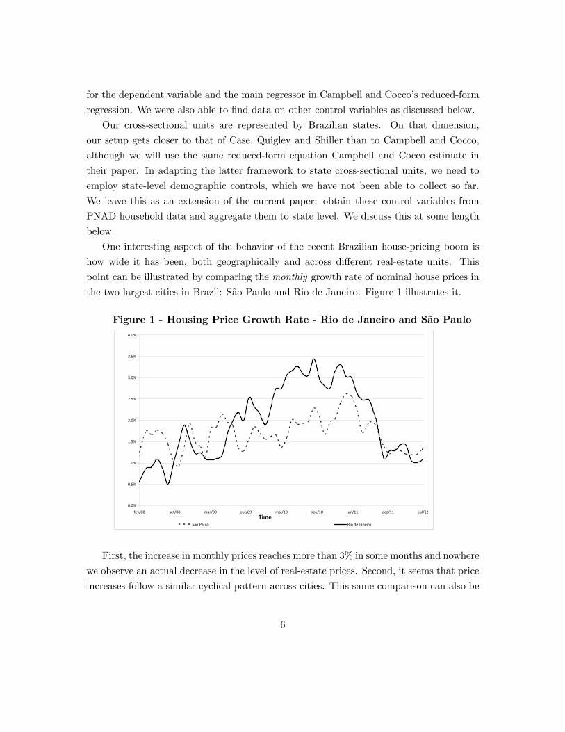
One interesting aspect of the behavior of the recent Brazilian house-pricing boom is

how wide it has been, both geographically and across di¤erent real-estate units. This

point can be illustrated by comparing the monthly growth rate of nominal house prices in

the two largest cities in Brazil: São Paulo and Rio de Janeiro. Figure 1 illustrates it.

Figure 1 - Housing Price Growth Rate - Rio de Janeiro and São Paulo

0.0%

0.5%

1.0%

1.5%

2.0%

2.5%

3.0%

3.5%

4.0%

fev/08 set/08 mar/09 out/09 mai/10 nov/10 jun/11 dez/11 jul/12

São Paulo Rio de Janeiro

Time

First, the increase in monthly prices reaches more than 3% in some months and nowhere

we observe an actual decrease in the level of real-estate prices. Second, it seems that price

increases follow a similar cyclical pattern across cities. This same comparison can also be

6

made when we analyze the nominal growth rate in prices for apartments with di¤erent

sizes (number of bedrooms); see Figure 2.3

Figure 2 - Housing Price Growth Rate by Number of Bedrooms

1%

0%

1%

2%

3%

4%

5%


São Paulo 1 bedroom Rio de Janeiro 1 bedroom

0%

1%

2%

3%

4%

5%


São Paulo 2 bedrooms Rio de Janeiro 2 bedrooms

0%

1%

2%

3%

4%

5%



0%

1%

2%

3%

4%

5%



There are several factors that could explain this sharp increase in real-estate prices in

Brazil in the recent past. The �rst is the decrease in real interest rates. The Brazilian

basic interest rate (Selic) was set as 17:25% a.a. by the Central Bank of Brazil in early

2006 and had decreased to 8% a.a. in the middle of 2012, while in�ation had increased

in this period. Thus, the reduction of the real rate of interest in Brazil was even larger.

As a consequence, we observed a sharp increase in real-estate credit for this period. The

second is an increase in the purchasing power of the Brazilian middle class: minimum wage

has increased above in�ation in the recent past and the Brazilian government adopted a

myriad of social programs, all of which transferred income to poor and middle-income

families. Third, the income of government, private �rms, and individuals, increased due3 In the Appendix, we present the evolution of the house prices for each state considered in this study.

7

the commodity-price boom experienced in the last 10 years.

Our empirical results are as follows. First, we �nd a positive e¤ect of house-price

growth on non-durable consumption growth in Brazil. Second, this e¤ect is smaller that

found in the U.K. by Campbell and Cocco (2007). In Brazil, house-price elasticity estim-

ates are in the range 0:23 to 0:27.

The remainder of the paper is organized as follows. Section 2 describes the model

and the data considered. Section 3 presents the estimation methodology and the results.

Finally, Section 4 concludes the paper.

2 The Model and the Data

2.1 Model

We follow Campbell and Cocco (2007) that introduce their model of housing choice, fur-

ther used to simulate data. They consider that household i derives utility during month

t from housing services, Hit, and non-durable goods, Cit. In particular, the authors as-

sume time additive preferences that are separable between housing and non-durable goods

consumption:

u(Cit;Hit) =C1� it

1� + �H1� it

1� :

Separability in preferences eliminates possible substitution e¤ects when the price of

housing services increase, and is an important feature of their setup. In each period, the

agent decides not only on Hit and Cit, but also if it is optimal to rent or to buy real

estate. Let small-cap letters denote variables in log. Then, (logged) real labor income is

exogenous and stochastic, represented as:

yit = f(t; Zit) + vit + wit;

where f(t; Zit) is a function of time (also interpreted as age here) and of other household

characteristics Zit. The components vit and wit are two stochastic components. One is

transitory and the other persistent. The transitory component is captured by the shock

wit �i.i.d., Normal, with mean zero and variance �2w. The persistent component follows

a random walk: vit = vit�1 + �it, where �it is i.i.d., Normal, with mean zero and variance

�2�.

Formally, to model house prices, they assume �uctuations over time. So, the real house

8

price growth rate is given by:

�pit = g + �it;

where g is a constant and �it is a shock that is normally distributed.

On the �nancial side, Campbell and Cocco assume that �there is a single �nancial

asset with riskfree interest rate Rt, in which households may invest. Homeowners may

also borrow at this rate, up to the current value of the house minus a down payment.�

Thus, households face a borrowing constraint given by:

Dit � (1� d)PitHit

where Dit is household�s outstanding debt, d is the down payment proportion and Pit is

the house price. Thus, at any time, the value of the house, net of down payment, debt

cannot be larger than smaller than household�s outstanding debt.

Campbell and Cocco allow homeowners to borrow against the value of their house at

the riskfree rate. Because of this they also rule out default:

Dit (1 +R) � (1� �)Pit+1Hit + Yit+1;

where Pit+1 and Yit+1 are the lower bounds in house prices and labor income in period

t+ 1, respectively, and � represents transaction costs in selling the real-estate property.

Their �nal baseline reduced-form regression takes the form:

�ci;t = �0 + �1rt + �2�yi;t + �3�pi;t + �4�mi;t + �5�Zi;t + �i;t; (1)

i.e., they regress the growth rates of non-durable consumption goods (�ci;t) on the growth

rates on house prices (�pi;t), controlling for real growth rate in income (�yi;t), real growth

rate in household�s mortgage (�mi;t), changes of demographic variables � augmented

with seasonal dummies for the growth rates of non-durable consumption (�Zi;t). One

additional regressor is rt, the (log) real interest rate between periods t and t � 1. It

shows up due to standard intertemporal substitution arguments. Expected signs of the

��s are the following: �rst, a negative standard intertemporal substitution e¤ect for non-

durables, which means �1 > 0; then, in the sense that a positive income surprises should

a¤ect consumption positively it is identi�ed �2 > 0. Most of all, to �t the �ndings of

a positive correlation between non-durable consumption and house prices found in the

9

literature, �3 > 0. We can test the latter with a standard one-sided t-ratio test.

After a parametrization of the model, it is simulated and they concluded that the

discrepancy between simulated data and its estimation results could be assigned to meas-

urement error. So, to assess the Brazilian case, and taking into account our data lim-

itations, we chose to estimate the baseline equation (1) using panel data on states, not

on cohorts of households. The key hypothesis to be tested in this paper is whether rising

house prices may stimulate consumption of non-durable goods, and what is the magnitude

of this impact.

2.2 Data

Our goal is to investigate the response of household non-durable consumption to a change

in house prices in Brazil. As already mentioned, our best household survey � PNAD,

Pesquisa Nacional por Amostra de Domicílios �is incomplete regarding wealth and con-

sumption data. The other household survey, POF �Pesquisa de Orçamentos Familiares,

has household consumption data but it is collected only at a 7- or 8-year interval, yielding

a synthetic panel using POF useless for our purposes, since consumption data would have

little time variation. Thus, we are forced to work with consumption data for Brazilian

states, available from a third survey, PMC �Pesquisa Mensal do Comércio, collected by

IBGE �Instituto Brasileiro de Geogra�a e Estatística.

A monthly index of disaggregated consumption data were obtained from PMC from

February 2008 through July 2012. From it, we are able to construct the growth rate of

total non-durable consumption with proper participation weights for the states of São

Paulo, Rio de Janeiro, Minas Gerais, Ceará, Pernambuco, Bahia and Distrito Federal.

For every state, we de�ned total non-durable consumption as the sum of the following

consumer-good categories (with respective weights in parenthesis4): fuels and lubricants

(8%), hypermarkets, supermarkets, food products, beverages and tobacco (65%); clothing

and shoes (10%), pharmaceutical articles, medical, orthopedic, perfumery and cosmetics

(12%); books, newspapers, magazines and stationery (2%); and other personal articles and

of domestic use (3%). These participation weights were obtained from the POF survey

of 2008-2009, done at the beginning of our sample. With participation weights and the

growth rates of the disaggregated indices in each category and every state, we are able to

4PMC series which we did not consider fell on the following categories: hypermarkets (other), furnitureand household appliances, o¢ ce equipment and supplies, computer and communication.

10

compute the monthly growth rate of total non-durable consumption in every state, which

is our dependent variable (�ci;t) in equation (1).

The explanatory variables in equation (1) were obtained from various sources. The

risk-free interest rate considered here is Selic, the basic interest rate on loans from the

Central Bank of Brazil to the �nancial sector. The Interbank Certi�cate of Deposit rate

(CDI) was also used as a robustness check, but the results are very similar, therefore

dropped. Selic was used as follows: rt = ln(1 + Rt), where Rt is Selic in real terms �

de�ated by the Broad National Consumer Price Index (IPCA).

State income growth rates (�yi;t) used the regional data from IBC-Br �the Regional

Economic Activity Index, constructed by the Central Bank of Brazil. The only state for

which IBC-Br is not available is Distrito Federal (DF), and we used as a proxy the income

growth rate for the Midwest region as a whole (includes Distrito Federal). An alternative

series for (�yi;t) was constructed following Issler and Notini (2013). We interpolate the

annual state GDP to monthly frequency using the IBC-Br as a covariate. We also test

for another monthly covariables as unemployment rate and industrial production, but the

�rst results were satisfactory. The results with this alternative approach are present in

Appendix.

Regarding house-price data, (�pi;t), the source was FipeZap. In particular, we used

the growth rates of the Índice FipeZap de Preços de Imóveis Anunciados. It does not

contain actual transaction prices (market prices) but ask prices on advertised real-estate

properties. It should be noted that, even though the data used is not the transaction prices,

we believe that there is a strong correlation between the transaction and the advertised

prices. Also, we belive that the error brought by this measure is not correlated with

regression residuals.

Data are available for the cities of São Paulo, Rio de Janeiro (RJ), Belo Horizonte

(stae of MG), Fortaleza (state of CE), Recife (state of PE), Salvador (state of BA) and

Brasilia (Distrito Federal �DF). Here, we were forced to use real-estate price data for

the state capital in each state, since state-wide data were not available. We should note

that São Paulo and Rio de Janeiro have longer span on real-estate price data vis-a-vis

other state capitals (starts in February 2008). Other state capitals have data since 2009

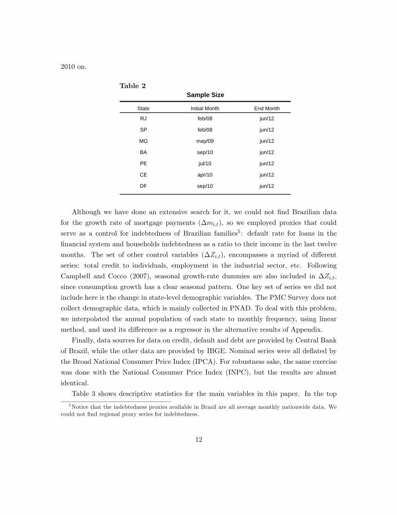
or 2010, making ours an unbalanced panel. Table 2 shows the sample size available for

each of them. There is also a national index real-estate price but it is only available from

11

2010 on.

Table 2

State Initial Month End Month

RJ feb/08 jun/12

SP feb/08 jun/12

MG may/09 jun/12

BA sep/10 jun/12

PE jul/10 jun/12

CE apr/10 jun/12

DF sep/10 jun/12

Sample Size

Although we have done an extensive search for it, we could not �nd Brazilian data

for the growth rate of mortgage payments (�mi;t), so we employed proxies that could

serve as a control for indebtedness of Brazilian families5: default rate for loans in the

�nancial system and households indebtedness as a ratio to their income in the last twelve

months. The set of other control variables (�Zi;t), encompasses a myriad of di¤erent

series: total credit to individuals, employment in the industrial sector, etc. Following

Campbell and Cocco (2007), seasonal growth-rate dummies are also included in �Zi;t,

since consumption growth has a clear seasonal pattern. One key set of series we did not

include here is the change in state-level demographic variables. The PMC Survey does not

collect demographic data, which is mainly collected in PNAD. To deal with this problem,

we interpolated the annual population of each state to monthly frequency, using linear

method, and used its di¤erence as a regressor in the alternative results of Appendix.

Finally, data sources for data on credit, default and debt are provided by Central Bank

of Brazil, while the other data are provided by IBGE. Nominal series were all de�ated by

the Broad National Consumer Price Index (IPCA). For robustness sake, the same exercise

was done with the National Consumer Price Index (INPC), but the results are almost

identical.

Table 3 shows descriptive statistics for the main variables in this paper. In the top

5Notice that the indebtedness proxies avaliable in Brazil are all average monthly nationwide data. Wecould not �nd regional proxy series for indebtedness.

12

panel, it shows that the average consumption growth is high: 1:6% per month. The house

price growth rate remains around 0:9% per month �higher than that of IPCA �which

average monthly growth rate was 0:46%.

Table 3.A

Variable Average Minimum Maximum

∆c 0.016 0.26 0.42

r 0.003 0.007 0.016

∆y 0.001 0.04 0.04

∆p 0.009 0.02 0.03

Descriptive Statistics

The regional growth rates show that Pernambuco, Rio de Janeiro and São Paulo present

the highest average of real house price growth rate. For example, in July 2010, Rio de

Janeiro presented an average increase of 3:3% in the house prices versus a decrease of

13

�0:16% IPCA.

Table 3.B

Variables State∆c∆y∆p∆c∆y∆p∆c∆y∆p∆c∆y∆p∆c∆y∆p∆c∆y∆p∆c∆y∆p

Average for State

RJ0.0153600.0019720.014594

MG0.0154320.0003710.009341

SP0.0158900.0019720.012325

PE0.0184320.0014890.015017

BA0.0209400.0018270.000613

DF0.0137090.0022280.006687

CE0.0162120.0033830.006991

3 Estimation Results and Discussion

3.1 Empirical Results

Equation 1, repeated here for the sake of completeness, was estimated using panel-data

techniques with �xed e¤ects (cross section), with its error term �i;t being decomposed as

follows:

�ci;t = �0 + �1rt + �2�yi;t + �3�pi;t + �4�mi;t + �5�Zi;t + �i;t;

�i;t = ai + ui;t:

14

where ai is a random variable with no time variation and ui;t is a purely idiosyncratic

error, although it may be dependent across time and cross-sectional units. This poses no

problem in estimation, since all it requires for proper inference is some type of White-type

correction in constructing parameter estimates, with their standard errors being robust to

serial correlation and heteroskedasticity of unknown form.

Table 4

Independent Variable (i) (ii) (iii) (iv) (v) (vi) (vii) (viii) (ix) (x)

Real interest rate 0.24 0.41 0.41 0.52 0.11 0.29 0.61 0.40 3.27 13.97(0.309) (0.43) (0.33) (0.44) (0.24) (0.40) (0.52) (0.48) (1.90) (4.26)

∆y 0.27 0.10 0.28 0.16 0.10 0.16 5.28 1.91(0.16) (0.10) (0.18) (0.11) (0.102) (0.109) (5.22) (1.79)

∆p 0.23 0.24 0.27 0.42(0.11) (0.11) (0.11) (0.21)

∆pnac 0.32 0.32 0.28 0.20(0.111) (0.119) 0.13 (0.53)

∆p ∆pnac 0.24 0.31(0.18) (0.18)

∆endiv 0.002 0.06 0.001 0.06 0.001 0.05 0.05 0.04(0.007) (0.02) (0.007) (0.022) (0.007) (0.01) (0.019) (0.018)

∆inad 0.007 0.006 0.007 0.006 0.009 0.003 0.006 0.003(0.006) (0.009) (0.006) (0.009) (0.006) (0.009) (0.009) (0.010)

∆pessoalocup 0.0005 0.0006 0.0006(0.0001) 0.0005 (0.0005)

R² 0.9615 0.9694 0.9610 0.9694 0.9615 0.9702 0.9696 0.9705 0.7862 0.9025N 7 7 7 7 6 6 7 6 7 7T 53 22 53 22 53 22 22 22 51 21

Sample Size 239 154 239 154 217 132 154 132 225 147

Balanced No Yes No Yes No Yes Yes Yes No Yes

Regression Results of the Basic Equation

Table 4 presents estimation results of equation 1 in ten di¤erent speci�cations. The

dependent variable is �ci;t. Variable �pnac is the real growth in house prices of the na-

tional index mentioned above, while �endiv, �inad, and �pessoalocup denote changes

in households indebtedness ratio, default rate for loans, and employment in the indus-

trial sector, respectively. The latter (�pessoalocup) is not available for Distrito Federal

(Brasília) but it is available for all other states.

In some cases we estimate a balanced panel, but we have unbalanced panel estimation

as well. In regressions (i)-(viii) we impose strict exogeneity of the regressors, conditional

on the unobserved e¤ect ai. Thus, estimation of the ��s is performed using the so called

�xed-e¤ects estimator, which is the pooled OLS estimator on time-demeaned data. The

15

latter eliminates ai from the system. Since the error term is dynamically incomplete

and possibly heteroskedastic, robust inference has to be conducted to account for time-

depedence and heteroskedasticity of unknown form. In regressions (ix) and (x) we relax the

strict-exogeneity assumption and apply instrumental-variable techniques, while keeping

robust inference due to the nature of the error term. Details of estimation results are as

follows:

1. In speci�cations (i) and (ii), the estimated coe¢ cients for rt, �yi;t and �pi;t are

positive, but only that of the real growth in house prices is statistically signi�c-

ant. Besides, signi�cance is stronger when the national index was used as the price

regressor.

2. In speci�cations (iii) and (iv), the real growth in income �yi;t was excluded and

conclusions did not change.

3. In speci�cations (v) and (vi), we excluded Distrito Federal (Brasília) from the system,

since �pessoalocup is not available for it. Then, we are able to include this regressor

in the analysis. Once more, changes in house prices are relevant to explain changes

in consumption.

4. In speci�cations (vii) and (viii), we experiment with the di¤erence between the real

growth in local house price and the real growth in national house price �p��pnac.This results in a non-signi�cant relationship between house prices and non-durable

consumption.

5. For regressions (i)-(viii), we found that house-price elasticity point estimates in the

range 0:23 to 0:27. Hence, an increase of 1% in house prices leads to a maximum

increase of 0:27% in non-durable consumption. Such elasticity is much lower than

one found by Campbell and Cocco for the U.K.: range of 0:57 to 1:58. Possibly,

Brazilian households have a much higher borrowing constraint than the one facing

U.K. households. This is possibly due to the fact that the U.K. �nancial sector is

much more developed then its Brazilian counterpart.

6. For regressions (ix) and (x) we use instrumental-variable techniques, where the in-

struments were lags of the explanatory variables. These results show the importance

of using local house prices instead of national. In the �rst case, we found an elasti-

16

city of house prices of 0:42, which is closer to the lower estimates of Campbell and

Cocco, 0:57.

As a �nal exercise, we estimate equation 1 using only data for the two most important

Brazilian states �Rio de Janeiro and São Paulo �which are the two cross-sectional units

with the longest time span: February 2008 through June, 2012. Results are shown in

Table 5. The estimation was done under the instrumental-variable techniques, the same

techinique for regressions (ix) and (x) in Table 4. Although regional house prices are very

signi�cant in (i), the same is not true when we use the national house pricing index in (ii).

Table 5

Independent Variable (i) (ii)

Real interest rate 1.43 3.41(0.17) (5.78)

∆y 1.15 1.95(0.91) (1.26)

∆p 0.16(0.05)

∆pnac 0.19(0.45)

R² 0.9595 0.9665N 2 2T 51 20

Sample Size 102 40

Balanced Yes Yes

Regression Results of the Basic Equation (SP and RJ)

3.2 Discussion

First and foremost, we should emphasize that there is an unequivocal positive and signi-

�cant e¤ect of house prices on non-durable consumption in Brazil. Second, this e¤ect is

smaller that found in the U.K. by Campbell and Cocco (2007). In our view, these two

results allow the evaluation of two competing explanations for the existence of the positive

correlation between house prices and non-durable consumption.

Campbell and Cocco give two potential explanations for the existence of a positive

correlation between house prices and non-durable consumption for households: (a) by a

direct wealth e¤ect due to the increase in real-estate prices, and (b) by relaxing borrowing

17

constraints the household is subject to. On the absence of substitution between non-

durables and durables, one should not expect (a) to be a plausible explanation. Housing

is a commodity, and its higher price is simply a compensation for higher rent. So, using

a present-value argument, the increase in the price of real estate must be exactly o¤set

by the expected present-discounted value of rent. Hence, in expected present-value terms

there is no change in the budget constraint for the household, and there can be no wealth

e¤ect. The second explanation (b) is more plausible since real-world consumers are subject

to borrowing constraints. In this case, an increase in house prices triggers re-�nancing the

house. The additional borrowing can be used to smooth consumption over the life cycle.

This e¤ects should be bigger the more developed the �nancial sector. It should also be

di¤erent across households. Young renters are �short�on housing (want to buy) whereas

old owners are �long,�since they want to change a larger house for a smaller one.

The comparison of the results found here and in Campbell and Cocco for the estimation

of equation 1, give little support for the �rst explanation (a) and a lot of support for the

second explanation (b). First, as we argued in the Introduction, the share of real-estate

in wealth is larger in Brazil than in U.S. (and probably for the U.K. as well). Hence, if

explanation (a) were true, we should have found a larger house-price elasticity for Brazil,

which was not the case. Second, if explanation (b) was true, we should expect a higher

house-price elasticity for the U.K. vis-a-vis that of Brazil, simply because the �nancial

sector in the former is more developed than that of the latter. These are exactly our

�ndings.

4 Conclusions and Further Research

In this paper we examine the impact of changes in house prices on the growth rate of

non-durable consumption expenditures, testing whether this e¤ect is positive once we

use appropriate controls. Our study mixes the framework of Case, Quigley and Shiller

(2005) and Campbell and Cocco (2007). The interesting feature of Campbell and Cocco

is that they tried to understand the economics of how these �uctuations in house prices

a¤ect households�consumption decisions, identifying important channels that could explain

changes in the latter. They build and simulate a structural model for household optimal

decisions and �nd some channels that could lead to a positive e¤ect. On the other hand,

Case, Quigley and Shiller have a data base that is closer to ours: state-level data for

consumers instead of the household data employed by Campbell and Cocco.

18

Our �rst �nding is that there is a positive and signi�cant e¤ect of house prices on

non-durable consumption in Brazil. Second, this e¤ect is smaller that found in the U.K.

by Campbell and Cocco (2007). We found that house-price elasticity point estimates are

in the range 0:23 to 0:27. Hence, an increase of 1% in house prices leads to an increase of

about 0:25% in non-durable consumption in Brazil. This is much lower than what Camp-

bell and Cocco found for the U.K.: ranging from 0:57 to 1:58. In our view, these two pieces

of evidence point toward a �nancial explanation for the positive correlation between house

prices and non-duarable consumption, which rely on the existence of liquidity constraints

faced by households that are relaxed once the price of a house he/she owns increases.

References

[1] Bernanke, B., Gertler, M. and Watson, M. (1997). Systemic monetary policy and the

e¤ects of oil price shocks. Brooking Papers on economic activity, (1): 91-157.

[2] Bertaut, C.C., Starr-McCluer, M. (2002). Household Portfolios in the United States.

In: Guiso, L., Haliassos, M., Jappelli, T. (Eds.), Household Portfolios. MIT Press,

Cambridge, MA Chapter 5.

[3] Bernanke, B. (1985). �Adjustment Costs, Durable Goods and Aggregate Consump-

tion,�Journal of Monetary Economics, vol. 15, pp. 41�68.

[4] Bhalla, S.S. (2009). �The middle class kingdoms of India and China.�Mimeo.

[5] Browning, M. and Crossley, T. (2000), �Luxuries are Easier to Postpone: A Proof �,

Journal of Political Economy, 108 (5), 1064�1068.

[6] Cameron, A. C. and Trivedi, P. (2005). Microeconometrics: methods and applica-

tions". Cambridge University Press.

[7] Campbell, J.Y. e Cocco, J.F. (2007). "How do house prices a¤ect consumption? Evid-

ence from micro data". Journal of Monetary Economics, v. 54: 591-621.

[8] Case, K.E., Quigley, J. and Shiller, R.J. (2005). "Comparing wealth e¤ects: the stock

market versus the housing market",The B.E. Journal of Macroeconomics, v.5 (1).

[9] Gan, J. (2010). "Housing Wealth and Consumption Growth: Evidence from a Large

Panel of Households," Review of Financial Studies, 23 (6): pp. 2229-2267.

19

[10] Hofman, A. (1992). "Capital accumulation in Latin America: a six country compar-

ison for 1950-89". Review of Income and Wealth, v38 (4): 365-391.

[11] _______. (2000)."Standardised capital stock estimates in Latin America: a 1950-

94 update". Cambridge Journal of Economics, v 24 (1): 45-86.

[12] Hryshkoa, D., Luengo-Prado, M. J. and Sørensen, B.. (2010). "House prices and risk

sharing," Journal of Monetary Economics, Vol. 57, Issue 8, pp. 975�987.

[13] Issler, J.V. and Notini, H. (2013), �Estimating Brazilian Monthly Real GDP: a State-

Space Approach�, Mimeo. EPGE, FGV.

[14] Issler, P.F. (2013), "Durability and the Consumption Cycle," Ph.D. Thesis, Haas

School of Business, University of California at Berkeley.

[15] Laibson, D. and Mollerstrom, J. (2010). "Capital Flows, Consumption Booms and

Asset Bubbles: A Behavioural Alternative to the Savings Glut Hypothesis," Economic

Journal, Volume 120, Issue 544, pp. 354�374.

[16] Lustig, H. and Van Nieuwerburgh, S. (2006). How much does household collateral

constrain regional risk sharing? UCLA and NYU, unpublished paper.

[17] Marquetti, A. (2000). �Estimativa do Estoque de Riqueza Tangível no Brasil�. Nova

Economia, v. 10 (2): 11-37.

[18] Mönch, E. and Uhlig, H. (2005). "Towards a Monthly Business Cycle Chronology for

the Euro Area". Journal of Business Cycle Measurement and Analysis 2(1).

[19] Morandi, L. (1998). �Estoque de Riqueza e a Poupança do Setor Privado no Brasil -

1970/95�. IPEA: Texto para discussão. n 572.

[20] Neri, M.C. et al. (2008), "Poverty and the new middle class in the decade of equal-

ity." www.fgv.br/cps/desigualdade version 1 and 2, Rio de Janeiro, Fundação Getulio

Vargas.

[21] Ogaki, M. and Reinhart, C. (1998). �Measuring Intertemporal Substitution: The Role

of Durable Goods,�Journal of Political Economy, 106(5), 1078-98.

[22] Piazzesi, M., Schneider, M. and Tuzel, S. (2007). "Housing, consumption and asset

pricing", Journal of Financial Economics, Volume 83, Issue 3, pp. 531-569.

20

[23] Ravallion, M. (2009) �The developing world�s bulging (but vulnerable) �middle class��,

World Bank Policy Research Working Paper No. 4816.

[24] Ren, Y. and Yuan, Y. (2012) "Why the Housing Sector Leads the Whole Economy:

The Importance of Collateral Constraints and News Shocks," The Journal of Real

Estate Finance and Economics, September 2012.

[25] http://www.sidra.ibge.gov.br/

[26] U.S. Census Bureau. (2012) "Statistical Abstract of the United States: 2012. Income,

Expenditures, Poverty, and Wealth," Section 13, pp. 431-470.

[27] Wilson, D. and Dragusanu, R. (2008). �The expanding middle: The exploding world

middle class and falling global inequality�, Global Economic Paper No.170, Goldman

Sachs.

[28] Wogart, J. P. (2010). "Global booms and busts: how is Brazil�s middle class faring?."

Revista de Economia Política [online]. vol.30, n.3, pp. 381-400. ISSN 0101-3157.

[29] Yogo, M. (2006). "A Consumption-Based Explanation of Expected Stock Returns,"

The Journal of Finance, Vol. 61, No. 2 (Apr., 2006), pp. 539-580.

[30] http://www.zap.com.br/imoveis/�pe-zap/

21

Appendix 1Evolution of house-price growth rates for each state considered in this study:

Brasil

0.00%

0.50%

1.00%

1.50%

2.00%

2.50%

3.00%

set/10 jan/11 abr/11 jul/11 nov/11 fev/12 mai/12

Brasil

Bahia (Salvador)

1.5%

1.0%

0.5%

0.0%

0.5%

1.0%

1.5%

2.0%

2.5%

ago/10 nov/10 fev/11 jun/11 set/11 dez/11 abr/12 jul/12

Salvador

Ceará (Fortaleza)

1.5%

1.0%

0.5%

0.0%

0.5%

1.0%

1.5%

2.0%

2.5%

3.0%

3.5%

4.0%


Distrito Federal

0.5%

0.0%

0.5%

1.0%

1.5%

2.0%

2.5%

3.0%

3.5%

4.0%


22

Pernambuco (Recife)

0.0%

0.5%

1.0%

1.5%

2.0%

2.5%

3.0%

3.5%

4.0%


Minas Gerais (Belo Horizonte)

1.5%

1.0%

0.5%

0.0%

0.5%

1.0%

1.5%

2.0%

2.5%

3.0%

3.5%


São Paulo

0.0%

0.5%

1.0%

1.5%

2.0%

2.5%

3.0%


Rio de Janeiro

0.0%

0.5%

1.0%

1.5%

2.0%

2.5%

3.0%

3.5%

4.0%


23

Appendix 2Regression results of the basic equation using interpolated income and interpolated

population.

Independent Variable (i) (ii) (iii) (iv) (v) (vi) (vii) (viii) (ix) (x)

Real interest rate 0.27 0.23 0.41 0.08 0.16 0.19 0.54 0.36 0.19 0.36(0.28) (0.42) (0.34) (0.45) (0.24) (0.42) (0.53) (0.52) (0.35) (0.50)

∆y 0.34 0.16 0.35 0.25 0.16 0.24 0.25 0.11(0.16) (0.13) (0.18) (0.14) (0.12) (0.14) (0.16) (0.16)

∆p 0.20 0.24 0.24 0.16(0.12) (0.12) (0.13) (0.17)

∆pnac 0.78 0.79 0.61 0.22(0.22) (0.23) (0.15) (0.12)

∆p ∆pnac 0.24 0.31(0.19) (0.19)

∆endiv 0.003 0.06 0.001 0.06 0.0005 0.05 0.05 0.04(0.007) (0.02) (0.007) (0.02) (0.006) (0.02) (0.01) (0.02)

∆inad 0.008 0.008 0.007 0.008 0.01 0.004 0.006 0.003(0.006) (0.01) (0.006) (0.009) (0.006) (0.009) (0.009) (0.01)

∆pessoalocup 0.0005 0.0006 0.0006(0.0002) (0.0005) (0.0005)

∆population 7.93E08 8.04E06 3.49E08 7.8E06 1.66E07 5,36E06 7.97E07 4.17E07 9.11E07 9.36E06(4.15E07) (3.71E06) (3.78E07) (3.77E06) (3.44E07) (1.15E06) (1.57E06) (1.68E06) (2.67E07) (4.47E06)

R² 0.9616 0.9696 0.9610 0.9695 0.9616 0.9703 0.9696 0.9705 0.9624 0.9693N 7 7 7 7 6 6 7 6 7 7T 53 22 53 22 53 22 22 22 51 21

Sample Size 239 154 239 154 217 132 154 132 225 147

Balanced No Yes No Yes No Yes Yes Yes No Yes

Regression Results of the Basic Equation

The results obtained from interpolated data (regional income and population) can be

compared to those found in section 3.1 in such aspects:

1. The coe¢ cient of rt is negative in the speci�cations with national index and without

instrumental variables.

2. Signi�cance is stronger when national index was used as the price regressor, as was

found in section 3.1.

3. Estimade coe¢ cients of �population are too small in all of speci�cations.

4. The house-price elasticity point estimates in the range 0.20 to 0.79. The upper

bound is higher than in section 3.1.

24

Independent Variable (i) (ii) (iii)

Real interest rate 1.28 0.52 1.56(0.61) (0.40) (2.23)

∆y 0.27 0.23 1.53(0.40) (1.31) (0.62)

∆p 0.11(0.05)

∆pnac 0.52 0.33(0.14) (0.52)

∆population 4.56E07 6.49E06 2.93E07(7.88E08) (3.20E06) (6.05E07)

R² 0.9641 0.9734 0.9475N 2 2 2T 51 21 51

Sample Size 102 42 102

Balanced Yes Yes Yes

Regression Results of the Basic Equation (SP and RJ)

The same basic equation was estimated with data from São Paulo and Rio de Janeiro

only. The signi�cance is stronger when the national index was used, as can be found

comparing speci�cations (i) and (ii). To take advantage of the larger sample size for São

Paulo and Rio de janeiro, we constructed a new national index using only data of these

two states (and properly respective weights) and estimate speci�cation (iii), but we didn�t

�nd signi�cant coe¢ cients.

25

non-durable consumption and real-estate prices in brazil

Documents