non-domestic portfolio insurance: counting the cost of ... · pdf filenon-domestic portfolio...

i n a s s o c i a t i o n w i t h

Non-domestic portfolio insurance: Counting the cost of using US VIX futures

within Australian portfolios

Jason Scally, University of South Australia

Apr i l 2015

ABOUT ASX

ASX is one of the world’s leading financial market exchanges, offering a full suite of services, including listings, trading, clearing and settlement, across a comprehensive range of asset classes.

As the first major financial market open every day, ASX is a world leader in raising capital, consistently ranking among the top five exchanges globally.

With a total market capitalisation of around $1.5 trillion, ASX is home to some of the world’s leading resource, finance and technology companies. Our $47 trillion interest rate derivatives market is the largest in Asia and among the biggest in the world.

ASX has over 150 years of exchange experience and a highly skilled team of 530 people. We put our customers at the centre of everything we do – 6.7 million share owners, 180 participants, and almost 2,200 listed companies and issuers. Please see our customer charter.

We are helping them to build wealth for the future, manage investment and operating risk, and raise capital to fund growth.

ABOUT FINANCIAL MARKETS RESEARCH CENTRE

The Financial Markets Research Centre (FMRC) undertakes research programs for the development of market quality in the derivatives and its OTC markets. The research effort of the team is devoted to two main areas; examining the macroeconomic context and relevance of derivative and OTC markets, and benchmarking the performance and efficiency of the Australian derivative and OTC industry against other nations with the potential to highlight opportunities for improvement. All research is made publicly available and disseminated through regular academic media including international scholarly conferences, journal publications and a working paper series, media as well as through presentations to industry forums, and industry groups.

ABOUT THE AUTHOR Jason Scally, PhD Researcher, Financial Markets Research Centre

Jason is currently undertaking a PhD (Quantitative Finance) with the FMRC and University of South Australia. This includes significant ongoing collaboration with ASX. He previously completed an MPhil (Applied Statistics) at the University of Queensland, with work experience outside the finance industry, in addition to lecturing and research appointments. His current projects include volatility modeling, forecasting and algorithmic trading, which encompasses a substantial ongoing interest in the portfolio, risk and trade management spheres.

Executive Summary

1

Holders of domestic equity portfolios can hedge a portfolio’s exposure to volatility through the use of instruments such as options and variance swaps.

There are advantages and shortcomings with each alternate. Options, as exchange traded instruments, offer reduced counterparty risk however option strategies designed to hedge volatility require regular adjustment to reduce delta effects. Variance swaps have the advantage of not requiring delta adjustment to maintain volatility exposure but as an OTC instrument variance swaps come with inherent counterparty risk, limited liquidity and limited availability for smaller portfolios. In contrast to both options and variance swaps, VIX (volatility futures) are able to represent purer vega exposure, greater accessibility and liquidity, and they are an exchange traded instrument.

While often moving together, Australian and US equity markets can experience significant periods of divergence in terms of returns and volatility. The hedging of domestic equity portfolio volatility with non-domestic instruments ignores such divergences. In terms of the unit cost for such insurance, domestic portfolio holders pay a greater proportion of returns for a smaller reduction in volatility. The magnitude of this lost hedging benefit ranges from 6% to 17%. Over time, the cost in terms of lost alpha can be significant.

In this research note we quantify this cost by testing this scenario for a variety of portfolios and rebalancing frequencies. Our conclusion being: the average loss of hedging performance through the use of non-domestic VIX-type instruments, is in the order of 12% for a range of portfolio types and rebalancing frequencies.

Jason Scally, University of South Australia

1 Vega is the sensitivity of portfolio returns to changes in volatility.

2

In pursuing improved risk-adjusted performance, portfolio managers are increasingly incorporating products directly linked to volatility. Particularly in environments characterised by greater uncertainty, these series can provide targeted volatility protection for a range of diverse investment strategies. The growth in this new asset class stems from a strong negative correlation with underlying returns. However, employing these products and successfully minimising portfolio volatility requires an understanding of the unique characteristics driving this class. While the need to manage the relationship between returns and volatility is common to all portfolios, the particular emphasis here is upon equity-centric alternatives.

A large body of research highlights the Volatility Risk Premium (VRP) dominating volatility linked series. The VRP in VIX2 options is quantified using synthetically constructed variance swaps on VIX futures in Barnea and Hogan (2012)3. Using this construct, the average difference between realised and implied volatilities within VIX options can be extracted. While previous authors have dissected the variance premium in a variety of other markets4, relatively little attention has focused upon the market for volatility. On average, the premium is -3.26%. Analogously, this is the premium equity portfolio holders will pay for one month of downside protection. This result has a wide range and can experience sharp positive spikes, requiring the careful management of infrequent and large tail risk by insurance sellers – complicating the monetisation of premium collection strategies. The VIX is found to contain predictive power, as in Bekaert and Hoerova (2014)5 – although not for future realised volatility. Decomposing the series into a variance premium and conditional variance of equity returns, yields some significance. The former is capable of predicting stock returns; while the latter provides information regarding future economic activity and instability. The majority of work in this area is US centric and while a domestic market supporting the A-VIX6 is developing, relatively little attention has focused upon the Australian perspective.

Volatility behaves very differently across international markets. As stated by Chiang and Wang (2011)7, during periods of stress volatility can spill-over between markets. These synchronous movements can occur in bursts, with their speed and duration being governed by a variety of known and unknown factors – usually originating in the direction of the dominant market. Conversely, during lower volatility regimes (associated with positive market conditions), volatility tends to be dominated by factors that are specific to home markets. These differences in the magnitude and direction of volatility movements greatly complicates the use of non-domestic volatility instrument within equity portfolios. Quantifying the relative degree of underperformance for Australian portfolios is an under-examined issue.

The remainder of this note is organised as follows. First we discuss the origins of the risk premium within volatility linked instruments. Following, the merits of using options, variance swaps and futures are considered. Next we briefly introduce Australian traded VIX futures series, with the subsequent section discussing the use of non-domestic VIX instruments. This section includes a description of our methodology and the data used for evaluations. Finally, our results are presented and discussed with conclusion and appendix following.

Introduction

2 VIX is a registered Trademark of the Chicago Board Options Exchange (CBOE).3 Barnea, A and Hogan, R. 2012, ‘Quantifying the Variance Risk Premium in VIX Options’, Journal of Portfolio Management, 38(3), pp. 143-148.4 For example, see: Amman, M. and Buesser, R. 2013, ‘Variance risk premiums in foreign exchange markets’, Journal of Empirical Finance, 23, 16-32

and Wu, L. 2011, ‘Variance dynamics: Joint evidence from options and high frequency returns’, Journal of Econometrics, 1(160), pp. 280-287. The CBOE has created indices with the aim of capturing the negative variance premium in S&P 500 constituents. These indices capture the premium by selling S&P 500 options. The BXM index tracks a series which sells at-the-money covered calls, while the PUT index tracks a portfolio which sells at-the-money puts against a cash reserve.

5 Bekaert, G. and Hoerova, M, 2014, ‘The VIX, the variance premium and stock market volatility’, Journal of Econometrics, Pre-publication6 A-VIX is the S&P/ASX 200 VIX index. License is provided by the CBOE.7 Chiang, M. Wang, L. 2011, ‘Volatility contagion: A range-based volatility approach’, Journal of Econometrics, 165(2), pp. 175-189

3

The volatility premium is a defining feature of volatility linked instruments. Over extended periods, a strategy selling volatility products will capture a positive risk premium. In particular, the XIV and ZIV (short- and medium-term inverse volatility ETF series) attempt to capture this premium without the need to take a physical short position.

The premium is a product of the negative correlation that exists between equity returns and volatility. In general, periods characterised by positive returns will be associated with lower volatility regimes. This makes instruments linked to volatility natural alternatives for hedging vega exposures. Equity holders seeking to insure against declining values – resulting from higher volatility8 – pay a premium for this

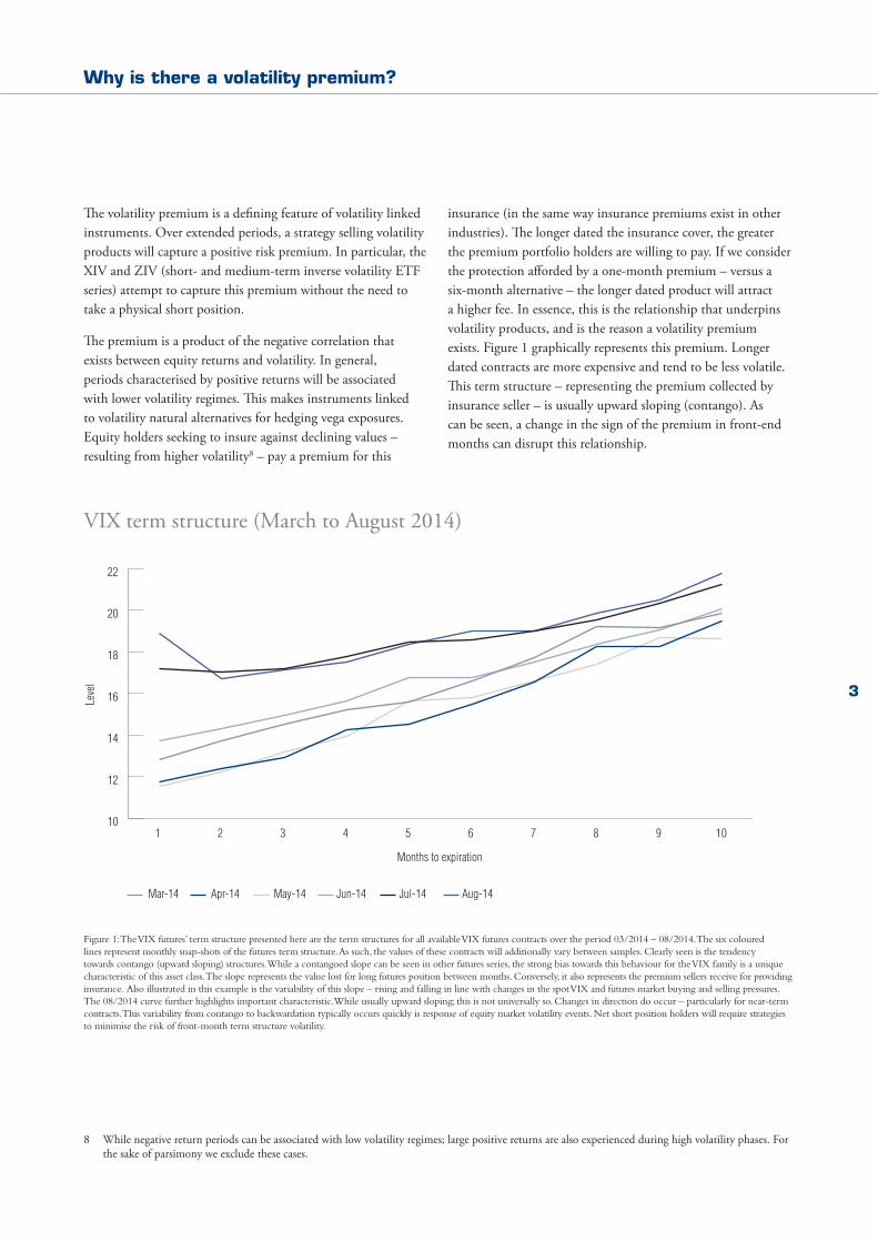
insurance (in the same way insurance premiums exist in other industries). The longer dated the insurance cover, the greater the premium portfolio holders are willing to pay. If we consider the protection afforded by a one-month premium – versus a six-month alternative – the longer dated product will attract a higher fee. In essence, this is the relationship that underpins volatility products, and is the reason a volatility premium exists. Figure 1 graphically represents this premium. Longer dated contracts are more expensive and tend to be less volatile. This term structure – representing the premium collected by insurance seller – is usually upward sloping (contango). As can be seen, a change in the sign of the premium in front-end months can disrupt this relationship.

Figure 1: The VIX futures’ term structure presented here are the term structures for all available VIX futures contracts over the period 03/2014 – 08/2014. The six coloured lines represent monthly snap-shots of the futures term structure. As such, the values of these contracts will additionally vary between samples. Clearly seen is the tendency towards contango (upward sloping) structures. While a contangoed slope can be seen in other futures series, the strong bias towards this behaviour for the VIX family is a unique characteristic of this asset class. The slope represents the value lost for long futures position between months. Conversely, it also represents the premium sellers receive for providing insurance. Also illustrated in this example is the variability of this slope – rising and falling in line with changes in the spot VIX and futures market buying and selling pressures. The 08/2014 curve further highlights important characteristic. While usually upward sloping; this is not universally so. Changes in direction do occur – particularly for near-term contracts. This variability from contango to backwardation typically occurs quickly is response of equity market volatility events. Net short position holders will require strategies to minimise the risk of front-month term structure volatility.

Why is there a volatility premium?

8 While negative return periods can be associated with low volatility regimes; large positive returns are also experienced during high volatility phases. For the sake of parsimony we exclude these cases.

VIX term structure (March to August 2014)

Mar-14 Apr-14 May-14 Jun-14 Jul-14 Aug-14

Leve

l

Months to expiration

1 2 3 4 5 6 7 8 9 1010

12

14

16

18

20

22

4

Volatility sellers collect and volatility buyers pay the VRP. Without a positive premium, sellers would withdraw liquidity due to a lack of financial incentive. Conversely, equity holders would happily purchase low (or no) cost insurance. The resulting buy-side pressure would increase the cost of these insurance like products, to a point where sellers begin to provide liquidity. Thus, the VRP is a dynamic interaction between the point at which expected returns for long equity holders becomes

negative, and expected returns required to incentivise insurance sellers. These varied perspectives, depending upon net long or short exposures, encourage very different participants with specific target outcomes. In general, the average term of long futures holdings is smaller than that of short holdings.

Evidence of the premium can be seen when comparing the VIX9 with 30-day realised volatility. Figure 2 highlights this difference for the 2000 – 2014 period.

Figure 2: The VIX and 30-day realised volatility – here we can clearly see a persistent positive bias between VIX and 30-day realised volatility for the 2000 – 2014 period. Notably, the bias tends to correct from positive, to negative, during periods of market turbulence (characterised by higher volatility phases). A fraction of this difference may be attributable to the estimation of implied volatilities (arising from the use of the classic Black-Scholes-Merton model), and construction methodology underpinning the VIX. However, the bulk of this dispersion arises as a result of the premium equity holders are willing to pay to insure vega exposures. Equity holders need to weight the cost of downside protection (typically in the order of 3-4% monthly) against the expected length the depth of changes in volatility regimes. As with insurance products generally, premiums are lowest when their expected return is low.

As can be seen, the VIX tends to overestimate the level of 30-day realised volatility. It is often asserted that the VIX is a forecast of expected volatility. While not incorrect, it may be more accurate to describe the index as a measure of the premium equity holders are willing to forego for volatility insurance over the next 30-days.

The VIX is constructed using chains of put and call option contracts written on the underlying S&P 500 index. Using the classical Black-Scholas-Merton10 options pricing model,

the current market price of the options are inputted, and the model is solved for volatility. This gives a measure of volatility implied from current prices. In turn, these implied volatilities are aggregated to form the index. In this way, the VIX is a direct result of the buying and selling pressures that exist in underlying options markets. Cetaris paribus, increased pressure from hedgers in underlying options markets will result in increased implied volatility, and in turn; increases in the VIX.

9 Chicago Board Options Exchange, 2003, ‘VIX: CBOE Volatility Index’, Working Paper.10 Black, F. and Scholes, M. 1973, ‘The pricing of options and corporate liabilities’, Journal of Political Economy, 81, pp. 637-659.

The VIX vs 30-day realised volatility

Realised Volatility VIX

Leve

l

2000

2001

2002

2003

2004

2005

2006

2007

2008

2009

2010

2011

2012

2013

2014

0

20

40

60

80

100

5

There exists three common instruments to gain exposure to volatility. While speculation in the movement of volatility is an active area, here we limit our consideration to hedging applications. A particular choice of volatility instrument will depend upon a range of factors, including: ability to and cost of shorting, exactness of volatility exposure required, availability of tradable products matching underlying exposures, investor sophistication and timeframe, counterparty risk tolerance and required price transparency.

Here we consider the use of options, variance swaps and futures. Options are highly dependent upon volatility, because volatility will affect the probability to which an option can expire ’in-the-money’. Increasing implied volatility will make options more expensive by increasing this probability. As previously highlighted, options are important in their own right, and as a pricing mechanism for other volatility linked derivatives.

A position that hedges equity volatility with options can involve puts and/or calls. To complicate the choice, investors will need to consider delta11, as well as vega exposure12. Calls and puts are more responsive to changes in the price of the underlying if their deltas are higher. While a long put provides some downside delta exposure, the degree to which underlying volatility is hedged depends upon the option’s vega. Writing covered puts will provide limited underlying upside equity exposure – through premium compensation. These options can be combined into single and multi-leg strategies aimed at providing particular exposure protection. One alternative (‘short straddle’) combines puts and calls of equal strike price, maturity and size, with the aim of benefiting from decreased implied volatility – while simultaneously mitigating directional price movement exposures13. Delta (and gamma14) neutral positions can be combined into complex cross-market and asset strategies, taking advantage of perceived differences between implied volatilities. The breadth of available strategies is significant, requiring an equivalent ambit of understanding.

These strategies are disadvantaged to a greater extent by changes in the underlying as strike and underlying price diverge. To a degree, this risk can be offset through a physical position in the underlying, in an amount equal to the delta exposure. Delta hedging of this type can be operationally complex – requiring

periodic to frequent rebalancing. While the mechanics of option strategies are beyond the scope of this paper15, we emphasise here the complexity of using options to hedge volatility and interaction between delta and vega.

Variance swaps are a more direct form of volatility exposure. Profit is determined easily. Being the difference between the square of realised volatility and square of implied volatility. A positive expected return is achieved for a short volatility position when realised volatility over the contract’s life is less than the contract implied volatility at initiation. These derivative contracts can be well replicated16, through a static portfolio of options contracts with the same maturity and an equivalent physical underlying position. Generally the burden of rebalancing is only moderate, with a more manageable level of complexity (as opposed to delta-hedging option straddle positions). Unlike options, the vega notional exposure for a variance swap is not dynamic throughout the life of the contract – due to changes in the value of the underlying. However, the notional vega value can still change with significant movements in implied volatility. The result is an increase in the skewness of returns; to a greater extent than experienced by VIX futures contracts. A given increase in implied volatility will result in a larger return impact compared to a similar decrease in implied volatility. This asymmetry is known as ‘convexity’ for long positions, and ’negative convexity’ for short positions. In turn, this feature is beneficial for long positions; and will hurt short positions. Variance swaps are unwound by taking an offsetting position for the remaining life of the initial contract. While the greatest percentage of trading occurs in over-the-counter (OTC) markets, the CBOE’s introduction of variance futures are a means of eliminating cross-party risk, while improving price discovery mechanisms.

A feature of variance swaps used by researchers and hedgers alike, is the convergence of these swaps to the VIX index. Variance swaps written on the S&P 500 and maturing in 30 days will tend to closely approximate the implied volatility index. In part, this stems from the use of similar options strings for replication portfolios17 – highlighting the close relationship shared. While the VIX index can be useful as an indicative proxy of investor sentiment, it is not directly tradable. The closest tradable instruments are VIX futures contracts.

11 Delta is sensitivity of portfolio changes to price changes in the underlying. 12 For simplicity, we limit our discussion here to delta and vega exposures, neglecting theta, rho and lambda.13 McFarren, T. 2013, ‘VIX your portfolio: selling volatility to improve performance, BlackRock Investment Insights, 16(2), pp. 1-22.14 Gamma is a measure of the rate of change in delta, with respect to changes in the underlying.15 Readers are referred to: Morand, B. and Naciri, A. 1990, Options and Investment Strategies, The Journal of Futures Markets, 10(5), pp. 505 - for

further information regarding options in the context of diversification and hedging.16 Hull, J. 2009, Options, futures and other derivatives, 7th edn, Pearson/Prentice Hall.17 Carr, P. and Wu, L. 2006, ‘A Tale of Two Indices’, The Journal of Derivatives, 13(3), pp. 13-29.

Buying and selling volatility

6

If held to maturity, futures contracts written on the VIX can provide a clean exposure to movements in the implied volatility of the S&P 500 index. Their profit is determined as the difference between the spot index level at expiration, and the price of the futures contract at trade initiation. In this way, the current price of a VIX futures contract is the market price of forward implied volatility beginning on expiration date and extending 30 days18. While it is true that the futures series relies upon a pricing signal from the spot index, these derivative contracts are also subject to a variety of other factors. Due to the non-tradable nature of the underlying, there is no unique, closed-form, arbitrage free, cost-of-carry relationship underpinning the connection between index and futures19. While the price of futures will converge to that of the spot as maturity approaches, the futures basis shows no evidence of acting as a predictor for expected changes in implied volatility20.

The underlying VIX index is based on the average of bid-ask prices of options used within index calculations; VIX futures are settled on a Special Opening Quotation (SOQ)21. The SOQ is extracted using actual traded prices of SPX options

during market open on settlement day. This is done to reduce biases induced by the spread. As a result, the VIX futures settlement price and VIX opening price are not necessarily equivalent on settlement day. The value of a VIX futures contract is the underlying VIX value, multiplied by a factor of 100 and a contract multiplier of $1,000. For example, with a VIX value of .1645, the futures contract size is $16,450. The dollar value per tick is $10.00 with a minimum tick size of 0.01 index points. Final settlement date is the Wednesday that is thirty days prior to the third Friday, of the calendar month immediately following the month in which the contract expires (‘Final Settlement Date’). VIX futures contracts settlement involves delivery of a cash settlement amount on the business day immediately following Final Settlement Date.

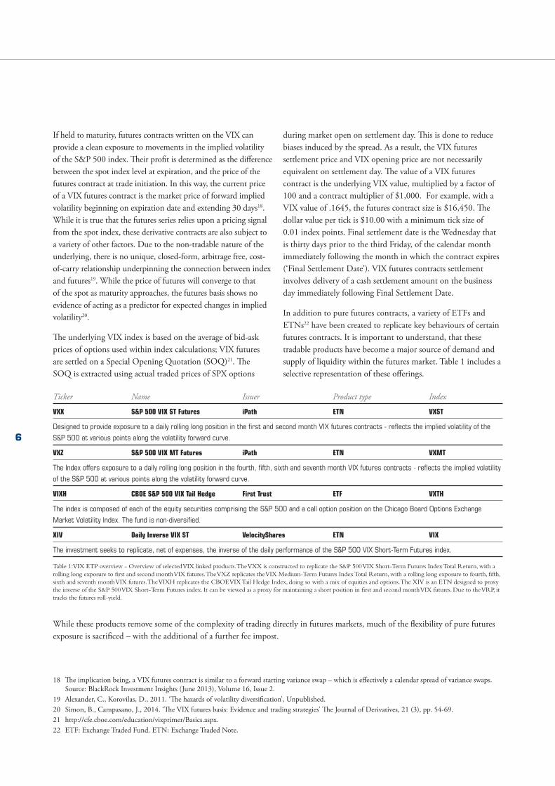
In addition to pure futures contracts, a variety of ETFs and ETNs22 have been created to replicate key behaviours of certain futures contracts. It is important to understand, that these tradable products have become a major source of demand and supply of liquidity within the futures market. Table 1 includes a selective representation of these offerings.

Ticker Name Issuer Product type Index

VXX S&P 500 VIX ST Futures iPath ETN VXST

Designed to provide exposure to a daily rolling long position in the first and second month VIX futures contracts - reflects the implied volatility of the

S&P 500 at various points along the volatility forward curve.

VXZ S&P 500 VIX MT Futures iPath ETN VXMT

The Index offers exposure to a daily rolling long position in the fourth, fifth, sixth and seventh month VIX futures contracts - reflects the implied volatility

of the S&P 500 at various points along the volatility forward curve.

VIXH CBOE S&P 500 VIX Tail Hedge First Trust ETF VXTH

The index is composed of each of the equity securities comprising the S&P 500 and a call option position on the Chicago Board Options Exchange

Market Volatility Index. The fund is non-diversified.

XIV Daily Inverse VIX ST VelocityShares ETN VIX

The investment seeks to replicate, net of expenses, the inverse of the daily performance of the S&P 500 VIX Short-Term Futures index.

Table 1: VIX ETP overview - Overview of selected VIX linked products. The VXX is constructed to replicate the S&P 500 VIX Short-Term Futures Index Total Return, with a rolling long exposure to first and second month VIX futures. The VXZ replicates the VIX Medium-Term Futures Index Total Return, with a rolling long exposure to fourth, fifth, sixth and seventh month VIX futures. The VIXH replicates the CBOE VIX Tail Hedge Index, doing so with a mix of equities and options. The XIV is an ETN designed to proxy the inverse of the S&P 500 VIX Short-Term Futures index. It can be viewed as a proxy for maintaining a short position in first and second month VIX futures. Due to the VRP, it tracks the futures roll-yield.

While these products remove some of the complexity of trading directly in futures markets, much of the flexibility of pure futures exposure is sacrificed – with the additional of a further fee impost.

18 The implication being, a VIX futures contract is similar to a forward starting variance swap – which is effectively a calendar spread of variance swaps. Source: BlackRock Investment Insights (June 2013), Volume 16, Issue 2.

19 Alexander, C., Korovilas, D., 2011. ‘The hazards of volatility diversification’, Unpublished.20 Simon, B., Campasano, J., 2014. ‘The VIX futures basis: Evidence and trading strategies’ The Journal of Derivatives, 21 (3), pp. 54-69.21 http://cfe.cboe.com/education/vixprimer/Basics.aspx.22 ETF: Exchange Traded Fund. ETN: Exchange Traded Note.

7

While domestic VIX futures are a recent introduction to the Australian market, participants familiar with overseas offerings will be able to comfortably incorporate these contracts within equity portfolios. The A-VIX futures contract multiplier is AUD$1,000 times the S&P/ASX 200 VIX futures value, with a minimum tick movement of 0.05 points (equivalent to AUD$50). Contracts expire at 12.00pm on the Tuesday, thirty days prior third Thursday of the following calendar month. The final settlement price is the average value of the S&P/ASX 200 VIX between 11.30am and 12.00pm on the Last Trading Day – with settlement prices calculated to two decimal places. Trading in S&P/ASX 200 VIX Futures began on 21 October 2013. By design, A-VIX futures specification are materially similar to VIX equivalents, making their adoption within domestic equity portfolios intuitive for those already familiar with non-domestic alternatives.

VIX futures in Australia

8

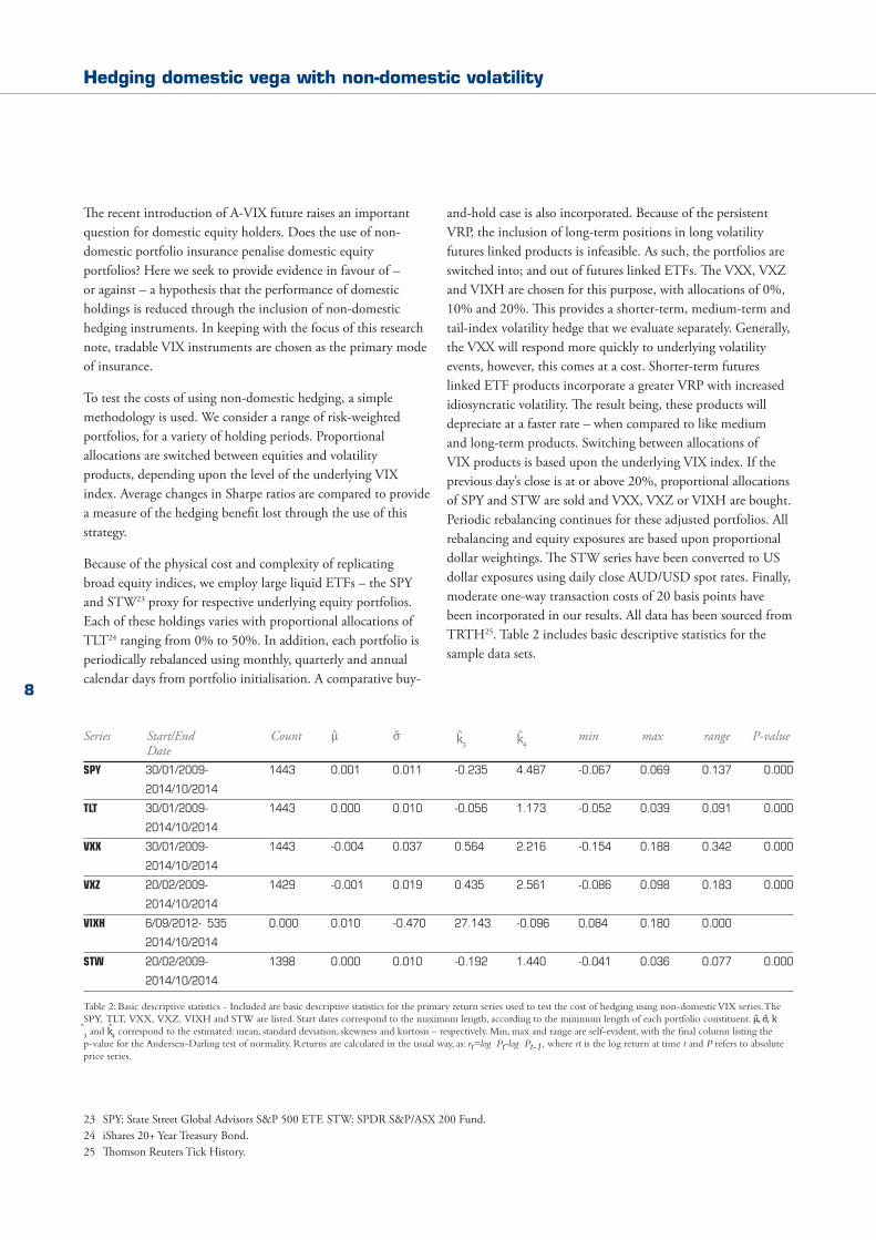
The recent introduction of A-VIX future raises an important question for domestic equity holders. Does the use of non-domestic portfolio insurance penalise domestic equity portfolios? Here we seek to provide evidence in favour of – or against – a hypothesis that the performance of domestic holdings is reduced through the inclusion of non-domestic hedging instruments. In keeping with the focus of this research note, tradable VIX instruments are chosen as the primary mode of insurance.

To test the costs of using non-domestic hedging, a simple methodology is used. We consider a range of risk-weighted portfolios, for a variety of holding periods. Proportional allocations are switched between equities and volatility products, depending upon the level of the underlying VIX index. Average changes in Sharpe ratios are compared to provide a measure of the hedging benefit lost through the use of this strategy.

Because of the physical cost and complexity of replicating broad equity indices, we employ large liquid ETFs – the SPY and STW23 proxy for respective underlying equity portfolios. Each of these holdings varies with proportional allocations of TLT24 ranging from 0% to 50%. In addition, each portfolio is periodically rebalanced using monthly, quarterly and annual calendar days from portfolio initialisation. A comparative buy-

and-hold case is also incorporated. Because of the persistent VRP, the inclusion of long-term positions in long volatility futures linked products is infeasible. As such, the portfolios are switched into; and out of futures linked ETFs. The VXX, VXZ and VIXH are chosen for this purpose, with allocations of 0%, 10% and 20%. This provides a shorter-term, medium-term and tail-index volatility hedge that we evaluate separately. Generally, the VXX will respond more quickly to underlying volatility events, however, this comes at a cost. Shorter-term futures linked ETF products incorporate a greater VRP with increased idiosyncratic volatility. The result being, these products will depreciate at a faster rate – when compared to like medium and long-term products. Switching between allocations of VIX products is based upon the underlying VIX index. If the previous day’s close is at or above 20%, proportional allocations of SPY and STW are sold and VXX, VXZ or VIXH are bought. Periodic rebalancing continues for these adjusted portfolios. All rebalancing and equity exposures are based upon proportional dollar weightings. The STW series have been converted to US dollar exposures using daily close AUD/USD spot rates. Finally, moderate one-way transaction costs of 20 basis points have been incorporated in our results. All data has been sourced from TRTH25. Table 2 includes basic descriptive statistics for the sample data sets.

Series Start/End Count μ σ k

3 k

4 min max range P-value

DateSPY 30/01/2009- 1443 0.001 0.011 -0.235 4.487 -0.067 0.069 0.137 0.000

2014/10/2014

TLT 30/01/2009- 1443 0.000 0.010 -0.056 1.173 -0.052 0.039 0.091 0.000

2014/10/2014

VXX 30/01/2009- 1443 -0.004 0.037 0.564 2.216 -0.154 0.188 0.342 0.000

2014/10/2014

VXZ 20/02/2009- 1429 -0.001 0.019 0.435 2.561 -0.086 0.098 0.183 0.000

2014/10/2014

VIXH 6/09/2012- 535 0.000 0.010 -0.470 27.143 -0.096 0.084 0.180 0.000

2014/10/2014

STW 20/02/2009- 1398 0.000 0.010 -0.192 1.440 -0.041 0.036 0.077 0.000

2014/10/2014

Table 2: Basic descriptive statistics - Included are basic descriptive statistics for the primary return series used to test the cost of hedging using non-domestic VIX series. The SPY, TLT, VXX, VXZ, VIXH and STW are listed. Start dates correspond to the maximum length, according to the minimum length of each portfolio constituent. μ , σ , k 3 and k 4 correspond to the estimated: mean, standard deviation, skewness and kurtosis – respectively. Min, max and range are self-evident, with the final column listing the p-value for the Andersen-Darling test of normality. Returns are calculated in the usual way, as: rt=logPt-logPt-1, where rt is the log return at time t and P refers to absolute price series.

Hedging domestic vega with non-domestic volatility

23 SPY: State Street Global Advisors S&P 500 ETF. STW: SPDR S&P/ASX 200 Fund.24 iShares 20+ Year Treasury Bond.25 Thomson Reuters Tick History.

9

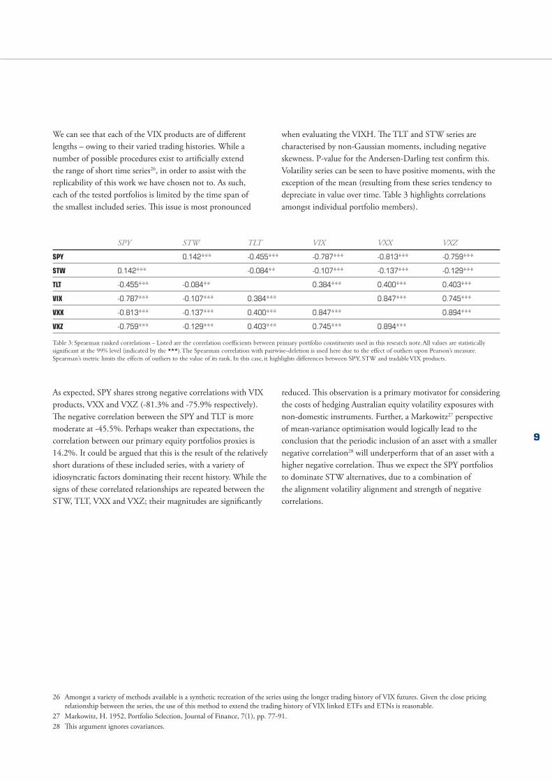
We can see that each of the VIX products are of different lengths – owing to their varied trading histories. While a number of possible procedures exist to artificially extend the range of short time series26, in order to assist with the replicability of this work we have chosen not to. As such, each of the tested portfolios is limited by the time span of the smallest included series. This issue is most pronounced

when evaluating the VIXH. The TLT and STW series are characterised by non-Gaussian moments, including negative skewness. P-value for the Andersen-Darling test confirm this. Volatility series can be seen to have positive moments, with the exception of the mean (resulting from these series tendency to depreciate in value over time. Table 3 highlights correlations amongst individual portfolio members).

SPY STW TLT VIX VXX VXZ

SPY 0.142*** -0.455*** -0.787*** -0.813*** -0.759***

STW 0.142*** -0.084** -0.107*** -0.137*** -0.129***

TLT -0.455*** -0.084** 0.384*** 0.400*** 0.403***

VIX -0.787*** -0.107*** 0.384*** 0.847*** 0.745***

VXX -0.813*** -0.137*** 0.400*** 0.847*** 0.894***

VXZ -0.759*** -0.129*** 0.403*** 0.745*** 0.894***

Table 3: Spearman ranked correlations - Listed are the correlation coefficients between primary portfolio constituents used in this research note. All values are statistically significant at the 99% level (indicated by the ***). The Spearman correlation with pairwise-deletion is used here due to the effect of outliers upon Pearson’s measure. Spearman’s metric limits the effects of outliers to the value of its rank. In this case, it highlights differences between SPY, STW and tradable VIX products.

As expected, SPY shares strong negative correlations with VIX products, VXX and VXZ (-81.3% and -75.9% respectively). The negative correlation between the SPY and TLT is more moderate at -45.5%. Perhaps weaker than expectations, the correlation between our primary equity portfolios proxies is 14.2%. It could be argued that this is the result of the relatively short durations of these included series, with a variety of idiosyncratic factors dominating their recent history. While the signs of these correlated relationships are repeated between the STW, TLT, VXX and VXZ; their magnitudes are significantly

reduced. This observation is a primary motivator for considering the costs of hedging Australian equity volatility exposures with non-domestic instruments. Further, a Markowitz27 perspective of mean-variance optimisation would logically lead to the conclusion that the periodic inclusion of an asset with a smaller negative correlation28 will underperform that of an asset with a higher negative correlation. Thus we expect the SPY portfolios to dominate STW alternatives, due to a combination of the alignment volatility alignment and strength of negative correlations.

26 Amongst a variety of methods available is a synthetic recreation of the series using the longer trading history of VIX futures. Given the close pricing relationship between the series, the use of this method to extend the trading history of VIX linked ETFs and ETNs is reasonable.

27 Markowitz, H. 1952, Portfolio Selection, Journal of Finance, 7(1), pp. 77-91.28 This argument ignores covariances.

10

Having outlined our methodology, here we list and discuss results and limitations. Table 4 highlights our results and primary contribution. For the SPY and STW portfolios, hedged with varying allocations of VXX, the lost adjusted hedging benefit for the STW ranges from 5.7% for the annually rebalanced 50% TLT allocation to 16.5% for the monthly rebalanced 10% TLT allocation. In each of the TLT allocation portfolios, monthly and quarterly rebalance portfolios generally saw the greater reductions in adjusted hedging benefits. While unreported here, the cumulative effects upon returns of more frequent rebalancing tended to outweigh the benefits of maintaining fixed proportional allocations. However, because both equity portfolios are subject to approximately the same transaction cost structure, this affect is not present in our results. Rather, the greater lost benefit for the STW portfolio at higher frequency rebalancing periods is symptomatic of the speed with which the SPY portfolio is able to respond to idiosyncratic volatility events. Viewing rolling estimates of realised volatility for each of these equity offerings confirms this assertion. While some higher volatility regimes spill-over between national exchanges, others remain confined to home markets. The use of a non-domestic volatility hedging instrument ignores this fact. This is, in part, reason for the greater loss in hedging performance during monthly and quarterly rebalancing phases.

Results for the VXZ follow a similar pattern. The greatest loss in adjusted hedging benefit is recorded by the 10% TLT allocation with monthly rebalancing. This loss is 17.1%. The smallest was seen by the 50% TLT allocation with annual rebalancing (6.3%). Again, greater losses in adjusted hedging benefit were experienced by portfolios with more frequent rebalancing. For both the VXX and VXZ cases, the degree of this loss dissipates as we consider portfolios with greater TLT allocations.

For the VIXH case, our results are less clear. Complicating an analysis of the use of this particular product is the lack of significant volatility events which trigger the characteristics of this product. In order to attempt a meaningful analysis we reduced the VIX signal threshold for portfolios switching to allocations of VIXH to 16%. Despite this, total samples within this group remain small. For a moderate 10% TLT allocation, the unit cost of additional risk was negative in the STW case, and only slightly positive for the SPY. The loss of hedging benefit remains generally stable for all other TLT allocations, with a moderate increase as proportions approach 50%. This is reflective of the minimal impact the VIXH has had on these portfolios, and the reduced diversification benefit experienced as a result of the use of a non-domestic treasury linked instrument.

Figure 3 illustrates the cumulative effects of reduced adjusted hedging benefits on the STW portfolio.

Performance loss through non-synchronous volatility use

Figure 3: Unhedged, hedged and simulated hedge STW portfolios – Highlighted here are unhedged, hedged and simulated hedged STW portfolios for 10% TLT allocations with annual rebalancing and VXX hedging. The choice of switching between 0% and 10% VXX is based upon a VIX threshold of 20%. This threshold choice is subjective. The STW series have been converted to a USD denomination using daily AUD/USD spot closing prices. Moderate one-way 20 basis point transaction costs are incorporated. The dark grey series represents the unhedged portfolio; with blue being the hedged alternative. The light grey line illustrates a simulated hedged portfolio. We construct this series by adjusted daily returns to account for reductions in adjusted hedging effectiveness experienced through the use of non-domestic VIX instruments. In this case, because returns (rather than standard deviations) have been adjusted daily, this simulate portfolio represent a best case scenario – should the cost of using non-domestic VIX type hedging instrument be reduced to zero. The y-axis represents cumulative simple returns from a starting value of 0%.

STW, TLT, VXX Portfolio (Unhedged, hedged and simulated hedge)

Unhedged Hedged Simulated hedged

Leve

l

-0.2

-0.0

0.2

0.4

0.6

0.8

1.0

1.2

Feb-

09

Aug-

09

Feb-

10

Aug-

10

Feb-

11

Aug-

11

Feb-

12

Aug-

12

Feb-

13

Aug-

13

Feb-

13

Aug-

14

11

The previous figure includes three portfolios – two real and one simulated. Each incorporates a 10% TLT allocation with 10% of the STW equity position moved to VXX if the VIX closes above 20%. Rebalancing is annual, with AUD/USD changes and transaction costs incorporated. The unhedged portfolio (dark grey line) generates annualised returns of 12.74% with a standard deviation of 13.41%. In the hedged case, returns have increased to 14.17% for an increase in standard deviation to 14.14%. The resulting change in the Sharpe ratio is from 0.95 to 1.00 for the unhedged and hedged portfolios (respectively). As a measure of the reduction in adjusted portfolio benefit resulting from the use of non-domestic VIX instruments, we include the simulated portfolio in the same figure (grey line). To arrive at this hypothetical result, we adjust daily STW portfolio returns by amounts required to produce equivalent Share ratios across like STW and SPY cases. Importantly, because returns – and not variances – are adjusted, this simulated portfolio represents a best-case scenario29. In this optimal exercise, returns increase to 17.42% annually with standard deviations of 15.68%. These differences between unhedged, hedged and simulated hedged continue to grow through time. Referring back to Table 3, the underperformance of hedged STW versus SPY portfolios is intuitive. Including periodic allocations of moderate versus highly negatively correlated assets will lead to sub-optimal allocation decisions and performance outcomes.

This research note is limited in several aspects. Firstly, all sample sizes are small – inducing statistical bias. In this respect we are limited by our chosen methodology. Primarily by the choice to use ETP in lieu of futures contracts. However, this choice was made to increase the differentiability and reproducibility of this note30. Secondly, STW portfolios constructed with TLT (20 year US Govt Bonds) are not entirely realistic. No doubt, Australian portfolio holders would choose an equivalent domestic alternative. In keeping with the theme of this note, our purpose was a comparison of equity portfolio performance given non-domestic VIX instrument inclusion. To reduce the confounding effects of including a variety of dissimilar series, we opted to standardise as many of the portfolio choices as possible. However, a percentage of the final performance results may also be attributable to this decision. Thirdly, we employ delta hedging31, where portfolio value is hedged against price change. Considering the broad objective of utilising VIX-style products is a reduction is equity linked volatility, vega32 hedging may be more appropriate. We leave this issue for a future research note. Finally, related to the small size of the sample, no super-volatility events occur in the 2009-2014 period of the magnitude experienced during 2007-2008. While acknowledging this shortcoming, our evidence suggests our result would have been strengthened if this were the case.

29 Best case in the sense that, differences between SPY and STW Sharpe ratios are simulated using incremental changes to the daily returns of the STW portfolio. A like simulation using variance and return adjustments is not considered here.

30 In this regard, all data and results are available from the author upon request.31 Delta hedging using options is discussed in: Crépey, S. 2004, Delta-hedging vega risk?, Quantitative Finance, 4(5), pp. 559-579 32 Hedging volatility risk is treated in: Zhang, j. Brenner, M. and Ey, O. 2006, Hedging volatility risk, Journal of Banking and Finance, 3(30), pp. 811-821

12

This research note considers the use of VIX instrument within equity portfolios, with the purpose of reducing volatility exposure. We began by outlining the variance risk premium that dominates the volatility asset class, and summarised a number of approaches to hedge this risk. While the use of options and variance swaps have their merits, futures offer a purer exposure to vega. As such, futures linked ETPs form the basis of our analysis. The general problem we consider is from an Australian perspective. Given the recent availability of domestic VIX futures, is this choice of vega hedging instrument optimal when compared to a common non-domestic alternative? In

analysing this issue we consider a number of index based equity portfolios over the 2009-2014 region. Our results show that, the use of non-domestic volatility products results in a persistent and substantial reduction in adjusted hedging benefit. The reduced benefit is in the order of 12%. This leads to a significant erosion of potential alpha over time. If we consider the highly idiosyncratic nature of volatility and cross-border correlations, this result is intuitive. Our results suggest that domestic volatility products will provide a better hedge for domestic equity volatility exposure.

TLT Allocation

Hedge Instrument 10% TLT allocation 20% TLT allocation 30% TLT allocation

VXX

BH M Q A BH M Q A BH M Q A

SPY 2.095 2.271 2.337 2.232 2.027 2.199 2.268 2.168 1.959 2.126 2.196 2.103

STW 1.932 1.949 2.050 2.009 1.871 1.908 2.011 1.981 1.812 1.868 1.969 1.949

% diff -0.084 -0.165 -0.140 -0.111 -0.083 -0.153 -0.128 -0.094 -0.081 -0.138 -0.115 -0.079

VXZ

SPY 2.271 2.326 2.358 2.334 2.203 2.246 2.282 2.263 2.135 2.164 2.204 2.191

STW 2.098 1.986 2.046 2.081 2.038 1.939 2.003 2.049 1.979 1.891 1.956 2.011

% diff -0.082 -0.171 -0.152 -0.123 -0.081 -0.159 -0.114 -0.104 -0.079 -0.144 -0.127 -0.090

VIXH

SPY 0.096 0.099 0.100 0.097 3.248 3.158 3.188 3.257 3.081 2.976 3.008 3.103

STW -0.311 -0.302 -0.301 -0.315 2.903 2.852 2.911 2.924 2.732 2.667 2.728 2.765

% diff -3.087 -3.278 -3.322 -3.079 -0.119 -0.107 -0.095 -0.114 -0.128 -0.116 -0.103 -0.122

Hedge Instrument 40% TLT allocation 50% TLT allocation

VXX

BH M Q A BH M Q A AV

SPY 1.892 2.052 2.122 2.037 1.827 1.976 2.046 1.969 2.177

STW 1.757 1.828 1.926 1.911 1.720 1.786 1.878 1.863 1.937

% diff -0.077 -0.123 -0.097 -0.066 -0.062 -0.106 -0.089 -0.057 -0.124

VXZ

SPY 2.065 2.081 2.123 2.116 1.996 1.996 2.039 2.038 2.168

STW 1.921 1.843 1.908 1.968 1.866 1.794 1.856 1.918 1.943

% diff -0.075 -0.129 -0.113 -0.075 -0.070 -0.113 -0.099 -0.063 -0.116

VIXH

SPY 2.903 2.783 2.819 2.936 2.712 2.579 2.618 2.752 2.376

STW 2.548 2.471 2.533 2.591 2.348 2.259 2.324 2.399 2.036

% diff -0.139 -0.126 -0.113 -0.133 -0.155 -0.142 -0.127 -0.147 -0.167

Table 4: Comparative hedging performance – Included here are summary results for the differences in hedging performance of SPY and STW portfolios. The far left columns include three volatility instrument choices: VXX, VXZ and VIXH. Each horizontal panel corresponds to the average difference returns between the 0%, 10% and 20% VIX instrument additions. These are scaled by the same average measure of standard deviation changes. Columns are classed as buy-and-hold (BH), monthly (M), quarterly (Q) and annually (A) rebalanced. BH portfolios maintain fixed equity/TLT proportions (with a switch to VIX instruments) without any rebalancing. Each figure is a measure of the excess returns gained through proportional allocations of VIX instruments, in terms of units of risk. For example: for the first SPY portfolio with a 10% TLT allocation. The switching of proportional allocations of VXX from SPY has resulted in an average increase of 2.095 units of returns – per unit of risk (adjusted hedging benefit). The bold figures underlying each panel are percentage differences in SPY and STW adjusted hedging benefit. The first figure of 0.078 indicates the cost (in terms of lost adjusted hedging benefit) of using non-domestic products to hedge domestic volatility. The final column in the far right of the table lists the averages of each row. The cut-off chosen for the switching proportional allocations of SPY and STW to VXX and VXZ is a VIX of 20%. For the VIXH this is reduced to 16% - owing to the shorter history of this series and corresponding low realised volatility.

Conclusion

13

The VIX is constructed in a three step procedure33 – beginning with average duration. The VIX is a measure of 30-day implied volatility. Because front-end options will only have 30 days until expiry once, a combination is required. With 12 expiry months annually, bracketing a constant 30-day calendar period requires the weighted average of front and adjacent expiry month options. I.e. the average time to expiry of option A with 15-day to expiry and option B with 45-day to expiry, is 30-days.

As with most derivatives, as expiry nears, pricing anomalies strengthen. To avoid this effect, when the front month options have eight days until expiration, they are phased out of spot VIX calculations, and the second and third months are incorporated.

Secondly, we need to consider which strikes to include. Here also, potential bias exists with the inclusion of deep out-of-the-options that may have non-zero bids. Beginning with at-the-money puts and calls, successive strike prices are used until two successive strikes are reached with zero bids. Because of this, the number of options and range of strike prices will continually change.

Finally, with the term and strikes, available prices for a calculation of implied volatility.

Initially the weighted prices for the entire options strip for each month are added. These weights are formulated to create an options portfolio with a constant exposure to volatility. This process, performed independently for each contract month, generates a single, model-free implied volatility for each of the front and second contract months. These numbers are then interpolated to arrive at a single VIX representation. This process is repeated each 15 seconds (randomised) for spot calculations during regular trading hours.

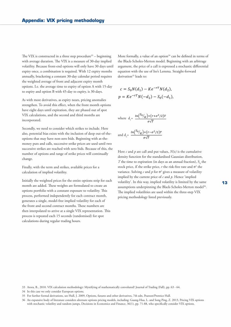
More formally, a value of an option34 can be defined in terms of the Black-Scholes-Merton model. Beginning with an arbitrage argument, the price of a call is expressed a stochastic differential equation with the use of Ito’s Lemma. Straight-forward derivation35 leads to:

where d1=

and d2=

Here c and p are call and put values, N(x) is the cumulative density function for the standardised Gaussian distribution, T the time to expiration (in days as an annual fraction), S0 the stock price, K the strike price, r the risk-free rate and σ2 the variance. Solving c and p for σ2 gives a measure of volatility implied by the current price of c and p. Hence ‘implied volatility’. In this way, implied volatility is limited by the same assumptions underpinning the Black-Scholes-Merton model36. The implied volatilities are used within the three-step VIX pricing methodology listed previously.

Appendix: VIX pricing methodology

33 Arora, B., 2010. VIX calculation methodology: Mystifying of mathematically convoluted? Journal of Trading (Fall), pp. 63 - 64.34 In this case we only consider European options.35 For further formal derivations, see Hull, J. 2009, Options, futures and other derivatives, 7th edn, Pearson/Prentice Hall.36 An expansive body of literature considers alternate options pricing models, including: Guang-Hua, L. and Song Ping, Z. 2013, Pricing VIX options

with stochastic volatility and random jumps, Decisions in Economics and Finance, 36(1), pp. 71-88, who specifically consider VIX options.

17


The VIX is constructed in a three step procedure33 – beginning with average duration. The VIX is a measure of

30-‐day implied volatility. Because front-‐end options will only have 30 days until expiry once, a combination is

required. With 12 expiry months annually, bracketing a constant 30-‐day calendar period requires the

weighted average of front and adjacent expiry month options. I.e. the average time to expiry of option A

with 15-‐day to expiry and option B with 45-‐day to expiry, is 30-‐days.

As with most derivatives, as expiry nears, pricing anomalies strengthen. To avoid this effect, when the front

month options have eight days until expiration, they are phased out of spot VIX calculations, and the second

and third months are incorporated.

Secondly, we need to consider which strikes to include. Here also, potential bias exists with the inclusion of

deep out-‐of-‐the-‐options that may have non-‐zero bids. Beginning with at-‐the-‐money puts and calls,

successive strike prices are used until two successive strikes are reached with zero bids. Because of this, the

number of options and range of strike prices will continually change.


Initially the weighted prices for the entire options’ strip for each month are added. These weights are

formulated to create an options portfolio with a constant exposure to volatility. This process, performed

independently for each contract month, generates a single, model-‐free implied volatility for each of the front

and second contract months. These numbers are then interpolated to arrive at a single VIX representation.

This process is repeated each 15 seconds (randomised) for spot calculations during regular trading hours.

More formally, a value of an option34 can be defined in terms of the Black-‐Scholes-‐Merton model. Beginning

with an arbitrage argument, the price of a call is expressed a stochastic differential equation with the use of

Ito’s Lemma. Straight-‐forward derivation35 leads to:

𝑐𝑐 = 𝑆𝑆!𝑁𝑁 𝑑𝑑! − 𝐾𝐾𝑒𝑒!!"𝑁𝑁 𝑑𝑑! ,

𝑝𝑝 = 𝐾𝐾𝑒𝑒!!"𝑁𝑁 −𝑑𝑑! − 𝑆𝑆! −𝑑𝑑! ,

where 𝑑𝑑! =!" !!

! ! !!!!/! !

! ! and 𝑑𝑑! =

!" !!! ! !!!!/! !

! !. Here 𝑐𝑐 and 𝑝𝑝 are call and put values, 𝑁𝑁 𝑥𝑥 is the

cumulative density function for the standardised Gaussian distribution, 𝑇𝑇 the time to expiration (in days as

an annual fraction), 𝑆𝑆! the stock price, 𝐾𝐾 the strike price, 𝑟𝑟 the risk-‐free rate and 𝜎𝜎! the variance. Solving 𝑐𝑐

and 𝑝𝑝 for 𝜎𝜎! gives a measure of volatility implied by the current price of 𝑐𝑐 and 𝑝𝑝. Hence “implied volatility”.

33 Arora, B., 2010. VIX calculation methodology: Mystifying of mathematically convoluted? Journal of Trading (Fall), pp. 63 -‐ 64. 34 In this case we only consider European options. 35 For further formal derivations, see Hull, J. 2009, Options, futures and other derivatives, 7th edn, Pearson/Prentice Hall.

17


























! ! !!!!/! !

! ! and 𝑑𝑑! =

!" !!! ! !!!!/! !






17


























! ! !!!!/! !

! ! and 𝑑𝑑! =

!" !!! ! !!!!/! !






CONTACT DETAILS

AUSTRALIA Brian GoodmanProduct Development Manager+61 2 9227 0106 [email protected]

ASIAAndrew MusgraveRegional Manager, Asia+61 2 9227 0211 [email protected]

EUROPEJames KeeleyRegional Manager, Europe+44 203 009 3375 [email protected]

Head office ASX Limited Exchange Centre 20 Bridge Street Sydney NSW 2000 Australia

Telephone +61 2 9227 0000

www.asx.com.au

The views, opinions or recommendations of the author in this article are solely those of the author and do not in any way reflect the views, opinions, recommendations, of ASX Limited ABN 98 008 624 691 and its related bodies corporate (“ASX”). ASX makes no representation or warranty with respect to the accuracy, completeness or currency of the content. The content is for information only and does not constitute financial advice. Independent advice should be obtained from an Australian financial services licensee before making investment decisions. To the extent permitted by law, ASX excludes all liability for any loss or damage arising in any way including by way of negligence.

© Copyright 2015 ASX Limited ABN 98 008 624 691. All rights reserved 2015.

non-domestic portfolio insurance: counting the cost of ... · pdf filenon-domestic portfolio...

Documents