noise-sensitive measure for stochastic resonance...

MATHEMATICAL BIOSCIENCES http://www.mbejournal.org/AND ENGINEERINGVolume 3, Number 4, October 2006 pp. 583–602

NOISE-SENSITIVE MEASURE FOR STOCHASTIC RESONANCEIN BIOLOGICAL OSCILLATORS

Ying-Cheng Lai

Department of Electrical Engineering, Arizona State UniversityTempe, AZ 85287

Kwangho Park

Department of Electrical Engineering, Arizona State UniversityTempe, AZ 85287

(Communicated by Yang Kuang)

Abstract. There has been ample experimental evidence that a variety ofbiological systems use the mechanism of stochastic resonance for tasks suchas prey capture and sensory information processing. Traditional quantities forthe characterization of stochastic resonance, such as the signal-to-noise ratio,possess a low noise sensitivity in the sense that they vary slowly about theoptimal noise level. To tune to this level for improved system performance ina noisy environment, a high sensitivity to noise is required. Here we show that,when the resonance is understood as a manifestation of phase synchronization,the average synchronization time between the input and the output signal hasan extremely high sensitivity in that it exhibits a cusp-like behavior aboutthe optimal noise level. We use a class of biological oscillators to demonstratethis phenomenon, and provide a theoretical analysis to establish its generality.Whether a biological system actually takes advantage of phase synchronizationand the cusp-like behavior to tune to optimal noise level presents an interestingissue of further theoretical and experimental research.

1. Introduction. One of the remarkable nonlinear phenomena in biological sys-tems is stochastic resonance (SR), which can roughly be characterized as the opti-mization of certain system performance by noise. Early theoretical evidence sug-gests that noise is essential for the transmission of sensory information, possiblythrough the mechanism of SR [1, 2]. There is also speculation that internal noise ofa biological oscillator may play a constructive role in information transfer throughSR [3]. So far, there have been experimental demonstrations of SR in a varietyof biological systems [4, 5, 6, 7, 8, 9, 10], including the interesting discovery thatSR enhances the electrosensory information available to paddlefish for prey capture[10]. There has even been a psychophysical experiment demonstrating that SRcan be used as a measuring tool to characterize the ability of the human brain tointerpret visual patterns immersed in noise [11].

SR was introduced in 1981 [12, 13] as a plausible mechanism to account for theperiodic occurrence of global glaciation (ice ages). It has stimulated a large amountof research, has been identified in a variety of natural and engineering systems, and

2000 Mathematics Subject Classification. 37H10, 92B99.Key words and phrases. stochastic resonance, phase synchronization, biological oscillators,

FitzHugh-Nagumo (FHN) model.

583

584 YING-CHENG LAI, AND KWANGHO PARK

has continued to be an interesting topic in nonlinear science [14, 15]. Given anonlinear system, its response to a weak signal is generally influenced by noise but,when SR occurs, noise can enhance the response. For periodic signals, a signal-to-noise ratio (SNR) can be defined in terms of the dominant spectral peak in thefrequency domain and can thus characterize the resonance in a natural way [16].For an aperiodic signal, there may be no well-defined peaks in the Fourier spectrum.In this case, the correlation between the input and the output signal [17, 18, 19],entropies, and other quantities derived from the information theory [20, 21, 22,23, 24, 25] can be used for characterization, where SR means the optimization ofsuch a measure by noise. There are also nonlinear systems, in particular excitablesystems, for which the performance optimization can occur in a range of the noiselevel. This is referred to as aperiodic stochastic resonance (ASR) [17, 18, 19].

A general feature associated with existing measures for characterization of SRis that either they vary slowly with noise about the optimal value, exhibiting a“bell-shape” behavior as typically seen in the SNR, or they are insensitive to noisevariation (e.g., the correlation measure in the case of ASR [17, 18, 19]). Because ofthe ubiquity of SR in biological systems [4, 5, 6, 7, 8, 9, 10], a natural question ishow a biological oscillator tunes to the optimal noise level to realize SR. For thispurpose a measure that is highly sensitive to noise variation is desired. There arealso potential technological applications where one might be interested in such anoise-sensitive measure. An example is to develop a device to assess the workingenvironment based on the principle of SR [26, 27, 28, 29]. Specifically, for varioustypes of measuring devices in a noisy environment, it is desirable to have the signalspectral peak as pronounced as possible with respect to the broad, noisy back-ground. The principle of SR can naturally be used to detect the optimal noise level(or the optimal working condition). Ando and Graziani recognized that the SNRis in general not suitable for this purpose, as it does not allow for online tuning ofthe noise variance because of its insensitivity to noise variation about the optimallevel. In a series of papers [26, 27, 28, 29], they developed mathematical modelsutilizing feed-forward estimation theory and tested experimental devices based onthe Schmitt trigger to overcome the difficulty.

In this paper, we present a measure of SR that has an extremely high sensitivityin the sense that, as a function of the noise amplitude, it exhibits a cusp-like behav-ior about the optimal noise level. In particular, recently it has been shown that SRcan be understood as a manifestation of phase synchronization between the inputand the output signal. The relationship between SR and phase synchronizationhas been demonstrated in noisy bistable systems [30, 31, 32, 33, 34, 35, 36, 37]and in excitable systems with periodic [38, 39] and with aperiodic signals [40]. Tosee how SR can be studied through phase synchronization, imagine an input signalxin(t) that oscillates in time. A phase variable φin(t) can be defined where onecycle of oscillation in xin(t) corresponds to an increase of 2π in φin(t). A similarphase variable φout(t) can be defined for the output signal xout(t). There is phasesynchronization [41] if the phase difference satisfies ∆φ(t) ≡ |φout(t)−φin(t)| ≤ 2πfor all t [42]. In the presence of noise or due to the lack of coupling, phase synchro-nization can occur only in finite time intervals. That is, ∆φ(t) can remain boundedwithin 2π for a finite amount of time before a phase slip, typically 2π, occurs. Givena noise amplitude D, one can then measure the average time τ(D) for phase syn-chronization. The principal result of this paper is that, as the optimal noise level

STOCHASTIC RESONANCE 585

associated with SR is approached, this time increases so rapidly that mathemati-cally, its behavior can be described as cusp-like. There is thus an extremely highsensitivity of τ(D) to noise variation, making it appealing for biological systems toachieve optimal-noise tuning or in device applications for detecting and realizingoptimal working conditions 1.

We emphasize that, while many quantities have been proposed to characterizeSR [14, 15], all of them exhibit a bell-shape type of variation about the resonanceand, hence, they are unsuitable for the type of applications mentioned above. Inthis sense, the average phase-synchronization time stands out as a measure that ischaracteristically different from the existing ones. A brief account of the cusp-likebehavior of this time and a physical theory was published recently [44]. The pur-pose of this paper is to extend this phenomenon to biological oscillators and providemore extensive theoretical and numerical support. In particular, we shall use oneof the paradigmatic models for biological oscillators, the FitzHugh-Nagumo (FHN)system, and provide numerical evidence for the cusp-like behavior in the averagephase-synchronization time (Sec. 2). To explain the numerical finding (Sec. 3), weshall use the theoretical approach in references [17, 18, 19] in the study of ASR toreduce the system of FHN oscillators to a minimal model (Sec. 3.1): the double-wellpotential system that has been a paradigm to address many fundamental issues inSR. Using this idealized model with a simple periodic input signal, we can analyzethe dynamics of phase synchronization by examining the stochastic transitions be-tween the potential wells, leading to analytic formulas for τ(D) (Sec. 3.2). Nearthe optimal noise level, τ(D) exhibits a cusp-like maximum with distinct valuesof derivative depending on whether the optimal level is approached from below orabove. Although the specifics of τ(D) depend on the details of the system andthe input signal, our analysis and further numerical evidence using the double-wellpotential model (Sec. 4) suggest that the cusp-like behavior be general.

2. Array of FitzHugh-Nagumo oscillators. We consider the following arrayof FitzHugh-Nagumo (FHN) oscillators [45, 46], a paradigmatic model for studyingSR in biological oscillators:

εxi = xi(xi − 1/2)(1− xi)− yi + S(t) + DJη(t), (1)yi = xi − yi − b + Dξi(t), i = 1, . . . , N,

where ε ¿ 1, 0 < b < 1/2 are parameters, and S(t) is the input signal. To beas general as possible, we assume that the input signal is noisy: the term DJη(t)in equation (1) thus models this external noise term. The term Dξi(t) simulatesan adjustable noise source, suggesting that this is a type of internal noise sourceused by the biological oscillator for tuning to optimal noise level. In equation (1),η(t) and ξi(t) (i = 1, . . . , N) are independent Gaussian random processes of zeromean and unit variance: 〈η(t)η(t′)〉 = δ(t − t′) and 〈ξi(t)ξi(t′)〉 = δ(t − t′). Theoutput from an FHN oscillator is typically a spike train. It is convenient to use theinstantaneous firing rate, which is the number of spikes per unit time, to representa smooth output signal for comparing with the input signal. For an array of FHNoscillators, the ensemble average firing rate can be used.

1Note that here we use the term “cusp-like” merely to indicate a high sensitivity to noise. Itis not rigorous in the sense that our physical theory only predicts a fast rising and a fast fallingbehavior in the average synchronization time when the noise level approaches the optimal valuefrom below and above, respectively.


0 100 200t

-0.2

0

0.2S(

t)+

DJη(

t)

0 100 200t

-0.2

0

0.2

S(t)

+D

Jη(t)

0 100 200t

00.5

11.5

X(t

)

0 100 200t

00.5

11.5

X(t

)

0 100 200t

00.5

11.5

X(t

)

0 100 200t

00.5

11.5

X(t

)

0 100 200t

00.5

11.5

X(t

)

0 100 200t

00.5

11.5

X(t

)

(a)

(b)

(c)

(d)

(e)

(f)

(g)

(h)

Figure 1. (a) Noisy sinusoidal input signal S(t)+0.0015η(t). (b-d) Output spike trains x(t) from a single FHN oscillator for internalnoise amplitude D = 0 (b), 0.025 (c), and 0.075 (d), respectively.A reasonably good match between S(t) and the firing pattern isachieved for moderate noise level (c). (e-h) The corresponding setof plots for rectangular input signal.

We present a series of numerical plots leading to the cusp-like behavior in theaverage synchronization time. We fix the following set of parameters in the FHNequation: ε = 0.005 and b = 0.15 (so that each FHN oscillator is subthreshold). Toillustrate, we use two types of periodic input signals: (1) sinusoidal signal S(t) =Asin(ω0t) and (2) rectangular signal S(t) described by S(t) = A and −A for 0 ≤t < T0/2 and for T0/2 ≤ t < T0, respectively, with the period given by T0 = 2π/ω0.In our simulations we choose (arbitrarily) A = 0.045 and ω0 = 0.15. The stochasticdifferential-equation system is numerically solved by using a standard second-orderroutine [47]. Figures 1 (a-d) show, for the sinusoidal signal, the noisy input signalS(t) + 0.0015η(t) and the output spike trains x(t) for a single FHN oscillator forD = 0, 0.025, and 0.075, respectively. We see that without the internal noise (Fig.1(b)), the output instantaneous firing rate rE(t) is low and it cannot representthe input signal S(t). For strong noise (Fig. 1(d)), the firing rate is high but itstemporal variation does not match that of S(t), either. A reasonably good match


0 100 200 300t

-0.1

0

0.1S(

t)+

DJη(

t)

0 100 200 300t

-0.1

0

0.1

S(t)

+D

Jη(t)

0 100 200 300t

0

0.05

0.1

RE(t

)

0 100 200 300t

0

0.05

0.1

RE(t

)

(a)

(b)

(c)

(d)

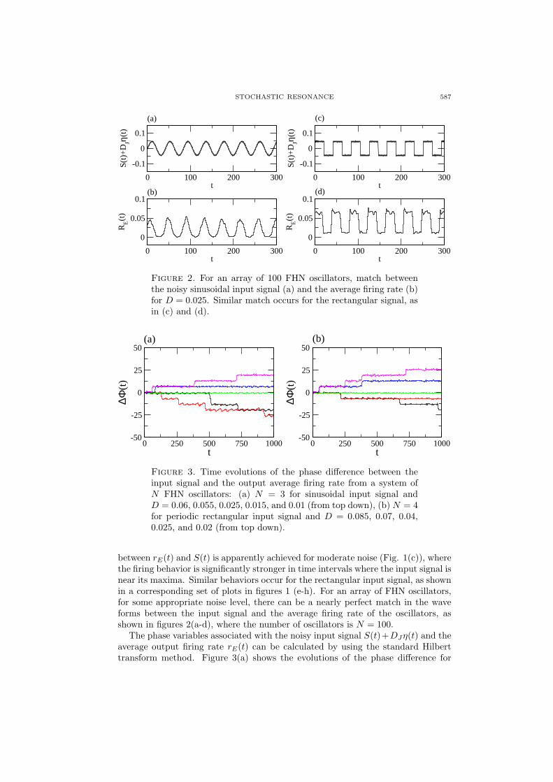
Figure 2. For an array of 100 FHN oscillators, match betweenthe noisy sinusoidal input signal (a) and the average firing rate (b)for D = 0.025. Similar match occurs for the rectangular signal, asin (c) and (d).

0 250 500 750 1000t

-50

-25

0

25

50

∆Φ(t

)

0 250 500 750 1000t

-50

-25

0

25

50

∆Φ(t

)

(a) (b)

Figure 3. Time evolutions of the phase difference between theinput signal and the output average firing rate from a system ofN FHN oscillators: (a) N = 3 for sinusoidal input signal andD = 0.06, 0.055, 0.025, 0.015, and 0.01 (from top down), (b) N = 4for periodic rectangular input signal and D = 0.085, 0.07, 0.04,0.025, and 0.02 (from top down).

between rE(t) and S(t) is apparently achieved for moderate noise (Fig. 1(c)), wherethe firing behavior is significantly stronger in time intervals where the input signal isnear its maxima. Similar behaviors occur for the rectangular input signal, as shownin a corresponding set of plots in figures 1 (e-h). For an array of FHN oscillators,for some appropriate noise level, there can be a nearly perfect match in the waveforms between the input signal and the average firing rate of the oscillators, asshown in figures 2(a-d), where the number of oscillators is N = 100.

The phase variables associated with the noisy input signal S(t)+DJη(t) and theaverage output firing rate rE(t) can be calculated by using the standard Hilberttransform method. Figure 3(a) shows the evolutions of the phase difference for


0 0.03 0.06 0.09 0.12D

0

500

1000

1500

2000τ

0 0.03 0.06 0.09 0.12D

0

500

1000

1500

2000

2500

τ

(a) (b)

Figure 4. Cusp-like behavior in the average phase-synchronization time about the optimal noise level: (a) forN = 3 and sinusoidal input signal, and (b) for N = 4 and periodicrectangular input signal. The synchronization times are expressedin units of the periods of the respective input signals.

five values of the internal noise amplitude: D = 0.06, 0.055, 0.025, 0.015, and 0.01(from top down), where the number of FHN oscillators is N = 3 and the inputis the sinusoidal signal. In the time interval used, no 2π phase slips occur whenthe noise is near the optimal level Dopt ≈ 0.025 (the middle trace). Such phaseslips occur and become relatively more frequent as D is away from Dopt. Similarbehavior is observed for the rectangular input signal, as shown in figure 3(b). Thecorresponding behaviors of the average synchronization time versus D are shown infigure 4(a) and 4(b), respectively, where we observe an apparent cusp-like featurenear the optimal noise level.

3. Theory.

3.1. Reduction of FHN model to double-well potential system. Heuris-tically, the dynamics of a single FHN oscillator can be reduced to the motion ofa classical mechanical particle in a double-well potential system [17, 18, 19]. Forpedagogical purposes, we outline the major steps in the reduction process. Usingthe change of variables, x → x + 1/2 and y → y − b + 1/2, we can convert thedynamical equations for a single FHN oscillator to

εx = −x(x2 − 1/4)− y + A + S(t) + DJη(t),y = x− y + Dξ(t), (2)

where A ≡ b− 1/2. For ε ¿ 1, the time rate of change of x(t) is much greater thanthat of y(t) and, hence, x(t) and y(t) can be regarded as a fast and a slow variable,respectively. Using the approximation

y ≈ 0 or y(t) ≈ xf (t) + Dξ(t),


where xf (t) is a solution of the FHN system in the presence of signal S(t) but inthe absence of noise, we can simplify the x-equation as

εx = −x(x2 − 14)− xf (t) + A + S(t) + D′ζ(t), (3)

where D′ζ(t) ≡ DJη(t)−Dξ(t) represents the combined noise and D′ =√

D2J + D2

is its amplitude. We have

εx = −∂U(x, t)/∂x + D′ζ(t), (4)

where the time-dependent potential function is given by

U(x, t) = x4/4− x2/8 + [xf (t)−A− S(t)]x, (5)

which is a tilted double-well potential. The solution of the single FHN equationscan then be interpreted as describing the motion of a heavily damped particlein the potential, with time-dependent slope of tilting. A firing event in a singleFHN oscillator is equivalent to a crossing of the particle through the barrier. Theensemble-averaged firing rate 〈r(t)〉 is determined by the Kramers formula [48, 49].Using perturbative analyses for xf (t) and to find the locations of the local minimaof the potential well as well as the maximum of the barrier, one can obtain thefollowing ensemble-averaged firing rate [17, 18, 19]:

〈r(t)〉 ∼ exp {−23

√3[B3 − 3B2S(t)]ε/D′}, (6)

where B is a constant which is the “distance” of the system’s excitation level tothe threshold [17, 18, 19].

For the array of FHN oscillators in equation (1), the mean firing rate is the sameas the ensemble-averaged firing rate of a single FHN oscillator. Fluctuations of thefiring rate are determined by noise of the following form: DJη(t)+(D/N)

∑Ni=1 ξi(t),

which can be written as D′′ζ ′(t), where D′′ =√

D2J + D2/N and ζ ′(t) is also

a Gaussian random signal of zero mean and unit variance. Taking into accountrandom fluctuations in the ensemble-averaged firing rate, we have

rE(t) = 〈r(t)〉+ σ(D′′)κ(t), (7)

where σ(D′′) is positive and proportional to D′′, and κ(t) is a Gaussian randomsignal.

3.2. Theoretical formulas of τ(D) for the double-well potential system.We now consider particle motion in an idealized double-well potential in the pres-ence of external driving and noise, subject to strong damping. The Langevin equa-tion can be written as

dx/dt = −dU(x)/dx + F (t) +√

2Dξ(t), (8)

whereU(x) = −x2/2 + x4/4, (9)

is the potential function, D is the noise amplitude, and ξ(t) is the white noise termthat satisfies 〈ξ(t)〉 = 0 and 〈ξ(t)ξ(t′)〉 = δ(t− t′). The potential has two wells, oneat xl = −1 and another at xr = 1, and a barrier at x = 0. To make analysis feasible,we consider the case where the external driving F (t) is a periodically rectangularsignal of period T0 = 1,

F (t) = { −F0 for 0 ≤ t < 1/2F0 for 1/2 ≤ t < 1.

(10)


Ed

E s

External forcing

First half−period Second half−period

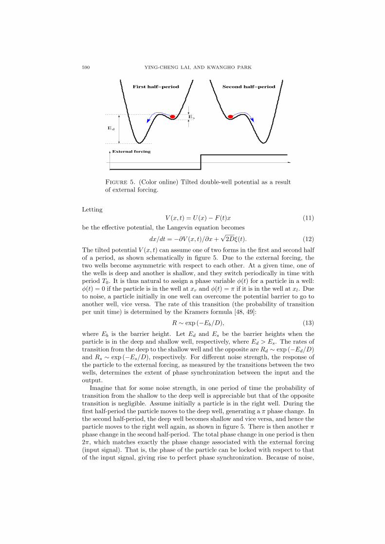
Figure 5. (Color online) Tilted double-well potential as a resultof external forcing.

LettingV (x, t) = U(x)− F (t)x (11)

be the effective potential, the Langevin equation becomes

dx/dt = −∂V (x, t)/∂x +√

2Dξ(t). (12)

The tilted potential V (x, t) can assume one of two forms in the first and second halfof a period, as shown schematically in figure 5. Due to the external forcing, thetwo wells become asymmetric with respect to each other. At a given time, one ofthe wells is deep and another is shallow, and they switch periodically in time withperiod T0. It is thus natural to assign a phase variable φ(t) for a particle in a well:φ(t) = 0 if the particle is in the well at xr and φ(t) = π if it is in the well at xl. Dueto noise, a particle initially in one well can overcome the potential barrier to go toanother well, vice versa. The rate of this transition (the probability of transitionper unit time) is determined by the Kramers formula [48, 49]:

R ∼ exp (−Eb/D), (13)

where Eb is the barrier height. Let Ed and Es be the barrier heights when theparticle is in the deep and shallow well, respectively, where Ed > Es. The rates oftransition from the deep to the shallow well and the opposite are Rd ∼ exp (−Ed/D)and Rs ∼ exp (−Es/D), respectively. For different noise strength, the response ofthe particle to the external forcing, as measured by the transitions between the twowells, determines the extent of phase synchronization between the input and theoutput.

Imagine that for some noise strength, in one period of time the probability oftransition from the shallow to the deep well is appreciable but that of the oppositetransition is negligible. Assume initially a particle is in the right well. During thefirst half-period the particle moves to the deep well, generating a π phase change. Inthe second half-period, the deep well becomes shallow and vice versa, and hence theparticle moves to the right well again, as shown in figure 5. There is then another πphase change in the second half-period. The total phase change in one period is then2π, which matches exactly the phase change associated with the external forcing(input signal). That is, the phase of the particle can be locked with respect to thatof the input signal, giving rise to perfect phase synchronization. Because of noise,


E

E s

d

OK

Figure 6. (color online) For D < Dopt, transition from the shal-low to the deep well can occur but the opposite is unlikely.

such a perfect synchronization cannot be achieved indefinitely. Let Dopt be thenoise amplitude for which the average synchronization time reaches a maximumvalue τmax À 1. Let Ψ2π(D) be the probability for a 2π change in one drivingperiod. We have

Ψ2π(Dopt) ≈ 1/τmax ≡ δ. (14)

Consider first the case D < Dopt. In the extreme case where D ≈ 0, the Kramersrates are essentially zero so that a particle initially in one potential well will remainthere for a long time. Due to the 2π phase change in the input signal in one period,there will be a corresponding 2π change in the phase difference ∆φ between theinput and the output signal. We have Ψ2π(0) ≈ 1. As D is increased from zero, itbecomes possible for a particle in the shallow well to move to the deep well so thatRs will increase, but if D is small, we expect Rd to remain negligible because of thehigher potential barrier, as shown in figure 6. This will reduce Ψ2π(D) from unity.The amount of reduction is given by the Kramers rate Rs. The probability for 2πphase change is thus (1 − C0Rs), where C0 is a constant that can be determinedby the condition Ψ2π(Dopt) ≈ δ. We obtain

Ψ<2π(D) = 1− (1− δ) exp (Es/Dopt) exp (−Es/D). (15)

The average phase synchronization time for D < Dopt is given by τ<(D) ≈ 1/Ψ<2π(D).

We have

dτ<(D)/dD|D→D−opt≈ (1− δ)Es

δ2D2opt

(16)

anddτ<(D)/dD|D→D−

opt→∞, for ε → 0.


E

E s

d

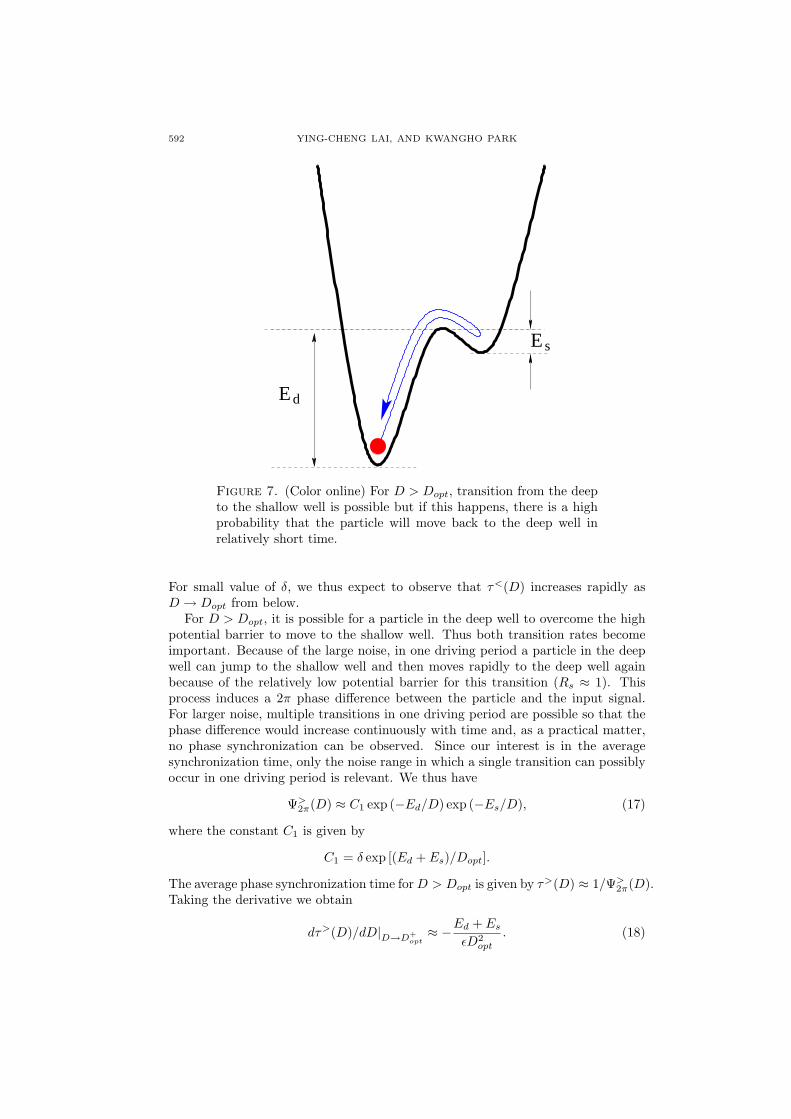
Figure 7. (Color online) For D > Dopt, transition from the deepto the shallow well is possible but if this happens, there is a highprobability that the particle will move back to the deep well inrelatively short time.

For small value of δ, we thus expect to observe that τ<(D) increases rapidly asD → Dopt from below.

For D > Dopt, it is possible for a particle in the deep well to overcome the highpotential barrier to move to the shallow well. Thus both transition rates becomeimportant. Because of the large noise, in one driving period a particle in the deepwell can jump to the shallow well and then moves rapidly to the deep well againbecause of the relatively low potential barrier for this transition (Rs ≈ 1). Thisprocess induces a 2π phase difference between the particle and the input signal.For larger noise, multiple transitions in one driving period are possible so that thephase difference would increase continuously with time and, as a practical matter,no phase synchronization can be observed. Since our interest is in the averagesynchronization time, only the noise range in which a single transition can possiblyoccur in one driving period is relevant. We thus have

Ψ>2π(D) ≈ C1 exp (−Ed/D) exp (−Es/D), (17)

where the constant C1 is given by

C1 = δ exp [(Ed + Es)/Dopt].

The average phase synchronization time for D > Dopt is given by τ>(D) ≈ 1/Ψ>2π(D).

Taking the derivative we obtain

dτ>(D)/dD|D→D+opt≈ −Ed + Es

εD2opt

. (18)


Again we observe that

|dτ>(D)/dD|D→D+opt→∞ for ε → 0.

Equations (16) and (18) thus indicate a cusp-like behavior in τ(D) about Dopt.Moreover, we have

dτ<(D)/dD|D→D−opt6= |dτ>(D)/dD|D→D+

opt. (19)

For small value of δ, for D → D−opt, the rise of τ<(D) can be pronounced than

that of τ>(D) for D → D+opt. In general, we expect to see an asymmetric behavior

in τ(D) near Dopt. Note also that equation (17) implies that for D > Dopt, theaverage time τ>(D) obeys the following scaling law with the noise amplitude:

τ>(D) ∼ exp [(Ed + Es)/D]. (20)

We emphasize that equations (16) and (18) indicate a fast rising and a fastfalling behavior in the average synchronization time only for noise amplitude belowand above the optimal value, respectively. Our argument is not applicable whenthe noise amplitude is in the infinitesimal vicinity of the optimal value. Thus, ourheuristic theory cannot predict whether there is a cusp behavior in the mathematicalsense of discontinuity in the derivative. A recent analytic expression [50, 51] for theinstantaneous phase-diffusion coefficient in a periodically driven system suggests,however, a smooth behavior in the phase-synchronization time about the optimalnoise level. In particular, the diffusion coefficient shows a sharp but smooth peak atthe optimal noise level. Since the average phase-synchronization time can be relatedto the inverse of the diffusion coefficient [52], it is reasonable that the behavior ofthis time also be smooth.

4. Numerical results with the double-well system. Here we present numeri-cal support for the cusp-like behavior in the double-well system with both periodicrectangular and sinusoidal driving.

4.1. Periodic rectangular driving. By examining the average synchronizationtime, the optimal noise amplitude is determined to be Dopt ≈ 0.033. Figures 8(a-c) show, for driving amplitude F0 = 0.18, the output signal x(t) with respect tothe input for three values of the noise amplitude. For D = 0.02 < Dopt (a), thereare infrequent mismatches between the phases. For D = 0.033 ≈ Dopt, we observealmost a perfect phase match between the input and the output signal in the timeinterval displayed. For D = 0.1 > Dopt, phase mismatches occur quite often. Thesesuggest that noise of amplitude D near Dopt results in a maximal degree of phasesynchronization between the input and the output signal.

Figure 9 shows, for the same driving amplitude, evolutions of the phase differencebetween the input and the output signal. Here the phase variable associated withthe output is defined to be

φout(t) = tan−1 x(t)x(t)

,

where x(t) is the Hilbert transform of x(t):

x(t) = P.V.

[1π

∫ ∞

−∞

x(t′)t− t′

dt′]

,

and P.V. stands for the Cauchy principal value for integral. The five traces shownfrom top down correspond to D = 0.041, D = 0.038, D = 0.033 ≈ Dopt, D = 0.028,


-2

-1

0

1

2

-2

-1

0

1

2

x(t)

, F(

t)

0 5 10t/T

0

-2

-1

0

1

2

Figure 8. (Color online) For the double-well potential system un-der periodic rectangular driving of amplitude F0 = 0.18, the outputsignal x(t) in relation to the input driving for three values of thenoise amplitude: (a) D = 0.02 < Dopt, (b) D = 0.033 ≈ Dopt, and(c) D = 0.1 > Dopt.

0 100 200 300 400 500 600t/T

0

-40

-20

0

20

40

∆Φ(t

)

Figure 9. (Color online) For the double-well potential system un-der periodic rectangular driving of amplitude F0 = 0.18, evolutionsof the phase difference between the input and the output for fivedifferent values of the noise amplitude.


0 0.02 0.04 0.06 0.08D

0

5000

10000

15000

20000

τ

0.025 0.03 0.035 0.04D

0

5000

10000

15000

20000

τ

(a) (b)

Figure 10. (Color online) For the double-well potential systemunder periodic rectangular driving, (a) cusp-like behavior in thedependence of the average phase-synchronization time on noiseamplitude, (b) asymmetric behavior of this dependence about theoptimal noise amplitude.

and D = 0.025, respectively. Within the time considered (600 driving periods),we observe 2π phase slips for all noise levels except for D = 0.033, indicatingthat relatively long phase synchronization has been achieved and, hence, this isapproximately the optimal noise amplitude, which has been observed to yield amaximum in the SNR. In this sense the measure of average phase-synchronizationtime is consistent with the traditional measures for characterizing SR. As D deviatesaway from Dopt, 2π phase slips occur more often.

To verify the cusp-like behavior in the average phase-synchronization time τ , wechoose a number of values of the noise amplitude about Dopt. For each value, weuse 20 realizations of the stochastic system to calculate the average value of thetime between successive 2π phase slips. The result is shown in figure 10 (a), wherewe see that τ exhibits apparently a cusp-like behavior about the optimal noiseamplitude Dopt. As the noise amplitude is increased from zero and approachesthe optimal value, there are four orders of magnitude of increase in the averagephase-synchronization time, indicating an extremely high sensitivity to noise ascompared with the traditional measures. The asymmetric behavior in τ aboutDopt, as predicted by our theoretical analysis, is shown in figure 10 (b), which isa blowup of part of figure 10 (a) near Dopt. Support for the predicted scaling law(20) for D > Dopt is shown in figure 11.

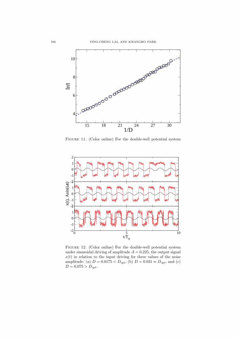
4.2. Sinusoidal driving. We have obtained similar results when the input drivingis a smooth sinusoidal signal A sin t. In particular, figures 12 (a-c) show, for A =0.225, the output signal x(t) in relation to the input for three values of the noiseamplitude: (a) D = 0.0175 < Dopt, (b) D = 0.031 ≈ Dopt, and (c) D = 0.075 >Dopt. We see nearly perfect phase match between the input and the output signalfor D ≈ Dopt (panel (b)). Figure 13 shows the evolutions of the phase differencebetween the input and the output signal for five different values of noise level. The


15 18 21 24 27 301/D

4

6

8

10

lnτ

Figure 11. (Color online) For the double-well potential systemunder periodic rectangular driving, evidence for the scaling law(20).

-2

-1

0

1

2

-2

-1

0

1

2

x(t)

, Asi

n(ω

t)

0 5 10t/T

0

-2

-1

0

1

2

Figure 12. (Color online) For the double-well potential systemunder sinusoidal driving of amplitude A = 0.225, the output signalx(t) in relation to the input driving for three values of the noiseamplitude: (a) D = 0.0175 < Dopt, (b) D = 0.031 ≈ Dopt, and (c)D = 0.075 > Dopt.


0 100 200 300 400 500t/T

0

-50

0

50

100

∆Φ(t

)

Figure 13. (Color online) For the double-well potential systemunder sinusoidal driving of amplitude A = 0.225, evolutions ofthe phase difference between the input and output for D = 0.04,D = 0.035, D = 0.031 ≈ Dopt, D = 0.025, and D = 0.0225 (top tobottom).

0.0225 0.03 0.0375 0.045 0.0525D

0

3000

6000

9000

12000

τ

Figure 14. (Color online) For the double-well potential systemunder sinusoidal driving, cusp-like behavior in the dependence ofthe average phase-synchronization time on noise amplitude.


0 0.002 0.004 0.006 0.008 0.01ω

0

3000

6000

9000

12000

15000

τ

Figure 15. (Color online) For the double-well potential systemunder sinusoidal driving, cusp-like behavior in the dependence ofthe average phase-synchronization time on the frequency of theexternal driving signal (bona-fide stochastic resonance).

nearly horizontal trace without large steps correspond to the case of D ≈ Dopt. Thecusp-like behavior in the average phase-synchronization time is shown in figure 14.

The cusp-like behavior in the average phase-synchronization time can also occurwith respect to variation in the frequency of the external signal, the so-called bona-fide stochastic-resonance phenomenon [53, 54, 55]. To demonstrate this, we fixD = 0.031 ≈ Dopt and calculate the average synchronization time τ as a function ofthe frequency of the input signal. The result is shown in figure 15, where τ exhibitsa similar cusp-like behavior as in figures 10 and 14. Thus, the synchronization timeis sensitive not only to noise variation, but also to other parameters such as thefrequency of the driving signal. This may be interesting from the standpoint offrequency tuning in biological systems or in device applications.

5. Discussion. Characterization of SR by using the phase-synchronization timemay be of fundamental interest because this represents an alternative way to studySR. This approach can also be practically useful because the synchronization timedepends on the noise level much more sensitively than the traditional measures suchas the SNR. This may provide insights into the mechanism for biological systemsto tune noise to achieve optimal performance through SR. In terms of technologicalapplications, suppose an instrument is to be built based on the phenomenon of SR.Using this time measure can be more advantageous because of the higher precisionit can potentially offer. In this paper, we have presented numerical evidence for thehigh noise sensitivity in a paradigmatic model of biological oscillators. To be ableto obtain analytic understanding, we have used the standard double-well potentialmodel with a periodic input signal. The dynamics of phase synchronization is thenanalyzed based on the transitions between the potential wells, with the help of theKramers formula. Our principal finding is that, near the optimal noise level, the


function τ(D) exhibits a cusp-like maximum with distinct values of derivative de-pending on whether the optimal level is approached from below or above. Althoughthe specifics of τ(D) depend on the details of the system and the input signal, ouranalysis and numerical computations indicate that the cusp-like behavior is general.While our analysis is heuristic, a more rigorous treatment may be possible using arecently proposed two-state, discrete phase model for SR [36, 37]. Although thereis a huge body of literature on SR, to our knowledge, the cusp-like behavior in thesynchronization time has not been noticed previously.

Our approach to understanding stochastic resonance may also be useful for thephenomenon of resonant activation [56, 57, 58, 59] where, for a particle in a potentialwell with a time-varying barrier, in the presence of noise the average crossing time,which is the average of times required to diffuse over each of barriers, can exhibit aminimum as a parameter controlling the barrier height varies. In previous works,the reported resonance peak is typically broad [56, 57, 58, 59]. Our results hereimply that if resonant activation is treated using phase synchronization, it is possiblethat the average synchronization time can exhibit a cusp-like, sharp maximum. Apossible setting to establish this is to assume that the barrier height is controlledby a time-varying signal (e.g., chaotic) for which a phase variable can be defined.The relative phase difference between the particle and this signal, and consequentlyphase synchronization, can then be investigated as in this paper.

Acknowledgments. We thank Dr. A. Nachman for stimulating discussions aboutstochastic resonance and applications, which motivated the present work. We alsothank professors P. Hanggi, L. Schimansky-Geier, F. Marchesoni, Manuel Morillo,and J. M. Rubi for their insights and discussions. This work was supported byAFOSR under Grants No. F49620-03-1-0290 and No. FA9550-06-1-0024.

REFERENCES

[1] A. Longtin, A. Bulsara, and F. Moss, Time-interval sequences in bistable systems andthe noise-induced transmission of information by sensory neurons. Phys. Rev. Lett.67 (1991) 656-659.

[2] K. Wiesenfeld, D. Pierson, E. Pantazelou, C. Dames, and F. Moss, Stochastic resonanceon a circle. Phys. Rev. Lett. 72 (1994) 2125-2129.

[3] P. C. Gailey, A. Neiman, J. J. Collins, and F. Moss, Stochastic resonance in ensemblesof nondynamical elements: the role of internal noise. Phys. Rev. Lett. 79 (1997)4701-4704.

[4] J. K. Douglass, L. Wilkens, E. Pantazelou, and F. Moss, Noise enhancement of informa-tion transfer in crayfish mechanoreceptors by stochastic resonance. Nature (Lon-don) 365 (1993) 337-340.

[5] J. E. Levin and J. P. Miller, Broadband neural encoding in the cricket cereal sensorysystem enhanced by stochastic resonance. Nature (London) 380 (1996) 165-168.

[6] J. J. Collins, T. T. Imhoff, and P. Grigg, Noise-enhanced information transmission inrat SA1 cutaneous mechanoreceptors via aperiodic stochastic resonance. J. Neuro-physiol. 76 (1996) 642-645.

[7] R. P. Morse and E. F. Evans, Enhancement of vowel coding for cochlea implants byaddition of noise. Nature Medicine 2 (1996) 928-932.

[8] P. Cordo, J. T. Inglis, S. Verschueren, J. J. Collins, D. M. Merfeld, S. Rosenblum, S. Buckley,and F. Moss, Noise in human muscle spindles. Nature (London) 383 (1996) 769-770.

[9] B. J. Gluckman, T. I. Netoff, E. J. Neel, W. L. Ditto, M. L. Spano, and S. J. Schiff, Stochas-tic Resonance in a Neuronal Network from Mammalian Brain. Phys. Rev. Lett. 77(1996) 4098-4101.

[10] P. E. Greenwood, L. M. Ward, D. F. Russell, A. Neiman, and F. Moss, Stochastic reso-nance enhances the electrosensory information available to paddlefish for preycapture. Phys. Rev. Lett. 84 (2000) 4773-4776.


[11] E. Simonotto, M. Riani, C. Seife, M. Roberts, J. Twitty, F. Moss, Visual perception ofstochastic resonance. Phys. Rev. Lett. 78 (1997) 1186-1189.

[12] R. Benzi, A. Sutera, and A. Vulpiani, The mechanism of stochastic resonance. J. Phys.A 14 (1981) L453-L457.

[13] R. Benzi, G. Parisi, A. Sutera, and A. Vulpiani, A theory of stochastic resonance inclimatic change. SIAM J. Appl. Math. 43 (1983) 565-578.

[14] K. Wiesenfeld and F. Moss, Stochastic resonance and the benefits of noise: from iceages to crayfish and SQUIDs. Nature (London) 373 (1995) 33-36.

[15] L. Gammaitoni, P. Hanggi, P. Jung, and F. Marchesoni, Stochastic resonance. Rev. Mod.Phys. 70 (1998) 223-287.

[16] B. McNamara, K. Wiesenfeld, and R. Roy, Observation of Stochastic Resonance in aRing Laser. Phys. Rev. Lett. 60 (1988) 2626-2629.

[17] J. J. Collins, C. C. Chow, and T. T. Imhoff, Stochastic resonance without tuning.Nature 376 (1995) 236-238.

[18] J. J. Collins, C. C. Chow, and T. T. Imhoff, Aperiodic stochastic resonance in excitablesystems. Phys. Rev. E 52 (1995) R3321-R3324.

[19] J. J. Collins, C. C. Chow, A. C. Capela, and T. T. Imhoff, Aperiodic stochastic resonance.Phys. Rev. E 54 (1996) 5575-5584.

[20] M. E. Inchiosa and A. R. Bulsara, Nonlinear dynamic elements with noisy sinusoidalforcing: Enhancing response via nonlinear coupling. Phys. Rev. E 52 (1995) 327-339.

[21] M. E. Inchiosa, A. R. Bulsara, A. D. Hibbs, and B. R. Whitecotton, Signal Enhancementin a Nonlinear Transfer Characteristic. Phys. Rev. Lett. 80 (1998) 1381-1384.

[22] M. E. Inchiosa, A. R. Bulsara, A. D. Hibbs, and B. R. Whitecotton, Signal Enhancementin a Nonlinear Transfer Characteristic Phys. Rev. Lett. 80 (1998) 1381-1384.

[23] Hanggi, M. E. Inchiosa, D. Fogliatti, and A. R. Bulsara, Nonlinear stochastic resonance:The saga of anomalous output-input gain. Phys. Rev. E 62 (2000) 6155-6163.

[24] N. G. Stocks, Suprathreshold Stochastic Resonance in Multilevel Threshold Sys-tems. Phys. Rev. Lett. 84 (2000) 2310-2313.

[25] N. G. Stocks and R. Mannella, Generic noise-enhanced coding in neuronal arrays.Phys. Rev. E 64 (2001) 030902.

[26] B. Ando, S. Baglio, S. Graziani, and N. Pitrone, An Instrument for the Detection ofOptimal Working Conditions in Stochastic Systems. Int. J. Electron. 86 (1999) 791-806.

[27] B. Ando and S. Graziani, Noise tuning in stochastic systems. Int. J. Electron. 87 (2000)659-666.

[28] B. Ando, S. Baglio, S. Graziani, and N. Pitrone, Measurements of parameters influenc-ing the optimal noise level in stochastic systems. IEEE Trans. Instru. Meas. 49 (2000)1137-1143

[29] B. Ando and S. Graziani, An instrument for the detection of optimal working con-ditions in stochastic systems. IEEE Trans. Instru. Meas. 52 (2000) 815-821.

[30] B. Shulgin, A. Neiman, and V. Anishchenko, Mean Switching Frequency Locking inStochastic Bistable Systems Driven by a Periodic Force. Phys. Rev. Lett. 75 (1995)4157-4160.

[31] F. Marchesoni, F. Apostolico, and S. Santucci, Switch-phase distributions and stochasticresonance. Phys. Lett. A 248 (1998) 332-337.

[32] A. Neiman, A. Silchenko, V. Anishchenko, and L. Schimansky-Geier, Stochastic reso-nance: Noise-enhanced phase coherence. Phys. Rev. E 58 (1998) 7118-7125.

[33] J. A. Freund, L. Schimansky-Geier, and P. Hanggi, Frequency and phase synchronizationin stochastic systems. Chaos 13 (2003) 225-238.

[34] J. A. Freund, A. B. Neiman, and L. Schimansky-Geiger, Analytic description of noise-induced phase synchronization. Europhys. Lett. 50 (2000) 8-14.

[35] R. Rozenfeld, J. A. Freund, A. Neiman, and L. Schimansky-Geiger, Noise-induced phasesynchronization enhanced by dichotomic noise. Phys. Rev. E 64 (2001) 051107.

[36] L. Callenbach, P. Hanggi, S. J. Linz, J. A. Freund, and L. Schimansky-Geier, Oscillatorysystems driven by noise: Frequency and phase synchronization. Phys. Rev. E 65 (2002)051110.

[37] B. Lindner, J. Garcia-Ojalvo, A. Neiman, L. Schimansky-Geier, Effects of noise in ex-citable systems. Phys. Rep. 392 (2004) 321-424.

[38] A. Longtin and D. R. Chialvo, Stochastic and Deterministic Resonances for ExcitableSystems. Phys. Rev. Lett. 81 (1998) 4012-4015.


[39] F. Marino, M. Giudici, S. Barland, and S. Balle, Experimental Evidence of StochasticResonance in an Excitable Optical System. Phys. Rev. Lett. 88 (2002) 040601.

[40] K. Park, Y.-C. Lai, Z. Liu, and A. Nachman, Aperiodic stochastic resonance and phasesynchronization. Phys. Lett. A 326 (2004) 391-396.

[41] M. G. Rosenblum, A. S. Pikovsky, and J. Kurths, Phase Synchronization of ChaoticOscillators. Phys. Rev. Lett. 76 (1996) 1804-1807.

[42] Perfect synchronization in the phase defined by ∆φ(t) = 0 can be achieved only when completesynchronization between the dynamical variables of the coupled oscillators occurs, whichusually requires strong coupling [41]. Phase synchronization in this case may be trivial becausecomplete synchronization represents the ultimate synchronous state that a system of coupledoscillators can achieve. Phase synchronization is interesting in the weakly coupling regime,where complete synchronization has not set in and the amplitudes of the coupled oscillatorsremain uncorrelated. To better see this, consider the simple case of a coupled system of tworotors with slightly different frequencies. When the coupling is zero, on average the phasedifference increases monotonically with time because of the small difference in frequency,but, with a small amount of coupling, the frequencies can become entrained and the phasedifference can remain bounded. The disappearance of the monotonic growth of the phasedifference signifies the onset of phase coherence. That is why the standard definition of phasesynchronization [41, 43] is ∆φ(t) < 2π for all t.

[43] A. Pikovsky, M. Rosenblum, and J. Kurths, Synchronization - A Universal Concept inNonlinear Sciences. Cambridge Univ. Press, Cambridge, UK, 2001.

[44] K. Park and Y.-C. Lai, Characterization of stochastic resonance. Europhys. Lett. 70(2005) 432-438.

[45] R. A. FitzHugh, Impulses and physiological states in theoretical models of nervemembrane. Biophys. J. 1 (1961) 445-466.

[46] A. C. Scott, The electrophysics of a nerve fiber. Rev. Mod. Phys. 47 (1975) 487-533.[47] P. E. Kloeden and E. Platen, Numerical Solution of Stochastic Differential Equa-

tions. Springer-Verlag, Berlin, 1992.[48] H. A. Kramers, Brownian motion in a field of force and the diffusion model of

chemical reactions. Physica (Utrecht) 7 (1940) 284-304.[49] P. Hanggi, P. Talkner, and M. Borkovec, Reaction-rate theory: fifty years after

Kramers. Rev. Mod. Phys. 62 (1990) 251-341.[50] J. Casado-Pascual, J. Gomez-Ordonez, M. Morillo, J. Lehmann, I. Goychuk, and P. Hanggi,

Theory of frequency and phase synchronization in a rocked bistable stochasticsystem. Phys. Rev. E 71 (2005) 011101.

[51] T. Prager and L. Schimansky-Geier, Phase velocity and phase diffusion in periodicallydriven discrete-state systems. Phys. Rev. E 71 (2005) 031112.

[52] V. S. Anishchenko, V. V. Astakhov, A. B. Neiman, T. E. Vadivasova, and L. Schimansky-Geier, Nonlinear Dynamics of Chaotic and Stochastic Systems. Tutorial and Mod-ern Development. Springer, Berlin, 2002.

[53] L. Gammaitoni, F. Marchesoni, E. Menichella-Saetta, and S. Santucci, Resonant crossingprocesses controlled by colored noise. Phys. Rev. Lett. 71 (1993) 3625-3628.

[54] L. Gammaitoni, F. Marchesoni, and S. Santucci, Stochastic Resonance as a Bona FideResonance. Phys. Rev. Lett. 74 (1995) 1052-1055.

[55] S. Barbay, G. Giacomelli, and F. Marin, Stochastic resonance in vertical cavity surfaceemitting lasers. Phys. Rev. E 61 (2000) 157-166.

[56] C. R. Doering and J. C. Gadoua, Resonant activation over a fluctuating barrier.Phys. Rev. Lett. 69 (1992) 2318-2321.

[57] P. Pechukas and P. Hanggi, Rates of Activated Processes with Fluctuating Barriers.Phys. Rev. Lett. 73 (1994) 2772-2775.

[58] M. Marchi, F. Marchesoni, L. Gammaitoni, E. Menichella-Saetta, and S. Sautucci, Resonantactivation in a bistable system. Phys. Rev. E 54 (1996) 3479-3487.

[59] A. L. Pankratov and B. Spagnolo, Suppression of Timing Errors in Short OverdampedJosephson Junctions. Phys. Rev. Lett. 93 (2004) 177001.


Received on February 20, 2006. Accepted on March 28, 2006.

E-mail address: [email protected]

E-mail address: [email protected]

noise-sensitive measure for stochastic resonance...

Documents