Noise and adaptation in multistable perception: Noise driveswhen to switch, adaptation determines percept choice

Gemma Huguet # $Department of Applied Mathematics I, Universitat

Politecnica de Catalunya, Barcelona, Spain

John Rinzel # $

Center for Neural Science and Courant Institute ofMathematical Sciences, New York University, New York,

NY, USA

Jean-Michel Hupe # $

Centre de Recherche Cerveau et Cognition, ToulouseUniversity and Centre National de la Recherche

Scientifique, Toulouse, France

We study the dynamics of perceptual switching inambiguous visual scenes that admit more than twointerpretations/percepts to gain insight into thedynamics of perceptual multistability and its underlyingneural mechanisms. We focus on visual plaids that aretristable and we present both experimental andcomputational results. We develop a firing-rate modelbased on mutual inhibition and adaptation that involvesstochastic dynamics of multiple-attractor systems. Themodel can account for the dynamic properties (transitionprobabilities, distributions of percept durations, etc.)observed in the experiments. Noise and adaptation haveboth been shown to play roles in the dynamics ofbistable perception. Here, tristable perception allows usto specify the roles of noise and adaptation in ourmodel. Noise is critical in considering the time of aswitch. On the other hand, adaptation mechanisms arecritical in considering perceptual choice (in tristableperception, each time a percept ends, there is a possiblechoice between two new percepts).

Introduction

When observers view for an extended time anambiguous visual scene (admitting two or moredifferent interpretations), they report spontaneousswitching between different perceptions. Typical ex-amples of perceptual bistability (two interpretations)and spontaneous switching in visual perception includebinocular rivalry (alternation of two different images,one presented to each eye), ambiguous geometric

figures such as the Necker cube (alternation of twodepth organizations), ambiguous figure–ground segre-gation such as Rubin’s vase-face (alternation of twofigure–ground organizations), ambiguous motion dis-plays (alterations of two arrangements of movingobjects), and more (for reviews, see Leopold &Logothetis, 1999; Blake & Logothetis, 2002; Long &Toppino, 2004).

Experimental results (imaging in humans andelectrophysiology in monkeys) have revealed neuronalactivity that correlates with the subject’s perception inthe visual cortex as well as the parietal and frontalcortex (Leopold & Logothetis, 1999; Tong & Engel,2001; Sterzer & Kleinschmidt, 2007). Although theneuronal bases of perception for ambiguous stimuli arestill controversial (see Sterzer, Kleinschmidt, & Rees,2009, for a review), those observations inspired thecurrent formal models of multistability. The models tryto explain as much as possible of the variability ofperceptual dynamics with simple mechanisms thatcould be implemented in relatively low-level sensorysystems (like the visual cortex for visual multistability).

The existing models for perceptual multistabilityfocus on bistable rivalry (Lago-Fernandez & Deco,2002; Laing & Chow, 2002; Wilson, 2003; Moreno-Bote, Rinzel, & Rubin, 2007). In these models, themechanism underlying the alternating rhythmic be-havior involves competition between two neuronalpopulations (whose activity is correlated to a particularpercept) via reciprocal inhibition and some form ofslow adaptation or negative feedback acting on thedominant population (spike frequency adaptation and/

Citation: Huguet, G., Rinzel, J., & Hupe, J.-M. (2014). Noise and adaptation in multistable perception: Noise drives when toswitch, adaptation determines percept choice. Journal of Vision, 14(3):19, http://www.journalofvision.org/content/14/3/19,doi:10.1167/14.3.19.

Journal of Vision (2014) 14(3):19, 1–24 1http://www.journalofvision.org/content/14/3/19

doi: 10 .1167 /14 .3 .19 ISSN 1534-7362 � 2014 ARVOReceived July 8, 2013; published March 13, 2014

or synaptic depression). Noise is added to the system toaccount for the irregular oscillations and, in somemodels, to become the essential driving force for theswitching mechanism (Moreno-Bote et al., 2007;Shpiro, Moreno-Bote, Rubin, & Rinzel, 2009).

The roles of slow adaptation and neuronal noise inbistable rivalry have been extensively studied. It iswidely accepted that both elements are involved inrivalry; the discussion focuses on the balance betweenthe two (Brascamp, van Ee, Noest, Jacobs, & van denBerg, 2006; Moreno-Bote et al., 2007; Shpiro et al.,2009). In oscillatory models, slow adaptation isultimately responsible for alternations, while in noise-driven attractor models, noise drives switching in awinner-take-all framework. To assess the roles of noiseand adaptation, the models try to conform toexperimental data on dominance durations (averages,histogram shapes, correlations between successivedurations, etc.) and some well-known principles ofbinocular rivalry known as Levelt’s propositions,especially Propositions 2 and 4 (Levelt, 1968). Forthose models, the system should operate near theboundary between being adaptation driven and noisedriven (Shpiro et al., 2009; Pastukhov et al., 2013).Here we study tristability to further constrain thesemodels, and we find that adaptation and noise not onlyare both important but also play different roles.

Though the dynamics of bistable rivalry have beenextensively studied, attempts to generalize these modelsto stimuli with more than two competing percepts arescarce in the literature. However, unlike in bistablerivalry, where only temporal patterns are informative,in multistable rivalry with more than two percepts,differential transition patterns provide more insightinto the plausible mechanisms that generate perceptualmultistability (Burton, 2002; Suzuki & Grabowecky,2002; Naber, Gruenhage, & Einhauser, 2010; Wallis &Ringelhan, 2013). Moreover, given that sensory infor-mation can have multiple interpretations, moving frombistability to multistability is a necessary step inachieving understanding about how the brain dealswith ambiguity.

To study multistable rivalry, we focus on a classicalparadigmatic stimulus, called visual plaids, consistingof two superimposed drifting gratings (Wallach, 1935;Hupe & Rubin, 2003; for a demonstration, visit http://cerco.ups-tlse.fr/;hupe/plaid_demo/demo_plaids.html). With visual plaids, tristable perception isexperienced (see Figure 1): one coherent or integratedpercept (the gratings moving together as a singlepattern) and two transparent or segregated percepts(the gratings sliding across one another) with alternat-ing depth order (which grating is perceived asforeground and which as background; Rubin & Hupe,2005; Moreno-Bote, Shpiro, Rinzel, & Rubin, 2008;Naber et al., 2010; Hupe & Pressnitzer, 2012).

Here we present experimental data from psycho-physics on tristable plaids and a computational modelthat specifies quantitatively current hypotheses ofperceptual switching to reproduce experimental obser-vations.

For bistable stimuli, the effects of varying parame-ters of the stimulus are typically described by thechanges on the dominance durations (the period oftime a percept stays active). But for tristable stimuli,one can also look at the effect on percept probabilities(fraction of percept occurrences) and their relation todominance durations (Naber et al., 2010). In the case ofvisual plaids, there are several parameters of thestimulus that can be modified: speed, spatial frequency,contrast, directions of motion, and so on (Adelson &Movshon, 1982; Hupe & Rubin, 2003; Moreno-Bote,Shpiro, Rinzel, & Rubin, 2008; Hedges, Stocker, &Simoncelli, 2011). In this study, we investigated ahighly constrained set of parameter conditions—onlythree stimuli (corresponding to three different values ofthe angle a between the normal vectors to the gratings)and a single motion direction (see Figure 1)—butrepeated many times, in order to gather for each subjectenough perceptual sequences collected within the exactsame conditions. In agreement with previous experi-ments (Naber et al., 2010), we observe that changes in a

Figure 1. (A) Visual plaids consist of two superimposed gratings

whose normal vectors differ by an angle a (VP). Representation

of different interpretations for visual plaids: coherent motion

(C) and transparent motion (T). Transparent motion is

ambiguous with respect to depth ordering and admits two

different interpretations: with the grating moving to the left

perceived on top (TL) and with the grating moving to the right

perceived on top (TR). (B) Tristability refers to coherent (C),

transparent left (TL), and transparent right (TR) percepts, which

we identify with the colors red, blue, and green, respectively.

Journal of Vision (2014) 14(3):19, 1–24 Huguet, Rinzel, & Hupe 2

produce changes in both dominance durations andpercept probabilities.

By examining triplets consisting of two transparentpercepts interleaved with a coherent one, we find thatthe next percept probability depends on the durationsof the current and the previous percept. Theserelationships are newfound with respect to bistablestimuli, where correlations could be measured onlybetween dominance durations. These correlations werereported as absent or insignificant for bistability(although see, for example, van Ee, 2009; Pastukhov &Braun, 2011), as we also find for our tristable stimuli.Thus, our results showing that percept choice but notpercept duration depends on recent perceptual historysuggest that adaptation and noise are involved indifferent aspects of perceptual switching.

We test the roles of adaptation and noise in acomputational model that is based on the firing-ratemodels for alternations in perceptual bistability (Laing& Chow, 2002; Moreno-Bote et al., 2007). Our modelconsists of three mutually coupled populations of cells,each one encoding a different percept. We proposeinhibition-based competition along with adaptationand noise as plausible mechanisms for the dynamics ofperceptual switching. Importantly, optimal parametersare obtained for a noise-driven regime, suggesting thatnoise is the ultimate cause of perceptual switching.However, slow adaptation, in particular subtractiveadaptation, is essential in accounting for the decrease inthe probability of a switch back after a short duration,suggesting that adaptation is important for perceptualchoice.

Methods

Psychophysical experiment

Observers

Nine observers participated in the experiment. Theyhad normal or corrected-to-normal eyesight and gaveinformed consent for their participation. Data arepresented for eight subjects (see ‘‘Data analysis’’ later;average age¼26, range¼ [20, 46]; four women and fourmen).

Apparatus

We presented stimuli on a 21-in. Sony TrinitronGDM-F520 monitor (30.4 cm vertical viewable screensize) at a frame rate of 85 Hz. The screen resolution was1600·1200 pixels. Subjects were comfortably seated 57cm in front of the screen in a dimly lit room, with theirchin and forehead resting on a chinrest (University ofHouston College of Optometry, Houston, TX). Two

small cameras were attached to the chinrest just abovethe eyes and looked at the eyes through semitranspar-ent mirrors. Eye position (difference between the pupiland corneal reflection centers) and pupil diameter wererecorded binocularly at 240 Hz by using an ISCANETL-200 system (Burlington, MA). The experimenter(Marie Fellmann, as training for her first-year master’sthesis) was present in the room to verify the quality ofthe eye signals. Off-line visual inspection of eyepositions revealed that all subjects were maintainingaccurate fixation.

Stimuli

The stimuli comprised two rectangular-wave grat-ings presented through a circular aperture 68 in radius.The luminance of the gray surround was 24 cd/m2 (20%of the maximal luminance of the screen). The gratingscomprised thin dark stripes (14 cd/m2, duty cycle¼ 0.3,spatial frequency¼ 0.3 c/8) on a lighter background (28cd/m2) and appeared as figures moving over thebackground. The intersecting regions were darker thanthe gratings (11 cd/m2, in the middle of the transpar-ency range). Which grating was in front was ambigu-ous. Gratings moved at 1.58/s (measured in thedirection normal to their orientation) in directions 808,1008, and 1208 apart (angle a hereafter). The patternwas moving upwards when perceived as coherent. Ared fixation point over a circular gray mask with aradius of 18 was added in the middle of the circularaperture to minimize optokinetic nystagmus, andsubjects were instructed to fixate this point throughoutthe stimulus presentation.

Experimental procedure

Subjects were first familiarized with the stimuli andprocedure. They had to continuously report theirpercept with a three-button mouse, indicating whetherthey perceived coherent upward motion (middle mousebutton) or transparent motion with the rightward (rightbutton) or the leftward (left button) grating moving infront. They were instructed to passively report thepercepts, without trying to influence them. If they wereunsure about the percept, they were asked to press nobutton. They did not use this option at all (except onesubject, who pressed no button for less than 5% of thetime on average). There were 10 repetitions of eachstimulus (three possible angle values). Presentationtime was 180 s. Each subject viewed a total of 30stimuli, distributed in three sessions of 10 stimuli (withcounterbalanced angle values, same order for allsubjects) performed on different days. Each stimuluswas separated by a 30-s series of 15 plaids moving for 2s in different directions (to counteract adaptationeffects): Plaid directions were either downwards or

Journal of Vision (2014) 14(3):19, 1–24 Huguet, Rinzel, & Hupe 3

oblique, angle a was 1008 or 1608, and grating speedwas either 18/s or 38/s (other parameters were the sameas for the main stimuli); so subjects experienced bothcoherent and transparent motion in varied directions.The order of presentation was random.

We chose the parameters in attempting to collectdata within critical ranges where percept proportions(fraction of time a percept was reported) are similar,considering either bistability between coherence andtransparency, or tristability. These equidominanceconditions were approximately obtained across subjects(Table 1) for a ¼ 1008 (about 50% coherence) and a ¼1208 (where the three percepts were reported about athird of the time each).

No other parameter was manipulated, in order tocollect as much empirical data as possible for a singlecondition. Such a constraint is paramount in obtainingreliable estimates to which the model can be fit.Multistable perception is highly stochastic even thoughglobal statistics are constant with everything else beingequal, requiring the collection of many data points foreach subject. Any parametric change, even one assubtle as the motion direction of the stimulus, doeschange the balance between the different percepts(Hupe & Rubin, 2004), which would translate in themodel to a change of inputs.

Input level, strength of inhibition and adaptation,and noise level are all arbitrary parameter values in themodel that are meaningful only relative to each other.In order to measure within the model the relative rolesof adaptation and noise, it is necessary to keep theinput constant and fit the model to empirical dataobtained with that constant input. Otherwise, we wouldhave one degree of freedom too many. Although such astrong constraint could limit the generalization of ourmodel, we emphasize here that a primary goal is toidentify how each element of the model accounts forthe statistical features of the experimental data. We willaddress this question in the Discussion.

Data analysis

The dominance durations were measured betweensuccessive presses and releases of the mouse buttons.

We also computed the durations between successivepresses of different mouse buttons (unless no buttonwas pressed during more than 500 ms). Both methodsgave very similar results. The latter method had theadvantage of avoiding overlap between percepts(perceptual transitions were so fast most of the timethat subjects often pressed a button a few tens ofmilliseconds before releasing the other button). Thisprocedure considered successive presses of the samebutton as indicating a single percept, as long as theinterruption was less than 500 ms (only one subject hadlonger interruptions, in 18 cases and for a maximum 2.3s, average¼ 940 ms). The duration of the lastinterrupted percept was not computed. The first perceptwas coherent in all but four trials and lasted longerthan successive coherent percepts, as expected (Hupe &Rubin, 2003). It was not included in the analyses.Percept durations were stable over time, as observed inprevious studies (Rubin & Hupe, 2005). For each trial,the proportion of coherent percept was computed fromthe first report of a transparent percept to the end ofthe trial, as in work by Hupe and Rubin (2003). A trialwas considered as truly multistable if this proportionwas between 20% and 80% of the time. Out of 235 trials(eight subjects, see later), 208 met this arbitrary,conservative criterion and were included in the analyses(respectively 63, 77, and 68 trials for a¼ 808, 1008, and1208).

In order to estimate the dominance duration of eachpercept for each stimulus, we considered three sourcesof variability: variability within and between trials,reflecting stochastic variability as well as fluctuations ofattention and fatigue, and variability between subjects.Within- and between-trials variabilities were eitherpooled or computed separately. In the first case, thedependent variable was the log-transform of eachindividual percept duration expressed in milliseconds.Independent variables were percept type, a, and subject(considered as a random variable). The analysis ofresiduals of the ANOVA confirmed that the residualswere normally distributed, validating the log transfor-mation (Hupe & Rubin, 2003). Eleven percepts lastingless than 200 ms were strong outliers and wereremoved. These very short button presses were likely

C TL TR

Average (nine subjects, N ¼ 265) 50 (42–59) 26 (20–31) 24 (18–30)

a ¼ 80 (N ¼ 87) 68 (60–83) 17 (6–23) 16 (10–21)

a ¼ 100 (N ¼ 88) 53 (43–61) 24 (18–30) 23 (16–30)

a ¼ 120 (N ¼ 90) 30 (13–44) 37 (29–45) 34 (25–39)

Table 1. Average percentage of the time each percept was reported. The percentages were computed in each 3-min trial (N¼numberof trials), starting from the first report of a transparent percept as in the study by Hupe and Rubin (2003). Numbers represent theaverage (and the range of values obtained across subjects) for the nine subjects (no trial or subject was excluded; ‘‘missing’’ trialswere the few trials interrupted by the participants). Average of ‘‘no response’’ was�0.5% (range: �2.3% to 4.2%), negative signcorresponding mostly to button-press overlap.

Journal of Vision (2014) 14(3):19, 1–24 Huguet, Rinzel, & Hupe 4

due to errors. In the second case, the dependentvariable was the median duration of each perceptcomputed for each trial. Results were very similar withboth analyses. In order to compare precisely theduration distributions of the data and model (seeResults), dominance durations were divided by themedian duration of each percept type for each subjectand a value (across-trials median). Such normalizationis similar to what has been performed classically at leastsince work by Logothetis, Leopold, and Sheinberg(1996), except that we used the median rather than themean duration, which is an unreliable summarystatistic for highly skewed distributions. All analysespresented here were also computed independently foreach subject.

The patterns of results were very similar, unlessotherwise indicated, except for one subject. For thissubject, the relationship between intermediate coherentpercept duration and switch-back proportion (seeResults) showed an opposite trend. Moreover, thissubject had a high probability of consecutive trans-parent percepts and did not show an above-chanceprobability of transition to a coherent percept like allother subjects (see Results); the average duration of histransparent percepts was especially short (1.5 s, while itwas between 3 and 6 s for the other subjects). His datawere therefore excluded from all analyses, since we donot know if he truly experienced higher-than-averagedepth-ordering switches or if he had, for example, somedifficulty reporting which grating was in front. Hisquality of fixation was as good as that of the othersubjects. It should therefore be kept in mind that thepresent model only accounts for the data of the eight

typical subjects. If fast alternations of depth orderingshould be observed in other subjects, together withother characteristics similar to those of this atypicalsubject and different from those of the majority ofsubjects, the perceptual dynamics for these subjectsshould be estimated and accounted for by the model.

Model formulation and simulation

Neuronal model with adaptation

In this section we present a rate-based model (Laing& Chow, 2002; Wilson, 2003) for the architecture inFigure 2. The model consists of three populations thatencode the three different percepts: coherent (C),transparent with the left grating on top (TL), andtransparent with the right grating on top (TR); seeFigure 1. The activity of each population is describedby its mean firing rate ri, for i ¼ C, TL, TR. Forsimplicity, the firing rates are dimensionless, normal-ized by their maximum firing rate, so that 0 � ri � 1.The three populations compete through direct cross-inhibition (each population inhibits the other twothrough direct connections). We use different inhibitionstrengths between the transparent and the coherentpercepts than between the two transparent percepts.Moreover, firing-rate adaptation is used as a slownegative feedback. The evolution of the populationfiring rates ri is determined by the following system ofdifferential equations:

srC ¼ �rC þ Sð�b1rTR� b1rTL

� aC þ IC þ nCÞ

srTR¼ �rTR

þ Sð�b1rC � b2rTL� aTR

þ ITRþ nTR

Þ

srTL¼ �rTL

þ Sð�b1rC � b2rTR� aTL

þ ITLþ nTL

Þ;ð1Þ

where ai, Ii, and ni are the adaptation, external input,and noise for population i, respectively. The timeconstant is s¼ 10 ms, and the cross-inhibition betweenthe populations has different strength values b1¼ 1 andb2 ¼ 1.05. The intensity of the external input changeswith the angle a between gratings. The values used forthe external input are IC ¼ 0.97, ITL

¼ ITR¼ 0.97 (a ¼

80); IC¼ 0.96, ITR¼ ITL

¼0.912 (a¼100); and IC¼ ITR¼

ITL¼ 0.95 (a¼ 120).The function S is the input–output function,

modeled as a sigmoid function:

SðxÞ ¼ 1

1þ e�ðx�hÞ=k ; ð2Þ

with threshold h¼ 0.2 and k ¼ 0.1.Firing-rate adaptation ai is modeled as a standard

leaky integrator,

saai ¼ �ai þ cri; ð3Þ

Figure 2. Network architecture for the neuronal competition

model with direct mutual inhibition. Each population activity is

correlated to a different percept: coherent (C), transparent

right (TR), or transparent left (TL). Each population receives an

excitatory deterministic input of strength Ii and independent

noise ni. Spike-frequency adaptation is present in each

population. Lines with circles represent inhibitory connections

of strength bi between the three competing populations.

Journal of Vision (2014) 14(3):19, 1–24 Huguet, Rinzel, & Hupe 5

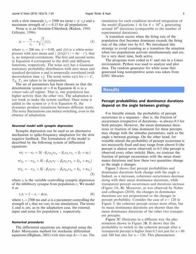
with a slow timescale sa¼ 2500 ms (note s� sa) and amaximum strength of c ¼ 0.15 for all populations.

Noise ni is an Ornstein-Uhlenbeck (Risken, 1989;Gillespie, 1996):

ni ¼ �nissþ r

ffiffiffiffi2

ss

rnðtÞ; ð4Þ

where ss ¼ 200 ms, r ¼ 0.08, and n(t) is a white-noiseprocess with zero mean and h n(t)n(t0) i ¼ d(t – t0), thatis, no temporal correlations. The first and second termsin Equation 4 correspond to the drift and diffusionfunctions, respectively. The noise ni(t) has a Gaussianstationary probability distribution with zero mean andstandard deviation r and is temporally correlated (withdecorrelation time ss). The noise terms ni(t) for i ¼ C,TR, TL are taken to be independent.

The set of parameters has been chosen so that thedeterministic system (r¼ 0 in Equation 4) is in awinner-take-all regime. That is, one population hashigher activity than the other two. The adaptation istoo weak to make the system oscillate. Once noise isadded to the system (r 6¼ 0 in Equation 4), thedynamics produce transitions between different states.The noisy fluctuations can induce switching, even in theabsence of adaptation.

Neuronal model with synaptic depression

Synaptic depression can be used as an alternativemechanism to spike-frequency adaptation for the slownegative feedback. The formulation of the model isdescribed by the following system of differentialequations:

srC ¼ �rC þ Sð�b1sTRrTR� b1sTL

rTLþ IC þ nCÞ

srTR¼ �rTR

þ Sð�b1sCrC � b2sTLrTLþ ITR

þ nTRÞ

srTL¼ �rTL

þ Sð�b1sCrC � b2sTRrTRþ ITL

þ nTLÞð5Þ

where si is the variable controlling synaptic depressionof the inhibitory synapse from population ri. We modelit as

sssi ¼ 1� si � /siri ð6Þwhere ss¼ 2500 ms and u is a parameter controlling thestrength of si that we vary in our simulations. The termsIi and ni are, as in the adaptation case, the externalinput and noise for population i, respectively.

Numerical procedures

The differential equations are integrated using theEuler–Maruyama method for stochastic differentialequations (Higham, 2001) with time step Dt¼1 ms. The

simulation for each condition involved integration ofthe model (Equations 1–4) for 4 · 104 s, generatingaround 104 durations (comparable to the number ofexperimental durations).

A transition occurs when the firing rate of thepopulation that becomes dominant exceeds the firingrate of the other two by 0.5. We introduced thisstrategy to avoid counting as a transition the situationwhen two populations activate simultaneously and are,for a very short time, both active.

The programs were coded in C and run in a Linuxenvironment. Python was used to analyze and plotdata. The random generator for white noise thatgenerated long nonrepetitive series was taken fromGNU libraries.

Results

Percept probabilities and dominance durationsdepend on the angle between gratings

For bistable stimuli, the probability of perceptoccurrence in a sequence—that is, the fraction ofoccurrences irrespective of durations—is always 0.5 forboth percepts. However, the mean dominance dura-tions or fraction of time dominant for these perceptsmay change with the stimulus parameters, such as theangle a between gratings. On the other hand, fortristable stimuli the probability of percept occurrence isnot necessarily fixed and may range from almost 0 (thepercept is almost never observed) to 0.5 (the percept isobserved every other switch). Here, we contrast thefraction of percept occurrences with the mean domi-nance durations and how these two quantities changeas the angle a changes.

Figure 3 shows that percept probabilities anddominance durations both change with the angle a.Indeed, as a increases, coherence occurrences decreasealong with their mean dominance durations, whiletransparent percept occurrences and durations increase(Figure 3A, B). Moreover, as was observed by Naberand colleagues (2010), the changes in dominancedurations are not proportional to the changes inpercept probability. Consider the case of a ¼ 120 inFigure 3; the coherent percept occurs more often, butits mean dominance durations are shorter than themean dominance durations of the other two transpar-ent percepts.

Figure 3C illustrates in a different way the phe-nomenon shown in Figure 3B: It shows that theprobability to switch to the coherent percept after atransparent percept is higher than 0.5 not just for a¼80and 100 but also for a¼ 120. This phenomenon

Journal of Vision (2014) 14(3):19, 1–24 Huguet, Rinzel, & Hupe 6

indicates an asymmetry in the system, showing a cleartendency to visit the coherent percept more often.

Model reproduces experimental data

Using the model described earlier, we identifiedinhibition and input strength as playing essential rolesin determining the mean dominance durations andpercept probabilities. As the angle a increases, weincrease the input strength to the transparent percepts(ITL

and ITR) and reduce the input strength to the

coherent percept (IC). These changes in the inputstrength increase both the mean dominance durationsand percept probabilities of the transparent percepts,while decreasing those of the coherent one. As a result,the percept with longer dominance durations alsoshows a higher probability of occurring.

In order to account for the effect observed for a¼120, where the mean dominance durations for coher-ence are shorter than those for transparent percepts,while coherence occurs more often, we propose

unbalanced inhibition: The two transparent popula-tions inhibit each other more strongly than they inhibitthe coherent one (b2 . b1 in Equation 1; see also Figure2), making the latter more dominant and more likely tooccur. We refer the reader to the ‘‘Dynamics of themodel’’ subsection later and Unbalanced inhibition andinput strength in Appendix 1 for more details. Oursimulated results agree with those obtained in experi-ments (see Figure 3; compare top with bottom plots).

Histograms of dominance durations are wellapproximated by log-normal or gammadistributions

In bistable rivalry, the histograms of dominancedurations are unimodal and skewed, with a long tail atlong durations. Typically, they are well approximatedby log-normal or gamma distributions (Levelt, 1968;Lehky, 1995; Hupe & Rubin, 2003). We exploredwhether dominance durations for tristable visual plaids

Figure 3. Statistics of switching: dependence on parameter a for psychophysics experiments (top) and for model simulations (bottom).

(A) Mean of the natural logarithm of the dominance durations expressed in milliseconds (seconds in parentheses; for the

experimental data, N¼6,516 durations, some epochs were removed, see Methods). (B) Percept probabilities in each trial (proportion

of number of occurrences (for the experimental data, N¼ 6,817 percepts). (C) Probability to switch to the coherent percept after a

transparent percept (for the experimental data, N¼ 3,752 sequences). Bars represent the means, and error bars are plus and minus

one standard error estimated by ANOVA models including the variable subject as a random factor (here and in all the subsequent

figures). Parameter values for the model are given in Methods. We used the same parameter values throughout the article, unless

stated otherwise.

Journal of Vision (2014) 14(3):19, 1–24 Huguet, Rinzel, & Hupe 7

had the same distributions as the ones observed forbistable stimuli. Moreover, since visual plaids can bealso interpreted as bistable when the observer is askedto report only whether the plaid was perceived ascoherent or transparent (without taking into accountthe depth reversals—see Figure 1), we also looked atthe distributions of dominance durations for aggre-gated transparent percepts.

Figure 4 shows the distributions of the normalizeddominance durations (NDDs) for the coherent percept(A), for aggregated consecutive transparent percepts(B), and for depth-segregated transparent percepts (C).To compute the normalized dominance durations, wedivided the durations by the median duration of eachpercept type for each subject (experiments) and a value(experiments and model). Histograms for the modelwere normalized to have an area of 1.

Histograms of dominance durations can be approx-imated by a log-normal or gamma distribution, as inthe bistable case. Following Moreno-Bote and col-leagues (2007), these distributions suggest that the noisein the system is ultimately responsible for switching. Inthat study, it was shown that when switching is

dominated by adaptation, histograms have a normaldistribution, but when adaptation is weakened, effec-tively giving more weight to noise, the histogramgradually evolves into a skewed one (log-normal/gamma).

Thus, in order to reproduce the experimental results,we have chosen a set of parameters for which thedeterministic system (Equation 1) with ni ¼ 0 (noiseterm) operates in a winner-take-all regime. Indeed, thesystem has three stable fixed points. Without noise, thetrajectories remain in one of these three attractors (eachone corresponding to a different percept) and noswitching occurs. When noise is restored, the trajecto-ries start to switch between these three states. See‘‘Dynamics of the model’’ and Balance betweenadaptation, noise, and input strength in Appendix 1 formore details.

Figure 4 shows the best fits by a log-normaldistribution (red) and by a gamma distribution (green).The quality of these fits is very similar. Notice that themodel can reproduce the histograms in both cases,when the stimulus is treated as bistable and when it istreated as tristable.

Figure 4. Histograms of dominance durations are well-approximated by log-normal or gamma distributions. Distributions of the

Normalized Dominance Durations (NDD; see text) for experiments (top) and simulations (bottom) pooled across the three values of

the angle (808, 1008, 1208) for (A) coherent percepts; (B) transparent aggregated percepts, obtained by aggregating consecutive TL

and TR percepts into a single percept; and (C) transparent percepts TL and TR. The red line is the best fit to log-normal distribution

fln(x)¼ 1/(xrffiffiffiffiffiffi2pp

)exp(�(ln(x) – l)2/(2r2)) and the green line is the best fit to gamma distribution fC(x)¼1/C(a)kaxa�1exp(�kx). For the

model, best fit to gamma distribution has a¼ 2.53, k¼ 2.22 (A); a¼ 3.9, k¼ 3.6 (B); and a¼ 3.65, k¼ 3.35 (C); best fit to log-normal

distribution has r¼ 0.66, l ¼�0.03 (A); r ¼ 0.52, l ¼�0.01 (B); and r ¼ 0.54, l ¼�0.02 (C).

Journal of Vision (2014) 14(3):19, 1–24 Huguet, Rinzel, & Hupe 8

Coherent percept duration affects the

probability of a switch back and provides

evidence for adaptation

As opposed to bistable percepts, where the onlypossibility is alternation between the two percepts, in thetristable case we can look at the probability of the next

percept’s being a switch back—the same percept as theprevious one—or a switch forward—a different perceptfrom the previous one (we adopt the terminology fromNaber et al., 2010). Moreover, we can ask whether thisprobability depends on the dominance durations (Figure5A).

For symmetry reasons, we focus here on tripletsconsisting of two transparent percepts interleaved with

Figure 5. The probability that two transparent percepts when interleaved with a coherent percept have the same depth pattern

increases as the duration of the coherent percept lengthens and decreases as the duration of the preceding transparent percept

lengthens. (A) Given a triplet of the form T1 CT2 in the perceptual sequence for a¼100 (T1 and T2 stand for both TL and TR), we show

the probability of a switch back, that is T1¼ T2, as a function of the duration of the coherent percept (B) and the first transparent

percept (C). Triplets are ordered according to the dominance durations of the intermediate coherent percept (B) or the first

transparent percept (C) in the triplet and then grouped in 10 bins of equal size (for experiments, n¼ 100, except for the last bin, n¼107). The coordinates of each dot are the middle point of each bin and the proportion of triplets in that bin that are a switch back.

Notice that the probability of a switch back is on average below the chance level of 0.5. The red line is the linear regression and the

blue line is the sigmoid fit; r is the correlation coefficient, and p-values are below or about 0.01 for both experiments and model. Fits

for experimental data were obtained by excluding the first data point (see text).

Journal of Vision (2014) 14(3):19, 1–24 Huguet, Rinzel, & Hupe 9

a coherent one. We denote them by T1 CT2, where T1

and T2 stand for both TL and TR. Indeed, we observedthat percept probabilities as well as mean dominancedurations for TL and TR are the same (see Figure 3A,B). So the next-percept probability when the currentpercept is coherent is 0.5 for both TL and TR. Hence,when we look at the next-percept probability as afunction of the previous percept—when the currentpercept is coherent—we know that any change in theprobability is due to perceptual history dependence andnot any other intrinsic asymmetry in the mechanism.Notice that this is not case when the current percept istransparent, because results show (see Figure 3C) thatit is more likely to switch to a coherent percept than toa transparent one. So there is already an intrinsic biastowards coherence, meaning that when the currentpercept is transparent and the previous one has beencoherent, the probability of switching back is biased bythis intrinsic predominance.

Figure 5B shows the probability that the twotransparent percepts in the triplet T1 CT2, Ti � {TL,TR}, have the same depth pattern (i.e., T1¼ T2)—whatwe call a switch back—as a function of the duration ofthe intermediate coherent percept C. It clearly showsthat the probability of a switch back increases as theduration of the coherent percept increases, andsaturates at 0.5 (chance level).

Notice, however, that the experimental data showthat for very short coherent durations, the probabilityto switch back is well above zero (open circle in Figure5B). We excluded this point (considered as an outlier)to fit the functions. Without excluding it, fits were ofcourse not as good, but the increase of switches back asa function of coherent duration was always highlysignificant (and present in every subject). So includingthis point in the data analysis or not would not changethe main conclusions of this study.

Further exploration of the effect of short coherentdurations on switch-back probabilities would berequired, but it might prove difficult because theseevents are rare for conditions of equiprobabilitybetween percepts. In addition, short percepts may notbe reported accurately. Indeed, the data for the first bincorrespond to coherent durations that are between 200ms and 1 s. They may therefore include some errors inthe button presses. But on the other hand, somesubjects may not report percepts that are too short.Individual data were quite variable indeed (as expected,given the limited power for such analysis), with twosubjects having a clear higher switch-back proportionfor very short durations and three subjects clearly notshowing that phenomenon. We should keep in mindthat this high probability of switch back for shortdurations may correspond to a real mechanism notincluded in the model if, for example, it corresponds tosome priming effect, like the tendency to report the

same percept for brief interruptions of the stimulus(Leopold, Wilke, Maier, & Logothetis, 2002; Maier,Wilke, Logothetis, & Leopold, 2003). The possibleaddition of this mechanism should not, however, affectthe mechanisms that we reveal here.

We also explored whether the durations of the firsttransparent percept in the triplet influence switchingprobabilities. Figure 5C shows the probability ofswitching back as a function of the mean dominancedurations for the first transparent perceptT1 in the tripletT1 CT2. Although the dependence is less strong than forthe coherent durations, results show that the probabilityof a switch back is higher if T1 is short.

We chose a¼ 100 for Figure 5B and C in order toexplore the relationship between coherent duration andprobability of switching back with everything else beingequal (i.e., independent of any other features in theresponse properties). Moreover, we found the largestvariability of coherent durations for a ¼ 100. Weobserved similar trends for a¼ 80 and a¼ 120 (resultsnot shown). Further, a similar and even strongerrelationship between coherent-percept duration andswitch-back probability was observed in two otherindependent data sets collected over many subjects andpooled across different plaid parameters (Hupe, 2010;these data were presented in Hupe & Pressnitzer, 2012;see also Appendix 2).

We interpret this result as showing evidence for anegative feedback mechanism that acts at a slowertimescale than the firing-rate variable r. We found that asubtractive negative feedback opposing the excitatoryinput, typically referred as spike-frequency adaptationand represented by the variable a in Equation 1, isessential to explain the mentioned effect. Thus, in ourmodel (Equation 1), when a percept becomes dominant,it starts to recruit some adaptation. The adaptationrecruited will prevent this percept from becomingdominant again immediately after being suppressed,making it very unlikely for this percept to recur after ashort duration. Moreover, the less time a percept hasbeen active, the less adaptation this percept has recruitedwhile active and the more likely a reappearance of thispercept. In ‘‘Dynamics of the model’’ we discuss thismechanism in more detail. The simulations agree withthe experimental results (Figure 5).

Other possible mechanisms for negative feedbackinclude synaptic depression—a divisive mechanismacting directly on the inhibitory input; the depressionvariable multiplies the term that models inhibitionstrength during prolonged firing (see Equations 5 and6). When we implemented synaptic depression in ourmodel, we were unable to reproduce the probabilitydependence on durations. We refer the reader toDifferent roles for spike-frequency adaptation andsynaptic depression in Appendix 1 for a more detailed

Journal of Vision (2014) 14(3):19, 1–24 Huguet, Rinzel, & Hupe 10

mathematical discussion on the two negative feedbackmechanisms.

Noise-driven switching removes correlations indominance durations

Results in Figure 5 suggest that T1 durations arenegatively correlated with C durations: Switch-backtriplets (T1¼ T2) are more likely for short T1 and longC, while switch-forward triplets (T1 6¼ T2) are morelikely for long T1 and short C. Figure 6A shows Cdurations plotted against T1 durations for T1 CT2

triplets. T1 and C percept durations were normalized,independently, by their median durations for eachsubject. We included T1 and C of T1 CT2 sequencesonly for a¼ 100, in order to allow the comparison withthe analysis of percept choice in Figure 5. The lack ofany strong correlation is clearly seen, in agreement withprevious observations (see Rubin and Hupe, 2005, forexample). We interpret this lack as evidence that boththe duration of T1 and the duration of C contribute tothe probability of a switch back, even though bothdurations are not correlated with each other. In themodel, such an absence of relationship is captured byhaving a high level of noise (noise-driven attractormodel; see Figure 6B). Thus, when considering perceptduration independently of percept choice, there is noevidence of adaptation.

Dynamics of the model

In the previous sections, we have described severalfeatures of the system (dominance durations, percept

probabilities, distributions, and switch-back probabili-ties) and discussed how the external input, inhibition,adaptation, and noise affect them. We offer here amechanistic explanation via a simple schematic for thedynamics of switching in the model that combines theseelements (Figure 7A). A population becomes activewhen the total input (Figure 7Ba) to the input–outputfunction S given in Equation 2 (Figure 7A, inset) isabove the threshold h. The model parameters are chosenso that when a population becomes active, it suppressesthe other two, ensuring that only one population isactive at the same time. The total input of the activepopulation (Figure 7Ba, time t1) decreases over time dueto the adaptation current (Figure 7Bc, time t1), while thesuppressed populations recover from adaptation, bring-ing their total input closer to the threshold h. Sinceadaptation and input strength have been chosen so thatthe total input never crosses the threshold, the systemwould never show alternations without the presence ofnoise. Indeed, the noise-driven fluctuations may bringthe total input of the suppressed populations abovethreshold, causing the switching.

Notice that in this regime of parameters, the totalinput for the suppressed percepts is closer to thethreshold than is the input for the active population,suggesting that the transitions occur due to an escapemechanism (the total input to one of the suppressedpopulations crosses threshold, causing the suppressionof the active one). We could have also considered thecase where the active population is closer to thethreshold and the transition occurs due to a releasemechanism (the total input to the active populationfalls below the threshold, allowing the suppressedpopulations to take over; see Shpiro, Curtu, Rinzel, &Rubin, 2007). In our simulations, an escape mecha-nism introduces more variability to the dominance

Figure 6. Durations of T1 and C for T1 CT2 sequences for experiments (A) and model (B). For experimental data, plot durations were

normalized, independently, by the median durations for each subject. Correlations are absent or small. Here, N is the number of dots,

R2 is the coefficient of determination, and p is the p-value.

Journal of Vision (2014) 14(3):19, 1–24 Huguet, Rinzel, & Hupe 11

durations, which fits better with experimental obser-vations (see Balance between adaptation, noise, andinput strength in Appendix 1) than a release mecha-nism, but we did not observe any other remarkabledifferences that are relevant for visual plaids (resultsnot shown).

Just after coherence is suppressed, its total input isbelow the total input for the other suppressedtransparent population (Figure 7Ba, time t2). However,if the active population TR remains active for longenough (based on the timescale of adaptation),coherence recovers from adaptation and its total inputapproaches threshold. Moreover, since coherencereceives less inhibition than the other suppressedtransparent population TL from the active TR (unbal-anced inhibition), its total input overtakes that of theother suppressed percept, making it more likely thatcoherence will reappear.

Thus, for equal inputs to the three populations,coherence will be more likely to appear, while itsdurations will be shorter compared to the ones for theother transparent percepts. Indeed, when a populationbecomes active, it can be overtaken by two populations.If one of these two suppressed populations is pushedfurther down from the threshold, the chances of its beingovertaken are reduced and the dominance durations ofthe active population lengthen. That is the case whentransparent populations are active (see Unbalancedinhibition and input strength in Appendix 1).

We next examine Figure 7 to gain a furtherunderstanding of the dependence of switch-backprobabilities on adaptation strength. Indeed, when thecoherent population is active, the two suppressedtransparent populations have different total inputsbecause of adaptation (see Figure 7Ba, times t1 and t3).The suppressed population that was active before thecurrent state still has some adaptation, and therefore itstotal input is lower and further from the threshold thanthe total input of the other suppressed population.Hence, if coherent dominance durations are short, aswitch forward is more likely than a switch back. Ascoherent durations become longer, the total input ofboth suppressed populations becomes similar and theprobability of a depth switch becomes 0.5 (see Figure7Ba, times t1 and t3). Moreover, if the first transparentpopulation in the triplet was active for a long time, itrecruited more adaptation and will have less probabil-ity of reappearing for a longer time.

The question that arises now is what the balance isbetween input, inhibition, adaptation, and noise thatgenerates the desired output. Of course, a system that isdominated by adaptation would show small variability,while a system dominated by noise would showswitching probabilities independent of percept dura-tions and exponential distributions for dominancedurations (peaked around the timescale of noise orderof 200 ms). Moreover, the relative inputs to thepopulations will contribute to the dominance durationsand percept probabilities. We include a mathematicalexploration of this balance in Appendix 1, underBalance between adaptation, noise, and input strengthand Unbalanced inhibition and input strength.

Figure 7. Dynamical properties of the model. (A) Schematic

representation of the mechanism underlying transitions be-

tween suppressed and dominant states. The height of the bars

indicates the total input to the input–output function for each

population at three different times indicated in (B). (B) Time

courses of the total input minus the noise term ni (Ba), activity

(Bb), and adaptation (Bc) of the three populations: coherent

(red), transparent right (green), and transparent left (blue). The

horizontal line in (A) and (Ba) corresponds to the threshold (¼0.2) of the input–output function [inset, (A)]. When the bar is

above the threshold, the population is active (activity near 1),

and when it is below the threshold, the population is

suppressed (activity near 0)—see the corresponding times in

(Ba) and (Bb). The arrow indicates the effect of adaptation on

the total input. A downward arrow indicates that adaptation is

increasing for the active population, reducing the total input for

that population [see the corresponding times in (Ba) and (Bc)].

An upward arrow indicates that adaptation is decreasing for the

suppressed population, increasing the total input for that

population [see the corresponding times in (Ba) and (Bc)].

Notice that adaptation drives the input level closer to the

transition threshold but still well above or below it.

Journal of Vision (2014) 14(3):19, 1–24 Huguet, Rinzel, & Hupe 12

Noise and adaptation

A unique contribution from tristability is that ithelps to constrain more precisely the balance betweennoise and adaptation beyond the constraints forbistability. Hitherto, the discussion about the role ofnoise and adaptation in the switching mechanism forbistable models has mainly focused on how they affectthe histograms for dominance durations and the lack ofcorrelations for successive percepts. For tristability, wecan add another constraint: the bias in switch-backprobabilities. If adaptation is removed from the systemor noise is too strong, the switch-back probability inFigure 5 remains constant at 0.5 independent of thedurations of coherence. See also Balance betweenadaptation, noise, and input strength in Appendix 1.

Using the parameters of the model that best fit thedata, we removed adaptation from the model andfound that distributions were exponential instead oflog-normal or gamma; there was no dependence of theswitch-back probability on the coherence duration, anddurations increased (switch rate decreased). For in-stance, for a ¼ 120, we found that the mean perceptdurations doubled (a halving of the switch rate).Namely, within a 3-min run, we had on average 39switches with adaptation (for experiments, we had arange from 19 to 45); without adaptation we wouldhave had 21 switches. For a ¼ 80, we observed areduction of switches from 30 to 10 in 3 min. Theseobservations relate to the results of Blake, Sobel, andGilroy (2003), who managed to reduce the amount ofadaptation in the system by means of a visual stimulusthat was moving in the visual field so that it wasconstantly engaging unadapted neural tissue. They

found, as our numerical model predicts, that perceptualalternations were slowed down when adaptation wasreduced.

Other possible network architectures

So far, we have considered a model architecture inwhich three populations compete at the same levelthrough direct cross-inhibition (Figure 2). We alsoconsidered a hierarchical architecture for the model(Figure 8A), in which depth and movement areencoded by two different groups of populations(motion segregation activates depth perception). Themodel consists of four populations: The first pair ofpopulations, labeled C and T, encode motion percep-tion (coherence vs. transparency). They competethrough inhibition. When the population encodingtransparency is active (coherence is suppressed), asecond pair of populations (excited by population T)is recruited. Those two subpopulations, labeled TR

and TL, encode depth perception (which driftinggrating is on top), and they compete throughinhibition as well.

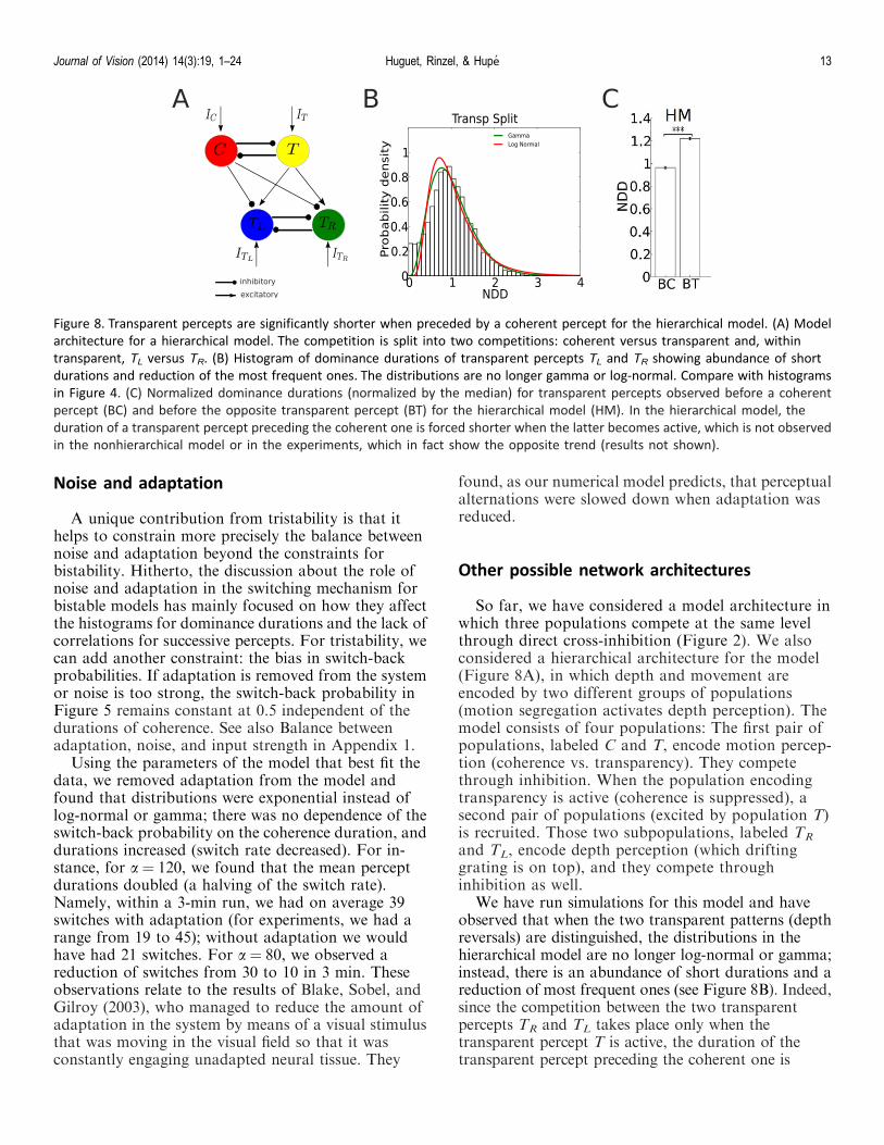
We have run simulations for this model and haveobserved that when the two transparent patterns (depthreversals) are distinguished, the distributions in thehierarchical model are no longer log-normal or gamma;instead, there is an abundance of short durations and areduction of most frequent ones (see Figure 8B). Indeed,since the competition between the two transparentpercepts TR and TL takes place only when thetransparent percept T is active, the duration of thetransparent percept preceding the coherent one is

Figure 8. Transparent percepts are significantly shorter when preceded by a coherent percept for the hierarchical model. (A) Model

architecture for a hierarchical model. The competition is split into two competitions: coherent versus transparent and, within

transparent, TL versus TR. (B) Histogram of dominance durations of transparent percepts TL and TR showing abundance of short

durations and reduction of the most frequent ones. The distributions are no longer gamma or log-normal. Compare with histograms

in Figure 4. (C) Normalized dominance durations (normalized by the median) for transparent percepts observed before a coherent

percept (BC) and before the opposite transparent percept (BT) for the hierarchical model (HM). In the hierarchical model, the

duration of a transparent percept preceding the coherent one is forced shorter when the latter becomes active, which is not observed

in the nonhierarchical model or in the experiments, which in fact show the opposite trend (results not shown).

Journal of Vision (2014) 14(3):19, 1–24 Huguet, Rinzel, & Hupe 13

prematurely terminated when coherence becomes active.Hence, the mean dominance durations of the transpar-ent percepts preceding a coherent one are significantlyshorter than those of the transparent percepts precedingthe opposite transparent percept (see Figure 8C).

Based on firing-rate models, our results suggest thata nonhierarchical architecture where motion is encodedtogether with depth can better fit the experimentalresults. We do not claim that the architecture describedin Figure 2 is the only or optimal possibility. Indeed, wethink that several network architectures (probablymore complex) could produce similar results. However,we emphasize that the one considered herein (Figure 2)is the simplest architecture that could encode a directinfluence between the individual transparent perceptsand the coherent one.

Discussion

We have studied the dynamics of perceptual switchingfor tristable visual plaids.We have developed an idealizedneuronal competition model (that extends the existingmodels for bistability) that can account for the results,reported here, from behavioral experiments of switching.Working with this relatively simple model (with minimaldegrees of freedom), we have discovered that noise andadaptation have different roles. Thus, while noise isultimately responsible for switches (adaptation alonecannot trigger a switch) and thereby controls perceptdurations, adaptation affects the percept choice.

Different roles for noise and adaptation

The issue of perceptual history dependence and, inconsequence, the roles that adaptation and noise playin switching, has been central in discussions onbinocular rivalry. Several researchers have reported theabsence of correlations between successive dominancedurations (Fox & Hermann, 1967; Levelt, 1968; Lehky,1995; Logothetis et al., 1996; Rubin & Hupe, 2005),suggesting that perceptual multistability is a memory-less process; perceptual history does not affect thedurations of subsequent percepts. This observation hasbeen interpreted as meaning that adaptation plays asecondary role in the switching mechanism and thatswitching is dominated by noise (Brascamp et al., 2006;Lankheet, 2006; Moreno-Bote et al., 2007).

However, other studies exploring interrupted bistablestimuli have suggested the possibility of priming (implicitmemory effect) in bistable rivalry. When the presenta-tion of an ambiguous stimulus is interrupted by blankpresentations or other visual stimuli, subjects tend toreport restarting with the just-previous percept (Leopold

et al., 2002; Maier et al., 2003). This ‘‘stabilizationeffect’’ depends not only on the latest percept before theinterruption but also on the previous perceptual historythat traces back several seconds (Brascamp et al., 2008;Pastukhov & Braun, 2008). Although percept choice andpercept switching may involve different processes(Noest, van Ee, Nijs, & van Wezel, 2007), these resultssuggest that a form of adaptation must be present inambiguous visual perception. Moreover, recent resultsfor other types of tristable visual stimuli also point infavor of an adaptation model to account for certainaspects of transitions and durations (Naber et al., 2010;Wallis & Ringelhan, 2013).

Our results for tristable percepts indicate that bothnoise and adaptation are present in the system but theyhave different roles, thus shedding new light on alongstanding controversy. In the model, we have chosenparameters so that the balance between noise andadaptation causes noise to drive the switches—adapta-tion is too weak to produce switches by itself—andcauses adaptation to determine the percept switch—adaptation, even if weak, is strong enough to bias theswitch-back probabilities. Indeed, short durations of thecurrent percept increase the probability of a switchforward; from the two suppressed percepts, the lessadapted is, on average, favored to become active (seeFigure 7A). On the contrary, long durations reduce anyadvantages to the suppressed percepts, making themequally likely to become active; therefore, the ‘‘memory’’of the last transparent percept is erased (see Figure 5).Moreover, adaptation decays or builds up on a timescaleof the order of a few seconds, so one might expect thatits effect would be erased after one percept. Thus, theadaptation process has the effect of creating a sort ofmemory as well as disfavoring early transitions (Mor-eno-Bote et al., 2007).

The nature of the slow adaptation process has astrong influence in this perceptual bias. In our simplemodel, we could explain the trends shown in Figure 5only with spike-frequency adaptation (subtractivenegative feedback), not with synaptic depression(divisive negative feedback), suggesting a differentfunctional role for these slow negative feedbackprocesses (see Different roles for spike-frequencyadaptation and synaptic depression in Appendix 1).Previous studies analyzing different types of slowadaptation, divisive versus subtractive, have notreported functional differences between these twomechanisms in bistable rivalry (Shpiro et al., 2007;Shpiro et al., 2009).

Parametric manipulations

The discovery of different roles for noise andadaptation was made by studying a very specific set of

Journal of Vision (2014) 14(3):19, 1–24 Huguet, Rinzel, & Hupe 14

stimuli and parameters. This was necessary to identifythe mechanisms with constant input. Such a strongconstraint could question the generalization of ourresult: Would similar results be obtained for differentparameters and stimuli?

For parameters of visual plaids, extensive studiesof the long-term dynamics of plaids (Hupe & Rubin,2003, 2004; Rubin & Hupe, 2005; Pressnitzer &Hupe, 2006; Hupe, Joffo, & Pressnitzer, 2008; Hupe& Pressnitzer, 2012) have shown that the effects ofparametric manipulations studied so far are inde-pendent of each other. In particular, this is the casefor motion direction (Hupe & Rubin, 2004) andspeed (Hupe & Rubin, 2003), both parametersproducing effects notably independent of a. Onecould, however, question whether the main unex-pected empirical observations could have been due tothe choice of always having the coherent motionaligned with the vertical direction. Indeed, thisvertical symmetry of the stimulus may have led to thecoherent percept (also vertical) being more oftenvisited than the two transparent percepts (alsooblique), as shown in Figure 3. Even though thecritical relationship between the duration of thecoherent percept and the switch-back probability(Figure 5B) may be more difficult to explain by thevertical symmetry of the stimulus, one may alsolegitimately wonder whether such a result maygeneralize to other parametric conditions. Indepen-dent data were in fact collected earlier by J-MHconfirming both results over a larger range ofparameters. In Appendix 2 we include a summary ofthese experiments, for which different directions wereused. For that reason as well as wanting as muchempirical data as possible for a single condition, wedecided to limit the set of parameters to be explored.Indeed, the present data are stronger because theywere obtained on a larger data set without para-metric manipulation (10 repetitions of 3-min trials,that is 15 times as many sequences for each stimulusand subject as in the previous data set).

For other tristable stimuli, several observationsmade by Naber and colleagues (2010) and Wallis andRingelhan (2013) after pooling data over severalparameters showed some commonalities with ourbehavioral data and could be accounted for by ourmodel with the aforementioned roles for noise andadaptation. For instance, Naber and colleagues (2010)reported that switch-back triplets typically have longerdurations than average for the intermediate percept (inour case, C) and shorter durations than average for thefirst percept in the triplet (in our case, T1). On the otherhand, Wallis and Ringelhan (2013) reported that theswitch-back transitions were longer than the switch-forward ones, a property that was also observed in ourmodel (results not shown). Although we may need to

adjust several parameters in the model to reproduce thedominance durations and percept probabilities of eachparticular stimulus, the roles of noise and adaptation inthe model described herein will remain unchanged. Thefact that histograms of dominance durations in ourmodel match across a multitude of stimuli (Naber et al.,2010; Wallis & Ringelhan, 2013, supplementary mate-rial) provides grounds for this speculation.

Actually, when we considered a different architec-ture for the model, such as the hierarchical one inFigure 8, the roles of noise and adaptation were thesame as for the same-level architecture. Of course, theexact parameters of the model depend on the specificarchitecture of the model, but the roles they play in thedynamics do not. Indeed, the hierarchical model thatcould best fit the experimental data was noise drivenbut could reproduce the switch-back dependence onpercept duration with adaptation (results not shown).

The role of inhibition and input strength inpercept duration and percept choice

Biases that may be specific to this paradigm shouldnot be confounded with general mechanisms. Here, thehigher number of occurrences of the coherent percept(see Figure 3) could simply be accounted for byunbalanced inhibition. Previous work on bistablemodels has shown that dominance durations areaffected by the input strength (Laing & Chow, 2002;Shpiro et al., 2007), but in bistable stimuli, perceptprobabilities are always fixed at 0.5. Here, we haveshown that inhibition and input strength affect both thedominance durations and percept probabilities and therelation between them (see ‘‘Model fits with theexperimental data,’’ earlier). Moreover, we have shownhow inhibition and input strength can be manipulatedasymmetrically to adjust dominance durations andpercept probabilities independently (see also Unbal-anced inhibition and input strength in Appendix 1).From this understanding, one can then adjust themodel to other experimental data. For instance, if astimulus leads to dominance durations and perceptprobabilities that are equally dominant in both meanand percept probability (see, for example, Wallis andRingelhan, 2013) we suggest symmetric inhibition andinput strength.

Visual plaids and their relevance for motion anddepth perception

The same-level model was better than the hierarchi-cal model for fitting the experimental data. This hasinteresting consequences for the mechanisms of motionsegmentation and depth ordering (Adelson & Mov-

Journal of Vision (2014) 14(3):19, 1–24 Huguet, Rinzel, & Hupe 15

shon, 1982; Hupe & Rubin, 2003; Hupe & Pressnitzer,2012). The underlying ambiguity here comes from thephenomenon known as the aperture problem. Thedirection of movement of a bar with occluded edgescannot be determined. In the absence of other externalcues, the subject tends to perceive the velocity in thedirection normal to the stripes. When two gratings aresuperimposed, they can be perceived as movingindependently (each one in the direction orthogonal toits stripes) or coherently (both gratings in the samedirection). While transparency is perceived, sincegratings move in opposite directions and shareintersections, there is a conflict that is resolved byseparating the object into two and placing them ondifferent planes. Since the intersections can be assignedequally well to both gratings, alternation occurs.

A reasonable question is whether incoherent motionleads to depth perception or whether depth perceptionis encoded together with motion segregation. Thearchitecture of our model is designed so that these twocues influence each other with no hierarchy, so one isnot leading the other. Simulations of our model with ahierarchical architecture (motion and depth are en-coded separately) were not able to reproduce experi-mental results (Figure 8).

Existing physiological data from the middle tempo-ral visual area (MT) of the visual cortex provide aneural substrate for a nonhierarchical model architec-ture (see Born & Bradley, 2005, for an MT review).Neurons in the visual area MT are involved indetection of motion direction; they are selective to aparticular direction of motion (their activity is en-hanced or reduced depending on whether a preferred ornonpreferred motion occurs, respectively; Albright,Desimone, & Gross, 1984; Britten, Shadlen, Newsome,& Movshon, 1992). Subsequent studies have suggestedthat MT is involved in the perception of depth as well(Bradley, Chang, & Andersen, 1998; DeAngelis, Cum-ming, & Newsome, 1998; Dodd, Krug, Cumming, &Parker, 2001). The suppression of MT responses due tononpreferred motion is reduced when the nonpreferredand preferred motions occur in separate depth planes(Bradley, Qian, & Andersen, 1995). Hence, placingopposing movements in different planes prevents thecancellation of the motion signal.

Limitations of the model

We emphasize that we did not attempt to account forall properties of visual plaids. Instead, we tried to keepthe model as simple as possible to allow for mathe-matical analysis of the parameters and still reproducethe most prominent features observed in psychophysicsexperiments. We believe that some of the remaining

features can be explained by straightforward extensionsof our model.

For instance, no attempt was made to include amechanism to deal with first-percept inertia, a phe-nomenon observed in experiments with visual plaids(Hupe & Rubin, 2003; Hupe & Pressnitzer, 2012). Thisrefers to a tendency, observed at the stimulus onset, forthe first percept (which is almost always coherent: first-percept bias) to be longer than the subsequent coherentones (see Hupe and Pressnitzer, 2012, for a suggestionof an additional mechanism to account for first-perceptinertia and for a simple explanation of first-perceptbias).

Two other observations may require additionalmechanisms, if confirmed: one subject with shorttransparent durations and a reverse relationship forswitch back, and the high switch-back probability forvery short durations of the intermediate percept (Figure5B). Once these additional phenomena are fullydocumented and explained, the simple model presentedhere may require additional variables, such as anadditional negative feedback, either slower or of adifferent type (divisive).

Plausible neural bases for noise and adaptation

We think that the inclusion of various additionalmechanisms should not change the essential roles ofnoise and adaptation identified in this study (yet wecannot prove it). We can speculate what these rolesmean for the neural correlates of multistable percep-tion. Neural correlates of visual bistable perceptionhave been observed in low-level areas (with fMRI:Tong & Engel, 2001; Wilson, Blake, & Lee, 2001;Haynes, Deichmann, & Rees, 2005; Lee, Blake, &Heeger, 2005, 2007; Wunderlich, Schneider, & Kastner,2005), high-level visual areas (with monkey electro-physiology: Leopold & Logothetis, 1999; Williams,Elfar, Eskandar, Toth, & Assad, 2003), and innonvisual parietal and frontal areas (Sterzer &Kleinschmidt, 2007). Among these neural correlates,some may relate to the percept consciously experienced,while others may relate to the mechanism of switching.The distinct roles of adaptation and noise that we havediscovered may help in clarifying the apparentlyconflicting results regarding the brain areas involved inmultistable perception. Adaptation is more likely toconcern the neural populations that encode eachcompeting percept, and therefore should be observedwithin the visual cortex. The time course that weobserved, for both adaptation of the dominant perceptand recovery of the suppressed percept, could be usedas a precise signature of the neural correlates. Simplylooking for the neural correlates of the perceivedinterpretations is not decisive, since once an interpre-

Journal of Vision (2014) 14(3):19, 1–24 Huguet, Rinzel, & Hupe 16

tation is selected, it may be both transmitted to higherlevel areas and fed back to lower visual areas, forexample for attention mechanisms (Watanabe et al.,2011). Looking for the dynamics of the neuralcorrelates of both the suppressed and the dominantpercepts would provide much more stringent criteria.Our model revealed the critical role of noise indetermining the time of switch. Noise in the modelcould reflect many different mechanisms, includingblinks and non-stimulus-related eye movements (thatchange the visual input) as well as high-level attentionand intention mechanisms. Our proposed role for noiseis therefore fully compatible with the involvement ofparietal and frontal structures (Sterzer & Kleinschmidt,2007). However, depending on the content of suchnoise, prefrontal activity may not be systematicallynecessary to trigger a switch, if other sources of noiseare available.

In sum, we propose that adaptation and noise areboth involved in perceptual alternations, but withdifferent roles: Noise controls the time of the switch,while adaptation controls which percept is next. Basedon our results, we think it is worthwhile andinteresting to pursue this proposal in other contexts ofperceptual multistability (which include a moregeneral group of experiences), to probe whether thereis a kind of structured response of the brain toambiguous stimuli.

Keywords: perceptual tristability, rivalry, ambiguousstimuli, firing-rate model, visual plaids, noise, adaptation

Acknowledgments

The research for this study was supported, in part,by i-math Fellowship ‘‘Proyectos flechados,’’ SwartzFoundation, ‘‘Juan de la Cierva’’ fellowship, MCyT/FEDER grant MTM2012-31714, and CUR-DIUEgrant 2009SGR859 (GH); and Agence Nationale deRecherche ANR-08-BLAN-0167-01 (J-MH). GHwants to acknowledge the use of the UPC AppliedMath cluster system for research computing. GH andJR thank the Mathematical Biosciences Institute (MBI)at Ohio State University for hospitality and supportduring long-term visits when the final version of themanuscript was written; GH especially appreciatesreceiving an Early Career Award from the MBI.

Commercial relationships: none.Corresponding author: Gemma Huguet.Email: gemma.huguet@upc.edu.Address: Department of Applied Mathematics I,Universitat Politecnica de Catalunya, Barcelona,Spain.

References

Adelson, E. H., & Movshon, J. A. (1982). Phenomenalcoherence of moving visual patterns. Nature, 300,523–525.

Albright, T. D., Desimone, R., & Gross, C. G. (1984).Columnar organization of directionally selectivecells in visual area MT of the macaque. Journal ofNeurophysiology, 51, 16–31.

Blake, R., & Logothetis, N. K. (2002). Visualcompetition. Nature Reviews Neuroscience, 3, 13–21.

Blake, R., Sobel, K. V., & Gilroy, L. A. (2003). Visualmotion retards alternations between conflictingperceptual interpretations. Neuron, 39, 869–878.

Born, R. T., & Bradley, D. C. (2005). Structure andfunction of visual area MT. Annual Review ofNeuroscience, 28, 157–189.

Bradley, D. C., Chang, G. C., & Andersen, R. A.(1998). Encoding of three-dimensional structure-from-motion by primate area MT neurons. Nature,392, 714–717.

Bradley, D. C., Qian, N., & Andersen, R. A. (1995).Integration of motion and stereopsis in middletemporal cortical area of macaques. Nature, 373,609–611.

Brascamp, J. W., Knapen, T. H., Kanai, R., Noest, A.J., van Ee, R., & van den Berg, A. V. (2008). Multi-timescale perceptual history resolves visual ambi-guity. PLoS ONE, 3(1), e1497.

Brascamp, J. W., van Ee, R., Noest, A. J., Jacobs, R.H., & van den Berg, A. V. (2006). The time courseof binocular rivalry reveals a fundamental role ofnoise. Journal of Vision, 6(11):8, 1244–1256, http://www.journalofvision.org/content/6/11/8, doi:10.1167/6.11.8. [PubMed] [Article]

Britten, K. H., Shadlen, M. N., Newsome, W. T., &Movshon, J. A. (1992). The analysis of visualmotion: A comparison of neuronal and psycho-physical performance. Journal of Neuroscience, 12,4745–4765.

Burton, G. (2002). Successor states in a four-stateambiguous figure. Psychonomic Bulletin and Re-view, 9, 292–297.

DeAngelis, G. C., Cumming, B. G., & Newsome, W. T.(1998). Cortical area MT and the perception ofstereoscopic depth. Nature, 394, 677–680.

Dodd, J. V., Krug, K., Cumming, B. G., & Parker, A.J. (2001). Perceptually bistable three-dimensionalfigures evoke high choice probabilities in corticalarea MT. Journal of Neuroscience, 21, 4809–4821.

Journal of Vision (2014) 14(3):19, 1–24 Huguet, Rinzel, & Hupe 17

Fox, R., & Hermann, J. (1967). Stochastic properties ofbinocular rivalry alternations. Perception & Psy-chophysics, 2, 432–436.

Gillespie, D. T. (1996). Exact numerical simulation ofthe Ornstein-Uhlenbeck process and its integral.Physical Review E, 54, 2084–2091.

Haynes, J. D., Deichmann, R., & Rees, G. (2005). Eye-specific effects of binocular rivalry in the humanlateral geniculate nucleus. Nature, 438, 496–499.

Hedges, J. H., Stocker, A. A., & Simoncelli, E. P.(2011). Optimal inference explains the perceptualcoherence of visual motion stimuli. Journal ofVision, 11(6):14, 1–16 , http://www.journalofvision.org/content/11/6/14, doi:10.1167/11.6.14.[PubMed] [Article]

Higham, D. J. (2001). An algorithmic introduction tonumerical simulation of stochastic differentialequations. SIAM Review, 43(3), 525–546, doi:10.1137/S0036144500378302.

Hupe, J. M., Joffo, L. M., & Pressnitzer, D. (2008).Bistability for audiovisual stimuli: Perceptual deci-sion is modality specific. Journal of Vision, 8(7):1,1–15, http://www.journalofvision.org/content/8/7/1, doi:10.1167/8.7.1. [PubMed] [Article]

Hupe, J. M., & Pressnitzer, D. (2012). The initial phaseof auditory and visual scene analysis. PhilosophicalTransactions of the Royal Society B: BiologicalSciences, 367, 942–953.

Hupe, J. M., & Rubin, N. (2003). The dynamics of bi-stable alternation in ambiguous motion displays: Afresh look at plaids. Vision Research, 43, 531–548.

Hupe, J. M., & Rubin, N. (2004). The oblique plaideffect. Vision Research, 44, 489–500.

Lago-Fernandez, L. F., & Deco, G. (2002). A model ofbinocular rivalry based on competition in IT.Neurocomputing, 44, 503–507.

Laing, C. R., & Chow, C. C. (2002). A spiking neuronmodel for binocular rivalry. Journal of Computa-tional Neuroscience, 12, 39–53.

Lankheet, M. J. (2006). Unraveling adaptation andmutual inhibition in perceptual rivalry. Journal ofVision, 6(4):1, 304–310, http://www.journalofvision.org/content/6/4/1, doi:10.1167/6.4.1. [PubMed][Article]

Lee, S. H., Blake, R., & Heeger, D. J. (2005). Travelingwaves of activity in primary visual cortex duringbinocular rivalry. Nature Neuroscience, 8, 22–23.

Lee, S. H., Blake, R., & Heeger, D. J. (2007). Hierarchyof cortical responses underlying binocular rivalry.Nature Neuroscience, 10, 1048–1054.

Lehky, S. R. (1995). Binocular rivalry is not chaotic.

Proceedings of the Royal Society B: BiologicalSciences, 259, 71–76.

Leopold, D. A., & Logothetis, N. K. (1999). Multi-stable phenomena: Changing views in perception.Trends in Cognitive Sciences (Regul. Ed.), 3, 254–264.

Leopold, D. A., Wilke, M., Maier, A., & Logothetis, N.K. (2002). Stable perception of visually ambiguouspatterns. Nature Neuroscience, 5, 605–609.

Levelt, W. J. M. (1968). On binocular rivalry. TheHague, Netherlands: Mouton.

Logothetis, N. K., Leopold, D. A., & Sheinberg, D. L.(1996). What is rivalling during binocular rivalry?Nature, 380, 621–624.

Long, G. M., & Toppino, T. C. (2004). Enduringinterest in perceptual ambiguity: Alternating viewsof reversible figures. Psychological Bulletin, 130,748–768.

Maier, A., Wilke, M., Logothetis, N. K., & Leopold,D. A. (2003). Perception of temporally interleavedambiguous patterns. Current Biology, 13, 1076–1085.

Moreno-Bote, R., Rinzel, J., & Rubin, N. (2007).Noise-induced alternations in an attractor networkmodel of perceptual bistability. Journal of Neuro-physiology, 98, 1125–1139.

Moreno-Bote, R., Shpiro, A., Rinzel, J., & Rubin, N.(2008). Bi-stable depth ordering of superimposedmoving gratings. Journal of Vision, 8(7):20, 1–13,http://www.journalofvision.org/content/8/7/20,doi:10.1167/8.7.20. [PubMed] [Article]

Naber, M., Gruenhage, G., & Einhauser, W. (2010).Tri-stable stimuli reveal interactions among subse-quent percepts: rivalry is biased by perceptualhistory. Vision Research, 50, 818–828.

Noest, A. J., van Ee, R., Nijs, M. M., & van Wezel, R.J. (2007). Percept-choice sequences driven byinterrupted ambiguous stimuli: A low-level neuralmodel. Journal of Vision, 7(8):10, 1–14, http://www.journalofvision.org/content/7/8/10, doi:10.1167/7.8.10. [PubMed] [Article]

Pastukhov, A., & Braun, J. (2008). A short-termmemory of multi-stable perception. Journal ofVision, 8(13):7, 1–14, http://www.journalofvision.org/content/8/13/7, doi:10.1167/8.13.7. [PubMed][Article]

Pastukhov, A., & Braun, J. (2011). Cumulative historyquantifies the role of neural adaptation in multi-stable perception. Journal of Vision, 11(10):12, 1–10, http://www.journalofvision.org/content/11/10/12, doi:10.1167/11.10.12. [PubMed] [Article]

Pastukhov, A., Garcia-Rodriguez, P. E., Haenicke, J.,

Journal of Vision (2014) 14(3):19, 1–24 Huguet, Rinzel, & Hupe 18

Guillamon, A., Deco, G., & Braun, J. (2013).Multi-stable perception balances stability andsensitivity. Frontiers in Computational Neurosci-ence, 7:17, 1–18.

Pressnitzer, D., & Hupe, J. M. (2006). Temporaldynamics of auditory and visual bistability revealcommon principles of perceptual organization.Current Biology, 16, 1351–1357.

Risken, H. (1989). The Fokker-Planck equation (2nded.). Berlin: Springer-Verlag, doi:10.1007/978-3-642-61544-3.

Rubin, N., & Hupe, J. M. (2005). Dynamics ofperceptual bi-stability: Plaids and binocular rivalrycompared. In D. Alais & R. Blake (Eds.), Binocularrivalry (pp. 137–154). Cambridge MA: MIT Press.

Shpiro, A., Curtu, R., Rinzel, J., & Rubin, N. (2007).Dynamical characteristics common to neuronalcompetition models. Journal of Neurophysiology,97, 462–473.

Shpiro, A., Moreno-Bote, R., Rubin, N., & Rinzel, J.(2009). Balance between noise and adaptation incompetition models of perceptual bistability. Jour-nal of Computational Neuroscience, 27, 37–54.

Sterzer, P., & Kleinschmidt, A. (2007). A neural basisfor inference in perceptual ambiguity. Proceedingsof the National Academy of Sciences, USA, 104,323–328.

Sterzer, P., Kleinschmidt, A., & Rees, G. (2009). Theneural bases of multi-stable perception. Trends inCognitive Sciences, 13, 310–318.

Suzuki, S., & Grabowecky, M. (2002). Evidence forperceptual ‘‘trapping’’ and adaptation in multi-stable binocular rivalry. Neuron, 36, 143–157.

Tong, F., & Engel, S. A. (2001). Interocular rivalryrevealed in the human cortical blind-spot repre-sentation. Nature, 411, 195–199.

van Ee, R. (2009). Stochastic variations in sensoryawareness are driven by noisy neuronal adaptation:Evidence from serial correlations in perceptualbistability. Journal of the Optical Society of AmericaA, 26, 2612–2622.

Wallach, H. (1935). Uber visuell wahrgenommeneBewegungsrichtung. Psychologische Forschung, 20,325–380.

Wallis, G., & Ringelhan, S. (2013). The dynamics ofperceptual rivalry in bistable and tristable percep-tion. Journal of Vision, 13(2):24, 1–21, http://www.journalofvision.org/content/13/2/24, doi:10.1167/13.2.24. [PubMed] [Article]

Watanabe, M., Cheng, K., Murayama, Y., Ueno, K.,Asamizuya, T., Tanaka, K., & Logothetis, N.(2011). Attention but not awareness modulates the

BOLD signal in the human VI during binocularsuppression. Science, 334(6057), 829–831.

Williams, Z. M., Elfar, J. C., Eskandar, E. N., Toth, L.J., & Assad, J. A. (2003). Parietal activity and theperceived direction of ambiguous apparent motion.Nature Neuroscience, 6, 616–623.

Wilson, H. R. (2003). Computational evidence for arivalry hierarchy in vision. Proceedings of theNational Academy of Sciences, USA, 100, 14499–14503.

Wilson, H. R., Blake, R., & Lee, S. H. (2001).Dynamics of travelling waves in visual perception.Nature, 412(6850), 907–910.

Wunderlich, K., Schneider, K. A., & Kastner, S.(2005). Neural correlates of binocular rivalry in thehuman lateral geniculate nucleus. Nature Neuro-science, 8, 1595–1602.

Appendix 1: Model analysis

In this appendix, we describe the derivation of themodel. In particular, we discuss how we chose theparameters and elements of the model.

Balance between adaptation, noise, and inputstrength

We start the exploration of the parameter space witha totally symmetric model: identical inhibition b1¼b2¼1 and identical input strength I¼ IC ¼ ITL

¼ ITRin

Equation 1 for the three populations. We treat theeffects of asymmetry later in Unbalanced inhibitionand input strength. Notice that in this symmetricmodel, the mean dominance durations and perceptprobabilities are exactly the same for the threepopulations. This case is not observed in the experi-mental data, but it will be our starting point toreproduce the experimental results obtained for a ¼120, when mean dominance durations and perceptprobabilities are more similar between the threepercepts (see Figure 3 and Table 1). Of course, the nextstep will be to explore possible mechanisms to create anasymmetry in these parameter values so that thesimulated and experimental results match well.

So we focus on the experimental results for a¼120—the closest to isodominance (see Table 1). When wetake the natural logarithm of the dominance durationsin milliseconds, the mean for the three percepts is 8.2(around 3.6 s) and ranges between 7.9 and 8.9 amongsubjects (that is, between 2.6 and 7.3 s), and thestandard deviation is around 0.74 and ranges between0.6 and 0.88. We also know that the switch-back

Journal of Vision (2014) 14(3):19, 1–24 Huguet, Rinzel, & Hupe 19

probability when the current percept is coherent is onaverage 0.28 and ranges between 0.13 and 0.42.

We start with a symmetric model and vary theadaptation strength c in Equation 3 and the inputstrength I for the three populations, searching for thoseparameter regions where the mean and the standarddeviations of the dominance durations and the switch-back probabilities are in the relevant range describedpreviously. We repeat the parameter exploration fordifferent values of the noise level r in Equation 4.Results are shown in Figure 9. Notice that these resultsfor input and adaptation are always relative to theinhibition strength, which in this case is 1. Hence onecan also read the results in Figure 9, as well as inFigures 10 and 11, as relative strength between input oradaptation and inhibition.

We focus on the set of parameters for which thedeterministic system presents three stable fixed points,each one corresponding to one population active andthe other two suppressed. This set corresponds to theregion that lies inside the solid white line in Figure 9.

For parameter values close to the right branch of theboundary curve (solid white line in Figure 9), the systemoperates in an escape mechanism (Shpiro et al., 2007); thetotal input for the suppressed populations is closer to thethreshold when adaptation is fully removed than is theinput for the active population when it is fully adapted(see Figure 7A). For parameter values close to the leftbranch of the boundary curve, the system is set in arelease mechanism (Shpiro et al., 2007); the total inputfor the active population when it is fully adapted is closerto the threshold than is the input for the suppressedpopulations when adaptation is fully removed. Forvalues in the middle, both the active and the suppressedpopulations are equally far from the threshold and bothmechanisms are involved in transitions.

The closer to the boundary curve, the shorter thedominance durations will be. Indeed, for the parametervalues that are close to the boundary curve, the totalinput when the population is fully adapted oradaptation is fully removed is close to the threshold,and therefore the dominance durations are short.Moreover, when noise is added to the system, thedurations are shortened. These two observations canexplain the changes in the blue region (that satisfies theconstraint on mean dominance durations) as noisevaries (see Figure 9A). Take a fixed value foradaptation, for instance a¼ 0.25; then for small valuesof noise, the relevant region for dominance durationslies close to the boundary curve. As noise is increased,durations are shortened and the relevant region fordominance durations is found now in an area that isfarther from the boundary curve. As noise is increasedstill more, the relevant region shrinks and movesfarther away from the boundary curve; and eventuallyit becomes impossible to find durations of that length.

The area of the region that matches the standarddeviation of the dominance durations (red region inFigure 9B) increases with noise strength (left to rightcolumn). Noise in the system is needed to generatetransitions and have large variability. Indeed, the blackregion corresponds to nonrelevant regions as well asregions where fewer than 100 percepts were generated(less than 0.01 switches/s).

From Figure 9C, it is clear that when adaptation isnot present in the system or is very small, it is notpossible to match the switch-back probabilities ob-served in the experiments (0.13–0.42). Indeed, theyellow region starts at positive values of adaptationstrength, and the minimum value of adaptationstrength in the yellow region increases with noise(Figure 9C moving from left to right). Adaptationcompetes with noise in trying to preserve a sort of‘‘memory.’’

Figure 9D shows the overlapping among the threeregions. For weak and strong values of noise, the threeregions do not overlap. In the case of weak noise, theparameters need to be at a certain distance from theboundary curve (white line) to achieve the desiredvariability, but then the durations become too long andthe effect of adaptation on switch-back probabilities iserased. In the case of strong noise, strong adaptation isneeded to compensate for the effect of noise in erasingmemory, causing the shortening of durations. So amoderate amount of noise and adaptation provides thebest fit to experimental data.

Different roles for spike-frequency adaptationand synaptic depression

For the simulations reported here, we have used asubtractive mechanism for slow adaptation. Otherpossible mechanisms for negative feedback includesynaptic depression—a divisive mechanism actingdirectly on the inhibitory input (Equations 5 and 6).When we implemented synaptic depression in ourmodel, we could find a region of parameters thatmatched the experimental data for the mean andstandard deviation of dominance durations. However,we were unable to reproduce the dependence of switch-back probability on durations described in Figure 5.Figure 10 shows the probability of switching back forboth slow negative feedback mechanisms (spike-fre-quency adaptation and synaptic depression) and fordifferent values of the input and the strength of slownegative feedback. We can observe that for synapticdepression, the probability remains close to 0.5 (chancelevel), whereas for adaptation it ranges from 0 to 0.5.The model with synaptic depression therefore cannotaccount for the observed values of switch-backprobabilities.

Journal of Vision (2014) 14(3):19, 1–24 Huguet, Rinzel, & Hupe 20

Figure 9. Parameter regions for which the model’s behavior satisfies various statistical constraints. The mean and standard deviations

of dominance durations and the switch-back probabilities are in the relevant range in the presence of noise of strength (left) r¼ 0.02

(center) r¼ 0.08, and (right) r¼ 0.12 for a symmetric model: same inhibition b1¼ b2 and same input strength I¼ IC¼ ITL¼ ITR

in

Equation 1 for the three populations. Regions: blue in (A) where log-mean dominance durations are in the relevant range of 7.9 (2.6

s) and 8.9 (7.3 s); red in (B) where standard deviations are in the relevant range of 0.6 to 0.88; yellow in (C) where switch-back

probabilities are in the relevant range of 0.13 to 0.42; and light gray in (D) where the three previous regions overlap. The white line

indicates the border between the region with three attractors (each corresponding to a solution where one population is active and

the other two are suppressed) and other dynamic regimes. Black regions correspond to those that fail to meet the criteria described

as well as those where fewer than 100 percept durations were generated (less than 0.01 switches/s).

Journal of Vision (2014) 14(3):19, 1–24 Huguet, Rinzel, & Hupe 21

Unbalanced inhibition and input strength

In Balance between adaptation, noise, and inputstrength, we worked with a symmetric model (theinhibition strength and external input were the same forthe three populations). The next step is to exploredifferent ways to create an asymmetry in the parameter

settings that reproduces the dominance durations andpercept probabilities observed in experiments (seeFigure 3). We explore asymmetry in both the inputstrength IC 6¼ ITR

¼ ITLand the inhibition strength b1 6¼

b2 in Equation 1.We chose a point in the relevant region of

parameters (black dot in the gray area of Figure 9D)

Figure 10. Switch-back probability maps as input and strength of the slow negative feedback process vary [adaptation (A) and synaptic

depression (B)] in the presence of noise of strength r¼ 0.08. Notice that for synaptic depression, the range of switch-back

probabilities is restricted to values around 0.5, whereas for adaptation, they show a wider range decreasing down to 0. The white line

indicates the border between the region with three attractors (each corresponding to a solution where one population is active and

the other two are suppressed) and other dynamic regimes. Small black regions in the upper central part correspond to those where

fewer than 100 percept durations were generated (less than 0.01 switches/s).

Figure 11. Mean dominance durations (left column) and percept probabilities (right column) for coherent population (red), transparent

left (blue), and transparent right (green). (A–B) Only the inhibition strength b2 between the two transparent percepts is varied; b1 is fixed

at 1 and IC¼ ITL¼ ITR¼ 1. (C–D) Only the input strength IC to coherence is varied; ITL¼ ITR

is fixed at 0.95 and b1¼ b2¼ 1.

Journal of Vision (2014) 14(3):19, 1–24 Huguet, Rinzel, & Hupe 22

for noise strength r ¼ 0.08, corresponding to adapta-tion c¼ 0.15 and input strength I¼ 0.95. First, we keepthe input fixed at I ¼ 0.95 and vary the inhibitionstrength between the two transparent percepts b2 whileleaving b1¼ 1 fixed (Figure 11A, B). Then we keep b1¼b2¼ 1 fixed and vary the input strength to the coherentpopulation while keeping ITL

¼ ITR¼ 0.95 fixed (Figure

11C, D).Asymmetric input strength leads to larger domi-

nance durations and number of occurrences for thepercept with higher input. Asymmetric inhibitionstrength causes asymmetry in the dominance dura-tions and number of occurrences in opposite direc-tions (Figure 11). Hence, for a¼ 120 we assume thesame input strength for the three percepts (I¼ IC¼ ITL

¼ ITR¼ 0.95) and we introduce unbalanced inhibition

between coherent and transparent percepts (b1¼ 1 andb2 ¼ 1.05). This imbalance yields higher perceptprobability for coherence along with longer domi-nance durations for the transparent percepts (Figure3A, B).

As a decreases, we keep the inhibition unbalancedbut, in addition, we assume unbalanced input: Theinput strength to the coherent population IC increaseswith a while the input strength to the transparentpopulations ITL

and ITRdecreases, yielding longer

dominance durations and percept probabilities forcoherence (Figure 3A, B).

Appendix 2: Sequences of tristablepercepts with varied plaidparameters

Methods

We review here some experiments presented in twoconferences by J-MH (Society for Neuroscience 2009,Chicago, IL, USA; Hupe, J. M., & Juillard, V. A.Buildup of visual plaid segmentation and auditorystreaming may be explained by the perception of theseambiguous stimuli being tristable rather than bistable.Abstract No. 652.16; Vision Sciences Society 2010,Naples, FL, USA: Hupe, J. M. Dynamics of menage atrois in moving plaid ambiguous perception. Journalof Vision, 10: 1217[abstract]). Part of this data set wasalso included in the study by Hupe and Pressnitzer(2012), where the exact parameters and protocols weredescribed; overall, they were very similar to those ofthe present study. Briefly, 25 subjects reportedcontinuously the three possible percepts of red/greenplaids displayed for 1 min (for transparent motionthey had to indicate whether the red or the greengrating was in front). The pattern could move in eight

possible directions (when perceived as coherent)—four cardinal (right, left, up, down) and four oblique(458 from a cardinal axis)—as in work by Hupe andRubin (2004). The angle a was either 1058, 1158, or1258. There were only two repetitions of eachstimulus.

Results

Switches between two transparent states wereinterleaved with a coherent percept more often thanexpected, given the percept probabilities, similar towhat we observed in Figure 3. Importantly, this wasstill the case when the analysis was restricted tooblique directions. After a transparent percept (N ¼2,678), the probability of the next percept’s beingcoherent was 0.73, while the coherent percept wasexperienced on average 45% of the time (comparewith Table 1 and Figure 3C; these values are close tothose obtained for a ¼ 100). When the analysis wasperformed using only trials with oblique directions,the probability of the next percept’s being coherentafter a transparent percept (N¼ 1,202) was 0.65, whilethe coherent percept was experienced on average38.5% of the time (less than for cardinal directions—50%—due to the ‘‘oblique plaid effect’’; see Hupe &Rubin, 2004). These values are close to those obtainedfor a ¼ 120 (compare with Table 1 and Figure 3C).

Switch-back probability in T1 CT2 sequences wasstrongly related to the coherent-percept duration(Figure 12A, left), as well as to the duration of T1

(Figure 12B, left). The results were similar when theanalysis was restricted to oblique directions (Figure12A, B, right).

Discussion

Notice that the main results and conclusionspresented in this article are robust to changes in thedirection of moving plaids; compare Figure 5 withFigure 12. We take care in interpreting these resultsbecause the durations of the coherent percept C(though not T1) were also strongly correlated with thesteady-state probabilities of each percept (here esti-mated by the proportion of time the coherent perceptwas reported in each trial, as in Table 1). Therefore,some element to the relationship in Figure 12A betweencoherent durations and switch-back probabilities couldbe due to a change of input balance rather thanduration per se. Although this is just speculation, sucha causal relationship likely plays a role, because switch-back probability reached values well above 0.5 (thechance level) for long coherent durations (see Figure12A).

Journal of Vision (2014) 14(3):19, 1–24 Huguet, Rinzel, & Hupe 23

Figure 12. Proportion triplets of the form T1 CT2 that are a switch back (i.e., T1¼T2) as a function of the duration of the intermediate

coherent percept C (A) and the first transparent percept T1 (B) for all directions (left) and oblique directions (right). Here, n is the

number of durations included in each bin. R2 is the coefficient of determination, and p is the p-value.

Journal of Vision (2014) 14(3):19, 1–24 Huguet, Rinzel, & Hupe 24