no-reference remote sensing image quality assessment based
TRANSCRIPT

No-reference remote sensing imagequality assessment based ongradient-weighted natural scenestatistics in spatial domain
Junhua YanXuehan BaiYongqi XiaoYin ZhangXiangyang Lv
Junhua Yan, Xuehan Bai, Yongqi Xiao, Yin Zhang, Xiangyang Lv, “No-reference remotesensing image quality assessment based on gradient-weighted natural scenestatistics in spatial domain,” J. Electron. Imaging 28(1), 013033 (2019),doi: 10.1117/1.JEI.28.1.013033.
Downloaded From: https://www.spiedigitallibrary.org/journals/Journal-of-Electronic-Imaging on 08 Dec 2021Terms of Use: https://www.spiedigitallibrary.org/terms-of-use

No-reference remote sensing image quality assessmentbased on gradient-weighted natural scene statistics inspatial domain
Junhua Yan,* Xuehan Bai, Yongqi Xiao, Yin Zhang, and Xiangyang LvNanjing University of Aeronautics and Astronautics, College of Astronautics, Nanjing, China
Abstract. Considering the relatively poor real-time performance when extracting transform-domain image fea-tures and the insufficiency of spatial domain features extraction, a no-reference remote sensing image qualityassessment method based on gradient-weighted spatial natural scene statistics is proposed. A 36-dimensionalimage feature vector is constructed by extracting the local normalized luminance features and the gradient-weighted local binary pattern features of local normalized luminance map in three scales. First, a support vectormachine classifier is obtained by learning the relationship between image features and distortion types. Thenbased on the support vector machine classifier, the support vector regression scorer is obtained by learning therelationship between image features and image quality scores. A series of comparative experiments were car-ried out in the optics remote sensing image database, the LIVE database, the LIVEMD database, and theTID2013 database, respectively. Experimental results show the high accuracy of distinguishing distortiontypes, the high consistency with subjective scores, and the high robustness of the method for remote sensingimages. In addition, experiments also show the independence for the database and the relatively high operationefficiency of this method. © The Authors. Published by SPIE under a Creative Commons Attribution 4.0 Unported License. Distribution orreproduction of this work in whole or in part requires full attribution of the original publication, including its DOI. [DOI: 10.1117/1.JEI.28.1.013033]
Key words: no-reference remote sensing image quality assessment; natural scene statistics; gradient weighted; support vectormachine; local normalized luminance features; local binary patterns features.
Paper 180442 received May 17, 2018; accepted for publication Jan. 24, 2019; published online Feb. 12, 2019.
1 IntroductionOptical remote sensing imaging is widely applied in manyaspects such as weather forecast, environmental monitoring,resource detection, and military investigation. The quality ofremote sensing images can be affected by various factors inthe imaging procedure. Blur can be caused by the atmos-pheric environment and defocus of the sensor. The noisessuch as photon noise and shot noise can be introduced tothe image in the photoelectric sampling process. Block effecttend to generate in the process of compression transmission.These factors degrade the remote sensing images and nega-tively affect their practical applications. In view of the factthat perfect reference images are usually unavailable in prac-tice, the no-reference image quality assessment (NR-IQA) isof high value in research and practical applications.
In the image quality assessment field, natural scene sta-tistics (NSS) is widely used in NR-IQA. The NSS-basedalgorithms can effectively evaluate image quality. Moorthyand Bovik1 proposed a blind image quality index (BIQI),which extracts NSS features using two-step framework.The framework consists of support vector machine (SVM)-based distortion type classification and support vector regres-sion (SVR)-based quality prediction. The final quality scoreis obtained by probabilistic weighting. BIQI only extractsfeatures in wavelet domain, spatial domain features arenot under consideration. Saad et al.2 proposed blind imageintegrite notator using DCT statistics (BLIINDS-II), whichextracts NSS features in discrete cosine transform (DCT)domain and calculate the quality score based on Bayesianmodel. The BLIINDS-II has a better performance comparing
with the BIQI, but the real-time performance is relativelypoor due to DCT transformation. Liu et al.3 proposed spa-tial–spectral entropy-based quality (SSEQ) assessmentmethod, which extracts NSS features of entropy in spatialand DCT domain. Comparing with BLIINDS-II, SSEQ hashigher real-time performance. However, SSEQ spends a lotof time on extracting features. Mittal et al.4,5 proposed blind/referenceless image spatial quality evaluator (BRISQUE),which extracts local and adjacent normalized luminancefeatures. The SVR is used to calculate the quality score.BRISQUE performs well and has high real-time perfor-mance. However, the orientation information used in theBRISQUE does not fully express the structure features ofthe image. Li et al.6 proposed a no-reference quality assess-ment using statistical structural and luminance features(NRSL), which extracts local normalized luminance featuresand local binary pattern (LBP) features of local normalizedluminance map to build the NR model. NRSL has high con-sistency between predicted scores and subjective scores.However, the contrast features that are closely related tothe human visual system (HVS) are not extracted. Liuet al.7 proposed oriented gradients image quality assessment(OGIQA), which extracts the gradient feature and uses theAdaBoosting_BP to obtain the quality score. OGIQA per-forms well, yet its applicability to remote sensing imagesremains to be tested and verified.
Considering the relatively poor real-time performancewhen extracting transform-domain image features and theinsufficiency of spatial domain features extraction, a no-reference remote sensing image quality assessment methodbased on gradient-weighted spatial natural scene statistics(GWNSS) is proposed in this paper. The feature vector ofremote sensing image is constructed by extracting local*Address all correspondence to Junhua Yan, E-mail: [email protected]
Journal of Electronic Imaging 013033-1 Jan∕Feb 2019 • Vol. 28(1)
Journal of Electronic Imaging 28(1), 013033 (Jan∕Feb 2019)
Downloaded From: https://www.spiedigitallibrary.org/journals/Journal-of-Electronic-Imaging on 08 Dec 2021Terms of Use: https://www.spiedigitallibrary.org/terms-of-use
normalized luminance features and gradient-weighted LBPfeatures of local normalized luminance map in three scales.A two-step framework based on SVM is then used to obtainthe relationship between features and distortion types as wellas quality scores.
2 Space-Domain NSS Feature ExtractionHigh-quality natural images have regular statistical proper-ties, and the distortions can alter the image structure aswell as the statistical properties. Thus the type and degreeof distortion can be characterized by the changes in statisticalproperties. Ruderman8 found that the nonlinear operation oflocal normalized for the image has a decorrelating effect.They established an NSS model based on the local normal-ized luminance map. The contents of remote sensing imagesare natural scenes, so they have regular statistical character-istics as natural image. Thus the similar NSS model and fea-ture extraction method can be used for remote sensingimages. However, remote sensing image is richer in texturecompared with ordinary natural image,9 so the method suit-able for ordinary natural images may not suitable for remotesensing images. Thus the algorithm should be improvedaccording to the characteristics of remote sensing images.In this paper, for remote sensing images, the proposedmethod extracts local normalized luminance features ~F1
and gradient-weighted LBP features ~F2 of local normalizedluminance map in three scales to construct a 36-dimensional(36-D) image feature vector ~F ¼ ð~F1; ~F2ÞT.
2.1 Local Normalized Luminance FeaturesLocal normalized luminance can be used as a preprocessingstage to emulate the nonlinear masking of visual perceptionin many image processing applications. Due to the rich tex-ture and complex image structural information of remotesensing images, local rather than global normalized lumi-nance can reduce the loss of image structure information.Therefore, in this paper, the local normalized luminancemap is first determined, and then the local normalized lumi-nance features are extracted.
2.1.1 Determination of image distortion type basedon image local normalized luminance features
Remote sensing image and natural image both exhibit theregular natural scenes statistics characteristics. Accordingto the literature,4,5 distortion types of natural images canbe distinguished by changes of the histogram distributionof local normalized luminance. Starting from the two pointsdiscussed above, our experiments verified that the distortion
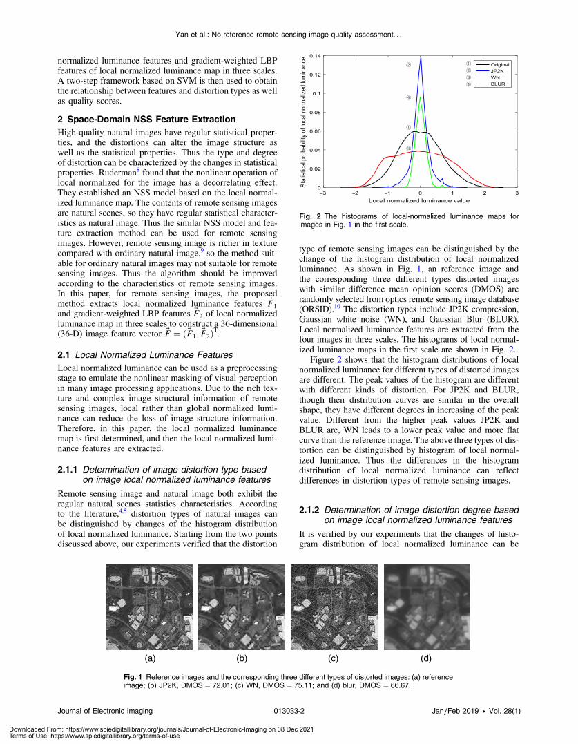
type of remote sensing images can be distinguished by thechange of the histogram distribution of local normalizedluminance. As shown in Fig. 1, an reference image andthe corresponding three different types distorted imageswith similar difference mean opinion scores (DMOS) arerandomly selected from optics remote sensing image database(ORSID).10 The distortion types include JP2K compression,Gaussian white noise (WN), and Gaussian Blur (BLUR).Local normalized luminance features are extracted from thefour images in three scales. The histograms of local normal-ized luminance maps in the first scale are shown in Fig. 2.
Figure 2 shows that the histogram distributions of localnormalized luminance for different types of distorted imagesare different. The peak values of the histogram are differentwith different kinds of distortion. For JP2K and BLUR,though their distribution curves are similar in the overallshape, they have different degrees in increasing of the peakvalue. Different from the higher peak values JP2K andBLUR are, WN leads to a lower peak value and more flatcurve than the reference image. The above three types of dis-tortion can be distinguished by histogram of local normal-ized luminance. Thus the differences in the histogramdistribution of local normalized luminance can reflectdifferences in distortion types of remote sensing images.
2.1.2 Determination of image distortion degree basedon image local normalized luminance features
It is verified by our experiments that the changes of histo-gram distribution of local normalized luminance can be
(a) (b) (c) (d)
Fig. 1 Reference images and the corresponding three different types of distorted images: (a) referenceimage; (b) JP2K, DMOS ¼ 72.01; (c) WN, DMOS ¼ 75.11; and (d) blur, DMOS ¼ 66.67.
Fig. 2 The histograms of local-normalized luminance maps forimages in Fig. 1 in the first scale.
Journal of Electronic Imaging 013033-2 Jan∕Feb 2019 • Vol. 28(1)
Yan et al.: No-reference remote sensing image quality assessment. . .
Downloaded From: https://www.spiedigitallibrary.org/journals/Journal-of-Electronic-Imaging on 08 Dec 2021Terms of Use: https://www.spiedigitallibrary.org/terms-of-use

used to distinguish the different degrees of distortion ofremote sensing images. As shown in Fig. 3, taking WNas an example, a reference image and the five correspondingdistorted images with different degrees of distortion are ran-domly taken from the ORSID. The first-scale local normal-ized luminance histograms of the remote sensing images areshown in Fig. 4. It is shown that with the degree of distortionincreasing (higher DMOS value), the peak value of the histo-gram becomes lower and the curve becomes flatter. Thus thehistogram distribution of local normalized luminance can beused as an indicator of the degree of distortion for remotesensing images.
2.1.3 Extracting image local normalized luminancefeatures
For an image Iðx; yÞ whose size is M × N, after local nor-malized operation of size ð2K þ 1Þ × ð2Lþ 1Þ, the normal-ized luminance at pixel ði; jÞ is defined as4,5
EQ-TARGET;temp:intralink-;e001;326;374I∧ði; jÞ ¼ Iði; jÞ − μði; jÞ
σði; jÞ þ C: (1)
The normalized luminance histogram distribution ofimages can be fitted with a generalized Gaussian distribution(GGD) with mean of zero.8 The zero-mean GGD model isexpressed as follows:
EQ-TARGET;temp:intralink-;e002;326;285fðx; α; σ2Þ ¼ α
2βΓð1∕αÞ exp
�−�jxjβ
�α�: (2)
The parameters α and σ of GGD can represent the distri-bution, therefore α and σ of the normalized luminance histo-gram distribution can represent the character of normalizedluminance. After extracting the normalized luminance map,the BRISQUE method extracts the features using ordinarymoment. In remote sensing images, there are various sceneswith different terrain characteristics and image structures.L-moments can be defined for any random variable whosemean exists, and being linear functions of the data, it suffersless from the effects of sampling variability. Thus L-moments are more robust than conventional moments to out-liers in the data.11–13 So L-moments are used to enhance therobustness for image quality assessment.14 Considering thesereasons, L-moments estimation is used in this paper toenhance the robustness of the proposed method comparingwith that of BRISQUE. On the one hand, L-moments
(a) (b) (c)
(d) (e) (f)
Fig. 3 Reference image and the corresponding five different degrees of WN distorted images: (a) refer-ence image, (b) DMOS ¼ 33.55, (c) DMOS ¼ 37.59, (d) DMOS ¼ 44.60, (e) DMOS ¼ 49.93, and(f) DMOS ¼ 61.94.
Fig. 4 The histograms of local-normalized luminance map for imagesin Fig. 3 in the first scale.
Journal of Electronic Imaging 013033-3 Jan∕Feb 2019 • Vol. 28(1)
Yan et al.: No-reference remote sensing image quality assessment. . .
Downloaded From: https://www.spiedigitallibrary.org/journals/Journal-of-Electronic-Imaging on 08 Dec 2021Terms of Use: https://www.spiedigitallibrary.org/terms-of-use

estimation is insensitive to different scenes of remote sensingimages, and thus robust to parameter estimation of scenes.On the other hand, L-moments estimation is sensitive tothe distortion of different scenes in distorted remote sensingimages, and thus can be used for parameters estimation ofdifferent distortion degrees. For an image normalizedluminance histogram Xi, i ¼ 1; 2; : : : ; n, the first fourL-moments can be expressed as
EQ-TARGET;temp:intralink-;e003;63;557L1 ¼ b0; (3)
EQ-TARGET;temp:intralink-;e004;63;527L2 ¼ 2b1 − b0; (4)
EQ-TARGET;temp:intralink-;e005;63;502L3 ¼ 6b2 − 6b1 þ b0; (5)
EQ-TARGET;temp:intralink-;e006;63;477L4 ¼ 20b3 − 30b2 þ 12b1 − b0; (6)
where br denotes the r’th probability-weighted moment andcan be expressed as
EQ-TARGET;temp:intralink-;e007;63;429b0 ¼P
ni¼1 Xi
n; (7)
EQ-TARGET;temp:intralink-;e008;63;388br ¼P
ni¼rþ1
ði−1Þði−2Þ · · · ði−rÞðn−1Þðn−2Þ · · · ðn−rÞXi
n: (8)
The parameter L1 and L3 are zero due to the symmetry ofGGD. Thus in this paper, L2 and L4 are used to characterizethe distribution of local normalized luminance, yielding localnormalized luminance features. For a distorted image, thereare six local normalized luminance parameters can beextracted in three scales. A six-dimensional (6-D) vectorconsists of six parameters, i.e., ~F1 ¼ ðf1; f2; : : : ; f6Þ. Themeanings of the elements in this 6-D vector are shown inTable 1.
2.2 Gradient-Weighted LBP Features of LocalNormalized Luminance Map
The surface of the earth has obvious spatial characteristics,which can be represented by texture in remote sensingimages. Thus remote sensing images usually have morestructural information than ordinary natural images. TheLBP patterns can effectively express image structural fea-tures, such as edges, lines, corners, and spots. The LBPmap can be obtained by processing the local normalizedluminance map using rotation invariant LBP operator. Onthe LBP map, the value 0 stands for bright spot in the dis-torted image, the value 8 stands for flat area or dark spot inthe distorted image, the value (1 to 7) stands for edges ofdifferent curvature.15 Based on the assumption that localnormalized luminance features and LBP features of local
normalized luminance map is independent,15,16 the combina-tion of the two kinds of features can improve the effective-ness of image quality assessment. However, LBP can reflectthe structural information while the histogram of local nor-malized luminance reflecting statistical distribution of imageluminance. Neither of the two can characterize the contrastinformation of the image. Considering the high sensitivity ofcontrast in HVS, contrast information is extracted by weigh-ing the LBP features of local normalized luminance mapusing gradient. The gradient-weighted LBP features oflocal normalized luminance map can express both structuralfeatures and local contrast features of images, thus themethod can be better applied to remote sensing images withcomplex structural information.
2.2.1 Determination of image distortion type basedon gradient-weighted LBP features of localnormalized luminance map
There exist regular natural scenes statistics characteristics inremote sensing images and natural images. The changes ofhistogram distribution of gradient-weighted LBP in localnormalized luminance map can be used to distinguishthe distortion types of natural images.17 According to theabove two points, our experiments verified that the distortiontypes of remote sensing images can be distinguished by thechanges of histogram distribution of gradient-weighted LBPin local normalized luminance map. Using the referenceimage and three different types distorted images in Fig. 1as input, the gradient-weighted LBP histograms of local nor-malized luminance map in the first scale are shown in Fig. 5.
Figure 5 shows that the LBP histogram distribution ofJP2K image is high in the middle and low on both sides.This attributes to the block effect the JP2K caused, whichmakes flat areas become edges, i.e., the statistical probabilityof pixels with LBP values of 2 to 6 significantly increases.On the contrary, the LBP histogram distribution curve of WNis low in the middle and high on both sides due to the factthat WN can increase the bright and dark spots on the image.BLUR distortion can make the data tend to uniformity. Thisis due to though there is reduction of the number of brightand dark spots, the statistical probability of edge points is notchanged significantly. The above three types of distortioncan be distinguished clearly using gradient-weighted LBPhistograms of local normalized luminance map. Thus itcan be concluded that the histogram distribution of gra-dient-weighted LBP of local normalized luminance mapcan be used as an indicator to distinguish the distortiontypes of remote sensing images.
2.2.2 Determination of image distortion degree basedon image gradient-weighted LBP features oflocal normalized luminance map
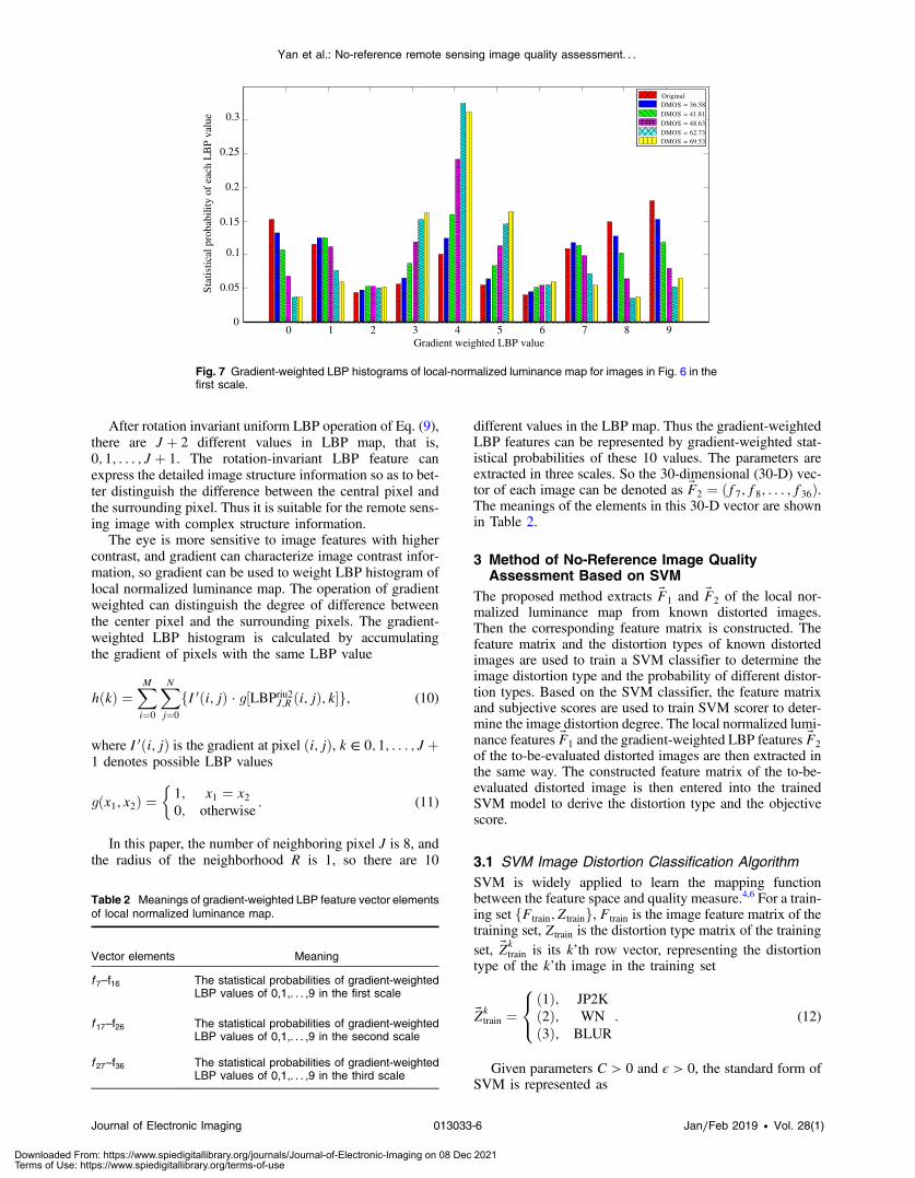
It is verified that the changes of gradient-weighted LBPhistogram distribution of local normalized luminance canbe used to distinguish the different degrees of remote sensingimage distortion according to our experiments. As shown inFig. 6, taking JP2K distortion as an example, a referenceimage and the corresponding five different degrees JP2K dis-torted images are randomly taken from the ORSID database.The first scale local normalized luminance histograms of theimages are shown in Fig. 7. With the degree of JP2K distor-tion increasing (higher DMOS), the blocking artifact
Table 1 Meanings of image local-normalized luminance feature vec-tor elements.
Vector elements Meaning
f 1–f3 The L2 linear moments in three scales
f 4 − f 6 The L4 linear moments in three scales
Journal of Electronic Imaging 013033-4 Jan∕Feb 2019 • Vol. 28(1)
Yan et al.: No-reference remote sensing image quality assessment. . .
Downloaded From: https://www.spiedigitallibrary.org/journals/Journal-of-Electronic-Imaging on 08 Dec 2021Terms of Use: https://www.spiedigitallibrary.org/terms-of-use

becomes severer, the flat areas in the image become edges,the statistical probability of pixels with LBP values of 8decreases, and the statistical probability of pixels withLBP values of 2 to 6 increases. At the same time, withthe increasing severity of JP2K distortion, the blur distor-tion introduced by the block effect exacerbates the decreasein the statistical probability of pixels with LBP values of 1and 8. Thus it can be concluded that the gradient-weighted LBP histogram distribution of local normalizedluminance map can reflect the distortion degrees ofJP2K images.
2.2.3 Extracting image gradient-weighted LBP fea-tures elements of local normalized luminancemap
LBP operation is performed on the local normalized lumi-nance map, which is obtained according to Eq. (1). Thelocal rotation invariant uniform LBP value is defined as17
EQ-TARGET;temp:intralink-;e009;326;113LBPriu2J;R ði; jÞ ¼�P
J−1t¼0 sðgt − gcÞ; if u½LBPJ;Rði; jÞ� ≤ 2
J þ 1; else:
(9)
0 1 2 3 4 5 6 7 8 90
0.05
0.1
0.15
0.2
0.25
0.3
Gradient weighted LBP value
eulavP
BL
hcaefo
ytilibaborplacitsitatS
OriginalJP2KWNBLUR
Fig. 5 Gradient-weighted LBP histograms of local-normalized luminance map for images in Fig. 1 in thefirst scale.
(a) (b) (c)
(d) (e) (f)
Fig. 6 Reference image and the corresponding five different degrees JP2K distorted images: (a) refer-ence image, (b) DMOS ¼ 36.58, (c) DMOS ¼ 41.81, (d) DMOS ¼ 48.63, (e) DMOS ¼ 62.73, and(f) DMOS ¼ 69.53.
Journal of Electronic Imaging 013033-5 Jan∕Feb 2019 • Vol. 28(1)
Yan et al.: No-reference remote sensing image quality assessment. . .
Downloaded From: https://www.spiedigitallibrary.org/journals/Journal-of-Electronic-Imaging on 08 Dec 2021Terms of Use: https://www.spiedigitallibrary.org/terms-of-use
After rotation invariant uniform LBP operation of Eq. (9),there are J þ 2 different values in LBP map, that is,0; 1; : : : ; J þ 1. The rotation-invariant LBP feature canexpress the detailed image structure information so as to bet-ter distinguish the difference between the central pixel andthe surrounding pixel. Thus it is suitable for the remote sens-ing image with complex structure information.
The eye is more sensitive to image features with highercontrast, and gradient can characterize image contrast infor-mation, so gradient can be used to weight LBP histogram oflocal normalized luminance map. The operation of gradientweighted can distinguish the degree of difference betweenthe center pixel and the surrounding pixels. The gradient-weighted LBP histogram is calculated by accumulatingthe gradient of pixels with the same LBP value
EQ-TARGET;temp:intralink-;e010;63;360hðkÞ ¼XMi¼0
XNj¼0
fI 0ði; jÞ · g½LBPriu2J;R ði; jÞ; k�g; (10)
where I 0ði; jÞ is the gradient at pixel ði; jÞ, k ∈ 0; 1; : : : ; J þ1 denotes possible LBP values
EQ-TARGET;temp:intralink-;e011;63;287gðx1; x2Þ ¼�1; x1 ¼ x20; otherwise
: (11)
In this paper, the number of neighboring pixel J is 8, andthe radius of the neighborhood R is 1, so there are 10
different values in the LBP map. Thus the gradient-weightedLBP features can be represented by gradient-weighted stat-istical probabilities of these 10 values. The parameters areextracted in three scales. So the 30-dimensional (30-D) vec-tor of each image can be denoted as ~F2 ¼ ðf7; f8; : : : ; f36Þ.The meanings of the elements in this 30-D vector are shownin Table 2.
3 Method of No-Reference Image QualityAssessment Based on SVM
The proposed method extracts ~F1 and ~F2 of the local nor-malized luminance map from known distorted images.Then the corresponding feature matrix is constructed. Thefeature matrix and the distortion types of known distortedimages are used to train a SVM classifier to determine theimage distortion type and the probability of different distor-tion types. Based on the SVM classifier, the feature matrixand subjective scores are used to train SVM scorer to deter-mine the image distortion degree. The local normalized lumi-nance features ~F1 and the gradient-weighted LBP features ~F2
of the to-be-evaluated distorted images are then extracted inthe same way. The constructed feature matrix of the to-be-evaluated distorted image is then entered into the trainedSVM model to derive the distortion type and the objectivescore.
3.1 SVM Image Distortion Classification AlgorithmSVM is widely applied to learn the mapping functionbetween the feature space and quality measure.4,6 For a train-ing set fFtrain; Ztraing, Ftrain is the image feature matrix of thetraining set, Ztrain is the distortion type matrix of the trainingset, ~Zk
train is its k’th row vector, representing the distortiontype of the k’th image in the training set
EQ-TARGET;temp:intralink-;e012;326;154
~Zktrain ¼
8<:
ð1Þ; JP2K
ð2Þ; WN
ð3Þ; BLUR
: (12)
Given parameters C > 0 and ϵ > 0, the standard form ofSVM is represented as
0 1 2 3 4 6 7 8 90
0.05
0.1
0.15
0.2
0.25
0.3
OriginalDMOS = 36.58DMOS = 41.81DMOS = 48.63DMOS = 62.73DMOS = 69.53
Gradient weighted LBP value
eulavP
BL
hc aefo
y tilibabor plac its ita tS
5
Fig. 7 Gradient-weighted LBP histograms of local-normalized luminance map for images in Fig. 6 in thefirst scale.
Table 2 Meanings of gradient-weighted LBP feature vector elementsof local normalized luminance map.
Vector elements Meaning
f 7–f16 The statistical probabilities of gradient-weightedLBP values of 0,1,. . . ,9 in the first scale
f 17–f26 The statistical probabilities of gradient-weightedLBP values of 0,1,. . . ,9 in the second scale
f 27–f36 The statistical probabilities of gradient-weightedLBP values of 0,1,. . . ,9 in the third scale
Journal of Electronic Imaging 013033-6 Jan∕Feb 2019 • Vol. 28(1)
Yan et al.: No-reference remote sensing image quality assessment. . .
Downloaded From: https://www.spiedigitallibrary.org/journals/Journal-of-Electronic-Imaging on 08 Dec 2021Terms of Use: https://www.spiedigitallibrary.org/terms-of-use

EQ-TARGET;temp:intralink-;e013;63;752 minω;b;ξ;ξ�
1
2ωTωþ C
�XKk¼1
ξk þXKk¼1
ξ�k
�: (13)
The corresponding constraint conditions are as follows:
EQ-TARGET;temp:intralink-;e014;63;701−ðϵþ ξ�Þ ≤ ωTϕð~FitrainÞ þ b − j~Zk
trainj ≤ ϵþ ξ; (14)
EQ-TARGET;temp:intralink-;e015;63;668ξk; ξ�k ≥ 0; k ¼ 1;2; : : : ; Kl ðI ∈ f1; 2; 3gÞ; (15)
where ω represents the matrix that needs to be trained, andb is a constant of 1. The radial basis function kernelKFð~Fi
train; ~FjtrainÞ ¼ expð−γk~Fi
train − ~FjtrainkÞ is used to re-
present the kernel function KFð~Fitrain; ~F
jtrainÞ ¼
ϕð~FitrainÞTϕð~Fj
trainÞ.Taking training set fFtrain; Ztraing as the input of SVM
classifier. The constructed image feature matrix Ftest ofthe test set is entered into the trained SVM classifier to obtainthe distortion type matrix Tp of the test set images and thedetermination probability T ¼ ðT1; T2; T3Þ of each type ofdistortion.
3.2 SVR Image Quality Score AlgorithmThe SVR image quality score algorithm is basically the sameas the SVM image distortion classification algorithm men-tioned above except for the form of the input and the output.Taking fF1
train; Z1traing, fF2
train; Z2traing, fF3
train; Z3traing as input,
the three SVR scorers for JP2K, WN and BLUR distortionare trained, respectively. After obtaining the trained SVRscorers, the constructed image feature matrix Ftest in thetest set is entered into the trained SVR scorers to obtainobjective quality scores S ¼ ðS1; S2; S3Þ of each type of dis-tortion, the image quality objective quality score Sp isobtained using weighted probability of distortion type.
4 Experimental Results and AnalysisTo illustrate the subjective consistency of the proposedGWNSS method, experiments of the proposed GWNSS andother existing IQA methods are performed on the ORSIDdatabase,10 the LIVE database,18,19 and the LIVEMD data-base,20 respectively. The subjective consistency performanceof GWNSS is verified by four indices, which are root-mean-squared error (RMSE), Pearson linear correlation coef-ficient (PLCC), Spearman rank order correlation coefficient(SROCC), and Kendall rank order correlation coefficient(KROCC). In order to verify that the performance ofGWNSS is not restricted to a specific database, the databaseindependence experiments are performed on the LIVE andTID2013 database,21 and SROCC is used as the evaluationindex. All experiments were performed on a Lenovo desktopcomputer, which has an Intel core i3-2130 processor with4 GB memory and 3.4G frequency. The operating systemis win7, and the experimental platform is MATLAB R2015a.
4.1 Comparison of GWNSS Performance inOne-Step and Two-Steps Framework
In this paper, a one-step framework, which is similar to thatproposed in Ref. 3, is also investigated. In this approach, thefeatures extraction is the same as the two-steps framework.Instead of using SVM classifier and SVR scorer, the one-stepframework directly constructs the SVR scorer using all dis-torted image feature matrix and subjective score matrix in
the training set as training data. As shown in Table 3,SROCC of one-step GWNSS is slightly lower than that ofthe two-steps GWNSS. The reason is that under the two-steps framework, different parameters can be selected foreach SVM scorer for different distortion types. Thus eachSVR scorer can more accurately predict the correspondingdistortion type. However, under the one-step framework,the parameter that the SVR scorer selected is an excellentparameter for all types of distorted images in the trainingset instead of optimum parameter for specific distortion type.
4.2 Comparison of Subjective Consistency withOther Objective IQA Methods in the ORSIDDatabase
The subjective consistency performance of the four FR-IQAmethods [peak signal-to-noise ratio (PSNR), structural sim-ilarity index (SSIM),22 feature similarity index (FSIM),23 andvisual information fidelity (VIF)24] and the six NR-IQAmethods [BLIINDS-II,2 BRISQUE,4,5 SSEQ,3 blind imagequality assessment metric based on high order derivatives(BHOD),25 blind image quality assessment (BIQA),26 andNRSL6] for images of three distortion types in the ORSIDdatabase are shown in Table 4. The performance of theGWNSS is compared with those of the abovementioned10 IQA methods. The subjective consistency performanceis assessed by four indices, which are SROCC, PLCC,KROCC, and RMSE. The experiments are repeated 1000times to obtain the median of the subjective consistency per-formance. In Table 4, the top three correlation indices withineach distortion category are marked in bold and the best cor-relation indices are highlighted with the standard red color.
Table 4 shows that the proposed GWNSS and the state-of-the-art methods NRSL and BIQA have high subjective con-sistency. The performance of the 11 methods for 3 types ofdistorted images is evaluated by 4 correlation coefficientindices, yielding 12 indices for per method. The proposedGWNSS method has 12 indices in the top 3 and 8 indicesin the top 1. BIQA and NRSL have 8 and 7 out of 12 indicesin the top 3, respectively. Taking all distortion images in theORSID database together, all four correlation coefficientindices of the proposed GWNSS method are the bestamong all IQA methods. The proposed GWNSS methodachieves good assessment results for all types of distortionand thus exhibits high robustness for different distortions.The proposed GWNSS, even when compared with theFR-IQA methods, still shows relatively high subjective con-sistency. The performance of GWNSS is superior to PSNR,SSIM, FSIM, and VIF methods.
The scatter plots of the subjective and objective consis-tency scores of four well-performing methods, which areGWNSS, BRISQUE, NRSL, and BIQA, are shown in Fig. 8.The x axis denotes the objective score obtained by the image
Table 3 The subjective consistency comparison of the GWNSSmethods under the one-step framework and under the two-stepframeworks for all distorted images in the ORSID database.
JP2K WN BLUR ALL
GWNSS (one-step) 0.9336 0.9278 0.9444 0.9385
GWNSS (two-step) 0.9594 0.9338 0.9669 0.9429
Journal of Electronic Imaging 013033-7 Jan∕Feb 2019 • Vol. 28(1)
Yan et al.: No-reference remote sensing image quality assessment. . .
Downloaded From: https://www.spiedigitallibrary.org/journals/Journal-of-Electronic-Imaging on 08 Dec 2021Terms of Use: https://www.spiedigitallibrary.org/terms-of-use

quality assessment method and the y axis denotes the sub-jective score obtained by human eyes. Figure 8 shows thatthe scatter points of GWNSS, BRISQUE, NRSL, and BIQAare concentrated close to the fitting curves, indicating highobjective–subjective consistency.
4.3 Comparison of Subjective Consistency withOther Objective IQA Methods in the LIVEDatabase and the LIVEMD Database.
There are 29 different reference images and 779 distortedimages in the LIVE database. The distortion types includeJP2K, JPEG, WN, BLUR, and fast fading (FF), and the sub-jective DMOS of distorted images are given as well. Thereare 15 different reference images and 450 multiply distortedimages in the LIVEMD database. The distortion typesinclude BLUR followed by JPEG (BJ) and BLUR followedby noise (BN). The subjective DMOS of multiply distortedimages are given as well.
The subjective consistency performance of the four FR-IQA methods (PSNR, SSIM,22 FSIM,23 and VIF24), the sixNR-IQA methods (BLIINDS-II,2 BRISQUE,4,5 SSEQ,3
BHOD,25 BIQA,26 and NRSL6), and one deep learning-based method on the use of deep learning for blind IQA(DeepBIQ)27 in the LIVE database is shown in Table 5.The performance indices of these methods in the LIVEMDdatabase are shown in Table 6. 80% of all distorted imagesare randomly selected as the training set and 20% as thetest set. The above experiments are repeated 1000 times toobtain the median of the subjective consistency performance.
Tables 5 and 6 show that the proposed GWNSS methodhas high subjective consistency. The performance of the 11methods for 5 types of distorted images in the LIVE databaseis evaluated by 4 correlation coefficient indices, yielding 20indices for per method. The proposed GWNSS has 16 out of20 indices in the top 3 of respective distortion categories.Taking all distortion images in the LIVEMD databasetogether, all four correlation coefficient indices of the pro-posed GWNSS method are the best among all IQA methods.
Table 4 Comparison of the subjective consistency of different IQAmethods in the ORSID database.
Performance indices Methods JP2K WN BLUR ALL
SROCC PSNR 0.8192 0.9541 0.6807 0.8012
SSIM 0.9032 0.9244 0.8435 0.8765
FSIM 0.9485 0.9367 0.9037 0.8819
VIF 0.9587 0.9579 0.9587 0.9232
BLIINDS-II 0.9338 0.9008 0.9383 0.9225
BRISQUE 0.8617 0.9567 0.9173 0.9173
SSEQ 0.9083 0.9218 0.8992 0.8641
BHOD 0.8767 0.8045 0.9248 0.8331
BIQA 0.9353 0.9338 0.9504 0.9334
NRSL 0.9128 0.9353 0.9459 0.9280
GWNSS 0.9594 0.9347 0.9669 0.9425
PLCC PSNR 0.8427 0.9594 0.7003 0.8018
SSIM 0.9060 0.9275 0.8649 0.8710
FSIM 0.9616 0.9373 0.9274 0.8850
VIF 0.9747 0.9706 0.9720 0.9253
BLIINDS-II 0.9533 0.9124 0.9497 0.9275
BRISQUE 0.8938 0.9747 0.9356 0.9217
SSEQ 0.9083 0.9218 0.8992 0.8641
BHOD 0.9150 0.7908 0.9376 0.8451
BIQA 0.9664 0.9366 0.9615 0.9372
NRSL 0.9345 0.9517 0.9513 0.9300
GWNSS 0.9799 0.9573 0.9750 0.9489
KROCC PSNR 0.6108 0.8158 0.4880 0.5967
SSIM 0.7367 0.7519 0.6513 0.6788
FSIM 0.8108 0.7797 0.7108 0.6815
VIF 0.8316 0.8215 0.8184 0.7421
BLIINDS-II 0.8000 0.7368 0.8000 0.7548
BRISQUE 0.6947 0.8438 0.7579 0.7503
SSEQ 0.7579 0.7684 0.7263 0.6734
BHOD 0.7158 0.6316 0.7757 0.6407
BIQA 0.8000 0.7924 0.8316 0.7763
NRSL 0.7597 0.8307 0.8105 0.7627
GWNSS 0.8526 0.8000 0.8632 0.7944
Table 4 (Continued).
Performance indices Methods JP2K WN BLUR ALL
RMSE PSNR 8.4029 5.2879 9.2354 7.8421
SSIM 5.4992 5.0237 6.4935 6.4477
FSIM 3.5638 4.6823 4.8391 6.1108
VIF 2.9012 3.2343 3.0408 4.9755
BLIINDS-II 3.9108 5.3494 4.0273 4.8948
BRISQUE 5.7471 2.9943 4.5507 5.1060
SSEQ 5.3702 4.6813 5.0498 6.3781
BHOD 5.0897 8.5256 4.4150 7.3328
BIQA 3.2794 4.5785 3.5494 4.5805
NRSL 4.6141 4.0530 4.0827 4.9333
GWNSS 2.5585 4.2127 2.8728 4.1035
Journal of Electronic Imaging 013033-8 Jan∕Feb 2019 • Vol. 28(1)
Yan et al.: No-reference remote sensing image quality assessment. . .
Downloaded From: https://www.spiedigitallibrary.org/journals/Journal-of-Electronic-Imaging on 08 Dec 2021Terms of Use: https://www.spiedigitallibrary.org/terms-of-use

The proposed GWNSS method, even when compared withthe FR-IQA methods, still shows relatively high subjectiveconsistency. The performance of GWNSS is superior toPSNR method, close to SSIM, FSIM, and VIF methodsin the LIVE database and it is superior to PSNR, SSIM,FSIM, and VIF methods in the LIVEMD database.
Taking all distortion images in the LIVE databasetogether, KROCC and RMSE of the proposed GWNSSmethod are the best among all IQA methods. When com-pared with deep learning-based method DeepBIQ, SROCCand PLCC are merely 0.01 less than DeepBIQ. The reason isthat the features extracted by CNN-based method are suffi-cient, leading to a good performance. However, GWNSS ismore efficient than DeepBIQ, which can efficiently extractfeatures and conduct training. In addition, the GWNSS haslow requirement for hardware and can be used in widerapplications.
The scatter plots of the subjective and objective consis-tency scores of GWNSS, BRISQUE, NRSL, and BIQAmethods are shown in Fig. 9. The x axis denotes the objectivescore obtained by the image quality assessment method andthe y axis denotes the subjective score obtained by human
eyes. Figure 9 shows that the scatter points of the abovefour NR-IQA methods are concentrated close to the fittingcurves, indicating high objective–subjective consistency.
4.4 Database Independence ExperimentsTo verify that the performance of GWNSS is not restricted tothe particular database used, database independence experi-ments are performed on the LIVE database and the TID2013database.21 In the TID2013 database, the selected images forindependence experiments are 24 different reference imagesand 480 distorted images with the same 4 common distortioncategories: JP2K, JPEG, WN and BLUR. Distorted imagesin the LIVE database are used to train an SVM model, andthen distorted images, which are selected in the TID2013database, are tested in the trained model. The SROCC isused as the testing index. The subjective consistency perfor-mance of the four FR-IQA methods (PSNR, SSIM,22
FSIM,23 and VIF24) and the six NR-IQA methods(BLIINDS-II,2 BRISQUE,4,5 SSEQ,3 BHOD,25 BIQA,26 andNRSL6) for images of four different distortion types in theTID2013 database are shown in Table 7. Conversely, dis-torted images in the TID2013 database are used to train
Fig. 8 Scatter plots of the subjective and objective consistency scores of GWNSS, BRISQUE, NRSL,and BIQA methods in the ORSID database.
Journal of Electronic Imaging 013033-9 Jan∕Feb 2019 • Vol. 28(1)
Yan et al.: No-reference remote sensing image quality assessment. . .
Downloaded From: https://www.spiedigitallibrary.org/journals/Journal-of-Electronic-Imaging on 08 Dec 2021Terms of Use: https://www.spiedigitallibrary.org/terms-of-use
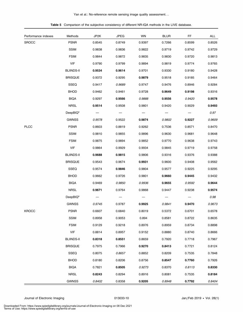
Table 5 Comparison of the subjective consistency of different NR-IQA methods in the LIVE database.
Performance indexes Methods JP2K JPEG WN BLUR FF ALL
SROCC PSNR 0.8545 0.8749 0.9397 0.7266 0.8599 0.8526
SSIM 0.9838 0.9836 0.9822 0.9719 0.9742 0.9729
FSIM 0.9844 0.9872 0.9835 0.9830 0.9720 0.9813
VIF 0.9790 0.9799 0.9894 0.9819 0.9774 0.9765
BLIINDS-II 0.9534 0.9614 0.9701 0.9330 0.9180 0.9428
BRISQUE 0.9372 0.9295 0.9879 0.9518 0.9185 0.9464
SSEQ 0.9417 0.9689 0.9747 0.9476 0.8946 0.9284
BHOD 0.9462 0.9461 0.9728 0.9649 0.9198 0.9316
BIQA 0.9297 0.9566 0.9888 0.9556 0.9420 0.9578
NRSL 0.9514 0.9508 0.9801 0.9420 0.9029 0.9493
DeepBIQa — — — — — 0.97
GWNSS 0.9578 0.9522 0.9874 0.9802 0.9227 0.9609
PLCC PSNR 0.8603 0.8819 0.9262 0.7536 0.8571 0.8470
SSIM 0.9810 0.9855 0.9896 0.9630 0.9681 0.9648
FSIM 0.9875 0.9894 0.9852 0.9770 0.9638 0.9743
VIF 0.9864 0.9929 0.9934 0.9845 0.9719 0.9758
BLIINDS-II 0.9688 0.9815 0.9806 0.9316 0.9376 0.9388
BRISQUE 0.9543 0.9674 0.9931 0.9600 0.9408 0.9562
SSEQ 0.9574 0.9846 0.9804 0.9577 0.9225 0.9295
BHOD 0.9662 0.9726 0.9801 0.9660 0.9445 0.9432
BIQA 0.9469 0.9850 0.9936 0.9655 0.9592 0.9644
NRSL 0.9671 0.9764 0.9868 0.9447 0.9238 0.9574
DeepBIQa — — — — — 0.98
GWNSS 0.9745 0.9787 0.9925 0.9841 0.9470 0.9673
KROCC PSNR 0.6607 0.6840 0.8019 0.5372 0.6701 0.6578
SSIM 0.8958 0.9053 0.894 0.8581 0.8722 0.8635
FSIM 0.9129 0.9218 0.8976 0.8959 0.8734 0.8898
VIF 0.8814 0.8957 0.9152 0.8880 0.8740 0.8666
BLIINDS-II 0.8318 0.8551 0.8659 0.7920 0.7718 0.7967
BRISQUE 0.7975 0.7966 0.9270 0.8413 0.7721 0.8124
SSEQ 0.8075 0.8657 0.8852 0.8209 0.7535 0.7848
BHOD 0.8180 0.8206 0.8756 0.8547 0.7760 0.7926
BIQA 0.7821 0.8505 0.9273 0.8370 0.8113 0.8330
NRSL 0.8243 0.8294 0.8916 0.8081 0.7535 0.8184
GWNSS 0.8402 0.8358 0.9205 0.8948 0.7792 0.8404
Journal of Electronic Imaging 013033-10 Jan∕Feb 2019 • Vol. 28(1)
Yan et al.: No-reference remote sensing image quality assessment. . .
Downloaded From: https://www.spiedigitallibrary.org/journals/Journal-of-Electronic-Imaging on 08 Dec 2021Terms of Use: https://www.spiedigitallibrary.org/terms-of-use
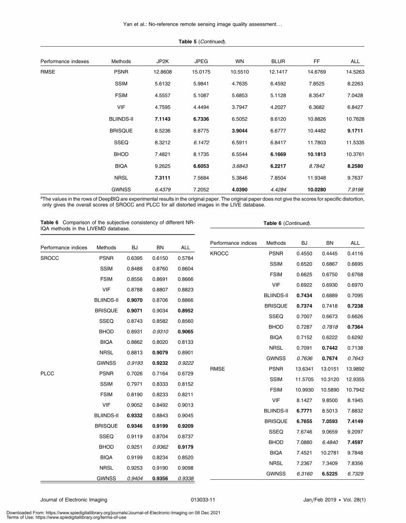
Table 5 (Continued).
Performance indexes Methods JP2K JPEG WN BLUR FF ALL
RMSE PSNR 12.8608 15.0175 10.5510 12.1417 14.6769 14.5263
SSIM 5.6132 5.9841 4.7635 6.4592 7.8525 8.2263
FSIM 4.5557 5.1087 5.6853 5.1128 8.3547 7.0428
VIF 4.7595 4.4494 3.7947 4.2027 6.3682 6.8427
BLIINDS-II 7.1143 6.7336 6.5052 8.6120 10.8826 10.7628
BRISQUE 8.5236 8.8775 3.9044 6.6777 10.4482 9.1711
SSEQ 8.3212 6.1472 6.5911 6.8417 11.7803 11.5335
BHOD 7.4821 8.1735 6.5544 6.1669 10.1813 10.3761
BIQA 9.2625 6.6053 3.6843 6.2217 8.7842 8.2580
NRSL 7.3111 7.5684 5.3846 7.8504 11.9348 9.7637
GWNSS 6.4379 7.2052 4.0390 4.4284 10.0280 7.9198aThe values in the rows of DeepBIQ are experimental results in the original paper. The original paper does not give the scores for specific distortion,only gives the overall scores of SROCC and PLCC for all distorted images in the LIVE database.
Table 6 Comparison of the subjective consistency of different NR-IQA methods in the LIVEMD database.
Performance indices Methods BJ BN ALL
SROCC PSNR 0.6395 0.6150 0.5784
SSIM 0.8488 0.8760 0.8604
FSIM 0.8556 0.8691 0.8666
VIF 0.8788 0.8807 0.8823
BLIINDS-II 0.9070 0.8706 0.8866
BRISQUE 0.9071 0.9034 0.8952
SSEQ 0.8743 0.8582 0.8560
BHOD 0.8931 0.9310 0.9065
BIQA 0.8862 0.8020 0.8133
NRSL 0.8813 0.9079 0.8901
GWNSS 0.9193 0.9232 0.9222
PLCC PSNR 0.7026 0.7164 0.6729
SSIM 0.7971 0.8333 0.8152
FSIM 0.8190 0.8233 0.8211
VIF 0.9052 0.8492 0.9013
BLIINDS-II 0.9332 0.8843 0.9045
BRISQUE 0.9346 0.9199 0.9209
SSEQ 0.9119 0.8704 0.8737
BHOD 0.9251 0.9362 0.9179
BIQA 0.9199 0.8234 0.8520
NRSL 0.9253 0.9190 0.9098
GWNSS 0.9404 0.9356 0.9338
Table 6 (Continued).
Performance indices Methods BJ BN ALL
KROCC PSNR 0.4550 0.4445 0.4116
SSIM 0.6520 0.6867 0.6695
FSIM 0.6625 0.6750 0.6768
VIF 0.6922 0.6930 0.6970
BLIINDS-II 0.7434 0.6889 0.7095
BRISQUE 0.7374 0.7418 0.7238
SSEQ 0.7007 0.6673 0.6626
BHOD 0.7287 0.7818 0.7364
BIQA 0.7152 0.6222 0.6292
NRSL 0.7091 0.7442 0.7138
GWNSS 0.7636 0.7674 0.7643
RMSE PSNR 13.6341 13.0151 13.9892
SSIM 11.5705 10.3120 12.9355
FSIM 10.9930 10.5890 10.7942
VIF 8.1427 9.8500 8.1945
BLIINDS-II 6.7771 8.5013 7.8832
BRISQUE 6.7655 7.0593 7.4149
SSEQ 7.6746 9.0659 9.2097
BHOD 7.0880 6.4840 7.4597
BIQA 7.4521 10.2781 9.7848
NRSL 7.2367 7.3409 7.8356
GWNSS 6.3160 6.5225 6.7329
Journal of Electronic Imaging 013033-11 Jan∕Feb 2019 • Vol. 28(1)
Yan et al.: No-reference remote sensing image quality assessment. . .
Downloaded From: https://www.spiedigitallibrary.org/journals/Journal-of-Electronic-Imaging on 08 Dec 2021Terms of Use: https://www.spiedigitallibrary.org/terms-of-use

an SVMmodel, and then distorted images in the LIVE databaseare tested in the trained model. The subjective consistency per-formance of the four FR-IQAmethods (PSNR, SSIM,22 FSIM,23
and VIF24) and the six NR-IQA methods (BLIINDS-II,2
BRISQUE,4,5 SSEQ,3 BHOD,25 BIQA,26 and NRSL6) forimages of four different distortion types in the LIVE databaseare shown in Table 8. In Tables 7 and 8, the top 3 SROCCindices, within each distortion category, are marked in boldand the best SROCC indices are highlighted with italics.
Tables 7 and 8 show that all 10 indices of the proposedGWNSS method are in the top 3 for four different types ofdistorted images, indicating that the proposed GWNSSmethod achieves high database independence for all fourtypes of distortion. Even comparing with the FR-IQA meth-ods, GWNSS still shows relatively high database independ-ence. The database independence of GWNSS is superior toPSNR method and close to SSIM, FSIM, VIF methods.
4.5 Accuracy of the Distortion Type Judgment of theGWNSS Method
Table 9 shows the accuracy of the GWNSS method in deter-mining the type of image distortion. 80% of all distorted images
are randomly selected as the training set and 20% as the test set,then the training set and the test set are entered into an SVMmodel for training and testing. The above experiment isrepeated 1000 times to obtain the median of the subjective con-sistency performance for the ORSID database. The experimen-tal results show that the GWNSS method is up to 95% accuratein determining the type of image distortion on the wholeORSID database, demonstrating that the GWNSS method per-forms well in classifying the type of image distortion.
The classification performance for different distortion typesin the form of an average confused matrix is shown in Fig. 10.The numerical values are means of the confusion probabilitiesobtained over 1000 experiments. Figure 10 shows that the mostaccurate prediction of the distortion type is WN. As for BLURand JP2K, they confuse with each other, with 0.0479 of theBLUR mistaken as JP2K, and 0.0317 of JP2K mistaken asBLUR. This is because that JP2K can introduce blur intothe image, resulting in confusion with BLUR.
4.6 Time Consumption of the GWNSSSince the runtime of NR-IQA methods is mainly spent onextracting image features, the comparison of mean time
Fig. 9 Scatter plots of the subjective and objective consistency scores of GWNSS, BRISQUE, NRSL,and BIQA methods in the LIVE database and the LIVEMD database.
Journal of Electronic Imaging 013033-12 Jan∕Feb 2019 • Vol. 28(1)
Yan et al.: No-reference remote sensing image quality assessment. . .
Downloaded From: https://www.spiedigitallibrary.org/journals/Journal-of-Electronic-Imaging on 08 Dec 2021Terms of Use: https://www.spiedigitallibrary.org/terms-of-use

spent for feature extraction of all images in the ORSID data-base of the five good performance NR-IQA methods(BLIINDS-II,2 BRISQUE,4,5 SSEQ,3 BIQA,26 and NRSL6)and GWNSS are shown in Table 10. Table 10 shows thatthe mean time spent by the proposed GWNSS method isfar less than that of SSEQ and BLIINDS-II. On average,the proposed GWNSS method only spent 0.1790 s morethan that of the BRISQUE method and 0.2114 s morethan that of the BIQA method. Thus the proposedGWNSS method has high evaluation accuracy and operationefficiency.
5 ConclusionIn this paper, a 36-D image feature vector consists of thelocal normalized luminance features and the gradient-weighted LBP features of local normalized luminancemap in three scales. First, the feature matrix and the corre-sponding distortion type are used to train the SVM classifier.Then on the basis of the SVM classifier, the feature matrixand the corresponding DMOS are used to train the SVRscorer. A series of comparative experiments were carriedout in the ORSID database, the MDORSID database, theLIVE database, the LIVEMD database, and the TID2013database, respectively. Experimental results show that theproposed method has high accuracy in distortion type clas-sification of remote sensing images, high consistency withsubjective scores, and high robustness for different typesof distortions. In addition, the efficacy of the proposedmethod is not restricted to a particular database and the oper-ation efficiency is high. The research of this paper mainly
Table 7 Comparison of the subjective consistency of different NR-IQA methods in the LIVE database (training set) and the TID2013database (test set).
JP2K JPEG WN BLUR ALL
PSNR 0.8904 0.9150 0.9420 0.9661 0.9216
SSIM 0.9489 0.9316 0.8742 0.9704 0.9212
FSIM 0.9579 0.9329 0.9003 0.9590 0.9547
VIF 0.9538 0.9289 0.9302 0.9659 0.9336
BLIINDS-II 0.9458 0.9001 0.7789 0.9077 0.8742
BRISQUE 0.8785 0.9016 0.9008 0.8966 0.8907
SSEQ 0.9108 0.9247 0.8952 0.8935 0.8692
BHOD 0.9155 0.8815 0.7489 0.9148 0.8943
BIQA 0.9446 0.9013 0.9157 0.9029 0.9164
NRSL 0.7779 0.9092 0.8422 0.9094 0.8797
GWNSS 0.9282 0.9028 0.9042 0.9153 0.9284
Table 8 Comparison of the subjective consistency of different NR-IQA methods in the LIVE database (test set) and the TID2013 data-base (training set).
JP2K JPEG WN BLUR ALL
PSNR 0.9041 0.8946 0.9829 0.8073 0.8834
SSIM 0.9838 0.9836 0.9822 0.9719 0.9729
FSIM 0.9844 0.9872 0.9835 0.9830 0.9813
VIF 0.9790 0.9799 0.9894 0.9819 0.9765
BLIINDS-II 0.9404 0.9277 0.9641 0.8959 0.9348
BRISQUE 0.9178 0.9354 0.9306 0.9182 0.9297
SSEQ 0.9252 0.9343 0.8632 0.8053 0.8087
BHOD 0.9273 0.9236 0.9444 0.9036 0.9050
BIQA 0.9291 0.9185 0.9872 0.8093 0.9260
NRSL 0.9300 0.9355 0.9701 0.8408 0.9130
GWNSS 0.9401 0.9426 0.9746 0.9259 0.9282
Table 9 Accuracy of the distortion type judgment of the GWNSSmethod in the ORSID database.
JP2K WN BLUR ALL
Accuracy (%) 95 95 95 95
Fig. 10 Accuracy of the distortion type judgment of the GWNSSmethod in the ORSID database.
Table 10 Mean time spent extracting all images features by differentNR-IQA methods in the ORSID database.
SSEQ BLIINDS-II BRISQUE BIQA NRSL GWNSS
Meantime (s)
2.9752 82.3711 0.1498 0.1174 0.3297 0.3288
Journal of Electronic Imaging 013033-13 Jan∕Feb 2019 • Vol. 28(1)
Yan et al.: No-reference remote sensing image quality assessment. . .
Downloaded From: https://www.spiedigitallibrary.org/journals/Journal-of-Electronic-Imaging on 08 Dec 2021Terms of Use: https://www.spiedigitallibrary.org/terms-of-use

focuses on single-distorted images. Assessment of multiplydistorted images, which is of more practical significance,will be addressed in the future research.
AcknowledgmentsThis work was supported by the National Natural ScienceFoundation of China (Nos. 61471194 and 61705104),Science and Technology on Avionics IntegrationLaboratory and Aeronautical Science Foundation of China(No. 20155552050), and the Natural Science Foundationof Jiangsu Province (No. BK20170804).
References
1. A. K. Moorthy and A. C. Bovik, “A two-step framework for construct-ing blind image quality indices,” IEEE Signal Process. Lett. 17(5), 513–516 (2010).
2. M. A. Saad, A. C. Bovik, and C. Charrier, “Blind image quality assess-ment: a natural scene statistics approach in the DCT domain,” IEEETrans. Image Process. 21(8), 3339–3352 (2012).
3. L. Liu et al., “No-reference image quality assessment based on spatialand spectral entropies,” Signal Process.: Image Commun. 29(8), 856–863 (2014).
4. A. Mittal, A. K. Moorthy, and A. C. Bovik, “No-reference image qualityassessment in the spatial domain,” IEEE Trans. Image Process. 21(12),4695–4708 (2012).
5. A. Mittal, A. K. Moorthy, and A. C. Bovik, “Blind/reference less imagespatial quality evaluator,” in IEEE Record of the Forty Fifth AsilomarConf. Signals Syst. Comput., pp. 723–727 (2011).
6. Q. Li et al., “Blind image quality assessment using statistical structuraland luminance features,” IEEE Trans. Multimedia 18(12), 2457–2469(2016).
7. L. Liu et al., “Blind image quality assessment by relative gradient sta-tistics and adaboosting neural network,” Signal Process. ImageCommun. 40(C), 1–15 (2016).
8. D. L. Ruderman, “The statistics of natural images,” Network Comput.Neural Syst. 5(4), 517–548 (1994).
9. B. Li, R. Yang, and H. Jiang, “Remote-sensing image compressionusing two-dimensional oriented wavelet transform,” IEEE Trans.Geosci. Remote Sens. 49(1), 236–250 (2011).
10. J. Yan et al., “Remote sensing image quality assessment based on theratio of spatial feature weighted mutual information,” J. Imaging Sci.Technol. 62(2), 0205051 (2018).
11. J. R. Hosking, “L-moments: analysis and estimation of distributionsusing linear combinations of order statistics,” J. R. Stat. Soc. 52(1),105–124 (1990).
12. J. R. Hosking, “Moments or L moments? An example comparing twomeasures of distributional shape,” Am. Stat. 46(3), 186–189 (1992).
13. J. R. Hosking, “On the characterization of distributions by their L-moments,” J. Stat. Plann. Inference 136(1), 193–198 (2006).
14. A. Mittal, A. K. Moorthy, and A. C. Bovik, “Making image qualityassessment robust,” in Conf. Record Forty Sixth Asilomar Conf.Signals, Syst. and Comput., IEEE, pp. 1718–1722 (2015).
15. T. Ojala, M. Pietikäinen, and T. Mäenpää, “Multiresolution gray-scaleand rotation invariant texture classification with local binary patterns,”IEEE Trans. Pattern Anal. Mach. Intell. 24(7), 971–987 (2002).
16. T. Ojala et al., “Texture discrimination with multidimensional distribu-tions of signed gray level differences,” Pattern Recognit. 34(3), 727–739 (2001).
17. Q. Li, W. Lin, and Y. Fang, “No-reference quality assessment for multi-ply-distorted images in gradient domain,” IEEE Signal Process. Lett.23(4), 541–545 (2016).
18. H. R. Sheikh et al., “A statistical evaluation of recent full reference qual-ity assessment algorithms,” IEEE Trans. Image Process. 15(11), 3440–3451 (2006).
19. H. R. Sheikh, M. F. Sabir, and A. C. Bovik, “A statistical evaluation ofrecent full reference image quality assessment algorithms,” IEEE Trans.Image Process. 15(11), 3440–3451 (2006).
20. D. Jayaraman et al., “Objective quality assessment of multiply distortedimages,” in Conf. Record of the Forty Sixth Asilomar Conf. Signals,Syst. and Comput., IEEE, pp. 1693–1697 (2012).
21. N. Ponomarenko et al., “Color image database TID2013: peculiaritiesand preliminary results,” in Proc. 4th Europian Workshop on Visual Inf.Process. EUVIP2013, pp. 106–111 (2013).
22. Z. Wang et al., “Image quality assessment: from error visibility to struc-tural similarity,” IEEE Trans. Image Process. 13(4), 600–612 (2004).
23. L. Zhang et al., “FSIM: a feature similarity index for image qualityassessment,” IEEE Trans. Image Process. 20(8), 2378–2386 (2011).
24. H. R. Sheikh and A. C. Bovik, “Image information and visual quality,”in Proc. IEEE Int. Conf. Acoust. Speech Signal Process., IEEE, Vol. 3(2004).
25. Q. Li, W. Lin, and F. Fang, “No-reference image quality assessmentbased on high order derivatives,” in IEEE Int. Conf. Multimedia andExpo, IEEE, pp. 1–6 (2016).
26. W. Xue et al., “Blind image quality assessment using joint statistics ofgradient magnitude and Laplacian features,” IEEE Trans. ImageProcess. 23(11), 4850–4862 (2014).
27. S. Bianco et al., “On the use of deep learning for blind image qualityassessment,” Signal Image Video Process. 12, 355–362 (2018).
Junhua Yan received her BSc, MSc, and PhD degrees from NanjingUniversity of Aeronautics and Astronautics in 1993, 2001, and 2004,respectively. She is a professor at Nanjing University of Aeronauticsand Astronautics. She has been an academic visitor at the Universityof Sussex (October 31, 2016 to October 30, 2017). She is the authorof more than 40 journal papers and has 5 patents. Her currentresearch interests include image quality assessment, multisourceinformation fusion, target detection, tracking, and recognition.
Xuehan Bai is a graduate student at Nanjing University ofAeronautics and Astronautics. Her research interest is image qualityassessment. She received her BSc degree from Harbin Institute ofTechnology in 2016.
Yongqi Xiao received his BSc and MSc degrees from NanjingUniversity of Aeronautics and Astronautics in 2015 and 2018, respec-tively. His research interest is image quality assessment.
Yin Zhang is a lecturer at Nanjing University of Aeronautics andAstronautics. He received his BSc degree in optical information sci-ences and technology from Jilin University in 2009, his MSc and PhDdegrees from Harbin Institute of Technology in 2011 and 2016,respectively. He is the author of more than 10 journal papers andhas 7 patents. His current research interests include remote-sensinginformation processing, image quality assessment, and radiationtransfer calculation.
Xiangyang Lv is a graduate student at Nanjing University ofAeronautics and Astronautics. His research interest is image qualityassessment. He received his BSc degree from Nanjing University ofAeronautics and Astronautics in 2018.
Journal of Electronic Imaging 013033-14 Jan∕Feb 2019 • Vol. 28(1)
Yan et al.: No-reference remote sensing image quality assessment. . .
Downloaded From: https://www.spiedigitallibrary.org/journals/Journal-of-Electronic-Imaging on 08 Dec 2021Terms of Use: https://www.spiedigitallibrary.org/terms-of-use