nmr studies of supercritical co2 in carbon
TRANSCRIPT

NMR STUDIES OF SUPERCRITICAL CO2 IN CARBON
SEQUESTRATION AND IMMISCIBLE TWO
PHASE FLOW IN POROUS MEDIA
by
Cody Allen Prather
A thesis submitted in partial fulfillment
of the requirements for the degree
of
Master of Science
in
Mechanical Engineering
MONTANA STATE UNIVERSITY
Bozeman, Montana
May 2015

©COPYRIGHT
by
Cody Allen Prather
2015
All Rights Reserved

ii
ACKNOWLEDGEMENTS
I would like to acknowledge my family for their unwavering support and
encouragement and my wife, Kyllie Smith, for being there every step of the way. I would
also like to thank my colleagues within the MRM lab for their advice, assistance, and
friendship. Finally, I would like to recognize my mentors, Dr. Sarah Codd and Dr. Joseph
Seymour, for giving me such a wonderful opportunity and for their exceptional guidance
and scientific inspirations.

iii
TABLE OF CONTENTS
1. INTRODUCTION AND BACKGROUND ................................................................... 1
Trapping Mechanisms .................................................................................................... 2 Solubility Trapping (Viscous Fingering Phenomena) ............................................ 4 Capillary Trapping .................................................................................................. 5
2. NUCLEAR MAGNETIC RESONANCE THEORY ..................................................... 8
Introduction to Nuclear Magnetic Resonance (NMR) ................................................... 8
Spin Physics ................................................................................................................... 8
Excitation ..................................................................................................................... 10
Laboratory Frame of Reference ............................................................................ 11 Rotating Frame of Reference ................................................................................ 12
Detection ...................................................................................................................... 14
Faraday’s Law of Induction .................................................................................. 14 Fourier Transforms ............................................................................................... 15
Quadrature Detection ............................................................................................ 17 Discrete Fourier Transform................................................................................... 20
Relaxation ..................................................................................................................... 20
Longitudinal Relaxation........................................................................................ 20 Transverse Relaxation ........................................................................................... 21
Bloch Equations .................................................................................................... 25 Basic Pulse Sequences and Spin Manipulation ............................................................ 25
Signal Averaging .................................................................................................. 25 Phase Cycling........................................................................................................ 26
Spin Echo .............................................................................................................. 28 CPMG ................................................................................................................... 29
Inversion Recovery ............................................................................................... 30 Gradients and K-space ................................................................................................. 31
Gradients ............................................................................................................... 31 K-space ................................................................................................................. 33 ZTE ....................................................................................................................... 37
Selective Excitation .............................................................................................. 38 Translational Motion .................................................................................................... 40
PGSE ..................................................................................................................... 44 Q-Space and Propagators ...................................................................................... 46
3. ZTE SEQUENCE OPTIMIZATION ........................................................................... 51
Introduction .................................................................................................................. 51 Parameter Manipulation ............................................................................................... 52 Image Reconstruction and Analysis ............................................................................. 55

iv
TABLE OF CONTENTS - CONTINUED
Phantom Resolution Experiments ................................................................................ 56 Introduction ........................................................................................................... 56 Experimental Setup and Procedure ....................................................................... 56 Results and Discussion ......................................................................................... 57
Conclusions ........................................................................................................... 60
4. T1 AND T2 PRESSURE DEPENDENCE STUDY .................................................... 61
Introduction .................................................................................................................. 61 Experimental Setup and Procedure .............................................................................. 61
Setup ..................................................................................................................... 61 Procedure .............................................................................................................. 63
Pulse Sequences .................................................................................................... 63 Results and Discussion ................................................................................................. 64
Conclusions .................................................................................................................. 66
5. VISCOUS FINGERING EXPERIMENTS .................................................................. 67
Introduction .................................................................................................................. 67
Experimental Setup and Procedure .............................................................................. 68 Setup ..................................................................................................................... 68
Procedure .............................................................................................................. 69 Pulse Sequences .................................................................................................... 71
Results and Discussion ................................................................................................. 73 Imaging of CO2 Pulse through Saturated Rock Core............................................ 73
Viscous Fingering Experiment ............................................................................. 75 Conclusions and Future Work ...................................................................................... 81
6. CAPILLARY TRAPPING EXPERIMENTS .............................................................. 83
Introduction .................................................................................................................. 83 Experimental Setup and Procedure .............................................................................. 83
Setup ..................................................................................................................... 83 Procedure .............................................................................................................. 85
Pulse Sequences .................................................................................................... 87 Results and Discussion ................................................................................................. 88
AFLAS and FEP Sleeves ...................................................................................... 88 ZTE Data ............................................................................................................... 91 T2 Distribution Data ............................................................................................. 99 5mm Core T2 Distribution Data ......................................................................... 103
Conclusions and Future Work .................................................................................... 105 Future Work ........................................................................................................ 106

v
TABLE OF CONTENTS - CONTINUED
7. TWO PHASE FLOW EXPERIMENT ...................................................................... 108
Introduction ................................................................................................................ 108 Experimental Setup and Procedure ............................................................................ 110
Setup ................................................................................................................... 110 Procedure ............................................................................................................ 111
Pulse Sequences .................................................................................................. 111
Results and Discussion ............................................................................................... 113
NMR Data ........................................................................................................... 116 Conclusions and Future Work .................................................................................... 123
Future Work ........................................................................................................ 123
REFERENCES CITED ................................................................................................... 125
APPENDICES ................................................................................................................ 129
APPENDIX A: ZTE Optimization Data .................................................................... 130
APPENDIX B: T1 and T2 Pressure Dependence Data .............................................. 133 APPENDIX C: Viscous Fingering Data .................................................................... 136 APPENDIX D: Capillary Trapping Data ................................................................... 140
APPENDIX E: Two Phase Flow Data ....................................................................... 164

vi
LIST OF FIGURES
Figure Page
1: CO2 emissions from fossil fuels.......................................................................... 2
2: Stratigraphic trapping ......................................................................................... 3
3: Viscous fingering regimes and numerical simulation
reproduced from [12] .......................................................................................... 5
4: Residually trapped CO2 in rock pores ................................................................. 7
5: Nuclei angular momentum and precession ......................................................... 9
6: Spin state distribution ....................................................................................... 10
7: Evolution of magnetization (lab reference frame) ............................................ 12
8: Evolution of magnetization (rotating reference frame) .................................... 13
9: Electromagnetic induction in a solenoid ........................................................... 14
10: Precession of magnetization in solenoid ......................................................... 15
11: FT addition theorem........................................................................................ 16
12: Quadrature detection scheme .......................................................................... 17
13: Real and imaginary signal and spectrum ........................................................ 19
14: Longitudinal relaxation ................................................................................... 21
15: Transverse relaxation ...................................................................................... 22
16: Relaxation vs. molecular tumbling rate .......................................................... 23
17: Phase cycling representation ........................................................................... 27
18: Spin-echo sequence and spin manipulations .................................................. 28
19: CPMG pulse sequence with echo envelope .................................................... 29

vii
LIST OF FIGURES - CONTINUED
Figure Page
20: Inversion recovery pulse sequence and spin manipulations ........................... 30
21: Tube of water with and without gradients applied ......................................... 32
22: Evolution of spin phase under the application of a gradient........................... 33
23: Pure 2D phase encoding sequence with k-space trajectory ............................ 35
24: Read and phase encoding 2D sequence with k-space trajectory .................... 36
25: Three dimensional ZTE pulse sequence used in experiments ........................ 38
26: Linear magnetic field gradient with position dependent ω ............................. 40
27: Gradient echo sequence depicting the evolution of spins ............................... 41
28: Spin echo sequence with gradient pulses and effective gradient .................... 42
29: Uncompensated (top) and compensated (bottom) gradients ........................... 44
30: PGSE sequence ............................................................................................... 45
31: Diffusion Propagator....................................................................................... 49
32: Three dimensional ZTE pulse sequence with hard RF pulse.......................... 52
33: Background subtraction for ZTE images ........................................................ 56
34: Signal intensity vs. position for 3 rubber phantom samples ........................... 58
35: Signal intensity vs. position for 6.3mm phantom sample ............................... 58
36: Signal intensity vs. position for 3.15mm phantom sample ............................. 59
37: Signal intensity vs. position for 1.68mm phantom sample ............................. 59
38: Experimental setup for pressure dependence study ........................................ 62
39: Pressure versus T2 relaxation for doped DI H2O ........................................... 65

viii
LIST OF FIGURES - CONTINUED
Figure Page
40: Pressure versus T1 relaxation for doped DI H2O ........................................... 66
41: Experimental setup for viscous fingering experiment .................................... 68
42: Multi-slice multi-echo (MSME) pulse sequence ............................................ 72
43: Expectation of 1D ZTE data for CO2 pulse .................................................... 74
44: 1D ZTE data for CO2 front moving through rock core ................................... 74
45: 2D ZTE data for CO2 front moving through rock core ................................... 75
46: Before and after images from pressure inversion incident ............................. 76
47: Relaxation map with red and blue lines indicating where T2
progressions were taken from ......................................................................... 77
48: T2 1D average across length of sample for all 34 scans ................................. 78
49: T2 progression of scans at position 18mm versus time ................................... 78
50: T2 progression of scans at position 62mm versus time ................................... 79
51: 1D average signal intensity vs. position (MSME scans) ................................ 80
52: 1D average signal intensity vs. position (ZTE scans) ..................................... 81
53: Experimental setup and cross section of core holder ...................................... 84
54: T2 distribution comparisons between AFLAS and FEP ................................. 89
55: ZTE images of AFLAS time evolution reaction to CO2 ................................. 90
56: AFLAS sleeve failure ..................................................................................... 91
57: 1D profiles indicating W phase along rock
core length (air/H2O)....................................................................................... 92

ix
LIST OF FIGURES - CONTINUED
Figure Page
58: 1D profiles indicating W phase along rock
core length (CO2/ H2O) ................................................................................... 93
59: 1D profiles indicating W phase along rock
core length (scCO2/ H2O) ................................................................................ 93
60: NW phase initial vs. NW phase residual ........................................................ 99
61: Illustration for defining larger and smaller pores
associated with transverse relaxation times .................................................. 100
62: T2 distribution evolution for drainage/imbibition
of air/water at 75.86bar and ambient temperature ........................................ 101
63: T2 distribution evolution for drainage/imbibition
of CO2/water at 75.86bar and ambient temperature ...................................... 101
64: T2 distribution evolution for drainage/imbibition
of scCO2/water at 75.86bar and 35oC ........................................................... 102
65: T2 distribution comparison of 5mm and 27mm cores .................................. 104
66: Immiscible two phase flow regimes: (a) Bubbly (b) Slug
(c) Froth (d) Annular (e) Dispersed ............................................................. 109
67: Two phase flow setup diagram ..................................................................... 111
68: Example of pressure drop acquisition and steady state (SS) region ............. 113
69: Capillary number vs. pressure gradient (preliminary) .................................. 114
70: Capillary number vs. pressure gradient (recent) ........................................... 115
71: FID data (pressure overlaid) for V = 0.595 ml/min ...................................... 117
72: MSME data (pressure overlaid) for V = 0.595 ml/min ................................ 118
73: FID data (pressure overlaid) for V = 0.188 ml/min ...................................... 121

x
LIST OF FIGURES - CONTINUED
Figure Page
74: MSME data (pressure overlaid) for V = 0.188 ml/min) ............................... 122

xi
LIST OF TABLES
Table Page
1: Phantom FWHM comparison to actual thickness............................................. 60
2: Berea Sandstone Properties .............................................................................. 85
3: Non-wetting phase fraction in Berea rock core #2 ........................................... 95
4: Non-wetting phase fraction in Berea rock core #3 ........................................... 95
5: Average NW phase fractions of all four runs of air, CO2, and scCO2 .............. 97

xii
ABSTRACT
Nuclear magnetic resonance (NMR) was used to research mechanisms related to
two-phase flow in porous media. Experiments were conducted to further understand; 1)
the capillary trapping mechanism that occurs during sequestration of CO2 in deep
underground sandstone reservoirs, 2) the viscous fingering phenomena that occurs when
scCO2 convectively dissolves in brine under reservoir conditions, and 3) flow patterns
and fluid mechanisms in immiscible two-phase flow in porous media for the two pressure
gradient regimes formed under different capillary numbers.
Capillary trapping is a prominent mechanism for initially trapping CO2 in pore
structures of deep underground rock formations during the sequestration process.
Because of its significant role in securing CO2 underground, it is important to
characterize and understand the residual saturation and distribution of CO2 within the
pore structure. A setup was developed in which drainage and imbibition of a Berea
Sandstone core takes place within an NMR spectrometer under reservoir conditions.
NMR results provide comparisons between the different nonwetting fluids used and help
characterize the capillary trapping of each nonwetting fluid. In conclusion, scCO2 is
trapped 13% less efficiently than air or CO2, and the nonwetting fluid is preferentially
trapped in larger pores.
Viscous fingering is a significant long-term trapping mechanism that further
increases storage security by enhancing mass transfer through convective dissolution. A
setup was developed in which scCO2 could dissolve into a water saturated bead pack,
under reservoir conditions, within the NMR spectrometer. NMR results track spatial
changes in T2 relaxation time and signal intensity. The results are inconclusive and the
phenomena could not be directly observed but results do suggest dissolution is occurring
during the experiment.
Immiscible two-phase flow in porous media is unpredictable and existent in many
industries. Therefore, determining flow patterns and understanding the fluid mechanisms
from a capillary number/pressure gradient relationship could prove valuable. A setup was
developed in which an immiscible two-phase flow through a bead pack was monitored,
for different capillary numbers, with NMR techniques. NMR results provide snapshots of
the water saturation distribution within the bead pack. The results suggest there’s a
consistent slug-type flow pattern during the steady state.

1
1. INTRODUCTION AND BACKGROUND
This work presents research utilizing nuclear magnetic resonance (NMR)
techniques to study a dynamic macroscopic system at a laboratory level. NMR is a
versatile tool used to non-invasively study a wide variety of both static and dynamic
systems in many areas of science and is most extensively used in the medical industry,
known in the medical industry as magnetic resonance imaging (MRI). It finds its use in
this thesis with its ability to image fluid transport in porous media in real time and to
extract information regarding pore structure. The primary focus of this thesis is to study
the trapping mechanisms of CO2 when it is pumped into deep underground saline
sandstone reservoirs for secure storage at supercritical conditions.
Anthropogenic CO2 emissions are becoming increasingly prevalent in our society
and the increase in atmospheric concentrations of this greenhouse gas are believed to
contribute to the observed global warming [1]. Figure 1 illustrates the significant
increases in the amount of CO2 emissions from fossil fuels. A currently investigated
viable means of reducing anthropogenic CO2 emissions is through a method called
carbon capture and storage (CCS) [2]. CCS is the process by which CO2 is captured and
securely stored in deep underground saline aquifers or in depleted oil and gas fields.
When CO2 is injected into these deep underground reservoirs it is stored in a supercritical
state. That is, at temperatures and pressures above the critical point of CO2. Supercritical
fluids exhibit both properties of gases and liquids. It has transport properties comparable
to gases and densities similar to liquids [3, 4]. Thus, CO2 in its supercritical state will
have a much larger storage capacity, it’s denser, than in its gaseous state while at the

2
same time enhancing mass transfer, it’s more miscible, and is therefore ideal for geologic
sequestration.
Figure 1: CO2 emissions from fossil fuels1
Trapping Mechanisms
There are four dominant trapping mechanisms that contribute to the long term
storage of CO2: structural trapping (stratigraphic trapping), capillary trapping (residual
trapping), solubility trapping and mineral trapping. Structural trapping is where the
buoyant CO2 plume becomes immobilized underneath an impermeable cap rock,
essentially stopping the upward migration of the CO2 plume from reaching the surface
[5]. This is depicted in the following figure.
1
http://www.iea.org/publications/freepublications/publication/CO2EmissionsFromFuelCombustionHighlight
s2013.pdf
3
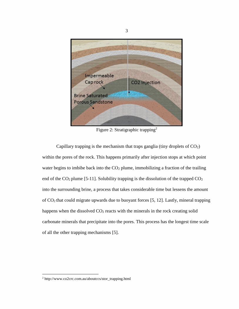
Figure 2: Stratigraphic trapping2
Capillary trapping is the mechanism that traps ganglia (tiny droplets of CO2)
within the pores of the rock. This happens primarily after injection stops at which point
water begins to imbibe back into the CO2 plume, immobilizing a fraction of the trailing
end of the CO2 plume [5-11]. Solubility trapping is the dissolution of the trapped CO2
into the surrounding brine, a process that takes considerable time but lessens the amount
of CO2 that could migrate upwards due to buoyant forces [5, 12]. Lastly, mineral trapping
happens when the dissolved CO2 reacts with the minerals in the rock creating solid
carbonate minerals that precipitate into the pores. This process has the longest time scale
of all the other trapping mechanisms [5].
2 http://www.co2crc.com.au/aboutccs/stor_trapping.html

4
Solubility Trapping (Viscous Fingering Phenomena)
This thesis focuses on two trapping mechanisms, the first being solubility
trapping. Solubility trapping is the result of the residually trapped CO2 dissolving into the
surrounding brine, which further increases the storage security. After CO2 has been
pumped underground into the reservoir it begins to migrate upwards towards to cap rock
due to a greater buoyancy than the brine. The CO2 also begins to dissolve into the
surrounding brine through processes of diffusion and dispersion. As this CO2 dissolves
into the brine it creates a denser layer that at some point becomes unstable and convective
overturning occurs. This is called convective dissolution.
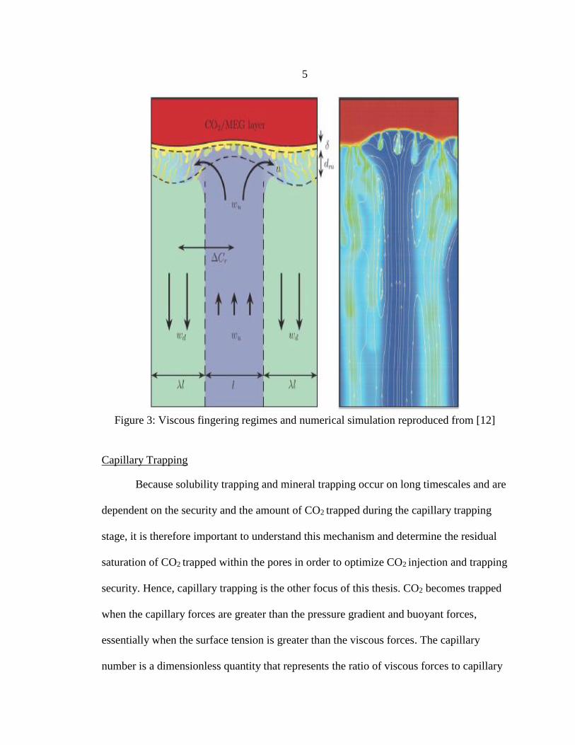
Figure 3 depicts this phenomena of convective dissolution in which downwelling
and upwelling plumes are created, the so called viscous fingering, after the interface
becomes unstable and saturated fingers begin to coalesce. These downwelling plumes of
CO2/brine are denser thus driving the plume downwards. This downward plume increases
the surface area for dissolution thus enhancing the mass transfer, increasing the
dissolution rate. This increase in the dissolution rate further ensures the storage security.
5
Figure 3: Viscous fingering regimes and numerical simulation reproduced from [12]
Capillary Trapping
Because solubility trapping and mineral trapping occur on long timescales and are
dependent on the security and the amount of CO2 trapped during the capillary trapping
stage, it is therefore important to understand this mechanism and determine the residual
saturation of CO2 trapped within the pores in order to optimize CO2 injection and trapping
security. Hence, capillary trapping is the other focus of this thesis. CO2 becomes trapped
when the capillary forces are greater than the pressure gradient and buoyant forces,
essentially when the surface tension is greater than the viscous forces. The capillary
number is a dimensionless quantity that represents the ratio of viscous forces to capillary

6
forces, thus at low capillary numbers the trapping of CO2 occurs. It is defined as equation
[1 where μ is the dynamic viscosity, V is the superficial velocity, and γ is the surface
tension.
𝐶𝑎 =
𝜇𝑉
𝛾 [1]
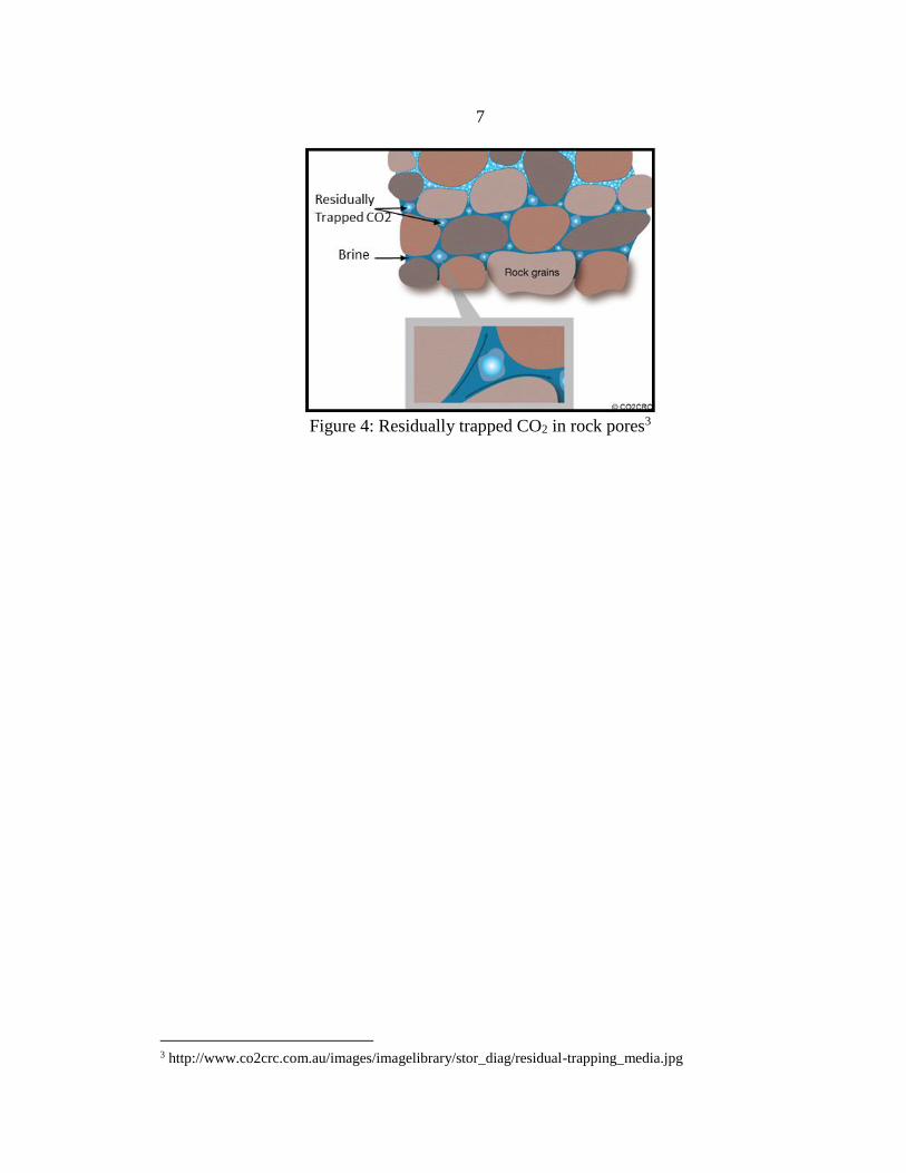
In the case where CO2 is the nonwetting (NW) phase in a deep sandstone saline
aquifer, CO2 ganglia are produced via snap-off at which point it becomes residually
trapped [13]. This is depicted in Figure 4 when an upward migrating plume of CO2 leaves
behind residually trapped ganglia of CO2 via snap-off. Snap-off is an important
phenomena in geologic sequestration because it prevents the separated CO2 ganglia from
continuing to migrate upward with the rest of the plume, reducing the risk of leakage.
Snap-off occurs in the pore throats, a constriction in the pathway, interconnecting larger
pore bodies when a piston-like flow is not possible. Essentially, when the capillary
pressure in the pore throat is greater than the capillary pressure across the NW phase
front in the pore body, snap-off occurs and the NW phase becomes trapped within the
pore body [13-15]. Once trapped the wetting phase fluid, brine in this case, is allowed to
flow around the trapped bubble, indicated in the zoomed in portion of Figure 4.
7
Figure 4: Residually trapped CO2 in rock pores3
3 http://www.co2crc.com.au/images/imagelibrary/stor_diag/residual-trapping_media.jpg

8
2. NUCLEAR MAGNETIC RESONANCE THEORY
Introduction to Nuclear Magnetic Resonance (NMR)
The first evidence of nuclear magnetic resonance was established in 1938 by
Isador Rabi, who through the use of a molecular beam apparatus determined magnetic
moments of nuclei utilizing an oscillating adjustable radio frequency field. NMR was
further expanded by Felix Bloch and Edward Purcell in 1945 for the discovery of nuclear
magnetic resonance in condensed matter, specifically for the hydrogen nuclei [16].
Nuclear magnetic resonance is the phenomena in which electromagnetic radiation is
absorbed and emitted from nuclei when a weaker oscillating magnetic field is applied at a
specific radio frequency in a primary static magnetic field. NMR has come a long way in
the last 75 years and because of its noninvasive techniques has found application in many
areas of science such as chemistry, fluid dynamics, geology, and most predominately in
the medical industry, known as magnetic resonance imaging (MRI). This chapter will
discuss the concepts of NMR and provide an understanding of the tool used in the
experiments presented in this thesis. Most of the information found in this chapter was
obtained from [16] where more detailed information can be found.
Spin Physics
Before understanding how nuclear magnetic resonance (NMR) works it is
important to understand a little about the nuclear spins themselves. The entirety of NMR
is built upon the interactions of the atomic nuclei within static and applied oscillating
magnetic fields. This interaction requires the nuclei to possess a property called spin, or

9
angular momentum. Think of a hydrogen nuclei as our earth with the angular moment
vector being the rotational axis with precession about another axis aligned with the
magnetic field. Our hydrogen nuclei behaves in much the same way within a magnetic
field, B0, as shown in the figure below. As seen from the figure, this precession, or
rotation, may be very hard to see if the angular momentum vector was aligned with the
B0 vector. In order to see this precession, a torque must be applied to the angular
momentum vector rotating it away from the B0 axis.
Figure 5: Nuclei angular momentum and precession
Spin is described by the angular momentum quantum number I. In the Stern-
Gerlach experiment, nuclei’s with I= ½ were found to reside in what is called spin up, ½,
and spin down, -½, states. Nuclear spins impart magnet moments proportional to their
angular momentum vector and spin state. When there are spins outside of a magnetic
field their vectors are oriented randomly and the net magnetic field sums to zero. When a
magnetic field is applied there will be a slight net magnetization along the direction of the
applied magnetic field. Observing a hydrogen nucleus in the presence of a magnetic field,
10
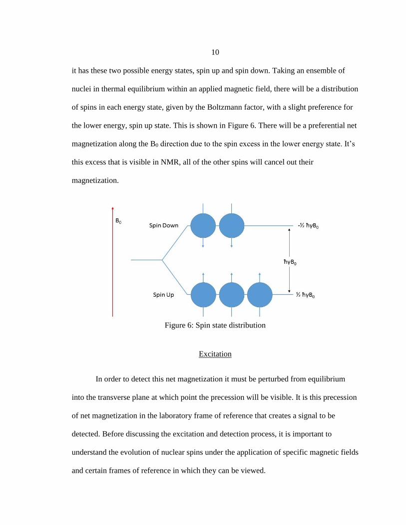
it has these two possible energy states, spin up and spin down. Taking an ensemble of
nuclei in thermal equilibrium within an applied magnetic field, there will be a distribution
of spins in each energy state, given by the Boltzmann factor, with a slight preference for
the lower energy, spin up state. This is shown in Figure 6. There will be a preferential net
magnetization along the B0 direction due to the spin excess in the lower energy state. It’s
this excess that is visible in NMR, all of the other spins will cancel out their
magnetization.
Figure 6: Spin state distribution
Excitation
In order to detect this net magnetization it must be perturbed from equilibrium
into the transverse plane at which point the precession will be visible. It is this precession
of net magnetization in the laboratory frame of reference that creates a signal to be
detected. Before discussing the excitation and detection process, it is important to
understand the evolution of nuclear spins under the application of specific magnetic fields
and certain frames of reference in which they can be viewed.

11
Laboratory Frame of Reference
Starting from the laboratory frame of reference, the net magnetization of spins, as
described by the magnetization vector M, will be in the direction of the applied static
magnetic field, B0. Even though the precession is not visible when the spins are aligned
in the z-direction they are still precessing. This precession frequency is known as the
Larmor frequency, ω0. The Larmor frequency is a function of the gyromagnetic ratio, γ,
and the static magnetic field. It is given by
𝜔0 = 𝛾𝐵0 [2]
In order to tip the magnetization into the transverse plane a torque must be applied
to the magnetization vector. This is achieved by applying a resonant RF magnetic field,
B1, perpendicular to the static B0 field as well as the precessing magnetization vector.
Therefore, B1 must also be applied at the same resonant frequency as the precessional
frequency of the spins, ω0. The effect of this B1 field is to cause the magnetization to
nutate about the B1 axis. Once the B1 field is turned off, the spins now only experience
the effect of the B0 field, this is known as the Zeeman interaction, and are said to be in
free precession, that is, they are simultaneously rotating about the B0 field at their Larmor
frequency while spiraling back to equilibrium along the direction of the static B0 field.
This is illustrated in Figure 7.

12
Figure 7: Evolution of magnetization (lab reference frame)
Rotating Frame of Reference
The rotating frame of reference, that is, the frame of reference in which the x and
y axes are rotating about the z axis at the Larmor frequency, does two helpful things. It
allows the evolution of the magnetization vector to visually be understood better as well
as simplifying some mathematical equations. In this frame of reference the axes are
rotating about the z axis at the Larmor frequency where effectively the longitudinal B0
field is zero and the B1 field appears stationary as long as everything is on resonance, that
is, when ω = ω0. This can be more clearly seen by looking at the Hamiltonian in the
rotating frame of reference defined as
13
𝐻𝑟𝑜𝑡 = −𝛾(𝐵0 − 𝜔 (𝛾)𝐼𝑧⁄ − 𝛾𝐵1𝐼𝑥) [3]
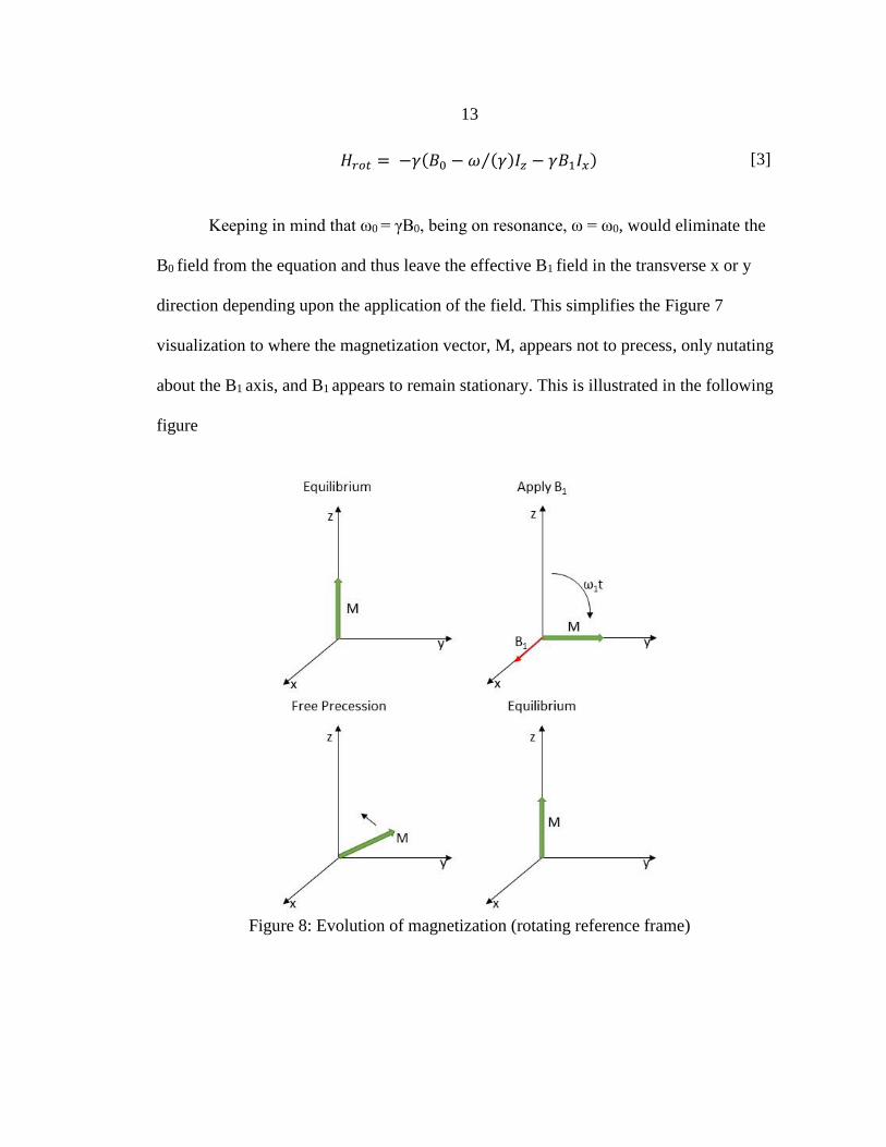
Keeping in mind that ω0 = γB0, being on resonance, ω = ω0, would eliminate the
B0 field from the equation and thus leave the effective B1 field in the transverse x or y
direction depending upon the application of the field. This simplifies the Figure 7
visualization to where the magnetization vector, M, appears not to precess, only nutating
about the B1 axis, and B1 appears to remain stationary. This is illustrated in the following
figure
Figure 8: Evolution of magnetization (rotating reference frame)

14
Detection
Faraday’s Law of Induction
To illustrate how signal is detected it is helpful to imagine the case where the
magnetization is placed in the transverse plane, i.e. a 90o pulse. After the magnetization is
excited and placed into the transverse plane, the RF pulse in turned off and the
magnetization is now in free precession (illustrated in the above figures). This precession
of the magnetization vector at the Larmor frequency about the B0 axis within a radio
frequency coil is what produces a measureable signal, via electromagnetic induction.
Electromagnetic induction is a phenomena in which a voltage is created in a conductor
when it is placed in a varying magnetic field.
Imagine a solenoid, a coil of wire. A magnet is now moved in and out of the coil
of wire. As the magnet moves in, an electromotive force, a voltage, is created which in
turn induces a current in the wire traveling in one direction. As the magnet direction is
changed and removed from the coil of wire, the direction of the induced current in the
wire also reverses direction. This concept is illustrated in the following figure. If a current
is generated in the coil of wires traveling in one direction it will have its corresponding
generated magnetic field lines pointing along one direction within the coil. Now if that
current is reversed, so too do the magnetic field lines within the solenoid.
Figure 9: Electromagnetic induction in a solenoid

15
It is now easy to see that by placing an RF coil near the magnetization vector
while it is precessing at the Larmor frequency that an output signal can be generated.
Referring to the following figure, as the magnetization vector precesses about the B0 axis
it will change direction within the coil therefore creating an oscillating voltage.
Excitation is achieved in a similar manner whereby sending a RF pulse to a coil, it
produces a B1 field in the desired direction nutating the magnetization about its axis. As a
side note, the RF coils depicted here are very simplistic and in reality the RF coils are
quite complex, using a ‘birdcage’ configuration [17].
Figure 10: Precession of magnetization in solenoid
Fourier Transforms
Ignoring relaxation for the moment and imagining the magnetization vector stays
in the transverse plane, i.e. the return to equilibrium via dephasing of spins doesn’t occur,
the output can be written in the form of V(t) = V0cos(ω0t). In order to obtain results that
are meaningful, the output must be Fourier transformed. A Fourier transformation
changes a function from one domain, such as time, to another domain, such as frequency,

16
through the use of integration. It is reversible meaning that it can transform from one
domain to the other and vice versa. It is defined by
S(ω)=F{s(t)}= ∫ s(t)eiωtdt
∞
-∞
[4]
𝑠(𝑡) = 𝐹−1{𝑆(𝜔)} =
1
2𝜋∫ 𝑆(𝜔)𝑒−𝑖𝜔𝑡𝑑𝜔
∞
−∞ [5]
Fourier transforming the cosine will yield a positive and negative frequency of the
same value. The Fourier transform cannot distinguish between the sign of the frequency
based on the data given. So in order to distinguish these frequencies both the Mx and My
transverse magnetization must be obtained and Fourier transformed, that is, the real
(cosine) and imaginary (sine) parts must be obtained and transformed. This will allow a
distinction of frequencies of the same value but with opposite sign. The following figure
illustrates this
Figure 11: FT addition theorem

17
Quadrature Detection
The method employed to obtain both Mx (attributed to real) and My (attributed to
imaginary) is called quadrature detection. Quadrature detection employs mixers and low-
pass filters to obtain the complex difference signal. The output signal voltage is mixed
with two reference signals. One that is in phase and what that is 90o out of phase, also
known as quadrature phase. These signals are then passed through a filter that rejects the
sum frequency terms and keeps the difference terms. The output is now the complex
difference signal and is exactly proportional to that created by the magnetization. The
following figure depicts the quadrature detection scheme.
Figure 12: Quadrature detection scheme
The output can also be written in the form of a complex exponential where
𝑉(𝑡) =
1
2𝑉0 exp(−𝑖(𝜔0𝑡 − 𝜔𝑡))
= 1
2𝑉0 cos(𝜔0𝑡 − 𝜔𝑡) − 𝑖
1
2𝑉0 sin(𝜔0𝑡 − 𝜔𝑡)
[6]
This now allows a distinction between frequencies of opposite sign when Fourier
transformed. If there are any frequencies that are not at the Larmor frequency, ω0, they
18
will show up as an offset frequency from the resonant Larmor frequency, Δω = ω0 – ω.
Thus spin magnetization vectors rotating faster than the Larmor frequency will show up
as a positive offset while spin magnetization vectors rotating slower than the Larmor
frequency will show up as a negative offset. This allows for a distinction of different
frequencies from the Larmor frequency which will show up as different frequencies in a
spectra once Fourier transformed.
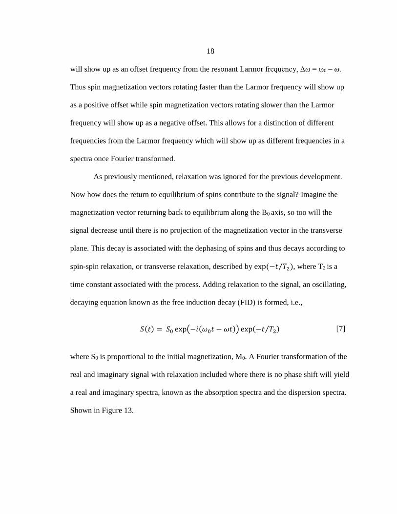
As previously mentioned, relaxation was ignored for the previous development.
Now how does the return to equilibrium of spins contribute to the signal? Imagine the
magnetization vector returning back to equilibrium along the B0 axis, so too will the
signal decrease until there is no projection of the magnetization vector in the transverse
plane. This decay is associated with the dephasing of spins and thus decays according to
spin-spin relaxation, or transverse relaxation, described by exp (−𝑡 𝑇2)⁄ , where T2 is a
time constant associated with the process. Adding relaxation to the signal, an oscillating,
decaying equation known as the free induction decay (FID) is formed, i.e.,
𝑆(𝑡) = 𝑆0 exp(−𝑖(𝜔0𝑡 − 𝜔𝑡)) exp(−𝑡 𝑇2⁄ ) [7]
where S0 is proportional to the initial magnetization, M0. A Fourier transformation of the
real and imaginary signal with relaxation included where there is no phase shift will yield
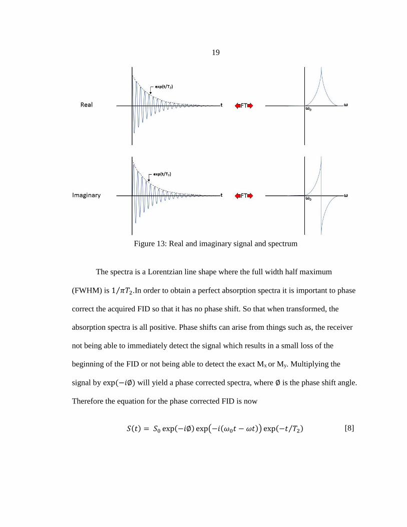
a real and imaginary spectra, known as the absorption spectra and the dispersion spectra.
Shown in Figure 13.
19
Figure 13: Real and imaginary signal and spectrum
The spectra is a Lorentzian line shape where the full width half maximum
(FWHM) is 1 𝜋𝑇2⁄ .In order to obtain a perfect absorption spectra it is important to phase
correct the acquired FID so that it has no phase shift. So that when transformed, the
absorption spectra is all positive. Phase shifts can arise from things such as, the receiver
not being able to immediately detect the signal which results in a small loss of the
beginning of the FID or not being able to detect the exact Mx or My. Multiplying the
signal by exp (−𝑖∅) will yield a phase corrected spectra, where ∅ is the phase shift angle.
Therefore the equation for the phase corrected FID is now
𝑆(𝑡) = 𝑆0 exp(−𝑖∅) exp(−𝑖(𝜔0𝑡 − 𝜔𝑡)) exp(−𝑡 𝑇2⁄ ) [8]

20
The computer does this automatically by observing the absorption spectra and adjusting
∅ until the real absorption spectra becomes all positive and has the maximum integral.
Discrete Fourier Transform
In NMR spectroscopy, the analog signal is digitized for storage in the computer.
Because the computer doesn’t continuously sample the FID but rather it samples in
discrete time points, the discrete Fourier transform is used. This is essentially equivalent
to multiplying the signal by a finite set of delta functions, N number of points, spaced by
a dwell time, dt. It is important to ensure that the sampling frequency, 1 𝑁𝑑𝑡⁄ , is greater
than the FWHM of the spectra or resolution will suffer.
Relaxation
Longitudinal Relaxation
After applying an RF pulse, perturbing the spins from equilibrium along the B0,
the spins will want to return to their equilibrium state because of the dominant Zeeman
interaction. They return to equilibrium via two mechanisms: spin-lattice relaxation and
spin-spin relaxation. The first, spin-lattice relaxation or longitudinal relaxation, as its
name describes, is the return of the magnetization vector to the longitudinal axis along
the B0 field. It is an energy exchange between the spins and their surroundings or lattice.
It is characterized by the equation
𝑑𝑀𝑧
𝑑𝑡= −
𝑀𝑧 − 𝑀0
𝑇1 [9]
which can be solved to yield

21
𝑀𝑧(𝑡) = (𝑀𝑧(0) − 𝑀0)𝑒−𝑡
𝑇1⁄ + 𝑀0
[10]
M0 refers to the equilibrium magnetization along the z-axis in the direction of the
B0 field. In this case, Mz(0) would equal M0 describing the magnetization along the z-
axis. Therefore, Mz describes the longitudinal magnetization. T1 is a time constant that
describes the longitudinal relaxation time. If a 180o RF pulse is applied it will tip the
magnetization into the negative z-axis and thus the Mz magnetization may be plotted in
the following figure according to the equation above.
Figure 14: Longitudinal relaxation
Transverse Relaxation
The other process of spin relaxation is known as spin-spin relaxation or transverse
relaxation. It is the process by which spins come to thermal equilibrium amongst
themselves, hence spin-spin relaxation. It is the decay of the transverse magnetism via the
dephasing of spins, or the loss of coherence of the spins. It is described by the equation
22
𝑑𝑀𝑥𝑦
𝑑𝑡= −
𝑀𝑥𝑦
𝑇2 [11]
which when solved will yield
𝑀𝑥𝑦(𝑡) = 𝑀𝑥𝑦(0)𝑒−𝑡
𝑇2⁄
[12]
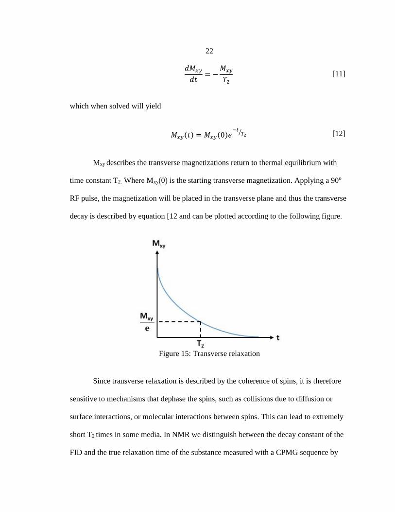
Mxy describes the transverse magnetizations return to thermal equilibrium with
time constant T2. Where Mxy(0) is the starting transverse magnetization. Applying a 90o
RF pulse, the magnetization will be placed in the transverse plane and thus the transverse
decay is described by equation [12 and can be plotted according to the following figure.
Figure 15: Transverse relaxation
Since transverse relaxation is described by the coherence of spins, it is therefore
sensitive to mechanisms that dephase the spins, such as collisions due to diffusion or
surface interactions, or molecular interactions between spins. This can lead to extremely
short T2 times in some media. In NMR we distinguish between the decay constant of the
FID and the true relaxation time of the substance measured with a CPMG sequence by

23
using an asterisk. T2* is the decay constant of the FID that dephases due to field
inhomogeneity.
Because of the additional interactions that contribute to T2 relaxation, T2 will
always be less than or equal to T1. In liquids T1 and T2 can be relatively similar but in
solids T2 is much shorter than T1. Simplistically, this can be visualized and thought of by
plotting the relaxation time vs. the molecular tumbling rate, see Figure 16. The molecular
tumbling rate being related to the size and motion of the molecule. Molecules that are
larger have a slower molecular motion corresponding to the divergence of T1 and T2,
where T2 can be much less than T1. As molecular motion speeds up and molecules
become smaller, as in free water, T1 and T2 are longer and can have similar values.
Figure 16: Relaxation vs. molecular tumbling rate

24
From Bloembergen, Purcell and Pound (BPP) theory, dipolar correlation
functions can be developed for T1 and T2. These dipolar correlation functions are what
describe T1 and T2 in Figure 16. For T1
1
𝑇1= (
𝜇0
4𝜋)
2
𝛾4ℏ23
2𝐼(𝐼 + 1)[𝐽(1)(𝜔0) + 𝐽(2)(2𝜔0)] [13]
And for T2
1
𝑇2= (
𝜇0
4𝜋)
2
𝛾4ℏ23
2𝐼(𝐼 + 1) [
1
4𝐽(0)(0) +
5
2𝐽(1)(𝜔0) +
1
4𝐽(2)(2𝜔0)] [14]
Where
𝐽(0)(𝜔) =
24
15𝑟𝑖𝑗6
𝜏𝑐
1 + 𝜔2𝜏2
𝐽(1)(𝜔) =4
15𝑟𝑖𝑗6
𝜏𝑐
1 + 𝜔2𝜏2
𝐽(2)(𝜔) =16
15𝑟𝑖𝑗6
𝜏𝑐
1 + 𝜔2𝜏2
[15]
for a simple isotropic rotational diffusion model for a pair of like spins, which represent
the dipolar interactions in most liquids. Each 𝐽(𝑖)(𝜔) term describes different dipolar
interactions. A key thing to note is that T2 has one more term than T1 does and thus is
sensitive to more interactions than T1 giving more explanation as to why T2 ≤ T1.

25
Bloch Equations
In order to describe the macroscopic motion of the magnetization three equations
are needed: a description of the longitudinal magnetization and the transverse
magnetization, and the rate of change of angular momentum.
The rate of change of angular momentum is described by
𝑑𝑀
𝑑𝑡= 𝛾𝑀 × 𝐵 [16]
Plugging in equations [9 and [11, a set of coupled differential equations are obtained that
can be used to describe the magnetization vector in the rotating frame of reference. They
are
𝑑𝑀𝑥
𝑑𝑡= 𝛾𝑀𝑦(𝐵0 − 𝜔
𝛾⁄ ) −𝑀𝑥
𝑇2
𝑑𝑀𝑦
𝑑𝑡= 𝛾𝐵1 − 𝛾𝑀𝑥(𝐵0 − 𝜔
𝛾⁄ ) −𝑀𝑦
𝑇2
𝑑𝑀𝑧
𝑑𝑡= −𝛾𝑀𝑦𝐵1 −
𝑀𝑧 − 𝑀0
𝑇1
[17]
Basic Pulse Sequences and Spin Manipulation
Signal Averaging
Due to low signal in NMR it is beneficial to add signal from multiple
experiments. This has the effect that signals will continue to add coherently whereas
random noise will lead to incoherence that starts canceling. This successfully enhances
the signal-to-noise ratio (SNR), distinguishing the signal from the noise. The SNR
improves as N1/2, where N is the number of experiments. Increasing the number of

26
experiments from 1 to 2 doubles the experiment time. The time for the spins to recover
their z-axis magnetization limits the number of experiments that can be added in a certain
amount of time. The repetition time, TR, is how long the experiment waits before
repeating, in which time the magnetization fully recovers. Not allowing a full TR before
repeating the pulse sequence will result in a decrease in signal because the magnetization
was never allowed to reach its maximum equilibrium magnetization and thus the starting
magnetization is less than 100%. A good rule of thumb is to have a TR ≥ 5T1. This will
allow the magnetization to return to equilibrium and full signal strength will be obtained.
Phase Cycling
Phase cycling is a method used to eliminate artifacts due to the electronic
hardware and quantum mechanics complications on the desired pulse sequence pathway.
It is achieved by varying the phase of the pulses and the phase of the receiver in order to
cancel or add certain signals. The phase of the signal is dependent on the phase of the RF
pulse. Therefore signal can be distinguished from the background noise by cycling the
phase of the pulse and receiver in repeated experiments in such a manner that the desired
coherence pathway is additive and all others cancel. Phase cycling can be quite complex
but a simple example will be explained to illustrate the effect of phase cycling.
Amplifiers often have a baseline offset, a DC offset, and to correct for this offset,
without buying a more expensive amplifier, phase cycling is employed. First, a 90x pulse
is applied and then the FID is recorded. Then a 90-x pulse is applied and the FID is
recorded. Note that the receiver does not change phase while the applied RF pulse does.
Finally, the 90-x FID is multiplied by -1 and added to the 90x FID where the signals add
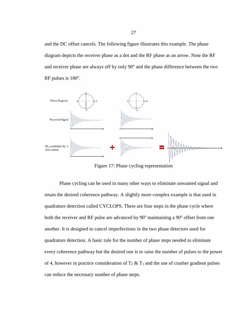
27
and the DC offset cancels. The following figure illustrates this example. The phase
diagram depicts the receiver phase as a dot and the RF phase as an arrow. Note the RF
and receiver phase are always off by only 90o and the phase difference between the two
RF pulses is 180o.
Figure 17: Phase cycling representation
Phase cycling can be used in many other ways to eliminate unwanted signal and
retain the desired coherence pathway. A slightly more complex example is that used in
quadrature detection called CYCLOPS. There are four steps in the phase cycle where
both the receiver and RF pulse are advanced by 90o maintaining a 90o offset from one
another. It is designed to cancel imperfections in the two phase detectors used for
quadrature detection. A basic rule for the number of phase steps needed to eliminate
every coherence pathway but the desired one is to raise the number of pulses to the power
of 4, however in practice consideration of T2 & T1 and the use of crusher gradient pulses
can reduce the necessary number of phase steps.
28
Spin Echo
It is important to understand some basic pulse sequences that are used in NMR.
Many are so common that they have become second nature and are the basics of more
complex pulse sequences. Understanding these sequences that have endured since the
beginning will prove to be valuable and insightful in understanding basic spin
manipulation and provide a crux for the more advanced.
A basic 90o RF pulse and acquisition of the FID have been previously discussed.
The next step in this sequence leads to a sequence called the spin-echo. Magnetic field
inhomogeneity causes dephasing of the transverse magnetization because there is a
spread of Larmor frequencies and thus a loss of phase coherence. The spin-echo causes
these spins to rephase, reversing the loss of phase coherence, which form what is called
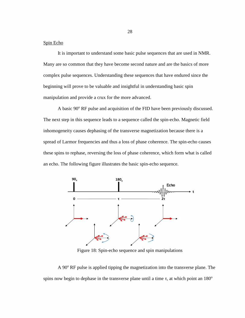
an echo. The following figure illustrates the basic spin-echo sequence.
Figure 18: Spin-echo sequence and spin manipulations
A 90o RF pulse is applied tipping the magnetization into the transverse plane. The
spins now begin to dephase in the transverse plane until a time τ, at which point an 180o

29
RF pulse is applied rotating the spins 180o about the y-axis. This effectively inverts the
phase of each spin. The spins now begin to refocus and at time 2τ a perfect echo is
formed. Capturing the echo will return a signal, that has refocused any dephasing, that
can be Fourier transformed to obtain a spectra that has only attenuated due to T2
relaxation over the time 2τ. The spin-echo sequence essentially removes the effects of
any inhomogeneous dephasing.
CPMG
After a time 2τ the spins continue to dephase and the signal is effectively lost.
However, it can be successively recovered with the application of multiple 180o RF
pulses called a train. Because the effects of spin-spin relaxation are irreversible, they are
the only thing contributing to the attenuation of the echoes. Thus, the envelope created by
multiple spin echoes is determined only by T2 decay. Therefore, the Carr-Purcell-
Meiboom-Gill (CPMG) pulse sequence makes it possible to determine the characteristic
time constant T2. The following figure illustrates the CPMG method.
Figure 19: CPMG pulse sequence with echo envelope

30
The pulse sequence starts the same as the spin-echo sequence but successive 180o
RF pulses are applied at the interval 2nτ-1 and echoes are formed at 2nτ. The echoes are
attenuated due to spin-spin relaxation and therefore an equation for T2 decay can be
written as
𝑀𝑦(𝑡) = 𝑀0𝑒(−𝑡 𝑇2⁄ ) [18]
This describes the envelope of signal from which the characteristic time constant T2 can
be determined.
Inversion Recovery
The inversion recovery pulse sequence is used to determine the characteristic time
constant T1 as well as to suppress unwanted signals by knowing where the null point
occurs (the point at which there is zero magnetization). The following figure depicts this
pulse sequence.
Figure 20: Inversion recovery pulse sequence and spin manipulations
The sequence differs from others in that it starts with an 180o RF pulse that tips
the magnetization into the –z-axis. During some time τ the magnetization relaxes along

31
the longitudinal axis due to spin-lattice relaxation. At a time τ a 90o RF pulse is applied
and tips the remaining magnetization into the transverse plane during which it begins to
dephase resulting in a FID. The magnetization can be described by equation [10. If the τ
time was varied the resulting maximum amplitudes of the various FID’s would create a
curve that is similar to Figure 14. Equation [10 can then be applied to this curve to
determine the time constant T1. Notice at 𝑡 = 0.6931𝑇1 there is a crossover where the
magnetization is equal to zero. This point is known as the null point and is what is
exploited to suppress unwanted signals.
Gradients and K-space
Gradients
In spectral imaging, inhomogeneity in the magnetic field was seen as a nuisance,
where it hindered resolution. Looking at them from a time-domain perspective however,
it’s seen that an echo attenuation is formed based on the time between pulses in which
molecular motion occurs. This molecular motion being dictated by variations in the
magnetic field. The basis of NMR imaging is in this spatially varying magnetic field,
called a magnetic field gradient. The most useful gradient in NMR is a linear magnetic
field gradient. The fundamental principle that makes imaging possible from these linear
magnetic field gradients leads us back to the Larmor equation, 𝜔0 = 𝛾𝐵0. If B0 was
made a function of position, that is, there was a linear magnetic field gradient applied,
then ω0 would also be a function of position and therefore the position of one spin could
be distinguished from another.
32
Applying a gradient in one dimension, according to Maxwell’s equations, would
lead to smaller contributions in the other two dimensions. In high field NMR, it is said
that these smaller contributions are negligible thus leading to the equation
𝜔0(𝒓) = 𝛾𝐵0 + 𝒓 ∙ 𝑮 [19]
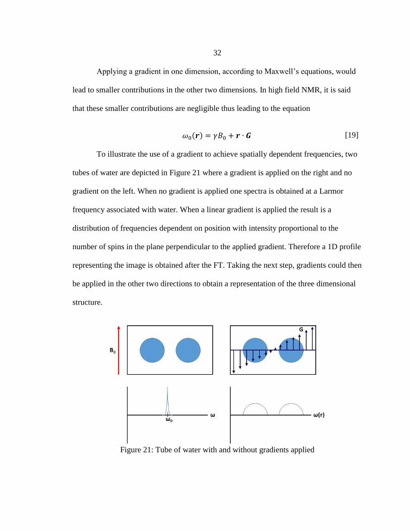
To illustrate the use of a gradient to achieve spatially dependent frequencies, two
tubes of water are depicted in Figure 21 where a gradient is applied on the right and no
gradient on the left. When no gradient is applied one spectra is obtained at a Larmor
frequency associated with water. When a linear gradient is applied the result is a
distribution of frequencies dependent on position with intensity proportional to the
number of spins in the plane perpendicular to the applied gradient. Therefore a 1D profile
representing the image is obtained after the FT. Taking the next step, gradients could then
be applied in the other two directions to obtain a representation of the three dimensional
structure.
Figure 21: Tube of water with and without gradients applied

33
K-space
In order to understand how two and three dimensional images are created it is
necessary to introduce and understand k-space and how pulse sequences traverse k-space.
The spins contribute a transverse magnetization in a rotating frame set on resonance,
ignoring relaxation for simplicity, given by
𝑀(𝒓, 𝑡) = 𝑀(𝒓, 0)𝑒(−𝑖𝛾𝒓∙𝑮𝑡) [20]
Now imagine applying a gradient along the z-axis. The equation then takes the form
𝑀(𝑧, 𝑡) = 𝑀(𝑧, 0)𝑒(−𝑖𝛾𝑧𝐺𝑡) [21]
The evolution of the phase of spins along the z direction take the form of a helix.
The wavelength of the helix will become smaller, it winds up tighter, as either time goes
on or a larger gradient is applied. Figure 22 depicts the phase evolution of the spins under
the application of a gradient applied in the z direction..
Figure 22: Evolution of spin phase under the application of a gradient

34
The wavelength is given by
λ =
2𝜋
𝛾𝐺𝑡 [22]
Where the reciprocal space vector, k, is thus given by
𝒌 =
𝛾𝐺𝑡
2𝜋 [23]
From this it is clear to see that k-space can be traversed by either varying G, the
gradient amplitude, or t, the time the gradient is applied. Varying t is known as frequency
encoding and varying G is known as phase encoding, both of which will be discussed in
more detail. Substituting equation [23 into equation [20, the phase evolution of the
magnetization can thus be described as
𝑀(𝒓, 𝑡) = 𝑀(𝒓, 0)𝑒(−𝑖𝒌∙𝒓) [24]
The sampling of k-space is dependent on the pulse sequence utilized. There is
nearly an infinite number of ways k-space could be sampled. To illustrate how certain
pulse sequences traverse k-space two examples are discussed. The first using only phase
encoding, varying only G, and the second utilizing both phase and frequency (read)
encoding, varying G and varying t.
The phase encoding pulse sequence scheme and its k-space trajectory are shown
in Figure 23. The first pulse excites the spins into the transverse plane. Then some
portion Gx and Gy are applied, positive Gx or Gy going in the positive kx or ky direction
with an increase in amplitude meaning a farther point in k-space is reached, denoted by
the blue arrow going to 1. The application of the 180 pulse effectively reverses the sign

35
and places the spins in the opposite quadrant, denoted by the black arrow going to 2. An
echo will be formed from which the FID is recorded and a signal intensity for that point
is obtained. The magnetization is then allowed to decay back to equilibrium putting it
back at k = 0. The sequence is then repeated with different values for Gx and Gy until
every point in k-space has been traversed. This must be repeated N2 times, where N is the
number of points in a dimension of k-space, in order to capture all of k-space. Because of
this, this sequence can be time consuming. A way to decrease the amount of time is to
use what is called a read out gradient.
Figure 23: Pure 2D phase encoding sequence with k-space trajectory
Figure 24 depicts a read (frequency) and phase encoding scheme and its k-space
trajectory. In this sequence the Gx is considered a readout gradient because a gradient is
applied during the echo effectively acquiring a line a k-space points. Utilizing equation

36
[23, Δk can be determined for the case of phase encoding or read (frequency) encoding.
For phase encoding, ∆𝑘 =𝛾
2𝜋∆𝐺𝑇 where T is a constant for the gradient pulse time. For
read encoding, ∆𝑘 =𝛾
2𝜋𝐺∆𝑡.
Figure 24: Read and phase encoding 2D sequence with k-space trajectory
Referring again to Figure 24, the first 90 pulse places the magnetization in the
transverse plane. Then a gradient Gx and Gy are applied. Gx applies a certain amplitude
that will take it to the edge of k-space while Gy can be ramped to any value taking it
either up or down in k-space. The application of these gradients are denoted by the blue
arrow going to 1. A 180 pulse is then applied again effectively reversing the sign and
places it at the point in the opposite quadrant, denoted by the black arrow going to 2.
Finally, a readout gradient is applied during the echo acquiring a whole line of k-space
denoted by the red arrow. The magnetization is then allowed to return to equilibrium and

37
the sequence is repeated. To capture all of k-space this sequence must be repeated a total
of N times, significantly less than for pure phase encoding. A key thing to note here is
that the readout gradient is applied for twice the area of the first gradient, sometimes
called a rewind gradient, because this first gradient effectively traverses half of k-space,
rewinding it, so that during read out a whole line of k-space is acquired.
Since k-space is sampled as discrete points, a discrete Fourier transform is used to
obtain the conjugate space that represents the image, ρ(r). The signal, S(k), and the spin
density, ρ(r), are mutually conjugate. Therefore, they can be represented by the following
Fourier relationships, or conjugate pairs:
S(k)= ∫ 𝜌(𝒓)𝑒𝑖𝒌⋅𝒓𝑑𝒓
[25]
ρ(r)=
1
2𝜋∫ 𝑆(𝒌)𝑒−𝑖𝒌⋅𝒓𝑑𝒌 [26]
The image resolution is determined by 𝜋 𝑘𝑚𝑎𝑥⁄ or the sampling range of the particular
dimension. This makes sense, as it is known that finer detail is stored in the outer part of
k-space. Therefore, sampling farther out will result in finer detail/resolution.
ZTE
A more complex imaging sequence that is used in this research is called the zero
time echo (ZTE). It is a 3D radial center out k-space acquisition with k = 0 after the
application of the 90o RF pulse. The gradient, G, is a read gradient applied during signal
acquisition that has a contribution of x, y, and z, therefore acquiring k-space in a
spherical nature. The gradient is ramped up and on before the application of the RF pulse

38
and therefore the acquisition starts immediately after the RF pulse. Because of hardware
limitations, there is a delay, δ, before the receiver can switch from transmit to receive
mode. Thus, there is no signal acquisition during the delay because, even though the
gradient is on and data can begin to be read out, the receiver can’t pick up the signal.
Consequently, there will be some missing center k-space points and the Fourier transform
no longer applies. The missing k-space points and image reconstruction are dealt with
through the use of an algebraic reconstruction and 3D gridding algorithm. This pulse
sequence has particular application in samples with very short transverse relaxation
times, small T2 values. Figure 25 depicts this particular pulse sequence.
Figure 25: Three dimensional ZTE pulse sequence used in experiments
Selective Excitation
Selective excitation is used to manipulate spins of a certain frequency or to
manipulate spins within a specified section of the FOV. The first uses different RF pulse
shapes, powers, and times to select the desired frequencies where the latter uses a linear
magnetic field gradient in combination with the selective RF pulse. These will be referred
to as RF selective excitation and slice selective excitation.

39
The first, RF selective excitation, has essentially two types of pulses, a broadband
and a narrowband pulse termed hard and soft pulses. Because the tip angle is determined
by
𝜃 = 𝛾𝐵𝑡 [27]
a hard pulse will have a larger B with a shorter time, t, and a soft will have a smaller B
with a longer time, t. Since the bandwidth is proportional to the inverse of the pulse time,
a hard pulse with a short pulse time will excite a large range of frequencies around the
Larmor frequency while the soft pulse is just the opposite.
Pulse shapes can also have an effect on excitation frequencies. For instance a soft
pulse may use a sinc pulse, in the time domain, which would translate to a hat shaped
excitation range in the frequency domain. This is of particular importance when using
selective soft pulses because if it were the other way around, a hat pulse yielding a sinc
shaped excitation range, a uniform range of frequencies would not be excited.
Slice selective excitation uses a linear magnetic gradient to create a spread of
frequencies dependent on location from which a certain frequency, and therefore a certain
location, can be excited using a soft RF pulse. The thickness of the slice is determined by
𝐵𝑊 𝛾𝐺𝑆⁄ , where BW is the bandwidth. The following figure depicts the spread of
frequencies due to the application of a linear magnetic field gradient where slice selection
can be utilized to excite a specific section by targeting the associated frequency. For
instance, if one wanted to excite a slice around ω2, corresponding to a location +z, one

40
need only apply a soft pulse targeting that frequency, where the slice thickness is
determined by 𝐵𝑊 𝛾𝐺𝑆⁄ , where BW is the bandwidth.
Figure 26: Linear magnetic field gradient with position dependent ω
Translational Motion
The phase helix holds information regarding the molecular motion of the
molecules because the spin phase is related to molecular position. The use of a gradient
winds a phase ino the spins. By then applying a gradient that is equal and opposite, the
phases of the spins will be unwound to their original states, in the case where the
molecules don’t move, thus forming an echo. This is depicted in the following figure.

41
Figure 27: Gradient echo sequence depicting the evolution of spins
All this is assuming that the spins do not move, that there is no molecular motion.
It is clear that if there is motion, the final phase distribution will be disturbed and, since
the phase is dependent on molecular motion, the signal will depend on that motion. This
change in the final phase distribution produces a phase shift. It is this phase shift that
allows for the interpretaion of any molecular translation. The signal from the spin
isochromats can be represented as
𝑀(𝒓𝑜, 𝑡) = 𝑀(𝒓𝑜, 0)𝑒(𝑖∅(𝑡)) [28]
where
∅(𝑡) = 𝛾 ∫ 𝒈(𝑡′) ⋅ 𝒓(𝑡′)𝑑𝑡′
𝑡
0
[29]
The phase shift is represented by equation [29 where 𝒈(𝑡′) is the gradient and
𝒓(𝑡′) is the position of the spin at time t. This equation doesn’t take into account the spin
phase sign change due to RF pulses so it is helpful to define an effective gradient, 𝒈∗(𝑡′),

42
defined with an asterisk. This effective gradient has the effective sign of the gradient at
any given time t, considering the sequence of RF pulses that has previously played out.
Figure 28 illustrates the effective gradient where after the 180o RF pulse the sign of the
gradient is effectively changed. Figure 27’s effective gradient is the same as the gradient
because there is no reversal due to an RF pulse.
Figure 28: Spin echo sequence with gradient pulses and effective gradient
To prove that the gradients must be equal and opposite for an echo to form, the
case where 𝒓(𝑡′) = 𝒓𝑜 is observed, that is, there is no translational movement of the
spins. Equation [28 will then yield 𝑀(𝑡) = 𝑀(0), forming a perfect echo, if
∫ 𝒈∗(𝑡′)𝑑𝑡′ = 0𝑡
0. Therefore, in order to form a perfect echo the integral of the effective
gradient must equal zero.
In order to understand the effects that the effective gradient has on the phase of
the spins and its relation to translational motion of the spins, the echo signal is
normalized with the condition that ∫ 𝒈∗(𝑡′)𝑑𝑡′ = 0𝑡
0. Thus,
𝐸(𝑡) =
𝑀(𝑡)𝒈∗(𝑡′)≠0
𝑀(𝑡)𝒈∗(𝑡′)=0= 𝑒(𝑖∅(𝑡)) [30]
43
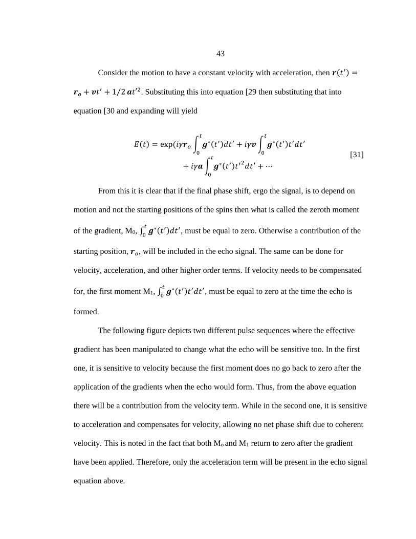
Consider the motion to have a constant velocity with acceleration, then 𝒓(𝑡′) =
𝒓𝒐 + 𝒗𝑡′ + 1 2⁄ 𝒂𝑡′2. Substituting this into equation [29 then substituting that into
equation [30 and expanding will yield
𝐸(𝑡) = exp (𝑖𝛾𝒓𝑜 ∫ 𝒈∗(𝑡′)𝑑𝑡′
𝑡
0
+ 𝑖𝛾𝒗 ∫ 𝒈∗(𝑡′)𝑡′𝑑𝑡′𝑡
0
+ 𝑖𝛾𝒂 ∫ 𝒈∗(𝑡′)𝑡′2𝑑𝑡′
𝑡
0
+ ⋯
[31]
From this it is clear that if the final phase shift, ergo the signal, is to depend on
motion and not the starting positions of the spins then what is called the zeroth moment
of the gradient, M0, ∫ 𝒈∗(𝑡′)𝑑𝑡′𝑡
0, must be equal to zero. Otherwise a contribution of the
starting position, 𝒓𝑜, will be included in the echo signal. The same can be done for
velocity, acceleration, and other higher order terms. If velocity needs to be compensated
for, the first moment M1, ∫ 𝒈∗(𝑡′)𝑡′𝑑𝑡′𝑡
0, must be equal to zero at the time the echo is
formed.
The following figure depicts two different pulse sequences where the effective
gradient has been manipulated to change what the echo will be sensitive too. In the first
one, it is sensitive to velocity because the first moment does no go back to zero after the
application of the gradients when the echo would form. Thus, from the above equation
there will be a contribution from the velocity term. While in the second one, it is sensitive
to acceleration and compensates for velocity, allowing no net phase shift due to coherent
velocity. This is noted in the fact that both Mo and M1 return to zero after the gradient
have been applied. Therefore, only the acceleration term will be present in the echo signal
equation above.

44
Figure 29: Uncompensated (top) and compensated (bottom) gradients
It is clear to see that the effective gradient can be designed for many purposes. If
one needed to compensate for constant fluid flow the sequence could be designed such
that it was sensitive to position and the first moment was zero. Also vice versa, one could
design a sequence, as above, to allow for sensitivity of velocity but negate the phase shift
due to spin starting position.
PGSE
At this point the idea of q-space imaging through the use of the pulsed gradient
spin echo (PGSE) sequence can be introduced. Much like its imaging counterpart, k,
which is tied to imaging position, q-space obtains data related to displacements which is
useful in determining things such as diffusion and velocities within a system. First, a brief
discussion of the PGSE sequence is necessary. Figure 28 is essentially a PGSE sequence,
except that the gradients in the PGSE sequence are applied quickly such that there is

45
negligible motion in the time frame in which the phase is ‘wound’. The PGSE sequence
is depicted in the following figure.
Figure 30: PGSE sequence
This sequence is a form of the previously discussed spin echo sequence. τ is the
time between the 90o and 180o RF pulses with an echo formation at 2τ. δ is the gradient
pulse time and Δ is called the mixing time, the time between the start of the two gradient
pulses. As previously discussed, the stipulation for an echo to form requires that the
zeroth moment is zero. In other words, the pair of gradient pulses must be equal and
opposite, the first ‘burning’ a phase into the spins and the second ‘unwinding’ this phase.
This results in an echo signal that is dependent on the phase related to the molecular
motion that took place during time, Δ. Stejskal and Tanner developed an idealized
equation for the normalized echo signal described by
𝐸(𝒈) = 𝑒𝑥𝑝(𝑖𝛾𝛿𝒈 ⋅ 𝒗 − 𝛾2𝑔2𝛿2𝐷(∆ − 𝛿 3⁄ )) [32]
The first contribution within the exponent describes the phase shift of a coherent
motion which displaces all the spins by the same amount, ergo steady flow, with no
signal attenuation. The second contribution represents the diffusive contribution. The
negative sign in front denotes an attenuation of the echo signal, contrary to steady flow,

46
which arises due to the incoherent diffusive motion which produces incoherent phase
shifts across the nuclear ensemble. Thus, there is a phase shift due to steady flow and a
signal attenuation due to diffusion.
Extending some concepts, if one wanted to be rid of the signal due to flow and
study only the diffusive contribution, a manipulation of the gradients could be done such
that the zeroth and first moments went to zero at the echo. Thus, the sequence would be
velocity compensated and only the attenuation due to diffusion would remain. Further,
through the use of a Stejskal-Tanner plot one could obtain the self-diffusion coefficient of
the fluid within the system of study. Clearly, this PGSE sequence is useful and has a lot
of potential for studying flow and diffusion, especially in porous media.
Q-Space and Propagators
To thoroughly understand q-space and extend the usefulness and meaning of the
PGSE sequence, the averaged propagator and its relation to the echo signal will be
discussed. First, one must take a step back and understand conditional probabilities. The
conditional probability measures the probability of an event happening given that another
event has occurred. The conditional probability for a particle to be at x1 at time t1 given
that it was initially at xo at time to is given by the joint probability of both occuring
divided by the initial probability density which is given by the following equation:
𝑃(𝑥0, 𝑡0|𝑥1, 𝑡1) =
𝑃(𝑥0, 𝑡0; 𝑥1, 𝑡1)
𝑝(𝑥0, 𝑡0) [33]
Since Brownian motion is a Markovian process, meaning that the particle position
at x1 at time t1 is not dependent on where the particle was prior to to, the probability of

47
paths can be calculated in a stepwise manner. To find the conditional probability of any
starting and finishing point, one needs to integrate over the intermediate paths. Thus
𝑝(𝑥0, 𝑡0|𝑥2, 𝑡2) = ∫ 𝑝(𝑥0, 𝑡0|𝑥1, 𝑡1) 𝑝(𝑥1, 𝑡1|𝑥2, 𝑡2)𝑑𝑥1 [34]
This can be done to find the probability of x at time t by integrating over all
starting positions. Furthermore, since our interest is in the displacement, we write the
probability density as a function of r, which is the coordinate in 3D. Thus, the three
dimensional probability density of the final position 𝒓′ at time t is
𝑝(𝒓′, 𝑡) = ∫ 𝑝(𝒓, 0) 𝑃(𝒓, 0|𝒓′, 𝑡)𝑑𝒓 [35]
Now this can be applied to the echo signal with a little thought. This equation
simply represents the probability for a spin to move during a given time. In order to find
our desired echo signal for an ensemble of spins, the phase shift of each spin is simply
weighted by the probability of that spin to move 𝒓′ at time Δ given that it was initially at
𝒓. The probability is exactly that represented in equation [35. Also, 𝑝(𝒓, 0) is exactly
representative of 𝜌(𝒓), the molecular density function, since the magnetization of the
spins at time zero is synonymous of the position of the molecular spins at time zero.
Thus, our echo signal can now be written as
𝐸(𝒈, ∆) = ∫ 𝜌(𝒓) ∫ 𝑃(𝒓, 0|𝒓′, ∆) 𝑒𝑥𝑝(𝑖𝛾𝛿𝒈 ⋅ [𝒓 − 𝒓′])𝑑𝒓′𝑑𝒓 [36]

48
To make this equation more useful and to have a Fourier relationship pair, as k-
space has with the molecular density function, a few definitions and substitutions will be
made. First, we define the reciprocal space q as
𝒒 = 𝛾𝛿𝒈 [37]
This is simply a function of the applied gradient weighted by the gyromagnetic
ratio and the gradient pulse time. We also define the displacement as being 𝑹 = 𝒓′ − 𝒓.
Finally, we introduce what is called the average propagator. This is the ensemble average
of the displacement from the origin of all possible starting positions. This essentially
yields a distributions of displacements from their initial starting positions for a certain
time. This is defined as
�̅�(𝑹, 𝑡) = ∫ 𝜌(𝒓)𝑃(𝒓, 0|𝒓 + 𝑹, 𝑡)𝑑𝒓 [38]
Now substituting those three definitions into equation [36 yields
𝐸(𝒒, ∆) = ∫ �̅�(𝑹, ∆)𝑒𝑥𝑝(𝑖𝒒 ⋅ 𝑹)𝑑𝑹 [39]
This equation is now extremely useful and provides insight into q-space and its
relationship with the echo signal. It is clearly seen that this now almost identically
resembles the Fourier relationship of equations [25 and Error! Reference source not
found. for that of k-space. So q-space acquisition allows one to obtain the average
propagator, �̅�(𝑹, ∆), where it has a Fourier relationship with the echo signal, 𝐸(𝒒, ∆), just
as k-space acquisition allows one to obtain the molecular density function. The difference
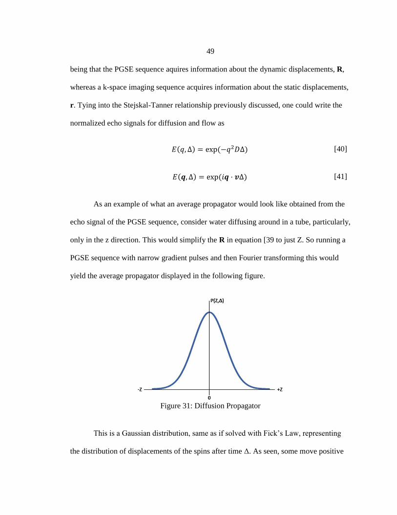
49
being that the PGSE sequence aquires information about the dynamic displacements, R,
whereas a k-space imaging sequence acquires information about the static displacements,
r. Tying into the Stejskal-Tanner relationship previously discussed, one could write the
normalized echo signals for diffusion and flow as
𝐸(𝑞, ∆) = exp (−𝑞2𝐷∆) [40]
𝐸(𝒒, ∆) = exp (𝑖𝒒 ⋅ 𝒗∆) [41]
As an example of what an average propagator would look like obtained from the
echo signal of the PGSE sequence, consider water diffusing around in a tube, particularly,
only in the z direction. This would simplify the R in equation [39 to just Z. So running a
PGSE sequence with narrow gradient pulses and then Fourier transforming this would
yield the average propagator displayed in the following figure.
Figure 31: Diffusion Propagator
This is a Gaussian distribution, same as if solved with Fick’s Law, representing
the distribution of displacements of the spins after time Δ. As seen, some move positive

50
and some move negative, there is an equal distribution of both, but most don’t move at all
or move back to the same position as they started.
This brief introduction of NMR, although seemingly long, should be enough for
one to understand the concepts presented in the following thesis. Many different pulse
sequences used to obtain various data for experiments will also be discussed in more
detail within the body of this document where the introduction will prove to be a useful
reference.

51
3. ZTE SEQUENCE OPTIMIZATION
Introduction
Imaging of rock cores and porous media can prove difficult due to the very short
relaxation times, mainly T2*, due to the increase in molecular interactions within the
small pores along with the small amount of water. Because sequences such as the spin
echo sequences require the use of a 90o and 180o pulse, as opposed to a short tip angle
used by specialized sequences, these pulses take longer to apply and by the time the RF
coil is switched to receive most of the signal, if not all, would already be gone. This leads
to the use of some specialized pulse sequences designed to image systems with ultrashort
T2*’s, such as single point imaging (SPI), single point ramped imaging with T1
enhancement (SPRITE), and zero echo time (ZTE). Information on these sequences and
more can be found in [18-20].
Therefore it is an important part of this work to explore these sequences designed
to image ultrashort T2* systems and determine what sequence would be best to use. It is
important that the sequence be able to adequately image short T2* samples and to capture
the image quickly, as some experiments will be dynamic experiments in need of a
“snapshot”. This section discusses the chosen ZTE sequence, the optimization of it, and
its advantages and disadvantages.

52
Parameter Manipulation
The ZTE sequence was chosen because it was the quickest sequence and it
provided adequate resolution. The ZTE imaging sequence [18-20] is depicted in Figure
32. Its value comes from capturing fast relaxing decays, short T2 and T2* values. This is
achieved by switching on a readout gradient before RF excitation and ramping through
gradient values acquiring k-space in a 3D radial center-out manner. By having the
gradient already switched on before excitation, there is no added down time between
acquisition and RF excitation. The only down time being the physical limit on how fast
the hardware can switch between transmit and receive, denoted by δ. Therefore, more of
the FID can be obtained at the cost of losing some initial k-space points due to the delay,
δ. Due to these missing k-space points the typical Fourier transformation for image
reconstruction does not hold. The missing k-space points and image reconstruction are
dealt with through the use of an algebraic reconstruction and 3D gridding algorithm [18].
The sequence also utilizes short tip angles, further helping to shorten TR as well as
capture the fast decay. That is, pulses that are less than 90o.
Figure 32: Three dimensional ZTE pulse sequence with hard RF pulse
In order to optimize the ZTE sequence and determine the adequate parameters, a
rubber sample was first used that had a similar short T2 relaxation time as a saturated

53
Berea rock core, i.e. on the order of 5ms. The rubber actually had a longer T2 but it made
it easier to initially image and manipulate sequence parameters by providing slightly
more signal that was uniform as opposed to dealing with saturating a rock core that had
less signal and was more heterogeneous. Parameters were therefore manipulated first
using the rubber sample then, once a better understanding of the sequence was obtained, a
saturated Berea rock core was used. Many parameters that were investigated and will be
discussed include: the bandwidth, the pulse length, the pulse power, the tip angle, the
polar under sampling, the field of view (FOV) and matrix size, the repetition time (TR),
and the reconstruction options.
In order to resolve an image, the excitation bandwidth per pixel must be greater
than the linewidth of the sample otherwise blurring will occur. Therefore, increasing the
excitation bandwidth would increase your resolution until the image was fully resolved.
However, increasing the bandwidth will lead to more missing k-space points because
faster sampling will place more points within the down time, δ, where they are not being
acquired. Therefore, there is a trade-off between bandwidth and missing k-space points
where a bandwidth greater than the optimum leads to poor image quality. It was found
that any more than 2 missing k-space points leads to poor image quality and thus a
maximum bandwidth of 200 kHz was used.
Since the ZTE sequences utilizes short tip angles, the pulse time is significantly
shorter than a 90o pulse. Since the image can’t be fully resolved, it’s important to
maintain the maximum bandwidth to achieve the best resolution possible. Bandwidth is
inversely related to the pulse length, a shorter pulse means a larger bandwidth. Therefore,
54
by maximizing our bandwidth we shorten our pulse time. Thus, if we want to change the
tip angle we must change the pulse power. So with the bandwidth maximized and the
pulse time shortened, we increase the pulse power to increase the tip angle and obtain a
FID with more signal. However, there are hardware limitations and only so much pulse
power can be achieved. Therefore, a bandwidth of 200,000 kHz resulted in a pulse time
of 6.4μs, a maximum pulse power of -3dB, a tip angle of 6.4o, and 1.8 missing points.
In order to capture the entire rock core without any artifacts, the FOV needed to
be adjusted. The FOV needed to be just big enough to capture all the rock core and any
background signal so as to not create any wrap-around artifacts but not so big that the
resolution and sequence time began to suffer. The optimum FOV in the SWB 60mm
probe was found to be around 60x90x60mm with a matrix size of 64x64x64. As latter
discussed the actual resolution was determined to be somewhere around 3mm/pixel, so a
matrix size of 643 was more than adequate. Increasing the matrix size only exponentially
increased the image reconstruction time and gradient duty cycle without providing any
additional resolution gain.
The polar under sampling was also looked at. The polar under sampling
essentially acquired less radial lines, under sampling the data and saving experiment time.
Increasing the under sampling did not show much difference. Considering its small
change in the already short sequence time, and the fact that the resolution was not fully
resolved, the polar under sampling was left at 1, sampling the entire radially space. The
repetition time (TR) was determined from the Ernst angle equation and increasing the TR
showed no improvement in the signal only lengthening the experiment time. Therefore, a

55
TR of 3.84ms was chosen as it was larger than the Ernst angle calculation but to the point
where an increase showed no further signal increase.
Image Reconstruction and Analysis
During the image reconstruction and analysis it was found that a user intensity
range needed to be specified so that the reconstructed images all had the same image
intensity intervals and were comparable. That user range was chosen to be 0 – 200,000
for the saturated Berea rock core. This allowed an accurate comparison between images
where an increase or decrease in the water saturation could be easily detected and
measured in the image intensity.
Since the saturated rock core had a small signal the background signal, from
things like the AFLAS sleeve, PEEK tube, and core holder, was significant. Two things
were done to enhance the saturated core signal and separate it from the background
signal. The first was to add Magnevist to the water to enhance the signal from the rock
core, increasing the signal intensity making it more distinguishable from the background
signal. The second was to obtain a background image with a dry rock core and use it to
subtract out the background. The background subtraction was done in Prospa where the
saturated rock matrix was subtracted from the background matrix. Figure 33 shows an
example of this subtraction. An axial slice of a fully saturated core with background
signal is subtracted from the same slice with a completely dry core where only the
background signal exists yielding only the signal from the water within the rock core.
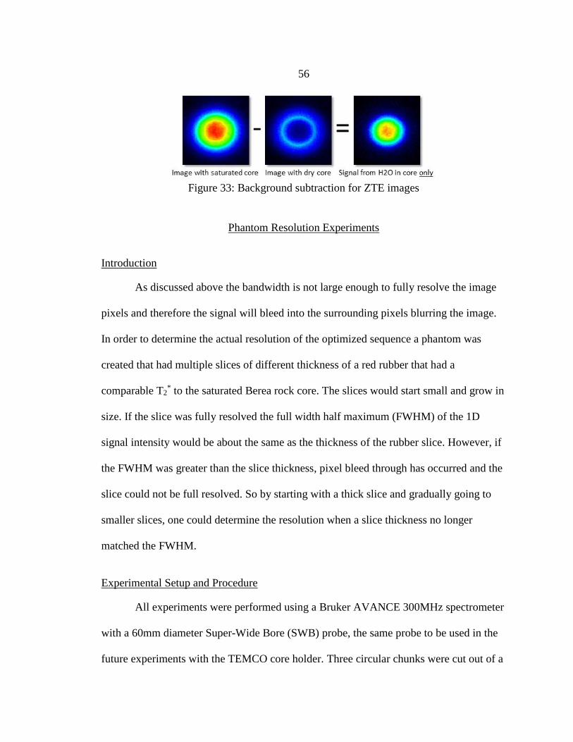
56
Figure 33: Background subtraction for ZTE images
Phantom Resolution Experiments
Introduction
As discussed above the bandwidth is not large enough to fully resolve the image
pixels and therefore the signal will bleed into the surrounding pixels blurring the image.
In order to determine the actual resolution of the optimized sequence a phantom was
created that had multiple slices of different thickness of a red rubber that had a
comparable T2* to the saturated Berea rock core. The slices would start small and grow in
size. If the slice was fully resolved the full width half maximum (FWHM) of the 1D
signal intensity would be about the same as the thickness of the rubber slice. However, if
the FWHM was greater than the slice thickness, pixel bleed through has occurred and the
slice could not be full resolved. So by starting with a thick slice and gradually going to
smaller slices, one could determine the resolution when a slice thickness no longer
matched the FWHM.
Experimental Setup and Procedure
All experiments were performed using a Bruker AVANCE 300MHz spectrometer
with a 60mm diameter Super-Wide Bore (SWB) probe, the same probe to be used in the
future experiments with the TEMCO core holder. Three circular chunks were cut out of a

57
flat sheet of rubber. One cut out of the thin sheet of rubber and two cut out of the thicker
sheet of rubber. Three thicknesses could be created: the thin one which was 1.68mm
thick, one chunk of the thick one which was 3.15mm thick, or two stacked chunks of the
thick one which was 6.3mm thick. At first it was thought to put all the different sizes
together in one image separated by 6mm of a material that yielded no signal, but as will
be shown, it proved difficult to accurately distinguish the different thickness. Therefore,
it was decided to do each thickness on its own.
A plastic tube with a Teflon platform inserted in it was used to set the rubber
sample on and placed inside the 60mm probe. First, the tube was inserted into the probe
to obtain a background image and then the rubber slice was placed on the Teflon platform
and imaged using the ZTE sequence with the optimum parameters discussed earlier. Each
rubber slice thickness was imaged and then analyzed in Prospa. Each image was
background subtracted and a sagittal section was taken from the middle of the 3D ZTE
image matrix allowing a 2D side profile to be seen of the thicknesses of the rubber
samples.
Results and Discussion
As mentioned above, it was first thought to put all the different thicknesses
together each separated by 6mm of material that yielded no signal so as to image them all
in one go. Due to bleed through as well as the very slight signal obtained from the
separating material however, this approach made it hard to accurately distinguish the
FWHM of each rubber thickness. This is depicted in Figure 34 where the left bump
represents the 6.3mm sample, the middle bump represents the 3.15mm sample, and the

58
right bump represents 1.68mm sample. The orange line represents one row of the 2D
sagittal image and the red line represents an average off all rows in the sagittal 2D image.
As seen, it is hard to distinguish a FWHM of each bump as the bumps are not sufficiently
separated.
Figure 34: Signal intensity vs. position for 3 rubber phantom samples
So it was decided to image each rubber thickness on its own. Figure 35 depicts the
1D average intensity versus position for the 6.3mm rubber phantom. At FWHM the
thickness is about 6.4mm. This is only 1.59% from the actual value, 6.3mm.
Figure 35: Signal intensity vs. position for 6.3mm phantom sample
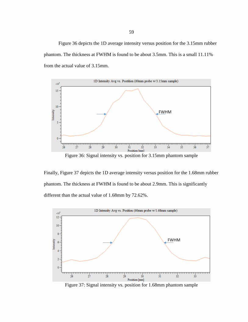
59
Figure 36 depicts the 1D average intensity versus position for the 3.15mm rubber
phantom. The thickness at FWHM is found to be about 3.5mm. This is a small 11.11%
from the actual value of 3.15mm.
Figure 36: Signal intensity vs. position for 3.15mm phantom sample
Finally, Figure 37 depicts the 1D average intensity versus position for the 1.68mm rubber
phantom. The thickness at FWHM is found to be about 2.9mm. This is significantly
different than the actual value of 1.68mm by 72.62%.
Figure 37: Signal intensity vs. position for 1.68mm phantom sample

60
Conclusions
Table 1 summarizes and compares the data for each phantom thickness. Clearly,
the 6.3mm phantom is able to be fully resolved as the percent error is only 1.59%. The
error for the 3.15mm sample yields about 11.11% which is not negligible but still small
enough to conclude that this thickness can be mostly resolved. The broadening of the
1.68mm sample to 2.90mm suggests that anything smaller than 2.90mm would not be
resolved. This in combination with the small percent difference of the 3.15mm sample
suggests that this sequence with given parameters and setup has an actual resolution of
around 3mm.
Table 1: Phantom FWHM comparison to actual thickness
60mm Probe 6.3mm Sample 3.15mm Sample 1.68mm Sample
FWHM 6.4mm 3.5mm 2.90mm
Error 1.59% 11.11% 72.62%

61
4. T1 AND T2 PRESSURE DEPENDENCE STUDY
Introduction
T1 and T2 measurements in NMR provide fundamental knowledge of the system
at hand by describing the longitudinal and transverse relaxation of the nuclear spin
ensembles, more information can be found on longitudinal and transverse relaxation
under the relaxation section in the Nuclear Magnetic Resonance Theory chapter. The
relaxation times are an indication of whether molecular motion is more solid or liquid-
like, provide a distinction between different liquids or solids, whether something is
contained in a large or small pore, whether there are surface interactions, magnetic field
susceptibilities or inhomogeneities, and many other things [16, 21]. It is therefore
important to be sure that these relaxation measurements are correct and accurate.
Otherwise, the data could be misleading or interpreted wrong. Since most of the future
experiments were going to be conducted at various high temperatures and pressures, it
was the purpose of this experiment to determine any dependence of T1 and T2 relaxation
times on pressure. It is already known that there is a dependence on temperature due to a
change in the thermal energy causing increased or decreased molecular interactions [22,
23]. Therefore, there is only a need to focus on pressure dependence in this experiment.
Experimental Setup and Procedure
Setup
All experiments were performed using a Bruker AVANCE 300MHz spectrometer
with a 60mm diameter Super-Wide Bore (SWB) probe. The flow loop is depicted in

62
Figure 38. A custom TEMCO FCH core holder designed for high-field NMR retained the
high pressure fluid. There are two regions within the core holder separated by an FEP
heat shrink sleeve. The outer region contains the confining fluid, Fluorinert, and the inner
region contains the DI H2O in a 20mm diameter PEEK tube. The confining fluid is
maintained at a higher pressure which tightly squeezes the FEP sleeve around the PEEK
tube restricting fluid from flowing around the outside. A partial cross section is shown in
Figure 38.
Figure 38: Experimental setup for pressure dependence study
Two ISCO 500D syringe pumps were used to provide the desired pressures and
flow rates. One pump was designated to maintain pressure and flow of fluids through the
bead pack while the other pump was designated to provide the confining pressure. A
TEMCO recirculation heating system provided the necessary power to heat the confining
fluid which, in turn heated the fluid going through the bead pack, which was monitored
via a thermocouple. On the outlet end of the core holder, a line ran to a beaker that caught
DI H2O as it was pumped through the system. The system could then be pressurized after

63
it was saturated with H2O, ensuring there was no air in the system, and the valve to the
beaker was closed.
Procedure
The procedure for this experiment is fairly straight forward. The system is first
setup as depicted in Figure 38. The confining fluid was pressurized to 6.89bar (100psi)
and the temperature was set to 35oC representative of the supercritical temperature to be
used in future experiments. DI H2O doped with Magnevist, used because future
experiments were going to be using Magnevist and the same conditions wanted to be
studied, was then pumped through the system at 0.689bar (10psi) until a steady flow
began to pour into the beaker. This was done to ensure that the air was completely out of
the system so as not to cause magnetic susceptibilities and compression issues. The valve
was then shut and pressure equilibrated.
Once the system temperature and pressure was equilibrated, T1 and T2
measurements were made. The pressure was then increased to 13.79bar (200psi),
maintaining the confining pressure 6.89bar (100psi) above the system pressure at all
times, and another T1 and T2 measurement were made. This continued in 13.79bar (200
psi) increments up to 124.13bar (1800psi), being careful to maintain constant
temperature. The obtained data is presented in the following section in Figure 39
andFigure 40.
Pulse Sequences
The two pulse sequences used for this experiment are the inversion recovery and
CPMG pulse sequences. They are described in the Basic Pulse Sequences and Spin

64
Manipulation section of the Nuclear Magnetic Resonance Theory chapter. The inversion
recovery sequence is used to determine the time constant T1. For a pulse power of -2dB, a
90o pulse was achieved with a pulse time of 103.5μs and 180o pulse was achieved with a
pulse time of 207.0μs. A TD=2048 and DW=50μs were used to acquire the signal with
two averages, NS=2. The list values for the inversion time points were as follows: 0.001,
0.071, 0.142, 0.214, 0.285, 0.357, 0.428, and 0.500s.
The CPMG pulse sequence is used to determine the time constant T2. The same
pulse times and power were used to achieve the 90o and 180o pulses. To acquire the FID
the following parameters were used: TD=56032, D3=400μs (Tau), DW=10μs,
D4=D6=DW, and L22=700 (number of echoes). In order to acquire a steady state signal
and increase the signal to noise, 3 dummy scans, DS=3, and 8 averages, NS=8, were
used.
Results and Discussion
The T2 values acquired from the CPMG scans are depicted in Figure 39 and the
T1 values acquired from the inversion recovery sequence are depicted in Figure 40. Both
are plotted against pressure in order to determine any trends as the pressure is increased.
The first point at 0.689bar (10psi) in Figure 39 is not comparable to the rest of the data.
An error was made in the first scan and the scan was not redone until all the other data
was collected. Upon depressurizing and redoing the 0.689bar (10psi) scan it was noticed
that the temperature had decreased by about half a degree Fahrenheit. Therefore, the
difference is attributed to the temperature and not pressure. Had the scan been conducted
at the same temperature it would be expected to fall somewhere at or slightly above the

65
T2 value at 13.79bar (200psi). However, the overall trend shows a general decrease in the
transverse relaxation, about 12ms over a large pressure range of 110.34bar (1600psi). The
change in T2 is only about 4.8% of the maximum T2 value. This decrease makes sense as
an increase in pressure compresses the substance, even though the substance is
considered incompressible it does compress albeit very minutely, causing molecular
interactions to increase, restricting the molecules rotational diffusivity and leading to a
faster relaxation [24].
Figure 39: Pressure versus T2 relaxation for doped DI H2O
Again, the first point in Figure 40 is not comparable to the rest of the data for the
same reason as mentioned above, the scan was redone after all others were conducted and
it was noticed that the temperature had decreased by about half a degree Fahrenheit. The
overall average trend in the data is a decrease in T1 with increasing pressure. The T1
decreases about 3ms over a pressure range of 110.34bar (1600psi). The change in T1 is
only about 1.0% of the maximum T1 value. However, when considering the error bars the
0.23
0.232
0.234
0.236
0.238
0.24
0.242
0.244
0.246
0.248
0.25
0 500 1000 1500 2000
T2 [
sec]
Pressure [psi]
Pressure vs. T2
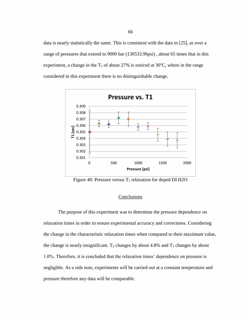
66
data is nearly statistically the same. This is consistent with the data in [25], as over a
range of pressures that extend to 9000 bar (130533.96psi) , about 65 times that in this
experiment, a change in the T1 of about 27% is noticed at 30oC, where in the range
considered in this experiment there is no distinguishable change.
Figure 40: Pressure versus T1 relaxation for doped DI H2O
Conclusions
The purpose of this experiment was to determine the pressure dependence on
relaxation times in order to ensure experimental accuracy and correctness. Considering
the change in the characteristic relaxation times when compared to their maximum value,
the change is nearly insignificant. T2 changes by about 4.8% and T1 changes by about
1.0%. Therefore, it is concluded that the relaxation times’ dependence on pressure is
negligible. As a side note, experiments will be carried out at a constant temperature and
pressure therefore any data will be comparable.
0.301
0.302
0.303
0.304
0.305
0.306
0.307
0.308
0.309
0 500 1000 1500 2000
T1 [
sec]
Pressure [psi]
Pressure vs. T1

67
5. VISCOUS FINGERING EXPERIMENTS
Introduction
Nuclear magnetic resonance (NMR) techniques have been utilized to study the
dissolution of scCO2 in water in a porous media under conditions representative of that in
a deep underground saline aquifer. CO2 is essentially immiscible in water at room
temperature conditions. By increasing to supercritical conditions, representative of a deep
underground saline aquifer, the CO2 becomes miscible in water. According to [26], the
solubility of CO2 in H2O at conditions conducted in this experiment, T = 35oC and P =
100bar (1450psi), is approximately 1.287 mol/kg or about 2.3%. This percent, although
small, should cause the NMR signal to decrease as CO2 dissolves into the H2O, restricting
the mobility of the 1H hydrogen atom and impacting the relaxation mechanisms. Thus, as
dissolution occurs the NMR signal will decrease and the dissolution of CO2 into water
can be monitored. It is the goal of this work that the interface between the CO2 and water
can be monitored moving over time from which a flux could be obtained, much like that
of the work in [12] in which numerical simulations of the convective dissolution of MEG
into water were conducted. It is therefore the focus of this experiment to extrapolate a
dissolution rate for CO2 into water and to measure the viscous fingering phenomena in
which convective dissolution occurs, further enhancing the dissolution rate, as discussed
in the introduction of this thesis. Determining the dissolution rate and studying the
viscous fingering phenomena could provide valuable information on the CO2
sequestration process, leading to enhanced storage security and process optimization.

68
Experimental Setup and Procedure
Setup
All experiments were performed using a Bruker AVANCE 300MHz spectrometer
with a 60mm diameter Super-Wide Bore (SWB) probe. The flow loop is depicted in
Figure 41. A custom TEMCO FCH core holder designed for high-field NMR retained the
high pressure fluids and housed the porous media. There are two regions within the core
holder separated by an FEP heat shrink sleeve. The outer region contains the confining
fluid, Fluorinert, and the inner region contains the 180-212 μm borosilicate glass
microspheres in a PEEK tube with Berea rock core caps. The confining fluid is
maintained at a higher pressure which tightly squeezes the FEP sleeve around the PEEK
tube restricting fluid from flowing around the outside. A partial cross section is shown in
Figure 41.
Figure 41: Experimental setup for viscous fingering experiment
Two ISCO 500D syringe pumps were used to provide the desired pressures and
flow rates. One pump was designated to maintain pressure and flow of fluids through the

69
bead pack while the other pump was designated to provide the confining pressure. A
TEMCO recirculation heating system provided the necessary power to heat the confining
fluid which, in turn heated the fluid going through the bead pack, of which was
monitored via a thermocouple. This allowed for supercritical temperatures to be reached.
On the outlet end of the core holder, a line ran to a beaker with DI H2O in it from which
water could be drawn into the bead pack to a certain level by reversing the pumps. The
system could then be pressurized after closing the valve to beaker.
Procedure
One five day experiment was conducted in which a head of scCO2 was placed on
top of DI H2O, doped with Magnevist, in a bead pack at conditions representative of a
deep saline sandstone aquifer. This experimental setup effectively replicates the CO2
sequestration scenario in which a buoyant plume of scCO2 has been trapped by a cap rock
and is on top of a denser brine layer, all within a porous sandstone, at which point
convective dissolution begins to take place, as discussed in the introduction of this thesis.
The beads were carefully placed in a 20 mm diameter by 100 mm long PEEK
tube with the bottom Berea rock cap in place and filled slightly less than full so as to
leave a small gap at the top to more clearly see the interface between the bead pack and
the head of CO2. The top Berea rock cap was then inserted. The rock caps were used not
only to hold the beads in place but, also to provide a permeable barrier that would protect
the bead pack from any sudden velocity surges that may disrupt the bead pack and
interface. After this the apparatus was setup according to Figure 41.
70
Once setup, CO2 at ambient conditions was pumped through the core at 10 ml/min
bubbling it in the beaker filled with DI H2O doped with 0.19%-vol Magnevist. The
bubbling ensured that the system was completely purged of anything but CO2 and that
when stopped no air would diffuse back into the system. After bubbling, the pumps were
reversed drawing DI H2O back into the system at 0.5 ml/min until it reaches the bead
pack and then slowed to 0.25 ml/min.
The H2O entering the bead pack was monitored by single pulse FID and 1D
spatial profiles. The 1D spatial profiles scan was used to fill the bead pack to a point
where the CO2/H2O interface was in the top 3/4s of the sensitive region in the RF coil.
This was done so that the interface could still be monitored as well as any dissolution
down into the saturated bead pack. A ZTE image was then taken assuring the location of
this interface was distinctly defined and in the appropriate position. Once the appropriate
position was obtained the pump was shut off and the valve to the beaker was closed.
The recirculation heating system was then turned on to reach the supercritical
temperature of 35oC. The pressure was slowly increased to a supercritical condition,
100bar (1450psi) while maintaining an overburden pressure 6.89bar (100psi) greater.
Once the system was equilibrated, imaging began. The system was allowed to sit for 5
days capturing ZTE and MSME images every 2 hours. The MSME images were used to
find the relaxation time T2 as well as the 2D intensity images. The MSME intensity
images were also compared against the ZTE images since this was the first big
experiment using the ZTE sequence and the MSME was an already trusted sequence.

71
Pulse Sequences
Four main pulse sequences were used to capture the necessary data: a single pulse
FID acquisition, a 1D spatial profile position-z, ZTE (zero echo time), and MSME (multi-
slice multi-echo). The single pulse sequence is the most basic pulse sequence used to
simply detect signal. A 90o RF pulse is applied to the sample and a FID is obtained. The
FID is Fourier transformed to yield a spectra in the frequency domain. Since the signal is
tuned to detect 1H nuclei, the signal is from the water protons. The more water the greater
the signal and the larger the intensity of the spectra. A 90μs RF pulse with a power level
of -3.0dB was used to achieve a 90o RF pulse.
The second sequence used is the position-z sequence. The sequence is like the one
discussed in Figure 21 of the gradients section in the Nuclear Magnetic Resonance
Theory chapter. The application of a linear magnetic field gradient in the z direction after
the application of a 90o RF pulse will result in a spectra with frequencies that are
dependent on spin position along the z axis and signal intensity that is proportional to the
number of spins associated with a certain position. Thus a cylinder full of water placed
lengthwise along the z axis would yield a spectra of a 1D profile of a rectangle when a
position-z scan is utilized. The same 90o RF pulse was used in this sequence. A
bandwidth of 50000Hz was sufficient to spectrally view the length of the sample. A FOV
along the z axis of 100 mm with 128 pixels was more than enough to capture the signal in
the entire tube. A repetition time of 5000ms was used to ensure the signal returned to
equilibrium before another pulse was applied.
The third pulse sequence used was the multi-slice multi-echo (MSME) pulse
sequence depicted in Figure 42. This sequence is used to acquire 2D slice selected images

72
with different T2 weighting. This sequence is similar to the spin-echo sequence described
in Figure 18 and Figure 24 except that a slice selective gradient is used to select a
specified slice of desired thickness in the third dimension and that an echo train of a
specified number of echoes is used to obtain multiple T2 weighted images, the number of
images dependent on the number of echoes.
Figure 42: Multi-slice multi-echo (MSME) pulse sequence
A particular use of this sequence is that, along with acquiring a 2D image, the
spin-spin relaxation time can be determined because the signal acquired at each
successive echo is attenuated by transverse relaxation. From the successive attenuated 2D
images a relaxation map like that depicted in Figure 47 can be created and the T2 value
can be found for a particular location within the image. A selective sinc3 pulse was used
with a 0.97ms pulse length at 3dB in order to achieve a 90o pulse exciting a bandwidth of
6402 Hz. 16 echoes with an echo time (TE) of 10.21 ms was used from which a
relaxation map was created from the attenuated 2D images. 1 axial slice of 0.5 mm was

73
selected with a FOV of 32x32 mm and a matrix size of 64x64 yielding a resolution of 0.5
mm/pixel.
The final pulse sequence used in this experiment was the zero echo time (ZTE).
The ZTE sequence is depicted and discussed in both Figure 25 and Figure 32. In order to
resolve the spectral information a band width of 65789 Hz was used with a 19.5 μs pulse
at 4.7 dB and a tip angle of 8o. A FOV of 32x90x32 with a matrix size of 1283 was
sufficient to capture the desired image without creating any artefacts. A repetition time
(TR) of 3.84 ms was used in order to ensure the magnetization returned to equilibrium
before the next RF pulse was applied.
Results and Discussion
Imaging of CO2 Pulse through Saturated Rock Core
Before the experiment was carried out another experiment was conducted to
evaluate if it was even possible to adequately image a saturated core, image a CO2 pulse
passing through the core, and distinguish between water and CO2 within the pores. The
idea was to image a completely dry rock core for an initial reference and background
subtraction and then saturate the rock core with H2O and bring it up to supercritical
pressure and temperatures, 75.86bar (1100psi) and 35oC. Then pump CO2 into the rock
core displacing the water in the pores. ZTE images would be taken continually to monitor
any changes in the rock core and saturation. Figure 43 depicts what the anticipated 1D
profile would look like when a pulse of CO2 passes through a saturated rock core. Green
represents a fully saturated core with the blue representing the transit of the CO2 pulse
through the rock core and red representing a drained rock core.

74
Figure 43: Expectation of 1D ZTE data for CO2 pulse
The results of this experiment are depicted in Figure 44 and Figure 45. Figure 44
displays the 1D intensity profile during the course of draining the rock core, similar to the
anticipated depiction in Figure 43. The core does drain and decrease in signal, meaning
water is being displaced out of the core. However, it does not completely remove all of
the water from the core, as noted by the remaining signal after the pulse has moved
through the rock core.
Figure 44: 1D ZTE data for CO2 front moving through rock core

75
Figure 45 shows the same water being displaced as the CO2 pulse passes through
the core but as a 2D image, both axial and sagittal. These images are achieved after a
background subtraction yielding only the signal from the water in the rock core. As the
pulse passes through the rock core the signal from the water clearly attenuates. Thus
these figures show that a rock core can be adequately imaged during saturation and
drainage and that the CO2 and water can be distinguished.
Figure 45: 2D ZTE data for CO2 front moving through rock core
Viscous Fingering Experiment
After verifying the plausibility of imaging a CO2 pulse passing through rock core,
the five day experiment was conducted in order to try and capture the CO2 dissolution in
the porous media as well as the viscous fingering phenomena which leads to convective
dissolution further enhancing mass transfer. The setup and procedure were previously
explained.

76
The intention of this experiment was to have a clear interface between the water
and scCO2, as depicted in the left ZTE image of Figure 46, in which the dissolution into
the bead pack could be clearly monitored along with the movement of the interface and
any fingering that might take place and be visible. However, as depicted in the right ZTE
image in Figure 46, there was a pressure inversion incident upon pressurizing the system.
It can be seen that the interface has moved into the bead pack but still remains fairly
distinct. Therefore, the experiment was allowed to continue with the new interface.
Figure 46: Before and after images from pressure inversion incident
As mentioned above relaxation maps were made from the MSME sequence, in
which one can spatially distinguish the spin-spin relaxation times within the bead pack.
Figure 47 depicts what these maps look like with red and yellow being the longest
relaxation times moving down to blue and black being the fastest relaxation times.
Therefore, it makes sense that in the region where CO2 has penetrated into the bead pack
and mixed with water that the relaxation times are shortened due to CO2’s molecular
interactions with the hydrogen ions in water [27]. The red and blue lines indicate the

77
position in the bead pack that Figure 49 and Figure 50 are associated with where the red
line is below the interface in the water saturated region and the blue line is above the
interface in the CO2 saturated region.
Figure 47: Relaxation map with red and blue lines indicating where T2 progressions were
taken from
Figure 48 is 34 average 1D profiles, averaging the signal across the diameter of
the tube, each created from its associated relaxation map that was made from the
chronologically taken MSME images. Therefore, this gives us an idea of how the
relaxation times associated with a longitudinal position in the bead pack changed over the
several day period. Again, the red and blue lines indicate the position in the bead pack
that Figure 49 and Figure 50 are associated with. It’s hard to distinguish any change over
the experiment duration of the relaxation times and associate that with a position in
Figure 48 because the lines are all so close together. Therefore, in order to distinguish the
difference in time Figure 49 and Figure 50 where made.

78
Figure 48: T2 1D average across length of sample for all 34 scans
Figure 49 represents the change in time of the T2 relaxation time associated with
the position as indicated by the red line in Figure 48. It can now be clearly seen that the
relaxation time is consistently decreasing at this position. It changes from ~36.8 ms to
~33.5 ms which is a decrease of about 8%. This makes sense as the dissolution of the
CO2 into the water would decrease the relaxation time [27].
Figure 49: T2 progression of scans at position 18mm versus time
Figure 50 represents the change in time of the T2 relaxation time associated with
the position as indicated by the blue line in Figure 48. Initially, it appears there is a small
decrease in the relaxation time but as time goes on the relaxation times begin to increase.

79
It changes from ~24 ms to ~26.5 ms which is an increase of about 9%. This is unexpected
but may possibly be explained by an increase of pure water (that which has no dissolved
CO2 in it) in the pores at this position. As the CO2 above dissolves into the water and
creates a denser layer of CO2 and water that then fingers down into the water saturated
bead pack, because of mass conservation, it would displace water into the upper portion
of the bead pack. This is a viable hypothesis but still remains unclear, in part because
only 2.3% of the CO2 is dissolvable in water at these conditions and the spectrometer is
unable to clearly resolve this difference.
Figure 50: T2 progression of scans at position 62mm versus time
The following two figures depict the 1D average signal intensity along the z-
direction, lengthwise along the tube as in the previous figures, for the MSME data and
the ZTE data over four days. Notice the data starts on day two as the pressure inversion
incident took place on day one, skewing the data. Therefore, it was removed to reflect the
new interface position as shown in Figure 46. In Figure 51, although slight, it appears that
in the bottom half of the tube the signal intensity decreases and in the top part of the tube
the signal intensity increases, especially in the last day. This helps to corroborate the

80
previous T2 relaxation time hypothesis in that more water is displaced into the upper
pores as the CO2 mixes with the water and plunges down.
Figure 51: 1D average signal intensity vs. position (MSME scans)
Figure 52 shows similar data as in Figure 51 except a different pulse sequence
was used to obtain the data, the ZTE sequence which is weighted for T1 relaxation rather
than T2. This data, however, does not show any significant trend over time. The lines
remain more or less on top of each other. This difference can be attributed to the pulse
sequences themselves. The MSME sequence has a higher signal to noise because more
averages are done and has a finer resolution whereas the ZTE sequence is done quickly
with minimal averages leading to a smaller signal to noise ratio. Considering the minute
changes that take place this hypothesis makes sense where the changes are barely
noticeable in the higher signal to noise ratio pulse sequence.

81
Figure 52: 1D average signal intensity vs. position (ZTE scans)
Conclusions and Future Work
Imaging the viscous fingering phenomena and quantifying the dissolution rate has
proved to be a difficult task. Things that lend itself to the difficulty include: the very
small amount of CO2 that can dissolve into the water (just 2.3% at these conditions)
leading to a small contrast in signal between the dissolved CO2/water and the water, the
inability for the imaging sequences to distinguish between the dissolved CO2/water and
just water itself because of this small percentage, the small amount of signal that can be
detected, the inhomogeneities caused by the porous media, and the unknown timeframe
and effect of viscous fingering on dissolution. This data has shown these difficulties but
also suggests dissolution was occurring over these four days and that water was possibly
being displaced by the dissolved CO2, suggested by the T2 relaxation data and the MSME
data. Therefore, it is plausible that this phenomenon can be detected and studied but
requires further testing and refinement.
In future work it would prove beneficial to take a step back and look at a more
simplified system, such as removing the porous media and just having a head of CO2 on

82
water. This would allow a higher signal to noise, a cleaner interface, and better resolution
in hopes of being able to better visualize and quantify the viscous fingering to obtain a
better understanding of the dissolution of CO2 into water. Also, one might look into
maximizing the dissolution percentage by finding the optimum conditions, therefore,
increasing the contrast between the water and the dissolved CO2/water.
Furthermore, it may prove beneficial to revisit the experiment that was conducted with
maximized conditions being careful not to disrupt the CO2/water interface, i.e., avoid a
pressure inversion. The inversion could have affected the system in unforeseen ways,
such as perturbing the whole system and causing a large amount of CO2 to dissolve
quickly, causing the system to behave differently and in a manner that doesn’t represent
the sought after phenomena.

83
6. CAPILLARY TRAPPING EXPERIMENTS
Introduction
Nuclear magnetic resonance (NMR) techniques have been utilized to
noninvasively monitor the drainage/imbibition of air, CO2, and scCO2 with DI H2O in a
Berea sandstone rock core under conditions representative of a deep underground saline
aquifer. This experiment is designed to mimic the capillary trapping mechanism
discussed in the introduction of this thesis, in which, after CO2 injection brine imbibes
back into the pores trapping CO2 ganglia via snap-off. Because of the thermophysical
properties of scCO2, analogue fluids used for simplification may not be representative of
the actual processes under geologic conditions. Thus, this study will compare the
capillary trapping of air with that of supercritical CO2. Also, subcritical CO2 will be
compared to supercritical CO2 in order to identify and analyze any distinctions in the
supercritical state from its subcritical state. Furthermore, the distribution of W fluid in the
pores will be monitored via NMR relaxometry in order to provide some insight into
which pores may trap the NW phase and to track the drainage/imbibition through the pore
structure. These experiments stemmed from the work done in [7].
Experimental Setup and Procedure
Setup
All experiments were performed using a Bruker AVANCE 300MHz spectrometer
with a 60mm diameter Super-Wide Bore (SWB) probe. The flow loop is depicted in
Figure 53. A custom TEMCO FCH core holder designed for high-field NMR housed the

84
rock core and retained the high pressure fluids. There are two regions within the core
holder separated by an FEP heat shrink sleeve. The outer region contains the confining
fluid, Fluorinert, and the inner region contains the rock core. The confining fluid is
maintained at a higher pressure which tightly squeezes the FEP sleeve around the Teflon
wrapped rock core restricting fluid from flowing around the outside of the core. A partial
cross section is shown in Figure 53.
Figure 53: Experimental setup and cross section of core holder
Two ISCO 500D syringe pumps were used to provide the desired pressures and
flow rates. One pump was designated to maintain pressure and flow of fluids through the
rock core while the other pump was designated to provide the confining pressure. A
TEMCO recirculation heating system provided the necessary power to heat the confining
fluid which, in turn heated the fluid going through the rock core, of which was monitored
via a thermocouple. This allowed for supercritical temperatures to be reached. Lastly, a
piston accumulator attached to a TharSFC back pressure regulator allowed fluid to
accumulate while maintaining the system at a constant pressure.

85
The rock cores used were a Berea Sandstone with dimensions of roughly 26mm in
diameter and 97mm long. They were both cored from a larger block of sandstone and
thus are expected to have similar properties listed in Table 2. Before heat shrinking the
FEP sleeves around the rock core, a couple layers of Teflon tape was wrapped around the
rock core to help seal the rough rock exterior against the FEP helping to prevent flow
around the core.
Table 2: Berea Sandstone Properties
Sandstone Dunham
Classification
Porosity Permeability
Berea quartz arenite ~15% ~150mD
Procedure
Three separate drainage and imbibition experiments were performed on two
different rock cores. Each experiment used either air, CO2, or scCO2 as the non-wetting
(NW) fluid and DI H2O, doped with 0.4%-vol Magnevist to enhance the signal, as the
wetting (W) fluid. The drainage and imbibition experiment was then repeated for each
rock core, for each NW fluid yielding a total of 6 experiments for each rock core. This
duplication is done to help verify the results for each rock core as well as show any
variations/similarities between rock cores. The results for each rock core are expected to
be similar because these cores were taken from the same block of sandstone and because
Berea Sandstone is fairly homogenous.
The experimental process is exactly the same for every experiment except for the
difference in the chosen NW fluid. Every experiment was conducted at 75.86bar

86
(1100psi) and 70oF for air/CO2 or 95 oF in order for CO2 to reach a supercritical state,
scCO2. The experimental steps were as follows:
1. The core is wrapped with Teflon tape, heat shrunk in the FEP sleeve, and placed
into the core holder which is then placed into the probe in the spectrometer and
fluid lines attached. A ZTE image is taken with the core completely dry to obtain
a background image that is later used for background signal subtraction.
2. DI H2O doped with Magnevist is then pumped in saturating the core. It is then
slowly pressurized to the desired 75.86bar (1100psi) at the same time maintaining
the confining pressure 17.24bar (250psi) above the core pressure. The saturation
is monitored via the FID produced by a modified single pulse sequence allowing
for detection of very short T2’s. Once the FID area, representative of the amount
of H2O in the sample, has stabilized, this is assumed to be maximum saturation
and a ZTE image and 1D T2 are taken for full saturation.
3. Once pressure has equilibrated at 75.86bar (1100psi), pump A is isolated and the
fluid is switched to the desired NW fluid (air, CO2, or scCO2 if the heating
recirculation system is turned on) and pumped into the core, simulating drainage,
at 0.5ml/min corresponding to very low Ca numbers (≈ 2.72E-08, 2.39E-07, or
8.09E-08). It is pumped in for about 15 minutes until it appears the FID area has
reached a fairly stable regime. Several ZTE images and 1D T2’s are taken during
the drainage process with the final one taken at maximum drainage when the FID
stabilizes.

87
4. Pump A is now isolated and the fluid is switched to DI H2O doped with
Magnevist for the imbibition phase. The water is pumped in at 0.5ml/min
corresponding to low Ca numbers (≈ 1.38E-06, 3.21E-06, or 3.50E-06). It is
pumped in for about 10 minutes until the FID area has stabilized and reached an
equilibrium like state. A ZTE image and 1D T2 are taken after stabilization and
represent the final imbibition saturation, the residual saturation.
5. The core is then removed, oven-dried, and placed in a vacuum in order to ensure
all water and NW phase have been removed so the beginning conditions of the
rock core remain the same for every experiment.
Pulse Sequences
Two main pulse sequences were used in order to capture the necessary data: zero
echo time (ZTE) and CPMG. The CPMG pulse sequence is a basic spin echo pulse
sequence that consists of a 90o RF pulse followed by sequential 180o pulses that induce
spin echoes. These spin echoes create an exponential decay envelope. Since the envelope
of decays is determined only by T2 relaxation, the time constant T2 can be determined.
For samples where multiple T2’s may be present, such as in porous media with different
pore sizes, a multi-exponential decay envelope is obtained. An inverse Laplace transform
(ILT) algorithm is then used to create a 1D distribution of T2 values representative of the
distributions within the sample. In order to pick up the extremely short T2’s in the rock
core, values of the pulse sequence were pushed to the hardware limits. A 90μs RF pulse
was obtained at max power with 500 echoes covering the short T2 decay with an echo
time of 140μs.

88
The ZTE imaging sequence [18-20] is depicted and discussed in Figure 32. Its
value comes from capturing fast relaxing decays, short T2 values. Since there is a trade-
off between bandwidth and missing k-space points, where a bandwidth greater than the
optimum leads to poor image quality, it was found that any more than 2 missing k-space
points leads to poor image quality and thus a maximum bandwidth of 200kHz was used.
A tip angle of 6.4o at maximum power yields a pulse time of 6.4μs. A TR of 3.84ms was
used and is greater than the needed TR, calculated from the Ernst angle equation, thus
giving adequate time for the longitudinal magnetization to recover. A FOV of 60mm x
90mm x 60mm with 643 pixels is adequate to image the rock core without creating any
wrap-around artifacts. The suggested resolution of 0.938mm/pixel x 1.41mm/pixel x
0.938mm/pixel is inaccurate because the maximum bandwidth used is much less than the
required bandwidth to achieve this resolution. Through the use of multiple phantoms of
varying size it was estimated that the minimum resolution that can be resolved is about
3mm/pixel. The total scan time was approximately 58 seconds providing quick snapshots
of the real time process.
Results and Discussion
AFLAS and FEP Sleeves
In preliminary experimental runs, two different confining sleeves were used and
tested. The sleeve needed to seal against the rock core forcing flow to go through the rock
core and not around, it needed to be inert against the supercritical CO2, and it needed to
have minimal or no signal contribution. During testing several significant differences

89
between the AFLAS and FEP sleeves were noticed. The first significant difference is
displayed in Figure 54.
Figure 54: T2 distribution comparisons between AFLAS and FEP
Figure 54 displays the T2 distributions for four different runs during full
saturation, three of which are a Teflon wrapped core in a FEP heat shrink sleeve and one
of which an AFLAS sleeve is used. Although the distributions cover about the same
range of values, it is noticed that the AFLAS run has distinctly one smooth population
whereas the FEP runs have what appears to be two populations. Because the FEP sleeves
have no signal and the AFLAS sleeves do, verified through imaging of just the sleeves, it
make sense that the signal from the AFLAS sleeve would contribute to the overall T2
distribution therefore altering it from the FEP data, which is believed to be the signal
from just the water in the core due to the fact that there is no signal from the FEP. In
conjunction with the hypothesis that the AFLAS sleeve also may have significant surface

90
relaxation effects on the water, it makes sense that the use of the AFLAS sleeve alters the
actual T2 distribution and is therefore not representative of the sample itself.
Another downfall of the AFLAS sleeve is its reaction to the carbonic acid created
as a results of introducing CO2 to water during the drainage phase. This can be seen in
Figure 55 where the AFLAS sleeve signal contribution becomes more intense as time
goes on. This increase in the NMR signal indicates an increase in the molecular mobility
of the sleeve which may be due to a solubilization of the material from its reaction to the
created carbonic acid.
Figure 55: ZTE images of AFLAS time evolution reaction to CO2
Figure 56 shows two pictures of the aftermath of the sleeve reaction. The choice
to go with a Teflon wrapped core and an FEP sleeve was made because of the significant
signal contribution from the AFLAS and its severe reaction to the introduction of CO2.
The FEP sleeve is ideal because it doesn’t react with the CO2, it has no signal
contribution, and when the core is wrapped with Teflon the flow will be restricted from
going around the core.

91
Figure 56: AFLAS sleeve failure
ZTE Data
Drainage and imbibition experiments were performed under conditions
representing a CO2 sequestration scenario with a specific interest into the residually
trapped amount of NW fluid due to capillary forces. The capillary trapping efficiency was
investigated for three different NW fluids (air, CO2, and scCO2) using two different
Berea Sandstone rock cores. The wetting fluid being DI H20. Three dimensional images
were taken via the ZTE pulse sequence and the data was analyzed in Prospa. At the
beginning of each experiment a ZTE image was taken of the dry rock core to provide a
background image of the signal that could then be subtracted from the saturated images,
via matrix operations within Prospa, providing only signal from the water within the
pores.
A ZTE image was taken at full saturation, several during the drainage process,
and one more at the end of the imbibition process. The three most important images, for
calculating the fraction of residually trapped NW fluid and capillary trapping efficiency,

92
are the full saturation image, the last drainage image, and the final imbibition image. The
3D ZTE images were broke down into a 1D average profile across the length of the core,
the z-direction. This was done by selecting the center, sagittal 2D plane of the rock core
and averaging each line in the transverse plane making a 1D sagittal profile. These
profiles are depicted in Figure 57Figure 58Figure 59 for air, CO2, and scCO2 as the NW
phase. These figures represent the most recent experiments on rock core #3 (as a note, the
experiments refer to rock core #2 and #3 and not #1 because #1 was used to work out the
bugs). The other 9 profiles for the other experiments were left out due to their similarities
to these three and are thus represented in the data tables and attached in the appendices.
Figure 57: 1D profiles indicating W phase along rock core length (air/H2O)

93
Figure 58: 1D profiles indicating W phase along rock core length (CO2/ H2O)
Figure 59: 1D profiles indicating W phase along rock core length (scCO2/ H2O)
The red line indicates maximum saturation, the green lines indicate the saturation
during drainage in chronological steps as signal decreases, and the blue line indicates the
maximum saturation reached after imbibition. All lines represent the signal associated
with the wetting phase saturation, so in order to obtain the NW phase saturation fraction
the data is normalized and the difference from maximum saturation, being 1, is thus the
fraction of NW phase within the pores. This is, assuming that all the pores are initially
full of the wetting phase.

94
Examining each of the 1D profiles for air, CO2, and scCO2 is it clear to see that
they have very similar profiles and intensities. In-flow artifacts appear in the 3D ZTE
images and are pronounced in the 1D profiles as signal spikes in the intensity, the several
signal spikes are on the right side around 72-80 mm. RF roll-off occurs at both the left
and right ends of the FOV and thus the signal intensity decreases. Due to these artifacts,
the NW phase fractions are calculated based on the average signal intensity in the most
linear region of the profiles, that being from 28-54mm.
The NW phase fraction data for each 1D profile of every experiment is depicted
in Table 3and Table 4. The data represents the fraction of NW phase within the pores.
The key NW phase fractions are those highlighted in yellow. There are several noticeable
trends. The first is that both CO2 and scCO2 tend to drain the core more than air in the
same period of time, indicated in the drainage-4 line in Table 3 and Table 4. For core #2,
CO2 drains the core, on average, about 9.5% more than air, and scCO2 drains the core
about 7.5% more than air. For core #3, CO2 drains the core, on average, about 5.5% more
than air, and scCO2 drains the core about 6.5% more than air. After imbibition, CO2 is
noticed to have the largest amount of trapped NW phase when compared to air and
scCO2, indicated in the imbibition final line in Table 3 and Table 4. On average, about
6.5% more CO2 is trapped than air and about 8.0% more CO2 is trapped than scCO2 for
core #2. For core #3, on average, about 3.0% more CO2 is trapped than air and about
5.0% more CO2 is trapped than scCO2.

95
Table 3: Non-wetting phase fraction in Berea rock core #2
Scan (Non-
Wetting
Phase)
Normalized Average 1D Intensity from 28-54mm
Run (Sleeve
Material)
Air
(AFLAS)
Air
(FEP)
CO2
(FEP)
CO2
(FEP)
scCO2
(FEP)
scCO2
(FEP)
Fully Saturated 0 0 0 0 0 0
Drainage-1 0.00 0.01 0.02 0.02 0.40 0.30
Drainage-2 0.30 0.22 0.36 0.43 0.44 0.40
Drainage-3 0.35 ----- 0.47 0.48 0.49 0.43
Drainage-4
(SInitial)
0.41 0.42 0.51 0.51 0.51 0.47
Imbibition
Final (SResidual)
0.28 0.32 0.36 0.37 0.27 0.30
Trapping
Efficiency
(SResidual/SInitial)
0.68 0.76 0.71 0.73 0.53 0.64
Table 4: Non-wetting phase fraction in Berea rock core #3
Scan (Non-
Wetting
Phase)
Normalized Average 1D Intensity from 28-54mm
Run (Sleeve
Material)
Air
(FEP)
Air
(FEP)
CO2
(FEP)
CO2
(FEP)
scCO2
(FEP)
scCO2
(FEP)
Fully Saturated 0 0 0 0 0 0
Drainage-1 0.10 0.03 0.01 0.04 0.19 0.18
Drainage-2 0.35 0.36 0.34 0.39 0.42 0.40
Drainage-3 0.38 0.40 0.41 0.44 0.44 0.42
Drainage-4
(SInitial)
0.40 0.44 0.47 0.48 0.49 0.48
Imbibition
Final (SResidual)
0.30 0.32 0.33 0.35 0.29 0.29
Trapping
Efficiency
(SResidual/SInitial)
0.75 0.73 0.70 0.73 0.59 0.60
The last noticeable trend appears in the trapping efficiency. The trapping
efficiency is just the ratio of the residually trapped amount of NW phase to the maximum
amount of NW phase that was in the core after drainage. For core #2, the average

96
trapping efficiency for air and CO2 are the same whereas scCO2 differs from air by about
13.5% and from CO2 by about 13.5%. For core #3, the average trapping efficiency for air
and CO2 only differ by about 2.5% where as scCO2 differs from air by about 14.5% and
from CO2 by about 12.0%. This is a significant amount of variation of the trapping
efficiency of scCO2 from both air and CO2. The scCO2 trapping efficiency is found to be
about 10% less than values reported on in [6] for similar sandstones of Bentheimer and
Doddington. However the trapping efficiency for air and CO2 are on par with their
reported results. This is more suggestive of results obtained in [8, 9] where scCO2 has a
lower residual saturation than for an analogue strongly water-wet system, air and water.
Furthermore, as the contact angle increases, snap-off is less favored and gives way to a
more piston-like advance. With the suppression of snap-off there is decrease in residual
saturation [8, 9, 28]. Therefore, this suggests that scCO2/water is not strongly water-wet
leading to larger contact angles, a decrease in snap-off, and therefore a lower residual
saturation.
It appears that CO2 and air have very similar trapping efficiencies but differ in
both the amount of NW phase drained and the residual amount of NW phase trapped.
ScCO2 has similarities to air in the amount of residual NW phase trapped and similarities
to CO2 in the maximum amount of NW phase drained but it has significant differences in
the trapping efficiency when compared to both air and CO2. From this three trends are
observed. The first is that CO2 and scCO2 drain the core to a higher maximum value than
does air. The second is that CO2 traps the largest residual amount of NW phase when
compared to air and scCO2. Finally, air and CO2 have similar trapping efficiencies
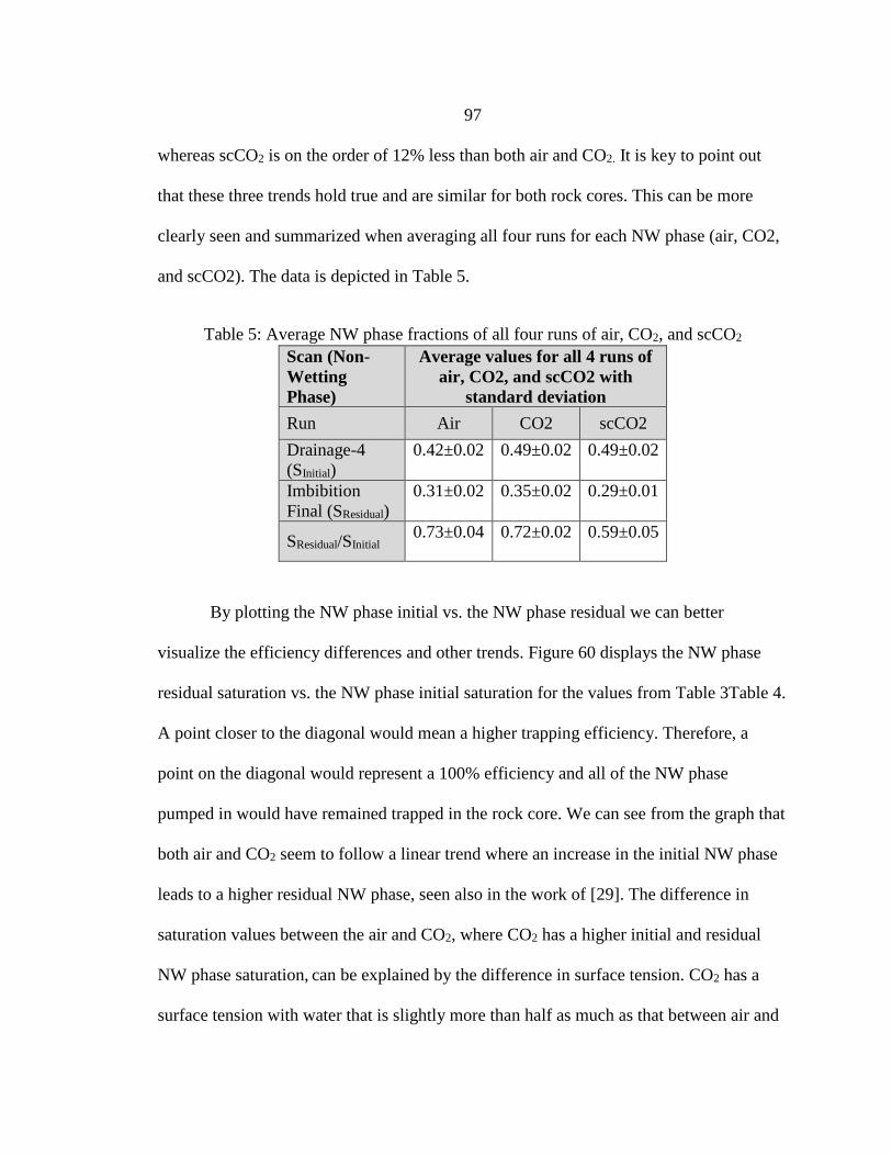
97
whereas scCO2 is on the order of 12% less than both air and CO2. It is key to point out
that these three trends hold true and are similar for both rock cores. This can be more
clearly seen and summarized when averaging all four runs for each NW phase (air, CO2,
and scCO2). The data is depicted in Table 5.
Table 5: Average NW phase fractions of all four runs of air, CO2, and scCO2
Scan (Non-
Wetting
Phase)
Average values for all 4 runs of
air, CO2, and scCO2 with
standard deviation
Run Air CO2 scCO2
Drainage-4
(SInitial)
0.42±0.02 0.49±0.02 0.49±0.02
Imbibition
Final (SResidual)
0.31±0.02 0.35±0.02 0.29±0.01
SResidual/SInitial 0.73±0.04 0.72±0.02 0.59±0.05
By plotting the NW phase initial vs. the NW phase residual we can better
visualize the efficiency differences and other trends. Figure 60 displays the NW phase
residual saturation vs. the NW phase initial saturation for the values from Table 3Table 4.
A point closer to the diagonal would mean a higher trapping efficiency. Therefore, a
point on the diagonal would represent a 100% efficiency and all of the NW phase
pumped in would have remained trapped in the rock core. We can see from the graph that
both air and CO2 seem to follow a linear trend where an increase in the initial NW phase
leads to a higher residual NW phase, seen also in the work of [29]. The difference in
saturation values between the air and CO2, where CO2 has a higher initial and residual
NW phase saturation, can be explained by the difference in surface tension. CO2 has a
surface tension with water that is slightly more than half as much as that between air and

98
water. A lower surface tension will lead to lower overall capillary entrance pressures
within the pores of the rock. With a lower capillary entrance pressure than that for the
air/water system but with the same flow rate, the viscous forces will therefore be stronger
in comparison to the capillary forces. Thus, CO2 will invade more pores leading to a
higher initial NW phase saturation.
ScCO2 does not fall on this same linear line that air and CO2 seem to fall on. It is
farther away from the diagonal than air and CO2, thus having a lower trapping efficiency.
It does fall on the same initial NW phase interval as CO2, due to the similar surface
tension values, but with a lower residual NW phase. This lower residual NW phase
saturation can be explained by the hypothesized increase in the contact angle leading to
less favorable snap-off conditions and thus a lower residual NW phase saturation, as
previously mentioned. Furthermore, by fitting a line through the air and CO2 data and
forcing it to go through zero, in order for the trend in saturation to have basis in reality,
one would obtain a slope of the linear fit that is near exactly the average trapping
efficiency value in Table 5. The same holds true if a linear trend is fit through the scCO2
data. This further validates the linear trend in the trapping efficiency and more clearly
distinguishes the difference of scCO2 from that of air and CO2.

99
Figure 60: NW phase initial vs. NW phase residual
T2 Distribution Data
The transverse relaxation times where obtained using the CPMG pulse sequence.
This yielded a multi-exponential decay curve which was inverse Laplace transformed
using MATLAB in order to obtain a distribution of T2 values. The T2 distributions were
obtained at the same significant stages as the ZTE images. The T2 values are associated
with different pore sizes within the rock core [30]. The increased interactions of nuclei in
small pores as well as surface relaxation effects contribute to the decrease of T2 as pore
sizes become smaller. Therefore, larger T2 values (slower relaxation) are attributed to
larger pores and smaller T2 values (faster relaxation) are attributed to smaller pores. This
is illustrated in Figure 61 where there are essentially two distributions that can be split
into smaller and larger pores.

100
Figure 61: Illustration for defining larger and smaller pores associated with transverse
relaxation times
In all T2 distributions there appear to be two main distributions which we
associate to larger and smaller pore sizes [10, 31, 32]. The third distribution on the far left
continues off to infinity. It cannot be resolved because the pulse time and echo time could
not be shortened any further due to hardware limitations, therefore missing most of the
extremely fast relaxing signal. These extremely fast relaxing spins are associated with
micro-porosity clay-bound water [10, 31]. Because this water is immobile and of
minimal contribution to the overall signal, it is ignored when discussing the drainage and
imbibition within the pore structure.
Figure 62, Figure 63, and Figure 64 depict the T2 distributions during full
saturation, drainage, and imbibition of air, CO2, and scCO2 as the NW phase with the
wetting phase being DI H2O doped with Magnevist. These figures are the results from
the three most recent experiments of air, CO2, and scCO2 on rock core #3. They are

101
representative of the rest of the T2 distributions and have a similar trend which is why the
others have been left out. They can be found in the attached appendices for reference.
Figure 62: T2 distribution evolution for drainage/imbibition of air/water at 75.86bar and
ambient temperature
Figure 63: T2 distribution evolution for drainage/imbibition of CO2/water at 75.86bar and
ambient temperature

102
Figure 64: T2 distribution evolution for drainage/imbibition of scCO2/water at 75.86bar
and 35oC
All distributions exhibit the same trends. They have values between about 10-3
and 10-1s with intensities that are relatively similar. There appear to be two populations
that are centered on about 10-2.3 and 10-1.6s. The left population is associated with the
micro-porosity and the right population is associated with the macro-porosity. The key
thing to take from these distributions is that during imbibition it appears only the micro-
porosity is filling with water where the macro-porosity remains the same. This is seen in
the fact that there is no change from the final drainage line (green) to the imbibition line
(blue) within the macro-porosity whereas there is an increase in saturation in the micro-
porosity. It can therefore be deduced that the NW phase is preferentially trapped in the
larger pores due to the lack of signal in the macro-porosity during imbibition. This could
be due to the fact that the pore-throat aspect ratio, the ratio of the pore body radius to the

103
throat radius, is greater in the macro-porosity giving rise to more favorable snap-off
conditions [7, 8, 33, 34].
5mm Core T2 Distribution Data
In order to fully resolve the extremely fast relaxing spins and add more validity to
the macro and micro-porosity regions of the T2 distributions, a saturated 5mm core was
placed in a 5mm probe where shorter pulse times could be achieved and the signal from
the short T2’s could be captured. To capture this, a 10μs RF pulse was used with 6000
echoes and an echo time of 16μs.
Figure 65 shows the fully resolved T2 distribution in red compared to the T2
distributions captured in the SWB probe where the very fast relaxing spins cannot be
captured. As expected, the distribution was fully resolved and three populations are
present. In [31] they discuss three different regions in the porous sandstone structure that
can be associated with different relaxation times. The first is micro-porosity clay-bound
water. It is associated with the far left population because the immobility and very small
pore sizes result in the smallest T2 values. The second is called the meso-porosity
capillary-bound water. It is discussed as the micro-porosity in the above content because
the clay-bound water is not expected to move and therefor the distribution is assumed not
to change. This is associated with the middle population because the pore size is slightly
greater and surface relaxation effects aren’t as strong. The third is called the macro-
porosity free water. It is associated with the right most population because the pore size is
yet larger and surface relaxation effects are yet less strong.

104
As expected the left population that goes off to infinity in the SWB T2 distribution
is resolved into a single population. Because this population is associated with the clay-
bound water it is expected to be immobile and the population is not expected to change
during drainage and imbibition. Therefore, it further justifies the assumption in the
previous material where the far left population that can’t be resolved, can thus be ignored
as it does not contribute to the desired data and the right two populations are indeed
associated with the smaller pore, capillary-bound water and the larger pore, freer water.
As a drainage/imbibition experiment cannot be performed on the 5mm core this
assumption and justification is the best that can be accomplished.
Figure 65: T2 distribution comparison of 5mm and 27mm cores
The fact that the 5mm core populations do not line up with the SWB populations
can be attributed to the ILT. Because a smaller core was used in a smaller probe where
different pulse times used and a more complete data set was acquired the ILT data will be

105
different. It is expected that if the SWB data could be fully captured and resolved that it
would shift left and resemble the fully resolved 5mm core distribution data.
Conclusions and Future Work
This work demonstrates the usefulness of NMR in determining the residually
trapped NW phase as well as providing insight into the pores in which the NW phase is
preferentially trapped. The results provide for a comparison between the different NW
phases used as well as characterizing the capillary trapping of each NW phase. Several
trends are apparent when comparing each NW phase:
1. scCO2 and CO2 drain the core to a higher NW phase fraction than air
2. CO2 traps the largest residual amount of NW phase
3. scCO2 traps the lowest residual amount of NW phase and has a trapping
efficiency about 13% less than CO2 and air, further justified by Figure 60
4. air and CO2 seem to follow a linear trend where an increase in the initial NW
phase leads to an increase in the residual NW phase where they hover around a
trapping efficiency of about 72%
Because scCO2 has a lower residual NW phase saturation than air and CO2, it can
be concluded that scCO2/water is not as strongly water-wet. This means scCO2/water
have larger contact angles which lead to a suppression of snap-off and therefore a lower
residual NW phase saturation [8, 9, 28]. This data suggests that air is not a good proxy for
scCO2 and that CO2, when in its supercritical state, behaves differently and leads to a
reduction in capillary trapping.

106
Lastly, the T2 distribution data shows that the NW phase, regardless of whether its
air, CO2, or scCO2, is preferentially trapped in the larger pores. This result is supported
by the findings of [33, 34]. This is most likely due to the fact that snap-off conditions are
more favorable in the macro-porosity. Meaning, the aspect ratio is greater and a piston-
like flow does not occur.
Future Work
This work has proved the usefulness of NMR in characterizing the trapping of
fluids in porous media. There is a multitude of things that can be pursued to advance this
work. There are some planned future experiments in which low field NMR spectroscopy
is utilized. In a low field spectrometer the image resolution may be lower, however
susceptibility impacts on T2 relaxation will be minimized and therefore all water in the
sample will be able to be analyzed with the T2 method, and all experiments will be able to
be carried out on a wider variety of geological materials. This work presents a
preliminary example of how NMR might inform us about the location of the imbibed or
trapped fluid.
Another thing that may prove useful to pursue is to use different flow rates, Ca
numbers, and study how the trapping efficiency varies as well as the location of the
trapped fluid. This would provide insight into the optimum situations for maximizing the
amount of trapped fluid. It would be expected that, to a point, the trapping efficiency
would increase with lower Ca numbers and subsequently, decrease with higher Ca
numbers. Hypothesized from the role between viscous and capillary forces where an

107
increase in the flow rate would increase the viscous forces and subsequently, overcome
the capillary forces that trap the NW fluid.
Another insightful study would be to test fluids with lower and higher surface
tension values to see if, as hypothesized between air and CO2, they would fall on higher
and lower NW phase initial saturations where the efficiency value could give one an idea
of the contact angle by comparison. As discussed, a lower surface tension will lead to
lower overall capillary entrance pressures within the pores of the rock. Thus, the viscous
forces will therefore be stronger in comparison to the capillary forces for a given flow
rate, and the NW fluid will invade more pores leading to a higher initial NW phase
saturation. Again, this knowledge would prove beneficial in optimizing the amount of
NW fluid to be trapped.
Furthermore, this research could be applied to different porous media to study the
best geologic scenarios for sequestering CO2. It would also provide further insight into
how and where the NW fluid is trapped and to any limits and idealities of trapping. This
work could further be extended to enhanced oil recovery (EOR) to study and optimize the
process.

108
7. TWO PHASE FLOW EXPERIMENT
Introduction
Two-phase flow in porous media is an important part of many industries and
science, such as enhanced oil recovery, fluidized beds, and water-cooled nuclear reactors
to name a few. However, because two phase flow can be unpredictable, there is a lot that
isn’t understood. Therefore, understanding the fluid behavior and mechanics of
immiscible two phase flow could prove valuable to providing more efficient designs and
to ensure the system behaves and reacts as expected. Thus, being able to determine the
flow structure and understanding the fluid mechanisms from a relationship between the
capillary number and the pressure gradient could prove valuable.
Previous numerical simulations and calculations by Sinha, [35], have studied the
nonlinearity of the pressure gradient versus capillary number in an immiscible two-phase
flow through a porous media. They demonstrate that in the region where the capillary
forces are comparable to the viscous forces, the fluids behave similar to a Bingham fluid.
That being, there is effectively a yield threshold to overcome before the fluids begin to
displace. This is essentially the threshold pressure that must be overcome. Furthermore,
they developed a generalized Darcy equation that described this relationship where the
equation was given by (∆P – ∆Pc) ∼ Caβ, where ∆P is the pressure difference across the
porous media, ∆Pc is the threshold pressure previously mentioned, Ca is the capillary
number, and β is the scaling factor. They found that β = ½ for low capillary numbers and
β = 1 for high capillary numbers.
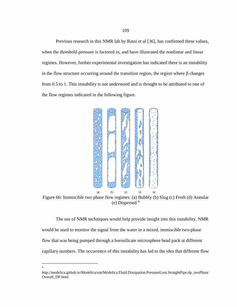
109
Previous research in this NMR lab by Rassi et al [36], has confirmed these values,
when the threshold pressure is factored in, and have illustrated the nonlinear and linear
regimes. However, further experimental investigation has indicated there is an instability
in the flow structure occurring around the transition region, the region where β changes
from 0.5 to 1. This instability is not understood and is thought to be attributed to one of
the flow regimes indicated in the following figure.
Figure 66: Immiscible two phase flow regimes: (a) Bubbly (b) Slug (c) Froth (d) Annular
(e) Dispersed 4
The use of NMR techniques would help provide insight into this instability. NMR
would be used to monitor the signal from the water in a mixed, immiscible two-phase
flow that was being pumped through a borosilicate microsphere bead pack at different
capillary numbers. The occurrence of this instability has led to the idea that different flow
4
http://modelica.github.io/Modelica/om/Modelica.Fluid.Dissipation.PressureLoss.StraightPipe.dp_twoPhase
Overall_DP.html

110
regimes could correspond to different capillary number/pressure drop relationships and
have an effect on the exponent value β. The NMR data would provide a visualization and
quantitative data to help qualify different flow patterns and would be used to help
characterize these flow patterns and their relationship to capillary number, pressure drop,
and β value. The following work presented was a collaboration of efforts from several
students within the MRM lab at Montana State University; Matt Dancyk, Andrew
Bender, Kevin Izard, and Linn Thrane.
Experimental Setup and Procedure
Setup
The previous experiments that were conducted, where the NMR spectrometer
wasn’t used, were nearly the same as the experiments conducted in this thesis where the
only difference was the length of line between the two pressure transducer ends. This was
because more tubing was needed to hook the bead pack up inside the magnet. This would
yield an overall higher pressure difference but the same trends should follow.
The setup is depicted in Figure 67 where the wetting and non-wetting fluids are
mixed and pumped through the bead pack in the NMR spectrometer and out into a beaker
at atmospheric conditions. The check valves are in place to ensure that one fluid does not
enter the other fluid’s line. The filter helped mix the two fluids and also keep any small
particles from entering the bead pack and blocking flow. The flow rate of each fluid was
controlled by an ISCO 500D syringe pump. The pressure difference was measured by a
single differential Omega pressure transducer with a 0-1.03 bar (0-15 psi) range hooked
to a DAQ where data was controlled by a LabVIEW program. All NMR experiments

111
were performed using a Bruker AVANCE 300MHz spectrometer with a 20 mm diameter
Wide Bore (WB) probe.
Figure 67: Two phase flow setup diagram
Procedure
The procedure is quite simple. One pump was filled with the wetting fluid (water)
and the other pump was filled with the nonwetting fluid (air). A flow rate was set on each
pump and allowed to run until both pumps were empty. While the pumps were running
the pressure transducer would acquire the differential pressure drop and the NMR
spectrometer would utilize pulse sequences to obtain data. The flow rate could be
changed in order to obtain different Ca numbers that would correspond to the nonlinear
or linear regions, β = 0.5 or 1 (the focus of this thesis is around the transition region,
where β changes from 0.5 to 1, and in the nonlinear region).
Pulse Sequences
The NMR spectrometer utilized the single pulse and 1D imaging sequences
discussed in the pulse sequences section of the viscous fingering experiments chapter but
112
with some modifications. The single pulse free induction decay (FID) is the most basic
pulse sequence used to simply detect signal. A single NMR radio frequency, RF, pulse
excites the protons in the liquid H2O in the sample and the free induction decay (FID)
that is acquired immediately afterwards can be directly correlated to the total water
content within the sample. A 0.1 ms RF pulse with a power level of 15.2 dB was used to
achieve a 90o RF pulse with a bandwidth of 12800 Hz. 1024 points of the FID were
obtained. It was set up so that 35 sequential scans would be obtained with a 10 second
delay between each, yielding a total acquisition time of about 5.8 minutes. This resulted
in a matrix of data that was 1024 x 35 where there was 35 sequential FIDs.
The MSME sequence is depicted in Figure 42. For this sequence however, the
phase gradients were eliminated and no echo train was used therefore becoming a 1D
imaging sequence thus yielding a single 1D profile selected along the z-axis, the
longitudinal length of the bead pack. A BP32 pulse with a 0.1 ms pulse length at 15.2 dB
was used to achieve a 90o excitation pulse with a bandwidth of 12800 Hz. The 180o
refocusing pulse thus excited a bandwidth of 8000 Hz at 9.2 dB. The 1D profile was
obtained from a 30 mm length along the z-axis averaged over a 50 mm wide slice with
128 matrix points along the length of the acquired profile. A repetition time of 3 seconds
was used in order to allow the magnetization to return to equilibrium. It was set up such
that 100 sequential scans would be obtained with a 10 second delay between each,
yielding a total acquisition time of about 16.7 minutes. This resulted in a matrix of data
that was 128 x 100 where there was 100 sequential 1D profiles.

113
Results and Discussion
Figure 68 displays the obtained pressure drop curve for a given flow rate. The
steady state (SS) region depicted is the section is where the pressure drop was averaged
and a single value was obtained. The threshold pressure was determined to be the value
the pressure curve returned to in the long time regime. The pressure drop was subtracted
from the threshold pressure, as in the equation discussed in the introduction, and plotted
on a log scale for a given flow rate. This data is displayed in Figure 69.
Figure 68: Example of pressure drop acquisition and steady state (SS) region5
Figure 69 displays the earliest data acquired with the threshold pressure for a
range of Ca numbers over the two different regimes. Each dot represents an immiscible
5 Courtesy of Andrew Bender
0
20
40
60
80
100
120
140
160
-5 5 15 25 35 45 55 65
Pre
ssu
re D
rop
[kP
a]
Time [Hours]
Pressure Drop vs. Time (Flow rate = 0.188 ml/min)
SS

114
two phase flow experiment from which a pressure gradient was obtained for a given flow
rate. Each regime was then fitted with a curve where β is represented by the slope of the
curve, since it’s on a log plot. It is clear there are two distinct regions and a transition
zone. The upper blue region represents the linear region where β = 1.0192, almost 1, and
the lower red region represents the nonlinear region where β = 0.5829, close to 0.5. The
discrepancy of the nonlinear region to having a β value of 0.5 could be attributed to the
volatile transition region. Multiple experiments were done in the lowest Ca numbers and
at the transition region. As displayed, the lowest Ca number experiments nearly have
overlaid values as opposed to the transition region in which there is significant variance
in the pressure value. This data is supportive of that in [35].
Figure 69: Capillary number vs. pressure gradient (preliminary)6
6 Courtesy of Andrew Bender
y = 1.0192x + 5.9681R² = 0.9973
y = 0.5829x + 4.1821R² = 0.889
0
0.5
1
1.5
2
2.5
3
3.5
-5.5 -5 -4.5 -4 -3.5 -3 -2.5
log
10
( ΔP
-Δ
Pc)
log10Ca
Two-Phase Flow Pressure Gradients

115
Further experiments were conducted to further establish the nonlinear β value and
to further understand the effects of the transition region. Figure 70 displays several data
sets over the course of several months. The purple data is the same data as the red in the
previous graph but with the transition region removed. As seen the β value changes
significantly, from β = 0.5829 in the previous one to β = 0.4364, thus showing the
dynamics of the flow in the transition region can have a large effect on the data and that
this region needs to be further studied.
Figure 70: Capillary number vs. pressure gradient (recent)7
The red and the green lines display the most recent data obtained. The red line
displays data for which the threshold pressure, Pc, was measured from the experiment and
7 Courtesy of Andrew Bender
y = 1.0192x + 5.9681R² = 0.9973
y = 0.4213x + 3.7392R² = 0.9672
y = 0.4364x + 3.4698R² = 0.8447
y = 0.5095x + 4.0607R² = 0.9463
0
0.5
1
1.5
2
2.5
3
3.5
-5.5 -5 -4.5 -4 -3.5 -3 -2.5
log
10
( ΔP
-Δ
Pc)
log10Ca
Two-Phase Flow Pressure Gradients
Dancyk high Ca data
Dec & Jan - Measured PcValues
Oct & Sep Data - Meas PcValues
Dec & Jan - Guessed Pc value

116
the green line displays the same data but for which the threshold pressure was adjusted in
order to obtain a β value close to 0.5. This in conjunction with the NMR data later
discussed suggests that the threshold pressure that is being obtained is not representative
of the steady state two phase flow region. Also, this data has shifted upwards resulting in
higher overall pressure gradients. This is possibly attributed to the changing structure of
the bead pack over the course of months as it is moved around in conjunction with,
possibly, small clogs due to particles or crushed beads. These hypotheses and phenomena
need further exploring.
NMR Data
The following four figures show the pressure curve overlaid with the obtained
NMR data, either the FID data or the 1D imaging data, for a given flow rate. The FID
data is representative of the overall amount of H2O in the system, so a higher signal
intensity corresponds to a larger amount of H2O in the system. This is not true for the 1D
imaging data as the signal is affected by the velocity where a faster velocity actually
diminishes the signal because some of the spins don’t see their refocusing pulse because
they have moved out of the voxel in which it was excited and signal is therefore
diminished. The 1D imaging data gives access to any local changes across the bead pack,
i.e., as to such things as whether or not the saturation is uniform or if there is local
minimums and maximums.
Figure 71 and Figure 72 represent the FID and 1D imaging data obtained for the
flow rate of 0.595 ml/min (log10Ca = -4.5), which is near the transition region. The FID
data in Figure 71 is displayed in blue where each of the 25 chunks represent the average

117
signal for 35 sequential FIDs taken over approximately 5.8 minutes. The gaps in between
are the time frame in which the 1D imaging data was obtained.
Figure 71: FID data (pressure overlaid) for V = 0.595 ml/min8
The 1D imaging data for this flow rate is represented in Figure 72. The data is
displayed in blue where each of the 25 chunks represent the average signal from 100
sequential 1D profiles each 10 seconds apart taken over approximately 16.7 minutes. The
gaps in between are the time frame in which the FID data was obtained.
8 Courtesy of Linn Thrane and Andrew Bender

118
Figure 72: MSME data (pressure overlaid) for V = 0.595 ml/min9
Observing Figure 71, during the first section in which the pressure continues to
rise the water saturation remains fairly constant, denoted by the very small fluctuations of
the MR data keeping a nearly constant signal intensity. This indicates that no air has
entered the bead pack. This makes sense as the air is compressible and requires
significant time in order for the pressure to build up, under a constant flow rate, to
overcome the system pressure head and begin to flow and compete with the
incompressible water which easily overcomes the system pressure head.
The point at which the pressure begins to drop is the point at which air is
introduced into the bead pack, denoted by the large fluctuations of the MR signal. It may
not appear so on the graph but if one zoomed in on one chunk of the NMR signal it is
9 Courtesy of Linn Thrane and Andrew Bender

119
actually fluctuating between low and high signal intensity values. When air goes through
the bead pack, the overall NMR signal goes down because the signal is only sensitive to
the hydrogen ion in water and the amount of water in the bead pack has decreased due to
the introduction of air.
The pressure then increases and begins to stabilize in the steady state region. The
NMR signal also begins to stabilize and seems to fluctuate consistently. This signifies
that air and water are alternately flowing through the bead pack in a constant manner. The
minimum and maximum fluctuations appear to be on the same order meaning that the
same amount of air and water are alternately flowing through the bead pack. These
oscillations could mean possibly a slug or froth type flow through the bead pack. Further
experiments would need to be conducted to verify this hypothesis.
Lastly, the pressure begins to increase again and the signal intensity has very
small fluctuations around a near constant value. This again indicates that there is no air
flowing through the bead pack. This is probably due to the fact that during pressurization
in the beginning the higher pressure water (higher pressure because the incompressible
nature of the water allows the pressure to increase more quickly at a constant flow rate as
opposed to compressible air) entered the lower pressure air pump reservoir and this is the
point at which all the air has been pumped through the system leaving only the remaining
water.
The pumps are then shut off and as shown the pressure drops to a constant
threshold pressure. This last segment of data provides insight into previous experiments
and to possibly why the β value is slightly off from the anticipated value of 0.5. In [35],

120
their results show that the threshold pressure depends on the NW saturation in the bead
pack. Therefore, the threshold pressure obtained may not be representative of the steady
state regime because the introduction of pure water and the pressure increase at the last
segment would likely change the NW saturation.
Experiments are currently being conducted in which the pumps are stopped
during the steady state regime to avoid the surge of pure water and allow the system to
come to equilibrium at a threshold pressure that would be consistent with the two phase
flow steady state regime. This would verify whether or not there is a significant change is
the threshold pressure that would alter the data.
Lastly, the 1D imaging data in Figure 72 shows similar trends to those discussed
about the FID data. The difference being that the signal intensity of the 1D imaging data
is not indicative of the total water saturation within the bead pack for the reason
previously discussed. It can be seen that as the pressure drop increases (meaning that
there also must be an increase in velocity) the signal intensity decreases. As previously
mentioned the 1D imaging data allowed access to a 1D profile where the intensity
corresponds to the amount of water at a location along the length of the bead pack. This is
used to determine whether or not there are any local variations in the saturation. When
analyzing the profiles, the saturation was seen to be fairly uniform across the bead pack.
That is why an average intensity of the 1D profile was used to create the NMR data in
Figure 72 and Figure 74.
Figure 73 and Figure 74 display the same NMR and pressure data as in Figure 71
and Figure 72 expect for with a flow rate of 0.188 ml/min (log10Ca = -5). Figure 73

121
displays the FID data in 38 chunks where each chunk consists of the 35 average signals
of FID scans each 10 seconds apart for a total scan time of about 5.8 minutes. The data in
Figure 74 displays the 1D imaging data where each of the 39 chunks represent the
average signal from 100 sequential 1D profiles each 10 seconds apart taken over
approximately 16.7 minutes. It should be noted that the experiment was cut short which is
why the data stops in the steady state region and there is no recorded data for the return to
the threshold pressure. However, from previous experiments it is expected to follow the
same trend as is Figure 71 and Figure 72.
Figure 73: FID data (pressure overlaid) for V = 0.188 ml/min10
10 Courtesy of Linn Thrane and Andrew Bender

122
Figure 74: MSME data (pressure overlaid) for V = 0.188 ml/min)11
The data trends for the lowest flow rate match closely with the highest flow rate.
There is an initial pressure spike until air is introduced into the bead pack at which point
the pressure drops. Then the pressure increases while the air and water flow sporadically
through the bead pack creating sporadic highs and lows in the signal intensity. Finally,
the pressure stabilizes and the air and water fluctuate consistently between a high and low
signal intensity.
When comparing the FID data from the two different flow rates, focusing on the
steady state region, it appears that the faster flow rate, 0.595 ml/min, fluctuates around a
slightly higher signal intensity than the slower flow rate, around about 2200000 as
opposed to about 2100000. Also, it appears that both flow rates fluctuate around the same
maximum signal intensity, about 2500000. This suggests the same water saturation
11 Courtesy of Linn Thrane and Andrew Bender

123
maximum is being reach as the two phase flow is being pumped through the bead pack.
However, the flow rates seem to fluctuate at different minimum signal intensities. The
slower flow rate fluctuating around about 1700000 and the faster flow rate fluctuating
around about 1800000. This means that the slower flow rate has larger overall saturation
fluctuations and suggests that the slower flow rate drains the bead back to a lower
saturation than the faster flow rate. The 1D imaging data also confirms these same larger
fluctuations in the slower flow rate.
Conclusions and Future Work
In conclusion, NMR has proved its usefulness in elucidating saturation
fluctuations and trends in two phase flow through a bead pack, and it shows great
potential in determining different flow patterns, different trends at different Ca numbers,
and its ability to provide further understanding of the transition region. The data shows
that both flow rates exhibit very similar overall trends in both the pressure profile and in
the saturation fluctuations. More importantly the steady state region exhibits consistent
fluctuations in the saturation leading to the conclusion that there is a slug or possibly
froth type flow pattern through the bead pack. Further experimentation needs to be done
to validate and elucidate this hypothesis.
Future Work
As mentioned, further work needs to be done in order to validate the slug/froth
type flow pattern that was hypothesized. This could be done by running experiments on a
faster time scale, developing a method to acquire a quick 2D image, or possibly some

124
propagator or velocimetry imaging. This may lead to a better understanding of different
flow patterns that may be present at different Ca numbers as well as elucidate the
dynamics at the transition region.
As previously discussed, the threshold pressure obtained may not be
representative of the steady state regime because the introduction of pure water and the
pressure increase at the last segment would likely change the NW saturation. Therefore,
experiments are currently being conducted in which the pumps are stopped during the
steady state regime to avoid the surge of pure water and allow the system to come to
equilibrium at a threshold pressure that would be consistent with the two phase flow
steady state regime. This would verify whether or not there is a significant change is the
threshold pressure that would alter the data.
Another experiment to be conducted is to run the same experiments but at a Ca
number that is on the transition region. This data could be compared to the existing data
at lower Ca number and possibly significant differences could lead to a better
understanding of the dynamics surrounding the transition region. Furthermore, an
experiment could be conducted on the steady state region but on a faster timescale, no 10
second delays but back to back scans, that would provide for higher resolution in the time
domain. This would lead to a further understanding of the saturation fluctuations that are
occurring and possibly elucidate any differences or trends at various Ca numbers.

125
REFERENCES CITED

126
1. Bachu, S., CO(2) storage in geological media: Role, means, status and barriers to
deployment. Progress in Energy and Combustion Science, 2008. 34(2): p. 254-
273.
2. Klusman, R.W., Evaluation of leakage potential from a carbon dioxide
EOR/sequestration project. Energy Conversion and Management, 2003. 44(12):
p. 1921-1940.
3. Carles, P., A brief review of the thermophysical properties of supercritical fluids.
Journal of Supercritical Fluids, 2010. 53(1-3): p. 2-11.
4. Rassi, E.M., S.L. Codd, and J.D. Seymour, MR measurement of critical phase
transition dynamics and supercritical fluid dynamics in capillary and porous
media flow. Journal of Magnetic Resonance, 2012. 214: p. 309-314.
5. Benson, S.M. and D.R. Cole, CO(2) Sequestration in Deep Sedimentary
Formations. Elements, 2008. 4(5): p. 325-331.
6. Andrew, M., B. Bijeljic, and M.J. Blunt, Pore-scale imaging of trapped
supercritical carbon dioxide in sandstones and carbonates. International Journal
of Greenhouse Gas Control, 2014. 22: p. 1-14.
7. Herring, A.L., et al., Effect of fluid topology on residual nonwetting phase
trapping: Implications for geologic CO2 sequestration. Advances in Water
Resources, 2013. 62: p. 47-58.
8. Iglauer, S., et al., Residual CO2 imaged with X-ray micro-tomography.
Geophysical Research Letters, 2011. 38.
9. Pentland, C.H., et al., Measurements of the capillary trapping of super-critical
carbon dioxide in Berea sandstone. Geophysical Research Letters, 2011. 38.
10. Tanino, Y. and M.J. Blunt, Capillary trapping in sandstones and carbonates:
Dependence on pore structure. Water Resources Research, 2012. 48.
11. Wildenschild, D., et al., Exploring capillary trapping efficiency as a function of
interfacial tension, viscosity, and flow rate. 10th International Conference on
Greenhouse Gas Control Technologies, 2011. 4: p. 4945-4952.
12. Neufeld, J.A., et al., Convective dissolution of carbon dioxide in saline aquifers.
Geophysical Research Letters, 2010. 37.

127
13. Deng, W., M.B. Cardenas, and P.C. Bennett, Extended Roof snap-off for a
continuous nonwetting fluid and an example case for supercritical CO2.
Advances in Water Resources, 2014. 64: p. 34-46.
14. Roof, J.G., Snap-Off of Oil Droplets in Water-Wet Pores. Society of Petroleum
Engineers Journal, 1970. 10(1): p. 85-&.
15. Rossen, W.R., Snap-off in constricted tubes and porous media. Colloids and
Surfaces a-Physicochemical and Engineering Aspects, 2000. 166(1-3): p. 101-
107.
16. Callaghan, P.T., Translational dynamics and magnetic resonance : principles of
pulsed gradient spin echo NMR2011, Oxford ; New York: Oxford University
Press. xvii, 547 p.
17. Roffmann, W.U., et al., Small birdcage resonators for high-field NMR
microscopy. Journal of Magnetic Resonance Series B, 1996. 111(2): p. 174-177.
18. Weiger, M., K.P. Pruessmann, and F. Hennel, MRI with Zero Echo Time: Hard
versus Sweep Pulse Excitation. Magnetic Resonance in Medicine, 2011. 66(2): p.
379-389.
19. Weiger, M., et al., High-resolution ZTE imaging of human teeth. Nmr in
Biomedicine, 2012. 25(10): p. 1144-1151.
20. Garwood, M., MRI of fast-relaxing spins. Journal of Magnetic Resonance, 2013.
229: p. 49-54.
21. Hurlimann, M.D., et al., Diffusion-relaxation distribution functions of
sedimentary rocks in different saturation states. Magnetic Resonance Imaging,
2003. 21(3-4): p. 305-310.
22. Krynicki, K., Proton Spin-Lattice Relaxation in Pure Water between Zero
Degrees C and 100 Degrees C. Physica, 1966. 32(1): p. 167-&.
23. Smith, D.W.G. and J.G. Powles, Proton Spin-Lattice Relaxation in Liquid Water
and Liquid Ammonia. Molecular Physics, 1966. 10(5): p. 451-&.
24. Easteal, A.J. and L.A. Woolf, Pressure and Temperature-Dependence of Tracer
Diffusion-Coefficients of Methanol, Ethanol, Acetonitrile, and Formamide in
Water. Journal of Physical Chemistry, 1985. 89(7): p. 1066-1069.
25. Jonas, J., T. Defried, and D.J. Wilbur, Molecular Motions in Compressed Liquid
Water. Journal of Chemical Physics, 1976. 65(2): p. 582-588.

128
26. Duan, Z.H. and R. Sun, An improved model calculating CO2 solubility in pure
water and aqueous NaCl solutions from 273 to 533 K and from 0 to 2000 bar.
Chemical Geology, 2003. 193(3-4): p. 257-271.
27. Suekane, T., et al., Application of MRI in the Measurement of Two-Phase Flow of
Supercritical CO2 and Water in Porous Rocks. Journal of Porous Media, 2009.
12(2): p. 143-154.
28. Blunt, M.J. and H. Scher, Pore-Level Modeling of Wetting. Physical Review E,
1995. 52(6): p. 6387-6403.
29. Zuo, L. and S.M. Benson, Process-dependent residual trapping of CO2 in
sandstone. Geophysical Research Letters, 2014. 41(8): p. 2820-2826.
30. Washburn, K.E. and P.T. Callaghan, Tracking pore to pore exchange using
relaxation exchange spectroscopy. Physical Review Letters, 2006. 97(17).
31. Jorand, R., et al., Study of the variation of thermal conductivity with water
saturation using nuclear magnetic resonance. Journal of Geophysical Research-
Solid Earth, 2011. 116.
32. Liaw, H.K., et al., Characterization of fluid distributions in porous media by NMR
techniques. Aiche Journal, 1996. 42(2): p. 538-546.
33. Al-Raoush, R.I. and C.S. Willson, A pore-scale investigation of a multiphase
porous media system. Journal of Contaminant Hydrology, 2005. 77(1-2): p. 67-
89.
34. Wardlaw, N.C. and Y. Li, Fluid Topology, Pore-Size and Aspect Ratio during
Imbibition. Transport in Porous Media, 1988. 3(1): p. 17-34.
35. Sinha, S. and A. Hansen, Effective rheology of immiscible two-phase flow in
porous media. Epl, 2012. 99(4).
36. Rassi, E.M., S.L. Codd, and J.D. Seymour, Nuclear magnetic resonance
characterization of the stationary dynamics of partially saturated media during
steady-state infiltration flow. New Journal of Physics, 2011. 13.

129
APPENDICES

130
APPENDIX A
ZTE OPTIMIZATION DATA

131
Stacked rubber phantoms of various size
6.3 mm rubber phantom
3.15 mm rubber phantom

132
1.68 mm rubber phantom
60mm Probe 6.3mm Sample 3.15mm Sample 1.68mm Sample
FWHM 6.4mm 3.5mm 2.90mm
Error 1.59% 11.11% 72.62%
Phantom FWHM comparison to actual thickness

133
APPENDIX B
T1 AND T2 PRESSURE DEPENDENCE DATA

134
T2 change as pressure is increased
T1 change as pressure is increased
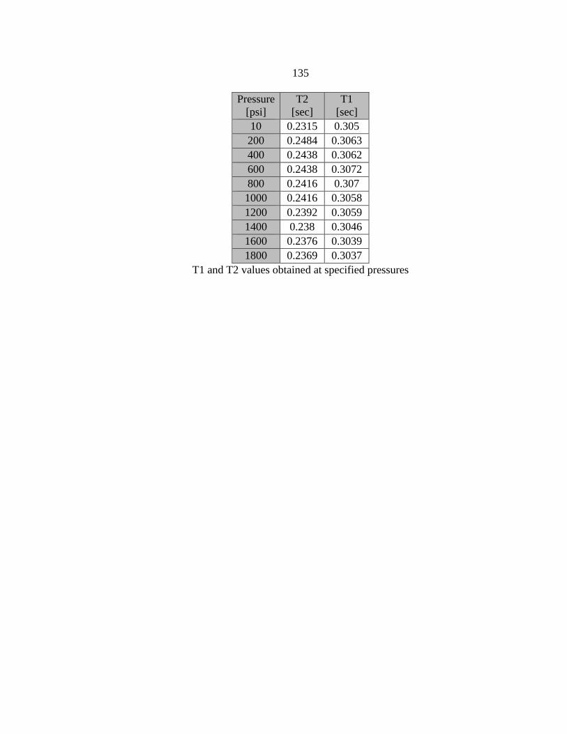
135
Pressure
[psi]
T2
[sec]
T1
[sec]
10 0.2315 0.305
200 0.2484 0.3063
400 0.2438 0.3062
600 0.2438 0.3072
800 0.2416 0.307
1000 0.2416 0.3058
1200 0.2392 0.3059
1400 0.238 0.3046
1600 0.2376 0.3039
1800 0.2369 0.3037
T1 and T2 values obtained at specified pressures

136
APPENDIX C
VISCOUS FINGERING DATA

137
Water displacement by CO2 gas (uncropped)
ZTE image of saturated bead pack
ZTE image of saturated bead pack after pressure inversion incident

138
T2 relaxation map from MSME scans
T2 1D profile for 34 sequential scans
T2 progression for 34 sequential scans at 18 mm (red lines in figures above)

139
T2 progression for 34 sequential scans at 62 mm (blue lines in figures above)
1D average profile for MSME data
1D average profile for ZTE data

140
APPENDIX D
CAPILLARY TRAPPING DATA

141
Scan (Non-
Wetting
Phase)
Normalized 1D Avg. Intensity from 28-54mm
Run
Air
(AFLAS
)
Air
(FEP)
CO2
(FEP)
CO2
(FEP)
scCO2
(FEP)
scCO2
(FEP)
Fully Saturated 0 0 0 0 0 0
Drainage-1 0.00 0.01 0.02 0.02 0.40 0.30
Drainage-2 0.30 0.22 0.36 0.43 0.44 0.40
Drainage-3 0.35 ----- 0.47 0.48 0.49 0.43
Drainage-4
(SInitial)
0.41 0.42 0.51 0.51 0.51 0.47
Imbibition
Final (SResidual)
0.28 0.32 0.36 0.37 0.27 0.30
SResidual/SInitial 0.68 0.76 0.71 0.73 0.53 0.64
Data for rock core #2
Scan (Non-
Wetting
Phase)
Normalized 1D Avg. Intensity from 28-54mm
Run Air
(FEP)
Air
(FEP)
CO2
(FEP)
CO2
(FEP)
scCO2
(FEP)
scCO2
(FEP)
Fully Saturated 0 0 0 0 0 0
Drainage-1 0.10 0.03 0.01 0.04 0.19 0.18
Drainage-2 0.35 0.36 0.34 0.39 0.42 0.40
Drainage-3 0.38 0.40 0.41 0.44 0.44 0.42
Drainage-4
(SInitial)
0.40 0.44 0.47 0.48 0.49 0.48
Imbibition
Final (SResidual)
0.30 0.32 0.33 0.35 0.29 0.29
SResidual/SInitial 0.75 0.73 0.70 0.73 0.59 0.60
Data for rock core #3

142
Scan (Non-
Wetting
Phase)
Average values for all 4 runs of
air, CO2, and scCO2 with
standard deviation
Run Air CO2 scCO2
Drainage-4
(SInitial)
0.42±0.02 0.49±0.02 0.49±0.02
Imbibition
Final (SResidual)
0.31±0.02 0.35±0.02 0.29±0.01
SResidual/SInitial 0.73±0.04 0.72±0.02 0.59±0.05
Summarized averages of all runs on both cores
Initial NW saturation fraction vs. residual NW saturation fraction
Nitrogen Air CO2 scCO2 Water(70F) Water(95F)
Viscosity
[mPa*s]
0.0191 0.0192 0.0723 0.0225 0.972 0.719
Viscosities of fluids

143
Run Air
Water
CO2
Water
scCO2
Water
Surface
Tension
[mN/m]
72 30.84 28.35
Surface tensions of fluids from Bachu et al
Name Ca logCa
Air 2.720E-08 -7.566
CO2 2.391E-07 -6.621
scCO2 8.094E-08 -7.092
Water (Air) 1.377E-06 -5.861
Water (CO2) 3.214E-06 -5.493
Water
(scCO2)
3.497E-06 -5.456
Calculated Ca number for drainage/imbibition of invading fluid
Scan Average Intensity of 2D Plot/1D Avg. 28-54
Integral (10^6) FID Area
M9bs (fully saturated, Soriginal)
730/1320 2.99 12725
M10bs (Drainage-1) 705/1320 2.89 12465
M11bs (Drainage-2) 511/931 2.09 11770
M12bs (Drainage-3) 458/859 1.88 11675
M13bs (Drainage-4) 422/782 1.73 11609
M14bs (Imbibition) 529/955 2.17 11980
M7 (Empty) 10697
Air/water rock core #2, run 1 data

144
Air/water rock core #2, run 1 ZTE data
Scan Average Intensity of 2D Plot/1D Avg. 28-54
Integral FID Area
M23bs (fully saturated, Soriginal)
755/1400 3090000 12180
M24bs (Drainage-1) 747/1390 3060000 12095
M26bs (Drainage-2) 570/1090 2330000 11200
M28bs (End of drainage)
434/815 1780000 10545
M29bs (Imbibition Start)
462/808 1890000 ~10744
M31bs (Imbibition End) 521/952 2130000 11015
M22 (Empty) 9595
Air/water rock core #2, run 2 data

145
Air/water rock core #2, run 2 ZTE data
Scan Average Intensity of 2D Plot/1D Avg. 28-54
Integral (10^6) FID Area
M16bs (fully saturated, Soriginal)
735/1330 3.01 12004
M17bs (Drainage-1) 699/1300 2.86 11918
M18bs (Drainage-2) 493/855 2.02 10995
M20bs (Drainage-3) 388/709 1.59 10400
M21bs (Drainage-4) 353/653 1.44 10280
M23bs (Imbibition) 483/853 1.98 10796
M15 (Empty) 9560
CO2/water rock core #2, run1 data
CO2/water rock core #2, run 1 ZTE data

146
Scan Average Intensity of 2D Plot/1D Avg. 28-54
Integral (10^6) FID Area
M5bs (fully saturated, Soriginal)
703/1260 2.88 11335
M6bs (Drainage-1) 664/1230 2.72 11071
M7bs (Drainage-2) 401/714 1.64 10096
M8bs (Drainage-3) 372/658 1.52 10035
M9bs (Drainage-4) 344/616 1.41 9985
M12bs (Imbibition) 465/799 1.91 10316
M3 (Empty) 9250
CO2/water rock core #2, run 2 data
CO2/water rock core #2, run 2 ZTE data
Scan Average Intensity of 2D Plot/1D Avg. 28-54
Integral (10^6) FID Area
M25bs (fully saturated, Soriginal)
640/1150 2.62 11455
M27bs (Drainage-1) 354/692 1.45 10151
M28bs (Drainage-2) 326/647 1.34 10125
M29bs (Drainage-3) 306/591 1.26 10100
M30bs (Drainage-4) 295/567 1.21 10072
M32bs (Imbibition) 475/843 1.95 10685
M24 (Empty) 9500
scCO2/water rock core #2, run 1 data

147
scCO2/water rock core #2, run1 ZTE data
Scan Average Intensity of 2D Plot /1D Avg 28-54
Integral (10^6) FID Area
M5bs (fully saturated, Soriginal)
635/1220 2.60
M7bs (Drainage-1) 449/854 1.84
M8bs (Drainage-2) 361/732 1.48
M9bs (Drainage-3) 344/694 1.41
M10bs (Drainage-4) 321/652 1.32
M13bs (Imbibition) 460/852 1.88
M4 (Empty)
scCO2/water rock core#2, run 2 data
scCO2/water rock core #2, run 2 ZTE data

148
Scan Average Intensity of 2D Plot / 1D Avg 28-54
Integral (10^6) FID Area
M15bs (fully saturated, Soriginal)
708 / 1340 2.90 11475
M17bs (Drainage-1) 596/1200 2.44 11110
M18bs (Drainage-2) 445/872 1.82 10405
M19bs (Drainage-3) 424/827 1.74 10345
M20bs (Drainage-4) 403 / 801 1.65 10306
M21bs (Imbibition) 501 / 940 2.05 10667
M14 (Empty) 9370
Air/water rock core #3, run 1 data
Air/water rock core #3, run 1 ZTE data
Scan Average Intensity of 2D Plot / 1D Avg 28-54
Integral (10^6) FID Area
M63bs (fully saturated, Soriginal)
712/1350
M65bs (Drainage-1) 631/1310
M66bs (Drainage-2) 450/865
M67bs (Drainage-3) 426/813
M68bs (Drainage-4) 393/757
M69bs (Imbibition) 499/924
M62 (Empty)
Air/water rock core #3, run 2 data
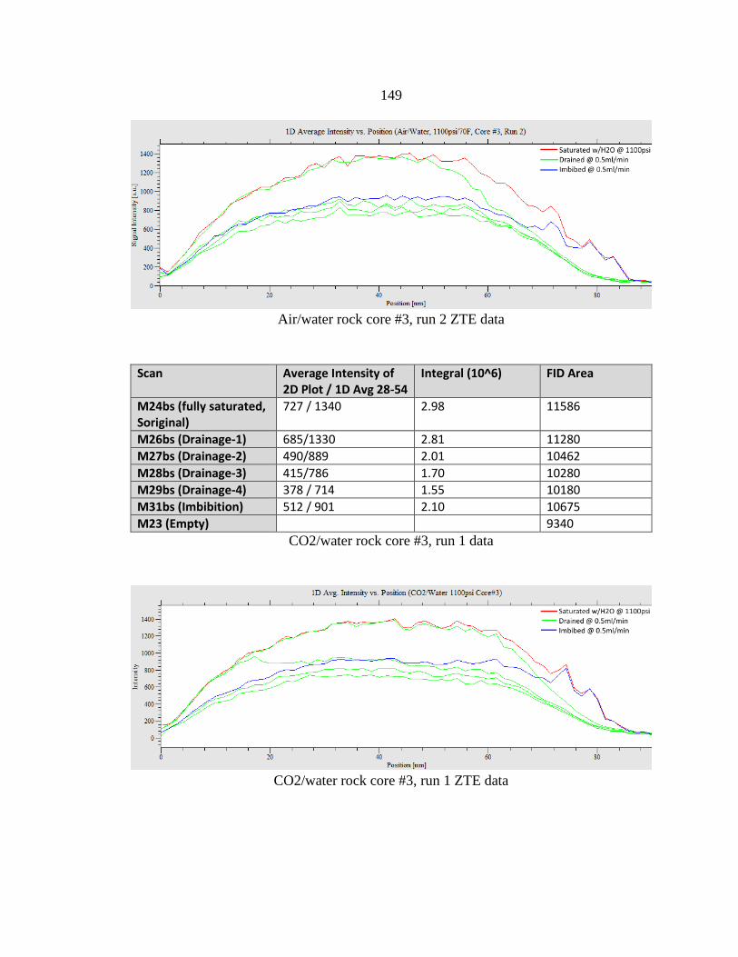
149
Air/water rock core #3, run 2 ZTE data
Scan Average Intensity of 2D Plot / 1D Avg 28-54
Integral (10^6) FID Area
M24bs (fully saturated, Soriginal)
727 / 1340 2.98 11586
M26bs (Drainage-1) 685/1330 2.81 11280
M27bs (Drainage-2) 490/889 2.01 10462
M28bs (Drainage-3) 415/786 1.70 10280
M29bs (Drainage-4) 378 / 714 1.55 10180
M31bs (Imbibition) 512 / 901 2.10 10675
M23 (Empty) 9340
CO2/water rock core #3, run 1 data
CO2/water rock core #3, run 1 ZTE data

150
Scan Average Intensity of 2D Plot / 1D Avg 28-54
Integral (10^6) FID Area
M54bs (fully saturated, Soriginal)
728/1400
M56bs (Drainage-1) 647/1350
M57bs (Drainage-2) 456/858
M58bs (Drainage-3) 394/780
M59bs (Drainage-4) 359/726
M60bs (Imbibition) 479/904
M53 (Empty)
CO2/water rock core #3, run 2 data
CO2/water rock core #3, run 2 ZTE data
Scan Average Intensity of 2D Plot / 1D Avg 28-54
Integral (10^6) FID Area
M34bs (fully saturated, Soriginal)
643 / 1240 2.64 11010
M36bs (Drainage-1) 502/1000 2.06 10750
M37bs (Drainage-2) 360/720 1.47 9880
M38bs (Drainage-3) 342/689 1.40 9815
M39bs (Drainage-4) 313 / 631 1.28 9709
M41bs (Imbibition) 473 / 876 1.94 10199
M33 (Empty) 9130
scCO2/water rock core #3, run 1 data

151
scCO2/water rock core #3, run 1 ZTE data
Scan Average Intensity of 2D Plot / 1D Avg 28-54
Integral (10^6) FID Area
M44bs (fully saturated, Soriginal)
663/1260
M46bs (Drainage-1) 531/1040
M47bs (Drainage-2) 387/759
M48bs (Drainage-3) 363/726
M49bs (Drainage-4) 334/659
M51bs (Imbibition) 489/894
M43 (Empty)
scCO2/water rock core #3, run 2 data
scCO2/water rock core #3, run 2 ZTE data

152
T2 distribution air/water rock core #2, run 1
T2 distribution air/water rock core #2, run 1 zoomed

153
T2 distribution air/water rock core #2, run 2
T2 distribution air/water rock core #2, run 2 zoomed
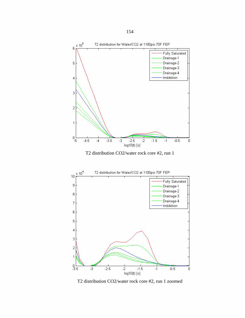
154
T2 distribution CO2/water rock core #2, run 1
T2 distribution CO2/water rock core #2, run 1 zoomed

155
T2 distribution scCO2/water rock core #2, run 1
T2 distribution scCO2/water rock core #2, run 1 zoomed
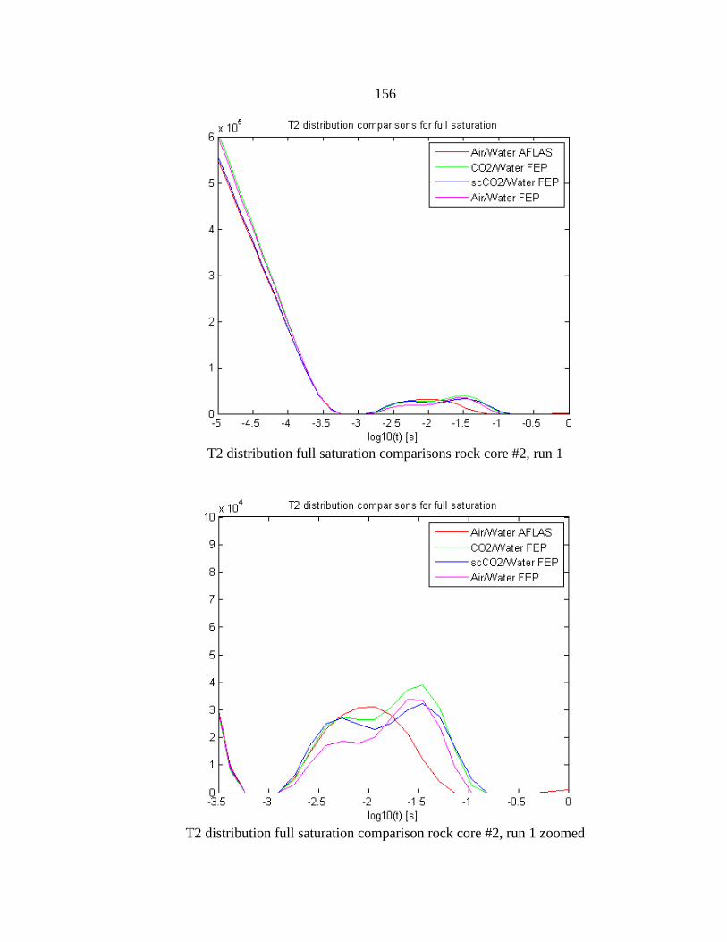
156
T2 distribution full saturation comparisons rock core #2, run 1
T2 distribution full saturation comparison rock core #2, run 1 zoomed

157
T2 distribution drainage comparison rock core #2, run 1
T2 distribution drainage comparison rock core #2, run 1 zoomed

158
T2 distribution imbibition comparison rock core #2, run 1
T2 distribution imbibition comparison rock core #2, run 1 zoomed

159
T2 distribution comparison between air and scCO2 rock core #2
T2 distribution comparison between CO2 and scCO2 rock core #2

160
T2 distribution air/water rock core #3, run 1
T2 distribution air/water rock core #3, run 2
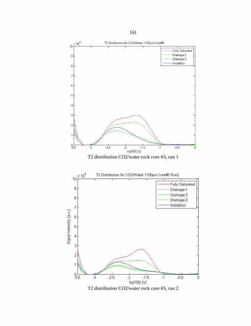
161
T2 distribution CO2/water rock core #3, run 1
T2 distribution CO2/water rock core #3, run 2

162
T2 distribution scCO2/water rock core #3, run 1
T2 distribution scCO2/water rock core #3, run 2

163
T2 distribution 5 mm core vs, 27 mm core

164
APPENDIX E
TWO PHASE FLOW DATA
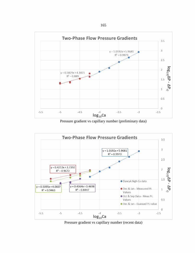
165
Pressure gradient vs capillary number (preliminary data)
Pressure gradient vs capillary number (recent data)

166
FID and pressure data for flow rate = 0.595 ml/min
MSME and pressure data for flow rate = 0.595 ml/min

167
FID and pressure data for flow rate = 0.188 ml/min
MSME and pressure data for flow rate = 0.188 ml/min