nmath stats user's guide - centerspace software
TRANSCRIPT
NMath StatsUser’s Guide
Version 4.2

NMATH STATS USER’S GUIDE
© 2016 Copyright CenterSpace Software, LLC. All Rights Reserved.
The correct bibliographic reference for this document is:NMath Stats User’s Guide, Version 4.2, CenterSpace Software, Corvallis, OR. Printed in the United States.Printing Date: March, 2016
CENTERSPACE SOFTWARE
Address: 622 NW 32nd St., Corvallis, OR 97330 USAPhone: (541) 896-1301Web: http://www.centerspace.net
Technical Support: [email protected]
CONTENTS
Chapter 1. Introduction .......................................................................................................1
1.1 Product Features...........................................................................................1
1.2 Software Requirements...........................................................................2
1.3 Namespaces .......................................................................................................3
1.4 Building and Deploying NMath Stats Applications .........3
1.5 Documentation ...............................................................................................4
This Manual 4
1.6 Visualization.......................................................................................................5
1.7 Technical Support ........................................................................................6
Chapter 2. Data Frames ......................................................................................................7
2.1 Column Types ..................................................................................................8
Creating Columns 8Adding and Removing Data 9Accessing Column Data 10Column Properties 10Reordering Column Data 11Missing Values 11Transforming Column Data 12Exporting Column Data 14
2.2 Creating DataFrames............................................................................. 14
Creating Empty DataFrames 14Creating DataFrames from Arrays of Columns 15Creating DataFrames from Matrices 15Creating DataFrames from ADO.NET Objects 15Creating DataFrames from Strings 16
iii
2.3 Adding and Removing Columns ....................................................17
2.4 Adding and Removing Rows .............................................................18
Modifying Row Keys 20
2.5 Properties of DataFrames ..................................................................21
2.6 Accessing DataFrames...........................................................................21
Accessing Elements 21Accessing Columns 21Accessing Rows 22
2.7 Subsets .................................................................................................................23
Creating Subsets 24Properties of Subsets 25Accessing Elements 25Logical Operations on Subsets 25Arithmetic Operations on Subsets 26Manipulating Subsets 26Groupings 27Random Samples 27
2.8 Accessing Sub-Frames ...........................................................................28
2.9 Reordering DataFrames .......................................................................29
Sorting Rows 29Permuting Rows and Columns 30
2.10 Factors..................................................................................................................30
Creating Factors 31Properties of Factors 31Accessing Factors 32Creating Groupings with Factors 32
2.11 Cross-Tabulation.........................................................................................34
Column Delegates 35Applying Column Delegates to Tabulated Data 35
2.12 Exporting Data from DataFrames ..............................................37
Exporting to a Matrix 37Exporting to a String 37Exporting to an ADO.NET DataTable 39Binary and SOAP Serialization 39
iv NMath Stats User’s Guide

Chapter 3. Descriptive Statistics ........................................................................41
3.1 Column Types................................................................................................41
3.2 Missing Values ................................................................................................43
3.3 Counts and Sums ........................................................................................44
3.4 Min/Max Functions .....................................................................................45
3.5 Ranks, Percentiles, Deciles, and Quartiles ...........................45
3.6 Central Tendency .......................................................................................46
3.7 Spread ...................................................................................................................48
3.8 Shape......................................................................................................................49
3.9 Covariance, Correlation, and Autocorrelation ................50
3.10 Sorting ..................................................................................................................51
3.11 Logical Functions ........................................................................................51
Chapter 4. Probability Distributions ............................................................53
4.1 Distribution Classes ..................................................................................53
Beta Distribution 55Binomial Distribution 56Chi-Square Distribution 56Exponential Distribution 57F Distribution 58Gamma Distribution 58Geometric Distribution 59Johnson Distribution 59Logistic Distribution 61Log-Normal Distribution 62Negative Binomial Distribution 62Normal Distribution 63Poisson Distribution 63Student’s t Distribution 64Triangular Distribution 65Uniform Distribution 65Weibull Distribution 66
v

4.2 Correlated Random Inputs ................................................................67
Constructing Correlator Instances 67Correlating Random Inputs 68Correlator Properties 68Convenience Method 69
4.3 Box-Cox Power Transformations ................................................69
Chapter 5. Hypothesis Tests ......................................................................................71
5.1 Common Interface ....................................................................................71
Static Properties 71Creating Hypothesis Test Objects 72Properties of Hypothesis Test Objects 73Modifying Hypothesis Test Objects 74Printing Results 74
5.2 One Sample Z-Test...................................................................................75
5.3 One Sample T-Test ..................................................................................77
5.4 Two Sample Paired T-Test................................................................79
5.5 Two Sample Unpaired T-Test ........................................................81
5.6 Two Sample F-Test...................................................................................83
5.7 Pearson’s Chi-Square Test .................................................................85
5.8 Fisher’s Exact Test ....................................................................................87
Chapter 6. Linear Regression...................................................................................89
6.1 Creating Linear Regressions .............................................................89
Parameter Calculation by Least Squares Minimization 90Intercept Parameters 91
6.2 Regression Results .....................................................................................91
Variance Inflation Factor 92
6.3 Predictions ........................................................................................................92
6.4 Accessing and Modifying the Model ...........................................93
Accessing and Modifying Predictors 93
vi NMath Stats User’s Guide

Accessing and Modifying Observations 95Accessing and Modifying the Intercept Option 96Updating the Entire Model 96
6.5 Significance of Parameters .................................................................97
Creating Linear Regression Parameter Objects 97Properties Linear Regression Parameters 97Hypothesis Tests 97Updating Linear Regression Parameters 98
6.6 Significance of the Overall Model.................................................98
Chapter 7. Logistic Regression ........................................................................... 101
7.1 Regression Calculators........................................................................ 101
7.2 Creating Logistic Regressions....................................................... 102
Design Variables 103
7.3 Checking for Convergence .............................................................. 104
7.4 Goodness of Fit .......................................................................................... 104
7.5 Parameter Estimates ........................................................................... 105
7.6 Predicted Probabilities........................................................................ 106
7.7 Auxiliary Statistics .................................................................................. 107
Chapter 8. Analysis of Variance......................................................................... 109
8.1 One-Way ANOVA.................................................................................. 109
Creating One-Way ANOVA Objects 109The One-Way ANOVA Table 110Grand Mean, Group Means, and Group Sizes 111Critical Value of the F Statistic 112Updating One-Way ANOVA Objects 112
8.2 One-Way Repeated Measures ANOVA .............................. 113
Creating One-Way RANOVA Objects 113The One-Way RANOVA Table 114Grand Mean, Subject Means, and Treatment Means 115Critical Value of the F Statistic 115Updating One-Way RANOVA Objects 115
vii
8.3 Two-Way Balanced ANOVA .........................................................116
Creating Two-Way ANOVA Objects 116The Two-Way ANOVA Table 116Cell Data 118Grand Mean, Cell Means, and Group Means 118ANOVA Regression Parameters 118
8.4 Two-Way Unbalanced ANOVA ..................................................123
Creating UnbalancedTwo-Way ANOVA Objects 124Unbalanced Two-Way ANOVA Tables and Regression Parameters 124
8.5 Two-Way Repeated Measures ANOVA .............................125
Creating Two-Way RANOVA Objects 125Two-Way RANOVA Tables 125
Chapter 9. Non-Parametric Tests...................................................................129
9.1 One Sample Kolmogorov-Smirnov Test .............................129
9.2 Two Sample Kolmogorov-Smirnov Test.............................130
9.3 Shapiro-Wilk Test ....................................................................................131
9.4 One Sample Anderson-Darling Test .......................................132
9.5 Kruskal-Wallis Test.................................................................................132
Creating Kruskal-Wallis Objects 132The Kruskal-Wallis Table 133Ranks, Grand Mean Ranks, Group Means Ranks, and Group Sizes 135Critical Value of the Test Statistic 136Updating Kruskal-Wallis Test Objects 136
Chapter 10. Multivariate Techniques ........................................................137
10.1 Principal Component Analysis......................................................137
Creating Principal Component Analyses 137Principal Component Analysis Results 138
10.2 Factor Analysis............................................................................................139
Creating Factor Analyses 140Factor Analysis Results 141Factor Scores 143
viii NMath Stats User’s Guide
10.3 Hierarchical Cluster Analysis ........................................................ 144
Distance Functions 144Linkage Functions 146Creating Cluster Analyses 147Cluster Analysis Results 148Reusing Cluster Analysis Objects 150
10.4 K-Means Clustering ................................................................................ 151
Creating KMeansClustering Objects 151Stopping Criteria 151Clustering 152Cluster Analysis Results 152
Chapter 11. Nonnegative Matrix Factorization ..................... 155
11.1 Nonnegative Matrix Factorization ........................................... 155
Update Algorithms 156
11.2 Data Clustering Using NMF ........................................................... 158
Creating NMFClustering Instances 159Performing the Factorization 159Cluster Results 159Computing a Consensus Matrix 161
Chapter 12. Partial Least Squares ................................................................ 165
12.1 Computing a PLS Regression........................................................ 166
12.2 Error Checking........................................................................................... 166
12.3 Predicted Values....................................................................................... 167
12.4 Analysis of Variance............................................................................... 167
12.5 PLS Algorithms ......................................................................................... 168
12.6 Cross Validation ........................................................................................ 169
Jackknifing of Regression Coefficients 170
12.7 Partial Least Squares Discriminant Analysis................... 171
ix

Chapter 13. Goodness of Fit ....................................................................................173
13.1 Significance of the Overall Model...............................................173
13.2 Significance of Parameters...............................................................175
Creating Goodness of Fit Parameter Objects 175Properties of Goodness of Fit Parameters 175Hypothesis Tests 176
Chapter 14. Process Control...................................................................................177
14.1 Process Capability....................................................................................177
14.2 Process Performance ............................................................................178
14.3 Z Bench..............................................................................................................178
Index ...................................................................................................................................................................181
x NMath Stats User’s Guide

CHAPTER 1. INTRODUCTION
Welcome to the NMath Stats User’s Guide.
NMath Stats is part of CenterSpace Software’s NMath™ product suite, which provides object-oriented components for mathematical, engineering, scientific, and financial applications on the .NET platform. NMath Stats provides functions for statistical computation, including descriptive statistics, probability distributions, combinatorial functions, multiple linear regression, hypothesis testing, and analysis of variance.
Fully compliant with the Microsoft Common Language Specification, all NMath Stats routines are callable from any .NET language, including C#, Visual Basic, and Managed C++.
1.1 Product Features
The features of NMath Stats include:
A data frame class for holding data of various types (numeric, string, boolean, datetime, and generic), with methods for appending, inserting, removing, sorting, and permuting rows and columns.
Functions for computing descriptive statistics, such as mean, variance, standard deviation, percentile, median, quartiles, geometric mean, harmonic mean, RMS, kurtosis, skewness, and many more.
Probability density function (PDF), cumulative distribution function (CDF), inverse CDF, and random variable moments for a variety of probability distributions.
Multiple linear regression and logistic regression.
Basic hypothesis tests, such as z-test, t-test, F-test, and Pearson’s chi-square test, with calculation of p-values, critical values, and confidence intervals.
Chapter 1. Introduction 1

One-way and two-way analysis of variance (ANOVA) and analysis of variance with repeated measures (RANOVA).
Non-parametric tests, such as the Kolmogorov-Smirnov test and Kruskal-Wallis rank sum test.
Multivariate statistical analyses, including principal component analysis, factor analysis, hierarchical cluster analysis, and k-means cluster analysis.
Nonnegative matrix factorization (NMF), and data clustering using NMF.
Partial least squares (PLS).
Statistical process control.
Visualization using the Microsoft Chart Controls for .NET.
1.2 Software Requirements
NMath Stats requires the following additional software to be installed on your system:
NMath Stats depends on NMath, the foundational library in the NMath product suite. NMath must be installed on your system prior to building or executing NMath Stats code.
To use the NMath Stats library, you need the Microsoft .NET Framework installed on your system. The .NET Framework is available without cost from:
http://msdn.microsoft.com/netframework
Use of Microsoft Visual Studio .NET (or other .NET IDE) is strongly encouraged. However, the .NET Framework includes command line compilers for .NET languages, so an IDE is not strictly required.
Viewing PDF documentation requires Adobe Acrobat Reader, available without cost from:
http://www.adobe.com
2 NMath Stats User’s Guide
1.3 Namespaces
All types in NMath Stats are in the CenterSpace.NMath.Stats namespace. To avoid using fully qualified names, preface your code with an appropriate namespace statement. For example:
Code Example – C#
using CenterSpace.NMath.Stats;
Code Example – VB
imports CenterSpace.NMath.Stats
All NMath Stats code shown in this manual assumes the presence of such a namespace statement.
NOTE—In most cases, you must also preface your code with a namespace statement for the CenterSpace.NMath.Core namespace.
1.4 Building and Deploying NMath Stats Applications
The NMath Stats installer places assembly NMathStats.dll in directory <installdir>/Assemblies, and in your global assembly cache. To use NMath Stats types in your application, add a reference to NMathStats.dll.
NMath Stats depends on NMath, the foundational library in the NMath product suite, so you must also add a reference to NMath.dll, as described in the NMath User’s Guide.
You can build your application using the Any CPU build configuration, and deploy to either 32-bit or 64-bit environments. (If you are building for .NET 4.5 or higher, also ensure that the Prefer 32-bit flag is unchecked, under Build | Platform target in your project properties.)
NOTE—A valid license key must accompany your deployed NMath Stats code. For more information, see “NMath License Key” in the NMath User’s Guide.
Chapter 1. Introduction 3
1.5 Documentation
NMath Stats includes the following documentation:
The NMath Stats User’s Guide (this manual)
This document contains an overview of the product, and instructions on how to use it. You are encouraged to read the entire User’s Guide. The NMath Stats User’s Guide is installed in:
installdir/Docs/NMath.Stats.UsersGuide.pdf
An HTML version of the NMath Stats User’s Guide may be viewed online using your browser at:
http://www.centerspace.net/doc/NMathStats/user
The NMath Stats Reference
This document contains complete API reference documentation in com-piled HTML Help format, enabling you to browse the NMath Stats library just like the .NET Framework Class Library. The NMath Stats Reference is installed in:
installdir/Docs/NMath.Stats.Reference.chm
NOTE—Links to types in the .NET Framework will be broken unless you have the .NET Framework installed on your machine.
HTML reference documentation may be viewed online using your browser at:
http://www.centerspace.net/doc/NMathSuite/ref
A readme file
This document describes the results of the installation process, how to build and run code examples, and lists any late-breaking product issues. The readme file is installed in:
installdir/readme.txt
This Manual
This manual assumes that you are familiar with the basics of .NET programming and object-oriented technology.
Most code examples in this manual use C#; a few are shown in Visual Basic. However, all NMath Stats routines are callable from any .NET language.
4 NMath Stats User’s Guide

This manual uses the following typographic conventions:
1.6 Visualization
NMath Stats can be easily combined with the free Microsoft Chart Controls for .NET to create a complete data analysis and visualization solution. The Microsoft Chart Controls for .NET are available as a separate download for .NET 3.5. Beginning in .NET 4.0, the Chart controls are part of the .NET Framework.
NMath Stats provides convenience methods for plotting NMath Stats types using the Microsoft Chart Controls. For example, this code plots the probability density function (PDF) of the specified gamma distribution:
Code Example – C# charts
double alpha = 9.0;double beta = 0.5;var gamma = new GammaDistribution( alpha, beta );
NMathStatsChart.Show( gamma, NMathStatsChart.DistributionFunction.PDF );
Table 1 – Typographic conventions
Convention Purpose Example
Courier Function names, code, direc-tories, file names, examples, and operating system commands.
FDistribution.CDF()
the Assemblies directory
italic Conventional uses, such as emphasis and new terms.
The entries along the diagonal are the singular values.
bold Class names, product names, and commands from an interface.
TwoSamplePairedTTest
NMath Stats
Click OK.
Chapter 1. Introduction 5
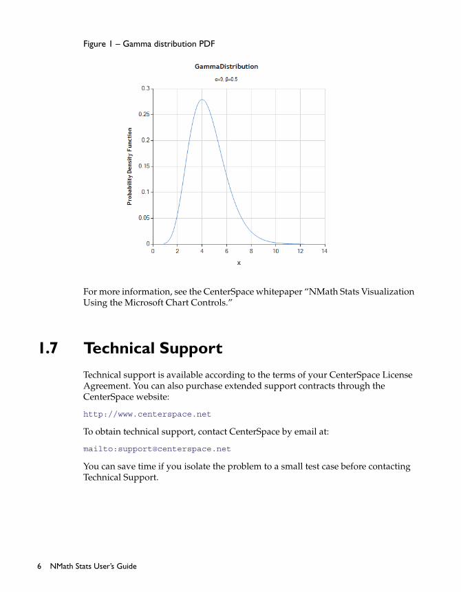
Figure 1 – Gamma distribution PDF
For more information, see the CenterSpace whitepaper “NMath Stats Visualization Using the Microsoft Chart Controls.”
1.7 Technical Support
Technical support is available according to the terms of your CenterSpace License Agreement. You can also purchase extended support contracts through the CenterSpace website:
http://www.centerspace.net
To obtain technical support, contact CenterSpace by email at:
mailto:[email protected]
You can save time if you isolate the problem to a small test case before contacting Technical Support.
6 NMath Stats User’s Guide

CHAPTER 2. DATA FRAMES
The statistical functions in NMath Stats support the NMath types DoubleVector and DoubleMatrix, as well as simple arrays of doubles. In many cases, these types are sufficient for storing and manipulating your statistical data. However, they suffer from two limitations: they can only store numeric data, and they have limited support for adding, inserting, removing, and reordering data. Because the underlying data is an array of doubles, data must be copied to new storage every time manipulation operations such as these are performed.
For these reasons, NMath Stats provides the DataFrame class which represents a two-dimensional data object consisting of a list of columns of the same length. Columns are themselves lists of different types of data: numeric, string, boolean, generic, and so on.
Methods are provided for appending, inserting, removing, sorting, and permuting rows and columns in a data frame. Because the underlying data is in a list, elements can be added, removed, and reordered without having to copy all of the data to new storage.
A DataFrame can be viewed as a kind of virtual database table. Columns can be accessed by numeric index (0...n-1) or by a string name supplied at construction time. Rows can be accessed by numeric index (0...n-1) or by a key object. Column names and row keys do not need to be unique. For example, this output shows a formatted string representation of data from a sample data frame:
# State Weight MarriedJohn Smith OR 165 trueRuth Barnes WA 147 trueJane Jones VT 115 falseTim Travis AK 230 falseBetsy Young MA 130 trueArthur Smith CA 152 falseEmma Allen OK 135 falseRoy Wilkenson WI 182 true
Chapter 2. Data Frames 7
This data frame contains three columns: column 0, named State, contains string data; column 1, named Weight, contains integer data; column 2, named Married, contains boolean data. There are eight rows of data in this data frame, and the subjects’ names are used as row keys.
This chapter describes how to use the DataFrame class.
2.1 Column Types
A DataFrame may contain columns of different types—the only constraint is that the columns must be of the same length. DFColumn, which implements the IDFColumn interface, is the abstract base class for data frame columns. NMath Stats provides the following derived classes for column types:
DFBoolColumn represents a column of logical data.
DFDateTimeColumn represents a column of temporal data.
DFGenericColumn represents a column of generic data.
DFIntColumn represents a column of integer data.
DFNumericColumn represents a column of double-precision floating point data.
DFStringColumn represents a column of string data.
Creating Columns
Empty columns are constructed by simply supplying a name for the column. For example:
Code Example – C#
var col = new DFDateTimeColumn( “myCol” );
The name of a column can be used to access the column in a data frame. Once a column instance is constructed, the name cannot be changed.
NOTE—Columns also provide a modifiable Label property for display purposes; see below.
8 NMath Stats User’s Guide
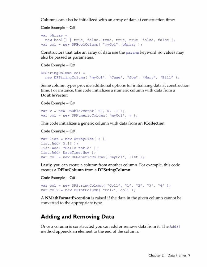
Columns can also be initialized with an array of data at construction time:
Code Example – C#
var bArray = new bool[] { true, false, true, true, true, false, false };var col = new DFBoolColumn( “myCol”, bArray );
Constructors that take an array of data use the params keyword, so values may also be passed as parameters:
Code Example – C#
DFStringColumn col = new DFStringColumn( “myCol”, “Jane”, “Joe”, “Mary”, “Bill” );
Some column types provide additional options for initializing data at construction time. For instance, this code initializes a numeric column with data from a DoubleVector:
Code Example – C#
var v = new DoubleVector( 50, 0, .1 );var col = new DFNumericColumn( "myCol", v );
This code initializes a generic column with data from an ICollection:
Code Example – C#
var list = new ArrayList( 3 );list.Add( 3.14 );list.Add( "Hello World" );list.Add( DateTime.Now );var col = new DFGenericColumn( "myCol", list );
Lastly, you can create a column from another column. For example, this code creates a DFIntColumn from a DFStringColumn:
Code Example – C#
var col = new DFStringColumn( “Col1”, “1”, “2”, “3”, “4” );var col2 = new DFIntColumn( “Col2”, col1 );
A NMathFormatException is raised if the data in the given column cannot be converted to the appropriate type.
Adding and Removing Data
Once a column is constructed you can add or remove data from it. The Add() method appends an element to the end of the column:
Chapter 2. Data Frames 9
Code Example – C#
var col = new DFStringColumn( “Name” );col.Add( “Joe Smith” );col.Add( “Jane Doe” );col.Add( “John Davis” );
The Insert() method inserts an element into a column at a given index. For instance, this code insert a new element at the top of the column:
Code Example – C#
col.Insert( 0, “Sally Jones” );
The RemoveAt() method removes the element at a given index:
Code Example – C#
col.RemoveAt( 3 );
Accessing Column Data
The data frame column classes provide standard indexing operators for getting and setting element values. Thus, col[i] always returns the ith element of the column:
Code Example – C#
DFStringColumn col = new DFStringColumn( “Names”, “Jane”, “Joe”, “Mary”, “Bill” );col[0] = “Janet”;
The GetEnumerator() method returns an enumerator for the column data:
Code Example – C#
IEnumerator enumerator = col.GetEnumerator();while ( enumerator.MoveNext() ){ // Do something with enumerator.Current}
Column Properties
Data frame column types provide the following properties:
ColumnType gets the type of the objects held by the column.
Count gets the number of ojects in the column.
10 NMath Stats User’s Guide
IsNumeric returns true if a column is of type DFIntColumn or DFNumericColumn.
Label gets and sets the label in the header of the column.
MissingValue gets and sets the value used to represent missing values in the column (see below).
Name gets the name of the column.
NOTE—The Name of a column can only be set in a constructor. Once a column is con-structed, the name cannot be changed. For a modifiable label, see the Label property.
Reordering Column Data
You can use the Permute() method to arbitrarily reorder the elements in a column. This method accepts a permutation array of element indices and reorders the elements such that this[ permutation[i] ] is set to the ith object in the original column.
For example, this code moves the last two elements to the head of the column:
Code Example – C#
DFStringColumn col = new DFStringColumn( "myCol", "a", "b", "c", "d", "e" );col.Permute( 2, 3, 4, 0, 1 );
Missing Values
All column types—except DFBoolColumn, which has only two valid values—support missing values. Most statistical functions in NMath Stats are accompanied by a paired function that ignores missing values (Section 3.2).
NOTE—To represent missing values in boolean data, use a DFIntColumn. For example, use 1 for true, 0 for false, and -1 for missing.
At construction time, the missing value for a column is defined using a static variable in class StatsSettings, as shown in Table 2.
Table 2 – Default missing values for data frame column types
Column Type StatsSettings Variable Default Value
DFDateTimeColumn DateTimeMissingValue DateTime.MinValue
DFGenericColumn GenericMissingValue null
DFIntColumn IntegerMissingValue int.MinValue
Chapter 2. Data Frames 11

For instance, this code computes the mean of a column of integers, ignoring any missing values:
Code Example – C#
var col = new DFIntColumn( “myCol”, 5, 2, -1, 1, 0, 7 );double mean = StatsFunctions.NaNMean( col );
By default, a missing value in a DFIntColumn is represented using the default setting of StatsFunctions.IntegerMissingValue, which is int.MinValue. You can change the way a missing value is represented for a particular column instance using the MissingValue property:
Code Example – C#
col.MissingValue = -1;double mean = StatsFunctions.NaNMean( col );
In this example, all values in col equal to -1 are ignored when computing the mean.
NOTE—For DFNumericColumn instances you can use the MissingValue property to indicate that missing values are represented by something other than the default value Double.NaN. However, Double.NaN will continue to be treated as missing, in addition to whatever value you set.
You can also change the default missing value for all columns of a particular type by setting the appropriate static variable in StatsSettings. Thus, this code sets the default missing value for integer columns to -1 for all subsequently constructed DFIntColumn instances:
Code Example – C#
StatsSettings.IntegerMissingValue = -1;
The Clean() method returns a new column with missing values removed.
Transforming Column Data
NMath Stats provides convenience methods for applying functions to elements of a column. Each of these methods takes a function delegate. The Apply() method returns a new column whose contents are the result of applying the given function
DFNumericColumn NumericMissingValue Double.NaN
DFStringColumn StringMissingValue “.”
Table 2 – Default missing values for data frame column types
Column Type StatsSettings Variable Default Value
12 NMath Stats User’s Guide

to each element of the column. The Transform() method modifies a column object by applying the given function to each of its elements.
Suppose, for example, that you want to cap all numeric values in a DFNumericColumn at 100.0. You could write a simple function like this:
Code Example – C#
private static double Cap( double x ){ return x > 100.0 ? 100.0 : x;}
Then encapsulate the function in a Func<double, double> delegate:
Code Example – C#
Func<double, double> capDelegate = new Func<double, double>( Cap );
This code caps all numeric values in column col:
Code Example – C#
col.Transform( capDelegate );
A common use of the Apply() functions is to create a new column whose values are a function of values in one or two existing column. For example, suppose you have FirstName and LastName string columns in data frame df, and want to create a new column containing customers’ full names. You could write a simple function like this:
Code Example – C#
private static string Cat( string first, string last ){ return first + " " + last;}
Then encapsulate the function in a Func<String, String, String> delegate:
Code Example – C#
Func<String, String, String> catDelegate = new Func<String, String, String>( Cat );
This code creates a new column containing the concatenated names:
Code Example – C#
DFStringColumn col = ( (DFStringColumn)data["FirstName"] ).Apply( “FullName”, catDelegate, (DFStringColumn)data["LastName"] );
Chapter 2. Data Frames 13

Exporting Column Data
Data from a column can be exported in various ways:
ToArray() exports the contents of a column to a strongly-typed array.
ToDoubleArray() extracts the contents of a column to an array of doubles (numeric columns only).
ToDoubleVector() extracts the contents of a column to a DoubleVector (numeric columns only).
ToIntArray() extracts the contents of a column to an array of integers (integer columns only).
ToString() returns a formatted string representation of a column.
ToStringArray() exports the contents of a column to an array of strings.
2.2 Creating DataFrames
Data frames can be constructed in a variety of ways.
Creating Empty DataFrames
The default constructor creates an empty data frame with no rows or columns. Columns and rows can then be added to the new data frame.
Code Example – C#
var df = new DataFrame();
// Add some columnsdf.AddColumn( new DFStringColumn( "Sex" )); df.AddColumn( new DFStringColumn( "AgeGroup" ));df.AddColumn( new DFIntColumn( "Weight" ) );
// Add some rowsdf.AddRow( "John Smith", "M", "Child", 45 );df.AddRow( "Ruth Barnes", "F", "Senior", 115 );df.AddRow( "Jane Jones", "F", "Adult", 115 );df.AddRow( "Timmy Toddler", "M", "Child", 42 );df.AddRow( "Betsy Young", "F", "Adult", 130 );df.AddRow( "Arthur Smith", "M", "Senior", 142 );df.AddRow( "Lucy Doe", "F", "Child", 30 );df.AddRow( "Emma Allen", "F", "Child", 35 );
14 NMath Stats User’s Guide

NOTE—The first parameter to the AddRow() method is the row key. See Section 2.3 and Section 2.4, respectively, for more information on adding columns and rows to a data frame.
Creating DataFrames from Arrays of Columns
You can also construct and populate columns independently, then combine them into a data frame:
Code Example – C#
var col1 = new DFNumericColumn( "Col1", 1.1, 2.2, 3.3, 4.4 );var col2 = new DFBoolColumn ( "Col2", true, true, false, true );var col3 = new DFStringColumn ( "Col3", "John", "Paulo", "Sam", "Becky" );var cols = new DFColumn[] { col1, col2, col3 };var df = new DataFrame( cols );
An InvalidArgumentException is thrown if the columns are not all of the same length.
In this case, the row keys are set to nulls; they can later be initialized using the SetRowKeys() method. Alternatively, you can pass in a collection of row keys at construction time:
Code Example – C#
var keys = new object[] { "Row1", "Row2", "Row3", "Row4" };var df = new DataFrame( cols, keys );
Creating DataFrames from Matrices
You can construct a data frame from a DoubleMatrix and an array of column names. A new DFNumericColumn is added for each column in the matrix. For instance, this code creates a data frame from an 8 x 3 matrix:
Code Example – C#
var A = new DoubleMatrix( 8, 3, 0, 1 );var colNames = new string[] { "A", "B", "C" };var df = new DataFrame( A, colNames );
The number of column names must match the number of columns in the matrix.
Creating DataFrames from ADO.NET Objects
You can construct a data frame from an ADO.NET DataTable. For example, assuming table is a DataTable instance:
Chapter 2. Data Frames 15

Code Example – C#
var df = new DataFrame( table );
In this case, the row keys are set to the default rowIndex + 1—that is, 1...n. You can also specify the row keys in various ways. This code passes in an array of row keys:
Code Example – C#
var keys = new object[] { “Row1”, “Row2”, “Row3”, “Row4” };var df = new DataFrame( table, keys );
Alternatively, you can indicate a column in the DataTable, either by column index or column name, to use for the row keys. This code uses column ID for row keys:
Code Example – C#
var df = new DataFrame( table, "ID" );
Creating DataFrames from Strings
You can construct a data frame from a string representation. For example, if str is a tab-delimited string containing:
Code Example – C#
Key Col1 Col2 Col3Row1 1.1 true ARow2 2.2 true BRow3 3.3 false ARow4 4.4 true C
Then you could construct a data frame like so:
var df = new DataFrame( str );
For more control, you can also indicate:
whether the first row of data contains column headers
whether the first column of data contains row keys
the delimiter used to separate columns
whether to parse the column types, or to treat everything as string data
16 NMath Stats User’s Guide

For example, if str is a comma-delimited string containing column headers but no row keys:
Code Example – C#
Col1,Col2,Col31.1,true,A2.2,true,B3.3,false,A4.4,true,C
you could construct a data frame like so:
Code Example – C#
var df = new DataFrame( str, true, false, “,”, true );
2.3 Adding and Removing Columns
The AddColumn() method adds a column to a data frame:
Code Example – C#
var df = new DataFrame();var col = new DFNumericColumn( “myCol” );df.AddColumn( col );
NOTE—The AddColumn() method raises a MismatchedSizeException if you attempt to add a column that is not the same length as any existing columns in a data frame.
You can also add all the columns from one data frame to another, optionally copying the data in the columns. For example, assuming df is a data frame, this code adds the columns of df to a new data frame and copies all the column data:
Code Example – C#
var df2 = new DataFrame();df2.AddColumns( df, true );
Overloads of AddColumn() and AddColumns() accept ADO.NET DataColumn and DataColumnCollection instances, respectively. If the data frame already contains rows of data, you must also pass in a DataRowCollection of the same Count as the number of rows in the data frame.
Chapter 2. Data Frames 17

InsertColumn() inserts a column at a given column index. This code adds a column in the first position:
Code Example – C#
var col = new DFStringColumn( “myCol” );df.InsertColumn( 0, col );
RemoveColumn() removes the column at a given index:
Code Example – C#
df.RemoveColumn( 3 );
You can also identify a column by name:
Code Example – C#
df.RemoveColumn( “myCol” );
Because column names are not constrained to be unique, this method will remove all columns in the data frame with the given name.
RemoveAllColumns() removes all columns from a data frame, but preserves the existing row keys. RemoveColumns() removes the columns specified in a given subset or slice.
Clear() method removes all columns and rows from a data frame. CleanCols() returns a new data frame containing only those columns in a data frame that do not contain missing values.
2.4 Adding and Removing Rows
The AddRow() method adds a row of data to a data frame. The first parameter is the row key; subsequent parameters are the row data. For example:
Code Example – C#
var df = new DataFrame();df.AddColumn( new DFStringColumn( "Col1" )); df.AddColumn( new DFNumericColumn( "Col2" ) );df.AddColumn( new DFNumericColumn( "Col3" ) );df.AddRow( 1546, "Test1", 1.5445, 667.87 );
NOTE—The AddRow() method raises a MismatchedSizeException if the number of row elements does not match the number of columns in the data frame.
This example uses 1546 as an integer row key, perhaps representing some sort of ID. Row keys can be any object, and need not be unique.
18 NMath Stats User’s Guide

Additional overloads of AddRow() accept data in various collections other than an array of objects. One overload takes an ICollection. For instance:
Code Example – C#
var myQ = new Queue();myQ.Enqueue( "Hello" );myQ.Enqueue( 47.0 );myQ.Enqueue( -0.34 );df.AddRow( "Row1", myQ );
Another overload accepts an IDictionary in which the keys are the column names and the values are the row data:
Code Example – C#
var df = new DataFrame();df.AddColumn( new DFNumericColumn( "V1" ) );df.AddColumn( new DFBoolColumn( "V2" ) );df.AddColumn( new DFStringColumn( "V3" ) );var myHT = new Hashtable();myHT.Add( "V1", 3.14 );myHT.Add( "V3", "Hello");myHT.Add( "V2", true );df.AddRow( "Row1", myHT );
If all of the columns in your data frame are numeric, you can add a row as a DoubleVector:
Code Example – C#
var v = new DoubleVector( 10, 0, 1 );df.AddRow( “myKey”, v );
Other overloads of AddRow() and AddRows() accept ADO.NET DataRow and DataRowCollection instances, respectively.
InsertRow() inserts a row at a given row index. For example, this code inserts a row into the second position:
Code Example – C#
var df = new DataFrame();df.AddColumn( new DFNumericColumn( "Col1" ) );df.AddColumn( new DFNumericColumn( "Col2" ) );df.AddColumn( new DFNumericColumn( "Col3" ) );df.AddRow( "Row1", 2.5, 0.0, 3.4 );df.AddRow( "Row2", 3.14, -.5, -.33 );df.AddRow( "Row3", 0.1, 55.34, 12.02 );df.AddRow( "Row4", 3.14, -33.2, 7.22 );var myRow = object[] { 5.5, 9.05, -6.11 };df.InsertRow( 1, "Row1a", myRow );
Chapter 2. Data Frames 19
Again, overloads are provided for adding row data in various collection types.
RemoveRow() removes the row at a given index:
Code Example – C#
df.RemoveRow( 0 );
You can also identify a row by key:
Code Example – C#
df.RemoveRow( “Row3” );
Because row keys are not constrained to be unique, this method will remove all rows in the data frame with the given key.
RemoveAllRows() removes all rows from a data frame, but preserves the existing columns. RemoveRows() removes the rows specified in a given subset or slice.
Clear() method removes all rows and columns from a data frame. CleanRows() returns a new data frame containing only those rows in a data frame that do not contain missing values.
Modifying Row Keys
Unlike column names which are fixed at construction time, row keys can be changed at any time. The SetRowKey() method sets the key for a given row to a given value. Remember that row keys can be any object:
Code Example – C#
df.SetRowKey( 0, 1.14 );df.SetRowKey( 1, “John Doe” );df.SetRowKey( 2, true );
SetRowKeys() accepts a collection of row keys, and raises a MismatchedSizeException if if the number of elements in the collection does not equal the number of rows in this data frame:
Code Example – C#
object[] keys = { “Subject1”, “Subject2”, “Subject3” };df.SetRowKeys( keys );
Finally, IndexRowKeys() resets the row keys for all rows to rowIndex + 1; that is, 1...n.
20 NMath Stats User’s Guide

2.5 Properties of DataFrames
The DataFrame class provides the following properties:
Cols gets the number of columns.
ColumnNames gets an array of the column names.
ColumnHeaders gets and sets the array of column labels used for display purposes.
CreateDate gets the creation datetime for the date frame.
Name gets and sets the name of the data frame.
Rows gets the number of rows.
RowKeyHeader gets and sets the header for the row keys for display purposes. The default row key header is #.
RowKeys gets an object array of the row keys.
StringRowKeys gets a string array of the row keys.
2.6 Accessing DataFrames
Class DataFrame provides a wide range of indexers and member functions accessing individual elements, columns, or rows in a data frame.
NOTE—For information on getting arbitrary sub-frames from a data frame, see Section 2.8.
Accessing Elements
Class DataFrame provides a two-dimensional indexing operator for getting and setting individual element values. Thus, df[i,j] always returns the ith element of the jth column:
Code Example – C#
df[3,0] = 1.0;
Accessing Columns
The one-dimensional indexing operator df[i] always returns the ith column:
Chapter 2. Data Frames 21

Code Example – C#
DFNumericColumn col = df[3];
You can also access columns by name:
Code Example – C#
DFNumericColumn col = df[ “myCol” ];
Because column names are not constrained to be unique, this returns the first column with the given name, or null if a column by that name is not found.
The IndexOfColumn() method returns the index of the first column with a given name, or null if a column by that name is not found. IndicesOfColumn() returns an array of all column indices for a given column name.
You can also check whether a column of a given name exists in a data frame using the ContainsColumn() method:
Code Example – C#
if ( df.ContainsColumn( “myCol” ) ){ // Do something here with df[ “myCol” ]}
Finally, the GetColumnDictionary() method returns an IDictionary of the values in a given column. For instance, this code gets a dictionary of the values in column 2:
Code Example – C#
IDictionary dict = df.GetColumnDictionary( 2 );
The row keys are used as keys in the dictionary. Alternatively, you can specify two column indices—the first is used for the dictionary keys, the second for the dictionary values:
Code Example – C#
IDictionary dict = df.GetColumnDictionary( 0, 2 );
In this example, the elements in column 0 are used as the dictionary keys.
Accessing Rows
Because the one-dimensional indexer df[i] is already used for accessing data frame columns, class DataFrame provides GetRow() methods for accessing individual rows. Thus, GetRow( i ) returns the data in the ith row as an array of objects:
22 NMath Stats User’s Guide
Code Example – C#
object[] rowData = df.GetRow( 3 );
You can also access rows by key:
Code Example – C#
object[] rowData = df.GetRow( “myKey” );
Because row keys are not constrained to be unique, this returns the first row with the given key, or null if a row with that key is not found.
The IndexOfKey() method returns the index of the first row with a given key, or null if a row with that key is not found. IndicesOfKey() returns an array of all row indices for a given key.
You can also retrieve the indices of rows with a particular value in a given column. IndexOf() returns the first row with a particular value in a column; IndicesOf() returns all rows. For instance, this code gets an array of row indices for all rows which have the value “John Doe” in column 2:
Code Example – C#
int[] rowIndices = df.IndicesOf( 2, “John Doe” );
Lastly, the GetRowDictionary() method returns an IDictionary of the data in a given row, specified either by row index or row key. The column names are used as keys in the dictionary. Thus, this code gets a dictionary of the data in row 3:
Code Example – C#
IDictionary dict = df.GetRowDictionary( 3 );
2.7 Subsets
In addition to accessors for individual elements, columns, or rows in a data frame (Section 2.6), class DataFrame provides a large number of indexers and member functions for accessing sub-frames containing any arbitrary subset of rows, columns, or both (Section 2.8).
Such indexers and methods accept the NMath types Slice and Range to indicate sets of row or column indices with constant spacing, as well as abstract values like Slice.All for indexing all elements.
In addition, NMath Stats introduces a new class called Subset. Like a Slice or Range, a Subset represents a collection of indices that can be used to view a subset of data from another data structure. Unlike a Slice or Range, however, a Subset
Chapter 2. Data Frames 23
need not be continuous, or even ordered. It is simply an arbitrary collection of indices.
This section describes the Subset class.
Creating Subsets
Subset instances can be constructed in a variety of ways. One constructor simply accepts an array of integers:
Code Example – C#
var sub = new Subset( new int[] { 5, 4, 0, 12 } );
Another constructor accepts an ICollection whose elements are all System.Int32.
A very useful constructor takes an array of boolean values and constructs a Subset containing the indices of all true elements in the array. This can used, for example, to create a subset from a DataFrame containing the indices of the rows or columns than meet a certain criteria.
Thus, this code creates a subset of row indices containing those rows where the value in column 2 is greater than the value in column 3:
Code Example – C#
var bArray = new bool[ df.Rows ];for ( int i = 0; i < df.Rows; i++ ){ bArray[i] = ( df[2][i] > df[3][i] );}var rowIndices = new Subset( bArray );
This Subset could be use to access the sub-frame containing only those rows that meet the criterion, as described in Section 2.8.
A Subset can also be constructed from an array of other subsets. The subsets are simply concatenated. To created a sorted Subset of the unique indices, you can call Unique() on the constructed Subset (see below).
Lastly, constructors are provided that construct subsets with continuous spacing, like slices and ranges. For instance, this code creates a subset starting at 2, with 5 total elements, and a stepsize of 1:
Code Example – C#
var sub = new Subset( 2, 5, 1 );
24 NMath Stats User’s Guide

Properties of Subsets
Class Subset provides the following read-only properties:
First gets the first index in the subset.
Length gets the total number of indices in the subset.
Indices gets the underlying array of integers.
Last gets the last index in the subset.
Accessing Elements
Class Subset provides an indexing operator for getting and setting element values. Thus, subset[i] returns the ith element of the underlying array of integers.
Code Example – C#
sub[ 3 ] = 4;
NOTE—Indexing starts at 0.
The Get( i ) method safely gets the index at a given position by looping around the end of the subset if i exceeds the length of the subset:
Code Example – C#
var sub = new Subset( new int[] { 3, 4, 5, 8, 9 } );int index = sub.Get( 5 )// index = 3
You can also create a Subset of a Subset using the indexing operator. For instance:
Code Example – C#
var sub1 = new Subset( new int[] { 1, 3, 4, 7, 9 } );var sub2 = new Subset( new int[] { 0, 2, 4 } );Subset sub3 = sub1[ sub2 ];// sub3.Indices = 1, 4, 9
Logical Operations on Subsets
Operator == tests for equality of two subsets, and returns true if both subsets are the same length and all elements are equal; otherwise, false. Following the convention of the .NET Framework, if both objects are null, they test equal. Operator != returns the logical negation of ==. The Equals() member function also tests for equality.
Chapter 2. Data Frames 25
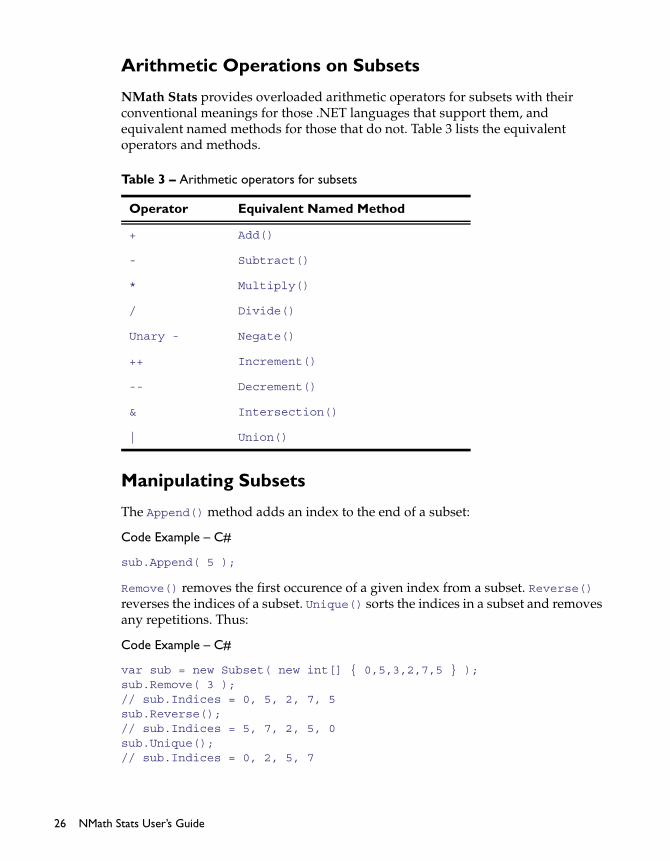
Arithmetic Operations on Subsets
NMath Stats provides overloaded arithmetic operators for subsets with their conventional meanings for those .NET languages that support them, and equivalent named methods for those that do not. Table 3 lists the equivalent operators and methods.
Manipulating Subsets
The Append() method adds an index to the end of a subset:
Code Example – C#
sub.Append( 5 );
Remove() removes the first occurence of a given index from a subset. Reverse() reverses the indices of a subset. Unique() sorts the indices in a subset and removes any repetitions. Thus:
Code Example – C#
var sub = new Subset( new int[] { 0,5,3,2,7,5 } );sub.Remove( 3 );// sub.Indices = 0, 5, 2, 7, 5sub.Reverse();// sub.Indices = 5, 7, 2, 5, 0sub.Unique();// sub.Indices = 0, 2, 5, 7
Table 3 – Arithmetic operators for subsets
Operator Equivalent Named Method
+ Add()
- Subtract()
* Multiply()
/ Divide()
Unary - Negate()
++ Increment()
-- Decrement()
& Intersection()
| Union()
26 NMath Stats User’s Guide
Similarly, ToReverse() returns a new subset containing the indices of a subset in the reverse order; ToUnique() returns a new subset containing the sorted indices of a subset, with all repetitions removed.
The Repeat() method creates a new subset by repeating the source subset until a given length is reached. For instance:
Code Example – C#
var sub1 = new Subset( 3 );// sub1.Indices = 0,1,2Subset sub2 = sub1.Repeat( 11 );// sub2.Indices = 0,1,2,0,1,2,0,1,2,0,1
The Split() method splits a source subset into an arbitrary array of subsets. The parameters are the number of subsets into which to split the source subset, and another subset the same length as the source subset, the ith element of which indicates into which bin to place the ith element of the source subset. For example:
Code Example – C#
var sub = new Subset( 10 );// sub.Indices = 0,1,2,3,4,5,6,7,8,9Subset bins = new Subset( new int[] { 3, 1, 0, 2, 2, 1, 1, 2, 3, 0 } );Subset[] subsetArray = sub.Split( 4, bins );// subsetArray[0] = 2,9// subsetArray[1] = 1,5,6// subsetArray[2] = 3,4,7// subsetArray[3] = 0,8
Lastly, the ToString() returns a comma-delimited string list of the indices in a subset.
Groupings
The static GetGroupings() methods on Subset create subsets from factors. One overload of this method accepts a single Factor and returns an array of subsets containing the indices for each level of the given factor. Another overload accepts two Factor objects and returns a two-dimensional jagged array of subsets containing the indices for each combination of levels in the two factors. See Section 2.10 for more information on factors and the GetGroupings() methods.
Random Samples
The static method Sample( n ) returns a random shuffle of 0..n-1. The returned Subset can be used to randomly reorder the rows in a data frame, as described in Section 2.8.
Chapter 2. Data Frames 27
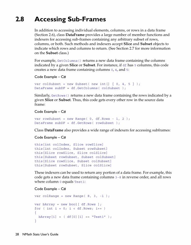
2.8 Accessing Sub-Frames
In addition to accessing individual elements, columns, or rows in a data frame (Section 2.6), class DataFrame provides a large number of member functions and indexers for accessing sub-frames containing any arbitrary subset of rows, columns, or both. Such methods and indexers accept Slice and Subset objects to indicate which rows and columns to return. (See Section 2.7 for more information on the Subset class.)
For example, GetColumns() returns a new data frame containing the columns indicated by a given Slice or Subset. For instance, if df has 5 columns, this code creates a new data frame containing columns 0, 4, and 5:
Code Example – C#
var colSubset = new Subset( new int[] { 0, 4, 5 } );DataFrame subDF = df.GetColumns( colSubset );
Similarly, GetRows() returns a new data frame containing the rows indicated by a given Slice or Subset. Thus, this code gets every other row in the source data frame:
Code Example – C#
var rowSubset = new Range( 0, df.Rows - 1, 2 );DataFrame subDF = df.GetRows( rowSubset );
Class DataFrame also provides a wide range of indexers for accessing subframes:
Code Example – C#
this[int colIndex, Slice rowSlice]this[int colIndex, Subset rowSubset]this[Slice rowSlice, Slice colSlice]this[Subset rowSubset, Subset colSubset]this[Slice rowSlice, Subset colSubset]this[Subset rowSubset, Slice colSlice]
These indexers can be used to return any portion of a data frame. For example, this code gets a new data frame containing columns 3-8 in reverse order, and all rows where column 0 equals Test1:
Code Example – C#
var colRange = new Range( 8, 3, -1 );
var bArray = new bool[ df.Rows ];for ( int i = 0; i < df.Rows; i++ ){ bArray[i] = ( df[0][i] == “Test1” );}
28 NMath Stats User’s Guide

var rowSubset = new Subset( bArray );
DataFrame df2 = df[ rowSubset, colRange ];
Finally, there is the GetSubRow() method. Whereas GetRow() returns an entire row for a given row index, GetSubRow() returns the portion of the row indicated by the given column Slice or Subset:
Code Example – C#
var colSlice = new Slice( 0, 3, 1 );object[] subRow = df.GetSubRow( 3, colSlice );
2.9 Reordering DataFrames
The DataFrame class provides method for both sorting rows, and for arbitrarily reordering rows and columns.
Sorting Rows
The SortRows() method sorts the rows in a data frame according to a given ordered array of column indices. The first index is the primarily sort column, the second index is the secondary sort column, and so forth. For instance:
Code Example – C#
df.SortRows( 3, 0, 1 );
By default, all sorting is in ascending order.
For more control, you can also pass an array of SortingType enumerated values (Ascending or Descending):
Code Example – C#
int[] colIndices = { 3, 0, 1 };SortingType[] sortingTypes = { SortingType.Ascending, SortingType.Descending, SortingType.Ascending };df.SortRows( colIndices, sortingTypes );
Finally, the SortRowsByKeys() method sorts the rows in a data frame by their row keys, in the specified order:
Code Example – C#
df.SortRowsByKeys( SortingType.Ascending );
NOTE—StatsSettings.Sorting specifies the default SortingType.
Chapter 2. Data Frames 29

Permuting Rows and Columns
The PermuteColumns() and PermuteRows() methods enable you to arbitrarily reorder the columns and rows in a data frame, respectively. Each method takes an array of indices. The array must be same length as the number of columns or rows, and contain unique indices. In both cases:
Code Example – C#
new[ permutation[i] ] = old[ i ]
For example, assuming df has 3 columns, this code switches the last two columns:
Code Example – C#
df.PermuteColumns( 0, 2, 1 );
Assuming df has 5 rows, this code moves the second and fourth rows to the top:
Code Example – C#
df.PermuteRows( 2, 0, 3, 1, 4 );
2.10 Factors
The Factor class represents a categorical vector in which all elements are drawn from a finite number of factor levels. Thus, a Factor contains two parts:
an object array of factor levels
an integer array of categorical data, of which each element is an index into the array of levels
For example, this string data:
“A”, “A”, “C”, “B”, “A”, “C”, “B”
could be presented as a Factor with the following levels and categorical data:
Code Example – C#
object[] levels = { “A”, “B”, “C” };int[] data = { 0, 0, 2, 1, 0, 2, 1 };
Factors are usually constructed from a data frame column using the GetFactor() method, but they can also be constructed independently.
30 NMath Stats User’s Guide

Creating Factors
The GetFactor() method on DataFrame accepts a column index or name and returns a Factor with levels for the sorted, unique elements in the given column:
Code Example – C#
Factor myColFactor = df.GetFactor( “myCol” );
Alternatively, you can provide the factor levels yourself. The order is preserved. Thus:
Code Example – C#
var levels = new object[] { “Q1”, “Q2”, “Q3”, “Q4” };Factor myColFactor = df.GetFactor( “myCol”, levels );
An InvalidArgumentException is raised if the specified column contains a value not present in the given array of levels.
You can also construct a Factor independently of a DataFrame. For example, you can construct a Factor from an array of values:
Code Example – C#
var strArray = new object[] { 1, 1, 3, 2, 1, 3, 2 };var factor = new Factor( strArray );
Factor levels are constructed from a sorted list of unique values in the passed array.
Alternatively, you can construct a Factor from an array of factor levels, and a data array consisting of indices into the factor levels:
Code Example – C#
var levels = new object[] { 1, 2, 3 };var data = new int[] { 0, 0, 2, 1, 0, 2, 1 };var factor = new Factor( levels, data );
An InvalidArgumentException is thrown if the given data array contains an invalid index.
Properties of Factors
The Factor class provides the following properties:
Data gets the categorical data for the factor. Each element in the returned integer array is an index into Levels.
Levels gets the levels of the factor as an array of objects.
Length gets the length of the Data in the factor.
Chapter 2. Data Frames 31

Name gets and set the name of the factor.
NumberOfLevels gets the number of levels in the factor.
Accessing Factors
A standard indexer is provided for accessing the element at a given index:
Code Example – C#
string str = (string)factor[2];
The indexer returns Levels[ Data[index] ]—that is, it returns the level at the given position.
Creating Groupings with Factors
The principal use of factors is in conjunction with the GetGroupings() methods on Subset. One overload of this method accepts a single Factor and returns an array of subsets containing the indices for each level of the given factor. Another overload accepts two Factor objects and returns a two-dimensional jagged array of subsets containing the indices for each combination of levels in the two factors.
For example, suppose we weigh human subjects based on sex and age group. The data for 15 subject might look like this:
Table 4 – Sample data
In a DataFrame, each observation would be a row, like so:
Code Example – C#
var df = new DataFrame();df.AddColumn( new DFStringColumn( "Sex" ) ); df.AddColumn( new DFStringColumn( "AgeGroup" ));df.AddColumn( new DFIntColumn( "Weight" ) );
df.AddRow( "John Smith", "Male", "Child", 45 );df.AddRow( "Ruth Barnes", "Female", "Senior", 115 );df.AddRow( "Jane Jones", "Female", "Adult", 115 );df.AddRow( "Timmy Toddler", "Male", "Child", 42 );df.AddRow( "Betsy Young", "Female", "Adult", 130 );
Male Female
Child 45, 42 30, 35, 60, 40
Adult 182, 170 115, 130, 110
Senior 142, 155 115, 123
32 NMath Stats User’s Guide

df.AddRow( "Arthur Smith", "Male", "Senior", 142 );df.AddRow( "Lucy Young", "Female", "Child", 30 );df.AddRow( "Emma Allen", "Female", "Child", 35 );df.AddRow( "Roy Wilkenson", "Male", "Adult", 182 );df.AddRow( "Susan Schwarz", "Female", "Senior", 110 );df.AddRow( "Ming Tao", "Female", "Senior", 123 );df.AddRow( "Johanna Glynn", "Female", "Child", 60 );df.AddRow( "Randall Harvey", "Male", "Adult", 170 );df.AddRow( "Tom Howard", "Male", "Senior", 155 );df.AddRow( "Jennifer Watson", "Female", "Child", 40 );
In this case, we’re using the subjects’ names as row keys.
It is natural to construct factors from the Sex and AgeGroup columns:
Code Example – C#
Factor sex = df.GetFactor( "Sex" );Factor age = df.GetFactor( "AgeGroup" );
We can then use these factors in conjunction with the GetGroupings() methods on Subset to create subsets representing the original rows, columns, and cells in Table 4:
Code Example – C#
Subset[] sexGroups = Subset.GetGroupings( sex );Subset[] ageGroups = Subset.GetGroupings( age );Subset[,] cellGroups = Subset.GetGroupings( sex, age );
These subsets can then be used to operate on the relevant portions of the data frame. For instance, this code prints out row means, column means, and cell means for Table 4:
Code Example – C#
Console.WriteLine( "\nTABLE ROW MEANS" ); for ( int i = 0; i < age.NumberOfLevels; i++ ){ double mean = StatsFunctions.Mean( df[ df.IndexOfColumn( "Weight" ), ageGroups[i] ] ); Console.WriteLine( "Mean for {0} = {1}", age.Levels[i], mean );}
Console.WriteLine( "\nTABLE COLUMN MEANS" ); for ( int i = 0; i < sex.NumberOfLevels; i++ ){ double mean = StatsFunctions.Mean( df[ df.IndexOfColumn( "Weight" ), sexGroups[i] ] ); Console.WriteLine( "Mean for {0} = {1}", sex.Levels[i], mean );}
Chapter 2. Data Frames 33

Console.WriteLine( "\nTABLE CELL MEANS" );for ( int i = 0; i < sex.NumberOfLevels; i++ ){ for ( int j = 0; j < age.NumberOfLevels; j++ ) { double mean = StatsFunctions.Mean( df[ df.IndexOfColumn( "Weight" ), cellGroups[i,j] ] ); Console.WriteLine( "Mean for {0} {1} = {2}", sex.Levels[i], age.Levels[j], mean ); }}
The output is:
TABLE ROW MEANSMean for Adult = 149.25Mean for Child = 42Mean for Senior = 129
TABLE COLUMN MEANSMean for Female = 84.2222222222222Mean for Male = 122.666666666667
TABLE CELL MEANSMean for Female Adult = 122.5Mean for Female Child = 41.25Mean for Female Senior = 116Mean for Male Adult = 176Mean for Male Child = 43.5Mean for Male Senior = 148.5
See also the Tabulate() convenience methods on class DataFrame, as described in Section 2.11.
2.11 Cross-Tabulation
As described in Section 2.10, the DataFrame.GetFactor() method can be used in conjunction with Subset.GetGroupings() to access “cells” of data based on one or two grouping factors. This is such a common operation that class DataFrame also provides the Tabulate() methods as a convenience. This method accepts one or two grouping columns, a data column, and a delegate to apply to each data column subset. The results are returned in a new data frame.
34 NMath Stats User’s Guide

Column Delegates
Overloads of Tabulate() accept static IDFColumn function delegates that return various types. For instance, this code encapsulates the static StatsFunctions.Mean() function in a Func<IDFColumn, double>:
Code Example – C#
Func<IDFColumn, double> mean = new Func<IDFColumn, double>(StatsFunctions.Mean);
Most of the static descriptive statistics functions on class StatsFunctions (Chapter 3) have overloads that accept an IDFColumn and return a double, and so can be encapsulated in this way. A few return integers.
For example, this code encapsulates StatsFunctions.Count(), which returns the number of items in a column, in a Func<IDFColumn, int>:
Code Example – C#
Func<IDFColumn, int> count = new Func<IDFColumn, int>(StatsFunctions.Count);
Applying Column Delegates to Tabulated Data
The following code fills a DataFrame with some sales data:
Code Example – C#
var df = new DataFrame();df.AddColumn( new DFStringColumn( "Product" ) );df.AddColumn( new DFStringColumn("Month") ); df.AddColumn( new DFIntColumn( "Quantity" ) );df.AddColumn( new DFNumericColumn( "Price" ) );df.AddColumn( new DFNumericColumn( "TotalSale" ) );
int rowID = 0;df.AddRow( rowID++, "Squash", "Nov", 40, 1.50, 60.0 );df.AddRow( rowID++, "Carrots", "Nov", 15, 1.20, 18.0 );df.AddRow( rowID++, "Squash", "Nov", 37, 1.45, 53.65 );df.AddRow( rowID++, "Carrots", "Nov", 18, 1.25, 22.50 );df.AddRow( rowID++, "Squash", "Nov", 34, 1.39, 47.26 );df.AddRow( rowID++, "Carrots", "Dec", 20, 1.30, 26.0 );df.AddRow( rowID++, "Squash", "Dec", 31, 1.30, 40.30 );df.AddRow( rowID++, "Carrots", "Dec", 25, 1.40, 35.0 );df.AddRow( rowID++, "Squash", "Dec", 25, 1.25, 31.25 );df.AddRow( rowID++, "Carrots", "Dec", 30, 1.45, 43.50 );df.AddRow( rowID++, "Carrots", "Jan", 33, 1.50, 49.50 );df.AddRow( rowID++, "Squash", "Jan", 19, 1.21, 22.99 );df.AddRow( rowID++, "Carrots", "Jan", 40, 1.65, 66.0 );df.AddRow( rowID++, "Squash", "Jan", 15, 1.11, 16.65 );
Chapter 2. Data Frames 35
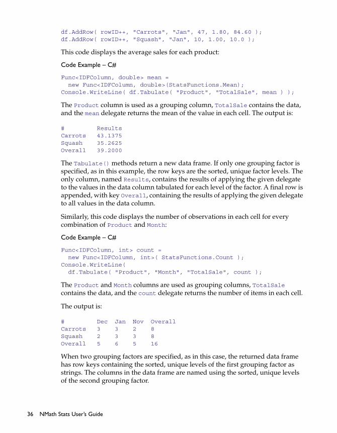
df.AddRow( rowID++, "Carrots", "Jan", 47, 1.80, 84.60 );df.AddRow( rowID++, "Squash", "Jan", 10, 1.00, 10.0 );
This code displays the average sales for each product:
Code Example – C#
Func<IDFColumn, double> mean = new Func<IDFColumn, double>(StatsFunctions.Mean);Console.WriteLine( df.Tabulate( "Product", "TotalSale", mean ) );
The Product column is used as a grouping column, TotalSale contains the data, and the mean delegate returns the mean of the value in each cell. The output is:
# ResultsCarrots 43.1375Squash 35.2625Overall 39.2000
The Tabulate() methods return a new data frame. If only one grouping factor is specified, as in this example, the row keys are the sorted, unique factor levels. The only column, named Results, contains the results of applying the given delegate to the values in the data column tabulated for each level of the factor. A final row is appended, with key Overall, containing the results of applying the given delegate to all values in the data column.
Similarly, this code displays the number of observations in each cell for every combination of Product and Month:
Code Example – C#
Func<IDFColumn, int> count = new Func<IDFColumn, int>( StatsFunctions.Count );Console.WriteLine( df.Tabulate( "Product", "Month", "TotalSale", count );
The Product and Month columns are used as grouping columns, TotalSale contains the data, and the count delegate returns the number of items in each cell.
The output is:
# Dec Jan Nov OverallCarrots 3 3 2 8Squash 2 3 3 8Overall 5 6 5 16
When two grouping factors are specified, as in this case, the returned data frame has row keys containing the sorted, unique levels of the first grouping factor as strings. The columns in the data frame are named using the sorted, unique levels of the second grouping factor.
36 NMath Stats User’s Guide
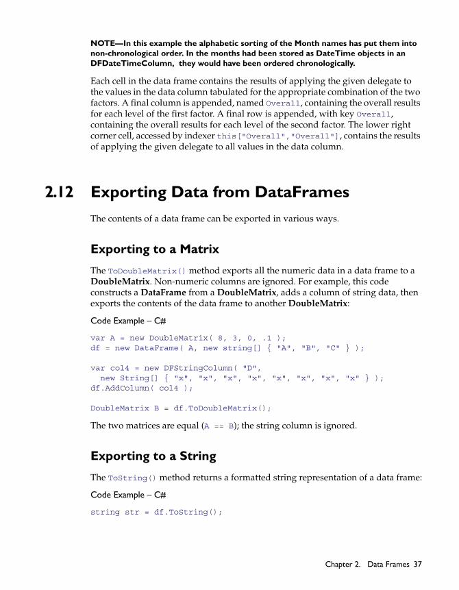
NOTE—In this example the alphabetic sorting of the Month names has put them into non-chronological order. In the months had been stored as DateTime objects in an DFDateTimeColumn, they would have been ordered chronologically.
Each cell in the data frame contains the results of applying the given delegate to the values in the data column tabulated for the appropriate combination of the two factors. A final column is appended, named Overall, containing the overall results for each level of the first factor. A final row is appended, with key Overall, containing the overall results for each level of the second factor. The lower right corner cell, accessed by indexer this["Overall","Overall"], contains the results of applying the given delegate to all values in the data column.
2.12 Exporting Data from DataFrames
The contents of a data frame can be exported in various ways.
Exporting to a Matrix
The ToDoubleMatrix() method exports all the numeric data in a data frame to a DoubleMatrix. Non-numeric columns are ignored. For example, this code constructs a DataFrame from a DoubleMatrix, adds a column of string data, then exports the contents of the data frame to another DoubleMatrix:
Code Example – C#
var A = new DoubleMatrix( 8, 3, 0, .1 );df = new DataFrame( A, new string[] { "A", "B", "C" } );
var col4 = new DFStringColumn( "D", new String[] { "x", "x", "x", "x", "x", "x", "x", "x" } );df.AddColumn( col4 );
DoubleMatrix B = df.ToDoubleMatrix();
The two matrices are equal (A == B); the string column is ignored.
Exporting to a String
The ToString() method returns a formatted string representation of a data frame:
Code Example – C#
string str = df.ToString();
Chapter 2. Data Frames 37

For more control, you can also indicate:
whether to export column headers (the default is true)
whether to export row keys (the default is true)
the delimiter to use to separate columns (the default is tab-delimited)
For instance, this code exports the column headers, but not the row keys, and uses a comma delimiter:
Code Example – C#
string str = df.ToString( true, false, “,” );
Convenience methods are also provided for persisting a text representation of a data frame to a text file. Save() exports the contents of the data frame to a given filename:
Code Example – C#
df.Save( “myData.txt” );
Again, you can also indicate whether to export column header or row keys, and specify the column delimiter:
Code Example – C#
df.Save( “myData.txt”, true, false, “,” );
The LaunchSaveFileDialog() method allows the end user to specify the filename. The OpenInEditor() method programmatically opens a data frame in the default text editor on the user’s system. The user can then edit the contents of the data frame. Lastly, the static Load() method imports a data frame from a text file:
Code Example – C#
DataFrame df = DataFrame.Load( “myData.txt” );
Again, you can indicate whether the text file includes column headers and row keys, and the delimiter used to separate the columns.
38 NMath Stats User’s Guide
Exporting to an ADO.NET DataTable
The ToDataTable() method exports the data in a data frame to an ADO.NET DataTable object. The row keys are placed in a DataColumn named DFRowKeys. Thus, this code:
Code Example – C#
var df = new DataFrame();df.AddColumn( new DFNumericColumn( "ids", new DoubleVector( 3, 3, -1 )));df.AddColumn( new DFStringColumn( "names", "a", "b", "c" ));df.AddColumn( new DFBoolColumn( "bools", true, false, true ));df.SetRowKeys( new String[] { "Row1", "Row2", "Row3" } );DataTable table = df.ToDataTable();
returns a DataTable that looks like this:
name: CenterSpace.NMath.Stats.DataFrame# DFRowKeys ids names bools1 Row1 3.0000 a True2 Row2 2.0000 b False3 Row3 1.0000 c True
If no name is assigned to a data frame before ToDataTable() is called, the name of the DataTable is set to the type: CenterSpace.NMath.Stats.DataFrame.
Binary and SOAP Serialization
Class DataFrame implements the ISerializable interface to control serialization and deserialization. Common Language Runtime (CLR) serialization Formatter classes call the provided GetObjectData() method at serialization time to populate a SerializationInfo object with all the data required to represent a DataFrame. For example, the BinaryFormatter class provides Serialize() and Deserialize() methods for persisting an object in binary format to a given stream. For example, this code serializes a data frame to a file:
Code Example – C#
using System.IO;using System.Runtime.Serialization.Formatters.Binary;
FileStream binStream = File.Create( “myData.dat” );var binFormatter = new BinaryFormatter();binFormatter.Serialize( binStream, df );binStream.Close();
Chapter 2. Data Frames 39
This code restores the data frame from the file:
Code Example – C#
binStream = File.OpenRead( "myData.dat" );DataFrame df2 = (DataFrame)binFormatter.Deserialize( binStream );binStream.Close();File.Delete( "myData.dat" );
Similarly, the SoapFormatter class persists an object in SOAP format to a given stream. Thus:
Code Example – C#
using System.IO;using System.Runtime.Serialization.Formatters.Soap;
FileStream xmlStream = File.Create( "myData.xml" );var xmlFormatter = new SoapFormatter();xmlFormatter.Serialize( xmlStream, df );xmlStream.Close();
This code restores the data frame from the file:
Code Example – C#
xmlStream = File.OpenRead( "myData.xml" );DataFrame df2 = (DataFrame)xmlFormatter.Deserialize( xmlStream )xmlStream.Close();File.Delete( "myData.xml" );
40 NMath Stats User’s Guide

CHAPTER 3. DESCRIPTIVE STATISTICS
Class StatsFunctions provides a wide variety of static functions for computing descriptive statistics, such as mean, variance, standard deviation, percentile, median, quartiles, geometric mean, harmonic mean, RMS, kurtosis, skewness, and many more.
Method overloads accept data as an array of doubles, as a DoubleVector, or as a column in a DataFrame (Chapter 2). For example:
Code Example – C#
double[] dblArray = { 1.12, -2.0, 3.88, 1.2, 15.345 };double mean1 = StatsFunctions.Mean( dblArray );
var v = new DoubleVector( “1.12 -2.0 3.88 1.2 15.345” );double mean2 = StatsFunctions.Mean( v );
var df = new DataFrame();df.AddColumn( new DFNumericColumn( "myData", 1.12, -2.0, 3.88, 1.2, 15.345 ) );double mean3 = StatsFunctions.Mean( df[ “myData” ] );
// mean1 == mean2 == mean3
In this chapter, where data is used in code examples, it should be understood to be an instance of any of these three types.
3.1 Column Types
Most functions in class StatsFunctions require numeric data, although they accept any instance of IDFColumn. If a column is not an instance of DFIntColumn or DFNumericColumn, an attempt is made to convert the data to double using System.Convert.ToDouble().
NOTE—An NMathFormatException is raised if the data cannot be converted to double.
Chapter 3. Descriptive Statistics 41

For instance, these functions will work with a DFStringColumn containing numbers represented as strings.
Code Example – C#
DFStringColumn col = new DFStringColumn( “Col1”, “1.5”, “2”, “1.33”, “4.76” );double mean = StatsFunctions.Mean( col );;
However, there is a processing penalty due to such type conversion. If you need to perform many statistical functions on a column, first create a new DFIntColumn or DFNumericColumn from your data column, so type conversion occurs only once. For example, if column 4 in data frame df is a DFGenericColumn containing decimal types, this works:
Code Example – C#
double mean = StatsFunctions.Mean( df[4] );double stdev = StatsFunctions.StandardDeviation( df[4] );
but the decimal data is converted to doubles twice. This code first creates a new DFNumericColumn containing doubles from the generic column, then computes the statistics:
Code Example – C#
var col = new DFNumericColumn( df[4].Name, df[4] );double mean = StatsFunctions.Mean( col );double stdev = StatsFunctions.StandardDeviation( col );
In some cases, you may want to replace the original generic column in the data frame with the new DFNumericColumn:
Code Example – C#
df.RemoveColumn( 4 );df.InsertColumn( 4, col );double mean = StatsFunctions.Mean( df[4] );double stdev = StatsFunctions.StandardDeviation( df[4] );
Note that sometimes you may not even be aware that your data is stored in a generic column. (You can always return the type of a column using the ColumnType property.) This is most likely to occur when you read data from a text file or database directly into a DataFrame. For example, if your database stores data using SQL NUMERIC or DECIMAL types, these get mapped to System.Decimal in ADO. NMath does not silently convert decimals to doubles, because of the loss of precision, so they are stored in the dataframe as objects in a DFGenericColumn. If you intend to perform multiple statistical functions on the data, convert the column to a DFNumericColumn first, as shown above.
42 NMath Stats User’s Guide
3.2 Missing Values
Most functions in class StatsFunctions are accompanied by a paired function that ignores missing values, such as Double.NaN in a DoubleVector, DFNumericColumn, or array of doubles. For example, there are Mean() and NaNMean() functions, Variance() and NaNVariance() functions, and so forth. Unless a function is explicitly designed to handle missing values, it may return NaN or have unexpected results if values are missing.
Code Example – C#
DoubleVector v = new DoubleVector( “[ 3.2 1.0 Double.NaN 4.5 -1.2 ]”);
double mean1 = StatsFunctions.Mean( v );// mean1 = Double.NaN
double mean2 = StatsFunctions.NaNMean( v );// mean2 = 1.875
The provided convenience method NaNCheck() returns true if a given data set contains any missing values. NaNRemove() creates a copy of a data set with missing values removed. For two-dimensional data sets, such as matrices and data frames, NaNRemoveCols() creates a copy with only those columns that do not contain missing values. NaNRemoveRows() removes any rows containing missing data. The CleanCols() and CleanRows() methods on class DataFrame have the same effect.
As described in Section 2.1, data frame column types enable you to specify how missing values are represented within a particular column instance, or for all columns of a particular type. For example, this column stores numeric data in a string column, and uses NA to indicate a missing value:
Code Example – C#
DFStringColumn col = new DFStringColumn( “myCol”, “32.1”, “NA”, “6.0”, “34” );
This code identifies the missing value string, then computes the mean, ignoring missing values:
Code Example – C#
col.MissingValue = “NA”;double mean = StatsFunctions.NaNMean( col );
Because the column is not an instance of DFIntColumn or DFNumericColumn, an attempt is made to convert the data to double using System.Convert.ToDouble() (Section 3.1). If StatsFunctions.Mean() was used, instead of
Chapter 3. Descriptive Statistics 43

StatsFunctions.NaNMean(), or if col.MissingValue was set to something other than NA (for example, the default value is “.”), an exception would be thrown.
3.3 Counts and Sums
The static Count() method on class StatsFunctions returns the number of elements in a data set:
Code Example – C#
int numElements = StatsFunctions.Count( data );
Counts() returns an IDictionary of key-value pairs in which the keys are the unique elements in a given data set, and the values are the counts for each element.
CountIf() calculates how many elements in a data set return true when a logical function is applied. For example, suppose MeetsThreshold() is a method that returns true if a given numeric value is greater than 100:
Code Example – C#
public bool MeetsThreshold( double x ){ return ( x > 100 );}
This code counts the number of elements in a data set that meet the criterion:
Code Example – C#
int num = StatsFunctions.CountIf( data, new new Func<double, bool>( MeetsThreshold ) );
Similarly, the static Sum() method sums the elements in a data set. SumIf() sums the elements in a data set that return true when a logical function is applied:
Code Example – C#
double sum = StatsFunctions.SumIf( data, new new Func<double, bool>( MeetsThreshold ) );
An overload of SumIf() sums the elements in one data set based on evaluating a logical function on another data set. For instance, this code sums the elements in data2 that correspond to those elements in data where MeetsThreshold() returns true:
Code Example – C#
double sum = StatsFunctions.SumIf( data, function, data2 );
44 NMath Stats User’s Guide

A MismatchedSizeException is raised if the two data sets do not have the same number of elements.
3.4 Min/Max Functions
Class StatsFunctions provides static min/max finding methods that return the integer index of the element in a data set that meets the appropriate criterion:
MaxIndex() returns the index of the element with the greatest value.
MinIndex() returns the index of the element with the smallest value.
MaxAbsIndex() returns the index of the element with the greatest absolute value.
MinAbsIndex() returns the index of the element with the smallest absolute value.
Min/max value methods MaxValue(), MinValue(), MaxAbsValue(), and MinAbsValue() return the value of the element that meets the appropriate criterion.
3.5 Ranks, Percentiles, Deciles, and Quartiles
The static Ranks() method on class StatsFunctions returns the rank of each element in a data set an as array of integers. For example:
Code Example – C#
int[] ranks = StatsFunctions.Ranks( data );
By default, the ranks are calculated using ascending order. Alternatively, you can specify a sort order using a value from the SortingType enumeration. Thus:
Code Example – C#
int[] ranks = StatsFunctions.Ranks( data, SortingType.Descending );
NOTE—StatsSettings.Sorting specifies the default SortingType.
The Rank() method returns where a given value would rank within a data set, if it were part of the data set. Again, the sorting order can be specified using a value from the SortingType enumeration. For instance:
Chapter 3. Descriptive Statistics 45

Code Example – C#
double x = 5.342;int rank = StatsFunctions.Rank( data, x, SortingType.Descending );
Percentile() calculates the value at the nth percentile of the elements in a data set, where . For example, to find the value at the 95th percentile:
Code Example – C#
double x = StatsFunctions.Percentile( data, 0.95 );
PercentileRank() performs the inverse calculation, returning the percentile a given value would have if it were part of the data set:
Code Example – C#
double x = 23.653;double percentile = StatsFunctions.Percentile( data, x );
The returned percentile value is between 0 and 1.
Similarly, Decile() calculates a given decile, specified as an integer between 0 and 10, of the elements in a data set. Quartile() calculates a given quartile, specified as an integer between 0 and 4. For example, this code finds the third quartile value:
Code Example – C#
double x = StatsFunctions.Quartile( data, 3 );
3.6 Central Tendency
Measures of central tendency are measures of the location of the middle or the center of a data set. For example, the static Mean() method on class StatsFunctions computes the arithmetic mean (average) of the elements in a data set:
Code Example – C#
double mean = StatsFunctions.Mean( data );
Median() calculates the median of the elements in a data set:
Code Example – C#
double median = StatsFunctions.Median( data );
The median is the middle of the set—half the values are above the median and half are below the median. If there are an even number of elements, Median() returns the average of the middle two elements.
Mode() determines the most frequently occurring value in a data set:
0 n 1
46 NMath Stats User’s Guide

Code Example – C#
double mode = StatsFunctions.Mode( data );
GeometricMean() calculates the geometric mean.
HarmonicMean() calculates the harmonic mean.
TrimmedMean() calculates the mean of a data set after the specified trimming. A trimmed mean is calculated by discarding a certain percentage of the lowest and the highest values and then computing the mean of the remaining values. For example, a mean trimmed 50% is computed by discarding the lower and higher 25% of the values and taking the mean of the remaining values. TrimmedMean() takes a trimming parameter, which is a value between 0.0 and 1.0. For example, this code computes the mean trimmed 50%:
Code Example – C#
double trimMean = StatsFunctions.TrimmedMean( data, 0.50 );
The median is the mean trimmed 1.0, and the arithmetic mean is the mean trimmed 0.0.
WeightedMean() calculates the weighted average of all the elements in a data set using a given set of corresponding weights. The weighted mean is calculated as
For instance:
Code Example – C#
var v = new DoubleVector( "-0.3 -0.03 4 2.8 -12.3 -5 3 10" );var weights = new DoubleVector( "1 2 3 4 2 1 3 4" );double weightedMean = StatsFunctions.WeightedMean( v, weights ))
A MismatchedSizeException is raised if the number of weights does not equal the number of elements in the data set. Note that if all the weights are equal, the weighted mean is the same as the arithmetic mean.
n
x1 x1xnn
------------------------------
n
1x1---- 1
x2---- 1
xn----+ + +
----------------------------------------
w1x1 w2x2 wnxn+ + +
w1 w2 wn+ + +----------------------------------------------------------
Chapter 3. Descriptive Statistics 47

Lastly, RMS() calculates the root mean square of the elements in a data set. RMS, sometimes called the quadratic mean, is the square root of the mean squared value.
3.7 Spread
Measures of spread are measures of the degree values in the data set differ from each other. For example, the static SumOfSquaredErrors() method on class StatsFunctions calculates the sum of squared errors (SSE) of the elements in the data set. SSE is the sum of the squared differences between each element and the mean.
StandardDeviation() computes the biased standard deviation of the elements in a data set.
For instance:
Code Example – C#
double stdev = StatsFunctions.StandardDeviation( data );
Alternatively, you can specify the unbiased standard deviation
using a value from the BiasType enumeration:
Code Example – C#
double stdev = StatsFunctions.StandardDeviation( data, BiasType.Unbiased );
NOTE—StatsSettings.Bias specifies the default BiasType.
Variance() calculates the variance of the elements in a data set. Variance is the square of the standard deviation. Again, you can specify a biased or unbiased estimator using values from the BiasType enumeration.
MeanDeviation() calculates the mean deviation of the elements in a data set. The mean deviation is the mean of the absolute deviations about the mean. The mean deviation is defined by
SSEn
-----------
SSEn 1–-----------
1n--- xi x–
i 1=
n
48 NMath Stats User’s Guide

Similarly, MedianDeviationFromMean() calculates the median of the absolute deviations from the mean. MedianDeviationFromMedian() calculates the median of the absolute deviations from the median.
Lastly, InterquartileRange() returns the difference between the median of the highest half and the median of the lowest half of the elements in a data set:
Code Example – C#
double iqr = StatsFunctions.InterQuartileRange( data );
3.8 Shape
The static Skewness() method on class StatsFunctions computes the skewness of the elements in a data set. Skewness is the degree of asymmetry of a distribution. A distribution is skewed if one of its tails is longer than the other. Thus:
Code Example – C#
double skewness = StatsFunctions.Skewness( data );
By default, Skewness() uses a biased estimator of the standard deviation (Section 3.7). Alternatively, you can specify the unbiased standard deviation using a value from the BiasType enumeration:
Code Example – C#
double skewness = StatsFunctions.Skewness( data, BiasType.Unbiased );
NOTE—StatsSettings.Bias specifies the default BiasType.
Kurtosis() calculates the kurtosis of the elements in a data set. Kurtosis is a measure of the degree of peakedness of a distribution. Again, a biased estimator of the standard deviation is used by default—you can specify the unbiased standard deviation using a value from the BiasType enumeration.
Finally, CentralMoment() returns the moment about the mean of a data set specified by a positive integer order. The first central moment is equal to zero. The second central moment is the variance. The third central moment is the skewness. The fourth central moment is the kurtosis.
Chapter 3. Descriptive Statistics 49
3.9 Covariance, Correlation, and Autocorrelation
The static Covariance() method on class StatsFunctions computes the covariance of two data sets. Covariance is a measure of the tendency of two data sets to vary together, and is defined by
Each deviation score in the first data set is multiplied by the corresponding deviation score in the second data set. For example:
Code Example – C#
double cov = StatsFunctions.Covariance( data1, data2 );
You can also specify a biased or unbiased estimator using values from the BiasType enumeration.
CovarianceMatrix() creates a square, symmetric matrix containing the variances and covariances of the columns in a given data matrix. The diagonal elements represent the variances for the columns; the off-diagonal elements represent the covariances of each pair of columns.
Correlation() calculates the correlation between two data sets. Correlation is covariance standardized by dividing by the standard deviation of each data set:
The resultant value is the Pearson product-moment correlation coefficient, more commonly known simply as the correlation.
Spearmans() calculates the Spearman rank correlation coefficient, commonly known as Spearman’s rho. Spearman’s rho differs from Pearson's correlation only in that the computation is done after the values in the data set are converted to ranks (Section 3.5).
Fisher() calculates the Fisher transformation at a given value, which can be used to perform hypothesis testing on the correlation coefficient. FisherInv() calculates the inverse Fisher transformation.
Cronbach() calculates the standardized Cronbach’s alpha test for reliability.
Autocorrelation is the correlation between members of a time series of observations. Class StatsFunctions provides two static methods for computing first-order autocorrelation:
covx y
xi x– yi y– n
--------------------------------------------=
corx ycovx ySxSy
---------------=
50 NMath Stats User’s Guide

DurbinWatson() calculates the Durbin-Watson statistic for the elements in a data set.
VonNeumannRatio() calculates the Von Neumann ratio for the elements in a data set.
For instance:
Code Example – C#
double dw = StatsFunctions.DurbinWatson( data );double vnr = StatsFunctions.VonNeumannRatio( data );
3.10 Sorting
The static Sort() method on class StatsFunctions sorts the elements of a data set in ascending or descending order using the quicksort algorithm and returns a new data set containing the result. The sort order is specified using a value from the SortingType enumeration.
For example:
Code Example – C#
var v = new DoubleVector( “5 7 1 3 9 4 5 2 1 0 11 3” ); v = StatsFunctions.Sort( v, SortingType.Descending );
NOTE—StatsSettings.Sorting specifies the default SortingType.
3.11 Logical Functions
The static If() method on class StatsFunctions creates an array of boolean values determined by applying a given logical function to the elements in a data set.
For example, suppose OnInterval01() is a method that returns true if a given numeric value is between 0 and 1:
Code Example – C#
public bool OnInterval01( double x ){ return ( ( x >= 0 ) && ( x <= 1 ) );}
Chapter 3. Descriptive Statistics 51

This code creates an array of boolean values by applying the criterion to a data set:
Code Example – C#
bool[] bArray = StatsFunctions.If( data, new new Func<double, bool>( OnInterval01 ) );
As described in Section 2.7, the resultant boolean array could be used to create a Subset containing the indices of all true elements in the array. The subset could then be used to create a sub-frame from a DataFrame containing the rows or columns than meet the criterion.
An overload of If() creates a new data set by applying a logical function to the elements of another data set. Elements in the original data set that return true are set to a given true value in the new data set; elements that return false are not changed.
For instance, suppose GreaterThan100() is a method that returns true if a given numeric value is greater than 100. This code creates a new data in which all values in DoubleVector data that are greater than 100 are set to NaN:
Code Example – C#
DoubleVector data2 = StatsFunctions.If( data, new Func<double, bool>( GreaterThan100 ), Double.NaN );
You can also supply a false value, in which case elements in the original data set that return false are set to that value.
Static CountIf() and SumIf() methods are also provided on class StatsFunctions. See Section 3.3 for more information.
52 NMath Stats User’s Guide

CHAPTER 4. PROBABILITY DISTRIBUTIONS
NMath Stats provides classes for computing the probability density function (PDF), the cumulative distribution function (CDF), the inverse cumulative distribution function, and random variable moments for a variety of probability distributions, including beta, binomial, chi-square ( ), exponential, F, gamma, geometric, Johnson, logistic, log-normal, negative binomial, normal (Gaussian), Poisson, Student's t, triangular, uniform, and Weibull distributions. The distribution classes share a common interface, so once you learn how to use one distribution class, it’s easy to use any of the others.
This chapter describes the distribution classes and how to use them. This chapter also describes how to create correlated sets of random variables drawn from different distributions.
4.1 Distribution Classes
The NMath Stats probability distribution classes are listed in Table 5.
Table 5 – Probability Distribution Classes
Class Distribution
BetaDistribution Beta distribution
BinomialDistribution Binomial distribution
ChiSquareDistribution Chi-Square ( ) distribution
ExponentialDistribution Exponential distribution
FDistribution F distribution
GammaDistribution Gamma distribution
GeometricDistribution Geometric distribution
2
2
Chapter 4. Probability Distributions 53
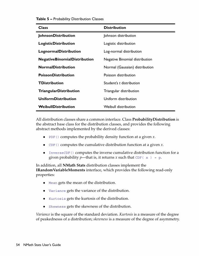
All distribution classes share a common interface. Class ProbabilityDistribution is the abstract base class for the distribution classes, and provides the following abstract methods implemented by the derived classes:
PDF() computes the probability density function at a given x.
CDF() computes the cumulative distribution function at a given x.
InverseCDF() computes the inverse cumulative distribution function for a given probability p—that is, it returns x such that CDF( x ) = p.
In addition, all NMath Stats distribution classes implement the IRandomVariableMoments interface, which provides the following read-only properties:
Mean gets the mean of the distribution.
Variance gets the variance of the distribution.
Kurtosis gets the kurtosis of the distribution.
Skewness gets the skewness of the distribution.
Variance is the square of the standard deviation. Kurtosis is a measure of the degree of peakednesss of a distribution; skewness is a measure of the degree of asymmetry.
JohnsonDistribution Johnson distribution
LogisticDistribution Logistic distribution
LognormalDistribution Log-normal distribution
NegativeBinomialDistribution Negative Binomial distribution
NormalDistribution Normal (Gaussian) distribution
PoissonDistribution Poisson distribution
TDistribution Student’s t distribution
TriangularDistribution Triangular distribution
UniformDistribution Uniform distribution
WeibullDistribution Weibull distribution
Table 5 – Probability Distribution Classes
Class Distribution
54 NMath Stats User’s Guide

Once you have constructed a derived distribution type, you can query it for the PDF, CDF, inverse CDF, and random variable moments. For example, this code constructs a NormalDistribution with mean 0 and variance 1, then queries it:
Code Example – C# normal distribution
var dist = new NormalDistribution( 0, 1 );double pdf = dist.PDF( 0 );double cdf = dist.CDF( 0 );double invCdf = dist.InverseCDF( .5 );double mean = dist.Mean;double var = dist.Variance;double kurt = dist.Kurtosis;double skew = dist.Skewness;
Beta Distribution
Class BetaDistribution represents the beta probability distribution. The beta distribution is a family of curves with two free parameters, usually labelled and
. Beta distributions are nonzero only on the interval (0 1).
The distribution function for the beta distribution is:
where is the beta function. The beta CDF is the same as the incomplete beta function.
For example, this code constructs a BetaDistribution:
Code Example – C# beta distribution
double alpha = 3;double beta = 7;var dist = new BetaDistribution( alpha, beta );
The default constructor creates a BetaDistribution with and equal to 1:
Code Example – C# beta distribution
var dist = new BetaDistribution();
The provided Alpha and Beta properties can be used to get and set the shape parameters after construction:
Code Example – C# beta distribution
dist.Alpha = 4;dist.Beta = 10;
f x x 1–
1 x– 1–
B , ---------------------------------------=
B x y,
Chapter 4. Probability Distributions 55

Once you have constructed a BetaDistribution object, you can query it for the PDF, CDF, inverse CDF, and random variable moments, as described in Section 4.1.
Binomial Distribution
Class BinomialDistribution represents the discrete probability distribution of obtaining exactly n successes in N trials where the probability of success on each trial is p. For example, this code constructs an BinomialDistribution:
Code Example – C# binomial distribution
int n = 20;double p = 0.25;var bin = new BinomialDistribution( n, p );
The default constructor creates an BinomialDistribution with and :
Code Example – C# binomial distribution
var bin = new BinomialDistribution();
The provided N and P properties can be used to get and set the number of trials and the probability of success on each trial after construction:
Code Example – C# binomial distribution
bin.N = 75;bin.P = 0.02;
Once you have constructed an BinomialDistribution object, you can query it for the PDF, CDF, inverse CDF, and random variable moments, as described in Section 4.1.
Chi-Square Distribution
Class ChiSquareDistribution represents the chi-square ( ) probability distribution. The chi-square distribution is a special case of the gamma distribution with and , where df is the degrees of freedom.
For example, this code constructs a ChiSquareDistribution:
Code Example – C# chi-square distribution
double df = 16;var chiSq = new ChiSquareDistribution( df );
n 2= p 0.5=
2
df 2= 2=
56 NMath Stats User’s Guide
The default constructor creates a ChiSquareDistribution with 1 degree of freedom:
Code Example – C# chi-square distribution
var chiSq = new ChiSquareDistribution();
The provided DegreesOfFreedom property can be used to get and set the degrees of freedom of the distribution after construction:
Code Example – C# chi-square distribution
chiSq.DegreesOfFreedom = 10;
Once you have constructed a ChiSquareDistribution object, you can query it for the PDF, CDF, inverse CDF, and random variable moments, as described in Section 4.1.
Exponential Distribution
Class ExponentialDistribution represents the exponential distribution. A random variable w is said to have an exponential distribution if it has a probability density function
where is often called the rate parameter. The mean of an exponential distribution is , and the variance is . For example, this code constructs an ExponentialDistribution:
Code Example – C# exponential distribution
double lambda = 22;ExponentialDistribution exp = new ExponentialDistribution( lambda );
The provided Lambda property can be used to get and set the rate after construction:
Code Example – C# exponential distribution
exp.Lambda = 15;
Once you have constructed an ExponentialDistribution object, you can query it for the PDF, CDF, inverse CDF, and random variable moments, as described in Section 4.1.
g w ew–
=
01 1 2
Chapter 4. Probability Distributions 57

F Distribution
Class FDistribution represents the F probability distribution. The F distribution is the ratio of two chi-square distributions with degrees of freedom df1 and df2, respectively, where each chi-square has first been divided by its degrees of freedom. For example, this code constructs an FDistribution:
Code Example – C# F distribution
double df1 = 11;double df2 = 19;var f = new FDistribution( df1, df2 );
The default constructor creates an FDistribution with both degrees of freedom equal to 1:
Code Example – C# F distribution
var f = new FDistribution();
The provided DegreesOfFreedom1 and DegreesOfFreedom2 properties can be used to get and set the degrees of freedom after construction:
Code Example – C# F distribution
f.DegreesOfFreedom1 = 15;f.DegreesOfFreedom2 = 23;
Once you have constructed an FDistribution object, you can query it for the PDF, CDF, inverse CDF, and random variable moments, as described in Section 4.1.
Gamma Distribution
Class GammaDistribution represents the gamma probability distribution. The gamma distribution is a family of curves with two free parameters, usually labelled and . The mean of the distribution is ; the variance is . When is large, the gamma distribution closely approximates a normal distribution.
The distribution function for the gamma distribution is:
where is the Gamma function.
For example, this code constructs a GammaDistribution:
Code Example – C# gamma distribution
double alpha = 7;double beta = 12;
2
f x x 1–
e
x–------
--------------------=
x
58 NMath Stats User’s Guide
var gamma = new GammaDistribution( alpha, beta );
The default constructor creates a GammaDistribution with and equal to 1:
Code Example – C# gamma distribution
var gamma = new GammaDistribution();
The provided Alpha and Beta properties can be used to get and set the shape parameters after construction:
Code Example – C# gamma distribution
gamma.Alpha = 10;gamma.Beta = 15;
Once you have constructed a GammaDistribution object, you can query it for the PDF, CDF, inverse CDF, and random variable moments, as described in Section 4.1.
Geometric Distribution
Class GeometricDistribution represents the geometric distribution. The geometric distribution is the probability distribution of the number of failures before the first success. It is supported on the set .
A GeometricDistribution is constructed from a given probability of success p, where . For example:
Code Example – C# geometric distribution
double p = .25;var geo = new GeometricDistribution( p );
Class GeometricDistribution provides property P that gets and sets the probability for success for the distribution.
Code Example – C# geometric distribution
geo.P = .5;
Once you have constructed a GeometricDistribution object, you can query it for the PDF, CDF, inverse CDF, and random variable moments, as described in Section 4.1.
Johnson Distribution
Class JohnsonDistribution represents the Johnson system of distributions. The Johnson system is based on three possible transformations of a normal random variable—exponential, logistic, and hyperbolic sine—plus the identity transformation:
0 1 2 3
0 p 1
Chapter 4. Probability Distributions 59

where the transformation f() has four possible forms based on the distribution type:
Normal (SN): f(u) = exp(u)
Log Normal (SL): f(u) = u
Unbounded (SU):f(u) = u + sqrt(1+u^2)
Bounded (SB):f(u) = u/(1-u)
A JohnsonDistribution instance is constructed from a set of distribution parameter values, and a JohnsonTransformationType enumerated value specifying the transformation type. For instance:
Code Example – C# Johnson distribution
double gamma = -0.18;double delta = 2.55;double xi = -0.14;double lambda = 2.35;JohnsonTransformationType type = JohnsonTransformationType.Normal;
JohnsonDistribution dist = new JohnsonDistribution( gamma, delta, xi, lambda, type );
Once you have constructed a JohnsonDistribution object, you can query it for the PDF, CDF, inverse CDF, and random variable moments, as described in Section 4.1.
Class JohnsonDistribution also provides a static Fit() method for fitting a Johnson distribution to a data set. Estimation of the Johnson parameters is done from quantiles that correspond to the cumulative probabilities [0.05, 0.206, 0.5, 0.794, 0.95] using the method of Wheeler (1980).1 For example:
1Wheeler, R.E. (1980). Quantile estimators of Johnson curve parameters. Biometrika. 67-3 725-728.
z ln f u where u+x –
----------- = =
60 NMath Stats User’s Guide

Code Example – C# Johnson distribution
var data = new DoubleVector(-0.09736927, 0.21615254, 0.88246516, 0.20559750, -0.61643584, -0.73479925, -0.13180279, 0.31001699, -1.03968035, -0.18430887, 0.96726726, -0.10828009, - 0.69842067, -0.27594517, 1.11464855, 0.55004396, 1.23667580, 0.13909786, 0.41027510, -0.55845691);var dist = JohnsonDistribution.Fit(data);
The Transform() method transforms data using a JohnsonDistribution object.
Logistic Distribution
Class LogisticDistribution represents the logistic probability distribution with a specified location (mean) and scale. The logistic distribution with location m and scale b has distribution function:
and density:
For example, this code constructs a LogisticDistribution:
Code Example – C# logistic distribution
double loc = 2.0;double scale = 1.5;LogisticDistribution logistic = new LogisticDistribution( loc, scale );
The provided Location and Scale properties can be used to get and set distribution parameters after construction:
Code Example – C# logistic distribution
logistic.Location = 7.123;logistic.Scale = 4.5;
Once you have constructed a LogisticDistribution object, you can query it for the PDF, CDF, inverse CDF, and random variable moments, as described in Section 4.1.
f x 1
1 ex m– – b
+---------------------------------=
f x ex m– – b
b 1 ex m– – b
+ 2
--------------------------------------------=
Chapter 4. Probability Distributions 61

Log-Normal Distribution
Class LognormalDistribution represents the log-normal distribution. A log-normal distribution has a normal distribution as its logarithm:
For example, this code constructs an LognormalDistribution whose associated normal distribution has the specified mean and standard deviation:
Code Example – C# log-normal distribution
double mu = -99;double sigma = 6;var ln = new LognormalDistribution( mu, sigma );
The default constructor creates a LognormalDistribution whose associated normal distribution has mean 0 and standard deviation 1:
Code Example – C# log-normal distribution
var ln = new LognormalDistribution();
The Mu and Sigma properties can be used to get and set the mean and standard deviation after construction:
Code Example – C# log-normal distribution
ln.Mu = 2.25;ln.Sigma = .75;
Once you have constructed a LognormalDistribution object, you can query it for the PDF, CDF, inverse CDF, and random variable moments, as described in Section 4.1.
Negative Binomial Distribution
Class NegativeBinomialDistribution represents the discrete probability distribution of obtaining N successes in a series of x trials, where the probability of success on each trial is P.
For example, this code constructs an NegativeBinomialDistribution:
Code Example – C# negative binomial distribution
int n = 5;double p = 0.25;var negBin = new NegativeBinomialDistribution( n, p );
The default constructor creates an NegativeBinomialDistribution with and :
f x enormal
=
n 2=p 0.5=
62 NMath Stats User’s Guide

Code Example – C# negative binomial distribution
var negBin = new BinomialDistribution();
The provided N and P properties can be used to get and set the number of successes and the probability of success on each trial after construction:
Code Example – C# negative binomial distribution
negBin.N = 75;negBin.P = 0.02;
Once you have constructed an NegativeBinomialDistribution object, you can query it for the PDF, CDF, inverse CDF, and random variable moments, as described in Section 4.1.
Normal Distribution
Class NormalDistribution represents the normal (Gaussian) probability distribution. with a specified mean and variance. For example, this code creates a normal distribution with a mean of 1 and variance of 2.5:
Code Example – C# normal distribution
var norm = new NormalDistribution( 1, 2.5 );
The default constructor creates a NormalDistribution with mean 0 and variance 1:
Code Example – C# normal distribution
var norm = new NormalDistribution();
The Mean and Variance properties inherited from IRandomVariableMoments can be used to get and set the mean and variance after construction:
Code Example – C# normal distribution
norm.Mean = 2.25;norm.Variance = .75;
Once you have constructed a NormalDistribution object, you can query it for the PDF, CDF, inverse CDF, and random variable moments, as described in Section 4.1.
Poisson Distribution
Class PoissonDistribution represents a poisson distribution with a specified parameter, which is both the mean and the variance of the distribution. The poisson distribution is the probability of obtaining exactly n successes in N trials. It is often used as a model for the number of events in a specific time period. Poisson (1837) showed that the Poisson distribution is the limiting case of a binomial
Chapter 4. Probability Distributions 63

distribution where N approaches infinity and p goes to zero while . The distribution function for the Poisson distribution is:
For example, this code constructs a PoissonDistribution:
Code Example – C# poisson distribution
double lambda = 150;var poisson = new PoissonDistribution( lambda );
The Mean and Variance properties inherited from IRandomVariableMoments can also be used to get and set after construction:
Code Example – C# poisson distribution
poisson.Mean = 3;
Once you have constructed a PoissonDistribution object, you can query it for the PDF, CDF, inverse CDF, and random variable moments, as described in Section 4.1.
Student’s t Distribution
Class TDistribution represents Student's t distribution with specified degrees of freedom. As the number of degrees of freedom grows, the t distribution approaches the normal distribution with mean 0 and variance 1.
For example, this code constructs a TDistribution:
Code Example – C# t distribution
double df = 53;var t = new TDistribution( df );
The default constructor creates a TDistribution with 1 degree of freedom:
Code Example – C# t distribution
var t = new TDistribution();
The provided DegreesOfFreedom property can be used to get and set the degrees of freedom of the distribution after construction:
Code Example – C# t distribution
t.DegreesOfFreedom = 54;
Once you have constructed a TDistribution object, you can query it for the PDF, CDF, inverse CDF, and random variable moments, as described in Section 4.1.
Np =
f x e– x
x!-------------=
64 NMath Stats User’s Guide

Triangular Distribution
Class TriangularDistribution represents the triangular distribution. The triangular distribution is defined by three parameters, a lower limit a, an upper limit b, and number c, between a and b, called the mode. The probability density function has the shape of a triangle in the X/Y plane with vertices (a, 0), (b, 0), and (c, y), where y is chosen so that the area of the triangle is 1.
For example, this code constructs an TriangularDistribution with the given parameters:
Code Example – C# triangular distribution
double lower = 3;double upper = 10;double mode = 8;TriangularDistribution td = new TriangularDistribution( lower, upper, mode );
If you don’t specify the mode, the midpoint of the lower and upper limits is used.
The default constructor creates a TriangularDistribution with lower limit 0, upper limit 1, and mode 0.5:
Code Example – C# triangular distribution
var td = new TriangularDistribution();
The LowerLimit, UpperLimit, and Mode properties can be used to get and set the distribution parameters after construction:
Code Example – C# triangular distribution
td.LowerLimit = 1.5;td.UpperLimit = 3.5;td.Mode = 2.75;
Once you have constructed a TriangularDistribution object, you can query it for the PDF, CDF, inverse CDF, and random variable moments, as described in Section 4.1.
Uniform Distribution
Class UniformDistribution represents the uniform distribution. For example, this code constructs an UniformDistribution with the specified lower and upper limits:
Code Example – C# uniform distribution
double lower = -.77;double upper = 1.22;
Chapter 4. Probability Distributions 65

var uni = new UniformDistribution( lower, upper );
The default constructor creates a UniformDistribution with lower limit 0 and upper limit 1:
Code Example – C# uniform distribution
var uni = new UniformDistribution();
The LowerLimit and UpperLimit properties can be used to get and set the lower and upper limits after construction:
Code Example – C# uniform distribution
uni.LowerLimit = 0;uni.UpperLimit = 2.0;
Once you have constructed a UniformDistribution object, you can query it for the PDF, CDF, inverse CDF, and random variable moments, as described in Section 4.1.
Weibull Distribution
Class WeibullDistribution represents the Weibull distribution. The probability density function of the Weibull distribution is given by:
where is the shape parameter and is the scale parameter of the distribution.
For example, this code constructs an WeibullDistribution with the specified distribution parameters:
Code Example – C# Weibull distribution
double scale = 1.5;double shape = 3;var wb = new WeibullDistribution( scale, shape );
The Scale and Shape properties can be used to get and set the distribution parameters after construction:
Code Example – C# Weibull distribution
wb.Scale = .5;wb.Shape = 2;
Once you have constructed a WeibullDistribution object, you can query it for the PDF, CDF, inverse CDF, and random variable moments, as described in Section 4.1.
f x k k
--- x
--- k 1–
ex
k–
=
k 0 0
66 NMath Stats User’s Guide

4.2 Correlated Random Inputs
NMath Stats provides classes InputVariableCorrelator and ReducedVarianceInputCorrelator to induce a desired rank correlation among a set of random input variables. The correlated inputs retain the same marginal distributions as the original inputs but have a Spearman’s rank correlation matrix approximately equal to that specified by the user. The method used is that of Iman and Conover (1982).2
ReducedVarianceInputCorrelator performs the same function as InputVariableCorrelator class, but uses an algorithm that produces more accurate results, at some cost in performance.
Constructing Correlator Instances
Instances of InputVariableCorrelator and ReducedVarianceInputCorrelator are constructed from the number of samples and the desired correlation matrix. This code assume 500 samples of 6 input variables:
Code Example – C# correlation random inputs
int numSamples = 500;string str = "6x6 [1 0 0 0 0 0 " + "0 1 0 0 0 0 " + "0 0 1 0 0 0 " + "0 0 0 1 .75 -.70 " + "0 0 0 .75 1 -.95 " + "0 0 0 -.7 -.95 1]";var desiredCorrelations = new DoubleMatrix( str );
var correlator = new InputVariableCorrelator( numSamples, desiredCorrelations );
Most of the work done by the correlation algorithm involves setting up a score matrix which has been transformed so that it's Spearman’s rank correlation matrix is equal to the desired correlation matrix. The computation of this score matrix requires only the number of samples and the desired correlation matrix, and is performed at construction time. Once you have constructed an InputVariableCorrelator or ReducedVarianceInputCorrelator instance, you can correlate batches of random inputs relatively quickly.
2Iman, Ronald L. and W. J. Conover, “A Distribution-Free Approach to Inducing Rank Correlation Amoung Input Variables”, Commun. Statist.-Simula. Computation 11(3), pp. 311-334 (1982)
Chapter 4. Probability Distributions 67

Correlating Random Inputs
The GetCorrelatedInputs() method on InputVariableCorrelator and ReducedVarianceInputCorrelator returns a matrix containing a given set of input variables values re-ordered so as to have the desired correlations.
For instance, this code creates a set of samples drawn from 4 different distributions (each row of the inputs matrix is a random sample of the 6 input variables), and induces the desired correlation:
Code Example – C# correlation random inputs
var betaRng = new RandGenBeta();var uniformRng = new RandGenUniform();var poissonRng = new RandGenPoisson();var normalRng = new RandGenNormal();
var inputs = new DoubleMatrix( numSamples, 6 );betaRng.Fill( inputs.Col( 0 ).DataBlock.Data );uniformRng.Fill( inputs.Col( 1 ).DataBlock.Data );poissonRng.Fill( inputs.Col( 2 ).DataBlock.Data );normalRng.Fill( inputs.Col( 3 ).DataBlock.Data );betaRng.Fill( inputs.Col( 4 ).DataBlock.Data );uniformRng.Fill( inputs.Col( 5 ).DataBlock.Data );
DoubleMatrix correlatedInputs = correlator.GetCorrelatedInputs( inputs );
You can compare the actual Spearman’s rank correlation matrix with the desired correlation matrix, like so:
Code Example – C# correlation random inputs
DoubleMatrix actualCorrelations = StatsFunctions.Spearmans( correlatedInputs );
Console.WriteLine( "Desired: " + desiredCorrelations );Console.WriteLine( "Actual: " + actualCorrelations );
Correlator Properties
InputVariableCorrelator and ReducedVarianceInputCorrelator provide the following read-only properties:
Rstar gets the permuted score matrix which has been transformed to have the desired correlation matrix.
NumInputVariables gets the number of input variables.
SampleSize gets the sample size of the input variables.
68 NMath Stats User’s Guide

Convenience Method
The static CorrelatedRandomInputs() convenience method is provided on class StatsFunctions for cases where you need only one set of correlated inputs. For example:
Code Example – C# correlation random inputs
DoubleMatrix correlatedInputs = StatsFunctions.CorrelatedRandomInputs( inputs, desiredCorrelations );
In the special case of two input variables, an additional overload obviates the need for setting up the original input sample matrix. For instance, this code creates two sequences of 100 normally distributed random numbers which have, approximately, the specified rank correlation coefficient 0.8:
Code Example – C# correlation random inputs
double mean1 = 43.2;double var1 = 1.2;var normalRng1 = new RandGenNormal( mean1, var1 );
double mean2 = 102.45;double var2 = 8.098;var normalRng2 = new RandGenNormal( mean2, var2 );
double desiredRankCorrelation = .8;
int numSamples = 100;
DoubleMatrix correlatedInputs = StatsFunctions.CorrelatedRandomInputs( numSamples, desiredRankCorrelation, normalRng1, normalRng2 );
4.3 Box-Cox Power Transformations
Box-Cox power transformations compute a rank-preserving transformation of data to stabilize variance and make the data more normal. The power transformation is defined as a continuously varying function, with respect to the power parameter ,
In NMath Stats, class BoxCox compute the Box-Cox power tranformations for a set of data points and parameter value . In addition, methods are provided for computing the corresponding log-likelihood function and the value of which maximizes it.
y y
1–
--------------=
Chapter 4. Probability Distributions 69
For example:
Code Example – C# Box-Cox transformations
var data = new DoubleVector( "[.15 .09 .18 .10 .05 .12 .08 .05 .08 .10 .07 .02 .01 .10 .10 .10 .02 .10 .01 .40 .10 .05 .03 .05 .15 .10 .15 .09 .08 .18 .10 .20 .11 .30 .02 .20 .20 .30 .30 .40 .30 .05]" );
var interval = new Interval( -5, 5, Interval.Type.Closed );
var bc = new BoxCox( data, interval );
Console.WriteLine( bc.Lambda );Console.WriteLine( bc.TransformedData );
BoxCox searches from -5 to 5 until the best value of is found (the value which maximizes the log-likelihood function).
70 NMath Stats User’s Guide

CHAPTER 5. HYPOTHESIS TESTS
Hypothesis tests use statistics to determine the probability that a given hypothesis is true. For example, could the differences between two sample means be explained away as sampling error? NMath Stats provides classes for many common hypothesis tests.
This chapter describes the hypothesis test classes. For non-parametric tests, see Chapter 9.
5.1 Common Interface
All hypothesis test classes share substantially the same interface. Once you learn how to use one test, it’s easy to use any of the others.
Static Properties
All hypothesis test classes have static DefaultAlpha properties that get and set the default alpha level associated with tests of that type. The default value is 0.01. For instance:
Code Example – C# hypothesis tests
var test1 = new OneSampleTTest();// test1.Alpha == 0.01OneSampleTTest.DefaultAlpha = 0.05;var test2 = new OneSampleTTest();// test2.Alpha == 0.05
Similarly, all hypothesis test classes have static DefaultType properties that get and set the default form of the alternative hypothesis. The form is specified using the HypothesisType enumeration, with the following enumerated values:
Left indicates a one-sided form to the left, .
Right indicates a one-sided form to the right, .
0
0
Chapter 5. Hypothesis Tests 71

TwoSided indicates a two-sided form, .
The default value for all test classes is HypothesisType.TwoSided. For example:
Code Example – C# hypothesis tests
var test1 = new OneSampleTTest();// test1.Type == HypothesisType.TwoSidedOneSampleTTest.DefaultType = HypothesisType.Left;var test2 = new OneSampleTTest();// test2.Type == HypothesisType.Left
Creating Hypothesis Test Objects
All hypothesis test classes provide two paths for constructing instances of that type:
A parameter-based method, in which all necessary sample and population parameters are explicitly specified.
A data-based method, in which sample parameters are computed from supplied sample data.
NOTE—In the data-based method, once sample parameters have been computed from the given data, the data is discarded, and cannot be recovered from the test object.
For example, a one-sample z-test compares a single sample mean to an expected mean from a normal distribution with known standard deviation. This code constructs a OneSampleZTest object by explicitly specifying a sample mean, sample size, population mean, and population standard deviation:
Code Example – C# hypothesis tests
double xbar = 112.8;int n = 9;double mu0 = 100;double sigma = 15;var test = new OneSampleZTest( xbar, n, mu0, sigma );
This code constructs a OneSampleZTest object by supplying a vector of sample data, and the necessary population parameters:
Code Example – C# hypothesis tests
var data = new DoubleVector( “[ 116 110 111 113 112 113 111 109 121 ]” );double mu0 = 100;double sigma = 15;var test = new OneSampleZTest( data, mu0, sigma );
0
72 NMath Stats User’s Guide

In this case, the sample mean and sample size are calculated from the given data. The data-based method supports sample data in vectors, arrays, and data frame columns.
In both the parameter-based method and the data-based method, the alpha level for the hypothesis test is set to the current value specified by the static DefaultAlpha property, and the form of the hypothesis test is set to the current DefaultType, as described above.
Constructors are also provided for all test classes that enable you to set the alpha level and hypothesis type to non-default values. For example:
Code Example – C# hypothesis tests
var test = new OneSampleZTest( data, mu0, sigma, 0.05, HypothesisType.Left );
Properties of Hypothesis Test Objects
All hypothesis test classes provide the following read-only properties:
Distribution gets the distribution of the test statistic associated with the hypothesis test.
Statistic gets the value of the test statistic associated with this hypothesis test.
P gets the p-value associated with the test statistic.
Reject tests whether the null hypothesis can be rejected, using the current hypothesis type and alpha level.
LeftCriticalValue gets the one-sided to the left critical value based on the current probability distribution and alpha level.
RightCriticalValue gets the one-sided to the right critical value based on the current probability distribution and alpha level.
LeftProbability gets the area under the probability distribution to the left of the test statistic.
RightProbability gets the area under the probability distribution to the right of the test statistic.
LowerConfidenceLimit gets the lower confidence limit for the true mean.
UpperConfidenceLimit gets the upper confidence limit for the true mean.
SEM gets the standard error of the mean.
1 –
1 –
Chapter 5. Hypothesis Tests 73

The following read-write properties are also provided:
Alpha gets and sets the alpha level associated with the hypothesis test.
Type gets and sets the form of the alternative hypothesis associated with the hypothesis test.
Additionally, each hypothesis test provides properties for accessing the specific sample and population parameters that define the test. For example, a OneSampleZTest has additional properties for accessing the sample mean, Xbar, the sample size, N, the population mean, Mu0, and the population standard deviation, Sigma.
Modifying Hypothesis Test Objects
All hypothesis test classes provide Update() methods for modifying a test with new sample parameters or sample data, and new population parameters. For example, if test is a TwoSampleFTest instance, this code updates the test with two new samples, taken from two columns in a data frame df:
Code Example – C# hypothesis tests
test.Update( df[3], df[7] );
Printing Results
All hypothesis test classes provide a ToString() method that returns a formatted string representation of the test results. For instance:
Code Example – C# hypothesis tests
var data1 = new DoubleVector( "9.21 11.51 12.79 11.85 9.97 8.79 9.69 9.68 9.19" );var data2 = new DoubleVector( "7.53 7.48 8.08 8.09 10.15 8.40 10.88 6.13 7.90 7.05 7.48 7.58 8.11" );var test = new TwoSampleFTest( data1, data2, 0.05, HypothesisType.TwoSided );Console.WriteLine( test.ToString() );
The output is:
Two Sample F Test-----------------
Sample Sizes = 9 and 13Standard Deviations = 1.39787139767736 and 1.23808008936914Variances = 1.95404444444444 and 1.53284230769231Ratio of Variances = 1.27478504125206Computed F statistic: 1.27478504125206, num df = 8, denom df = 12
74 NMath Stats User’s Guide
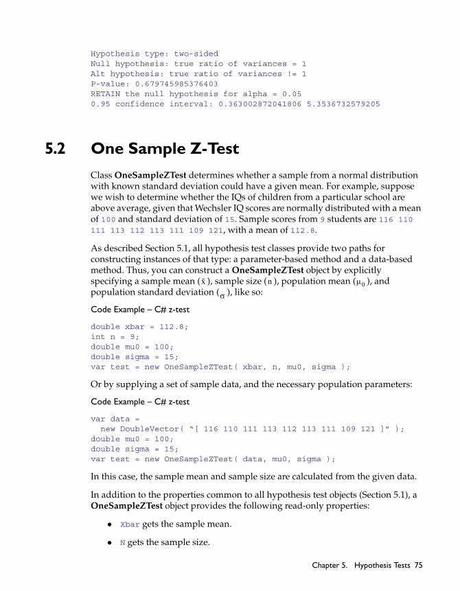
Hypothesis type: two-sidedNull hypothesis: true ratio of variances = 1Alt hypothesis: true ratio of variances != 1P-value: 0.679745985376403RETAIN the null hypothesis for alpha = 0.050.95 confidence interval: 0.363002872041806 5.3536732579205
5.2 One Sample Z-Test
Class OneSampleZTest determines whether a sample from a normal distribution with known standard deviation could have a given mean. For example, suppose we wish to determine whether the IQs of children from a particular school are above average, given that Wechsler IQ scores are normally distributed with a mean of 100 and standard deviation of 15. Sample scores from 9 students are 116 110 111 113 112 113 111 109 121, with a mean of 112.8.
As described Section 5.1, all hypothesis test classes provide two paths for constructing instances of that type: a parameter-based method and a data-based method. Thus, you can construct a OneSampleZTest object by explicitly specifying a sample mean ( ), sample size ( ), population mean ( ), and population standard deviation ( ), like so:
Code Example – C# z-test
double xbar = 112.8;int n = 9;double mu0 = 100;double sigma = 15;var test = new OneSampleZTest( xbar, n, mu0, sigma );
Or by supplying a set of sample data, and the necessary population parameters:
Code Example – C# z-test
var data = new DoubleVector( “[ 116 110 111 113 112 113 111 109 121 ]” );double mu0 = 100;double sigma = 15;var test = new OneSampleZTest( data, mu0, sigma );
In this case, the sample mean and sample size are calculated from the given data.
In addition to the properties common to all hypothesis test objects (Section 5.1), a OneSampleZTest object provides the following read-only properties:
Xbar gets the sample mean.
N gets the sample size.
x n 0
Chapter 5. Hypothesis Tests 75
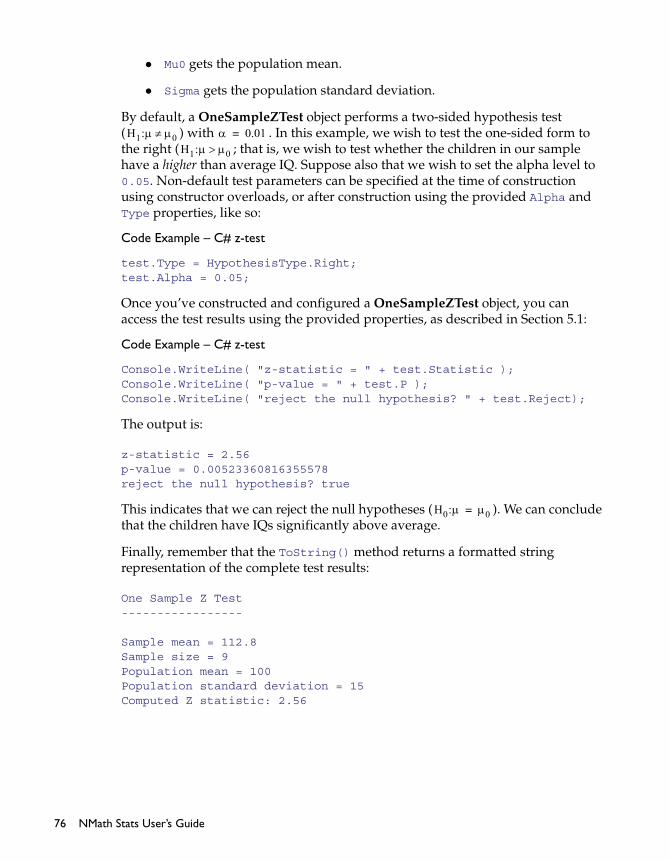
Mu0 gets the population mean.
Sigma gets the population standard deviation.
By default, a OneSampleZTest object performs a two-sided hypothesis test ( ) with . In this example, we wish to test the one-sided form to the right ( ; that is, we wish to test whether the children in our sample have a higher than average IQ. Suppose also that we wish to set the alpha level to 0.05. Non-default test parameters can be specified at the time of construction using constructor overloads, or after construction using the provided Alpha and Type properties, like so:
Code Example – C# z-test
test.Type = HypothesisType.Right;test.Alpha = 0.05;
Once you’ve constructed and configured a OneSampleZTest object, you can access the test results using the provided properties, as described in Section 5.1:
Code Example – C# z-test
Console.WriteLine( "z-statistic = " + test.Statistic );Console.WriteLine( "p-value = " + test.P );Console.WriteLine( "reject the null hypothesis? " + test.Reject);
The output is:
z-statistic = 2.56p-value = 0.00523360816355578reject the null hypothesis? true
This indicates that we can reject the null hypotheses ( ). We can conclude that the children have IQs significantly above average.
Finally, remember that the ToString() method returns a formatted string representation of the complete test results:
One Sample Z Test-----------------
Sample mean = 112.8Sample size = 9Population mean = 100Population standard deviation = 15Computed Z statistic: 2.56
H1: 0 0.01=H1: 0
H0: 0=
76 NMath Stats User’s Guide

Hypothesis type: one-sided to the rightNull hypothesis: sample mean = population meanAlt hypothesis: sample mean > population meanP-value: 0.00523360816355578REJECT the null hypothesis for alpha = 0.050.95 confidence interval: 104.575731865243 Infinity
5.3 One Sample T-Test
Class OneSampleTTest determines whether a sample from a normal distribution with unknown standard deviation could have a given mean. For example, suppose we wish to determine whether the self-esteem of children from a particular school differ from average, given a known population value of 3.9 on the Rosenberg Self-Esteem Scale. 113 children are tested, with a mean score of 4.0408 and a standard deviation of .6542.
As described Section 5.1, all hypothesis test classes provide two paths for constructing instances of that type: a parameter-based method and a data-based method. Thus, you can construct a OneSampleTTest object by explicitly specifying a sample mean ( ), sample standard deviation ( ), sample size ( ), and population mean ( ), like so:
Code Example – C# t-test
double xbar = 4.0408;double s = .6542;int n = 113;double mu0 = 3.9;var test = new OneSampleTTest( xbar, s, n, mu0 );
Or by supplying a set of sample data, and the necessary population parameters. For instance, if the sample data is in column 3 of DataFrame df:
Code Example – C# t-test
double mu0 = 3.9;var test = new OneSampleTTest( df[3], mu0 );
In this case, the sample mean, standard deviation, and size are calculated from the given data.
In addition to the properties common to all hypothesis test objects (Section 5.1), a OneSampleTTest object provides the following read-only properties:
Xbar gets the sample mean.
S gets the sample standard deviation.
N gets the sample size.
x s n0
Chapter 5. Hypothesis Tests 77

Mu0 gets the population mean.
DegreesOfFreedom gets the degrees of freedom.
By default, a OneSampleTTest object performs a two-sided hypothesis test ( ) with . Non-default test parameters can be specified at the time of construction using constructor overloads, or after construction using the provided Alpha and Type properties, like so:
Code Example – C# t-test
test.Alpha = 0.05;
Once you’ve constructed and configured a OneSampleTTest object, you can access the various test results using the provided properties, as described in Section 5.1:
Code Example – C# t-test
Console.WriteLine( "t-statistic = " + test.Statistic );Console.WriteLine( "deg of freedom = " + test.DegreesOfFreedom );Console.WriteLine( "p-value = " + test.P );Console.WriteLine( "reject the null hypothesis? " + test.Reject);
The output is:
t-statistic = 2.28786996397591deg of freedom = 112p-value = 0.0240223660991041reject the null hypothesis? True
This indicates that we can reject the null hypotheses ( ). We can conclude that the children have self-esteem scores significantly different than average.
Finally, remember that the ToString() method returns a formatted string representation of the complete test results:
One Sample t Test-----------------
Sample mean = 4.0408Sample standard deviation = 0.6542Sample size = 113Population mean = 3.9Computed t statistic: 2.28786996397591, df = 112
Hypothesis type: two-sidedNull hypothesis: sample mean = population meanAlt hypothesis: sample mean != population meanP-value: 0.0240223660991041REJECT the null hypothesis for alpha = 0.050.95 confidence interval: 3.91886249658971 4.16273750341029
H1: 0 0.01=
H0: 0=
78 NMath Stats User’s Guide

5.4 Two Sample Paired T-Test
Class TwoSamplePairedTTest tests the null hypothesis that the population mean of the paired differences of two samples is zero. Pairing involves matching up individuals in two samples so as to minimize their dissimilarity except in the factor under study. Paired samples often occur in pre-test/post-test studies in which subjects are measured before and after an intervention. They also occur in matched-pairs (for example, matching on age and sex), cross-over trials, and sequential observational samples. Paired samples are also called matched samples and dependent samples.
NOTE—TwoSamplePairedTTest is equivalent to performing a OneSampleTTest on the paired differences (see Section 5.3).
For example, suppose we measure the thickness of plaque (mm) in the carotid artery of 10 randomly selected patients with mild atherosclerotic disease. Two measurements are taken: before treatment with Vitamin E (baseline), and after two years of taking Vitamin E daily. The mean difference between paired measurements is 0.045 with a standard deviation of 0.0264.
As described Section 5.1, all hypothesis test classes provide two paths for constructing instances of that type: a parameter-based method and a data-based method. Thus, you can construct a TwoSamplePairedTTest object by explicitly specifying the mean difference between paired observations ( ), the standard deviation of the differences ( ), and the sample size ( ), like so:
Code Example – C# paired t-test
double xbar = 0.045;double s = 0.0264;int n = 10;var test = new TwoSamplePairedTTest( xbar, s, n );
Alternatively, you can supply two sets of sample data. For instance, this code adds data to a DataFrame (Chapter 2):
Code Example – C# paired t-test
var df = new DataFrame();df.AddColumn( new DFNumericColumn( "Baseline" ) );df.AddColumn( new DFNumericColumn( "Vit E" ) );
xs n
Chapter 5. Hypothesis Tests 79

df.AddRow( 1, 0.66, 0.60 );df.AddRow( 2, 0.72, 0.65 );df.AddRow( 3, 0.85, 0.79 );df.AddRow( 4, 0.62, 0.63 );df.AddRow( 5, 0.59, 0.54 );df.AddRow( 6, 0.63, 0.55 );df.AddRow( 7, 0.64, 0.62 );df.AddRow( 8, 0.70, 0.67 );df.AddRow( 9, 0.73, 0.68 );df.AddRow( 10, 0.68, 0.64 );
And this code constructs a TwoSamplePairedTTest from the two columns of data:
Code Example – C# paired t-test
TwoSamplePairedTTest test = new TwoSamplePairedTTest( df[ “Baseline” ], df[ “Vit E” ] );
The mean difference between paired measurements, the standard deviation, and the sample size are calculated from the given data.
In addition to the properties common to all hypothesis test objects (Section 5.1), a TwoSamplePairedTTest object provides the following read-only properties:
Xbar gets the mean of the differences between paired observations.
S gets the standard deviation of the differences between paired observations.
N gets the number of pairs.
DegreesOfFreedom gets the degrees of freedom.
By default, a TwoSamplePairedTTest object performs a two-sided hypothesis test ( ) with . Non-default test parameters can be specified at the time of construction using constructor overloads, or after construction using the provided Type and Alpha properties.
Once you’ve constructed and configured a TwoSamplePairedTTest object, you can access the various test results using the provided properties, as described in Section 5.1:
Code Example – C# paired t-test
Console.WriteLine( "t-statistic = " + test.Statistic );Console.WriteLine( "deg of freedom = " + test.DegreesOfFreedom );Console.WriteLine( "p-value = " + test.P );Console.WriteLine( "reject the null hypothesis? " + test.Reject);
H1:d 0 0.01=
80 NMath Stats User’s Guide

The output is:
t-statistic = 5.4deg of freedom = 9p-value = 0.000433006432003502reject the null hypothesis? True
This indicates that we can reject the null hypotheses ( ). We can conclude that the true mean thickness of plaque after two years treatment with Vitamin E is significantly different than before treatment.
Finally, remember that the ToString() method returns a formatted string representation of the complete test results:
Two Sample t Test (Paired)--------------------------
Mean of differences between pairs = 0.045Standard deviation of differences between pairs = 0.0263523138347365Sample size (number of pairs) = 10Computed t statistic: 5.4, df = 9
Hypothesis type: two-sidedNull hypothesis: true mean of differences between pairs = 0Alt hypothesis: true mean of differences between pairs != 0P-value: 0.000433006432003502REJECT the null hypothesis for alpha = 0.010.99 confidence interval: 0.0179180371533991 0.0720819628466008
5.5 Two Sample Unpaired T-Test
Class TwoSampleUnpairedTTest tests whether two samples from a normal distribution could have the same mean when the standard deviations are unknown but assumed to be equal, allowing for a pooled estimate of the variance.
Class TwoSampleUnpairedUnequalTTest assumes that the samples may come from populations with unequal variances, and the Welch-Satterthwaite approximation to the degrees of freedom is used. Unlike TwoSampleUnpairedTTest, a pooled estimate of the variance is not used.
For example, suppose we work for a company that makes plastic widgets and we want to compare plastic samples from two suppliers for strength. We record the breaking strength in psi (pounds per square inch) for random samples from each supplier and obtain the following data: 11 samples from the first supplier having a mean strength of 4.2 psi and a standard deviation of 4.68; 8 samples from the second supplier have a mean strength of 5.6 and a standard deviation of 3.92.
H0:d 0=
Chapter 5. Hypothesis Tests 81

As described Section 5.1, all hypothesis test classes provide two paths for constructing instances of that type: a parameter-based method and a data-based method. Thus, you can construct a TwoSampleUnpairedTTest object by explicitly specifying the mean ( ), standard deviation ( ), and size ( ) of each sample, like so:
Code Example – C# unpaired t-test
double xbar1 = 4.2;double s1 = 4.68;int n1 = 11;
double xbar2 = 5.6;double s2 = 3.92;int n2 = 8;
var test = new TwoSampleUnpairedTTest( xbar1, s1, n1, xbar2, s2, n2 );
Or by supplying two sets of sample data. For instance, if the sample data is in two vectors supplier1 and supplier2:
Code Example – C# unpaired t-test
var test = new TwoSampleUnpairedTTest( supplier1, supplier2 );
The sample means, standard deviations, and sizes are calculated from the given data.
In addition to the properties common to all hypothesis test objects (Section 5.1), a TwoSampleUnpairedTTest object provides the following read-only properties:
Xbar1 and Xbar2 get the means of the samples.
S1 and S2 get the standard deviations of the samples.
SPooled gets the pooled estimate of the standard deviation.
N1 and N2 get the sizes of the samples.
DegreesOfFreedom gets the degrees of freedom.
By default, a TwoSampleUnpairedTTest object performs a two-sided hypothesis test ( ) with . Non-default test parameters can be specified at the time of construction using constructor overloads, or after construction using the provided Type and Alpha properties.
Once you’ve constructed and configured a TwoSampleUnpairedTTest object, you can access the various test results using the provided properties, as described in Section 5.1:
x s n
H1:1 2– 0 0.01=
82 NMath Stats User’s Guide
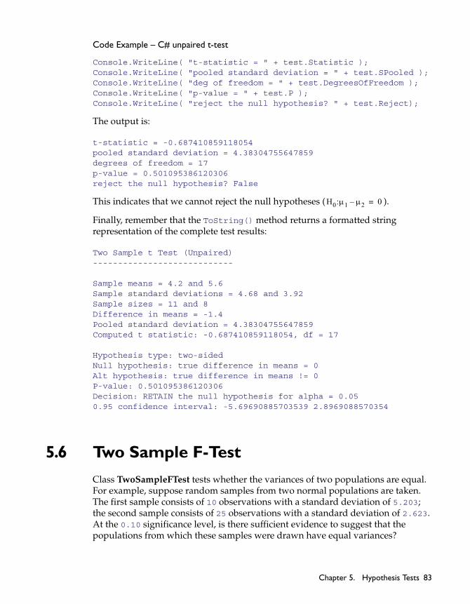
Code Example – C# unpaired t-test
Console.WriteLine( "t-statistic = " + test.Statistic );Console.WriteLine( "pooled standard deviation = " + test.SPooled );Console.WriteLine( "deg of freedom = " + test.DegreesOfFreedom );Console.WriteLine( "p-value = " + test.P );Console.WriteLine( "reject the null hypothesis? " + test.Reject);
The output is:
t-statistic = -0.687410859118054pooled standard deviation = 4.38304755647859degrees of freedom = 17p-value = 0.501095386120306reject the null hypothesis? False
This indicates that we cannot reject the null hypotheses ( ).
Finally, remember that the ToString() method returns a formatted string representation of the complete test results:
Two Sample t Test (Unpaired)----------------------------
Sample means = 4.2 and 5.6Sample standard deviations = 4.68 and 3.92Sample sizes = 11 and 8Difference in means = -1.4Pooled standard deviation = 4.38304755647859Computed t statistic: -0.687410859118054, df = 17
Hypothesis type: two-sidedNull hypothesis: true difference in means = 0Alt hypothesis: true difference in means != 0P-value: 0.501095386120306Decision: RETAIN the null hypothesis for alpha = 0.050.95 confidence interval: -5.69690885703539 2.8969088570354
5.6 Two Sample F-Test
Class TwoSampleFTest tests whether the variances of two populations are equal. For example, suppose random samples from two normal populations are taken. The first sample consists of 10 observations with a standard deviation of 5.203; the second sample consists of 25 observations with a standard deviation of 2.623. At the 0.10 significance level, is there sufficient evidence to suggest that the populations from which these samples were drawn have equal variances?
H0:1 2– 0=
Chapter 5. Hypothesis Tests 83

As described Section 5.1, all hypothesis test classes provide two paths for constructing instances of that type: a parameter-based method and a data-based method. Thus, you can construct a TwoSampleFTest object by explicitly specifying the standard deviation ( ),and size ( ) of each sample, like so:
Code Example – C# F-test
double s1 = 5.203;int n1 = 10;
double s2 = 2.623;int n2 = 25;
var test = new TwoSampleFTest( s1, n1, s2, n2 );
Or by supplying two sets of sample data. For instance, if the sample data is in two vectors v1 and v2:
Code Example – C# F-test
var test = new TwoSampleFTest( v1, v2 );
The sample standard deviations and sizes are calculated from the given data.
In addition to the properties common to all hypothesis test objects (Section 5.1), a TwoSampleFTest object provides the following read-only properties:
S1 and S2 get the standard deviations of the samples.
N1 and N2 get the sizes of the samples.
DegreesOfFreedom1 gets the numerator degrees of freedom.
DegreesOfFreedom2 gets the denomenator degrees of freedom.
By default, a TwoSampleFTest object performs a two-sided hypothesis test ( ) with . Non-default test parameters can be specified at the time of construction using constructor overloads, or after construction using the provided Type and Alpha properties.
Once you’ve constructed and configured a TwoSampleFTest object, you can access the various test results using the provided properties, as described in Section 5.1:
Code Example – C# F-test
Console.WriteLine( "t-statistic = " + test.Statistic );Console.WriteLine( "numerator df = " + test.DegreesOfFreedom1 );Console.WriteLine( "denomenator df = " + test.DegreesOfFreedom2 );Console.WriteLine( "p-value = " + test.P );Console.WriteLine( "reject the null hypothesis? " + test.Reject);
s n
H1:s12
s22 1 0.01=
84 NMath Stats User’s Guide

The output is:
F-statistic = 3.93469497446923numerator df = 9denomenator df = 24p-value = 0.00693561186501657reject the null hypothesis? True
This indicates that we cannot reject the null hypotheses ( ).
Finally, remember that the ToString() method returns a formatted string representation of the complete test results:
Two Sample F Test-----------------
Sample Sizes = 10 and 25Standard Deviations = 5.203 and 2.623Variances = 27.071209 and 6.880129Computed F statistic: 3.93469497446923, num df = 9, denom df = 24
Hypothesis type: two-sidedNull hypothesis: true ratio of variances = 1Alt hypothesis: true ratio of variances != 1P-value: 0.00693561186501657REJECT the null hypothesis for alpha = 0.010.99 confidence interval: 1.06490202325594 22.5425454339445
5.7 Pearson’s Chi-Square Test
NMath Stats provides class PearsonsChiSquareTest for performing Pearson's chi-square test. Pearson's chi-square test is the most well-known of the chi-square tests, which are statistical procedures whose results are evaluated by reference to the chi-square distribution. It tests the null hypothesis that the frequency distribution of experimental outcomes are consistent with a particular theoretical distribution. The event outcomes considered must be mutually exclusive and have a total probability of 1.
Instances of PearsonsChiSquareTest are constructed either from raw data or tables of counts. For example, this code constructs a PearsonsChiSquareTest using outcomes from a series of experiment runs, along with the expected frequencies:
Code Example – C# chi-square test
int[] outcomes = { 59, 20, 11, 10 };DoubleVector probs = new DoubleVector( 0.5625, 0.1875, 0.1875, 0.0625 );
H0:s12
s22 1=
Chapter 5. Hypothesis Tests 85

PearsonsChiSquareTest test = new PearsonsChiSquareTest( outcomes, probs );
This code uses a contingency table (or cross tabulation) to store the relation between two or more categorical variables:
Code Example – C# chi-square test
var data = new int[2, 2];data[0, 0] = 4298;data[0, 1] = 767;data[1, 0] = 7136;data[1, 1] = 643;bool yatesCorrect = true;PearsonsChiSquareTest test = new PearsonsChiSquareTest( data, yatesCorrect );
The Yates’ correction for continuity may optionally be applied.
Once you’ve constructed and configured a PearsonsChiSquareTest object, you can access the various test results using the provided properties, as described in Section 5.1:
Code Example – C# chi-square test
Console.WriteLine( "chi-square statistic = " + test.ChiSquareStatistic );Console.WriteLine( "numerator df = " + test.DegreesOfFreedom );Console.WriteLine( "p-value = " + test.P );Console.WriteLine( "reject the null hypothesis? " + test.Reject );
The output is:
chi-square statistic = 147.761248704421numerator df = 1p-value = 0reject the null hypothesis? True
Again, the ToString() method returns a formatted string representation of the complete test results:
Pearson chi-square test-----------------
Sample size = 12844Yates corrected = TrueComputed chi-square statistic: 147.761248704421, df = 1
P-value: 0REJECT the null hypothesis for alpha = 0.01
86 NMath Stats User’s Guide
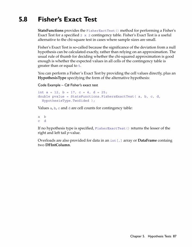
5.8 Fisher’s Exact Test
StatsFunctions provides the FisherEactTest() method for performing a Fisher's Exact Test for a specified 2 x 2 contingency table. Fisher's Exact Test is a useful alternative to the chi-square test in cases where sample sizes are small.
Fisher's Exact Test is so-called because the significance of the deviation from a null hypothesis can be calculated exactly, rather than relying on an approximation. The usual rule of thumb for deciding whether the chi-squared approximation is good enough is whether the expected values in all cells of the contingency table is greater than or equal to 5.
You can perform a Fisher’s Exact Test by providing the cell values directly, plus an HypothesisType specifying the form of the alternative hypothesis:
Code Example – C# Fisher’s exact test
int a = 12, b = 17, c = 4, d = 25;double pvalue = StatsFunctions.FishersExactTest( a, b, c, d, HypothesisType.TwoSided );
Values a, b, c and d are cell counts for contingency table:
a bc d
If no hypothesis type is specified, FisherExactTest() returns the lesser of the right and left tail p-value.
Overloads are also provided for data in an int[,] array or DataFrame containg two DFIntColumn.
Chapter 5. Hypothesis Tests 87

88 NMath Stats User’s Guide

CHAPTER 6. LINEAR REGRESSION
Class LinearRegression computes a multiple linear regression from an input matrix of independent variable values (the predictor matrix or regression matrix) and a vector of dependent variable values (the observation vector).
In a linear model, a quantity y depends on one or more independent variables a1, a2,...,an such that y = x0 + x1a1 + ... + xnan. (Parameter x0 is called the intercept parameter.) Several observations of the independent values ai are recorded, along with the corresponding values of the dependent variable y. If m observations are performed, and for the ith observation we denote the values of the independent variables ai1, ai2,...,ain and the corresponding dependent value of y as yi, then we form the linear system Ax = y, where matrix A = (aij) and vector y = (yi). The regression solution is the value of x that minimizes ||Ax - y||.
This chapter describes how to use the LinearRegression class, and related supporting classes.
6.1 Creating Linear Regressions
A LinearRegression instance is constructed from a predictor matrix and observation vector, like so:
Code Example – C# linear regression
DoubleMatrix predictors = new DoubleMatrix( “ 8x4 [ 1 1450 .50 70 1 1600 .50 70 1 1450 .70 70 1 1600 .70 70 1 1450 .50 120 1 1600 .50 120 1 1450 .70 120 1 1600 .70 120 ]” );
Chapter 6. Linear Regression 89

DoubleVector obs = new DoubleVector( “[ 67 79 61 75 59 90 52 87 ]” );var lr = new LinearRegression( predictors, obs );
A MismatchedSizeException is raised if the number of rows in the matrix A is not equal to the length of the vector obs.
You can also construct a LinearRegression instance from data in a DataFrame, by indicating which column contains the observations. Non-numeric columns are ignored. For instance, if column 8 contains the dependent variable, this code constructs a regression from the data:
Code Example – C# linear regression
var lr = new LinearRegression( df, 8 );
Parameter Calculation by Least Squares Minimization
By default, class LinearRegression computes the model parameter values by the method of least squares using a QR factorization, but you may elect to use a complete orthogonal factorization or singular value decomposition instead.
IRegressionCalculation is the interface for classes used by LinearRegression to calculate regression parameters. NMath Stats includes three regression calculator classes:
Class QRRegressionCalculation (the default) solves the regression problem using a QR decomposition.
Class SVDRegressionCalculation solves the regression problem using a singular value decomposition.
Class CORegressionCalculation solves least squares problems using a complete orthogonal decomposition.
You can specify a non-default regression calculation object in the constructor. For example:
Code Example – C# linear regression
var calcObj = new CORegressionCalculation();calcObj.Tolerance = 1e-8;var lr = new LinearRegression( predictors, obs, calcObj );
The Tolerance property is used for computing numerical rank. Values with less than the specified tolerance are considered zero when computing the effective rank.
After construction, the regression calculator used by a LinearRegression instance can be changed using the RegressionCalculator property.
90 NMath Stats User’s Guide
Intercept Parameters
If the linear model Ax = y contains a non-zero intercept parameter, then the first column of matrix A must be all ones. Some of the LinearRegression constructors allow you to specify whether a column of ones should be prepended to the data in the input regression matrix, or whether the regression matrix should be used as it is given. Thus, this code prepends a column of ones:
Code Example – C# linear regression
LinearRegression lr = new LinearRegression( predictors, obs, true );
This code does not:
Code Example – C# linear regression
LinearRegression lr = new LinearRegression( predictors, obs, false );
6.2 Regression Results
Class LinearRegression provides the following properties for accessing the regression results:
IsGood gets a boolean value indicating whether or not the model parameters were successfully computed.
ParameterCalculationErrorMessage gets any error message produced by the regression calculation object.
Parameters gets the vector of computed model parameters.
ParameterEstimates gets an array of LinearRegressionParameter objects suitable for performing hypothesis testing on individual parameters (see Section 6.5).
Residuals gets the vector of residuals. This is the difference between the vector of observed values and the values predicted by the model.
Variance gets an estimate of the variance. This is the residual sum of squares divided by the degrees of freedom for the model. The degrees of freedom for the model is equal to the difference between the number of observations and the number of parameters.
CovarianceMatrix gets the covariance matrix (sometimes called the dispersion matrix or variance-covariance matrix).
Chapter 6. Linear Regression 91

GetStandardizedResiduals() gets the standardized residuals (also known as the internally studentized residuals). The residuals are renormalized to have unit variance using an overall measure of error variance.
GetStudentizedResiduals() gets the (externally) studentized residuals, which renormalizes the residuals to have unit variance using a leave-one-out measure of error variance—that is, a vector of estimates of the residual variance obtained when the i-th case is dropped from the regression.
For more information about a linear regression fit, you can perform hypothesis tests on individual parameters (Section 6.5) or the overall model (Section 6.6).
You can also modify the model and recalculate the parameters, as described in Section 6.4.
Variance Inflation Factor
The variance inflation factor (VIF) quantifies the severity of multicollinearity in a least squares regression analysis—that is, how much the variance of a coefficient is increased because of collinearity. Class LinearRegression provides methods VarianceInflationFactor() and VarianceInflationFactors() for this purpose. For instance:
Code Example – C# linear regression
DoubleVector vif = lr.VarianceInflationFactors();
6.3 Predictions
You can use a LinearRegression object to generate predictions. The PredictedObservation() method returns the response predicted by the model for a given set of predictor variable values. For example:
Code Example – C# linear regression
DoubleVector predictors = new DoubleVector( 150.0, 33.5, 0.66, 80.0 );double predicted = lr.PredictedObservation( predictors );
A MismatchedSizeException is raised if the length of the given vector is not equal to the number of parameters in the model.
Similarly, the PredictedObservations() method returns the responses predicted by the model for a given collection of predictors:
92 NMath Stats User’s Guide

Code Example – C# linear regression
DoubleMatrix predictors = new DoubleMatrix( "3x4 [ 150.0 33.5 0.66 80.0 160.0 24.5 0.88 70.0 170.0 22.6 0.56 60.0 ]" );DoubleVector predicted = lr.PredictedObservations( predictors );
In the returned vector of predicted observations, the ith element is the predicted response for the set of predictor variable values in the ith row of the given matrix.
6.4 Accessing and Modifying the Model
Class LinearRegression provides a variety of properties and member functions for accessing and modifying the predictors in the model, the observations, and the intercept option.
Accessing and Modifying Predictors
Class LinearRegression provides the following properties for accessing the predictors in the model:
RegressionMatrix gets the regression matrix.
PredictorMatrix gets the predictor matrix. If the model contains an intercept parameter, then the predictor matrix is obtained from the regression matrix by removing the leading column of ones. If the model does not have an intercept parameter then the predictor matrix is the same as the regression matrix.
NumberOfParameters gets the number of parameters in the model.
NumberOfPredictors gets the number of predictors in the model. If the model contains an intercept parameter then the number of predictors is equal to the number of parameters minus one. If the model does not contain an intercept parameter, then the number of predictors is equal to the number of parameters.
If you modify the data in the regression or predictor matrix using the reference returned by RegressionMatrix or PredictorMatrix, respectively, invoke method RecalculateParameters() to recalculate the regression parameters. For instance:
Code Example – C# linear regression
lr.PredictorMatrix[2,13] = 15.4;lr.RecalculateParameters();
Chapter 6. Linear Regression 93
Member functions are also provided for adding and removing one or more predictors. The AddPredictor() method appends a given column of predictor values to the predictor matrix, and recalculates the parameters:
Code Example – C# linear regression
DoubleVector predictors = new DoubleVector( “[ 1.43 5.5 0.43 14.2 9.0 ]” );
lr.AddPredictor( predictors );
A MismatchedSizeException is thrown if the number of predictor values is not equal to the number of rows in the regression matrix (also equal to the length of the observation vector).
Similarly, AddPredictors() adds a matrix of predictors. Each column of the input matrix is a set of observed predictor values. This, this code adds three predictors:
Code Example – C# linear regression
DoubleMatrix predictors = new DoubleMatrix( “ 8x3 [ 1450 .50 70 1600 .50 70 1450 .70 70 1600 .70 70 1450 .50 120 1600 .50 120 1450 .70 120 1600 .70 120 ]” );lr.AddPredictor( predictors );
The RemovePredictor() method removes the ith predictor from the model and recalculates the parameters. This code removes the predictor at (zero-based) index 4:
Code Example – C# linear regression
lr.RemovePredictor( 4 );
If the model has an intercept parameter, removing the 0th predictor will not remove the intercept parameter. Use the RemoveInterceptParameter() method to remove the intercept parameter (see below).
RemovePredictors() removes the specified number of columns from the predictor matrix beginning with the specified column. Thus, this code removes the second, third, and fourth predictors:
Code Example – C# linear regression
lr.RemovePredictors( 1, 3 );
94 NMath Stats User’s Guide

Accessing and Modifying Observations
The Observations property gets the vector of observations. If you use the returned reference to modify the observation vector, invoke method RecalculateParameters() to recalculate the regression parameters. For instance:
Code Example – C# linear regression
lr.Observations[5] = 0.965;lr.RecalculateParameters();
The NumberOfObservations property gets the number of observations, which is simply the length of the observation vector, and also the number of rows in the regression matrix.
Member functions are also provided for adding and removing one or more observations. The AddObservation() method appends a given row of predictor values to the predictor matrix and a given observation to the observation vector, and recalculates the parameters:
Code Example – C# linear regression
DoubleVector predictors = new DoubleVector( “[ 1.43 5.5 0.43 14.2 9.0 ]” );double obs = 2.5;
lr.AddObservation( predictors, obs );
NOTE—If the model has an intercept parameter, do not include the leading one in the predictors vector. It will be accounted for in the model.
A MismatchedSizeException is thrown if the length of the predictors vector is not equal to the number of predictors in the model.
Similarly, AddObservations() adds a collection of observations:
Code Example – C# linear regression
var predictors = new DoubleMatrix( "3x4 [ 150.0 33.5 0.66 80.0 160.0 24.5 0.88 70.0 170.0 22.6 0.56 60.0 ]" );var obs = new DoubleVector( “14.2, 15.5, 10.3” );
lr.AddObservation( predictors, obs );
RemoveObservation() removes the row at the indicated index from the predictor matrix and the corresponding element from the observation vector. This code removes the observation at (zero-based) index 3:
Chapter 6. Linear Regression 95

Code Example – C# linear regression
lr.RemoveObservation( 3 );
RemoveObservations() removes the specified number of rows from the predictor matrix beginning with the specified row. Thus, this code removes the third, fourth, fifth, and sixth observations:
Code Example – C# linear regression
lr.RemoveObservations( 2, 4 );
Accessing and Modifying the Intercept Option
The HasInterceptParameter property gets a boolean value indicating whether or not the model already has an intercept parameter.
The AddInterceptParameter() method adds an intercept parameter to the model and recalculates the parameters. Thus, this code prepends a column of one to the regression matrix:
Code Example – C# linear regression
lr.AddInterceptParameter()
NOTE—If the model already has an intercept parameter AddInterceptParameter() has no effect.
The RemoveInterceptParameter() method removes the intercept parameter.
Updating the Entire Model
Method SetRegressionData() updates the entire model by setting the regression matrix, the observation vector, and the intercept option to the specified values, and recalculating the model parameters. For instance:
Code Example – C# linear regression
var A = new DoubleMatrix( “ 8x4 [ 1 1450 .50 70 1 1600 .50 70 1 1450 .70 70 1 1600 .70 70 1 1450 .50 120 1 1600 .50 120 1 1450 .70 120 1 1600 .70 120 ]” );var obs = new DoubleVector( “[ 67 79 61 75 59 90 52 87 ]” );
lr.SetRegressionData( A, obs, true );
96 NMath Stats User’s Guide

6.5 Significance of Parameters
Instances of class LinearRegressionParameter test statistical hypothesis about individual parameters in a LinearRegression.
Creating Linear Regression Parameter Objects
You can construct a LinearRegressionParameter from a LinearRegression object and the index of the parameter you wish to test. For instance, this code creates a test object for the third parameter:
Code Example – C# linear regression
LinearRegressionParameter param = new LinearRegressionParameter( lr, 2 );
Alternatively, you can get an array of test objects for all parameters in a linear regression using the ParameterEstimates property on LinearRegression:
Code Example – C# linear regression
LinearRegressionParameter[] params = lr.ParameterEstimates;
Properties Linear Regression Parameters
Class LinearRegressionParameter provides the following properties:
Value gets the value of the parameter.
StandardError gets the standard error of the parameter.
ParameterIndex gets the index of the parameter in the linear regresssion.
Hypothesis Tests
Class LinearRegressionParameter provides the following methods for testing statistical hypotheses regarding parameter values:
TStatisticPValue() returns the p-value for a two-sided t test with the null hypothesis that the parameter is equal to a given test value, versus the alternative hypothesis that it is not.
TStatistic() returns the value of the t statistic for the null hypothesis that the parameter value is equal to a given test value.
TStatisticCriticalValue() gets the critical value for the t-statistic for a given alpha level.
Chapter 6. Linear Regression 97

ConfidenceInterval() returns a confidence interval for the parameter for a given alpha level.
For example, this code tests whether the fifth parameter in a model is significantly different than zero:
Code Example – C# linear regression
LinearRegressionParameter param = new LinearRegressionParameter( lr, 4 );double tstat = param.TStatistic( 0.0 );double pValue = param.TStatisticPValue( 0.0 );double criticalValue = param.TStatisticCriticalValue( 0.05 );Interval confidenceInterval = param.ConfidenceInterval( 0.05 );
Updating Linear Regression Parameters
The SetRegression() method updates the regression and parameter index in a parameter test object:
Code Example – C# linear regression
param.SetRegression( lr, 6 );
6.6 Significance of the Overall Model
Class LinearRegressionAnova tests the overall model significance for linear regressions. Simply construct a LinearRegressionAnova from a LinearRegression object:
Code Example – C# linear regression
var lrAnova = new LinearRegressionAnova( lr );
A variety of properties are provided for assessing the significance of the overall model:
RegressionSumOfSquares gets the regression sum of squares. This quantity indicates the amount of variability explained by the model. It is the sum of the squares of the difference between the values predicted by the model and the mean.
ResidualSumOfSquares gets the residual sum of squares. This is the sum of the squares of the differences between the predicted and actual observations.
ModelDegreesOfFreedom gets the number of degrees of freedom for the model, which is equal to the number of predictors in the model.
1 –
98 NMath Stats User’s Guide

ErrorDegreesOfFreedom gets the number of degress of freedom for the model error, which is equal to the number of observations minus the number of model paramters.
RSquared gets the coefficient of determination.
AdjustedRsquared gets the adjusted coefficient of determination.
MeanSquaredResidual gets the mean squared residual. This quantity is the equal to ResidualSumOfSquares / ErrorDegreesOfFreedom (equals the number of observations minus the number of model parameters).
MeanSquaredRegression gets the mean squared for the regression. This is equal to RegressionSumOfSquares / ModelDegreesOfFreedom (equals the number of predictors in the model).
FStatistic gets the overall F statistic for the model. This is equal to the ratio of MeanSquaredRegression / MeanSquaredResidual. This is the statistic for the hypothesis test where the null hypothesis, is that all the parameters are equal to 0 and the alternative hypothesis is that at least one paramter is nonzero.
FStatisticPValue gets the p-value for the F statistic.
For example:
Code Example – C# linear regression
var lrAnova = new LinearRegressionAnova( lr );double sse = lrAnova.ResidualSumOfSquares;double r2 = lrAnova.RSquared;double fstat = lrAnova.FStatistic;double fstatPval = lrAnova.FStatisticPValue;
Lastly, the FStatisticCriticalValue() function computes the critical value for the F statistic at a given significance level:
Code Example – C# linear regression
double critVal = lrAnova.FStatisticCriticalValue(.05);
H0
Chapter 6. Linear Regression 99

100 NMath Stats User’s Guide
CHAPTER 7. LOGISTIC REGRESSION
Class LogisticRegression performs a binomial logistic regression.
Logistic regression is used to model the relationship between a binary response variable and one or more predictor variables, which may be either discrete or continuous. Binary outcome data is common in medical applications. For example, the binary response variable might indicate whether or not a patient is alive five years after treatment for cancer or whether the patient has an adverse reaction to a new drug. As in multiple linear regression (Chapter 6), we are interested in finding an appropriate combination of predictor variables to help explain the binary outcome.
This chapter describes how to use the LogisticRegression class, and related supporting classes.
7.1 Regression Calculators
Class LogisticRegression is templatized on the ILogisticRegressionCalc calculator to use to calculate the parameters of the logistic regression model. Two implementations are provided:
NewtonRaphsonParameterCalc computes the parameters to maximize the log likelihood function for the model using the Newton Raphson algorithm to compute the zeros of the first order partial derivatives of the log likelihood function. This algorithm is equivalent to, and sometimes referred to, as iteratively reweighted least squares. Each iteration involves solving a linear system of the form X'WX = b, where X is the regression matrix, X' is its transpose, and W is a diagonal matrix of weights.
The matrix X'WX will be singular if the matrix X does not have full rank. NewtonRaphsonParameterCalc has property FailIfNotFullRank which, if true, fails in this case. If FailIfNotFullRank is false, the linear system is solved using a pseudo-inverse, and the calculation will not fail.
Chapter 7. Logistic Regression 101

TrustRegionParameterCalc computes the parameters to maximize the log likelihood function for the model, using a trust region optimization algorithm to compute the zeros of the first order partial derivative of the log likelihood function. This approach is more robust than Newton Raphson with design matrices of less than full rank.
The minimization is performed by an instance of TrustRegionMinimizer, and TrustRegionParameterCalc instances may be constructed with a given minimizer with the desired algorithm properties.
7.2 Creating Logistic Regressions
A LogisticRegression object is constructed from data in the following format: a matrix whose rows contain the predictor variable values, and an IList<bool> for the observed values.
Code Example – C# logistic regression
DoubleMatrix A = ...bool[] obs = ...var lr = new LogisticRegression<NewtonRaphsonParameterCalc>( A, obs );
A MismatchedSizeException is raised if the number of rows in the matrix A is not equal to the length of the vector obs.
If you want the model to have an intercept parameter, you can specify that as well:
Code Example – C# logistic regression
bool addIntercept = true;var lr = new LogisticRegression<NewtonRaphsonParameterCalc>( A, obs, addIntercept );
If true, a column of ones is prepended onto the data in the regression matrix A, thus adding an intercept to the model. If false, the data in the regression matrix is used as given.
You can also provide a regression calculator instance to use. For example, if you want regression to fail consistently when the regression matrix is rank deficient, you can construct a NewtonRaphsonParameterCalc object with the FailIfNotFullRank property set to true (see Section 7.1), then construct a LogisticRegression object with the resulting parameter calculation object:
Code Example – C# logistic regression
var parameterCalc = new NewtonRaphsonParameterCalc() { FailIfNotFullRank = true };
102 NMath Stats User’s Guide

var lr = new LogisticRegression<NewtonRaphsonParameterCalc>( A, obs, addIntercept, parameterCalc );
Additional LogisticRegression constructors provide flexibility in how the observation values are specified. For example, you can provide a vector of floating point observation values, which is converted to dichotomous values using a supplied Predictate<double> function. This code uses a lambda expression to specify the predicate:
Code Example – C# logistic regression
DoubleVector v = ...var lr = new LogisticRegression<NewtonRaphsonParameterCalc>( A, v, x => x >= 110.0, addIntercept);
Similarly, you can provide the observation values as one of the columns of the regression matrix:
Code Example – C# logistic regression
int observationColIndex = 0;var lr = new LogisticRegression<NewtonRaphsonParameterCalc>( A, observationColIndex, x => x != 0, addIntercept);
Design Variables
LogisticRegression provides static convenience method DesignVariables() for producing design, or dummy, variables using reference cell coding. If the categorical variable has k levels, there will be k - 1 design variables created. Reference cell coding involves setting all the design variable values to 0 for the reference group, and then setting a single design variable equal to 1 for each of the other groups.
For example, suppose we have a DataFrame df with a column of race values, which has three levels.
Code Example – C# logistic regression
int raceColIndex = df.IndexOfColumn( "Race" );DataFrame raceDesignVars = LogisticRegression<NewtonRaphsonParameterCalc>.DesignVariables( df[raceColIndex] );
Since the race variable has three levels there will be two design variables. By default they will be named Race_0 and Race_1.
We then replace the original race column with the two design variable columns, and convert the data frame to a matrix of floating point values.
Code Example – C# logistic regression
df.RemoveColumn( raceColIndex );
Chapter 7. Logistic Regression 103
for ( int c = 0; c < raceDesignVars.Cols; c++ ){ df.InsertColumn( raceColIndex + c, raceDesignVars[c] );}DoubleMatrix matrixDat = data.ToDoubleMatrix();
7.3 Checking for Convergence
After constructing a LogisticRegression object, first check that the parameter calculation was successful. For example, this code checks the IsGood property, and if the calculation failed, prints out some diagnostic information using the ParameterCalculationErrorMessage property.
Code Example – C# logistic regression
if ( !lr.IsGood ){ Console.WriteLine( "Logistic regression parameter calculation failed:" ); Console.WriteLine( lr.ParameterCalculationErrorMessage );
var parameterCalc = lr.ParameterCalculator; Console.WriteLine( "Maximum iterations: " + parameterCalc.MaxIterations ); Console.WriteLine( "Number of iterations: " + parameterCalc.Iterations ); Console.WriteLine( "Converged? " + parameterCalc.Converged );}
7.4 Goodness of Fit
Class LogisticRegressionFitAnalysis calculates goodness of fit statistics for a logistic regression model.
Code Example – C# logistic regression
var fit = new LogisticRegressionFitAnalysis<NewtonRaphsonParameterCalc>( lr );
Provided properties access the model statistics:
GStatistic gets the G statistic for the model. The G statistic is
104 NMath Stats User’s Guide

G = -2*ln[(likelihood without the variables)/ (likelihood with the variables)]
GStatisticPValue gets the p-value for the G statistic.
LogLikelihood gets the log likelihood for the model.
For instance:
Code Example – C# logistic regression
Console.WriteLine( "Log likelihood: " + fit.LogLikelihood );Console.WriteLine( "G-statistic: " + fit.GStatistic );Console.WriteLine( "G-statistic P-value: " + fit.GStatisticPValue );
Two methods on LogisticRegressionFitAnalysis provide access to additional statistics:
PearsonStatistic() computes the Pearson chi-square statistic, and related quantities from the Pearson residuals, to determine if two observations share the same covariate pattern.
HLStatistic() calculates the Hosmer Lemeshow statistic for the model. This test assesses whether or not the observed event rates match expected event rates in subgroups of the model population.
For instance, this code calculates the Hosmer Lemeshow statistic using 10 groups.
Code Example – C# logistic regression
var hosmerLemeshowStat = fit.HLStatistic(10);Console.WriteLine(hosmerLemeshowStat);
7.5 Parameter Estimates
The ParameterEstimates property on LogisticRegression gets an array of LogisticRegressionParameter estimate objects. This class tests statistical hypotheses about estimated parameters in logistic regressions:
Value gets the value of the parameter.
StandardError gets the standard error of the parameter.
ParameterIndex gets the index of the parameter in the linear regresssion.
Beta gets the standardized beta coefficient. Beta coefficients are weighted by the ratio of the standard deviation of the independent variable over the standard deviation of the dependent variable.
Chapter 7. Logistic Regression 105

ConfidenceInterval() returns the 1 - alpha confidence interval for the parameter.
TStatistic() returns the t-statistic for the null hypothesis that the parameter is equal to a given test value.
TStatisticPValue() returns the p-value for a t-test with the null hypothesis that the parameter is equal to a given test value versus the alternative hypothesis that it is not.
TStatisticCriticalValue() gets the critical value of the t-statistic for the specified alpha level.
For instance, this code prints out the model parameter estimates and standard error.
Code Example – C# logistic regression
var parameterEstimates = lr.ParameterEstimates;for ( int i = 0; i < parameterEstimates.Length; i++ ){ var estimate = parameterEstimates[i]; if ( i == 0 ) { Console.WriteLine( "Constant term = {0}, SE = {1}", estimate.Value, estimate.StandardError); } else { Console.WriteLine( "Coefficient for {0} = {1}, SE = {2}", df[i].Name, estimate.Value, estimate.StandardError); }}
7.6 Predicted Probabilities
You can use a LogisticRegression object to generate predictions. The PredictedProbability() method returns the probability of a positive outcome predicted by the model for a given set of predictor values. For example:
Code Example – C# logistic regression
DoubleVector predictors = new DoubleVector( 150.0, 33.5, 0.66, 80.0 );double predicted = lr.PredictedProbability( predictors );
A MismatchedSizeException is raised if the length of the given vector is not equal to the number of parameters in the model.
106 NMath Stats User’s Guide

Similarly, the PredictedProbabilities() method returns a vector of predicted probabilities of a positive outcome for the predictor variable values contained in the rows of an input matrix.
Code Example – C# logistic regression
DoubleMatrix predictors = new DoubleMatrix( "3x4 [ 150.0 33.5 0.66 80.0 160.0 24.5 0.88 70.0 170.0 22.6 0.56 60.0 ]" );DoubleVector predicted = lr.PredictedProbabilities( predictors );
In the returned vector of predicted observations, the ith element is the predicted response for the set of predictor variable values in the ith row of the given matrix.
7.7 Auxiliary Statistics
Class LogisticRegressionAuxiliaryStats computes auxiliary statistics for logistic regressions, such as pseudo R-squared metrics and odds ratios for the computed coefficients.
Code Example – C# logistic regression auxiliary statistics
var auxStats = new LogisticRegressionAuxiliaryStats<NewtonRaphsonParameterCalc>( lr );
Provided properties access the model statistics:
CoxSnell gets the Cox and Snell pseudo R-squared statistic for the model.
Nagelkerke gets the Nagelkerke pseudo R-squared statistic for the model.
LogLikelihoodFullModel gets the log of the value of the likelihood function for the full model (estimated coefficients).
LogLikelihoodInterceptOnly gets the log of the value of the likelihood function for the intercept-only model.
OddsRatios gets the odds ratio values for the computed coefficients. The odds ratio for the intercept parameter, if there is one, is not computed.
Finally, property LikelihoodRatioStat gets the likelihood ratio statistic and related values for the logistic regression. The result is returns as an instance of LikelihoodRatioStatistic.
Chapter 7. Logistic Regression 107

Code Example – C# logistic regression auxiliary statistics
var lrs = auxStats.LikelihoodRatioStat;Console.WriteLine( lrs.ChiSquareStatistic );Console.WriteLine( lrs.RightTailProbability );
108 NMath Stats User’s Guide

CHAPTER 8. ANALYSIS OF VARIANCE
Analysis of variance (ANOVA) is the multigroup generalization of the t test (Chapter 5). Like the t test, ANOVA assumes that samples are randomly drawn from normally distributed populations with the same standard deviations. If differences between the observed means of the samples are larger than one would expect from the underlying population variability, estimated by the standard deviations within the samples, you can conclude that at least one of the samples has a different mean than the others.
NMath Stats provides classes for both one-way (or one-factor) and two-way (or two-factor) ANOVAs, for both balanced and unbalanced designs, and with or without repeated measures (RANOVA).
This chapter describes the analysis of variance classes.
8.1 One-Way ANOVA
Class OneWayAnova computes and summarizes a traditional one-way (single factor) analysis of variance.
Creating One-Way ANOVA Objects
A OneWayAnova instance is constructed from numeric data organized into different groups. The groups need not contain the same number of observations. For example, this code constructs a OneWayAnova from an array of DoubleVector objects. Each vector in the array contains data for a single group:
Chapter 8. Analysis of Variance 109

Code Example – C# ANOVA
var data = new DoubleVector[5];
data[0] = new DoubleVector( "[24 15 21 27 33 23]" );data[1] = new DoubleVector( "[14 7 12 17 14 16]" );data[2] = new DoubleVector( "[11 9 7 13 12 18]" );data[3] = new DoubleVector( "[7 7 4 7 12 18]" );data[4] = new DoubleVector( "[19 24 19 15 10 20]" );
var anova = new OneWayAnova( data );
This code constructs a OneWayAnova from a data frame df:
var anova = new OneWayAnova( df, 1, 3 );
Two column indices are also provided: a group column and a data column. A Factor is constructed from the group column using the DataFrame method GetFactor(), which creates a sorted array of the unique values. The specified data column must be of type DFNumericColumn.
Lastly, you can also construct a OneWayAnova from a DoubleMatrix:
Code Example – C# ANOVA
var data = new DoubleMatrix( "6 x 5 [ 24 14 11 7 19 15 7 9 7 24 21 12 7 7 19 27 17 13 12 15 33 14 12 12 10 23 16 18 18 20 ]" );var anova = new OneWayAnova( data );
Each column in the given matrix contains the data for a group. If your groups have different numbers of observations, you must pad the columns with Double.NaN values until they are all the same length, because a DoubleMatrix must be rectangular. Alternatively, use one of the other constructors described above.
The One-Way ANOVA Table
Once you’ve constructed a OneWayAnova, you can display the complete ANOVA table:
Code Example – C# ANOVA
Console.WriteLine( anova );
110 NMath Stats User’s Guide

For example:
Source Deg of Freedom Sum Of Sq Mean Sq F PBetween groups 4 803.0000 200.7500 9.0076 0.0001Within groups 25 557.1667 22.2867 . .Total 29 1360.1667 46.9023 . .
Class OneWayAnovaTable is provided for summarizing the information in a traditional one-way ANOVA table. Class OneWayAnovaTable derives from DataFrame. An instance of OneWayAnovaTable can be obtained from a OneWayAnova object using the AnovaTable property. For example:
Code Example – C# ANOVA
OneWayAnovaTable myTable = anova.AnovaTable;
Class OneWayAnovaTable provides the following read-only properties for accessing individual elements in the ANOVA table:
DegreesOfFreedomBetween gets the between-groups degrees of freedom.
DegreesOfFreedomWithin gets the within-groups degrees of freedom.
DegreesOfFreedomTotal gets the total degrees of freedom.
SumOfSquaresBetween gets the between-groups sum of squares.
SumOfSquaresWithin gets the within-groups sum of squares.
SumOfSquaresTotal gets the total sum of squares.
MeanSquareBetween gets the between-groups mean square. The between-groups mean square is the between-groups sum of squares divided by the between-groups degrees of freedom.
MeanSquareWithin gets the within-group mean square. The within-groups mean square is the within-group sum of squares divided by the within-group degrees of freedom.
MeanSquareTotal gets the total mean square. The total mean square is the total sum of squares divided by the total degrees of freedom.
FStatistic gets the F statistic.
FStatisticPValue gets the p-value for the F statistic.
Grand Mean, Group Means, and Group Sizes
Class OneWayAnova provides properties and methods for retrieving the grand mean, group means, and group sizes:
Chapter 8. Analysis of Variance 111

GrandMean gets the grand mean of the data. The grand mean is the mean of all of the data.
GroupMeans gets a vector of group means.
GroupSizes gets an array of group sizes.
GroupNames gets an array of group names. If the anova was constructed from a data frame using a grouping column, the group names are the sorted, unique Factor levels created from the column values. If the anova object was constructed from a matrix or an array of vectors, the group names are simply Group_0, Group_1...Group_n.
GetGroupMean() returns the mean for a specified group, identified either by group name or group number (a zero-based index into the GroupMeans vector).
GetGroupSize() returns the mean for a specified group, identified either by group name or group number (a zero-based index into the GroupSizes array).
For example, if a OneWayAnova is constructed from a matrix, this code returns the mean for the group in the third column of the matrix:
Code Example – C# ANOVA
double maleMean = anova.GetGroupMean( 2 );
If a OneWayAnova is constructed from a data frame using a grouping column with values male and female, this code returns the mean for the male group:
Code Example – C# ANOVA
double maleMean = anova.GetGroupMean( “male” );
Critical Value of the F Statistic
Class OneWayAnova provides the convenience function FStatisticCriticalValue() which computes the critical value for the ANOVA F statistic at a given significance level. Thus:
Code Example – C# ANOVA
double alpha = 0.05;double critVal = anova.FStatisticCriticalValue( alpha );
Updating One-Way ANOVA Objects
Method SetData() updates an entire analysis of variance object with new data. As with the class constructors (see above), you can supply data as an array of group
112 NMath Stats User’s Guide

vectors, a matrix, or as a data frame. For instance, this code updates an ANOVA with data from DataFrame df, using column 2 as the group column and column 5 as the data column:
Code Example – C# ANOVA
anova.SetData( df, 2, 5 );
8.2 One-Way Repeated Measures ANOVA
Class OneWayRanova calculates and summarizes the information of a one-way repeated measures analysis of variance (RANOVA).
Creating One-Way RANOVA Objects
A OneWayRanova instance is constructed from numeric data for multiple treatments applied to each experimental subject. For example, this code constructs a OneWayRanova from a DoubleMatrix:
Code Example – C# RANOVA
var data = new DoubleMatrix( "8x4 [ 180 200 160 200 230 250 200 220 280 310 260 270 180 200 160 200 190 210 170 210 140 160 120 110 270 300 250 260 110 130 100 100 ]" );var ranova = new OneWayRanova( data );
Each row of the matrix contains the data for an individual subject. There should be one column for each treatment. The example above shows 4 different measurements for each of 8 subjects.
NOTE—Data rows containing missing values (NaNs) are ignored by class OneWayRanova.
Similarly, you can also construct a OneWayRanova from a DataFrame:
Code Example – C# RANOVA
var ranova = new OneWayRanova( df );
Each row in the DataFrame contains the data for an individual subject. There should be one column for each treatment.
Chapter 8. Analysis of Variance 113
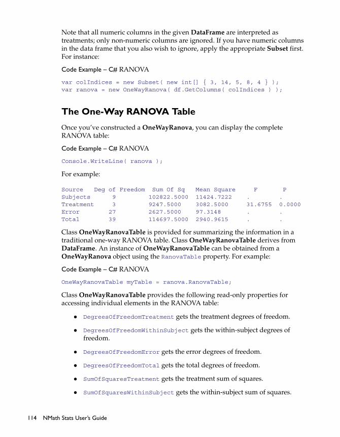
Note that all numeric columns in the given DataFrame are interpreted as treatments; only non-numeric columns are ignored. If you have numeric columns in the data frame that you also wish to ignore, apply the appropriate Subset first. For instance:
Code Example – C# RANOVA
var colIndices = new Subset( new int[] { 3, 14, 5, 8, 4 } );var ranova = new OneWayRanova( df.GetColumns( colIndices ) );
The One-Way RANOVA Table
Once you’ve constructed a OneWayRanova, you can display the complete RANOVA table:
Code Example – C# RANOVA
Console.WriteLine( ranova );
For example:
Source Deg of Freedom Sum Of Sq Mean Square F PSubjects 9 102822.5000 11424.7222 . .Treatment 3 9247.5000 3082.5000 31.6755 0.0000Error 27 2627.5000 97.3148 . .Total 39 114697.5000 2940.9615 . .
Class OneWayRanovaTable is provided for summarizing the information in a traditional one-way RANOVA table. Class OneWayRanovaTable derives from DataFrame. An instance of OneWayRanovaTable can be obtained from a OneWayRanova object using the RanovaTable property. For example:
Code Example – C# RANOVA
OneWayRanovaTable myTable = ranova.RanovaTable;
Class OneWayRanovaTable provides the following read-only properties for accessing individual elements in the RANOVA table:
DegreesOfFreedomTreatment gets the treatment degrees of freedom.
DegreesOfFreedomWithinSubject gets the within-subject degrees of freedom.
DegreesOfFreedomError gets the error degrees of freedom.
DegreesOfFreedomTotal gets the total degrees of freedom.
SumOfSquaresTreatment gets the treatment sum of squares.
SumOfSquaresWithinSubject gets the within-subject sum of squares.
114 NMath Stats User’s Guide

SumOfSquaresTotal gets the total sum of squares.
SumOfSquaresError gets the error sum of squares.
MeanSquareTreatment gets the treatment mean square.
MeanSquareWithinSubject gets the within-subject mean square.
MeanSquareError gets the error mean square.
MeanSquareTotal gets the total mean square.
FStatistic gets the F statistic for the RANOVA.
FStatisticPValue gets the p-value for the F statistic.
Grand Mean, Subject Means, and Treatment Means
Class OneWayRanova provides properties for retrieving the grand mean, subject means, and treatment means:
GrandMean gets the grand mean of the data. The grand mean is the mean of all of the data.
SubjectMeans gets a vector of means for each subject.
TreatmentMeans gets a vector of means for each treatment.
Critical Value of the F Statistic
Class OneWayRanova provides the convenience function FStatisticCriticalValue() which computes the critical value for the RANOVA F statistic at a given significance level. Thus:
Code Example – C# RANOVA
double alpha = 0.01;double critVal = ranova.FStatisticCriticalValue( alpha );
Updating One-Way RANOVA Objects
Method SetData() updates an entire repeated measures analysis of variance object with new data. As with the class constructors (see above), you can supply data as a matrix or as a data frame. For instance, this code updates a RANOVA with data from matrix A:
Code Example – C# RANOVA
ranova.SetData( A );
Chapter 8. Analysis of Variance 115

8.3 Two-Way Balanced ANOVA
Class TwoWayAnova performs a balanced two-way analysis of variance. Two-way analysis of variance is a direct extension of one-way analysis of variance (Section 8.1). In this case, data are grouped according to two factors—for example, sex and age group—rather than a single factor. The total variability is partitioned into components associated with each of the two factors, their interaction, and the residual (or error).
Creating Two-Way ANOVA Objects
A TwoWayAnova instance is constructed from data in a data frame. Three column indices are specified in the data frame: the column containing the first factor, the column containing the second factor, and the column containing the numeric data. For example, this code groups the numeric data in column 3 of DataFrame df by factors constructed from columns 0 and 4:
Code Example – C# ANOVA
var anova = new TwoWayAnova( df, 0, 4, 3 );
Factor objects are constructed from the factor columns using the DataFrame method GetFactor(), which creates a sorted array of the unique values (Section 2.10). The indicated data column must be of type DFNumericColumn.
NOTE—Class TwoWayAnova throws an InvalidArgumentException if the data contains missing values (NaNs).
The Two-Way ANOVA Table
Once you’ve constructed a TwoWayAnova, you can display the complete ANOVA table:
Code Example – C# ANOVA
Console.WriteLine( anova );
For example:
Source Deg of Freedom SumOfSq Mean Square F PFactorA 1 1782.0450 1782.0450 14.2121 0.0008FactorB 1 2838.8113 2838.8113 22.6399 0.0001Interaction 1 108.0450 108.0450 0.8617 0.3612Error 28 3510.9075 125.3896 . .Total 31 8239.8088 . . .
Class TwoWayAnovaTable is provided for summarizing the information in a traditional two-way ANOVA table. Class TwoWayAnovaTable derives from
116 NMath Stats User’s Guide

DataFrame. An instance of TwoWayAnovaTable can be obtained from a TwoWayAnova object using the AnovaTable property. For example:
Code Example – C# ANOVA
TwoWayAnovaTable myTable = anova.AnovaTable;
Class TwoWayAnovaTable provides the following member functions and read-only properties for accessing individual elements in the ANOVA table:
DegreesOfFreedom() gets the degrees of freedom for a specified factor.
ErrorDegreesOfFreedom gets the number of degrees of freedom for the error.
InteractionDegreesOfFreedom gets the number of degrees of freedom for the interactions.
TotalDegreesOfFreedom gets the total number of degrees of freedom.
SumOfSquares() gets the sum of squares for a specified factor.
InteractionSumOfSquares gets the sum of squares for the interaction.
ErrorSumOfSquares gets the sum of squares for the error.
TotalSumOfSquares gets the total sum of squares.
MeanSquare() gets the mean square for a specified factor.
InteractionMeanSquare gets the mean square for the interaction.
ErrorMeanSquare gets the mean square for the error.
Fstatistic() gets the F statistic for a specified factor.
InteractionFstatistic gets the F statistic for the interaction.
FstatisticPvalue() gets the p-value for the F statistic for a specified factor.
InteractionFstatisticPvalue gets the p-value for the F statistic for the interaction.
Factors are identified to accessor methods by name, which corresponds to the name of the column in the original data frame that was used to create the Factor. For instance, if one factor in the ANOVA is named Dosage, this code gets the F statistic and p-value for that factor:
Code Example – C# ANOVA
double Fstatistic = anova.AnovaTable.Fstatistic( “Dosage” );double Pvalue = anova.AnovaTable.FstatisticPvalue( “Dosage” );
Chapter 8. Analysis of Variance 117

Cell Data
Class TwoWayAnova provides the GetCellData() method for accessing the data in a cell, as defined by a specified level of each of the factors in the ANOVA. For example, if anova has factor Sex with levels Male and Female, and factor AgeGroup with levels Child, Adult, and Senior, this code gets the data for adult females:
Code Example – C# ANOVA
DFNumericColumn data = anova.GetCellData( “Sex”, “Female”, “AgeGroup”, “Adult” );
A copy of the data is returned as a DFNumericColumn object.
Grand Mean, Cell Means, and Group Means
Class TwoWayAnova provides the following properties and member functions for accessing the grand mean, cell means, and group means:
GrandMean gets the grand mean. The grand mean is the mean of all the data.
GetMeanForCell() returns the mean for a specified cell.
GetMeanForFactorLevel() returns the mean for a specified factor level.
Again, factors and factor levels are identified to accessor methods by name. For example, if anova has factor Sex with levels Male and Female, and factor AgeGroup with levels Child, Adult, and Senior, this code gets the mean for all males:
Code Example – C# ANOVA
double meanM = anova.GetMeanForFactorLevel( “Sex”, “Male” );
This code gets the mean for male children:
Code Example – C# ANOVA
double meanMChild = anova.GetMeanForCell( “Sex”, “Male”, “AgeGroup”, “Child” );
ANOVA Regression Parameters
NMath Stats solves the two-way ANOVA problem using multiple linear regression. If all you wish to know is the information in the standard ANOVA table, you can safely ignore the regression details, but properties and member functions are provided for retrieving information about the underlying regression parameters.
118 NMath Stats User’s Guide
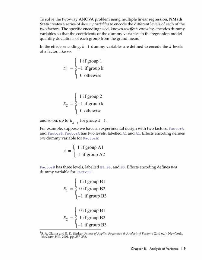
To solve the two-way ANOVA problem using multiple linear regression, NMath Stats creates a series of dummy variables to encode the different levels of each of the two factors. The specific encoding used, known as effects encoding, encodes dummy variables so that the coefficients of the dummy variables in the regression model quantify deviations of each group from the grand mean.1
In the effects encoding, dummy variables are defined to encode the levels of a factor, like so:
and so on, up to for group .
For example, suppose we have an experimental design with two factors: FactorA and FactorB. FactorA has two levels, labelled A1 and A1. Effects encoding defines one dummy variable for FactorA:
FactorB has three levels, labelled B1, B2, and B3. Effects encoding defines two dummy variable for FactorB:
1S. A. Glantz and B. K. Slinker, Primer of Applied Regression & Analysis of Variance (2nd ed.), NewYork, McGraw-Hill, 2001, pp. 357-358.
k 1– k
E1
1 if group 1
1– if group k
0 othewise
=
E2
1 if group 2
1– if group k
0 othewise
=
Ek 1–k 1–
A1 if group A1
1– if group A2
=
B1
1 if group B1
0 if group B2
1 if group B3–
=
B2
0 if group B1
1 if group B2
1 if group B3–
=
Chapter 8. Analysis of Variance 119

Combined, these three dummy variables completely identify all the combinations of FactorA and FactorB. The multiple regression model is then:
where
the intercept is an estimate of the grand mean
estimates the difference between the grand mean and the mean of A1
is the difference between the grand mean and the mean of A2
estimates the difference between the grand mean and the mean of B1
estimates the difference between the grand mean and the mean of B2
estimates the difference between the grand mean and the mean of B3
NMath Stats includes several classes that derive from LinearRegressionParameter, and provide access to the dummy variable regression parameters in an ANOVA analysis of variance:
Class AnovaRegressionParameter provides a SumOfSquares property that gets the sum of squares due to a parameter.
Class AnovaRegressionFactorParam derives from AnovaRegressionParameter and provides the additional properties FactorName, which gets the name of the ANOVA factor encoded by a dummy variable, FactorLevel, which gets the level of the ANOVA factor encoded by a dummy variable, and Encoding, which gets the actual encoding. The encoding is the value the dummy variable assumes when an ANOVA observation is made with the factor at that level.
Class AnovaRegressionInteractionParam also derives from AnovaRegressionParameter and provides the additional properties FactorAName and FactorALevel, which get the name and level of the first factor in the interaction, and FactorBName and FactorBLevel, which get the name and level of the second factor in the interaction.
Of course, these classes also inherit from LinearRegressionParameter methods such as TStatisticPValue(), TStatistic(), TStatisticCriticalValue(), and ConfidenceInterval() for testing statistical hypotheses regarding parameter values in a linear regression (Section 6.5).
Instances of these classes cannot be constructed independently. Instead, they are returned by properties and member functions on class TwoWayAnova:
RegressionInterceptParameter gets the intercept parameter in the linear regression as an AnovaRegressionParameter.
A b0 bAA bB1B1 bB2
B2 bAB1AB1 bAB2
AB2+ + + + +=
b0
bA
bA–
bB11
bB21
bB1bB2
+ –
120 NMath Stats User’s Guide

GetRegressionFactorParameter() returns the AnovaRegressionFactorParam associated with a specified factor level.
RegressionFactorParameters gets a complete array of AnovaRegressionFactorParam estimates for the different factor levels.
GetRegressionInteractionParameter() returns the AnovaRegressionInteractionParam associated with the specified interaction.
RegressionInteractionParameters gets a complete array of AnovaRegressionInteractionParam estimates for the interactions.
For example, this code gets the regression parameter for FactorA at level A1:
Code Example – C# ANOVA
AnovaRegressionFactorParam param anova.GetRegressionFactorParameter( "FactorA", "A1" );Console.WriteLine( param );
Example output:
Value : 4.375Standard Error : 1.63741694728596t-Statistic for parameter = 0 : 2.67189124141632p-value for t-Statistic : 0.01555167846501360.05 confidence interval : [9.3491E-001, 7.8151E+000]
Note that method GetRegressionFactorParameter() may return null. In the effects encoding method, there are dummy variables defined to encode the levels of a factor. Hence, one level does not have a dummy variable associated with it in the linear regression, and a null reference may be returned even though a valid factor level is specified. Thus:
Code Example – C# ANOVA
AnovaRegressionFactorParam param = anova.GetRegressionFactorParameter( "FactorA", "A2" );// param == null
Similarly, method GetRegressionInteractionParameter() may return null. If there are different levels for the first factor and different levels for the second factor, there are dummy variables corresponding to the interactions. Hence, some interactions do not have a dummy variable associated with them in the linear regression, and a null reference may be returned even though valid interactions are specified.
This code prints out the intercept regression parameter, all factor regression parameters, and all interaction regression parameters:
k 1– k
j kj 1– k 1–
Chapter 8. Analysis of Variance 121

Code Example – C# ANOVA
Console.WriteLine( "Intercept" );Console.WriteLine( anova.RegressionInterceptParameter );Console.WriteLine();
AnovaRegressionFactorParam[] factorParams = anova.RegressionFactorParameters;for ( int i = 0; i < factorParams.Length; i++ ){ Console.WriteLine( factorParams[i].FactorLevel ); Console.WriteLine( factorParams[i] ); Console.WriteLine();}
AnovaRegressionInteractionParam[] interactionParams = anova.RegressionInteractionParameters;for ( int i = 0; i < interactionParams.Length; i++ ){ Console.WriteLine( interactionParams[i].FactorALevel + " x " + interactionParams[i].FactorBLevel ); Console.WriteLine( interactionParams[i] ); Console.WriteLine();}
Example output:
InterceptValue : 28.875Standard Error : 1.63741694728596t-Statistic for parameter = 0: 17.6344821933477p-value for t-Statistic : 8.35997937542743E-130.05 confidence interval : [2.5435E+001, 3.2315E+001]
A1Value : 4.375Standard Error : 1.63741694728596t-Statistic for parameter = 0: 2.67189124141632p-value for t-Statistic : 0.01555167846501360.05 confidence interval : [9.3491E-001, 7.8151E+000]
B1Value : 25.5Standard Error : 2.31565725411135t-Statistic for parameter = 0: 11.0119923640365p-value for t-Statistic : 1.98637151171965E-090.05 confidence interval : [2.0635E+001, 3.0365E+001]
122 NMath Stats User’s Guide

B2Value : -7.25Standard Error : 2.31565725411135t-Statistic for parameter = 0: -3.13086057408882p-value for t-Statistic : 0.005775634746369330.05 confidence interval : [-1.2115E+001, -2.3850E+000]
A1 x B1Value : 6Standard Error : 2.31565725411135t-Statistic for parameter = 0: 2.59105702683213p-value for t-Statistic : 0.01844271589090040.05 confidence interval : [1.1350E+000, 1.0865E+001]
A1 x B2Value : -0.999999999999999Standard Error : 2.31565725411135t-Statistic for parameter = 0: -0.431842837805354p-value for t-Statistic : 0.6709841112336030.05 confidence interval : [-5.8650E+000, 3.8650E+000]
8.4 Two-Way Unbalanced ANOVA
Class TwoWayAnovaUnbalanced is the base class for performing a two-way ANOVA when the number of observations in each cell is not the same—an unbalanced design. Three derived classes are provided:
TwoWayAnovaTypeI performs a Type I ANOVA on unbalanced data. Type I, also called sequential sum of squares, tests the main effect of factor A, followed by the main effect of factor B after the main effect of A, followed by the interaction effect AB after the main effects.
TwoWayAnovaTypeII performs a Type II ANOVA on unbalanced data. This type tests for each main effect after the other main effect. No significant interaction is assumed.
TwoWayAnovaTypeIII performs a Type III ANOVA on unbalanced data. This type tests for the presence of a main effect after the other main effect and interaction.
For more information on the different ways to calculate the sums of squares for ANOVA, see
http://goanna.cs.rmit.edu.au/~fscholer/anova.php
Chapter 8. Analysis of Variance 123

Creating UnbalancedTwo-Way ANOVA Objects
Unbalanced two-way ANOVA instances are constructed in the same manner as balanced TwoWayAnova objects (Section 8.3). For example, this code groups the numeric data in column 3 of DataFrame df by factors constructed from columns 0 and 1:
Code Example – C# Unbalanced ANOVA
var type1anova = new TwoWayAnovaTypeI( df, 0, 1, 2 );
Unbalanced Two-Way ANOVA Tables and Regression Parameters
Using an unbalanced two-way ANOVA object is similar to using a balanced TwoWayAnova object (Section 8.3). For instance, this code prints the ANOVA table.
Code Example – C# Unbalanced ANOVA
Console.WriteLine( type1anova.AnovaTable );
This code prints the regression parameters.
Code Example – C# Unbalanced ANOVA
Console.WriteLine( "FACTOR A ANOVA --------" );var fa = type1anova.FactorARegressionFactorParameters;for ( int i = 0; i < fa.Length; i++ ){ Console.WriteLine( fa[i] ); Console.WriteLine();}
Console.WriteLine( "\nFACTOR B ANOVA --------" );var fb = type1anova.FactorBRegressionFactorParameters;for ( int i = 0; i < fb.Length; i++ ){ Console.WriteLine( fb[i] ); Console.WriteLine();}
Console.WriteLine( "\nINTERACTION FACTOR ANOVA --------" );var fi = type2anova.InteractionRegressionFactorParameters;for ( int i = 0; i < fi.Length; i++ ){ Console.WriteLine( fi[i] ); Console.WriteLine();}
124 NMath Stats User’s Guide
8.5 Two-Way Repeated Measures ANOVA
NMath Stats provides two classes for calculating a two-way analysis of variance with repeated measures (RANOVA):
Class TwoWayRanova performs a balanced two-way analysis of variance with repeated measures on one factor.
Class TwoWayRanovaTwo performs a balanced two-way analysis of variance with repeated measures on both factors.
Both classes extend TwoWayAnova, and so inherit the methods and properties described in Section 8.3. Like TwoWayAnova, both TwoWayRanova and TwoWayRanovaTwo use multiple linear regression to compute the RANOVA values.
Creating Two-Way RANOVA Objects
Instances of both TwoWayRanova and TwoWayRanovaTwo are constructed from data in a data frame. Three column indices are specified in the data frame: the column containing the first factor, the column containing the second factor, and the column containing the numeric data. For TwoWayRanova, the first factor is the repeated factor; for TwoWayRanovaTwo, both factors are repeated.
For example, this code groups the numeric data in column 3 of DataFrame df by factors constructed from columns 0 and 4:
Code Example – C# RANOVA
var ranova = new TwoWayRanova( df, 0, 4, 3 );
The factor constructed from column 0 is the repeated factor. In the following example, both factors are repeated:
Code Example – C# RANOVA
var ranova2 = new TwoWayRanovaTwo( df, 0, 4, 3 );
NOTE—Both TwoWayRanova and TwoWayRanovaTwo throw an InvalidArgumentEx-ception if the data contains missing values (NaNs).
Two-Way RANOVA Tables
Once you’ve constructed a TwoWayRanova, you can display the complete RANOVA table:
Code Example – C# RANOVA
var ranova = new TwoWayRanova( df, 0, 4, 3 );
Chapter 8. Analysis of Variance 125

Console.WriteLine( ranova );
For instance:
Source Deg of Freedom SumOfSqu Mean Square F PFactorA 1 0.2032 0.2032 29.2322 0.0001Subjects 14 1.7559 0.1254 . .FactorB 1 0.0205 0.0205 0.1635 0.6921Interaction 1 0.0830 0.0830 11.9442 0.0039Error 14 0.0973 0.0070 . .Total 31 2.1599 . . .
Class TwoWayRanovaTable summarizes the information in a traditional two-way RANOVA table with repeated measures on one factor. An instance of TwoWayRanovaTable can be obtained from a TwoWayRanova object using the RanovaTable property. For example:
Code Example – C# RANOVA
TwoWayRanovaTable myTable = ranova.RanovaTable;
Class TwoWayRanovaTable derives from TwoWayAnovaTable, and so inherits the properties described in Section 8.3. In addition, TwoWayRanovaTable provides the following properties for accessing the new row in the RANOVA table for repeated measures on one factor:
SubjectsDegreesOfFreedom gets the subjects degrees of freedom.
SubjectsSumOfSquares gets the sum of squares for the subjects.
SubjectsMeanSquare gets the mean square for the subjects.
Similarly, once you’ve constructed a TwoWayRanovaTwo, you can display the RANOVA table:
Code Example – C# RANOVA
var ranova2 = new TwoWayRanovaTwo( df, 0, 4, 3 );Console.WriteLine( ranova2 );
For example:
Source Deg of Freedom SumOfSq Mean Square F PFactorA 1 1.4700 1.4700 88.2000 0.0000FactorB 2 14.5654 7.2827 59.2348 0.0000Interaction 2 3.3387 1.6694 18.9305 0.0001A x Subject 14 1.7213 0.1229 . .B x Subject 7 0.1167 0.0167 . .Error 14 1.2346 0.0882 . .Total 47 29.3592 . . .
126 NMath Stats User’s Guide

An instance of TwoWayRanovaTwoTable can be obtained from a TwoWayRanovaTwo object using the RanovaTable property. For example:
Code Example – C# RANOVA
TwoWayRanovaTwoTable myTable = ranova2.RanovaTable;
Class TwoWayRanovaTwoTable also derives from TwoWayAnovaTable, and provides the following methods for accessing the additional rows in the RANOVA table with repeated measures on both factors:
SubjectInteractionDegreesOfFreedom() returns the degrees of freedom for the interaction between subjects and the specified factor.
SubjectInteractionSumOfSquares() returns the sum of squares for the interaction between subjects and the specified factor.
SubjectInteractionMeanSquare returns the mean square for the interaction between subjects and the specified factor.
Chapter 8. Analysis of Variance 127

128 NMath Stats User’s Guide

CHAPTER 9. NON-PARAMETRIC TESTS
Non-parametric (or distribution-free) tests make no assumptions about the probability distributions of the variables being assessed. NMath Stats provides classes for several common non-parametric tests:
Class OneSampleKSTest performs a Kolmogorov-Smirnov test of the distribution of one sample.
Class TwoSampleKSTest performs a two-sample Kolmogorov-Smirnov test to compare the distributions of values in two data sets.
Class ShapiroWilkTest tests the null hypothesis that the sample comes from a normally distributed population.
Class OneSampleAndersonDarlingTest performs a Anderson-Darling test of the distribution of one sample.
Class KruskalWallisTest performs a Kruskal-Wallis rank sum test.
This chapter describes the non-parametric test classes.
See Section 3.9 for Spearman’s rank correlation coefficient, commonly known as Spearman’s rho.
9.1 One Sample Kolmogorov-Smirnov Test
Class OneSampleKSTest performs a Kolmogorov-Smirnov test of the distribution of one sample. This class compares the distribution of a given sample to the hypothesized distribution defined by a specified cumulative distribution function (CDF). For each potential value x, the Kolmogorov-Smirnov test compares the proportion of values less than x with the expected number predicted by the specified CDF. The null hypothesis is that the given sample data follow the specified distribution. The alternative hypothesis that the data do not have that distribution.
Chapter 9. Non-Parametric Tests 129
Sample data can be passed to the constructor as a vector, numeric column in a data frame, or an array of doubles. The hypothesized distribution can be specified either by using an instance of ProbabilityDistribution or by supplying a delegate that encapsulates the CDF of the hypothesized distribution. For example, this code creates a OneSampleKSTest instance that compares the distribution of data to a standard normal distribution:
Code Example – C# Kolmogorov-Smirnov test
var norm = new NormalDistribution();var ks = new OneSampleKSTest( data, norm );
If myDist.CDF() is the CDF for some distribution, this code creates a OneSampleKSTest instance that compares the distribution of the data in column 3 of DataFrame df to the hypothesized distribution:
Code Example – C# Kolmogorov-Smirnov test
var ks = new OneSampleKSTest( df[3], new Func<double, double>(myDist.CDF) );
By default, a OneSampleKSTest object performs the Kolmogorov-Smirnov test with . A different alpha level can be specified at the time of construction using constructor overloads, or after construction using the provided Alpha property.
Once you’ve constructed and configured a OneSampleKSTest object, you can access the various test results using the provided properties:
Code Example – C# Kolmogorov-Smirnov test
Console.WriteLine( "statistic = " + test.Statistic );Console.WriteLine( "p-value = " + test.P );Console.WriteLine( “alpha = “ + test.Alpha );Console.WriteLine( "reject the null hypothesis? " + test.Reject);
9.2 Two Sample Kolmogorov-Smirnov Test
Class TwoSampleKSTest performs a two-sample Kolmogorov-Smirnov test to compare the distributions of values in two data sets. For each potential value x, the Kolmogorov-Smirnov test compares the proportion of values in the first sample less than x with the proportion of values in the second sample less than x. The null hypothesis is that the two samples have the same continuous distribution. The alternative hypothesis is that they have different continuous distributions.
0.01=
130 NMath Stats User’s Guide

Sample data can be passed to the constructor as vectors, numeric columns in a data frame, or arrays of doubles. Thus:
Code Example – C# Kolmogorov-Smirnov test
var ks = new TwoSampleKSTest( data1, data2 );
By default, a TwoSampleKSTest object performs the Kolmogorov-Smirnov test with . A different alpha level can be specified at the time of construction using constructor overloads, or after construction using the provided Alpha property.
Once you’ve constructed and configured a TwoSampleKSTest object, you can access the various test results using the provided properties:
Code Example – C# Kolmogorov-Smirnov test
Console.WriteLine( "statistic = " + test.Statistic );Console.WriteLine( "p-value = " + test.P );Console.WriteLine( “alpha = “ + test.Alpha );Console.WriteLine( "reject the null hypothesis? " + test.Reject);
9.3 Shapiro-Wilk Test
Class ShapiroWilkTest tests the null hypothesis that a sample comes from a normally distributed population. The sample data provided must be of size between 3 and 5000. If the size becomes too large, then the test begins to perform poorly.
Code Example – C# Shapiro-Wilk test
var data = new DoubleVector( "4.6057571 5.0352571 2.5780990 3.8300667 3.9096730 0.3203129 " + "0.7165054 9.8681061 3.8967762 9.4639023 6.4092569 2.9835816 " + "8.1763496 8.5650066 10.2810477 7.7123572 2.6411587 2.5043797 " + "7.5617508 11.2223571" );
double alpha = 0.1;var test = new ShapiroWilkTest( data, alpha );
Once you’ve constructed and configured a TwoSampleKSTest object, you can access the various test results using the provided properties:
Code Example – C# Shapiro-Wilk test
Console.WriteLine( "statistic = " + test.Statistic );Console.WriteLine( "p-value = " + test.P );Console.WriteLine( “alpha = “ + test.Alpha );Console.WriteLine( "reject the null hypothesis? " + test.Reject);
0.01=
Chapter 9. Non-Parametric Tests 131

9.4 One Sample Anderson-Darling Test
Class OneSampleAndersonDarlingTest performs a Anderson-Darling test of the distribution of one sample. An Anderson-Darling test compares the distribution of a given sample to normal distribution function (CDF). The alternative hypothesis that the data do not have a normal distribution.
Code Example – C# Anderson-Darling test
int n = 100;DoubleVector data = new DoubleVector( n, new RandGenGamma( 23.0 ) );OneSampleAndersonDarlingTest test = new OneSampleAndersonDarlingTest( data );
Console.WriteLine( "statistic = " + test.Statistic );Console.WriteLine( "p-value = " + test.P );Console.WriteLine( “alpha = “ + test.Alpha );Console.WriteLine( "reject the null hypothesis? " + test.Reject);
9.5 Kruskal-Wallis Test
Class KruskalWallisTest performs a Kruskal-Wallis rank sum test. The Kruskal-Wallis test is a non-parametric test for equality of population medians among groups. It is a non-parametric version of the classical one-way ANOVA. The interface for KruskalWallisTest is nearly identical to OneWayAnova.
Creating Kruskal-Wallis Objects
A KruskalWallisTest instance is constructed from numeric data organized into different groups. The groups need not contain the same number of observations. For example, this code constructs a KruskalWallisTest from an array of DoubleVector objects. Each vector in the array contains data for a single group:
Code Example – C# Kruskal-Wallis test
var a = new DoubleVector(6.4, 6.8, 7.2, 8.3, 8.4, 9.1, 9.4, 9.7);var b = new DoubleVector(2.5, 3.7, 4.9, 5.4, 5.9, 8.1, 8.2);var c = new DoubleVector(1.3, 4.1, 4.9, 5.2, 5.5, 8.2);
var data_ = new DoubleVector[] { a, b, c };
132 NMath Stats User’s Guide

var test = new KruskalWallisTest( data_);
An optional boolean parameter may also be supplied to the constructor. If true, a standard correction for ties is applied.
Code Example – C# Kruskal-Wallis test
bool correct_for_ties = true;var test = new KruskalWallisTest( data, correct_for_ties_);
This correction usually makes little difference in the value of the test statistic, unless there are a large number of ties.
This code constructs a KruskalWallisTest from a data frame df:
Code Example – C# Kruskal-Wallis test
var test = new KruskalWallisTest( df, 1, 3 );
Two column indices are also provided: a group column and a data column. A Factor is constructed from the group column using the DataFrame method GetFactor(), which creates a sorted array of the unique values. The specified data column must be of type DFNumericColumn.
Lastly, you can also construct a KruskalWallisTest from a DoubleMatrix:
Code Example – C# Kruskal-Wallis test
var data = new DoubleMatrix( "6 x 5 [ 24 14 11 7 19 15 7 9 7 24 21 12 7 7 19 27 17 13 12 15 33 14 12 12 10 23 16 18 18 20 ]" );
bool correct_for_ties = true;var test = new KruskalWallisTest( data, correct_for_ties );
Each column in the given matrix contains the data for a group. If your groups have different numbers of observations, you must pad the columns with Double.NaN values until they are all the same length, because a DoubleMatrix must be rectangular. Alternatively, use one of the other constructors described above.
The Kruskal-Wallis Table
Once you’ve constructed a KruskalWallisTest, you can display the complete results table:
Code Example – C# Kruskal-Wallis test
Console.WriteLine( test );
Chapter 9. Non-Parametric Tests 133

For example:
Source Deg of Freedom Sum Of Sq Mean Sq Chi-sq PBetween groups 2 13.5000 6.7500 0.7714 0.6800Within groups 11 214 19.4545 . .Total 13 227.5000 . . .
Class KruskalWallisTable is provided for summarizing the information in the results table. Class KruskalWallisTable derives from DataFrame. An instance of KruskalWallisTable can be obtained from a KruskalWallisTest object using the Table property. For example:
Code Example – C# Kruskal-Wallis test
KruskalWallisTable table = test.able;
Class KruskalWallisTable provides the following read-only properties for accessing individual elements in the results table:
DegreesOfFreedomBetween gets the between-groups degrees of freedom.
DegreesOfFreedomWithin gets the within-groups degrees of freedom.
DegreesOfFreedomTotal gets the total degrees of freedom.
SumOfSquaresBetween gets the between-groups sum of squares.
SumOfSquaresWithin gets the within-groups sum of squares.
SumOfSquaresTotal gets the total sum of squares.
MeanSquareBetween gets the between-groups mean square. The between-groups mean square is the between-groups sum of squares divided by the between-groups degrees of freedom.
MeanSquareWithin gets the within-group mean square. The within-groups mean square is the within-group sum of squares divided by the within-group degrees of freedom.
MeanSquareTotal gets the total mean square. The total mean square is the total sum of squares divided by the total degrees of freedom.
Statistic gets the test statistic.
PValue gets the p-value for the test statistic.
134 NMath Stats User’s Guide

Ranks, Grand Mean Ranks, Group Means Ranks, and Group Sizes
Class KruskalWallisTest provides properties and methods for retrieving the ranks, grand mean ranks, group means ranks, and group sizes:
Ranks gets an array of vectors containing the ranks of the data.
GrandMeanRank gets the grand mean rank of the data. The grand mean rank is the mean of all of the data ranks.
GroupMeanRanks gets a vector of group mean ranks.
GroupSizes gets an array of group sizes.
GroupNames gets an array of group names. If the test was constructed from a data frame using a grouping column, the group names are the sorted, unique Factor levels created from the column values. If the test object was constructed from a matrix or an array of vectors, the group names are simply Group_0, Group_1...Group_n.
GetGroupRanks() returns the ranks for a specified group, identified either by group name or group number (a zero-based index into the Ranks array).
GetGroupMeanRank() returns the mean rank for a specified group, identified either by group name or group number (a zero-based index into the GroupMeanRanks vector).
GetGroupSize() returns the mean for a specified group, identified either by group name or group number (a zero-based index into the GroupSizes array).
For example, if a KruskalWallisTest is constructed from a matrix, this code returns the mean rank for the group in the third column of the matrix:
Code Example – C# Kruskal-Wallis test
double mean = test.GetGroupMeanRank( 2 );
If a KruskalWallisTest is constructed from a data frame using a grouping column with values male and female, this code returns the mean rank for the male group:
Code Example – C# Kruskal-Wallis test
double maleMean = test.GetGroupMeanRank( “male” );
Chapter 9. Non-Parametric Tests 135

Critical Value of the Test Statistic
Class KruskalWallisTest provides the convenience function StatisticCriticalValue() which computes the critical value for the test statistic at a given significance level. Thus:
Code Example – C# Kruskal-Wallis test
double alpha = 0.05;double critVal = test.StatisticCriticalValue( alpha );
Updating Kruskal-Wallis Test Objects
Method SetData() updates an entire test object with new data. As with the class constructors (see above), you can supply data as an array of group vectors, a matrix, or as a data frame. For instance, this code updates a test with data from DataFrame df, using column 2 as the group column and column 5 as the data column:
Code Example – C# Kruskal-Wallis test
test.SetData( df, 2, 5 );
136 NMath Stats User’s Guide

CHAPTER 10. MULTIVARIATE TECHNIQUES
Multivariate statistical analysis techniques are useful when you need a concise understanding of large amounts of data. NMath Stats provides classes for dimension reduction using principal component analysis or factor analysis, and case reduction using hierarchical cluster analysis and k-means clustering.
This chapter describes the multivariate statistical analysis classes.
10.1 Principal Component Analysis
Principal component analysis (PCA) finds a smaller set of synthetic variables that capture the variance in an original data set. The first principal component accounts for as much of the variability in the data as possible, and each succeeding orthogonal component accounts for as much of the remaining variability as possible. In NMath Stats, classes DoublePCA and FloatPCA perform principal component analyses.
Creating Principal Component Analyses
A DoublePCA or FloatPCA instance is constructed from a matrix or a dataframe containing numeric data. Each column represents a variable, and each row represents an observation:
Code Example – C# principal component analysis (PCA)
var pca = new DoublePCA( data );
The data may optionally be zero-centered and scaled to have unit variance:
Code Example – C# principal component analysis (PCA)
bool center = true;bool scale = true;var pca = new DoublePCA( data, center, scale );
By default, variables are centered but not scaled.
Chapter 10. Multivariate Techniques 137

After construction, you can retrieve information about the data set using the provided read-only properties:
Data gets the data matrix. If centering or scaling were specified at construction time, the returned matrix may not match the original data.
NumberOfObservations gets the number of observations in the data matrix.
NumberOfVariables gets the number of variables in the data matrix.
IsCentered returns true if the data supplied at construction time was shifted to be zero-centered.
IsScaled returns true if the data supplied at construction time was scaled to have unit variance.
Means gets the column means of the data matrix. If centering is specified, the column means are substracted from the column values before analysis takes place.
Norms gets the column norms (1-norm). If scaling is specified, column values are scaled to have unit variance before analysis by dividing by the column norm.
Principal Component Analysis Results
The Loadings property gets the complete loading matrix. Each column in the loading matrix is a principal component. The first principal component accounts for as much of the variability in the data as possible, and each succeeding orthogonal component accounts for as much of the remaining variability as possible.
Code Example – C# principal component analysis (PCA)
Console.WriteLine( "Loading Martrix = " + pca.Loadings );
The provided indexer also gets a specified principal component, referenced by zero-based index. For example:
Code Example – C# principal component analysis (PCA)
Console.WriteLine( "First principal component = " + pca[0] );Console.WriteLine( "Second principal component = " + pca[1] );
The VarianceProportions property gets an ordered vector containing the proportion of the total variance accounted for by each principal component. CumulativeVarianceProportions gets the cumulative variance proportions. Thus:
138 NMath Stats User’s Guide

Code Example – C# principal component analysis (PCA)
Console.WriteLine( "Variance Proportions = " + pca.VarianceProportions ); Console.WriteLine( "Cumulative Variance Proportions = " + pca.CumulativeVarianceProportions );
The Threshold() method calculates the number of principal components required to account for a given proportion of the total variance:
Code Example – C# principal component analysis (PCA)
Console.WriteLine( "PCs that account for 99% of the variance = " + pca.Threshold( .99 ) );
The StandardDeviations property gets the standard deviations of the principal components. Eigenvalues gets the eigenvalues of the covariance/correlation matrix, though the calculation is actually performed using the singular values of the data matrix. The eigenvalues of the covariance/correlation matrix are equal to the squares of the standard deviations of the principal components.
Lastly, the Scores property gets the score matrix. The scores are the data formed by transforming the original data into the space of the principal components:
Code Example – C# principal component analysis (PCA)
Console.WriteLine( "Scores = " + pca.Scores );
This code displays the data in the minimal synthetic dimensions required to account for 99% of the variance:
Code Example – C# principal component analysis (PCA)
Slice rowSlice = Slice.All;var colSlice = new Slice( 0, pca.Threshold( .99 ) );Console.WriteLine( pca.Scores[ rowSlice, colSlice ] );
10.2 Factor Analysis
Factor analysis describes the variability among observed, correlated variables in terms of a potentially lower number of unobserved variables, called factors.
In general, factor analysis consists of two steps:
In the extraction step, factors are extracted from the data.
In NMath Stats, IFactorExtraction is the interface for factor extraction algo-rithms. Class PCFactorExtraction implements the principle component (PC) algorithm for factor extraction.
Chapter 10. Multivariate Techniques 139
In the rotation step, the factors are rotated in order to maximize the relationship between the variables and the factors.
In NMath Stats, IFactorRotation is the interface for factor rotation algo-rithms. Class VarimaxRotation computes the varimax rotation of the factors. Factors are rotated to maximize the sum of the variances of the squared loadings. Kaiser normalization is optionally performed. Class NoRotation can be used when no rotation is desired.
Creating Factor Analyses
NMath Stats provides three classes for performing factor analysis:
FactorAnalysisCorrelation performs a factor analysis on given case data by forming the correlation matrix for the variables.
FactorAnalysisCovariance performs a factor analysis on given case data using the covariance matrix.
DoubleFactorAnalysis performs a factor analysis on a symmetric matrix of data, assumed to be either a correlation or covariance matrix, if you don’t have access to the original case data.
When case data is used, the data should provided in matrix form—the variable values in columns and each row representing a case.
All factor analysis are templatized on the extraction and rotation algorithm to use. For example:
Code Example – C# factor analysis
var fa = new FactorAnalysisCorrelation<PCFactorExtraction, VarimaxRotation>( data );
For greater control, construct the extraction and rotation objects explicitly. For example, a PCFactorExtraction instance can be constructed from a delegate for determining the number of factors to extract. The type of this argument is Func<DoubleVector, DoubleMatrix, int>. It takes as arguments the vector of eigenvalues and the matrix of eigenvectors, and returns the number of factors to extract. Class NumberOfFactors contains static methods for creating functors for several common strategies. This code extracts factors whose eigenvalues are greater than 1.2 times the mean of the eigenvalues:
Code Example – C# factor analysis
var factorExtraction = new PCFactorExtraction( NumberOfFactors.EigenvaluesGreaterThanMean( 1.2 ) );
The following code constructs a VarimaxRotation instance with a specified tolerance. Iteration stops when the relative change in the sum of the singular
140 NMath Stats User’s Guide

values is less than this number. We also specify that we do not want Kaiser normalization to be performed.
Code Example – C# factor analysis
var factorRotation = new VarimaxRotation{ Tolerance = 1e-6, Normalize = false};
Once you’ve constructed your extraction and rotation objects, you can construct the factor analysis instance:
Code Example – C# factor analysis
var fa = new FactorAnalysisCovariance<PCFactorExtraction, VarimaxRotation>( data, BiasType.Biased, factorExtraction, factorRotation );
Factor Analysis Results
Once you’ve constructed a factor analysis instance, you can access the results using the following properties:
NumberOfFactors get the number of factors extracted.
Factors gets the extracted factors. Each column of the matrix is a factor.
RotatedFactors gets the rotated factors. Each column of the matrix is a factor.
VarianceProportions gets a vector of proportion of variance explained by each factor.
CumulativeVarianceProportions gets the cumulative variance proportions.
ExtractedCommunalities get the proportion of each variable's variance that can be explained by the extracted factors jointly.
InitialCommunalities get the proportion of each variable's variance that can be explained by the factors jointly.
SumOfSquaredLoadings gets the sum of squared loadings for each extracted factor.
RotatedSumOfSquaredLoadings gets the sum of squared loadings for each rotated extracted factor.
Chapter 10. Multivariate Techniques 141

For instance:
Code Example – C# factor analysis
DoubleVector extractedCommunalities = fa.ExtractedCommunalities;for ( int i = 0; i < data.Cols; i++ ){ Console.WriteLine( "{0}\t{1}", data[i].Name, extractedCommunalities[i] );}Console.WriteLine();
for ( int i = 0; i < fa.VarianceProportions.Length; i++ ){ double varProportion = fa.VarianceProportions[i] * 100.0; double cummlativeVarProportion = fa.CumulativeVarianceProportions[i] * 100.0; double eigenValue = fa.FactorExtraction.Eigenvalues[i]; Console.WriteLine( "{0}\t\t{1}\t{2}\t\t{3}", i, eigenValue, varProportion, cummlativeVarProportion );}Console.WriteLine();
double eigenValueSum = NMathFunctions.Sum( fa.FactorExtraction.Eigenvalues );DoubleVector RotatedSSLoadingsVarianceProportions = fa.RotatedSumOfSquaredLoadings / eigenValueSum;Console.WriteLine( "\nRotated Extraction Sums of Squared Loadings - " );Console.WriteLine( "factor\tTotal\t% of Variance\tCummlative %" );Console.WriteLine( "----------------------------------------------------" );double cummlative = 0;
for ( int i = 0; i < fa.NumberOfFactors; i++ ){ double varProportion = RotatedSSLoadingsVarianceProportions[i] * 100.0; cummlative += RotatedSSLoadingsVarianceProportions[i]; double cummlativeVarProportion = cummlative * 100.0; double sumSquaredLoading = fa.RotatedSumOfSquaredLoadings[i]; Console.WriteLine( "{0}\t\t{1}\t{2}\t\t{3}", i, sumSquaredLoading, varProportion, cummlativeVarProportion );}Console.WriteLine();
142 NMath Stats User’s Guide
DoubleMatrix rotatedComponentMatrix = fa.RotatedFactors;for ( int i = 0; i < data.Cols; i++ ){ var formatString = "{0}\t\t{1}\t{2}\t{3}"; double comp0 = rotatedComponentMatrix.Row( i )[0]; double comp1 = rotatedComponentMatrix.Row( i )[1]; double comp2 = rotatedComponentMatrix.Row( i )[2]; Console.WriteLine( "{0}\t{1}\t{2}\t{3}", data[i].Name, comp0, comp1, comp2 );}
Factor Scores
The case data values for new factor variables are contained in the factor scores matrix. The score for a given factor is a linear combination of all of the measures, weighted by the corresponding factor loading.
There are different algorithms for producing the factors scores. The FactorScores()method can be passed an object implementing the IFactorScores interface, specifying the algorithm to be used. If no argument is passed, the regression algorithm for computing factor scores is used, implemented in class RegressionFactorScores.
For example, this code print the factor scores for the first three cases. Data is normalized.
Code Example – C# factor analysis
var rowSlice = new Slice( 0, 3 );Console.WriteLine( fa.FactorScores()[rowSlice, Slice.All].ToTabDelimited() );
Factor scores are a linear combination of the original variable values. The coefficients used for the linear combination are found in the factor score coefficients matrix. This matrix may be obtained from the FactorScoreCoefficients() method on the factor analysis class. Like factor scores, the algorithm to use may be specified by passing an object implementing the IFactorScores interface to this method. By default, the regression algorithm is used.
The factor score coefficients can be used to compute scores for novel case data. For instance:
Code Example – C# factor analysis
DoubleMatrix scoreCoefficients = fa.FactorScoreCoefficients();var newCaseData = new DoubleMatrix( "2x10 [0.0 38.9 3.8 196.0 115.4 71.9 177.0 3.972 17.5 27.8 " + "1.0 46.0 2.5 220.0 101.6 73.4 168.6 3.75 19.0 20.0]" );Console.WriteLine( NMathFunctions.Product( newCaseData, scoreCoefficients ) );
Chapter 10. Multivariate Techniques 143

10.3 Hierarchical Cluster Analysis
Cluster analysis detects natural groupings in data. In hierarchical cluster analysis, each object is initially assigned to its own singleton cluster. The analysis then proceeds iteratively, at each stage joining the two most similar clusters into a new cluster, continuing until there is one overall cluster. In NMath Stats, class ClusterAnalysis performs hierarchical cluster analyses.
Distance Functions
During clustering, the distance between individual objects is computed using a distance function. The distance function is encapsulated in a Distance.Function delegate, which takes two vectors and returns a measure of the distance (similarity) between them:
Code Example – C# hierarchical cluster analysis
public delegate double Function( DoubleVector data1, DoubleVector data2 );
Delegates are provided as static variables on class Distance for many common distance functions:
Distance.EuclideanFunction computes the Euclidean distance between two data vectors (2 norm):
Euclidean distance is simply the geometric distance in the multidimen-sional space.
Distance.SquaredEuclideanFunction computes the squared Euclidean distance between two vectors:
Squaring the simple Euclidean distance places progressively greater weight on objects that are further apart.
Distance.CityBlockFunction computes the city-block (Manhattan) distance between two vectors (1 norm):
dxy xi yi– 2=
dxy xi yi– 2=
144 NMath Stats User’s Guide
In most cases, the city-block distance measure yields results similar to the simple Euclidean distance. Note, however, that the effect of outliers is dampened, since they are not squared.
Distance.MaximumFunction computes the maximum (Chebychev) distance between two vectors:
This distance measure may be appropriate in cases when you want to define two objects as different if they differ on any one of the dimensions.
Distance.PowerFunction( double p, double r ) computes the power distance between two vectors:
where p and r are user-defined parameters. Parameter p controls the pro-gressive weight that is placed on differences on individual dimensions; parameter r controls the progressive weight that is placed on larger differ-ences between objects. Appropriate selections of p and r yield Euclidean, squared Euclidean, Minkowski, city-block, and many other distance met-rics. For example, if p and r are equal to 2, the power distance is equal to the Euclidean distance.
All provided distance functions allow missing values. Pairs of elements are excluded from the distance measure when their comparison returns NaN. If all pairs are excluded, NaN is returned for the distance measure.
You can also define your own Distance.Function delegate and use it to cluster your data. For example, if you have function MyDistance() that computes the distance between two vectors:
Code Example – C# hierarchical cluster analysis
public double MyDistance( DoubleVector x, DoubleVector y );
You can define a Distance.Function delegate like so:
Code Example – C# hierarchical cluster analysis
Distance.Function MyDistanceFunction = new Distance.Function( MyDistance );
dxy xi yi–=
dxy maximum xi yi–=
dxy xi yi–p
1 r
=
Chapter 10. Multivariate Techniques 145

Linkage Functions
During clustering, the distances between clusters of objects are computed using a linkage function. The linkage function is encapsulated in a Linkage.Function delegate. When two groups P and Q are united, a linkage function computes the distance between the new combined group P + Q and another group R.
Figure 2 – Computing the distance between clusters using a linkage function
The parameters to the Linkage.Function—which may not necessarily all be used to calculate the result—are the distance between R and P, the distance between R and Q, the distance between P and Q, and the sizes (n) of all three groups:
Code Example – C# hierarchical cluster analysis
public delegate double Function( double Drp, double Drq, double Dpq, double Nr, double Np, double Nq );
Delegates are provided as static variables on class Linkage for many common linkage functions:
Linkage.SingleFunction computes the distance between two clusters as the distance of the two closest objects (nearest neighbors) in the clusters. Adopting a friends-of-friends clustering strategy closely related to the minimal spanning tree, the single linkage method tends to result in long chains of clusters.
Linkage.CompleteFunction computes the distance between two clusters as the greatest distance between any two objects in the different clusters (furthest neighbors). The complete linkage method tends to work well in cases where objects form naturally distinct clumps.
Linkage.UnweightedAverageFunction computes the distance between two clusters as the average distance between all pairs of objects in the two different clusters. This method is sometimes referred to as unweighted pair-group method using arithmetic averages, and abbreviated UPGMA.
Linkage.WeightedAverageFunction computes the distance between two clusters as the average distance between all pairs of objects in the two different clusters, using the size of each cluster as a weighting factor. This
146 NMath Stats User’s Guide

method is sometimes referred to as weighted pair-group method using arithmetic averages, and abbreviated WPGMA.
Linkage.CentroidFunction computes the distance between two clusters as the difference between centroids. The centroid of a cluster is the average point in the multidimensional space. The centroid method is sometimes referred to as unweighted pair-group method using the centroid average, and abbreviated UPGMC.
Linkage.MedianFunction computes the distance between two clusters as the difference between centroids, using the size of each cluster as a weighting factor. This is sometimes referred to as weighted pair-group method using the centroid average, and abbreviated WPGMC.
Linkage.WardFunction computes the distance between two clusters using Ward’s method. Ward’s method uses an analysis of variance approach to evaluate the distances between clusters. The smaller the increase in the total within-group sum of squares as a result of joining two clusters, the closer they are. The within-group sum of squares of a cluster is defined as the sum of the squares of the distance between all objects in the cluster and the centroid of the cluster. Ward's method tends to produce compact groups of well-distributed size.
You can also define your own Linkage.Function delegate and use it to cluster your data. For example, if you have function MyLinkage() that computes the distance between two clusters:
Code Example – C# hierarchical cluster analysis
public double MyLinkage( double Drp, double Drq, double Dpq, double Nr, double Np, double Nq );
You can define a Linkage.Function delegate like so:
Code Example – C# hierarchical cluster analysis
Linkage.Function MyLinkageFunction = new Linkage.Function( MyLinkage );
Creating Cluster Analyses
A ClusterAnalysis instance is constructed from a matrix or a dataframe containing numeric data. Each row in the data set represents an object to be clustered.
Code Example – C# hierarchical cluster analysis
var ca = new ClusterAnalysis( data );
The current default distance and linkage delegates are used. The default distance and linkage delegates are Distance.EuclideanFunction and
Chapter 10. Multivariate Techniques 147

Linkage.SingleFunction, unless the defaults have been changed using the static DefaultDistanceFunction and DefaultLinkageFunction properties. For example:
Code Example – C# hierarchical cluster analysis
ClusterAnalysis.DefaultDistanceFunction = Distance.MaximumFunction;ClusterAnalysis.DefaultLinkageFunction = Linkage.CentroidFunction;
This changes the default distance and linkage functions for all subsequently constructed ClusterAnalysis objects.
You can also specify non-default distance and linkage functions in the constructor:
Code Example – C# hierarchical cluster analysis
var ca = new ClusterAnalysis( data, Distance.PowerFunction( 1.25, 2.0 ), Linkage.CompleteFunction );
After construction, you can retrieve information about the ClusterAnalysis configuration using the provided properties:
N gets the total number of objects being clustered.
DistanceFunction gets and sets the distance function delegate used to measure the distance between individual objects. Setting the distance function using the DistanceFunction property has no effect until Update() is called with new data. (See below.)
LinkageFunction gets and sets the linkage function used to measure the distance between clusters of objects. Setting the linkage delegate using the LinkageFunction property has no effect until Update() is called with new data. (See below.)
Cluster Analysis Results
The Distances property gets the vector of distances between all possible object pairs, computed using the current distance delegate. For n objects, the distance vector is of length (n-1)(n/2), with distances arranged in the order:
(1,2), (1,3), ..., (1,n), (2,3), ..., (2,n), ..., ..., (n-1,n)
Linkages gets an (n-1) x 3 matrix containing the complete hierarchical linkage tree, computed from Distances using the current linkage delegate. At each level in the tree, columns 1 and 2 contain the indices of the clusters linked to form the next cluster. Column 3 contains the distances between the clusters. For example, this code clusters 8 random vectors of length 3, then shows a sample output of the hierarchical cluster tree:
148 NMath Stats User’s Guide

Code Example – C# hierarchical cluster analysis
var data = new DoubleMatrix( 8, 3, new RandGenUniform() );var ca = new ClusterAnalysis( data );Console.WriteLine( ca.Linkages );
// Sample Output// // 7x3 [// 4 7 0.194409151975696// 3 5 0.290431894003636// 2 9 0.495557235783239// 1 6 0.508966210536187// 0 11 0.522321103698264// 8 10 0.590187697768796// 12 13 0.621675638177606 ]
Each object is initially assigned to its own singleton cluster, numbered 0 to 7. The analysis then proceeds iteratively, at each stage joining the two most similar clusters into a new cluster, continuing until there is one overall cluster. The first new cluster formed by the linkage function is assigned index 8, the second is assigned index 9, and so forth. When these indices appear later in the tree, the clusters are being combined again into a still larger cluster.
The CutTree() method constructs a set of clusters by cutting the hierarchical linkage tree either at the specified height, or into the specified number of clusters. For example, this code cuts the linkage tree to form 3 clusters:
Code Example – C# hierarchical cluster analysis
ca.CutTree( 3 );
This code cuts the linkage tree at a height of 0.75:
Code Example – C# hierarchical cluster analysis
ca.CutTree( 0.75 );
The CutTree() method returns a ClusterSet object, which represents a collection of objects assigned to a finite number of clusters. The NumberOfClusters property
gets the number of clusters into which objects are grouped; N gets the number of objects. The Clusters property returns an array of integers that identifies the cluster into which each object was grouped. Cluster numbers are arbitrary, and range from 0 to NumberOfClusters - 1. The indexer gets the cluster to which a given object is assigned. The Cluster() method returns the objects assigned to a given cluster as an array of integers. For instance:
Code Example – C# hierarchical cluster analysis
// Cluster 10 random vectors of length 4:var data = new DoubleMatrix( 10, 4, new RandGenUniform() );
Chapter 10. Multivariate Techniques 149

var ca = new ClusterAnalysis( data );
// Cut the tree into 5 clustersClusterSet cut = ca.CutTree( 5 );
Console.WriteLine( "ClusterSet = " + cut );Console.WriteLine( "Object 0 is in cluster: " + cut[0] );Console.WriteLine( "Object 3 is in cluster: " + cut[3] );Console.WriteLine( "Object 8 is in cluster: " + cut[8] );int[] objects = cut.Cluster( 1 );Console.Write( "Objects in cluster 1: " );for (int i = 0; i < objects.Length; i++ ){ Console.Write( objects[i] + " " );}Console.WriteLine();
// Sample Ouput//// ClusterSet = 0,1,2,1,1,1,3,1,4,1// Object 0 is in cluster: 0// Object 3 is in cluster: 1// Object 8 is in cluster: 4// Objects in cluster 1: 1 3 4 5 7 9
Lastly, the CopheneticDistances property on class ClusterAnalysis gets the vector of cophenetic distances between all possible object pairs. The cophenetic distance between two objects is defined to be the intergroup distance when the objects are first combined into a single cluster in the linkage tree. The format is the same as the distance vector returned by Distances.
The correlation between the original Distances and the CopheneticDistances is sometimes taken as a measure of the appropriateness of a cluster analysis relative to the original data:
Code Example – C# hierarchical cluster analysis
var ca = new ClusterAnalysis( data );double r = StatsFunctions.Correlation( ca.Distances, ca.CopheneticDistances );
Reusing Cluster Analysis Objects
Method Update() updates an existing ClusterAnalysis instance with new data, and optionally with new distance and linkage functions. For example:
Code Example – C# hierarchical cluster analysis
var ca = new ClusterAnalysis( data, Linkage.SingleFunction );Console.WriteLine( ca.Linkages );
150 NMath Stats User’s Guide
ca.Update( data, Linkage.CompleteFunction );Console.WriteLine( ca.Linkages );
10.4 K-Means Clustering
The k-means clustering method assigns data points into k groups such that the sum of squares from points to the computed cluster centers is minimized. In NMath Stats, class KMeansClustering performs k-means clustering.
The algorithm used is that of Hartigan and Wong (A K-means clustering algorithm. Applied Statistics 28, 100–108. 1979):
1. For each point, move it to another cluster if that would lower the sum of squares from points to the computed cluster centers.
2. If a point is moved, immediately update the cluster centers of the two affected clusters.
3. Repeat until no points are moved, or the specified maximum number of iterations is reached.
Creating KMeansClustering Objects
A KMeansClustering instance is constructed from a matrix or a dataframe containing numeric data. Each row in the data set represents an object to be clustered.
Code Example – C# k-means clustering
var km = new KMeansClustering( data );
After construction, you can retrieve information about the KMeansClustering data using the provided properties:
N gets the total number of objects being clustered.
Data gets and set the data matrix
Stopping Criteria
Iteration stops when either clustering stabilizes, or the maximum number of iterations is reached. You can specify the maximum number of iterations in several ways:
Chapter 10. Multivariate Techniques 151

The static DefaultMaxIterations property gets and sets the default maximum number of iterations for instances of KMeansClustering. (Initially set to 1000.)
You can specify a non-default maximum in the KMeansClustering constructor. For instance:
var km = new KMeansClustering( data, 100 );
The MaxIterations property gets and sets the maximum number of iterations on an existing KMeansClustering instance.
Clustering
The Cluster() method clusters the data into the specified number of clusters. The method accepts either k, the number of clusters, or a matrix of initial cluster centers:
If k is given, a set of distinct rows in the data matrix are chosen as the initial centers using the algorithm specified by a KMeanClustering.Start enumerated value. By default, rows are chosen at random.
If a matrix of initial cluster centers is given, k is inferred from the number of rows.
For example, this code clusters eight random vectors of length three into two clusters, using random starting cluster centers:
Code Example – C# k-means clustering
var data = new DoubleMatrix( 8, 3, new RandGenUniform() );var cl = new KMeansClustering( data );ClusterSet clusters = cl.Cluster( 2 );
This code specifies the two starting centers:
Code Example – C# k-means clustering
var centers = new DoubleMatrix("2x3 [ 0 0 0 1 1 1 ]");ClusterSet clusters = cl.Cluster( centers );
Cluster Analysis Results
The Cluster() method returns a ClusterSet object, which represents a collection of objects assigned to a finite number of clusters. Properties on the KMeansClustering instance give additional information about the clustering just performed:
K gets the number of clusters.
152 NMath Stats User’s Guide

InitialCenters gets the matrix of initial cluster centers.
FinalCenters gets the matrix of final cluster centers.
Clusters gets the cluster assignments.
WithinSumOfSquares gets the within-cluster sum of squares for each cluster.
Sizes gets the number of points in each cluster.
Iterations gets the number of iterations performed.
MaxIterationsMet returns true if the clustering stopped because the maximum number of iterations was reached; otherwise, false.
For instance, this code clusters 30 random vectors of length three into three clusters, and prints out the results:
Code Example – C# k-means clustering
var data = new DoubleMatrix(30, 3, new RandGenUniform());var km = new KMeansClustering(data);km.Cluster(3);
Console.WriteLine( "k = {0}", km.K );Console.WriteLine( "Initial cluster centers:" );Console.WriteLine( km.InitialCenters.ToTabDelimited() );Console.WriteLine( "{0} iterations", km.Iterations );Console.WriteLine("Stopped because max iterations of {0} met? {1}", km.MaxIterations, km.MaxIterationsMet);Console.WriteLine( "Final cluster centers:" );Console.WriteLine( km.FinalCenters.ToTabDelimited() );Console.WriteLine( "Clustering assignments:" );Console.WriteLine( km.Clusters );for (int i = 0; i < km.K; i++) { Console.WriteLine( "Cluster {0} has {1} items", i, km.Sizes[i] );}
Chapter 10. Multivariate Techniques 153

154 NMath Stats User’s Guide
CHAPTER 11. NONNEGATIVE MATRIX FACTORIZATION
Nonnegative matrix factorization (NMF) approximately factors a matrix V into two matrices, W and H:
NMF differs from many other factorizations by enforcing the constraint that the factors W and H must be non-negative—that is, all elements must be equal to or greater than zero.
If a set of m n-dimensional data vectors are placed in an n x m matrix V, then NMF can be used to approximately factor V into an n x r matrix W and an r x m matrix H. Usually r is chosen to be much smaller than either m or n, so that W and H are smaller than the original matrix V. Thus, each column v of V is approximated by a linear combination of the columns of W, with the coefficients being the corresponding column h of H, v Wh. This extracts underlying features of the data as basis vectors in W, which can then be used for identification, classification, and compression. By not allowing negative entries in W and H, NMF enables a non-subtractive combination of the parts to form a whole.
NMath Stats provides classes for basic NMF, and for data clustering using NMF. This chapter describes how to use the NMF classes.
11.1 Nonnegative Matrix Factorization
NMath Stats provides class NMFact for performing basic nonnegative matrix factorization (NMF). NMFact uses an iterative algorithm with the goal of minimizing a cost function. The cost function is usually , where denotes the Frobenius matrix norm.
V WH
V WH– .
Chapter 11. Nonnegative Matrix Factorization 155

NMFact objects can factor data contained in either a DoubleMatrix or a DataFrame object. The factors W and H are then accessed through properties:
Code Example – C# nonnegative matrix factorization (NMF)
DataFrame data; // data to be factoredint k; // number of columns in W
var fact = new NMFact();fact.Factor( data, k );Console.WriteLine( “W = “ + fact.W );Console.WriteLine( “H = “ + fact.H );
Parameters governing aspects of the computation are set through properties or passed as constructor arguments. ComputeCostAtEachStep determines whether or not the cost is computed at each step of the iteration. This can be an expensive calculation and so should generally be done only when you want to investigate convergence properties, such as the convergence rate. If ComputeCostAtEachStep is true, the DoubleVector of costs can be accessed through the StepCost property.
NumIterations specifies the number of iterations performed in the computing of the factorization.
For example:
Code Example – C# nonnegative matrix factorization (NMF)
fact.ComputeCostAtEachStep = true;fact.NumIterations = numIterations;
Update Algorithms
The iterative update step and cost function are specified in a class implementing the INMFUpdateAlgorithm interface. NMath Stats provides four such implementations. All matrices of uniform (0,1) random deviants as the initial values for W and H.
Class NMFAlsUpdate uses the Alternating Least Squares (ALS) update algorithm. ALS takes advantage of the fact that while the optimization problem is not simultaneously convex in W and H, it is convex in either W or H. Thus, given one matrix, the other can be found with a simple least squares computation:
1. Solve for H in matrix equation WTWH = WTV.
2. Set all negative elements of H to 0.
3. Solve for W in the matrix equation HHTWT = HVT.
4. Set all negative elements of W to 0.
156 NMath Stats User’s Guide

Class NMFDivergenceUpdate minimizes a divergence functional. The functional is related to the Poisson likelihood of generating V from W and H:
For more information, see Brunet, Jean-Philippe et al., “Metagenes and Molecular Pattern Discovery Using Matrix Factorization”, Proceedings of the National Academy of Sciences 101, no. 12 (March 23, 2004): 4164-4169.
Class NMFGdClsUpdate uses the Gradient Descent - Constrained Least Squares (GDCLS) algorithm. In some cases it may be desirable to enforce a statistical sparsity constraint on the H matrix. As the sparsity of H increases, the basis vectors become more localized—that is, the parts-based representation of the data in W becomes more and more enhanced. The GDCLS algorithm enforces sparsity in H using a scheme that penalizes the number of non-zero entries in H. It is a hybrid algorithm that uses the multiplicative update rule for updating W, while H is calculated using a constrained least squares model as the metric. The algorithm follows:
Wic Wic((VHT)ic / (WHHT)ic)
Solve for H in the constrained least squares problem
(WTW + I)H = WTV
Rephrase the constrained least squares step for finding H as
MinH {||V - WH||2 + ||H||2}
From this it is seen that the parameter is a regularization value that is used to balance the reduction of the metric
||V - WH||
with the enforcement of smoothness and sparsity of H.
Class NMFMultiplicativeUpdate uses a multiplicative update rule for W and H, as proposed by Lee and Seung.
Hcj Hcj( (WTV)cj / (WTWH)cj )
Wic Wic((VHT)ic / (WHHT)ic)
This multiplicative method can be classified as a diagonally-scaled gradient descent method.
D Vi jVi j
WH i j-------------------- log Vi j– WH i j+
i j=
Chapter 11. Nonnegative Matrix Factorization 157

The update algorithm can be specified either as a constructor argument, or using the UpdateAlgorithm property. For instance:
Code Example – C# nonnegative matrix factorization (NMF)
var alg = new NMFAlsUpdate();var fact = new NMFact( alg );fact.Factor( data, k );Console.WriteLine( “ALS W = “ + fact.W );Console.WriteLine( “ALS H = “ + fact.H );
fact.UpdateAlgorithm = new NMFGdClsUpdate();fact.Factor( data, k );Console.WriteLine( “GDCLS W = “ + fact.W );Console.WriteLine( “GDCLS H = “ + fact.H );
11.2 Data Clustering Using NMF
NMath Stats provides class NMFClustering for performing data clustering using iterative nonnegative matrix factorization (NMF), where each iteration step produces a new W and H. At each iteration, each column v of V is placed into a cluster corresponding to the column w of W which has the largest coefficient in H. That is, column v of V is placed in cluster i if the entry hij in H is the largest entry in column hj of H. Results are returned as an adjacency matrix whose i, jth value is 1 if columns i and j of V are in the same cluster, and 0 if they are not.
Iteration stops when the clustering of the columns of the matrix V stabilizes. There are three parameters that control iteration:
the maximum number of iterations to perform
the stopping adjacency, which is the number of consecutive times the adjacency matrix remains unchanged before it is considered stabilized
the convergence check period. Computing the adjacency matrix can be a somewhat expensive operation, so you may want to perform this operation only every nth iteration.
For example, running a NMFClustering instance with maximum iterations 2000, stopping adjacency 40, and convergence check period 10, computes a new adjacency matrix every 10 iterations, and checks it against the previous adjacency matrix. If they are the same, a count is incremented. The iteration stops when 40 consecutive unchanged adjacency matrices are recorded, or the maximum 2000 iterations are reached.
158 NMath Stats User’s Guide

Creating NMFClustering Instances
Class NMFClustering is parameterized on the NMF update algorithm to use (Section 11.1). For instance:
Code Example – C# nonnegative matrix factorization (NMF)
var nmfClustering = new NMFClustering<NMFDivergenceUpdate>();
The update algorithm can be changed post-construction using the Updater property.
Code Example – C# nonnegative matrix factorization (NMF)
nmfClustering.Updater = new NMFGdClsUpdate();
The maximum iterations, stopping adjacency, and convergence check period can be specified either as constructor parameters, or post-construction using the MaxFactorizationIterations, StoppingAdjacency, and ConvergenceCheckPeriod properties, respectively. The default maximum number of iterations is 2000, the default stopping adjacency is 40, and the default convergence check period is 10.
Performing the Factorization
The Factor() method performs the actual iterative factorization:
Code Example – C# nonnegative matrix factorization (NMF)
DoubleMatrix data; // data to be factoredint k; // number of columns in WnmfClustering.Factor( data, k );
NMFClustering objects can factor data contained in either a DoubleMatrix or a DataFrame object.
Cluster Results
After clustering, the Converged property checks if the iterative factorization converged before hitting the default maximum number of iterations. Iterations gets the total number of iterations performed in the most recent calculation. For example:
Code Example – C# nonnegative matrix factorization (NMF)
if ( nmfClustering.Converged ) { Console.WriteLine( "Factorization converged in {0} iterations.", nmfClustering.Iterations );}
Chapter 11. Nonnegative Matrix Factorization 159
else { Console.WriteLine( "Factorization failed to converge in {0} iterations.", nmfClustering.MaxFactorizationIterations );}
If clustering converged, the final factors W and H are accessed through properties W and H:
Code Example – C# nonnegative matrix factorization (NMF)
Console.WriteLine( “W = “ + nmfClustering.W );Console.WriteLine( “H = “ + nmfClustering.H );
The Connectivity property returns the final adjacency matrix as an instance of ConnectivityMatrix. The connectivity matrix is an adjacency matrix, A, such that columns of the factored matrix are in the same cluster if A[i,j] == 1, and are in different clusters if A[i,j] == 0. For instance:
Code Example – C# nonnegative matrix factorization (NMF)
ConnectivityMatrix connectivity = nmfClustering.Connectivity; Console.WriteLine( "Connectivity Matrix: " );Console.WriteLine( connectivity.ToTabDelimited() );
The ClusterSet property returns a ClusterSet (Section 10.3) describing the final clusters:
Code Example – C# nonnegative matrix factorization (NMF)
ClusterSet cs = nmfClustering.ClusterSet;
// Print out the cluster each column belongs tofor ( int i = 0; i < cs.N; i++ ) { Console.WriteLine( "Column {0} belongs to cluster {1}", i, cs[i] );}
// Print out the the members of each clusterfor ( int i = 0; i < cs.NumberOfClusters; i++ ) { int[] members = cs.Cluster( i ); Console.Write( "Cluster number {0} contains: ", i ); for ( int j = 0; j < members.Length; j++ ) { Console.Write( "{0} ", j ); } Console.WriteLine();}
Lastly, the Cost property gets the value of the cost function for the factorization.
Code Example – C# nonnegative matrix factorization (NMF)
double cost = nmfClustering.Cost;
160 NMath Stats User’s Guide

The cost function is the function that is minimized by the NMF update algorithm.
Computing a Consensus Matrix
NMF uses an iterative algorithm with random starting values for W and H. This, coupled with the fact that the factorization is not unique, means that if you cluster the columns of V multiple times, you may get different final clusterings. The consensus matrix is a way to average multiple clusterings, to produce a probability estimate that any pair of columns will be clustered together.
To compute the consensus matrix, the columns of V are clustered using NMF n times. Each clustering yields a connectivity matrix. Recall that the connectivity matrix is a symmetric matrix whose i, jth entry is 1 if columns i and j of V are clustered together, and 0 if they are not. The consensus matrix is also a symmetric matrix, whose i, jth entry is formed by taking the average of the i, jth entries of the n connectivity matrices.
Thus, each i, jth entry of the consensus matrix is a value between 0, when columns i and j are not clustered together on any of the runs, and 1, when columns i and j were clustered together on all runs. The i, jth entry of a consensus matrix may be considered, in some sense, a “probability” that columns i and j belong to the same cluster.
NMath Stats provides class NMFConsensusMatrix for compute a consensus matrix. NMFConsensusMatrix is parameterized on the NMF update algorithm to use (Section 11.1). Additional constructor parameters specify the matrix to factor, the order k of the NMF factorization (the number of columns in W), and the number of clustering runs. For example:
Code Example – C# nonnegative matrix factorization (NMF)
DoubleMatrix data; // data to be factoredint k; // number of columns in Wint numberOfRuns = 70;
NMFConsensusMatrix<NMFDivergenceUpdate> consensusMatrix = new NMFConsensusMatrix<NMFDivergenceUpdate>(data, k, numberOfRuns);
The consensus matrix is computed at construction time, so be aware that this may be an expensive operation. Post-construction, the NumberOfConvergedRuns property gets the number of clustering runs where the NMF computation converged:
Code Example – C# nonnegative matrix factorization (NMF)
Console.WriteLine( "{0} runs out of {1} converged.", consensusMatrix.NumberOfConvergedRuns, numberOfRuns );
Chapter 11. Nonnegative Matrix Factorization 161

NMFConsensusMatrix provides a standard indexer for getting the element value at a specified row and column in the consensus matrix. For example, this code gets the probability that columns 2 and 7 will be clustered together:
Code Example – C# nonnegative matrix factorization (NMF)
double p = consensusMatrix[2, 7];
This code prints the entire consensus matrix:
Code Example – C# nonnegative matrix factorization (NMF)
Console.WriteLine( "Consensus Matrix:" );Console.WriteLine( consensusMatrix.ToTabDelimited() );
A consensus matrix, C, can also used to perform a hierarhical clustering of the columns of V (Section 10.3), using the distance function:
A ClusterAnalysis instance is constructed from a matrix containing numeric data. Each row in the data set represents an object to be clustered. In this case, you’re simply clustering the column numbers of V, so construct a matrix with one colunm containing the numbers 0 to n-1, where n is the number of columns of V (and the order of of the consensus matrix):
Code Example – C# nonnegative matrix factorization (NMF)
DoubleMatrix colNumbers = new DoubleMatrix( consensusMatrix.Order, 1, 0, 1 );
Distance.Function distance = delegate( DoubleVector data1, DoubleVector data2 ) { int i = (int)data1[0]; int j = (int)data2[0]; return 1.0 - consensusMatrix[i, j]; };
ClusterAnalysis ca = new ClusterAnalysis( colNumbers, distance );
After you’ve created a ClusterAnalysis object, the CutTree() method constructs a set of clusters by cutting the hierarchical linkage tree either at the specified height, or into the specified number of clusters. For example, this code cuts the linkage tree to form three clusters:
Code Example – C# nonnegative matrix factorization (NMF)
ClusterSet clusters = ca.CutTree( 3 );
distancei j 1.0 Ci j–=
162 NMath Stats User’s Guide
for ( int i = 0; i < clusters.NumberOfClusters; i++ ) { int[] members = clusters.Cluster( i ); Console.Write( "Cluster {0} contains: ", i ); for ( int j = 0; j < members.Length; j++ ) { Console.Write( "{0} ", members[j] ); } Console.WriteLine();}
Chapter 11. Nonnegative Matrix Factorization 163

164 NMath Stats User’s Guide

CHAPTER 12. PARTIAL LEAST SQUARES
Partial Least Squares (PLS) is a technique that generalizes and combines features from principal component analysis (Section 10.1) and multiple linear regression (Chapter 6). It is particularly useful when you need to predict a set of response (dependent) variables from a large set of predictor (independent variables).
As in multiple linear regression, the goal of PLS regression is to construct a linear model
where Y is n cases by m variables response matrix, X is a n cases by p variables predictor matrix, B is a p by m regression coefficients matrix, and E is a noise term for the model which has the same dimensions as Y.
As in principal components regression, PLS regression produces factor scores as linear combinations of the original predictor variables, so that there is no correlation between the factor score variables used in the predictive regression model. For example, suppose that we have a matrix of response variables Y, and a large number of predictive variables X (in matrix form), some of which may be highly correlated. A regression using factor extraction for this data computes the score matrix T=XW for an appropriate matrix of weights W, and then considers the linear regression model Y=TQ+E, where Q is a matrix of regression coefficient, called loadings, for T, and E is an error term. Once the loadings Q are computed, the above regression model is equivalent to Y=XB+E, with B=WQ, which can be used as a predictive model.
PLS regression differs from principal components regression in the methods used for extracting factor scores. While principal components regression computes the weight matrix W reflecting the covariance structure between predictor variables, PLS regression produces the weight matrix W reflecting the covariance structure between the predictor and response variables.
For establishing the model with c factors, or components, PLS regression produces a p by c weight matrix W for X such that T=XW. These weights are computed so that each of them maximizes the covariance between responses and the corresponding factor scores. Ordinary least squares regression of Y on T are then
Y XB E+=
Chapter 12. Partial Least Squares 165
performed to produce Q, the loadings for Y (or weights for Y) such that Y=TQ+E. Once Q is computed, we have Y=XB+E, where B=WQ.
12.1 Computing a PLS Regression
NMath Stats provides two classes for performing partial least squares (PLS) regression, PLS1 and PLS2:
PLS1 is used when the responses, Y, in the model Y=XB+E consist of a single variable. In this case Y is a vector containing the n response values.
PLS2 is used when the responses are multivariate. In this case Y is a matrix composed of n rows with each row containing the m response variable values.
Computing a PLS regression is accomplished by simply constructing a PLS1 or PLS2 instance. The basic parameters are:
the matrix of predictor variables values
the response variable values (a vector for PLS1 and a matrix for PLS2)
an integer specifying the number of factors or components
For example:
Code Example – C# partial least squares (PLS)
DoubleMatrix A = ...DoubleVector y = = ...int numComponents = 3;
var pls = new PLS1( A, y, numComponents );
You can also invoke the Calculate() function on PLS1 or PLS2 to calculate a regression on an existing instance:
Code Example – C# partial least squares (PLS)
pls.Calculate( A, y, numComponents );
12.2 Error Checking
After computing a PLS regression, always check the IsGood property to ensure that there were no errors in performing the calculation. If IsGood returns the false, the Message property will contain a message indicating the nature of the
166 NMath Stats User’s Guide

error. For example, the following code checks that the calculation succeeded, and if not, prints out the error message and returns:
Code Example – C# partial least squares (PLS)
if (pls.IsGood) { Console.WriteLine("Success");}else { Console.WriteLine("PLS calculation failed: " + pls.Message); return;}
One common source of calculation failure occurs when the number of components specified for the calculation is greater than the rank of X, the matrix of predictor variables. If this occurs, try decreasing the number of components for the regression until the calculation succeeds. You can also use Cross Validation (Section 12.6) to determine the optimal number of components.
If the calculation fails due to the non-convergence of the Iterative Power Method for computing dominant eigenvectors, you may want to adjust the maximum number of iterations and/or the tolerance for this method (Section 12.5).
12.3 Predicted Values
Once you’ve performed a PLS regression (Section 12.1), you can calculate the predicted value of the response variable for a given value of the predictor variable.
Code Example – C# partial least squares (PLS)
double plsYhat = pls.Predict(x);
or for a set of predictor values:
Code Example – C# partial least squares (PLS)
DoubleVector plsYhatVec = pls.Predict(A);
12.4 Analysis of Variance
NMath Stats provides the classes PLS1Anova and PLS2Anova for performing a classic analysis of variance (ANOVA) for PLS1 and PLS2 regression models. These classes calculate the sum of squares total, sum of squares residual, mean square error for prediction, and the coefficient of determination. For instance:
Chapter 12. Partial Least Squares 167

Code Example – C# partial least squares (PLS)
var plsAnova = new PLS2Anova(pls);DoubleVector ssTotal = plsAnova.SumOfSquaresTotal;DoubleVector ssResiduals = plsAnova.SumOfSquaresResiduals;DoubleVector se = plsAnova.StandardError;DoubleVector rms = plsAnova.RootMeanSqrErrorPrediction;DoubleVector rSquared = plsAnova.CoefficientOfDetermination;
12.5 PLS Algorithms
NMath Stats provides classes PLS1NipalsAlgorithm and PLS2NipalsAlgorithm which implement the Nonlinear Iterative PArtial Least Squares (NIPALS) algorithm for PLS1 and PLS2 respectively, and class PLS2SimplsAlgorithm which implements the Straightforward IMplementation of PLS (SIMPLS) algorithm for PLS2.
The algorithm to use may be specified in the constructor for a PLS1 or PLS2 object, or set through the Calculator property:
Code Example – C# partial least squares (PLS)
var calculator = new PLS2SimplsAlgorithm();pls.Calculator = calculator;
NOTE—Note that setting the calculator through the property forces a recalculation if data is present.
The SIMPLS algorithm for PLS2 uses the Iterative Power Method for computing dominant eigenvectors. This algorithm produces a candidate eigenvector during each iteration which is normalized with respect to the l-infinity norm. When the two-norm of the difference between the current eigenvector, ei, and the eigenvector computed on the previous iteration, ei-1, is less than a specified tolerance, the algorithm stops. The maximum number of iteration to perform as well as the tolerance may be specified on the algorithm object.
If your PLS2 with SIMPLS calculation fails because the power method failed to converge, you may want to adjust these values.(If the calculation failure is due to non-convergence of the power method, this will be indicated in the Message property of the PLS2 object.
168 NMath Stats User’s Guide

12.6 Cross Validation
Cross validation is a model evaluation method which measures how well a model makes predictions for data that it has not already sees (as with residuals). To accomplish this, some of the data is removed before the model is constructed. Once the model is constructed, the data that was removed can be used to test the performance of the model on the “new” data. The following methods are typically used:
The Holdout Method
The simplest kind of cross validation is the holdout method. The data set is separated into two sets, called the training set and the testing set. The PLS regression is constructed using the training set, then the regression model is asked to make predictions for the responses for the predictor data in the training set. The errors it makes are accumulated to give the mean square error.
K-fold Cross Validation
In k-fold cross validation, the data set is divided into k subsets, and the hold-out method is repeated k times. Each time one of the k subsets is used as the test set and the other k-1 subsets are put together to form a training set. The average mean square error is then computed across all k trials.
Leave-One-Out Cross Validation
Leave-one-out cross validation is the result of taking k-fold cross validation to its logical extreme, with k equal to n, the number of data points in the set. That means that n separate times, the PLS model is computed using all the data except for one point and a prediction is made for that point. As before the average mean square error is computed and used to evaluate the model.
NMath Stats provides two classes for doing k-fold cross validation on PLS models. PLS1CrossValidation is used when the response data is univariate, and PLS2CrossValidation is used when the response data is multivariate. To perform a cross validation calculation, you need to specify the data (Section 12.1), a PLS calculation algorithm (Section 12.5), and an algorithm for dividing the data into subsets.
To specify how subsets for k-fold cross validation are generated from the data, you must provide the cross validation class with an object implementing the ICrossValidationSubsets interface. NMath Stats provides classes LeaveOneOutSubsets, which implement the leave-one-out strategy, and KFoldSubsets, which implements k-fold with arbitrary k.
Chapter 12. Partial Least Squares 169

The average mean square error for the cross validation calculation is available as a property on the cross validation object. Also available is an array of PLS1CrossValidationResult or PLS2CrossValidationResult objects. Each result object contains testing and training data that was used for each cross validation calculation and the associated mean square error.
Jackknifing of Regression Coefficients
NMath Stats also provides class PLS2CrossValidationWithJackknife for evaluation of multivariate PLS models with model coefficient variance estimates and confidence intervals.
The jackknife estimator of a parameter is found by systematically leaving out each observation from a dataset and calculating the estimate and then finding the average of these calculations. Given a sample of size N, the jackknife estimate is found by aggregating the estimates of each N-1 estimate in the sample.
The original Tukey jackknife variance estimator is defined as
where g is the number of subsets used in cross validation, is the estimated coefficients when subset i is left out (called the jackknife replicates), and is the mean of the .
However, Martens and Martens (2000) defined the estimator as
where is the coefficient estimate using the entire data set—that is, they use the original fitted coefficients instead of the mean of the jackknife replicates. This is the default for class PLS2CrossValidationWithJackknife, but you can set UseMean to true for the original Tukey definition. For example:
Code Example – C# PLS cross-validation with jackknife
int numComponents = 2;
var cv = new PLS2CrossValidationWithJackknife{ Scale = false, UseMeans = true};cv.DoCrossValidation( X, Y, numComponents );Console.WriteLine( cv.CoefficientVariance );
g 1– g
---------------- Bi B– Bi
BBi
g 1– g
---------------- Bi B– B
170 NMath Stats User’s Guide

12.7 Partial Least Squares Discriminant Analysis
Partial least squares Discriminant Analysis (PLS-DA) is a variant used when the response variable is categorical. Three classes are provided for performing PLS-DA:
SparsePlsDa performs Discriminant Analysis (DA) using a classical sparse PLS regression (sPLS), but where the response variable is categorical. The response vector Y is qualitative and is recoded as a dummy block matrix where each of the response categories are coded via an indicator variable. PLS-DA is then run as if Y was a continuous matrix. SparsePlsDa inherits from PLS2.
SparsePls performs a sparse PLS calculation with variable selection. The LASSO penalization is used on the pairs of loading vectors. SparsePls implements IPLS2Calc.
SparsePLSDACrossValidation performs an evaluation of a PLS model. Evaluation consists of dividing the data into two subsets: a training subset and a testing subset. A PLS calculation is performed on the training subset and the resulting model is used to predict the values of the dependent variables in the testing set. The mean square error between the actual and predicted dependent values is then calculated. Usually, the data is divided up into several training and testing subsets and calculations are done on each of these. In this case the average mean square error over each PLS calculation is reported. (The individual mean square errors are available as well.)
The subsets to use in the cross validation are specified by providing an implementation of the ICrossValidationSubsets interface. Classes that implement this interface generate training and testing subsets from PLS data.
For example, if X is the predictor data and y the corresponding observed factor levels, this code calculates the sparse PLS-DA:
Code Example – C# Partial Least Squares Discriminant Analysis (PLS-DA)
int ncomp = 3;int numXvarsToKeep = (int) Math.Round( X.Cols * 0.66 );int[] keepX = Enumerable.Repeat( numXvarsToKeep, ncomp ).ToArray();var splsda = new SparsePlsDa( X, y, ncomp, keepX );
The number of components to keep in the model is specified, as well as the number of predictor variables to keep for each of the components (about two thirds, in this case).
Because SparsePlsDa is a PLS2, you can use the PLS2Anova class to perform an ANOVA (Section 12.4).
Chapter 12. Partial Least Squares 171

Code Example – C# Partial Least Squares Discriminant Analysis (PLS-DA)
var anova = new PLS2Anova( splsda );Console.WriteLine( "Rsqr: " + anova.CoefficientOfDetermination );Console.WriteLine( "MSE Prediction: " + anova.RootMeanSqrErrorPrediction );
You can also do cross validation using class SparsePLSDACrossValidation.
Code Example – C# Partial Least Squares Discriminant Analysis (PLS-DA)
var subsetGenerator = new LeaveOneOutSubsets();var crossValidation = new SparsePLSDACrossValidation( subsetGenerator );
crossValidation.DoCrossValidation( X, yFactor, ncomp, keepX );
Console.WriteLine( "Cross validation average MSE: " + crossValidation.AverageMeanSqrError );
172 NMath Stats User’s Guide

CHAPTER 13. GOODNESS OF FIT
NMath Stats provides classes GoodnessOfFit and GoodnessOfFitParameter for testing the goodness of fit of least squares model-fitting classes, such as LinearRegression, PolynomialLeastSquares, and OneVariableFunctionFitter:
Available statistics include the residual standard error, the coefficient of determination (R2 and "adjusted" R2), the F-statistic for the overall model with its numerator and denominator degrees of freedom, and standard errors, t-statistics, and corresponding (two-sided) p-values for the model parameters.
This chapter describes how to use the goodness of fit classes.
NOTE—GoodnessOfFit and GoodnessOfFitParameter are a generalization of classes LinearRegressionAnova and LinearRegressionParameter (Chapter 6), respectively. As such, they duplicate the functionality of those classes for testing the goodness of fit of a LinearRegression, with the exception of the beta coefficients.
13.1 Significance of the Overall Model
Class GoodnessOfFit tests the overall model significance for least squares model-fitting classes, such as LinearRegression, PolynomialLeastSquares, and OneVariableFunctionFitter.
GoodnessOfFit instances can be constructed from:
A LinearRegression object.
A PolynomialLeastSquares object, plus the vectors of x and y data.
A OneVariableFunctionFitter object, plus the vectors of x and y data and the solution found by the fitter.
Chapter 13. Goodness of Fit 173
For example:
Code Example – C# goodness of fit
var x = new DoubleVector(0.3330, 0.1670, 0.0833, 0.0416, 0.0208, 0.0104, 0.0052);var y = new DoubleVector(3.636, 3.636, 3.236, 2.660, 2.114, 1.466, 0.866);
int degree = 2;var pls = new PolynomialLeastSquares(degree, x, y);
var gof = new GoodnessOfFit(pls, x, y);
A variety of properties are provided for assessing the significance of the overall model:
RegressionSumOfSquares gets the regression sum of squares. This quantity indicates the amount of variability explained by the model. It is the sum of the squares of the difference between the values predicted by the model and the mean.
ResidualSumOfSquares gets the residual sum of squares. This is the sum of the squares of the differences between the predicted and actual observations.
ModelDegreesOfFreedom gets the number of degrees of freedom for the model, which is equal to the number of predictors in the model.
ErrorDegreesOfFreedom gets the number of degress of freedom for the model error, which is equal to the number of observations minus the number of model paramters.
RSquared gets the coefficient of determination.
AdjustedRsquared gets the adjusted coefficient of determination.
MeanSquaredResidual gets the mean squared residual. This quantity is the equal to ResidualSumOfSquares / ErrorDegreesOfFreedom (equals the number of observations minus the number of model parameters).
MeanSquaredRegression gets the mean squared for the regression. This is equal to RegressionSumOfSquares / ModelDegreesOfFreedom (equals the number of predictors in the model).
FStatistic gets the overall F statistic for the model. This is equal to the ratio of MeanSquaredRegression / MeanSquaredResidual. This is the statistic for the hypothesis test where the null hypothesis, is that all the parameters are equal to 0 and the alternative hypothesis is that at least one paramter is nonzero.
H0
174 NMath Stats User’s Guide
FStatisticPValue gets the p-value for the F statistic.
For example, if lr is a LinearRegression object:
Code Example – C# goodness of fit
var gof = new GoodnessOfFit( lr );double sse = gof.ResidualSumOfSquares;double r2 = gof.RSquared;double fstat = gof.FStatistic;double fstatPval = gof.FStatisticPValue;
Lastly, the FStatisticCriticalValue() function computes the critical value for the F statistic at a given significance level:
Code Example – C# goodness of fit
double critVal = gof.FStatisticCriticalValue(.05);
13.2 Significance of Parameters
Instances of class GoodnessOfFitParameter test statistical hypothesis about individual parameters in a least squares model-fit.
Creating Goodness of Fit Parameter Objects
You can get an array of test objects for all parameters in a GoodnessOfFit using the Parameters property:
Code Example – C# goodness of fit
GoodnessOfFitParameter[] params = gof.Parameters;
Properties of Goodness of Fit Parameters
Class GoodnessOfFitParameter provides the following properties:
Index gets the index of the parameter in the overall model.
Value gets the value of the parameter.
StandardError gets the standard error of the parameter.
DegreesOfFreedom gets the degrees of freedom of the parameter.
Chapter 13. Goodness of Fit 175
Hypothesis Tests
Class GoodnessOfFitParameter provides the following methods for testing statistical hypotheses regarding parameter values:
TStatisticPValue() returns the p-value for a two-sided t test with the null hypothesis that the parameter is equal to a given test value, versus the alternative hypothesis that it is not.
TStatistic() returns the value of the t statistic for the null hypothesis that the parameter value is equal to a given test value.
TStatisticCriticalValue() gets the critical value for the t-statistic for a given alpha level.
ConfidenceInterval() returns a confidence interval for the parameter for a given alpha level.
For example, this code tests whether a parameter in a model is significantly different than zero:
Code Example – C# goodness of fit
double tstat = param.TStatistic( 0.0 );double pValue = param.TStatisticPValue( 0.0 );double criticalValue = param.TStatisticCriticalValue( 0.05 );Interval confidenceInterval = param.ConfidenceInterval( 0.05 );
1 –
176 NMath Stats User’s Guide

CHAPTER 14. PROCESS CONTROL
Statistical process control uses statistical measures to monitor and control a process. NMath Stats provides classes for measuring process quality capability (Cp, Cpm, and Cpk), performance (Pp and Ppk), and Z bench.
14.1 Process Capability
Class ProcessCapability computes the process capability parameters Cp, Cpm, Cpk for normally distributed data. If the data are not normal, the BoxCox transform can be used.
Instance of ProcessCapability are constructed from a vector of input data measurements, a subgroup size (the data must laid out in continuous subgroups of equal size), lower and upper specification limits, and the control target process mean.
Code Example – C# process control
DoubleVector data = ...int size = 5;double LSL = 73.95;double USL = 74.05;double target = 74.0;var pc = new ProcessCapability( data, size, LSL, USL, target );
If no target is given, the mean of the specification limits is used.
The standard deviation is computed using the mean of the ranges method, referred to as the UWAVE-R method in the R qcc package.
ProcessCapability provides the following properties:
CI95 gets the 95% confidence interval. 95% of the time the process mean will reside within this interval. The estimate is based on the t-distribution (t-score) if there are 30 or fewer samples; otherwise, the normal distribution is used (z-score).
Chapter 14. Process Control 177

Cp gets the process capability.
Cpk gets the process capability index.
Cpm gets the Taguchi capability index.
ProcessSigma gets the estimate of the process standard deviations used to compute Cp, Cpk, and Cpm. The standard deviation is estimated using the unweighted averages of the subgroup ranges.
IQR gets the interquartile range using the Minitab interpolation method. This method uses interpolation to find the upper and lower quartiles before returning the IQR. Therefore, the IQR may be computed from points that do not exist in the data set.
14.2 Process Performance
Class ProcessPerformance computes the process performance indices Ppk and Pp for normally distributed data. If the data are not normal, the BoxCox transform can be used.
Instance of ProcessPerformance are constructed from a vector of input data measurements, and lower and upper specification limits.
ProcessPerformance provides the following properties:
Ppk gets the process performance index.
Pp gets the process performance.
For example:
Code Example – C# process control
DoubleVector data = ...double LSL = 1.90;double USL = 2.10;var pp = new ProcessPerformance( data, LSL, USL );Console.WriteLine( pp.Ppk );
14.3 Z Bench
Class ZBench computes the Z bench (the Z value that corresponds to the total probability of a defect,) the percent defective, and the parts per million defective.
178 NMath Stats User’s Guide
Instance of ZBench are constructed from a vector of input data measurements, and lower and upper specification limits.
Code Example – C# process control
DoubleVector data = ...double LSL = 1.90;double USL = 2.10;var zb = new ZBench( data, LSL, USL );
Alternatively, a single-sided test can be performed using only a lower or upper specification limit. The test type is specified using a value from the ControlLimits enumeration: DoubleEnded, LowerOnly, or UpperOnly. For example:
Code Example – C# process control
DoubleVector data = ...double USL = 2.10;var zb = new ZBench( data, ControlLimits.UpperOnly, USL );
Class ZBench provides the following properties:
ZBench gets the Z Bench.
PercentDefective gets the percent defective.
PPMDefective gets the parts per million defective.
Chapter 14. Process Control 179

180 NMath Stats User’s Guide

INDEX
Symbols.NET Framework 2, 4
Aadjacency matrix 160adjusted R2 173ADO.NET objects
converting to data frames 15creating from data frames 39
alpha levels 71ALS 156Alternating Least Squares (ALS) 156analysis of variance (ANOVA) 109ANOVA 109ANOVA regression parameters 118AnovaRegressionFactorParam 120AnovaRegressionInteractionParam 12
0AnovaRegressionParameter 120Any CPU build configuration 3API documentation 4applying functions 12arithmetic mean 46Assemblies 3autocorrelation 50
Bbeta distribution 55BetaDistribution 53, 55BiasType 48, 49, 50binary serialization 39
binomial distribution 56BinomialDistribution 53, 56boolean columns 8Box-Cox power transformations 69
Ccategorical vectors 30CDF 54cell data 117, 118cell means 118CenterSpace.NMath.Stats
namespace 3central moments 49central tendency 46centroid linkage 147charting 5chi-square distribution 56ChiSquareDistribution 53, 56city-block (Manhattan) distance 144cluster analysis 144ClusterAnalysis 144, 147, 162clustering 158ClusterSet 149, 152code examples 4coefficient of determination 173column names 7, 8, 21columns
accessing 10adding data 9creating 8exporting to a string 14
Index 181
182 NMa
exporting to a vector 14exporting to an array 14properties 10removing data 9reordering 11
Common Language Specification 1compiled Help 4complete linkage 146complete orthogonal decomposition 90confidence interval 177consensus matrix 161contacting technical support 6contingency table 86convergence check period 158cophenetic distance 150CORegressionCalculation 90correlated random inputs 67correlation 50counts 44covariance 50covariance matrix 50Cox and Snell pseudo R-squared
statistic 107Cp 177, 178Cpk 177, 178Cpm 177, 178critical values 112, 115, 136Cronbach’s alpha 50cross validation 169cross-tabulation 34cumulative distribution function 54
Ddata frames
adding columns 17adding rows 18column properties 10column types 8creating 14exporting to a matrix 37exporting to a string 37exporting to ADO.NET 39
permuting rows and columns 30properties 21removing columns 17removing rows 18sorting 29
DataFrame 7–??datetime columns 8deciles 45decimal types 42descriptive statistics 41design variables 103DFBoolColumn 8DFColumn 8DFDateTimeColumn 8DFGenericColumn 8DFIntColumn 8DFNumericColumn 8DFStringColumn 8diagonally-scaled gradient descent 157Distance 144distance functions 144Distance.Function 144distribution classes 53documentation 4
readme 4Reference Guide 4User’s Guide 4
dummy variable regression parameters in ANOVA 120
dummy variables 103Durbin-Watson statistic 51
Eeffects encoding 119Euclidean distance 144exponential distribution 57ExponentialDistribution 53, 57
FF distribution 58F test 83
th Stats User’s Guide
Factor 27, 30, 110, 133Factor analysis 139factor extraction 139factor rotation 140factor score 165factor score coefficients 143factor scores 143factors 30
accessing 32creating 31grouping by 32properties 31
FDistribution 53, 58Fisher transformation 50Fisher's Exact Test 87Frobenius matrix norm 155
GG statistic 104gamma distribution 58GammaDistribution 53, 58gaussian distribution 63GDCLS 157, 158generic columns 8generic functions 12geometric distribution 59geometric mean 47GeometricDistribution 53, 59goodness of fit 104, 173GoodnessOfFit 173GoodnessOfFitParameter 173, 175Gradient Descent - Constrained Least
Squares (GDCLS) 157grand mean 111, 115, 118graphing 5group means 111, 118grouping by factors 27, 32groupings 27, 32
Hharmonic mean 47
hold out method 169Hosmer Lemeshow statistic 105hypothesis tests 71
creating 72properties 71, 73
HypothesisType 71
IIDFColumn 8ILogisticRegressionCalc 101InputVariableCorrelator 67integer columns 8intercept parameter 89intercept parameters 91internally studentized residuals 92interquartile range 49, 178inverse CDF 54inverse cumulative distribution
function 54inverse Fisher transformation 50IRandomVariableMoments 54IRegressionCalculation 90ISerializable interface 39Iterative Power Method 167
Jjackknife estimates 170jackknifing 170Johnson system of distributions 59JohnsonDistribution 59
Kk-fold cross validation 169KMeansClustering 151Kolmogorov-Smirnov test 129, 130Kruskal-Wallis rank sum test 129, 132KruskalWallisTest 132kurtosis 49, 54
Lleast squares minimization 90
Index 183

184 NMa
likelihood function 107linear regressions 89
creating 89modifying 93predictions 92, 106results 91significance of parameters 97significance of the overall model 98
LinearRegression 89LinearRegressionAnova 98LinearRegressionParameter 97, 120Linkage 146linkage functions 146linkage tree 148Linkage.Function 146loading matrix 138logical functions 44, 51logistic regression 101LogisticDistribution 54, 61LogisticRegression 101LogisticRegressionFitAnalysis 104log-normal distribution 62LognormalDistribution 54, 62
Mmatrices
converting to data frames 15creating from data frames 37
maximum (Chebychev) distance 145mean 46, 54mean deviation 48mean of the ranges method 177median 46median deviation from mean 49median linkage 147Microsoft Chart Controls for .NET 5min/max functions 45missing values 11, 43mode 46multiple linear regression 89multiplicative update rule 157
multivariate techniques 137
NNagelkerke pseudo R-squared
statistic 107namespaces 3NaN values 43negative binomial distribution 62NegativeBinomialDistribution 54, 62NewtonRaphsonParameterCalc 101NIPALS 168NMath Core 2, 3NMathStatsChart 5NMF 155NMFClustering 158, 161, 162Nonlinear Iterative PArtial Least
Squares (NIPALS) 168nonnegative matrix factorization
(NMF) 155, 158Non-parametric tests 129normal distribution 63NormalDistribution 54, 63Not-A-Number values 43numeric columns 8
Oodds ratio 107OneSampleKSTest 129OneSampleTTest 77OneSampleZTest 75one-way ANOVA 109
accessing the ANOVA table 111, 134
one-way RANOVA 113accessing the RANOVA table 114
OneWayAnova 109OneWayAnovaTable 111, 134OneWayRanova 113OneWayRanovaTable 114
th Stats User’s Guide
PPartial Least Squares 165Partial least squares Discriminant
Analysis 171parts per million defective 178, 179PDF 54Pearson chi-square statistic 105Pearson correlation 50Pearson's chi-square test 85PearsonsChiSquareTest 85percent defective 178, 179percentiles 45permuting columns 11permuting data frames 30plotting 5PLS-DA 171poisson distribution 63PoissonDistribution 54, 63power distance 145Pp 177, 178Ppk 177, 178predictions 92, 106predictor matrix 93principal component analysis 137probability density function 54probability distributions 53ProbabilityDistribution 54process capability 177, 178process capability index 178process performance 178ProcessCapability 177ProcessPerformance 178product
documentation 4features 1overview 1software requirements 2
pseudo R-squared 107
QQR decomposition 90
QRRegressionCalculation 90quadratic mean 48quartiles 45
RR2 173random samples 27ranks 45readme file 4ReducedVarianceInputCorrelator 67regression calculators 90regression matrix 93regularization 157reordering columns 11reordering data frames 30residual standard error 173RMS 48root mean square 48row keys 7, 18, 21
modifying 20
Ssampling 27serialization 39SIMPLS 168single linkage 146singular value decomposition 90skewness 49, 54SOAP serialization 39software requirements 2SortingType 29, 45, 51sparsity 157Spearman’s rank correlation
coefficient 129Spearman’s rho 50, 129spread 48squared Euclidean distance 144SSE 48standard deviation 48standardized residuals 92statistical functions 41
Index 185

186 NMa
data types 41missing values 43
statistical process control 177StatsFunctions 41–??StatsSettings 11stopping adjacency 158Straightforward IMplementation of PLS
(SIMPLS) 168string columns 8Student’s t distribution 64studentized residuals 92subject means 115Subset 24subsets 23
accessing elements 25arithmetic operations 26creating 24logical operations 25properties 25
sum of squared errors 48sums 44SVDRegressionCalculation 90
Tt test 77, 79, 81tabulation 34Taguchi capability index 178TDistribution 54, 64technical support 6time series 50treatment means 115triangular distribution 65TriangularDistribution 54, 65trimmed mean 47trimming data 47TrustRegionParameterCalc 102TwoSampleFTest 83TwoSampleKSTest 129, 130TwoSamplePairedTTest 79TwoSampleUnpairedTTest 81TwoSampleUnpairedUnequalTTest 81
two-way ANOVA 116accessing the ANOVA table 117
two-way RANOVA 125TwoWayAnova 116TwoWayAnovaTable 116TwoWayAnovaTypeI 123TwoWayAnovaTypeII 123TwoWayAnovaTypeIII 123TwoWayAnovaUnbalanced 123TwoWayRanova 125TwoWayRanovaTable 126TwoWayRanovaTwo 125TwoWayRanovaTwoTable 127typographic conventions 5
UUnbalanced two-way ANOVA 123unbalanced two-way ANOVA 123uniform distribution 65UniformDistribution 54, 65unweighted average linkage 146
Vvariance 48, 54variance inflation factor 92varimax rotation 140visualization 5Von Neumann ratio 51
WWard’s linkage 147Weibull distribution 66WeibullDistribution 54, 66weighted average linkage 146weighted mean 47
ZZ Bench 179Z bench 177, 178z test 75ZBench 178
th Stats User’s Guide