Nikolaj Tatti. 2006. Safe projections of binary data sets. Acta Informatica, volume 42,numbers 8­9, pages 617­638.

© 2006 by author and © 2006 Springer Science+Business Media

Preprinted with kind permission of Springer Science and Business Media.

Acta Informatica manuscript No.(will be inserted by the editor)

Nikolaj Tatti

Safe Projections of Binary Data Sets

January, 2006

Abstract Selectivity estimation of a boolean query based on frequent item-sets can be solved by describing the problem by a linear program. How-ever, the number of variables in the equations is exponential, rendering theapproach tractable only for small-dimensional cases. One natural approachwould be to project the data to the variables occurring in the query. Thiscan, however, change the outcome of the linear program.

We introduce the concept of safe sets: projecting the data to a safe setdoes not change the outcome of the linear program. We characterise safe setsusing graph theoretic concepts and give an algorithm for finding minimalsafe sets containing given attributes. We describe a heuristic algorithm forfinding almost-safe sets given a size restriction, and show empirically thatthese sets outperform the trivial projection.

We also show a connection between safe sets and Markov Random Fieldsand use it to further reduce the number of variables in the linear program,given some regularity assumptions on the frequent itemsets.

Keywords Itemsets · Boolean Query Estimation · Linear Programming

Mathematics Subject Classification (2000) 68R10 · 90C05

CR Subject Classification G.3

1 Introduction

Consider the following problem: given a large, sparse matrix that holdsboolean values, and a boolean formula on the columns of the matrix, ap-proximate the probability that the formula is true for a random row of thematrix. A straightforward exact solution is to evaluate the formula on each

HIIT Basic Research Unit, Laboratory of Computer and Information Science,Helsinki University of Technology, Finland. E-mail: ntatti@cc.hut.fi

2

row. Now consider the same problem using instead of the original matrix afamily of frequent itemsets, i.e., sets of columns where true values co-occurin a large fraction of all rows [1,2]. An optimal solution is obtained by ap-plying linear programming in the space of probability distributions [11,19,3],but since a distribution has exponentially many components, the number ofvariables in the linear program is also large and this makes the approach in-feasible. However, if the target formula refers to a small subset of the columns,it may be possible to remove most of the other columns without degradingthe solution; somewhat surprisingly, it is not safe to remove all columns thatdo not appear in the formula. In this paper we investigate the question ofwhich columns may be safely removed. Let us clarify this scenario with thefollowing simple example.

Example 1 Assume that we have three attributes, say a, b, and c, and a dataset D having five transactions

D = {(1, 0, 1) , (0, 0, 1) , (0, 1, 1) , (1, 1, 0) , (1, 0, 0)} .Let us consider five itemsets, namely a, b, c, ab, and ac. The frequency of anitemset is the fraction of transactions in which all the attributes appearingin the itemset occur simultaneously. This gives us the frequencies θa = 3

5 ,θb = 2

5 , θc = 35 , θab = 1

5 , and θac = 15 . Let θ = [θa, θb, θc, θab, θac]

T . Let us nowassume that we want to estimate the frequency of the formula b∧c. Considernow a distribution p defined on these three attributes. We assume that thedistribution satisfies the frequencies, that is, p(a = 1) = θa, p(a = 1, b = 1) =θab, etc. We want to find a distribution minimising/maximising p(b∧ c = 1).To convert this problem into a linear program we consider p as a real vectorhaving 23 = 8 elements. To guarantee that p is indeed a distribution wemust require that p sum to 1 and that p ≥ 0. The requirements that p mustsatisfy the frequencies can be expressed in a form Ap = θ for a certain A. Inaddition, p(b ∧ c = 1) can be expressed as cT p for a certain c. Thus we havetransform the original problem into a linear program

min cT p s.t.∑p = 1, p ≥ 0, Ap = θ.

Solving this program (and also the max-version of the program) gives us aninterval I =

[15 ,

25

]for possible frequencies of p(b ∧ c = 1). This interval

has the following property: A rational frequency η ∈ I if and only if thereis a data set having the frequencies θ and having η as the fraction of thetransactions satisfying the formula b∧ c. If we, however, delete the attributea from the data set and evaluate the boundaries using only the frequenciesθb and θc, we obtain a different interval I ′ =

[0, 2

5

].

The problem is motivated by data mining, where fast methods for com-puting frequent itemsets are a recurring research theme [10]. A potential newapplication for the problem is privacy-preserving data mining, where the datais not made available except indirectly, through some statistics. The ideaof using itemsets as a surrogate for data stems from [16], where inclusion-exclusion is used to approximate boolean queries. Another approach is to

3

assume a model for the data, such as maximum entropy [21]. The linearprogramming approach requires no model assumptions.

The boolean query scenario can be seen as a special case for the followingminimisation problem: Let K be the number of attributes. Given a family Fof itemsets, frequencies θ for F , and some function f that maps any distribu-tion defined on a set {0, 1}K to a real number find a distribution satisfyingthe frequencies θ and minimising f . To reduce the dimension K we assumethat f depends only on a small subset, say B, of items, that is, if p is adistribution defined on {0, 1}K and pB is p marginalised to B, then we canwrite f(p) = f(pB). The projection is done by removing all the itemsets fromF that have attributes outside B.

The question is, then, how the projection to B alters the solution ofthe minimisation problem. Clearly, the solution remains the same if we canalways extend a distribution defined on B satisfying the projected family ofitemsets to a distribution defined on all items and satisfying all itemsets in F .We describe sufficient and necessary conditions for this extension property.This is done in terms of a certain graph extracted from the family F . Wecall the set B safe if it satisfies the extension property.

If the set B is not safe, then we can find a safe set C containing B.We will describe an efficient polynomial-time algorithm for finding a safeset C containing B and having the minimal number of items. We will alsoshow that this set is unique. We will also provide a heuristic algorithm forfinding a restricted safe set C having at maximum M elements. This set isnot necessarily a safe set and the solution to the minimisation problem maychange. However, we believe that it is the best solution we can obtain usingonly M elements.

The rest of the paper is organised as follows: Some preliminaries aredescribed in Section 2. The concept of a safe set is presented in Section 3 andthe construction algorithm is given in Section 4. In Section 5 we explain inmore details the boolean query scenario. In Section 6 we study the connectionbetween safe sets and MRFs. Section 7 is devoted to restricted safe sets. Wepresent empirical tests in Section 8 and conclude the paper with Section 9.Proofs for the theorems are given in Appendix.

2 Preliminaries

We begin by giving some basic definitions. A 0–1 database is a pair 〈D,A〉,where A is a set of items {a1, . . . , aK} and D is a data set, that is, a multisetof subsets of A.

A subset U ⊆ A of items is called an itemset. We define an itemsetindicator function SU : {0, 1}K → {0, 1} such that

SU (z) ={

1, zi = 1 for all ai ∈ U0, otherwise .

Throughout the paper we will use the following notation: We denote a randombinary vector of length K by X = XA. Given an itemset U we define XU

4

to be the binary vector of length |U | obtained from X by taking only theelements corresponding to U .

The frequency of the itemset U taken with respect ofD, denoted by U (D),is the mean of SU taken with respect D, that is, U (D) = 1

|D|∑

z∈D SU (z).For more information on itemsets, see e.g. [1].

An antimonotonic family F of itemsets is a collection of itemsets suchthat for each U ∈ F each subset of U also belongs to F . We define straightfor-wardly the itemset indicator function SF = {SU | U ∈ F} and the frequencyF (D) = {U (D) | U ∈ F} for families of itemsets.

If we assume that F is an ordered family, then we can treat SF as anordinary function SF : {0, 1}K → {0, 1}L, where L is the number of elementsin F . Also it makes sense to consider the frequencies F (D) as a vector(rather than a set). We will often use θ to denote this vector. We say that adistribution p defined on {0, 1}K satisfies the frequencies θ, if Ep [SF ] = θ.

Given a set of items C, we define a projection operator in the followingway: A data set DC is obtained from D by deleting the attributes outside C.A projected family of itemsets FC = {U ∈ F | U ⊆ C} is obtained from F bydeleting the itemsets that have attributes outside C. The projected frequencyvector θC is defined similarly. In addition, if we are given a distribution pdefined on {0, 1}K , we define a distribution pC to be the marginalisation ofp to C. Given a distribution q over C we say that p is an extension of q ifpC = q.

3 Safe Projection

In this section we define a safe set and describe how such sets can be char-acterised using certain graphs.

We assume that we are given a set of items A = {a1, . . . , aK} and anantimonotonic family F of itemsets and a frequency vector θ for F . We defineP to be the set of all probability distributions defined on the set {0, 1}K . Weassume that we are given a function f : P → R mapping a distribution to areal number. Let us consider the following problem:

Problem P:Minimise f(p)subject to p ∈ P

Ep [SF ] = θ.

(1)

That is, we are looking for the minimum value of f among the distributionssatisfying the frequencies θ. Generally speaking, this is a very difficult prob-lem. Each distribution in P has 2K entries and for largeK even the evaluationof f(p) may become infeasible. This forces us to make some assumptions onf . We assume that there is a relatively small set C such that f does notdepend on the attributes outside C. In other words, we can define f by afunction fC such that fC(pC) = f(p) for all p. Similarly, we define PC to bethe set of all distributions defined on the set {0, 1}|C|. We will now consider

5

the following projected problem:

Problem PC :Minimise fC(q)subject to q ∈ PC

Eq [SFC ] = θC .

Let us denote the minimising distribution of Problem P by p and the min-imising distribution of Problem PC by q. It is easy to see that f(p) ≥ fC(q).In order to guarantee that f(p) = fC(q), we need to show that C is safe asdefined below.

Definition 1 Given an antimonotonic family F and frequencies θ for F , aset C is θ-safe if for any distribution q ∈ PC satisfying the frequencies θC ,there exists an extension p ∈ P satisfying the frequencies θ. If C is safe forall θ, we say that it is safe.

Example 2 Let us continue Example 1. We saw that the outcome of the linearprogram changes if we delete the attribute a. Let us now show that the setC = {b, c} is not a safe set. Let q be a distribution defined on the set C suchthat q(b = 0, c = 0) = 0, q(b = 1, c = 0) = 2

5 , q(b = 0, c = 1) = 35 , and

q(b = 1, c = 1) = 0. Obviously, this distribution satisfies the frequencies θband θc. However, we cannot extend this distribution to a such that all thefrequencies are to be satisfied. Thus, C is not a safe set.

We will now describe a sufficient condition for safeness. We define a de-pendency graph G such that the vertices of G are the items V (G) = Aand the edges correspond to the itemsets in F having two items E(G) ={{ai, aj} | aiaj ∈ F}. The edges are undirected. Assume that we are given asubset C of items and select x /∈ C. A path P = (ai1 , . . . , aiL) from x to Cis a graph path such that x = ai1 and only aiL ∈ C. We define a frontier ofx with respect of C to be the set of the last items of all paths from x to C

front (x,C) = {aiL | P = (ai1 , . . . , aiL) is a path from x to C} .Note that front (x,C) = front (y, C), if x and y are connected by a pathnot going through C. The following theorem gives a sufficient condition forsafeness.

Theorem 1 Let F be an antimonotonic family of itemsets. Let C be a setof items C ⊆ A such that for each x /∈ C the frontier of x is in F , that is,front (x,C) ∈ F . It follows that C is a safe set.

The vague intuition behind Theorem 1 is the following: x has influenceon C only through front (x,C). If front (x,C) ∈ F , then the distributionsmarginalised to front (x,C) are fixed by the frequencies. This means that xhas no influence on C and hence it can be removed.

We saw in Examples 1 and 2 that the projection changes the outcome ifthe projection set is not safe. This holds also in the general case:

Theorem 2 Let F be an antimonotonic family of itemsets. Let C be a setof items C ⊆ A such that there exists x /∈ C whose frontier is not in F , thatis, front (x,C) /∈ F . Then there are frequencies θ for F such that C is notθ-safe.

6

Safeness implies that we can extend every satisfying distribution q in ProblemPC to a satisfying distribution p in Problem P. This implies that the optimalvalues of the problems are equal:

Theorem 3 Let F be an antimonotonic family of itemsets. If C is a safeset, then the minimum value of Problem P is equal to the minimum value ofProblem PC for any query function and for any frequencies θ for F .

If the condition of being safe does not hold, that is, there is a distribution qthat cannot be extended, then we can define a query f resulting 0 if the inputdistribution is q, and 1 otherwise. This construction proves the followingtheorem:

Theorem 4 Let F be an antimonotonic family of itemsets. If C is not asafe set, then there is a function f and frequencies θ for F such that theminimum value of Problem P is strictly larger than the minimum value ofProblem PC .

Example 3 Assume that we have 6 attributes, namely, {a, b, c, d, e, f}, andan antimonotonic family F whose maximal itemsets are ab, bc, cd, ad, de, ce,and af . The dependency graph is given in Fig. 1.

a

bc

de

f

Fig. 1 An example of dependency graph.

Let C1 = {a, b, c}. This set is not a safe set since front (d, C1) = ac /∈ F .On the other hand the set C2 = {a, b, c, d} is safe since front (f, C2) = a ∈ Fand front (e, C2) = cd ∈ F .

The proof of Theorem 1 reveals also an interesting fact:

Theorem 5 Let F be an antimonotonic family of itemsets and let θ be fre-quencies for F . Let C be a safe set. Let pME be the maximum entropy dis-tribution defined on A and satisfying θ. Let qME be the maximum entropydistribution defined on C and satisfying the projected frequencies θC . ThenqME is pME marginalised to C.

The theorem tells us that if we want to obtain the maximum entropy distribu-tion marginalised to C and if the set C is safe, then we can remove the itemsoutside C. This is useful since finding maximum entropy using Iterative Fit-ting Procedure requires exponential amount of time [7,12]. Using maximumentropy for estimating the frequencies of itemsets has been shown to be aneffective method in practice [21]. In addition, if we estimate the frequencies ofseveral boolean formulae using maximum entropy distribution marginalisedto safe sets, then the frequencies are consistent. By this we mean that thefrequencies are all evaluated from the same distribution, namely pME .

7

4 Constructing a Safe Set

Assume that we are given a function f that depends only on a set B, notnecessarily safe. In this section we consider a problem of finding a safe setC such that B ⊆ C for a given B. Since there are usually several safe setsthat include B, for example, the set of all attributes A is always a safe set,we want to find a safe set having the minimal number of attributes. In thissection we will describe an algorithm for finding such a safe set. We will alsoshow that this particular safe set is unique.

The idea behind the algorithm is to augment B until the safeness con-dition is satisfied. However, the order in which we add the items into Bmatters. Thus we need to order the items. To do this we need to define a fewconcepts: A neighbourhood N (x | r) of an item x of radius r is the set of theitems reachable from x by a graph path of length at most r, that is,

N (x | r) = {y | ∃P : x→ y, |P | ≤ r} . (2)

In addition, we define a restricted neighbourhood NC (x | y) which is similarto N (x | r) except that now we require that only the last element of the pathP in Eq. 2 can belong to C. Note that NC (x | r)∩C ⊆ front (x,C) and thatthe equality holds for sufficiently large r.

The rank of an item x with respect of C, denoted by rank (x | C), is avector v of length |A| − 1 such that vi is the number of elements in C towhom the shortest path from x has the length i, that is,

vi = |C ∩ (NC (x | i) −NC (x | i− 1))|.We can compare ranks using the bibliographic order. In other words, if welet v = rank (x | C) and w = rank (y | C), then rank (x | C) < rank (y | C) ifand only if there is an integer M such that vM < wM and vi = wi for alli = 1, . . . ,M − 1.

We are now ready to describe our search algorithm. The idea is to searchthe items that violate the assumption in Theorem 1. If there are several can-didates, then items having the maximal rank are selected. Due to efficiencyreasons, we do not look for violations by calculating front (x,C). Instead, wecheck whether NC (x | r) ∩ C ∈ F . This is sufficient because

NC (x | r) ∩ C /∈ F =⇒ front (x,C) /∈ F .This is true because NC (x | r) ∩ C ⊆ front (x,C) and F is antimonotonic.The process is described in full detail in Algorithm 1.

We will refer to the safe set Algorithm 1 produces as safe (B | F). We willnow show that safe (B | F) is the smallest possible, that is,

|safe (B | F)| = min {|Y | | B ⊆ Y, Y is a safe set} .The following theorem shows that in Algorithm 1 we add only necessaryitems into C during each iteration.

Theorem 6 Let C be a set of items during some iteration of Algorithm 1and let Z = {x ∈W | rank (x | C) = v} be the set of items as it is defined inAlgorithm 1. Let Y be any safe set containing C. Then it follows that Z ⊆ Y .

8

Algorithm 1 The algorithm for finding a safe set C. The required input isB, the set that should be contained in C, and an antimonotonic family F ofitemsets. The graph G is the dependency graph evaluated from F .

C ⇐ B.repeat

r ⇐ 1.V ⇐ {x | ∃y ∈ C, xy ∈ E(G)} − C {V contains the neighbours of C.}repeat

For each x ∈ V , Ux ⇐ NC (x | r) ∩ C.if there exists Ux such that Ux /∈ F then

Break {A violation is found.}end ifr ⇐ r + 1.

until no Ux changedif there is a violation then

W ⇐ {x ∈ V | Ux /∈ F} {W contains the violating items.}v ⇐ max {rank (x | C) | x ∈ W}.Z ⇐ {x ∈ W | rank (x | C) = v}C ⇐ C ∪ Z {Augment C with the violating items having the largest rank.}

end ifuntil there are no violations.

Corollary 1 A safe set containing B containing the minimal number ofitems is unique. Also, this set is contained in each safe set containing B.

Corollary 2 Algorithm 1 produces the optimal safe set.

Example 4 Let us continue Example 3. Assume that our initial set B is{a, b, c}. We note that front (d,B) = front (e,B) = ac /∈ F . Therefore, Bis not a safe set. The ranks are rank (d | B) = 2 and rank (e | B) = [1, 1]T

(the trailing zeros are removed). It follows that the rank of d is larger than therank of e and therefore d is added into B during Algorithm 1. The resultingset C = {a, b, c, d} is the minimal safe set containing B.

5 Frequencies of Boolean Formulae.

A boolean formula f : {0, 1}K → {0, 1} maps a binary vector to a binaryvalue. Given a family F of itemsets and frequencies θ for F we define afrequency interval, denoted by fi (f | F , θ), to be

fi (f | F , θ) = {Ep [f ] | Ep [SF ] = θ} ,that is, a set of possible frequencies coming from the distribution satisfyinggiven frequencies. For example, if the formula f is of form a1∧ . . .∧aM , thenwe are approximating the frequency of a possibly unknown itemset.

Note that this set is truly an interval and its boundaries can be foundusing the optimisation problem given in Eq. 1. It has been shown that findingthe boundaries can be reduced to a linear programming [11,19,3]. However,the problem is exponential in K and therefore it is crucial to reduce thedimension. Let us assume that the boolean formula depends only on thevariables coming from some set, say B. We can now use Algorithm 1 to finda safe set C including B and thus to reduce the dimension.

9

Example 5 Let us continue Example 3. We assign the following frequenciesto the itemsets: θx = 0.5 where x ∈ {a, b, c, d, e, f}, θbd = 0.5, θcd = 0.4, andthe frequencies of the rest itemsets in F are equal to 0.25. We consider theformula f = b ∧ c. In this case f depends only on B = {b, c}. If we projectdirectly to B, then the frequency is equal to fi (f | FB, θB) = [0, 0.5].

The minimal safe set containing B is C = {a, b, c, d}. Since θbd = 0.5 itfollows that b is equivalent to d. This implies that the frequency of f mustbe equal to fi (f | FC , θC) = θcd = 0.4.

There exists many problems similar to ours: A well-studied problem iscalled PSAT in which we are given a CNF-formula and probabilities foreach clause asking whether there is a distribution satisfying these proba-bilities. This problem is NP-complete [9]. A reduction technique for theminimisation problem where the constraints and the query are allowed tobe conditional is given in [14]. However, this technique will not work inour case since we are working only with unconditional queries. A generalproblem where we are allowed to have first-order logic conditional sentencesas the constraints/queries is studied in [15]. This problem is shown to beNP-complete. Though these problems are of more general form they can beemulated with itemsets [4]. However, we should note that in the general casethis construction does not result an antimonotonic family.

There are many alternative ways of approximating boolean queries basedon statistics: For example, the use of wavelets has been investigated in [17].Query estimation using histograms was studied in [18] (though this approachdoes not work for binary data). We can also consider assigning some prob-ability model to data such as Chow-Liu tree model or mixture model (seee.g. [22,21,6]). Finally, if B is an itemset and we know all the proper sub-sets of B and B is safe, then to estimate the frequency of B we can useinclusion-exclusion formulae given in [5].

6 Safe Sets and Junction Trees

Theorem 1 suggests that there is a connection between safe sets and MarkovRandom Fields (see e.g. [13] for more information on MRF). In this sectionwe will describe how the minimal safe sets can be obtained from junctiontrees. We will demonstrate through a counter-example that this connectioncannot be used directly. We will also show that we can use junction trees toreformulate the optimisation problem and possibly reduce the computationalburden.

6.1 Safe Sets and Separators

Let us assume that the dependency graph G obtained from a family F ofitemsets is triangulated, that is, the graph does not contain chordless circuitsof size 4 or larger. In this case we say that F is triangulated. For simplicity,we assume that the dependency graph is connected. We need some conceptsfrom Markov Random Field theory (see e.g. [13]): The clique graph is a

10

graph having cliques of G as vertices and two vertices are connected if thecorresponding cliques share a mutual item. Note that this graph is connected.A spanning tree of the clique graph is called a junction tree if it has a runningintersection property. By this we mean that if two cliques contain the sameitem, then each clique along the path in the junction tree also contains thesame item. An edge between two cliques is called a separator, and we associatewith each separator the set of items mutual to both cliques.

We also make some further assumptions concerning the family F : Let Vbe the set of items of some clique of the dependency graph. We assume thatevery proper subset of V is in F . If F satisfies this property for each clique,then we say that F is clique-safe. We do not need to have V ∈ F becausethere is no node having an entire clique as a frontier.

Let us now investigate how safe sets and junction trees are connected.First, fix some junction tree, say T , obtained from G. Assume that we aregiven a set B of items, not necessarily safe. For each item b ∈ B we selectsome clique Qb ∈ V (T ) such that b ∈ Qb (same clique can be associated withseveral items). Let b, c ∈ B and consider the path in T from Qb to Qc. We callthe separators along such paths inner separators. The other separators arecalled outer separators. We always choose cliques Qb such that the numberof inner separators is the smallest possible. This does not necessarily makethe choice of the cliques unique, but the set of inner separators is alwaysunique. We also define an inner clique to be a clique incident to some innerseparator. We refer to the other cliques as outer cliques.

Example 6 Let us assume that we have 5 items, namely {a, b, c, d, e}. Thedependency graph, its clique graph, and the possible junction trees are givenin Figure 2.

bc

d

e

aab

bcd

bce

abbcd bce

abbce bcd

Fig. 2 An example of an dependency graph, a corresponding clique graph, andthe possible junction trees.

Let B = {a, d}. Then the inner separator in the upper junction tree isthe left edge. In the lower junction tree both edges are inner separators.

The following three theorems describe the relation between the safe setscontaining B and the inner separators.

Theorem 7 Let F be an antimonotonic, triangulated and clique-safe familyof itemsets. Let T be a junction tree. Let C be a set containing B and all theitems from the inner separators of B. Then C is a safe set.

The following corollary follows from Corollary 1.

11

Corollary 3 Let F be an antimonotonic, triangulated and clique-safe familyof itemsets. Let T be a junction tree. The minimal safe set containing B maycontain (in addition to the set B) only items from the inner separators of B.

Theorem 8 Let F be an antimonotonic, triangulated and clique-safe familyof itemsets. There exists a junction tree such that the minimal safe set isprecisely the set B and the items from the inner separators of B.

Theorem 8 raises the following question: Is there a tree, not depending on B,such that the minimal safe set is precisely the set B and the items from theinner separators. Unfortunately, this is not the case as the following exampleshows.

Example 7 Let us continue Example 6. Let B1 = {a, d} and B2 = {a, e}.The corresponding minimal safe sets are C1 = {a, b, d} and C2 = {a, b, e}.The first case corresponds to the upper junction tree given in Figure 2, andthe latter case corresponds the lower junction tree.

6.2 Reformulation of the Optimisation Problem Using Junction Trees

We have seen that a optimisation problem can be reduced to a problemhaving 2|C| variables, where C is a safe set. However, it may be the casethat C is very large. For example, imagine that the dependency graph is asingle path (ai1 , . . . , aiL) and we are interested in finding the frequency forai1 ∧ aiL . Then the safe set contains the entire path. In this section we willtry to reduce the computational burden even further.

The main benefit of MRF is that we are able to represent the distributionas a fraction of certain distributions. We can use this factorisation to encodethe constraints. A small drawback is that we may not be able to expresseasily the distribution defined on B, the set of which the query depends.This happens when B is not contained in any clique. This can be remediedby adding edges to the dependency graph.

Let us make the previous discussion more rigorous. Let f be a queryfunction and let B be the set of attributes of which f depends. Let C =safe (B | F) be the minimal safe set containing B. Project the items outsideC and let G be the connectivity graph obtained from FC . We add someadditional edges to G. First, we make the set B fully connected. Second, wetriangulate the graph. Let T be a junction tree of the resulting graph.

Since B is fully connected, there is a clique Qr such that B ⊆ Qr. Foreach clique Qi in T we define pi to be a distribution defined on Qi. Similarly,for each separator Sj we define qj to be a distribution defined on Sj . Denoteby Si the collection of separators of a clique Qi.

Problem LP:Minimise f(pr)subject to For each Qi ∈ V (T ),

pi satisfies θQi

pi is an extension of qjfor each Sj ∈ Si.

(3)

12

The following theorem states that the above formulation is correct:

Theorem 9 The problem in Eq. 3 solves correctly the optimisation problem.

Note that we can remove all qj by combining the constraining equations. Thuswe have replaced the original optimisation problem having 2|C| variables witha problem having

∑2|Qi| variables. The number of cliques in T is bounded by

|C|, the number of attributes in the safe set. To see this select any leaf cliqueQi. This clique must contain a variable that is not contained in any otherclique because otherwise Qi is contained in its parent clique. We remove Qi

and repeat this procedure. Since there are only |C| attributes, there can beonly |C| cliques. Let M be the size of the maximal clique. Then the numberof variables is bounded by |C|2M . If M is small, then solving the problem ismuch easier than the original formulation.

Example 8 Assume that we have a family of itemsets whose dependencygraph G is a path (ai1 , . . . , aiL) and that we want to evaluate the boundariesfor a formula ai1 ∧aiL . We cannot neglect any variable inside the path, hencewe have a linear program having 2L variables.

By adding the edge {ai1 , aiL} to G we obtain a cycle. To triangulate thegraph we add the edges

{ai1 , aij

}for 3 ≤ j ≤ L − 1. The junction tree

in consists of L − 2 cliques of the form ai1aijaij+1 , where 2 ≤ j ≤ L − 1.The reformulation of the linear program gives us a program containing only(L− 2) 23 variables.

7 Restricted Safe Sets

Given a set B Algorithm 1 constructs the minimal safe set C. However, theset C may still be too large. In this section we will study a scenario wherewe require that the set C should have M items, at maximum. Even if sucha safe set may not exist we will try to construct C such that the solutionof the original minimisation problem described in Eq. 1 does not alter. Asa solution we will describe a heuristic algorithm that uses the informationavailable from the frequencies.

First, let us note that in the definition of a safe set we require that we canextend the distribution for any frequencies. In other words, we assume thatthe frequencies are the worst possible. This is also seen in Algorithm 1 sincethe algorithm does not use any information available from the frequencies.

Let us now consider how we can use the frequencies. Assume that weare given a family F of itemsets and frequencies θ for F . Let C be some(not necessarily a safe) set. Let x /∈ C be some item violating the safenesscondition. Assume that each path from x to C has an edge e = (u, v) havingthe following property: Let θuv, θu, and θv be the frequencies of the itemsetsuv, u, and v, respectively. We assume that θuv = θuθv and that the itemsetuv is not contained in any larger itemset in F . We denote the set of suchedges by E.

Let W be the set of items reachable from x by paths not using the edgesin E. Note that the set W has the same property than x. We argue that

13

we can remove the set W . This is true since if we are given a distributionp defined on A − W , then we can extend this distribution, for example,by setting p(XA) = pME(XW )p(XA−W ), where pME(XW ) is the maximumentropy distribution defined on W . Note that if we remove the edges E, thenAlgorithm 1 will not include W .

Let us now consider how we can use this situation in practice. Assumethat we are given a function w which assign to each edge a non-negativeweight. This weight represents the correlation of the edge and should be 0if the independence assumption holds. Assume that we are given an itemx /∈ C violating the safeness condition but we cannot afford adding x intoC. Define H to be the subgraph containing x, the frontier front (x,C) andall the intermediate nodes along the paths from x to C. We consider findinga set of edges E that would cut x from its frontier and have the minimalcost

∑e∈E w(e). This is a well-known min-cut problem and it can be solved

efficiently (see e.g. [20]). We can now use this in our algorithm in the followingway: We build the minimal safe set containing the set B. For each added itemwe construct a cut with a minimal cost. If the safe set is larger than a constantM , we select from the cuts the one having the smallest weight. During thisselection we neglect the items that were added before the constraint M wasexceeded. We remove the edges and the corresponding itemsets and restartthe construction. The algorithm is given in full detail in Algorithm 2.

Algorithm 2 The algorithm for finding a restricted safe set C. The requiredinput is B, the set that should be contained in C, an antimonotonic familyF of itemsets, a constant M which is an upper bound for |C|, and a weightfunction w for the edges. The graph G is the dependency graph evaluatedfrom F .

C ⇐ B.repeat

Find a violating item x having the largest rank.if |C| + 1 > M then

Let H be the graph containing x, front (x,C) and all the intermediate nodes.Let Ex be the min-cut of H cutting x and front (x,C) from each other.Let vx be the cost of Ex.

end ifC ⇐ C + x.

until there are no violations.if |C| > M then

Let x be the item such that vx is the smallest possible.Remove the edges Ex from the dependency graph.Remove the itemsets corresponding to the edges from F .Remove also possible higher-order itemsets to preserve the antimonotonicityof F .Restart the algorithm.

end if

Example 9 We continue Example 5. As a weight function for the edges we usethe mutual information. This gives us wbd = 0.6931 and wcd = 0.1927. Therest of the weights are 0. Let B = {b, c}. We set the upper bound for the sizeof the safe set to be M = 3. The minimal safe set is C = {a, b, c, d}. The min

14

cuts are Ea = {(a, b) , (a, c)} and Ed = {(d, b) , (d, c)}. The correspondingweights are va = 0 and vd = wbd + wcd > 0. Thus by cutting the edges Ea

we obtain the set Cr = {b, c, d}. The frequency interval for the formula b∧ cis fi (f | FCr , θCr ) = 0.4 which is the same as in Example 5.

8 Empirical Tests

We performed empirical tests to assess the practical relevance of the restrictedsafe sets, comparing it to the (possibly) unsafe trivial projection. We mineditemset families from two data sets, and estimated boolean queries usingboth the safe projection and the trivial projection. The first data set, whichwe call Paleo1, describes fossil findings: the attributes correspond to generaof mammals, the transactions to excavation sites. The Paleo data is sparse,and the genera and sites exhibit strong correlations. The second data set,which we call Mushroom, was obtained from the FIMI repository2. The datais relatively dense.

First we used the Apriori [2] algorithm to retrieve some families of item-sets. A problem with Apriori was that the obtained itemsets were concen-trated on the attributes having high frequency. A random query conductedon such a family will be safe with high probability — such a query is trivialto solve. More interesting families would the ones having almost all variablesinteracting with each other, that is, their dependency graphs have only asmall number of isolated nodes. Hence we modified APriori: Let A be theset containing all items and for each a ∈ A letm(a) be the frequency of a. Letm be the smallest frequency m = mina∈Am(a) and define s(a) = m(a)/m.Let U be an itemset and let θU be its frequency. Define ηU =

∏a∈U s(a). We

modify Apriori such that the itemset U is in the output if and only if theratio θU/ηU is larger than given threshold σ. Note that this family is anti-monotonic and so Apriori can be used. By this modification we are tryingto give sparse items a fair chance and in our tests the relative frequencies didproduce more scattered families.

For each family of itemsets we evaluated 10000 random boolean queries.We varied the size of the queries between 2 and 4. At first, such queries seemtoo simple but our initial experiments showed that these queries do resultlarge safe sets. A few examples are given in Figure 3. In most of the queriesthe trivial projection is safe but there are also very large safe sets. Needlessto say that we are forced to use restricted safe sets.

Given a query f we calculated two intervals i1(f) = fi (f | FB, θB) andi2(f) = fi (f | FC , θC) where B contains the attributes of f and C is therestricted safe set obtained from B using Algorithm 2. In other words, i1(f)is obtained by using the trivial projection and i2(f) is obtained by projectingto the restricted safe set. As parameters for Algorithm 2 we set the upperbound M = 8 and the weight function w to be the mutual information.

We divided queries into two classes. A class Trivial contained the queriesin which the trivial projection and the restricted safe set were equal. The rest

1 Paleo was constructed from NOW public release 030717 available from [8].2 http://fimi.cs.helsinki.fi

15

0 20 40 60 800

500

1000

1500

2000

2500

3000Paleo, σ = 3 x 10−3

the

num

ber

of q

uerie

s

the size of a safe set0 20 40 60 80

0

500

1000

1500

2000

2500

3000Mushroom, σ = 0.8 x 10−6

the size of a safe set

the

num

ber

of q

uerie

s

Fig. 3 Distributions of the sizes of safe sets. The left histogram is obtained fromPaleo data by using σ = 3×10−3 as the threshold parameter for modified APriori.The right histogram is obtained from Mushroom data with σ = 0.8 × 10−8.

of the queries were labelled as Complex. We also defined a class All thatcontained all the queries.

As a measure of goodness for a frequency interval we considered the differ-ence between the upper and the lower bound. Clearly i2(f) ⊆ i1(f), so if wedefine a ratio r(f) = ‖i2(f)‖

‖i1(f)‖ , then it is always guaranteed that 0 ≤ r(f) ≤ 1.Note that the ratio for the queries in Trivial is always 1.

The ratios were divided into appropriate bins. The results obtained fromPaleo data are shown in the contingency table given in Tables 1 and 2 andthe results for Mushroom data are given in Tables 3 and 4.

σ × 10−3

Class r ≥ r < 3 3.25 3.5 3.75 4

Complex 0 0.2 1 0 0 0 00.2 0.4 0 1 1 0 00.4 0.6 15 11 10 5 40.6 0.8 74 53 50 55 450.8 1 238 173 124 99 68

1 3289 1931 1353 1116 868Trivial 1 6383 7831 8462 8725 9015

Table 1 Counts of queries obtained from Paleo data and classified according tothe ratio r(f), giving the relative tightness of the bounds from restricted safe setscompared to the trivial projections. A column represents a family of itemsets usedas the constraints. The parameter σ is the threshold given to the modified APriori.The class Trivial contains the queries in which the projections were equal; Com-plex contains the remaining queries. For example, there were 15 complex querieshaving the ratios between 0.4 − 0.6 in the first family.

By examining Tables 1 and 2 we conclude the following: If we conducta random query of form f , then in 97% − 99% of the cases the frequencyintervals are equal i1(f) = i2(f). However, if we limit ourselves to the caseswhere the projections differ (the class Complex), then the frequency interval

16

σ × 10−3

Class 3 3.25 3.5 3.75 4

Complex 91.0% 89.0% 88.0% 87.5% 88.1%All 96.7% 97.6% 98.1% 98.4% 98.8%

Table 2 Probability of r(f) = 1 among the complex queries and among all queries.The queries were obtained from Paleo data. A column represents a family of item-sets used as the constraints. The parameter σ is the threshold given to the modifiedAPriori.

σ × 10−6

Class r ≥ r < 0.8 0.9 1

Complex 0.0 0.2 46 38 420.2 0.4 96 81 800.4 0.6 302 261 2600.6 0.8 96 86 690.8 1 168 118 109

1 4738 4146 3993Trivial 1 4554 5270 5447

Table 3 Counts of queries obtained from Mushroom data and classified accordingto the ratio r(f), giving the relative tightness of the bounds from restricted safesets compared to the trivial projections. A column represents a family of itemsetsused as the constraints. The parameter σ is the threshold given to the modifiedAPriori. The class Trivial contains the queries in which the projections wereequal; Complex contains the remaining queries.

σ × 10−6

Class 0.8 0.9 1

Complex 87.0% 87.7% 87.7%All 92.9% 94.2% 94.4%

Table 4 Probability of r(f) = 1 among the complex queries and among all queries.The queries were obtained from Mushroom data. A column represents a family ofitemsets used as the constraints. The parameter σ is the threshold given to themodified APriori.

is equal only in about 90% of the cases. In addition, the probability of i1(f)being equal to i2(f) increases as the threshold σ grows.

The same observations apply to the results for Mushroom data (Ta-bles 3 and 4): In 93% − 94% of the cases the frequency intervals are equali1(f) = i2(f), but if we consider only the cases where projections differ, thenthe percentage drops to 88%. The percentages are slightly smaller than thoseobtained from Paleo data and also there are relatively many queries whoseratios are very small.

The computational burden of a trivial query is equivalent for both triv-ial projection and restricted safe set. Hence, we examine complex queriesin which there is an actual difference in the computational burden. The re-sults suggest that in abt. 10% of the complex queries the restricted safe setsproduced tighter interval.

17

9 Conclusions

We started our study by considering the following problem: Given a family Fof itemsets, frequencies for F , and a boolean formula find the bounds of thefrequency of the formula. This can be solved by linear programming but theproblem is that the program has an exponential number of variables. Thiscan be remedied by neglecting the variables not occurring in the booleanformula and thus reducing the dimension. The downside is that the solutionmay change.

In the paper we defined a concept of safeness: Given an antimonotonicfamily F of itemsets a set C of attributes is safe if the projection to Cdoes not change the solution of a query regardless of the query function andthe given frequencies for F . We characterised this concept by using graphtheory. We also provided an efficient algorithm for finding the minimal safeset containing some given set.

We should point out that while our examples and experiments were fo-cused on conjunctive queries, our theorems work with a query function ofany shape

If the family of itemsets satisfies certain requirements, that is, it is trian-gulated and clique-safe, then we can obtain safe sets from junction trees. Wealso show that the factorisation obtained from a junction tree can be usedto reduce the computational burden of the optimisation problem.

In addition, we provided a heuristic algorithm for finding restricted safesets. The algorithm tries to construct a set of items such that the optimisationproblem does not change for some given itemset frequencies.

We ask ourselves: In practice, should we use the safe sets rather than thetrivial projections? The advantage is that the (restricted) safe sets alwaysproduce outcome at least as good as the trivial approach. The downsideis the additional computational burden. Our tests indicate that if a usermakes a random query then in abt. 93% − 99% of the cases the bounds areequal in both approaches. However, this comparison is unfair because thereis a large number of queries where the projection sets are equal. To get thebetter picture we divide the queries into two classes Trivial and Complex,the first containing the queries such that the projections sets are equal, andthe second containing the remaining queries. In the first class there is noimprovement in the outcome but there is no additional computational burden(checking that the set is safe is cheap comparing to the linear programming).If a query was in Complex, then in 10% of the cases projecting on restrictedsafe sets did produce more tight bounds.

Acknowledgements The author wishes to thank Heikki Mannila and Jouni Sep-panen for their helpful comments.

References

1. Rakesh Agrawal, Tomasz Imielinski, and Arun N. Swami. Mining associationrules between sets of items in large databases. In Peter Buneman and Sushil

18

Jajodia, editors, Proceedings of the 1993 ACM SIGMOD International Confer-ence on Management of Data, pages 207–216, Washington, D.C., 26–28 1993.

2. Rakesh Agrawal, Heikki Mannila, Ramakrishnan Srikant, Hannu Toivonen, andAino Inkeri Verkamo. Fast discovery of association rules. In U.M. Fayyad,G. Piatetsky-Shapiro, P. Smyth, and R. Uthurusamy, editors, Advances inKnowledge Discovery and Data Mining, pages 307–328. AAAI Press/The MITPress, 1996.

3. Artur Bykowski, Jouni K. Seppanen, and Jaakko Hollmen. Model-independentbounding of the supports of Boolean formulae in binary data. In Pier LucaLanzi and Rosa Meo, editors, Database Support for Data Mining Applications:Discovering Knowledge with Inductive Queries, LNCS 2682, pages 234–249.Springer Verlag, 2004.

4. Toon Calders. Computational complexity of itemset frequency satisfiability.In Proceedings of the 23nd ACM SIGMOD-SIGACT-SIGART Symposium onPrinciples of Database System, 2004.

5. Toon Calders and Bart Goethals. Mining all non-derivable frequent itemsets.In Proceedings of the 6th European Conference on Principles and Practice ofKnowledge Discovery in Databases, 2002.

6. C. K. Chow and C. N. Liu. Approximating discrete probability distributionswith dependence trees. IEEE Transactions on Information Theory, 14(3):462–467, May 1968.

7. J. Darroch and D. Ratchli. Generalized iterative scaling for log-linear models.The Annals of Mathematical Statistics, 43(5):1470–1480, 1972.

8. Mikael Forselius. Neogene of the old world database of fossil mammals (NOW).University of Helsinki, http://www.helsinki.fi/science/now/, 2005.

9. George Georgakopoulos, Dimitris Kavvadias, and Christos H. Papadimitriou.Probabilistic satisfiability. Journal of Complexity, 4(1):1–11, March 1988.

10. Bart Goethals and Mohammed Javeed Zaki, editors. FIMI ’03, Frequent Item-set Mining Implementations, Proceedings of the ICDM 2003 Workshop on Fre-quent Itemset Mining Implementations, 19 December 2003, Melbourne, Florida,USA, volume 90 of CEUR Workshop Proceedings, 2003.

11. Theodore Hailperin. Best possible inequalities for the probability of a logicalfunction of events. The American Mathematical Monthly, 72(4):343–359, Apr.1965.

12. Radim Jirousek and Stanislav Preusil. On the effective implementation of theiterative proportional fitting procedure. Computational Statistics and DataAnalysis, 19:177–189, 1995.

13. Michael I. Jordan, editor. Learning in graphical models. MIT Press, 1999.14. Thomas Lukasiewicz. Efficient global probabilistic deduction from taxonomic

and probabilistic knowledge-bases over conjunctive events. In Proceedings ofthe sixth international conference on Information and knowledge management,pages 75–82, 1997.

15. Thomas Lukasiewicz. Probabilistic logic programming with conditional con-straints. ACM Transactions on Computational Logic (TOCL), 2(3):289–339,July 2001.

16. Heikki Mannila and Hannu Toivonen. Multiple uses of frequent sets and con-densed representations (extended abstract). In Knowledge Discovery and DataMining, pages 189–194, 1996.

17. Yossi Matias, Jeffrey Scott Vitter, and Min Wang. Wavelet-based histogramsfor selectivity estimation. In Proceedings of ACM SIGMOD International Con-ference on Management of Data, pages 448–459, 1998.

18. M. Muralikrishna and David DeWitt. Equi-depth histograms for estimatingselectivity factors for multi-dimensional queries. In Proceedings of ACM SIG-MOD International Conference on Management of Data, pages 28–36, 1988.

19. Nils Nilsson. Probbilistic logic. Artificial Intelligence.20. Christos Papadimitriou and Kenneth Steiglitz. Combinatorial Optimization

Algorithms and Complexity. Dover, 2nd edition, 1998.21. Dmitry Pavlov, Heikki Mannila, and Padhraic Smyth. Beyond independence:

Probabilistic models for query approximation on binary transaction data. IEEETransactions on Knowledge and Data Engineering, 15(6):1409–1421, 2003.

19

22. Dmitry Pavlov and Padhraic Smyth. Probabilistic query models for transactiondata. In Proceedings of the seventh ACM SIGKDD international conference onKnowledge discovery and data mining, pages 164–173, 2001.

A Appendix

This section contains the proofs for the theorems presented in the paper.

A.1 Proof of Theorem 1

Let θ be any consistent frequencies for F . Let H = FC . To prove the theorem wewill show that any distribution defined on items C and satisfying the frequencies θC

can be extended to a distribution defined on the set A and satisfying the frequenciesθ.

Let W = A − C. Partition W into connected blocks Wi such that x, y ∈ Wi

if and only if there is a path P from x to y such that P ∩ C = ∅. Note that theitems coming from the same Wi have the same frontier. Therefore, front (Wi, C) iswell-defined. We denote front (Wi, C) by Vi.

Let pME be the maximum entropy distribution defined on the items A andsatisfying θ. Note that there is no chord containing elements from Wi and fromC − Vi at the same time. This implies that we can write pME as

pME(XA) = pME(XC)∏

i

pME (XWi ,XVi )

pME (XVi ).

Let p be any distribution defined on C and satisfying the frequencies θC . Note thatpME (XVi ) = p (XVi ), and hence we can extend p to the set A by defining

p(XA) = p(XC)∏

i

pME (XWi ,XVi )

pME (XVi ).

To complete the proof we will need to prove that p satisfies the frequencies θ. Selectany itemset U ∈ F . There are two possible cases: Either U ⊆ C, which implies thatU ∈ H and since p satisfies θC it follows that p also satisfies θU .

The other case is that U has elements outside C. Note that U can have elementsin only one Wi, say, Wj . This in turn implies that U cannot have elements inC− front (Wj , C), that is, U ⊆ Wj ∪Vi. Note that pME (XWi ,XVi ) = p (XWi ,XVi ).Since pME satisfies θ, p satisfies θU . This completes the theorem.

A.2 Proof of Theorem 2

Assume that we are given a family F of itemsets and a set C such that there existsx /∈ C such that front (x,C) /∈ F . Select Y ⊆ front (x,C) to be some subset of thefrontier such that Y /∈ F and each proper subset of Y is contained in F . We canalso assume that paths from x to Y are of length 1. This is done by setting theintermediate attributes lying on the paths to be equivalent with x. We can alsoset the rest of the attributes to be equivalent with 0. Therefore, we can redefineC = Y , the underlying set of attributes to consist only of Y and x, and F to be

F = {Z | Z ⊂ C,Z �= C} ∪ {yx | y ∈ C} .

20

Let θ = {θZ | Z ∈ F} be the frequencies for the itemset family F such that

θZ = 0.5−|Z| if Z ⊂ CθZ = 0.5 if Z = xθZ = c if Z = xy for y ∈ C,

(4)

where c is a constant (to be determined later).Define n to be the number of elements in C. Let k be the number of ones in

the random bit vector XC . Let us now consider the following three distributionsdefined on C:

p1(XC) =

{2−n+1 , n− k is even0 , n− k is odd

p2(XC) = 2−n

p3(XC) =

{2−n+1 , n− k is odd0 , n− k is even

.

Note that all three distributions satisfy the first condition in Eq. 4. Note also thatpi(XC) depends only on the number of ones in XC . We will slightly abuse thenotation and denote pi(k) = pi(XC), where XC is a random vector having k ones.

Assume that we have extended pi(XC) to pi(XC ,Xx) satisfying θ. We canassume that pi(XC ,Xx) depends only on the number of ones in XC and the valueof Xx. Define ci(n, k) = pi(XC ,Xx = 1), where XC is a random vector having kones. Note that

0.5 = pi(Xx = 1) =n∑

k=0

(n

k

)ci(n, k).

If we select any attribute z ∈ C, then

c = pi(Xz = 1,Xx = 1) =

n∑k=1

(n− 1

k − 1

)ci(n, k).

If we now consider the conditions given in Eq. 4 and require that pi(Xx = 1) =θx = 0.5 and also require that pi(Xz = 1, Xx = 1) = c is the largest possible, thenwe get the following three optimisation problems:

Problem Pi :Maximise ci(n) =

∑nk=1

(n−1k−1

)ci(n, k)

subject to ci(n, k) ≥ 0ci(n, k) ≤ pi(k)

0.5 =∑n

k=0

(nk

)ci(n, k)

(5)

If we can show that the statement

c1(n) = c2(n) = c3(n)

is false, then by setting c = max(c1(n), c2(n), c3(n)) in Eq. 4 we obtain such fre-quencies that at least one of the distributions pi cannot be extended to x. We willprove our claim by assuming otherwise and showing that the assumption leads toa contradiction.

Note that(

n−1k−1

)/(

nk

)= k/n. This implies that the maximal solution c2(n) has

the unique form

c2(n, k) =

2−n , k > n2

2−n−1 , k = n2

and n is even0 , otherwise.

(6)

Define series b(n, k) = 12

(c1(n, k) + c3(n, k)). Note that b(n, k) is a feasible solutionfor Problem P2 in Eq. 5. Moreover, since we assume that c2(n) = c1(n) = c3(n),

21

it follows that b(n, k) produces the optimal solution c2(n). Therefore, b(n, k) =c2(n, k). This implies that c1(n, k) and c3(n, k) have the forms

c1(n, k) =

{2c2(n, k) , n− k is even0 , n− k is odd (7)

c3(n, k) =

{2c2(n, k) , n− k is odd0 , n− k is even . (8)

Assume now that n is odd. The conditions of Problems P1 and P3 imply that

n∑k=0

(n

k

)c1(n, k) = 0.5 =

n∑k=0

(n

k

)c3(n, k).

By applying Eqs. 6– 8 to this equation we obtain, depending on n, either theidentity

(n

n

)+

(n

n− 2

)+ . . . +

(n

n+12

)=

(n

n− 1

)+

(n

n− 3

)+ . . . +

(n

n+32

)

or

(n

n

)+

(n

n− 2

)+ . . . +

(n

n+32

)=

(n

n− 1

)+

(n

n− 3

)+ . . . +

(n

n+12

).

Both of these identities are false since the series having the term(

nn+1

2

)is always

larger. This proves our claim for the cases where n is odd.Assume now that n is even. The assumption c1(n) = c3(n) together with Eqs. 6–

8 implies the identity

(n− 1

n− 1

)+

(n− 1

n− 3

)+ . . . +

1

2

(n− 1n2− 1

)=

(n− 1

n− 2

)+

(n− 1

n− 4

)+ . . . +

(n− 1

n2

).

We apply the identity (n

k

)=

(n− 1

k

)+

(n− 1

k − 1

)(9)

to this equation and cancel out the equal terms from both sides. This gives us theidentity

1

2

(n− 1n2− 1

)=

(n− 2n2− 1

).

By applying again Eq. 9 we obtain

(n− 2n2− 2

)=

(n− 2n2− 1

).

This is true for no n and thus we have proved our claim.

22

A.3 Proof of Theorem 5

Denote by E (p) the entropy of a distribution p. We know that E (qME) ≥ E (pME

C

).

Assume now that q is a distribution satisfying the frequencies θC . Let us extend qas we did in the proof of Theorem 1:

p(XA) = q(XC)∏

i

pME (XWi ,XVi )

pME (XVi ).

The entropy of this distribution is of the form E (p) = E (q) + c, where

c =∑

i

E(pME

Wi∪Vi

)− E

(pME

Vi

)

is a constant not depending on q. This characterisation is valid because pMEVi

= qVi .

If we let q = qME , it follows that

E(pME

)≥ E (p) = E

(qME

)+ c ≥ E

(pME

C

)+ c.

If we now let q = pMEC , it follows that p = pME and this implies that E (pME

)=

E (pMEC

)+ c. Thus E (qME

)= E (pME

C

). The distribution maximising entropy is

unique, thus pMEC = qME .

A.4 Proof of Theorem 6

Assume that there is x ∈ Z such that x /∈ Y . Let Ux = {u1, . . . , uL} be as it isdefined in Algorithm 1. Let Pi be the shortest path from x to ui and define vi tobe the first item on Pi belonging to Y . There are two possible cases: Either vi = ui

which implies that ui ∈ front (x, Y ), or ui is blocked by some other element in Y .If Ux ⊆ front (x, Y ), then the safeness condition is violated. Therefore, there existsuj such that vj �= uj .

We will prove that vj outranks x, that is, rank (vj | C) > rank (x | C). It iseasy to see that it is sufficient to prove that rank (vj | Ux) > rank (x | Ux). In orderto do this note that {v1, . . . , vL} ⊆ front (x, Y ) ∈ F . Therefore, because of theantimonotonic property of F , there is an edge from vj to each vi. This impliesthat there is a path Ri from vj to ui such that |Ri| ≤ |Pi|, that is, the lengthof Ri is smaller or equal than the length of Pi. Also note, that since vj lies onPj , there exists a path Rj from vj to uj such that |Rj | < |Pj |. This implies thatrank (vj | Ux) > rank (x | Ux).

Also, note that Ux ⊂ N (vj | r), where r is the search radius defined in Algo-rithm 1. This implies that vj is discovered during the search phase, that is, vj isone of the violating nodes.

To complete the proof we need to show that vj is a neighbour of C. Since x isa neighbour of C, there is uk such that there is an edge between x and uk. Thisimplies that vk = uk. Since there is an edge between vj and vk, it follows that vj

is neighbour of C.

A.5 Proof of Theorem 7

Let a be some item belonging to some inner clique Q but not belonging in anyinner separator. The clique Q is unique and the only reachable items of C froma are the inner separators incident to Q. Since Q is a clique, it follows from theclique-safeness assumption that the frontier of a is included in F .

Let now a be any item that is not included in any inner clique. There exists aunique inner clique Q such that all the paths from a to C go through this clique.This implies that the frontier of a is again the inner separators incident to Q.

23

A.6 Proof of Theorem 8

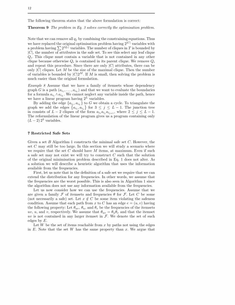
We will prove that if we have an item a coming from some inner separator andnot included in the minimal safe set, then we can alter the junction tree such thatthe item a is no longer included in the inner separators. For the sake of clarity, weillustrate an example of the modification process in Figure 4.

ab

bcx

behx deefx

gh

hix

ab

behx

bcx

efx

hix

de

gh

Fig. 4 Two equivalent junction trees. Our goal is to find the minimal safe set forB = {a, d, g}. The left junction tree is before the modification and the right is afterthe modification. We see that the attribute x is not included in the inner separatorsin the right tree. The sets appearing in the proof are as follows: The minimal safeset C is adgbeh. I consists of 3 separators bx, ex, and hx. The other separatorsbelong to J . V consists of 4 cliques bcx, efx, hix, and behx. The clique Q is behx.

Let G be the dependency graph and T the current junction tree. Let C be theminimal safe set containing B and let a /∈ C be an item coming from some innerseparator. Let us consider paths (in G) from a to its frontier. For the sake of clarity,we prove only the case where the paths from a to C are of length 1. The proof forthe general case is similar.

Let I be the collection of inner separators containing a. Let V be the collection of(inner) cliques incident to the inner separators included in I . The pair (V, I) definesa subtree of T . Let J be the set of inner separators incident to some clique in V butnot included in I . Note that each item coming from the inner separators includedin J must be included in C because otherwise we have violated the assumptionthat the paths from a to its frontier are of length 1.

The frontier of a consists of the items of the inner separators in J and of possiblysome items from the set B. By the assumption the frontier is in F and thus it isfully connected. It follows that there is a clique Q containing the frontier. If Q /∈ V ,a clique from V closest to Q also contains the frontier. Hence we can assume Q ∈ V .

Select a separator E ∈ J . Let U /∈ V be the clique incident to E. We modify thetree by cutting the edge E and reattaching U to Q. The procedure is performed toeach separator in J . The obtained tree satisfies the running intersection propertysince Q contains the items coming from each inner separators included in J . If thefrontier contained any items included in B, then Q contains these items. It is easyto see that each clique in V , except for the clique Q, becomes outer. Therefore, ais no longer included in any inner separator.

A.7 Proof of Theorem 9

Let p be the optimal distribution. Then by marginalising we can obtain pi, and qj

which produce the same solution for the reduced problem.To prove the other direction let pi, and qj be the optimal distributions for the

reduced problem. Since the running intersection property holds, we can define thejoint distribution p by p =

∏i pi/

∏j qj . It is straightforward to see that p satisfies

the frequencies. This proves the statement.