nicholas charles victor pilkingtonclassic computing problems were implemented on the gpu, and bench...
TRANSCRIPT

An Investigation into General PurposeComputation on Graphics Processing
Units (GPGPU)
Submitted in partial fulfilmentof the requirements of the degree of
Bachelor of Science (Honours)
of Rhodes University
Nicholas Charles Victor Pilkington
Grahamstown, South AfricaNovember 2007

Abstract
General Purpose Computing on Graphics Processing Units is an infant field of computerscience, and exposes exciting areas in which the power of graphics processing units canbe harnessed to solve problems that are either otherwise too computationally expensiveon conventional central processing units, or to gain increased performance. A number ofclassic computing problems were implemented on the GPU, and bench marked againstCPU implementations. Results from this testing have shown GPGPU to be viable acrossa number of different areas. An analysis model was also developed in order to give betterinsight into the expected performance of a GPGPU implementation of a problem on theoutset without having to make a comparative implementation.

Acknowledgements
The author would like to thank the Department of Computer Science at Rhodes Univer-sity, and especially his supervisor for their continued assitance and interest in this work.The author would also like to thank his mother without whose support this work wouldnot have been possible.
The author acknowledges the support of the Telkom Centre for Excellence at RhodesUniversity as well as the National Research Foundation.

Contents
1 Introduction 9
1.1 Intentions of Research . . . . . . . . . . . . . . . . . . . . . . . . . . . . . 9
1.2 Structure of Investigation . . . . . . . . . . . . . . . . . . . . . . . . . . . 9
2 Introduction to Graphics Processing 11
2.1 Evolution of Graphics Hardware . . . . . . . . . . . . . . . . . . . . . . . . 11
2.2 The Graphics Pipeline . . . . . . . . . . . . . . . . . . . . . . . . . . . . . 13
2.2.1 The Fixed Function Pipeline . . . . . . . . . . . . . . . . . . . . . . 13
2.2.2 Stages of the Graphics Pipeline . . . . . . . . . . . . . . . . . . . . 14
2.2.3 The Programmable Graphics Pipeline . . . . . . . . . . . . . . . . . 15
2.2.4 Shaders . . . . . . . . . . . . . . . . . . . . . . . . . . . . . . . . . 15
2.2.5 Different Types of Shaders . . . . . . . . . . . . . . . . . . . . . . . 16
2.2.5.1 Vertex Shaders . . . . . . . . . . . . . . . . . . . . . . . . 16
2.2.5.2 Fragment Shaders . . . . . . . . . . . . . . . . . . . . . . 16
2.2.5.3 Geometry Shaders . . . . . . . . . . . . . . . . . . . . . . 16
2.3 Summary . . . . . . . . . . . . . . . . . . . . . . . . . . . . . . . . . . . . 17
3 Introduction to General Computation on Graphics Processing Units 18
3.1 Technology Trends . . . . . . . . . . . . . . . . . . . . . . . . . . . . . . . 18
3.1.1 Computation versus Communication . . . . . . . . . . . . . . . . . 19
3.1.2 Latency versus Bandwidth . . . . . . . . . . . . . . . . . . . . . . 20
3.1.3 Smaller Power Consumption . . . . . . . . . . . . . . . . . . . . . . 20
1

CONTENTS 2
3.1.4 High-Performance Computing . . . . . . . . . . . . . . . . . . . . . 20
3.2 The GPGPU Programming Model . . . . . . . . . . . . . . . . . . . . . . . 20
3.3 Stream Programming Model . . . . . . . . . . . . . . . . . . . . . . . . . 21
3.4 Mapping Computational Concepts onto GPUs . . . . . . . . . . . . . . . . 22
3.5 GPGPU Analogies . . . . . . . . . . . . . . . . . . . . . . . . . . . . . . . 22
3.5.1 GPU Textures - Arrays . . . . . . . . . . . . . . . . . . . . . . . . 23
3.5.2 GPU Fragment and Vertex Programs – Loop Bodies . . . . . . . . 23
3.5.3 Render to Texture – Feedback Mechanism . . . . . . . . . . . . . . 23
3.5.4 Geometry Rasterization – Computation Invocation . . . . . . . . . 23
3.5.5 Texture Coordinates – Computational Domain . . . . . . . . . . . 23
3.5.6 Vertex Coordinates – Computational Range . . . . . . . . . . . . . 24
3.6 Related Work in field of GPGPU . . . . . . . . . . . . . . . . . . . . . . . 24
3.6.1 PUG . . . . . . . . . . . . . . . . . . . . . . . . . . . . . . . . . . . 24
3.6.2 Compute Unified Device Architecture (CUDA) . . . . . . . . . . . . 24
3.6.3 Close-to-Metal (CTM) . . . . . . . . . . . . . . . . . . . . . . . . . 25
3.7 Summary . . . . . . . . . . . . . . . . . . . . . . . . . . . . . . . . . . . . 25
4 Methodology 26
4.1 Performance Analysis Preliminaries . . . . . . . . . . . . . . . . . . . . . . 26
4.1.1 Speed up . . . . . . . . . . . . . . . . . . . . . . . . . . . . . . . . . 26
4.1.2 Overhead . . . . . . . . . . . . . . . . . . . . . . . . . . . . . . . . 27
4.2 Timing Considerations . . . . . . . . . . . . . . . . . . . . . . . . . . . . . 27
4.3 Testing Configuration . . . . . . . . . . . . . . . . . . . . . . . . . . . . . . 27
4.4 Language Selection . . . . . . . . . . . . . . . . . . . . . . . . . . . . . . . 28
4.4.1 Programming Language . . . . . . . . . . . . . . . . . . . . . . . . 28
4.4.2 Shader Language . . . . . . . . . . . . . . . . . . . . . . . . . . . . 29
4.4.3 Graphics API . . . . . . . . . . . . . . . . . . . . . . . . . . . . . . 29
4.4.4 Windowing API . . . . . . . . . . . . . . . . . . . . . . . . . . . . . 29
4.5 Summary . . . . . . . . . . . . . . . . . . . . . . . . . . . . . . . . . . . . 29

CONTENTS 3
5 Implementations 30
5.1 Matrix Addition . . . . . . . . . . . . . . . . . . . . . . . . . . . . . . . . . 31
5.1.1 Implementation . . . . . . . . . . . . . . . . . . . . . . . . . . . . . 31
5.1.2 Difficulties Encountered . . . . . . . . . . . . . . . . . . . . . . . . 32
5.1.3 Results . . . . . . . . . . . . . . . . . . . . . . . . . . . . . . . . . . 32
5.1.4 Performance Analysis . . . . . . . . . . . . . . . . . . . . . . . . . . 34
5.1.5 Discussion . . . . . . . . . . . . . . . . . . . . . . . . . . . . . . . . 34
5.1.6 Optimizations . . . . . . . . . . . . . . . . . . . . . . . . . . . . . . 35
5.2 Matrix Multiplication . . . . . . . . . . . . . . . . . . . . . . . . . . . . . . 36
5.2.1 Approach . . . . . . . . . . . . . . . . . . . . . . . . . . . . . . . . 36
5.2.2 Difficulties Encountered . . . . . . . . . . . . . . . . . . . . . . . . 37
5.2.3 Results . . . . . . . . . . . . . . . . . . . . . . . . . . . . . . . . . . 38
5.2.4 Performance Analysis . . . . . . . . . . . . . . . . . . . . . . . . . . 38
5.2.5 Discussion . . . . . . . . . . . . . . . . . . . . . . . . . . . . . . . . 42
5.2.6 Optimizations . . . . . . . . . . . . . . . . . . . . . . . . . . . . . . 42
5.3 Sorting . . . . . . . . . . . . . . . . . . . . . . . . . . . . . . . . . . . . . . 42
5.3.1 Methodology . . . . . . . . . . . . . . . . . . . . . . . . . . . . . . 43
5.3.2 CPU Implementations . . . . . . . . . . . . . . . . . . . . . . . . . 43
5.3.3 GPU Implementations . . . . . . . . . . . . . . . . . . . . . . . . . 44
5.3.4 Difficulties Encountered . . . . . . . . . . . . . . . . . . . . . . . . 47
5.3.5 Render to texture . . . . . . . . . . . . . . . . . . . . . . . . . . . 47
5.3.6 Coordinate Wrapping . . . . . . . . . . . . . . . . . . . . . . . . . . 48
5.3.7 Uniform Parameters . . . . . . . . . . . . . . . . . . . . . . . . . . 48
5.3.8 Results . . . . . . . . . . . . . . . . . . . . . . . . . . . . . . . . . . 48
5.3.9 Performance Analysis . . . . . . . . . . . . . . . . . . . . . . . . . . 49
5.3.10 Optimizations . . . . . . . . . . . . . . . . . . . . . . . . . . . . . . 52
5.3.10.1 Feedback Mechanism . . . . . . . . . . . . . . . . . . . . . 53
5.3.10.2 Data Encoding . . . . . . . . . . . . . . . . . . . . . . . . 53

CONTENTS 4
5.4 Searching . . . . . . . . . . . . . . . . . . . . . . . . . . . . . . . . . . . . 53
5.4.1 Approach . . . . . . . . . . . . . . . . . . . . . . . . . . . . . . . . 54
5.4.2 Difficulties Encountered . . . . . . . . . . . . . . . . . . . . . . . . 55
5.4.3 Results . . . . . . . . . . . . . . . . . . . . . . . . . . . . . . . . . . 56
5.4.4 Performance Analysis . . . . . . . . . . . . . . . . . . . . . . . . . . 56
5.4.5 Optimizations . . . . . . . . . . . . . . . . . . . . . . . . . . . . . . 58
5.5 AES Encryption . . . . . . . . . . . . . . . . . . . . . . . . . . . . . . . . . 59
5.5.1 Approach . . . . . . . . . . . . . . . . . . . . . . . . . . . . . . . . 60
5.5.1.1 Encryption Operations . . . . . . . . . . . . . . . . . . . . 60
5.5.2 Difficulties Encountered . . . . . . . . . . . . . . . . . . . . . . . . 62
5.5.3 Results . . . . . . . . . . . . . . . . . . . . . . . . . . . . . . . . . . 63
5.5.4 Performance Analysis . . . . . . . . . . . . . . . . . . . . . . . . . . 65
5.6 Rendering Fractal Images . . . . . . . . . . . . . . . . . . . . . . . . . . . 67
5.6.1 Approach . . . . . . . . . . . . . . . . . . . . . . . . . . . . . . . . 67
5.6.2 Difficulties Encountered . . . . . . . . . . . . . . . . . . . . . . . . 68
5.6.3 Results . . . . . . . . . . . . . . . . . . . . . . . . . . . . . . . . . . 68
5.6.4 Performance Analysis . . . . . . . . . . . . . . . . . . . . . . . . . . 68
5.7 Cellular Automata Simulation on a Grid . . . . . . . . . . . . . . . . . . . 69
5.7.1 Approach . . . . . . . . . . . . . . . . . . . . . . . . . . . . . . . . 70
5.7.2 Difficulties Encountered . . . . . . . . . . . . . . . . . . . . . . . . 70
5.7.2.1 Boundary Conditions . . . . . . . . . . . . . . . . . . . . . 70
5.7.3 Results . . . . . . . . . . . . . . . . . . . . . . . . . . . . . . . . . . 70
5.7.4 Performance Analysis . . . . . . . . . . . . . . . . . . . . . . . . . . 71
5.8 Summary . . . . . . . . . . . . . . . . . . . . . . . . . . . . . . . . . . . . 71
6 Discussion and Analysis 73
6.1 GPGPU Viability Analysis Model . . . . . . . . . . . . . . . . . . . . . . . 74
6.2 Future Work . . . . . . . . . . . . . . . . . . . . . . . . . . . . . . . . . . . 75

CONTENTS 5
7 Conclusion 77
Bibliography 78
A Code Listings 80
A.1 Matrix Addition . . . . . . . . . . . . . . . . . . . . . . . . . . . . . . . . . 80
A.1.1 Matrix Addition Routine . . . . . . . . . . . . . . . . . . . . . . . 80
A.2 Matrix Multiplication . . . . . . . . . . . . . . . . . . . . . . . . . . . . . . 80
A.2.1 Matrix Multiplication Routine . . . . . . . . . . . . . . . . . . . . . 80
A.3 Searching . . . . . . . . . . . . . . . . . . . . . . . . . . . . . . . . . . . . 81
A.3.1 Linear Search Routine . . . . . . . . . . . . . . . . . . . . . . . . . 81
A.3.2 Binary Search Routine . . . . . . . . . . . . . . . . . . . . . . . . . 82
A.4 Sorting . . . . . . . . . . . . . . . . . . . . . . . . . . . . . . . . . . . . . . 83
A.4.1 Odd Even Transition Sort Routine . . . . . . . . . . . . . . . . . . 83
A.4.2 Bitonic Merge Sort Routine . . . . . . . . . . . . . . . . . . . . . . 85
A.5 AES Encryption . . . . . . . . . . . . . . . . . . . . . . . . . . . . . . . . . 86
A.5.1 SubBytes Routine . . . . . . . . . . . . . . . . . . . . . . . . . . . . 86
A.5.2 ShiftLeft Routine . . . . . . . . . . . . . . . . . . . . . . . . . . . . 86
A.5.3 MixColumns Routine . . . . . . . . . . . . . . . . . . . . . . . . . . 87
A.5.4 AddRoundkey . . . . . . . . . . . . . . . . . . . . . . . . . . . . . . 88
A.6 Logical Operation Routine . . . . . . . . . . . . . . . . . . . . . . . . . . . 88
A.7 Rendering Fractal Images . . . . . . . . . . . . . . . . . . . . . . . . . . . 89
A.7.1 Mandelbrot Fractal Routine . . . . . . . . . . . . . . . . . . . . . . 89
A.8 Cellular Automata . . . . . . . . . . . . . . . . . . . . . . . . . . . . . . . 89
A.8.1 Grid Simulation Routine . . . . . . . . . . . . . . . . . . . . . . . . 89

List of Figures
2.1 The Graphics Pipeline . . . . . . . . . . . . . . . . . . . . . . . . . . . . . 13
5.1 Matrix Addition Execution Times . . . . . . . . . . . . . . . . . . . . . . . 33
5.2 Execution Time with Different Numbers of Shaders Cores . . . . . . . . . . 35
5.3 Matrix Multiplication Execution Times . . . . . . . . . . . . . . . . . . . . 39
5.4 Relative speedup of GPU Implementation . . . . . . . . . . . . . . . . . . 41
5.5 Execution Time with Different Numbers of Shader Cores . . . . . . . . . . 42
5.6 Odd Even Transition Sort . . . . . . . . . . . . . . . . . . . . . . . . . . . 46
5.7 Bitonic Merge Sort . . . . . . . . . . . . . . . . . . . . . . . . . . . . . . . 47
5.8 Render to Texture Feedback Loop . . . . . . . . . . . . . . . . . . . . . . . 48
5.9 Sorting Algorithm Execution Times . . . . . . . . . . . . . . . . . . . . . . 49
5.10 Transition Sort Asymptotic Complexity . . . . . . . . . . . . . . . . . . . . 51
5.11 Bitonic Merge Sort Asymptotic Complexity . . . . . . . . . . . . . . . . . 51
5.12 Mean Execution Time with Different Numbers of Cores . . . . . . . . . . . 52
5.13 Mean Execution Time of Searching Algorithms . . . . . . . . . . . . . . . . 57
5.14 XOR Look up Field . . . . . . . . . . . . . . . . . . . . . . . . . . . . . . . 63
5.15 AND Look up Field . . . . . . . . . . . . . . . . . . . . . . . . . . . . . . . 64
5.16 OR Look up Field . . . . . . . . . . . . . . . . . . . . . . . . . . . . . . . . 64
5.17 AES Multi-Block Encryption Rate . . . . . . . . . . . . . . . . . . . . . . 66
5.18 Mandelbrot Fractal Images . . . . . . . . . . . . . . . . . . . . . . . . . . . 69
5.19 Cellular Automata Simulation . . . . . . . . . . . . . . . . . . . . . . . . . 71
6

List of Tables
4.1 Test Platform Configuration . . . . . . . . . . . . . . . . . . . . . . . . . . 28
4.2 Graphics Cards Used . . . . . . . . . . . . . . . . . . . . . . . . . . . . . . 28
5.1 Matrix Addition Execution Times . . . . . . . . . . . . . . . . . . . . . . . 33
5.2 Execution Time with Different Numbers of Shader Cores . . . . . . . . . . 34
5.3 Matrix Multiplication Execution Times . . . . . . . . . . . . . . . . . . . . 38
5.4 Relative Speedup of GPU . . . . . . . . . . . . . . . . . . . . . . . . . . . 40
5.5 Execution Time with Different Numbers of Shader Cores . . . . . . . . . . 41
5.6 Sorting Algorithms . . . . . . . . . . . . . . . . . . . . . . . . . . . . . . . 43
5.7 Mean Execution Times of Sorting Algorithms (µs) . . . . . . . . . . . . . . 49
5.8 Relative Speedup of GPU Sorting Algorithms to Quick Sort . . . . . . . . 50
5.9 Bitonic Merge Sort with Varying Numbers of Shader Cores . . . . . . . . . 52
5.10 Searching Algorithms . . . . . . . . . . . . . . . . . . . . . . . . . . . . . . 54
5.11 Mean Search Execution Times . . . . . . . . . . . . . . . . . . . . . . . . . 56
5.12 Relative Speedup of CPU to GPU Binary Searches . . . . . . . . . . . . . 57
5.13 Mean Performance on Shader Cores . . . . . . . . . . . . . . . . . . . . . . 58
5.14 Key-Block-Round Combinations . . . . . . . . . . . . . . . . . . . . . . . . 59
5.15 AES Encryption Single Block . . . . . . . . . . . . . . . . . . . . . . . . . 63
5.16 AES Encryption Multi Block . . . . . . . . . . . . . . . . . . . . . . . . . . 63
5.17 Mean Encryption Rate . . . . . . . . . . . . . . . . . . . . . . . . . . . . . 66
5.18 Maximum Encryption Rate . . . . . . . . . . . . . . . . . . . . . . . . . . 67
5.19 Fractal Rendering Speeds . . . . . . . . . . . . . . . . . . . . . . . . . . . . 68
7

LIST OF TABLES 8
5.20 Mandelbrot Fractal Computation Rate (points/s) . . . . . . . . . . . . . . 68
5.21 John Conway Rule Set . . . . . . . . . . . . . . . . . . . . . . . . . . . . . 69
5.22 Cellular Automata Execution Time . . . . . . . . . . . . . . . . . . . . . . 70

Chapter 1
Introduction
General Purpose Computation on Graphics Processing Units (GPGPU) refers to theprocessing where by general computation is achieved on a specialized graphics processor.This type of processing opens up many new paths to computation in general. Thispaper will initially describe the intentions of this research and the evolution of graphicsprocessing hardware that have led to the inception of general processing on graphicsprocessing units [22].
1.1 Intentions of Research
The intention of this research is to gain a deeper understanding of general computationon graphics processing units in a general sense. More specifically information aboutperformance, viability and ease of implementation are sought. Ultimately information isneeded to be able to construction a test of conditions for the analysis of a problem onthe outset that will assist in deciding whether it is would be beneficial to process it on aGPU rather than a CPU. With the presentation of technology trends and developmentin hardware 2.1 it can be seen that graphics processing hardware is only going to becomemore powerful. Thus it becomes important to understand on the outset how applicablethis power is in solving certain tasks. These are the issues that this research seeks to findsolutions to.
1.2 Structure of Investigation
Section 2.2 will introduce graphics processing in general as well as graphics processingconcepts that are critical to understanding GPGPU. Section 3 will lead into a discussion
9

1.2. STRUCTURE OF INVESTIGATION 10
of the types of architecture and fundamentals which make GPGPU possible in particularthe Stream Processing Model. Section 3.6 will give a brief outline of the existing GPGPUframeworks available. Chapter 4 will give details about how the investigation was under-taken in order to resolve the intentions of the research described in 1.1. Chapter 5 willgive detailed information on how the implementations where carried out as well as presentand discuss any results obtained. A detailed discussion of these results will be providedin chapter 6 with conclusive statements given in the final chapter.

Chapter 2
Introduction to Graphics Processing
Graphics processing is the underlying foundation that supports GPGPU. It is importantto understand the technological developements that have taken place of the last 20 yearsand what impact they have had on graphics processing in general.
2.1 Evolution of Graphics Hardware
Computer hardware capabilities are advancing very fast and the discussion of this will bethoroughly dealt with in section 3.1. This section will detail the evolution of computergraphics hardware and what the major changes have been over the last 20 years as op-posed to how these changes are occurring. NVIDIA introduced the term “GPU’ in thelate 1990s to replace the archaic term “VGA controller”. The Video Graphics Controllerreleased by IBM in 1987 functioned as a frame buffer. The CPU was still fully responsiblefor updating and accessing this frame buffer. Today the CPU rarely manipulates graphicsrelated information as all this processing is done on the GPU. There have been four majorgenerations of GPU evolution. Each successive evolution has built on the previous one toproduce faster and more capable hardware. Each generation has also had influences onthe functionality of the two major 3D programming interfaces, OpenGL [7] and DirectX[4]. OpenGL is an open source standard with cross-platform functionality on Windows,Linux and Macintosh computers. DirectX is an evolving set of Microsoft multimedia pro-gramming interfaces, including Direct3D for 3D programming on Windows based systemsonly [13].
11

2.1. EVOLUTION OF GRAPHICS HARDWARE 12
Pre-GPU Graphics Acceleration
Prior to the inception of GPUs, graphics systems were developed privately by companieslike Silicon Graphics (SGI) and Evan & Sutherland [13]. These systems were far tooexpensive for personal computer users and thus did not achieve any mass market success.Normal users were limited to using their CPUs for all types of graphics processing [13].
First-Generation GPUs
The first generation of GPUs – up to 1998 – includes NVIDIA’s TNT2, ATI’s Rage, and3dfx’s Voodoo 3. These GPUs could rasterize triangles and apply one or two textures.They also implemented the DirectX 6 feature set. These graphics cards relieved the CPUof updating individual pixels. However these GPUs suffered from two major limitations.Firstly, they were not able to transform the vertices and all the transformation had tobe done by the CPU. Secondly they were relatively limited in the maths operations forcombining textures to compute the final colour of rasterizer pixels [13].
Second-Generation GPUs
The second generation of GPUs (1999-2000) included NVIDIA’s GeForce 256 and Geforce2,ATI’s Radeon 7500, and S3’s Savage3D. These GPUs can offload 3D vertex transforma-tion and lighting onto the CPU. They are also able to perform more complicated vertextransformation. Both OpenGL and DirectX 7 support hardware vertex transformation.More complicated maths operations like cube mapping were introduced making the GPUsmore configurable but still not programmable [13].
Third-Generation GPUs
The third generation of GPUs (2001) includes NVIDIA’s GeForce 3 and GeForce 4 Ti, Mi-crosoft’s Xbox, and ATI’s Radeon 8500. This generation offered programmability insteadof just more configurability. It let the application specify the sequence of instructions forprocessing vertices instead of using pre-programmed transformation and lighting func-tionality. The pixel operations were also more configurable but not truly programmable,as the generation was transitional [13].

2.2. THE GRAPHICS PIPELINE 13
Figure 2.1: The Graphics Pipeline
V e r t e x T r a n s f o r m a t i o nP r i m i t i v e A s s m b l y a n d R a s t e r a t i o n
F r a g m e n t T e x t u r i n g a n d C o l o u r i n g
R a s t e r O p e r a t i o n s
Fourth-Generation GPUs
The fourth generation of GPUs (2001 – 2006) included NVIDIA’s GeForce FX family,ATI’s Radeon 9700. These GPUs boasted fully programmable vertex as well as pixelshaders. DirectX 9 and OpenGL both exposed the programmability of these shaders [13].
Fifth-Generation GPUs
The fifth generation of GPUs are only just emerging now in 2007 and include NVIDIA’sGeForce 8 family and ATI’s Radeon R600. The ATI Radeon R600 is still to be releasedand as such details are scarce. NVIDIA’s GeForce 8 includes a unified shader model wherevertex and pixel shaders execute on generic shader cores instead of specialized ones [13].
2.2 The Graphics Pipeline
The graphics pipeline is the central core of graphics processing. It can be thought of as asequence of stages operating in parallel in a fixed order. Each stage of the pipeline receivesinformation from the previous stage, performs some operation on it and then passes it onto the next stage in the pipeline. The graphics pipeline in analogous to an assembly linein a factory, where each stages builds upon the previous one. It is important to have agood grasp of what each stage receives and produces as well as a detailed understandingof what operations are performed and in what order they occur.
2.2.1 The Fixed Function Pipeline
The fixed function pipeline was limited in what could be performed at each stage. Thiswas not initially a problem as the performance gained from some graphics processingbeing offloaded from the CPU was enough to justify the process. Figure 2.1 presents asimple graphics pipeline architecture.

2.2. THE GRAPHICS PIPELINE 14
2.2.2 Stages of the Graphics Pipeline
The graphics pipeline is broken up into various stages that each perform a specific purpose.
Vertex Transformation
This is the first stage of the pipeline and receives a list of vertices. Vertex transformationperforms various mathematical operations on each vertex. Examples of this are changingthe colour associated with a vertex, changing its position or altering texture coordinatesets. Many operations are possible especially due to the programmable nature of thevertex shader which allows programmers to write their own programs that execute inthe vertex transformation stage. The transformed vertices are passed on to the primitiveassembly and rasterization stage [13, 14].
Primitive Assembly and Rasterization
This stage of the pipeline receives a list of transformed vertices and is responsible forassembling them into their composing primitives. Batches of vertices paired with theirgeometric batching information are assembled into primitives like triangles and quads.Some of these primitives may be clipped to the view frustum. This process is calledculling. The surviving polygons are rasterized. This is the process whereby each primitiveis deconstructed into the set of pixels and fragments. Pixels correspond to the contentsof a frame buffer element where as fragments are the information necessary to generatean actual pixel. The resulting fragments are passed onto the fragments texturing andcolouring stage [13, 14].
Fragment Texturing and Colouring
The fragments passed into this stage are interpolated and various mathematical operationsare executed on the interpolated values. This stage of the pipeline is concerned withdetermining the final colour of the pixel that should be written to the frame buffer.The fragment may be discarded at this stage based on specified criteria like depth. Theresulting fragments, if any, are passed to the raster operations stage [13, 14].
Raster Operations
This stage performs various operations on the fragment received to determine whether ornot it should be discarded. These operations can include hidden surface removal, scissor

2.2. THE GRAPHICS PIPELINE 15
tests, depth tests and alpha tests. The fragment may need to be combined with thecurrent pixel in the frame buffer. This operation is called blending. This stage finallyupdates the frame buffer with the correct value [13, 14].
2.2.3 The Programmable Graphics Pipeline
With the advent of the fourth generation of GPUs discussed in sub-section 2.1, stagesof the graphics pipeline have become fully programmable. These stages are the VertexTransformations stage and the Fragment Texturing and Colouring stage as depicted infigure 2.1. Programs known as shaders can be written which are executed at these stagesof the pipeline and control the operations performed. Herein lies the power of GPGPU asa previously inaccessible piece of hardware in the fixed function graphics pipeline is nowprogrammable [9, 16, 13].
2.2.4 Shaders
Prior to the inception of GPUs, CPUs did all the graphics processing required by aprogram. GPUs are a specialized type of CPU that is capable of performing graphicsspecific computations much faster than a CPU can. The first of these GPUs were highlyspecialized and there was no way to program the graphics pipeline. As advances weremade in the field of computer graphics there was more of a need to make the pipelinebecame more programmable. The need for the development of a language to programgraphics hardware was evident and the spawned three different shader languages GLSL[6], HLSL [3]and Cg [13, 9].
OpenGL Shading Language (GLSL)
GLSL is an acronym for OpenGL Shading Language and is also known as GLslang. GLSLis a high level shading language based on the C programming language. It was createdby the OpenGL Architecture Review Board to give developers more direct control of thegraphics pipeline without having to use assembly language or hardware-specific languages.GLSL has cross platform compatibility on multiple operating systems, including Macin-tosh, Windows and Linux. GLSL also has the ability to write shaders that can be usedon any hardware vendor’s graphics card that supports the OpenGL Shading Language.Each hardware vendor includes the GLSL compiler in their OpenGL driver, thus allow-ing each vendor to create code optimized for their particular graphics card’s architecture[13, 27, 6].

2.2. THE GRAPHICS PIPELINE 16
High Level Shading Language (HLSL)
The High Level Shader Language or High Level Shading Language (HLSL) is a proprietaryshading language developed by Microsoft for use with the Microsoft Direct3D API. It isin competition with GLSL shading language, but is not compatible with the OpenGLstandard. It is very similar to the NVIDIA Cg shading language [9, 3].
C for Graphics (Cg)
Cg or C for Graphics is a high-level shading language created by NVIDIA for programmingvertex and pixel shaders. Cg is based on the C programming language and although theyshare the same syntax, some features of C were modified and new data types were addedto make Cg more suitable for programming graphics processing units [13].
2.2.5 Different Types of Shaders
There are three different types of shaders each with a different specific purpose and formof operation.
2.2.5.1 Vertex Shaders
Vertex shaders Vertex shaders operate on vertices in the stream. They can be usedto change and manipulate information like texture coordinates and positions or otherattributes associated with a vertex.
2.2.5.2 Fragment Shaders
Fragment shaders are also called pixel shaders. They operate on pixels in the stream andcan be used to change and manipulate information like colour and lighting values. Theytake fragments as their input fragments and then perform various operations and outputthe augmented fragment.
2.2.5.3 Geometry Shaders
Geometry shaders are a new type of shader that allows vertices to be created and de-stroyed. This allows for generation of geometry in the pipeline which is something thatwas previously impossible with just vertex and fragment shaders. Geometry shaders wereonly supported in hardware with the advent of DirectX 10.

2.3. SUMMARY 17
2.3 Summary
Graphics processing has evolved vastly over the past twenty year and these advanced-ments, among other features, have allowed for more programmabiliy. The fixed functiongraphics pipeline has been replaced by the more robust progammable graphics pipeline.This is the foundation for general computation on graphics hardware. Programminggraphics hardware would not be possible unless hardware developers exposed this to pro-grammers. The advent of shaders technology paired with the programmable pipelineallows programmers to write fragment and pixel shaders that execute on the GPU anduse its resources.

Chapter 3
Introduction to General Computationon Graphics Processing Units
As discussed in the introduction, general-purpose computing on graphics processing units(GPGPU) refers to programming where operations are performed on the GPU ratherthan on the CPU. The advantage of such processing is that the GPU is able to performoperations in parallel where as a single core CPU cannot. Since the GPU is able to processin parallel, problems of a parallel or streaming nature could benefit from being processedon the GPU. This processing offload has previously not been possible because of thelimited accessibility of the fixed function graphics pipeline discussed in sub-section 2.2.1.The advent of programmable graphics pipelines (sub-section 2.2.3) allows non-graphicsrelated processing to take place on the GPU. This is done by means of the shaders.Instead of processing graphics information specific for rendering we may choose to havethe information we are processing represent something different. This interpretation ofdata is still transparent to the GPU as it processes the data in the same way that it wouldgraphical information [17, 15].
3.1 Technology Trends
This section will describe the evolution of CPU power and give insight into the way GPUprocessing power and functionality will tend towards in the future. Every year the powerof conventional CPUs increases and advances in the underlying technologies allow formore processing power to be crammed onto the chip. Each successive generation of CPUsis faster, has more processing power and is sometimes even cheaper. A lot can be gainedby considering the trends in this development. Processors are constructed from millions
18

3.1. TECHNOLOGY TRENDS 19
of electronic switching devices called transistors and the number of these transistors ona processor is quite an accurate metric for its processing power. In 1965, Gordon Moorepredicted that the power of CPUs would continually double each year. This prediction isknown as Moore’s Law [5]. Each new generation of CPUs increase the number of thesetransistors and also decreases their individual size. Smaller transistors can operate fasterthan larger ones as they require less current. This increase in transistor speed resultsin an increased clock speed, which is the speed of the global chip clock which is used tosynchronize processor operation. This exponential increase in computing power looks tocontinue at the current pace for at least another decade.
Semiconductor computer memory also benefits from these technology advances. TheITRS predicts than Dynamic Random Access Memory (DRAM) will continue to doublein capacity every three years. The metric for measuring DRAM is not the same as thatof CPUs. Instead they are measured in terms of bandwidth, which is the total amount ofdata they can transfer each second, or latency which is the amount of time that elapsesbetween data being requested and returned. Though both latency and bandwidth continueto increase annually they are by no means increasing at the same rate as CPU speeds[17, 10, 8, 13].
Overall the trends of both processor and memory speed and capabilities are scheduled tocontinue to increase in the coming years. We have seen that there are two separate metricfor comparing both CPUs and DRAM. For CPUs they can be graded by this clock speed,a factor that is driven by decreasing the size of the individual transistor. CPUs can alsobe graded by transistor count which is the number of transistors on the actual chip, wheremore transistors yield more advanced processing capabilities. However with an increasednumber of transistors comes increased chip size. The most important consequence ofthese technology trends is the difference between them. When one of the metric increasesfaster than the other it starts to create a specialization shift. The following section willdescribe how this gap will help drive the GPU architecture of the future. There are threemajor issues to consider in this regard: computation versus communication, latency versusbandwidth, and power [17, 10, 8, 13].
3.1.1 Computation versus Communication
As chips’ physical size increases as manufacturers put more and more transistors on them,the amount of time required for the electrical signal to travel across the chip increases.This amount of time is measured in clock cycles in current processors. Moore’s Lawcan characterize the trend in the amount of transistors growing faster than the rate at

3.2. THE GPGPU PROGRAMMING MODEL 20
which their size is decreasing as an increase in communication when compared to cost ofcomputation [17, 10, 8].
3.1.2 Latency versus Bandwidth
The gap between memory bandwidth and latency is another factor that could drive thearchitectural trend in GPUs. Latency will improve more slowly than bandwidth designersshould seek to implement solutions that are able to do more processing while the data iswaiting to be returned [17, 10, 8].
3.1.3 Smaller Power Consumption
Smaller transistors require less power; however the number of transistors being placedonto chips in increasing faster than the amount at which the power per transistor isdecreasing. This leads to each successive generation of processor needing more power tooperate [17, 10, 8].
3.1.4 High-Performance Computing
Simply providing large amount of computation is not sufficient. Efficient management ofcommunication is necessary to feed the computation resources on the chip [17, 10, 8].
Building a high performance processor requires that the computation as well as the com-munication are efficient. The reason why CPUs perform poorly in high performance ap-plications is their serial programming model. The von Neumann architecture is inherentlysequential, and does not expose parallelism and communication patterns in application.There is an alternative way of structuring programs that allows for very high efficiencyin both computation and communication. This programming model is the basis for pro-gramming GPUs today and is known as the Stream Programming Model [10].
3.2 The GPGPU Programming Model
Programming for GPUs is not like programming a different type of CPU. The biggestdifference is that a GPU is not a serial processor like a CPU. CPUs are based on thevon Neumann architecture. Simply speaking this means that they implement a Universal

3.3. STREAM PROGRAMMING MODEL 21
Turing Machine and operate in a purely sequential way, executing instructions in a serialnature and updating program memory as they go [18].
A GPU is a stream processor and instead executes on elements of an input stream andprocessing the corresponding elements of the output stream. The stream programmingmodel will be discussed in more detail in 3.3. The important difference here is that thefunction is invariant of the element of the input stream and is not dependent on anyof the other elements. Thus the order of this function executing is not important andthere are no dependencies between elements. This permits the entire input stream to beprocessed in parallel. Another way to think about this model of execution is that it is theapplication of a function to an array of data [22, 26, 10, 19, 29].
3.3 Stream Programming Model
In the stream processing model all data is represented as a stream. These streams can bethought of as an ordered set of data of the same type. The type of data in the stream canbe very simple (a stream of integers or floating-point number) or it could be more complex(a stream of points or matrices). These streams can be of any length however efficiencyis higher on longer streams with uniform data. There are a number of functions thatcan be executed on streams and they include; copying them, deriving sub-streams fromthem, indexing into them with a spate index stream and finally performing computationon them with kernels .
Kernels operate on an input stream and produce a corresponding stream of output el-ements. The defining characteristic of kernel is that they do not operate on individualelements. Kernels can be thought of as the evaluation of a function on each elementof an input stream. This is in many ways similar to the ‘map’ operation of functionalprogramming. The kernel could perform one of several operations like expansion, wheremore than one element is produced from a single input, reductions, where more than oneinput element is combined into a single output element, or filters, where only a subset ofinput elements are output[17, 10, 8, 13].
Computation on a single stream element does not depend on any of the other elementsof the stream and as a result is purely a function of the input element. This restrictionis very favorable as it means that the input stream type is completely known at the timeof compilation and can be optimized as such, but even more favorable is the fact thatthis independence implies that the order of computation of the mapping is unimportantwhich ultimately means that what appears to be a serial kernel operation can actually be

3.4. MAPPING COMPUTATIONAL CONCEPTS ONTO GPUS 22
executed in parallel [17, 10, 8, 13].
While applications can be constructed by chaining together the inputs and output ofvarious streams, whereby the output of one stream becomes the input of the next one,the graphics pipeline is traditionally structured as stages each depending on the resultof the immediate previous stage. This makes the graphics pipeline a good match for thestream programming model as it is analogous to the stream and kernel abstraction justdescribed [17, 10, 8, 13].
3.4 Mapping Computational Concepts onto GPUs
The previous sections have described the stream programming model in detail howeverit is still necessary to have a good understanding of what types of computations aremore effectively performed on a GPU using the stream programming model and howthese computations can be mapped to GPU programming. In order to attain maximumperformance a highly detailed understanding of the underlying architecture is required.This is also true with traditional CPU programming. The previous sections have providedan understanding of the stream programming model as well as the graphics pipelineand shaders. They have also provided information pertaining to the types of trendsthat will drive development in this area in the future. This information is necessary inunderstanding how concepts are mapped to GPUs. The design of a GPU is very importantto keep in mind when programming one. This is the same with CPUs although becauseof their more generic nature it is possibly not as important unless you are seeking highlyspecialized fast computation. We know that a GPU exploits high data parallelism andindependence in the graphics pipeline in order to gain performance [23, 17].
3.5 GPGPU Analogies
Even knowing what resources are available on the GPU and what they can do, it canstill be difficult for someone not well versed in graphics programming to understand howthe GPU can be used for ordinary programming. This section will present a number ofmetaphors that will allow for a better grasp of the possibilities and concepts of GPGPUand how they can be mapped to the stream processing model and in turn the graphicspipeline [23, 17].

3.5. GPGPU ANALOGIES 23
3.5.1 GPU Textures - Arrays
GPUs have no concept of primitive arrays. However they do support textures and vertexarrays. These are the natural choice for the representation of array based data. Anyinformation that we would ordinarily store in an array can be stored in texture. The waythat the information is stored is up to the programmer [23, 17].
3.5.2 GPU Fragment and Vertex Programs – Loop Bodies
The shader programs operate on each element of the input stream. They can be thought ofas a loop over the stream and executing a kernel program on each element. For this reasonshaders can be thought of as the loop bodies in terms of conventional CPU programming,where the loop is over the elements of the stream [23, 17].
3.5.3 Render to Texture – Feedback Mechanism
As mentioned earlier the render to texture mechanism can be used to pass the outputof on iteration into the input of the next. For this reason it can be used as a feedbackmechanism – something that is trivial to implement on a CPU because of the unifiedmemory model of the von Neumann architecture. Render to texture can be used to writethe output of a fragment program to memory and use it in the next execution of thefragment program. This concept will be describe more fully when used later on [23, 17].
3.5.4 Geometry Rasterization – Computation Invocation
It is all very well to have methods in place for memory, processing and feedback but thereneeds to be a mechanism to control the overall execution. In other words there needs tobe a start condition that will initialize execution. This is achieved by some initial inputstream data. This is actually very simple as it just means generating some geometry. InGPGPU processing is generally on every element of a rectangular stream representing agrid. Therefore the most common invocation is to simply render a quadrilateral [23, 17].
3.5.5 Texture Coordinates – Computational Domain
The range of the computation is based on the texture coordinates associated with thevertices of the primitive. The rasterizer linearly interpolates between the texture coordi-

3.6. RELATED WORK IN FIELD OF GPGPU 24
nates specified, four in the case of a quadrilateral, in order to generate the coordinatesfor each fragment which are then passed to the fragment program [23, 17].
3.5.6 Vertex Coordinates – Computational Range
As discussed before the computational domain is generated depending on which verticesare passed into the pipeline. These vertices are the values interpolated between to generatethe texture coordinate input (domain) of the fragment program. Therefore the initiallygenerated vertices dictate the range of the resulting outputs of the fragment shader [23, 17].
3.6 Related Work in field of GPGPU
This section will briefly present two different frameworks for computation on the GPU.
3.6.1 PUG
Is a simplistic framework for GPGPU written in C++ and is effectively an abstractionof the OpenGL calls necessary to facilitate the execution of a program on the GPU. Isdoes not provide any abstraction for the programming of the actual vertex and fragmentshaders. It implements general reductions and provides abstractions for domain and rangebinding as well as the render to texture mechanism outlined in sub-section 3.5.3 [10, 17].
3.6.2 Compute Unified Device Architecture (CUDA)
CUDA is an acronym for Compute Unified Device Architecture. The CUDA Toolkit isa complete software development solution for programming CUDA-enabled GPUs. Itprovides build in functionality for complex operations like Fast Fourier Transforms andvarious numerical algorithms. CUDA uses C to create the kernel programs that areotherwise written in some shader language. CUDA also facilitates direct implementationof parallel computations in the C language using an API designed for general-purposecomputation instead of having to write transformed code in a graphics API like OpenGLor DirectX [10, 17].

3.7. SUMMARY 25
3.6.3 Close-to-Metal (CTM)
CTM is an acronym for Close-to-Metal which is a hardware interface developed by ATIto allow programmers to interface directly with the hardware. It exposes access to theinstruction set and operations of the GPU and facilitates GPGPU [1].
3.7 Summary
The trend in processor speeds is still exponential growth however, GPU and CPU memorytrends differ. CPU memory speeds are increasing very slowly but the density is stillincreasing fast. Graphics card memory density is increasing but so is the bandwidth.This allows for a very width bandwidth channel for communication between the GPU andvideo memory. this massive bandwidth is not available on standard processing platformand is an important characteristic that can facilitate very high performance on the GPU.GPGPU is a difficult concept to understand as the problem needs to be formulated ina graphics related way. The analogies provided assist in this regard making it easier tothink of a problem in terms of graphics processing capabilities. Finally NVIDIA and ATIboth have framework and interfaces available for direct GPGPU on their cards. Theseframeworks, namely CUDA and CTM expose programmability of the graphics hardwareto programmers allowing for general purpose computation.

Chapter 4
Methodology
On the outset, it was sought to investigate GPGPU in a general sense. In order to dothis, a comparison needs to be drawn between GPU and some thoroughly understoodtechnology. The logical choice to compare GPU processing to would be conventionalprocessing on a CPU. For this reason in order to investigate GPGPU thoroughly a numberof test programs were created to be executed on the GPU. These programs are each veryspecific in themselves but together cover a broad area of different problem domains. Foreach program developed for the GPU, a CPU control version was developed to give acomparison. This gives a solid foundation from which to launch more detailed statisticalanalysis of the GPU and CPU implementations and be able to draw accurate conclusionsabout performance and viability.
4.1 Performance Analysis Preliminaries
As detailed in the 3.2, a GPU is inherently a parallel processor. The analysis of parallelprocessing performance differs from that of sequential processing and it is important tounderstand the ways in which performance can not only be measured, but also compared.
4.1.1 Speed up
Speed up refers to how much faster one algorithm is than another one. This will be auseful metric to use in the comparison of an GPGPU algorithm and a standard CPU one.Speed up is defined by the following formula:
S =T1
T2
26

4.2. TIMING CONSIDERATIONS 27
where:
S is the speed up factor
T1is the execution time of the slower algorithm
T2is the execution time of the faster algorithm
4.1.2 Overhead
Overhead is the term given to parts of a program that are not directly related to the corealgorithm to be executed. Overhead may include code to initialize data or free memoryafter use.
4.2 Timing Considerations
In order to gain a better understanding GPGPU performance and to seek solutions tothe research intentions in sub-section 1.1, a high resolution (microsecond) timer was nec-essary to time fragments of code in order to generate the data for statistical analysis. Intiming code there are a number of factors that can either be included or excluded andconsideration is required in order to set a uniform way which to time the code and thusgain the most accurate results possible. A micro-second timer was used in the code totime the execution length of the addition process. For this exact purpose the followingwere adhered to in timing all code.
The initialization of the matrices and timing mechanisms were not timed as these con-tribute to overhead (see sub-section 4.1.2) rather than the actual algorithm being exe-cuted. Where time was not the standard performance metric, for example in the datarelated implementations, data throughput was measured instead.
4.3 Testing Configuration
In timing the implementations each different implementation was run on each differentsized data set 500 times. The average of these run times was then used as the time for thatspecific implementation and data set size. This average was computed as the standardarithmetic mean. More formally if xi are timing results for a specific implementation anddata set size, then the average time x is computed as:

4.4. LANGUAGE SELECTION 28
Table 4.1: Test Platform Configuration
Category DetailsProcessor Intel Core 2 Duo (1.86Ghz)Memory 2048MB DDR2 (400Mhz)Graphics NVIDIA GeForce 7900 GT (256MB), Driver Version: 91.47
Mainboard Intel Corporation Q965Hard drive 80GB SATA
Operating System Windows XP Service Pack 2
Table 4.2: Graphics Cards UsedGraphics Card Shader Cores
NVIDIA Geforce 5200 FX 4NVIDIA Geforce 6600 LE 8NVIDIA Geforce 7900 GT 24
x̄ = 1500
· ∑500i=1 xi
All runs were executed on the machine specification detailed in table 4.1. All statisticgraphs were produced using the statistical language R [28].
Where shader core performance was investigated within some implementations the fol-lowing graphics cards listed in table 4.2 were used.
4.4 Language Selection
There is a lot of choice available for selecting APIs and language for implementingGPGPU.
4.4.1 Programming Language
C++ was used as the programming language for the implementations. C++ is the defacto in graphics applications and is well established and powerful enough to support thefeatures required.

4.5. SUMMARY 29
4.4.2 Shader Language
Cg was selected as the shading language of choice. The reasn for this is that Cg is notaligned with a specific graphics API like HLSL and GLSlang.
4.4.3 Graphics API
The OpenGL API was used for the graphics processing. OpenGL was chosen over DirectXfor simplicity. The work done was not an excercise primarily in graphics processing anda simple API was needed for geometry generation and shader bindings but little else wasrequired of it.
4.4.4 Windowing API
The Windows API was used for all windowing. The reason for this is that the GLUTlibrary supports Windows effectively and makes the generation of windows and OpenGLgraphics context simple.
4.5 Summary
The methodology is intended to facilitate performance analysis of GPGPU. Choices ofprogramming language, shader language, windowing API and graphics API were all keptconstant throughout to ensure accurate statistical results. The information generatedfrom this testing methodology formed the basis of the investigation.

Chapter 5
Implementations
This chapter provides detailed information on the program suite implemented to perfor-mance test the GPU. The programs were selected to cover a broad range of computationaltasks including, floating point processing, searching, sorting as well as data intensive op-erations. Each section is presented with information about how the implementation wasperformed on both the CPU and GPU as well as detailed results and performance analysis.Source code listings of fragments of all the GPU programs are given in Appendix A andspecific references to them are given in each implementation’s section. The programs wereimplemented with simplicity in mind, this means that no specific optimizations or earlyouts for special cases were accommodated for. The reason for this was the descriptionof the research intents in section 1.1. A general investigation into GPGPU was soughtand as a result canonical implementations provided the most accurate numerical datathat was then used to gain better insight into performance in general. This simplificationmade the programs more general both from a software and a hardware point of view.Where assumptions and simplification have been made they have also been described andmotivated in detail with reasons. The remainder of the chapter is dedicated to the actualimplementations as just described.
Seven different problem domains were tackled namely: matrix addition, matrix multipli-cation, sorting, searching, AES encryption, rendering fractal images and finally cellularautomata simulations. A section is dedicated to each of the implementations and givesinformation about the implementation, results, optimizations and performance analysis.All code is also in the accompanying CD.
30

5.1. MATRIX ADDITION 31
Algorithm 1 Matrix Addition
def matrixAdd(int A[][], int B[][], int C[][])for i := 1 to n dofor j := 1 to n doC[i][j] = A[i][j] + B[i][j]
endend
end
5.1 Matrix Addition
Adding matrices is a common operation in linear algebra and forms the foundation formore complex mathematical operations in linear algebra. Addition of two matrices isachieved by summing the matrices on a per element basis. For example: 1 2
3 4
+
2 4
6 8
=
3 6
9 12
For this reason only matrices of the same size may be added together. This implementationwill only be dealing will matrices which are both, square and have a dimension thatis a power of two. The reasons for these choices is discussed further in section 5.2.2.Sequentially this operation takes n2 operations where n is the dimension of the matrix.
5.1.1 Implementation
The source code for the GPU implementation of matrix addition can be found in AppendixA.1.1. What follows is a brief discussion of how the solution was implemented on boththe CPU and the GPU.
CPU Implementation
The CPU matrix addition program initialized two square matrices of dimension 32, 64,128, 256, 512 and 1024 and added them together. The elements of the matrix wererandomly generated integers in the range [0..255]. This was done using a simple nestedloop. The matrices were represented and stored in two dimensional arrays.
GPU Implementation
The matrix addition program was implemented for the GPU using a single fragmentshader. Two square textures where first created. The red channels of the texture elements
5.1. MATRIX ADDITION 32
were then initialized to the values of the matrices that were to be added together. Thesewere random numbers in the range [0..255]. A fragment shader was then created whichsimply made a texture look up to each of the two texture units and set the red channel ofthe current pixel to the sum of the red channels in the two textures. In order to performthe actual addition operation there needed to be geometry on which the fragment shadercould operate. This was achieved by rendering a screen sized quad with the two texturesbound to it.
5.1.2 Difficulties Encountered
A number of issues come to the surface even from implementing such seeming simpleprograms on the GPU. These difficulties serve an important purpose as they add insightinto the holistic investigation of general computation on graphics processing units.
Non-power of two matrices
Earlier it was stated without reason that the problem domain would be limited to powerof two sized square matrices only. The reason for has to do with graphics processing ingeneral. Textures are much more easily dealt with when they are powers of two, andexpose various speed and space optimizations that graphics cards can take advantageof to squeeze the maximum amount of performance out of the hardware. Although thisrestriction has been relaxed in modern graphics processing and most hard can easily handlenon-power of two texture sizes it is sometimes done through various non standardizedextensions. Since it was initially stated in sub-section 5.5.1.1 that implementation weremade to be be canonical and general wherever possible. It is for this reason that textureswere constrained to be powers of two only.
5.1.3 Results
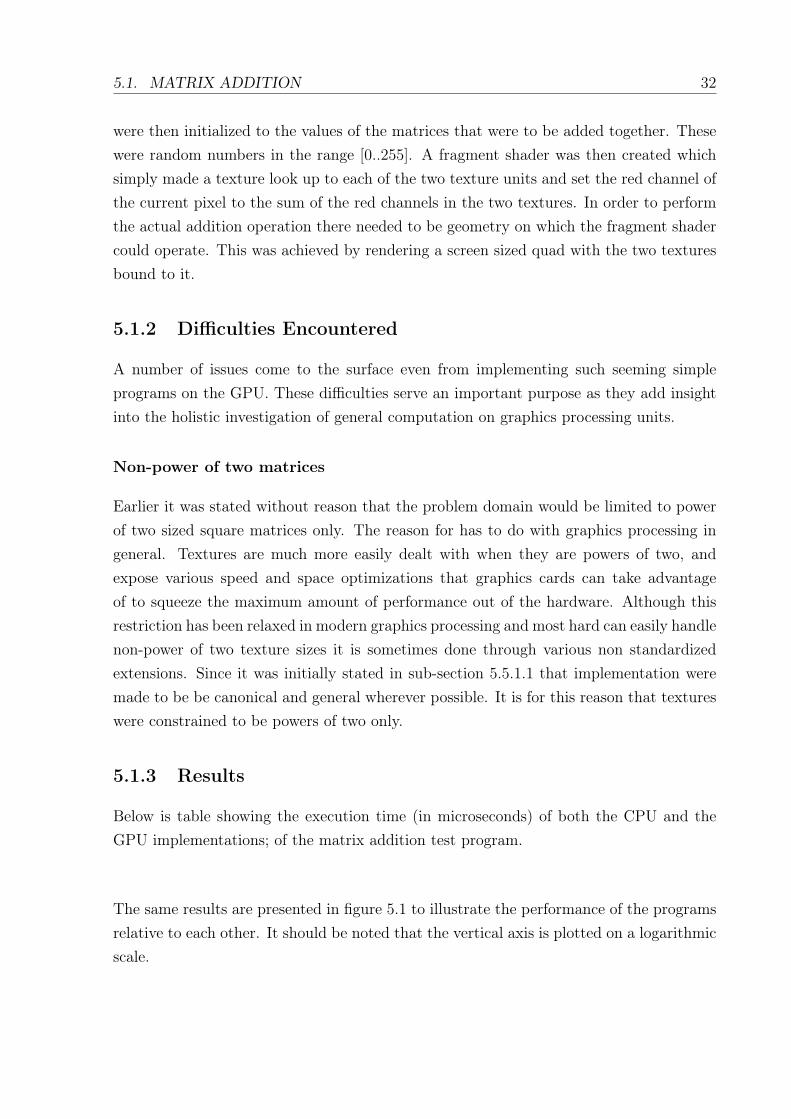
Below is table showing the execution time (in microseconds) of both the CPU and theGPU implementations; of the matrix addition test program.
The same results are presented in figure 5.1 to illustrate the performance of the programsrelative to each other. It should be noted that the vertical axis is plotted on a logarithmicscale.

5.1. MATRIX ADDITION 33
Table 5.1: Matrix Addition Execution TimesSize CPU (µs) GPU (µs) Relative Speedup on GPU32 15,265.47 6,571.05 2.3264 62,533.16 6,476.21 9.66128 228,699.98 7,867.24 29.07256 866,427.22 6,720.12 128.93512 3,430,212.74 6,698.01 512.121024 13,551,552.88 6,722.94 2,015.72
Figure 5.1: Matrix Addition Execution Times
32x32 64x64 128x128 256x256 512x512 1024x1024
Data set size
Log
Mea
n E
xecu
tion
Tim
e (m
icro
seco
nds)
05
1015
CPU Matrix AdditionGPU Matrix AdditionCPU Matrix AdditionGPU Matrix Addition

5.1. MATRIX ADDITION 34
Table 5.2: Execution Time with Different Numbers of Shader CoresNumber of Shader Cores Mean Execution Time (µs)
4 7,851.548 6,711.0624 5,225.04
5.1.4 Performance Analysis
The quadratic growth of the sequential matrix addition on the CPU can clearly been seenfrom the execution time. This is behavior that is expected as when the input size doubles,the numbers of elements in the matrix increases by a factor of four. Since the algorithmis being executed sequentially on a single core this inherently decreases the speed of thealgorithm executing by a factor of four. The execution times of the GPU version exhibitsvery different behavior. The time to add two matrix appears totally independent of thedata size and varies very little with the input size. Even large matrices were addedseamlessly with speed differences of the various data size differencing by no more that a500th of a second. The mean execution time of the GPU program across all input sizeswas: µGPU = 6, 843 where as the mean execution time of the CPU version across all inputsizes is µCPU = 3, 025, 782. The relative speedup of the GPU implementation to the CPUimplementation is therefore:
S = µCPU
µGPU= 442.17
This shows that the GPU implementation executed approximately 442 times faster thanthe CPU across all input sizes or in other words exhibited a speed increase of 44, 200%.
5.1.5 Discussion
The GPU implementation shows impressive speedups and it is important to understandwhy this is the case. As discussed in section 5.5.1.1 the matrix addition is self containedwithin a single shader. This means that the results of the addition operation is computedin a single pass and there is not need for a feedback mechanism. Another factor to consideris that the operation of matrix addition is very parallelizable. Since the result of eachcells computation is independent of all other that can be performed on separate cores. Itwould be logical to assume that the number of shaders cores on the graphics would havean impact on the performance.

5.1. MATRIX ADDITION 35
Figure 5.2: Execution Time with Different Numbers of Shaders Cores
4 8 24
Number of Shader Cores
Mea
n E
xecu
tion
Tim
e (m
icro
seco
nds)
020
0040
0060
00
It can be seen from figure 5.2 that this is indeed the case and as the number of shadercores on the graphics card is increased, so the load density across the cores decreases andthe therefore so does the execution time.
5.1.6 Optimizations
Although the GPU implementation is considerably faster than the CPU one there is roomfor improvement. As mentioned in 5.5.1.1 the elements of the matrix were only encodedinto the red channel of the texture. This left the green, blue and alpha channels unused.A better approach to the problem, which could yield even better results, would be to usea single texture and store the two matrices in its red and green channel then computethe sum and write it to the blue channel. This would require only a single texture lookup compared to two texture look ups in the previous methods. Similarly since onlyone texture is being used the amount of memory required would be halved. Using thissame principle four matrices could be encoded in a single texture allowing for even moreadditions to be performed with little extra overhead.

5.2. MATRIX MULTIPLICATION 36
5.2 Matrix Multiplication
Given the large speed up of matrix addition on the GPU that was discovered in section5.2.4 a logical progression was to attempt a more complicated and expensive operationin linear algebra. Matrix multiplication is a very computationally intensive operation. Inorder to multiply two matrices together we require first that the number of columns of thefirst matrix is equal to the number of columns in the second. It is assumed that we willbe dealing with square matrices of the same size for the same reasons as were discussedin section 5.1.2. Multiplication of two matrices results in a third matrix which has thesame number of rows as the first matrix and the same number of columns as the second.In order to multiply two matrices together the elements of each row of the first matrixare pairwise multiplied with the elements of each column in the second matrix and addedtogether in place. More formally if A is an m-by-n matrix and B is an n-by-p matrix, thentheir product is an m-by-p matrix denoted by AB (or sometimes A · B). The product isgiven by
(AB)ij =∑n
r=1 airbrj = ai1b1j + ai2b2j + · · · + ainbnj.
For example: 1 2
3 4
.
2 4
6 8
=
21 30
45 64
A sequential implementation of three nested loops to perform the operation would havea complexity of O(n3) where n is the dimension of the matrices being multiplied. Thisvalue was one of 32, 64, 128, 256, 512 or 1024. It can be seen that this may becomeinfeasible to attempt to run a sequential algorithm of this order for even relatively smallvalues of n.
5.2.1 Approach
The source code for both the CPU and GPU implementation is listed in Appendix A.2.1.The problem of matrix multiplication is not as easily implemented on the GPU as matrixaddition and the following section details exactly how it was achieved.
CPU Implementation
The CPU implementation of a matrix multiplication is simple and can achieved usingthree nested loops. The pseudo code to achieve this is listed in algorithm 2.

5.2. MATRIX MULTIPLICATION 37
Algorithm 2 Matrix Multiplication
def matrixMultiply(int A[][], int B[][], int C[][])for i := 1 to n dofor j := 1 to n dofor k := 1 to n doC[i][j] = C[i][j] + A[i][k]*B[k][j];
endend
endend
GPU Implementation
The matrix multiplication program was implemented for the GPU using a single fragmentshader in a similar fashion to the matrix addition. The red colour channels of two textureswere used to store the values of the two matrices to be multiplied. A fragment shaderwas then created which represented the operation to be performed on each element of theproduct matrix C. The function of the shader is then to compute the final value of theresulting element in a single pass. This now introduces an interesting problem of havingto read information from another element in the matrix. The solution to this problemwill be discussed further in section 5.2.2. The simplest approach is to reformulate matrixaddition as a series of dot product computations. An arbitrary element in the productmatrix C, say cij is the dot product of the row i of A and the column j of B. The resultingvalues is then outputted into the red channel of the render target.
5.2.2 Difficulties Encountered
Implementing Gather
As mentioned earlier matrix multiplication showed the need to read from resources notbound to the fragment shader. When the fragment shader was called is had two texturecoordinates bound to it, one corresponding to the matrix A and the other to matrix B.The problem is that this is not enough information to compute the total value of thecurrent matrix element. This is a technique called gather as values need to be gatheredfrom other cells in order to compute the dot product detailed from sub-section 5.5.1.1.This is achieved my performing texture look up on other computed texture coordinateaside from the ones that have been bound to the shader.

5.2. MATRIX MULTIPLICATION 38
Table 5.3: Matrix Multiplication Execution TimesSize CPU (µs) GPU (µs)32 254,796.50 1,506,393.0064 1,078,855.60 1,796,663.51128 2,667,896.60 2,096,210.25256 4,649,369.10 2,964,808.15512 9,166,531.70 3,335,495.851024 28,849,882.15 5,408,215.54
5.2.3 Results
Table ?? shows the timing results of running the two different implementations of thematrix multiplication program on varying sized data sets. These same results are graphedin figure 5.3.
5.2.4 Performance Analysis
Regarding the CPU implementation, figure 5.3 clearly shows the cubic growth that wasexpected. Also looking at the corresponding values for the CPU implementation it can beseen that the problem of multiplying matrices together on a single core processor in thisway becomes infeasible very quickly as it requires approximately 28 seconds to multiplytwo 1024x1024 matrices.
There are a number of interesting factors to notice when comparing the CPU imple-mentation to the GPU one. Upon initial inspection of table ?? it can be seen the theCPU implementation indeed executes faster than the GPU implementation. The actualspeedup of the GPU is calculated as
S32 =µCPU32
µGPU32= 254,796.5
1,506,393.0= 0.17
S64 =µCPU64
µGPU64= 1,078,855.6
1,796,663= 0.60
Or in other words the CPU executed 5.88 and 1.67 times faster than the GPU on the 32and 64 sized data sets respectively. The actual speed up is much smaller than the types

5.2. MATRIX MULTIPLICATION 39
Figure 5.3: Matrix Multiplication Execution Times

5.2. MATRIX MULTIPLICATION 40
Table 5.4: Relative Speedup of GPU
Data set size Relative Speedup of GPU32 0.1764 0.60128 1.27256 1.57512 2.751024 5.33
of results seen in table 5.1. The reason for this is that the size of the data set it not bigenough to expose enough parallelism for the GPU to take advantage of. Also the gatheroperation is not as fast as a standard loop on the CPU. The gather operations requiresa number of floating point operations as well as dependent texture look ups. SequentialCPUs are extremely fast at this kind of looping operation. Looking at the relative speedupof the GPU at larger data set sizes it can be seen that the GPU convincingly outperformsthe CPU once again. The relative speedup values are given in table 5.4.
As discussed earlier the reason for this is that as the size of the input set increases sothe complexity of the standard sequential algorithm increases in cubic time and quicklybecomes infeasible. Also the large data independence of the inner most loop allows theoperation to be largely paralleled yields much faster running times as this parallelismbenefits the GPU. It is interesting to consider the graph of the relative speed up of theGPU implementation seen in figure 5.4.
It must be remembered that where the CPU implementation is executing three nestedloops and GPU implementation only needs to execute the inner most loop. Further-more the executing of this innermost loop is an independent operation and can thus beperformed in any or and indeed in parallel. Therefore where the CPU implementationscomplexity is cubic the GPU’s in actually linear. The two orders of complexity differ by afactor of n2. Thus it could be expected that the relative speed up of the GPU implemen-tation over the CPU one increases quadratically. Figure 5.4 shows that this is indeed thecase. Similarly given the parallel nature of GPU and the fact that matrix multiplicationcan be perform on a per element basis it could also be expected that the execution timeis faster with increasing numbers of shader cores. Table 5.5 and figure 5.5 show that thisis indeed the case.

5.2. MATRIX MULTIPLICATION 41
Figure 5.4: Relative speedup of GPU Implementation
32 64 128 256 512 1024
Data set size
Rel
ativ
e S
peed
up F
acto
r
01
23
45
Table 5.5: Execution Time with Different Numbers of Shader CoresCores Mean Execution Time (µs)
4 3,452,7838 2,851,29724 2,147,395

5.3. SORTING 42
Figure 5.5: Execution Time with Different Numbers of Shader Cores
4 8 24
Number of Shader Cores
Mea
n E
xecu
tion
Tim
e (m
icro
seco
nds)
050
0000
1500
000
2500
000
5.2.5 Discussion
This test shows that although gather is a slow operation and computationally expensive,the parallelism exposed compensates for this easily.
5.2.6 Optimizations
Once again there is room for optimization in the same areas as in sub-section 5.1.5 in howthe actual matrix is stored in the texture.
5.3 Sorting
Sorting is a field of computer science that has been thoroughly researched and inves-tigated. Canonically stated sorting is the process by which a list of randomly orderedelements is transformed into a list ordered by some criteria. There are a number ofsorting algorithms that can achieve this with different speeds. Interestingly attempting

5.3. SORTING 43
Table 5.6: Sorting Algorithms
Algorithm Complexity TypeBubble Sort O(n2) SequentialQuick Sort O(n log2(n)) Sequential
Transition Sort O(log22(n)) Parallel
Bitonic Merge Sort O(log2(n2)) Parallel
sorting on the GPU opens up possibilities for using parallel sorting algorithms, commonlycalled sorting networks [21]. These are formulations of sorting algorithms that are notpossible on sequential processors because of the limits of processor design.
5.3.1 Methodology
In order to investigate the performance of sorting on the GPU a number of sorting algo-rithms for both sequential and parallel processors were selected. The sorting algorithmswere chosen to span a various number of complexities, and types in order to get a broadrange of results. The algorithms selected for performance testings along with their Big-Ocomplexities and whether they are sequential or parallel are detailed in table 5.6.
5.3.2 CPU Implementations
Bubble Sort
The bubble sort is one of the simplest sorting algorithm and also one of the slowest. Itoperates by comparing every pair of elements and swapping them as necessary [21]. Pseudocode for the bubble sort is shown in Algorithm 3. The bubble sort was implementedprogrammatically in the same way.
Quick Sort
The quick sort is significantly faster than the bubble sort, and is a more frequent choicein real life sorting applications. The quick sort employs a divide and conquer approach todivide a list in two and then sort each list recursively. The lists are divided by selecting
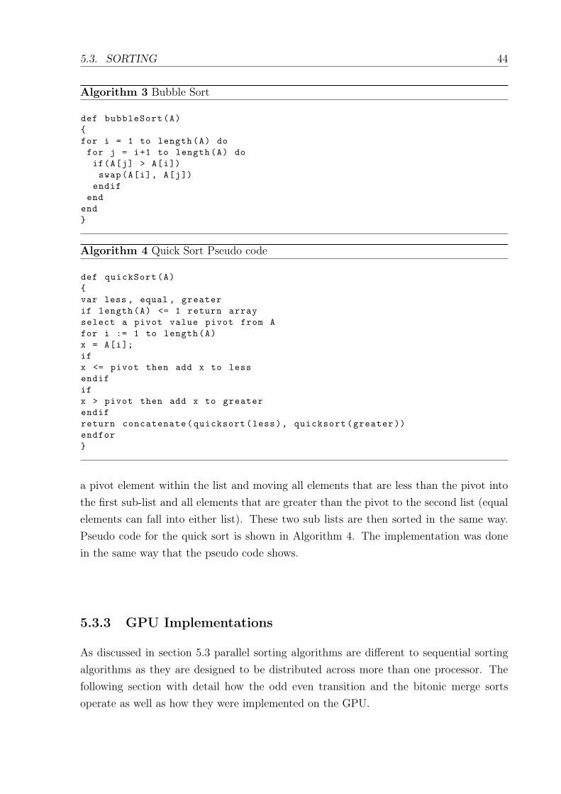
5.3. SORTING 44
Algorithm 3 Bubble Sort
def bubbleSort(A){for i = 1 to length(A) dofor j = i+1 to length(A) doif(A[j] > A[i])swap(A[i], A[j])
endifend
end}
Algorithm 4 Quick Sort Pseudo code
def quickSort(A){var less , equal , greaterif length(A) <= 1 return arrayselect a pivot value pivot from Afor i := 1 to length(A)x = A[i];ifx <= pivot then add x to lessendififx > pivot then add x to greaterendifreturn concatenate(quicksort(less), quicksort(greater ))endfor}
a pivot element within the list and moving all elements that are less than the pivot intothe first sub-list and all elements that are greater than the pivot to the second list (equalelements can fall into either list). These two sub lists are then sorted in the same way.Pseudo code for the quick sort is shown in Algorithm 4. The implementation was donein the same way that the pseudo code shows.
5.3.3 GPU Implementations
As discussed in section 5.3 parallel sorting algorithms are different to sequential sortingalgorithms as they are designed to be distributed across more than one processor. Thefollowing section with detail how the odd even transition and the bitonic merge sortsoperate as well as how they were implemented on the GPU.

5.3. SORTING 45
Algorithm 5 Odd Even Transition Sort
def transitionSort (){repeat n timesdo in parallelif(element[n] > element[n+1])swap(element[n], element[n+1)endifend parallelend}
Odd Even Transition Sort
The odd even transition sort is based on the operation of the bubble sort described in 5.3.2[20]. The operation of the sort considers every element to the left of itself and comparesand swaps them as necessary. As this is a parallel sorting algorithm there is no explicitloop. In fact the algorithm is best thought of as a network where the nodes in the networkperform the compare-swap operation on the elements in question and data moves with inthe network until it is sorted. The parallel pseudo code for the odd even transition sortis presented in Algorithm 5.
The odd even transition sort was implemented in a single fragment shader using the renderto texture feedback loop mechanism describe in sub-section 5.3.5. The compare andexchange operations were performed within a fragment shader. This shader’s executionrepresented one pass of the algorithm. The actual data values were encoded into the redcolour channel of a texture with the same dimensions as the data set size. In order toinvoke the shader to execute on the data a screen sized quad was rendered to the screen.The resulting image in the frame buffer was then read back in the texture and re-renderedinvoking another pass of the algorithm. This procedure was repeated n times resulting inthe data being fully sorted. The images in figure 5.6 shows the data being sorted at variousstages during the execution of the algorithm. It should be notes that the data, althoughdepicted in a two dimensional sense is actually representative of a linear sequence.

5.3. SORTING 46
Figure 5.6: Odd Even Transition Sort
Bitonic Merge Sort
A bitonic merge sort is another sorting network. It operates on the principal of bitonicsequences.
A bitonic sequence is composed of two sub-sequences, one monotonically non-decreasingand the other monotonically non-increasing. Bitonic sequences have two properties thatare of importance in a bitonic merge sort. The first is that a bitonic sequence can bedivided in half and produce two sequences such that both are bitonic. The second isthat either every element in the first sequence is less than or equal to every element inthe second sequence or every element in the first sequence is greater than or equal toevery element in the second sequence. A sorted sequence is a bitonic sequence whereone of the comprising sequences is empty. In order to perform this division, elements incorresponding positions in each sequence are compared and exchanged as necessary. Thisoperation is sometimes called a bitonic merge [24, 21]. In order to perform a full bitonicmerge sort the initial sequence is assumed to have length a power of two. This ensuresthan it can be continually divided in half. The first half of the sequence is sorted intoascending order while the second half is sorted into descending order. This operationresults in a bitonic sequence. A bitonic merge is performed on this sequence to yield twobitonic sequences each of which is sorted recursively until all the elements in the sequenceare sorted. The pseudo code in Algorithm 6 presents the recursive algorithm for a bitonicmerge sort.
The implementation of the bitonic merge sort was significantly more complex than the oddeven transition sort. The shaders represented the bitonic merge operation while the sortmerge function was performed implicitly by passing a uniform parameter to the shader

5.3. SORTING 47
Algorithm 6 Bitonic Merge Sort
def bitonicMergeSort(int [] A, int n){perform_bitonic_merge ()sort_bitonic(A,n/2)sort_bitonic(A+n/2,n/2)
}
Figure 5.7: Bitonic Merge Sort
indicating the current recursive depth. As with the odd even transition sort describedin sub-section 5.3.3 the data values of the list were encoded into the red channel of atexture and the same render to text mechanism was used to perform the log2n iterationsnecessary to sort the data fully. The images in figure 5.11 show the data being sorted atvarious stages during the execution of the algorithm. Once again it should be notes thatthe data is actually a one dimensional sequence, not two dimensional.
5.3.4 Difficulties Encountered
There were a number of difficulties encountered in implementing sorting on the GPU.This sections details various salient difficulties that presented themselves during the im-plementation, some of which were referenced to earlier. It also provides caveats and waysin which the problems could be solved and circumvented.
5.3.5 Render to texture
Sorting is a multiphase operation and can only be accomplished through a number ofiterations. Therefore there is a need for a feedback loop where data that has been operated

5.3. SORTING 48
Figure 5.8: Render to Texture Feedback Loop
T e x t u r e V e r t e x S h a d e r F r a g m e n t S h a d e r O f f s c r e e n B u f f e r
R e a d - b a c k t o T e x t u r e
on is passed back to the beginning of the sorting operations and used in the next iteration.This need extends beyond sorting and applying to graphics processing in a general sense.The simplest approach to creating this feedback loop is rendering to a texture. This isachieved by rendering normally to the the off screen frame buffer, but then instead ofswapping the buffers to display the rendered data result, the contents of the off screenframe buffer are read out, and copied directly back into the source texture and the buffercleared. This means that the operation of all the shaders takes place on the texture data,and the resulting data is stored in the texture again ready for another iteration. Whichcan be initiated by rendering more geometry. Figure 5.8 illustrates this process.
5.3.6 Coordinate Wrapping
This is the same problem that manefested itself in the searching algorithms in sub-section5.4.2 where the entire grid need to be considered as a single list.
5.3.7 Uniform Parameters
Sorting requires information to be passed into the kernel programs. In the bitonic mergesort, the step size and current recursive depth needed to be known within the executionenvironment of the fragment shader in performing the bitonic merge operation. Theseparameters are bound to the kernel program from the housing C++ program and theyappear and are accessible as standard parameters in the shader.
5.3.8 Results
Table 5.7 presents the mean execution times of the four different sorting operations acrossthe different data set sizes.

5.3. SORTING 49
Table 5.7: Mean Execution Times of Sorting Algorithms (µs)
Size Bubble Quick Transition Bitonic Merge32 1,245.34 119.29 7824.04 2418.9364 94,456.92 508.88 10544.65 2886.15128 1,656,493.37 2179.00 11345.21 2998.27256 21,266,453.67 9419.59 15452.44 3156.21512 2,988,593,594.34 40954.87 18546.23 5360.471024 48,651,723,523.47 178791.31 23681.59 6022.12
Figure 5.9: Sorting Algorithm Execution Times
Bubble.Sort Quick.Sort Transition.Sort Bitonic.Merge.Sort
32x3264x64128x128256x256512x5121024x1024
Sorting Algorithms
Log
Exe
cutio
n T
ime
in M
icro
seco
nds
(ms)
05
1015
2025
These execution times are presented visually in figure 5.9. It should be noted that thetimes are presented on a log scale.
5.3.9 Performance Analysis
The execution times depicted in figure 5.9 conform accurately to the predicted complex-ities in table 5.6. There are several salient points to notice in comparing sorting on theGPU and sorting on the CPU. The CPU sorts out perform the GPU’s for the smaller testcases in general. The reason for this is the structure of the feedback loop. As discussedin sub-section 5.3.5 the feedback loop is constructed by copying the contents of the frame

5.3. SORTING 50
Table 5.8: Relative Speedup of GPU Sorting Algorithms to Quick SortSize Relative Speedup Factor
Transition Sort Bitonic Merge Sort32 0.02 0.0564 0.05 0.18128 0.18 0.75256 0.61 2.98512 2.21 7.641024 7.55 29.69
buffer back into the texture. This an expensive operation and the GPU implementationspay the price on the smaller data set. However as the data set size increases the parallelnature of the GPU based algorithms offset the cost of the render to texture operationand outperform the CPU sorts. This is illustrated in table 5.8 where the speedup of thetransition and merge sorts in computed against the faster of the CPU sorts, the quick sort.The bubble sort is excluded from this comparison as is it infeasible for large data sets andgenerally only considered in sorting because of its simplicity and not it’s efficiency. Theactual speedups of the odd even transition sort and bitonic merge sorts were computedas:
STransitionSort =µQuicSort
µTransitionSort
SMergeSort =µQuicSort
µMergeSort
Considering sorting performance as a whole. The average execution time for the CPUquick sort and GPU bitonic merge sorts across all data set sizes are µQuickSort = 38, 662.16
and µMergeSort = 3, 788.34 respectively. These values can be used to compute an averagerelative speedup of GPU sorting to CPU sorting as:
S =µQuickSort
µMergeSort= 10.23
This shows than on average the GPU performed the sorting operation 10.23 times fasterthan the CPU or in other words exhibited a speed up of 1, 023%. It is also interestingto investigate the performance of the two GPU sorting algorithms independently of theCPU ones. The transition sort has a complexity of O(log2n) where are the bitonic mergesort has a complexity of O(log(n2)). The graphs of these two complexities is shown infigure 5.10 and figure 5.11. It can be seen that these two sorting algorithms both havethe same asymptotic behavior.

5.3. SORTING 51
Figure 5.10: Transition Sort Asymptotic Complexity
0 200 400 600 800 1000
010
2030
40
Input Size
Com
plex
ity
Figure 5.11: Bitonic Merge Sort Asymptotic Complexity
0 200 400 600 800 1000
02
46
810
1214
Input Size
Com
plex
ity

5.3. SORTING 52
Table 5.9: Bitonic Merge Sort with Varying Numbers of Shader Cores
Cores Mean Execution Time (µs)4 28644.768 10863.3924 3788.34
Figure 5.12: Mean Execution Time with Different Numbers of Cores
4 8 24
Shader Cores
Mea
n E
xecu
tion
Tim
e (m
icro
seco
nd)
050
0010
000
1500
020
000
2500
0
Since the GPU is a parallel processor and the algorithms being analyzed are parallel innature it is important to consider the effect that the number of shaders cores has on theperformance. It is expected that where a GPU has more shader cores the performance ofthe sorting algorithm distributed better and executes faster. Table 5.7 shows that this isindeed the case as with a higher number of shaders cores the performance increases, thisinformation is presented graphically in figure 5.13.
5.3.10 Optimizations
As stated in section 5.3.1 the implementations where constructed to be canonical andgeneral in nature. With no specific optimizations made. This section will detail what

5.4. SEARCHING 53
types of optimization could be made to the GPU based sorts to increase performanceeven further.
5.3.10.1 Feedback Mechanism
As mentioned in 5.3.5 the feedback loop structure introduces a large performance bot-tleneck as moving data back from the CPU to texture memory is slow. A number ofmechanisms have been developed to remove this bottleneck. A possibly optimal way ofrendering directly into a texture without the need to copy data between memory loca-tions. This method is not standardized in OpenGL 1.3 however ARB extensions makesit possible [30].
5.3.10.2 Data Encoding
The implementation section detailed that the data to be sorted was encoded in the redchannel of the texture. This leaves the blue, green and alpha channels of the texture totallyunused. If data was encoded in these channels as well, the GPU sorting algorithms couldsort four times more data concurrently with little extra computation incurred.
5.4 Searching
Searching is a well understood area of computer science and involves determining whethera certain element is contained within a list. There are a number of different searchingalgorithms with different speeds. The binary search is one of the the fastest standardsearching algorithms and also the most common in practice if the data being searched issorted. Conversely the linear search is very simple to implement but is slower than thebinary search. The binary and linear searches are the two searching algorithms that willbe investigated in this section. Table 5.10 shows the complexity of these two searchingalgorithms. Thus this section is different from the others as is allow parallel sortingalgorithms to be implemented directly instead of emulating sequential ones on the GPUlike in the searching section.

5.4. SEARCHING 54
Table 5.10: Searching Algorithms
Algorithm ComplexityLinear Search O(n)Binary Search O(log n)
Algorithm 7 Linear Search Pseudo Code
def linearSearch(int [] A, int n, int e){int p = -1;for i := 1 to length(A)if(A[i] == e)p = ireturn p;
}
5.4.1 Approach
In order to analyze the performance of searching using GPGPU both the linear and binarysearches were implemented on the CPU and the GPU. The following section explains theimplementations.
CPU Implementation
A linear search is achieved by iterating through the list and comparing each element toone being searched for. The list was initialized with random data in the range [0..255].Pseudo code to achieve this is shown in algorithm 7.
The binary search algorithm operates by dividing the search space in half each time toisolate the element being searched for. For this reason the binary search operates on alist of already sorted elements. Pseudo code is shown in algorithm 8.
GPU Implementation
The linear search was implemented in exactly the same way as for the CPU except that itwas contained within a shader. The code listing for the shader is presented in AppendixA.3.1.

5.4. SEARCHING 55
Algorithm 8 Binary Search Pseudo Code
def binarySearch(int [] A, int e, int low , int high){while(low < high){int mid = low + (high - low) / 2;if(A[mid] > e){high = mid}if(A[mid] < e){low = mid}if(A[mid] == e)return mid;}return -1;
}
The binary search was implemented in a similar way to the CPU implemented except thatonce again it was housed entirely in a fragment shader. The source code for the binarysearch is presented in Appendix A.3.2.
For both searching algorithms the elements representing the list were random numbersin the range [0.255] encoded in the red channel of the texture in non-decreasing order.In order to invoke the execution of the binary search a 1-by-1 simple quad was rendered.The reason for rendering a 1-by-1 quad was that the fragment shader should only becalled once for the search. Since it is called for every fragment it needs to be ensuredthat there is just a single fragment. A 1-by-1 quad ensures that there is only one callto the fragment shader to perform the search. Ultimately the number of pixels drawndetermines the number of searches executed [20].
5.4.2 Difficulties Encountered
Implementing Gather
Once again the problem appeared of reading data from other texture coordinates otherthan the ones bound. The solution to this problem was to implement gather. This wasdiscussed in sub-section 5.2.2.

5.4. SEARCHING 56
Table 5.11: Mean Search Execution TimesSize Linear Search CPU Binary Search CPU Binary Search GPU Linear Search GPU32 6.34 53.13 349.05 65.5864 16.18 59.26 351.03 172.70128 68.18 66.92 373.34 841.70256 260.15 93.81 383.69 3471.77512 1036.37 160.11 521.59 11061.361024 4184.22 224.51 625.96 32043.02
Single List
Although the data is single list of elements it was stored in a two dimensional repre-sentation in a texture. Thus care needed to be taken when addressing other elementsas they could lie on a different row of the texture. The problem was circumvented byimplementing boundary checks on all non-local comparisons.
5.4.3 Results
The run times for the various searches on the different data sets is shown in table 5.11.
These results are also graphed in figure 5.13.
5.4.4 Performance Analysis
It can be seen that the GPU searches, although comparable to the CPU searches is notfaster. The reason for this is the fact that is is only being executed once in one instanceof a fragment shader. As mentioned in sub-section 5.5.1.1 in order to invoke one searchone fragment shaders needs to be executed which in turn requires a single pixel. Thismeans that the benefits of the parallel processing architecture are wasted and there isno potential speedup available as the clock speed of a CPU a lot higher than that of aGPU. From this it is expected that the performance of the search stay relatively constantwith differing numbers of shader cores. Table shows that this is indeed the case and themean execution time varies too a smaller degree than seen in previous implementationslike sections 5.1 and 5.2. Also the variance that does occur is mostly attributed to thespeed of the cores rather than the number.

5.4. SEARCHING 57
Figure 5.13: Mean Execution Time of Searching Algorithms
CPU Linear CPU Binary GPU Binary GPU Linear
Data set size
Log
Mea
n E
xecu
tion
time
(mic
rose
cond
s)
02
46
810
Table 5.12: Relative Speedup of CPU to GPU Binary Searches
Size CPU Binary Search GPU Binary Search Relative Speedup32 53.13078 349.049 0.1564 59.25634 351.030 0.17128 66.92092 373.343 0.18256 93.80865 383.698 0.24512 160.10641 521.592 0.311024 224.51239 625.962 0.36

5.4. SEARCHING 58
Table 5.13: Mean Performance on Shader CoresCore Mean Execution Time
4 4689.498 4604.1424 3872.71
Table 5.12 gives the relative speedup of the CPU to GPU implementations for increasingdata set sizes, computed as:
S = µCPU
µGPU
It can be seen from these results that the CPU outperforms the GPU by increasingly largermargins as the data set increases. Once again the reason for this can be attributed to thefact that the GPU cannot utilize its parallel architecture and thus is on an architecturalpar with the CPU and, because of the CPU’s optimization for elementary sequentialprocessing constructs, like loops, can perform the calculations much faster than the GPUcan.
The weak performance of the GPU searches lie in the fact that it is the algorithms areatomic in the sense that they are not being paralleled and distributed across more thanone processor. For this reason the execution of the algorithm is contained entirely within asingle shaders and executes in one go as on a sequential processing architecture. Althoughthe GPU performs quite comparably to the CPU it is still slower for this reason.
5.4.5 Optimizations
This implementation has room for extension to perform parallel searches. Since renderinga single pixel equates to performing a search, a number of pixels could instead be renderedand although this would not increase the speed of the seaches it would allow a number ofsearches to be executed in parallel.

5.5. AES ENCRYPTION 59
Table 5.14: Key-Block-Round Combinations
Type Key Length (words) Block Size (word) Number of RoundsAES-128 4 4 10AES-192 6 4 12AES-256 8 4 14
Algorithm 9 AES Encryption Pseudo Code
KeyExpansionInitial RoundAddRoundKeyfor(i = 1 to Rounds -1){SubBytesShiftRowsMixColumnsAddRoundKey}SubBytesShiftRowsAddRoundKey
5.5 AES Encryption
Advanced Encryption Standard (AES) [11] is a symmetric key cryptographic algorithmalso known as Rijndael. The AES algorithm is a symmetric block cipher that can encrypt(encipher) and decrypt (decipher) information. Encryption converts data to an unintel-ligible form called cipher text; decrypting the cipher text converts the data back into itsoriginal form, called plain text [2]. Most of AES calculations are done in a special mathe-matical finite field [12]. AES takes as input the block of plain text to encrypt along witha specified key. The encryption algorithm takes the form of a variable number of rounds,each comprised of a number of operates that takes place in sequence to encrypt the data.Decryption is performed in a similar way. AES can operate in a number of forms, varyingthe data block size, key size and number of rounds. Table 5.14 shows the different typesof AES [2]. AES-128 was used because it is the most canonical form of the algorithm aswell as the fact that it is simplified by the restriction of a power of 2 block size.
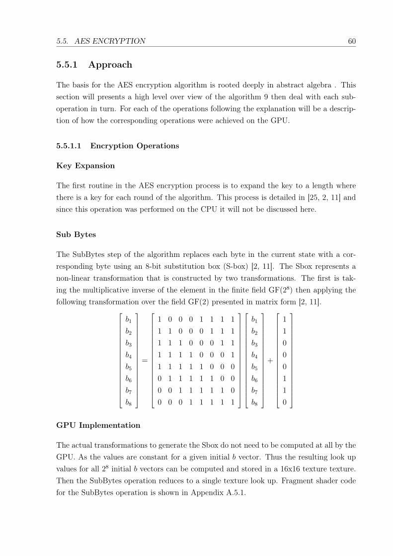
5.5. AES ENCRYPTION 60
5.5.1 Approach
The basis for the AES encryption algorithm is rooted deeply in abstract algebra . Thissection will presents a high level over view of the algorithm 9 then deal with each sub-operation in turn. For each of the operations following the explanation will be a descrip-tion of how the corresponding operations were achieved on the GPU.
5.5.1.1 Encryption Operations
Key Expansion
The first routine in the AES encryption process is to expand the key to a length wherethere is a key for each round of the algorithm. This process is detailed in [25, 2, 11] andsince this operation was performed on the CPU it will not be discussed here.
Sub Bytes
The SubBytes step of the algorithm replaces each byte in the current state with a cor-responding byte using an 8-bit substitution box (S-box) [2, 11]. The Sbox represents anon-linear transformation that is constructed by two transformations. The first is tak-ing the multiplicative inverse of the element in the finite field GF(28) then applying thefollowing transformation over the field GF(2) presented in matrix form [2, 11].
b1
b2
b3
b4
b5
b6
b7
b8
=
1 0 0 0 1 1 1 1
1 1 0 0 0 1 1 1
1 1 1 0 0 0 1 1
1 1 1 1 0 0 0 1
1 1 1 1 1 0 0 0
0 1 1 1 1 1 0 0
0 0 1 1 1 1 1 0
0 0 0 1 1 1 1 1
b1
b2
b3
b4
b5
b6
b7
b8
+
1
1
0
0
0
1
1
0
GPU Implementation
The actual transformations to generate the Sbox do not need to be computed at all by theGPU. As the values are constant for a given initial b vector. Thus the resulting look upvalues for all 28 initial b vectors can be computed and stored in a 16x16 texture texture.Then the SubBytes operation reduces to a single texture look up. Fragment shader codefor the SubBytes operation is shown in Appendix A.5.1.

5.5. AES ENCRYPTION 61
ShiftRows
The shift rows operation cycles the bytes in each row a variable amount. The first row isnot shifted, then second row is shifted cyclically left one position, the third row two andfinally the forth row three positions.
GPU Implementation
The shift operation is simple to perform on the GPU. It can be achieved by offsetting thecurrent fragment shaders texture coordinates based it row (y-position) and performing asingle texture look up on it’s own texture. Code for achieving this if given in AppendixA.5.2.
MixColumns
The MixColumns operation operates on each of the four columns of the state. Each columnof the state is representative of a four-term polynomial over GF(28), this polynomial ismultiplied modulo x4 + 1 with the fixed polynomial a(x), given by:
a(x) = {03}x3 + {01}x2 + {01}x1 + {02}
GPU Implementation
Unfortunately this operate cannot be performed using a look up table as in 5.5.1.1. Asthe state is large so the actual multiplication needs to be performed. The multiplicationis simple to perform and uses a number of the bitwise logical operations like AND, OR,and XOR. The problem is that shader languages like Cg do not have support for logicaloperations [13]. Although reservation has been made for the corresponding symbols &, |and ^ [13], they have not been implemented yet. This introduced a large problem as tohow a seemingly simple bitwise operations like AND, OR and XOR could be performed.Section 5.5.2 deals thoroughly with how this problem was solved and once implementationthe multiplication can be performed as is would be on a sequential processor, the fragmentshader code for the MixColumns operation is given in Appendix A.5.3.
AddRoundKey
The AddRoundKey operation simply XORs the current RoundKey with the state.

5.5. AES ENCRYPTION 62
GPU Implementation
As seen in sub-section what should be a trivial operation turns out to be quite complexwithout the functionality of logical bitwise operators in the shader language. Sub-section5.5.2 shows how the XOR operation was implemented. Once achieved the AddRoundKeyoperation can be performed by XORing elements of the state with the corresponding ele-ments of the current key. Appendix A.5.4 gives the code for the AddRoundKey operation.
With each of the operations of AES implemented, the whole encryption process can beachieved by encoding the initial state and expanded round key (see sub-section 5.5.1.1)into textures. A 4-by-4 pixel quad was then rendered to the screen with the initialSubBytes fragment shader bound. This produced the output for the first stage of theAES encryption. The content of the frame buffer were then copied back into the textureusing the render to texture feedback mechanism that was described in sub-section 5.3.5after which the ShiftRows fragment shader was loaded and another 4-by-4 pixel quadrendered. This process was repeated for the MixColumns and AddRoundKey operationsto yield an iteration of the AES encryption. Since ten iterations were required the wholeprocess is preformed 10 times giving the encrypted state. Care was taken to treat thefinal iteration correctly, since the AddRoundKey operation does not take place here.
5.5.2 Difficulties Encountered
Implementing Bitwise Operations on the GPU
As mentioned in sub-sections 5.5.1.1 and 5.5.1.1 the Cg language does not currentlyimplement bitwise operators. This makes a seemingly trivial task like a logical XORimpossible to perform without some other mechanism in place. In order to provide thisfunctionality, which was needed to perform the AES Encryption, a look up table of valueswas precomputed and stored in a texture. The texture was 256 x 256 and its red, greenand glue colour channels corresponded to the XOR, OR and AND operations. These areall binary operators and the x and y indices into the texture correspond to the operandsand the values stored in each channel to the resulting binary operations value. In orderto use this mechanism to perform logical binary operations the texture was bound to thefragment shaders that required this functionality. Then when an operation needed to beperformed the two operands were scaled to the texture coordinate range of [0.0..1.0] anda dependent texture look up was performed on the texture. The resulting colour channelcould then be read to give the XOR, OR or AND or the operands respectively. Figures5.14, 5.16 and 5.15 depict visually the red, green and blue channels respectively. The

5.5. AES ENCRYPTION 63
Figure 5.14: XOR Look up Field
Table 5.15: AES Encryption Single BlockType Average Number of Encryptions per SecondCPU 3125.76GPU 626.24
limitation of this implementation is the range of values of the operands. Since a 256 x 256textures was used only values within this ranges could be computed. Since AES operatesin this ranges of value, these constraints are not a problem.
5.5.3 Results
Tables 5.15 and 5.16 show the average number of complete AES encryptions that couldbe performed on both the CPU and GPU when encrypting one and many blocks per cyclerespectively.
Table 5.16: AES Encryption Multi BlockType Average Number of Encryptions per SecondCPU 7254.25GPU 25449.65

5.5. AES ENCRYPTION 64
Figure 5.15: AND Look up Field
Figure 5.16: OR Look up Field

5.5. AES ENCRYPTION 65
5.5.4 Performance Analysis
The results in table 5.15 show that the CPU out-performs the GPU by a factor of 4.99on the single block encryption test. This value was computed as:
S = µCPU
µCPU= 3125.76
626.24= 4.99
This result is not surprising as no parallelism is being taken advantage of in the GPUimplementation and since the CPU is optimized for this type of sequential processing, itis hard to beat.
Rendering 16 pixels each render cycle is a waste of graphics processing power. It wasdetailed in section 3.3 that the stream processing models is effective with contiguousstreams of similar data. By increasing the size of the view port to a larger size andrendering more than one state in a render cycle parallelism is exposed that yield theencryption rates shown in table 5.16.
Figure 5.17 shows the results of the CPU and GPU implementations of AES Encryptionwith increasing number of states being encrypted per cycle. The red plot is the GPUimplementation where as the blue plot is the CPU one. There is a lot of interestinginformation contained in this result. Firstly it can be seen that the GPU AES Encryptionimplementation out-performs the CPU implantation by a large margin. The reason for thisis the fact the where as in the single block test only a single 16 byte state was encryptedper cycle. Now using a view port of 256 x 256 the 4 x 4 states are tilled across it andprocessed in parallel. This allowed for 4096 times more data to be encrypted per cycle.The CPU encryption rate plot showed expected results. Since it is a sequential processor,it cannot be expected to gain large speedup from processor more data per cycle. As aresult processing more data per cycle results in a slower cycle time which balances out,yielding almost constant encryption rates across block size. Table 5.17 shows the meanencryption rate using all block sizes. This result clearly shows the effect of concurrentlyprocessing blocks, and when compared to table 5.15 it can be seen that where the CPUonce outperformed the GPU by a factor of 4.99, the GPU now outperforms the CPU by2.87 times. Considering the fastest results of both the CPU and GPU implementationsin table 5.18 the GPU performs even better now outperforming the CPU by 5.17 times.Figure 5.17 seems to imply that more block with yield even higher encryption rates.Unfortunately there is a limit to the size of the renderable surface while maintaining a 1to 1 aspect ratio. This is a common platform limitation of screen resolution in operatingsystems. This problem can be circumvented in a number of ways by these methods arenot general.

5.5. AES ENCRYPTION 66
Figure 5.17: AES Multi-Block Encryption Rate
0 20 40 60 80 100 120
020
0040
0060
0080
0010
000
1200
0
Encryptions per Cycle
Enc
rypt
ion
Rat
e (K
b/s)
Table 5.17: Mean Encryption Rate
Type Mean Encryption Rate (Mb/s)CPU 1.553GPU 4.457

5.6. RENDERING FRACTAL IMAGES 67
Table 5.18: Maximum Encryption Rate
Type Encryption Rate (Mb/s)CPU 2.32GPU 12.00
By packing more that one state to be encrypted into one single rendering cycle the GPU isable to take advantage of the per-routine parallelism and gain large performance increasesover the CPU.
5.6 Rendering Fractal Images
A fractal is a self referential image. Fractals exist in a number of forms. This implemen-tation is concerned with the generation of fractal images in regions of the complex plane.More specifically the Mandelbrot fractal of the Julia fractal set. Rendering a fractal im-age involves determining, within a region of the complex plane, which set of point in thatregion are contained in the fractal set and which are not. Unfortunately to determinethis accurately requires infinite sequence arithmetic and for this reason approximationsare usually used. Mathematically the Mandelbrot set is defined as the set of all pointswhose magnitude is bounded by |2| under the recurrence relation:
Zn = Z2n−1 + C
where Z0 = 0, and all numbers are complex.
5.6.1 Approach
In order to investigate GPGPU’s applications to fractal rendering the processing of therecurrence relation was offloaded into a fragment shader instead of being done on theCPU. A screen sized quad was then rendered which resulted in the fragments of the quadthat were contained in the mandelbrot set being coloured, while the remainer were leftblank. The code for achieving this is given in Appendix A.7.1. This same code wasimplemented for the CPU in order to make performance comparisons.
Testing was conducted and a 512-by-512 area of the complex plane, with the magnitudeof the recurrence relation tested for escape over 2048 iterations.

5.6. RENDERING FRACTAL IMAGES 68
Table 5.19: Fractal Rendering SpeedsType Average Frames Per SecondCPU 2.12GPU 7.83
Table 5.20: Mandelbrot Fractal Computation Rate (points/s)Type RateCPU 555,745.28GPU 2,052,587.52
5.6.2 Difficulties Encountered
Numerical Precision
As the view is zoomed in the area of the complex plane being displayed becomes smallerand smaller. In order to accurately render the complex plane at higher magnificationssmall point intervals need to be used. This becomes inaccurate at very high magnificationand precision is lost yielding pixelated images. This problem could be overcome with theuse of a high precision floating point division strategy. However Cg currently does nothave support for this.
5.6.3 Results
Table 5.19 shows the average number of complete renders per second on the GPU andCPU implementations. Table 5.20 gives the average number of points in the complexplane processed per second. The image set in figure 5.18 set shows a collection of variousregionr of the Mandelbrot fractal.
5.6.4 Performance Analysis
Computing the relative speedup of the GPU implementation as
S = µCPU
µGPU= 7.83
2.12= 3.69
This shows that the GPU outperforms the CPU implementation by a factor of 3.69, or inother words executes 369.00% faster. This speed is not surprising after previous results

5.7. CELLULAR AUTOMATA SIMULATION ON A GRID 69
Figure 5.18: Mandelbrot Fractal Images
Table 5.21: John Conway Rule SetCondition Consequence
Occupied cell has 0, 1, 4, 5, 6, 7, or 8 neighbors Organism dies.Occupied cell has 2 or 3 neighbors Organism survives to the next generation.Unoccupied cell has 3 neighbors The cell becomes occupied
that have been seen. Since the contents of the fragment shader operate only on a singlepoint in the complex plane and base computation solely on the point in question thefractal generation processing parallelized well yielding speed ups.
5.7 Cellular Automata Simulation on a Grid
Grid simulations involve iterative processing on an array of elements under some rule setto generate a successive population on the grid. This process is continued to create asimulation. This implementation simulates John Conway’s game of life. Where by thegrid population is initialized randomly. Thereafter at each iteration the rule set in table5.21 is applied.

5.7. CELLULAR AUTOMATA SIMULATION ON A GRID 70
Table 5.22: Cellular Automata Execution TimeType Frames per SecondCPU 42.85GPU 158.45
5.7.1 Approach
The rule set was coded into a shader. A screen sized quad was then rendered for eachiteration of the simulation and the fragment shader was used to process the rule set.the resulting image was then copied back into the initial texture using the Render totexture feedback mechanism from sub-section 5.3.5. The process continued as long as thesimulation was needed to run. Whether a cell was dead or alive was encoded into the redcolour channel where an intensity of 1.0 indicated an alive cell and 0.0 a dead one. A512x512 texture was used creating a simulation grid of the same size.
5.7.2 Difficulties Encountered
5.7.2.1 Boundary Conditions
The only difficulty encountered was with activity at the boundary of the gird. Therewere two approaches to solving this. The first is to wrap the texture coordinates meaningthat neighbors of cell on the boundary of the simulation grid were on the opposite sideof the grid. A second approach was to use the boundary pixel of the grid as a nullcomputation zone where no processing takes place at all. The latter approach was usedin this implementation.
5.7.3 Results
Table 5.22 shows the number of frames per second rendered on the CPU and GPU im-plementations of the cellular automata program.
The image set in figure 5.19 shows the grid simulation in progress.

5.8. SUMMARY 71
Figure 5.19: Cellular Automata Simulation
5.7.4 Performance Analysis
Computing the relative speedup of the GPU implementation as
S = µGPU
µCPU= 158.45
42.85= 3.70
This shows a performance increase of 370%. Also it is a very similar performance ratio tothat seen in the Fractal rendering implementation in section 5.6. This is not surprisingas both problem domain are similar in many regards. The reason for this is because itinvolves the rendering of grid with its composite cells either being displayed or not basedon some function. In the case of the Mandelbrot fractal the function was whether therecurrence relation at the point was bounded. In the case of cellular automata it wasbased on the number of neighbours the cell had and its current state. Effectively theprograms reduce to the constant mapping of a function to a list - something that GPUsperform very well because of the consistency of the operation.
5.8 Summary
Given the results from the implementations it can be seen that there is a board spectrumof speed ups that can be achieved from processing on the GPU. Some specific problems

5.8. SUMMARY 72
exhibit massive speed ups even for small data set sizes like the matrix operations insections 5.1 and 5.2. This is due to the parallel nature of the problem and it formulationon the GPU as independant subroutines that when all performed result in the completedaction. This type of formulation lends itself to a GPU implementation because of thisparallel nature.
Some problems exhibit good performance speed ups but more importantly good asymtoticperformance. This was shown in section 5.3 where CPU implementations outperformedthe GPU for smaller data sets. However as the data set size increased so did the executiontime for the GPU implementation where as the growth of the GPU implementation wasmuch better. This makes GPU a prefereable option for processing depending on the inputsize.
Some problems performed worse on the whole like the searching algorithms in section 5.4.The reason for this was once again the nature of the problem. An atomic problem likea binary search cannot be distributed across multiple processors as easily and effectivelyas the parallel sorting networks in section 5.3. This ultimately lead to a solution wherethe GPU was performing the operations for the searches in exactly the same way as theCPU was. This is an example of an implementation where not exposing some kind ofdata parallelism caused slower execution time.
Excellent performance was gained from the AES implementation in section 5.5. Thiswas not the case initially however as the initial implementation was outperformed by theCPU. Only once the parallelism of the states was identified and taken advantage of did theimplementation start to outperform the CPU. This once again illustrates the importanceof some type of concurrency or parallelism that can be the difference between a poor andeffective GPU implementation.
Finally the graphical simulation in sections 5.6 and 5.7, although more an excercise inoffloading processing from the CPU to the GPU, again showed how performance could begain from taking advantage of GPU resources.
On the whole a lot of information can be gleamed from the implementations and it is opento analysis on a number of depths. The next chapter will use the information that hasbeen presented here in drawning to a conclusion the answers to the research intentionsput forward in section 1.1.

Chapter 6
Discussion and Analysis
This section will drawn on the information gained in the discussion sections of chapter5. Where these sections have dealt independently with the current implementation, thissection will cross correlate results in order to gain a deeper understanding of generalcomputation on graphics processing units. More specifically a plethora of results andcaveats of GPGPU have been brought to the surface and this information can now be usedin answering the questions posed in the intentions of research section 1.1. Furthermorethis section will be concerned with using the information gained to design a model fordeciding plausibility of a GPGPU implementation on the outset of the problem, instead ofhaving to go through the trouble of implementation before seeing if the results are betterthan processing on a CPU.
Viability
GPGPU certainly is a viable option for processing. Technology trends indicate thatgraphics processing power will increase steadily and rapidly in the future. GPGPU willobviously benefit from these advancements
Difficulty
GPGPU is not as simple as constructing a program to execute on the CPU. Insteadit requires experience in a number of languages and APIs. Though there is a lot ofchoice in each, it is still required that the programmer have a good grasp of a high levelprogramming language, graphics API, windowing API and shader language. This adds tothe complexities of the programming as care must be taken to implement things correctlyand accurately across all areas.
73

6.1. GPGPU VIABILITY ANALYSIS MODEL 74
Performance
Performance on the GPU varies with the problems being tackled. Some problems exhibitphenomenal speed ups like the matrix operations where the GPU outperforms and CPUby hundreds of times. Others enjoy speed up to a lesser degree. The searching imple-mentations did not exhibit a speedup and it is important to consider why. The searcheswere implemented atomically in the sense that the were not distributed across more thanone shader core when they were executed. This means that the CPU and GPU imple-mentation were executing in exactly the same way conversely to the matrix operationimplementation for example where the problem could be easily divided into elementaryindependent routines. This result is important and it will serve as a criteria in the analysismodel presented in section 6.1.
6.1 GPGPU Viability Analysis Model
As mentioned earlier it was sought to construct a model by which problems could beevaluated to determine the viability of processing them on the GPU. It is proposed thatthree criteria of the proposed problem be considered:
Arithmetic Intensity
Arithmetic intensity refers to the raw amount of mathematical operations to be performed.GPUs excel at this type of computation and gain performance over the CPU.
Parallelizability
Parallelizability refers to the extent to which the program can be divided into, identical,routines that can be executed concurrently. This then implies that there can be nodependence on the results of another routine’s computation nor the order in which theare computed.
Isolation
Isolation refers to extent that parts of the program need to read or write to other routinesin the program. Communication is achieved through scatter and gather which are inher-ently expensive and where possible should be avoided. A low amount of communicationimplies a high degree of isolation.

6.2. FUTURE WORK 75
Evaluating these three criteria of the problem domain can give a good deep sense ofunderstanding of the viability of using GPGPU to solve the problem instead of having toresolve the issue by trial and error.
6.2 Future Work
Optimization
There is a lot of scope for future work in the field of GPGPU. The implementationsin chapter 5 were designed to be simple and general in nature. This approach is goodfor initial analysis but when performance is needed optimization is important. Most ofthe implementations contained optimization sections where information was presented asto how the problems could be approached to yield better performance. Future work in-cludes implementing these optimizations. With the analysis model in section 6.1 problemscan now be evaluated better on the outset to determine whether they will benefit fromprocessing on the GPU. This allows for more complicated, time consuming and largerscale problems to be tackled without the hit-and-miss strategy of having to implementthe problem on both the CPU and GPU to see which performs best.
SLI Investigation
There is room for more performance analysis using SLI technologies to see what effectit has on performance. This would introduce interesting complexities about distributionand communication and the results would give further insight into the power of GPGPU.
GPGPU Meta-Language
GPGPU requires experience in a number of disciplines of computer science including Com-plexity Theory, Distributed and Parallel Processing, Architecture and Graphics. This canput GPGPU out of reach of the casual programmer as on top of these they require ex-perience in not only a high level language, but also a shader language and knowledge ofa Windowing and Graphics API. Future work could include the design and constructionof a meta-language that will abstract all this from the programmer. The language couldbe used to write a program which a translator could them parse and split into a pro-gram to create and graphical window, the necessary fragment and vertex shaders for thecomputation as well as initializing graphics object like textures to store the information.

6.2. FUTURE WORK 76
Algorithm 10 GPGPU Meta Language
int nums [4]
function mul_two(element i){return i * 2}
<start_gpu_process >
map(mul_two , array)
<end_gpu_process >
display(array)
Consider an example fragment of the meta-language presented in Algorithm 10 whichcould then be parsed to produce an OpenGL program that creates and 2x2 windowswith a 1-to-1 view port aspect ratio. It would also create 2x2 texture called ’nums’. Afragment shader would then also be generated that simply multiplied the colour receivedby two. The OpenGL program would then include code to render a single screen sizedquad to start the computation after which the frame buffer contents were read to displaythe results.

Chapter 7
Conclusion
GPGPU is a powerful resource that has become available to programmers and althoughquite complex to get to grips with, it is a very viable solution to certain computationallyexpensive problems. More specifically problems that exhibit data independance, arith-metic intensity and isolation can gain large performance increases. The implementationsearlier illustrated this well, where some displayed large performance increases of theirCPU counterparts but others were slower.
Graphics developers are well aware of the processing power within their graphics cardsare making this available to programmers both NVIDIAs CUDA framework and ATIsClose-to-Metal interfaces makes general computation available to programmers.
Also the the potential speed up gained is very large if care and thought it put into theimplementation. Graphics processing hardware will continue to become more and morepowerful and a good understanding of how general computation is performed on graphicsprocessing units is key to being able to classify problems that will enjoy faster executiontimes on the GPU. There is a multitude of research that can be done into the fieldof GPGPU and although only an infant field in computer science now is fast growingpopularity and support in industry applications. There is also a lot of scope to take theinformation presented in this paper and go further with it.
77

Bibliography
[1] Amd "close to metal" technology unleashes the power of stream computing.
[2] Federal Information Processing Standards Publication 197.
[3] High level shading language for directx.
[4] Microsoft official website. Online (http://www.microsoft.com).
[5] Moore’s law, the future - technology & research at intel.
[6] Opengl shading language.
[7] Opengl, the industry’s foundation for high performance graphics. Online(http://www.opengl.org).
[8] John Owens Aaron Lefohn, Joe Kniss. Implementing efficient praallel data structureson gpus. In GPU Gems 2, page 521, One Lake Stree, Upper Saddle River, NJ, 2004.Addison Wesley.
[9] Fabio Policarpo Alan H. Watt. Advanced Game Development With ProgrammableGraphics Hardware. A K Leters, Ltd, 2005.
[10] Ian Buck. Taking the plunge into gpu computing. In GPU Gems 2, page 509, OneLake Stree, Upper Saddle River, NJ, 2004. Addison Wesley.
[11] J. Daemen and V. Rijmen, editors. The Design of Rijndael: AES- Advanced Encryp-tion Standard. Springer-Verlag, 2001.
[12] John Durbin. Modern Algebra, An Introduction. Wiley, 1992.
[13] Randima Fernando and Mark Kilgard. The Cg Tutorial. Addison-Wesley Profes-sional, 2003.
[14] James D. Foley. Computer Graphics. Addison-Wesley Professional, 1995.
78

BIBLIOGRAPHY 79
[15] Dominik Göddeke. Gpgpu: Basic math tutorial. 2006.
[16] Kris Gray. DirectX 9 Programmable Graphics Pipeline. Microsoft Press, 2003.
[17] Mark Harris. Mapping conputational concepts to gpus. In GPU Gems 2, page 493,One Lake Stree, Upper Saddle River, NJ, 2004. Addison Wesley.
[18] Rolf Herken. The Universal Turing Machine: A Half-Century Survey. Springer, 1995.
[19] Daniel Horn. Stream reduction operations for gpgpu applications. In GPU Gems 2,page 557, One Lake Stree, Upper Saddle River, NJ, 2004. Addison Wesley.
[20] Peter Kipfer and Rudiger Westermann. GPU Gems 2, chapter 46, pages 733 – 746.Addison Wesley Professional, 2005.
[21] Donal Knuth. The Art of Computer Programming. Addison-Wesley Professional,1998.
[22] David Luebke, Mark Harris, Jens Krager, Tim Purcell, Naga Govindaraju, Ian Buck,Cliff Woolley, and Aaron Lefohn. Gpgpu: general purpose computation on graphicshardware. In SIGGRAPH ’04: ACM SIGGRAPH 2004 Course Notes, page 33, NewYork, NY, USA, 2004. ACM Press.
[23] Ian Buck Mark Harris. Gpu flow-control idioms. In GPU Gems 2, page 547, OneLake Stree, Upper Saddle River, NJ, 2004. Addison Wesley.
[24] Norman Matloff. Introduction to parallel sorting [unpublished]. Department of Com-puter Science University of California at Davis, 2006.
[25] Richard Schroeppel Niels Ferguson and Doug Whiting. A simple algebraic represen-tation of rijndael. In Selected Areas in Cryptography, Proc. SAC 2001, 2001.
[26] John Owens. Streaming architechture and technology trends. In GPU Gems 2, page457, One Lake Stree, Upper Saddle River, NJ, 2004. Addison Wesley.
[27] Randi J. Rost. OpenGL Shading Language. Addison-Wesley Professional, 2006.
[28] R Development Core Team. R: A language and environment for statistical computing.R Foundation for Statistical Computing, Vienna, Austria, 2005.
[29] Tarmo Uustalu Varmo. Vene. Advanced Functional Programming: 5th InternationalSchool. Springer, 2005.
[30] Chris Wynn. Opengl render-to-texture. Technical report, NVIDIA Corporation.

Appendix A
Code Listings
A.1 Matrix Addition
A.1.1 Matrix Addition Routine
struct RET{float4 color : COLOR;};
RET main(float2 n : WPOS , float2 texCoord : TEXCOORD0 , uniform sampler2D aField ,uniform sampler2D bField){RET OUT;float4 S = tex2D(aField , texCoord );float4 T = tex2D(bField , texCoord );OUT.color = S + T;return OUT;
}
A.2 Matrix Multiplication
A.2.1 Matrix Multiplication Routine
struct RET{float4 color : COLOR;};
80

A.3. SEARCHING 81
int toInteger(float num){return floor(num * 256.0);}
RET main(float2 n : WPOS , float2 texCoord : TEXCOORD0 , uniform sampler2D aField ,uniform sampler2D bField){RET OUT;int A[(int)SIZE];int B[(int)SIZE];for(int i = 0; i < (int)SIZE; i++){A[i] = toInteger(tex2D(aField , float2 ((float)i/SIZE , texCoord.y)).x);B[i] = toInteger(tex2D(aField , float2(texCoord.x, (float)i/SIZE )).x);}int T = 0;for(int i = 0; i < (int)SIZE; i++)T += A[i]*B[i];OUT.color.x = float(T) / 256.0;return OUT;
}
A.3 Searching
A.3.1 Linear Search Routine
RET main(float2 texCoord : TEXCOORD0 , uniform sampler2D array1 ,uniform float key){RET OUT;OUT.color = tex2D(array1 , texCoord );for(int i = 0; i < N*N; i++){float4 T = tex2D(convert(i));if(abs(OUT.color.x - key) < 0.005)
{OUT.color = float4 (0.0, 1.0, 0.0, 0.0);}
}return OUT;}

A.3. SEARCHING 82
if(floor(OUT.color.x * 256) == floor(key * 256.0))OUT.color = float4 (0.0, 1.0, 0.0, 0.0);
return OUT;}
A.3.2 Binary Search Routine
#define SIZE 32#define LOGN (13)struct RET{float4 color : COLOR;};float flatten(float2 v, float s){return floor(v.x * s) + floor(v.y * s) * s;}float2 puff(float v, float s){float a = v / s;float b = fmod(v, s);return float2(b / s, a / s);}float Search(float curpos , float stride , float key , uniform sampler2D data){float2 adr2d = puff(curpos , SIZE);float4 s = tex2D(data , adr2d);float dir = (key <= s.x) ? 1.0 : -1.0;return dir * stride + curpos;}float FinalSearch(float curpos , float stride , float key , uniform sampler2D data){float2 adr2d = puff(curpos , SIZE);float4 s = tex2D(data , adr2d);float dir = (key <= s.x) ? 0.0 : 1.0;return dir * stride + curpos;}RET main(float2 texCoord : TEXCOORD0 , uniform sampler2D array1 ,uniform float stride , uniform float key){RET OUT;OUT.color = tex2D(array1 , texCoord );

A.4. SORTING 83
float curpos = stride;for(int i = 0; i < LOGN -1; i++){stride = floor(stride * 0.5);curpos = Search(curpos , stride , key , array1 );}curpos = Search(curpos , 1.0, key , array1 );curpos = FinalSearch(curpos , 1.0, key , array1 );float2 n = puff(curpos , SIZE);float4 t = tex2D(array1 , n);if(abs(OUT.color.x - key) < 0.005){OUT.color = float4 (0.0, 1.0, 0.0, 0.0);}return OUT;}
A.4 Sorting
A.4.1 Odd Even Transition Sort Routine
#define EPSI 0.001#define SIZE 512.0#define DELTA (1.0 / SIZE)#define LBND (0.0)#define HBND (1.0)struct RET{float4 color : COLOR;};bool left(float2 v){return (abs(v.x - LBND) < EPSI);}bool right(float2 v){return (abs(v.x - HBND) < EPSI);}bool top(float2 v){return (abs(v.y - HBND) < EPSI);}bool bot(float2 v)

A.4. SORTING 84
{return (abs(v.y - LBND) < EPSI);}bool topRight(float2 v){if(top(v))if(right(v))return true;return false;}bool botLeft(float2 v){if(bot(v))if(left(v)) return true;return false;}float2 nextRight(float2 v){if(topRight(v)) return v;if(right(v)){v.x = LBND;v.y = v.y + DELTA;}else{v.x = v.x + DELTA;}return v;}float2 nextLeft(float2 v){if(botLeft(v)) return v;if(left(v)){v.x = HBND;v.y = v.y - DELTA;}else{v.x = v.x - DELTA;}return v;}

A.4. SORTING 85
RET main(float2 texCoord : TEXCOORD0 , uniform sampler2D array1 ,uniform float oddPass){RET OUT;float4 s = tex2D(array1 , texCoord );int actual = int(texCoord.x * SIZE); // [ actual = {0..512} ]bool oddRow = (actual % 2 == 0);float occi;if(oddRow) occi = 1.0;else occi = -1.0;OUT.color = s;//if(right(texCoord )) // OUT.color = float4 (0.0, 1.0, 0.0, 0.0);// return OUT; //if(occi * oddPass > 0.0){float4 t = tex2D(array1 , nextRight(texCoord ));if(s.x < t.x) OUT.color = s;elseOUT.color = t;}else{float4 t = tex2D(array1 , nextLeft(texCoord ));if(s.x >= t.x) OUT.color = s;else OUT.color = t;}return OUT;}
A.4.2 Bitonic Merge Sort Routine
#include "defines.h"struct RET{float4 color : COLOR;};float flatten(float2 v, float s){return floor(v.x * s) + floor(v.y * s) * s;}float2 puff(float v, float s){float a = v / s; float b = fmod(v, s);return float2(b / s, a / s);

A.5. AES ENCRYPTION 86
}RET main(float2 texCoord : TEXCOORD0 , uniform sampler2D array1 ,uniform float stage , uniform float stepno , uniform float offset){RET OUT;float4 s = tex2D(array1 , texCoord );float actual = flatten(texCoord , SIZE);half csign = (fmod(actual , stage) < offset) ? 1 : -1;half cdir = (fmod(floor(actual/stepno), 2) == 0) ? 1 : -1;float gamma = (actual + csign*offset );float2 next = puff(gamma , SIZE);float4 t = tex2D(array1 , next);float4 cmin = (s.x < t.x) ? s : t;float4 cmax = (s.x > t.x) ? s : t;if (csign == cdir) OUT.color = cmin;elseOUT.color = cmax;return OUT;}
A.5 AES Encryption
A.5.1 SubBytes Routine
float Sbox(int A, sampler1D sboxField){float Af = (float)A / 256.0;float4 Sf = tex1D(sboxField , Af);return Sf.x;}RET main(float2 n : WPOS , float2 texCoord : TEXCOORD0 ,uniform sampler2D aField , uniform sampler1D sboxField){RET OUT;int value = floor(tex2D(aField , texCoord ).x * 256.0 - 1.0/256.0);OUT.color.x = Sbox(value , sboxField );return OUT;}
A.5.2 ShiftLeft Routine
float shiftLeft(float2 P, sampler2D aField){

A.5. AES ENCRYPTION 87
int Y = floor(P.y * 4.0);int X = floor(P.x * 4.0);Y = (Y + X) % 4;float Re = (float)X/4.0;float Ce = (float)Y/4.0;return tex2D(aField , float2(Re, Ce)).x;}
A.5.3 MixColumns Routine
float4 mixColumns(float4 R, uniform sampler2D andField ,suniform sampler2D xorField){float4 B, K, H, A = R;
H.x = AND(toInteger(R.x), 128, andField );H.y = AND(toInteger(R.y), 128, andField );H.z = AND(toInteger(R.z), 128, andField );H.w = AND(toInteger(R.w), 128, andField );
B.x = subProcess(R.x, (toInteger(H.x) == 128));B.y = subProcess(R.y, (toInteger(H.y) == 128));B.z = subProcess(R.z, (toInteger(H.z) == 128));B.w = subProcess(R.w, (toInteger(H.w) == 128));
if(toInteger(H.x) == 128)B.x = XOR(toInteger(B.x), 27, xorField );
if(toInteger(H.y) == 128)B.y = XOR(toInteger(B.y), 27, xorField );
if(toInteger(H.z) == 128)B.z = XOR(toInteger(B.z), 27, xorField );
if(toInteger(H.w) == 128)B.w = XOR(toInteger(B.w), 27, xorField );
float4 Ta, Tb, Tc;
Ta.x = XOR(toInteger(B.x), toInteger(A.w), xorField );Ta.y = XOR(toInteger(B.y), toInteger(A.x), xorField );Ta.z = XOR(toInteger(B.z), toInteger(A.y), xorField );Ta.w = XOR(toInteger(B.w), toInteger(A.z), xorField );

A.6. LOGICAL OPERATION ROUTINE 88
Tb.x = XOR(toInteger(B.y), toInteger(A.z), xorField );Tb.y = XOR(toInteger(B.z), toInteger(A.w), xorField );Tb.z = XOR(toInteger(B.w), toInteger(A.x), xorField );Tb.w = XOR(toInteger(B.x), toInteger(A.y), xorField );
Tc.x = XOR(toInteger(Ta.x), toInteger(Tb.x), xorField );Tc.y = XOR(toInteger(Ta.y), toInteger(Tb.y), xorField );Tc.z = XOR(toInteger(Ta.z), toInteger(Tb.z), xorField );Tc.w = XOR(toInteger(Ta.w), toInteger(Tb.w), xorField );
K.x = XOR(toInteger(Tc.x), toInteger(A.y), xorField );K.y = XOR(toInteger(Tc.y), toInteger(A.z), xorField );K.z = XOR(toInteger(Tc.z), toInteger(A.w), xorField );K.w = XOR(toInteger(Tc.w), toInteger(A.x), xorField );
return K;}
A.5.4 AddRoundkey
float addRoundKey(float2 P, sampler2D aField , sampler1D keyField ,sampler2D xorField , float offset){float base = (offset + floor(P.y * 4.0) * 4.0 + floor(P.x * 4.0)) / 256.0;int H = (floor)(tex1D(keyField , base).x * 256.0);int K = (floor)(tex2D(aField , P).x * 256.0);return XOR(K, H, xorField );}
A.6 Logical Operation Routine
float4 logicalOperation(int A, int B, sampler2D logicalField){float Af = (float)A / 256.0;float Bf = (float)B / 256.0;float4 Sf = tex2D(xorField , float2(Af, Bf));return Sf;//Sf.x == A & B//SF.y == A | B//Sf.z == A ^ B}

A.7. RENDERING FRACTAL IMAGES 89
A.7 Rendering Fractal Images
A.7.1 Mandelbrot Fractal Routine
struct RET { float4 color : COLOR; };RET main(float2 texCoord : TEXCOORD0 , uniform sampler2D decal ,uniform float xpos , uniform float ypos , uniform float zoom){RET OUT;float2 n;float2 c;c.x = xpos - 0.5* zoom + texCoord.x*zoom;c.y = ypos - 0.5* zoom + texCoord.y*zoom;n.x = c.x;n.y = c.y;int i = 0; for(i = 0; i < 2048; i++){float tmp = n.x*n.x - n.y*n.y + c.x; n.y = 2.0*n.x*n.y + c.y;n.x = tmp;if(n.x*n.x + n.y*n.y > 4.0) break;}float k = n.x*n.x + n.y*n.y;if(k < 4.0)OUT.color = float4 (0.0, 0.0, 0.0, 0.0);else OUT.color = float4( 1.0 - (float)i/200.0/2.0 , (float)i/200.0 , 0.0, 0.0);return OUT;}
A.8 Cellular Automata
A.8.1 Grid Simulation Routine
struct RET{float4 color : COLOR;};RET main(float2 texCoord : TEXCOORD0 , uniform sampler2D decal){RET OUT;half4 ns;half4 ds;half2 uv = texCoord.xy;float4 centre = tex2D(decal , texCoord );

A.8. CELLULAR AUTOMATA 90
uv.x = texCoord.x;uv.y = texCoord.y - 1.0/512.0;ns.x = tex2D(decal , uv).y;uv.x = texCoord.x;uv.y = texCoord.y + 1.0/512.0;ns.y = tex2D(decal , uv).y;uv.x = texCoord.x - 1.0/512.0;uv.y = texCoord.y;ns.z = tex2D(decal , uv).y;uv.x = texCoord.x + 1.0/512.0;uv.y = texCoord.y;ns.w = tex2D(decal , uv).y;uv.x = texCoord.x - 1.0/512.0;uv.y = texCoord.y - 1.0/512.0;ds.x = tex2D(decal , uv).y;uv.x = texCoord.x - 1.0/512.0;uv.y = texCoord.y + 1.0/512.0;ds.y = tex2D(decal , uv).y;uv.x = texCoord.x + 1.0/512.0;uv.y = texCoord.y - 1.0/512.0;ds.z = tex2D(decal , uv).y;uv.x = texCoord.x + 1.0/512.0; uv.y = texCoord.y + 1.0/512.0;ds.w = tex2D(decal , uv).y;float cnt = 0.0f; bool valid;valid = (ns.x == 1.0f);if(valid) cnt += 1.0f;valid = (ns.y == 1.0f);if(valid) cnt += 1.0f;valid = (ns.z == 1.0f);if(valid) cnt += 1.0f;valid = (ns.w == 1.0f);if(valid) cnt += 1.0f;valid = (ds.x == 1.0f);if(valid) cnt += 1.0f;valid = (ds.y == 1.0f);if(valid) cnt += 1.0f;valid = (ds.z == 1.0f);if(valid) cnt += 1.0f;valid = (ds.w == 1.0f);if(valid) cnt += 1.0f;OUT.color = centre;if(centre.y == 0.0h){

A.8. CELLULAR AUTOMATA 91
if(cnt == 3.0f)OUT.color = float4 (0.0, 1.0, 0.0, 0.0); }else{if (cnt < 2.0f) OUT.color = float4 (0.0, 0.0, 0.0, 0.0);if (cnt > 3.0f) OUT.color = float4 (0.0, 0.0, 0.0, 0.0);if (cnt == 2.0f) OUT.color = float4 (0.0, 1.0, 0.0, 0.0);if (cnt == 3.0f) OUT.color = float4 (0.0, 1.0, 0.0, 0.0);}return OUT;}