ngmn e. v
TRANSCRIPT

Address:
ngmn e. V.
Großer Hasenpfad 30 • 60598 Frankfurt • Germany
Phone +49 69/9 07 49 98-0 • Fax +49 69/9 07 49 98-41
Recommendation on Base Station Active Antenna System Standards
by NGMN Alliance

Page 2 (55) BASTA Active Antenna White Paper
Version 1.0, 23-Jan-2020
Version: 1.0
Date: 23-January-2020
Document Type: Final Deliverable (approved)
Confidentiality Class: P - Public
Authorised Recipients: (for CR documents only)
Project: BASTA AA
Editor / Submitter: Bruno Biscontini (Huawei)
Contributors: Amphenol Antenna Solutions Ericsson Huawei Kathrein Orange Nokia RFS Telecom Italia Telefonica Vodafone
Approved by / Date: NGMN Board, 27th April 2020
© 2020 Next Generation Mobile Networks e.V. All rights reserved. No part of this document may be reproduced or transmitted in any form or by any means without prior written permission from NGMN e.V.
The information contained in this document represents the current view held by NGMN e.V. on the issues discussed as of the date of publication. This document is provided “as is” with no warranties whatsoever including any warranty of merchantability, non-infringement, or fitness for any particular purpose. All liability (including liability for infringement of any property rights) relating to the use of information in this document is disclaimed. No license, express or implied, to any intellectual property rights are granted herein. This document is distributed for informational purposes only and is subject to change without notice. Readers should not design products based on this document.

Page 3 (55) BASTA Active Antenna White Paper
Version 1.0, 23-Jan-2020
Abstract
The current release of the whitepaper provides recommendations on standards for parameters describing an
Active Antenna Systems (AAS). Specifically, electrical, mechanical and ElectroMagnetic Field (EMF)
exposure related parameters and a format for electronic data exchange are introduced.

Page 4 (55) BASTA Active Antenna White Paper
Version 1.0, 23-Jan-2020
Table of Contents 1 Introduction and Purpose of Document .................................................................................................................... 7
1.1 Preface .............................................................................................................................................................. 7 1.2 Introduction ....................................................................................................................................................... 7 1.3 Interpretation .................................................................................................................................................... 8 1.4 Abbreviations .................................................................................................................................................... 8 1.5 References ....................................................................................................................................................... 9
2 Definitions.................................................................................................................................................................. 11 2.1 Antenna terms ................................................................................................................................................ 11 2.2 AAS definition ................................................................................................................................................. 11 2.3 Antenna Reference Coordinate System ....................................................................................................... 12 2.4 Angular Region............................................................................................................................................... 14 2.5 EIRP ................................................................................................................................................................ 16 2.6 Beam ............................................................................................................................................................... 17 2.7 AAS Beam-types definition ............................................................................................................................ 18
2.7.1 Broadcast Beams ...................................................................................................................................... 18 2.7.2 Traffic Beams ............................................................................................................................................. 18
2.8 Beamwidth ...................................................................................................................................................... 19 2.8.1 Azimuth Beamwidth................................................................................................................................... 20 2.8.2 Elevation Beamwidth ................................................................................................................................. 21
2.9 Envelope Radiation Pattern ........................................................................................................................... 21 2.9.1 Envelope azimuthal beamwidth and pan direction .................................................................................. 21 2.9.2 Envelope elevation beamwidth and tilt direction ..................................................................................... 22 2.9.3 Radiation pattern ripple ............................................................................................................................. 23
2.10 Electrical Downtilt Angle ................................................................................................................................ 24 2.11 Radiation Pattern Format .............................................................................................................................. 24 2.12 Frequency range and bandwidth .................................................................................................................. 25
2.12.1 Operating band and supported frequency range .................................................................................... 25 2.12.2 Occupied bandwidth .................................................................................................................................. 25 2.12.3 Aggregated Occupied Bandwidth ............................................................................................................. 25 2.12.4 Instantaneous Bandwidth.......................................................................................................................... 25
3 RF Parameters and Specifications .......................................................................................................................... 27 3.1 Format, parameter definitions, validation and XML tags ............................................................................. 27 3.2 Required RF Parameters .............................................................................................................................. 27
3.2.1 Frequency range and bandwidth .............................................................................................................. 27 3.2.2 Number of carriers ..................................................................................................................................... 27 3.2.3 Polarization ................................................................................................................................................ 28 3.2.4 Maximum Total Output RF power ............................................................................................................ 28 3.2.5 Broadcast Beam Set ................................................................................................................................. 29 3.2.6 Broadcast Beam Configuration................................................................................................................. 29 3.2.7 Traffic Beams ............................................................................................................................................. 32 3.2.8 Minimum Azimuth HPBW ......................................................................................................................... 33 3.2.9 Minimum Elevation HPBW ....................................................................................................................... 34 3.2.10 Azimuth scanning range ........................................................................................................................... 34 3.2.11 Elevation scanning range .......................................................................................................................... 34 3.2.12 Number of Tx/Rx channels ....................................................................................................................... 35 3.2.13 Maximum number of layers ...................................................................................................................... 35
4 Monitoring counters .................................................................................................................................................. 36 4.1 Total radiated power counter ......................................................................................................................... 36 4.2 Directional power counters ............................................................................................................................ 36
4.2.1 Per-angular region radiated power counter ............................................................................................. 37

Page 5 (55) BASTA Active Antenna White Paper
Version 1.0, 23-Jan-2020
4.2.2 Per-beam radiated power counter ............................................................................................................ 37 5 Radiated power control mechanisms ...................................................................................................................... 38
5.1 Total radiated power limiting mechanism ..................................................................................................... 38 5.2 Directional radiated power limiting mechanism ............................................................................................ 38
5.2.1 Per-AR radiated power limiting mechanism ............................................................................................ 39 5.2.2 Per-beam radiated power limiting mechanism ........................................................................................ 39
6 Mechanical Parameters and Specifications ............................................................................................................ 40 6.1 Heat dissipation .............................................................................................................................................. 40 6.2 Operational temperature ................................................................................................................................ 40 6.3 Relative humidity ............................................................................................................................................ 40 6.4 Ingress protection index ................................................................................................................................. 41 6.5 Maximum power consumption ...................................................................................................................... 41
APPENDIX A – EXAMPLE OF ACTIVE ANTENNA DATASHEET ............................................................................. 42 APPENDIX B – MIXED PASSIVE-ACTIVE ANTENNA SYSTEMS ............................................................................. 43 APPENDIX C – EMF SCENARIOS, ASSUMPTIONS AND EXAMPLES – informative ............................................. 47 APPENDIX D – BASICS FOR COUNTERS .................................................................................................................. 54 APPENDIX E - Polarization Correlation Factor .............................................................................................................. 55
List of Figures Figure 2.2-1— General Architecture of an Active Antenna System.............................................................................. 11 Figure 2.3-1—Antenna Reference Coordinate System. ................................................................................................ 12 Figure 2.3-2— Definition of the azimuth angle φ ............................................................................................................ 13 Figure 2.3-3— Definition of elevation angle ............................................................................................................... 13 Figure 2.4-1— Example of sector divided into ARs ....................................................................................................... 15 Figure 2.4-2— Planar representation of the ARs ........................................................................................................... 15 Figure 2.7-1: GoB example.............................................................................................................................................. 19 Figure 2.8-1— Illustration of HPBW beam peak centre, and beam peak direction. .................................................... 20 Figure 2.8-2—Cuts over the radiation sphere. ............................................................................................................... 21 Figure 2.9-1— Envelope Azimuthal Radiation Pattern and related parameters example ........................................... 22 Figure 2.9-2— Envelope elevation beamwidth and Tilt direction and related parameters example .......................... 23 Figure 2.9-3— Ripple example of normalized envelope radiation pattern. The grey area illustrates the AR. ........... 24 Figure 2.13-1— IBW and Aggregated OBW calculation example ................................................................................ 26 Figure 3.2-2— Broadcast beams configuration example (8 beams) ............................................................................ 30 Figure 3.2-3— Two broadcast beams configuration examples, each using 8 beams. ............................................... 31 Figure B-1— Deployment scenarios ............................................................................................................................... 43 Figure B-2— Mixed passive-active antenna system ...................................................................................................... 44 Figure C-1— Example of UEs distribution for S#1 and S#2 – see left and right figure ............................................... 47 Figure C-2— Grid points of the antenna ......................................................................................................................... 48 Figure C-3— Grids Power distribution (Scenario 1) ....................................................................................................... 49 Figure C-4— Probability of exceeding the field strengt limit (2 layers, scenario 1) ...................................................... 49 Figure C-5— Probability of exceeding the field strength limit (4 layers, scenario 1) .................................................... 50 Figure C-6— Grid points for averaged power (scenario 1) ........................................................................................... 50 Figure C-7— Grids Power distribution (Scenario 2) ....................................................................................................... 51 Figure C-8— Probability of exceeding the field strength limit (2 layers, scenario 2) .................................................... 52 Figure C-9— Probability of exceeding the field strength limit (4 layers, scenario 2) .................................................... 52 Figure C-10— Averaged power per grid point (scenario 2)........................................................................................... 53 Figure C-11— Grids Power distribution (Scenario 3)..................................................................................................... 53

Page 6 (55) BASTA Active Antenna White Paper
Version 1.0, 23-Jan-2020
List of Tables Table 1-1—Acronyms and abbreviations table. ............................................................................................................... 9 Table 2-1— AR tabular description of the example given in Figure 2.4-1 .................................................................... 16 Table A-1— AAS datasheet example ............................................................................................................................. 42 Table B-1— MIK datasheet example .............................................................................................................................. 45 Table B-2— List of traffic beams to be validated ............................................................................................................ 45 Table B-3— List of the parameters to be calculated and compared for each beam ................................................... 46 Table C-1— Simulation scenarios ................................................................................................................................... 47 Table C-2— Simulation assumptions ............................................................................................................................. 48

Page 7 (55) BASTA Active Antenna White Paper
Version 1.0, 23-Jan-2020
1 INTRODUCTION AND PURPOSE OF DOCUMENT
1.1 Preface
The main scope of the present document is to describe and capture the electrical and mechanical key
performance parameters of AAS and how to exchange this data electronically.
In addition, for the aim of RF-EMF exposure, a description of mechanisms to monitor and limit the power
radiated by AAS is provided.
The current release of this White Paper (WP) does not address the topics of uplink related parameters and
testing. However, since these are key topics, they will be addressed in the next release of the WP.
The topic related to “mixed passive-active” antenna systems is foreseen to be dealt with in a specific document
focused on site solutions for AAS in-field introduction. Nevertheless, an informative appendix (see APPENDIX
BAPPENDIX AAPPENDIX A) is temporarily provided in the current release of the WP to anticipate the matter
of a typical deployment scenario for AAS, where a passive antenna system includes an enclosure called
“Mechanical Installation Kit” (MIK) that is intended to host an AAS inside.
The reader must be familiar with the NGMN BASTA document titled: “Recommendations on Base Station
Antenna Standards” [2].
1.2 Introduction
Space Division Multiplexing Access (SDMA) technologies are widely considered in the industry to be key
enablers for coping with the increasing capacity demand. AAS are key technologies for SDMA in next
generation mobile communication networks. Such systems will allow dynamic beam steering by using multiple
technologies (e.g. MIMO, M-MIMO, beamforming etc.) whose influence on coverage, capacity and QoS is
extensive. The purpose of this WP is to provide a comprehensive hands-on document for operating, validating
and measuring AAS macro base stations.
In particular, the following topics will be covered:
Definitions of relevant AAS electrical and mechanical parameters
EMF monitoring parameters
A format definition for the electronic transfer of AAS specifications described in Section 3
AAS Datasheet shall be written also in XML format according to the P-BASTA datasheet XML Schema
Definition (XSD) file. The latest and previous versions of this XSD file are accessible in real time at
(http://www.ngmn.org/schema/basta) and the filename of the XSD file is “P-
BASTA_datasheet_schema_vX.Y” where X.Y represents the version of the file.
Furthermore, an antenna’s far-field radiation pattern file(s) are provided which:
Represents numerically the far-field radiation pattern
Shall contain at least the co-polar azimuth cut and elevation cut radiation patterns
Shall specify the field level with appropriately sampled data and guidelines for correct reading
Shall contain additional cuts or 3D patterns – as indicated in this document, when requested
The scope of this paper is limited to base station active antennas systems. Even though antennas will not be
categorized in performance-classes, this paper addresses antennas built for different purposes and frequency
ranges.

Page 8 (55) BASTA Active Antenna White Paper
Version 1.0, 23-Jan-2020
1.3 Interpretation
For the scope of this document, certain words are used to indicate requirements, while others indicate directive
enforcement. Key words used numerous time in the paper are:
Shall: indicates requirements or directives strictly to be followed in order to conform to this paper and
from which no deviation is permitted.
Shall, if supported: indicates requirements or directives strictly to be followed in order to conform to this
whitepaper, if this requirement or directives are supported and from which no deviation is permitted.
Should: indicates that among several possibilities, one is recommended as particularly suitable without
mentioning or excluding others; or that a certain course of action is preferred but not necessarily required
(should equals is recommended).
May: is used to indicate a course of action permissible within the limits of this whitepaper
Can: is used for statements of capability.
Mandatory: indicates compulsory or required information, parameter or element.
Optional: indicates elective or possible information, parameter or element.
1.4 Abbreviations
The abbreviations used in this WP are written out in the following table.
Abbreviation Definition
3GPP 3rd Generation Partnership Project
AAS Active Antenna System
AR Angular Region
BB Broadcast Beam
BS Base Station
CPD Cross-Polar Discrimination
DL DownLink
EBB Eigen Based Beamforming
EIRP Equivalent Isotropic Radiated Power
EL Elevation
EMF ElectroMagnetic Field
ETSI European Telecommunication Standards Institute
FF Far-Field
FDD Frequency Division Duplex
GoB Grid of Beams
HPBW Half-Power Beamwidth
IEC International Electrotechnical Commission
IEEE Institute of Electrical & Electronic Engineers
LHCP Left-Handed Circular Polarization OR Circularly Polarized
MIK Mechanical Installation Kit
M-MIMO Massive MIMO
MIMO Multiple Input/Multiple Output
MU-MIMO Multi User MIMO
MTBF Mean Time Between Failures
N/A Not Available or Not Applicable
NF Near Field

Page 9 (55) BASTA Active Antenna White Paper
Version 1.0, 23-Jan-2020
NGMN Next Generation Mobile Network Alliance
NR New Radio
PAS Passive antenna system
P-BASTA Project Base Station Antennas
PCF Polarization correlation factor
PDF Probability Distribution Function
QoS Quality of Service
RAT Radio Access technology
RDN Radio Distribution Network
RET Remote Electronic Tilt
RF Radio Frequency
RHCP Right-Handed Circular Polarization OR Circularly Polarized
RL Return Loss
RXU Receiver Unit
SDMA Space Division Multiplexing Access
SU-MIMO Single user MIMO
TDD Time Division Duplex
TEM Transverse Electric and Magnetic
TR Techical recommendation
TRX Transceiver
TXU Transmitter Unit
TS Technical specification
UE User Equipment
UL Up Link
UMTS Universal Mobile Telecommunications System
USLS Upper SideLobe Suppression
VNA Vector Network Analyzer
VSWR Voltage Standing Wave Ratio
WP White Paper
XML eXtensible Markup Language
XPD see CPD
Table 1-1—Acronyms and abbreviations table.
1.5 References
1. IEEE Std. 145-2013 Standard definitions of Terms for Antennas
2. NGMN “Recommendations on Base Station Antenna Standards v11.1”
3. 3GPP TS 37.104 Base Station (BS) radio transmission and reception
4. 3GPP TS 38.104 Base Station (BS) radio transmission and reception
5. 3GPP TS 38.141-2 Base Station (BS) conformance testing. Part 2: Radiated conformance testing
6. 3GPP TS 37.105 Active Antenna System (AAS) Base Station (BS) transmission and reception
7. IEC TR 62232: 2019, Edition 3.0 - Determination of RF field strength, power density and SAR in the
vicinity of radiocommunication base stations for the purpose of evaluating human exposure (106/511/CD
of 2019-12-20)
8. IEC TR 62669: 2019 - Case studies supporting IEC 62232 - Determination of RF field strength, power
density and SAR in the vicinity of radiocommunication base stations for the purpose of evaluating human
exposure

Page 10 (55) BASTA Active Antenna White Paper
Version 1.0, 23-Jan-2020
9. B. Thors, A. Furuskär, D. Colombi, and C. Törnevik, "Time-averaged Realistic Maximum Power Levels for
the Assessment of Radio Frequency Exposure for 5G Radio Base Stations Using Massive MIMO," IEEE
Access, Vol. 5, pp. 19711-19719, September 18th, 2017
10. P. Baracca, A. Weber, T. Wild, and C. Grangeat, "A Statistical Approach for RF Exposure Compliance
Boundary Assessment in Massive MIMO Systems," International Workshop on Smart Antennas (WSA),
Bochum (Germany), Mar. 2018, arxiv.org/abs/1801.08351
11. IEC 60529 Degrees of Protection Provided by Enclosures (IP CODE)
12. 3GPP TS 38.211 Physical channels and modulation
13. 3GPP TS 37.145-2 Active Antenna System (AAS) Base Station (BS) conformance testing, Part 2: radiated
conformance testing
Page 11 (55) BASTA Active Antenna White Paper
Version 1.0, 23-Jan-2020
2 DEFINITIONS
This section contains the definitions used throughout this WP.
2.1 Antenna terms
Unless otherwise stated, definitions from [1] and [2] by IEEE and NGMN, respectively, applies.
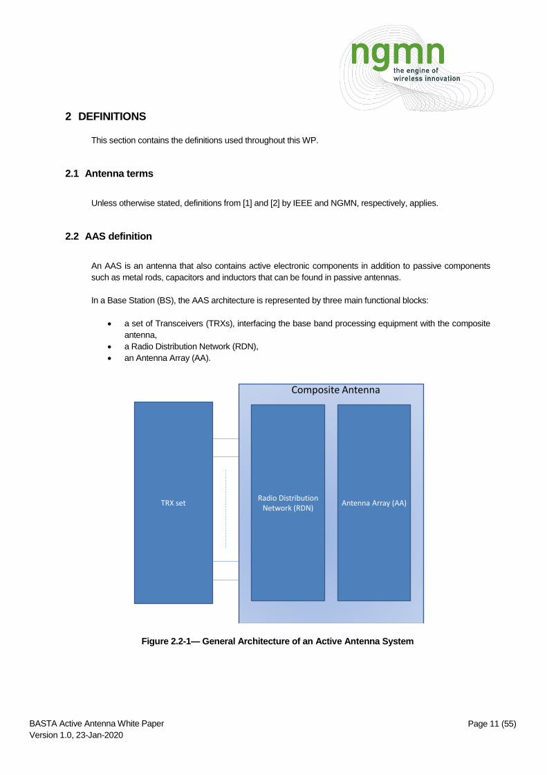
2.2 AAS definition
An AAS is an antenna that also contains active electronic components in addition to passive components
such as metal rods, capacitors and inductors that can be found in passive antennas.
In a Base Station (BS), the AAS architecture is represented by three main functional blocks:
a set of Transceivers (TRXs), interfacing the base band processing equipment with the composite
antenna,
a Radio Distribution Network (RDN),
an Antenna Array (AA).
TRX setRadio Distribution
Network (RDN)Antenna Array (AA)
Composite Antenna
Figure 2.2-1— General Architecture of an Active Antenna System

Page 12 (55) BASTA Active Antenna White Paper
Version 1.0, 23-Jan-2020
The TRX consists of transmitter units (TXUs) and receiver units (RXUs). The TXUs take the baseband signals
on input and provide RF signals on output. Such RF signals are distributed to the elements of the antenna
array via an RDN. An RXU performs the reverse of the TXU operations.
In 3GPP documents, for example in [4], 3 different BS types are considered:
Type 1-C is already addressed in [2] and will not be dealt with in the current document.
The 1-H type has connectors between the TRX set and the composite antenna.
The 1-O and 2-O are integrated antennas and hence have no such connectors available.
2.3 Antenna Reference Coordinate System
In this whitepaper the antenna reference coordinate system is identified by a right-handed set of three
orthogonal axes (��, ��, 𝑧) whose origin coincides with the center of an antenna’s FF radiation sphere, whose
spherical angles (, φ) are defined as in the figure below:
Figure 2.3-1—Antenna Reference Coordinate System.

Page 13 (55) BASTA Active Antenna White Paper
Version 1.0, 23-Jan-2020
Figure 2.3-2— Definition of the azimuth angle φ
Figure 2.3-3— Definition of elevation angle
Page 14 (55) BASTA Active Antenna White Paper
Version 1.0, 23-Jan-2020
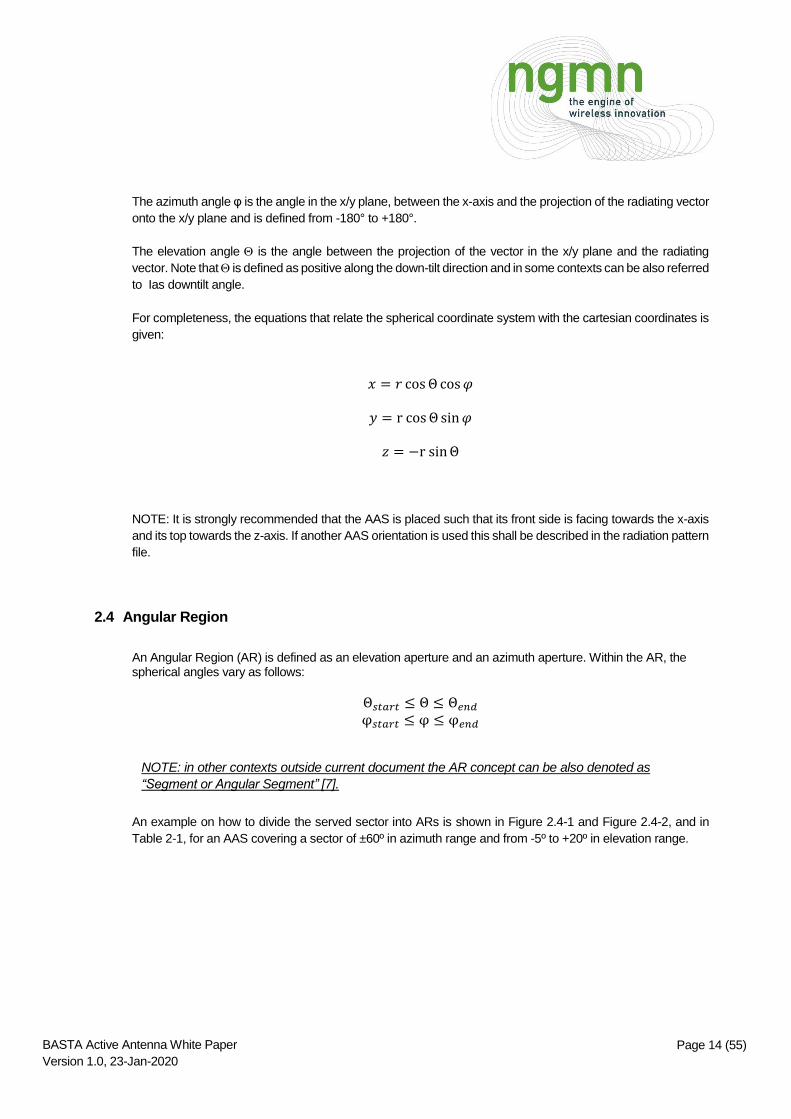
The azimuth angle φ is the angle in the x/y plane, between the x-axis and the projection of the radiating vector
onto the x/y plane and is defined from -180° to +180°.
The elevation angle is the angle between the projection of the vector in the x/y plane and the radiating
vector. Note that is defined as positive along the down-tilt direction and in some contexts can be also referred
to Ias downtilt angle.
For completeness, the equations that relate the spherical coordinate system with the cartesian coordinates is
given:
𝑥 = 𝑟 cosΘ cos𝜑
𝑦 = r cosΘ sin𝜑
𝑧 = −r sinΘ
NOTE: It is strongly recommended that the AAS is placed such that its front side is facing towards the x-axis
and its top towards the z-axis. If another AAS orientation is used this shall be described in the radiation pattern
file.
2.4 Angular Region
An Angular Region (AR) is defined as an elevation aperture and an azimuth aperture. Within the AR, the spherical angles vary as follows:
Θ𝑠𝑡𝑎𝑟𝑡 ≤ Θ ≤ Θ𝑒𝑛𝑑
φ𝑠𝑡𝑎𝑟𝑡 ≤ φ ≤ φ𝑒𝑛𝑑
NOTE: in other contexts outside current document the AR concept can be also denoted as
“Segment or Angular Segment” [7].
An example on how to divide the served sector into ARs is shown in Figure 2.4-1 and Figure 2.4-2, and in
Table 2-1, for an AAS covering a sector of ±60º in azimuth range and from -5º to +20º in elevation range.

Page 15 (55) BASTA Active Antenna White Paper
Version 1.0, 23-Jan-2020
Figure 2.4-1— Example of sector divided into ARs
Figure 2.4-2— Planar representation of the ARs

Page 16 (55) BASTA Active Antenna White Paper
Version 1.0, 23-Jan-2020
Angular
Region ID
Azimuth
Range
Elevation
Range
Angular
Region ID
Azimuth
Range
Elevation
Range
1 -60º to -45º
-5º to +0º
21 0º to +15º
5º to 10º 2 -45º to -30º 22 +15º to +30º
3 -30º to -15º 23 +30º to +45º
4 -15º to 0º 24 +45º to +60º
5 0º to +15º 25 -60º to -45º
10º to 15º
6 +15º to +30º 26 -45º to -30º
7 +30º to +45º 27 -30º to -15º
8 +45º to +60º 28 -15º to 0º
9 -60º to -45º
0º to 5º
29 0º to +15º
10 -45º to -30º 30 +15º to +30º
11 -30º to -15º 31 +30º to +45º
12 -15º to 0º 32 +45º to +60º
13 0º to +15º 33 -60º to -45º
15º to 20º
14 +15º to +30º 34 -45º to -30º
15 +30º to +45º 35 -30º to -15º
16 +45º to +60º 36 -15º to 0º
17 -60º to -45º
5º to 10º
37 0º to +15º
18 -45º to -30º 38 +15º to +30º
19 -30º to -15º 39 +30º to +45º
20 -15º to 0º 40 +45º to +60º
Table 2-1— AR tabular description of the example given in Figure 2.4-1
NOTE: In general, if irregular or more complex shapes of ARs are used, appropriate textual description and a
theta-phi plane drawing is required.
2.5 EIRP
Equivalent (or Effective) Isotropically Radiated Power (EIRP) in a direction, is the Total radiated power
radiated if the radiation intensity the device produces in that direction would be radiated isotropically. Hence,
EIRP is a farfield parameter like the radiation intensity. The SI unit of EIRP is W.
Radiation intensity [1] is the power radiated per unit solid angle and the SI unit is Watt per steradian (W/sr).
In formula,
𝐸𝐼𝑅𝑃(Θ, 𝜑) = 4𝜋𝐼(Θ, 𝜑)
where the solid angle of the full sphere (4𝜋 sr) is used.
Traditionally, EIRP is defined as the directive antenna gain (G) times the net power accepted by the antenna
(𝑃𝑎𝑐𝑐𝑒𝑝𝑡𝑒𝑑), see e.g. [1]. Moreover, gain is radiation intensity divided by the radiation intensity of an isotropic
radiator radiating the accepted power [1], i.e.,

Page 17 (55) BASTA Active Antenna White Paper
Version 1.0, 23-Jan-2020
𝐺(Θ, 𝜑) =𝐼(Θ, 𝜑)
𝑃𝑎𝑐𝑐𝑒𝑝𝑡𝑒𝑑/4𝜋
Note that the traditional definition also implies 𝐸𝐼𝑅𝑃(Θ, 𝜑) = 4𝜋𝐼(Θ, 𝜑). In this form the definition of EIRP has
the advantage of being independent of accepted power and gain which are not measureable for tightly
integrated AASs.
Moreover, the radiation intensity is related to the effective value of the electric field strength in the farfield
region as
𝐼(Θ, 𝜙) = lim 𝑟→∞
|�� (𝑟, Θ, 𝜑)|2
𝑍0
𝑟2
Here, 𝑍0 ≈ 377 Ω is the impedance of vaccuum. Hence, EIRP can be obtained by measuring the electric field
strength in a single point in the farfield region.
Relations to other parameters
EIRP = 𝑆(r, 𝜃, 𝜙)4𝜋𝑟2 where r is the distance from the antenna and 𝑆(𝑟, 𝜃, 𝜙) is the radial power flux
per unit area.
EIRP(𝜃, 𝜙) = 𝐷(𝜃, 𝜙)TRP where TRP is the Total radiated Power and D is directivity.
In general, it is not always possible to measure 𝑃𝑎𝑐𝑐𝑒𝑝𝑡𝑒𝑑 in integrated AAS products as there is not a connector
where the power can be measured. In such situations, the AAS Gain is introduced which can be derived as
the EIRP divided by the “configured output power” – which is the power that can be set on the O&M system.
NOTE: The meaning of “configured output power” is to be defined and provided by the manufacturer.
Attributes applied to EIRP, radiation intensity and related parameters follow [1] and are summarized here for
completeness:
Total denotes the sum (in linear scale) of two partial EIRP values corresponding to two orthogonal
polarizations of the electromagnetic field
Partial denotes a value corresponding to a specific polarization
Peak denotes the highest value with respect to angular directions.
If no attribute is used and no direction is specified, then “Peak Total” is intended.
Example: The statement “EIRP = 50 dBm”, means that the Peak Total EIRP is 50 dBm. An EIRP pattern is a
Total EIRP pattern if not otherwise stated. If only one polarization component is measured e.g. +45 degs
slanted polarization, then “Partial EIRP +45” should be used.
2.6 Beam
A beam is the radiation pattern of the antenna.
Beam might also be used as the main lobe of the radiation pattern of an antenna e.g. as stated in [2].
A beam can be characterised by:
Page 18 (55) BASTA Active Antenna White Paper
Version 1.0, 23-Jan-2020
The half-power beamwidth (HPBW) along two orthogonal directions, see definition of HPBW section
Fehler! Verweisquelle konnte nicht gefunden werden.
The beam peak direction: the direction of the maximum of the radiation pattern,
The beam peak centre: the direction corresponding to the center of the angular region where the HPBW
is calculated.
The radiation pattern ripple
In general, for symmetrical beams, the beam peak and the beam center are the same but in case of
asymetrical beams, or beams with strong ripple the beam peak and the beam centre directions might be
different, see example on Fehler! Verweisquelle konnte nicht gefunden werden.
An AAS is able to generate, at the same time, one or more beams with various time-dependent shapes
(different HPBW) and pointing to different directions using the same frequency band.
Even if it is not necessarily used in operational configurations, an AAS can generate, in any direction, for each
frequency, a particular beam, that is the most directive one among other possible beams sharing the same
direction. This beam is simply called the most directive beam.
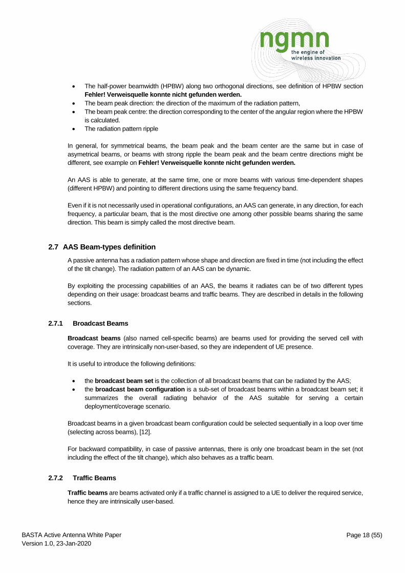
2.7 AAS Beam-types definition
A passive antenna has a radiation pattern whose shape and direction are fixed in time (not including the effect
of the tilt change). The radiation pattern of an AAS can be dynamic.
By exploiting the processing capabilities of an AAS, the beams it radiates can be of two different types
depending on their usage: broadcast beams and traffic beams. They are described in details in the following
sections.
2.7.1 Broadcast Beams
Broadcast beams (also named cell-specific beams) are beams used for providing the served cell with
coverage. They are intrinsically non-user-based, so they are independent of UE presence.
It is useful to introduce the following definitions:
the broadcast beam set is the collection of all broadcast beams that can be radiated by the AAS;
the broadcast beam configuration is a sub-set of broadcast beams within a broadcast beam set; it
summarizes the overall radiating behavior of the AAS suitable for serving a certain
deployment/coverage scenario.
Broadcast beams in a given broadcast beam configuration could be selected sequentially in a loop over time
(selecting across beams), [12].
For backward compatibility, in case of passive antennas, there is only one broadcast beam in the set (not
including the effect of the tilt change), which also behaves as a traffic beam.
2.7.2 Traffic Beams
Traffic beams are beams activated only if a traffic channel is assigned to a UE to deliver the required service,
hence they are intrinsically user-based.

Page 19 (55) BASTA Active Antenna White Paper
Version 1.0, 23-Jan-2020
It is useful to define two different traffic beam scenarios: Grid of Beams (GoB) and Eigen-Based Beamforming
(EBB).
2.7.2.1 Grid of Beams
In GoB configuration, traffic beams are selected among a finite number of pre-configured beams. An AAS
may have more than one GoB configuration in order to adapt to the cell scenario. An example of GoB
configuration is shown in Figure 2.7-1.
Figure 2.7-1: GoB example
2.7.2.2 Eigen-Based Beamforming
In Eigen-Based Beamforming (EBB), the calculation of the traffic beam (i.e. the array weights/precoders
applied to each Array Element) is done adaptively in real-time to cope with the variations of the propagation
channel. EBB relies on the reciprocity of the propagation channel.
2.8 Beamwidth
The X dB beamwidth is, in a radiation pattern cut containing the direction of the maximum of a lobe, the angle
between the two directions in which the radiation intensity is X dB below the maximum value.
When the beamwidth is not calculated over the Total radiated power radiation pattern (see section 2.8 in [2]),
the term co-polar beamwidth shall be used.
elevation
azimuth beam 1
beam 8 beam 7 beam 6 beam 5 beam 4 beam 3
beam 2
beam 9
beam 10 beam 11 beam 12

Page 20 (55) BASTA Active Antenna White Paper
Version 1.0, 23-Jan-2020
When X is equal to 3 dB, then the term half-power beamwidth (HPBW) is used.
In the Fehler! Verweisquelle konnte nicht gefunden werden. a peak normalized radiation pattern cut is d
epicted as a reference for azimuth and elevation half-power beamwidth calculation example. The distance
between the HPBW points (red) are used for HPBW calculations, and the mid-point (green) defines the beam
peak centre.
Figure 2.8-1— Illustration of HPBW beam peak centre, and beam peak direction.
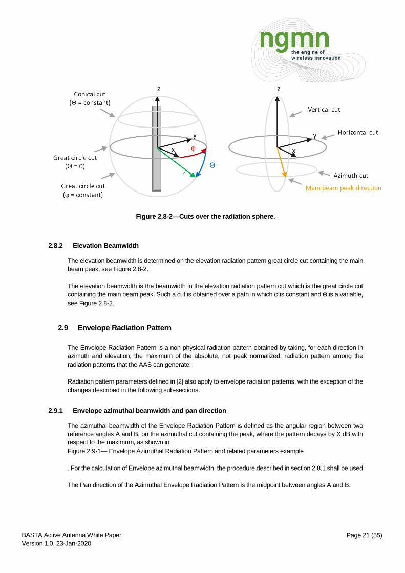
2.8.1 Azimuth Beamwidth
The azimuth beamwidth is determined on the azimuth radiation pattern conical cut containing the main beam
peak, see Figure 2.8-2
Page 21 (55) BASTA Active Antenna White Paper
Version 1.0, 23-Jan-2020
Figure 2.8-2—Cuts over the radiation sphere.
2.8.2 Elevation Beamwidth
The elevation beamwidth is determined on the elevation radiation pattern great circle cut containing the main
beam peak, see Figure 2.8-2.
The elevation beamwidth is the beamwidth in the elevation radiation pattern cut which is the great circle cut
containing the main beam peak. Such a cut is obtained over a path in which φ is constant and Θ is a variable,
see Figure 2.8-2.
2.9 Envelope Radiation Pattern
The Envelope Radiation Pattern is a non-physical radiation pattern obtained by taking, for each direction in
azimuth and elevation, the maximum of the absolute, not peak normalized, radiation pattern among the
radiation patterns that the AAS can generate.
Radiation pattern parameters defined in [2] also apply to envelope radiation patterns, with the exception of the
changes described in the following sub-sections.
2.9.1 Envelope azimuthal beamwidth and pan direction
The azimuthal beamwidth of the Envelope Radiation Pattern is defined as the angular region between two
reference angles A and B, on the azimuthal cut containing the peak, where the pattern decays by X dB with
respect to the maximum, as shown in
Figure 2.9-1— Envelope Azimuthal Radiation Pattern and related parameters example
. For the calculation of Envelope azimuthal beamwidth, the procedure described in section 2.8.1 shall be used
The Pan direction of the Azimuthal Envelope Radiation Pattern is the midpoint between angles A and B.

Page 22 (55) BASTA Active Antenna White Paper
Version 1.0, 23-Jan-2020
Figure 2.9-1— Envelope Azimuthal Radiation Pattern and related parameters example
The envelope azimuthal beamwidth is by default calculated with X equal to 3 (i.e. envelope azimuthal half-
power beamwidth) but other values may be chosen, e.g. X equal to 10 is typically used for coverage
calculation purposes.
2.9.2 Envelope elevation beamwidth and tilt direction
The elevation beamwidth of the Envelope Radiation Pattern is defined as the angular region between two
reference angles C and D, on the great circle cut containing the peak, where the pattern decays by X dB with
respect to the maximum, as shown in
Figure 2.9-2— Envelope elevation beamwidth and Tilt direction and related parameters example
.For the calculation of envelope elevation beamwidth, the procedure described in section 2.8.2 shall be used
The Tilt direction of the Elevation Envelope Radiation Pattern is the midpoint between angles C and D.

Page 23 (55) BASTA Active Antenna White Paper
Version 1.0, 23-Jan-2020
Figure 2.9-2— Envelope elevation beamwidth and Tilt direction and related parameters example
The envelope elevation beamwidth is by default calculated with X equal to 3 but other values may be chosen,
e.g. X equal to 10 is typically used for coverage calculation purposes.
2.9.3 Radiation pattern ripple
The radiation pattern ripple is defined as the difference between the highest and the lowest radiation pattern
levels per AR (see section 2.4) and it is expressed in dB. If no AR is defined, then it is intented as the azimuthal
and elevation scanning ranges, see Sections 3.2.10 and 3.2.11.

Page 24 (55) BASTA Active Antenna White Paper
Version 1.0, 23-Jan-2020
Figure 2.9-3— Ripple example of normalized envelope radiation pattern. The grey area illustrates the
AR.
2.10 Electrical Downtilt Angle
In addition to the beamforming capabilities of the AAS, that are achieved by modifying the feeding weights
(amplitude and phases) applied to each radiator or group of radiators connected to a TRX, the AAS might
have the additional capability to apply an offset in elevation to the whole set of patterns that the AAS can
generate, not due to a mechanical tilting of the antenna.
Unlike the feeding weights of each TRX that are adjusted dynamically during the normal operation of the AAS,
the electrical downtilt angle is intended to be a parameter that is set when the AAS is deployed and it is
modified only during network planning and optimization activities.
2.11 Radiation Pattern Format
Main elevation and azimuth cuts of the radiation pattern shall be given in MSI format.
If required, beam radiation patterns generated by the AAS are made available in 3D format, preferably via a
web link.
An example of the information required to exchange 3D patterns is listed below. In future releases of the WP,
a more formal format to exchange 3D patterns will be proposed.
The BASTA-AA reference coordinates are used
All units shall be declared (preferred choices are degrees for angles, dBm for EIRP and dBm for peak
values)
The file should contain:
o A file header with the necessary meta data: Peak EIRP, Configured output power, Power range,
Frequency (MHz) if single
o A data section with first two lines

Page 25 (55) BASTA Active Antenna White Paper
Version 1.0, 23-Jan-2020
%DATA
%POLARIZATION xxx
o And then column data with headers (frequency only if many): Theta (deg), Phi (deg), Frequency
(MHz), EIRP (dBm)
2.12 Frequency range and bandwidth
The following definitions are mainly taken from 3GPP terminology. See [3],[6],[4] for more details and additional
parameters.
2.12.1 Operating band and supported frequency range
The operating band defined here follows [4] for New Radio (NR) and [6] for Multi Standard Radio (MSR)
definition.
The supported frequency range is a specific band within the operating band and defined by a continuous
range between two frequencies.
2.12.2 Occupied bandwidth
The definition of Occupied Bandwidth (OBW) used e.g. in [4] and [6] applies. This refers to 99% symmetric power
utilization, i.e., 0.5% relative power leakage outside each band edge.
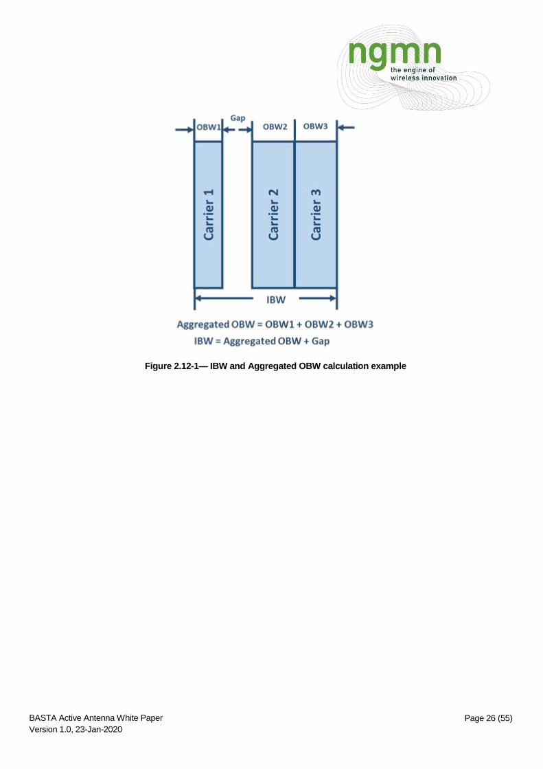
2.12.3 Aggregated Occupied Bandwidth
The Aggregated Occupied Bandwidth (Aggregated OBW), indicates the bandwidth occupied by multiple carriers
and is the sum of the OBWs of signals that can be output at the same time.
2.12.4 Instantaneous Bandwidth
The Instantaneous Bandwidth (IBW) is the span between the highest frequency and the lowest frequency of the
signals that can be output at the same time. The IBW is always greater or equal to the Aggregated OBW. IBW is
identical to “Maximum radiated Base Station RF Bandwidth for non-contiguous operation.” (D9.19) Sec. 4 in [5].
Figure 2.12-1 shows an example of calculation of IBW and Aggregated OBW.
Page 26 (55) BASTA Active Antenna White Paper
Version 1.0, 23-Jan-2020
Figure 2.12-1— IBW and Aggregated OBW calculation example

Page 27 (55) BASTA Active Antenna White Paper
Version 1.0, 23-Jan-2020
3 RF PARAMETERS AND SPECIFICATIONS
An AAS can be indicated as “BASTA-AAS compliant” only if:
Parameters used in its BASTA-AAS XML file or its BASTA-AAS datasheet coincide with the ones
listed in this section.
Values associated to each parameter used in its BASTA-AAS XML file or its BASTA-AAS datasheet
are calculated according to the methods defined here.
Its far-field radiation pattern files are made available.
3.1 Format, parameter definitions, validation and XML tags
Parameter description and format used in this WP follow what is provided in [2] section 3.1
For validation and specification of RF parameters, [2] will be used as a reference as well, and more specifically
the section 4 of it.
XML tags and examples are provided in a separate document that will be published together with the WP.
3.2 Required RF Parameters
3.2.1 Frequency range and bandwidth
Parameter Definition
Supported frequency band configuration(s), expressed in the terms defined in Section 2.12
Specification Definition
The frequency range(s) are specified in MHz.
If the AAS supports more than one Operating Band, the supported frequency range(s) shall be specified
for each Operating Band
Specification Example
Operating Band: n78
Supported Frequency Range: 3400-3600 MHz
Aggregated OBW: 160 MHz
IBW: 200 MHz
3.2.2 Number of carriers
Parameter Definition
Number of carriers supported by the AAS.

Page 28 (55) BASTA Active Antenna White Paper
Version 1.0, 23-Jan-2020
Specification Definition
For defining the number of carriers it is recommended to follow 3GPP documents [4] for New Radio
(NR) and [6] for Multi Standard Radio (MSR)
If the AAS supports more than one Operating Band, the supported number of carriers shall be
specified for each Operating Band
Specification Example
o Number of Carriers: 2
3.2.3 Polarization
Parameter Definition
The nominal polarization associated to the radiating elements of the AAS.
Specification Definition
Linear polarizations are declared as: H and V, +45 and -45, etc
Circular polarizations are typically declared as RHCP and LHCP.
Specification Example
Type: Polarization:
o +45º and -45º
3.2.4 Maximum Total Output RF power
Parameter Definition
The Maximum Total Output RF power is the maximum power achievable by the AAS during the transmitter
ON period, typically when all power amplifiers have the (same) maximum power at their outputs. Maximum
Total Output RF power is identical to “OTA BS Output Power” Sec 9.5 in [4], this is a TRP value declared
by the vendor.
Power values are intended to be RMS with respect to time.
Specification Definition
Maximum Total Output RF power is specified in W or dBm.
Specification Example
Type: Absolute
o Maximum RF power: 200 W

Page 29 (55) BASTA Active Antenna White Paper
Version 1.0, 23-Jan-2020
3.2.5 Broadcast Beam Set
Parameter Definition
A broadcast beam set is defined as the collection of all the preconfigured broadcast beams (see section 2.7.1).
Each beam is declared according to the table below. The configured output power associated to the given
EIRP shall be reported.
Specification Definition
Beam ID Frequency
Band
EIRP Azimuth Elevation
HPBW Pan HPBW Tilt
[dBm] [deg] [deg] [deg] [deg]
Specification Example
Beam ID Frequency
Band
EIRP Azimuth Elevation
HPBW Pan HPBW Tilt
[dBm] [deg] [deg] [deg] [deg]
1
n78
75.5
15
-52.5
6 6
2 76 -37.5
3 76.5 -22.5
4 77 -7.5
5 77 +7.5
6 76.5 +22.5
7 76 +37.5
8 75.5 +52.5
3.2.6 Broadcast Beam Configuration
Parameter Definition
A broadcast beam configuration is defined as the overall radiating behavior for a given deployment/coverage
scenario (see section 2.7.1) obtained by radiating one or more beams selected from the ones belonging to
the broadcast beam set.
The broadcast beam configuration can be:
Composed by just one of the beams of the broadcast beam set;
Composed by a number of broadcast beams of the broadcast beam set selected in a way for
solving specific coverage needs. There can be a different number of available broadcast beam
configuration implemented by the AAS, each one composed by beams belonging to the broadcast
beam set.
Sweeping across beams type, see section 2.7.1.
. The broadcast beam configuration can:
Have an associated envelope radiation pattern as described in section 2.9

Page 30 (55) BASTA Active Antenna White Paper
Version 1.0, 23-Jan-2020
Refer to a single beam ID. In the case this section is not relevant
Example of configuration:
A possible configuration may comprise 8 beams, with the same elevation pointing direction (θ = 0 degs for
example) and equally distributed in azimuth from – 50 to + 50 degs. The following picture illustrates this
example. Each single beam is depicted in green, the red curves (H65) correspond to a traditional coverage
beam of a passive antenna.
Figure 3.2-1— Broadcast beams configuration example (8 beams)
Other possible examples are depicted in the following pictures.

Page 31 (55) BASTA Active Antenna White Paper
Version 1.0, 23-Jan-2020
Elevation
Azimut
Elevation
Azimut
Configuration 1 (8 beams)
Configuration 2 (8 beams)
Figure 3.2-2—Broadcast beams configuration examples, using 8 beams where the green and orange
dots indicate the envelope centre and peak direction, respectively (see also Figure 2.8-1).
Specification Definition
For each configuration ID the main characteristics of the corresponding envelope radiation pattern
are to be provided according to the following table format. For the values of Pan, Tilt and
Beamwidth, either a single value or a set of values can be stated. If there is more than one beam,
by default we can assume that sweeping across beams is applied, see section 2.7.1.
Config.
ID
Frequency
Band
EIRP
Envelope Azimuth Envelope Elevation
HPBW Pan Conical Cut
Direction HPBW Tilt
Great Circle
Cut Direction
[dBm] [deg] [deg] [deg] [deg] [deg] [deg]
Specification Example
Config.
ID
Frequency
Band
EIRP
Envelope Azimuth Envelope Elevation
HPBW Pan Conical Cut
Direction HPBW Tilt
Great Circle
Cut Direction
[dBm] [deg] [deg] [deg] [deg] [deg] [deg]
1 n78
77 60 0 0,5,10 6 0,5,10 7.5
2 74 60 0 0,3,6 12 0,3,6 7.5
Page 32 (55) BASTA Active Antenna White Paper
Version 1.0, 23-Jan-2020
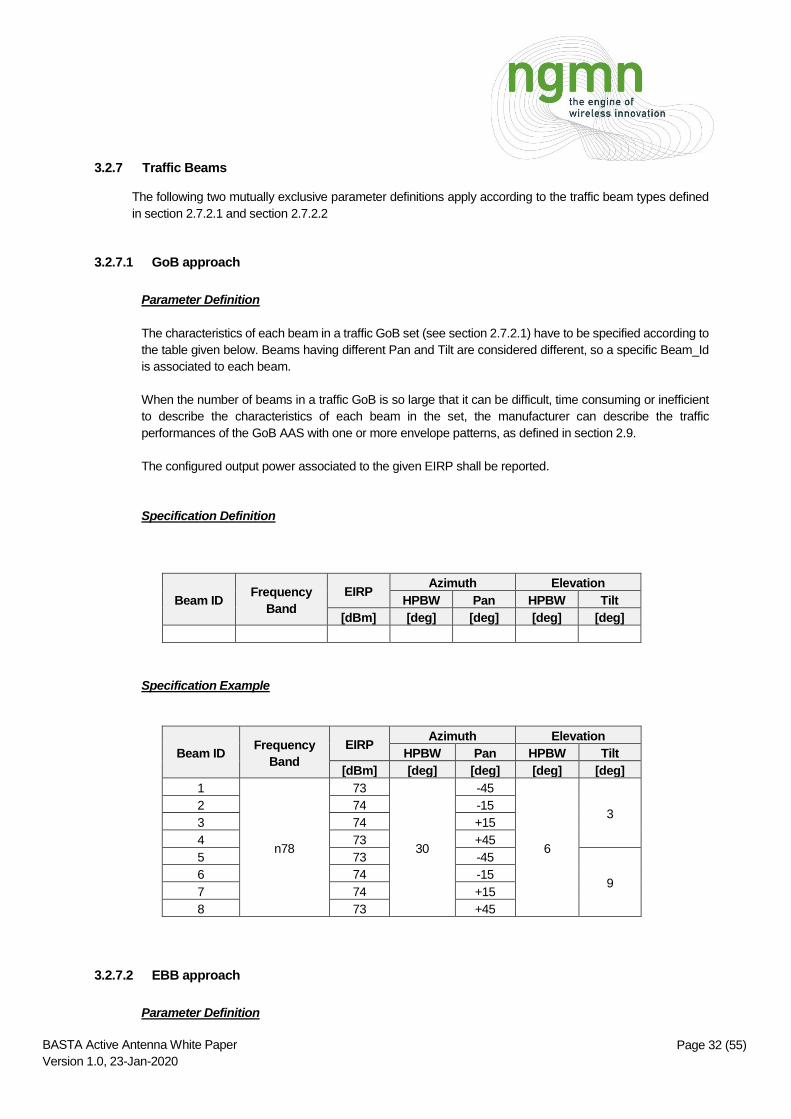
3.2.7 Traffic Beams
The following two mutually exclusive parameter definitions apply according to the traffic beam types defined
in section 2.7.2.1 and section 2.7.2.2
3.2.7.1 GoB approach
Parameter Definition
The characteristics of each beam in a traffic GoB set (see section 2.7.2.1) have to be specified according to
the table given below. Beams having different Pan and Tilt are considered different, so a specific Beam_Id
is associated to each beam.
When the number of beams in a traffic GoB is so large that it can be difficult, time consuming or inefficient
to describe the characteristics of each beam in the set, the manufacturer can describe the traffic
performances of the GoB AAS with one or more envelope patterns, as defined in section 2.9.
The configured output power associated to the given EIRP shall be reported.
Specification Definition
Beam ID Frequency
Band
EIRP Azimuth Elevation
HPBW Pan HPBW Tilt
[dBm] [deg] [deg] [deg] [deg]
Specification Example
Beam ID Frequency
Band
EIRP Azimuth Elevation
HPBW Pan HPBW Tilt
[dBm] [deg] [deg] [deg] [deg]
1
n78
73
30
-45
6
3 2 74 -15
3 74 +15
4 73 +45
5 73 -45
9 6 74 -15
7 74 +15
8 73 +45
3.2.7.2 EBB approach
Parameter Definition

Page 33 (55) BASTA Active Antenna White Paper
Version 1.0, 23-Jan-2020
An AAS implementing traffic beams by using the EBB approach generates, in real time, radiation patterns
whose shape depends on traffic conditions. For such systems, the radiating performance is summarized by
the envelope radiation pattern as defined in section 2.9.
The configured output power associated to the given EIRP shall be reported.
Specification Definition
The EBB envelope radiation pattern characteristics are described according to the following table:
Envelope
ID
Frequency
Band
EIRP Ripple Azimuth Elevation
HPBW Pan HPBW Tilt
[dBm] [dB] [deg] [deg] [deg] [deg]
The maximum EIRP and the associated envelope radiation pattern correspond to an unlikely situation in which
all the power is assigned to a single beam, to one user only, and in LoS (Line of Sight) conditions. However,
this situation is important in the context of EMF, since it gives the absolute maximum EIRP in a given direction.
NOTE: For EBB, as the number of patterns that can be generated is unlimited, the envelope radiation
pattern can be created by means of software taking as input the tested radiation pattern of each TRX,
the array factor and the pre-coders calculated for each direction.
Specification Example
Envelope
ID
Frequency
Band
EIRP Ripple Azimuth Elevation
HPBW Pan HPBW Tilt
[dBm] [dB] [deg] [deg] [deg] [deg]
1 n78 77 3 60 0 12 6
3.2.8 Minimum Azimuth HPBW
Parameter Definition
The minimum azimuth HPBW that can be achieved when all the radiators in the AAS are active and fed with
uniform phase and amplitude
Specification Definition
Range of values over frequency in degrees.
The HPBW is calculated from the Total radiated power radiation pattern.
Specification Example

Page 34 (55) BASTA Active Antenna White Paper
Version 1.0, 23-Jan-2020
Minimum Azimuth HPBW = 12° to 16°
3.2.9 Minimum Elevation HPBW
The minimum elevation HPBW that can be achieved when all the radiators in the AAS are active and fed
with uniform phase and amplitude
Specification Definition
Range of values over frequency in degrees.
The HPBW is calculated from the Total radiated power radiation pattern.
Specification Example
Minimum Elevation HPBW = 5.5° to 7.5°
3.2.10 Azimuth scanning range
Parameter Definition
Range of angles in azimuth in which the AAS is optimized and intended to be operated. It is a subset of the
OTA peak direction set defined in 3GPP, see [4] and [6]
Specification Definition
The nominal range of values in degrees.
Specification Example
Azimuth Scanning Range = –60° to +60°
3.2.11 Elevation scanning range
Parameter Definition
Angular range in elevation in which the AAS is optimized and intended to be operated. It is a subset of the
OTA peak direction set defined in 3GPP, see [5] and [13].
Specification Definition
The nominal range of values in degrees.
Specification Example
Page 35 (55) BASTA Active Antenna White Paper
Version 1.0, 23-Jan-2020
Elevation Scanning Range = –15° to +15°
3.2.12 Number of Tx/Rx channels
Parameter Definition
Number of independent TX and RX channels in the AAS. For each TX/RX branch there can be one or
more radiating elements connected to it.
Specification Definition
mTnR:, Where m is the number of TX and n is the number of RX
Specification Example
Number of Tx/Rx channels = 64T64R
3.2.13 Maximum number of layers
Parameter Definition
Maximum number of data streams sharing time and frequency resources that the AAS can handle
simultaneously. As an example, the layers can be associated to multiple users (MU-MIMO), one single
user (SU-MIMO) or a combination of both, i.e., multiple users having each of them one or multiple layers
associated.
Specification Definition
Integer value describing the maximum number of layers
Specification Example
Maximum number of layers = 8

Page 36 (55) BASTA Active Antenna White Paper
Version 1.0, 23-Jan-2020
4 MONITORING COUNTERS
In the context of RF-EMF exposure assessment [7] and [8], it is required that antenna manufacturers make
available to operators a certain number of counters (see Section B.6.5.3 in [7] and Section 13.3.3.3 in [8]). In
line with those requirements, the following power monitoring counters are defined:
Total radiated power counter
Directional power counters
The following characteristics mandatorily apply to such counters:
counters names and formats are declared by AAS manufacturers;
counters are made available to the operator’s Network Management System;
the averaging process is performed over a 6-minute time interval or its sub-multiple (e.g. 10 s, 30 s,
60 s, etc.), in line with what is specified in the applicable RF-EMF exposure regulations;
the time-averaging methodology is described (e.g. moving window…).
The availability of monitoring counters is required.
Specification Example
Total Radiated Power Counter: Available
Per AR Radiated Power Counter: Available
Per Beam Radiated Power Counter: NotAvailable
If radiation control mechanisms are implemented, see Section 5, the corresponding counters are required.
NOTE: Counter reporting time interval may not correspond to average time interval
4.1 Total radiated power counter
The counter that monitors the total radiated power over the full sphere shall report:
the time-averaged power level;
as an option, its Probability Distribution Function (PDF).
4.2 Directional power counters
Directional power counters are introduced to monitor the time-averaged power delivered to specific directions
where exposure issues can happen.
Directional power counters can be associated to either an AR (per-AR radiated power counter) or a specific
beam (per-beam radiated power counter).
Page 37 (55) BASTA Active Antenna White Paper
Version 1.0, 23-Jan-2020
Per-AR radiated power counter can be used for both GoB and EBB traffic beam implementation choices while
per-beam radiated power counter might be more straightforwardly applicable to GoB solutions. Anyway, it is
not necessary to have both types of counters implemented and it is up to the AAS’s manufacturer to decide
which type of counter is more suitable for its own AAS product.
4.2.1 Per-angular region radiated power counter
The power radiated through an AR (AR TRP) is defined as:
𝐴𝑅 𝑇𝑅𝑃 =1
4𝜋∫ ∫ EIRP(Θ, 𝜑)𝑐𝑜𝑠ΘdΘd𝜑
𝜑𝑚𝑎𝑥
𝜑𝑚𝑖𝑛
Θ𝑚𝑎𝑥
Θ𝑚𝑖𝑛
being Θmin, Θmax, φmin, φmax the limits of the AR.
The per-AR radiated power counter monitors the time-averaged power radiated through each AR the served
sector is divided into (AR definition and example is given in section 2.4).
Each AR needs to be described and identified with an ID, as specified in 2.4.
For each AR, the per-AR radiated power counter shall report:
the AR ID it is associated to;
the time-averaged power level;
and optionally, the Probability Distribution Function (PDF) of the monitored power levels.
Similar counter reporting EIRP can also be provided.
NOTE: The power reported in each AR is the whole power radiated by the AAS in that region.
4.2.2 Per-beam radiated power counter
The per-beam radiated power counter monitors the time-averaged power radiated by each beam in the beam
set the antenna is configured to use.
For each beam, the per-beam radiated power counter shall report:
the beam ID it is associated to;
the time-averaged power value;
and optionally, the Probability Distribution Function (PDF) of the monitored power levels.
Similar counter reporting EIRP can also be provided.

Page 38 (55) BASTA Active Antenna White Paper
Version 1.0, 23-Jan-2020
5 RADIATED POWER CONTROL MECHANISMS
In this chapter the capability of controlling the AAS radiated power [1], either statically or dynamically
depending on the scenario where it is operated, is addressed.
The purpose of such mechanisms is to limit the power radiated by an AAS, either in general or towards specific
directions (e.g. to comply with RF-EMF exposure limits).
Power limiting mechanisms are always associated to the corresponding power monitoring counters described
in chapter Fehler! Verweisquelle konnte nicht gefunden werden., which allow the operator to monitor the
evolution of the power radiated by the AAS over time.
The availability of radiated power control mechanisms is required.
Specification Example
Total Radiated Power Control: Available
Per AR Radiated Power Control: Available
Per Beam Radiated Power Control: NotAvailable
5.1 Total radiated power limiting mechanism
The total radiated power limiting mechanism indicates the capability to limit the Total radiated power radiated
by an AAS. Implementation-dependent options are to limit:
the peak power level;
the time-averaged power level.
If such mechanism is supported, whatever option is implemented, the vendor shall provide:
a description of the mechanism, by explicitly indicating whether the implemented mechanism is
either static or dynamic;
the range and the steps used to limit the power.
5.2 Directional radiated power limiting mechanism
The directional radiated power limiting mechanism indicates the capability to limit the power radiated by an
AAS towards specific directions. Implementation-dependent options are to limit:
the peak power level;
the time-averaged power level.
If such mechanism is supported, whatever option is implemented, the vendor shall provide:

Page 39 (55) BASTA Active Antenna White Paper
Version 1.0, 23-Jan-2020
a description of the mechanism, by explicitly indicating whether the implemented mechanism is
either static or dynamic;
the range and the steps used to limit the power per direction.
A direction can be defined either by the AR it refers to or by the beam associated to it in case of GoB
approach. Whatever choice is made, two different directional power limiting mechanisms can be defined
(associated to the corresponding directional power monitoring counters of sections 4.2.1 and 4.2.2), which
are described in the two following two sections.
5.2.1 Per-AR radiated power limiting mechanism
The per-AR radiated power limiting mechanism indicates the capability to limit the power radiated by an AAS
towards a specific AR. Implementation-dependent options are to limit:
the peak power level;
the time-averaged power level.
If such mechanism is supported, whatever option is implemented, the vendor shall provide:
the identification of the AR where the power limiting mechanism is operated;
a description of the mechanism, by explicitly indicating whether the implemented mechanism is either static or
dynamic;
the range and the steps used to limit the power per-AR.
5.2.2 Per-beam radiated power limiting mechanism
The per-beam radiated power limiting mechanism indicates the capability to limit the power of a specific
beam radiated by an AAS. Implementation-dependent options are to limit:
the peak power level;
the time-averaged power level.
If such mechanism is supported, whatever option is implemented, the vendor shall provide:
Beam ID (Section 3.2.7.1) where the power limiting mechanism is operated;
a description of the mechanism, by explicitly indicating whether the implemented mechanism is
either static or dynamic;
the range and the steps used to limit the power per beam.
Page 40 (55) BASTA Active Antenna White Paper
Version 1.0, 23-Jan-2020
6 MECHANICAL PARAMETERS AND SPECIFICATIONS
Unless otherwise stated, mechanical definitions and specifications in [2] are applicable. The required
parameters in [2] are:
Weight
Dimensions
Wind load
Max. operational wind speed (km/h)
Survival wind speed (km/h)
Required parameters that are not considered in [2] are listed below.
6.1 Heat dissipation
Parameter Definition
Maximum Heat Dissipation
Specification Definition
Nominal values in kilowatt
Specification Example
Maximum Heat Dissipation = 0.47kW
NOTE: The manufacturers may specify the cooling type e.g. natural cooling
6.2 Operational temperature
Parameter Definition
The operational temperature is the temperature range in which the AAS is designed to operate.
Specification Definition
Nominal values in Celsius degrees.
Minimum and Maximum operating temperatures.
Specification Example
Minimum temperature = -20°C; Maximum temperature = +60°C.
6.3 Relative humidity
Parameter Definition
The relative humidity is the relative humidity range in which the AAS is designed to operate.

Page 41 (55) BASTA Active Antenna White Paper
Version 1.0, 23-Jan-2020
Specification Definition
Nominal value in % RH.
Minimum and Maximum relative humidity values.
Specification Example
Minimum relative humidity = 5% RH; Maximum relative humidity = 100% RH
6.4 Ingress protection index
Parameter Definition
The ingress protection index is classification according to [11] in which the AAS is designed to operate.
Specification Definition
IP index
Specification Example
IP 65
6.5 Maximum power consumption
Parameter Definition
The maximum power consumption is the maximum power to be supported for operating the AAS
Specification Definition
Maximum Nominal values in Watt.
Specification Example
Maximum power consumption = 800W.
NOTE: The manufacturers may specify the maximum power consumptions conditions e.g. traffic load and
operating temperature (100% load 55 C).

Page 42 (55) BASTA Active Antenna White Paper
Version 1.0, 23-Jan-2020
APPENDIX A – EXAMPLE OF ACTIVE ANTENNA DATASHEET
NOTE: Below is an example of an active antenna datasheet. All the data in the table below is only
given for exemplary purposes and it is not intended to reflect the specifications of any existing
product.
RF parameters
Operating Band n78
Supported Frequency Range (MHz) 3400 - 3600
Aggregated OBW (MHz) 160
IBW (MHz) 200
Number of carriers Carriers:2, BW:100 MHz
Polarization +45° and –45°
Maximum total output RF power (W) 200, Absolute
Broadcast beam set See XML datasheet
Broadcast beam configuration See XML datasheet
Traffic beams – GoB approach See XML datasheet
Traffic beams – EBB approach See XML datasheet
Minimum azimuth HPBW (°) Min. 12, Max. 16
Minimum elevation HPBW (°) Min. 5.5, Max. 7.5
Azimuth scanning range (°) –60 to +60
Elevation scanning range (°) –15 to +15
TR/RX Channels TX: 64, RX: 64
Maximum number of layers 8
Monitoring counters
Total Radiated Power Counter Available
Per AR Radiated Power Counter Available
Per Beam Radiated Power Counter NotAvailable
Radiated power control mechanisms
Total Radiated Power Control Available
Per AR Radiated Power Control Available
Per Beam Radiated Power Control NotAvailable
Mechanical specifications
Dimensions (H x W x D) (mm) 1391 x 183 x 118
Weight Without Accessories (kg) 14.5
Weight of accessories only (kg) 3.4
Survival wind speed (km/h) 200
Windload – frontal at 150km/h (N) 500, at 150km/h
Windload – lateral at 150km/h (N) 360, at 150km/h
Heat Dissipation (kW) 0.47, Natural cooling
Operational Temperature (ºC) –20 to +60
Relative humidity 5% RH~100% RH
Ingress protection index IP65
Maximum power consumption (W) 800
Table A-1— AAS datasheet example

Page 43 (55) BASTA Active Antenna White Paper
Version 1.0, 23-Jan-2020
APPENDIX B – MIXED PASSIVE-ACTIVE ANTENNA SYSTEMS
Informative appendix on Mechanical Installation Kit (MIK) for mixed passive-active antenna systems. This
information is temporally maintained in the BASTA AA white paper, and the plan is to move it to a specific
white paper focusing on site solutions.
Generally, 5G antennas are deployed in the same sites as the legacy (2G/3G/4G) systems. To install this new
equipment, 3 possible options are shown in the figure below:
1. Add the new AAS antenna beside the existing antenna(s)
2. Create a modular “concept” to hide a M-MIMO antenna, thanks to a "Mechanical Installation Kit" (MIK)
3. Replacing the existing passive high band with an embedded MMIMO (interleaved solution)
Figure B-1— Deployment scenarios
Option 2 and 3 are mixed passive-active antenna systems. The scope of the present section is option 2 only.
Option 3 will be presented in a later version.
In many cases, option 1 is not possible or desirable (site negotiation, aesthetic reasons). In those cases, only
option 2 and 3 are possible. Option 2 is a “mixed passive-active” system, which is based on at least two
independent and field-replaceable units:
a) a Multi-Band passive antenna module called Passive Antenna System (PAS);
b) an enclosure called Mechanical Installation Kit (MIK) to host a M-MIMO AAS inside.
General description and parameters of the MIK solution
The MIK is developed to fit the dimensions of the PAS.

Page 44 (55) BASTA Active Antenna White Paper
Version 1.0, 23-Jan-2020
Mixed system
PAS
MIK
AAS
Figure B-2— Mixed passive-active antenna system
MIK mechanical parameters
The AAS should be capable of being installed afterwards inside the MIK by putting the MIK onto the ground
(without removing the pole brackets), installing the AAS inside and lifting the AAS+MIK back onto the
pole/mast into its original position.
As an example of implementation, the MIK (to host AAS) could be based of 3 main sub-units:
a) A rear mounting structure which allows to be installed on a pole/mast and to fix a Vendors's AAS on it
b) A radome covering the AAS and fixed on the mounting structure. This radome must have the same
shape and color as the radome of the PAS.
c) A disposable wind shield covering the back of the "empty" MIK. To be used with empty MIK and
removed when AAS is installed afterwards.
Note : the AAS is a field-installable unit and the MIK should allow easy AAS installation in the field at
ground level (installation on the pole/mast is not required).
An example of datasheet with the main MIK parameters is provided below. All environment parameter are
defined in passive antenna white paper [2]:
MIK parameters Example value Comment
The minimum dimensions (H x W x D) (mm) inside clearance (to host the AAS)
1000*450*250 MIK shall be aligned with the radome profile, width and depth of the PAS.
Weight of the "empty" MIK unit (kg) 10 Weight including brackets that are attached to the MAA??

Page 45 (55) BASTA Active Antenna White Paper
Version 1.0, 23-Jan-2020
Wind load (N) Frontal:500 Lateral:210
Rear side:515 at 150km/H
Max. operational wind speed (km/h) 150
Survival wind speed (km/h) 200
Temperature range (ºC) –40 to +55
Heat Dissipation Natural Cooling
Ingress protection index IP65
Relative humidity 5% RH~100% RH
Mounting/installation On a mast or pole of 55mm up
to 110mm diameter.
Mechanical tilt (degrees) 0-10
Should be available with 0 degrees mechanical tilt and 5 degrees mechanical tilt variants and should be interchangeable without the need of additional interfaces or tooling.
Table B-1— MIK datasheet example
Example of MIK performance validation
Even though the topic of AAS testing is not covered in this first release of the whitepaper, as a reference
relevant tests, for evaluation of the impact of the MIK on AAS, are described below.
The goal of the test is to evaluate the influence of the MIK on the AAS performance. For this purpose one UE
is emulated in different spatial directions. Pre-calculated pre-coders are then applied to the BBU to emulate
the UE different spatial directions. The AAS traffic beam patterns in the three steering directions specified in
Table B-2 below are generated and tested
Beams
Validation Scenario
Standalone AAS AAS with MIK
Azimuth :0° Elevation : 0°
Azimuth : 0° Elevation : Max
Azimuth : Max Elevation : 0°
Table B-2— List of traffic beams to be validated

Page 46 (55) BASTA Active Antenna White Paper
Version 1.0, 23-Jan-2020
For each of the tested beams, the parameters listed in Table B-3— List of the parameters to be calculated
and compared for each beam are calculated and compared. In addition, the azimuth and elevation radiation
pattern cuts shall be provided (see Figure 2.8-2 for the definition of the cuts) in order to allow the comparison
the patterns in terms of HPBW, SLS, etc.
The angles where the radiation pattern cuts are to be obtained shall correspond to the directions defined in
the Table B-2 above
Validation Scenario EIRP
(dBm) Azimuth Beam Peak
(°)
Elevation Beam Peak
(°)
Standalone AAS
AAS with MIK
Table B-3— List of the parameters to be calculated and compared for each beam
Page 47 (55) BASTA Active Antenna White Paper
Version 1.0, 23-Jan-2020
APPENDIX C – EMF SCENARIOS, ASSUMPTIONS AND EXAMPLES – INFORMATIVE
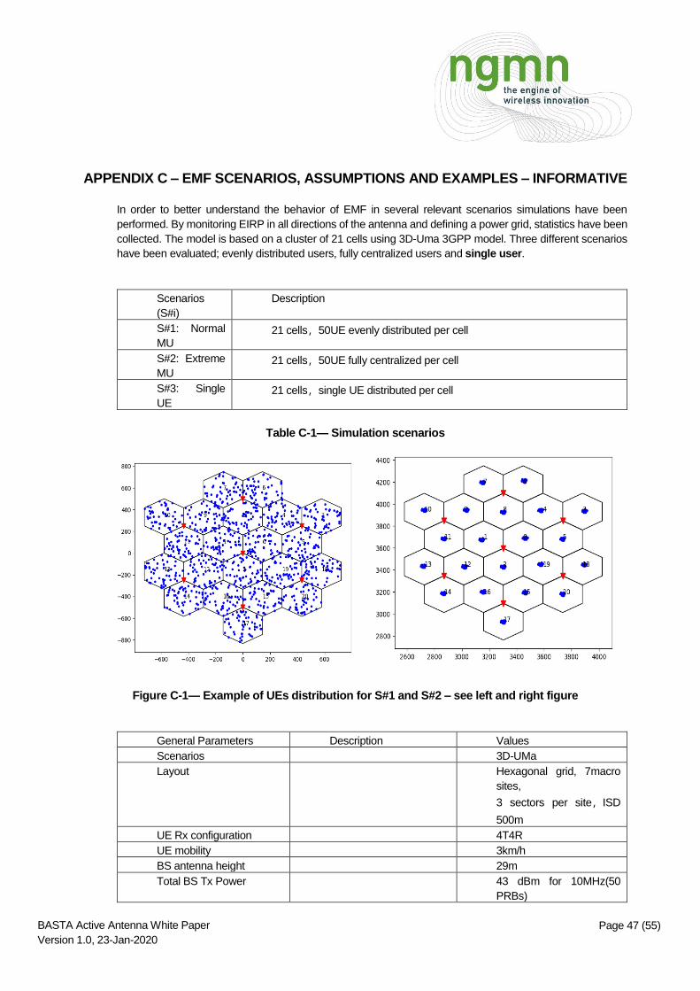
In order to better understand the behavior of EMF in several relevant scenarios simulations have been
performed. By monitoring EIRP in all directions of the antenna and defining a power grid, statistics have been
collected. The model is based on a cluster of 21 cells using 3D-Uma 3GPP model. Three different scenarios
have been evaluated; evenly distributed users, fully centralized users and single user.
Scenarios
(S#i)
Description
S#1: Normal
MU 21 cells,50UE evenly distributed per cell
S#2: Extreme
MU 21 cells,50UE fully centralized per cell
S#3: Single
UE 21 cells,single UE distributed per cell
Table C-1— Simulation scenarios
Figure C-1— Example of UEs distribution for S#1 and S#2 – see left and right figure
General Parameters Description Values
Scenarios 3D-UMa
Layout Hexagonal grid, 7macro
sites,
3 sectors per site,ISD
500m
UE Rx configuration 4T4R
UE mobility 3km/h
BS antenna height 29m
Total BS Tx Power 43 dBm for 10MHz(50
PRBs)
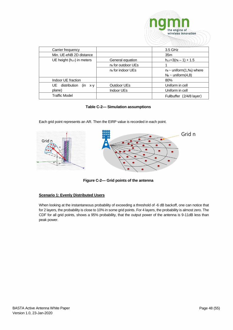
Page 48 (55) BASTA Active Antenna White Paper
Version 1.0, 23-Jan-2020
Carrier frequency 3.5 GHz
Min. UE-eNB 2D distance 35m
UE height (hUT) in meters General equation hUT=3(nfl – 1) + 1.5
nfl for outdoor UEs 1
nfl for indoor UEs nfl ~ uniform(1,Nfl) where
Nfl ~ uniform(4,8)
Indoor UE fraction 80%
UE distribution (in x-y
plane)
Outdoor UEs Uniform in cell
Indoor UEs Uniform in cell
Traffic Model Fullbuffer(2/4/8 layer)
Table C-2— Simulation assumptions
Each grid point represents an AR. Then the EIRP value is recorded in each point.
Figure C-2— Grid points of the antenna
Scenario 1: Evenly Distributed Users
When looking at the instantaneous probability of exceeding a threshold of -6 dB backoff, one can notice that
for 2 layers, the probability is close to 10% in some grid points. For 4 layers, the probability is almost zero. The
CDF for all grid points, shows a 95% probability, that the output power of the antenna is 9-11dB less than
peak power.

Page 49 (55) BASTA Active Antenna White Paper
Version 1.0, 23-Jan-2020
Figure C-3— Grids Power distribution (Scenario 1)
Figure C-4— Probability of exceeding the field strengt limit (2 layers, scenario 1)
0,00%
10,00%
20,00%
30,00%
40,00%
50,00%
60,00%
70,00%
80,00%
90,00%
100,00%
-40 -35 -30 -25 -20 -15 -10 -5 0
CD
F
Normalized Power(dB)
Grids Power Distribution @all grids
2layer 4layer 6layer 8layer
95%
-9-11
74
88
102
116
130
0,00%
2,00%
4,00%
6,00%
8,00%
10,00%
12,00%
26 34 42 50 58 66 74 82 90 98 106114122130138146154
V
Thet
a
H Phi
Probability of exceeding the field strength limit (2layer,3000TTI) instantaneously

Page 50 (55) BASTA Active Antenna White Paper
Version 1.0, 23-Jan-2020
Figure C-5— Probability of exceeding the field strength limit (4 layers, scenario 1)
If we now study the averaged power in each grid point, we find that the level is always less than the -6 dB
threshold (Pn=0.25). The averaging is here done over three seconds but similar result is expected using a
longer filtering time such as 6 minutes as defined by ICNIRP.
Figure C-6— Grid points for averaged power (scenario 1)
The conclusion is that thanks to multi paths, multi user and user distribution, it is clear that the average power
levels of a massive MIMO antenna system will be much lower than the peak levels.
Scenario 2: Centralized Users
74
88
102
116
130
0,00%
0,02%
0,04%
0,06%
0,08%
0,10%
0,12%
0,14%
0,16%
0,18%
0,20%
26
34
42
50
58
66
74
82
90
98
10
6
11
4
12
2
13
0
13
8
14
6
15
4
V
Thet
a
H Phi
Probability of exceeding the field strength limit (4layer,3000TTI) instantaneously

Page 51 (55) BASTA Active Antenna White Paper
Version 1.0, 23-Jan-2020
inthis scenario, all users are close to the antenna, we can see that the instantaneous probability that the power
level exceed the -6 dB threshold will be significantly higher.The CDF for all grid points, shows a 95%
probability, that the output power of the antenna is 8-10 dB less than peak power i.e. 1 dB more compared to
scenario 1.
Figure C-7— Grids Power distribution (Scenario 2)
0,00%
10,00%
20,00%
30,00%
40,00%
50,00%
60,00%
70,00%
80,00%
90,00%
100,00%
-40 -35 -30 -25 -20 -15 -10 -5 0
CD
F
Power(dB)
Grids Power Distribution @ all grids
2layer 4layer 6layer 8layer
95%
-8-10

Page 52 (55) BASTA Active Antenna White Paper
Version 1.0, 23-Jan-2020
Figure C-8— Probability of exceeding the field strength limit (2 layers, scenario 2)
Figure C-9— Probability of exceeding the field strength limit (4 layers, scenario 2)
If we now study the averaged power in each grid point, we find that the levels are very similar to those in
scenario 1, i.e. always less than the -6 dB threshold (Pn=0.25), see also [ref]. It is clear that beamforming can
create spatial separation between different users even though the users are close to each other.
74
88
102
116
130
0,00%
5,00%
10,00%
15,00%
20,00%
25,00%
30,00%
35,00%
40,00%
26
34
42
50
58
66
74
82
90
98
10
6
11
4
12
2
13
0
13
8
14
6
15
4
V
Thet
a
H Phi
Prob Exceeding Thr(2layer,3000TTI) instantaneously
74
88
102
116
130
0,00%
1,00%
2,00%
3,00%
4,00%
5,00%
6,00%
7,00%
26
34
42
50
58
66
74
82
90
98
10
6
11
4
12
2
13
0
13
8
14
6
15
4
V
Thet
a
H Phi
Prob Exceeding Thr(4layer,3000TTI) instantaneously
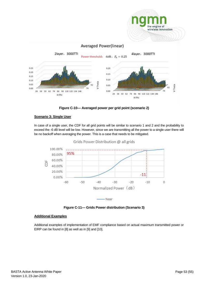
Page 53 (55) BASTA Active Antenna White Paper
Version 1.0, 23-Jan-2020
Figure C-10— Averaged power per grid point (scenario 2)
Scenario 3: Single User
In case of a single user, the CDF for all grid points will be similar to scenario 1 and 2 and the probability to
exceed the -6 dB level will be low. However, since we are transmitting all the power to a single user there will
be no backoff when averaging the power. This is a case that needs to be mitigated.
Figure C-11— Grids Power distribution (Scenario 3)
Additional Examples
Additional examples of implementation of EMF compliance based on actual maximum transmitted power or
EIRP can be found in [8] as well as in [9] and [10].
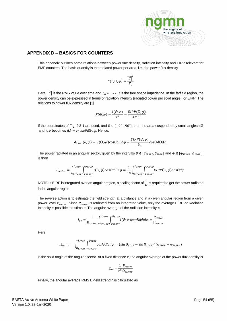
Page 54 (55) BASTA Active Antenna White Paper
Version 1.0, 23-Jan-2020
APPENDIX D – BASICS FOR COUNTERS
This appendix outlines some relations between power flux density, radiation intensity and EIRP relevant for
EMF counters. The basic quantity is the radiated power per area, i.e., the power flux density
𝑆(𝑟,Θ, 𝜑) =|𝐸 |
2
𝑍0
Here, |�� | is the RMS value over time and 𝑍0 ≈ 377 Ω is the free space impedance. In the farfield region, the
power density can be expressed in terms of radiation intensity (radiated power per solid angle) or EIRP. The
relations to power flux density are [1]
𝑆(Θ, 𝜑) =𝐼(Θ, 𝜑)
𝑟2=
𝐸𝐼𝑅𝑃(Θ, 𝜑)
4𝜋 𝑟2
If the coordinates of Fig. 2.3-1 are used, and Θ ∈ [−90∘, 90∘], then the area suspended by small angles dΘ
and d𝜑 becomes 𝑑𝐴 = 𝑟2𝑐𝑜𝑠𝜃dΘd𝜑. Hence,
d𝑃𝑟𝑎𝑑(𝜃, 𝜙) = 𝐼(Θ, 𝜑 )cosΘdΘd𝜑 =𝐸𝐼𝑅𝑃(Θ, 𝜑)
4𝜋𝑐𝑜𝑠ΘdΘd𝜑
The power radiated in an angular sector, given by the intervals 𝜃 ∈ [𝜃𝑆𝑇𝐴𝑅𝑇 , 𝜃𝑆𝑇𝑂𝑃] and 𝜙 ∈ [𝜙𝑆𝑇𝐴𝑅𝑇 , 𝜙𝑆𝑇𝑂𝑃 ],
is then
𝑃𝑠𝑒𝑐𝑡𝑜𝑟 = ∫ ∫ 𝐼(Θ, 𝜑)𝑐𝑜𝑠Θ𝑑Θ𝑑𝜑 =1
4𝜋∫ ∫ 𝐸𝐼𝑅𝑃(Θ, 𝜑)𝑐𝑜𝑠Θ𝑑𝜑
𝜑𝑆𝑇𝑂𝑃
𝜑𝑆𝑇𝐴𝑅𝑇
Θ𝑆𝑇𝑂𝑃
Θ𝑆𝑇𝐴𝑅𝑇
𝜑𝑆𝑇𝑂𝑃
𝜑𝑆𝑇𝐴𝑅𝑇
Θ𝑆𝑇𝑂𝑃
Θ𝑆𝑇𝐴𝑅𝑇
NOTE: If EIRP is integrated over an angular region, a scaling factor of 1
4𝜋 is required to get the power radiated
in the angular region.
The reverse action is to estimate the field strength at a distance and in a given angular region from a given
power level 𝑃𝑠𝑒𝑐𝑡𝑜𝑟. Since 𝑃𝑠𝑒𝑐𝑡𝑜𝑟 is retrieved from an integrated value, only the average EIRP or Radiation
Intensity is possible to estimate. The angular average of the radiation intensity is
𝐼𝑎𝑣 =1
Ω𝑠𝑒𝑐𝑡𝑜𝑟
∫ ∫ 𝐼(Θ, 𝜑)𝑐𝑜𝑠Θ𝑑Θ𝑑𝜑𝜑𝑆𝑇𝑂𝑃
𝜑𝑆𝑇𝐴𝑅𝑇
Θ𝑆𝑇𝑂𝑃
Θ𝑆𝑇𝐴𝑅𝑇
=𝑃𝑠𝑒𝑐𝑡𝑜𝑟
Ω𝑠𝑒𝑐𝑡𝑜𝑟
Here,
Ω𝑠𝑒𝑐𝑡𝑜𝑟 = ∫ ∫ 𝑐𝑜𝑠Θ𝑑Θ𝑑𝜑 = (sin Θ𝑆𝑇𝑂𝑃 − sin Θ𝑆𝑇𝐴𝑅𝑇)(𝜑𝑆𝑇𝑂𝑃 − 𝜑𝑆𝑇𝐴𝑅𝑇)𝜑𝑆𝑇𝑂𝑃
𝜑𝑆𝑇𝐴𝑅𝑇
Θ𝑆𝑇𝑂𝑃
Θ𝑆𝑇𝐴𝑅𝑇
is the solid angle of the angular sector. At a fixed distance 𝑟, the angular average of the power flux density is
𝑆𝑎𝑣 =1
𝑟2
𝑃𝑠𝑒𝑐𝑡𝑜𝑟
Ω𝑠𝑒𝑐𝑡𝑜𝑟
Finally, the angular average RMS E-field strength is calculated as
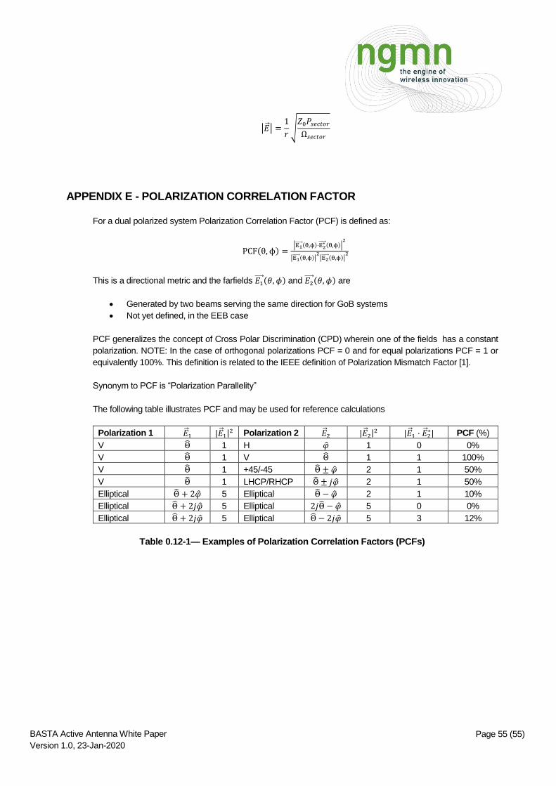
Page 55 (55) BASTA Active Antenna White Paper
Version 1.0, 23-Jan-2020
|�� | =1
𝑟√
𝑍0𝑃𝑠𝑒𝑐𝑡𝑜𝑟
Ω𝑠𝑒𝑐𝑡𝑜𝑟
APPENDIX E - POLARIZATION CORRELATION FACTOR
For a dual polarized system Polarization Correlation Factor (PCF) is defined as:
PCF(θ, ϕ) =|E1 (θ,ϕ)⋅E2
∗ (θ,ϕ)|2
|E1 (θ,ϕ)|2|E2 (θ,ϕ)|
2
This is a directional metric and the farfields 𝐸1 (𝜃, 𝜙) and 𝐸2
(𝜃, 𝜙) are
Generated by two beams serving the same direction for GoB systems
Not yet defined, in the EEB case
PCF generalizes the concept of Cross Polar Discrimination (CPD) wherein one of the fields has a constant
polarization. NOTE: In the case of orthogonal polarizations PCF = 0 and for equal polarizations PCF = 1 or
equivalently 100%. This definition is related to the IEEE definition of Polarization Mismatch Factor [1].
Synonym to PCF is “Polarization Parallelity”
The following table illustrates PCF and may be used for reference calculations
Polarization 1 �� 1 |�� 1|2 Polarization 2 �� 2 |�� 2|
2 |�� 1 ⋅ �� 2∗| PCF (%)
V Θ 1 H �� 1 0 0%
V Θ 1 V Θ 1 1 100%
V Θ 1 +45/-45 Θ ± �� 2 1 50%
V Θ 1 LHCP/RHCP Θ ± 𝑗�� 2 1 50%
Elliptical Θ + 2�� 5 Elliptical Θ − �� 2 1 10%
Elliptical Θ + 2𝑗�� 5 Elliptical 2𝑗Θ − �� 5 0 0%
Elliptical Θ + 2𝑗�� 5 Elliptical Θ − 2𝑗�� 5 3 12%
Table 0.12-1— Examples of Polarization Correlation Factors (PCFs)