new york state regents examination in...
TRANSCRIPT
New York State Regents Examination in Geometry
June 2010 Administration
Technical Report on Reliability and Validity
Technical Report Prepared for the New York State Education Department
by Pearson

Regents Examination Geometry
Copyright Developed and published under contract with the New York State Education Department by Pearson, 2510 North Dodge Street, Iowa City, IA, 52245. Copyright © 2010 by the New York State Education Department. Any part of this publication may not be reproduced or distributed in any form or by any means.
Page i
Table of Contents Introduction ...........................................................................................................1 Reliability ..............................................................................................................7
Internal Consistency..........................................................................................7 Standard Error of Measurement ........................................................................9 Classification Accuracy ...................................................................................13
Validity ................................................................................................................15 Content and Curricular Validity........................................................................15
Relation to Statewide Content Standards ....................................................15 Educator Input .............................................................................................16 Test Developer Input ...................................................................................16
Construct Validity ............................................................................................16 Item-Total Correlation ..................................................................................17 Rasch Fit Statistics ......................................................................................18 Correlation among Content Strands ............................................................21 Correlation among Item Types.....................................................................22 Principal Component Analysis .....................................................................22 Validity Evidence for Different Student Populations.....................................24
Equating, Scaling, and Scoring...........................................................................36 Equating Procedures.......................................................................................36 Scoring Tables..................................................................................................38 Pre-equating and Post-equating Contrast............................................................39
Scale Score Distribution......................................................................................43 Quality Assurance...............................................................................................54
Field Test ........................................................................................................54 Test Construction ............................................................................................55 Quality Control for Test Form Equating ...........................................................56
References .........................................................................................................57 Appendix A. Percentage of Students Included in Sample for Each Option .........58 Appendix B. Pre-equating and Post-equating Scoring Tables ............................60

Regents Examination Geometry
Page ii
List of Tables and Figures Table 1. Distribution of Needs/Resource Capacity (N/RC) Categories ................2 Table 2. Test Configuration by Item Type .............................................................2 Table 3. Test Blueprint by Content Strand ............................................................2 Table 4. Test Map by Standard and Content Strand.............................................3 Table 5. Raw Score Mean and Standard Deviation Summary..............................4 Table 6. Empirical Statistics for the Regents Examination in Geometry, June
2010 Administration ..............................................................................5 Table 7. Reliability Estimates for Total Test, MC Items Only, CR Items Only
and by Content Strands ........................................................................8 Table 8. Reliability Estimates and SEM for Total Population and
Subpopulations ...................................................................................11 Table 9. Raw-to-Scale-Score Conversion Table and Conditional SEM for the
Regents Examination in Geometry .....................................................12 Table 10. Classification Accuracy Table. ............................................................14 Table 11. Rasch Fit Statistics for All Items on Test.............................................20 Table 12. Correlation among Content Strands....................................................21 Table 13. Correlation among Item Types and Total Test ....................................22 Table 14. Factors and Their Eigenvalues ...........................................................23 Table 15. DIF Statistics for the Regents Examination in Geometry, Focal
Group: Female; Reference Group: Male.............................................28 Table 16. DIF Statistics for Regents Examination in Geometry, Focal Group:
Hispanic; Reference Group: White .....................................................30 Table 17. DIF Statistics for Regents Examination in Geometry, Focal Group:
African American; Reference Group: White ........................................32 Table 18. DIF Statistics for Regents Examination in Geometry, Focal Group:
High Need; Reference Group: Low Need ...........................................34 Table 19. Contrasts between Pre-equated and Post-operational Item
Parameter Estimates ..........................................................................40 Table 20. Comparisons of Raw Score Cuts and Percentages of Students in
Each of the Achievement Levels between Pre-equating and Post-equating Models .................................................................................42
Table 21. Scale Score Distribution for All Students.............................................43 Table 22. Scale Score Distribution for Male Students.........................................44 Table 23. Scale Score Distribution for Female Students.....................................45 Table 24. Scale Score Distribution for White Students .......................................46 Table 25. Scale Score Distribution for Hispanic Students...................................47 Table 26. Scale Score Distribution for African American Students .....................48 Table 27. Scale Score Distribution for English Language Learners ....................49 Table 28. Scale Score Distribution for Students with Low Socio-Economic
Status..................................................................................................50 Table 29. Scale Score Distribution for Students with Disabilities ........................51 Table 30. Descriptive Statistics on Scale Scores for Various Student Groups....52 Table 31. Performance Classification for Various Student Groups .....................53

Regents Examination Geometry
Page iii
List of Tables and Figures, Continued Table A 1. Percentage of Students Included in Sample for Each Option (MC
Only)..................................................................................................58 Table A 2. Percentage of Students Included in Sample at Each Possible
Score Credit (CR only) ......................................................................59 Table B 1. Comparison of Pre-equating and Post-equating Scoring Tables. ......60 Figure 1. Scree Plot for Principal Component Analysis of Items on the
Regents Examination in Geometry.......................................................24 Figure 2. Comparison of Relationship between Raw Score and Ability
Estimates between Pre-equating Model and Post-equating Model. .....41

Page 1
Introduction
In March 2005, the Board of Regents adopted a new Learning Standard for Mathematics and issued a revised Mathematics Core Curriculum, resulting in the need for the development and phasing in of three new mathematics Regents examinations: Integrated Algebra, Geometry, and Algebra 2/Trigonometry. These new Regents examinations in mathematics will replace the Regents Examinations in Mathematics A and Mathematics B. To fulfill the mathematics Regents examination requirement for graduation, students must pass any one of these new commencement-level Regents examinations. The first administration of the Regents Examination in Integrated Algebra took place in June 2008. The first administration of the Regents Examination in Geometry took place in June 2009. The first administration of the Regents Examination in Algebra 2/Trigonometry took place in June 2010.
The Regents Examination in Geometry is based on the content contained in the Mathematics Core Curriculum (Revised 2005). The first administration took place in June 2009 and the new standards were set. The same standards have been maintained through the use of equating for the subsequent administrations: August 2009, January 2010, and June 2010. In June 2010, a score collection effort was conducted, where a representative sample of students were identified across New York State and their answer sheets were sent back to Pearson for processing. Through the data collected, further reliability and validity evidence can be examined. This technical document provides such details based on the data collected from the June 2010 administration of the Regents Examination in Geometry.
First, discussions on reliability are presented, including classical test theory based reliability evidence, the Item Response Theory (IRT) based reliability evidence, evidence related to subpopulations, and reliability evidence on classification accuracy for three achievement levels. Next, validity evidence is described, including evidence in internal structure validity, content validity, and construct validity. Equating, scaling, and scoring approaches used for the Regents Examination in Geometry are then described. Contrasts between the pre-equating and the post-equating analyses are presented. Finally, scale score distributions for the entire state and for subpopulations are presented.
The analysis was based on data collected after the June 2010 administration. This technical report includes reliability and validity evidence for the tests, as well as summary statistics for the administration. The table below describes the distribution of public schools (Needs/Resource Capacity (N/RC) categories) and nonpublic schools. Based on the distribution, the sample resembles the characteristics of the population data collected from the June 2009 administration and can be considered representative. All the analysis in this report, therefore, is based on this representative data.

Regents Examination Geometry
Page 2
Table 1. Distribution of Needs/Resource Capacity (N/RC) Categories
Need/Resource Capacity Index
Number of Schools
Number of Students Percent
New York City 34 5,095 26.72
Large Cities 12 856 4.49
Urban-Suburban High Needs/Resource Capacity Index 8 1,019 5.34
Rural 25 1,060 5.56
Average Needs/Resource Capacity Index Districts 42 5,688 29.83
Low Needs/Resource Capacity Index Districts 20 3,390 17.78
Charter Schools 5 230 1.21
Non-Public Schools 27 1,731 9.08 Total 173 19,069
Table 2. Test Configuration by Item Type
Item Type Number of
Items Number of
Credits Percent of
Credits Multiple-Choice 28 56 65.12
Constructed-Response 10 30 34.88
Total 38 86 Table 3. Test Blueprint by Content Strand
Content Strands Number of Items
Number of Credits
2010 Percent of Credits
Target Percent of Credits
Geometric Relationships 4 8 9.30 8–12%
Constructions 2 4 4.65 3–7%
Locus 2 4 4.65 4–8% Informal and Formal
Proofs 17 38 44.19 41–47%
Transformational Geometry 4 10 11.63 8–13%
Coordinate Geometry 9 22 25.58 23–28%

Regents Examination Geometry
Page 3
Table 4. Test Map by Standard and Content Strand
Test Part
Item Number Item Type
Maximum Credit Content Strand
I 1 Multiple-Choice 2 Informal and Formal Proofs I 2 Multiple-Choice 2 Geometric Relationships I 3 Multiple-Choice 2 Informal and Formal Proofs I 4 Multiple-Choice 2 Coordinate Geometry I 5 Multiple-Choice 2 Constructions I 6 Multiple-Choice 2 Informal and Formal Proofs I 7 Multiple-Choice 2 Informal and Formal Proofs I 8 Multiple-Choice 2 Geometric Relationships I 9 Multiple-Choice 2 Coordinate Geometry I 10 Multiple-Choice 2 Coordinate Geometry I 11 Multiple-Choice 2 Informal and Formal Proofs I 12 Multiple-Choice 2 Informal and Formal Proofs I 13 Multiple-Choice 2 Coordinate Geometry I 14 Multiple-Choice 2 Coordinate Geometry I 15 Multiple-Choice 2 Transformational Geometry I 16 Multiple-Choice 2 Informal and Formal Proofs I 17 Multiple-Choice 2 Informal and Formal Proofs I 18 Multiple-Choice 2 Informal and Formal Proofs I 19 Multiple-Choice 2 Coordinate Geometry I 20 Multiple-Choice 2 Geometric Relationships I 21 Multiple-Choice 2 Transformational Geometry I 22 Multiple-Choice 2 Informal and Formal Proofs I 23 Multiple-Choice 2 Transformational Geometry I 24 Multiple-Choice 2 Coordinate Geometry I 25 Multiple-Choice 2 Informal and Formal Proofs I 26 Multiple-Choice 2 Informal and Formal Proofs I 27 Multiple-Choice 2 Informal and Formal Proofs I 28 Multiple-Choice 2 Locus II 29 Constructed-Response 2 Informal and Formal Proofs II 30 Constructed-Response 2 Geometric Relationships II 31 Constructed-Response 2 Informal and Formal Proofs II 32 Constructed-Response 2 Constructions II 33 Constructed-Response 2 Locus II 34 Constructed-Response 2 Coordinate Geometry III 35 Constructed-Response 4 Informal and Formal Proofs III 36 Constructed-Response 4 Transformational Geometry III 37 Constructed-Response 4 Informal and Formal Proofs IV 38 Constructed-Response 6 Coordinate Geometry
The scale scores range from 0 to 100 for all Regents examinations. The three achievement levels on the exams are Level 1 with a scale score from 0 to 64,

Regents Examination Geometry
Page 4
Level 2 with a scale score from 65 to 84, and Level 3 with a scale score from 85 to 100.
The Regents examinations consist of some number of multiple-choice (MC) items, and some number of constructed-response (CR) items. Table 2 shows how many MC and CR items there were on the Regents Examination in Geometry, as well as the number and percentage of credits for both item types. Table 3 reports item information by content strand. All items on the Regents Examination in Geometry were classified based on the mathematical standard.
Each form of the examination must adhere to strict rules indicating how many items per standard and content strand should be placed on a single form. In this way, the examinations can claim to measure the same concepts and standards from administration to administration, as long as the standards remain constant. Table 4 provides detailed classification of items in terms of content strand.
There are 28 MC items, each worth 2 credits, and ten CR items, worth from 2 to 6 credits each. Table 5 presents a summary of raw score means for the total number of MC items, the total number of CR items, and all questions combined. The standard deviation is also reported. Table 5. Raw Score Mean and Standard Deviation Summary
Item Type Raw Score Mean Standard Deviation
Multiple-Choice 36.66 9.89
Constructed-Response 17.93 8.53
Total 54.59 17.51
Table 6 reports the empirical statistics per item. The table includes item position on the test, item type, maximum item score value, content strand, the number of students included in the data who responded to the point biserial, item mean, and weighted item mean.

Regents Examination Geometry
Page 5
Table 6. Empirical Statistics for the Regents Examination in Geometry, June 2010 Administration
Item Position
Item Type
Max. Item
Score Content Strand
Number of
Students Point
Biserial Item Mean
Weighted Item Mean
1 Multiple-Choice 2 4 19,057 0.28 1.91 0.96 2 Multiple-Choice 2 1 19,062 0.29 1.90 0.95 3 Multiple-Choice 2 4 19,058 0.33 1.77 0.89 4 Multiple-Choice 2 6 19,060 0.37 1.75 0.87 5 Multiple-Choice 2 2 19,060 0.36 1.72 0.86 6 Multiple-Choice 2 4 19,057 0.33 1.68 0.84 7 Multiple-Choice 2 4 19,052 0.44 1.49 0.74 8 Multiple-Choice 2 1 19,051 0.36 1.38 0.69 9 Multiple-Choice 2 6 19,059 0.29 1.55 0.78
10 Multiple-Choice 2 6 19,052 0.49 1.47 0.74 11 Multiple-Choice 2 4 19,057 0.26 1.48 0.74 12 Multiple-Choice 2 4 19,058 0.36 1.50 0.75 13 Multiple-Choice 2 6 19,050 0.38 1.00 0.50 14 Multiple-Choice 2 6 19,052 0.50 1.44 0.72 15 Multiple-Choice 2 5 19,056 0.23 1.08 0.54 16 Multiple-Choice 2 4 19,000 0.38 1.11 0.55 17 Multiple-Choice 2 4 19,046 0.32 1.20 0.60 18 Multiple-Choice 2 4 19,058 0.41 1.31 0.65 19 Multiple-Choice 2 6 19,050 0.45 1.30 0.65 20 Multiple-Choice 2 1 19,044 0.21 0.96 0.48 21 Multiple-Choice 2 5 19,036 0.52 1.30 0.65 22 Multiple-Choice 2 4 19,062 0.49 1.57 0.79 23 Multiple-Choice 2 5 19,048 0.17 0.78 0.39 24 Multiple-Choice 2 6 19,019 0.24 0.95 0.47 25 Multiple-Choice 2 4 19,052 0.19 0.84 0.42 26 Multiple-Choice 2 4 19,046 0.26 0.79 0.40 27 Multiple-Choice 2 4 19,043 0.41 0.82 0.41 28 Multiple-Choice 2 3 19,044 0.36 0.64 0.32
29 Constructed-response 2 4 19,069 0.50 1.56 0.78
30 Constructed-response 2 1 19,069 0.49 1.55 0.77
31 Constructed-response 2 4 19,069 0.62 1.35 0.67
32 Constructed-response 2 2 19,069 0.58 1.20 0.60
33 Constructed-response 2 3 19,069 0.65 1.22 0.61
34 Constructed-response 2 6 19,069 0.56 1.50 0.75
35 Constructed-response 4 4 19,069 0.67 2.41 0.60
36 Constructed-response 4 5 19,069 0.69 2.32 0.58
37 Constructed-response 4 4 19,069 0.71 1.73 0.43
38 Constructed-response 6 6 19,069 0.70 3.10 0.52

Regents Examination Geometry
Page 6
The item mean score is a measure of the item difficulty, ranging from 0 to the item maximum score. The higher the item mean score relative to the maximum score attainable, the easier the item is. The following formula is used to calculate this index for both MC and CR items:
i i iM c / n= , where
iM = the mean score for item i ,
i c = the total credits students obtained on item i , and
in = the total number of students who responded to item i .
The weighted item mean score is the item mean score divided by the max item score, ranging from 0 to 1. The point biserial coefficient is a measure of the relationship between a student’s performance on the given item (correct or incorrect for MC items and raw score points for CR items) and the student’s score on the overall test. Conceptually, if an item has a high point biserial (i.e., 0.30 or above), it indicates that students who performed well on the test also performed relatively well on the given item and students who performed poorly on the test also performed relatively poorly on the given item. If the point biserial value is high, it is typically stated that the item did a good job discriminating between high performing and low performing students. Assuming the total test score represents the extent to which a student possesses the construct being measured by the test, high item total correlations indicate the items on the test require this construct to be answered correctly if it is an MC item, or a relatively high score out of the maximum credits possible if it is a CR item. The point biserial correlation coefficient was computed between the item score and the total score on the test with the target item score excluded (also called corrected point biserial correlation coefficient).
The possible range of the point biserial coefficient is − 1.0 to 1.0. In general, relatively high point biserials are desirable. A negative point biserial suggests that overall the most proficient students are getting the item wrong (if it is an MC item) or scoring low on the item (if it is a CR item) and the least proficient students are getting the item correct or scoring high. Any item with a point biserial that is near zero or negative should be carefully reviewed.
On the basis of the values reported in Table 6, the item means ranged from 0.64 to 3.1, while the maximum credits ranged from 2 to 6 for the 38 items on the test. The point biserial correlations were reasonably high, ranging from 0.17 to 0.71, suggesting good discriminative power on the items to differentiate students who scored high on the test from students who scored low on the test. Altogether, there were 10 items that had point biserial correlations lower than 0.30. In Appendix A, Tables A1 and A2 report the percentage of students at each of the possible score points for all items.

Regents Examination Geometry
Page 7
Reliability
Internal Consistency
Reliability is the consistency of the results obtained from a measurement. The focus of reliability should be on the results obtained from a measurement and the extent to which they remain consistent over time or among items or subtests that constitute the test. The ability to consistently measure students’ performance is a necessary prerequisite to making appropriate score interpretations.
As stated above, test score reliability refers to the consistency of the results of a measurement. This consistency can be seen in the degree of agreement between two measures on two occasions, or it can be viewed as the degree of agreement between the components and the overall measurement. Operationally, such comparisons are the essence of mathematically defined reliability indices.
All measures consist of an accurate, or true, score component and an inaccurate, or error, score component. Errors occur as a natural part of the measurement process and can never be entirely eliminated. For example, uncontrollable factors, such as differences in the physical world and changes in examinee disposition, may work to increase error and decrease reliability. This is the fundamental premise of classical reliability analysis and classical measurement theory. Stated explicitly, this relationship can be represented with the following equation:
Observed Score True Score Error Score= + . To facilitate a mathematical definition of reliability, these components can be rearranged to form the following ratio:
2 2
2 2 2True Score True Score
Observed Score True Score Error Score
Reliabilityσ σ
σ σ σ= =
+.
When there is no error, the reliability is the true score variance divided by true score variance, which is unity. However, as more error influences the measure, the error component in the denominator of the ratio increases. As a result, the reliability decreases.
Coefficient alpha (Cronbach, 1951), one of these internal consistency reliability indices, is provided for the entire test, for MC items only, for CR items only, for each of the content strands on the test, and for gender and ethnicity groups. Coefficient alpha is a more general version of the common Kuder-Richardson reliability coefficient and can accommodate both dichotomous and polytomous items. The formula for coefficient alpha is

Regents Examination Geometry
Page 8
( )
( )
2
211
i
x
SDkk SD
α⎛ ⎞⎛ ⎞= −⎜ ⎟⎜ ⎟⎜ ⎟−⎝ ⎠⎝ ⎠
∑ ,
where k = the number of items,
iSD = the standard deviation of the set of scores associated with item i , and
xSD = the standard deviation of the set of total scores.
Table 7. Reliability Estimates for Total Test, MC Items Only, CR Items Only and by Content Strands
Number of Items
Raw Score Mean
Standard Deviation Reliability1
Total Test 38 54.59 17.51 0.90
MC Items Only 28 36.66 9.89 0.81
CR Items Only 10 17.93 8.53 0.86
Geometric Relationships 4 5.78 1.86 0.33
Constructions 2 2.92 1.18 0.40
Locus 2 1.86 1.38 0.38
Informal and Formal Proofs 17 24.49 7.89 0.79
Transformational Geometry 4 5.47 2.87 0.42
Coordinate Geometry 9 14.06 5.39 0.68
Table 7 reports reliability estimates for the entire test, for MC items only, for CR items only, and by content strands measured by the test. Notably, the reliability estimate is a statistic, and, like all other statistics, it is affected by the number of items, or test length. When the reliability estimate is calculated for content strands, sometimes there can be as few as two items within a given content strand, and so it is unlikely the alpha coefficient will be high. On the basis of the Spearman-Brown formula (Feldt & Brennan, 1988), with all other things being equal, the longer the test or the greater the number of items, the higher the
1 When the number of items is small, the calculated reliability tends to be low, because as a statistic, reliability is sample size sensitive.

Regents Examination Geometry
Page 9
reliability coefficient estimate is likely to be. Intuitively, the more items the students are tested on, the more information can be collected and the more reliable the achievement measure tends to be. The reliability coefficient estimates for the entire test, MC items only, and CR items only were all reasonably high. Because the number of items per content strand tends to be small, the reliability coefficient for content strands tended not to be as high, especially for content strands Constructions and Locus (including only 2 items) and content strands Geometric Relationships and Transformational Geometry (including only 4 items).
Standard Error of Measurement
The standard error of measurement (SEM) uses the information from the test along with an estimate of reliability to make statements about the degree to which error is influencing individual scores. The SEM is based on the premise that underlying traits, such as academic achievement, cannot be measured exactly without a precise measuring instrument. The standard error expresses unreliability in terms of the reported score metric. The two kinds of standard errors of measurement are the SEM for the overall test and the SEM for individual scores. The second kind of SEM is sometimes called Conditional Standard Error of Measurement (CSEM). Through the use of CSEM, an error band can be placed around an individual score, indicating the degree to which error might have an impact on that score. The total test SEM is calculated using the following formula:
'1x XXSEM σ ρ= − , where
xσ = the standard deviation of the total test (standard deviation of the raw scores), and
'xxρ = the reliability estimate of the total test scores. Through the use of an Item Response Theory (IRT) model, CSEM can be computed with the information function. The information function for the number correct score x is defined as
' 2( )( , ) ii
i ii
PI x
PQθ = ∑
∑,
where iP = the probability of a correct response to the item i, '
iP = the derivative of iP , and 1i iQ P= − .

Regents Examination Geometry
Page 10
For CSEM, it is the inversion of the square root of the test information function for a given proficiency score:
1ˆ( )( )
SEMI
θθ
= .
When IRT is used to model item responses and test scores, there is usually some kind of transformation used to convert ability estimates ( )θ to scale scores. Similarly, CSEMs are converted using the same transformation function to scale scores so that they are reported on the same metric and the test users can interpret test scores together with the associated amount of measurement error.
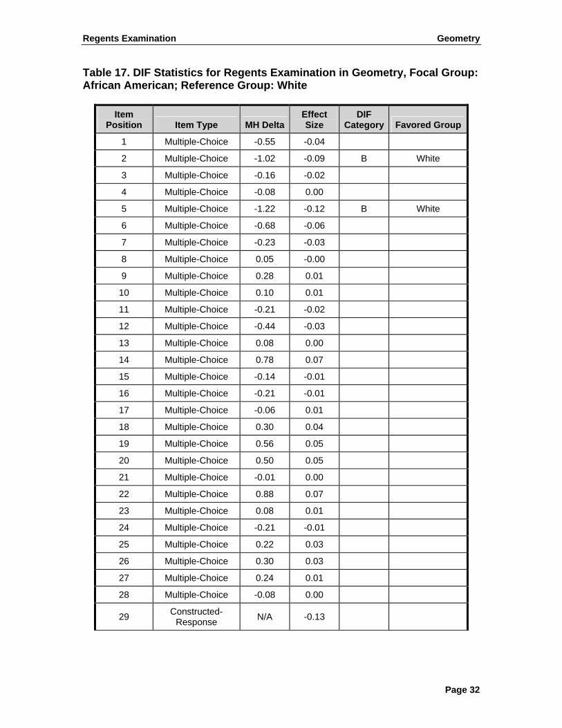
Table 8 reports reliability estimates and SEM (on raw score metric) for different testing populations: all examinees, gender groups (female and male), ethnicity groups (white, African American, and Hispanic), English Language Learners (ELL), ELL Using Accommodations (ELL/SUA),Students with Disabilities (SWD), and Students with Disabilities Using Accommodations (SWD/SUA). The number of students for each group is also provided. As can be observed from the table, the reliability estimates for total group and subgroups were all reasonably high compared with the industry standards, ranging from 0.87 to 0.92.

Regents Examination Geometry
Page 11
Table 8. Reliability Estimates and SEM for Total Population and Subpopulations
Number of
Students
Raw ScoreMean
Standard Deviation Reliability SEM
All Students 19,069 54.59 17.51 0.90 5.57
Female 9,999 54.87 17.40 0.90 5.52
Male 8,694 54.60 17.50 0.90 5.61
African American 1,919 41.59 15.79 0.87 5.76
Hispanic 2,614 45.48 16.74 0.88 5.78
White 10,483 59.10 15.64 0.88 5.39
ELL 1,165 49.75 20.48 0.92 5.68
ELL/Students Using Accommodations 392 40.05 19.76 0.92 5.73
Students With Disabilities 876 44.11 17.76 0.90 5.71
Students With Disabilities/Students Using
Accommodations 838 43.83 17.68 0.90 5.71

Regents Examination Geometry
Page 12
Table 9 reports the raw scores, scale scores, Rasch proficiency estimates ( )θ , and corresponding CSEMs. Table 9. Raw-to-Scale-Score Conversion Table and Conditional SEM for the Regents Examination in Geometry
Raw Score
Scale Score Theta CSEM
Raw Score
Scale Score Theta CSEM
Raw Score
Scale Score Theta CSEM
0 0 -5.269 1.836 29 55 -0.348 0.244 58 77 1.073 0.211 1 2 -4.540 1.018 30 56 -0.289 0.242 59 77 1.118 0.212 2 5 -3.811 0.732 31 57 -0.231 0.239 60 78 1.164 0.213 3 7 -3.370 0.607 32 58 -0.174 0.237 61 78 1.209 0.215 4 10 -3.047 0.534 33 59 -0.119 0.235 62 79 1.256 0.217 5 12 -2.789 0.484 34 60 -0.064 0.233 63 79 1.303 0.219 6 15 -2.573 0.448 35 61 -0.010 0.231 64 80 1.352 0.222 7 17 -2.385 0.419 36 62 0.043 0.229 65 80 1.402 0.225 8 20 -2.219 0.397 37 62 0.095 0.227 66 81 1.453 0.229 9 22 -2.069 0.378 38 63 0.146 0.226 67 82 1.507 0.233
10 24 -1.932 0.362 39 64 0.197 0.224 68 82 1.562 0.238 11 26 -1.806 0.349 40 65 0.247 0.223 69 83 1.620 0.243 12 29 -1.688 0.337 41 66 0.296 0.222 70 84 1.681 0.250 13 31 -1.579 0.326 42 67 0.345 0.220 71 84 1.745 0.257 14 33 -1.475 0.317 43 67 0.393 0.219 72 85 1.813 0.266 15 35 -1.377 0.309 44 68 0.441 0.218 73 86 1.887 0.276 16 36 -1.284 0.301 45 69 0.488 0.217 74 87 1.966 0.287 17 38 -1.196 0.294 46 69 0.535 0.216 75 87 2.052 0.300 18 40 -1.111 0.288 47 70 0.581 0.215 76 88 2.147 0.316 19 41 -1.030 0.282 48 71 0.627 0.214 77 89 2.252 0.334 20 43 -0.951 0.277 49 71 0.673 0.213 78 90 2.370 0.355 21 45 -0.876 0.272 50 72 0.718 0.212 79 91 2.505 0.380 22 46 -0.803 0.268 51 73 0.763 0.212 80 92 2.661 0.412 23 47 -0.732 0.264 52 73 0.808 0.211 81 93 2.847 0.452 24 49 -0.664 0.260 53 74 0.852 0.211 82 94 3.075 0.506 25 50 -0.597 0.256 54 74 0.896 0.210 83 96 3.370 0.584 26 51 -0.533 0.253 55 75 0.940 0.210 84 97 3.783 0.713 27 52 -0.469 0.250 56 75 0.985 0.210 85 98 4.485 1.005 28 54 -0.408 0.247 57 76 1.029 0.211 86 100 5.187 1.829

Regents Examination Geometry
Page 13
Classification Accuracy
Every test administration will result in some examinee classification error because of the limitations of educational measurement. Several elements used in test construction and in the roles for establishing cut scores can assist in minimizing these errors. However, it is still important to investigate reliability of classification.
The Rasch model was the IRT model used to carry out the item parameter estimation and examinee proficiency estimation for the Regents examinations. Some advantages of this IRT model include treating examinee proficiency as continuous, rather than discrete, and producing a 1-to-1 correspondence between raw scores and proficiency estimates. When the Rasch model is applied to calibrate test data, a proficiency estimate will be assigned to a given examinee on the basis of the items the examinee got correct. The estimation of proficiency is also prone to error, which is the Conditional Standard Error of Measurement. Because of the CSEM, examinees whose proficiency estimates are near a cut score may be prone to misclassification. The classification reliability index calculated in the following section is a way to accommodate the measurement error and how that may affect examinee classification. This classification reliability index is based on the errors related to measurement limitations.
As can be observed in Table 9, the CSEMs tend to be relatively large at the two extremes of the distribution and relatively small in the middle. Because there are two cut scores associated with this 86 raw score point test, the cut scores are likely to be in the middle of the raw score distributions, as were cut scores for scale scores 65 and 85, where the CSEMs tend to be relatively small.
To calculate the classification reliability index under the Rasch model for a given ability scoreθ , the observed score θ̂ is expected to be normally distributed with a mean of θ and a standard deviation of ( )SE θ (the SEM associated with the given )θ . The expected proportion of examinees with true scores in any particular level is
PropLevel( ) ( )
db a
c
cut
kcut
cut cutSE SE
θ
θ
θ θ
θ
θ θ θ μφ φ ϕθ θ σ=
− −⎛ ⎞⎛ ⎞ ⎛ ⎞ −⎛ ⎞= −⎜ ⎟⎜ ⎟ ⎜ ⎟ ⎜ ⎟⎝ ⎠⎝ ⎠ ⎝ ⎠⎝ ⎠
∑ ,
where
acutθ and
bcutθ are Rasch scale points representing the score boundaries
for levels of observed scores, c
cutθ and d
cutθ are the Rasch scale points representing score boundaries for levels of true scores, φ is the cumulative distribution function of the achievement level boundaries, and ϕ is the normal density function associated with the true scores (Rudner, 2005).

Regents Examination Geometry
Page 14
Because the Rasch model preserves the shape of the raw score distribution, which may not necessarily be normal, Pearson recommends that ϕ be replaced with the observed relative frequency distribution of θ . Some of the score boundaries may be unobserved. For example, the theoretical lower bound of Level 1 is −∞ . For practical purposes, boundaries with unobserved values can be substituted with reasonable theoretical values (–10 for lower bound of Level 1 and +10 for upper bound of Level 3).
To compute classification reliability, the proportions were computed for all the cells of a 3-by-3 classification table for the test, with the rows representing theoretical true percentages of examinees in each achievement level and the columns representing the observed percentages.
Observed 1 2 3 True 4 5 6 7 8 9
For example, suppose the cut scores are 0.5 and 1.2 on the θ scale for the 3
levels. To compute the proportion in cell 4 (observed Level 1, with scores from –10 to 0.5; true Level 2, with scores from 0.5 to 1.2), the following formula will be used:
1.2
.5
0.5 10PropLevel( ) ( )k SE SEθ
θ θ θ μφ φ ϕθ θ σ=
⎛ ⎞⎛ ⎞ ⎛ ⎞− − − −⎛ ⎞= −⎜ ⎟ ⎜ ⎟⎜ ⎟ ⎜ ⎟ ⎝ ⎠⎝ ⎠ ⎝ ⎠⎝ ⎠∑ .
Table 10 reports the percentages of students in each of the categories. The
sum of the diagonal entries (cells 1, 5, and 9, shaded in the table) represents the classification accuracy index for the test. The total percentage of students being classified accurately, on the basis of the model, was therefore 87.6%. At the proficiency cut (65), the false positive rate was 4.6% and the false negative rate was 1.3%, according to the model used. Table 10. Classification Accuracy Table.2 Score Range 0–64 65–84 85–100 True
0–64 19.5% 4.6% 0.0% 24.1%
65–84 1.3% 49.9% 3.5% 54.7%
85–100 0.0% 2.4% 18.2% 20.6%
Observed 20.8% 56.9% 21.7% 99.4%
2 Because of the calculation and the use of +10 and − 10 as cutoffs at the two extremes, the overall sum of true and observed was not always 100%, but it should be very close to 100%.

Regents Examination Geometry
Page 15
Validity
Validity is the process of collecting evidence to support inferences made with assessment results. In the case of the Regents examinations, the score use is applied to knowledge and understanding of the New York State content standards. Any correct use of the test scores is evidence of test validity.
Content and Curricular Validity
The Regents examinations are criterion-referenced assessments. That is, each assessment is based on an extensive definition of the content it assesses and its match to the content standards. Therefore, the Regents examinations are content-based and directly aligned to the statewide content standards. Consequently, the Regents examinations demonstrate good content validity. Content validity is a type of test validity that addresses whether the test adequately samples the relevant material it purports to cover.
Relation to Statewide Content Standards The development of the Regents Examination in Geometry includes
committees of educators from across the New York State, NYSED assessment and curriculum specialists and content developers from its test development contractor, Riverside Publishing Company. A sequential review process has been put in place by assessment and curriculum experts at NYSED and Riverside. Such an iterative process provides many opportunities for these assessment professionals to offer and implement suggestions for improving or eliminating items and to offer insights into the interpretation of the statewide content standards for the test. These review committees participate in this process to ensure the test content validity of the Regents examinations and the quality of the assessment.
In addition to providing information on the difficulty, appropriateness, and fairness of these items, committee members provide a needed check on the alignment between the items and the content standards they are intended to measure. When items are judged to be relevant—that is, representative of the content defined by the standards—this provides evidence to support the validity of inferences made (regarding knowledge of this content) with Regents examination results. When items are judged to be inappropriate for any reason, the committee can suggest either revisions (e.g., reclassification or rewording) or elimination of the item from the item pool. Items that are approved by the content review committee are later field tested to allow for the collection of performance data. In essence, these committees review and verify the alignment of the test items with the objectives and measurement specifications to ensure that the items measure appropriate content. They also provide insights into the quality of the items, including making sure the items are well-written, ensuring the accuracy of answer keys, providing evaluation criteria for CR items, etc. The nature and

Regents Examination Geometry
Page 16
specificity of these review procedures provide strong evidence for the content validity of the Regents Examination in Geometry.
Educator Input New York State educators provide valuable input on the content and the
match between the items and the statewide content standards. In addition, many current and former New York State educators work as independent contractors to write items specifically to measure the objectives and specifications of the content standards for the Regents examinations. Using varied sources of item writers provides a system of checks and balances for item development and review that reduces single-source bias. Because many people with different backgrounds write the items, it is less likely that items will suffer from a bias that might occur if items were written by a single author. This direct input from educators provides confirmation of the content validity of the Regents examinations.
Test Developer Input The assessment experts at NYSED and their test development contractor,
Riverside Publishing Company, provide a history of test-building experience, including content-related expertise. The input and review by these assessment professionals provide further support that the item is an accurate measure of the intended objective. As can be observed from Table 6, items are selected not only on the basis of their statistical properties, but also on the basis of their representation of the content standards. The same content specification and coverage are followed across all forms of the same assessment. These reviews and special efforts in test development offer additional evidence for the content validity of the Regents examinations.
Construct Validity
The term construct validity refers to the degree to which the test score is a measure of the characteristic (i.e., construct) of interest. A construct is an individual characteristic that is assumed to exist to explain some aspect of behavior (Linn & Gronlund, 1995). When a particular individual characteristic is inferred from an assessment result, a generalization or interpretation in terms of a construct is being made. For example, problem solving is a construct. An inference that students who master the mathematical reasoning portion of an assessment are good problem solvers implies an interpretation of the results of the assessment in terms of a construct. To make such an inference, it is important to demonstrate that this is a reasonable and valid use of the results.
The American Psychological Association provides the following list of possible sources for internal structure validity evidence (AERA, APA, & NCME, 1999):

Regents Examination Geometry
Page 17
• High intercorrelations among assessment items or tasks, attesting that the items are measuring the same trait, such as a content objective, sub-domain, or construct
• Substantial relationships between the assessment results and other measures of the same defined construct
• Little or no relationship between the assessment results and other measures that are clearly not those of the defined construct
• Substantial relationships between different methods of measurement regarding the same defined construct
• Relationships to non-assessment measures of the same defined construct
As previously mentioned, internal consistency also provides evidence of construct validity. The higher the internal consistency, or the reliability of the test scores, the more consistent the items are toward measuring a common underlying construct. In the previous section, it was observed that the reliability estimates for the assessment were reasonably high, providing positive evidence for the construct validity of the assessment.
The collection of construct-related evidence is a continuous process. Five current metrics of construct validity for the Regents examinations are the item point biserial correlations, Rasch fit statistics, intercorrelation among content strands, principal component analysis of the underlying construct, and differential item functioning (DIF) check. Validity evidence in each of these metrics is described and presented below.
Item-Total Correlation Item-total correlations provide a measure of the congruence between the way
an item functions and our expectations. Typically, we expect students with relatively high ability (i.e., those who perform well on the Regents examinations overall) to answer items correctly, and students with relatively low ability (i.e., those who perform poorly on the Regents examinations overall) to answer items incorrectly. If these expectations are accurate, the point biserial (i.e., item-total) correlation between the item and the total test score will be high and positive, indicating that the item is a good discriminator between high-performing and low-performing students. A correlation value above 0.20 is considered acceptable; a correlation value above 0.30 is considered moderately good, and values closer to 1.00 indicate superb discrimination. A test consisting of maximally discriminating items will maximize internal consistency reliability. Correlation is a mathematical concept; therefore, it is not free from misinterpretation. Often, when an item is very easy or very difficult, the point biserial correlation will be artificially deflated. For example, an item with a p-value of 99 may have a correlation of only 0.05. This does not mean that this is a bad item. The low correlation can simply be a side effect of the item difficulty. Since the item is extremely easy for everyone, not just for high-scoring students, the item is not differentiating high-performing students

Regents Examination Geometry
Page 18
from low-performing students; hence, it has low discriminating power. Because of these potential misinterpretations of the correlation, it is important to remember that the point biserial should not be used alone to determine the quality of an item.
Assuming that the total test score represents the extent to which a student possesses the construct being measured by the test, high point biserial correlations indicate that the tasks on the test require this construct to be answered correctly. Table 11 reports the point biserial correlation values for each of the items on the test. As can be observed from this table, all but two items had point biserial values of at least 0.20. Overall, it seems that all the items on the test were performing well in terms of differentiating high-performing students from low-performing students and measuring toward a common underlying construct.
Rasch Fit Statistics In addition to item point biserials, Rasch fit statistics also provide evidence of
construct validity. The Rasch model is unidimensional. Therefore, statistics showing the model-to-data fit also provide evidence that each item is measuring the same unidimensional construct. The mean square fit (MNSQ) statistics are used to determine whether items are functioning in a way that is congruent with the assumptions of the Rasch model. Under these assumptions, how a student will respond to an item depends on the proficiency of the student and the difficulty of the item, both of which are on the same measurement scale. If an item is as difficult as a student is able, the student will have a 50% chance of getting the item correct. If a student is more able than an item is difficult, under the assumptions of the Rasch model, that student has a greater than 50% chance of correctly answering the item. On the other hand, if the item is more difficult than the student is able, he or she has a less than 50% chance of correctly responding to the item. Rasch fit statistics estimate the extent to which an item is functioning in this predicted manner. Items showing a poor fit with the Rasch model typically have values outside the range of –1.3 to 1.3.
Items may not fit the Rasch model for several reasons, all of which relate to students responding to items in unexpected ways. For example, if an item appears to be easy, but consistently solicits an incorrect response from high-performing students, the fit value will likely be outside the range. Similarly, if a difficult item is answered correctly by many low-performing students, the fit statistics will not perform well. In most cases, the reason that students respond in unexpected ways to a particular item is unclear. However, it is occasionally possible to determine the cause of an item’s misfit values by reexamining the item and its distracters. For example, if several high-performing students miss an easy item, reexamination of the item may show that it actually has more than one correct response. Two response types of MNSQ values are presented in Table 11, INFIT and OUTFIT. MNSQ OUTFIT values are sensitive to outlying observations. Consequently, OUTFIT values will be outside the range when students perform unexpectedly on items that are far from their ability level—for example, easy items for which high-

Regents Examination Geometry
Page 19
performing students answer incorrectly and difficult items for which low-performing students answer correctly.

Regents Examination Geometry
Page 20
Table 11. Rasch Fit Statistics for All Items on Test
Item Position
Item Type
INFIT MNSQ
OUTFIT MNSQ
Point Biserial
Item Mean
1 Multiple-Choice 0.93 0.61 0.28 1.91 2 Multiple-Choice 0.92 0.62 0.29 1.90 3 Multiple-Choice 0.95 0.80 0.33 1.77 4 Multiple-Choice 0.93 0.75 0.37 1.75 5 Multiple-Choice 0.94 0.81 0.36 1.72 6 Multiple-Choice 0.96 0.99 0.33 1.68 7 Multiple-Choice 0.93 0.81 0.44 1.49 8 Multiple-Choice 1.00 0.97 0.36 1.38 9 Multiple-Choice 1.03 1.12 0.29 1.55 10 Multiple-Choice 0.87 0.77 0.49 1.47 11 Multiple-Choice 1.08 1.16 0.26 1.48 12 Multiple-Choice 0.99 0.94 0.36 1.50 13 Multiple-Choice 0.99 1.00 0.38 1.00 14 Multiple-Choice 0.87 0.75 0.50 1.44 15 Multiple-Choice 1.15 1.23 0.23 1.08 16 Multiple-Choice 1.00 0.99 0.38 1.11 17 Multiple-Choice 1.06 1.05 0.32 1.20 18 Multiple-Choice 0.96 0.92 0.41 1.31 19 Multiple-Choice 0.93 0.86 0.45 1.30 20 Multiple-Choice 1.17 1.27 0.21 0.96 21 Multiple-Choice 0.86 0.80 0.52 1.30 22 Multiple-Choice 0.87 0.70 0.49 1.57 23 Multiple-Choice 1.20 1.37 0.17 0.78 24 Multiple-Choice 1.14 1.21 0.24 0.95 25 Multiple-Choice 1.19 1.33 0.19 0.84 26 Multiple-Choice 1.12 1.19 0.26 0.79 27 Multiple-Choice 0.96 0.98 0.41 0.82 28 Multiple-Choice 0.97 1.12 0.36 0.64
29 Constructed-Response 0.95 1.05 0.50 1.56
30 Constructed-Response 1.04 1.07 0.49 1.55
31 Constructed-Response 0.87 0.83 0.62 1.35
32 Constructed-Response 0.94 0.95 0.58 1.20
33 Constructed-Response 0.84 0.80 0.65 1.22
34 Constructed-Response 0.92 0.90 0.56 1.50
35 Constructed-Response 1.08 1.18 0.67 2.41
36 Constructed-Response 1.03 1.05 0.69 2.32
37 Constructed-Response 0.95 0.98 0.71 1.73
38 Constructed-Response 1.24 1.35 0.70 3.10

Regents Examination Geometry
Page 21
MNSQ INFIT values are sensitive to behaviors that affect students’ performance on items near their ability estimates. Therefore, high INFIT values would occur if a group of students of similar ability consistently responded incorrectly to an item at or around their estimated ability. For example, under the Rasch model, the probability of a student with an ability estimate of 1.00 responding correctly to an item with a difficulty of 1.00 is 50%. If several students at or around the 1.00 ability level consistently miss this item such that only 20% get the item correct, the fit statistics for these items are likely to be outside the typical range. Mis-keyed items or items that contain cues to the correct response (i.e., students get the item correct regardless of their ability) may elicit high INFIT values as well. In addition, tricky items, or items that may be interpreted to have double meaning, may elicit high INFIT values.
On the basis of the results reported in Table 11, items 23, 25, and 38 had relatively high INFIT/OUTFIT statistics. The fit statistics for the rest of the items were all reasonably good. It appears that the fit of the Rasch model was good for this test.
Correlation among Content Strands There are six content strands within the core curriculum to which items are
aligned on this examination. The number of items associated with the content strands ranged from two items to 17 items. Content judgment was made when classifying items into each of the content strands. To assess the extent to which all items aligned with the content strands are assessing the same underlying construct, a correlation matrix was computed. First, the total raw scores were computed for each content strand by summing up the items within the strand. Next, correlations were computed. Table 12 presents the results. Table 12. Correlation among Content Strands
Geometric Relationships Constructions Locus
Informal and
Formal Proofs
Transformational Geometry
Coordinate Geometry
Geometric Relationships 1.00 0.38 0.37 0.54 0.43 0.52
Constructions 1.00 0.41 0.58 0.45 0.54
Locus 1.00 0.61 0.50 0.56
Informal and Formal Proofs 1.00 0.69 0.79
Transformational Geometry 1.00 0.65
Coordinate Geometry 1.00

Regents Examination Geometry
Page 22
As can be observed from Table 12, the correlations between the six content strands ranged from 0.37 (between content strands Locus and Geometric Relationships) to 0.79 (between Coordinate Geometry and Informal and Formal Proofs). This is another empirical piece of evidence suggesting that the content strands are measuring a common underlying construct.
Correlation among Item Types
Two types of items were used on the Regents Examination in Geometry: multiple-choice and constructed-response. Table 13 presents a correlation matrix (based on raw scores within each item type) to show the extent to which these two item types assessed the same underlying construct. As can be observed from the table, the correlations seem reasonably high. The high correlations between these two item types as well as between each item type and the total test is an indication of construct validity. Table 13. Correlation among Item Types and Total Test
Multiple-Choice Constructed-Response Total
Multiple-Choice 1.00 0.81 0.96
Constructed-Response 1.00 0.94
Total 1.00
Principal Component Analysis As previously mentioned, the Rasch model (Partial Credit Model, or PCM, for
CR items) was used to conduct calibration for the Regents examinations. The Rasch model is a unidimensional IRT model. Under this model, only one underlying construct is assumed to influence students’ responses to items. To check whether only one dominant dimension exists in the assessment, exploratory principal component analysis was conducted on the students’ item responses to further observe the underlying structure. Factor analysis was conducted on the item response matrix for different testing populations: all examinees, gender groups (female and male), ethnicity groups (African American, Hispanic, and white), ELL, ELL Using Accommodations (ELL/SUA), SWD, and SWD Using Accommodations (SWD/SUA). Only factors with eigenvalues greater than 1 were retained, a criteria proposed by Kaiser (1960). A scree plot was also developed (Cattell, 1966) to graphically display the relationship between factors with eigenvalues exceeding 1. Cattell suggests that when the scree plot appears to level off it is an indication that the number of significant factors has been reached. Table 14 reports the eigenvalues computed for each of the factors (only factors with eigenvalues exceeding 1 were kept and included in the table). Figure 1 shows the scree plot.

Regents Examination Geometry
Page 23
Table 14. Factors and Their Eigenvalues
Eigenvalue
Factor
1 Factor
2 Factor
3 Factor
4 Factor
5 Factor
6 Factor
7 Factor
8 Factor
9 Factor
10 Total
All Students 8.92 1.43 1.16 1.01 12.52
Female 8.96 1.40 1.12 1.02 12.51
Male 8.81 1.48 1.17 1.02 1.01 13.50
African American 7.49 1.37 1.23 1.12 1.11 1.09 1.08 1.04 1.01 1.00 17.54
Hispanic 7.93 1.41 1.22 1.11 1.08 1.04 1.00 14.79
White 7.81 1.31 1.22 1.04 1.01 12.40
ELL 10.90 1.55 1.18 1.16 1.05 1.03 16.86
ELL/SUA 10.19 1.64 1.36 1.24 1.19 1.16 1.13 1.07 1.05 1.01 21.04
SWD 8.96 1.49 1.25 1.17 1.16 1.13 1.08 1.03 1.01 18.27
SWD/SUA 8.91 1.49 1.25 1.17 1.15 1.14 1.09 1.03 1.02 18.26
Proportion
Factor
1 Factor
2 Factor
3 Factor
4 Factor
5 Factor
6 Factor
7 Factor
8 Factor
9 Factor
10
All Students 0.71 0.11 0.09 0.08
Female 0.72 0.11 0.09 0.08
Male 0.65 0.11 0.09 0.08 0.08
African American 0.43 0.08 0.07 0.06 0.06 0.06 0.06 0.06 0.06 0.06
Hispanic 0.54 0.10 0.08 0.08 0.07 0.07 0.07
White 0.63 0.11 0.10 0.08 0.08
ELL 0.65 0.09 0.07 0.07 0.06 0.06
ELL/SUA 0.48 0.08 0.06 0.06 0.06 0.06 0.05 0.05 0.05 0.05
SWD 0.49 0.08 0.07 0.06 0.06 0.06 0.06 0.06 0.06
SWD/SUA 0.49 0.08 0.07 0.06 0.06 0.06 0.06 0.06 0.06

Regents Examination Geometry
Page 24
In Table 14, there are up to ten factors with eigenvalues exceeding 1. For all students, the dominant factor has an eigenvalue of 8.92, accounting for 71% of the variance among factors with loadings exceeding 1, whereas the other factors had eigenvalues around 1. After the first and second factors, the scree plot leveled off. The scree plot also demonstrates the large magnitude of the first factor, indicating that the items on the test are measuring toward one dominant common factor. This is another piece of empirical evidence that the test has 1 dominant underlying construct and the IRT unidimensionality assumption is met. Also, the single dominant factor for each student subgroup can be observed from Table 14. Note that for some subgroups, such as ELL groups, the sample size is much smaller compared to the rest of the groups of interest and therefore, the results may contain more error. But still, the dominancy of the first factor is apparent based on the results.
0
2
4
6
8
10
12
1 2 3 4 5 6 7 8 9 10
Factor
Eig
enva
lue
All Students
Female
Male
African American
Hispanic
White
ELL
ELL/SUA
SWD
SWD/SUA
Figure 1. Scree Plot for Principal Component Analysis of Items on the Regents Examination in Geometry
Validity Evidence for Different Student Populations The primary evidence for the validity of the Regents examinations lies in the
content being measured. Since the test assesses the statewide content standards that are recommended to be taught to all students, the test is not more valid or less valid for use with one subpopulation of students relative to another. Because the Regents examinations measure what is recommended be taught to all students and are given under the same standardized conditions to all students, the tests have the same validity for all students. Moreover, great care has been taken to ensure that the items that make up the Regents examinations are fair and representative of the content domain expressed in the content standards. Additionally, much scrutiny is applied to the items and their possible impact on

Regents Examination Geometry
Page 25
minority or subpopulations in New York State. Every effort is made to eliminate items that may have ethnic or cultural biases. For example, content review and bias review are routinely conducted as part of the item review process, to eliminate any potential elements in the items that may unfairly advantage subpopulations of students.
Besides these content-based efforts that are routinely put forth in the test
development process, statistical procedures are employed to observe whether, on the basis of data, there exists possibly unfair treatment of different populations. The differential item functioning (DIF) analysis was carried out on the data collected from the June 2010 administration. DIF statistics are used to identify items for which members of a focal group have a different probability of getting the items correct than members of a reference group, after the groups have been matched on ability level on the test. In the DIF analyses, the total raw score on the operational items is used as an ability-matching variable. Four comparisons were made for each item because the same DIF analyses are typically conducted for the other New York State assessments:
• males versus females • white versus African American • white versus Hispanic • high need versus low need
For the MC items, the Mantel-Haenszel Delta (MHD) DIF statistics were computed (Dorans and Holland, 1992). The DIF null hypothesis for the Mantel-Haenszel method can be expressed as
0 : MH =( / ) /( / ) 1, 1,...,rm rm fm fmH P Q P Q m Mα = = ,
where rmP refers to the proportion of students correctly answering the item in the reference group at proficiency level m and rmQ refers to the proportion of students incorrectly answering the item in the reference group at proficiency level m . fmP and fmQ are defined similarly for the focal group. Holland and Thayer (1985) converted α into a difference in deltas via the following formula:
2.35ln(MH )MHD α= − , The following three categories were used to classify test items in three levels of DIF for each comparison: negligible DIF (A), moderate DIF (B), and large DIF (C). An item is flagged if it exhibits category B or C of DIF, using the following rules derived from the National Assessment of Educational Progress (NAEP) guidelines (Allen, Carlson, and Zalanak 1999):

Regents Examination Geometry
Page 26
Rules Descriptions Category
Rule 1 • MHD3 not significant from 0
or • |MHD| < 1.0
A
Rule 2
• MHD is significantly different from 0 and {|MHD| ≥ 1.0 and < 1.5} or
• MHD is not significantly different from 0 and |MHD| ≥ 1.0
B
Rule 3 • |MHD| ≥ 1.5 and is significantly different from 0 C
The effect size of the standardized mean difference (SMD) was used to flag the DIF for the CR items. The SMD reflects the size of the differences in performance on CR items between student groups matched on the total score. The following equation defines SMD:
Fk Fk Fk Rkk k
SMD w m w m= −∑ ∑ ,
where /Fk F k Fw n n+ ++= is the proportion of focal group members who are at the k th stratification variable, (1/ )Fk F k km n F+= is the mean item score for the focal group in the k th stratum, and (1/ )Rk R k km n R+= is the analogous value for the reference group. In words, the SMD is the difference between the unweighted item mean of the focal group and the weighted item mean of the reference group. The weights applied to the reference group are applied so that the weighted number of reference group students is the same as the weighted number of focal group students (within the same ability group). The SMD is divided by the total group item standard deviation to get a measure of the effect size for the SMD using the following equation:
SMDEffect Size=SD
.
The SMD effect size allows each item to be placed into one of three categories: negligible DIF (AA), moderate DIF (BB), or large DIF (CC). The following rules are applied for the classification. Only categories BB and CC were flagged in the results.
3 Note: The MHD is the ETS delta scale for item difficulty, where the natural logarithm of the common odds ratio is multiplied by –(4/1.7).

Regents Examination Geometry
Page 27
Rules Descriptions Category
Rule 1 • If the probability is >0.05 or |Effect Size| is ≤ 0.17 AA
Rule 2 • If the probability is < 0.05
and if 0.17<|Effect Size|≤0.25
BB
Rule 3 • If the probability is <0.05 and if |Effect Size| is >0.25 CC
For MC and CR items, the favored group is indicated if an item was flagged.
Tables 15–18 report DIF analysis for gender, ethnicity, and socio-economic status subpopulations. The sample sizes used for each of the subpopulations are reported in Table 8. When MHD values are positive, the focal group had a better odds ratio against the reference group; when the MHD values are negative, the reference group had a better odds ratio against the focal group. Similarly, when the SMD effect size values are positive, it is an indication that, at the same proficiency level, the focal group is performing better than the reference group on the item; when the SMD effect size values are negative, the reference group is performing better when the proficiency of the students is controlled.
Table 15 reports the DIF analysis for gender groups. The male group was treated as the reference group, and the female group was treated as the focal group. As can be observed from the table, one item was flagged for moderate DIF values (items 5 and 15). Both favored the reference group, the male group.
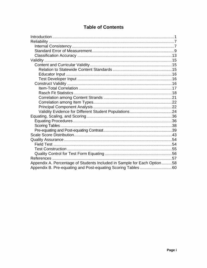
Tables 16 and 17 report the DIF analyses for ethnicity groups. The white student group was treated as the reference group. In Table 16, the Hispanic student group was treated as the focal group and the DIF statistics reported; in Table 17, the African American student group was treated as the focal group and the DIF statistics reported. One item (item 2) in Table 16 was flagged for significant DIF value favoring the white group. Two items (items 2 and 5) in Table 17 were flagged for moderate DIF favoring the white group.
Table 18 reports the DIF analysis for the high need category versus the low need category. N/RC based on the schools was used as the identification variable. The focal group is the low need group, with N/RC values being 5 and 6; the reference group is the high need group, with N/RC values being 1–4. The sample size for the high need group was 8,030 and for the low need group was 9,078. On the basis of the results presented in Table 18, one item (item 2) was flagged for moderate DIF value favoring the low need group, one item (item 6) was flagged for significant DIF value favoring the low need group, and one item (item 19) was flagged for moderate DIF favoring the high need group.

Regents Examination Geometry
Page 28
Table 15. DIF Statistics for the Regents Examination in Geometry, Focal Group: Female; Reference Group: Male
Item Position Item Type MH Delta
Effect Size
DIF Category
Favored Group
1 Multiple-Choice -0.32 -0.01
2 Multiple-Choice -0.54 -0.02
3 Multiple-Choice 0.06 0.00
4 Multiple-Choice 0.12 0.01
5 Multiple-Choice -1.04 -0.06 B Male
6 Multiple-Choice 0.29 0.02
7 Multiple-Choice -0.35 -0.03
8 Multiple-Choice -0.05 -0.00
9 Multiple-Choice 0.20 0.02
10 Multiple-Choice -0.12 -0.01
11 Multiple-Choice -0.28 -0.02
12 Multiple-Choice 0.07 0.01
13 Multiple-Choice -0.25 -0.02
14 Multiple-Choice 0.72 0.05
15 Multiple-Choice -1.09 -0.11 B Male
16 Multiple-Choice -0.90 -0.08
17 Multiple-Choice -0.11 -0.01
18 Multiple-Choice -0.04 -0.00
19 Multiple-Choice 0.05 0.00
20 Multiple-Choice -0.04 -0.00
21 Multiple-Choice 0.55 0.04
22 Multiple-Choice 0.46 0.03
23 Multiple-Choice -0.20 -0.02
24 Multiple-Choice -0.59 -0.06
25 Multiple-Choice 0.22 0.02
26 Multiple-Choice -0.17 -0.02
27 Multiple-Choice 0.11 0.01
28 Multiple-Choice -0.42 -0.03
29 Constructed-Response N/A 0.03

Regents Examination Geometry
Page 29
Table 15. DIF Statistics for the Regents Examination in Geometry, Focal Group: Female; Reference Group: Male, Continued
Item Position Item Type MH Delta
Effect Size
DIF Category Favored Group
30 Constructed-Response N/A 0.00
31 Constructed-Response N/A 0.01
32 Constructed-Response N/A -0.01
33 Constructed-Response N/A -0.01
34 Constructed-Response N/A 0.03
35 Constructed-Response N/A 0.02
36 Constructed-Response N/A 0.08
37 Constructed-Response N/A 0.05
38 Constructed-Response N/A -0.01

Regents Examination Geometry
Page 30
Table 16. DIF Statistics for Regents Examination in Geometry, Focal Group: Hispanic; Reference Group: White
Item Position Item Type MH
Delta Effect Size DIF
Category Favored Group
1 Multiple-Choice -0.24 -0.01
2 Multiple-Choice -1.56 -0.11 C White
3 Multiple-Choice -0.13 -0.01
4 Multiple-Choice 0.38 0.04
5 Multiple-Choice -0.88 -0.08
6 Multiple-Choice -0.81 -0.06
7 Multiple-Choice -0.08 -0.01
8 Multiple-Choice -0.01 -0.01
9 Multiple-Choice -0.26 -0.04
10 Multiple-Choice -0.27 -0.02
11 Multiple-Choice -0.22 -0.02
12 Multiple-Choice -0.10 0.00
13 Multiple-Choice 0.04 0.00
14 Multiple-Choice 0.28 0.03
15 Multiple-Choice 0.07 0.01
16 Multiple-Choice -0.08 0.00
17 Multiple-Choice -0.02 -0.00
18 Multiple-Choice 0.74 0.08
19 Multiple-Choice 0.74 0.07
20 Multiple-Choice 0.23 0.02
21 Multiple-Choice 0.34 0.03
22 Multiple-Choice 0.49 0.04
23 Multiple-Choice 0.13 0.01
24 Multiple-Choice -0.08 -0.00
25 Multiple-Choice 0.03 0.00
26 Multiple-Choice 0.19 0.02
27 Multiple-Choice 0.05 0.00
28 Multiple-Choice -0.11 0.00
29 Constructed-Response N/A -0.10

Regents Examination Geometry
Page 31
Table 16. DIF Statistics for Regents Examination in Geometry, Focal Group: Hispanic; Reference Group: White, Continued
Item Position Item Type MH
Delta Effect Size
DIF Category
Favored Group
30 Constructed-Response N/A -0.02
31 Constructed-Response N/A -0.01
32 Constructed-Response N/A -0.08
33 Constructed-Response N/A -0.02
34 Constructed-Response N/A 0.00
35 Constructed-Response N/A -0.01
36 Constructed-Response N/A 0.04
37 Constructed-Response N/A 0.02
38 Constructed-Response N/A -0.01
Regents Examination Geometry
Page 32
Table 17. DIF Statistics for Regents Examination in Geometry, Focal Group: African American; Reference Group: White
Item Position Item Type MH Delta
Effect Size
DIF Category Favored Group
1 Multiple-Choice -0.55 -0.04
2 Multiple-Choice -1.02 -0.09 B White
3 Multiple-Choice -0.16 -0.02
4 Multiple-Choice -0.08 0.00
5 Multiple-Choice -1.22 -0.12 B White
6 Multiple-Choice -0.68 -0.06
7 Multiple-Choice -0.23 -0.03
8 Multiple-Choice 0.05 -0.00
9 Multiple-Choice 0.28 0.01
10 Multiple-Choice 0.10 0.01
11 Multiple-Choice -0.21 -0.02
12 Multiple-Choice -0.44 -0.03
13 Multiple-Choice 0.08 0.00
14 Multiple-Choice 0.78 0.07
15 Multiple-Choice -0.14 -0.01
16 Multiple-Choice -0.21 -0.01
17 Multiple-Choice -0.06 0.01
18 Multiple-Choice 0.30 0.04
19 Multiple-Choice 0.56 0.05
20 Multiple-Choice 0.50 0.05
21 Multiple-Choice -0.01 0.00
22 Multiple-Choice 0.88 0.07
23 Multiple-Choice 0.08 0.01
24 Multiple-Choice -0.21 -0.01
25 Multiple-Choice 0.22 0.03
26 Multiple-Choice 0.30 0.03
27 Multiple-Choice 0.24 0.01
28 Multiple-Choice -0.08 0.00
29 Constructed-Response N/A -0.13

Regents Examination Geometry
Page 33
Table 17. DIF Statistics for Regents Examination in Geometry, Focal Group: African American; Reference Group: White, Continued
Item Position Item Type
MH Delta
Effect Size
DIF Category Favored Group
30 Constructed-Response N/A -0.02
31 Constructed-Response N/A -0.03
32 Constructed-Response N/A -0.07
33 Constructed-Response N/A -0.02
34 Constructed-Response N/A 0.02
35 Constructed-Response N/A -0.02
36 Constructed-Response N/A 0.07
37 Constructed-Response N/A 0.02
38 Constructed-Response N/A -0.02

Regents Examination Geometry
Page 34
Table 18. DIF Statistics for Regents Examination in Geometry, Focal Group: High Need; Reference Group: Low Need
Item Position Item Type
MH Delta
Effect Size
DIF Category Favored Group
1 Multiple-Choice 0.17 0.00
2 Multiple-Choice -1.02 -0.05 B Low Need
3 Multiple-Choice 0.46 0.04
4 Multiple-Choice 0.21 0.02
5 Multiple-Choice -0.67 -0.04
6 Multiple-Choice -1.71 -0.11 C Low Need
7 Multiple-Choice -0.21 -0.02
8 Multiple-Choice 0.19 0.02
9 Multiple-Choice -0.25 -0.03
10 Multiple-Choice -0.01 0.01
11 Multiple-Choice -0.68 -0.05
12 Multiple-Choice 0.03 0.02
13 Multiple-Choice 0.15 0.01
14 Multiple-Choice 0.73 0.06
15 Multiple-Choice 0.23 0.03
16 Multiple-Choice 0.03 0.00
17 Multiple-Choice -0.10 -0.00
18 Multiple-Choice 0.43 0.04
19 Multiple-Choice 1.03 0.08 B High Need
20 Multiple-Choice 0.07 0.01
21 Multiple-Choice 0.60 0.04
22 Multiple-Choice 0.53 0.04
23 Multiple-Choice 0.27 0.03
24 Multiple-Choice 0.21 0.02
25 Multiple-Choice 0.16 0.02
26 Multiple-Choice 0.09 0.01
27 Multiple-Choice 0.61 0.04
28 Multiple-Choice -0.20 -0.01
29 Constructed-Response N/A -0.11

Regents Examination Geometry
Page 35
Table 18. DIF Statistics for Regents Examination in Geometry, Focal Group: High Need; Reference Group: Low Need, Continued
Item Position Item Type
MH Delta
Effect Size
DIF Category Favored Group
30 Constructed-Response N/A -0.03
31 Constructed-Response N/A -0.04
32 Constructed-Response N/A -0.11
33 Constructed-Response N/A -0.05
34 Constructed-Response N/A -0.03
35 Constructed-Response N/A -0.04
36 Constructed-Response N/A 0.01
37 Constructed-Response N/A 0.02
38 Constructed-Response N/A 0.01

Regents Examination Geometry
Page 36
Equating, Scaling, and Scoring
To maintain the same performance standards across different
administrations, the statistical procedure of equating is used with the Regents examinations so that the same scale scores, even though based on a different set of items, carry the same meaning over various administrations.
There are two main kinds of equating models: the pre-equating model and the post-equating model. For regular Regents examinations, NYSED uses the pre-equating model to construct test forms of similar difficulty.
Pre-equating results were available for the items that appeared on the June 2010 Regents Examination in Geometry. These items were field-tested in the spring of 2009, together with many other items in the item bank. In these stand-alone field test sessions, the number of students taking the field test forms ranged from 700 to 800. The field test forms typically contained 10–12 items, to lighten students’ testing load in these sessions.
It has been speculated that the motivation of the students who participate in the field-testing may be lower than students who take the operational assessment, given the limited consequences of the field test and the lack of feedback (i.e., score reports) pertaining to their performance. Despite this possible lack of motivation, NYSED requirements regarding the availability of the raw-score-to-scale-score conversion chart of the recent administration dictates that a pre-equating model be employed for regular administrations of the Regents examinations. The rationale for these requirements is based primarily on the need to allow for the local scoring of the Regents examinations in the field and prompt knowledge of test results.
In this section, procedures employed in equating, scaling, and scoring for the Regents examinations are described. Furthermore, a contrast between the pre-equating results (based on the 2009 field) and the post-equating results for the operational items on the June 2010 administration of the Regents Examination in Geometry is also presented.
Equating Procedures
Under the pre-equating model, the field test forms were equated by using two designs for the Regents examinations: Equivalent Groups and Common Item. A brief description of each method follows. Equivalent Groups. For those field test forms without common items, it is assumed that the field test forms are administered to equivalent groups of students. This makes it possible to equate these forms using an equivalent group design. This is accomplished using the following steps:

Regents Examination Geometry
Page 37
Step 1: Calibrate all the field test forms allowing the item difficulties to center at
a mean value of zero. This calibration produces three valuable components for the equating and scaling process. First, this produces item parameter estimates (item difficulties and step values) for MC and CR items. Second, this produces raw-score-to-theta tables for each form. Third, this produces a mean and standard deviation of the students who take the test form.
Step 2: Using the mean-ability estimate of one of the field test forms determines an
equating constant for each of the other field test forms, which will produce a mean-ability estimate equal to that of the first form. Assuming that the samples of students who take each form are randomly equivalent, this will place the item parameters for the field test forms onto a common scale.
Step 3: Add the equating constant found in step 2 to the item difficulties and
recalibrate each test form fixing the item parameters. This will provide a check to determine whether the equating constant actually produces student ability estimates that are equal to those found in the base field test form.
Step 4: Using the item parameter estimates from the field test forms, produce a raw-
score-to-theta table for all complete forms. This will provide the tables needed to do the final scaling. Because the raw-score-to-theta tables for each form will be on the same scale, it will be possible to calculate the comparable scaled score for each raw score on the new tests.
Common Item Equating. For field test forms that contain common items, the equating is conducted in the following manner: Step 1: Calibrate one form allowing the item difficulties to center at a mean value of 0,
or use previously calibrated difficulty values if available. For the base test form, the calibration produces three valuable components for the equating and scaling process. First, this produces item parameter estimates (item difficulties and step values) for MC and CR items. Second, it produces raw-score-to-theta tables for each form. Third, this will produce a mean and standard deviation of the students who take the test form.
Step 2: Calibrate the other field test forms fixing the common item parameters to
those found in step 1. This will place the item parameters for the mini-forms onto a common scale. (Before this step, an analysis of the stability of the item-difficulty estimates for the anchor items will be performed. Items demonstrating unstable estimates will not be used as anchors.)
Step 3: Repeat steps 2 and 3 for the other field test forms. This will place the item parameters for all the field test forms onto a common scale.

Regents Examination Geometry
Page 38
Step 4: Using the item parameter estimates from step 3, produce a raw-score-to-theta table for all complete forms. This will provide the tables needed to do the final scaling. Because the raw-score-to-theta tables will be on the same scale for each form, it will be possible to calculate the comparable scale score for each raw score on the new tests.
The stability of the anchor was evaluated before being used as an anchor in the
equating. This stability check involved the examination of the displacement values provided in the BIGSTEPS/WINSTEPS output. Anchor items with displacements larger than 0.30 were “freed” in the calibration process.
The administration of the field test forms for the Regents Examination in Geometry used a spiraled design. In this design, equivalent groups of students were administered the various mini field test forms, including two anchor forms. With this design, the forms can be calibrated using the Rasch and PCM models and equated using an equivalent groups equating design as mentioned above.
The field testing was conducted in the spring of 2009. These items were then calibrated and placed onto the same scale. Operational test forms were constructed for June and August administrations in 2010 and January administration in 2011. A pre-equating procedure was employed to make the test forms as parallel as possible so that the cut scores will maintain similar magnitude across other forms.
Scoring Tables
As a result of the item analysis, each item in the bank has a Rasch difficulty that is on the same scale as all other items in the bank. As items are selected for use on the operational test forms, the average item difficulty of the test forms indicates the difficulty of the test relative to previous test forms. This relationship influences the resulting raw scores associated with the scale scores of 65 and 85.
Using equated Rasch difficulties and step values, a raw-score-to-theta (e.g., student ability) relationship is developed. Each theta represents a level of student performance needed to attain each raw score that can be compared across test forms. Using this relationship, the level of student performance needed to attain each scale score (e.g., 65 and 85) is held constant across test forms. That means that if a particular test form is more difficult than another, students are not penalized. This process of equating the scoring tables will cause an adjustment on the more difficult form and the 65 and/or 85 scale score will be assigned to a lower raw score. If a particular test form is easier than another, students are not unfairly advantaged either. This process of equating the scoring tables will also cause an adjustment on the much easier form and assign the 65 and/or 85 scale score to a higher raw score. With this adjustment, a constant expectation of student performance is maintained across test forms.

Regents Examination Geometry
Page 39
Pre-equating and Post-equating Contrast
Post-equating also was conducted, using samples collected after the June 2010 administrations of the New York State Regents Examination in Geometry, to observe how robust the pre-equating procedure was and the impact that it had on student-achievement level classifications. The following steps are used to conduct post-equating:
1. Conduct a free calibration on the operational data to obtain item parameter estimates and raw-score-to-theta conversion table.
2. The mean of the item parameters obtained from step 1 was computed 3. Equating constant (0.14) was obtained by subtracting the mean obtained at step
2 from the corresponding mean value based on pre-equating item parameters. 4. Add the equating constant to all item parameter estimates and theta estimates
obtained from operational data. 5. After step 4, post equating results were equated to the operational reporting
scale. Table 19 presents the Rasch Item Difficulties (RIDs) for the pre-equating
model, the post-equating model, and the differences between the 2 models. As can be observed from this table, the item means tended to be higher when based on operational data compared with their corresponding item means based on field-testing data. Such observation may be partly due to the separate field-testing session, in which a student’s motivation tends not to be ideal.
The average absolute difference between the RIDs was 0.34 for the 2010 administration items. The correlation between pre-equating and post-operational RIDs was 0.92. In most applications of the Rasch model, correlations between RIDs obtained between the two administrations are expected to be above 0.90 and average absolute differences are expected to be below 0.20. Thus, these results suggest some degree of dissimilarities in terms of item parameter estimates between the pre-equating and post-equating RIDs for the 2010 administration.
Scoring tables display the relationship between the raw score and theta (e.g., student ability). Specifically, the field test equated item parameters (e.g., RIDs) were used to develop the scoring table for the pre-equating model. On the other hand, the scaling constants (0.14) were added to the scoring table created by post-equating RIDs in order to place those on the same scale as was used for pre-equating.

Regents Examination Geometry
Page 40
Table 19. Contrasts between Pre-equated and Post-operational Item Parameter Estimates
Item Pre-equated Item Mean
Post -operational Item Mean
Pre-equated Item
Parameters
Post -operational
Item Parameters
Pre-Post Difference
1 1.78 1.91 -2.05 -2.57 0.52 2 1.74 1.90 -1.98 -2.42 0.44 3 1.62 1.77 -1.35 -1.44 0.09 4 1.64 1.75 -1.46 -1.32 -0.14 5 1.54 1.72 -1.29 -1.19 -0.10 6 1.36 1.68 -0.55 -0.98 0.43 7 1.32 1.49 -0.50 -0.30 -0.20 8 1.26 1.38 -0.33 0.00 -0.33 9 1.24 1.55 -0.29 -0.52 0.23
10 1.16 1.47 -0.07 -0.25 0.18 11 1.08 1.48 0.08 -0.28 0.36 12 1.06 1.50 0.22 -0.33 0.55 13 1.02 1.00 0.15 1.00 -0.85 14 1.02 1.44 0.26 -0.16 0.42 15 1.00 1.08 0.34 0.80 -0.46 16 1.00 1.11 0.17 0.74 -0.57 17 0.96 1.20 0.35 0.49 -0.14 18 0.94 1.31 0.34 0.21 0.13 19 0.94 1.30 0.34 0.22 0.12 20 0.92 0.96 0.49 1.11 -0.62 21 0.82 1.30 0.59 0.24 0.35 22 0.82 1.57 0.64 -0.58 1.22 23 0.78 0.78 0.79 1.55 -0.76 24 0.76 0.95 0.84 1.13 -0.29 25 0.74 0.84 0.94 1.39 -0.45 26 0.62 0.79 1.16 1.53 -0.37 27 0.62 0.82 1.19 1.45 -0.26 28 0.58 0.64 1.27 1.95 -0.68 29 1.33 1.56 -0.49 -0.55 0.06 30 1.18 1.55 0.04 -0.17 0.21 31 1.01 1.35 0.15 0.27 -0.12 32 0.89 1.20 0.53 0.54 -0.01 33 0.77 1.22 0.73 0.50 0.23 34 1.13 1.50 0.04 -0.13 0.17 35 1.95 2.41 0.29 0.55 -0.26 36 1.09 2.32 1.23 0.68 0.55 37 0.81 1.73 1.29 1.20 0.09 38 1.96 3.10 1.06 0.92 0.14
Figure 2 presents the scoring tables based on the 2 equating models mentioned above. The horizontal axis represents the ability estimate, and the vertical axis represents raw scores. According to the figure, the scoring tables for pre-equating and post-equating models were quite similar.

Regents Examination Geometry
Page 41
0102030405060708090
-6 -4 -2 0 2 4 6
Ability estimate
Raw
Sco
re
Pre-equating Model
Post-equating Model
Figure 2. Comparison of Relationship between Raw Score and Ability Estimates between Pre-equating Model and Post-equating Model
To further observe the impact between the two equating models, Table 20 was constructed, reporting raw score cuts and percent of students in each of the achievement levels based on the sample used for the analysis. For the identification of the cut score, the theta cuts from the standard setting were used. Because of the discrete nature of the scoring table, it is unlikely to have the theta values on the scoring table that exactly match the standard setting thetas. Therefore, the closest theta values to the standard setting values without going over were identified, and their corresponding raw scores were assigned to be the cut scores based on post-equating. Appendix B provides the comparison between the scoring tables based on pre-equating and post-equating.
As can be observed from Table 20, the raw score cut corresponding to the scale score of 65 was one point lower for the pre-equating results, resulting in about 0.36% fewer students being classified into 0–64 and 4.18% more into 65–84 based on the pre-equating model. The raw score cut corresponding to a scale score of 85 for the post-equating model was two points lower for the pre-equating model, resulting in about 2.08% more students being classified into 85-100 based on the pre-equating model..
There are some differences between the item parameter estimates as well as
scoring tables between the pre- and post-equating models. The differences were noticeable, but the differences appeared more at the higher score level than other places across the entire distribution.

Regents Examination Geometry
Page 42
Table 20. Comparisons of Raw Score Cuts and Percentages of Students in Each of the Achievement Levels between Pre-equating and Post-equating Models
Pre-equating Model
Post-equating Model
Scale Score
Raw Score Cut
Percent in Level
Raw Score Cut
Percent in Level
0–64 20.47 20.83
65–84 40 59.34 41 55.16
85–100 72 20.19 70 22.27

Regents Examination Geometry
Page 43
Scale Score Distribution
To observe how students performed on the Regents Examination in Geometry, the scale scores for the students included in the sample were analyzed. In Tables 21–29, frequency distributions are reported for all students, male and female students, white, Hispanic, and African American students, students with ELL, ELL Using Accommodations, students with low socio- economic status, SWD, SWD Using Accommodations, and grade levels. Mean and standard deviations of scale scores are also computed for all students and each of the subgroups in Table 30. Percentages of students in each of the achievement levels (0–64, 65–84, and 85–100) are reported in Table 31. Table 21. Scale Score Distribution for All Students
Scale Score Freq. Percent
Cum. Per.
Scale Score Freq. Percent
Cum. Per.
Scale Score Freq. Percent
Cum. Per.
7 1 0.01 0.01 51 140 0.73 7.49 76 758 3.98 53.689 5 0.03 0.03 52 177 0.93 8.42 77 719 3.77 57.45
11 2 0.01 0.04 54 172 0.90 9.32 78 352 1.85 59.3014 6 0.03 0.07 55 207 1.09 10.41 79 689 3.61 62.9116 3 0.02 0.09 56 206 1.08 11.49 80 733 3.84 66.7618 12 0.06 0.15 57 222 1.16 12.65 81 344 1.80 68.5620 5 0.03 0.18 58 205 1.08 13.73 82 722 3.79 72.3522 26 0.14 0.31 59 240 1.26 14.99 83 695 3.64 75.9925 15 0.08 0.39 60 242 1.27 16.26 84 332 1.74 77.7327 43 0.23 0.62 61 241 1.26 17.52 85 396 2.08 79.8129 18 0.09 0.71 62 221 1.16 18.68 86 715 3.75 83.5631 45 0.24 0.95 63 211 1.11 19.79 87 381 2.00 85.5633 28 0.15 1.10 64 199 1.04 20.83 88 653 3.42 88.9834 64 0.34 1.43 65 756 3.96 24.79 89 249 1.31 90.2936 58 0.30 1.74 66 346 1.81 26.61 90 335 1.76 92.0438 78 0.41 2.14 67 285 1.49 28.10 91 237 1.24 93.2940 79 0.41 2.56 68 647 3.39 31.50 92 297 1.56 94.8541 78 0.41 2.97 69 307 1.61 33.11 93 171 0.90 95.7443 88 0.46 3.43 70 346 1.81 34.92 95 292 1.53 97.2744 103 0.54 3.97 71 696 3.65 38.57 96 118 0.62 97.8946 97 0.51 4.48 72 375 1.97 40.54 97 242 1.27 99.1647 135 0.71 5.19 73 687 3.60 44.14 98 49 0.26 99.4249 143 0.75 5.94 74 362 1.90 46.04 100 111 0.58 100.0050 157 0.82 6.76 75 700 3.67 49.71

Regents Examination Geometry
Page 44
Table 22. Scale Score Distribution for Male Students
Scale Score Freq. Percent
Cum. Per.
Scale Score Freq. Percent
Cum. Per.
Scale Score Freq. Percent
Cum. Per.
7 1 0.01 0.01 51 62 0.71 7.58 76 337 3.88 53.749 4 0.05 0.06 52 78 0.90 8.48 77 334 3.84 57.58
11 1 0.01 0.07 54 78 0.90 9.37 78 165 1.90 59.4814 2 0.02 0.09 55 84 0.97 10.34 79 317 3.65 63.1216 2 0.02 0.12 56 82 0.94 11.28 80 322 3.70 66.8318 3 0.03 0.15 57 100 1.15 12.43 81 175 2.01 68.8420 2 0.02 0.17 58 90 1.04 13.47 82 345 3.97 72.8122 16 0.18 0.36 59 110 1.27 14.73 83 289 3.32 76.1325 7 0.08 0.44 60 99 1.14 15.87 84 149 1.71 77.8527 19 0.22 0.66 61 115 1.32 17.20 85 180 2.07 79.9229 10 0.12 0.77 62 100 1.15 18.35 86 333 3.83 83.7531 19 0.22 0.99 63 89 1.02 19.37 87 158 1.82 85.5633 19 0.22 1.21 64 104 1.20 20.57 88 299 3.44 89.0034 29 0.33 1.54 65 342 3.93 24.50 89 107 1.23 90.2336 29 0.33 1.87 66 154 1.77 26.27 90 145 1.67 91.9038 39 0.45 2.32 67 132 1.52 27.79 91 116 1.33 93.2440 37 0.43 2.75 68 293 3.37 31.16 92 136 1.56 94.8041 34 0.39 3.14 69 148 1.70 32.86 93 77 0.89 95.6943 40 0.46 3.60 70 158 1.82 34.68 95 126 1.45 97.1444 44 0.51 4.11 71 301 3.46 38.14 96 63 0.72 97.8646 45 0.52 4.62 72 175 2.01 40.15 97 107 1.23 99.0947 65 0.75 5.37 73 343 3.95 44.10 98 24 0.28 99.3749 59 0.68 6.05 74 163 1.87 45.97 100 55 0.63 100.0050 71 0.82 6.87 75 338 3.89 49.86

Regents Examination Geometry
Page 45
Table 23. Scale Score Distribution for Female Students
Scale Score Freq. Percent
Cum. Per.
Scale Score Freq. Percent
Cum. Per.
Scale Score Freq. Percent
Cum. Per.
9 1 0.01 0.01 52 97 0.97 7.95 76 404 4.04 53.0611 1 0.01 0.02 54 89 0.89 8.84 77 373 3.73 56.7914 2 0.02 0.04 55 114 1.14 9.98 78 180 1.80 58.5916 1 0.01 0.05 56 119 1.19 11.17 79 363 3.63 62.2218 9 0.09 0.14 57 112 1.12 12.29 80 400 4.00 66.2222 8 0.08 0.22 58 111 1.11 13.40 81 163 1.63 67.8525 7 0.07 0.29 59 127 1.27 14.67 82 372 3.72 71.5727 20 0.20 0.49 60 136 1.36 16.03 83 393 3.93 75.5029 8 0.08 0.57 61 123 1.23 17.26 84 180 1.80 77.3031 23 0.23 0.80 62 119 1.19 18.45 85 210 2.10 79.4033 9 0.09 0.89 63 114 1.14 19.59 86 373 3.73 83.1334 31 0.31 1.20 64 92 0.92 20.51 87 217 2.17 85.3036 26 0.26 1.46 65 397 3.97 24.48 88 345 3.45 88.7538 37 0.37 1.83 66 185 1.85 26.33 89 138 1.38 90.1340 39 0.39 2.22 67 149 1.49 27.82 90 188 1.88 92.0141 37 0.37 2.59 68 336 3.36 31.18 91 120 1.20 93.2143 44 0.44 3.03 69 154 1.54 32.72 92 159 1.59 94.8044 51 0.51 3.54 70 181 1.81 34.53 93 92 0.92 95.7246 50 0.50 4.04 71 381 3.81 38.34 95 163 1.63 97.3547 65 0.65 4.69 72 195 1.95 40.29 96 54 0.54 97.8949 78 0.78 5.47 73 333 3.33 43.62 97 133 1.33 99.2250 79 0.79 6.26 74 195 1.95 45.57 98 24 0.24 99.4651 72 0.72 6.98 75 344 3.44 49.01 100 54 0.54 100.00

Regents Examination Geometry
Page 46
Table 24. Scale Score Distribution for White Students
Scale Score Freq. Percent
Cum. Per.
Scale Score Freq. Percent
Cum. Per.
Scale Score Freq. Percent
Cum. Per.
7 1 0.01 0.01 55 67 0.64 4.45 77 452 4.31 48.179 1 0.01 0.02 56 64 0.61 5.07 78 221 2.11 50.28
22 2 0.02 0.04 57 78 0.74 5.81 79 412 3.93 54.2125 5 0.05 0.09 58 77 0.73 6.54 80 460 4.39 58.6027 4 0.04 0.12 59 88 0.84 7.38 81 235 2.24 60.8429 3 0.03 0.15 60 86 0.82 8.20 82 463 4.42 65.2631 9 0.09 0.24 61 111 1.06 9.26 83 445 4.24 69.5033 6 0.06 0.30 62 98 0.93 10.20 84 230 2.19 71.7034 14 0.13 0.43 63 73 0.70 10.89 85 257 2.45 74.1536 4 0.04 0.47 64 74 0.71 11.60 86 466 4.45 78.5938 11 0.10 0.57 65 358 3.42 15.01 87 254 2.42 81.0240 11 0.10 0.68 66 176 1.68 16.69 88 457 4.36 85.3841 8 0.08 0.75 67 132 1.26 17.95 89 175 1.67 87.0543 21 0.20 0.95 68 336 3.21 21.16 90 250 2.38 89.4344 20 0.19 1.14 69 171 1.63 22.79 91 173 1.65 91.0846 26 0.25 1.39 70 194 1.85 24.64 92 214 2.04 93.1247 34 0.32 1.72 71 382 3.64 28.28 93 121 1.15 94.2849 25 0.24 1.96 72 199 1.90 30.18 95 224 2.14 96.4150 39 0.37 2.33 73 386 3.68 33.86 96 86 0.82 97.2351 36 0.34 2.67 74 206 1.97 35.83 97 169 1.61 98.8552 66 0.63 3.30 75 395 3.77 39.60 98 37 0.35 99.2054 54 0.52 3.82 76 447 4.26 43.86 100 84 0.80 100.00

Regents Examination Geometry
Page 47
Table 25. Scale Score Distribution for Hispanic Students
Scale Score Freq. Percent
Cum. Per.
Scale Score Freq. Percent
Cum. Per.
Scale Score Freq. Percent
Cum. Per.
9 2 0.08 0.08 52 33 1.26 17.67 76 93 3.56 74.7511 1 0.04 0.11 54 50 1.91 19.59 77 69 2.64 77.3914 1 0.04 0.15 55 45 1.72 21.31 78 36 1.38 78.7716 1 0.04 0.19 56 47 1.80 23.11 79 76 2.91 81.6818 4 0.15 0.34 57 51 1.95 25.06 80 80 3.06 84.7422 10 0.38 0.73 58 42 1.61 26.66 81 29 1.11 85.8525 3 0.11 0.84 59 56 2.14 28.81 82 69 2.64 88.4927 13 0.50 1.34 60 57 2.18 30.99 83 61 2.33 90.8229 5 0.19 1.53 61 46 1.76 32.75 84 24 0.92 91.7431 15 0.57 2.10 62 38 1.45 34.20 85 28 1.07 92.8133 3 0.11 2.22 63 40 1.53 35.73 86 57 2.18 94.9934 21 0.80 3.02 64 44 1.68 37.41 87 20 0.77 95.7536 19 0.73 3.75 65 148 5.66 43.08 88 45 1.72 97.4838 23 0.88 4.63 66 61 2.33 45.41 89 10 0.38 97.8640 24 0.92 5.55 67 56 2.14 47.55 90 10 0.38 98.2441 24 0.92 6.47 68 110 4.21 51.76 91 8 0.31 98.5543 19 0.73 7.19 69 40 1.53 53.29 92 11 0.42 98.9744 30 1.15 8.34 70 50 1.91 55.20 93 11 0.42 99.3946 26 0.99 9.33 71 106 4.06 59.26 95 8 0.31 99.6947 45 1.72 11.06 72 57 2.18 61.44 96 2 0.08 99.7749 56 2.14 13.20 73 96 3.67 65.11 97 5 0.19 99.9650 43 1.64 14.84 74 58 2.22 67.33 100 1 0.04 100.0051 41 1.57 16.41 75 101 3.86 71.19

Regents Examination Geometry
Page 48
Table 26. Scale Score Distribution for African American Students
Scale Score Freq. Percent
Cum. Per.
Scale Score Freq. Percent
Cum. Per.
Scale Score Freq. Percent
Cum. Per.
9 2 0.10 0.10 51 31 1.62 19.75 74 23 1.20 76.6511 1 0.05 0.16 52 45 2.34 22.09 75 50 2.61 79.2614 1 0.05 0.21 54 37 1.93 24.02 76 66 3.44 82.7016 1 0.05 0.26 55 39 2.03 26.06 77 41 2.14 84.8418 5 0.26 0.52 56 46 2.40 28.45 78 30 1.56 86.4022 8 0.42 0.94 57 43 2.24 30.69 79 45 2.34 88.7425 3 0.16 1.09 58 46 2.40 33.09 80 39 2.03 90.7827 16 0.83 1.93 59 51 2.66 35.75 81 13 0.68 91.4529 4 0.21 2.14 60 54 2.81 38.56 82 33 1.72 93.1731 10 0.52 2.66 61 37 1.93 40.49 83 28 1.46 94.6333 14 0.73 3.39 62 50 2.61 43.10 84 10 0.52 95.1534 11 0.57 3.96 63 49 2.55 45.65 85 11 0.57 95.7336 23 1.20 5.16 64 36 1.88 47.52 86 31 1.62 97.3438 26 1.35 6.51 65 117 6.10 53.62 87 11 0.57 97.9240 18 0.94 7.45 66 48 2.50 56.12 88 16 0.83 98.7541 27 1.41 8.86 67 44 2.29 58.42 89 5 0.26 99.0143 24 1.25 10.11 68 68 3.54 61.96 90 6 0.31 99.3244 24 1.25 11.36 69 28 1.46 63.42 91 5 0.26 99.5846 30 1.56 12.92 70 37 1.93 65.35 92 5 0.26 99.8447 31 1.62 14.54 71 85 4.43 69.78 95 1 0.05 99.9049 35 1.82 16.36 72 37 1.93 71.70 96 1 0.05 99.9550 34 1.77 18.13 73 72 3.75 75.46 97 1 0.05 100.00

Regents Examination Geometry
Page 49
Table 27. Scale Score Distribution for English Language Learners
Scale Score Freq. Percent
Cum. Per.
Scale Score Freq. Percent
Cum. Per.
Scale Score Freq. Percent
Cum. Per.
14 2 0.17 0.17 54 15 1.29 20.43 76 43 3.69 61.7218 3 0.26 0.43 55 13 1.12 21.55 77 33 2.83 64.5520 1 0.09 0.52 56 19 1.63 23.18 78 10 0.86 65.4122 7 0.60 1.12 57 18 1.55 24.72 79 23 1.97 67.3825 1 0.09 1.20 58 20 1.72 26.44 80 29 2.49 69.8727 12 1.03 2.23 59 14 1.20 27.64 81 20 1.72 71.5929 5 0.43 2.66 60 17 1.46 29.10 82 33 2.83 74.4231 10 0.86 3.52 61 12 1.03 30.13 83 35 3.00 77.4233 1 0.09 3.61 62 8 0.69 30.82 84 15 1.29 78.7134 10 0.86 4.46 63 18 1.55 32.36 85 25 2.15 80.8636 9 0.77 5.24 64 13 1.12 33.48 86 40 3.43 84.2938 12 1.03 6.27 65 47 4.03 37.51 87 19 1.63 85.9240 14 1.20 7.47 66 19 1.63 39.14 88 37 3.18 89.1041 15 1.29 8.76 67 18 1.55 40.69 89 10 0.86 89.9643 11 0.94 9.70 68 31 2.66 43.35 90 15 1.29 91.2444 17 1.46 11.16 69 22 1.89 45.24 91 17 1.46 92.7046 13 1.12 12.27 70 19 1.63 46.87 92 22 1.89 94.5947 18 1.55 13.82 71 37 3.18 50.04 93 11 0.94 95.5449 14 1.20 15.02 72 24 2.06 52.10 95 20 1.72 97.2550 16 1.37 16.39 73 27 2.32 54.42 96 7 0.60 97.8551 17 1.46 17.85 74 18 1.55 55.97 97 15 1.29 99.1452 15 1.29 19.14 75 24 2.06 58.03 100 10 0.86 100.00

Regents Examination Geometry
Page 50
Table 28. Scale Score Distribution for Students with Low Socio- Economic Status
Scale Score Freq. Percent
Cum. Per.
Scale Score Freq. Percent
Cum. Per.
Scale Score Freq. Percent
Cum. Per.
7 1 0.01 0.01 51 96 1.20 12.86 76 312 3.89 66.249 4 0.05 0.06 52 103 1.28 14.15 77 270 3.36 69.60
11 2 0.02 0.09 54 111 1.38 15.53 78 134 1.67 71.2714 4 0.05 0.14 55 118 1.47 17.00 79 258 3.21 74.4816 3 0.04 0.17 56 126 1.57 18.57 80 272 3.39 77.8718 12 0.15 0.32 57 124 1.54 20.11 81 125 1.56 79.4320 5 0.06 0.39 58 113 1.41 21.52 82 261 3.25 82.6822 23 0.29 0.67 59 136 1.69 23.21 83 225 2.80 85.4825 8 0.10 0.77 60 143 1.78 24.99 84 102 1.27 86.7527 35 0.44 1.21 61 132 1.64 26.64 85 121 1.51 88.2629 17 0.21 1.42 62 118 1.47 28.11 86 230 2.86 91.1231 36 0.45 1.87 63 112 1.39 29.50 87 107 1.33 92.4533 25 0.31 2.18 64 134 1.67 31.17 88 164 2.04 94.5034 49 0.61 2.79 65 353 4.40 35.57 89 54 0.67 95.1736 43 0.54 3.33 66 171 2.13 37.70 90 65 0.81 95.9838 67 0.83 4.16 67 142 1.77 39.46 91 52 0.65 96.6340 51 0.64 4.79 68 306 3.81 43.28 92 70 0.87 97.5041 61 0.76 5.55 69 146 1.82 45.09 93 34 0.42 97.9243 61 0.76 6.31 70 161 2.00 47.10 95 56 0.70 98.6244 80 1.00 7.31 71 303 3.77 50.87 96 23 0.29 98.9046 67 0.83 8.14 72 179 2.23 53.10 97 64 0.80 99.7047 93 1.16 9.30 73 298 3.71 56.81 98 8 0.10 99.8049 93 1.16 10.46 74 158 1.97 58.78 100 16 0.20 100.0050 97 1.21 11.67 75 287 3.57 62.35

Regents Examination Geometry
Page 51
Table 29. Scale Score Distribution for Students with Disabilities
Scale Score Freq. Percent
Cum. Per.
Scale Score Freq. Percent
Cum. Per.
Scale Score Freq. Percent
Cum. Per.
7 1 0.11 0.11 52 11 1.26 20.09 76 36 4.11 75.689 2 0.23 0.34 54 22 2.51 22.60 77 39 4.45 80.14
11 1 0.11 0.46 55 11 1.26 23.86 78 8 0.91 81.0516 1 0.11 0.57 56 13 1.48 25.34 79 18 2.05 83.1118 4 0.46 1.03 57 19 2.17 27.51 80 16 1.83 84.9322 6 0.68 1.71 58 12 1.37 28.88 81 11 1.26 86.1925 4 0.46 2.17 59 17 1.94 30.82 82 24 2.74 88.9327 9 1.03 3.20 60 24 2.74 33.56 83 16 1.83 90.7529 7 0.80 4.00 61 25 2.85 36.42 84 11 1.26 92.0131 9 1.03 5.02 62 13 1.48 37.90 85 9 1.03 93.0433 6 0.68 5.71 63 18 2.05 39.95 86 10 1.14 94.1834 9 1.03 6.74 64 7 0.80 40.75 87 7 0.80 94.9836 9 1.03 7.76 65 47 5.37 46.12 88 17 1.94 96.9238 11 1.26 9.02 66 14 1.60 47.72 89 1 0.11 97.0340 4 0.46 9.47 67 12 1.37 49.09 90 12 1.37 98.4041 8 0.91 10.39 68 36 4.11 53.20 91 3 0.34 98.7443 12 1.37 11.76 69 13 1.48 54.68 92 5 0.57 99.3244 7 0.80 12.56 70 23 2.63 57.31 95 2 0.23 99.5446 10 1.14 13.70 71 33 3.77 61.07 96 1 0.11 99.6647 16 1.83 15.53 72 20 2.28 63.36 97 2 0.23 99.8949 10 1.14 16.67 73 34 3.88 67.24 100 1 0.11 100.0050 9 1.03 17.69 74 13 1.48 68.72 51 10 1.14 18.84 75 25 2.85 71.58
Regents Examination Geometry
Page 52
Table 30. Descriptive Statistics on Scale Scores for Various Student Groups
Number of
Students Percent Mean Standard Deviation
All Students 19,069 100.00 73.58 13.87
Female 9,999 52.44 73.82 13.63
Male 8,694 45.59 73.58 13.92
African American 1,919 10.06 63.25 14.31
Hispanic 2,614 13.71 66.42 14.41
White 10,483 54.97 77.20 11.57
ELL 1,165 6.11 69.08 17.50
ELL/Students Using Accommodations 392 2.06 60.37 18.81
Low SES 8,030 42.11 69.11 14.78
Students With Disabilities 876 4.59 64.79 16.29
Students With Disabilities/ Students Using Accommodations 838 4.39 64.57 16.27
Grade 9 4,966 26.04 82.18 10.92
Grade 10 10,923 57.28 72.20 12.58
Grade 11 2,293 12.02 63.64 13.87
Grade 12 262 1.37 62.03 14.37
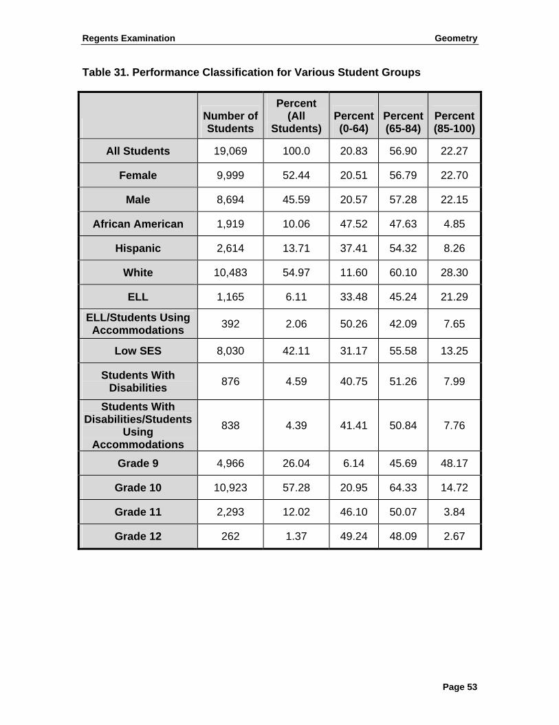
Regents Examination Geometry
Page 53
Table 31. Performance Classification for Various Student Groups
Number of Students
Percent (All
Students) Percent(0-64)
Percent (65-84)
Percent(85-100)
All Students 19,069 100.0 20.83 56.90 22.27
Female 9,999 52.44 20.51 56.79 22.70
Male 8,694 45.59 20.57 57.28 22.15
African American 1,919 10.06 47.52 47.63 4.85
Hispanic 2,614 13.71 37.41 54.32 8.26
White 10,483 54.97 11.60 60.10 28.30
ELL 1,165 6.11 33.48 45.24 21.29
ELL/Students Using Accommodations 392 2.06 50.26 42.09 7.65
Low SES 8,030 42.11 31.17 55.58 13.25
Students With Disabilities 876 4.59 40.75 51.26 7.99
Students With Disabilities/Students
Using Accommodations
838 4.39 41.41 50.84 7.76
Grade 9 4,966 26.04 6.14 45.69 48.17
Grade 10 10,923 57.28 20.95 64.33 14.72
Grade 11 2,293 12.02 46.10 50.07 3.84
Grade 12 262 1.37 49.24 48.09 2.67

Regents Examination Geometry
Page 54
Quality Assurance
The Regents examinations program and its associated data play an important role in the State accountability system as well as in many local evaluation plans. Therefore, it is vital that quality control procedures, which ensure the accuracy of student, school and district-level data and reports, are implemented. A set of quality control procedures has been developed and refined to help ensure that the testing quality assurance requirements are met or exceeded. These quality control procedures are detailed in the paragraphs that follow.
Field Test
Before items are placed on an operational test form of the Regents examinations, they have to go through several phases of reviews and field-testing to ensure the quality of the test. During field testing, items are tried out to observe their statistical behaviors. After field testing, the answer sheets are collected from students, and scanned at NYSED. Quality control procedures and regular preventative maintenance ensure that the NYSED scanner is functioning properly at all times.
To score essay items, rangefinding is conducted first to define detailed rubrics for the items. Next, scorers are trained through a set of rigorous procedures to ensure consistent ratings. The primary goal of the rangefinding meetings is to identify and select a representative sample of student responses for each item for use as exemplar papers for each of the content areas for each of the items. These responses accurately represent the range of student achievement levels described in the rubric for each item, as interpreted by the committee members in each session. Careful selection of papers during rangefinding and the subsequent compilation of anchor papers and other training materials are essential to ensuring that scoring can be conducted consistently and reliably. All the necessary steps were also taken to ensure the security of the materials.
After rangefinding, scoring supervisors and scorers are selected and trained to score field test items. Scoring supervisors had college degrees in the subject area or a related area. Supervisors had experience in scoring the subject area and demonstrated strong organizational abilities and communication skills. Each scorer possessed, at a minimum, a 4-year college degree. They were assigned to work in the most appropriate subject area based on their educational qualifications and their work or scoring experience. Scoring directors or supervisors began training by reviewing and discussing the scoring guides and anchor sets for items in a book. Scoring directors or supervisors then gave scorers practice sets, and scorers assigned scores to these sample responses. After scorers completed the set, scoring directors or supervisors reviewed and explained true scores for the practice papers. Subsequent practice sets were processed in the same manner. If scorer performance or discussion of the practice sets indicated a need for reviewing or retraining, it occurred at that time.

Regents Examination Geometry
Page 55
Scorers were expected to meet quality standards during training and scoring. Scorers who failed to meet those quality standards were released from the project. Quality control steps taken during the project were:
• Backreading (read behinds) was one of the primary responsibilities
of scoring directors and scoring supervisors. It was an immediate source of information on scoring accuracy and quickly alerted scoring directors and supervisors to misconceptions at the team level, indicating the need to review or retrain. Backreading continued throughout the project. Supervisors increased focus on scorers whose scoring accuracy, based on statistical reports or backreading records, was falling below expectations.
• Second Scoring began immediately with 10% of responses each
receiving an independent scoring by a second scorer.
• Reports were available throughout the project and were monitored daily by the program manager and scoring directors. These reports included the inter-rater reliability and frequency distribution for individual scorers and for teams. To remain on the project, scorers whose statistics were not meeting quality expectations received retraining and had to demonstrate the ability to meet expectations.
Test Construction
Stringent quality assurance procedures are employed in the test construction
phase. To select items for an operational test, content specifications are carefully followed to ensure a representative set of items for each of the standards. In the meantime, item statistics obtained from the field tests are also reviewed to make sure the statistical property of the test is taken into consideration. NYSED assessment specialists and research staff work closely with test development specialists at Riverside in this endeavor. A set of procedures is followed to obtain an operational test form with desired content and statistical properties. Item and form statistical characteristics from the baseline test are used as targets when constructing the current test form. Once a set of items has been selected, psychometricians and content specialists from both NYSED and Riverside review and consider replacement items for a variety of reasons. Test maps are then created, with content specifications, answer keys, and field test statistics. Multiple reviews are conducted of the test map to ensure its accuracy. Test construction is an iterative process and goes through many phases before a final test form is constructed and printed for administration. To ensure test security, locked boxes are utilized whenever secure materials are transported between NYSED and its contractors, such as Riverside and Pearson.

Regents Examination Geometry
Page 56
Quality Control for Test Form Equating
Test form equating is the process that enables fair and equitable comparisons across test forms. A pre-equating model is typically used for Regents examinations. As mentioned in the Equating, Scaling, and Scoring section, various procedures are employed to ensure the quality of the equating procedure. Refer to that section for the detailed and specific procedures followed in this process. Periodically, samples of subjects were selected and their item responses collected. Post-equating then is employed to the representative sample to evaluate the pre-equating scaling tables, as was the case with the June 2010 administration.

Regents Examination Geometry
Page 57
References American Educational Research Association, American Psychological
Association, and the National Council on Measurement in Education. Joint Technical Committee, (1999). The Standards for Educational and Psychological Testing.
Allen, Nancy L., James E. Carlson, and Christine A. Zalanak. 1999. The NAEP
1996 Technical Report. Washington, DC: National Center for Education Statistics.
Cattell, R. B. (1966). The Scree Test for the Number of Factors. Multivariate
Behavioral Research, 1, 245–276. Dorans, Neil J., and Holland, Paul W. 1992. DIF Detection and Description:
Mantel–Haenszel and Standardization. In P. W. Holland & H. Wainer (Eds.), Differential item functioning: Theory and practice (pp. 35–66). Hillsdale, NJ: Erlbaum.
Kaiser, H. F. (1960). The Application of Electronic Computers to Factor Analysis.
Educational and Psychological Measurement, 20, 141–151. Linn, R. L., & Gronlund, N. E., (1995). Measurement in Assessment and
Teaching, 7th edition. New Jersey: Prentice–Hall. Livingston, S. A., & Lewis, C. (1995). Estimating the consistency and accuracy of
classifications based on test scores. Journal of Educational Measurement, 32, 179–197.
Rudner, L. M. (2005). Expected Classification Accuracy. Practical Assessment,
Research & Evaluation. Vol. 10, Number 13.

Regents Examination Geometry
Page 58
Appendix A. Percentage of Students Included in Sample
for Each Option Table A 1. Percentage of Students Included in Sample for Each Option (MC Only)
Item Category Percentage Item Position
Item Type Key A B C D
1 Multiple-Choice A 95.63 1.02 0.76 2.592 Multiple-Choice B 0.34 95.00 0.91 3.753 Multiple-Choice D 0.41 1.43 9.57 88.604 Multiple-Choice C 5.58 3.96 87.45 3.015 Multiple-Choice A 86.17 4.74 1.83 7.266 Multiple-Choice D 1.95 5.30 8.86 83.897 Multiple-Choice B 10.50 74.31 11.39 3.818 Multiple-Choice D 7.84 18.28 4.58 69.309 Multiple-Choice A 77.72 1.87 7.87 12.5410 Multiple-Choice A 73.62 7.19 13.74 5.4411 Multiple-Choice C 5.20 9.17 74.04 11.6012 Multiple-Choice A 74.78 7.68 2.08 15.4613 Multiple-Choice A 50.07 7.87 15.09 26.9714 Multiple-Choice D 3.21 17.66 7.04 72.0915 Multiple-Choice D 14.21 15.29 16.50 53.9916 Multiple-Choice C 7.82 18.26 55.29 18.6317 Multiple-Choice C 16.81 16.21 60.20 6.7918 Multiple-Choice D 20.73 3.70 10.09 65.4919 Multiple-Choice C 8.80 17.46 65.26 8.4820 Multiple-Choice B 12.54 47.80 17.84 21.8121 Multiple-Choice D 9.82 13.68 11.53 64.9722 Multiple-Choice B 6.71 78.55 6.76 7.9823 Multiple-Choice B 13.08 39.10 30.86 16.9624 Multiple-Choice B 17.25 47.39 23.50 11.8625 Multiple-Choice D 9.70 40.47 7.65 42.1826 Multiple-Choice B 24.57 39.55 22.10 13.7727 Multiple-Choice A 41.15 27.72 18.70 12.4328 Multiple-Choice B 18.30 31.78 20.54 29.39

Regents Examination Geometry
Page 59
Table A 2. Percentage of Students Included in Sample at Each Possible Score Credit (CR only)
Item Category Percentage Item Position Item Type
Max Credits 0 1 2 3 4 5 6
29 Constructed-Response 2 7.33 29.64 63.02
30 Constructed-Response 2 16.06 13.26 70.68
31 Constructed-Response 2 23.11 19.22 57.67
32 Constructed-Response 2 24.22 31.93 43.85
33 Constructed-Response 2 25.52 26.52 47.96
34 Constructed-Response 2 15.30 19.03 65.67
35 Constructed-Response 4 16.48 18.33 13.07 12.06 40.06
36 Constructed-Response 4 23.75 13.43 12.92 7.22 42.68
37 Constructed-Response 4 34.68 18.06 12.31 9.47 25.49
38 Constructed-Response 6 22.87 6.68 15.87 6.75 14.41 7.08 26.34
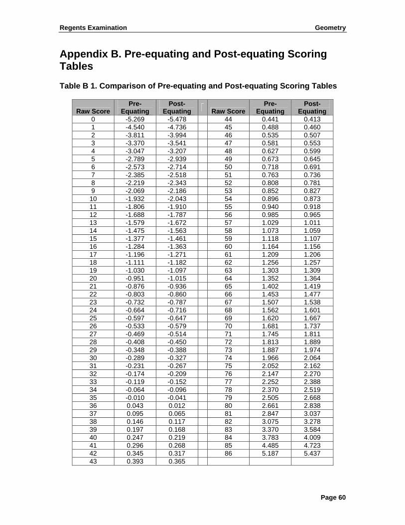
Regents Examination Geometry
Page 60
Appendix B. Pre-equating and Post-equating Scoring Tables Table B 1. Comparison of Pre-equating and Post-equating Scoring Tables
Raw Score Pre-
Equating Post-
Equating Raw Score Pre-
Equating Post-
Equating 0 -5.269 -5.478 44 0.441 0.413 1 -4.540 -4.736 45 0.488 0.460 2 -3.811 -3.994 46 0.535 0.507 3 -3.370 -3.541 47 0.581 0.553 4 -3.047 -3.207 48 0.627 0.599 5 -2.789 -2.939 49 0.673 0.645 6 -2.573 -2.714 50 0.718 0.691 7 -2.385 -2.518 51 0.763 0.736 8 -2.219 -2.343 52 0.808 0.781 9 -2.069 -2.186 53 0.852 0.827 10 -1.932 -2.043 54 0.896 0.873 11 -1.806 -1.910 55 0.940 0.918 12 -1.688 -1.787 56 0.985 0.965 13 -1.579 -1.672 57 1.029 1.011 14 -1.475 -1.563 58 1.073 1.059 15 -1.377 -1.461 59 1.118 1.107 16 -1.284 -1.363 60 1.164 1.156 17 -1.196 -1.271 61 1.209 1.206 18 -1.111 -1.182 62 1.256 1.257 19 -1.030 -1.097 63 1.303 1.309 20 -0.951 -1.015 64 1.352 1.364 21 -0.876 -0.936 65 1.402 1.419 22 -0.803 -0.860 66 1.453 1.477 23 -0.732 -0.787 67 1.507 1.538 24 -0.664 -0.716 68 1.562 1.601 25 -0.597 -0.647 69 1.620 1.667 26 -0.533 -0.579 70 1.681 1.737 27 -0.469 -0.514 71 1.745 1.811 28 -0.408 -0.450 72 1.813 1.889 29 -0.348 -0.388 73 1.887 1.974 30 -0.289 -0.327 74 1.966 2.064 31 -0.231 -0.267 75 2.052 2.162 32 -0.174 -0.209 76 2.147 2.270 33 -0.119 -0.152 77 2.252 2.388 34 -0.064 -0.096 78 2.370 2.519 35 -0.010 -0.041 79 2.505 2.668 36 0.043 0.012 80 2.661 2.838 37 0.095 0.065 81 2.847 3.037 38 0.146 0.117 82 3.075 3.278 39 0.197 0.168 83 3.370 3.584 40 0.247 0.219 84 3.783 4.009 41 0.296 0.268 85 4.485 4.723 42 0.345 0.317 86 5.187 5.437 43 0.393 0.365