new york city panel on climate change 2019 report chapter ...ann. n.y. acad. sci. issn 0077-8923...
TRANSCRIPT

Ann. N.Y. Acad. Sci. ISSN 0077-8923
ANNALS OF THE NEW YORK ACADEMY OF SCIENCESSpecial Issue: Advancing Tools and Methods for Flexible Adaptation Pathways and Science Policy IntegrationORIGINAL ARTICLE
New York City Panel on Climate Change 2019 ReportChapter 8: Indicators and Monitoring
Reginald Blake,1 Klaus Jacob,2 Gary Yohe,3 Rae Zimmerman,4 Danielle Manley,5
William Solecki,6 and Cynthia Rosenzweig7
1New York City College of Technology, City University of New York, Brooklyn, New York. 2Lamont-Doherty Earth Observatory,Columbia University, Palisades, New York. 3Wesleyan University, Middletown, Connecticut. 4Wagner Graduate School ofPublic Service, New York University, New York, New York. 5Center for Climate Systems Research, Columbia University, NewYork, New York. 6City University of New York, Hunter College, New York, New York. 7NASA Goddard Institute for SpaceStudies, New York, New York
Contents
8.1 Introduction8.2 Climate change indicators and monitoring
systems relevant to urban areas8.3 Framing the New York City Climate Change
Resilience Indicators and Monitoring System(NYCLIM)
8.4 Transportation indicators8.5 Energy indicators8.6 Infrastructure interdependency indicators8.7 Financial and economic indicators8.8 Indicators of aggregate economic health8.9 Implementation of the proposed NYCLIM
8.10 Conclusions and recommendations
8.1 Introduction
The Indicators and Monitoring chapter of the firstNew York City Panel on Climate Change Reportbegan with the paradigm: What cannot be measuredcannot be managed (Rosenzweig et al., 2010). Thisstatement is as valid today as it was then.
The NPCC1 (2010) Indicators and Monitoringchapter addressed the need for assembling a suiteof indicators to monitor climate change andadaptation in order to inform climate changedecision making. It outlined criteria for selectionof indicators (policy relevance, analytic soundness,measurability), defined categories of indicators(physical climate change; risk exposure, vulnerabil-ity, and impacts; adaptation; new research), andprovided examples of specific indicators. Table 8.1is a summary table of indicator development
contribution from the NPCC1 I&M chapter (Jacobet al., 2011). The chapter explored the institu-tional requirements for indicator data availability,continuity, archiving, and public accessibility.
NPCC2 (2015) focused on how New York City’sclimate measurement, monitoring, and assessmentactivities may be better coordinated and enhancedto guide the city in becoming more responsive toongoing climate change (Rosenzweig et al., 2015). Itlaid out a process by which a Climate Resilience Indi-cators and Monitoring System could be developedbased on the opportunities and gaps in its existingmonitoring efforts.
The combination of the climate trends presentedin NPCC1 and updated in NPCC2, the documen-tation of existing monitoring efforts, and the layingout of an indicators and monitoring developmentprocess have helped the city to advance toward arisk-oriented process for climate-oriented indica-tors and monitoring. Figure 8.1 depicts the iterativerisk management scheme for indicator selection thatis used by the NPCC. The indicator and monitoringstudies of NPCC1 and NPCC2 have made signifi-cant progress in steps 1–3 of the figure, and steps4–5 are the primary indicator and monitoring fociof NPCC3 that also provides guidance for steps 6and 7.
Steps 4 and 5 remain the primary foci of NPCC3;however, in accordance with the steps outlined inFigure 8.1, the NPCC3 I&M team has also accom-plished the following 5 of the 7 steps:
1. Interacted with New York City’s ClimateChange Adaptation Task Force (CCATF),
doi: 10.1111/nyas.14014
230 Ann. N.Y. Acad. Sci. 1439 (2019) 230–279 C© 2019 New York Academy of Sciences.
https://ntrs.nasa.gov/search.jsp?R=20190002193 2020-03-28T07:28:15+00:00Z

Blake et al. New York City Panel on Climate Change 2019 Report
Table 8.1. Basic climate change variables for monitoring and development of indicators (from NPCC1, Jacob et al.,2010)
Climate hazard Location Time series Timescale Source
Temperature Mean temperature Central Park 1876–Present Daily, monthly NCDCKennedy Airport 1948–Present Daily, monthly NCDCLaGuardia Airport 1947–Present Daily, monthly NCDC
Days with temp > X0F Central Park 1944–Present Monthly NCDCDays with temp < X0F LaGuardia Airport 1948–Present Monthly NCDCNumber of consecutive days (thresholds
preset, requires further processing tocustomize)
Central Park 1876–2001 Monthly, annual NCDC
Kennedy Airport 1949–Present Monthly NCDC1949–2001 Monthly, annual NCDC
LaGuardia Airport 1948–2001 Monthly, annual NCDCGlobal surface temperature Global value 1880–Present Annual NCDCU.S. Heat Stress Index New York City 1948–Present Annual NCDC
Precipitation Total precipitation Central Park 1876–Present Daily, monthly NCDCKennedy Airport 1949–Present Daily, monthly NCDCLaGuardia Airport 1947–Present Daily, monthly NCDC
Drought New York City Region 1900–Present Monthly NCDCThunderstorms/lightning New York County 1950–Present Daily NCDCSnow Central Park 1876–Present Daily, monthly NCDC
Kennedy Airport 1948–Present Daily, monthly NCDCLaGuardia Airport 1947–Present Daily, monthly NCDC
Downpours (precipitation rate/hour) Kennedy Airport 1949–Present Hourly NCDCLaGuardia Airport 1948–Present Hourly NCDC
Days with rainfall > x inches Central Park 1944–Present Monthly NCDCNumber of consecutive days (thresholds
preset, requires further processing tocustomize)
Central Park 1876–2001 Monthly, annual NCDC
Kennedy Airport 1949–Present Monthly NCDC1949–2001 Monthly, annual NCDC
LaGuardia Airport 1948–Present Monthly NCDC1948–2001 Monthly, annual NCDC
Sea level riseand coastalstorms
Sea level rise – mean water level the Battery 1856–Present Monthly NOS
Sandy Hook, New Jersey 1932–Present Monthly NOSHourly height water level the Battery 1958–Present Hourly NOSExtreme winds Sandy Hook, New Jersey 1910–Present Hourly NOSTropical cyclones Central Park 1900–Present Daily NCDC
New York 1851–Present Annual NCDCOther Greenhouse gas index Global value 1979–Present Annual ESRL
with New York City’s Office of Recoveryand Resiliency (ORR), with New York City’sDepartment of Transportation, and with NewYork City’s Comptroller’s office. These inter-actions were carried out via workshops, meet-ings, and teleconferences
2. Focused on the energy and transportation sec-tors because of data availability, ease of acces-sibility relative to other sectors, and time
3. Selected a set of preliminary indicators4. Presented the set of preliminary indicators to
stakeholders at CCATF meetings for feedbackand to scope implementation
5. Considered indicator revisions based on stake-holder feedback
Steps that remain include:
6. Provide guidance to the NPCC4 team in set-ting up an I&M system that reflects the definedframework
7. Provide guidance to the NPCC4 team inconducting evaluation, iterative research, andstakeholder interaction through time
Stakeholder interactions for the I&Mco-generated processIn developing the proposed New York City ClimateResilience Indicators and Monitoring (I&M) Systempresented in this chapter, a co-generation processtook place between the author team, germane
231Ann. N.Y. Acad. Sci. 1439 (2019) 230–279 C© 2019 New York Academy of Sciences.

New York City Panel on Climate Change 2019 Report Blake et al.
Figure 8.1. Iterative risk management indicator and monitoring selection process (NPCC, 2015).
stakeholders, research scientists, and climateexperts (See Appendix 8.A. for full description ofthe process). The process also included reviewingthe current literature on risk-oriented indicatorsand monitoring for climate change resiliency.
The genesis of the co-generated process is rootedin the NPCC aligning its initial broad indicatorsand monitoring framework to the five key “lifeline”infrastructure sectors (1)transportation, (2) energy,(3) telecommunications, (4) social infrastructure,and (5) the combined sector consisting of water,sewer, and waste that were identified by the NewYork City Climate Change Adaptation Task Force(CCATF).
These five sectors and their possible links to cli-mate are highlighted in Table 8.2. Some additionalpreliminary discussions, including potential brain-storming around indicators and data sources, alsooccurred between the NPCC and some CCATFmembers. These were followed by a workshop, aroundtable, and continuing discussions throughoutthe scoping and drafting process.
The primary CCATF agencies and organizationsengaged included The Metropolitan TransportationAuthority, The NYC Department of Transportation,The NYC Department of Environmental Protection,
Port Authority of New York and New Jersey, EasternGeneration, and Con Edison. Additional feedbackwas also obtained from the NYC Emergency Man-agement Office and The NYC Comptroller’s Office.
The development of the chapter included reviewof key literature by the authors and review by keystakeholders:
� Key literature. As in the case of Chapter 7,the following NPCC and government litera-ture were used: NPCC1 (2010) and NPCC2(2015); PlaNYC (City of New York, 2013);OneNYC (City of New York, 2015); the 1.5 Cel-sius Aligning NYC with the Paris Climate Agree-ment report (City of New York, 2018a); theNYC Mayor’s Office of Recovery & ResiliencyClimate Resiliency Design Guidelines (NYCMayor’s ORR, April 2018); the NYC Office ofthe Mayor Mayor’s Management Report (2017);New York State reports, particularly follow-ing Hurricane Sandy (e.g., NYS, 2013); andU.S. Department of Homeland Security (DHS)reports (U.S. DHS, 2013, 2015)
� Key stakeholders and reviewers. The NYCCCATF, The NYC Department of Transporta-tion, The NYC Mayor’s Office of Recovery &Resiliency, The NYC Emergency Management
232 Ann. N.Y. Acad. Sci. 1439 (2019) 230–279 C© 2019 New York Academy of Sciences.

Blake et al. New York City Panel on Climate Change 2019 Report
Table 8.2. Key climate extremes identified five key proposed NYCLIM sectors based on feedback and interactionswith the New York City Climate Change Adaptation Task Force
City-selected sectors Climate extremes
Transportation Sea level rise and coastal flooding; extreme heat and humidity; extreme winds
Energy Sea level rise and coastal flooding; extreme heat and humidity; cold snaps
Telecommunications Sea level rise and coastal flooding; extreme heat and humidity; extreme winds
Social infrastructure Sea level rise and coastal flooding; extreme heat and humidity; heavy rainfall/inland flooding
Water, sewer, and waste Sea level rise and coastal flooding; extreme heat and humidity; heavy rainfall/coastal flooding
Office, and The NYC Comptroller’s Office,The NYC Office of Management and Bud-get, The Metropolitan Transportation Author-ity, The NYC Department of EnvironmentalProtection, Consolidated Edison, and The PortAuthority of New York and New Jersey.
Organization of chapterThis chapter presents the work that has been under-taken by NPCC3 to advance the conceptualizationand recommendation of a proposed New York CityClimate Change Resilience Indicators and Monitor-ing System (NYCLIM). While NPCC1 and NPCC2were primarily focused on enhancing the resiliencyof critical infrastructure throughout the city andregion, NPCC3 has broadened its scope to includesocial vulnerability and economic indicators. Thechapter also presents several case studies to illus-trate the status of indicator development for theCity. Moreover, it provides a detailed set of indica-tors in the Appendix.
Section 8.2 reviews the literature on existing cli-mate change indicators and monitoring systemsso that New York City may learn from whatother cities and levels of government have done.Section 8.3 offers the framework for a proposed NewYork City Climate Change Resilience Indicators andMonitoring System (NYCLIM). Sections 8.4 and 8.5explore indicators specifically aimed, respectively, atthe transportation and the energy sectors, and Sec-tion 8.6 covers selected infrastructure interdepen-dencies for those two sectors.
Section 8.7 discusses financial and economic indi-cators, and Section 8.8 provides insights for aggre-gate economic well-being and how to measure it asa function of the potential costs of climate change.Section 8.9 discusses the implementation of the pro-posed NYCLIM, and the final Section, 8.10, pro-vides a conclusion that discusses gaps in knowledgeand/or missing data, and avenues for implementa-tion and further research.
Appendix 8.A describes the co-generation processin greater detail. Appendix 8.B offers a short intro-duction to how the steps in Figure 8.1 can reflect andincorporate a dynamic climate and its detection andactivity to human activity. An I&M system needs toaccurately account for how the future climate ofthe city might evolve over the near term (2020s),medium term (2050s), and long term (2080s, 2100,and beyond).
8.2 Climate change indicators andmonitoring systems relevant to urbanareas
This section is an illustrative listing of local, regional,national, and international contributions relevantto urban climate change indicator and monitoringsystems, such as the one being recommended inthis chapter. The creation of effective indicators forassessing vulnerability to climate change must beginwith clear understanding of the diversity of localand regional domains (Downing et al., 2001). Theyneed to be connected clearly with ranges of adapta-tion strategies and options so that they can eventu-ally identify vulnerabilities and adaptation measuresrelated to observed situations and/or their projectedfuture.
It follows that spatial and temporal scales are crit-ical dimensions for indicators regardless of contextand that consistency across contexts needs to beassured to allow at least qualitative if not quantita-tive comparisons over time and space, and to detecttrends and differences.
8.2.1 U.S. global change indicators andmonitoring
There are at least three depositories of indicatorsof climate change located within the U.S. govern-ment. They generally report historical values atvarious time scales and at various levels of geo-graphic scale, and they sometimes provide bothgraphical plots of the data and illustrative maps
233Ann. N.Y. Acad. Sci. 1439 (2019) 230–279 C© 2019 New York Academy of Sciences.

New York City Panel on Climate Change 2019 Report Blake et al.
for visual representation. Appendix 8.C recordstheir contents and electronic locations. Specificindicators that are most relevant for analyses ofurban vulnerability and resilience like NPCC3 areindicated.
Linking fundamental framework elements of themacroscale national I&M systems to New York City’sclimate resiliency indictors can be helpful in regardto the understanding of trends. By collecting, archiv-ing, and analyzing some of the same indicators at theNew York metropolitan region scale, the NYCLIMproposed in this chapter by the NPCC3 could pro-vide perspective, for instance, on whether the cli-mate trends it is experiencing are similar or differentfrom regional and national trends (Rosenzweig andSolecki, 2018).
� U.S. Environmental Protection Agency (EPA)
Historical trajectories of annual and sometimesmonthly data at national, regional, and occa-sionally local scales are provided for green-house gas and short-lived pollutant emissions,weather, and climate (temperature, precipitation,extreme events, tropical cyclones, river flood-ing, and drought), health (heat-related deaths,lyme disease and West Nile virus, growingseasons lengths), and oceans (coastal flood-ing, land loss, Arctic sea ice); see https://www.epa.gov/climate-indicators.
� National Oceanographic and AtmosphericAdministration (NOAA)
Historical trajectories of annual data at national,regional, state, and occasionally local scales areprovided for yearly climate rankings for precipi-tation, temperature, and drought; extremes (hotand cold, wet and dry); societal impacts (cropmoisture, energy demand, wind, wildfires, $1billion disasters, West Nile virus, hurricanes, tor-nadoes); and oceans (sea level rise, Arctic seaice, sea surface temperature, oscillations (ENSO,NAO, PDO, PNA)); see https://www.ncdc.noaa.gov.
� United States Global Change Research Pro-gram (USGCRP).
Historical trajectories of annual data at nationaland global scales are provided for greenhouse
gases, surface temperature, start of spring,surface temperature, and Arctic sea ice; seehttps://globalchange.gov/explore/indicators.
8.2.2. Global cities and selected New YorkCity indicators and monitoring sources
Other urban-scale compilations of I&M measureshave been developed that included New York City.Examples are summarized below, and results forboth indices are contained in Appendix 8.C.
� The National Academies (2016) produced“Pathways to Urban Sustainability: Challengesand Opportunities for the United States” thatidentified numerous climate-related indicatorsand applied them to nine cities, including NewYork City.
� The Economic Intelligence Unit (2012) as partof its Green Cities Index covered New York Cityas part of its North America study.
� Urban Climate Change Research Network(UCCRN) Second Assessment Report on Cli-mate Change and Cities (ARC3.2) through itsCase Study Docking Station (CSDS) collectsdata on a set of useful indicators for cities(Rosenzweig et al., 2018). New York City is rep-resented by several case studies in the ARC3.2CSDS.
8.3. Framing the New York City ClimateChange Resilience Indicators andMonitoring System (NYCLIM)
Figure 8.2 depicts the proposed operational com-ponents of the proposed NYCLIM. These opera-tional components include data processing centersand online repositories of climate change adapta-tion databases that are equipped with references,resources, topical categories, and key words. Addi-tionally, the proposed system includes community–stakeholder partnerships that inform decisionmakers and contribute to prudent, equitable, andscientifically sound climate change policy. The sys-tem would also be robust and flexible enough toincorporate ongoing research and new knowledge,the potential for indicators to change, and for newindicators to be developed.
Variables of a future, proposed NYCLIM shouldinclude climate extremes, social vulnerability sec-tors and their interdependencies, infrastructurevulnerability, and decision time frames. Purpose,
234 Ann. N.Y. Acad. Sci. 1439 (2019) 230–279 C© 2019 New York Academy of Sciences.

Blake et al. New York City Panel on Climate Change 2019 Report
Figure 8.2. Prototype structure and functions of the proposed New York City Climate Change Resilience Indicators andMonitoring System (NYCLIM). The proposed system tracks four types of indicators from data collection agencies, processingcenters, urban decision makers, and policies, projects, and programs. The proposed NYCLIM is co-generated by scientists, practi-tioners, and local communities to determine which indicators should be tracked over time to provide the most useful informationfor planning and preparing for climate change in New York City.
metrics, data availability, and potential challengesand/or limitations should also be suggested for eachindicator.
The selection of indicators that reflect climate,social, infrastructure, and economic variables canenable the tracking of:
1. Climate: Climate variables that portendrelated stress for human systems;
2. Impacts: Links that display how and when thatstress produces the physical and social impactsof the climate change;
3. Vulnerability: Associations that can previewvulnerabilities that are the critical manifesta-tions of climate from climate change impactinformation; and
4. Resilence: Indicators that inform andhelp decide adaptive response to promoteresilience.
For each indicator, a rationale, measurementunits, definitions, and data sources are provided.Multistep links to resiliency may be either direct orindirect, and either work alone or as part of a col-lection of amplifying drivers. In Appendix 8.D, wesystematically summarize in a matrix form how toorganize the information that could be made avail-able to define, characterize, and quantify an indica-tor and its purpose.
8.3.1. Climate extremesThe NPCC3 tracked six climate extremes that areimportant for monitoring climate change (seeChapters 2, 3, and 4). They are extreme heat andhumidity, heavy downpours, drought, sea level
rise and coastal flooding, extreme winds, and coldsnaps. A robust set of climate indicators enablesthe quantification of trends and importantlythe juxtaposition of these trends with climateprojections. Table 8.3 highlights such an examplefor temperature (see Chapter 2, Climate Science).
To analyze where current temperature trendsfall within the NPCC2 projections for the 2020s,monthly temperature data (1971–2017) from theCentral Park, New York weather station were ana-lyzed (Table 8.3). For the annual average and thewinter (DJF) and summer (JJA) seasonal averages,the linear trend in temperature change was com-puted. The rate of warming per year was multi-plied by the number of years in the observed period.This amount of warming was then compared to theranges of projections from the NPCC2 report.
For the annual and summer warming, observedincreases in temperature fall below the 10thpercentile projection value. For the winter, theobserved warming falls within the middle range ofprojections.
As a caveat, it is important to note that while theobservations (based on the linear warming trend)fall within the lower end of the projections, themost appropriate comparison, which would take theobserved future period and subtract the observedbase period, cannot be computed as the future win-dow is too short and the average would be domi-nated by year-to-year variability. On a related note,some indicators may track how climate projectionsthemselves change as climate science and observa-tions progress.
235Ann. N.Y. Acad. Sci. 1439 (2019) 230–279 C© 2019 New York Academy of Sciences.

New York City Panel on Climate Change 2019 Report Blake et al.
Table 8.3. Comparison of climate trends from 1971 to 2017 compared to NPCC2 projections for the 2020s
2020s NPCC2
projections—low estimate
2020s NPCC2
projections—middle range
2020s NPCC2
projections—high estimateLinear warming trend
(1971–2017) (10th percentile) (25th–75th percentile) (90th percentile)
Annual 1.43°F 1.5°F 2.0°F–2.9°F 3.2°F
Winter (DJF) 2.42°F 1.4°F 2.0°F–3.2°F 3.7°F
Summer (JJA) 0.55°F 1.8°F 2.1°F–3.1°F 3.3°F
Note: These comparisons should be viewed with caution because of the role that natural variation plays in the short term.
8.3.2. Social vulnerabilityNPCC3 has a major focus on social vulnerability(see Chapter 6, Community-Based Assessments).Chapter 6 includes a detailed description of socialvulnerability indicators.
8.3.3. SectorsWith inputs from ORR and from the CCATF andthe agencies that comprise it, NPCC3 selected fivesectors (Fig. 8.3) related to critical infrastructure—energy, transportation, telecommunications, trans-portation, and water, waste, and sewers. Throughstakeholder interactions, the NYCLIM proposedhere identifies the major climate-related risks foreach sector exemplified by heat in Table 8.3. Dueto data availability, ease of data accessibility, andtime constraints, this chapter only focuses on theenergy and transportation sectors. The underlyingpentagon of the five sectors of Figure 8.3 drawsattention to interdependencies across the sectors,both in terms of their functional interconnectionsand in terms of the climate variables that may drivemultiple impacts and vulnerabilities.
8.3.4. Infrastructure vulnerability, impacts,and resilience
Indicators will enable the comparison of past,present, and future vulnerabilities, impacts, andultimately resilience. For example, these indica-tors relate to the management of climate impacts.Their purpose is to track whether climate adap-tation policies and measures are gaining or los-ing ground to manage the risks to which the city,its population, assets, infrastructure, and econ-omy are exposed. This set of indicators focusedon infrastructure is aimed to provide a soundquantitative database that can help the city tomake decisions on relevant policies, planning andfunding priorities, and to allow the city to opti-mally manage its social, economic, and fiscal health
vis-a-vis climate challenges encompassing a risk-oriented framework.
8.3.5. Decision-making time horizonsAn indicator can address multiple time horizons.For the physical climate indicators, the time hori-zons directly rely on the projections in Chapter 2,New Methods for Assessing Extreme Temperatures,Heavy Downpours, and Drought; Chapter 3, SeaLevel Rise; and Chapter 4, Coastal Flooding. Theseare the 2020s, 2050s, 2080s, and the year 2100. Forindicators and time frame of social vulnerability, seeChapter 6, and for the risk time frames of criticalinfrastructure, see Chapter 7, Critical Infrastruc-tures. Certain infrastructure systems such as trans-portation, rights of way, bridges, and tunnels may,in some instances, have expected useful life timesbeyond the upper time limit (2100) for which Chap-ters 2, 3, and 4 provide climate projections.
We distinguish broadly three time horizons forthe risk-related indicators: short term (ST) throughthe 2020s (2010–2039 time frame), medium term(MT) in the 2050s (2040–2069 time frame), andlong term (LT) in the 2080s (2070–2099 time frame),2100, and beyond. These horizons dovetail approxi-mately to the climate science time slices of the 2020s(ST), 2050s (MT), and 2080s–2100 (LT) (see Chap-ters 2, 3, and 4). The boundaries between the timehorizons are left imprecise to reflect a degree ofuncertainty in their distinction from one applica-tion to another.
Details in our constructions are recorded inAppendix 8.E. The chapter looks forward, as deci-sion makers do, from the immediate term intouncertain climate futures. A key question is: Canwe describe climate futures in decadal steps so thatthe essential short-, medium-, and long-term con-texts can be rigorously distinguished in ways thatare consistent with the 2100 distributions? Box 8.1
236 Ann. N.Y. Acad. Sci. 1439 (2019) 230–279 C© 2019 New York Academy of Sciences.

Blake et al. New York City Panel on Climate Change 2019 Report
Figure 8.3. Five city-selected lifeline infrastructure sectors.
explores how this challenge is being addressed inMiami Beach.
8.4. Transportation indicators
Extreme heat and humidity, cold snaps, heavydownpours, extreme winds, sea level rise, andcoastal flooding are increasing in frequency andintensity (see Chapters 2, 3, and 4), posing majorhazards that produce climate-related risk for the
transportation sector. Key indicators can track thesechanges, their impacts on New York City trans-portation infrastructure, and even highlight changesin vulnerability and resiliency of that system overtime. Potential indicators related to transportationand their associated purpose, definitions, metrics,time frames, and data sources are summarized inTable 8.4. Background information on climate issues
Box 8.1. The time horizon challenge: responding to flooding in Miami Beach
Miami Beach has experienced a 400% increase in tidal flooding since 2006. The city understood that craftingindicators to monitor changes in sea level rise and associated flooding risk as well as changes in social andeconomic vulnerability was essential to building some pre-emptive skill into risk management programs andpolicies, even back to the immediate time frame. Miami Beach is now in the midst of a $400 million project toraise roads and install new sewers and pumping stations. This project was initially designed to hedge againstthe upper tails of sea level rise futures, and the city was committed to monitoring the oceans to see when thenew infrastructure might be overwhelmed. However, actual adaptations were designed to just deal withincreased nuisance flooding while at the same time allowing more development. The adaptations are unlikelyto be effective in the long run, given current sea level rise projections. Planners, therefore, face a complicatedquestion: What indicator could be constructed to properly characterize current adaptation investments thatmay encourage additional real-estate development, vis-a-vis the adaptation investments’ long-term efficacy,sustainability, or lack thereof?
Sources: Wdowinski et al., 2016; Miami New Times, 2016; and NPR, 2016.
237Ann. N.Y. Acad. Sci. 1439 (2019) 230–279 C© 2019 New York Academy of Sciences.

New York City Panel on Climate Change 2019 Report Blake et al.
Table 8.4. Illustrative and potential climate-linked critical indicators for selected climate extremes for New YorkCity’s transportation sector (road and rail systems only)—impacts, indicators, metrics, and data sources
Climate
extremesaPotential infrastructure
impactsb Potential indicatorsc Potential indicator metricscGeneral illustrative and
potential data sources
Extreme heat
and humidity
Roadd
– Increased road material
degradation, result-
ing in increased road
maintenance
1. Distortion including buckling of
road surfaces
2. Number, frequency, and cost of
repairs
3. Emergency safety alerts, etc.
4. Working days of pavement crews
(attributable to both climate and
non-climate factors)
1. Extent (e.g., area) of roadway seg-
ments requiring repair
2. Cost in dollars of roadway repair over
time, considering changes in labor
and material costs
3. Number and duration of activations
4. Number and cost of changes in work
day allocations (attributable to both
climate and non-climate factors)
1. NYC DOT, NYS DOT,
PANYNJ
2. NYC DOT, NYS DOT,
PANYNJ
3. NYCEM
4. NYC DOT, NYS DOT,
PANYNJ
Raild
– Increased heat stress on
rail equipment
1. Distortion including buckling of
rail lines and rail connectors
1. Number and mileage of rail lines
buckling; change in zero thermal
stress temperature (which can be con-
sidered a baseline in terms of temper-
ature at which running rail is neutral/
unstressed)
1. NYS MTA/NYC Tran-
sit; PANYNJ
– Increased use of cool-
ing equipment due to
increased underground
station temperatures
1. Increased use of cooling equip-
ment: frequency of use
2. Disruptive fires
3. Emergency alert activations
1. Cost of increased cooling
2. Number and intensity of disruptive
fires
3. Number and duration of safety alerts
1. NYS MTA/NYC Tran-
sit; PANYNJ
2. NYS MTA/NYC Tran-
sit; PANYNJ
3. NYS MTA/NYC Tran-
sit; PANYNJ; NYC EM
– Increased rail degradation
and equipment deteriora-
tion, resulting in increased
maintenance
1. Subway on-time performance
2. Working days of rail crews
(attributable to both climate and
non-climate factors)
1. Yearly average, but sampled every day,
if possible to allow correlation with
extreme heat, and for each subway
line
2. Number, frequency, and costs of
rail components and labor costs
(attributable to both climate and
non-climate factors)
1. NYS MTA/NYC Tran-
sit; PANYNJ
2. NYS MTA/NYC Tran-
sit; PANYNJ
– For rail systems depen-
dent on overhead catenar-
ies (or cables) for power,
for example, commuter
rail, potential increase
in transit accidents from
train collisions with sag-
ging overhead lines
1. Delays due to transit conditions
2. Health effects on passengers and
workers
1. Number, types, and duration of
delays
2. Number and severity of medical
emergencies
1. NYS MTA/NYC Tran-
sit; PANYNJ
2. NYS MTA/NYC Tran-
sit; PANYNJ, NYCEM
– Decreased service and/or
lack of service
1. Number and duration of service
disruptions (weather related) in
terms of customer wait time
2. 311 complaints
1. Customer wait time; length of trips
2. Frequency and volume of 311 com-
plaints
1. NYS MTA/NYC Tran-
sit; PANYNJ
2. NYC EM; NYC311
Cold snaps Roadd
– Some road surfaces could
be damaged depending on
material tolerances
1. Road surface disruptions, block-
ages, congestion
1.a Number, frequency, and duration of ser-
vice disruptions; trip delay time
1.b Miles and area of roadways and access
points affected
1.a NYS DOT, NYC DOT
1.b NYS DOT, NYC DOT
– Increased use of snow and
ice removal, where snow
and icing accompany cold
snaps
1. Deployment of Department
of Sanitation (DSNY) salt/sand
trucks
1. Number of trucks deployed to clear
roads and area of roadways affected
1. NYC DOT, DSNY
Raild
– Service disruption 1. Subway on-time performance
2. Decreased service and/or lack of
service; customer wait time
1. Yearly average, but sampled every day,
if possible to allow correlation with
extreme cold temperatures, and for
each subway line
2. Number and duration of service dis-
ruptions; trip delay time
1. NYS MTA/NYC Tran-
sit; PANYNJ
2. NYS MTA/NYC Tran-
sit; PANYNJ
Continued
238 Ann. N.Y. Acad. Sci. 1439 (2019) 230–279 C© 2019 New York Academy of Sciences.

Blake et al. New York City Panel on Climate Change 2019 Report
Table 8.4. Continued
Climate
extremesaPotential infrastructure
impactsb Potential indicatorsc Potential indicator metricscGeneral illustrative and
potential data sources
Cold snaps Roadd
– Increased use of snow and
ice removal, where snow
and icing accompany cold
snaps
1. Deployment of DSNY salt/sand
trucks
2. Working days of outdoor MTA
crews
1. Number of trucks and other spe-
cialized snow clearance equipment
deployed to clear rail lines and length
of rail affected
2. Number of extra days and costs per
day
1. NYS MTA/NYC Tran-
sit; PANYNJ; DSNY;
railroad owners and
operators
2. NYS MTA/NYC Tran-
sit; PANYNJ; NYC-
DOS
– Some rail components
could be damaged
depending on material
tolerances
1. Increased maintenance
2. Working days of outdoor MTA
crews
1. Number and costs of repairs
2. Number of extra days and costs per
day
1. NYS MTA/NYC Tran-
sit; PANYNJ; NYC-
DOS
2. NYS MTA/NYC Tran-
sit; PANYNJ; NYC-
DOS
Sea level rise and
coastal
flooding
Roadd
– Declining serviceability of
roadways due to flooding
conditions
1. Road obstructions and
restrictions
1. Number of storm-flood-related clo-
sures of major road arteries, for
example, Belt Parkway and/or West-
Side and/or FDR Highways
1. NYSDOT, NYC DOT
– Increased travel delay
from increased conges-
tion due to persistent high
water levels
1. Road-related closures, such as
ramps and tunnels
2. Overall road service condition
1. Number of road closures/year
2. Level of service (LOS) based on vol-
ume to capacity ratios and extent of
roads at or exceeding LOS E and F
1. NYSDOT, NYC DOT
2. NYSDOT, NYC DOT
– Increased need for ongo-
ing pumping capacity
and associated increased
energy use for additional
pumping to continuously
remove excess water to
prevent flooding
1. Road-related closures, such as
ramps and tunnels
2. Energy use for pumping opera-
tions
1. Number and duration of road clo-
sures/year
2. Marginal increase in energy use in
kWh
1. NYS DOT
2. NYS DOT,
3. ; Con Edison
– Increased use of barri-
ers and road hardening to
prevent erosion and over-
topping
1. Bulkhead/street end hardening 1. Number and cost of construction of
hardening structures
1. NYSDOT, NYC DOT
– Deterioration (corrosion)
of roadway support facili-
ties by salt water
1. Signal, CCTV, and street light
disruptions
1. Frequency of water intrusion into
electrical systems and conduits,
degree of damage, and outages
1. NYS DOT, NYC DOT;
NYC DEP
Raild
– Increased rail degrada-
tion and equipment dete-
rioration from saltwater
inundation, resulting in
increased maintenance
1. Train arrival/ departure delays
2. Flooding, debris damages, cor-
rosion, water intrusion
3. Equipment damage and repair
costs
1. Mean distance between failures for
trains; signal and switch malfunction
frequency (to the extent that other
non-climate factors do not override
climate effects); Number and fre-
quency of alerts, for example, MTA
service alerts
2. Volume of debris accumulation
3. a. Capital versus operations cost
changes
b. Equipment retrofit needs: number
and cost of relocating equipment
c. The number of protected or flood-
proofed subway entrances, given at
the end of each calendar year, in the
1%/year flood zone or other spec-
ified flood zones, compared to the
total number of subway entrances
in this zone
1. NYS MTA/NYC
Transit
2. NYS MTA/NYC
Transit
3. NYS MTA/NYC
Transit
– Service disruptions 1. Subway on-time performance
2. Rail tunnel, track, and station
closures
3. Effects of environmental haz-
ards on services
1. Number and duration of service dis-
ruptions; on-time performance rates
2. Number and duration of closures
3. Extent and severity of environmental
and public safety hazards
1. NYS MTA/NYC
Transit
2. NYS MTA/NYC
Transit
3. NYS MTA/NYC
Transit
Continued
239Ann. N.Y. Acad. Sci. 1439 (2019) 230–279 C© 2019 New York Academy of Sciences.

New York City Panel on Climate Change 2019 Report Blake et al.
Table 8.4. Continued
aClimate extremes in Table 8.4 related to transportation are as defined in NPCC3 as follows:Extreme heat and humidity pertains to heat waves as described in Chapter 2, using the National Weather Service (NWS) definition“as three (or more) consecutive days with temperatures of at least 90°F (32.22°C)” and also considers days per year above 90°F and100ᵒF. Other concepts include worst daily heat–humidity combination “wet-bulb” temperature per year; Heat index: 2-consecutivedays of heat index 80–105°F; Monthly and yearly degree cooling days for NYC (NYS ISO, 2017a zone J). Chapter 2 also developsdefinitions for heat wave frequency, duration, and intensity all of which potentially affect infrastructure.Cold snaps are defined as number of days below a threshold temperature and is reflected in the number of cooling days.Sea level rise and coastal flooding is defined in Chapters 3 and 4.bPotential infrastructure impacts and the references for each of the impacts are in general from the third column of Table 7.1b (seeChapter 7), with a few differences, in order to consistently link impacts to indicators and metrics. The end of Table 7.1 providesreferences for impacts listed in Table 8.4 as well. As indicated in footnote c for Table 7.1b, the impacts listed here are illustrative and arenot intended to be comprehensive. Non-climate–related factors in addition to climate extremes can contribute to impacts, indicatorsand indicator metrics listed here. More knowledge and analysis would be required to separate climate and non-climate factors. Theindicators are thus labeled “potential” for consideration and review by relevant agencies. Sources that underscore this selection andalso provide additional information for each impact are located in footnote (d) below.cMetrics apply to each indicator associated with each impact (in a given row) even where multiple indicators and metrics are listed.References for indicators, metrics are contained in the chapter text and references here and in Chapter 7. For detailed references notrepeated here see those accompanying Table 7.1b.dFor additional examples and details for potential climate-related transportation impacts and indicators, see, for example:For the U.S.: U.S. DOT, FHWA, Office of Planning, Environment, & Realty (HEP). 2015. Tools. Climate change adaptation. Sensitivitymatrix. https://www.fhwa.dot.gov/environment/sustainability/resilience/tools/.U.S. DOT, FHWA, Office of Planning, Environment, & Realty (HEP). 2015. Tools. Climate change adaptation. Sensitivity matrix.https://www.fhwa.dot.gov/environment/sustainability/resilience/tools/.National Academies, National Research Board, Transportation Research Board. 2008. Potential impacts of climate change on U.S.transportation. Washington, DC.http://onlinepubs.trb.org/onlinepubs/sr/sr290.pdf.U.S. Climate Change Science Program. 2008. Impacts of climate change and variability on transportation systems and infrastructure:Gulf Coast study, phase I. Synthesis and Assessment Product 4.7. https://www.globalchange.gov/browse/reports/sap-47-impacts-climate-change-and-variability-transportation-systems-andFor New York State and New York City: Various analyses and planning efforts in connection with the aftermath of Hurricane Sandycited in Chapter 7 (e.g., the NYS 2100 Commission, City of NY SIRR, etc.)Rosenzweig, C., W. Solecki, A. DeGaetano, et al. Eds. 2011. Responding to climate change in New York State: the ClimAID integratedassessment for effective climate change adaptation. Technical Report. New York State Energy Research and Development Authority,NYSERDA, Albany, NY. www.nyserda.ny.gov.
related to the transportation sector was presented inChapter 7.
Table 8.4 refers to the portion of the transporta-tion sector that focuses on rail and roads, and doesnot include marine or air transportation or otherroad-related structures such as bridges, for exam-ple. Indicators and metrics are illustrative only. Theyemphasize physical infrastructure measures and cer-tain aspects of social impact but generally not thosethat are health or safety related (see Chapter 6,Community-Based Assessments of Adaptation andEquity). Nonclimate-related factors in addition toclimate extremes can contribute to impacts, indica-tors, and indicator metrics listed here. The impacts,indicators, and metrics are thus labeled “potential”for consideration and review by relevant agencies.
Potential data sources listed are only some ofthe major organizations that provide some of the
data sources through publicly available documentsor organizations. These organizations do not nec-essarily currently use the indicators. Data sourcesacross most of the indicators and metrics for railtransit include but are not limited to: U.S. DOT, FTA,NYS MTA and MTA NYC Transit, the Port Author-ity of NY and NJ (PANYNJ), NY MetropolitanTransportation Council (NYMTC), NJ Transit andAmtrak as relevant to rail transit; NYC ORR; NYCDepartment of Sanitation (DSNY) for debris andtrash removal as relevant; for emergency functions,NYC Office of Emergency Management (NYCEM).Data sources for roadways include but are not lim-ited to: U.S. DOT, NYS DOT, NYS DOT, NYC EDC,and PANYNJ.
Not all of these agencies are listed in the datasource column. Data sources apply to each indicatorand metric listed for a given impact (in a given row).
240 Ann. N.Y. Acad. Sci. 1439 (2019) 230–279 C© 2019 New York Academy of Sciences.

Blake et al. New York City Panel on Climate Change 2019 Report
Data availability is subject to release by the agencies.The listing of data sources in this table indicatesonly that relevant data may be available. It does notindicate ability or willingness of source entity toshare information.
Many sources of historical records of variouslengths and geographical scales are available to pro-vide the basis for climate indicators, but not allof them would work at citywide and/or larger orsmaller scales (See Appendices 8.C.1 and 8.C.2).
Scope and data sourcesThe transportation sector addressed here focusesonly on rail and roads. Some transportation indica-tors that potentially can be related to climate changeexist for example for the New York City transit sys-tems from the MTA performance indicator database(MTA undated web site), for streets and bridgesfrom the NYC Mayor’s Management Report (NYCOffice of the Mayor, 2017), and for national-scalebridge indicators applicable to the city from theU.S. National Bridge Inspection Program and thestandards upon which it is based (U.S. DOT, FHWAhttps://www.fhwa.dot.gov/bridge/nbis.cfm) andthe National Bridge Inventory Program (U.S. DOT,FHWA https://catalog.data.gov/dataset/national-bridge-inventory-system-nbi-1992-b9105).
Time framesOnce these data sources have been assessed for usein the proposed NYCLIM (Section 8.9), the nextstep will be to assess the potential for finding or cre-ating forward-looking indicators for the mediumand long terms that are anchored on the mostrecent short-term end-points of the existing his-torical series.
Three time periods are used: short-term,medium-term and long-term time periods (seeAppendix 8.E for detailed discussion on timeperiods). For example, climate-related impacts ontransportation expressed in terms of indicatorsover time given in Table 8.4 include:
� In the short term (2020s), temperature-relatedimpacts and flooding could lead to disrup-tions of road and rail infrastructure (e.g., track,roads, signals, switches, lighting, and powersystems). These could be intermittent depend-ing upon the length of the impacts; however,regardless of the time period, once the equip-ment is disabled, repairs will have to be made.
� In the medium term (2050s), the impact iden-tified in the short term could persist into themedium term, should the risk factors persist.
� In the long term (2080s, 2100, and beyond),major dislocations of transportation infras-tructure and population could occur, shouldthe impacts persist over long periods of time.
ExamplesAn example of a set of simple transportation-relatedvulnerability indicators is related to the number ofnuisance flooding of low points on the FDR Drivealong the East River in Manhattan, of the West SideHighway (WSHW) along the Hudson River, and ofthe Belt Parkway in Brooklyn and Queens. Such nui-sance flood data and impacts on NYC transporta-tion could potentially be provided by the NYC DOT(or other city agencies, like NYCDEP), or could beinferred from or linked to tide gauge readings at theBattery in Manhattan when they exceed a certainthreshold value known to be associated with suchnuisance flooding.
These indicators of transportation system dis-ruption from nuisance flooding could contributeto decision making regarding whether city agenciesclose traffic on the major arteries near the coastin anticipation of surge and flood forecasts (suchas provided by NOAA’s NHC, NWS, or SIT; forsources, see footnote).
Another important measure to track is the buck-ling of rail lines from persistent heat waves. The FTAestimates that the buckling of rail lines will increasewith increasing 90-degree days (FTA, 2011). TheNew York area is not in the highest area for heat butthe amount estimated for number of days exceeding90°F is still in the range of 40–60 more days.
8.4.1 Case study 1: Transportation, sea levelrise, and coastal flooding
Inundation of a large part of the New York Citysubway system was one of the most consequentialimpacts of Hurricane Sandy (Fig. 8.4). The NationalClimate Assessment reported that “The nation’sbusiest subway system sustained the worst damagein its 108 years of operation on October 29, 2012, asa result of Hurricane Sandy” (NCA, 2014). Millionsof people were left without service for at least 1 weekafter the storm, as the Metropolitan TransportationAuthority rapidly worked to repair extensive flooddamage. It follows that developing indicators for
241Ann. N.Y. Acad. Sci. 1439 (2019) 230–279 C© 2019 New York Academy of Sciences.

New York City Panel on Climate Change 2019 Report Blake et al.
Figure 8.4. Hurricane Sandy causes flooding in New YorkCity’s subway (86th Street Lexington Ave. Station, UpperEast Side in Manhattan). Source: https://www.pinterest.com/pin/218143175672242767/.
the flood hazards across the subway system wouldbe a good idea, that is, indicators of the vulnera-bility of the system to flood hazards and how theymight change over time as the climate and the cityevolve. These indicators may include either direct orindirect estimates of how far into the future imple-mented adaption measures can be expected to beeffective.
The experience of NYC during Hurricane Sandysuggests a general indicator whose purpose, calibra-tion, and data can be characterized as:
1. Indicator. Direct flood risk/resilience of theNew York City Transit (NYCT) subway sys-tem.
2. Purpose. To measure the vulnerability of thesubway system and to keep track on a yearlybasis of adaptive measures so that decisionmakers will know whether and/or how fast thesystem’s resilience is increasing, being main-tained, or—in the face of continued sea levelrise and storms—deteriorating.
3. Metrics. On an annual basis, the number ofprotected or flood-proofed subway entrancesand other openings in the 1%/year flood zone,or at and below elevations with a specified free-board above the 1%/year base flood elevation(BFE) can be quantified. The 2015 Prelimi-nary Flood Insurance Rate Map has indicatedthe total number of subway entrances in this
zone, or at and below the specified elevationincluding freeboard.
4. Data Sources. (1) FEMA and/or ORR for1%/year flood zone maps with their BFEs(in feet), referenced to a vertical datum,for example, NAVD88; (2) NYCT for list ofprotected/flood proofed subway entrances in1%/y zone including freeboard, or at or belowa defined retrofit target elevation, and of totalnumber of entrances in the so-defined floodzone.
DiscussionThere are, however, challenges and potential prob-lems that should be explored. For example, FEMAflood zone maps can change over time, eitherbecause of changes in methodology, or because ofthe climate, including storm statistics and sea levelrise, and they require periodic updates related tothe frequency of flooding. Even now, there is uncer-tainty which 1%/year flood zone maps and relatedBFEs to use: those generated by FEMA before Sandy,or those proposed by FEMA since.
The Direct Flood Risk/Resilience indicator pro-vides a measure of resilience based on the 1%/yearprobability level. It does not provide informationabout what resilience the system has against lessprobable but more severe flood events, for example,those based on 0.2%/year or even lower probabili-ties, or those amplified by future sea level rise. Thelatter depend on future SLR rates for given futuretime horizons. This could be partly remedied byreporting the number of subway stations binned in1-foot increments of their protection levels abovethe 1%/year FEMA BFEs. This would rely on thewillingness and ability of the operating stakeholderto provide this more detailed information.
Flood-proofing subway entrances does not implythat the entire subway system is resilient. Switchesand signals are also weak points. Subway mainte-nance yards are another point of vulnerability. Ven-tilation grates (often at or near street or sidewalklevels) must be flood-proofed, as well as ventilationshafts. Additionally, other system components suchas electric power supply, communications, and con-trol systems must all be protected at the same prob-ability level, if not beyond, to make the system fullyresilient. It follows that this single, specific sampleindicator is more a proxy for resilience awarenessof the operating agency—a first step to the ultimate
242 Ann. N.Y. Acad. Sci. 1439 (2019) 230–279 C© 2019 New York Academy of Sciences.

Blake et al. New York City Panel on Climate Change 2019 Report
goal of defining more specific measures of systemresiliency.
Several suggestions for improvement of the DirectFlood Risk/Resilience indicator come to mind. Anygiven subway station is generally served by multipleentrances (e.g., in Manhattan, these are often sepa-rate for uptown and downtown directions). There-fore, an alternative indicator may be the number ofprotected/flood-proved subway stations rather thanentrances. Another option is even broader: the num-ber of completely protected subway lines. That levelof aggregation, though, presents its own difficul-ties because line designations and routing can varybetween weekdays and weekends, or even across thehours of the day, repair interruptions, or long-termconstruction projects. For details of NYCT’s currentsubway flood risk reduction program, see Box 8.2
8.5. Energy indicators
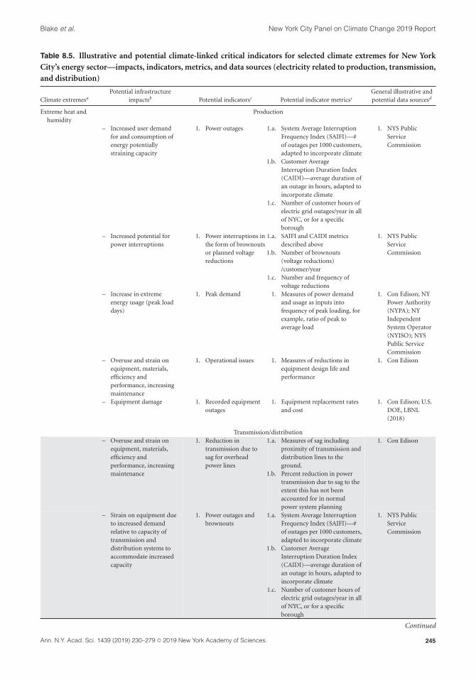
Heat waves/extreme heat, cold snaps, and coastalflooding and sea level rise are increasing in fre-quency and intensity (see Chapters 2–4), and otherextreme weather events have also been identified asmajor hazards that produce climate-related risk forthe energy sector. The purpose, definitions, met-rics, time frames, and data sources characterized aresummarized in this section (see Table 8.5). Back-ground information on climate issues related to theenergy sector was presented in Chapter 7.
Table 8.5 refers to the portion of the energy sec-tor that focuses on electricity. Energy supply in theform of fuel and its related infrastructure is notincluded here. Indicators and metrics are illustrativeonly. They emphasize physical infrastructure mea-sures and certain aspects of social impact but gener-ally do not include health- or safety-related impacts(see Chapter 6, Community-Based Assessments ofAdaptation and Equity). Non-climate–related fac-tors in addition to climate extremes can contributeto impacts, indicators, and indicator metrics listedhere. The impacts, indicators, and metrics are thuslabeled “potential” for consideration and review byrelevant agencies.
Potential data sources listed are only some ofthe major organizations that provided some ofthe data sources through publicly available docu-ments or organizations who could potentially usethe information. These organizations do not nec-essarily currently use the indicators. Data sourcesacross most of the indicators and metrics for energy
are Con Edison, the Long Island Power Authority,National Grid, the NYS Public Service Commission,NYSERDA, the NYS Independent System Operator(ISO), and a number of the electric power ownersand operators of generating facilities. Not all of theseorganizations are listed in the data source column.Data availability is subject to release by the agencies.The listing of data sources in this table indicates onlythat relevant data may be there. It does not indi-cate ability or willingness of source entity to shareinformation.
As in the discussion of transportation indicatorsabove, many sources of historical records of vari-ous lengths and geographical scales are available toprovide the basis for indicators, but not all of themwould work at citywide and/or larger or smallerscales (see Appendices 8.C.1 and 8.C.2). Many ofthe historical records selected for the transporta-tion indicators will also likely be appropriate forenergy-specific hazards. As with the transportationindicators, assessment of existing data sources is thefirst step, followed by finding or creating forward-looking indicators for the medium and long terms.
Indicators and data sourcesPotential energy reliability indicators include:
� System Average Interruption Duration Index(SAIDI) is commonly used as a reliability indi-cator by electric power utilities. SAIDI is theaverage outage duration for each customerserved (U.S. DOE PNNL, 2016: A.13)
� System Average Interruption Frequency Index(SAIFI) or the average number of interruptionsthat a customer would experience (U.S. DOEPNNL, 2016: A.13).
These indicators are not very sensitive to extremeclimate events. Hence, other indicators and reli-able data sources will be sought to characterizethe vulnerability or resiliency of electric services toextreme climate events. Cooperation with the NYSPSC and/or NYC EM needs to be pursued.
In early 2000, Con Edison developed the Net-work Reliability Index (NRI) model to evaluatethe reliability of its underground low-voltage net-work system. The program simulates failures usingthe Monte–Carlo method and runs long-range(20 years) simulations to determine the NRI valuesfor various design configurations and under vary-ing conditions including heat waves. Con Edison is
243Ann. N.Y. Acad. Sci. 1439 (2019) 230–279 C© 2019 New York Academy of Sciences.

New York City Panel on Climate Change 2019 Report Blake et al.
Box 8.2. The Metropolitan Transportation Authority and the level of tolerable risk
On October 29, 2012 Hurricane Sandy flooded a significant portion of the MTA’s New York City subwaysystem. A study produced only a year earlier had analyzed such flooding for a generic 100-year storm (Jacobet al., 2011). The MTA’s New York City Transit (NYCT) division used this information to prepare for the stormoperationally, including the removal of critical signal and control systems in many of the tunnels forecast to beflooded, in order to prevent these systems from being exposed to corrosion by brackish flood waters. Thismeasure shortened the downtime of most of the subway system from a forecasted 3–4 weeks to 1 week.
A large portion of the economy comes to a virtual halt without a functioning subway. However, long-termstructural damage to many tunnels, including those traversing the East River that connect Manhattan withBrooklyn and Queens, has required full-time or weekend closures to repair in subsequent years, causing longercommutes for many New Yorkers having to use alternate routes. The post-Sandy tunnel and station repairprogram is ongoing in 2017 and beyond, at a total cost of many billions of dollars.
From the experience of Hurricane Sandy, and the NPCC’s climate and sea level rise forecasts, it was clearthat the risk exposure for the MTA and its impact on NYC’s economy is high. The vulnerability of its varioustransportation systems, and of the subway in particular, to repeated, increasingly more frequent and severestorm flooding is clear. Hence, the MTA opted to devote a major portion of its current and future capitalprograms to reduce its flood risk exposure.
The NYCT began an inventory of openings into the belowground system that are at elevations low enoughto be at risk of flooding. Because NYC and FEMA were in the process of developing new flood zone maps forthe 1%/year flood (the “100-year flood”), related new base flood elevations (BFE), and a 0.2%/year flood map(“500-year flood”) with its higher flood elevations recommended for critical assets, the NYCT decided not towait for this mapping process to be completed.
After considerable evaluation of risks, costs, and benefits, it decided to adopt the NOAA SLOSHcomputations for storm surge elevations for a Saffir Simpson Category 2 hurricane, or more specifically itsMOMS (maximum of maximum elevation for hundreds of simulations of artificial category-2 storm tracks),and then added 3 feet on top of the SLOSH Category-2 MOMS to account for sea level rise. Three feet, or36 inches of sea level rise corresponds to a time horizon up to about the 2080s at the NPCC mid-range(25–75th percentile) SLR forecast, and to about the late 2050s for the NPCC high estimate (90th percentile)SLR forecast. This design level results, for instance, in a design elevation of 19 ft NAVD 1988 at the Battery inLower Manhattan. In 2012, Sandy crested there at about 11.3 ft NAVD 1988. Hence, this choice is likely toprovide considerable safety for about half a century, if the engineered protective measures perform as intended.
At this flood design elevation (Cat 2 + 3 ft), the NYCT has aimed at retrofitting a total of more than 3600openings ranging from subway entrances, ventilation shafts, side walk level ventilation grates, manholes andothers with about a dozen different engineered cover designs, some closing automatically and others needingprestorm deployment or activation by teams of workers to seal the openings, and elevation of grates.____________________________________________This information was compiled from the following sources:MTA. 2017. MTA climate adaptation task force resiliency report.Accessed January 28, 2019. http://web.mta.info/sustainability/pdf/ResiliencyReport.pdf
Miura, Y. et al., 2017. Vulnerabilities in New York City subway system to sea level rise and flooding.Unpublished Report for the MTA, prepared by the Columbia University Climate Change Adaptation Team(CCCART). Department of Civil Engineering, under supervision of Prof. G. Deodatis and K.H. Jacob.16 pages, 8 figures, 5 tables. Columbia University 2017.
U.S. Department of Transportation (2018). As of December 2018, the MTA has posted a total of about$ 4.55 Billion in both Sandy recovery and resiliency capital investments combined, obtained from federal funds.Accessed January 28, 2019. https://www.transit.dot.gov/funding/grant-programs/emergency-relief-program/fta-funding-allocations-hurricane-sandy-recovery-and
244 Ann. N.Y. Acad. Sci. 1439 (2019) 230–279 C© 2019 New York Academy of Sciences.
Blake et al. New York City Panel on Climate Change 2019 Report
Table 8.5. Illustrative and potential climate-linked critical indicators for selected climate extremes for New YorkCity’s energy sector—impacts, indicators, metrics, and data sources (electricity related to production, transmission,and distribution)
Climate extremesaPotential infrastructure
impactsb Potential indicatorsc Potential indicator metricscGeneral illustrative andpotential data sourcesd
Extreme heat andhumidity
Production
– Increased user demandfor and consumption ofenergy potentiallystraining capacity
1. Power outages 1.a. System Average InterruptionFrequency Index (SAIFI)—#of outages per 1000 customers,adapted to incorporate climate
1.b. Customer AverageInterruption Duration Index(CAIDI)—average duration ofan outage in hours, adapted toincorporate climate
1.c. Number of customer hours ofelectric grid outages/year in allof NYC, or for a specificborough
1. NYS PublicServiceCommission
– Increased potential forpower interruptions
1. Power interruptions inthe form of brownoutsor planned voltagereductions
1.a. SAIFI and CAIDI metricsdescribed above
1.b. Number of brownouts(voltage reductions)/customer/year
1.c. Number and frequency ofvoltage reductions
1. NYS PublicServiceCommission
– Increase in extremeenergy usage (peak loaddays)
1. Peak demand 1. Measures of power demandand usage as inputs intofrequency of peak loading, forexample, ratio of peak toaverage load
1. Con Edison; NYPower Authority(NYPA); NYIndependentSystem Operator(NYISO); NYSPublic ServiceCommission
– Overuse and strain onequipment, materials,efficiency andperformance, increasingmaintenance
1. Operational issues 1. Measures of reductions inequipment design life andperformance
1. Con Edison
– Equipment damage 1. Recorded equipmentoutages
1. Equipment replacement ratesand cost
1. Con Edison; U.S.DOE, LBNL(2018)
Transmission/distribution– Overuse and strain on
equipment, materials,efficiency andperformance, increasingmaintenance
1. Reduction intransmission due tosag for overheadpower lines
1.a. Measures of sag includingproximity of transmission anddistribution lines to theground.
1.b. Percent reduction in powertransmission due to sag to theextent this has not beenaccounted for in normalpower system planning
1. Con Edison
– Strain on equipment dueto increased demandrelative to capacity oftransmission anddistribution systems toaccommodate increasedcapacity
1. Power outages andbrownouts
1.a. System Average InterruptionFrequency Index (SAIFI)—#of outages per 1000 customers,adapted to incorporate climate
1.b. Customer AverageInterruption Duration Index(CAIDI)—average duration ofan outage in hours, adapted toincorporate climate
1.c. Number of customer hours ofelectric grid outages/year in allof NYC, or for a specificborough
1. NYS PublicServiceCommission
Continued
245Ann. N.Y. Acad. Sci. 1439 (2019) 230–279 C© 2019 New York Academy of Sciences.

New York City Panel on Climate Change 2019 Report Blake et al.
Table 8.5. Continued
Climate extremesaPotential infrastructure
impactsb Potential indicatorsc Potential indicator metricscGeneral illustrative andpotential data sourcesd
Cold snaps Production– Unprotected equipment
could be damageddepending on materialtolerances and existenceof icing conditions
1. Level and durationof equipmentmalfunctions fromcold sensitivity
2. Reportedperformance declinein production
3. Equipmentreplacement
1. Interruptions inproduction processes
2. Equipmentreplacement rates
3. Equipmentreplacement rates andcost
1. NYISO2. NYISO3. Con Edison; U.S.
DOE, LBNL(2018)
Transmission/distribution– Some transmission may
be affected whereunprotected equipmentis damaged dependingon material tolerancesand existence of icingconditions
1. Level and durationof equipmentmalfunctions fromcold sensitivity tothe extent thatequipment issensitive to cold
2. Level and durationof equipmentmalfunctions fromcold sensitivity tothe extent thatequipment issensitive to cold
1. Equipmentreplacement rates
1. Con Edison2. Con Edison
– Increase in number ofunderground fires,manhole explosionsmost of which occur inwinter months due tothe effects of roadsalting
1. 311, Firedepartmentemergency calls
1. Number of 311 andFD calls per unit time;call response rate;workers deployed forrepairs (includingmunicipal assistanceteams)
1. Con Edison,NYCEM, FDNY,NYC311
Sea level rise andcoastal flooding
Production
– Equipment damagefrom flooding andcorrosive effects ofseawater
1. Equipment damageand repair costs
2. Instances of assetdamage fromspecific storms
1. Capital versusoperations cost inretrofitting equipment
2. Number of energyassets flooded duringa hurricane (e.g.,Fig. 8.5)
1. Con Edison; U.S.DOE, LBNL(2018)
2. US DOE, 2013a
Transmission/distribution– Increase in number and
duration of localoutages from floodedand corrodedequipment
1. Service disruptions2. Flooding, debris
damages, corrosion,water intrusion
1. Number and durationof facility shutdownsrelated to SAIFI
2.a. Number and level ofbusiness losses andtheir associated costs
2.b. Number and durationof service disruptions
2.c. Number and extent ofdisruptions to plantand facility operations
2.e. Increased capitalneeds for repairs
2.f. Extent and severity ofenvironmental andpublic safety hazards
1. Con Edison2. Con Edison;
NYCDEP
Continued
246 Ann. N.Y. Acad. Sci. 1439 (2019) 230–279 C© 2019 New York Academy of Sciences.

Blake et al. New York City Panel on Climate Change 2019 Report
Table 8.5. Continued
aClimate extremes in Table 8.5 related to transportation are as defined in NPCC3 as follows:Extreme heat and humidity pertains to heat waves as described in Chapter 2, using the National Weather Service (NWS) definition“as three (or more) consecutive days with temperatures of at least 90°F (32.22°C)” and also considers days per year above 90°F and100ᵒF. Other concepts include worst daily heat-humidity combination “wet-bulb” temperature per year; Heat index: 2-consecutivedays of heat index 80–105°F; Monthly and yearly degree cooling days for NYC (NYS ISO, 2017a zone J). Chapter 2 also developsdefinitions for heat wave frequency, duration, and intensity all of which potentially affect infrastructure.Cold snaps as a climate extreme are defined as number of days below a threshold temperature and are reflected in the number ofcooling days.Sea level rise and coastal flooding are defined in Chapters 3 and 4.bPotential infrastructure impacts and the references for each of the impacts are in general from the third column of Table 7.1a (detailsnot repeated here), with a few differences, in order to consistently link impacts to indicators and metrics. The end of Table 7.1 providesreferences for impacts listed in Table 8.4 as well. As indicated in footnote (b) for Table 7.1a “The impacts listed here are illustrativeand are not intended to be comprehensive. Non-climate–related factors in addition to climate extremes can contribute to impacts,indicators and indicator metrics listed here. More knowledge and analysis would be required to separate climate and non-climatefactors.” The indicators are thus labeled “potential” for consideration and review by relevant agencies. Sources that underscore thisselection and also provide additional information for each impact are located in footnote (d) below.cMetrics apply to each indicator associated with each impact (in a given row) even where multiple indicators and metrics are listed.References for indicators and metrics are contained in the chapter text, in references here, and in Chapter 7.SAIFI, SAIDI, and CAIFI are expressed in terms of customer impacts; however, these impacts can originate across production,transmission, and/or distribution components of the electric power system. Table 8.5 references SAIFI, SAIDI, and CAIFI at all ofthese stages for extreme heat but are also applicable to other climate extremes. Distribution systems are likely to account for themajority of outages. However, data on how outages occur across production, transmission, and/or distribution are not available, sothe indicator is cited for both the production and transmission/distribution sections. That outages are considered at least possible atthe production stage is acknowledged by the NYSISO (2017b: 24) in its use of the terms “Loss of Load Expectation” and “Unplannedsystem outage,” specifically with respect to power-generating facilities. An additional consideration is that outages at the facility leveldo not always translate into customer outages.dFor additional examples and details for potential climate-related energy impacts and indicators, see, for example:For the U.S.: U.S. DOE. 2013a. U.S. energy sector vulnerabilities to climate change and extreme events.https://www.energy.gov/sites/prod/files/2013/07/f2/20130710-Energy-Sector-Vulnerabilities-Report.pdf.U.S. EPA. 2017. Climate change impacts climate impacts on energy.https://19january2017snapshot.epa.gov/climate-impacts/climate-impacts-energy_.html.For New York State and New York City: Various analyses and planning efforts in connection with the aftermath of Hurricane Sandycited in Chapter 7 (e.g., the NYS 2100 Commission, City of NY SIRR, etc.).Rosenzweig, C., W. Solecki, A. DeGaetano, et al. Eds. 2011. Responding to climate change in New York State: the ClimAID integratedassessment for effective climate change adaptation. Technical Report. New York State Energy Research and Development Authority,NYSERDA, Albany, NY. www.nyserda.ny.gov.An example of these indicators in practice can be seen in Figure 8.5, where the U.S. DOE (2013a) compared damages to the numberof energy assets from Hurricanes Irene and Sandy in New York.
currently conducting a climate change vulnerabil-ity study and is using the NRI model to evaluatethe reliability of its networks under future climateconditions. NRI is an example of an indicator thatis sensitive to extreme climate events and can beevaluated against climate projections.
A key climate-related indicator is the extent towhich energy demand or usage changes in responseto weather changes, in particular as the temper-ature warms (though energy use also goes up incold periods as well). The NYS ISO provides fore-casts of demand against which projected sum-mer temperatures could be compared (NYS ISO,2017a, b).
Time framesAs in the case of transportation, time periodsare designated as short term, medium term, andlong term. For example, climate-related impacts onenergy expressed in terms of indicators over timegiven in Table 8.5 include:
� In the short term (2020s), temperature-relatedimpacts and flooding could lead to disruptionsof energy production, transmission, and distri-bution systems. These could be intermittentdepending upon the length of the impacts;however, regardless of the time period, oncethe equipment is disabled, repairs will have tobe made.
247Ann. N.Y. Acad. Sci. 1439 (2019) 230–279 C© 2019 New York Academy of Sciences.

New York City Panel on Climate Change 2019 Report Blake et al.
Table 8.6. Existing and recommended reliability indicators for electric distribution grids
SAIFI Measures system-wide outage frequency for sustained outages
SAIDI Measures annual system-wide outage frequency for sustained outages
MAIFI Measures frequency of momentary outages. Momentary outages and the power surges associated with them
can damage consumer products and hurt certain business sectors
CAIDI Measures average duration of sustained outage per customer
CEMI-3 Measures the percentage of customers with three or more multiple outages. This metric helps to measure
reliability at a customer level and can identify problems not made apparent by system-wide averages
CELID-8 Measures the percentage of customers experiencing extended outages lasting more than 8 h
Power quality Measures for voltage dips/swells, harmonic distortions, phase imbalance, and lost phase(s)
Source: Galvin Electricity Initiative 2011: Electricity Reliability; http://galvinpower.org/sites/default/files/Electricity_Reliability_031611.pdf.
� In the medium term (2050s), the impact iden-tified in the short term could persist into themedium term, should the risk factors persist.
� In the long term (2080s, 2100, and beyond),major dislocations of energy infrastructureand population could occur, should theimpacts persist over long periods of time.
Table 8.5 primarily addressed energy indicatorsfor which data generally exist. There are a numberof additional indicators that in the future poten-tially could be related to climate change when databecome available. These have not been includedin the table. Examples of potential climate changeenergy sector indicators are:
� Extent to which overhead line sag contributesto decreased performance of electric trans-mission and distribution and the occurrenceof outages where decreased performance can-not accommodate existing loads (Bartos et al.,2016)
� Refinement of the SAIFI indicator to explicitlyinclude climate change above what it currentlyincludes as weather-related effects
� Relevance of various input measures such asworker availability and the availability of mate-rials to climate change in a way that can berelated to output indicators
8.5.1 Case study 2: EnergyFollowing the template of the first case study, we nowturn to proposing an indicator for critical infrastruc-ture in the energy sector in response to its establishedvulnerability to extreme weather events. Its charac-teristics include:
1. Indicator. Power outages from extremeweather events.
2. Purpose. To measure the vulnerability of theelectric grid to extreme weather events asclimate change is likely to increase extremeevents in both amplitude and frequency.
3. Metrics. Number of customer minutes per yearwith lost electric power in New York City dueto extreme weather (i.e., from extreme temper-ature and heat waves, extreme winds, thunder-storms, inland and coastal flooding, icing, andsnow).
4. Data sources. Media reports, Con Edison,NYS Public Service Commission, NWS,Northeast Regional Climate Center (at CornellUniversity).
Discussion. Potential limitations regardingpower outage indicators emerge here, as well. Thereexist a number of standard indices used by theelectric utility industry, their consultants, and bystate and federal oversight agencies. Examples ofrecommended electric reliability indicators areshown in Table 8.6. Con Edison reports in theirannually issued Sustainability Reports the SAIFIand CAIDI values. SAIFI is the yearly number ofservice interruptions divided by the number ofcustomers served; CAIDI is the total customerminutes of outage divided by the total number ofcustomers affected, averaged annually.
The lower the index, the better the per-formance. Con Edison reported for 2015 aSAIFI of 0.112 interruptions per customer anda CAIDI of 186 minutes per interruption percustomer. By definition, the two measures donot include severe weather events resulting incustomer interruptions exceeding 24 hours. Also,
248 Ann. N.Y. Acad. Sci. 1439 (2019) 230–279 C© 2019 New York Academy of Sciences.

Blake et al. New York City Panel on Climate Change 2019 Report
Table 8.7. Con Edison outage indicators for 2008–2012
2012 2011 2010 2009 2008
0.102a 0.147 0.129 0.104 0.126
138.0b 162.6 154.2 136.2 118.2
aSAIFI = number of service interruptions divided by total num-ber of customers served.bCAIDI = total customer minutes of interruptions divided bytotal number of customers affected, i.e., the average duration ofminutes for service to be restored.Note: The lower the values, the higher the performance.
weather-related outages are not identical to climaterelated outages.a In order for the measures tobe adaptable as climate change indicators, thesedimensions would have to be added potentially inthe form of new or supplemental indicators. For aCon Edison summary of these two indices for theyears 2008 through 2012, see Table 8.7.
Despite the major impact of power outages inLower Manhattan following Hurricane Sandy inOctober/November of 2012, neither the SAIFI northe CAIDI shows an uptick in Table 8.7, proba-bly since as indicated above the indicators are notincorporating major storms in which customers losepower for more than 24 hours.b This shows that nei-ther indicator is sensitive to the information desiredto demonstrate how vulnerable or resilient the elec-tric grid is with respect to weather extremes, whichare projected to increase in frequency and inten-sity with climate change. These findings are poten-tially also due to the fact that the data are averagedover an entire year. Another reason is that the indi-
aSAIFI and CAIDI metrics come in two forms: oneversion of the metric that excludes any severe weatherevents resulting in customer interruptions exceeding24 h; and another version that does include the severeweather events. For a published version that includessevere weather events, see: https://www3.dps.ny.gov/W/PSCWeb.nsf/96f0fec0b45a3c6485257688006a701a/d82a200687d96d3985257687006f39ca/$FILE/Service%20Reliability%20Report%202013.pdfbThe New York State Public Service Commission annuallypublishes a report that provides SAIFI and CAIDI valuesthat include severe weather events where customers losepower for more than 24 hours. The link is provided in thepreceding footnote. Similarly, OneNYC’s infrastructurechapter reports a New York City-specific CAIDI and SAIFIthat includes all weather events.
cators are normalized by the total number of cus-tomers affected.
8.6. Infrastructure interdependencyindicators
Interdependencies among infrastructure sectors areincreasingly being recognized (Rinaldi et al., 2001)and are of increasing interest given their potentialto escalate the consequences of climate change (seeChapter 7). U.S. federal agencies, for example, haveunderscored the importance of these relationships,in particular the U.S. Department of HomelandSecurity (2013) and the U.S. Department of Energy(2014). The U.S. DOE now conducts all-hazardsinfrastructure planning (including weather hazards)and has developed the concept of the energy/waternexus to reflect interconnections in those twosectors (U.S. DOE, 2014).
Some work has been emerging to quantify indi-cators of such interrelationships, even indirect ones.General indicator types are described in Box 8.3 andspecific measures and indicators of interconnected-ness are presented in Table 8.8. Infrastructure inter-dependency examples specific to New York City arepresented in Chapter 7 as a basis for the indicatorspresented in this chapter.
There are caveats, however, related to the effec-tiveness of interdependency indicators for climatechange. One caveat is the extent to which the phe-nomena these indicators measure fully reflect inter-dependencies or are related to factors other thaninterdependencies. A second set of caveats pertainsto how transferrable and scalable they are. A third setof caveats relates to whether the interdependenciescan be linked to future resilience and climate change.This last consideration is significant for the missionof the NPCC and is thus an important direction fornew research.
8.6.1 Electric power and transportationinterdependencies
As a foundation for developing infrastructure inter-dependency and dependency indicators for electricpower and transportation, it is important to under-stand the ways in which electric power and trans-portation are interconnected both functionally andspatially. In order to capture interdependencies aswell as dependencies, a broad view of what consti-tutes the two systems is needed. Examples of thefunctional relationships between electric power andtransportation include:
249Ann. N.Y. Acad. Sci. 1439 (2019) 230–279 C© 2019 New York Academy of Sciences.

New York City Panel on Climate Change 2019 Report Blake et al.
Box 8.3. Types of interdependency indicators
Consumption or usage indicators pertain to dependencies and interdependencies based on the quantity oneinfrastructure uses of another in terms of levels or rates of use. The dependencies become interdependencieswhen the usage by infrastructure A affects that of infrastructure B and usage levels or rates by B then affectinfrastructure A. Input–output indicators are one way of expressing consumption or exchanges amonginfrastructure sectors (Haimes et al., 2005).Proximity indicators can be formulated that indicate how close spatially one infrastructure or a component isto another. For example, electrical lines are often run along transportation corridors. Water supply or drainagelines are often run along bridges or overpasses. The significance is that should one infrastructure becomedisabled it can disrupt another one that is close by. Zimmerman (2004) conducted a study of selectedinfrastructure distribution lines to identify which ones tended to affect others the most, using an indexconstructed as the ratio of the number of times a given infrastructure affects (causes failure in) otherinfrastructures to the number of times that infrastructure is affected by others. She found that roads, gas lines,and electric power lines were affected by other systems more than they affect others; water lines on the otherhand affected other distribution systems more than it was affected by the others.Recovery indicators are common measures of interdependence, though indirect ones. They can be expressedin terms of how long one infrastructure takes to recover relative to another one it is dependent on for recovery.Zimmerman and Restrepo (2006) identified how long it took one infrastructure dependent on electric power torecovery after electric power was restored in the massive U.S.–Canada electric power outage in 2003. The U.S.DOE routinely uses these recovery measures for individual energy infrastructure (see, e.g., U.S. DOE, 2009).
These and other measures of interconnectedness can be applied at any scale from individual structures toneighborhoods and citywide levels depending on data availability.
Examples of these indicators are given in Appendix 8.C and Appendix 8.F.
� Electric power is used for transit signals,switches, and to provide power to trains via thethird rail in the case of subways or via overheadelectrical lines in the case of the commuter railsystems that connect city transit systems to theregion.
� Electric power is necessary for traffic signals,signage, and lighting to ensure road safety.Electric power is used to operate the pumpsthat distribute fuel. This function provides fuelsuch as gasoline not only for vehicular travelbut also to transport electric power supplies,personnel, and other resources, which in turnservice transportation.
� Electric power and transportation infrastruc-ture are often colocated or spatially con-tiguous. Electric power distribution lines, forexample, are often located along transporta-tion corridors such as rights of way andtransportation tunnels and the transportationcorridors are needed for the physical supportof electric power lines.
These individual relationships between trans-portation components and electric power becomeinterdependencies in the context of a larger
network. As described in Chapter 7, the interdepen-dencies are apparent when the entire transportationsystem is considered—both transit and road-basedtransportation. When electric power outages (ateither distribution lines or substations) producetransit outages, transit users are likely to rely uponroad-based transportation. This in turn increasescongestion on those roads.
Translating this into indicators is challenging.One way is to examine relationships in termsof recovery rates along the electric power–transit,transit–roadway, and roadway–electric power link-ages. This is analogous to the use of such rates byZimmerman and Restrepo (2006).
The same effect can occur in a severe windstormor flooding—the catenaries and pantographs canbe damaged, undermining both the electric powersystem and transit.
An overview of the indicators for infrastructureinterdependencies is provided in Table 8.8.
8.6.1 Case study 3: Transportation–energyinterdependencies
The third case study explores how indicators can bederived to track how interdependencies between the
250 Ann. N.Y. Acad. Sci. 1439 (2019) 230–279 C© 2019 New York Academy of Sciences.

Blake et al. New York City Panel on Climate Change 2019 Report
Table 8.8. Climate-linked critical indicators for energy-transportation interdependencies
Climate extremes Indicators Indicator metrics Potential data sources
Extreme heat and
humidity
Cold snaps
Sea level rise and
coastal flooding
Recovery ratios
comparing recovery
of one indicator
versus another that
is dependent on the
first one
Ti/Tj
where
T = recovery time
i = first infrastructure
j = second infrastructure that depends on
the first one
Zimmerman and
Restrepo (2006)
Relative usage of two
infrastructures by
one another
Ui /Uj
where
U = usage or consumption
i = first infrastructure
j = second infrastructure that depends on
the first one
U.S. DOE (2014)
Network proximities Betweenness
Centrality correlation with extreme heat, if
possible for each subway line
Wasserman and Faust
(1994)
Subway outages and
electric grid
problems
Number of subway outages due to electric
grid problems/year;
rate of subway recovery once electric power
is restored;
change in road congestion following
restoration of transit power once transit
users are able to return to transit rather
than using road-based travel
NYC Transit
Con Edison
energy and transportation sectors cause disruption(see Box 8.4). The indicator is power failures causingtransportation disruptions, and these transporta-tion disruptions affect the ability of electric powerto recover.
1. Indicator. Power failures causing transporta-tion disruptions.
2. Purpose. To show the dependence of trans-portation in the New York metropolitanregion on the performance of the electricpower grid and the dependence of electricpower systems on transportation to moveworkers and supplies. Interdependencies arecaptured in this enlarged system that includes
Figure 8.5. Comparative damages to energy assets in flooded areas in New York (statewide) during Hurricane Irene (2011) andSandy (2012). Source: Drawn from U.S. DOE (2013a).
251Ann. N.Y. Acad. Sci. 1439 (2019) 230–279 C© 2019 New York Academy of Sciences.

New York City Panel on Climate Change 2019 Report Blake et al.
Box 8.4. Interdependent effects of heatwaves on electric power and transportation
Given that electrical power and transportation infrastructure are connected functionally, climate changephenomena such as increasingly frequent and intense heatwaves, heavy downpours, and coastal floodingexacerbated by sea level rise can disrupt not just one of these infrastructures but can damage the otherscolocated with it. One example of these interconnections is the effect of heatwaves on power systems and theconsequent disruptions in rail transit that rely upon electric power.
Trains and power lines are often in close physical proximity for the provision of power for transit. One of theeffects of prolonged and excessive heat is that the aerial power lines in the form of catenaries that convey powerto trains via pantographs connected to the trains expand and sag and become entangled in the pantographs. Apantograph is a movable metal arm that connects to overhead electrical wires called catenaries that conveyspower from those overhead lines to the trains (Dahlberg, 2006). The effect of heat on the pantograph-catenarysystems, which already has some instabilities, has been reported for the rail systems that service the New Yorkmetropolitan region (FTA, 2011). Figure 8.6 shows the complex system of overhead wires (catenaries) and thepantographs that enable electric trains to function.
Figure 8.6. Northeast Corridor catenary & power supply sys-tems. Source: http://www.nec-commission.com/cin_projects/catenary-power-supply-systems/.
not only transit and electric power for tran-sit, but also the roadways that absorb transitriders during transit outages.
3. Metrics. A first level of metrics pertains tosignal, switch, and third rail electric powerfailures expressed as subway-related poweroutages, delay times, or recovery times;correlation between subway-power out-ages and train delays or stoppages; andlighting and signal failures on roadwaysand pump failures at fuel dispensingstations. Each level of outage can then forceusers to change travel modes, and when road-way travel is chosen, road congestion canoccur, and road congestion measures in termsof hours of delay and cost of delay come intoplay.
4. Data Sources. Subway (MTA), Rail (MTA, NJTransit, NYPA, NY, etc.); Road way perfor-mance indicators (NYS DOT, NYC DOT forimpacts, alerts, etc.).
Discussion. Databases related to system failuresare often difficult to obtain from the relevant agen-cies. Further, electric power data are usually basedupon customer calls, but customer calls can under-state outages because customers often cannot com-municate with the electric power provider due to thepower outage itself. Customer calls can also over-state the outages because the same customer maycall repeatedly. A customer as defined by Con Edi-son is not equivalent to a person but signifies aconnection.
Connectivity of data sources between Con Edi-son and transportation owners and operators is dif-ficult to establish. Communication is expected to beimproved when advanced metering infrastructureis installed by Con Edison, which is estimated to becompleted by 2022 (Con Edison, undated website;Con Edison, 2018; T&D World Magazine, 2016)
8.7. Financial and economic indicators
This section links climate change to indicatorsof the financial health of the city as reflected inpublished bond credit ratings. Section 8.7.1 speaksto the city’s credit rating. The next section bringsspecific background and climate change to bear.Section 8.7.3 brings recent events to the discussion,including Hurricane Sandy. The final sectionoffers suggestions about important indicators.The following section of this chapter suggests
252 Ann. N.Y. Acad. Sci. 1439 (2019) 230–279 C© 2019 New York Academy of Sciences.

Blake et al. New York City Panel on Climate Change 2019 Report
Table 8.9. Revenue budget for NYC for two fiscal years
City funds and capital budget transfers: FY 2016 FY 2017
General-property taxes $24,024,997,000 $24,446,997,000
Other taxesa $30,618,309,000 $30,153,735,000
Miscellaneous revenues $6,406,641,677 $7,608,391,692
Unrestricted federal and state aid $56,791,504
Disallowances against categorical grants ($15,000,000) $613,000,000
Federal categorical grants $7,672,756,307 $8,966,179,735
State categorical grants $13,672,651,898 $14,450,399,895
Net total revenue budget $82,115,790,244 $85,825,011,478
aOther taxes include general sales taxes, personal income taxes, general corporation taxes, commercial occupancy taxes, unincorporatedbusiness taxes, real property transfer fees, mortgage recording fees, hotel taxes, etc.Note: Italicized revenue sources are potentially sensitive to large extreme weather events.Source: City of New York Expense Revenue Contract for fiscal year 2018.
using credit rating that reflects climate risks tothe calculus as an aggregate indicator of financialhealth for the city at large.
8.7.1. Indicators regarding the NYC bondcredit rating
Credit rating entities (Standard and Poor’s,Moody’s, Fitch, etc.) create and report macroscaleindicators of financial health and are, therefore inthe converse, macroscale indicators of vulnerability.It is important to note that financial vulnerabilitydepends on both exposure to external sources ofstress and the capacity of the borrower to respondand to adapt in anticipation of future events and thestresses that might arise from variation in underly-ing financial stability.
Credit rating entities focus on “Key Credit Factors(KCF).” These factors are highlighted in Appendix8.G where Panel A describes the major considera-tions for ratings from AAA through BBB and PanelB adds details at the KCF level. Highlighting in bothpanels suggests where climate change vulnerabilitiesmight play a role in current or future credit ratingsand where NYC is particularly strong.
For municipalities like NYC, major credit fac-tors focus on sources of revenue from which fundsfor interest and repayment of principal are drawn,management, track record, and practices as well asliability burden and liquidity. In NYC, the revenuesources include property, sales taxes, income taxes,hotel occupancy taxes, and the like. Table 8.9 repli-cates a recent budget report from the city; entrieshighlighted with italics and underlining are poten-tially relevant to considerations of climate risk.
NYC has maintained an AA category since 2007,and so it has survived both Hurricane Sandy and thefinancial crisis of 2008–2009. However, Appendix8.G shows that the city is vulnerable to a downgradeto an A rating in the event of significant climatechange that could be construed as a source of an“adverse effect.” The city issues bonds with matu-rities out to 30 years, and sometimes longer.
Recent history shows that concern about the cur-rent vulnerability of the city’s bond rating to climatechange is minimal, due in part to the city’s record ofstrong financial management since the 1970s finan-cial crisis. Looking into the future, some risks drivenby climate change may materialize that the city willhave to manage.5
8.7.2. Specific background on NYC bondcredit ratings and climate change
Two of the three rating agencies that rate NYCbonds, Moody’s (see Box 8.5), and Standard andPoor’s have recently published reports that describehow they consider climate change in their munici-pal ratings (See Standard and Poors, 2015). Neitheragency nor the third, Fitch, has explicit, stand-aloneratings criteria related to climate risk. Instead, thenew publications from Moody’s and Standard andPoor’s describe how credit risk from climate changeis “embedded” in their analysis of existing ratingfactors such as economic strength and diversity, fis-cal strength and liquidity, and governance. All threerating agencies also cite the importance of federalsupport in disaster recovery situations.
These interpretive releases from Moody’s andStandard and Poor’s do not change their ratingframeworks and criteria. Rating agencies generally
253Ann. N.Y. Acad. Sci. 1439 (2019) 230–279 C© 2019 New York Academy of Sciences.
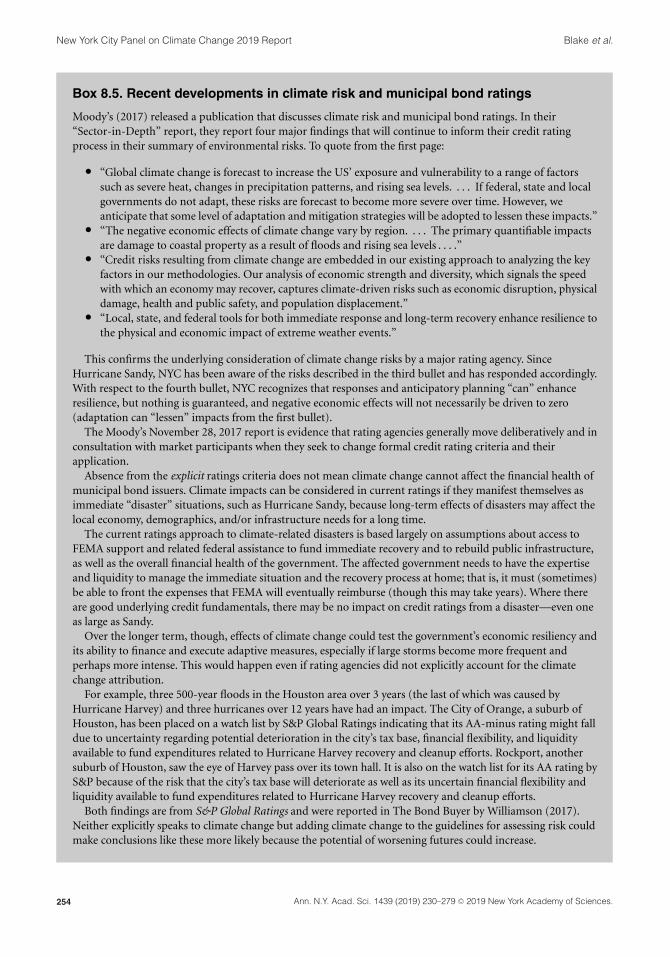
New York City Panel on Climate Change 2019 Report Blake et al.
Box 8.5. Recent developments in climate risk and municipal bond ratings
Moody’s (2017) released a publication that discusses climate risk and municipal bond ratings. In their“Sector-in-Depth” report, they report four major findings that will continue to inform their credit ratingprocess in their summary of environmental risks. To quote from the first page:
� “Global climate change is forecast to increase the US’ exposure and vulnerability to a range of factorssuch as severe heat, changes in precipitation patterns, and rising sea levels. . . . If federal, state and localgovernments do not adapt, these risks are forecast to become more severe over time. However, weanticipate that some level of adaptation and mitigation strategies will be adopted to lessen these impacts.”
� “The negative economic effects of climate change vary by region. . . . The primary quantifiable impactsare damage to coastal property as a result of floods and rising sea levels . . . .”
� “Credit risks resulting from climate change are embedded in our existing approach to analyzing the keyfactors in our methodologies. Our analysis of economic strength and diversity, which signals the speedwith which an economy may recover, captures climate-driven risks such as economic disruption, physicaldamage, health and public safety, and population displacement.”
� “Local, state, and federal tools for both immediate response and long-term recovery enhance resilience tothe physical and economic impact of extreme weather events.”
This confirms the underlying consideration of climate change risks by a major rating agency. SinceHurricane Sandy, NYC has been aware of the risks described in the third bullet and has responded accordingly.With respect to the fourth bullet, NYC recognizes that responses and anticipatory planning “can” enhanceresilience, but nothing is guaranteed, and negative economic effects will not necessarily be driven to zero(adaptation can “lessen” impacts from the first bullet).
The Moody’s November 28, 2017 report is evidence that rating agencies generally move deliberatively and inconsultation with market participants when they seek to change formal credit rating criteria and theirapplication.
Absence from the explicit ratings criteria does not mean climate change cannot affect the financial health ofmunicipal bond issuers. Climate impacts can be considered in current ratings if they manifest themselves asimmediate “disaster” situations, such as Hurricane Sandy, because long-term effects of disasters may affect thelocal economy, demographics, and/or infrastructure needs for a long time.
The current ratings approach to climate-related disasters is based largely on assumptions about access toFEMA support and related federal assistance to fund immediate recovery and to rebuild public infrastructure,as well as the overall financial health of the government. The affected government needs to have the expertiseand liquidity to manage the immediate situation and the recovery process at home; that is, it must (sometimes)be able to front the expenses that FEMA will eventually reimburse (though this may take years). Where thereare good underlying credit fundamentals, there may be no impact on credit ratings from a disaster—even oneas large as Sandy.
Over the longer term, though, effects of climate change could test the government’s economic resiliency andits ability to finance and execute adaptive measures, especially if large storms become more frequent andperhaps more intense. This would happen even if rating agencies did not explicitly account for the climatechange attribution.
For example, three 500-year floods in the Houston area over 3 years (the last of which was caused byHurricane Harvey) and three hurricanes over 12 years have had an impact. The City of Orange, a suburb ofHouston, has been placed on a watch list by S&P Global Ratings indicating that its AA-minus rating might falldue to uncertainty regarding potential deterioration in the city’s tax base, financial flexibility, and liquidityavailable to fund expenditures related to Hurricane Harvey recovery and cleanup efforts. Rockport, anothersuburb of Houston, saw the eye of Harvey pass over its town hall. It is also on the watch list for its AA rating byS&P because of the risk that the city’s tax base will deteriorate as well as its uncertain financial flexibility andliquidity available to fund expenditures related to Hurricane Harvey recovery and cleanup efforts.
Both findings are from S&P Global Ratings and were reported in The Bond Buyer by Williamson (2017).Neither explicitly speaks to climate change but adding climate change to the guidelines for assessing risk couldmake conclusions like these more likely because the potential of worsening futures could increase.
254 Ann. N.Y. Acad. Sci. 1439 (2019) 230–279 C© 2019 New York Academy of Sciences.
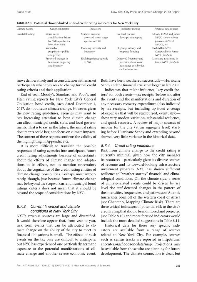
Blake et al. New York City Panel on Climate Change 2019 Report
Table 8.10. Potential climate-linked critical credit rating indicators for New York City
Climate hazard Generic indicator Indicators Indicator metrics Potential data sources
Coastal flooding Storm surgeamplification drivenby NYC-specific sealevel rise (SLR)
Sea level rise andprojected storm surgespecific to NYC
Sea level rise andflood-plain mapping
NOAA, FEMA and futureNPCC climate scienceproducts: NPCC4,NPCC5, etc.
Vulnerableproperties—publicand private
Flooding intensity andfrequency
Highway, subway, andproperty flooding
DoT, MTA, NYCComptroller & futureNPCC products
Projected changes inhurricane frequencyand intensity
Evolving science-specificto NYC
Observed frequency andintensity of east coasthurricanes possible foreach subway line
Literature as assessed infuture NPCC products
move deliberatively and in consultation with marketparticipants when they seek to change formal creditrating criteria and their application.
End of year, Moody’s, Standard and Poor’s, andFitch rating reports for New York City’s GeneralObligation bond credit, each dated December 1,2017, do not discuss climate change. However, giventhe new rating guidelines, agencies may want topay increasing attention to how climate changecan affect municipal credit, state, and local govern-ments. That is to say, in the future, the annual ratingdocuments could begin to focus on climate impacts.The content of these reports confirms the validity ofthe highlighting in Appendix 8.G.
It is more difficult to translate the possibleresponses of rating agencies into anticipated futurecredit rating adjustments because of uncertaintyabout the effects of climate change and adapta-tions to its effects, not to mention uncertaintyabout the cognizance of the credit rating entities ofclimate change possibilities. Perhaps most impor-tantly, though, just because future climate changemay be beyond the scope of current municipal bondratings criteria does not mean that it should bebeyond the scope of considerations by NYC.
8.7.3. Current financial and climateconditions in New York City
NYC’s revenue sources are large and diversified.It would therefore appear that, from year to year,risk from events that can be attributed to cli-mate change on the ability of the city to meet itsfinancial obligations is small. The effects of suchevents on the tax base are difficult to anticipate,but NYC has experienced one particularly germaneexposure to the potential manifestations of cli-mate change and another severe economic event.
Both have been weathered successfully—HurricaneSandy and the financial crisis that began in late 2008.
Indicators that might influence “key credit fac-tors” for both events—tax receipts (before and afterthe event) and the manifestations and duration ofany necessary recovery expenditure (also indicatedby tax receipts, but including up-front coverageof expenses that will be reimbursed, eventually)—show very modest variation, substantial resilience,and quick recovery. A review of major sources ofincome for the city (at an aggregate level) start-ing before Hurricane Sandy and extending beyondshowed very little variance in the historical data.
8.7.4. Credit rating indicatorsRisk from climate change to the credit rating iscurrently minimal, given how the city managesits resources—particularly given its diverse sourcesof revenue and its forward-looking infrastructureinvestment program. NYC has shown sufficientresilience to “weather stormy” financial and clima-tological conditions. On the climate side, a seriesof climate-related events could be driven by sealevel rise and detected changes in the pattern ofthe intensities, frequencies, and pathways of Atlantichurricanes born off of the western coast of Africa(see Chapter 5, Mapping Climate Risk). There arethree critical indicators of potential risk to the city’scredit rating that should be monitored and projected(see Table 8.10) and more focused indicators wouldinclude the more detailed suggestions in Table 8.11.
Historical data for these very specific indi-cators are available from a range of sourcesrelated to New York City. For example, sourcessuch as census tracks are reported in http://furmancenter.org/floodzonedata/map. Projections maybe available from those who are planning for futuredevelopment. The climate connection is clear, but
255Ann. N.Y. Acad. Sci. 1439 (2019) 230–279 C© 2019 New York Academy of Sciences.

New York City Panel on Climate Change 2019 Report Blake et al.
Table 8.11. Potential detailed coastal flooding indicatorsrelated to New York City credit rating
1. Estimated total housing units in floodplains
2. Estimated total renter-occupied housing units in floodplains
3. Estimated share in percent of all housing units that are in
floodplains
4. Estimated share in percent of floodplain housing units that
are in 2+ unit buildings
5. Estimated share in percent of floodplain housing units that
are located in buildings built before 1960
6. Estimated total subsidized rental housing units in floodplains
7. Estimated poverty rate in floodplains
they have not yet been quantified; and so projectionsinto the medium- and long-term risk, in terms oflikelihood, cannot be reported.
In terms of risk calculations that include bothlikelihood and consequence, the first two reflectongoing challenges—the first addresses likelihoodof a significant source of economic and social dam-age, while the second highlights consequence interms of economic value and therefore to somedegree the stability of the city’s tax base. The thirdalso incorporates likelihood, but suggests monitor-ing both observed data as reported by the NationalWeather Service and the scientific literature thatlinks detected deviations in hurricane experiencewith attribution to the increases in global mean tem-perature.
Increases in global mean temperature also driveconfirmed observations of rising sea levels aroundthe globe and increases in the frequency and inten-sity of extreme precipitation, but sea level rise isamplified in New York City (see Chapter 2, ClimateScience and Chapter 3, Sea Level Rise) and an imper-vious topography collects water in specific locations.Future iterations of the climate science chapters offuture NPCC reports will be critical in tracking andreporting all of these indicators.
8.8. Indicators of aggregate economichealth
Decision makers frequently ask for aggregate eco-nomic data about the potential costs of climatechange. Hsiang et al (2017) is one of the best avail-able examples of a rigorous analysis designed toaggregate those damages for the United States. Sev-eral observations can be drawn from their work:
1. Their estimates are based on selected availablelocal analyses. New York City is included for
coastal vulnerability for storms like HurricaneSandy as well as more ordinary coastal stormsand other extreme precipitation events.
2. Their estimates can now be tracked not onlyto temperature change, but also to transientdamages along collections of global green-house emissions trajectories that are targeted,along median scenarios, to specific tempera-ture targets like 1.5, 2.0, 2.5, and 3.0°C (Yohe,2017).
3. Those trajectories also reflect uncertaintyaround transient temperature increases basedon calibrations of scientific uncertainty. Theycan be downscaled to specific localities likeNYC, and they can also be expanded to reflectnoneconomic reasons for concern (like mor-tality driven by extreme heat).
4. Their economic estimates are dominated byrigorous but contentious estimates of the sta-tistical value of life—a contentious concept atbest.
Finally, Hsiang, et al (2017) confirm a conclu-sion that was perhaps first articulated forcefullyin the contribution of Working Group II (Chapter18 (IPCC, 2001a)) as well as both the SynthesisReport for Working Group II and the synthesisreport for the IPCC Third Assessment and (IPCC,2001b)—economic estimates are:
(1) Incomplete in their coverage of all economicsectors; and
(2) Missing the ameliorating effects of adaptation.
So they are, simultaneously, underestimates(because they miss damages) and overestimates(because they do not include adaptation). Thisis why most assessments, including the NationalClimate Assessment (NCA, 2014), and the fourthand fifth IPCC assessments (2007a, b and 2014a,b), shy away from reporting aggregate economicdamages.
By way of contrast, municipal credit ratings offergross measures of economic health and resilienceon the basis of the reliability of sources of local taxrevenue (the sources of revenue to pay back principleas well as annual interest obligations).
Now that credit ratings are explicitly recognizingeconomic risks from climate change from histori-cal data and projections, the credit rating agencies
256 Ann. N.Y. Acad. Sci. 1439 (2019) 230–279 C© 2019 New York Academy of Sciences.

Blake et al. New York City Panel on Climate Change 2019 Report
are taking up this challenge. They are now begin-ning to include considerations of projected adap-tations, diversification across revenue sources, andthe capacity to respond to disastrous climate-drivenevents without facing measurable fiscal stress.
Future credit ratings may well include consider-ation of the complicated risks that climate changeposes. These need to be included in economic mea-sures of vulnerabilities calibrated in useful metricsthat can be translated into fiscal stress on sources ofbond security. The results are aggregate expressionsof economic risk calibrated not by dollars directly,but by letter grades. AAA is better than AA andboth are much better than BB. The economic healthof NYC vis-a-vis climate-related risk is better thanHouston’s. It follows that simply following creditratings for specific locations (and for specific typesof projects with different time horizons) is a usefulindicator of the city’s financial health.
8.9. Implementation of the proposedNYCLIM
An effective, meaningful, and comprehensivecity-wide response to ongoing climate change willrequire an operational, systematic, centralizedcoordination of I&M networks, climate and socialscientists, stakeholders, federal, regional, andlocal data collection agencies and monitoringpartnerships, policy makers, citizen scientists, andempowered local community people. Such anorganized system of agencies, people, and resourcescreates a community of practice that enhances theclimate resilience process, its practice, and its deci-sions. Proper protocols for the process of selectingand systematically monitoring of key indicatorsand proper protocols for resiliency and for flexibleadaptation pathways may then be co-generated,implemented, and sustained. The proposedNYCLIM is envisioned to be such a system. Theall-encompassing goal would be to contribute tostate-of-the-art resiliency and adaptation strategiesfor New York City and its surrounding region.
8.10 Conclusions and recommendations
Concluding remarks are outlined below in severalcategories—key indicators, proposed I&M system,recommendations for policy, and recommendationsfor research.
8.10.a. Key indicatorsAfter studying the transportation and energy sec-tors and their interdependencies as depicted inFigure 8.3, the following indicators have been iden-tified as important in the context of climate changein regard to salience, accuracy, and accessibility.
Transportation
� Number, frequency, extent, and duration offacility and material damages to road and railsystems
� Extent and cost of service delays to road andrail users
Energy
� Magnitude of the number, frequency, geo-graphic extent, and duration of service outages
� Extent, cost, and inconvenience of electricpower service delays in terms of SAIDI andSAIFI—if they can be enhanced to reflectweather and climate-related impacts as well asto incorporate and adapt tools such as bene-fit and cost calculators for energy disruptions(e.g., U.S. DOE, Lawrence Berkeley NationalLaboratory, 2018).
Interdependencies
� Influence, in terms of likelihood and severity,of the combination of climate extremes anddependent and interdependent infrastructureconnections on infrastructure services
� Calibrated risk factors and infrastructurerecovery rates for dependent and interdepen-dent infrastructures
The above list is by no means comprehensive, butit addresses those that have been most commonlyidentified in the extensive literature upon whichTables 8.4, 8.5, and 8.8 are based and expanded inTables 7.1-3 in Chapter 7.
8.10.b. Proposed I&M System1. Climate and extreme weather events are
critical stressors. Their impacts upon infras-tructure have commonly been identified aspotential factors (see Chapter 7); however,finding performance indicators that are not
257Ann. N.Y. Acad. Sci. 1439 (2019) 230–279 C© 2019 New York Academy of Sciences.

New York City Panel on Climate Change 2019 Report Blake et al.
influenced by non-climate events (so-calledconfounding factors) can be difficult. Theirinfluences make detection and attributiondifficult and uneven. In short, attributionis now and will likely remain a significantchallenge. For forward-looking adaptation,though, attribution is essential in order toaddress fundamental causes of risk and torefine adaptation approaches.
2. A centralized, coordinated, I&M system forNYC, where specific roles, responsibilities, andinteraction or coordination are identified (asimplied in the proposed NYCLIM), is essen-tial for comprehensive, city-wide risk assess-ment and course-correction toward climatechange adaptation and resiliency goals and tar-gets. This recommendation for considerationis especially important for the design of short-to medium- to long-term selected investmentstargeted to adaptation.
The system should incorporate a consis-tent set of measures in order to capturechanges in climate conditions, goals, and tar-gets over time. City government, scientists,and other interested and responsible partiesare the drivers of this process.
3. An effective I&M system must be sufficientlyrobust and comprehensive to track key climatevariables and to associate ranges of possiblefuture states to ranges of possible adaptationstrategies. The system must accommodatevarious options so that it can identifyvulnerabilities and adaptation measuresrelated to observed conditions and/or theirprojected futures.
4. Spatial and temporal-scale resolutions needto be consistent and comparable across sec-tors if the I&M system is to detect effectivelytrends and differences across sectors and toallow for qualitative and/or quantitative com-parisons. That is to say, the people who acceptresponsibilities distributed across spatial, tem-poral, and actors defined in the proposedNYCLIM must be able to confer with eachother using a consistent vocabulary, and themeasures themselves should include those thatare consistent over time.
5. The construct of three broad time horizons(see the Appendix 8.E. for details)—long term(2080s, 2100, and beyond), medium term
(2050s), and short term (2020s)—and theboundaries between them have been instruc-tive in framing risk-related indicators andtheir uncertainties from one application ofindicators to another. The boundaries betweenthose three periods may need adjustment inresponse to how the future evolves.
6. Creating a set of preliminary, co-generateddecision-support indicators for the energy andtransportation sectors and selected depen-dencies and interdependencies among infras-tructure sectors has been identified as acritical element in support of the city’s adap-tive responses to promote resilience.
7. Key findings related to financial indicatorsinclude:� Credit ratings for specific locations (and
for specific types of projects with differ-ent time horizons) are useful indicators, aswell, because they are consistently craftedby independent experts working separately.
� Climate vulnerability of the city’s stable AAcredit rating is small (stable through thefinancial crisis and Hurricane Sandy).
8.10.c. Policy recommendations� New York City should take on the responsi-
bility to coordinate a climate indicator andmonitoring system across multiple gover-nance entities that provides periodic analyticalreports on indicator trends to aid in policy,planning, and financial decisions. The goalis to protect the region’s citizens and assetsunder changing climate conditions. In orderto accomplish this, the city should:
– Develop and implement the pro-posed New York City Climate ChangeResilience Indicators and MonitoringSystem (NYCLIM) that defines scope,explicitly provides information onrelevant spatial and temporal scales, andfacilitates integration across agencies,levels of governance, sectors, and spatialand temporal scales.
– Designate one of its agencies and an aca-demic partner to oversee its operations(community engagement, stakeholderinteractions, data collection, storage and
258 Ann. N.Y. Acad. Sci. 1439 (2019) 230–279 C© 2019 New York Academy of Sciences.

Blake et al. New York City Panel on Climate Change 2019 Report
management, analysis, personnel andfunding, etc.).
– Facilitate a co-generation process forthe development and dissemination ofthe NYCLIM that involves communityengagement and regional stakeholdersthrough time.
– Support evaluation and iterative researchon indicators and monitoring.
8.10.d. Recommendations for researchNPCC3 makes the following recommendationsfor continued research to improve the New YorkCity Climate Change Resilience Indicators andMonitoring System (NYCLIM) and address ongo-ing climate risks in the New York metropolitanregion:
� Analyze how and to what extent indicatorscan be linked to current and future resiliencedecision making under changing climate con-ditions, including the increasing frequency ofextreme events.
� Develop improved datasets for extreme eventsand system failures related to the transporta-tion and energy sectors (and other sectors aswell), and utilize multifactor analysis tech-niques to understand complex trends in vari-ables that affect service provision.
� Quantify economic and/or financial impacts ofclimate risks for use by credit rating agenciesand other third-party stakeholders.
Acknowledgments
The NPCC3 Indicators and Monitoring authorsthank all the New York City agencies and regionalorganizations that contributed to the Indicators andMonitoring chapter.
References
Allen, G. 2016. As Waters Rise, Miami Beach Builds HigherStreets and Political Willpower. In NPR. All Things Con-sidered, National Public Radio. May 10, 2016, 4:39PM ET.Accessed January 28, 2019. http://www.npr.org/2016/05/10/476071206/aswaters-rise-miami-beach-builds-higher-streets-and-political-willpower.
Associated Press. 2017. Five years after Sandy, recovery rocky inplaces. Chicago Tribune.
Bartos, M., M. Chester, N. Johnson, et al. 2016. Impacts of risingair temperatures on electric transmission ampacity and peak
electricity load in the United States. Environ. Res. Lett. 11:114008.
Burkett, V.R., A.G. Suarez, M. Bindi, et al. 2014. Point of depar-ture. In Climate Change 2014: Impacts, Adaptation, and Vul-nerability. Part A: Global and Sectoral Aspects. Contributionof Working Group II to the Fifth Assessment Report ofthe Intergovernmental Panel on Climate Change. 169--194.Cambridge, UK and New York, NY: Cambridge UniversityPress.
City of New York. 2013. Special initiative for rebuilding andresilience. PlaNYC: a stronger more resilient New York. pp. 1–438. Accessed June 11, 2013. http://www.nyc.gov/html/sirr/html/report/report.shtml.
Con Edison. Undated website. Smart meter installation.https://www.coned.com/en/our-energy-future/technology-innovation/smart-meters/when-will-i-get-my-smart-meter.
Con Edison. 2018. ConEdison AMI metrics report. New York,NY: ConEdison.
Dahlberg, T. 2006. Catenary, pantograph, and their interaction.Vehicle Systems Dynamics. Int J Veh Mech Mob. 44: 591–593.
Downing, T.E., R. Butterfield, S. Cohen, et al. 2001. Vulnerabilityindices: climate change impacts and adaptation. UNEP PolicySeries, UNEP, Nairobi.
Elfrink, T. 2016. Miami Beach’s Tidal Flooding Has Jumpedby 400 Percent in the Past Decade. In Miami NewTimes. April 6, 2016, 9:30AM. Accessed January 28, 2019.https://www.miaminewtimes.com/news/miami-beachs-tidal-flooding-has-jumped-by-400-percent-in-the-past-decade-8370816.
Eltman, F. 2017. NYC could see bad flooding every five years,study says. Bloomberg. Associated Press (AP).
Fawcett, A.A., G.C. Iyer, L.E. Clarke, et al. 2015. Can Parispledges avert severe climate change? Science 350: 1168–1169.
FTA 2011. Flooded Bus Barnes and Buckled Rails: PublicTransportation and Climate Change Adaptation. August2011. Accessed January 28, 2019. https://www.transit.dot.gov/sites/fta.dot.gov/files/FTA_0001_Flooded_Bus_Barns_and_Buckled_Rails.pdf.
Garner, A.J., M.E. Mann, K.A. Emanuel, et al. 2017. Impact of cli-mate change on New York City’s coastal flood hazard: increas-ing flood heights from the preindustrial to 2300 CE. Proc. Natl.Acad. Sci USA 114: 11861–11866.
Haimes, Y.Y., B.M. Horowitz, J.H. Lambert, et al. 2005. Inoper-ability input–output model for interdependent infrastructuresectors. I: theory and methodology. J. Infrastruct. Syst. 11:67–79.
Horton, R., C. Little, V. Gornitz, et al. 2015. New York City panelon climate change 2015 report chapter 2: sea level rise andcoastal storms. Ann. N.Y. Acad. Sci. 1336: 36–44.
Hsiang, S., R. Kopp, A. Jina, et al. 2017. Estimating economicdamage from climate change in the United States. Science356: 1362–1369.
Intergovernmental Panel on Climate Change (IPCC). 2001a.Report of working group II to the third assessment report. Cam-bridge, UK: Cambridge University Press.
Intergovernmental Panel on Climate Change (IPCC). 2001b. Syn-thesis report of the third assessment report. Cambridge, UK:Cambridge University Press.
Intergovernmental Panel on Climate Change (IPCC). 2007a.Report of working group II to the fourth assessment report. Cam-bridge, UK: Cambridge University Press.
259Ann. N.Y. Acad. Sci. 1439 (2019) 230–279 C© 2019 New York Academy of Sciences.
New York City Panel on Climate Change 2019 Report Blake et al.
Intergovernmental Panel on Climate Change (IPCC). 2007b. Syn-thesis report of the fourth assessment report. Cambridge, UK:Cambridge University Press.
Intergovernmental Panel on Climate Change (IPCC). 2014a.Report of working group II to the fifth assessment report. Cam-bridge, UK: Cambridge University Press.
Intergovernmental Panel on Climate Change (IPCC). 2014b. Syn-thesis report of the fifth assessment report. Cambridge, UK:Cambridge University Press.
Intergovernmental Panel on Climate Change (IPCC). 2014c.Chapter 19: emergent risks and key vulnerabilities. Cam-bridge, UK: Cambridge University Press.
Jacob, K., et al. 2011. Chapter 9: Transportation, in:Rosenzweig et al. (2011). Accessed January 28, 2019.www.nyserda.ny.gov/climaid.
Kaufman, S.M., C. Qing, N. Levenson, et al. 2012. Transportationduring and after Hurricane Sandy. New York, NY: New YorkUniversity, Rudin Center.
Metropolitan Transportation Authority (MTA). undated website. Performance data sets. Accessed June 16, 2017.http://web.mta.info/developers/performance.html.
Moody’s Investor Service. 2017. Evaluating the impact of climatechange on US state and local issuers.
MTA. 2008. MTA Blue Ribbon Commission on sustainabilitywater sustainability report. Accessed December 24, 2008.http://web.mta.info/sustainability/pdf/MTA%20Water%20Sustainability%20Report%20Final.pdf.
MTA 2017. MTA Climate Adaptation Task Force ResiliencyReport. Accessed January 28, 2019. http://web.mta.info/sustainability/pdf/ResiliencyReport.pdf.
National Academies, National Research Board, Transporta-tion Research Board. 2008. Potential impacts of climatechange on U.S. transportation. Washington, DC. AccessedDecember 16, 2018. http://onlinepubs.trb.org/onlinepubs/sr/sr290.pdf.
National Academies of Sciences, Engineering and Medicine.2016. Pathways to Urban Sustainability. Challenges and Oppor-tunities for the United States. Washington, D.C., The NationalAcademies Press.
National Research Council (NRC). 2010. Climate stabilizationtargets – emissions, concentrations, and impacts over decades tomillennia. National Academies Press.
NCA. 2014. National climate assessment. US Global ChangeResearch Program. Accessed December 16, 2018.nca2014.globalchange.gov/report/sectors/transportation;Box on Sandy, or download chapter in PDF from http://s3.amazonaws.com.
NYC Office of the Comptroller. 2015. A green bond program forNew York City New York. NY: NYC Comptroller. AccessedDecember 16, 2018. https://comptroller.nyc.gov/wp-content/uploads/documents/Green_Bond_Program_Update.pdf, p. 4Impact reporting.
NYS ISO. 2017a. 2017-Load & capacity data “gold book”. SeeTable “Forecast of Coincident Summer Peak Demand by Zone– MW” (NYC is zone J) can provide the basis for such anindicator.
NYS ISO. 2017b. Power trends report 2017. Accessed December16, 2018. http://www.nyiso.com/public/webdocs/media_room/publications_presentations/Power_Trends/Power_Trends/2017_Power_Trends.pdf.
New York City Panel on Climate Change (NPCC). 2010. Cli-mate Change Adaptation in New York City. New York
City Panel on Climate Change 2010 Report. Annals ofthe New York Academy of Sciences. 1196. New York, NY.Accessed February 2, 2019. https://nyaspubs.onlinelibrary.wiley.com/toc/17496632/1196/1
Rinaldi, S.M., J.P. Peerenboom & T.K. Kelly. 2001. Identifying,understanding, and analyzing critical infrastructure interde-pendencies. IEEE Contr. Syst. 21: 11–25.
Rosenzweig, C. & W. Solecki. 2018. Action pathwaysfor transforming cities. Nat. Clim. Change 8: 756–759.https://doi.org/10.1038/s41558-018-0267-x.
Rosenzweig, C. et al. 2010. Climate change adaptation in NewYork City: building a risk management response. The NewYork City Panel on Climate Change 2010 Report. Ann. N.Y.Acad. Sci. 1196: 1–354.
Rosenzweig, C. et al. 2015. Foreword to building the knowledgebase for climate resiliency: New York City Panel on ClimateChange 2015 Report. Ann. N.Y. Acad. Sci. 1336: 6.
Rosenzweig, C., W. Solecki, A. DeGaetano, et al. 2011. Respond-ing to climate change in New York State: the ClimAID inte-grated assessment for effective climate change adaptationin New York State. Final report. Ann. N.Y. Acad. Sci. 1244:2–149.
Rosenzweig, C., W.D. Solecki, P. Romero-Lankao, et al. 2018.Climate Change and Cities: Second Assessment Report of theUrban Climate Change Research Network. Cambridge Univer-sity Press.
Standard and Poors. What are rating criteria? Accessed Decem-ber 21, 2015. http://www.standardandpoors.com/ratings-direct.
T&D World Magazine. 2016. ConEd implementing new AMIprogram. T&D World Magazine. Accessed December 16,2018. http://www.tdworld.com/ami/coned-implementing-new-ami-program.
U.S. Climate Change Science Program. 2008. Impacts ofclimate change and variability on transportation systemsand infrastructure: Gulf Coast study, phase I. Synthesis andAssessment Product 4.7. Accessed December 16, 2018. https://www.globalchange.gov/browse/reports/sap-47-impacts-climate-change-and-variability-transportation-systems-and.
U.S. Department of Energy (U.S. DOE). 2009. Com-paring the impacts of the 2005 and 2008 hurri-canes on U.S. energy infrastructure. Accessed Decem-ber 16, 2018. http://www.oe.netl.doe.gov/docs/HurricaneComp0508r2.pdf.
U.S. Department of Homeland Security. National InfrastructureProtection Plan (NIPP). 2013. Accessed December 16,2018. https://www.dhs.gov/sites/default/files/publications/national-infrastructure-protection-plan-2013-508.pdf.
U.S. Department of Homeland Security. 2015. Sector-specificplans. https://www.dhs.gov/2015-sector-specific-plans.
U.S. Department of Transportation (DOT), FHWA, Officeof Planning, Environment, & Realty (HEP). 2015.Tools. Climate change adaptation. Sensitivity matrix.Accessed December 16, 2018. https://www.fhwa.dot.gov/environment/sustainability/resilience/tools/.
U.S. DOE. 2013a. Comparing the impacts of northeast hurri-canes on energy infrastructure. Accessed December 16, 2018.
260 Ann. N.Y. Acad. Sci. 1439 (2019) 230–279 C© 2019 New York Academy of Sciences.
Blake et al. New York City Panel on Climate Change 2019 Report
http://energy.gov/sites/prod/files/2013/04/f0/Northeast%20Storm%20Comparison_FINAL_041513c.pdf.
U.S. DOE. 2013b. U.S. energy sector vulnerabilities to climatechange and extreme weather. https://energy.gov/sites/prod/files/2013/07/f2/20130710-Energy-Sector-Vulnerabilities-Report.pdf.
U.S. DOE. 2014. The water–energy nexus: challenges and oppor-tunities. Washington, DC. Accessed December 16, 2018.https://www.energy.gov/sites/prod/files/2014/07/f17/Water%20Energy%20Nexus%20Full%20Report%20July%202014.pdf.
U.S. DOE, Lawrence Berkeley National Laboratory. 2018. Inter-ruption cost estimate (ICE) calculator. Accessed Decem-ber 16, 2018. https://eaei.lbl.gov/tool/interruption-cost-estimate-calculator.
U.S. DOE, Pacific Northwest National Lab (PNNL). 2016.Electricity distribution system baseline report. Richland,WA:PNNL. Accessed December 16, 2018. https://www.energy.gov/sites/prod/files/2017/01/f34/Electricity%20Distribution%20System%20Baseline%20Report.pdf.
The United States Environmental Protection Agency (EPA).2017. Climate change indicators in the United States. https://www.epa.gov/climate-indicators.
The United States Global Change Research Program (USGCRP).Accessed December 16, 2018. http://www.globalchange.gov/browse/indicators.
Wasserman, S. & K. Faust. 1994. Social Network Analysis: Methodsand Applications. Cambridge University Press.
Wdowinski, S., R. Bray, B.P. Kirtman, et al. 2016. Increasingflooding hazard in coastal communities due to rising sea level:Case study of Miami Beach, Florida. Ocean Coast Manag. 126:1–8. Accessed January 28, 2019. http://www.sciencedirect.com/science/article/pii/S0964569116300278.
Williamson, R. 2017. Harvey’s impact on credit becoming moreapparent – 500-year floods every 5 years could start by 2030.The Bond Buyer, October 2.
Yohe, G.W. 2017. Characterizing transient temperature trajecto-ries for assessing the value of achieving alternative tempera-ture targets. Clim. Change 145: 469–479.
Zimmerman, R. 2004. Decision-making and the vulnerability ofinterdependent critical infrastructure. In 2004 IEEE Interna-tional Conference on Systems, Man and Cybernetics, IEEE, Vol.5, pp. 4059–4063.
Zimmerman, R. 2014. Planning restoration of vital infrastruc-ture services following Hurricane Sandy: lessons learnedfor energy and transportation. J Extreme Events 1:1450004.
Zimmerman, R. & C.E. Restrepo. 2006. The next step: quan-tifying infrastructure interdependencies to improve secu-rity. Int. J. Crit. Infrastruct. 2: 215–230. Summarized fromTable 3.
Zimmerman, R. & C.E. Restrepo. 2009. Analyzing cascadingeffects within infrastructure sectors for consequence reduc-tion. In IEEE Conference on Technologies for Homeland Secu-rity, 2009. HST’09. IEEE, pp. 165–170.
Appendix 8.A. Further details onstakeholder engagement andco-generation process for Chapter 8,Indicators and Monitoring, and proposedNYCLIM
The I&M Work Group held a roundtable withthe CCATF on Wednesday, March 9, 2016. Twenty-seven CCATF and NPCC members participated inthe workshop, as well as individuals from city agen-cies, including the New York City Office of Recoveryand Resiliency, the Department of City Planning,and the Department of Environmental Protection.The workshop featured two of the main architects ofthe Indicators and Monitoring System section of theU.S. National Climate Assessment—Dr. AnthonyJanetos and Dr. Melissa Kenney. Dr. Janetos led theworkshop and made a presentation on “Develop-ing a pilot indicator system for U.S. climate changes,impacts, vulnerabilities, and responses.” From thisroundtable, a list of resiliency indicators alreadybeing tracked by stakeholder attendees was devel-oped. A key action item from the roundtable was tobegin a “straw-man” of the pilot for a coordinatedway of tracking these and other relevant indicatorsfor the five CCATF-NPCC3 sectors.
On July 27, 2016, a joint CCATF-NPCC meetingwas held. Participants included about 40 CCATFstakeholders and 13 NPCC3 members. The break-out sessions at the workshop were devoted to gettinginput from the CCATF members across the work-groups on their I&M needs. Stakeholders reflectedon potential climate and impact indicators withineach of their sectors, and notes were collected fromthose discussions. The main message from this jointmeeting was to create a system that will allow indica-tors of climate change to be able to inform decisionmaking and facilitate NPCC3 research into decision-making contexts.
Throughout the process, a plethora of iterativeconversations and meetings that fostered the I&Mco-generation process were held between the I&MWork Group and stakeholders. Moreover, a memberof the author team who is also a member of theNPCC3 leadership regularly attended and partici-pated in CCATF meetings. The main stakeholdersinvolved in the co-generation process includedthe following: The Metropolitan TransportationAuthority, The NYC Department of Transportation,
261Ann. N.Y. Acad. Sci. 1439 (2019) 230–279 C© 2019 New York Academy of Sciences.

New York City Panel on Climate Change 2019 Report Blake et al.
The NYC Department of Environmental Protection,Port Authority of New York and New Jersey, EasternGeneration, The NYC Emergency ManagementOffice, and The NYC Comptroller’s Office.
Appendix 8.B. Short introduction todetection and attribution
In communicating degrees of certainty in the find-ings, the IPCC (2014a) reported a greater confidencein the projection of climate change-related phenom-ena than in the detection and attribution of observedimpacts (see Fig. 8.B.1). Working from this conclu-sion, it is important to investigate two fundamentalquestions:
How can confidence in projected vulnerabilities andimpacts be greater than confidence in attributing whathas heretofore been observed in ways that are consistentwith expectations derived from statistical foundations?
Are there characteristics of recent historical data seriesthat portend achieving high confidence in attribution toclimate change?
That is, one might expect that confidence inattribution-based projection should decrease out-side the sample domain due to the inherent vari-ability of future outcomes. Why is this not reflectedin the IPCC results? It turns out that the long-term nature of adaptation and mitigation strategyplanning and the requisite understanding of theunderlying physical and social processes by whichconfidence in projections can legitimately be evalu-ated can illuminate the foundations of strategies foriterative risk management and that they also explainwhat might otherwise be viewed both as a contra-diction of rigor and an obstacle for rigorous policyevaluation.
To demonstrate how confidence in projectioncan be higher than confidence in attribution ofa detected phenomenon, it is necessary to inves-tigate the effects of confounding factors imposed,for example, by site-specific socioeconomic devel-opment pathways in the context of climate change.These are effects that must be considered when
Figure 8.B.1. Higher confidence in projected outcomes versusobserved outcomes. Source: Figures 1–6 with reference to Tables1 and 2 in Burkett et al. (2014).
attributing observed climate change to associatedincreases in risk and using that attribution to createprojections into the future. They explain why thescience supports attribution of the recent droughtin the Southwest to anthropogenic warming, whileit does not yet support a similarly conclusion for therecent California drought where diverse topographyand the proximity of an ocean confound the statis-tics of what would seem to be a straight forwardattribution. Based on a growing number of obser-vations indicating the unequivocal nature of theobserved climate warming trend, though, we shouldexpect that the impact of climate change, and conse-quentially the “climate signal,” would increase withtime, while the impact of confounding variables likegeographical characteristics could be expected toremain static or at least trend less significantly. Asa result, the relative strength of the climate changesignal can be enhanced over time and explain theunderlying foundation of the Figure 8.B.1 results.
262 Ann. N.Y. Acad. Sci. 1439 (2019) 230–279 C© 2019 New York Academy of Sciences.

Blake et al. New York City Panel on Climate Change 2019 Report
Appendix 8.C. Catalogs of existing indicators of climate change
Table 8.C.1. A sample of indicators from U.S. Federal agencies and administrations
Environmental Protection Agency (EPA) climate indicators
Source: https://www.epa.gov/climate-indicators.
Indicator
Emissions
GHG emissions by type (gT;CO2e) National and Global since 199 (X)
GHG emissions and sinks (gT;CO2e) by sector National and Global since 1990 (X)
by sector
GHG emissions per capita (gT;CO2e/pop) National since 1990 (X)
GHG emissions per dollar (gT;CO2e/$) National since 1990 (X)
Weather and climate
Average temperature (oC)a
48 states and Global since 1990 (X)
Heat wave index (index #)a
National since 1890 (X)
Area of very hot summers (km2)a
48 states since 1910 (X)
Area of very cold winters (km2)a
48 states since 1948 (X)
Change in very hot summersa
48 states 1948–2015 (X)
Change in very cold wintersa
48 states 1950–2015 (X)
Precipitationa
48 states since 1901 (X)
Change in precipitationa
48 states and Global since 1901 (X)
Extreme 1-day precipitation (# days)a
48 states since 1901 (X)
Unusually high precipitationa
48 states since 1895 (X)
Hurricanes and cyclone (power indices) North Atlantic since 1860 (X)
Change in riverine flooding: National 1965–2015 (X)
Change in magnitudea
National 1965–2015 (X)
Change in frequencya
National 1965–2015 (X)
Average drought conditions (PDSI) 48 states since 1890 (X)
Land under drought with five severity levels National and Southwest since 2000 (X;Y) X
Health
Heat-related deaths (# days)a
National since 1978 (X)
Summer deaths - heat and cardiovascular (#) National & Chicago since 1999 abd 1995 (X)
Heating and cooling degree days (#)a
National since 1890 (X)
Change in heating (# degree days)a
National since 1895 (X)
1895–1954
Change in cooling (# degree days)a
National since 1955 (X)
Lyme disease (# cases per year)a
National since 1990 (X)
Change in Lyme incidence (# cases)a
Northeast to Minnesota 1991–2015 (X;Y)
Minnesota
Change in Lyme incidence (# cases)a
Selected sites 1996 & 2015 (X;Y)
West Nile virus dispersion (# cases)a
National since 2000 (X)
Length of growing season (# days) 48 states since 1890 (X)
Change in season length (# days) 48 states 1895–2015 (X)
Change in first frost (# days) 48 states 1895–2015 (X)
Change in last frost (# days) 48 states 1895–2015 (X)
Continued
263Ann. N.Y. Acad. Sci. 1439 (2019) 230–279 C© 2019 New York Academy of Sciences.

New York City Panel on Climate Change 2019 Report Blake et al.
Table 8.C.1. Continued
Oceans
Land lost (km2) East coast since 1996 (X;Y)
Change in frequency of coastal floodinga
National 2010–2015 (X:Y)
Arctic sea ice (km2) Arctic Ocean since 1975 (X;Y)
Lake ice (km2) Selected locations since 1840 (X;Y)
Ice thawing date (# days) 48 states since 1905 (X;Y)
National Oceanographic and Atmospheric Administration (NOAA) climate indicators
Source: https://www.ncdc.noaa.gov.
Indicator
National temperature index National (X;Y;Z)
Climate rankings Global, national, regional (X;Y;Z)
Temperature (degrees C)a
(X;Y)
Precipitation (versus average)a
(X;Y)
Degree days (degree days) (X;Y)
Palmer drought index (X;Y)
Extremes: Global down to U.S. cities (X;Y;Z)
Climate extremes index
Very cold/hot (mean max and min)
(degrees C)a
Very wet/dry (mean max and min)
(versus average)a
Societal impacts: Global down to U.S. cities (X;Y;Z)
Crop moisture (index #)
Energy demand (index #)a
Air stagnation (index #)
Wind (mean monthly m/s)a
Wildfires (# and total acres)
Heat stress (index #)a
$1b climate disasters (#)a
1980–2017 (X;Y;Z)
Hurricanes (#/year)a
Tornadoes (#/year)
Other:
Sea level rise (mm/year)a
Local, national, global (X;Y;Z)
Arctic sea ice (km2 in April) (X;Y;Z)
Snow cover (km2 in April) Local, national, global (X;Y;Z)
Sea surface temperature Global, regional (X;Y;Z)
(degrees C)
ENSO, NAO, PDO, PNAa
(indices) Global, national, regional (X;Y;Z)
United States Global Change Research Program (USGCRP) climate indicators
Source: https://globalchange.gov/explore/indicators.
Indicator
Frost free season (difference from average # days) National average for 30 years (X)
Annual GHG index Global since 1980 (X)
Arctic sea ice (km2)a
Arctic Ocean (September since 1979 (X;Y) since 1979
Atmospheric CO2 (ppm CO2e) Global since 1980 (X)
Average surface temperature (degrees C) Global since 1980 (X)
Start of spring (difference from average (# days) 48 states since 1900 (X)
Annual terrestrial carbon storage (Gt C) 48 states since 2004 (X)
aThe denotation of indicators that are relevant to urban resilience at a local scale; these provide at least a larger scale context withwhich local indicators must be consistent.Note: Parenthetical notation reflects the character of the content of the files according to: “Historical Data” by X, “Graphical Plots”by Y, and Geographical Maps” by Z).
264 Ann. N.Y. Acad. Sci. 1439 (2019) 230–279 C© 2019 New York Academy of Sciences.

Blake et al. New York City Panel on Climate Change 2019 Report
Table 8.C.2. Other climate indicators related to infrastructure. National Academies (2016)
Indicator Metric and unitsGeographic Scopea /NYCvalues (bold, underlined)
Historical/time period(based on time indicated
in table or refs.)
Environmentala (National Academies, 2016: pp. 154–156)Air quality NAAQS PM2.5 ppm 10.8 2011
Air Quality Index (U.S. EPA)Total days#days exceeding goodmoderatemaximumMedian days
36613021415055
2012
Greenhouse gasemissions (CO2)
SMA 2010
Residentiala
commerciala
industriala
CO2 per capitaper GDPper GDP
1.80.01NA
Water quality Number of impaired waterways State only1543
2012
HydrologyPrecipitationa (average
annual)Inches/year 46.23 2016
Landslide vulnerability USGS index (low, medium, high) L 2014Tree coveragea % land coverage by canopy 21 2015Parks Acreage/1000 resid. 4.6 2014Ecological footprint Global hectares/capita 6.1Natural hazards
vulnerability# Events 1/1/05–6/1/15 656 1/1/05-6/1/15
Economica (National Academies, 2016: pp. 156–158)Employment% employees by U.S.
Census sector% of total employment Numerous 0.1–25.2% 2014
Financial strength Bond ratings AA 2014, 2015Median household
incomeDollars $53,107 2009-2013
Unemployment rate % Census based (population > 16years old)
7.2 2014
Energy (National Academies, 2016: p. 158)Usage rates: residentiala
commerciala
industriala
MMBtu/capitaper GDPper GDP
49.40.6NA
2005, 2010
Cost (residential)a Ave. cents per kWh 23.21 2005, 2010Disruptiona SAIDI 19.0 2011, 2013 (depending
on city)
Continued
265Ann. N.Y. Acad. Sci. 1439 (2019) 230–279 C© 2019 New York Academy of Sciences.

New York City Panel on Climate Change 2019 Report Blake et al.
Table 8.C.2. Continued
Indicator Metric and units
Geographic Scope/NYCvalues (bold,underlined)
Historical/timeperiod (based ontime indicated in
table or refs.)
Transportationa (National Academies, 2016: p. 158)Transportation mode % public transportation 58.7 Circa 2010Walkscorea Computed—out of 100
total88 NA
Usage:Road travel (United
States)a
Road travel (cities)a
Annual VMT, DVMT/cap U.S. 290,116Cities 16.3
2012
Licenses Licenses (driving age)/1000drivers
705 2013
Travel time Mean travel time to work(total in minutes)
44.6 2014
Road congestion TTI (automobiles)Annual delay(h/commuter)Fuel excess (gals.)Cost/commuter
7435
2015
Public transportationusea
Average weekday ridership 11,664 2014
Watera (National Academies, 2016: p. 158)Total water usage Gallons/cap/day CountyIndividual use Average gallons per
capita/dayCities75
2010
Sociala (National Academies, 2016: pp. 158–162; 164)Population Total individual population 8,491,079 2010Demographics Quantitative (not related to
CO2 without conversion)Multiple 2010
Housing Quantitative (not related toCO2 without conversion)
Multiple 2010
Education Quantitative (not related toCO2 without conversion)
Multiple 2010
Public safety Quantitative (not related toCO2 without conversion)
Multiple NA
Health Quantitative (not related toCO2 without conversion)
Multiple 2014
aData provided for Vancouver, Los Angeles, New York, Philadelphia, Pittsburgh, Chattanooga, Grand Rapids, Cedar Rapids, Flint,and the United States; however, the indicators are applicable to any cities and data sources cover a wide variety of other cities.NA, not available.Source: National Academies of Sciences, Engineering, and Medicine. 2016. Pathways to urban sustainability: challenges andopportunities for the United States. Washington, DC: The National Academies Press. https://www.nap.edu/catalog/23551/pathways-to-urban-sustainability-challenges-and-opportunities-for-the-united.Summary from Appendix B: Details for urban sustainability indicators (nine cities)Note: Starred indicators in bold are those extracted or summarized from NASEM (2016) most directly related to climate change;bolded and underlined values signify those specifically identified for NYC. Plots are not consistently used, however; spider diagramsare used for some of the indicators
266 Ann. N.Y. Acad. Sci. 1439 (2019) 230–279 C© 2019 New York Academy of Sciences.

Blake et al. New York City Panel on Climate Change 2019 Report
Table 8.C.2., ContinuedEconomic Intelligence Unit (EIU)
Indicator Metric and units Scope NYC values(bold, underlined)
Historical/time period
CO2 Global—city specificCO2 Intensity Total emissions (weight
a)/GDP 145
c2002
CO2 Emissions Total emissions per capita 8.6c
2002CO2 Reduction strategy quantitative amount of reduction achieved;
Qualitative: plan assessment;–
ENERGY [p. 91] Global—city specificEnergy consumption Gigajoules (GJ)/capita 64.7 2009
Energy intensity GJ or megaJ/GDPb
0.5 2009Renewable energy consumption Quantitative % of energy from renewable
sources (e.g., based on teraJ);Qualitative assessment
Clean and efficient energy policies Qualitative assessment of commitmentBuildings
aGlobal—city specific
Energy consumption of residential buildings #LEED certified buildings/100,000 persons 1.1 2010Energy-efficient building standards QualitativeEnergy-efficient building initiatives QualitativeTransport
a[p. 91]
cGlobal—city specific
Use of noncar transport % workers using noncar modes 37.2 2009Size of noncar transport network Availability of public transport including length of
system miles/miles2
1.8 2009
Ave. commute time Ave. commute time in minutes from residence towork (minutes)
34.6 2009
Annual vehicle revenue miles miles/person 68.5 2009Maximum public transport vehicles per square
mileVehicles/miles2 44.9 2009
Congestion reduction policies QualitativeWaste and land use
aGlobal—city specific
Municipal waste production Total annual municipal waste per capita(collection)
–
Waste recycling % recycled 30.4 2006Waste reduction policies Qualitative –Green land use policies Green space as % of total area 19.7 2008Water
aGlobal—city specific
Water consumption Ave. daily water consumption (gallons) per capita 69.3 2005System leakages % water leakage 14.2 2009Wastewater system treatment Stormwater management planWater efficient and treatment policies Qualitative
AIR QUALITYd
[p. 91] Global—city specificNitrogen dioxide Emissions (in lbs)/year/person 29 2005Sulfur dioxide Emissions (in lbs)/year/person 10 2005Ozone Emissions (in lbs)/year/person –Particulate matter Emissions (in lbs)/year/person 6 2005Clean air policies QualitativeEnvironmental governance
aGlobal—city specific
Green action plan QualitativeGreen management QualitativePublic participation in green policy QualitativeSocial
a[p. 88]
Wealth GDP/capita (in $s) 56,900Employment Goods employment % 9
Service employment % 91Population density [p. 91] Persons/sq miles 27,666.8 2009
aWeight measures vary for different continents.bBase years for GDP vary, for example, for Europe, it tends to be 2000.cData are for the MSA or Metro.dData are for county.Source: Extracted from Economist Intelligence Unit (EUI). 2012. The Green City Index. A summary of the Green City Index
research series. Munich, Germany: Siemens.Note: The Green City Index covers the United States and Canada (27 cities), Europe (30 cities), Asia (22 cities), Latin America
(17 cities), Africa (15 cities), and Australia and New Zealand (7 cities). The approximate date of the indices is 2012 though the datacan range from 2000 to 2012.
267Ann. N.Y. Acad. Sci. 1439 (2019) 230–279 C© 2019 New York Academy of Sciences.

New York City Panel on Climate Change 2019 Report Blake et al.
Table 8.C.2., ContinuedDependencies and interdependencies (see following tables for examples of indicators)
1. Recovery ratesa. Component-specific intraenergy relationships. U.S. Department of Energy (DOE). 2009.
Comparing the impacts of the 2005 and 2008 hurricanes on U.S. energy infrastructure.http://www.oe.netl.doe.gov/docs/HurricaneComp0508r2.pdf.
b. Electric power dependency-based recovery rates. Zimmerman, R. & C.E. Restrepo., 2006. The nextstep: quantifying infrastructure interdependencies to improve security. Int. J. Crit. Infrastruct. 2:215–230. Transportation, water, and industrial recovery rates based on dependence on electric powerand relative to when power was restored after the 2003 blackout.
2. Qualitative and quantitative interdependencies/dependencies among infrastructure sectorsa. Production/consumption-based interconnections (between water and energy)
U.S. DOE. 2014. The water–energy nexus: challenges and opportunities. Washington, DC: U.S. DOE.
b. Input–output (expressed as material flows and value in dollars)Example: Haimes et al., 2005. Inoperability input–output model for interdependent infrastructuresectors. I: theory and methodology. J. Infrastruct. Syst. 11: 67–79.
c. Network-based quantifications
Apostolakis, G.E. & D.M. Lemon., 2005. A screening methodology for the identification and ranking ofinfrastructure vulnerabilities due to terrorism. Risk Anal. 25: 361–376.
d. Interrelationships identified
Zimmerman, R. & C.E. Restrepo., 2009. Analyzing cascading effects within infrastructure sectors forconsequence reduction. In Proceedings of the HST 2009 IEEE Conference on Technologies for HomelandSecurity, Waltham, MA, pp. 165–170. http://ieeexplore.ieee.org/stamp/stamp.jsp?arnumber = 05168004Provides a table of interdependencies (qualitative) (see below); used in the U.S. DHS (2015) EnergySector Specific Plan.
3. Effects based on physical proximitya. Rinaldi, S., J. Peerenboom, T. Kelly. 2001. Identifying, understanding, and analyzing critical infras-
tructure interdependencies. IEEE Contr. Syst. Magazine 21: 11–25.b. Zimmerman, R., 2004. Decision-making and the vulnerability of critical infrastructure. In Proceed-
ings of IEEE International Conference on Systems, Man and Cybernetics, SMC 2004. W. Thissen, P.Wieringa, M. Pantic & M. Ludema, Eds.: 4059—4063, Volume 5. The Hague, The Netherlands: DelftUniversity of Technology. Case-based study of transportation, energy and water distribution systemdependencies.
268 Ann. N.Y. Acad. Sci. 1439 (2019) 230–279 C© 2019 New York Academy of Sciences.

Blake et al. New York City Panel on Climate Change 2019 Report
Table 8.C.2., ContinuedRecovery rates, interconnections, and physical effects
Indicator Metric Geographic scope Historical/timeperiod
Types ofinfrastructure
1. Recovery ratesa. U.S. Department of Energy (2009) Time in days for restoration of key energy
infrastructure after the 2005 and 2008Hurricanes
National Energy and water
b. Zimmerman and Restrepo (2006) Recovery time of one infrastructurerelative to another as: Ti/TeTi = sector recovery timeTe = energy recovery time
National (selectedplaces)
2003 Electricpower outage
Electric power;transportation(transit, road, air)andmanufacturing
2. Quantitative and qualitativeinterconnections
a. Component-specific linksU.S. Department of Energy (2014) Water for energy (by use category)
Numerous quantitative measures (tobe itemized)
EnergyWater
U.S. Department of Energy (2014) Energy for water (by use category)Numerous quantitative measures (tobe itemized)
EnergyWater
b. Input–outputHaimes et al. (2005) I/O relationships for $ exchanges among
sectorsIndustry level,United States
Numerous (basedon I/O)
c. Network-basedApostalakis and Lemon Network connection measures Industry level Energy and water
subsectorsd. Identification of interconnectionsZimmerman and Restrepo (2009) Qualitative3. Quantitative effects based on physical
proximitya. Rinaldi et al. (2001) Qualitative –b. Zimmerman (2004) Count of times one distribution disables
another and directionNational—casebased (80 cases)
Sectors generating and receiving service from another sector
Sector receiving the serviceSector generating the
service to another(receiving) sector
Energy: oil and gas Energy: electricity Transportation Water Communications
Energy: oil and gas Fuel to operate powerplant motors andgenerators
Fuel to operatetransport vehicles
Fuel to operate pumpsand treatment
Fuel to maintaintemperatures forequipment; fuel forbackup power
Energy: electricity Electricity forextraction andtransport (pumpsand generators)
Power for overheadtransit lines
Electric power tooperate pumps andtreatment
Energy to run celltowers and othertransmissionequipment
Transportation Delivery of suppliesand workers
Delivery of suppliesand workers
Delivery of suppliesand workers
Delivery of suppliesand workers
Water Production water Cooling andproduction water
Water for vehicularoperation; cleaning
Water for equipmentand cleaning
Communications Breakage and leakdetection andremote control ofoperations
Detection andmaintenance ofoperations andelectrictransmission
Identification andlocation of disabledvehicles, rails, androads; the provisionof user serviceinformation
Detection and controlof water supply andquality
Source: Zimmerman, R. & C.E. Restrepo., 2009. Analyzing cascading effects within infrastructure sectors for consequence reduc-tion. In Proceedings of the HST 2009 IEEE Conference on Technologies for Homeland Security, Waltham, MA, pp. 165–170.http://ieeexplore.ieee.org/stamp/stamp.jsp?arnumber = 05168004. This table was used in the U.S. DHS (2015) Energy Sector-SpecificPlan.
269Ann. N.Y. Acad. Sci. 1439 (2019) 230–279 C© 2019 New York Academy of Sciences.

New York City Panel on Climate Change 2019 Report Blake et al.
Appendix 8.D. Matrix to organizeinformation that defines an indicator
Figure 8.D.1 displays a matrix structure throughwhich this information can be displayed coherentlyand by which existing gaps in coverage can be dis-covered. This sample matrix shows how complexthe task is to pursue the development of valid andpurposeful indicators if executed in a rigorous way.
Figure 8.D.1. The matrix template for organizing information.
Figure 8.D.1 Legend: This 3-D generic matrix forindicators may apply, for instance, to the electricpower grid. Indicators for A: Climate Extreme, forexample for Weather Extremes; B: Impact; C: Vul-nerability D: Resilience. In each of these four indica-tor planes, there are (for energy) three hazards con-sidered (storms, heat waves, and cold spells), andfor the three time horizons (short, medium, andlong term). Each individual indicator (boxes) hasfour Attributes: P = Purpose (what is attemptedto be achieved when using this indicator); M =
Measurement (what variable or quantity is mea-sured); D = Definition (provides exact metrics andapplicable location where necessary); and S = DataSource (agency, differentiates between verified orexpected).
Figure 8.D.1 illustrates the complexities that ide-ally need consideration when devising indicators,with an example for just one of the infrastructure
systems (in this case, the electric energy grid).
There are intended to be four designated indica-tors A through D for each infrastructure type (cli-mate, impacts, vulnerability, and resilience; theywere earlier listed in Section XYZ); there are threetime horizons (short, medium, long); 3 hazard types(storms/SLR, heat, cold spells); and for each indi-cator, four attributes need to be defined (purpose,definition, metrics, source). If each indicator ele-ment were to be fully realized, this implies, that acombination of at least 4 × 3 × 3 × 4 = 144 indi-cator elements would have to be provided, for a
270 Ann. N.Y. Acad. Sci. 1439 (2019) 230–279 C© 2019 New York Academy of Sciences.
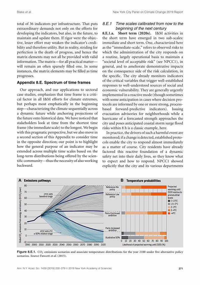
Blake et al. New York City Panel on Climate Change 2019 Report
total of 36 indicators per infrastructure. That putsextraordinary demands not only on the efforts fordeveloping the indicators, but also, in the future, tomaintain and update them. If rigor were the objec-tive, lesser effort may weaken the indicator’s credi-bility and therefore utility. But in reality, striding forperfection is the death of progress, and hence thematrix elements may not all be provided with validinformation. The matrix—for all practical matter—will remain an often sparsely filled one. In someinstances, the matrix elements may be filled as timeprogresses.
Appendix 8.E. Spectrum of time frames
Our approach, and our applications to sectoralcase studies, emphasizes that time frame is a criti-cal factor in all I&M efforts for climate extremes,but perhaps most emphatically in the beginningstep—characterizing the climate sequentially acrossa dynamic future while anchoring projections ofthe future onto historical data. We have noticed thatstakeholders look at time from the shortest timeframe (the immediate scale) to the longest. We beginwith this pragmatic perspective, but we also move ina second section of this Appendix to consider timein the opposite direction; our point is to highlighthow the general purpose of an indicator may beextended across multiple time scales based on thelong-term distributions being offered by the scien-tific community—thus the necessity of also workingbackward.
8.E.1 Time scales calibrated from now to thebeginning of the next century
8.E.1.a. Short term (2020s). I&M activities inthe short term have emerged in two sub-scales:immediate and short term. One, characterized hereas the “immediate-scale,” refers to observed risks towhich the administration of the city responds ona routine, largely operational basis to maintain a“societal level of acceptable risk” (see NPCC1), ingeneral, and to ameliorate demonstrative impactson the consequence side of the risk calculation, inthe specific. The city already monitors indicatorsof the critical variables that trigger well-establishedresponses to well-understood sources of social andeconomic vulnerability. They are generally urgentlyimplemented in a reactive mode (though sometimeswith some anticipation in cases where decision pro-tocols are informed by one or more strong, process-based forward-predictive indicators). Issuingevacuation advisories for neighborhoods while ahurricane of a forecasted strength approaches thecity and poses anticipated coastal storm surge floodrisks within 8 h is a classic example, here.
In practice, the drivers of such a harmful event aremonitored; if a change is detected, established proto-cols enable the city to respond almost immediatelyas a matter of course. City residents have alreadyfactored this reactive foundation of a dynamicsafety net into their daily lives, so they know whatto expect and how to respond. NPCC1 showedexplicitly that the city and its various departments
Figure 8.E.1. CO2 emissions scenarios and associate temperature distributions for the year 2100 under five alternative policyscenarios. Source: Fawcett et al. (2015).
271Ann. N.Y. Acad. Sci. 1439 (2019) 230–279 C© 2019 New York Academy of Sciences.

New York City Panel on Climate Change 2019 Report Blake et al.
Box 8.E.1. Annual likelihoods of experiencing 95th percentile or anomaloussummer heat (relative to the 1971 through 2000 historical record) during thesummer months in New York City
Working from the median “no-policy” baseline trajectory in Fawcett et al (2015, Fig. 8.E.1.) brings globalemissions to nearly 95 GtCO2 per year by the end of the century. It is defined by two boundary conditions. For2010, annual global emissions begin around 30 GtCO2 and grow initially at approximately 6% per year.Emissions reach 95 GtCO2 by 2100 because the rate of growth depreciates by 0.5% per year.
Corresponding transient temperature trajectories can be calculated from a linear relationship betweencontemporaneous cumulative emissions and transient temperature reported in NRC (2010, pages 102–103and Fig. 4.9): 1.75 °C per 1000 GtC is the median estimate. Higher and lower trajectories, here, are driven byuncertainty around the behavior of sinks in higher temperatures and around the sensitivity of the climate toexternal forcing: the 95th percentile temperature for any emissions total is 70% above the temperatureassociated with median, and the 5th percentile temperature is 40% below the median.
Constrained emissions pathways through 2100 can be anchored, for example, by two trajectories that limitthe median estimated increases in transient temperature to 1.5 °C and 2.0 °C above preindustrial levels (2.7°Fand 3.6°F; see Yohe, 2017). They are “ideal” and comparable in the sense that each of them reduces emissionsover time so as to maximize the discounted logarithmic-derived utility generated by emissions through 2100.That is to say, they solve two parallel Hotelling-style exhaustible resource problems where cumulativeemissions constraints derived from NRC (2010) serve as operating “supply” constraints on total emissions forthe two temperature targets: 1715 and 2575 GtCO2, respectively. The Hotelling results, with logarithmic utility,mean that emissions face downward exponential pressure relative to the initial 6% annual growth at a rateequal to the associated utility discount factor for each target.
Anticipated changes in the likelihood of experiencing the anomaly or 95th percentile summer heat everyyear are derived from NRC (2010, page 102). For reference, #ONENYC reports an average of two prolongedheat waves per year during the baseline observation period (1971–2000); NPCC portrays a plus or minus 2range in that estimate around that mean for the same historical period (see Chapter 2 Climate Science). Theanomaly from 1971 through 2100 represents the warmest average summer temperature calibrated from June1st through August 31st; the 95th percentile represents the average summer temperature for the secondwarmest summer over the same time period. Reported projections for each year are calibrated along alternativeemissions trajectories in terms of the likelihood that the average summer temperature will exceed thetemperatures of anomalous year or the 95th percentile year. For 1.8, 2.8, and 3.8 degree Centigrade increases inthe global mean temperature (3.2°F, 5.0°F, and 6.8°F), these likelihoods for the 95th percentile temperature are80% (plus or minus 10%) for 1.8 degrees C (3.2°F) of global warming and 95% (plus or minus 5%) for 2.8 and3.8 degrees C (5.0°F and 6.8°F), respectively; for the anomalous temperature maximum, they are 30% (plus orminus 20%), 80% (plus or minus 10%), and 95% (plus or minus 5%) for 1.8, 2.8, and 3.8 degrees C (3.2°F,5.0°F, and 6.8°F) of global warming, respectively.
Taking another perspective, working with the median likelihood projections for the anomalous and 95thpercentile projections, results for the “no-policy” scenario in Figure 8.E.2 show that the likelihood ofexperiencing the anomalous hot summer every year climbs from less than 5% to roughly 70% at 3.25 degrees Fof warming and to 95% with 5 degrees F of warming. The likelihoods of experiencing the 95th percentilesummer heat every year are higher immediately and can reach more than 75% in either policy future.Returning to a future where mitigation is aggressive worldwide, the value of moving to a 1.5 degree C (2.7°F)temperature target compared to a 2.0 degree target (3.6°F) is available. Reductions of roughly 10 percentagepoints in the likelihood projections for each year can be expected midcentury, while reductions are in the rangeof 20 percentage points by 2100–not all that significant in the grand scheme of adaptation considerations whenthe no-policy threat is so severe.
272 Ann. N.Y. Acad. Sci. 1439 (2019) 230–279 C© 2019 New York Academy of Sciences.
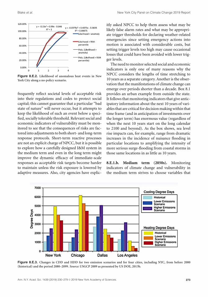
Blake et al. New York City Panel on Climate Change 2019 Report
Figure 8.E.2. Likelihood of anomalous heat events in NewYork City along a no-policy scenario.
frequently reflect societal levels of acceptable riskinto their regulations and codes to protect socialcapital; this cannot guarantee that a particular “badstate of nature” will never occur, but it attempts tokeep the likelihood of such an event below a speci-fied, socially tolerable threshold. Relevant social andeconomic indicators of vulnerability must be mon-itored to see that the consequences of risks are fac-tored into adjustments to both short- and long-termresponse protocols. Short-term reactive processesare not an explicit charge of NPCC, but it is possibleto explore how a carefully designed I&M system inthe medium term and even in the long term mightimprove the dynamic efficacy of immediate-scaleresponses as acceptable risk targets become harderto maintain unless the risk exposure is lowered byadaptive measures. Also, city agencies have explic-
itly asked NPCC to help them assess what may belikely false alarm rates and what may be appropri-ate trigger thresholds for declaring weather-relatedemergencies since setting emergency actions intomotion is associated with considerable costs, butsetting trigger levels too high may cause occasionallosses that could have been avoided with lower trig-ger levels.
The need to monitor selected social and economicindicators is only one of many reasons why theNPCC considers the lengths of time stretching to10 years as a separate category. Another is the obser-vation that the manifestations of climate change canemerge over periods shorter than a decade. Box 8.1provides an urban example from outside the state.It follows that monitoring indicators that give antic-ipatory information about the next 10 years of vari-ables that are critical for decision making within thattime frame (and in anticipation of investments overthe longer term) has enormous value (regardless ofwhen the next 10 years start on the long calendarto 2100 and beyond). As the box shows, sea levelrise impacts can, for example, range from dramaticincreases in the incidence of nuisance flooding inparticular locations to amplifying the intensity ofmore serious surge-flooding from coastal storms inthose same locations in as little as 10 years.
8.E.1.b. Medium term (2050s). Monitoringindicators of climate change and vulnerability inthe medium term strives to choose variables that
Figure 8.E.3. Changes in CDD and HDD for two emission scenarios and for four cities, including NYC, from before 2000(historical) and the period 2080–2099. Source: USGCP 2009 as presented by US DOE, 2013b.
273Ann. N.Y. Acad. Sci. 1439 (2019) 230–279 C© 2019 New York Academy of Sciences.

New York City Panel on Climate Change 2019 Report Blake et al.
Box 8.E.2. Heating degree days and cooling degree days
The definition of heating degree days (HDDs) and cooling degree days (CDDs) as referred to in Table 8.E.1and Table 8.E.2 is as follows: “Degree Days” are climate metrics that can be used to project the energy demandrequired for space heating and cooling as outdoor temperatures depart from a range of comfortabletemperatures. HDD and CDD are defined as the time-integrated difference (over a month or a year) betweenthe mean daily temperature and a reference temperature; for the latter 65°F (18 °C) is typically used in theUnited States. The monthly and total yearly HDDs and CDDs for New York City, as measured at La GuardiaAirport, are displayed in Table 8.E.1 and Table 8.E.2, respectively, for the period 2007 through 2017. “Normal”is defined as the 30-year degree-day average value for the period 1971–2000. Note: the lower the HDD, thewarmer the weather since less heating is needed; and the higher the CDD, the warmer the weather as morecooling is needed.
provide insight into which portion of the diverserange of possible long-term futures derived fromextensive scenario analysis is most likely, or mostextreme, or perhaps even most benign. The goal,here, is to identify and monitor indicators that serveas transparent harbingers of what should or shouldnot be anticipated for the most critical drivers offundamental risk analyses. Analyses can be targeted,for example, to inform the design and implementa-tion of protective measures and/or other transientprojects.
Monitoring selected indicators in the medium-term is, therefore, an exercise in looking fordetectable changes in variables that can beattributed to climate change and upon which one
can build robust triggers for anticipatory invest-ment decisions—decisions for protecting existingand designing new public and private infras-tructure as well as public and private property,more generally. The Preliminary Climate ResilienceDesign Guidelines issued in 2017 by the NYCMayor’s Office of Recovery and Resilience (ORR)provides guidance for choosing climate-resilientdesign parameters, approaches, and adjustmentsfor the useful life of assets (buildings, facilities,infrastructure); see this useful lifetime is oftenlonger than the formally assigned design lifetime.(http://www1.nyc.gov/assets/orr/images/content/header/ORR_ClimateResiliencyDesignGuidelines_PRELIMINARY_4_21_2017.pdf.
Table 8.E.1. HDD—monthly and yearly (“total”) heating degree days for NYC (La Guardia) 2007–2017
2017 2016 2015 2014 2013 2012 2011 2010 2009 2008 2007 Normal
January 780 903 1086 1123 899 846 1081 988 1114 848 806 1008
February 614 769 1136 938 851 680 794 871 780 810 981 861
March 738 499 835 866 755 438 714 520 713 683 682 713
April 246 357 344 412 366 294 354 219 360 321 421 392
May 122 145 53 88 128 69 114 82 111 148 75 136
June 16 2 35 0 4 11 4 0 27 0 3 16
July 0 0 0 0 0 0 0 0 0 0 0 1
August 0 0 0 0 0 0 0 0 0 0 6 1
September 10 5 3 14 31 9 19 0 23 15 5 40
October 76 161 217 166 172 173 223 163 256 252 91 249
November 378 352 579 577 591 383 461 395 547 530 524
December 759 435 752 826 681 662 923 868 802 808 836
Total 3978 4496 4938 4609 3792 4288 4227 4647 4426 4408 4777
Note: The HDD and CDD, when monitored over sufficiently long periods, can show climate trends, which apart from temporalmonthly or annual variability, shows an overall warming trend in the NYC area as demonstrated by Tables 8.4 and 8.5 and it does soin the context of energy needs for (less) heating needs in the winter and (more) cooling needs in the summer, over just this 11-yearperiod. The lower the HDD, the warmer is the weather.
274 Ann. N.Y. Acad. Sci. 1439 (2019) 230–279 C© 2019 New York Academy of Sciences.

Blake et al. New York City Panel on Climate Change 2019 Report
Table 8.E.2. CDD—monthly and yearly (“total”) cooling degree days for NYC (La Guardia) 2007–2017
2017 2016 2015 2014 2013 2012 2011 2010 2009 2008 2007 Normal
January 0 0 0 0 0 0 0 0 0 0 0 0
February 0 0 0 0 0 0 0 0 0 0 0 0
March 0 5 0 0 0 0 0 0 0 0 0 1
April 30 8 2 0 0 18 1 13 31 5 10 6
May 73 106 119 49 87 102 72 124 51 30 129 54
June 277 269 226 230 278 254 239 337 131 325 276 209
July 413 506 445 380 505 484 486 557 301 470 401 377
August 329 519 451 322 340 430 346 428 403 318 385 336
September 211 271 281 178 129 184 195 232 117 184 251 141
October 96 46 14 24 49 31 24 21 7 14 114 17
November 2 5 0 0 0 0 0 0 0 0 1
December 0 1 0 0 0 0 0 0 0 0 0
Total 1732 1544 1183 1388 1513 1363 1712 1041 1346 1566 1142
The key here can also be to identify indicators ofnear-term projections of climate change variablesthat effectively inform portraits of future conditionsthat are useful in designing responsive adaptationprojects. These are flexible adaptations that can, withsome notice, be adjusted over longer time framesthan those considered in the short and mediumterms. For example, the air-vents for the new railtunnel under the Hudson River must be locateddirectly over the tunnel on undeveloped property;there are only two locations that meet these criteria,and they are both near the shoreline on low landthat can flood. The tidal range of the Hudson in thearea is sensitive to sea level rise and thus increasingrisk as the tunnel matures through its 100+ year lifespan. Sea level rise poses a monitorable and mea-sureable hazard, notably as it contributes to stormtides, but the first iteration of the vents need not nec-essarily protect against the 2100 sea level. Design-ing vents to which additional height could easily beadded (as needed), that is, at as yet undeterminedtimes in the future (depending on the pace of sealevel rise, and/or changes in frequency/severity ofstorms), could be a solution. The indicators for suchprojects should monitor and measure more than sealevel rise; they should also be sensitive to satisfyingthe design and implementation needs of additionalprotective measures that solidify a long-term tran-sition to new and sustainably resilient public andprivate infrastructure and property.
Quoting another example, the post-Sandy SIRRReport proposed, as an interim adaptation option,
the installation of temporary, removable floodwallsin Red Hook, Brooklyn (SIRR, 2013, Initiative 23). Itmay be desirable to have an indicator that shows theannual number of deployments of such removableflood protection devices, and from that indicatorinfers the circumstances under which they becomeunreliable protective devices, or when their increas-ingly frequent deployment becomes operationallytoo costly. Collecting this information could informa warning or monitoring mechanism designed toindicate when a longer term, permanent solutionneeds to be planned, designed, financed, and putinto place.
8.E.1.c. Long term (2080s, 2100, and beyond).Long-term I&M anticipates, through forward-looking risk analyses across diverse scenarios,indicators that would (1) inform long-term invest-ments; (2) inform the need to provide dynamicadaptive hedging strategies to protect those invest-ments; and (3) consider changes in landuse andzoning, including, where appropriate, relocationto higher ground. Care must be taken, here, inconsidering the interdependencies across differenttypes of infrastructure, because the most effectivelong-term indicators for one type of infrastructuremay not include all of the indicators required andlisted for another that in turn may adversely affectthe initial infrastructure. The key to (1) is to identifyprojections of climate change indicators acrossmultiple models and distributions so that they canbe used in the initial planning and implementation
275Ann. N.Y. Acad. Sci. 1439 (2019) 230–279 C© 2019 New York Academy of Sciences.
New York City Panel on Climate Change 2019 Report Blake et al.
stages of long-term infrastructure and propertyinvestments. For example, this may include optionsto finance buy-outs of flood-prone communitiesand provide assistance for their strategic relocation.The key to (2) is to identify sources of vulnera-bility for the investments along these projections,adaptive responses that could ameliorate thatvulnerability, and indicators that could be tiedto decision triggers as the future unfolds. Thekey to (3) is to find indicators and appropriatemetrics that would show that engineered protectionand/or accommodation of certain assets becomesineffective, whether physically or economically,with time (i.e., due to continuing sea level rise); andthat a relocation to higher ground (if and whereavailable) becomes either unavoidable or econom-ically advantageous. Such relocations may hingeon changes in land-use and/or zoning, and settingaside the necessary finance mechanisms. All ofthese measures require considerable lead times, andany indicators that serve as triggers need to accountfor such long lead times. For instance, London’sprotective Thames Barriers are assessed in the faceof sea level rise to become progressively ineffectiveby mid-century. The responsible agencies havedeveloped already a plan for their substitutionwith a new comprehensive flood managementplan named Thames Estuary 2100 (TE2100;https://www.gov.uk/government/publications/thames-estuary-2100-te2100).
8.E.2. Time scales calibrated from 2100 totoday
8.E.2.a. The long term (2080s, 2100, andbeyond). Notwithstanding that the currentpolicy-making focus on looking historically fromtoday, it is essential that indicators be calibrated toprojections of the future, as well; they need to beinformed by the limitations of scientific knowledgethat have focused attention on the year 2100 and notthe decades that stretch from now until then.
We use Figure 8.E.1, extracted from Fawcett et al.(2015), to anchor this perspective in contempo-rary research. Figure 8.E.1.a (left) depicts projec-tions of future energy and industrial CO2 emissionsfrom multiple models under five alternative policyregimes: a no policy reference; a reference low policyalternative; a continuation of the Paris Accord past2030, a transition from the Paris Accord to a moreaggressive global policy in 2030, and an even more
aggressive policy stance that keeps the likelihood ofexceeding 2 °C by 2100 below 50%. These scenariosare described in the IPCC AR5 Scenario Data Base(http://bit.ly/AR5Scenarios).
Figure 8.E.1.b (right) reflects probability dis-tributions of temperature increases through 2100for the five policy alternatives. Each distribution isdifferent, and each is supported by subsets of emis-sions scenarios and associated temperature scenar-ios from roughly 2010. These subsets are typicallycharacterized by similarities in the specification ofsome critical drivers of climate change (notablyeconomic growth, economic diversification acrossmultiple sectors, trade interdependency, and energyintensity across fossil and nonfossil sources) and thesensitivity of climate impacts to those drivers (notonly temperature change). Together, they dividea complicated future into five more manageablecohorts of 80-year emissions trajectories that canbe differentiated one from another not only by dif-ferent policy regimes, but also by careful accountingof differences in the specifications of their under-lying drivers and assumed sensitivities. From there,a wide range of other manifestations that are sum-marized in the IPCC “Reasons for Concern” (IPCC,2014c) can be attached to each cohort—for exam-ple, trajectories of extreme weather, sea level riseand storm surge, increases in average temperature,heat waves, cold snaps, extreme winds, heavy rain-fall, inland flooding—the climate hazards that havealready been identified above for the five key sectors.
8.E.2.b. The medium term. Figure 8.E.1. is allabout the long term, but the long term is nothingmore than a series of distinct medium and shortterms that follow one after another. Moreover, thepattern of short- and medium-term decision peri-ods marches forward as time passes; that is, 2060is now part of the long-term horizon, but it willbe in a medium-term horizon in 2030 and a short-term horizon in 2050. These two simple observa-tions of decision-term interdependence illuminatean advantage of approaching the time dimension ofthe indicator/monitoring issue from the long termvery clear. Long-term trajectories characterized byspecifications of underlying driving and sensitiv-ity parameters of manageable cohorts necessarilypass through the 10- and 30-year thresholds for theother time periods, starting now and moving intothe future.
276 Ann. N.Y. Acad. Sci. 1439 (2019) 230–279 C© 2019 New York Academy of Sciences.

Blake et al. New York City Panel on Climate Change 2019 Report
Recent work in support of the Special Report onLimiting Temperature to an increase of 1.5 degreesCentigrade (2.7 degrees Fahrenheit) that is underpreparation by the Intergovernmental Panel onClimate Change offers some encouraging context.Box 8.E.1 is an example from Yohe (2017); indeed,it offers insight into the incidence of extreme heat(a critical climate driver of concern for all five of theNYC key sectors) in decadal increments along twomitigation scenarios as well as a business as usualfuture— all portrayed in Figure 8.E.1 above fromFawcett et al. (2015). The decadal increments, infact, inform not only the medium term, but also theshort term and how the planet will track to reachthe 2100 benchmarks.
8.E.2.c. The short term (2020s). Turning finallyto the immediate time scale of New York City rule-of-thumb responses to observed climate-relatedthreats. Some of the indicators that are already beingmonitored to inform the very short-term responseswill likely match (or at least correlate well statisti-cally) to at least some of the drivers of the longerterms described above. That is to say, the sensi-tivities of these “rule of thumb” indicators to cli-mate change can be calibrated from historical data(e.g., number of heat waves per year with 3 con-secutive days with average temperatures at or above95 degrees Fahrenheit), and a link to the drivers ofprojected climate change can thereby be established.This link is, perhaps, one new step in the process ofanchoring these indicators with characterizationsof current and past conditions (including distribu-tions of the likelihood of crossing some thresholdof tolerable risk to which the city must respond). Itis also the foundation of a process that can providethe city with insight into how the efficacy of theirrules of thumb can be expected to evolve over timealong the early parts of the alternative cohorts oflong-term scenarios—valuable information in anyattempt to estimate when it might be prudent toamend existing decision rules.
Melding the forward and backward perspectives,the changes in HDD and CDD have been projectedfor the period 2080–2099 for four major cities inthe United States, located in four different climatezones, for a low emission scenario (B1) and a veryhigh emissions scenario (A1FI), in the IPCC ter-minology. Note that the four cities, NYC, Chicago,Dallas, and Los Angeles, are located in four different
climate zones which lead to different patterns, spa-tially and temporally, for the changes in HDD andCDD, as demonstrated in Figure 8.E.3. The higherthe CDD, the warmer is the weather.
Appendix 8.F. Interdependency indicators
A theoretical framework that organizes thoughtsaround sector interdependencies is shown inFigure 8.F.1. In the figure, indicators for the energysector (totaling n in number) are reflected as {E1,. . . . En} of which the first “EEa” are specific to energyand the remaining (n–EEa –1) are shared with thetransportation sector. Indicators for the transporta-tion sector (totaling m in number) are reflected as{T1, . . . . Tm} of which the first “TTa” are specificto transportation and the remaining (m–TTa–1) areshared with the energy sector. That is to say, sets{EEa+1, . . . . En} and {TTa+1, . . . . Tm} are the collec-tions of the same indicators; they live in the intersec-tion of the energy and transportation ovals. Otherinterdependence indicators are possible; they aredistinct and indicated outside the intersection by{I1, . . . . IO}.
8.F.1. Recovery ratios (ratios of recovery rates).A common measure of interdependence and depen-dence is recovery rate. The indicator can beexpressed as the ratio of the rate of recovery of asecondary-dependent infrastructure to the recov-ery of a primary or initial infrastructure that repre-sents a first stage. This can then cycle through manystages advancing over time and in some cases, overmultiple-dependent infrastructure systems.
Example: Using electric power as a starting point,a first-stage recovery ratio for NYC during the 2003blackout, linking electric power and transit, is:
The time Ti it takes for an infrastructure depen-dent upon electric power to recover divided bythe time Te it takes for electric power to recover.This is illustrated for transit component recoveryin NYC following the 2003 blackout (Zimmermanand Restrepo, 2006): Ti/Te, where Ti is the timeto recover for a given infrastructure, and Te isthe time for electric power to recover. The resultsfor NYC transportation systems were as follows(Zimmerman and Restrepo, 2006):
For NYCT subway signals, the ratio is 1.3.For NYC DOT Street Traffic signals, the ratio
is 2.6.
277Ann. N.Y. Acad. Sci. 1439 (2019) 230–279 C© 2019 New York Academy of Sciences.

New York City Panel on Climate Change 2019 Report Blake et al.
Figure 8.F.1. A schematic diagram of indicators for the energy and transportation sectors and possible interdependences.
The electric power to transportation linkage canbecome an interdependency when a failure of atransportation system can prevent electric powerrepair workers from getting to the damaged electricpower sites in order to repair them.
Recovery times have been computed for sin-gle infrastructures following major weather events.For example for electric power following hurri-canes, recovery displays distinctly different patternsfor different weather events and energy compo-nents. These recovery footprints, specified at thelevel of energy components, were developed forexample for hurricanes by the U.S. DOE (DOE,2009, 2013a), and are a first step in formulatinginterdependencies.
Transit recovery following Hurricane Sandy hasbeen documented by the MTA for each of its25 NYCT subway lines, and appears in a cou-ple of publications (Zimmerman, 2014; Kaufmanet al., 2012), and when connected to electric poweroutages become dependencies and interdepen-dencies.
8.F.2. Usage rates and ratios. The extent towhich one infrastructure uses the outputs of anotherand in turn provides inputs to the other is a measureof interdependency. These relationships at infras-tructure sector levels are often displayed as “Sankey”diagrams. An example is the flow of energy sourcesto different sectors of the economy (USDOE, 2016;US EIA, 2013).
Across different infrastructure sectors, the U.S.Department of Energy (2014), for example, has an
extensive set of quantified measures of use of waterby energy and energy by water disaggregated byenergy production technology.
U.S. Department of Energy (DOE) (2014). Thewater-energy nexus: Challenges and opportunities,Washington, DC.
For New York City, another example of usageacross infrastructures exists for water and tran-sit. For example, data exist (MTA, 2008) for theusage of water by MTA transit systems. For 2006,the MTA Commission indicated that approximately2.6 billion gallons per year of water was used forpotable purposes and another 156 million gallonsper year was used for wash operations. Of thosetotals, NYC Transit used 1.9 billion or almost threequarters of the potable water and over 80% of theMTA wash water volumes used in that year (bus andsubways combined).
8.F.3. Network characteristics. Measures ofnetwork properties are commonly applied to infras-tructure components and can be extended tointerdependencies.
These network measures include, for example,“betweenness” and “centrality” that measure thecloseness of portions or components of systems toone another as well as the density (Wasserman andFaust, 1994).
Appendix 8.G. Credit rating supplementalmaterial
The text below highlights factors and rev-enue sources that could be sensitive to large
278 Ann. N.Y. Acad. Sci. 1439 (2019) 230–279 C© 2019 New York Academy of Sciences.

Blake et al. New York City Panel on Climate Change 2019 Report
extreme weather events that could have beenattributed to anthropogenic climate change, orat least, the weather manifestations of a dynamicclimate. It turns out that they are not. Thepositive characteristics for NYC have sustainedan AA rating through Hurricane Sandy andthe financial crisis that began in 2008 (Source:http://www.ott.ct.gov/debt_creditratingprocess.html).;the text in bold italics highlights positive char-acteristics for NYC that have sustained an AArating through Hurricane Sandy and the financialcrisis).
(Source: http://www.ott.ct.gov/debt_creditratingprocess.html).Criteria for credit ratings:
AAA (Aaa)Bonds rated AAA have the highest ratings
assigned by rating agencies. They carry the smallestdegree of investment risk. Issuer’s capacity to payinterest and principal is extremely strong.
AA (Aa)Bonds rated AA are judged to be of high quality
by all standards. They differ from the highest rated(AAA) bonds only in a small degree. Issuer’s capacityto pay interest and principal is very strong (Optionalrelative standing within a rating category:+/– (FitchRatings, Kroll, Standard and Poor’s Global Ratings);1,2,3 (Moody’s)).
ABonds rated A have strong capacity to pay inter-
est and repay principal although they are somewhatmore susceptible to the adverse effects of changes incircumstances and economic conditions than bondsin higher rated categories. (Optional relative stand-ing within a rating category: +/– (Fitch Ratings,Kroll, Standard and Poor’s Global Ratings); 1,2,3(Moody’s)).
BBB (Baa)Bonds rated (BBB) are considered medium-grade
obligations. They are neither highly protected norpoorly secured. Interest payments and principalsecurity appear adequate for the present but cer-tain protective elements may be lacking or unreliableover any length of time. These bonds lack outstand-ing investment characteristics and have speculativecharacteristics as well (Optional relative standingwithin a rating category: +/– (Fitch Ratings, Stan-dard and Poor’s Global Ratings);
1,2,3 (Moody’s)).
More detailed elements involved in determining acredit rating
Economic FactorsEvaluation of historical and current economic
factors—climatic factors projected forward could playa role, here.
Economic diversityResponse to business cycles—and climate cycles.Economic restructuringAssessing the quality of life in the given areaDebt/issue structureEconomic feasibility and need for projectLength of bonds’ maturity, short-term debt
financingPledged security and other bondholder
protectionsFuturistic outlook: capital improvement planFinancial factorsSufficient resources accumulated to meet unforeseen
contingencies and liquidity requirements—climatevulnerability, especially if repeated frequently, over ashort period of time.
Ongoing operations are financed with recurringrevenues
Prudent investing of cash balancesAbility to meet expenditures within economic
baseManagement/structural factorsOrganization of government and managementTaxes and tax limitsClear delineation of financial and budgetary
responsibilitiesContinuing disclosureExpanded analytical topics—investment policies
and practicesPortfolio composition-credit risk, diversification,
and market riskLeverage-increase of assets to enhance yieldLiquidity management-portfolio maturity pro-
file that matches cash flowInfrastructure needs—significant investment to
fund adaptive infrastructure could create fiscal stress.Willingness to payPortfolio composition-credit risk, diversification,
and market riskLeverage-increase of assets to enhance yieldLiquidity management-portfolio maturity profile
that matches cash flowInfrastructure needs.
279Ann. N.Y. Acad. Sci. 1439 (2019) 230–279 C© 2019 New York Academy of Sciences.