new york city department of environmental … new york city department of environmental protection...
TRANSCRIPT

i
New York City Department of Environmental Protection
Bureau of Water Supply
Multi-Tiered Water Quality Modeling Program
Annual Status Report
March 2016
Prepared in accordance with Section 5.2 of the NYSDOH
Revised 2007 Filtration Avoidance Determination
Prepared by: DEP, Bureau of Water Supply
Emily Lloyd, Commissioner Paul V. Rush, P.E., Deputy Commissioner

2015 Water Quality Modeling Annual Report
ii

Table of Contents
i
Table of Contents
List of Figures ................................................................................................................................ iv
List of Tables .................................................................................................................................. x
Acknowledgements ....................................................................................................................... xii
Executive Summary ..................................................................................................................... xiii
1. Introduction ............................................................................................................................. 1
2. Use of Models for Support of Operational Decisions ............................................................. 5
3. Modeling Applications of Climate Change Impacts ............................................................... 7
3.1. Climate Change Integrated Modeling Project .................................................................. 7
3.2. Evaluation of Stochastic Weather Generators (SWGs) for use in Simulating
Precipitation ................................................................................................................................ 7
3.2.1. Introduction ............................................................................................................... 7
3.2.2. Data ........................................................................................................................... 9
3.2.3. Stochastic Weather Generators ............................................................................... 11
3.2.4. Implementation of SWGs ....................................................................................... 12
3.2.5. Statistical Evaluation of SWGs for daily precipitation characteristic .................... 15
3.2.6. Performance of SWGs for Extreme Precipitation Events ....................................... 21
3.2.7. Discussion ............................................................................................................... 25
3.2.8. Conclusions and Future Work ................................................................................ 26
4. Model Development and Applications ................................................................................. 29
4.1. Realistically predicting saturation-excess runoff with SWAT-Hillslope ....................... 29
4.1.1. Introduction ............................................................................................................. 29
4.1.2. Methodology ........................................................................................................... 30
4.1.3. Results ..................................................................................................................... 42
4.1.4. Discussion ............................................................................................................... 49
4.1.5. Conclusions ............................................................................................................. 53
4.2. Application of the General Lake Model (GLM) to Cannonsville and Neversink
Reservoirs ................................................................................................................................. 54
4.2.1. Methods................................................................................................................... 55

2015 Water Quality Modeling Annual Report
ii
4.2.2. Results and Discussion ........................................................................................... 67
4.3. Development and Testing of a Probabilistic Turbidity Model for Rondout Reservoir .. 77
4.3.1. Background ............................................................................................................. 77
4.3.2. Approach ................................................................................................................. 77
4.3.3. Model Specifications for an Example Application ................................................. 80
4.3.4. Results and Discussion ........................................................................................... 81
4.3.5. Future Work ............................................................................................................ 87
4.4. Simulation of the Impact of Drawdown of Cannonsville Reservoir on Turbidity in
Rondout Reservoir .................................................................................................................... 88
4.5. Ecohydrologic Modeling ................................................................................................ 97
4.5.1. Introduction ............................................................................................................. 97
4.5.2. Study sites ............................................................................................................... 99
4.5.3. RHESSys model.................................................................................................... 101
4.5.4. Estimates of vegetation indices using Landsat TM imagery ................................ 102
4.5.5. RHESSys calibration ............................................................................................ 104
4.5.6. Conclusions and future plans ................................................................................ 107
5. Data Analysis to Support Modeling .................................................................................... 109
5.1. West of Hudson Reservoir Water Budgets, 2000-2015 ............................................... 109
5.2. Hydraulic Residence Time in West of Hudson Reservoirs .......................................... 120
6. Model Data Acquisition and Organization ......................................................................... 127
6.1. GIS Data Development for Modeling .......................................................................... 127
6.1.1. Water Quality Monitoring Sites ............................................................................ 127
6.1.2. Support for modeling projects .............................................................................. 127
6.2. Ongoing Modeling/GIS Projects .................................................................................. 128
6.2.1. Reservoir Bathymetry Surveys ............................................................................. 128
6.2.2. Modeling Database Design ................................................................................... 129
6.3. Time Series Data Development.................................................................................... 129
7. Modeling Program Collaboration ....................................................................................... 133
7.1. Water Research Foundation Project 4422 – Advanced Techniques for Monitoring
Changes in NOM and Controlling DBPs Under Dynamic Weather Conditions .................... 133

Table of Contents
iii
7.2. Water Research Foundation Project 4590 - Wildfire Impacts on Drinking Water
Treatment Process Performance: Development of Evaluation Protocols and Management
Practices .................................................................................................................................. 134
7.3. Water Utility Climate Alliance (WUCA)..................................................................... 134
7.4. Global Lake Ecological Observatory Network (GLEON) ........................................... 135
7.5. NYCDEP – City University of New York (CUNY) Modeling Program ..................... 138
8. Modeling Program Scientific Papers and Presentations ..................................................... 139
8.1. Published Scientific Papers .......................................................................................... 139
8.2. Conference Presentations ............................................................................................. 140
9. References ........................................................................................................................... 151

2015 Water Quality Modeling Annual Report
iv
List of Figures
Figure 1.1. Overview of DEP’s Water Quality Modeling Program. ...............................................2
Figure 3.1. Precipitation gage stations over the study region. .......................................................10
Figure 3.2. Flow chart showing the methodology of calibration of SWG. ....................................14
Figure 3.3. Mean and standard deviation of the observed and generated counter part of wet
days per month from MC1, MC2 and MC3. ..........................................................16
Figure 3.4. Mean, standard deviation and extreme (Q99) of wet spells of the observed and
generated counterpart from MC1, MC2 and MC3.................................................17
Figure 3.5. Mean, standard deviation and extreme (Q99) of dry spells of the observed and
generated counterpart from MC1, MC2 and MC3.................................................18
Figure 3.6. Mean, standard deviation and skewness coefficients of observed and generated
daily precipitations from seven models (EXP, GAM, SN, MEXP, EXPP, k-
NN and PN)............................................................................................................20
Figure 3.7. Probability distribution functions of observed and generated daily
precipitations from seven models (EXP, GAM, SN, MEXP, EXPP, k-NN
and PN) for Ashokan watersheds. ..........................................................................21
Figure 3.8. RX1day, RX5day, R95p and R99p of observed and generated daily
precipitations from seven models (EXP, GAM, SN, MEXP, EXPP, k-NN
and PN). .................................................................................................................23
Figure 3.9. Annual maximum daily precipitation levels at the 50, 75 and 100 year return
periods of observed and generated daily precipitations from seven models
(EXP, GAM, SN, MEXP, EXPP, k-NN and PN). The error bars refers the
95% confidence interval for each return levels. .....................................................24
Figure 4.1. Examples of storage capacity distribution of a watershed: (a) watershed
dominated by dry areas, and (b) watershed dominated by perennial
wetlands. ................................................................................................................32
Figure 4.2. Difference in hydrological processes between the original SWAT and SWAT-
Hillslope .................................................................................................................33
Figure 4.3. Town Brook watershed, Delaware County, New York ...............................................35
Figure 4.4. Relationship between topographic index (λ) and probability of saturation (Psat
)
in April, August and October (Agnew et al., 2006). The symbol are the

List of Figures
v
average Psat
for corresponding λ. The dashed lines correspond to 25th and
75th percentiles. ......................................................................................................36
Figure 4.5. Wetness map for the Town Brook watershed..............................................................37
Figure 4.6. Soil types in the Town Brook watershed (Source: SSURGO soil database) ..............38
Figure 4.7. Meteorological grid points used for the Town Brook watershed ................................40
Figure 4.8. Comparison of simulated daily and monthly discharge values between SWAT-
Hillslope, SWAT2012 and measured data .............................................................45
Figure 4.9. Scatter plot of daily and monthly simulated flow by SWAT-HS and SWAT2012
versus observed flow..............................................................................................46
Figure 4.10. Time series of flow components simulated by SWAT-Hillslope in comparison
with SWAT2012 ....................................................................................................47
Figure 4.11. Spatial distribution of annual surface runoff simulated by SWAT-Hillslope
and SWAT2012. ....................................................................................................48
Figure 4.12. Saturated areas simulated by SWAT-Hillslope compared with observations. ..........50
Figure 4.13 Idealized hillslope profile according to statistical dynamic approach. Water
table saturates at location 1, intersects the root zone at location 2, and is
below the root zone at location 3. ..........................................................................51
Figure 4.14. Water capacity distribution functions for two different topographic regimes.
a) with limited benches and floodplains, limited maximum extent of VSAs,
and characterized by a TWI storage capacity distribution. b) catchment with
extensive floodplains, extensive extent of VSAs, and characterized by a
pareto distribution with b>1 (Moore 2007). ..........................................................53
Figure 4.15. Land use within the watersheds of (a) Cannonsville Reservoir, and (b)
Neversink Reservoir...............................................................................................55
Figure 4.16. Bathymetric curves for Cannonsville Reservoir. .......................................................56
Figure 4.17. Bathymetric curves for Neversink Reservoir. ...........................................................56
Figure 4.18. Meteorological data for Cannonsville Reservoir, 2007-08. ......................................60
Figure 4.19. Meteorological data for Neversink Reservoir, 2007-08. ...........................................62
Figure 4.20. Components of the water budget for Cannonsville Reservoir, 2007-2008: (a)
inflows, and (b) outflows. ......................................................................................63
2015 Water Quality Modeling Annual Report
vi
Figure 4.21. Components of the water budget for Neversink Reservoir 2007-2008: (a)
inflows, and (b) outflows. ......................................................................................64
Figure 4.22. Inflow temperatures of Cannonsville Reservoir (a) and Neversink Reservoir
(b). ..........................................................................................................................65
Figure 4.23. Simulated water level (grey) and observed water level (black) of Cannonsville
Reservoir (dash line is the spillway elevation). .....................................................67
Figure 4.24. Simulated water level (grey) and observed water level (black) of Neversink
Reservoir (dash line is the spillway elevation). .....................................................68
Figure 4.25. GLM simulated temperature in Cannonsville Reservoir. ..........................................69
Figure 4.26. GLM simulated temperature in Neversink Reservoir. ..............................................69
Figure 4.27. GLM simulated temperature for the surface water layer (a) and the bottom
water layer (b) in Cannonsville Reservoir. ............................................................70
Figure 4.28. GLM simulated temperature for the surface water layer (a) and the bottom
water layer (b) in Neversink Reservoir. .................................................................70
Figure 4.29. Simulated temperature profiles and field data at Site 4 in Cannonsville
Reservoir in 2007. ..................................................................................................72
Figure 4.30. Simulated temperature profiles and field data at all sites of Cannonsville
Reservoir in 2007. ..................................................................................................72
Figure 4.31. Simulated temperature profiles and field data at all sites of Cannonsville
Reservoir in 2008. ..................................................................................................73
Figure 4.32. Simulated temperature profiles and field data at Site 1 in Neversink Reservoir
in 2007. ..................................................................................................................74
Figure 4.33. Simulated temperature profiles and field data at all sites of Neversink
Reservoir in 2007. ..................................................................................................74
Figure 4.34. Simulated temperature profiles and field data at all sites of Neversink for 2008.
................................................................................................................................75
Figure 4.35. Simulated withdrawal temperatures (lines) and observed withdrawal
temperatures (circles) of Cannonsville Reservoir: (a) 2007, and (b) 2008. ...........76
Figure 4.36. Simulated withdrawal temperatures (lines) and observed withdrawal
temperatures (circles) of Neversink Reservoir: (a) 2007, and (b) 2008.. ..............76

List of Figures
vii
Figure 4.37. Conceptual framework of a probabilistic turbidity model for Rondout
Reservoir. (NOAA: National Oceanic and Atmospheric Administration,
HEFS: Hydrologic Ensemble Forecast System, OST: Operations Support
Tool) .......................................................................................................................78
Figure 4.38. CE-QUAL-W2 model segmentation of Rondout Reservoir, including
monitoring location on the tributaries, and in the reservoir. Inputs from the
upstream Cannonsville, Pepacton, and Neversink reservoirs are indicated
by WBDT, EDT, and NST, respectively. ..............................................................79
Figure 4.39. Ensemble forecast of Rondout Creek inflow for 11/13/2015–12/1/2015. Forty
seven individual traces, median, 10th and 90th percentile traces are shown
along with the observations from USGS. ..............................................................82
Figure 4.40. Ensemble forecast of turbidity in the withdrawal from Rondout Reservoir
(RDRR) for 11/13/2015–12/1/2015. One Hundred of the 1175 individual
traces, median, 10th and 90th percentile traces are shown. .....................................83
Figure 4.41. Predictions of turbidity in the withdrawal from Rondout Reservoir for
11/13/2015–12/1/2015 interval. Predicted median, 10th and 90th percentiles
values are compared with historical median values and actual observations.
................................................................................................................................83
Figure 4.42. Predictions of turbidity in the withdrawal from Rondout Reservoir for
11/13/2015–12/1/2015 interval. Percentages of simulation traces that
predict turbidity less than the specified levels (0.5, 0.75, 1, 2, and 2.5 NTU)
and probability of exceedance (= 100 − percent of traces less than) are
shown. ....................................................................................................................84
Figure 4.43. Predictions of turbidity in the withdrawal from Rondout Reservoir for
11/13/2015–12/1/2015 interval. Average number and percentages of the
days the turbidity exceeds the specified levels (0.5, 0.75, 1, 2, and 2.5 NTU).
................................................................................................................................85
Figure 4.44. Time series of standard deviation of withdrawal turbidity computed from
multiple traces of predictions due to variations in meteorology and
hydrology. ..............................................................................................................86
Figure 4.45. Predictions of median turbidity in the withdrawal from Rondout Reservoir for
11/13/2015–12/1/2015 interval. Median values as computed from 1175
traces are compared with values from 100 randomly selected traces in 25 of
such sampling experiments. ...................................................................................87
Figure 4.46. Cannonsville water surface elevation, observations and OST forecast, July
through September, 2015. ......................................................................................89

2015 Water Quality Modeling Annual Report
viii
Figure 4.47. Frequency of occurrence of Cannonsville water surface elevation. ..........................89
Figure 4.48. Statistics of Cannonsville withdrawal turbidity as a function of reservoir
drawdown. ..............................................................................................................90
Figure 4.49. Forecast of Cannonsville withdrawal turbidity for the entire drawdown period,
August and September, 2015, and measurements in July 2015. ............................92
Figure 4.50. Forecasts of inflows to Rondout from upstream reservoirs for the August-
September drawdown period, and the Rondout Creek hydrograph for
August-September 2012.........................................................................................93
Figure 4.51. Observed and assumed turbidity in the Pepacton and Neversink inflows to
Rondout for August-September, 2015. ..................................................................93
Figure 4.52. Temperatures of the inflows to Rondout for August-September 2015 period
used in the model forecast. Cannonsville temperature determined from 1D
hydrothermal model based on OST forecast of inflow and outflow.
Pepacton and Neversink temperatures are average historical values, while
Rondout Creek temperature is the observed time series for 2012. ........................94
Figure 4.53. Predicted turbidity in the withdrawal from Rondout Reservoir during the
period of drawdown of Cannonsville Reservoir. ...................................................95
Figure 4.54. Actual drawdown of Cannonsville Reservoir, and July 29 OST forecast, for
period July 8 through September 30, 2015. ...........................................................96
Figure 4.55. The framework for studying the impact of disturbance on ecohydrologic
processes using RHESSys......................................................................................98
Figure 4.56. The study sites: (a) Neversink, (b) Biscuit Brook, and (c) Shelter Creek. ..............100
Figure 4.57. The Shelter Creek watershed with different forest harvest regimes. .......................101
Figure 4.58. Derived vegetation indices using Landsat-TM: (a) SR, (b) EVI, (c) NDVI, (d)
LAI using the calibrated equation (Hwang, unpublished data), (e) ISR, and
(f) LAI using the calibrated equation (Fernandes et al., 2003). ...........................103
Figure 4.59. Streamflow calibration for Shelter Creek and Biscuit Brook watershed: (a)
Shelter Creek watershed, and (b) Biscuit Brook watershed ................................106
Figure 5.1. Example of water budget calculation for Cannonsville for Feb. 21 to March 20,
2000: (a) components of the budget calculation, and (b) resulting error in
water surface elevation. .......................................................................................114
Figure 5.2. Cannonsville water budget results, 2015: (a) error in predicted water surface
elevation, and (b) gaged and ungaged inflows. ....................................................116

List of Figures
ix
Figure 5.3. Neversink water budget results, 2015: (a) error in predicted water surface
elevation, and (b) gaged and ungaged inflows. ....................................................117
Figure 5.4. Pepacton water budget results, 2015: (a) error in predicted water surface
elevation, and (b) gaged and ungaged inflows. ....................................................118
Figure 5.5. Rondout water budget results, 2015: (a) error in predicted water surface
elevation, and (b) gaged and ungaged inflows. ....................................................119
Figure 5.6. Typical or expected observation of dye tracer concentration in a reservoir
outflow in response to a quick release of tracer in a reservoir inflow. ................121
Figure 5.7. Storage in Catskill System Reservoirs, 1966 through 2015. .....................................123
Figure 5.8. Storage in Delaware System Reservoirs, 1966 through 2015. ..................................123
Figure 5.9. Reservoir outflow for Catskill system reservoirs, 1966 through 2015. .....................124
Figure 5.10. Reservoir outflow for Delaware system reservoirs, 1966 through 2015. ................124
Figure 5.11. Hydraulic residence time for Catskill System Reservoirs, 1966 through 2015.
..............................................................................................................................125
Figure 5.12. Hydraulic residence time for Delaware system reservoirs, 1966-2015. ..................125

2015 Water Quality Modeling Annual Report
x
List of Tables
Table 2.1. List of modeling analyses performed during the reporting period (January 1–
December 31, 2015) including descriptions of each analysis. .................................5
Table 3.1. Description of the nearest stations and associated weights for estimating
weighted mean precipitation for each of WOH watersheds ..................................10
Table 3.2. Description of some popular SWG with their precipitation occurrence and
amount components and respective reference. ......................................................13
Table 3.3. Seven models evaluated for generating daily precipitation amounts. ..........................14
Table 4.1. New parameters added to SWAT-Hillslope .................................................................34
Table 4.2. Classification of wetness classes for the Town Brook watershed. ...............................37
Table 4.3. Land use types in the Town Brook watershed ..............................................................39
Table 4.4. Parameters for calibration using Monte Carlo sampling method .................................43
Table 4.5. Performance criteria for SWAT-Hillslope in daily and monthly time step ..................44
Table 4.6. Spillway and Intake Elevations of Cannonsville Reservoir and Neversink
Reservoir. ...............................................................................................................58
Table 4.7. The simulation period for Cannonsville Reservoir and Neversink Reservoir. .............65
Table 4.8. GLM hydrothermal model coefficients that were adjusted during model
calibration. .............................................................................................................66
Table 4.9. The average root mean square error (RMSE) in predicted water column
temperatures (oC). ..................................................................................................71
Table 4.10. Specifications of operations of upstream reservoirs for the forecast interval of
11/13/2015–12/1/2015. ..........................................................................................81
Table 4.11. Observed temperature and turbidity depth profiles at sites 1, 2, and 3 in
Rondout Reservoir on 11/10/2015. ........................................................................81
Table 4.12. Watershed descriptions .............................................................................................100
Table 4.13. Shelter Creek watersheds with different forest harvest regimes...............................101
Table 4.14. Accuracy of Streamflow predictions for the Shelter Creek Watershed and the
Biscuit Brook watershed ......................................................................................107

List of Tables
xi
Table 5.1. U.S. Geological Survey (USGS) stream gaging and reservoir elevation stations
in the West of Hudson reservoirs. Stream gaging stations that are upstream
of other stations are not included. USGS gage remarks refer to accuracy of
stream gaging observations. .................................................................................110
Table 5.2 Descriptors of accuracy of USGS streamflow measurements (included in USGS
documents in “Remarks” section). .......................................................................111
Table 5.3. Annual water balance calculations for Cannonsville Reservoir, 2000 through
2015. Change in storage over the year and total annual inflow and outflow
volumes are in billion gallons (BG). ....................................................................116
Table 5.4. Annual water balance calculations for Neversink Reservoir, 2000 through 2015.
Change in storage over the year and total annual inflow and outflow
volumes in billion gallons (BG). ..........................................................................117
Table 5.5. Annual water balance calculations for Pepacton Reservoir, 2000 through 2015.
Change in storage over the year and total annual inflow and outflow
volumes in billion gallons (BG). ..........................................................................118
Table 5.6. Annual water balance calculations for Rondout Reservoir, 2000 through 2015.
Change in storage over the year and total annual inflow and outflow
volumes in billion gallons (BG). ..........................................................................119
Table 5.7. Comparison of computed ungaged inflow as a percentage of total (gaged plus
ungaged) inflow for the 16-year period, and the ungaged watershed area as
a percentage of the total (gaged plus ungaged) watershed area. ..........................120
Table 5.8. Statistics for hydraulic residence time for Catskill and Delaware system
reservoirs, 1966 through 2015. Mean and standard deviation in days. ...............122
Table 6.1. Inventory of GIS data used in water quality modeling. ..............................................128
Table 6.2. Inventory of time-series data used for watershed modeling. ......................................130
Table 6.3. Inventory of time-series data used for reservoir modeling. ........................................131

2015 Water Quality Modeling Annual Report
xii
Acknowledgements
This report was produced by the Water Quality Modeling group of Water Quality Science and
Research (WQSR), Directorate of Water Quality, in the Bureau of Water Supply at DEP.
During 2015, the Water Quality Modeling group was fortunate to have the services of 4 post-
doctoral researchers who are employed by the City University of New York (CUNY), and
worked day-to-day as a part of the Water Quality Modeling Group under contract with DEP (see
Section 7.5). These individuals, and the report sections which they authored, are: Nachiketa
Acharya, Ph.D. (Section 3.2), Linh Hoang, Ph.D. (Section 4.1), Yu Li, Ph.D. (Section 4.2), and
Kyongho Son, Ph.D. (Section 4.5). These researchers are supported by the following faculty
advisors: Allan Frei, Ph.D. (Hunter College, CUNY), Tammo Steenhuis, Ph.D. (Cornell
University), Paul Hanson, Ph.D. (University of Wisconsin), and Larry Band, Ph.D. (University
of North Carolina).
Rakesh Gelda, Ph.D., Research Scientist in the Water Quality Modeling group at DEP was the
author of Section 4.3, while Jordan Gass, GIS Specialist in the Water Quality Modeling group
was the author of Section 6. Emmet Owens, P.E., Section Chief of Water Quality Modeling,
authored Sections 4.4, 5.1, and 5.2, and was responsible for overall report editing and
production. Karen Moore, Ph.D., in the Program Evaluation and Planning group within WQSR,
provided information on modeling simulations to support operational decisions made in early
2015 (Section 2), and on interactions with GLEON (Section 7.4). Lorraine Janus, Ph.D., Chief
of Water Quality Science and Research, provided overall support and guidance for the Water
Quality Modeling program and completed the final review of this report.
The cover photograph was taken by Michael Reid of NYCDEP.

Executive Summary
xiii
Executive Summary
The New York City Department of Environmental Protection (DEP) has maintained a
program of water quality modeling for its water supply system for over 20 years. The general
goal of this program is to develop and apply quantitative tools, supporting data, and data
analyses in order to evaluate effects of land use change, watershed management, reservoir
operations, ecosystem health, and climate change on water supply quantity and quality. The
quantitative tools include models that simulate future climate conditions in the watersheds of the
water supply reservoirs (weather generators), terrestrial/watershed models that simulate the
quantity and quality of runoff from the watersheds entering the reservoirs, reservoir models that
simulate mixing, fate and transport of water, heat and pollutants within the reservoirs themselves,
and operations models that consider alternative operations of DEP’s system of reservoirs in the
delivery of high quality water in sufficient quantities to meet demand. This linked collection of
models is DEP’s “multi-tiered” modeling system. This report describes the activities in DEP’s
water quality modeling group in the development and application of models and supporting data
during 2015.
As in past years, DEP’s reservoir turbidity model was used to evaluate the impact of
runoff events on turbidity in Kensico Reservoir. Simulations were made during one period in
late March, 2015 in anticipation of a snowmelt and runoff event and associated potential
increases in turbitiy. This model was also used to evaluate the impact of the closure of the
Rondout-West Branch tunnel on turbidity in Kensico. Closure of that major aqueduct for a
period of several months is planned to occur in 2022.
DEP has reliable turbidity models for Schoharie, Ashokan and Kensico Reservoirs; that
same model framework has recently been extended to Rondout Reservoir. In July 2015, DEP
began the process of rapid drawdown of Cannonsville Reservoir in response to a turbid
groundwater discharge occurring at the base of the Cannonsville dam; plans to continue the
drawdown for as much as 10 weeks were considered. Shortly after the drawdown began, the
Rondout turbidity model was used to evaluate the impact of potential increases in the turbidity of
Cannonsville associated with sustained drawdown of that reservoir on the downstream Rondout
Reservoir. The simulations showed that, due to dilution and settling of turbidity-causing
particles in Rondout, the Cannonsville drawdown would not increase turbidity levels in the water
supply from Rondout to levels of concern. The actual drawdown of Cannonsville proceeded for
about 3 weeks, resulting in a drawdown of only about 20 feet in this 150-foot deep reservoir.
The modeling exercise demonstrated that Rondout Reservoir has the ability to withstand a 10-
week period of sustained turbid inflow from an upstream reservoir without significantly affecting
the turbidity of the withdrawal from Rondout.

2015 Water Quality Modeling Annual Report
xiv
The Schoharie, Ashokan, and Kensico turbidity models have been integragted into the
Operations Support Tool (OST), DEP’s reservoir operations model. Integration into OST allows
these models to be operated using “position analysis”. This feature allows forecasts of water
supply quantity and quality to be made for a range of future weather conditions. While DEP has
plans for integrating the Rondout model into OST, as an interim measure the capability to make
position analysis simulations was added to the Rondout turbidity model in 2015. The utility of
turbidity forecasts for Rondout using position analysis is demonstrated.
Research was conducted in 2015 on the development of stochastic weather generators for
the application to the watersheds of the West of Hudson reservoirs. These models generate
synthetic time series of weather variables such as precipitation and air temperature that have
statistical properties which closely resemble observations, but contain extreme events that may
not be captured in historical weather records. Significant analyses were conducted to evaluate
and compare various alternative approaches to develop these generators, and a specific generator
for precipitation occurrence and magnitude was developed. In future, DEP will use this and
other generators in the application of so-called “bottom-up” evaluations of the impact of extreme
events on the quantity and quality of the water supply. The weather generators will be used to
generate time series of weather conditions, and evaluate the impact of extrement events, for both
current and future climate conditions.
Also in 2015, DEP made significant progress in the application and testing of two
terrestrial/watershed models. The Soil Water Assessment Tool (SWAT) was applied to the
Town Brook watershed which drains to Cannonsville Reservoir, and the Regional Hydro-
Ecologic Simlation System (RHESSys) was applied to the Biscuit Brook and Shelter Creek
watersheds draining to Neversink Reservoir. These two models are distributed-parameter
watershed models which consider spatial variations in watershed characteristics such as slope,
soil type, and land use in simulating runoff quantity and quality. These model applications
represent a significant advancement in watershed modeling at DEP, where previous work
involved use of the General Watershed Loading Function (GWLF) model which uses a simpler
lumped parameter approach. The availability of detailed geographical information system (GIS)
data at DEP to provide detailed characterization of spatial variability in the watersheds supports
the application of SWAT and RHESSys. These models offer the promise of increased accuracy
in simulating both current conditions and in the evaluation of changes in land use and climate
change.
A major new modeling initiative at DEP is the development of watershed and reservoir
models to predict the origins, fate and trasport of the organic compounds that are precursors of
disinfection byproducts (DBPs). DEP has begun to apply the linked General Lake Model -
Aquatic Eco-Dynamics (GLM-AED) model as a part of this effort. As a first step in that project,
the hydrothermal model GLM was applied, tested and validated for Cannonsville and Neversink
Reservoirs for observed historical conditions occurring in 2007 and 2008. Using this physical

Executive Summary
xv
model as a foundation, the AED framework will be applied and tested in simulating the cycling
of organic carbon and associated disinfection byproduct precursors.
DEP continued to develop and organize data to support model development, testing, and
applications in 2015. This data includes GIS, meteorology, hydrology, and stream, reservoir and
aqueduct water quality. Field work to measure bathymetry of the West of Hudson reservoir
basins was completed in 2015. DEP continued its collaboration with various outside groups in
activities associated with the modeling program. These outside groups and activities include
participation in several Water Research Federation (WRF) research projects, acting as a
participating utility in the Water Utility Climate Alliance (WUCA), active cooperation with the
Global Lake Ecological Observatory Network (GLEON) including attending meetings and
sharing data, and working with the faculty advisors who are an important component of DEP’s
agreement with the City University of New York (CUNY) to support the water quality modeling
program.

2015 Water Quality Modeling Annual Report
xvi

1. Introduction
1
1. Introduction
This status report describes work completed as a part of DEP’s Multi-Tiered Water
Quality Modeling program for the period January through December, 2015. This report was
prepared in accordance with Section 5.2 of the 2007 Revised Filtration Avoidance Determination
(NYSDOH, 2014).
The Water Quality Modeling program at DEP consists of development, testing,
validation, and application of an integrated suite of models which allow evaluation of a range of
water quality issues (Figure 1.1). The overarching water supply issue is the delivery of high
quality water in a sufficient quantity to meet demand, under both normal and infrequently-
occurring environmental conditions, both now and in the future. Particular water quality issues
are eutrophication, disinfection byproducts, and turbidity. These issues are evaluated under
changing conditions in the watersheds, including land use, population, and wastewater and
stormwater management. The effect of changing climate conditions on water quantity and
quality are also evaluated in the water quality modeling program.
DEP uses a suite of weather, watershed/terrestrial, reservoir, and system operations
models in the water quality modeling program. In 2015, development of weather generators was
initiated. Weather generators are models that generate a synthetic time series of weather
conditions, the statistics of which are similar to observed historical time series, but which contain
a more complete representation of extreme or infrequently-occurring conditions than historical
records. Synthetic time series which represent both current and future climate conditions are
generated.
Both historical and generated weather data are used in driving three watershed/terrestrial
models. These models are used to predict the quantity and quality of watershed runoff and
streamflow entering the various reservoirs. The Generalized Watershed Loading Function
(GWLF) model has been tested and validated for the West of Hudson watersheds, and has been
applied in a variety of evaluations. DEP is currently testing two watershed models that have a
stronger physical basis compared to GWLF, these being the Soil Water Assessment Tool
(SWAT) and the Regional Hydro-Ecologic Simlation System (RHESSys). Historical or
generated weather data, and streamflow quantity and quality predictions from watershed models
are then used as inputs to reservoir models. DEP’s reservoir models are all capable of predicting
thermal structure and hydrodynamics and mixing in the water column, and selective withdrawal
characteristics associated with reservoir outflows. The two-dimensional (vertical/longitudinal)
model CE-QUAL-W2 (W2) has been extensively tested and validated for simulation of turbidity,
and is used to evaluate the impact of reservoir operations on water supply turbidity. One-
dimensional eutrophication models (UFI-1D and Protbas) have also been extensively tested and

2015 Water Quality Modeling Annual Report
2
validated. The one-dimensional model GLM-AED is currently being tested with in the
simulation of organic carbon cycling and precursors of disinfection byproducts in the reservoirs.
The W2 turbidity model has been linked with the OASIS water supply system model in DEP’s
Operations Support Tool (OST), which simulates the operation of the multiple reservoirs that
comprise the water supply system.
Figure 1.1. Overview of DEP’s Water Quality Modeling Program.
This report focuses on activities in the Water Quality Modeling group at DEP in 2015,
which includes the following:
Use of reservoir turbidity models to support the operation of the City’s water supply
system during times of challenging turbidity conditions
Developing model applications that simulate the impacts of future climate change on
reservoir water quality and quantity; in particular, to develop and apply the “bottom-up”
approach to investigate and identify potential vulnerabilities in the water supply system
Land Use/Population
WatershedManagement
Climate Change
Reservoir Management
Weather Generators
WatershedModels (GWLF,SWAT, RHESSys)
Reservoir Models
(CE-QUAL-W2,UFI, Protbas,
GLM-AED)
Operations(OST)
WaterDemand
ChangingConditions
Models Issues
WaterQuantity
Eutrophication
DisinfectionByproducts
Turbidity
Policies
WatershedRegulations
ReservoirManagement
Long-TermPlanning
OperationsDecisions
DEP Water Quality Modeling Program

1. Introduction
3
Continuing model development and testing based on ongoing model simulations, data
analyses, and research results
Development and testing of models which simulate the fate and transport of organic
carbon and disinfection byproduct precursors in watersheds and reservoirs
Updating and organizing of land use, watershed protection programs, and time-series data
to support modeling
Development and testing of models to support watershed management and long-term
planning
Continuing development of data analysis tools to support modeling
Collaboration and outreach activities by DEP’s Water Quality Modeling group

2015 Water Quality Modeling Annual Report
4

2. Use of Models for Support of Operational Decisions
5
2. Use of Models for Support of Operational Decisions
In 2015, three separate CE-QUAL-W2 (W2) modeling analyses of turbidity were
conducted, with all three involving simulations for Kensico Reservoir. Table 2.1 summarizes the
model runs performed during this period. One model run in late spring was done in anticipation
of a snowmelt and runoff event. The remaining model runs were carried out to aid in long-term
planning in anticipation of a shutdown for repairs and bypass connection in the Rondout – West
Branch Tunnel (RWBT) portion of the Delaware Aqueduct. The shutdown is scheduled for late
2022, and consequently, the normal method of reducing flow from the Catskill Aqueduct to
mitigate the effects of elevated turbidity will not be available. The RWBT W-2 model runs in
2015 are a small part of the steps taken over the past few years in the analysis of Kensico
effluent turbidity under a range of scenarios in preparation for the aqueduct shutdown.
Table 2.1. List of modeling analyses performed during the reporting period
(January 1–December 31, 2015) including descriptions of each analysis.
Date Background Modeling Description Results
01/23/2015 Planning for the future
Rondout – West Branch
Tunnel Shutdown
necessitated W-2 model
runs under a range of
turbidity and flow
scenarios. These
modeling results are
intended for discussion
purposes.
Kensico reservoir
positional analysis
simulations were done to
give insights on reservoir
responses to low turbidity
levels reduced by alum
treatment. The simulation
time period was 8 months
(1 Oct – 31 May) and
Catskill influent turbidity
was set at 2.5, 3.0, and 4.0
NTU, and a flow of 636
MGD; Delaware influent
turbidity was simulated at
1.5 NTU, and a flow of
175 MGD.
No exceedances of a 2.5
NTU internal guidance
value threshold for the
Kensico effluent
occurred for the
simulation period when
the Catskill influent was
at 3.0 NTU or less.

2015 Water Quality Modeling Annual Report
6
Date Background Modeling Description Results
3/19/2015 Ongoing planning for
the future Rondout –
West Branch Tunnel
Shutdown necessitated
additional W-2 model
runs. These modeling
results are intended for
discussion purposes.
Kensico Reservoir
positional analysis
simulations spanned an 8-
month period (1 Oct – 31
May) and Catskill influent
turbidity was set at 2.0, 2.5,
3.0, and 4.0 NTU, and a
flow of 636 MGD;
Delaware influent turbidity
was simulated at 2.0 and
2.5 NTU, and a flow of
175 MGD.
For a constant Catskill
input of 2.0 – 2.5 NTU,
no exceedances are
predicted for the entire
shutdown period when
the Delaware influent
turbidity ranges from 1.5
– 2.5 NTU.
03/26/2015 Ashokan West Basin
turbidity had risen to
about 3 NTU due to
spring snowmelt/rain
events. Delaware
System turbidity was
less than 1 NTU.
Kensico Reservoir
turbidity ranged from
0.8 – 1.2 NTU in the
reservoir on 3/11/15
based on
transmissometer data
and ranged from 1.1 –
1.4 NTU on 3/25/15 at
the effluent. The
reservoir was isothermal
at this time.
Kensico Reservoir
positional analysis
simulations were run to
provide guidance for
aqueduct flow rates into
Kensico Reservoir for the
given current and possible
future Ashokan effluent
turbidity. The tested
Catskill inflow rates were
400, 500, and 600 MGD
with a Catskill Aqueduct
turbidity of 4, 5, and 6
NTU for the period from
March 25 – April 23.
The simulations indicated
that Kensico effluent
turbidity would remain
below 2.5 NTU over a
30-day simulation period
with input turbidity and
flow in the following
combinations: 4 NTU at
400, 500, and 600 MGD;
5 NTU at 400 and 500
MGD; and 6 NTU at 400
MGD. The maximum
turbidity level of 2.5
NTU at the end of the
simulation period
occurred with a Catskill
influent load of about
2700 NTU*MGD.

3. Modeling Applications of Climate Change Impacts
7
3. Modeling Applications of Climate Change Impacts
3.1. Climate Change Integrated Modeling Project
The Climate Change Integrated Modeling Project (CCIMP) encompasses the DEP Water
Quality Modeling Section’s effort to evaluate the effects of future climate change on the quantity
and quality of water in the NYC water supply. The CCIMP is designed to address the following
major issues: (1) overall quantity of water in the entire water supply; (2) turbidity in the Catskill
System of reservoirs, including Kensico; (3) eutrophication in Delaware System reservoirs; and
(4) disinfection byproducts in the West of Hudson reservoirs. The first phase of CCIMP was
completed in 2013, so that 2015 was the second full year of work on Phase II.
Work completed in 2015 was mainly in two areas. First, research has been completed in
the development and application of stochastic weather generators for the West of Hudson
reservoir watersheds. This work is described in Section 3.2, and will be the basis for the
application of the “bottom-up” approach to evaluation of climate change impacts. Application of
the terrestrial model RHESSys to watersheds draining to Neversink Reservoir also continued in
2015, and is described in Section 4.5.
3.2. Evaluation of Stochastic Weather Generators (SWGs) for use in
Simulating Precipitation
3.2.1. Introduction
Extreme hydrological events are in general responsible for a disproportionate loading of
nutrients and sediment into the streams and reservoirs. Past studies suggest increasing trends in
total precipitation and in the frequency and magnitude of extreme precipitation events in the
watersheds of New York City’s West of Hudson (WOH) reservoirs. Burns et al. (2007) analyzed
precipitation trends for the period 1952 to 2005 and found that the regional mean precipitation
for the Catskill Mountain region increased by 136 mm over the study period. Matonse and Frei
(2013) found that warm season extreme precipitation events have been more frequent between
2002 and 2012 than any time during the 20th century. DeGaetano and Castellano (2013) found
that the annual frequency of extreme Catskills precipitation (number of events that produce
≥50.8 mm precipitation per year) has an increasing trend over the last 60 years, with the time
series dominated by year-to-year and decade-to-decade variability. They also analyzed the

2015 Water Quality Modeling Annual Report
8
climate model projections from the North American Regional Climate Change Assessment
Program (NARCCAP) which suggests that extreme precipitation will increase at a rate of 2–3%
per decade through 2069. The potential effects of these changes in precipitation include
increased sediment erosion, increased nutrient loads, modifications to thermal stratification, and
other factors that may pose challenges for water management.
As a part of the NYCDEP’s ongoing program on Climate Change Integrated Modeling
Project (CCIMP), a series of studies (Anandhi et al., 2011a; Anandhi et al., 2011b; Pradhanang et
al. 2011; Anandhi et al., 2013; Matonse et al., 2013; Pradhanang et al., 2013) have examined the
potential impacts of climate change on the availability of high quality water in the WOH
reservoirs. These studies have followed the “top-down” approach, using downscaled climate
scenarios from Global Climate Models (GCMs), to incorporate climate change into vulnerability
analyses. The Change Factor Methodology (CFM), sometimes referred as a delta change factor,
has been used to downscale the GCM’s scenarios (baseline and future) which was further used as
inputs to the NYCDEP’s integrated suite of hydrological models including watershed hydrology,
water quality, water system operations, and reservoir hydrothermal models (Anandhi et al.,
2011a). The monthly change factor was calculated as the difference for air temperature or ratio
for precipitation and wind speed between baseline and future simulation of GCM. This
difference or ratio is then applied to local meteorological data to create future local climate
scenarios (Anandhi et al., 2011a).
“Bottom-up” or vulnerability-based methods to climate change adaptation have recently
been applied to water resources (Wilby and Desai, 2010; Brown et al., 2011). Such approaches
can explore the climate vulnerabilities of a system over a wider range of plausible climate
change scenarios than the more traditional “top-down” approaches in which GCM projections
completely define the parameter space of future scenarios (Wiley and Palmer, 2008;
Steinschneider and Brown, 2013). The bottom-up approach first determines the system
vulnerabilities and then assesses different adaptation measures to find the most robust measure
under future uncertainty (Steinschneider and Brown, 2013). While the bottom-up approach
includes the results of GCM simulations, it also enables more quantifiable and flexible definition
of uncertainty. An integral component of the bottom-up approach includes stochastic weather
generators (SWGs).
SWGs are statistical models that produce synthetic weather time series based on observed
statistical properties at a particular location. SWGs are often employed in bottom-up risk
assessments to generate several scenarios of daily climate within which a water resource system
can be tested (Ray and Brown, 2015). A SWG coupled with a single or series of response models
facilitates a more complete identification of system vulnerabilities, and flexible, quantitative
definitions of uncertainty, which can aid in the selection of robust adaption measures
(Steinschneider and Brown, 2013). There has been limited application of SWGs for vulnerability
assessments of the WOH supply system. Rossi et al. (2015) used a multivariate, multisite

3. Modeling Applications of Climate Change Impacts
9
weather generator for introducing incremental changes in mean precipitation and temperature to
simulate a range of climate change scenarios to study the turbidity levels in Ashokan reservoir.
However, the skill (accuracy) of weather generators to simulate the observed precipitation
characteristic is not discussed. As there are a number of categories and types of SWGs available
in the literature with different levels of complexity (number of model parameter), and their skill
in simulating observed precipitation characteristics is very location specific (Chen and Brissette,
2015), there is a need to assess different SWGs for the WOH supply system prior to using them
to generate future scenarios.
This section describes application of a variety of SWGs, including selections from
different categories, for each of the WOH watersheds in order to assess their skill in simulating
the overall statistical characteristics, as well as the extreme statistical characteristics, of daily
precipitation.
3.2.2. Data
Observed daily precipitation data were obtained from Northeast Regional Climate Center
(NRCC) at Cornell University. A total of 18 National Climate Data Center (NCDC) rain gage
stations are non-uniformly distributed across the WOH watersheds (Figure 3.1). To ensure a
uniform comparison period for each station, the precipitation data for the period of 1950 to 2009
were used. As the focus of the study is to analyze the average precipitation over each watershed,
the weighted mean of nearby stations was calculated to get a single time series for each
watershed. The Thiessen polygon method, a graphical technique, was used to estimate the
weights based on the relative areas of each measurement station in the Thiessen polygon
network. Individual weights were multiplied by the station observation and the values are
summed to obtain the areal average precipitation. Table 3.1 describes the nearest stations and
their corresponding weights for each watershed. Anandhi et al (2011) gives details about the
construction of the area average precipitation data for WOH watersheds.

2015 Water Quality Modeling Annual Report
10
Figure 3.1. Precipitation gage stations over the study region.
Table 3.1. Description of the nearest stations and associated weights for estimating
weighted mean precipitation for each of WOH watersheds
Watershed Stations
Schoharie Windham 3E (0.4434), Prattsville (0.2992), Manorkill
(0.1694), Stamford (0.0468), Phoenicia (0.0389), Shokan
Brown (0.0024).
Ashokan Phoenicia (0.4985), Shokan Brown (0.3401), Slide Mountain
(0.1413), Windham 3E (0.02)
Cannonsville Walton (0.3526), Delhi 2SE (0.2948), Kortright 2 (0.1143),
Stamford (0.1532), Arkville 2W(0.0068),Bainbridge 2E
(0.0085),Deposit (0.0568), Fish Eddy (0.0013), Unadilla 2N
(0.0118),
Pepacton Arkville 2W(0.5564), Delhi 2SE (0.1876), Prattsville
(0.1282), Stamford (0.0523), Phoenicia (0.0397), Slide
Mountain (0.0181), Walton (0.0175), Fish Eddy (0.0002)
Neversink Slide Mountain (0.5013), Grahamsville (0.3640), Liberty 1
NE (0.1347),
Rondout Grahamsville (0.5796), Merriman Dam (0.2118), Slide
Mountain (0.2084),Shokan Brown (0.0002),
Weights corresponding each station are in parentheses. All the weights add up to 1
for each watershed.

3. Modeling Applications of Climate Change Impacts
11
3.2.3. Stochastic Weather Generators
Stochastic weather generators (SWGs) are statistical models that produce synthetic time
series of any desired length of weather variables. These time series have statistical properties
(example mean, standard deviation, skewness coefficient etc.) resembling those of a specified
station record. SWGs have wide applications in the modeling of weather and climate-sensitive
systems such as crop growth and development, hydrological process and ecological systems
where the observed climate records are inadequate in terms of length or completeness (Wilks and
Wilby, 1999). A plethora of early studies dedicated to the development and advancement of
SWGs (Gabriel and Neumann, 1962; Todorovic and Woolhiser, 1975; Katz, 1977; Richardson,
1981) have been summarized in several review articles (Wilks and Wilby, 1999; Srikanthan et
al., 2001; Alliot et al., 2015). SWGs can be broadly classified into four groups: two-part model
(first part is dedicated to precipitation while the second part deals with other meteorological
variables such as temperature or solar radiation), resampling model, transition probability model
and auto regressive moving average (ARMA) model (Srikanthan et al., 2001). The first two
approaches are most popular in the literature. In this study, we only discuss the precipitation
generation in two-part model, and the resampling model.
Precipitation can be measured as both a discrete (occurrence) and continuous (amount)
variable, has always been a key variable of interest in the construction of SWGs (Wilks and
Wilby, 1999). In the two-part model, SWGs analyze precipitation as a chain-dependent model,
first simulating precipitation occurrence (wet or dry day) and then precipitation amount.
Occurrence is usually simulated using either a Markov Chain (MC) based model or a renewal
process, sometimes referred to as a spell - length model. Two-state (i.e., precipitation occurs or
does not occur) MC models based on the occurrence or non-occurrence of precipitation relate
the state of the current day to the states of preceding days, where the number of preceding days
considered as the order of the MC (Boulanger et al., 2007). Although, the first-order MC model
(depends only on the previous day) has been found satisfactory in most of the cases (Katz, 1977;
Richardson, 1981, Wilks, 1992), the higher order is better to simulate long wet and dry spells
(Wilks, 1999; Chen and Brissette, 2014). The alternating renewal process, rather than simulating
occurrence for each day, fits a probability distribution to the sequence of alternating wet and dry
spells which are assumed to be independent (Buishad, 1978; Roldan and Woolhiser, 1982;
Semenov and Barrow, 2002). Various probability distributions have been evaluated for the best
fit of wet and dry spells such as logarithmic series, truncated negative binomial distribution,
truncated geometric distribution, and semi-empirical distribution (Wilks and Wilby, 1999).
Given the occurrence of a wet day, the daily precipitation amount is then modeled,
typically using a parametric distribution. The distributional pattern of daily precipitation is
strongly skewed to the right as very small daily precipitation events occur frequently, while
heavy daily precipitation events are relatively rare (Wilks and Wilby, 1999; Chen and Brissette,

2015 Water Quality Modeling Annual Report
12
2014). Numerous studies have compared several probability distributions for simulating daily
precipitation, including both single and compound distributions such as exponential (Todorovic
and Woolhiser, 1975; Roldan and Woolhiser, 1982), gamma (Ison et al., 1971; Richardson and
Wright, 1984), Weibull (Stöckle et al., 1999), skewed normal (Nicks and Gander, 1994), mixed
exponential distribution (Roldan and Woolhiser, 1982; Wilks, 1999b) and hybrid exponential
and Pareto distributions (Li et al., 2012; Chen and Brissette, 2014). In addition to the probability
distribution, some other theoretical constructs have been applied to generate precipitation
amount. For example, Boulanger et al (2007) introduced multi-layer perceptron-based neural
network to generate synthetic time series of precipitation. Chen et al (2015) proposed the use of a
2nd degree polynomial curve fitting approach to fit a Weibull experimental frequency distribution
of observed daily precipitation constrained on the probable maximum precipitation (PMP) for the
generation of precipitation amount.
The resampling model, a data driven method, provides an alternative to the above
discussed two-part model. The k-nearest-neighbor (k-NN) conditional bootstrap approach, the
most popular resampling scheme for SWG, generates daily weather variables by resampling
(with replacement) historical records associated with the wet-dry day series (Rajagopalan and
Lall; 1999). The “k - nearest neighbors” for each date are chosen by considering all historical
dates within a specified time window. Subsequently, the k – nearest neighbor with a higher
probability to closer neighbors is chosen (King et al., 2015). After the pioneering work by Young
(1994) and Sharma and Lall (1997), a number of studies extended and improved the k-NN
approach (Rajagopalan and Lall; 1999; Buishand and Brandsma, 2001; Yates et al., 2003; Sharif
and Burn, 2007; Apipattanavis et al., 2007, Steinschneider and Brown, 2013; King et al., 2015).
Following the aforementioned concepts, several SWGs have been developed and widely used for
precipitation generation over the last few decades (Table 3.2).
3.2.4. Implementation of SWGs
In this study, we applied a chain-dependent model which first generate precipitation
occurrence and then simulate precipitation amount in wet days. We used MC based model to
generate precipitation occurrence, while parametric probability distributions, resampling method
and curve fitting techniques are used to generate precipitation amount. The overall methodology
to implement SWG in this study is shown in Figure 3.2.
To generate precipitation occurrence, we adopted a first-order two-state (i.e., wet or dry
day) MC model which has advantage over alternating renewal process to handle the seasonality
in the rainfall occurrence process (Sirkanthan and McMahon, 2001). As discussed in earlier
section, MC based on the relationship between the states of the present day with previous days.

3. Modeling Applications of Climate Change Impacts
13
While MC models of orders 1, 2 and 3 (MC1, MC2 and MC3) were applied, in this study, wet
and dry day are discriminated by a precipitation threshold of 0.1 mm.
To generate precipitation amount, seven distribution models including five parametric
distributions, one resampling method (k-NN), and one curve fitting method, were investigated.
Parametric distributions include three single distributions: exponential (1-parameter), gamma (2-
parameter), and skewed-normal (3-parameter) - and two compound distributions - mixed
exponential distribution (3-parameter) and a hybrid exponential and generalized Pareto (3-
parameter) distribution. The 2nd order polynomial-based curve fitting method used in this study,
fit a Weibull experimental frequency distribution of observed daily without constrained on the
PMP. More details of each model are found in Table 1.3.
Table 3.2. Description of some popular SWG with their precipitation occurrence and amount
components and respective reference.
Name Precipitation occurrence and amount component Reference
WGEN First-order MC for Precipitation occurrence and
Gamma distribution for precipitation amount
Richardson, 1981;
Richardson and
Wright, 1984
SIMMETEO Same as WGEN but use monthly data as input
instead of daily
Geng et al., 1988;
Soltani and
Hoogenboom, 2003;
Elshamy et al., 2006
CLIGEN First-order MC for Precipitation occurrence and
skew-normal distribution for precipitation amount
Nicks & Gander
(1994)
GEM First-order MC for Precipitation occurrence and
mixed exponential distribution for precipitation
amount
Hanson and Johnson,
1998
CLIMGEN Second-order MC for Precipitation occurrence and
Weibull distribution for precipitation amount
Stockle et al., 1999
WGENK Modification of WGEN by introducing seasonality Kuchar, 2004
WeaGETS Third-order MC for Precipitation occurrence and
mixed exponential distribution for precipitation
amount
Chen et al., 2012b
LARSWG semi-empirical distribution to simulate
precipitation occurrence and daily precipitation
amounts
Semenov and Barrow,
2002
KnnCAD Precipitation occurrence and amount generated by
Resampling the historical data based on k-NN
method.
Prodanovic and
Simonovic,2008;
King et al., 2015

2015 Water Quality Modeling Annual Report
14
Figure 3.2. Flow chart showing the methodology of calibration of SWG.
Table 3.3. Seven models evaluated for generating daily precipitation amounts.
Model Name Abbreviation Reference
Parametric Exponential
EXP Todorovic &
Woolhiser (1975)
Gamma
GAM Ison et al. (1971),
Richardson & Wright
(1984)
Skewed-normal
SN Nicks & Gander
(1994)
Mixed exponential
MEXP Woolhiser & Roldán
(1982),
Wilks (1999b)
Hybrid exponential
and generalized
Pareto
EXPP Li et al. (2012)
Resampling k-nearest-neighbor
conditional bootstrap
k-NN Rajagopalan and Lall
(1999)
Curve-fitting 2nd order polynomial PN Chen et al. (2015)

3. Modeling Applications of Climate Change Impacts
15
3.2.5. Statistical Evaluation of SWGs for daily precipitation characteristic
In this section, we examined the skill of SWGs, in terms of simulating the statistical
characteristics of the full distribution of daily precipitation. To simulate daily precipitation, A
SWG has to simulate both the occurrence and then the amount, each of which is evaluated
independently.
3.2.5.1. Precipitation Occurrence
As discussed above, we discriminated wet and dry day using a precipitation threshold of
0.1 mm. Markov chain models of first order (MC1), second order (MC2) and third order (MC3),
were compared with observations with respect to reproducing the frequency of wet days per
month and the distribution of wet and dry spells.
To estimate the frequency of wet days per month, we first calculate the number of days
which is equal or greater than the threshold (0.1 mm/day) for each month, and determine the
mean and standard deviation for all twelve months (Figure 3.3). To calculate the distribution of
wet and dry spells, we first define wet (dry) spells as the consecutive days with precipitation
more (less) than threshold values. The mean and standard deviation of the number of wet days,
and wet and dry spells, were predicted equally well by all three models (Figure 3.3, Figure 3.4,
Figure 3.5). The models also performed well for extreme values (Figure 3.4, Figure 3.5).

2015 Water Quality Modeling Annual Report
16
Figure 3.3. Mean and standard deviation of the observed and generated counter part of
wet days per month from MC1, MC2 and MC3.

3. Modeling Applications of Climate Change Impacts
17
Figure 3.4. Mean, standard deviation and extreme (Q99) of wet spells of the observed and
generated counterpart from MC1, MC2 and MC3.

2015 Water Quality Modeling Annual Report
18
Figure 3.5. Mean, standard deviation and extreme (Q99) of dry spells of the observed and
generated counterpart from MC1, MC2 and MC3.

3. Modeling Applications of Climate Change Impacts
19
3.2.5.2. Precipitation Amount
Daily precipitation amounts simulated by the seven models described in the methodology
section were evaluated. The mean, standard deviation and skewness coefficients of daily
precipitation amount (precipitation equal to or more than 0.01 mm/day) was calculated for
observation and generated counterpart for each watersheds (Figure 3.6). All seven models
simulate the mean of daily precipitation very well for all watersheds. However, the skills of the
models in reproducing the observed standard deviation and skewness coefficients vary. The EXP
and GAM distributions (for abbreviations, see Table 3.3) consistently underestimate the standard
deviation, while the SN, MEXP and k-NN-based models perform well. EXPP and PN
considerably overestimates the standard deviation for most watersheds.
The skewness coefficient of daily observed precipitation exceeds 3.0 for most of the
watershed, implying the distribution of daily precipitation is extremely skewed to the left. EXP
and GAM consistently underestimate the skewness coefficient while SN, k-NN, and MEXP
adequately simulate the skewness. EXPP and PN overestimate the skewness coefficient for all
six watersheds especially for the Schoharie watershed. Similar results for these distributions have
been reported on for other watersheds (e.g. Chen and Brissette, 2014). Moreover, skewness
coefficients are poorly simulated by the EXP, GAM, EXPP and PN models, indicating that they
poorly preserve the shape of the daily precipitation distribution. To understand this issue in more
detail, we plotted the probability density function (pdf) for observed data along with each of the
seven models to understand the probabilistic structure of the daily precipitation. Figure 3.7
shows the result for the Ashokan watershed, where it is seen that SN, MEXP and k-NN’s are
very close to the observed pdf. The pdf plot of EXPP and PN indicates that these two approaches
generate unreasonably high values which is likely the reason for their overestimation of the
statistical characteristics of the entire time series. This results are very similar for the remaining
watersheds.

2015 Water Quality Modeling Annual Report
20
Figure 3.6. Mean, standard deviation and skewness coefficients of observed and
generated daily precipitations from seven models (EXP, GAM, SN,
MEXP, EXPP, k-NN and PN).

3. Modeling Applications of Climate Change Impacts
21
Figure 3.7. Probability distribution functions of observed and generated daily
precipitations from seven models (EXP, GAM, SN, MEXP, EXPP, k-NN
and PN) for Ashokan watersheds.
3.2.6. Performance of SWGs for Extreme Precipitation Events
In addition to the metrics considered above, it is important to evaluate the SWGs
regarding their capacity to represent extreme event probabilities. In the present section, we
examined each seven precipitation amount models with respect to their capacity to reproduce the
observed extremes. To define the extreme events, both non-parametric and parametric
approaches are employed.

2015 Water Quality Modeling Annual Report
22
3.2.6.1. Non-parametric Approach
A set of 27 climate extremes indices based on daily temperature and precipitation has
been proposed by The Expert Team on Climate Change Detection and Indices (ETCCDI) (Klein
Tank et al., 2009). Due to their robustness and fairly straightforward calculation and
interpretation, these indices have become popular in recent decade for multiple applications in
climate research. A complete description of the indices, including definitions and computation
methods, is provided by Zhang et al. (2011). Following this work, the four extreme event indices
associated with large precipitation events were computed. These indices are:
RX1day: Maximum 1-day precipitation per year.
RX5day: Maximum consecutive 5-day precipitation per year.
R95p: Annual total precipitation due to events exceeding the 95th percentile of the
entire data period (1950-2009).
R99p: Annual total precipitation due to events exceeding the 99th percentile of the
entire data period (1950-2009).
The indices were computed each year both for the observation and generated counter part
by using “RClimDex”, an R-based software application which was developed by Xuebin Zhang
and Feng Yang at the Climate Research Branch of Meteorological Service of Canada. The mean
of each index over the study period is shown in Figure 3.8. All seven models overestimate R95p
and R99p for the Cannonsville and Rondout watersheds. For the Neversink and Pepacton
watersheds, all models overestimate R95p and R99p except EXP and GAM (whose simulations
are reasonable). For Ashokan and Schoharie, SN, MEXP, EXPP and k-NN adequately reproduce
R95p and R99p, while EXP and GAM underestimate and PN overestimate R95p and R99p.
3.2.6.2. Parametric Approach
In order to evaluate the abilities of SWGs to simulate the probabilistic structure of
observed extreme precipitation events, extreme value theory (EVT) was applied. The general
extreme value (GEV) distribution was fitted to the annual maximum precipitation to estimate
precipitation values associated with return periods of 50, 75, and 100 years of observed and
generated counterpart by the seven models for each watershed (Figure 3.9). In GEV, the return
level associated with the extreme events can be calculated by the quantiles of GEV (Coles,
2001). The detailed procedure of such technique consists of three steps: 1) calculate the annual
maximum rainfall; 2) fit the GEV distribution; and 3) estimate the return level by calculating the
quantiles of GEV distribution (Figure 3.9). SN, MEXP and k-NN are superior to the other
distributions in simulating extreme value statistics, though their skills also not perfect. EXP and
GAM models consistently underestimate precipitation amount corresponding to all return

3. Modeling Applications of Climate Change Impacts
23
periods. EXPP and PN do not accurately reproduce the upper tail of the observed daily
precipitation.
Figure 3.8. RX1day, RX5day, R95p and R99p of observed and generated daily precipitations
from seven models (EXP, GAM, SN, MEXP, EXPP, k-NN and PN).

2015 Water Quality Modeling Annual Report
24
Figure 3.9. Annual maximum daily precipitation levels at the 50, 75 and 100 year return
periods of observed and generated daily precipitations from seven models (EXP, GAM, SN,
MEXP, EXPP, k-NN and PN). The error bars refers the 95% confidence interval for each
return levels.

3. Modeling Applications of Climate Change Impacts
25
3.2.7. Discussion
This work compares the skill of three models for generating precipitation occurrence and
seven models for simulating precipitation amount for six watersheds. Precipitation occurrence is
adequately simulated by each of the three MC (MC1, MC2 and MC3) models for all watersheds.
Considering the fact that the number of parameters in an MC model increases exponentially with
each increase in order (Wilks, 1999), under the principle of parsimony the first order MC model
(MC1) is chosen to simulate precipitation occurrence.
Of the seven models evaluated for generating daily precipitation amount, 5 are based on
parametric distributions, one is based on a semi-parametric k-nearest neighbor bootstrapping
technique, and one is based on a 2nd degree polynomial curve-fitting approach. Parametric
distribution models include 3 single distributions (1-parameter EXP, 2-parameter GAM and 3-
parameter SN), 1 compound distribution (3-parameter MEXP) and 1 hybrid distribution (3-
parameter EXP-GP). While all these models reasonably reproduce mean daily precipitation for
all the watersheds, their skills differ with regard to the standard deviation, skewness coefficient
and extreme characteristics of daily precipitation. With the exception of SN, all the other single
distributions (EXP and GAM) consistently underestimate the standard deviation and skewness
coefficient of daily precipitation for all watersheds, suggesting that these 2 distributions
underrated the high frequency variability of precipitation and are unable to preserve the shape of
the daily precipitation distribution. These 2 distributions also underestimate the extreme indices
and return values of annual maxima. The performance of SN is consistently better than the other
single distributions in all respects. Such better performance may be partly due to the inclusion of
additional parameters which increases the model’s flexibility and use of method of moment
rather than maximum likelihood to estimate model parameters (Chen and Brissette, 2014). The
compound distribution MEXP also performed better than the single distributions except SN. This
result is consistent with earlier studies (Wilks,1999; Chen and Brissette, 2014) where it is found
that the MEXP is generally better represent the daily precipitation distribution than the EXP and
GAM as the compound distribution specifically takes the entire range of precipitation
distribution into account, not just the bulk. As the hybrid distribution includes heavy-tailed
functions (such as the Pareto distribution) which explicitly take into account the upper tail of
precipitation distributions, it is expected that it will do better at representing extreme
precipitation.
The EXPP distribution has the unfortunate tendency to overestimate extremes, sometimes
by an order of magnitude. This is due to the fact that when the generalized Pareto distribution is
used to simulate the tail of the daily precipitation distribution, a few cases of unreasonably large
values are typically generated (Li et al., 2013). Chen and Brissette (2014) described this issue in
detail in their study. The resampling k-NN consistently performs better in terms of reproducing
the observed precipitation characteristics for all the watersheds. However, as the k-NN method is
2015 Water Quality Modeling Annual Report
26
based on a resampling technique, the distributional properties of the generated series are exactly
the same as those of the observations, limiting extrapolation ability of this method to generate the
new extremes outside the observed range; this limits its applicability in climate change impact
studies (Chen and Brissette; 2014). PN methods also overestimate the precipitation amount in
terms of standard deviation, skewness and extreme events. The likely reason is that the fitting of
2nd degree polynomial is not the perfect choice to fit the Weibull experimental frequency
distribution of observed daily precipitation for this study location.
3.2.8. Conclusions and Future Work
The results of SWGs model evaluations for the WOH watersheds are fairly typical in the
sense that some models perform better with regard to some metrics, while others are superior
with regard to other metrics; no one model performs best for all metrics. Overall, it is our
preliminary conclusion that MC1 model along with the three models perform best in our region:
SN, MEXP, and k-NN. The basis for this conclusion, its preliminary nature, and how this
information will be used in the next phase of the analysis, are explained in the following
paragraphs.
The most important criteria is that a model adequately simulate mean hydrological
conditions. All models evaluated here adequately reproduce mean daily precipitation in all
basins, indicating that with regard to this metric, all models are potential candidates for use in
simulating the mean or background precipitation regime. This is also critical for simulating
hydrological extremes because large streamflow events are determined by both the precipitation
amount during an event as well as by antecedent conditions. During the cold season this is
related to snow accumulation, which subsequently causes floods during melt and/or rain-on-
snow events. During the warm season this is related to antecedent soil moisture conditions,
which subsequently determine the flooding potential of large precipitation events.
During the warm season (when snow is not a factor) large precipitation events are
important factors in flooding. Many of the metrics evaluated in this analysis reflect some aspect
of the ability of these models to simulate extreme daily events. For precipitation occurrence, this
includes the number of wet days and wet / dry spell lengths. For daily amount this includes
standard deviation, skewness, a suite of extreme precipitation indices, as well as the magnitudes
of the 50, 75, and 100 year recurrence intervals. The results discussed in the previous section all
suggest that the three models such as SN, MEXP, and k-NN combine with MC1 model chosen
more consistently (between basins and between indices) reproduce the observed statistics of
extreme daily precipitation, though k-NN can’t be a good choice for climate change impact
studies due to its inability to generate the new extremes.
The next steps in evaluating the abilities of these models to reproduce extreme
hydrological events include: (1) evaluation of the models’ abilities to reproduce the interannual
variability on the monthly time scales, for event lengths up to five days; and (2) the evaluation of

3. Modeling Applications of Climate Change Impacts
27
extreme streamflow statistics simulated by a hydrological model forced by the simulated
precipitation time series. Ultimately, these models will be used to develop tools such as response
surfaces (e.g. Prudhomme et al 2010, Brown et al 2011) that will support NYCDEP efforts to
evaluate the vulnerability of the water supply system to extreme events (and to drought as well as
to other changes in hydrology) during the coming decades.

2015 Water Quality Modeling Annual Report
28

4. Model Development and Applications
29
4. Model Development and Applications
4.1. Realistically predicting saturation-excess runoff with SWAT-
Hillslope
4.1.1. Introduction
The Soil and Water Assessment Tool (SWAT) (Arnold et al., 1998) is a widely used
watershed model for predicting flow and pollutant loads from watershed nonpoint sources to
receiving waters under varying scenarios of land use, management, and climate change (Arnold
et al., 2010; Bosch et al., 2010; Gassman et al., 2007). However, its usefulness is limited because
SWAT does not simulate saturation-excess runoff (Easton et al., 2008;White et al., 2011;
Woodbury et al., 2014). SWAT simulates surface runoff essentially as an infiltration-runoff
process by the SCS curve number (CN) method (USDA-SCS, 1972), using curve numbers that
relate land use, soil and slope characteristics of hydrologic response units (HRUs) to soil
infiltration rates (Neitsch et al., 2011). Infiltration-excess runoff occurs when precipitation
intensity exceeds soil infiltration capacity and occurs in areas where soil crust forms in soils with
low organic matter (Horton, 1933, 1940). In contrast, saturation-excess runoff is common in
humid, well-vegetated areas (Dunne and Leopold, 1978) where soils are well structured and
infiltration capacity is high. Saturation-excess runoff is generated in “variable source areas”
(VSAs) where a perched groundwater table rise to the ground surface (USDA-SCS, 1972). The
location of VSAs depends on topographic position in the landscape and soil transmissivity, and
varies over time with landscape wetness (Dunne and Black, 1970). Since surface runoff is the
primary mechanism to transport sediments and materials that accumulate on or near the ground
surface to receiving waters, it is essential to identify appropriate runoff processes in the
landscape in order to correctly estimate pollutant fluxes and properly apply conservation
practices to improve water quality (Rode et al., 2010).
Several efforts have been carried out to add saturation-excess runoff to SWAT. In
SWAT-VSA, Easton et al. (2008) used topographic wetness index to redefine HRUs, which
distributed overland flow in ways consistent with VSA hydrology by modifying the definition of
Curve number and available water content. White et al. (2011), in SWAT-WB, defined
saturation deficit based on soil wetness classes classified by the values of soil topographic index,
and applied a water balance instead of the Curve Number method to calculate runoff as water in
excess of local soil water storage. While both SWAT-VSA and SWAT-WB were found to
capture the spatial distribution of saturation excess runoff, the underlying mechanism of a
perched water table that rises to the surface creating saturated conditions and saturation-excess
runoff was not incorporated in either model.

2015 Water Quality Modeling Annual Report
30
Recent attempts to incorporate landscape routing into SWAT in order to represent
realistic transport processes in the watershed may improve SWAT’s ability to simulate VSA
hydrology. Arnold et al. (2010) introduced a hillslope approach for SWAT which allows flow
routing between three landscape units, i.e. divide, hillslope and valley bottom, from the furthest
to the nearest one to the streams. Bosch et al. (2010) tested this SWAT landscape model in a
low-gradient coastal plain watershed and showed that average annual surface runoff agreed
satisfactorily with observations, but monthly simulated results differed significantly from
measurements; and estimates of groundwater flow were greater than what would be expected.
Therefore, it was concluded that the landscape model may require additional details to properly
describe the interactions between the soil surface, vadose zone and groundwater. Currently, the
SWAT landscape model is undergoing development and testing. Recently, Rathjens et al. (2015)
introduced a fully distributed grid-based version of the SWAT landscape model, which
incorporated the hillslope approach by Arnold et al. (2010) in simulating landscape flow routing
between grids. The model testing in Little River Watershed near Tifton, Georgia showed good
agreement between simulated results and flow observations both at daily and monthly time steps
and reasonable spatial distribution of different flow types over the watershed. However, due to
the large number of spatial units, the grid-based SWAT model is not computationally efficient,
which limits its application to small-scale watersheds and impedes the ability of auto-calibration.
A modification to the SWAT model so that it can be used realistically for management
purposes in humid areas where saturation excess runoff is common is described here. The
modified SWAT version, referred as SWAT-Hillslope, redefines HRUs to include landscape
position; replaces the SCS curve number method for predicting surface runoff with a variable
bucket approach of Sivapalan et al. (1997) and Boughton (2004) for simulating saturation-excess
runoff; and introduces a perched water table with the ability to route interflow from “dryer” to
“wetter” HRU wetness classes. The SWAT-Hillslope model is tested in application to the Town
Brook watershed in the upper reaches of the West Branch of the Delaware River in the Catskill
Mountains, where rainfall intensities rarely exceed infiltration rates and saturation-excess runoff
is common (Walter et al., 2003). The sensitivity of Digital Elevation model (DEM) resolution on
SWAT-Hillslope modeled results was tested to select the appropriate DEM resolution. Then the
model performance was evaluated by comparing with temporal and spatial observations.
4.1.2. Methodology
4.1.2.1. The modified version of SWAT for simulating saturation excess runoff (SWAT-
Hillslope)
Three main modifications have been made to SWAT to simulate saturation-excess runoff.
First, HRUs are redefined by classifying them according to a wetness index based on a statistical
distribution of soil water storage capacity. In SWAT-Hillslope, the wetness index is user-

4. Model Development and Applications
31
defined, and can be based on any suitable method for classifying moisture storage capacity
across the catchment. A variety of methods are used in hillslope hydrology models to define the
statistical distribution of soil water storage capacity, including the topographic index (TI) of
TOPMODEL (Beven and Kirkby, 1979); a pareto distribution as in the Variable Infiltration
Capacity (VIC) model (Liang and Lettenmaier, 1994; Wood et al., 1992), the Probability
Distributed Model (PDM) (Moore, 2007) and the XINANJIANG model (Zhao et al., 1995); a
statistical soil moisture distribution based on the USDA Curve Number equation interpreted as a
saturation excess runoff process (Steenhuis et al., 1995; White et al., 2011); or an empirical
distribution as in the AWBM model (Boughton, 2004). In the example model application
presented, the TI distribution is used. The TI is the quotient of the amount of water delivered to a
point in the landscape and the ability to transmit through the soil at that point (Beven, 1986;
Beven and Kirkby, 1979)
DK s)tan(ln
(4.1)
where λ is the soil topographic index (STI) [unit: ln(d m -1)], α is upslope contributing area per
unit contour length (unit: m), )tan( is the local surface topographic slope, sK is the mean
saturated hydraulic conductivity of the soil (unit: m d-1), and D is the soil depth (unit: m).
Second, the SCS curve number method for predicting surface runoff is replaced by the
variable bucket approach of Sivapalan et al. (1997) and Boughton (2004) that generates runoff
when the storage capacity of a wetness class is exceeded. The ability to calculate infiltration-
excess runoff using the Green-Ampt method is retained. Additional information is provided
below.
Last, a perched aquifer is introduced to control soil saturation which generates saturation
excess runoff as the perched water table rises above the soil surface; and laterally route interflow
from “dryer” to “wetter” wetness classes. Water not lost is stored the wettest wetness classes,
thereby distributing upslope water downstream. The modifications made in SWAT2012 to
obtain SWAT-Hillslope are described below. SWAT2012 was used as the basis for all
modifications.
Calculating runoff with the perched water table
Up to 10 wetness classes of increasing storage capacity can be taken into account in
SWAT-Hillslope. The maximum storage capacity (before surface runoff occurs) in each wetness
class is referred as Effective Depth Coefficient edc(i) where i is the wetness class number. Figure
4.1 presents two simple examples of storage capacity distribution of a watershed covering 5
wetness classes with increasing soil water storage capacity. The x axis shows areal proportion
while the y axis specifies the maximum storage capacity of wetness classes. Wetness 1, which
has the greatest likelihood of producing surface runoff during a rainfall event, has very small
value of edc, while Wetness 5 which has a high value of edc and will be very rarely be saturated

2015 Water Quality Modeling Annual Report
32
unless there is extreme rainfall. Example (a) in Figure 4.1 presents a watershed dominated by dry
areas while example (b) illustrates a watershed dominated by perennial wetlands with large areas
of small storage capacity. Figure 4.2 summarizes the hydrology of an HRU the original SWAT
and the SWAT-Hillslope models. Flows from all HRUs within a sub-basin are summed in order
to obtain the total flow of the sub-basin.
(a) (b)
Figure 4.1. Examples of storage capacity distribution of a watershed: (a) watershed dominated by
dry areas, and (b) watershed dominated by perennial wetlands.
In the original SWAT, the water moves through three aquifers: soil profile, shallow
aquifer and deep aquifer. When there are precipitation and snowmelt inputs, surface runoff is
calculated by SCS curve number based on the current soil moisture. The amount of water that is
not surface runoff becomes infiltration to the soil profile. The water goes through soil layers
from which lateral flow is generated. The seepage from the bottom of soil profile enters shallow
aquifer from which groundwater flow is generated. A small amount of water may enter the deep
aquifer and then contributes to streamflow somewhere outside of the watershed.
SWAT-Hillslope adds a perched aquifer between the soil profile and shallow aquifer. The
perched aquifer represents a part of the soil profile above an impervious layer that transmits
subsurface flow laterally through the hillslope, controls soil saturation as the perched water table
approaches the surface, provides water for plant use and influences biogeochemical
transformation related to saturated soil conditions. With this modification, SWAT-Hillslope
creates a pathway for hillslope processes to transport water and pollutants from the upslope areas
corresponding to “dryer” wetness classes to downslope areas with “wetter” wetness classes. For
simplicity, it is assumed that the depth of perched aquifer from soil surface equals to the depth of
the soil profile. The seepage from the bottom of soil profile contributes to both perched aquifer
and shallow aquifer based on a recharge fraction parameter (rchrg_paf). The amount of water
entering the perched aquifer raises the water table which rise into the root zone making the
Wetness class
1 2 3 4 5
Wetness class 1 2 3 4 5
(a) (b)

4. Model Development and Applications
33
aquifer available for plant use, and may rise above soil surface causing saturated areas and
producing saturated excess runoff.
Mathematically, the perched aquifer is treated as a non-linear reservoir that can generate
rapid subsurface stormflow as the water table rises, with return flow occurring at the saturated
areas.
Figure 4.2. Difference in hydrological processes between the original SWAT and SWAT-
Hillslope
Original SWAT
SWAT-Hillslope

2015 Water Quality Modeling Annual Report
34
New parameters added to SWAT-Hillslope
The runoff calculation with a perched aquifer in SWAT-Hillslope requires an addition of
a number of parameters. Table 4.1 presents the added new parameters and the corresponding
processes, their definitions and value ranges. Weti is the wetness class index for each HRU. Edc
and edc_factor define the water storage capacity for wetness classes. Rchrg_paf defines the
recharge of perched aquifer while effporfactor affects the rise of water table in perched aquifer.
Perchst_datum defines the depth of perched aquifer from where the lateral flow starts to
contribute to streamflow whereas latA and latB are coefficient for generating lateral flow based
on non-linear reservoir concept.
Table 4.1. New parameters added to SWAT-Hillslope
Name Unit Definition Range
edc(weti) mm Effective Depth Coefficient: Maximum drainable
water storage capacity defined at wetness class
level
0-1000
edc_factor - Calibration factor adjusts all edc values 0 - 10
effporfactor - Fraction of effective porosity that can hold water
under saturated conditions
0 - 1
latA Perched aquifer non-linear reservoir coefficient 0 - 1
latB Perched aquifer non-linear reservoir coefficient 1 - 3
perchst_datu
m
mm Mean depth of perched aquifer drawn down just to
point where lateral flow from aquifer ceases
rchrg_paf - Fraction of root zone percolation that recharges the
perched aquifer
0 - 1
weti(i) - Wetness class (1-10) assigned to HRU i 1-10
4.1.2.2. Study area: Town Brook watershed, Delaware County, New York
The Town Brook watershed covers an area of 37 km2 and is located in the Catskill
Mountains of New York State. The climate in this area is humid with average temperature of 8oC
and average annual precipitation of 1123mm/year. The region is characterized by steep to
moderate hillslopes of glacial origins with shallow permeable soils. Elevation ranges from 493 to
989 m. The majority of soil is silty loam and silty clay loam belonging to soil hydrologic group
C ratings (USDA-NRCS, 2000). The upper terrain of the watershed is characterized by shallow
soil (average thickness 80 cm) overlaying fractured bedrock, steep slope (average slope 29%)
and deciduous and mixed forests (60% of the watershed). The lowland areas of the watershed
have deeper soils (average thickness 180 cm) underlain by a dense fragipan restricting layer,
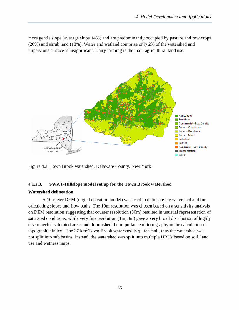
4. Model Development and Applications
35
more gentle slope (average slope 14%) and are predominantly occupied by pasture and row crops
(20%) and shrub land (18%). Water and wetland comprise only 2% of the watershed and
impervious surface is insignificant. Dairy farming is the main agricultural land use.
Figure 4.3. Town Brook watershed, Delaware County, New York
4.1.2.3. SWAT-Hillslope model set up for the Town Brook watershed
Watershed delineation
A 10-meter DEM (digital elevation model) was used to delineate the watershed and for
calculating slopes and flow paths. The 10m resolution was chosen based on a sensitivity analysis
on DEM resolution suggesting that courser resolution (30m) resulted in unusual representation of
saturated conditions, while very fine resolution (1m, 3m) gave a very broad distribution of highly
disconnected saturated areas and diminished the importance of topography in the calculation of
topographic index. The 37 km2 Town Brook watershed is quite small, thus the watershed was
not split into sub basins. Instead, the watershed was split into multiple HRUs based on soil, land
use and wetness maps.
Delaware County,
New York

2015 Water Quality Modeling Annual Report
36
HRU definition
Wetness map
A wetness map was created based on soil topographic index (STI) defined in Equation
(4.1). The upslope contributing area, α, was determined by the Terrain Analysis Using Digital
Elevation Models (TAUDEM) (Tarboton, 1997; Tarboton and Mohammed, 2010). The saturated
conductivity and soil depth were respectively extracted from two variables: saturated hydraulic
conductivity and depth to restricted layer in soil SSURGO database.
Based on the results from the Soil Moisture Routing (SMR) model of the Town Brook
watershed, Agnew et al. (2006) developed a relationship between STI and probability of
saturation (Psat
) for April, August and October representing spring, summer and fall conditions.
The study found that STI is a reliable parameter to identify and quantify the risk of saturation
excess runoff due to the clear, regionally consistent relationship between STI and Psat
with strong
correlation throughout the year. Based on the average results in the 3 seasonal conditions, Figure
4.4 shows that the areas with STI < 7.6 have almost no chance to be saturated; the areas with STI
> 17.7 are always saturated.
Figure 4.4. Relationship between topographic index (λ) and probability of saturation (Psat
) in April,
August and October (Agnew et al., 2006). The symbol are the average Psat
for corresponding λ.
The dashed lines correspond to 25th and 75th percentiles.
The Town Brook watershed was broken up into 5 wetness classes. Based on the results
from Agnew et al. (2006), we grouped the areas with STI < 7.6 as the “driest” wetness class
(wetness 5) with very high water storage capacity (1000mm) and the areas with STI > 17.7 as the
“wettest” wetness class (wetness 1) with no water storage capacity (0 mm). This means that
when there is hydrological input, the wetness 1 is always saturated while wetness 5 is constantly
dry. The rest of the watershed was classified into wetness class 2, 3 and 4 and their water storage
capacity were assigned by a trial method while running the model and comparing the results of

4. Model Development and Applications
37
saturated areas with our available observations in 28-30 April 2006 which is shown in Figure
4.10a. The final classification of 5 wetness classes in the Town Brook watershed is shown in
Figure 4.5. With this classification, only wetness 1, 2 and 3 can be saturated while wetness 4 and
5 are always dry. The maximum area of saturation is the summation of wetness 1, 2 and 3 which
equals to approximately 10% of the watershed. Harpold et al. (2010), from 6 field surveys in
2007, also reported 9.9% as the maximum saturated areas in a small study watershed in the
southwest corner of the Town Brook watershed.
Table 4.2. Classification of wetness classes for the Town Brook watershed.
STI Wetness % of watershed
area
Water storage
capacity Characteristics
< 7.6 5 5.1 1000 Dry
Wet
7.6 – 12.2 4 84.98 50
12.2 – 14.5 3 8.2 6
14.5 – 17.7 2 1.12 3
> 17.7 1 0.59 0
Figure 4.5. Wetness map for the Town Brook watershed

2015 Water Quality Modeling Annual Report
38
Soil
The soil map of Town Brook watershed was extracted from the SSURGO soil database.
There are 17 soil types in the watershed. The data of soil properties that are necessary for the
SWAT model are taken from the SSURGO database and the soil survey of Delaware County
(USDA, 2006). The soil map is then combined with the wetness map to redefine soil types in
different wetness classes in order to include wetness class assignment for each HRU in the final
discretization, which is an essential step for running SWAT-Hillslope.
Figure 4.6. Soil types in the Town Brook watershed (Source: SSURGO soil database)
Land use
The land use map was derived from classified 2009 aerial photography data obtained
from NYCDEP. The watershed was divided into 11 land use types which are shown in Figure 4.6
and Table 4.3. The main land use types are forest (54%), agriculture (32%) and brushland (9%).
Residential area covers a very small part of the watershed (4%).
Soil types_Town Brook
Bc
Bg
Bs
De
ElE
Ff
HcC
LhB
MaB
No
OeB
Rb
Re
TkB
VlB
W
WmB

4. Model Development and Applications
39
Table 4.3. Land use types in the Town Brook watershed
No. Land use type Percentage of area (%)
1 Forest - Coniferous 3.55
2 Forest - Deciduous 44.39
3 Forest - Mixed 5.83
4 Agriculture 32.10
5 Pasture 0.87
6 Brushland 8.94
7 Industrial 0.35
8 Commercial - Low density 0.02
9 Residential - Low density 3.73
10 Transportation 0.01
11 Water 0.21
Meteorological inputs
Daily precipitation and temperature data are available in a 4km x 4km gridded climate
dataset from the Applied Climate Information System (ACIS) which was developed using the
Parameter-Elevation Relationships on Independent Slopes Model (PRISM) interpolation method
(Daly et al., 2008). Thiessen polygons were created based on the available grid points to choose
the grid points that would be used for Town Brook watershed (Figure 4.7). As the Town Brook
watershed was setup as a single subbasin, precipitation and temperature data was assumed to be
taken at the centroid of the watershed by interpolating from data of surrounding PRISM grid
points by inverse distance weighting method.
Solar radiation was averaged from the data at the Albany and Binghamton airport
locations is available from 1926 to 2012. Relative humidity and wind speed were generated from
the weather generation method built in SWAT.

2015 Water Quality Modeling Annual Report
40
Figure 4.7. Meteorological grid points used for the Town Brook watershed
4.1.2.4. Model calibration and validation
Calibration was carried out at the outlet of the Town Brook watershed for the period
1998–2007 in which the first 3 years served as warming up period. The period of 2008–2012 was
the validation period. To evaluate the SWAT-Hillslope performance for the simulated flow, we
used three following criteria, each of which was calculated for daily and monthly time steps:
a. Nash Sutcliffe efficiency (NSE) (Nash and Sutcliffe, 1970): ranges between -∞ and 1.0, with
NSE = 1 being the optimal value.

4. Model Development and Applications
41
n
i
meanobs
i
n
i
sim
i
obs
i
YY
YY
NSE
1
2
1
2
)(
)(
1 (4.2)
where obs
iY is the ith observation, sim
iY is ith simulated value, sim
iY is the mean of observed data and
n is the total number of observations.
b. Percent bias (PBIAS): the optimal value of PBIAS is 0.0, with low magnitude values indicating
accurate model simulation. Positive values specify underestimation bias and negative values
indicate overestimation bias (Gupta et al., 1999).
n
i
obs
i
n
i
sim
i
obs
i
Y
YY
PBIAS
1
1
100*)(
(4.3)
c. RMSE – observations standard deviation ratio (RSR): RSR standardizes RMSE using the
observations standard deviation (Singh et al., 2004). It varies from the optimal value of 0, which
indicates zero RMSE to +∞. The lower RSR, the lower RMSE, the better the model performance.
2
1
1
2
)YY(
)YY(
STDEV
RMSERSR
meann
i
obs
i
n
i
sim
i
obs
i
obs
(4.4)
The SWAT-Hillslope model was calibrated by applying the Monte Carlo sampling
method. We randomly generated 10,000 parameter sets within the ranges of the chosen
parameters for calibration. Then 10,000 simulations were run with SWAT-Hillslope. Finally, the
best performance parameter sets were chosen. Table 4.4 shows the detailed parameters that were
used for calibration and their values that were used to evaluate SWAT-Hillslope performance by
comparing with observations. The calibration is performed in the following 3 steps, with steps 2
and 3 iterated:

2015 Water Quality Modeling Annual Report
42
1. Snow melt calibration: Five parameters related to snowmelt simulation were calibrated.
In the Town Brook watershed, snowmelt is a very important process. The snow melt
calibration helped to adjust the timing of flow peak when snow melt occurs.
2. Flow calibration: The best parameter set from the snowmelt calibration was used. Then
eleven flow parameter were taken into account in the Monte Carlo calibration (Table
4.4). The flow calibration affected the partition of flow components and flow magnitude.
3. Adjust storage capacity of wetness classes: The best parameter sets from snowmelt and
flow calibration were applied. Then the values of edc for wetness classes were calibrated
manually. This step influences the distribution of saturated areas caused by saturation
excess runoff.
4.1.3. Results
4.1.3.1. Performance of SWAT-Hillslope on flow simulation
The performance of SWAT-Hillslope on flow simulation was evaluated for simulation of
the hydrograph at the watershed outlet; flow components (runoff, lateral flow, baseflow); and the
spatial distribution of simulated runoff. The simulated results from the SWAT-Hillslope model
were compared with observations as well as the results from the original SWAT2012 model.
4.1.3.1.1. Comparison with measured hydrograph data at watershed outlet
The statistical evaluation of SWAT-Hillslope daily predictions versus measurements at
the outlet of Town Brook watershed (Table 4.5) resulted in NSE values at 0.68 and 0.52, PBIAS
values at 7.17 and -3.61, and RSR at 0.57 and 0.69 for calibration and validation periods,
respectively. These values are all within the range of “good” model performance for the
calibration period while NSE is rated as “satisfactory”, PBIAS as “very good” and RSR as
“satisfactory” performance in the validation period, based on Moriasi et al. (2007) guidelines for
evaluation of model performance. NSE improved significantly to 0.6 in the validation period if
we excluded the year 2011 in which an extreme flood occurred in August that could not be
captured very well by SWAT-Hillslope. The SWAT-Hillslope monthly predictions obtained
better fit to measurements with significantly improved NSE value at 0.87 and 0.78 for calibration
and validation periods, respectively. Monthly PBIAS values were comparable to daily ones while
monthly RSR values has improvement from daily values to be ranked as “very good”. Based on
statistical results on monthly streamflow, the performance of the SWAT-Hillslope model is
classified as “very good”, “good” and “very good” respectively corresponding to NSE, PBIAS
and RSR while it is classified as “very good” for all three indices in the validation period
whether the year 2011 was excluded or not.

4. Model Development and Applications
43
Table 4.4. Parameters for calibration using Monte Carlo sampling method
Name Unit Definition Range Calibrated
value
Snowmelt calibration
SFTMP oC Snowfall temperature -5 - 5 -0.58
SMTMP oC Snowmelt temperature -5 - 5 1.10
SMFMX mm/ oC Maximum snowmelt factor 5 - 10 7.62
SMFMN mm/ oC Minimum snowmelt factor 0 - 5 2.68
TIMP - Snow pack temperature lag factor 0 – 1 0.022
Flow calibration
RCHRG_PAF mm Fraction of root zone percolation
that recharges the perched aquifer
0-1000 0.626
latA Perched aquifer non-linear reservoir
coefficient
0 - 1 0.022
latB Perched aquifer non-linear reservoir
coefficient
1 - 3 1.72
ALPHA_BF - Baseflow alpha factor 0 - 1 0.23
GW_DELAY days Groundwater delay 0 - 200 28
EFFPORFACTOR mm Fraction of effective porosity that
can hold water under saturated
conditions
0 - 1 0.718
EDC_FACTOR - Calibration factor for adjusting edc
values
0.5 - 5 1.78
EPCO Plant water uptake compensation
factor
0 - 1 0.567
ESCO Soil evaporation compensation
factor
0 - 1 0.102
CANMX mm Maximum canopy storage 0 - 5 4.73
SURLAG days Surface runoff lag time 0.05 - 24 8.79
Storage capacity of wetness classes (5 wetness classes were defined in this case study
EDC01 mm Storage capacity of wetness class 1 0-1000 0
EDC02 mm Storage capacity of wetness class 2 0-1000 3
EDC03 mm Storage capacity of wetness class 3 0-1000 6
EDC04 mm Storage capacity of wetness class 4 0-1000 50
EDC05 mm Storage capacity of wetness class 5 0-1000 1000

2015 Water Quality Modeling Annual Report
44
Table 4.5. Performance criteria for SWAT-Hillslope in daily and monthly time step
Period Time
steps
Criteria
NSE PBIAS RSR Average streamflow (mm/a)
Simulated Observed
Calibration Daily 0.68 7.17 0.57 302.76 326.14
Monthly 0.87 7.25 0.36
Validation Daily 0.52 -3.61 0.69 331.61 320.05
Monthly 0.78 -3.38 0.46
Validation
(excluding 2011)
Daily 0.60 0.73 0.63 238.49 252.84
Monthly 0.82 1.03 0.43
The comparison between the SWAT-Hillslope and the original SWAT2012 models was
based on two calibrated models for Town Brook watershed. Figure 4.8 shows the comparison on
daily and monthly discharge values simulated by SWAT-Hillslope and SWAT2012 versus
observations for the period 2001-2003 which is within the calibration period. It is clearly
observed that SWAT-Hillslope was able to capture the variation of streamflow in both summer
(May – October) and winter (November to April) periods. However, SWAT-Hillslope
underestimated the flow in winter where snow melt occurred frequently and did not capture the
winter flow peaks excellently while it gave relatively comparable predictions of summer flows.
Compared to SWAT-Hillslope, although SWAT2012 was better in capturing the winter peaks, it
over-predicted the summer flows with simulated flow fluctuations in summers which had not
been observed during these periods. Moreover, it can be seen from month flow comparisons in
Figure 4.8 that SWAT2012 did not capture the flow trend as well as the SWAT-Hillslope model.
Figure 4.9 presents the scatter plots of the streamflow simulated by SWAT2012 and
SWAT-Hillslope versus measurements in daily and monthly time steps, relative to a 1:1 line plot.
It again shows the closer fit of both daily and monthly simulated streamflow from SWAT-
Hillslope to observed flow compared to SWAT2012. For daily time steps, SWAT-Hillslope
particularly showed better prediction for low flows. Generally, both models did not capture the
peak flows very well although SWAT2012 gave closer prediction to some extremely high flows.
Both models gave better performance for monthly predictions than daily ones. However, for all
the simulated months, SWAT-Hillslope gave closer fit to observations.

4. Model Development and Applications
45
Figure 4.8. Comparison of simulated daily and monthly discharge values between SWAT-
Hillslope, SWAT2012 and measured data

2015 Water Quality Modeling Annual Report
46
(a) Daily (b) Monthly
Figure 4.9. Scatter plot of daily and monthly simulated flow by SWAT-HS and SWAT2012 versus
observed flow
4.1.3.1.2. Comparison of simulated flow components
The estimated time series of three flow components: surface runoff, lateral flow and
groundwater flow by SWAT-Hillslope and SWAT2012 for the year 2003 are illustrated in Figure
4.10. Surface runoff was the dominant flow in SWAT2012 while lateral flow dominated in
SWAT-Hillslope. For the Town Brook watershed, SWAT-Hillslope predicted all surface runoff
coming from saturation excess process, the infiltration-excess runoff was estimated at 0, which is
reasonable for the Catskill Mountains area with infiltration rates often exceeding the medium
rainfall intensity. Lateral flow deriving from the perched aquifer in SWAT-Hillslope occurred
most of the time of the year except the period of snowfall (Jan – Feb). SWAT-Hillslope
estimated very stable groundwater flow which contributed to streamflow throughout the year, but
with small contribution at the beginning of the year when snowpack was accumulated. Different
from SWAT-Hillslope, surface runoff in SWAT2012 which is implicitly considered as
infiltration-excess runoff occurred in high rainfall except the snowfall period (Jan – Feb). Lateral
flow in SWAT2012 which derived from soil moisture excess from field capacity, occurred
throughout the year whenever there was rainfall. Groundwater flow had the same trend in the
two models with slightly more fluctuation in the SWAT2012 model because of high volume and
the difference in calibrated values for the groundwater-related parameters.
0
5
10
15
20
25
0 5 10 15 20 25
Sim
ula
ted
flo
w (
m3/s
)
Observed flow (m3/s)
SWAT2012
SWAT-Hillslope
0
1
2
3
4
0 1 2 3 4
Sim
ula
ted
flo
w (
m3/s
)
Observed flow (m3/s)
SWAT2012
SWAT-Hillslope

4. Model Development and Applications
47
(a) SWAT-Hillslope
(b) SWAT2012
Figure 4.10. Time series of flow components simulated by SWAT-Hillslope in comparison with
SWAT2012

2015 Water Quality Modeling Annual Report
48
(a) Wetness map (b) Land use
(c) Annual surface runoff in SWAT-Hillslope (d) Annual surface runoff in SWAT2012
Figure 4.11. Spatial distribution of annual surface runoff simulated by SWAT-Hillslope and
SWAT2012.
4.1.3.1.3. Comparison of Spatial Distribution of Runoff
The spatial distribution of annual surface runoff during the calibration period generated
by SWAT-Hillslope and SWAT2012 model was compared in Figure 4.11. Figure 4.11a and
Figure 4.11b depict the wetness and land use map of the Town Brook watershed while Figure
4.11c and Figure 4.11d present a striking difference in the spatial locations of surface runoff
production between SWAT-Hillslope and SWAT2012. The distribution of surface runoff
Wetness class

4. Model Development and Applications
49
predicted by SWAT2012 followed the distribution of land use in which forest contributed the
least runoff and agriculture was the most significant contribution. Residential areas had high
amount of surface runoff, however they covered very small area in the watershed. Surface runoff
was generated all over the watershed in SWAT2012 because it closely depended on land use due
to the concept of Curve number. Unlike SWAT2012, runoff predicted by SWAT-Hillslope was
only found in the areas corresponding to wetness class 1, 2 and 3 which were considered to be
prone to saturation and were set with low water storage capacity.
Moreover, the spatial distribution of simulated saturated areas by SWAT-Hillslope was
compared with available observations in 28-30/4/2006 in a small area in Town Brook watershed
(Figure 4.12). Figure 4.12a and Figure 4.12b respectively show the observed and simulated
saturated areas by SWAT-Hillslope in the three observed days while Figure 4.12b presents the
variation of rainfall in April, 2006. From Figure 4.12c, no rainfall was observed from 28-
30/4/2006 while there was a big storm happening on 23/04/2006. Due to no rainfall event,
SWAT2012 predicted no surface runoff from 28-30/04/2006. In contrast, SWAT-Hillslope
predicted the presence of saturation areas in these three days which is compatible with the
observations. The saturation was caused by the high water level in perched aquifer resulting from
the big storm event on 23/04/2006 and lateral flow contribution from the upslope areas to the
downslope areas which are prone to saturation.
4.1.4. Discussion
Correctly identifying surface runoff source areas is particularly important for SWAT
model applications to support watershed management. An effective watershed management
strategy for pollution control is to target areas on the landscape where surface runoff and
transportable pollutants co-occur (Gburek et al., 2002; Walter et al., 2000; Zollweg et al., 1996).
Two runoff generation mechanisms - infiltration excess runoff and saturation excess runoff - can
produce very different spatial distributions of runoff (Easton et al., 2008; Schneiderman et al.,
2007). Infiltration excess runoff occurs where rainfall rates exceed infiltration capacity of the
soil, while saturation-excess runoff occurs on variable source areas (VSAs) that saturate from
below. Overland flow is generated at VSAs by a combination of rainfall and return flow (lateral
flow in SWAT terminology), and return flow may be the dominant source of stormflow in
catchments where VSAs occur but are limited in extent (Walter et al., 2000). Different areas in
the same catchment may exhibit infiltration excess runoff, saturation excess runoff, and return
flow in various combinations. It is thus important in watershed pollutant export modeling
applications to explicitly account for these hydrological processes.
SWAT-Hillslope improves upon SWAT's ability to identify runoff source areas and
hydrologic flow paths by replacing the runoff curve number method with explicit calculation of
infiltration excess runoff, saturation excess runoff, and return flow at saturated areas. The curve
number equation represents an empirical relationship between rainfall and runoff on a watershed

2015 Water Quality Modeling Annual Report
50
scale but does not account for the underlying processes of runoff generation. SWAT-Hillslope
proceeds in the following order for each HRU: i) estimate infiltration-excess runoff and
infiltration using Green-Ampt method (Green and Ampt, 1911; Mein and Larson, 1973; Neitsch
et al., 2011), ii) determine saturation-excess runoff and saturated areas using a statistical-
dynamical approach to simulating the perched aquifer, and 3) estimate return flow at saturated
areas as a non-linear function of perched aquifer storage.
Figure 4.12. Saturated areas simulated by SWAT-Hillslope compared with observations.
The statistical-dynamical (SD) approach to simulating the behavior of a perched aquifer
(Wigmosta and Lettenmaier, 1999) treats the mean height of a perched water table as a time-
varying dynamic process while the shape of the water table (i.e., the spatial distribution of depth
(a) Observations of saturated areas in
28-30/04/2006
(b) Saturated areas by SWAT-Hillslope
(c) Rainfall in April 2006

4. Model Development and Applications
51
to water table) within the hillslope is based on a statistical distribution of soil water storage
capacity. The water table as a whole moves up and down as the average depth of water in the
perched aquifer changes, while the shape of the water table remains constant over time (Figure
4.13). A number of models utilize this approach, including TOPMODEL (Beven and Kirkby,
1979; Sivapalan et al., 1997), the Variable Infiltration Capacity (VIC) model (Liang and
Lettenmaier, 1994; Wood et al., 1992), the Probability Distributed Model (PDM) (Moore, 2007),
the XINANJIANG model (Zhao et al., 1995), and the Australian Water Balance Model (AWBM)
(Boughton, 2004). The efficiency of this approach has been studied most for TOPMODEL. The
topographic wetness index (TWI) which defines the soil water storage capacity distribution in
TOPMODEL has been shown to be fairly well correlated with observed soil moisture patterns in
a number of studies including for the Town Brook watershed (Agnew et al., 2006; Buchanan et
al., 2014; Grabs et al., 2009; Harpold et al., 2010; Lyon et al., 2004; Moore and Thompson,
1996; Troch et al., 1993), but others have found that the TWI may not fully describe the
observed soil moisture patterns and that other factors not captured by the index may significantly
influence wetness distributions (Buttle et al., 2001; Güntner et al., 2004; Hjerdt et al., 2004;
Iorgulescu and Jordan, 1994; Seibert et al., 2003).
Figure 4.13 Idealized hillslope profile according to statistical dynamic approach. Water table
saturates at location 1, intersects the root zone at location 2, and is below the root zone at
location 3.
SWAT-Hillslope adopts the variable bucket approach of Sivapalan et al. (1997) and
Boughton (2004) and others for defining the distribution of soil water storage capacity. A user-
defined distribution is input by dividing the catchment into a set of subareas of increasing storage
capacity and specifying the area and maximum storage capacity of each areal wetness class. The
moisture distribution may be parametric, as in TOPMODEL, VIC, PDM and XINANJIANG
models; or empirically derived as in AWBM model. In the application of SWAT-Hillslope in the
2015 Water Quality Modeling Annual Report
52
Town Brook watershed, the latter approach was taken. A previous analysis of observed soil
moisture distribution in relation to the TWI was used to define 5 wetness classes and associated
maximum soil moisture storage capacity distribution (Table 4.2). The resultant model performed
well in simulating VSAs with a maximum extent of ~10% in accordance with observations as
well as the hydrograph at the basin outlet, with hydrograph peaks being composed of substantial
return flow.
For catchments where soil moisture data is not available to inform the storage capacity
distribution, it may be useful to consider defining catchment wetness classes at least initially
according to a basic wetness classification scheme (from wet to dry), for example: 1) perennial
stream channel; 2) perennial wetlands; 3) seasonally-saturated wetlands; 4) intermittently
saturated areas; 5) rarely or never saturated. A basic wetness classification may be parametrized
using a variety of information, including soil survey hydrologic data, wetland maps,
farmer/landowner observation knowledgebase. It may also be useful to consider the shape of a
storage capacity distribution developed from soft data as falling between two extreme cases
(Figure 4.14): (a) a catchment with limited benches and floodplains, limited maximum extent of
VSAs, and characterized by a TWI storage capacity distribution, vs. (b) one with extensive
floodplains, extensive extent of VSAs, and characterized by a pareto distribution with b>1
(Moore 2007). Alternatively, the moisture capacity distribution can be derived directly from the
TWI distribution as in the variable bucket representation of TOPMODEL of Sivapalan (1997).
The TWI distribution is transformed to a storage capacity distribution (S) by:
)(*_ max TWITWIfactoredcS (4.5)
where TWImax is the maximum TWI value for the catchment, and edc_factor serves as the
TOPMODEL’s 1/f hydrogeological parameter, a measure of the assumed exponential decrease of
soil hydrologic conductivity with depth. Use of distribution (x) effectively equates the saturation-
excess runoff algorithm in SWAT-Hillslope with a TOPMODEL application.

4. Model Development and Applications
53
Figure 4.14. Water capacity distribution functions for two different topographic regimes. a) with
limited benches and floodplains, limited maximum extent of VSAs, and characterized by a TWI
storage capacity distribution. b) catchment with extensive floodplains, extensive extent of VSAs,
and characterized by a pareto distribution with b>1 (Moore 2007).
4.1.5. Conclusions
When applied to the Town Brook watershed, the modified version of SWAT, SWAT-
Hillslope, successfully separates the infiltration excess runoff and saturation excess runoff.
SWAT-Hillslope performed well in flow simulation for both daily and monthly time steps.
Moreover, the comparison on spatial distribution of saturated areas with available observation in
the three days with no precipitation showed that SWAT-Hillslope model was able to correctly
predict the locations of saturated areas while the original SWAT could not predict any surface
runoff in these dry days. SWAT-Hillslope allows the transportation of interflow laterally from
upslope to downslope areas, providing water to saturate the wet HRUs. In addition, the perched
aquifer has close interaction with the soil profile, which keeps the water level stay high in wet
HRUs. Based on the good performance of SWAT-Hillslope both on streamflow simulation and
spatial runoff distribution, it can be confidently concluded that with the incorporation of
topography characteristics and the adding of the perched aquifer, SWAT-Hillslope gives a
realistic representation of hydrological processes and is expected to lead to better water quality
models where the source of the surface runoff matters.
b) a)

2015 Water Quality Modeling Annual Report
54
4.2. Application of the General Lake Model (GLM) to Cannonsville and
Neversink Reservoirs
A major new modeling initiative at DEP involves disinfection byproducts (DBPs) in the
water supply. DBPs are formed when chlorine is added to water as a disinfectant in order to
inactivate bacteria, viruses, and other pathogens. A portion of the naturally-occurring organic
compounds found in tributary streams and water supply reservoirs reacts with chlorine to form
DBPs; this group of compounds which form DBPs are collectively known as the DBP precursors
(DBPP). DEP seeks to better understand the role of both external watershed loading and internal
reservoir production of dissolved organic carbon (DOC) and DBPPs, and the effect of watershed,
terrestrial, and reservoir processes which act as sources and sinks for these chemicals. The role
of climate change on levels of DOC and DBPPs in the water supply is also of significant interest.
A goal of this work is to develop a predictive model for DOC and DBPP that may be used in
guiding watershed protection activities, evaluating impacts of climate change, and integrated into
DEP’s Operations Support Tool (OST) to guide operations to minimize DBPPs in the water
supply and DBPs in the distribution system.
The General Lake Model (GLM), linked with the Aquatic Ecodynamics model (AED),
has been selected for application and testing in predicting DOC and DBPPs in DEP reservoirs.
GLM/AED is an open source community lake and reservoir model that has been developed as an
initiative of the University of Western Australia and the Global Lake Ecological Observatory
Network (GLEON), and has been applied to numerous lakes and reservoir within the GLEON
network and beyond. In its current form, GLM/AED is capable of simulating the organic carbon
cycle, but is not capable of predicting DBPP. Working with postdoctoral researchers and
associated university faculty advisors, DEP modeling staff will be developing enhancements to
this model to allow prediction of DBPP. Cannonsville and Neversink Reservoirs have been
selected for initial development and testing of this model.
Here the application and testing of the hydrothermal component of GLM to Cannonsville
and Neversink is described. Hydrothermal testing and validation is a critical first step in the
process of model application and testing, as the predictions of water temperature and internal
reservoir mixing and transport that are a part of the hydrothermal predictions affect the
subsequent predictions of all water quality parameters.

4. Model Development and Applications
55
4.2.1. Methods
4.2.1.1. Study sites
Cannonsville and Neversink Reservoirs, two NYC reservoirs with different catchment
characteristics, were chosen to test if GLM is capable of simulating in NYC reservoirs (Figure
4.15). The Neversink Reservoir watershed is 91% forested with very little agriculture (1.4%) and
developed land (3%). In contrast, land use in the Cannonsville Reservoir watershed is about 19%
agricultural with an additional 7% categorized as developed. The GLM model was applied to
these two reservoirs for the historical conditions that occurred in 2007 and 2008.
(a) Cannonsville (b) Neversink
Figure 4.15. Land use within the watersheds of (a) Cannonsville Reservoir, and (b) Neversink
Reservoir.
4.2.1.2. GLM Model set up
Bathymetric curves relating reservoir surface area and storage volume to water surface
elevation are required for operation of GLM. The bathymetric curves for Cannonsville (Figure
4.16) and Neversink Reservoirs (Figure 4.17) contained in The New York City Water Supply
Atlas were used in GLM simulations. In addition, the elevation of the spillway, and elevations of
drinking water intakes as used in the GLM model are given in Table 4.6.

2015 Water Quality Modeling Annual Report
56
Figure 4.16. Bathymetric curves for Cannonsville Reservoir.
Figure 4.17. Bathymetric curves for Neversink Reservoir.

4. Model Development and Applications
57
4.2.1.3. Meteorological inputs
The GLM model requires daily values of various meteorological data, including solar
radiation, air temperature, relative humidity, wind speed, rain and snow. Daily values of these
quantities for 2007 and 2008 taken from DEP records, are shown in Figure 4.18 for Cannonsville
Reservoir, and Figure 4.19 for Neversink Reservoir.
4.2.1.4. Water budget calculation
A water budget calculation was performed independently and prior to GLM simulations.
The goal of the water budget calculation was to determine daily values of the ungaged inflow to
a reservoir, so that, when used as a model input for a historical period, the predicted reservoir
water surface elevation closely matches the observed elevation. The water balance or budget
equation used was:
OIUIG QQQdt
dV (4.6)
where V is reservoir volume, t is time, QIG is the gaged surface inflow, QIU is the ungaged
surface inflow, and QO is the total outflow. This is the same water budget equation described in
Section 5.1 of this report. For Cannonsville Reservoir, USGS streamflow records for the West
Branch of the Delaware River at Beerston, and for Trout Creek at Trout Creek, represented the
gaged inflows. For Neversink, USGS observations of the Neversink River at Claryville was the
single gaged inflow to the reservoir. For both reservoirs, the outflow QO is the sum of drinking
water withdrawal, dam release, and spill. Using these observations and Equation (4.6), daily
values of the ungaged inflow QIU were determined as described in Section 5.1. The reservoir
inflows and outflows for Cannonsville Reservoir for 2007-2008 are shown in Figure 4.20, while
the inflows and outflow for the same years for Neversink Reservoir are shown in Figure 4.21.

2015 Water Quality Modeling Annual Report
58
Table 4.6. Spillway and Intake Elevations of Cannonsville Reservoir and Neversink Reservoir.
Site Elevation
(ft) (m)
Cannonsville
Cannonsville Reservoir Spillway Elevation 1150.00 350.52
Cannonsville Reservoir Elevation Tap 1 (CR1) 1032.00 314.55
Cannonsville Reservoir Elevation Tap 2 (CR2) 1077.75 328.50
Cannonsville Reservoir Elevation Tap 3 (CR3) 1113.65 339.44
Neversink
Neversink Reservoir Spillway Elevation 1440.00 438.91
Neversink Reservoir Elevation Tap 1 (NR1) 1314.00 400.51
Neversink Reservoir Elevation Tap 2 (NR2) 1344.00 409.65
Neversink Reservoir Elevation Tap 3 (NR3) 1374.00 418.80
Neversink Reservoir Elevation Tap 4 (NR4) 1404.00 427.94
Note: elevations use Bureau of Water Supply (BWS) datum

4. Model Development and Applications
59

2015 Water Quality Modeling Annual Report
60
Figure 4.18. Meteorological data for Cannonsville Reservoir, 2007-08.

4. Model Development and Applications
61

2015 Water Quality Modeling Annual Report
62
Figure 4.19. Meteorological data for Neversink Reservoir, 2007-08.

4. Model Development and Applications
63
Figure 4.20. Components of the water budget for Cannonsville Reservoir, 2007-2008: (a)
inflows, and (b) outflows.

2015 Water Quality Modeling Annual Report
64
Figure 4.21. Components of the water budget for Neversink Reservoir 2007-2008: (a)
inflows, and (b) outflows.
4.2.1.5. Tributary Stream Temperature
The temperature of tributary streams is a required input for GLM. Using DEP records,
the temperature of stream inflows to for Cannonsville and Neversink Reservoirs in 2007 and
2008 are shown in Figure 4.22.

4. Model Development and Applications
65
Figure 4.22. Inflow temperatures of Cannonsville Reservoir (a) and Neversink Reservoir (b).
4.2.1.6. Model calibration and validation
The primary goal in this application of the GLM hydrothermal model is the accurate
simulation of the temperature of the entire water column, including the surface temperature (0-
3m) and the bottom water layer (at variable depth) for the entire whole simulation period. Model
simulations began on first date of water column temperature measurements in each of two years,
for each reservoir, and continued to the end of year (Table 4.7). The predicted water column
temperatures were compared to routine DEP temperature observations. The whole water column
was first manually calibrated and then an auto calibration procedure was applied to reduce root
mean square errors (RMSE) in the predicted water column temperature. The key hydrothermal
model parameters coefficients that were adjusted as a part of the calibration process are given in
Table 4.8.
Table 4.7. The simulation period for Cannonsville Reservoir and Neversink Reservoir.
Cannonsville Neversink
Calibration Start 4 April 2007 24 April 2007
End 31 December 2007 31 December 2007
Validation Start 4 April 2008 14 April 2008
End 31 December 2008 31 December 2008

2015 Water Quality Modeling Annual Report
66
Table 4.8. GLM hydrothermal model coefficients that were adjusted during model calibration.
Symbol Parameter Description Default Cannonsville Neversink
hmin Minimum layer thickness (m) 0.5 0.25 0.25
hmax Maximum layer thickness (m) 1.5 0.5 0.5
CK Mixing efficiency – convective
overturn
0.2 0.125 0.125
CW Mixing efficiency – wind stirring 0.23 0.1033 0.1033
CS Mixing efficiency – shear
production
0.3 0.0407 0.4868
CT Mixing efficiency – unsteady
turbulence
0.5 0.51 0.51
CKH Mixing efficiency – Kelvin-
Helmholtz turbulent billows
0.3 0.285 0.285
CHYP Mixing efficiency – hypolimnetic
turbulence
0.5 0.52 0.47
KW Extinction coefficient for PAR
Radiation (m−1)
0.2 0.7396 0.5023
AC Critical area below which wind
sheltering may occur (m2)
107 107 107
Wind factor Wind multiplication factor 1.0 1.2676 1.0648
CE Bulk aerodynamic coefficient for
latent heat transfer
0.0013 0.0014 0.0022
CM Bulk aerodynamic coefficient for
transfer of momentum
0.0013 0.0013 0.0013
CH Bulk aerodynamic coefficient for
sensible heat transfer
0.0013 0.0013 0.0013
𝜆 Latent heat of evaporation (J/Kg) 2.453×10⁶ 2.453×10⁶ 2.453×10⁶
𝜎 Stefan-Boltzmann constant
(W/m2/K4)
5.67×10⁻⁸ 5.67×10⁻⁸ 5.67×10⁻⁸
𝜀a Emissivity of the water surface 0.985 0.985 0.985
CD Streambed drag 0.016 0.016 0.016
G Seepage rate (m/d) 0 0 0

4. Model Development and Applications
67
4.2.2. Results and Discussion
4.2.2.1. Water balance
The GLM simulated water surface elevation for Cannonsville Reservoir is shown in
Figure 4.23. The good agreement between predictions and observations reflects the accurate
calculation of ungaged inflows, and the accuracy of the bathymetric curves. The results for
Neversink Reservoir (Figure 4.24) as similarly good. During the calibration and validation
period, the simulated water surface elevation was generally highest in the spring and lowest in
the fall both in Cannonsville Reservoir and Neversink Reservoir, which reflected the observed
water surface elevation.
Figure 4.23. Simulated water level (grey) and observed water level (black) of Cannonsville
Reservoir (dash line is the spillway elevation).

2015 Water Quality Modeling Annual Report
68
Figure 4.24. Simulated water level (grey) and observed water level (black) of Neversink
Reservoir (dash line is the spillway elevation).
4.2.2.2. Temperature simulation
Calibration on the hydrothermal component of GLM was based comparison on predicted
and observed temperatures for 2007 only. Once the calibration step was completed, the
calibrated model was then applied to each reservoir for 2008, in order to separately validate the
calibrated model.
The thermal structure of Cannonsville and Neversink Reservoirs as simulated by GLM is
shown in Figure 4.25 and Figure 4.26, respectively. Comparison of predicted and observed
temperatures in the surface and the bottom water layers of Cannonsville and Neversink
Reservoirs are shown in Figure 4.27 and Figure 4.28, respectively. The seasonal variation in the
temperatures of both water layers was captured well. The RMSE values for simulated
temperatures over the entire water column for each reservoir for 2007 (calibration) and 2008
(validation) are summarized in Table 4.9. As expected, the temperature errors were modestly
larger for the validation period (2008) relative to the calibration period (2007). Moreover, the
accurate prediction of bottom water temperature is an indication that vertical mixing between the
surface and bottom waters is simulated accurately.
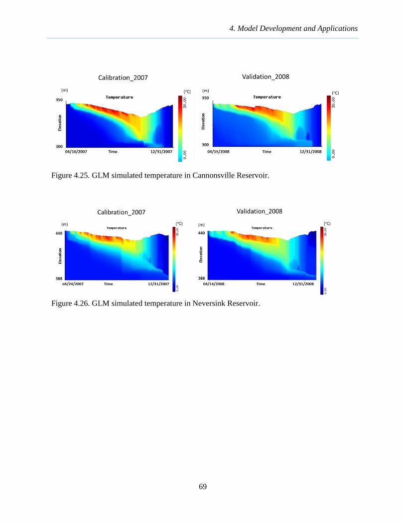
4. Model Development and Applications
69
Figure 4.25. GLM simulated temperature in Cannonsville Reservoir.
Figure 4.26. GLM simulated temperature in Neversink Reservoir.

2015 Water Quality Modeling Annual Report
70
Figure 4.27. GLM simulated temperature for the surface water layer (a) and the bottom water
layer (b) in Cannonsville Reservoir.
Figure 4.28. GLM simulated temperature for the surface water layer (a) and the bottom water
layer (b) in Neversink Reservoir.

4. Model Development and Applications
71
Table 4.9. The average root mean square error (RMSE) in predicted water column
temperatures (oC).
Cannonsville Neversink
Calibration_2007 1.77 1.84
Validation_2008 1.95 2.56
For Cannonsville Reservoir, observed water column temperatures at site 4 were used for
model calibration and validation. The one dimensional (1D) GLM model has a good model
performance for predicting water column temperatures with the observed data at all sites in NYC
reservoirs. During the calibration period (2007), the GLM simulated temperature profiles not
only matched the field data at Site 4 well in Cannonsville Reservoir (Figure 4.29) but also
matched well the observed data at all sites of Cannonsville Reservoir (Figure 4.30). During the
validation period of 2008, the predicted temperature profiles matched the observed temperature
profiles at all sites of Cannonsville Reservoir (Figure 4.31). GLM model predictions for
Neversink for the calibration year (2007) are shown in Figure 4.32 and Figure 4.33, and
validation results depicted in Figure 4.34. For Neversink Reservoir, observations for Site 1 were
the basis for model calibration and validation. The observed temperature profiles in
Cannonsville (Figure 4.30 and Figure 4.31) and Neversink (Figure 4.33 and Figure 4.34) indicate
that there is little horizontal variation in water temperature from site to site. This indicates that, at
least with respect to simulation of temperature, the one dimensional assumption is valid. The
features of thermal stratification in both reservoirs were reproduced well in summer. This
modeling feature is very important for simulating algal blooms and other water quality features.
In the epilimnion, the interannual variation (2007 relative to 2008) of temperature was simulated
well, which indicates that the GLM model has the ability of predicting the surface heat transfer
and wind mixing. However, in the metalimnion and hypolimnion, the simulated temperatures on
some specific dates were modestly lower than observations. Although some simulated
thermocline depths did not always match the observed depths accurately, the simulated
thermocline depth increased from summer to fall, which matched the observed pattern. These
results are generally similar to that obtained the previous application of a one dimensional
hydrothermal model to Cannonsville (Owens, 1998). Overall, the GLM model succeeded in
tracking the seasonal changes of temperature in these two reservoirs.

2015 Water Quality Modeling Annual Report
72
Figure 4.29. Simulated temperature profiles and field data at Site 4 in Cannonsville Reservoir
in 2007.
Figure 4.30. Simulated temperature profiles and field data at all sites of Cannonsville
Reservoir in 2007.

4. Model Development and Applications
73
Figure 4.31. Simulated temperature profiles and field data at all sites of Cannonsville
Reservoir in 2008.

2015 Water Quality Modeling Annual Report
74
Figure 4.32. Simulated temperature profiles and field data at Site 1 in Neversink Reservoir
in 2007.
Figure 4.33. Simulated temperature profiles and field data at all sites of Neversink Reservoir
in 2007.

4. Model Development and Applications
75
Figure 4.34. Simulated temperature profiles and field data at all sites of Neversink for 2008.
DEP observations of the temperature of the drinking water withdrawal were also
compared with model predictions. This comparison not only tests the ability of the model to
simulate water column temperature, but also tests the simulation of selective withdrawal

2015 Water Quality Modeling Annual Report
76
algorithms in the model. Although there was under prediction of withdrawal temperatures in the
spring and early summer, the simulated trend of withdrawal temperatures was generally
consistent with the observation in Cannonsville Reservoir (Figure 4.35). The blank area in the
withdrawal temperature in Figure 4.35 indicates that there was no withdrawal. There was a
consistently large difference between simulated and observed withdrawal temperatures in
Neversink Reservoir (Figure 4.36). Additional calibration of selective withdrawal model
coefficients (Hipsey et al., 2014) will be pursued for Neversink Reservoir in the future.
(a) (b)
Figure 4.35. Simulated withdrawal temperatures (lines) and observed withdrawal
temperatures (circles) of Cannonsville Reservoir: (a) 2007, and (b) 2008.
(a) (b)
Figure 4.36. Simulated withdrawal temperatures (lines) and observed withdrawal
temperatures (circles) of Neversink Reservoir: (a) 2007, and (b) 2008..

4. Model Development and Applications
77
4.3. Development and Testing of a Probabilistic Turbidity Model for
Rondout Reservoir
4.3.1. Background
NYCDEP now routinely uses the Operations Support Tool (OST) software (Hazen and
Sawyer 2013) to help guide reservoir operating decisions involving both the quantity and quality
of water. An important water quality parameter of concern for the City’s water supply is
turbidity. To address this, OST employs a two-dimensional (longitudinal-vertical) multiple size-
class turbidity model (Gelda and Effler 2007, Gelda et al. 2009, 2012, 2013) based on the mass
transport framework of CE-QUAL-W2 (W2; Cole and Wells 2013). For managing water
quantity, OST includes the entire Delaware River Basin, the Catskill subsystem, and the Croton
subsystem, though water quality (turbidity) models that have been integrated into OST are for
Schoharie, Ashokan, and Kensico reservoirs only.
In the current version of OST, models for Schoharie and Ashokan reservoirs provide
input of turbidity from the Catskill Basin to the Kensico Reservoir model, while input of
turbidity from the Delaware Basin (mostly Rondout Reservoir water) is specified at historical
median values. Here we develop a tool to forecast more realistic simulations of turbidity in
Rondout Reservoir withdrawal which can then be specified as input to Kensico Reservoir
turbidity model in OST thus making the forecasts of turbidity in the Kensico Reservoir
withdrawal more accurate.
The proposed modeling tool is based on a separate turbidity model for Rondout
Reservoir, which was developed and validated earlier (Gelda et al. 2013). With the added
capability of using short-term ensemble forecasts of hydrological inputs, turbidity, and
climatology as the model drivers, it can generate probabilistic forecasts of turbidity. The tool is
expected to help guide operations of Rondout Reservoir during storm events in the watershed as
well as provide realistic estimates of turbidity inputs for the Kensico Reservoir model in OST.
4.3.2. Approach
The central feature of the overall probabilistic modeling framework is the deterministic
hydrodynamic-water quality model, W2 (Figure 4.37). It is capable of simulating transport
within the reservoir, features of the thermal stratification regime, temperature in the withdrawal,
patterns of turbidity within the reservoir, and in the withdrawal. The model drivers are
meteorological conditions, inflows, inflow-temperatures, and inflow-turbidity from Rondout
Creek, Chestnut Creek, and Cannonsville, Pepacton, and Neversink tunnels (Figure 4.38).

2015 Water Quality Modeling Annual Report
78
With the best forecasts of the model drivers, W2 can generate a single best forecast of
turbidity. However, such forecast has limited management value because there is no probability
associated with it. Further, the forecasts of model drivers have natural variability and uncertainty,
which is not represented in the model if only best estimates are used. The probability approach
presented here incorporates variability and uncertainty in the model inputs, including
meteorological, hydrological, and water quality data (Figure 4.37). The model output generated
from this approach is analyzed in a probabilistic format, allowing managers to make risk-based
operations decisions. The details of this approach are discussed next.
Figure 4.37. Conceptual framework of a probabilistic turbidity model for Rondout Reservoir.
(NOAA: National Oceanic and Atmospheric Administration, HEFS:
Hydrologic Ensemble Forecast System, OST: Operations Support Tool)
Definitions: Multiple time series of forecast are known collectively as an ensemble of
forecast and an individual time series in an ensemble is referred to as an ensemble member. The
values in a time series (or an ensemble member) when used in a model as an input can be called
a trace. Linked input traces of meteorology, hydrology, and water quality together with the
corresponding model output trace will form a complete model simulation trace. Such multiple
simulation traces form the basis of ensemble reservoir water quality forecasts which are then
used to construct probabilistic predictions.

4. Model Development and Applications
79
Figure 4.38. CE-QUAL-W2 model segmentation of Rondout Reservoir, including monitoring
location on the tributaries, and in the reservoir. Inputs from the upstream
Cannonsville, Pepacton, and Neversink reservoirs are indicated by WBDT,
EDT, and NST, respectively.
Method: Ensemble forecasts of atmospheric conditions (e.g., temperature, precipitation)
by National Oceanic and Atmospheric Administration (NOAA) are used by National Weather
Service’s (NWS) hydrologic models to generate hydrologic ensemble forecasts. These forecasts
are accessed and post-processed by OST. The post-processing step corrects any statistical bias in
the forecasts, formats data according to the input requirements of OST, and develops flow inputs
for the locations in the model (Figure 4.37).
The modeling tool developed here, obtains from OST, traces (n = 47) of total inflow to
Rondout Reservoir and divides into inflow from Rondout Creek, Chestnut Creek, and ungaged
area (Figure 4.38), as required by W2 model. Corresponding to each of these hydrologic traces, a
time series trace of turbidity is estimated from the empirical relationships developed between
flow and turbidity (UFI 2013).
Site-specific short-term (e.g., days–weeks) forecasts of hourly meteorological data (air
temperature, dew point temperature, wind speed and direction, and solar radiation)
corresponding to the hydrologic traces are not available presently. Therefore, historical data
available for the 1987-2012 (m = 25) interval were used. To combine the variability present in
the hydrological data with the variability present in the meteorological data, m W2 model runs
were made for each hydrological and water quality trace input, for a total of m × n (25 × 47 =

2015 Water Quality Modeling Annual Report
80
1125) runs (Figure 4.37). Additional inputs required by W2 model are initial state (i.e.,
temperature, water surface elevation and turbidity) of the reservoir and reservoir operations
(inflows from the three upstream reservoirs, and withdrawal). The following section describes an
example application of the approach and compares the predicted turbidities in the withdrawal, in
a probabilistic context, with the actual observations.
4.3.3. Model Specifications for an Example Application
The model was applied to forecast turbidity in the withdrawal from Rondout Reservoir
during a period of 11/13/2015–12/1/2015 (18 days). All hydrodynamic and water quality model
parameters were adopted from the previously validated model (Gelda et al. 2013).
Future boundary conditions: Hydrologic ensemble forecast included 47 traces of total
inflow, which was processed into three separate inflows from Rondout Creek, Chestnut Creek,
and ungaged area represented in the model as distributed along the shoreline, according to the
respective watershed areas. Turbidity associated with each hydrologic trace and source input was
estimated according to the empirical relationships developed by UFI (2013). The contribution to
the total turbidity from the three size classes of particles was estimated as specified by UFI
(2013). Meteorology was obtained from the historical database developed for the reservoir site
for 1987–2012 (25 year-long individual traces). Inflow temperatures were also obtained from the
historical observations for the same interval. A trace of inflow temperature corresponded to the
same time trace of meteorology.
Reservoir Operations: Inputs from the three upstream reservoirs – Cannonsville,
Pepacton, and Neversink reservoirs – were specified as listed in Table 4.10. Neversink Tunnel
was not in operations during the study period. Withdrawal and downstream release from
Rondout Reservoir were set at 700 MGD, and 10 MGD, respectively. The elevation of the intake
in use was 784 feet.
Initial conditions: The observed water surface elevation at the beginning of the forecast
period was 836 feet. Initial values of the temperature and turbidity in the reservoir were obtained
by linearly interpolating observations, from 3 sites and 3–4 depths at each site, made during a
routine field survey on 11/10/2015 (Table 4.11).

4. Model Development and Applications
81
Table 4.10. Specifications of operations of upstream reservoirs for the forecast
interval of 11/13/2015–12/1/2015.
Source Flow+ Temperature* Turbidity*
Pepacton 500 MGD historical median daily;
daily values
historical 10th percentile
daily; daily values
Cannonsville 200 MGD historical median daily;
daily values
historical median daily;
daily values
Neversink 0 - - +option for choosing any time series will be added; specified flows were approximately equal to
the actual operations and were projected to continue for the forecast period. *option for choosing historical 5th, 10th, 25th, 75th, 90th, 95th percentile values or any time
series is available.
Table 4.11. Observed temperature and turbidity depth
profiles at sites 1, 2, and 3 in Rondout
Reservoir on 11/10/2015.
Site Depth
(m)
Temperature
(°C)
Turbidity
(NTU)
1 3 12.7 0.8
1 20 12.1 0.85
1 36 8.8 0.85
1 47 7.5 1.6
2 3 12.5 0.7
2 17 12.4 0.6
2 32 11.3 1.5
3 3 12.3 0.9
3 14 12.3 0.6
3 25 11.1 1.4
4.3.4. Results and Discussion
Substantial variability was forecasted in the Rondout Creek inflow for the study period
by Hydrologic Ensemble Forecast Service (HEFS) as depicted in Figure 4.39 by the 47
individual traces of inflow time series. The variability in the flow existed both from day to day
and amongst the traces, however, the median forecast was nearly steady at about 1.25 m3 s−1 for

2015 Water Quality Modeling Annual Report
82
the duration of the study. Observations, which became available after the study, generally
tracked the 90th percentile of the ensemble (Figure 4.39).
The full combined variability in the model output arising from the variability in the
model drivers (hydrology, meteorology, and water quality, i.e., turbidity) is evaluated here for
the predictions of turbidity in the withdrawal, a key point of water quality concern (Figure 4.40).
Out of 1175 individual traces (47 hydrology traces × 25 meteorology traces) of predictions, only
100 are shown in Figure 4.40, however, the median, 10th and 90th percentiles depicted are
obtained from all 1175 traces.
Figure 4.39. Ensemble forecast of Rondout Creek inflow for 11/13/2015–12/1/2015. Forty
seven individual traces, median, 10th and 90th percentile traces are shown along with the
observations from USGS.
The median forecast of turbidity indicated a modest downward trend during the study
period, from ~ 0.85 NTU on 11/13/2015 to ~ 0.65 NTU at the end of the period on 12/1/2015
(Figure 4.40). Some of the individual traces predicted turbidity > 1.5 NTU after 11/26/2015 due
to a couple of inflow traces that included a forecast of high runoff, and correspondingly high
turbidity, on that day. Two such inflow traces combined with 25 meteorological traces resulted in
50 traces of anomalous withdrawal turbidity, which did not affect the median forecast (Figure
4.40).
The observations of turbidity for the same time interval provided the opportunity to
validate the model forecasts (Figure 4.41). The modest decreasing trend in the turbidity as
observed was well represented by the median forecast, and the intra-day variability in the
Rondout Creek
11/13/2015 11/17/2015 11/21/2015 11/25/2015 11/29/2015
Flo
w (
m3 s
-1)
0
5
10
15
20
all traces (n=47)
median10th percentile90th percentile
observed (USGS)

4. Model Development and Applications
83
observations was approximately within the bounds of 10th and 90th percentile predictions (Figure
4.41). Additional applications of the model are planned in the current year to further validate the
model for a wide range of hydrological and meteorological conditions.
Figure 4.40. Ensemble forecast of turbidity in the withdrawal from Rondout Reservoir
(RDRR) for 11/13/2015–12/1/2015. One Hundred of the 1175 individual traces,
median, 10th and 90th percentile traces are shown.
Figure 4.41. Predictions of turbidity in the withdrawal from Rondout Reservoir for
11/13/2015–12/1/2015 interval. Predicted median, 10th and 90th percentiles
values are compared with historical median values and actual observations.
RDRR
11/13/2015 11/17/2015 11/21/2015 11/25/2015 11/29/2015
Turb
idity (
NT
U)
0.4
0.6
0.8
1.0
1.2
1.4
10th percentile90th percentilemedian
RDRR
11/13/2015 11/17/2015 11/21/2015 11/25/2015 11/29/2015
Tu
rbid
ity (
NT
U)
0.4
0.6
0.8
1.0
1.2
1.4
median10th percentile90th percentilehistorical medianobserved

2015 Water Quality Modeling Annual Report
84
Probabilistic analysis: Uncertainty in the model predictions is evaluated by estimating
the probabilities of exceedances of certain turbidity levels. For example, as shown in Figure 4.42,
in 85% of the traces, turbidity never exceeded 1 NTU, which can be interpreted as that the
probability of exceedance of 1 NTU is only 15%. Four other turbidity levels analyzed for the
probability of exceedance were 0.5, 0.75, 2, and 2.5 NTU, which indicated that the probabilities
of exceeding 0.5 and 0.75 NTU were 100% while it was < 1% for exceeding 2 and 2.5 NTU
(Figure 4.42).
Figure 4.42. Predictions of turbidity in the withdrawal from Rondout Reservoir for
11/13/2015–12/1/2015 interval. Percentages of simulation traces that predict
turbidity less than the specified levels (0.5, 0.75, 1, 2, and 2.5 NTU) and
probability of exceedance (= 100 − percent of traces less than) are shown.
In addition to the probability of exceedance, the other important feature of the analysis is
to compute the duration or severity of exceedance. In other words, in the simulation traces with
exceedances, what is the average number of days when the turbidity is exceeded by a specified
value? This is illustrated in Figure 4.43 for the same levels of turbidity as chosen for the
probability calculation. For example, when turbidity exceeded 1 NTU, it exceeded on 4 days on
average (out of 18 days of forecast period; 22%; Figure 4.43). Such analyses would enable
managers to make risk-based decisions and adjust water supply operations accordingly as
compared to deterministic forecasts which provide no information on uncertainty.
RDRR (11/13/15 - 12/1/15)
Turbidity (NTU)
0.5 0.75 1 2 2.5
Pe
rce
nt
of
Tra
ce
s L
ess T
ha
n
0
20
40
60
80
100
Pro
ba
bili
ty o
f E
xce
ed
an
ce
0
20
40
60
80
100

4. Model Development and Applications
85
Figure 4.43. Predictions of turbidity in the withdrawal from Rondout Reservoir for
11/13/2015–12/1/2015 interval. Average number and percentages of the days
the turbidity exceeds the specified levels (0.5, 0.75, 1, 2, and 2.5 NTU).
Sources of uncertainty: The relative importance of variability in the model drivers
(hydrology versus meteorology) was examined by conducting simulation runs where variability
in only one driver was considered while the other being held constant. The variability in the
output was quantified in terms of standard deviation of withdrawal turbidity (σTn,w) for the two
cases of: (1) variable hydrology (47 traces) but constant meteorology (1 trace), and (2) variable
meteorology (25 traces) but constant hydrology (1 trace). Trace 1 was chosen as the constant
trace for both the cases from the respective groups of meteorological and hydrological traces.
The overall magnitude of σTn,w was found to be similar for both of these cases implying that it
was equally important to consider the variability in both the hydrological and meteorological
drivers (Figure 4.44). Generally rising magnitude of σTn,w for Case 1 is due to the greater
uncertainty associated with the hydrologic forecasts farther in the future. Uneven magnitude of
σTn,w for Case 2 may just be a reflection of the variability in the historical meteorological
conditions. Additional simulation tests need to be conducted to fully explain the nature of
variability in this metric of evaluation.
RDRR (11/13/15 - 12/1/15)
Turbidity (NTU)
0.5 0.75 1 2 2.5
Ave
rag
e N
um
be
r o
f D
ays T
urb
idity E
xce
ed
s(o
ut
of
18
da
ys)
0
5
10
15
20
Ave
rag
e P
erc
en
t o
f D
ays T
urb
idity E
xce
ed
s
0
20
40
60
80
100

2015 Water Quality Modeling Annual Report
86
Figure 4.44. Time series of standard deviation of withdrawal turbidity computed from multiple
traces of predictions due to variations in meteorology and hydrology.
Sensitivity of combinations of hydrology and meteorology: In the example discussed here,
a complete factorial design of input variables (i.e., n hydrology traces × m meteorology traces,
representing full interaction of input variables) was adopted. For n = 47 and m = 25, a total of
1175 simulation runs were conducted making it a computationally intensive method. In order to
reduce the run time requirement, alternative partial factorial sampling was evaluated. The partial
sampling included 25 groups (or, experiments) of 100 randomly selected combinations of
hydrological and meteorological traces. The results of these simulation experiments are
represented by the median turbidity in the withdrawal (Figure 4.45). In each of these simulations,
the median turbidity was almost identical to the median turbidity obtained from the full 1175
simulations. This finding suggests that if management decisions are to be based on the forecasts
of only median values, then a partial combination of input variables may be adequate.
11/13/2015 11/17/2015 11/21/2015 11/25/2015 11/29/2015
Tn,w
(Sta
nda
rd D
evia
tion o
f W
ith
dra
wal T
urb
idity)
0.00
0.05
0.10
0.15
0.20
meteorology (n=25)hydrology (n=47)

4. Model Development and Applications
87
Figure 4.45. Predictions of median turbidity in the withdrawal from Rondout Reservoir for
11/13/2015–12/1/2015 interval. Median values as computed from 1175 traces
are compared with values from 100 randomly selected traces in 25 of such
sampling experiments.
4.3.5. Future Work
Future work related to the forecasting and modeling of uncertainty will likely involve the
following tasks: (i) evaluation and validation of the hydrologic forecasts, (ii) acquisition and use
of near-term site-specific forecasts of meteorological conditions, (iii) exploration of approaches
to address uncertainty in turbidity loading from Rondout Creek, (iv) conducting additional tests
of the approach discussed here and validate the turbidity model for a wide range of hydrological
and meteorological conditions, (v) improving predictive skill of the turbidity model
(recalibration, if necessary), and (vi) preparing a plan for issuing turbidity forecast reports
routinely.
RDRR
11/13/2015 11/17/2015 11/21/2015 11/25/2015 11/29/2015
Tu
rbid
ity (
NT
U)
0.4
0.6
0.8
1.0
1.2
1.4
100 random traces, 25 experiments1175 traces

2015 Water Quality Modeling Annual Report
88
4.4. Simulation of the Impact of Drawdown of Cannonsville Reservoir on
Turbidity in Rondout Reservoir
On July 9, 2015, a turbid discharge was discovered during a geotechnical investigation at
the Cannonsville Dam. Out of an abundance of caution, DEP began to lower the elevation of
Cannonsville Reservoir. Drinking water diversion (withdrawal) to Rondout Reservoir, and
releases to the river downstream of the dam, were maximized.
The Operations Support Tool (OST), DEP’s reservoir system operations model, was used
to forecast reservoir operations during the planned drawdown of Cannonsville. Observations up
to July 29 and forecasts of future conditions made on that date are the basis for the analysis
described here. The drawdown of Cannonsville was forecast to continue until Sept. 23, when the
reservoir water surface would approach the elevation of the lowest of 3 drinking water intakes
(Figure 4.46).
While predictive turbidity models have been developed and validated for Schoharie,
Ashokan, Rondout, and Kensico Reservoirs, DEP does not have a reliable, validated turbidity
model for Cannonsville. As a result, historical turbidity observations were used in order to
estimate the turbidity of the Cannonsville withdrawal to Rondout in response to drawdown.
Simply looking at historical water surface elevations in Cannonsville, Figure 4.47 shows
cumulative probability distributions for water surface elevation, considering 3 sets of water
surface elevation observations:
1. All historical data 1966-2015
2. All data during period of reservoir water quality monitoring, 1988-2015
3. All data from periods when withdrawal or tap turbidity was measured
It is clear from Figure 4.47 that, while the reservoir has been drawn down to a water surface
elevation of nearly 1050 feet, very little turbidity data is available for Cannonsville when it has
been drawn down roughly to the elevation of intake 2 (1092 feet), which the July 29 OST
forecast said would occur on Sept. 2. An additional 45 feet of drawdown was forecast to occur
after Sept. 2, conditions for which there are no observations of turbidity.

4. Model Development and Applications
89
Figure 4.46. Cannonsville water surface elevation, observations and OST forecast, July
through September, 2015.
Figure 4.47. Frequency of occurrence of Cannonsville water surface elevation.
All Cannonsville withdrawal and tap turbidity data (from 1988 to present) was assembled
to attempt to identify a relationship between withdrawal turbidity and reservoir drawdown. The
7/8 7/15 7/22 7/29 8/5 8/12 8/19 8/26 9/2 9/9 9/16 9/23 9/30
Ele
vation,
feet
1000
1020
1040
1060
1080
1100
1120
1140
1160
OST Forecast (July 29)Actual
Spillway crest
Intake 3
Intake 2
Intake 1
Elevation, feet
1000 1010 1020 1030 1040 1050 1060 1070 1080 1090 1100 1110 1120 1130 1140 1150 1160
Perc
ent
of
tim
e w
ate
r surf
ace
ele
vation is less t
han g
iven v
alu
e
0.01
0.050.10.2
0.512
5
10
20
30
50
70
80
90
95
9899
99.899.9
99.95
99.99
1966-20151988-20151988-2015, with Tn data
Spillway
CrestIntake 3Intake 2Intake 1
Dam
Release
July 29(Start ofForecast)

2015 Water Quality Modeling Annual Report
90
paired turbidity-reservoir elevation data was divided into 12 groups based on reservoir elevation,
and cumulative probability statistics were computed for each group. The results are shown in
Figure 4.48. For the example shown on Figure 4.48, for days when the Cannonsville water
surface elevation was between 1127.5 and 1132.5 (plotted as 1130.0), 95% of the observations
were less than 5.7 NTU, based on 545 observations of turbidity when the water surface elevation
was in this range. The curves for 50, 90, 95 and 99th percentiles all show that turbidity generally
increases with decreasing elevation. The occurrence of runoff events, which certainly has a
greater influence on turbidity than reservoir elevation, contributes to the scatter in this figure.
The apparent increase in turbidity when the reservoir elevation is around the elevation of Intake
3 is curious but may simply be due to the occurrence of runoff events when the reservoir
elevation happened to be in this range. Note that the number of observations used to compute
these statistics decreases as the water surface elevation drops; below a water surface elevation of
1100 feet, prediction of turbidity from the data alone becomes uncertain.
Figure 4.48. Statistics of Cannonsville withdrawal turbidity as a function of reservoir
drawdown.
Figure 4.49 shows observations of Cannonsville withdrawal turbidity since early July,
2015. From July 8 to 29, there is an apparent modest increasing trend in turbidity that may be

4. Model Development and Applications
91
related to the increasing drawdown. A turbidity of 3.0 NTU was observed in the withdrawal on
July 29, when the reservoir elevation was 1136 feet. Using this turbidity as a starting point, the
following predictive equation was used:
TnW = 3.0 + S (1136 – WSE) (4.7)
where TnW is withdrawal turbidity (NTU), WSE is reservoir elevation (feet), and S is an empirical
coefficient which determines the effect of WSE on TnW. Using least-squares regression a value
of S was determined from the 95 and 99% statistics shown in Figure 4.48. The results are
95th percentile:
TnW = 3.0 + 0.15 (1136 – WSE) (4.8)
99th percentile:
TnW = 3.0 + 0.23 (1136 – WSE) (4.9)
These two alternative relationships were used to forecast the Cannonsville withdrawal turbidity
for August and September of 2015, based on the OST forecast for WSE for this period shown in
Figure 4.46. The resulting turbidity forecasts are shown in Figure 4.49. When Cannonsville
withdrawal is greatly reduced on Sept. 23, the 95th and 99th percentile forecasts of withdrawal
turbidity are 16.2 and 23.2 NTU, respectively. The red line in Figure 4.49 shows the turbidity
for which 99% of the observations are less, based on the OST forecast reservoir elevation. Since
there is no data for the elevations that are forecast to occur after Sept. 2, Equations (4.8) and
(4.9) are simply extended. The underlying turbidity data represents periods when turbidity was
high due to runoff events, and dry periods when the turbidity was lower. The use of 95 and 99th
percentiles for the entire 2-month period effectively assumes that wet weather, that is the primary
cause of unusually high turbidity, occurs throughout this period, a very conservative assumption.

2015 Water Quality Modeling Annual Report
92
Figure 4.49. Forecast of Cannonsville withdrawal turbidity for the entire drawdown period,
August and September, 2015, and measurements in July 2015.
The July 29 OST forecast of withdrawals from Cannonsville, Pepacton, and Neversink
into Rondout are shown in Figure 4.50. The observed Rondout and Chestnut Creek hydrographs
for August and September of 2012 were used in the simulations presented here. The Rondout
Creek hydrograph for this period of 2012 is shown in Figure 4.50; this year was selected because
a runoff event occurred on Sept. 19, 2012. As a result, the simulations shown here not only
including the impact of elevated turbidity in the large inflow from Cannonsville (Figure 4.50),
but also included a runoff event from the Rondout Reservoir watershed occurring during the later
stages of the Cannonsville drawdown.
Observations of turbidity in the Pepacton and Neversink withdrawal flows into Rondout
in July, 2015 were generally around 1 NTU (Figure 4.51). For forecasting, two conditions were
considered:
1. Pepacton and Neversink turbidity constant at 1.0 and 0.9 NTU (median historical August-
September values)
2. Pepacton and Neversink turbidity constant at 2.8 and 2.3 NTU, 95th percentile values for
August-September based on historical data. Turbidity at these levels is due to runoff
events; this effectively assumes that a series of runoff events occur over the entire
drawdown period.
These Pepacton and Neversink turbidities are shown in Figure 4.51.
Temperatures of the Pepacton and Neversink inflow to Rondout Reservoir were taken as
average values for a particular date, based on historical data. The temperature of Rondout and
Chestnut Creeks were taken from 2012 observations (consistent with the assumed creek flow).
The temperature of the Cannonsville inflow would certainly be affected by drawdown and its

4. Model Development and Applications
93
likely effect on thermal stratification in the reservoir. The one-dimensional hydrothermal model
of Cannonsville (Owens, 1998b), was used to forecast the temperature of the Cannonsville
withdrawal, given the OST forecasts for Cannonsville inflow, withdrawal, release, and
drawdown. The inflow temperatures shown in Figure 4.52 were used in the model predictions
for Rondout Reservoir.
Figure 4.50. Forecasts of inflows to Rondout from upstream reservoirs for the August-
September drawdown period, and the Rondout Creek hydrograph for August-
September 2012.
Figure 4.51. Observed and assumed turbidity in the Pepacton and Neversink inflows to
Rondout for August-September, 2015.

2015 Water Quality Modeling Annual Report
94
Figure 4.52. Temperatures of the inflows to Rondout for August-September 2015 period used
in the model forecast. Cannonsville temperature determined from 1D
hydrothermal model based on OST forecast of inflow and outflow. Pepacton
and Neversink temperatures are average historical values, while Rondout Creek
temperature is the observed time series for 2012.
Weather conditions (solar radiation, air temperature and humidity, wind) observed at
Rondout in Aug.-Sept. 2012 were used in the forecasts for Rondout Reservoir. The initial
condition for temperature and turbidity in the water column of Rondout was based on observed
profiles from July 29, 2015, when turbidity ~0.2 NTU at the surface to ~0.7 NTU near the
bottom. Drinking water withdrawal from Rondout was set to values from the July 29 OST
forecast.
The Rondout W2 turbidity model was then used to predict temperature and turbidity in
the water column and withdrawal of Rondout Reservoir for the period July 29 to September 30,
2015. Two separate predictions were made:
Case 1: Conservative forecast:
Cannonsville withdrawal turbidity given by black (95th percentile) curve in Figure 4.49
Pepacton and Neversink withdrawal turbidity at 1.0 and 0.9 NTU, respectively (historical
median, solid curves median in Figure 4.51).
Case 2: Ultra-conservative forecast:
Cannonsville withdrawal turbidity given by red (99th percentile) curve in Figure 4.49
Pepacton and Neversink withdrawal turbidity at 2.8 and 2.3 NTU, respectively (historical
95th percentile, dash curves in Figure 4.51).
Predicted turbidity in the withdrawal for Rondout for these two cases is shown in Figure
4.53. Peak turbidities for the two cases are 1.79 and 2.70 NTU, both occurring on Sept. 27, 3
days after the withdrawal from Cannonsville was to be reduced due to drawdown approaching
7/29 8/5 8/12 8/19 8/26 9/2 9/9 9/16 9/23 9/30
Tem
pera
ture
, oC
0
5
10
15
20
25
CannonsvillePepactonNeversinkRondout Cr

4. Model Development and Applications
95
the elevation of Intake 1 (1040 feet). These results show that Rondout Reservoir has the ability
to withstand a 2-month period of significant turbid inflow. This is largely due to two factors:
1. For these conditions, the hydraulic residence time of Rondout is 63 days, assuming plug
flow through the entire reservoir volume. Given its relatively warm temperature, the time
of travel of the turbid Cannonsville inflow to the Rondout Dam is likely less.
Nonetheless, it takes some time to displace the low turbidity (~0.3 NTU) water that
resided in the reservoir on July 29.
2. Settling of particles contributing to turbidity within the reservoir, especially for the
Cannonsville withdrawal, which was found in earlier studies by UFI to contain a
relatively large fraction of fast-settling particles.
Figure 4.53. Predicted turbidity in the withdrawal from Rondout Reservoir during the period of
drawdown of Cannonsville Reservoir.
On July 31, repair work at the Cannonsville Dam eliminated the turbid discharge, and the
rapid drawdown of Cannonsville was halted. The actual water surface elevation of Cannonsville
through August and September is shown in Figure 4.54. Even so, this episode demonstrates the
utility of monitoring and modeling programs in forecasting and evaluating the potential future
impacts of unusual or unforeseen events, and in planning appropriate responses.

2015 Water Quality Modeling Annual Report
96
Figure 4.54. Actual drawdown of Cannonsville Reservoir, and July 29 OST forecast, for
period July 8 through September 30, 2015.
7/8 7/15 7/22 7/29 8/5 8/12 8/19 8/26 9/2 9/9 9/16 9/23 9/30
Ele
vation,
feet
1000
1020
1040
1060
1080
1100
1120
1140
1160
OST Forecast (July 29)Actual
Spillway crest
Intake 3
Intake 2
Intake 1

4. Model Development and Applications
97
4.5. Ecohydrologic Modeling
4.5.1. Introduction
Forests play a key role in regulating water quality in streams, and forest disturbances and
climate change can affect the water quality through major changes in hydrologic function and
ecosystem. Therefore, improving the understanding how these changes impact water quality is
critical in managing water quality for forested watersheds. However, the use of models to
predict water quality following forest disturbance and climate change is a challenge given the
complex interactions among climate, hydrology, and biogeochemistry.
To accurately predict the impact of these disturbances on the water quality, models
should be able to represent the current state of physical processes and incorporate the feedback
processes (e.g. vegetation responses) to changing environmental conditions. In this study, an
ecohydrologic model, Regional Hydrologic-Ecologic Simulation System (RHESSys) (Tague and
Band, 2004) is used to study the impact of climate change and forest disturbance on
ecohydrologic processes, including flow, evapotranspiration, nitrogen fluxes, and dissolved
organic carbon fluxes. Previous applications of RHESSys showed the capacity to represent
coupled hydrologic and vegetation fluxes, and ecohydrologic responses to climate change and
vegetation change (Band et al., 1996; Baron et al., 1998; Hwang et al., 2012; Zierl et al., 2007).
The study sites are located in the Neversink River basin, the least developed New York
City water supply watershed. Due to climate change and introduced insects and diseases, the
forest and stream have experienced changes in hydrologic processes, the quality of soil and
stream waters, and the forest species. Due to recent hemlock decline caused by the hemlock
woolly adelgid, decreased winter transpiration and degraded riparian habit is expected (Brantley
et al., 2013). Forest harvesting in Shelter Creek watersheds increases the streamflow, nitrogen,
and dissolved carbon concentrations. As well, recent climate impact studies in Catskill Mountain
watersheds predicted an increase in winter streamflow, and decrease in summer flow using
watershed models (SWAT and GWLF-VSA) and future climate scenarios based on General
Circulation Models (GCM) (Anandhi et al., 2011; Matonse et al., 2011; Zion et al., 2011). The
Catskill Mountains have high levels of nitrogen depositions, and this deposition modifies the
biogeochemistry of soils, and increases the acidification in streams (Lawrence et al., 2000).
Therefore, accurately quantifying hydrologic change and biogeochemistry in soils and streams
and vegetation change in our study sites is essential step for preparing for the guideline to
mitigate these changes, and maintain high quality water in streams.
To conduct this study, the framework shown in Figure 4.55 is used to test the impact of
climate change and forest disturbance on ecohydrologic processes using RHESSys. Various
remote sensing data including Landsat, MODIS and LIDAR are used to initialize the model state
of vegetation, and validate the model prediction of forest recovery after forest harvest, and forest

2015 Water Quality Modeling Annual Report
98
responses to climate variability. Observed streamflow, nitrogen fluxes, and dissolved carbon
(DOC) fluxes measured at the outlet of each watershed are used to calibrate and validate the
watershed responses of ecohydrologic processes to climate variability and forest disturbance at
multiple scales. The impacts of forest disturbance vary with scale; for example, the impacts may
decrease with watershed size, and increase with the extent of disturbance and forest harvesting.
However, the impact of climate change may occur over large areas (Blöschl et al., 2007).
Application of this framework is described at three different scales: a headwater catchment, a
medium size catchment and a large river basin. The combined effects of forest disturbance and
climate change on ecohydrologic processes is investigated. This study is presently under
development, and preliminary results of model calibrations and remote sensing data analysis are
presented.
Figure 4.55. The framework for studying the impact of disturbance on ecohydrologic
processes using RHESSys.

4. Model Development and Applications
99
4.5.2. Study sites
The study sites are three watersheds of varying size located in Catskill Mountain region:
Shelter Creek watershed, Biscuit Brook watershed, and Neversink watershed. Table 4.12
summarizes each watershed, and Figure 4.56 shows the geographic extent and boundary of each
watershed. The Neversink watershed is the largest watershed (245.6 km2), and it includes the
Shelter Creek (1.6km2) and Biscuit Brook (9.2 km2) watersheds. The two smaller watersheds
drain into the Neversink reservoir. The major landcover type is forest for all watersheds, and
mixed northern hardwood forest is the dominant forest type, consisting of American beech, red
maple, sugar maple and yellow birch (Harpold et al., 2010). Balsam fir is found above 1000 m
elevation, and hemlock is found at the ridge and near streams.
The major soil type is Inceptisols, and its depths range from 0.5 - 1 m. Soils have coarse
texture, and are well drained. Major surface geologic type is sandstone (60%). Underlying
bedrock type is sedimentary rock, and the bedrock has high percentages of fractures. Bedrock
mineralogy is spatially uniform. The till depth is shallow (<1 m), and in the valley bottoms, the
coarse sand and gravel is formed by the glacial outwash and recent alluvium deposits. The
average precipitation (based on Slide Mountain climate station, located in the summit of
Neversink basin) is 1570mm, and mean air temperature is 5.2 ̊C. The proportion in snow of the
total precipitation ranges from 20 to 35% (Harpold et al., 2010). Shelter Creek watershed
experienced forest harvesting in the winters of 1995-96 and 1996-97. Figure 4.57 and Table 4.13
show the area of forest harvesting and the different harvesting history for each watershed. NS25
is ‘light selective harvest’ watershed, and 7% basal area decreases after the harvests. SC20 is
‘heavy selective harvest’ watershed, and have 8% decrease basal area after the harvest. DC57 is
‘clear cut harvest’ watershed, and have the 80% decrease in the basal area. C25 is used as a
control watershed. A detailed description of the forest harvesting history is available (McHale et
al., 2008). The collected data, including stream-water and soil chemistry at the Shelter Creek
before and after the harvests will be used to test the impact of forest harvesting on ecohydrologic
processes using RHESSys.

2015 Water Quality Modeling Annual Report
100
Figure 4.56. The study sites: (a) Neversink, (b) Biscuit Brook, and (c) Shelter Creek.
Table 4.12. Watershed descriptions
Watershed Size
(km2)
Elevation
(m)
Major soil
type Major land cover
Neversink 245.6 437-1276 Inceptisols Mixed hardwood forest
Biscuit Brook 9.2 618-1124 Inceptisols Mixed hardwood forest
Shelter Creek 1.6 652-921 Inceptisols Mixed hardwood forest

4. Model Development and Applications
101
Figure 4.57. The Shelter Creek watershed with different forest harvest regimes.
Table 4.13. Shelter Creek watersheds with different forest harvest regimes
Watershed Size
(km2)
Harvesting
Period Intensity
CL25 0.52 NAN Control (0%)
NS25 0.34 Winter, 1995-96 Light harvest (2% decrease in basal area)
SS20 0.43 Fall, 1996 Heavy harvest (8% decrease of basal area)
DC57 0.1 Winter, 1996-97 Clear Cut (97% cut, 90% decrease of basal area)
4.5.3. RHESSys model
The RHESSys model was applied to the two small watersheds, Shelter Creek and Biscuit
Brook In future study, the RHESSys model will also be applied to the overall Neversink
watershed. RHESSys requires various input data; climate inputs (e.g. daily precipitation and
daily minimum and maximum temperature data), topography (i.e. Digital Elevation Model), soil
and vegetation data. For climate input data, this study used meteorological data from the Slide

2015 Water Quality Modeling Annual Report
102
Mountain climate station, located about 6km and 9km from Shelter Creek and Biscuit Brook,
respectively. Other climate variables (e.g. solar radiation, saturation vapor pressure, and relative
humidity) are computed using a climate interpolation model (MT-CLIM, Running et al., 1987).
NYCDEP produced 1m Digital Elevation Model (DEM) using LIDAR point data. This study
used resampled 10m DEM to generate the topographic parameters (elevation, slope, aspect, flow
drainage maps, watershed boundary maps, etc.). Soils parameters are estimated based on Soil
Survey Geographic (SSURGO, USDA Natural Resources Conservation Service) and existing
RHESSys parameter library (available at https:www.github.com/RHESSys/ParamDB). NYC
DEP landcover data were used to define the different vegetation functional types, and associate
vegetation parameters for each vegetation type was based on the RHESSys parameter library.
Current model setups assume a spatially uniform value of 4 for Leaf Area Index (LAI) for the
two watersheds.
4.5.4. Estimates of vegetation indices using Landsat TM imagery
In the RHESSys model, LAI is a key biophysical parameter for modeling the spatial
distribution of vegetation productivity, evapotranspiration and surface energy balance. The field
measurement of LAI using LAI-2000 Plant Canopy Analyzer (PCA, Li-Cor, Lincoln, NE, USA)
over the large area is difficult, especially for mountain areas. To overcome this difficulty, LAI
over large areas is estimated using the relationship between field-measured LAI and remote
sensed derived vegetation indices.
In this study, a Landsat-TM image (06/21/1991) was used to derive several vegetation
indices: simple ratio (SR), normalized difference vegetation index (NDVI), enhanced vegetation
index (EVI), infrared simple ratio (ISR). Images analysis has been conducted using GRASS GIS
imagery tools (i,landsat.toar and i.landsat.acca). i.landsat.toar calculates the surface
reflectance, and i.landsat.acca calculates the extent of cloud, and removes the cloud. Figure 4.58
shows the calculated vegetation indices for the Shelter Creek watershed. All vegetation indices
show similar pattern of vegetation coverage at the coarse scale, but have different variability at
the fine-scale.
Additionally, LAI values are estimated using the two empirical calibrated equation
developed in other studies (Hwang, unpublished data and Fernandes et al., 2003) because the
measured LAI data are not available in our sites. Using the two empirical calculations, data
show similar pattern of vegetation but the range of LAI varies. The LAI values using the
equation of Hwang are higher than the LAI value of Fernades et al., (2003). Uncertainty of LAI
estimates leads to error in estimating evapotranspiration, net primary productivity and
streamflow, etc. In order to improve the estimate of LAI, the field measurement of LAI will be
necessary. Recent studies (Ganguly et al., 2012, 2008) show the potential of using radiative

4. Model Development and Applications
103
transfer theory of canopy spectral invariant to estimate the LAI at the Landsat TM scale (30 m).
Using LIDAR data, LIDAR data (Richardson et al., 2009), we can generate finer resolution (<30
m) LAI values over large areas.
Figure 4.58. Derived vegetation indices using Landsat-TM: (a) SR, (b) EVI, (c) NDVI, (d)
LAI using the calibrated equation (Hwang, unpublished data), (e) ISR, and (f) LAI
using the calibrated equation (Fernandes et al., 2003).
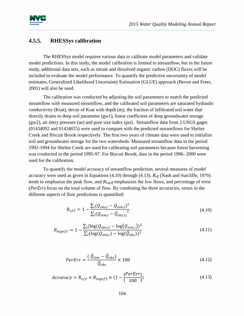
2015 Water Quality Modeling Annual Report
104
4.5.5. RHESSys calibration
The RHESSys model requires various data to calibrate model parameters and validate
model predictions. In this study, the model calibration is limited to streamflow, but in the future
study, additional data sets, such as nitrate and dissolved organic carbon (DOC) fluxes will be
included to evaluate the model performance. To quantify the predictive uncertainty of model
estimates, Generalized Likelihood Uncertainty Estimation (GLUE) approach (Beven and Freer,
2001) will also be used.
The calibration was conducted by adjusting the soil parameters to match the predicted
streamflow with measured streamflow, and the calibrated soil parameters are saturated hydraulic
conductivity (Ksat), decay of Ksat with depth (m), the fraction of infiltrated soil water that
directly drains to deep soil parameter (gw1), linear coefficient of deep groundwater storage
(gw2), air entry pressure (ae) and pore size index (psi). Streamflow data from 2 USGS gages
(01434092 and 01434025) were used to compare with the predicted streamflows for Shelter
Creek and Biscuit Brook respectively. The first two years of climate data were used to initialize
soil and groundwater storage for the two watersheds. Measured streamflow data in the period
1992-1994 for Shelter Creek are used for calibrating soil parameters because forest harvesting
was conducted in the period 1995-97. For Biscuit Brook, data in the period 1996- 2000 were
used for the calibration.
To quantify the model accuracy of streamflow prediction, several measures of model
accuracy were used as given in Equations (4.10) through (4.13). Reff (Nash and Sutcliffe, 1970)
tends to emphasize the peak flow, and Rlogeff emphasizes the low flows, and percentage of error
(PerErr) focus on the total volume of flow. By combining the three accuracies, errors in the
different aspects of flow predictions is quantified:
𝑅𝑒𝑓𝑓 = 1 −∑ (𝑄𝑜𝑏𝑠,𝑖 − 𝑄𝑠𝑖𝑚,𝑖)
2𝑖
∑ (𝑄𝑠𝑖𝑚,𝑖 − �̅�𝑜𝑏𝑠,𝑖)2
𝑖
(4.10)
𝑅𝑙𝑜𝑔𝑒𝑓𝑓 = 1 −∑ (log(𝑄𝑜𝑏𝑠,𝑖) − log(𝑄𝑠𝑖𝑚,𝑖))
2𝑖
∑ (log(𝑄𝑠𝑖𝑚,𝑖) − log(�̅�𝑜𝑏𝑠))2𝑖
(4.11)
𝑃𝑒𝑟𝐸𝑟𝑟 =(�̅�𝑠𝑖𝑚 − �̅�𝑜𝑏𝑠)
�̅�𝑜𝑏𝑠
× 100 (4.12)
𝐴𝑐𝑐𝑢𝑟𝑎𝑐𝑦 = 𝑅𝑒𝑓𝑓 × 𝑅𝑙𝑜𝑔𝑒𝑓𝑓 × (1 − |𝑃𝑒𝑟𝐸𝑟𝑟
100|) (4.13)

4. Model Development and Applications
105
where Qobs,i is the observed streamflow and Qsim,i is the simulated flow at any given time step (i),
and and are the average of daily streamflow.
Figure 4.59 shows the preliminary calibration results for Shelter Creek and Biscuit
Brook. For Shelter Creek, the model underestimated the peak flow, and failed to reproduce some
small peaks. However, the model successfully captured the observed flow recession. The flow
accuracy measures using Equations (4.10) through (4.13) reflect this pattern; Reff had lower value
(0.46) than Rlogeff (0.65) (Table 4.14). For Biscuit Brook, the model had lower flow accuracy
compared with those for Shelter Creek. The model also underestimated peak flow, and showed
better prediction of low flows (Rlogeff =0.54) that those of high flows (Reff =036). For the two
watersheds, the high error in peak flow may be related to the uncertainty of precipitation input
data and snow prediction. Tang et al. 2014 showed that using the data from 10 Cooperative
Observer Program stations (COOP) has better streamflow prediction for Biscuit Brook; Reff
values range from 0.58 to 0.61. The uncertainty of soil depth data may be a potential source for
error in the peak flow prediction. Compared with Shelter Creek, Biscuit Brook had higher
percentage error in flow. The assumption that LAI is spatially uniform may also contribute to
this error.

2015 Water Quality Modeling Annual Report
106
Figure 4.59. Streamflow calibration for Shelter Creek and Biscuit Brook watershed: (a) Shelter
Creek watershed, and (b) Biscuit Brook watershed

4. Model Development and Applications
107
Table 4.14. Accuracy of Streamflow predictions for the Shelter Creek Watershed and
the Biscuit Brook watershed
Watershed Reff Rlogeff PerErr Accuracy
Shelter Creek 0.46 0.65 -11.9 0.26
Biscuit Brook 0.36 0.54 -5.6 0.19
4.5.6. Conclusions and future plans
This study shows the initial results of streamflow predictions using RHESSys, and the
estimates of vegetation indices (SR, NDVI, ISR and LAI) using Landsat TM imagery. Simulated
streamflow results suggest a necessity for improving climate inputs, soil parameters and
vegetation parameters. In future work, various remote sensing data (Landsat-TM, LIDAR and
MODIS) will be included to improve the vegetation parameters (LAI, vegetation species, and
phenology parameters of deciduous forests). In addition, the current model used the daily
precipitation and air temperature data from the Slide Mountain climate station that is far from
Shelter Creek and Biscuit Creek. Using these data results in higher uncertainty in the climate
input for RHESSys modeling. Future work will improve the climate input data by combining the
available climate station data with PRISM data. Current model calibration is limited to
measured streamflow data. Soil and stream biogeochemistry data (nitrate and DOC) will be
included in future model calibration. The predictability of forest recovery in the Shelter Creek
watershed after the forest harvesting will be tested. Forest recovery data can be estimated using
the vegetation indices (NDVI, LAI, etc.) derived from Landsat imagery data. The predicted LAI
using the calibrated model will be compared with the estimated forest recovery data. It is
expected that using these additional data will improve model parameterizations and predictions.
The improved model will be used to test the impact of climate change and forest disturbance on
flow, ET, and nitrate and DOC fluxes.

2015 Water Quality Modeling Annual Report
108

5. Data Analysis to Support Modeling
109
5. Data Analysis to Support Modeling
5.1. West of Hudson Reservoir Water Budgets, 2000-2015
In order to form a basis for data analysis and water quality modeling of the West of
Hudson (WOH) reservoirs for the entire period of water quality monitoring, DEP has been
working to compute water budgets for all of the WOH reservoirs. Here we describe the general
procedure used to compute these water budgets, and the results for Delaware system reservoirs
(Cannonsville, Pepacton, Neversink, and Rondout) for the period 2000 through 2015 are
presented.
A water volume conservation equation for a reservoir may be expressed as
EPAQQQQ
dt
dVSOGIUIG (5.1)
where V is the reservoir volume (storage), t is time, QIG is the gaged surface inflow, QIU is the
ungaged surface inflow, QO is the total outflow (sum of drinking water withdrawal, spill, and
dam releases), AS is the surface area of the reservoir, and P and E are the precipitation directly
onto and evaporation from the surface of the reservoir.
All of the reservoirs have at least one gaged tributary, with discharge measurements
available from USGS. A list of USGS stream gages in the WOH watersheds are shown in Table
5.1; note that this table does not list gages that are upstream of other gages in a particular
watershed. For Ashokan and Neversink, one USGS gage determines the gaged reservoir inflow;
there are two gages for Cannonsville and Rondout, three for Schoharie, and four for Pepacton.
The ungaged watershed areas as a percentage of the total watershed area is in the range of 22 to
38 percent for WOH, with the exception being Schoharie, where only 6% of the watershed is
ungaged.

2015 Water Quality Modeling Annual Report
110
Table 5.1. U.S. Geological Survey (USGS) stream gaging and reservoir elevation stations in the
West of Hudson reservoirs. Stream gaging stations that are upstream of other stations are not
included. USGS gage remarks refer to accuracy of stream gaging observations.
Drainage Average USGS % of
Reservoir and USGS Gage Area Flow Gage area
mile2 MGD Remarks ungaged
Ashokan Reservoir (AS= 7800 acres)
Esopus Creek at Coldbrook 192 Good
Ashokan Reservoir 256 - 25.0
Esopus Creek near Lomontville 279 Fair
Cannonsville Reservoir (AS= 5260 acres)
W.Branch Delaware R. at Walton 332 394 Good
Trout Creek at Trout Cr. 20.2 24 Fair
Cannonsville Reservoir 454 - 22.4
W. Branch Delaware R. at Stilesville 456 407 Fair
Neversink Reservoir (AS= 1430 acres)
Neversink River at Claryville 66.6 127 Fair
Neversink Reservoir 92.5 - 28.0
Neversink River at Neversink 92.6 44 Good
Pepacton Reservoir (AS= 4940 acres)
E. Branch Delaware R. at Margaretville 163 205 Good
Mill Brook 25.2 37 Fair
Tremper Kill 33.2 39 Fair
Platte Kill 34.9 45 Good
Pepacton Reservoir 372 - 31.1
E. Branch Delaware R. at Downsville 372 156 Good
Rondout Reservoir (AS= 2060 acres)
Rondout Creek near Lowes Corners 38.3 67 Fair
Chestnut Creek at Grahamsville 20.9 Fair
Rondout Reservoir 95.4 - 37.9
Rondout Creek at Rosendale 383 Good
Schoharie Reservoir (AS= 1140 acres)
Schoharie Creek at Prattsville 237 366 Fair
Manor Kill at W. Conesville 32.4 35 Fair
Bear Kill near Prattsville 25.7 30 Fair
Schoharie Reservoir 315 - 6.3
Schoharie Creek at Gilboa 316 304 Fair

5. Data Analysis to Support Modeling
111
Similarly, QO is the total reservoir outflow, which is the sum of drinking water
withdrawal, release of water through the base of the dam to the stream channel downstream, and
spill. The precipitation term P is the rate of precipitation (depth/time) falling directly onto the
water surface of the reservoir, while E is a similar term representing evaporation from the
reservoir water surface.
The magnitude of the precipitation and evaporation terms can be estimated using
Cannonsville Reservoir (surface area AS=5260 acres) as an example. Using annual average
precipitation and evaporation rates of 45 and 30 inches per year yields the following estimates
for corresponding terms in Equation (5.1): P AS 17 MGD, E AS 12 MGD, and net
(P – E) AS 7 MGD, which is about 2% of the average annual gaged inflow at Cannonsville
(418 MGD; Table 5.1). Given the accuracy of the streamflow gaging measurements for gages
classified as fair or good (Table 5.2), the magnitude of the precipitation/evaporation term is
smaller than errors likely to be present in QIG. Regarding the net groundwater inflow/outflow
term QG, there is little basis for estimating this term individually for any of the WOH basins, and
it is assumed to be negligibly small relative to QIG and QO. As a result, the precipitation,
evaporation, and groundwater terms in Equation (5.1) are neglected, so that their value is
effectively lumped into the calculation of QIU. The resulting water balance equation used here is
then
OIUIG QQQ
dt
dV (5.2)
This equation was applied to Cannonsville Reservoir by Owens (1998) in order to determine the
ungaged inflow QIU from observations of QIG, QO, and reservoir water surface elevation for
1995, and is used here.
Table 5.2 Descriptors of accuracy of USGS streamflow measurements (included
in USGS documents in “Remarks” section).
USGS Gage
Description
Accuracy
Excellent 95% if data within 5% of true value
Good 95% if data within 10% of true value
Fair 95% if data within 15% of true value
Poor Less than Fair

2015 Water Quality Modeling Annual Report
112
This calculation procedure is based on daily average observations of QIG and QO, and
daily observations of the reservoir water surface elevation. From bathymetric curves or tables,
values of the reservoir storage volume V are determined from water surface elevation, or vice
versa. The subscript i associated with V, QIG, QIU, and QO represents the value on day i. Using
daily values of the reservoir storage volume, there are three simple alternative ways to
approximate the time derivative in Equations (5.1) and (5.2). These are:
Forward difference:
t
VV
dt
dV ii
i
1 (5.3)
Centered difference:
t
VV
dt
dV ii
i
2
11 (5.4)
Backward difference:
t
VV
dt
dV ii
i
1 (5.5)
where the time interval t is the time interval of calculations, which here is 1 day. Water
volume calculations were performed for each of these 3 alternative approximations. With these
alternative approximations for dV/dt, the following Equation (5.2) is used to solve for daily
values of the ungaged inflow QIU.
iOiIG
i
iIU QQdt
dVQ
(5.6)
Application of Equation (5.6) to a dataset of observations intermittently leads to the result that
iIUQ is negative. This occurs due to errors in the quantities on the right side of Equation (5.6).
Since we are describing this quantity as an ungaged inflow, a negative value is not realistic. As a
result, a modified version of Equation (5.6) is used. An error term is introduced into the water
balance, where errors occur due to the constraint that iIUQ 0. The following procedure is
used:

5. Data Analysis to Support Modeling
113
if
1iiOiIG
i
EQQdt
dV 0 then:
1iiOiIG
i
iUI EQQdt
dVQ , and
Ei = 0
_________________________________________________
else if
1iiOiIG
i
EQQdt
dV < 0 then:
0iUIQ , and
1iiOiIG
i
i EQQdt
dVE
(5.7)
This computational procedure begins with the initial error E0=0. When applied, this
procedure may lead to the result that 0iUIQ and the error is non-zero for a single isolated day.
In other cases, iUIQ may be set to zero for a number of consecutive days, and the error in the
water balance that results will accumulate over that period. For all cases for which the procedure
was applied here, (Cannonsville, Neversink, Pepacton, and Rondout for 2000 through 2015), a
water balance with nonzero error persists for no more than a week or two, and the impact of the
accumulated error on the water surface elevation is small.
An example of the application of this procedure is shown in Figure 5.1, where
components of the water budget equations are shown for the period of February 20 through
March 20, 2000 at Cannonsville. For the period Feb. 20 through 27, nonzero values of the
ungaged inflow (blue line) are computed and the error is zero. On Feb. 28, a negative value of
ungaged inflow is computed from the basic water balance; this ungaged inflow is set to zero and
a nonzero error is computed. Zero values of ungaged inflow, and nonzero error continues until
March 11, when a balance without error is established.

2015 Water Quality Modeling Annual Report
114
Figure 5.1. Example of water budget calculation for Cannonsville for Feb. 21 to March 20,
2000: (a) components of the budget calculation, and (b) resulting error in water
surface elevation.
To investigate the effect of errors, the computed time series of ungaged inflow is then
used together with the observed time series of gaged inflow and total outflow in a prediction of
storage volume, using the following predictive form of the water budget equation:
(a)
Wa
ter
Vo
lum
e,
MG
-2000
0
2000
4000
6000
8000
Volume Gaged InflowOutflowUngaged InflowError
(b)
2/21/2000 2/28/2000 3/6/2000 3/13/2000 3/20/2000
Err
or
in E
leva
tio
n,
fee
t
-0.02
0.00
0.02
0.04
0.06

5. Data Analysis to Support Modeling
115
iOiIUiIGii QQQtVV 1 (5.8)
During periods when there is no error in the balance (Ei = 0), the volume computed from
Equation (5.8), and the associated water surface elevation exactly match observations; the use of
the water balance equation to compute the ungaged inflow ensures this result. However, when
nonzero errors exist, the volume from Equation (5.8), and the associated water surface elevation,
are greater than the observations. The maximum value of the error in water surface elevation
and summarized below.
Regarding the three alternatives for approximating the dV/dt term in the water balance
equation (Equations (5.3) through (5.5), the forward difference approximation gave the smallest
errors, only slightly smaller than the centered difference approximation, while the backward
difference approximation produced substantially larger errors. As a result, the forward
difference approximation (5.3) was used in all water budget calculations presented here.
The application of this procedure to Cannonsville for the 16-year period of 2000 through
2015 is summarized in Table 5.3. On average, the annual computed ungaged volume was 15.5%
of the total (gaged and ungaged) volume. There were periods during each of the 16 years where
the errors in the water balance were introduced as described above. However, the resulting
maximum error in predicted water surface elevation during any individual year was generally
less than 0.1 feet, with a maximum for the 16-year period of 0.13 feet. The time series of
observed gage inflow (sum of West Branch Delaware River and Trout Creek) and computed
ungaged inflow for 2015, and the error in computed reservoir water surface elevation determined
from application of Equation (5.8), are shown in Figure 5.2.
Similar tabular summaries of the application of this water balance procedure for 2000-
2015, and predictions and water surface elevation errors for 2015, are presented for Neversink
(Table 5.4 and Figure 5.3), Pepacton (Table 5.5 and Figure 5.4), and Rondout Reservoirs (Table
5.6 and Figure 5.5). Note that the total gaged inflow at Rondout is the sum of USGS discharge
measurements for Rondout and Chestnut Creeks, and DEP observations of aqueduct flows from
Cannonsville, Neversink, and Pepacton.
The ungaged watershed area as a percentage of the total (gaged plus ungaged) watershed
area for each of the 4 reservoir watersheds is shown in Table 5.7 together with the ungaged
reservoir inflow as a percentage of the total (gaged plus ungaged) inflow for 2000-2015. In all
cases, the ungaged percentage of total inflow is less than the ungaged percentage of total
watershed area. This leads to the conclusion that in terms of streamflow generated per unit
watershed area, ungaged areas generate less streamflow that the gaged portions of the watershed.

2015 Water Quality Modeling Annual Report
116
Table 5.3. Annual water balance calculations for Cannonsville Reservoir, 2000
through 2015. Change in storage over the year and total annual inflow and
outflow volumes are in billion gallons (BG).
Year
Change in
Storage
Gaged
Inflow
Outflow
Ungaged
Inflow
Ungaged
% of Total
Inflow
Max. Error
Water Surf.
Elev., feet
2000 27 195 198 31.1 13.8 0.07
2001 -87 94 202 21.1 18.4 0.06
2002 75 159 117 33.6 17.5 0.03
2003 15 245 264 32.3 11.7 0.08
2004 -1 190 224 32.6 14.6 0.05
2005 -9 180 235 46.4 20.6 0.02
2006 4 243 305 65.2 21.3 0.08
2007 2 202 233 32.6 13.9 0.08
2008 2 216 250 35.7 14.2 0.09
2009 -9 178 221 34.2 16.2 0.07
2010 -1 192 219 26.0 11.9 0.13
2011 4 300 340 43.9 12.8 0.13
2012 -9 127 158 22.3 15.0 0.02
2013 5 178 196 22.7 11.4 0.08
2014 -24 145 206 36.4 20.1 0.02
2015 16 136 151 30.8 18.5 0.01
2000-15 4 2972 3515 547 15.5 0.13
Figure 5.2. Cannonsville water budget results, 2015: (a) error in predicted water surface
elevation, and (b) gaged and ungaged inflows.
(b)
Inflow
, 10
6 g
al/day
0
1000
2000
3000
4000
5000Total Gaged Ungaged
Jan Feb Mar Apr AugMay Jun Jul Sep Oct Nov Dec
(a)
Ele
v. E
rror,
ft
0.000
0.001
0.002
0.003

5. Data Analysis to Support Modeling
117
Table 5.4. Annual water balance calculations for Neversink Reservoir, 2000
through 2015. Change in storage over the year and total annual inflow and
outflow volumes in billion gallons (BG).
Year
Change in
Storage
Gaged
Inflow
Outflow
Ungaged
Inflow
Ungaged
% of Total
Inflow
Max. Error
Water Surf.
Elev. meter
2000 14 56 54 12.1 17.7 0.007
2001 -17 33 57 6.7 17.2 0.017
2002 15 41 35 8.1 16.4 0.013
2003 7 74 86 20.1 21.5 0.011
2004 -3 59 78 17.0 22.4 0.031
2005 1 60 77 19.0 24.1 0.024
2006 0 62 77 13.9 18.2 0.016
2007 -4 50 64 10.9 17.9 0.015
2008 5 63 71 13.5 17.7 0.015
2009 -3 57 73 12.6 18.0 0.009
2010 -1 57 68 9.8 14.7 0.051
2011 5 82 105 28.9 26.1 0.018
2012 -1 48 65 16.5 25.6 0.006
2013 -1 43 58 13.2 23.4 0.010
2014 -4 50 62 7.4 12.9 0.011
2015 4 45 48 6.9 13.1 0.009
2000-15 17 880 1079 216 19.7 0.051
Figure 5.3. Neversink water budget results, 2015: (a) error in predicted water surface
elevation, and (b) gaged and ungaged inflows.
(b)
Inflow
, 10
6 g
al/day
0
200
400
600
800
Total Gaged Ungaged
Jan Feb Mar Apr AugMay Jun Jul Sep Oct Nov Dec
(a)
Ele
v. E
rror,
ft
0.000
0.002
0.004
0.006
0.008
0.010

2015 Water Quality Modeling Annual Report
118
Table 5.5. Annual water balance calculations for Pepacton Reservoir, 2000
through 2015. Change in storage over the year and total annual inflow and
outflow volumes in billion gallons (BG).
Year
Change in
Storage
Gaged
Inflow
Outflow
Ungaged
Inflow
Ungaged
% of Total
Inflow
Max. Error
Water Surf.
Elev. meter
2000 16 157 177 35.6 18.5 0.005
2001 -65 85 172 20.9 19.7 0.014
2002 61 126 96 31.1 19.8 0.012
2003 25 219 243 50.3 18.7 0.002
2004 0 162 183 30.0 15.6 0.055
2005 -14 160 203 19.2 10.7 0.036
2006 4 195 240 48.6 19.9 0.014
2007 -3 172 216 41.4 19.4 0.002
2008 12 183 209 37.6 17.0 0.005
2009 -10 131 183 41.9 24.2 0.001
2010 -4 166 205 35.8 17.7 0.007
2011 13 245 285 52.4 17.6 0.006
2012 -26 108 167 32.6 23.2 0.002
2013 6 135 161 32.2 19.2 0.003
2014 -19 132 184 33.6 20.3 0.003
2015 11 106 117 21.1 16.6 0.003
2000-15 7 2483 3040 564 18.5 0.055
Figure 5.4. Pepacton water budget results, 2015: (a) error in predicted water surface elevation,
and (b) gaged and ungaged inflows.
(b)
Inflow
, 10
6 g
al/day
0
500
1000
1500
2000
2500
3000Total Gaged Ungaged
Jan Feb Mar Apr AugMay Jun Jul Sep Oct Nov Dec
(a)
Ele
v. E
rror,
ft
0.000
0.001
0.002
0.003
0.004

5. Data Analysis to Support Modeling
119
Table 5.6. Annual water balance calculations for Rondout Reservoir, 2000
through 2015. Change in storage over the year and total annual inflow and
outflow volumes in billion gallons (BG).
Year
Change in
Storage
Gaged
Inflow
Outflow
Ungaged
Inflow
Ungaged
% of Total
Inflow
Max. Error
Water Surf.
Elev. meter
2000 -1 256 283 26.1 9.2 0.008
2001 1 261 271 11.3 4.2 0.018
2002 1 210 226 16.9 7.5 0.019
2003 1 215 238 23.9 10.0 0.011
2004 1 239 260 22.3 8.5 0.003
2005 -1 240 262 21.5 8.2 0.018
2006 0 192 212 18.9 8.9 0.039
2007 -2 241 258 14.9 5.8 0.019
2008 1 197 217 20.8 9.6 0.009
2009 0 219 234 15.2 6.5 0.027
2010 1 248 262 14.8 5.6 0.015
2011 0 261 289 28.7 9.9 0.009
2012 -1 261 277 14.7 5.3 0.011
2013 1 255 268 13.6 5.1 0.014
2014 -1 226 239 11.4 4.8 0.032
2015 1 210 221 12.0 5.4 0.010
2000-15 1 3731 4016 287 7.1 0.039
Figure 5.5. Rondout water budget results, 2015: (a) error in predicted water surface elevation,
and (b) gaged and ungaged inflows.
(b)
Inflow
, 10
6 g
al/day
0
200
400
600
800
1000Total Gaged Ungaged
Jan Feb Mar Apr AugMay Jun Jul Sep Oct Nov Dec
(a)
Ele
v. E
rror,
ft
0.0000.0020.0040.0060.0080.0100.012

2015 Water Quality Modeling Annual Report
120
Table 5.7. Comparison of computed ungaged inflow as a percentage of total
(gaged plus ungaged) inflow for the 16-year period, and the ungaged watershed
area as a percentage of the total (gaged plus ungaged) watershed area.
Reservoir
Ungaged % of
Total Inflow
Ungaged % of Total
Watershed Area
Cannonsville 15.5 22.4
Neversink 19.7 28.0
Pepacton 18.5 31.1
Rondout 7.1 37.9
5.2. Hydraulic Residence Time in West of Hudson Reservoirs
The hydraulic residence time in a reservoir is defined as the time period that a parcel of
water resides within the reservoir basin, beginning at inflow from a tributary stream until leaving
the basin through either drinking water withdrawal, dam release, or spill. The hydraulic
residence time is generally expected to be a function of the shape and bathymetry of the reservoir
basin, rates of inflow to and outflow from the reservoir, weather conditions, and thermal
stratification and mixing within the reservoir.
Even under steady inflow and outflow conditions and invariant weather, the residence
time experienced by individual parcels of water is variable due to turbulent transport and mixing
within the reservoir basin, and the variety in pathways by which a parcel can move through the
reservoir. These effects can be observed in a tracer experiment, where a quantity of a
conservative tracer (such as rhodamine dye) is released quickly into a reservoir inflow. If the
concentration of tracer is then measured over time in a reservoir outflow, such as drinking water
withdrawal, a curve generally like that shown in Figure 5.6 would be observed. This curve
generally indicates that some parcels of water are transported relatively quickly to the outflow
point, while other parcels travel more slowly. The hydraulic residence time identified from this
experiment would be equal to the elapsed time after release required for one-half of the tracer
mass to arrive at the outflow. For the NYC reservoirs that have multiple tributaries and
generally three different types and locations of outflow, the residence time varies for each pair of
inflow and outflow.

5. Data Analysis to Support Modeling
121
Figure 5.6. Typical or expected observation of dye tracer concentration in a reservoir outflow
in response to a quick release of tracer in a reservoir inflow.
Conducting such a dye tracer experiment is the only way to physically measure hydraulic
residence time. However, mathematical model simulations can be made to replicate this field
experiment. Model application to determine residence time is much more economical and
flexible, in that a range of environmental conditions (inflow and outflow rates, weather, reservoir
stratification) can be considered. However, the model must be validated under a range of such
conditions to ensure that predictions are a good representation of field conditions.
In the absence of such simulations, the residence time for a reservoir can be estimated by
assuming that the reservoir is completely mixed, and that plug flow occurs from reservoir inflow
to the outflow. Completely mixed conditions exist in the reservoirs only during spring and fall
turnover, when thermal stratification is absent. Plug flow assumes that individual parcels of
water entering the reservoir move from inflow to outflow like the individual cars that make up a
railroad train moving down the tracks; the parcels remain in the order at which they entered as
they move through the reservoir. The assumption of plug flow neglects dispersion in the
reservoir.
Under these assumptions, the reservoir residence time is equal to equal to V / QO, where
V is the reservoir volume and QO is the total rate of reservoir outflow. Of course, these quantities
Time after tracer release
Tra
ce
r C
on
ce
ntr
atio
n in
Ou
tflo
w
Time at which half of tracer masshas passed the outflow
Hydraulic Residence
Time

2015 Water Quality Modeling Annual Report
122
vary with time. In order to reduce the variability in the quantities, 1-year moving averages of V
and QO were computed from records of daily records of these quantities. For example, a 1-year
average of V for March 25, 2015 was computed by averaging daily values of V for March 26,
2014 through March 25, 2015.
Values of the 1-year moving average reservoir storage for the Catskill and Delaware
system reservoirs are shown in Figure 5.7 and Figure 5.8. Periods of significant reservoir
drawdown for both systems occurred in 1980-1981, 1985, and 2001-2002. Similarly, the 1-year
moving average values of reservoir outflow are shown in Figure 5.9 and Figure 5.10. Periods of
significant low flow are generally consistent with the noted drawdown periods. Unusually high
outflows occur when the spill is large, as occurred in the wet periods in 1976, 2006-2007, and
2011. The residence time, this being the quotient of volume and outflow, for the Catskill and
Delaware reservoirs is shown in Figure 5.11 and Figure 5.12. Statistics for the hydraulic
residence time for each reservoir over the entire 40 year record are given in Table 5.8. Despite
the relatively small variability in volume and particularly inflow, Rondout Reservoir displays a
coefficient of variation (ratio of standard deviation to the mean) that is similar to the other
reservoirs.
Table 5.8. Statistics for hydraulic residence time for Catskill and Delaware system reservoirs,
1966 through 2015. Mean and standard deviation in days.
Reservoir
Mean
Standard
Deviation
Coeff. of
Variation
Schoharie 39 8.5 0.22
Ashokan West 78 16 0.21
Ashokan East 123 26 0.21
Cannonsville 143 25 0.18
Neversink 162 29 0.18
Pepacton 250 40 0.16
Rondout 61 10 0.17

5. Data Analysis to Support Modeling
123
Figure 5.7. Storage in Catskill System Reservoirs, 1966 through 2015.
Figure 5.8. Storage in Delaware System Reservoirs, 1966 through 2015.
1968 1972 1976 1980 1984 1988 1992 1996 2000 2004 2008 2012 2016
Re
se
rvo
ir S
tora
ge
(B
G)
0
20
40
60
80
100
Schoharie
West Basin Ashokan
East Basin Ashokan
1968 1972 1976 1980 1984 1988 1992 1996 2000 2004 2008 2012 2016
Re
se
rvo
ir S
tora
ge
(B
G)
0
20
40
60
80
100
120
140
160
180
Rondout
Pepacton
Cannonsville
Neversink

2015 Water Quality Modeling Annual Report
124
Figure 5.9. Reservoir outflow for Catskill system reservoirs, 1966 through 2015.
Figure 5.10. Reservoir outflow for Delaware system reservoirs, 1966 through 2015.
1968 1972 1976 1980 1984 1988 1992 1996 2000 2004 2008 2012 2016
Re
se
rvo
ir O
utflo
w (
MG
D)
0
200
400
600
800
1000
Schoharie
West Basin Ashokan
East Basin Ashokan
1968 1972 1976 1980 1984 1988 1992 1996 2000 2004 2008 2012 2016
Re
se
rvo
ir O
utflo
w (
MG
D)
0
200
400
600
800
1000
1200
Rondout
Pepacton
Cannonsville
Neversink

5. Data Analysis to Support Modeling
125
Figure 5.11. Hydraulic residence time for Catskill System Reservoirs, 1966 through 2015.
Figure 5.12. Hydraulic residence time for Delaware system reservoirs, 1966-2015.
1968 1972 1976 1980 1984 1988 1992 1996 2000 2004 2008 2012 2016
Wa
ter
Re
sid
ence
Tim
e (
da
ys)
0
50
100
150
200
250
Schoharie Ashokan West BasinAshokan East Basin
1968 1972 1976 1980 1984 1988 1992 1996 2000 2004 2008 2012 2016
Wa
ter
Re
sid
ence
Tim
e (
da
ys)
0
100
200
300
400
500
Rondout
Pepacton
Cannonsville
Neversink

2015 Water Quality Modeling Annual Report
126

6. Model Data Acquisition and Organization
127
6. Model Data Acquisition and Organization
6.1. GIS Data Development for Modeling
6.1.1. Water Quality Monitoring Sites
In 2015, the Water Quality Modeling Section’s GIS data library was updated with
additions to water quality monitoring sites and biomonitoring sites. These locations were
georeferenced from site descriptions provided by data samplers as part of the DEP’s LIMS
database entry. DEP snow monitoring and snow pillow locations data were updated with revised
information provided by DEP’s Operations Directorate.
6.1.2. Support for modeling projects
GIS support was provided to Water Quality Modeling Section staff, CUNY Postdoctoral
researchers, as well as other DEP staff in the Division of Water Quality Science and Research.
This support included the production and revision of maps included in the 2015 FAD Summary
and Assessment Report, the 2015 update to the Watershed Water Quality Monitoring Plan, and
conference presentations and posters.
Table 6.1 lists the types of GIS data used by the Water Quality Modeling Section. While
GIS data is used in virtually all DEP reservoir and watershed models, a particular area of use in
2015 was the support of application of two terrestrial (watershed) models: RHESSys and SWAT.
RHESSys applications include information derived from LiDAR data collected by DEP. The
LiDAR data, along with remote sensing images, are being compiled and analyzed for the
Neversink watershed to identify the spatial variation of canopy height and leaf area index (LAI)
that is used by RHESSys.
DEP’s Operations Directorate has been involved in application of the Army Corps of
Engineers HEC-RAS (River Analysis System) model to address questions related to cold water
releases from Cannonsville Reservoir to the downstream West Branch Delaware River. The
HEC-RAS model has been applied to this river channel to simulate the effect of channel
morphology changes on downstream river temperatures. To generate a geometric description of
the river channel for use in this model, input data were generated using HEC-GeoRAS using
available stream networks, elevation and cross section data. This work will continue to 2016 to
inform planning decisions.

2015 Water Quality Modeling Annual Report
128
Table 6.1. Inventory of GIS data used in water quality modeling.
Data Type Data Source Data Description Dates Modeling Needs
LiDAR DEP Tree height, canopy fraction
and LAI 2009
RHESSys Model
Input
DEM
(1 meter) DEP
Watershed delineation,
topographic parameters 2009
Watershed
delineation
Land Use/
Land Cover DEP
Spatial extent of types of land use
and land cover 2009
SWAT Model
Input
SSURGO2
Soil Survey USDA
Soil Characteristics, Percent Clay,
Ksat, Ksattop, Available Water
Content, Depth to Water Table,
2012 SWAT Model
Input
Aerial
Imagery
USGS Landsat TM multispectral
imagery
1990-
current
Leaf area index
(LAI) values and
tree phenology
NASA MODIS multispectral imagery 2002-
current
LAI, and tree
phenology
Forest Stands DEP, USFS Forest spatial extent 2009 RHESSys
Model Input
Vegetation
Cary Institute
of Ecosystem
Studies
Spatial extent of 11 vegetation
species 1986-1993
RHESSys
Model Input
6.2. Ongoing Modeling/GIS Projects
6.2.1. Reservoir Bathymetry Surveys
Accurate, current bathymetry data are required for modeling water quantity and quality of
NYC reservoirs. Last surveyed in the late 1990’s, the 6 WOH reservoirs are being re-surveyed
by the USGS through an Intergovernmental Agreement signed in 2013. The USGS will produce
GIS surface models of the reservoir bottoms, 2-foot elevation contours and an updated elevation-
area-capacity table for each reservoir. Work continued in 2015 on the processing of data
collected for the 6 WOH reservoirs. All fieldwork had been completed, and select draft data
were delivered to DEP in 2014. The USGS contractors have been processing all reservoir data in
parallel in order to deliver a complete set of draft data for review in early 2016.

6. Model Data Acquisition and Organization
129
To further improve reservoir data and provide additional information to the Modeling
Section, DEP is reviewing a proposed scope of work to conduct new bathymetric surveys for the
13 EOH reservoirs and 3 controlled lakes. The draft scope of work was submitted by the USGS,
and will provide the same level of detail as the data being created for WOH. If approved, the
project will provide all data deliverables, including surface models, 2-foot elevation contours and
elevation-area-capacity tables to DEP no later than 2020.
6.2.2. Modeling Database Design
Historically, data used by the Water Quality Modeling Section are primarily stored and
classified by individual staff members to suit the needs of the specific models. An effort is
currently underway to centralize and standardize the storage of datasets to improve data
interoperability between all staff and associated researchers. Multiple software programs are
being evaluated to determine an optimal solution that will allow all modelers to access datasets.
The resulting database will include the capability to properly document the data, including the
data source, collection date, and identification of data used in models.
This effort will improve data access and reduce duplication of effort in the central
compilation of data with customized queries to provide appropriately formatted data files for
each staff member. An additional goal of the project is to create a warehouse to store and
document the data used to calibrate each model, and the results of model runs, including all key
datasets and parameters used. Maintaining these data will ultimately detail the lineage of the
models, and can aide in the interpretation of results. In some cases, data may be appropriately
stored in a relational database structure internally, but in others, such as time-series monitoring
data owned by other agencies, they will only be accessed as needed. A data curation solution
will be designed to support the variety of data access and management requirements as described
by the modeling group.
6.3. Time Series Data Development
An inventory of the necessary raw time series data for watershed and reservoir model
input and calibration is presented in Table 6.2 and Table 6.3, respectively. The time series data
includes meteorology, streamflow, water quality, and point source loads for watershed models.
For reservoir models the data includes meteorology, streamflow, stream, reservoir and key point
water quality and reservoir operations. Data sets are updated as new data become available. Lag
times between the current date and the dataset end dates are the result of QA/QC processes at the
data source and/or procurement timelines driving the acquisition of any purchased data.
In this reporting period, existing meteorological datasets being supplemented with
climate data from the PRISM climate model. PRISM data are calculated with 4 km2 resolution
grid cells, with variables including precipitation, min/max temperature and dew point. Data are

2015 Water Quality Modeling Annual Report
130
available from 1981-present, and were downloaded directly from the PRISM website
(http://prism.oregonstate.edu).
Table 6.2. Inventory of time-series data used for watershed modeling.
Data Type Data Source Data Description Dates* Modeling
Needs
Meteorology
Northeast
Regional
Climate Center
Daily Precipitation and
Max/Min Temperature
Pre 1960-
2013 Model Input
PRISM Climate Data 2004 Model Input
Wastewater
Treatment
Plants
DEP Monthly WWTP Nutrient
Loads 1990-2009 Model Input
Streamflow USGS Daily and Instantaneous
Streamflow
Period of
record
available
online via
USGS
Hydrology
Calibration /
Nutrient and
Sediment Loads
Water Quality DEP Routine and Storm Stream
Monitoring
Period of
record
avail. via
LIMS
Nutrient and
Sediment Loads
for Water
Quality
Calibration
NYSDEC** Stream Monitoring at West
Branch Delaware River
1992-2010
w/ recent
years
avail. via
LIMS
Nutrient and
Sediment Loads
for Water
Quality
Calibration
*Dates represent total span for all data sets combined. Individual station records vary.
**Now part of the DEP Water Quality dataset.

6. Model Data Acquisition and Organization
131
Table 6.3. Inventory of time-series data used for reservoir modeling.
Data Type Data
Source Data Description Dates*
Modeling
Needs
Meteorology DEP
Air Temperature, Relative
Humidity, Solar Radiation, PAR,
Wind Speed, Wind Direction, and
Precipitation
1994-June, 2010
Period of record
avail. Operations
Model Input
Keypoint and
Reservoir
Operations
DEP
Tunnel Water Quality, Flow and
Temperature; Reservoir Storage,
Spill, Withdrawal, and Elevation
Period of record
avail. via LIMS Model Input
Streamflow USGS Daily and Instantaneous
Streamflow
Period of record
available online
via USGS
Model Input
Stream
Hydrology DEP
Stream Water Quality, Flow and
Temperature
Period of record
avail. via LIMS Model Input
Limnology DEP Reservoir Water Quality, and
Temperature Profiles
Period of record
avail. via LIMS Model Input
*Dates represent total span for all data sets combined. Individual station records vary.

2015 Water Quality Modeling Annual Report
132

7. Modeling Program Collaboration
133
7. Modeling Program Collaboration
7.1. Water Research Foundation Project 4422 – Advanced Techniques
for Monitoring Changes in NOM and Controlling DBPs Under
Dynamic Weather Conditions
The goals of this project were to develop and test the effectiveness of on-line (in-situ)
monitoring tools that can detect changes in the character and amount of natural organic matter
(NOM), and associated disinfection byproducts under typical operating conditions, extreme
weather events, and future climate condition scenarios. Most of the work involved the
evaluation of advanced on-line instrumentation which utilizes ultraviolet (UV) absorbance and/or
fluorescence spectral measurements to detect changes in the concentration and chemical
character of NOM and associated formation potential for disinfection byproducts.
To achieve these goals, water samples were collected from various DEP reservoirs and
analyzed for a number of parameters including DBP formation potential, ultraviolet-visible light
absorbance using both laboratory and field instruments, and laboratory fluorescence
measurements. Formation potential measurements included the regulated total trihalomethanes
and haloacetic acid components as well as unregulated components including acetonitriles and
haloketones. XAD fractionation and polarity rapid assessment method (PRAM) were used to
separate and characterize NOM.
This work was completed in 2015, with the final report release in early 2016. This study
confirms that ultraviolet-visible spectroscopy and fluorescence can be a useful surrogate for
natural organic material and disinfection byproducts. Field instruments that can produce high-
quality data with minimal maintenance are commercially available. Application of these
instruments can provide additional information to utilities such as DEP with respect to formation
potential, thus allowing operations to be modified in response. However, the results indicate that
the optical measurements do not capture all of the potential variability in formation potential, and
that further study is needed to identify appropriate surrogate measures for formation potential
that cannot be measured with ultraviolet-visible light absorbance or fluorescence. In addition,
reservoir-specific models may need to be developed in order to refine decision making about the
optimal selection of individual water sources.
This project was completed by researchers from Hazen and Sawyer Engineers, and the
Department of Civil and Environmental Engineering at the University of Massachusetts, with
sponsorship by NYCDEP and WRF.

2015 Water Quality Modeling Annual Report
134
7.2. Water Research Foundation Project 4590 - Wildfire Impacts on
Drinking Water Treatment Process Performance: Development of
Evaluation Protocols and Management Practices
NYCDEP is one of six water utilities (the others being Denver Water, City of
Westminster Colorado, San Francisco Public Utilities, Truckee Meadows Water Authority, and
Metropolitan Water District of Southern California) participating in this WRF study, which is
now in its second year. Given the anticipated effect of climate change on frequency and
intensity of wildfires, this study is evaluating the effects of wildfires on forested watersheds,
including water quantity and availability, and water quality. The project will develop a
laboratory-based burn procedure to simulate the effects of wildfire on water quality and
treatability.
A literature review will be conducted to document how wildfires have changed water
quality, including particulates, nutrients, metals, and organic matter. The six participating
utilities will supply historic data from their watersheds regarding the impact of fires. Samples
will be collected to monitor the impact of previous wildfires, and the treatability of samples will
be evaluated. Compilation of these results will allow the site-specific implications to be
identified. The work is being conducted by researchers at the University of Colorado and Hazen
& Sawyer Consulting Engineers, and the project will be complete at the end of 2016.
7.3. Water Utility Climate Alliance (WUCA)
New York City DEP is one of ten large water utilities in the United States that form the
Water Utility Climate Alliance. This group was formed in order to identify, understand, assess
the impact of climate change, and to plan and implement programs to meet climate challenges.
WUCA members are involved in enhancing climate change research and improving water
management decision-making to ensure that water utilities will be positioned to respond to
climate change and protect our water supplies. Two white papers recently released by the Water
Utility Climate Alliance feature case studies of water utilities addressing the threat of climate
change, including DEP. These white papers advance understanding of how the relatively new
enterprise of climate change assessment and adaptation is developing.
DEP is also one of four WUCA utilities (New York, Tampa Bay, Seattle, and Portland)
participating in the Piloting Utility Modeling Applications (PUMA) project. In this program, the
four PUMA utilities have formed partnerships with scientific institutions to explore how to
integrate climate considerations into their specific programs for water quality and quantity
management. PUMA has convened workshops where water utility representatives and

7. Modeling Program Collaboration
135
researchers meet to discuss and compare approaches for addressing the impact of climate change
on water utilities. The four utilities pursued customized approaches based on specific utility
needs and learned important lessons in conducting assessments that may be of interest to the
wider adaptation community. In addition, these projects attempted to create a “climate services”
environment in which utility managers worked collaboratively and iteratively with climate
scientists to understand both utility concerns and the ability or limitations of today’s climate
science to respond to those concerns.
7.4. Global Lake Ecological Observatory Network (GLEON)
GLEON is a 10-year old organization that has been built around issues associated with
the setup and deployment of robotic buoys for observing physical and water quality conditions in
lakes and reservoirs, storage, processing, and analysis of the high-frequency data gathered by
such buoys, and use of the data in modeling. DEP staff have attended recent annual GLEON
meetings in Quebec and South Korea. DEP staff are also collaborating with other GLEON
members in the intervals between meetings, including sharing of selected data. This
participation has helped to ensure that DEP is getting the most out of its sizable investment in
robotic monitoring in the reservoirs and tributary streams. DEP has made use of GLEON
software tools in the analysis of robotic buoy data.
DEP is also applying the reservoir hydrothermal model GLM (General Lake Model) and
associated Aquatic Ecodynamics (AED) water quality model. These models are “open source”
software, and are thus open to use and revision by other researchers and professionals. These
models are currently being applied to Cannonsville and Neversink Reservoirs by one of the
CUNY postdoctoral researchers working in DEP’s Water Quality Modeling Section.
Several collaborations have developed from DEP’s participation in GLEON annual
meetings, where scientists meet to develop ideas and tools to analyze data from an array of lake
and reservoir sensors deployed around the globe to address local issues for individual aquatic
ecosystems. Additionally, this network of collaborators works to document changes in lake and
reservoir ecosystems that occur in response to different environmental conditions and stressors.
This is done in part by sharing and interpreting high-frequency sensor data and other water
quality and environmental data. DEP contributed data to four collaborative GLEON research
projects in 2015.

2015 Water Quality Modeling Annual Report
136
1. Temperature Sentinels in Northeastern North America (NENA): In-depth Study of
Lake Thermal Responses and Teleconnections in Northeastern North America
The primary intent of this study is to examine subsurface water temperature profiles from
lakes and reservoirs across the northeastern region of North America to determine how water
temperature responds to regional-scale climatic drivers and teleconnections. To accomplish this,
the researchers will examine a set of lakes and reservoirs with long-term, high resolution
temperature profile data and a larger set of NENA lakes and reservoirs with temperature profiles
from a single annual profile. Historical water temperature data for Cannonsville, Pepacton,
Neversink, and Rondout reservoirs at the deepest sites at the time of peak thermal stratification
were formatted and shared with the project lead scientist, Dr. David Richardson, SUNY New
Paltz for use in this GLEON-sponsored study.
2. GLEON Fellowship SALT project:
A study of increasing salinization of lakes and reservoirs was conducted as part of the
GLEON Fellowship Program in 2015. The Fellowship Program trains cohorts of graduate
students to explore the information contained in large data sets, work in diverse international
teams, and communicate their findings to a broad range of audiences. DEP contributed data for a
modeling analysis of global trends and drivers of lake and reservoir salinity to assess ecological
impacts. Data included specific conductivity, chloride, sulfate, and sodium concentrations for
the period of 1987 to 2014 for ten reservoirs, including Cannonsville, Pepacton, Neversink,
Schoharie, Boyds Corners, Cross River, Croton Falls, Middle Branch, New Croton, and Kensico.
The work was carried out in connection with the Cary Institute of Ecosystem Studies in
Millbrook, New York. The lead investigator was Dr. Hilary Dugan, a post-doctoral scientist at
the University of Wisconsin ̶ Madison.
3. Iron concentration trends around the globe
This project is an analysis of how iron concentrations in freshwaters around the world
have changed over the past 20 years. Data analysis is being performed by Caroline Björnerås, a
doctoral candidate at Lund University, Sweden, under the supervision of Dr. Emma
Kritzberg from Lund University and Dr. Gesa Weyhenmeyer, Uppsala University, Sweden. Data
contributed by DEP in 2015 included iron, total organic carbon, dissolved organic carbon, water
color, pH, sulfate, silica, dissolved oxygen, water temperature, and aluminum for two sites on
New Croton Reservoir for the period of 1994-2009.

7. Modeling Program Collaboration
137
4. Effects of Climate Change on Spring-Winter Runoff and Lake Productivity
The Climate Sentinels working group in GLEON is looking at the effects of ongoing
changes in the seasonality of winter – spring streamflow on lake productivity. The initial
hypothesis is: Changes in the timing of spring runoff, with more runoff occurring in the winter
and early spring, will lead to reduced productivity and phytoplankton biomass during the
summer stratified period. The foundation for this expectation is based on our current
understanding that nutrients delivered to a lake during colder, deeply mixed, and possibly ice
covered conditions, could be less effective at stimulating phytoplankton growth. To test the
hypothesis we are assembling data from a large variety of lakes that meet the following minimal
requirements:
In a geographic location where snow accumulation and melt significantly impact the
seasonality of stream discharge.
A lake or reservoir with data from 1990 or earlier and continuing to present. There should
be multiple samples per year that cover at least the period of thermal stratification.
Measurements of chlorophyll profiles during thermal stratification and/or measurements
of hypolimnetic oxygen at the onset and just before the loss of thermal stratification.
Stream discharge measurements of a major inflow to the lake starting in 1990 or earlier,
or measurements from a nearby stream or river than can be used to provide an index of
lake inflow.
Dr. Don Pierson, currently at Uppsala University, Sweden, is taking the lead with DEP data
contributed to the project.
5. Signal Processing Working Group
The GLEON Signal Processing working group has gathered profiling buoy data from 12
different lakes and reservoirs to assess subsurface dissolved oxygen and chlorophyll fluorescence
maxima across lake types. DEP has contributed 3 years (2009, 1010, and 2010) of robotic buoy
data from the west basin of Ashokan Reservoir to this project. This project is being coordinated
by Jennie Brentrup from Miami University of Ohio and Annie Scofield at Cornell University.

2015 Water Quality Modeling Annual Report
138
7.5. NYCDEP – City University of New York (CUNY) Modeling
Program
Through the reporting period, DEP has maintained a contract with the Research
Foundation of the City University of New York (RF-CUNY) that provides support for model and
data development by providing postdoctoral scientists who work with DEP water quality
modeling staff, and supporting research advisors. The work described in Sections 3.2, 4.1, 4.2,
and 4.5 of this report has been completed largely by CUNY postdoctoral research staff, working
together with their research advisors and staff of the Water Quality Modeling Section.
In August, 2014, a new 4-year contract was initiated between DEP and RF-CUNY.
Under this contract, RF-CUNY has hired four fulltime postdoctoral researchers who work in
DEP’s Water Quality Modeling office in Kingston, NY. Each of the researchers has an
associated research advisor who receive part-time support under this contract. The research that
has been initiated by these researchers continues to be a significant and critical component of
DEP’s modeling work. The postdoctoral program provides support in the form of providing
model development and application expertise, modeling software, and data sets and in three
project areas: (1) Evaluation of the effects of climate change on watershed processes and
reservoir water quality as a part of CCIMP; (2) evaluation of FAD programs and land use
changes on watershed processes and stream and reservoir water quality; and (3) development of
the modeling capability to simulate watershed loading of dissolved organic carbon (DOC), and
reservoir and water supply concentrations of DOC and disinfection byproduct formation
potential (DBPFP). At the end of 2015, all four postdoctoral positions were filled.
8. Modeling Program Scientific Papers and Presentations
139
8. Modeling Program Scientific Papers and Presentations
8.1. Published Scientific Papers
Mukundan, R., D. C. Pierson, E. M. Schneiderman, and M. S. Zion, 2015. Using detailed
monitoring data to simulate spatial sediment loading in a watershed. Environmental
Monitoring and Assessment, DOI 10.1007/s10661-015-4751-8
Abstract: The use of watershed models as cost-effective tools to quantify the impact of
conservation practices on water quality is often constrained by lack of data for model
parameterization. This study uses short-term (3 years) detailed monitoring data to guide spatially
distributed model parameterization and modeling analysis for suspended sediment in the Upper
Esopus Creek Watershed (UECW) that is part of the New York City water supply. The
calibrated Soil and Water Assessment Tool (SWAT) model simulated suspended sediment
loading from tributary sub-basins and at the watershed outlet that were comparable to field
measurements. Model simulations estimated that stream channels contributed the majority
(85%) of stream sediment in the study watershed followed by upland erosion (11%) and point
sources (4%), consistent with previous estimates and field observations. Long term (12 years)
simulation of the calibrated model was used to apportion the average annual sediment yields
from tributary sub-basins which ranged between 12 and 161 t km-2 year-1. Model simulations
were also used to understand the inter-annual variability and seasonality in suspended sediment
loading in the study watershed. We demonstrate the wider applicability of short-term detailed
monitoring for model parameterization and calibration, and long-term simulation of water quality
using the SWAT model.

2015 Water Quality Modeling Annual Report
140
8.2. Conference Presentations
Association for the Sciences of Limnology and Oceanography (ASLO)
Aquatic Sciences Meeting
February 22-27, 2015, Granada Spain
Simulating the effects of climate change on phytoplankton in a New York City
Water Supply Reservoir
Pierson, D. C., N. R. Samal, H. Markensten, and E. M. Owens
Abstract: The impacts of climate change on the phytoplankton in Cannonsville
Reservoir, a part of the New York City water supply, is evaluated using a coupled
watershed and reservoir modeling system, driven by downscaled climate scenarios
derived from CMIP3 climate models. The Generalized Watershed Loading Function
(GWLF) model simulates streamflow as well as dissolved and particulate nutrients,
which become inputs to a one dimensional reservoir model which includes the
PROTECH based phytoplankton functional group algorithms. Simulations predict that
there will be a future 10-15% increase in total chlorophyll during the period of thermal
stratification and that this increase will coincide with a reduction in the importance of
diatoms and an increasing importance of cyanobacteria. Average summer cyanobacteria
concentrations are simulated to increase by approximately 20% -70%. Model sensitivity
analysis suggests that it is largely the effects of climate change on reservoir thermal
structure as opposed to watershed loading that is responsible for the changes in
phytoplankton. These results are evaluated relative to previous changes in phytoplankton
associated with point and non-point source nutrient reductions.
Long term changes in ice seasons of twenty-one geographically distributed
freshwater lakes: Modeling Simulations and Observations
N. R. Samal, K. D. Jöhnk, D. C. Pierson, M. Leppäranta, H. Yao, B. R. Hargreaves, T.
Kratz, S. Sharma, A. Laas, D. Hamilton, R. Adrian, J. Rusak, D. Oezkundakci, C.
Williamson, D. Vachon, B. Denfeld, G. Kirillin, K. Czajkowski and L. Camarero
Abstract: Long term trends and variability in the seasonality of lake ice dynamics are
some of the clearest indicators of changes in climate conditions. The timing of ice
formation, ice cover duration and ice loss in lakes and reservoirs will modulate the
impact of regional weather conditions on lake thermal structure and mixing, and thus will
ultimately influence phytoplankton succession and trophic status of a lake. Here a simple
lake ice model that predicts lake ice timings and thickness has been applied to 21

8. Modeling Program Scientific Papers and Presentations
141
freshwater lakes and reservoirs around the globe. The model is driven by measurements
of air temperature and wind speed, as these are the most important factors influencing
formation and breakup. The effects of snowfall and solar radiation on ice characteristics
are not explicitly considered but can be parameterized. Even though the model does not
make detailed calculations of the ice cover energy budget it reproduces long-term trends
allowing for historical analysis of ice cover in these geographically distributed lakes.
Work of this ongoing GLEON project will include simple snow cover estimates derived
from precipitation and temperature data.
Gordon Research Conference and Seminar: Catchment Science
June 13-14, 2015
Andover, MA
Innovative Models for the Organic Carbon Budget of New York City (NYC)
Reservoirs.
Li, Y., K.E. Moore, R.Van Dreason, P.C. Hanson.
Abstract: In order to investigate the role of climate change in the carbon cycling of
aquatic systems, it is necessary to better understand organic carbon (OC) budgets at the
catchment scale. However, present studies on OC budgets are incomplete and uncertain
due to the complicated nature of cycling processes in lakes and reservoirs. This study
used the Framework for Aquatic Biogeochemical Models (FABM) to theoretically
explore the classic “Nutrient Phytoplankton Zooplankton Detritus” (NPZD) model for the
carbon cycling processes. Two NYC reservoirs with different catchment characteristics
were preliminarily examined to evaluate the role of allochthonous carbon and to
approximate the OC budgets for these reservoirs. This work will provide an improved
basis for water quality model structure, uncertainty analysis, and could ultimately lead to
improved modeling tools to help manage and plan for a regional water supply that serves
more than 9 million residents in NYC and upstate communities in a changing climate.

2015 Water Quality Modeling Annual Report
142
Gordon Research Conference and Seminar: Drinking Water Disinfection By-Products
August 8-14, 2015
South Hadley, MA.
Conceptual Model for Simulating Disinfection By-Products (DBPs) Precursors in
New York City (NYC) Reservoirs
Li, Y., R. Van Dreason., D.A. Smith K.E. Moore, P.C. Hanson, and E.M. Owens
Abstract: With more stringent regulatory requirements for disinfection byproducts
(DBPs) in drinking water by USEPA, it is important to better understand the origins of
DBP precursors in water supply systems. Due to the complex chemical characteristics
associated with DBP precursor origins, many DBP models are empirical and are unable
to identify the relative importance of autochthonous and allochthonous sources of DBP
precursors. This study used Cannonsville Reservoir, one of the NYC water supply
reservoirs, to preliminarily investigate algal-produced precursors compared to terrestrial
sources. Observed time series of nutrients (total phosphorus and nitrogen, TP and TN),
algal abundance (based on chlorophyll concentration), and organic matter (dissolved and
total organic carbon, DOC and TOC) during 1995-2014 illustrate long-term patterns of
the water quality variables that are commonly related to DBP formation. Furthermore,
the relationships between TN, OC, and DBP formation potential (DBPFP) were studied
in 2007 and 2008 to develop a conceptual model for studying algal-produced DOC as a
source of DBP precursors. This conceptual model will help in the development of
mechanistic models to simulate and potentially predict DBP precursors, with the ultimate
goal of understanding the potential changes in DBP precursors in the NYC water supply
under climate change.
The Occurrence of Dissolved Organic Carbon in the Catskill Mountain Watersheds
of the NYC Water Supply
R. Van Dreason, R. Mukundan
Abstract: An empirical model was recently developed by Mukundan and Van Dreason
(2014) that indicated that organic carbon concentration was the most important factor
explaining trihalomethane (THM) formation within the NYC distribution system. THMs
and other Disinfection by-products (DBPs) occur in drinking water as a result of a
reaction between organic matter naturally occurring in the water and the disinfectant (e.g.
chlorine) added to control microbial contaminants. THMs and other DBPs are a major
concern to water suppliers because of their suspected carcinogenic properties.

8. Modeling Program Scientific Papers and Presentations
143
Because of its important role in regulating DBP formation, in this presentation we will
describe the occurrence of DOC within the Catskill Mountain portion of NYC’s water
supply system. Regional and seasonal patterns will be compared using data collected
from the Catskill reservoirs. We also examine the patterns in DOC concentrations over
time, since increases in the reservoirs could have important ramifications on future DBP
formation in the distribution system.
NYC Watershed Science and Technical Conference
September 9, 2015
West Point, New York
Performance Assessment of Stochastic Weather Generators for Precipitation over
Catskill Mountain watersheds, New York, USA
Acharya, N., A. Frei, K.E. Moore, and J. Mayfield
Abstract: The New York City Department of Environmental Protection (DEP) has
performed studies to assess the potential impacts of climate change on the availability of
high quality water in this water supply system. To better address this, there is a need to
develop future climate scenarios that can be used as inputs to the DEP’s integrated suite
of hydrological models. There are two familiar approaches used to incorporate climate
change into vulnerability analyses viz., top-down and bottom-up approaches. Top-down
approaches use scenarios from Global Climate Models (GCMs). Bottom-up approaches
identify the climate vulnerabilities of a water supply system over a wide range of
potential climate changes. Stochastic weather generators are often employed in bottom-
up risk assessments to simulate potential shifts in both long-term (decadal) precipitation
means and persistence as well as in extreme daily precipitation amounts. The main goal
of the current work is to document the performance of two weather generators, the widely
used generator WGEN, and the comparatively new and sophisticated WeaGETS, in
simulating precipitation over the Catskill Mountain region. The performances of these
two weather generators are compared in order to assess their capabilities of reproducing
the observed statistical properties including the probability distributions, means and
variances, and the frequencies and magnitudes of extreme events.
Trends of Chlorophyll and Phytoplankton for New York City’s West of Hudson
Reservoirs (1988-2014)
Ray Homolac, NYCDEP

2015 Water Quality Modeling Annual Report
144
Abstract: The New York City Department of Environmental Protection (DEP) performs
limnology surveys on most of the water supply reservoirs and many water quality
monitoring parameters are analyzed. The historical record of DEP data will be examined
for long-term trends of chlorophyll a and total phytoplankton in the Catskill/Delaware
System reservoirs. An overview of the time period 1988 through 2014 will be presented
leading to a more in depth focus for 2004 through 2014.
Exploration and Evaluation of Long-Term Water Quality Data
Karen Moore, NYCDEP
Abstract: An important goal in watershed protection is to document changes in water
quality and look for linkages to what is occurring on the landscape. We applied statistical
methods including Weighted Regressions for Time, Discharge, and Season (WRTDS) to
the major inflows of New York City water supply West-of-Hudson reservoirs to look at
water quality changes and corresponding explanatory variables related to land
management, climatic, and hydrologic conditions.
Development of a Watershed Timeline to Chronicle Historical Events for Potential
Contribution to Changes in Water Quality
David Quentin, NYCDEP
Abstract: There are many natural events that can affect a watershed, and the quality of
the water, that may require a change in the operation of a water supply. With this in
mind, a New York City Watershed Event Timeline (“Timeline”) was developed to
ascertain “cause and effect” relationships by linking significant environmental events
(e.g. droughts and hurricanes) within the New York City Department of Environmental
Protection (DEP) watersheds to water quality variations. Moreover, the effects these
events have on DEP operations and infrastructure (e.g., alum treatment, wastewater
treatment plant operations, intensified monitoring) can be related for planning purposes.
This timeline portrays information from 1985 to the present, and will continue to be a
“living document” that can be updated as needed with more information, and new
parameter headings that directly relate to other aspects of water supply operation.

8. Modeling Program Scientific Papers and Presentations
145
Best Management Practices and their Impact on Turbidity in Stony Clove Creek
Jim Mayfield, Karen Moore, and Danyelle Davis, NYCDEP
Abstract: Stony Clover Creek has been identified as the predominant source for turbidity
and suspended sediment in the Ashokan Reservoir basin. Four best management
practices (BMPs) were designed and installed in an effort to reduce the sediment and
turbidity. A water quality monitoring program and a channel morphology monitoring
program has also been conducted on this reach. The data collected to date by DEP and
USGS will be examined to quantify the effects of BMPs.
Overview of Hillview Reservoir Protozoan Data and Update on Related Research
Studies – New York City Water Supply
Kerri Alderisio, NYCDEP
Abstract: As the pre-finished water reservoir for New York City’s water supply,
Hillview Reservoir is a critical component to the drinking water system. Protozoan
sampling was conducted from 2006-2008, and again from 2011 to the present as a result
of an administrative order related to covering the reservoir as described in the LT2. An
overview of the data will be presented as well as up-to-date results related to any
pathogen research associated with Hillview Reservoir.
Giardia Concentrations in New York City’s West of Hudson Streams and
Reservoirs: Catskill Watershed Case Study
Christian Pace and Kerri Alderisio, NYCDEP
Abstract: Since 2002 the NYCDEP has taken over 2,800 protozoan samples from West-
of-Hudson streams and reservoir outlet sites. This presentation will summarize this data
and illustrate Giardia reductions as water travels down through the watersheds and from
reservoir to reservoir. The presence of seasonal and long-term trends at some locations
will be discussed and additional focus will be given to the Schoharie watershed where
additional sites have been selected and sampled over the last few years.

2015 Water Quality Modeling Annual Report
146
Fifth International Workshop on Climate Informatics
September 24-25, 2015
National Center for Atmospheric Research, Boulder, CO
Analysis of Weather Generators: Extreme Events
Acharya, N., A. Frei, and E. M. Owens
Abstract: Stochastic weather generators (WGs) are often used to simulate synthetic
weather time series based on observed statistical properties in a particular location. Most
studies evaluate WG skill on average properties. Our objective is to assess how the WGs
perform in simulating extremes, especially high precipitation amounts. We analyzed 13
different WGs using two parallel approaches: extreme event indices associated with large
precipitation events; and recurrence intervals based on the Generalized Extreme Value
(GEV) distribution.
Global Lake Ecological Observatory Network (GLEON) Meeting
October 12-16, 2015
Chuncheon, South Korea
Use of Robotic Monitoring and Modeling to Forecast the Downstream Impact of
Rapid Drawdown of Cannonsville Reservoir
Owens, E.M., L.L. Janus, and A. Matonse
Abstract: Turbidity is of special concern in the 19 drinking water reservoirs that serve
the nine million consumers in City of New York because of its potential to interfere with
disinfection. In July 2015, a pressurized flow of turbid water from a bore hole occurred
during a geotechnical investigation of a site immediately downstream of Cannonsville
Reservoir. A possible source of the pressure and turbid water flow was the reservoir
itself, which raised the question of whether or not the dam was undermined. While this
source was judged to be very unlikely, rapid reservoir drawdown was initiated by
maximizing both the transfer of drinking water to downstream Rondout Reservoir and the
release to the river downstream of the dam. While increases in turbidity in Cannonsville
are most closely linked to runoff events, turbidity also increases with drawdown. In the
absence of a turbidity model for the upstream reservoir, an elevation-turbidity
relationship was developed for Cannonsville using available historical data. Robotic
monitoring of turbidity in the two reservoirs and the connecting aqueduct, together with a
two-dimensional turbidity model of the downstream (Rondout) reservoir, were used to
forecast the impact of the unprecedented drawdown of Cannonsville on turbidity in

8. Modeling Program Scientific Papers and Presentations
147
Rondout, a terminal reservoir of the water supply. Robotic monitoring was used to
provide near real time data on the storage, flow and turbidity conditions in the system,
and to initialize the model to current conditions. Three weeks into the drawdown, the
pressurized water source was determined to be an artesian aquifer, the bore hole was
sealed, safety concerns were eliminated, and the drawdown was halted. Nonetheless, this
episode provided meaningful lessons on the importance and role of monitoring and
modeling in dealing with emergency events.
Dissolved Oxygen and Phytoplankton Seasonality in New York City (NYC)
Reservoirs of Contrasting Trophic Status
Li, Y., P. C. Hanson, K. E. Moore, E. M. Owens, L. L. Janus, and R. VanDreason.
Abstract: An increase in human activities and associated increased nutrient loading have
resulted in eutrophication and water quality degradation in lakes and reservoirs
worldwide. This study considers two New York City water supply reservoirs
(Cannonsville and Neversink) with differing trophic states to investigate dissolved
oxygen (DO) and phytoplankton dynamics. Seasonal patterns of water temperature and
DO profiles were examined, and the dominant phytoplankton species were identified for
NYC reservoirs. Based on the phytoplankton identification, six functional groups were
chosen to characterize the successional patterns of phytoplankton in Cannonsville
Reservoir. Capturing the successional patterns and oxygen dynamics are important steps
in the application of the LakeMetabolizer software, and in simulations using the GLM-
FABM-AED models to predict primary production and carbon cycling. This work may
ultimately help in planning management of reservoirs in a regional water supply that
serves more than 9 million residents and upstate communities under changing climate
conditions.
International Soil and Water Assessment Tool (SWAT) Conference
October 14-16, 2015
Purdue University, West Lafayette, IN
Reducing equifinality in semi-distributed models by using spatial wetness
information and reducing complexity in the SWAT-Hillslope model
Hoang, L., E.M. Schneiderman, T.S. Steenhuis, S.M. Pradhanang, K.E. Moore, and
E.M. Owens

2015 Water Quality Modeling Annual Report
148
Abstract: Estimating model parameters in simulation models can be problematic because
of the non-linearity and interdependence of the parameter sets since changes of some
parameters might be compensated by others. It is not uncommon when calibrating
distributed hydrological models against discharge at the basin outlet to find multiple
parameter vectors with reasonably good performance. This is known as equifinality
which contributes to uncertainty of model predictions. Equifinality for semi-distributed
hydrological models may be reduced by employing conceptually appropriate models,
calibrating with both spatial and temporal observations, and by reducing complexity. We
will apply our conceptual model to the Catskill Mountains (New York State) where
subsurface connectivity determines the wetting pattern in the landscape. The model used
is SWAT-Hillslope, a modified version of SWAT that incorporates topographic
characteristics in Hydrological Response Unit (HRU) definition and introduces a perched
water table with the ability to route interflow from “dryer” to “wetter” HRU wetness
classes. Calibration of discharge at the outlet of the watershed with SWAT-Hillslope was
carried out by randomly generating a large number of parameter sets using the Monte
Carlo sampling method. The preliminary result shows that SWAT-Hillslope could predict
discharge well with Nash-Sutcliffe Efficiency of more than 0.6 and 0.8 for daily and
monthly time steps, respectively, and was not affected significantly by reducing the HRU
number. As expected, multiple parameter sets could be identified that performed equally
well in predicting outlet discharge in the calibration period, but resulted in diverse
performances in the validation period. Constraining the parameters further with available
spatial information on moisture contents and location of saturated soils reduces
equifinality. We expect improved model performance by adjusting the model structure to
better represent the landscape and by reducing complexity and equifinality.
American Geophysical Union Fall Meeting
December 14-18, 2015
San Francisco, CA
Realistically Predicting Saturation-Excess Runoff with El-SWAT
Hoang, L., E. M. Schneiderman, T. S. Steenhuis, K. E. Moore, E. M. Owens
Abstract: Saturation excess runoff (SER) is without doubt the major runoff mechanism
in the humid well vegetated areas where infiltration rates often exceed the medium
rainfall intensity. Despite its preponderance, incorporating SER in the distributed models
has been slow and fraught with difficulties. The short term objective of this paper to
adjust the generally used Soil and Water Assessment Tool (SWAT) to include SER and
test the results in the Catskill Mountains that is the source of most of New York City’s

8. Modeling Program Scientific Papers and Presentations
149
water. The long term goal is to use the adjusted distributed runoff mechanism in water
quality models to aid in the design of effective management practices. The current
version of SWAT uses information of soil plant characteristics and hydrologic condition
to predict runoff and thus is implicitly based on infiltration-excess runoff. Previous
attempts to incorporate SER mechanism in SWAT fell short because they were unable to
distribute water from a Hydrological Response Unit (HRU) to another. In the current
version called El-SWAT, this shortcoming has been overcome by redefining HRU to
include landscape position through the topographic or other user-defined index, grouping
the newly defined HRU into wetness classes and by introducing a perched water table
with the ability to route interflow from “dryer” to “wetter” HRU wetness classes.
Mathematically, the perched aquifer is a non-linear reservoir that generates rapid
subsurface stormflow as the perched water table rises. The El-SWAT model was tested in
the Town Brook watershed in the upper reaches of the West Branch of the Delaware in
the Catskill Mountains. The results showed that El-SWAT could predict discharge well
with Nash-Sutcliffe Efficiency of 0.69 and 0.84 for daily and monthly time steps.
Compared to the original SWAT model, El-SWAT predicted less surface runoff and
groundwater flow and a greater lateral flow component. The saturated areas in El-SWAT
were concentrated in locations with high topographic index and was in agreement with
field observations. With the incorporation of topography characteristics and the addition
of the perched aquifer, El-SWAT gives a realistic representation of hydrological
processes and will lead to better water quality models where the source of the surface
runoff matters.
Evaluation of stochastic weather generators for capturing the statistics of extreme
precipitation events in Catskill Mountain watersheds, New York State
Acharya, N., A. Frei, J. Chen, and E. M. Owens
Abstract: Watersheds located in the Catskill Mountains area, part of the eastern plateau
climate region of New York, contributes about 90% of New York City’s municipal water
supply, serving 9 million New Yorkers with about 1.2 billion gallons of clean drinking
water each day. The New York City Department of Environmental Protection has an
ongoing series of studies to assess the potential impacts of climate change on the
availability of high quality water in this water supply system. Recent studies identify
increasing trends in total precipitation and in the frequency of extreme precipitation
events in this region. The objectives of the present study are: to analyze the probabilistic
structure of extreme precipitation based on historical observations, and to evaluate the
abilities of stochastic weather generators (WG), statistical models that produce synthetic
weather time series based on observed statistical properties at a particular location, to
simulate the statistical properties of extreme precipitation events over this region. The
generalized extreme value distribution (GEV) has been applied to the annual block

2015 Water Quality Modeling Annual Report
150
maxima of precipitation for 60 years (1950 to 2009) observed data in order to estimate
the events with return periods of 50, 75, and 100 years. These results were then used to
evaluate a total of 13 WGs: 12 parametric WGs including all combinations of three
different Markov chain (MC) models (1st, 2nd, and 3rd) and four different probability
distributions (exponential, gamma, skewed normal and mixed exponential); and on semi-
parametric WG based on k-nearest neighbor bootstrapping. Preliminary results suggest
that three-parameter (skewed normal and mixed exponential) and semi-parametric (k-
nearest neighbor bootstrapping) WGs are more consistent with observations. It is also
found that first order MC models perform as well as second or third order MC models.

9. References
151
9. References
Agnew, L.J., S. Lyon, P. Gérard-Marchant, V.B. Collins, A.J. Lembo, T.S. Steenhuis, M.T. Walter, 2006.
Identifying hydrologically sensitive areas: Bridging the gap between science and application, Journal of
Environmental Management, 78: 63-76.
Ailliot, P., D. Allard, V. Monbet, and P. Naveau, 2015: Stochastic weather generators: an overview of
weather type models. Journal de la Société Française de Statistique 156(1): 101-113.
Anandhi, A., A. Frei, D. C. Pierson, E. M. Schneiderman, M. S. Zion, D. Lounsbury and A. H. Matonse,
2011a. Examination of change factor methodologies for climate change impact assessment. Water
Resources Research, 47 10p.
Anandhi A, A. Frei, S. M. Pradhanang, M.S. Zion, D. C. Pierson, and E.M. Schneiderman, 2011b: AR4
climate model performance in simulating snow water equivalent over Catskill Mountain watersheds, New
York, USA. Hydrological Processes 25: 3302–3311.
Anandhi, A., M.S. Zion, P.H. Gowda, D. C. Pierson, D. Lounsbury, and A. Frei, 2013: Past and future
changes in frost day indices in Catskill Mountain region of New York. Hydrologic Processes 27: 3094–
3104.
Apipattanavis, S., G. Podesta, B. Rajagopalan, and R. W. Katz, 2007. A semiparametric multivariate and
multisite weather generator, Water Resources Research 43, W11401.
Arnold, J.G., P.M. Allen, M. Volk, J.R. Williams, D.D. Bosch, 2010. Assessment of different
representations of spatial variability on SWAT model performance, Transaction of ASABE, 53 1433-
1443.
Arnold, J.G., R. Srinivasan, R.S. Muttiah, J.R. Williams, 1998. Large area hydrologic modeling and
assessment part 1: Model development, JAWRA Journal of the American Water Resources Association,
34:73-89.
Band, L.E., D. S. Mackay, I. F. Creed, R. Semkin, and D. Jeffries, 1996. Ecosystem processes at the
watershed scale: Sensitivity to potential climate change. Limnology Oceanography 41, 928–938.
doi:10.4319/lo.1996.41.5.0928
Baron, J.S., M.D. Hartman, T.G.F. Kittel, L. E. Band, D. S. Ojima, and R. B. Lammers,1998. Effects of
Land Cover, Water Redistribution, and Temperature on Ecosystem Processes in the South Platte Basin.
Ecol. Appl. 8, 1037–1051, doi: 10.1890/1051-761(1998)008[1037:EOLCWR]2.0.CO;2
Beven, K., and J. Freer, 2001. Equifinality, data assimilation, and uncertainty estimation in mechanistic
modelling of complex environmental systems using the GLUE methodology. Journal of Hydrology 249,
11–29, doi:10.1016/S0022-1694(01)00421-8
Beven, K., 1986. Runoff Production and Flood Frequency in Catchments of Order n: An Alternative
Approach, in: V.K. Gupta, I. Rodríguez-Iturbe, E.F. Wood (Eds.) Scale Problems in Hydrology, Springer
Netherlands, pp. 107-131.
Beven, K.J., M.J. Kirkby, 1979. A physically based, variable contributing area model of basin hydrology /
Un modèle à base physique de zone d'appel variable de l'hydrologie du bassin versant, Hydrological
Sciences Bulletin, 24:43-69.
Blöschl, G., S. Ardoin-Bardin, M. Bonell, M. Dorninger, D. Goodrich, D. Gutknecht, D. Matamoros, B.
Merz, P. Shand, and J. Szolgay, 2007. At what scales do climate variability and land cover change impact
on flooding and low flows? Hydrologic Processes 21, 1241–1247. doi:10.1002/hyp.6669

2015 Water Quality Modeling Annual Report
152
Brantley, S., C. R. Ford, and J.M. Vose, 2013. Future species composition will affect forest water use
after loss of eastern hemlock from southern Appalachian forests. Ecological Appl. 23, 777–790.
doi:10.1890/12-0616.1
Bosch, D.D., J.G. Arnold, M. Volk, P.M. Allen, Simulation of a low-gradient coastal plain watershed
using the SWAT landscape model, Transaction of ASABE, 53 (2010) 1445-1456.
Boulanger, J.P., F. Martinez, O. Penalba, and E. C. Segura, 2007. Neural Network based daily
precipitation generator (NNGEN-P), Climate Dynamics 28: 307–324.
Brown, C., W. Werick, W. Leger, and D. Fay, 2011: A decision-analytic approach to managing climate
risks: Application to the Upper Great Lakes, Journal of the American Water Resources Assoc., 47(3):
524–534.
Boughton, W., 2004. The Australian water balance model, Environmental Modelling and Software, 19:943-
956.
Buchanan, B.P., M. Fleming, R.L. Schneider, B.K. Richards, J. Archibald, Z. Qiu, M.T. Walter, 2014.
Evaluation of topographic wetness indices across central New York agricultural landscapes, Hydrology
and Earth System Science, 18:3279-3299.
Buishand T.A., 1978: Some remarks on the use of daily rainfall models. Journal of Hydrology 36:295–
308.
Buishand, T. A., and T. Brandsma, 2001. Multisite simulation of daily precipitation and temperature in
the Rhine basin by nearest-neighbor resampling. Water Resources Research 37(11): 2761–2776.
Burns, D.A., J. Klaus, and M. R. McHale, 2007: Recent climate trends and implications for water
resources in the Catskill Mountain region, New York, USA. Journal of Hydrology 336:155–170.
Chen J., F. Brissette, and P. Zielinski, 2015. Constraining frequency distributions with the probable
maximum precipitation for the stochastic generation of realistic extreme events, Journal of Extreme
Events, DOI: 10.1142/S2345737615500098
Buttle, J.M., P.W. Hazlett, C.D. Murray, I.F. Creed, D.S. Jeffries, R. Semkin, 2001. Prediction of
groundwater characteristics in forested and harvested basins during spring snowmelt using a topographic
index, Hydrological Processes, 15: 3389 - 3407.
Chen J., and F. Brissette, 2014a: Comparison of five stochastic weather generators in simulating daily
precipitation and temperature for the Loess Plateau of China. International Journal of Climatology 34:
3089–3105.
Chen J., and F. Brissette, 2014b: Stochastic generation of daily precipitation amounts: review and
evaluation of different models. Climate Research 59:189-206.
Chen, J., F. Brissette, R. Leconte and A. Caron, 2012: A versatile weather generator for daily
precipitation and temperature. Transactions of the American Society of Agricultural and Biological
Engineers 55(3), 895-906.
Cole, T.M., and S.A. Wells, 2013. CE-QUAL-W2: A Two-Dimensional, Laterally Averaged,
Hydrodynamic and Water Quality Model, Version 3.71, Department of Civil and Environmental
Engineering, Portland State University, Portland, Oregon.
Daly, C., M. Halbleib, J.I. Smith, W.P. Gibson, M.K. Doggett, G.H. Taylor, J. Curtis, P.P. Pasteris,
Physiographically sensitive mapping of climatological temperature and precipitation across the
conterminous United States, International Journal of Climatology, 28 (2008) 2031-2064.

9. References
153
DeGaetano, A. T., and C. M. Castellano, 2013. Recent and future changes in extreme rainfall in the
Catskills region of New York. Annals of the New York Academy of Sciences, 1298: 43–51.
Doerr, S. M., E. M., Owens, R. K., Gelda, M. T. Auer, and S. W. Effler, 1998. Development and Testing
of a Nutrient-Phytoplankton Model for Cannonsville Reservoir. Lake and Reservoir Management 14(2-
3):301-321.
Dunne, T., and R.D. Black, 1970. Patial area contributions to storm runoff in a small New England
watershed, Water Resource Research 6:1296-1311.
Dunne, T., L. Leopold, 1978. Water in Environmental Planning, W.H. Freeman: New York.
Easton, Z.M., D.R. Fuka, M.T. Walter, D.M. Cowan, E.M. Schneiderman, T.S. Steenhuis, 2008. Re-
conceptualizing the soil and water assessment tool (SWAT) model to predict runoff from variable source
areas, Journal of Hydrology, 348:279-291.
Gabriel, K.R. and J. Neumann, 1962: A Markov chain model for daily rainfall occurrence at Tel Aviv.
Quarterly Journal of the Royal Meteorological Society 88: 90–95.
Ganguly, S., R. R. Nemani, G. Zhang, H. Hashimoto, C. Milesi, A. Michaelis, W. Wang, P. Votava, A.
Samanta, F. Melton, J. L. Dungan, E. Vermote, F. Gao, Y. Knyazikhin, and R. B. Myneni, 2012.
Generating global Leaf Area Index from Landsat: Algorithm formulation and demonstration. Remote
Sens. Environ. 122, 185–202. doi:10.1016/j.rse.2011.10.032
Ganguly, S., M. A. Schull, A. Samanta, N. V. Shabanov, C. Milesi, R.R. Nemani, Y. Knyazikhin, and R.
B. Myneni, 2008. Generating vegetation leaf area index earth system data record from multiple sensors.
Part 1: Theory. Remote Sens. Environ. 112, 4333–4343. doi:10.1016/j.rse.2008.07.014
Gassman, P.W., M.R. Reyes, C.H. Green, J.G. Arnold, 2007. The Soil and Water Assessment Tool:
Historical development, applications, and future research directions, Transactions of the ASABE, 50:1211-
1250.
Gburek, W.J., C.C. Drungil, M.S. Srinivansan, B.A. Needelman, D.E. Woodward, 2002. Variable-source-
area controls on phosphorus transport: Bridging the gap between research and design, Journal of Soil and
Water Conservation, 57:534-543.
Gelda, R. K., E. M., Owens, S. W. Effler, and J. M. Hassett, 1998. Calibration, Verification, and an
Application of a Two-Dimensional Hydrothermal Model [CE-QUAL-W2(t)] for Cannonsville Reservoir.
Lake and Reservoir Management 14(2-3):186-196.
Gelda, R.K., and S.W. Effler, 2007. Modeling Turbidity in a Water Supply Reservoir: Advancements and
Issues. Journal of Environmental Engineering 133(2):139-148.
Gelda, R.K., S.W. Effler, F. Peng, E.M. Owens, and D.C. Pierson, 2009. Turbidity model for Ashokan
Reservoir, New York: Case Study. Journal of Environmental Engineering 135(9):885-895.
Gelda, R.K., S. W. Effler, and F. Peng, 2012. Modeling turbidity and the effects of alum application for a
water supply reservoir. Journal of Environmental Engineering 138(1):38-47.
Gelda, R.K., S.W. Effler, A.R. Prestigiacomo, F. Peng, A.J.P. Effler, B.A. Wagner, M.G. Perkins, D.M.
O'Donnell, S.M. O'Donnell, and D.C. Pierson, 2013. Characterizations and modeling of turbidity in a
water supply reservoir following an extreme runoff event. Inland Waters 3(3):377-390.
Geng, S., J.S. Auburn, E. Brandstetter, and B. Li, 1988: A Program to Simulate Meteorological Variables:
Documentation for SIMMETEO, Agronomy Progress Report 204. Department of Agronomy and Range
Science, University of California, Davis.

2015 Water Quality Modeling Annual Report
154
Grabs, T., J. Seibert, K. Bishop, and H. Laudon, 2009. Modeling spatial patterns of saturated areas: A
comparison of the topographic wetness index and a dynamic distributed model. Journal of Hydrology,
373(1), 15-23
Green, H.W., and G.A. Ampt, 1911. Studies on soil physics, The Journal of Agricultural Science, 4:1-24.
Güntner, A., J. Seibert, and S. Uhlenbrook, 2004. Modeling spatial patterns of saturated areas: An
evaluation of different terrain indices, Water Resources Research 40, doi:10.1029/2003WR002864.
Gupta, H.V., S. Sorooshian, and P.O. Yapo, 1999. Status of automatic calibration for hydrologic models:
Comparison with multilevel expert calibration, Journal of Hydrologic Engineering, 4:135-143.
Hanson, C.L. and G.L. Johnson, 1998. GEM (Generation of Weather Elements for Multiple
Applications): Application in Areas of Complex Terrain. Hydrology, Water Resources and Ecology in
Headwaters IAHS 248:27-32.
Harpold, A.A., D. A. Burns, T. Walter, S. B. Shaw, and T. S. Steenhuis, 2010. Relating hydrogeomorphic
properties to stream buffering chemistry in the Neversink River watershed, New York State, USA.
Hydrologic Processes 24:3759–3771. doi:10.1002/hyp.7802
Harpold, A.A., S.W. Lyon, P.A. Troch, and T.S. Steenhuis, 2010. The hydrological effects of lateral
preferential flow paths in a glaciated watershed in the Northeastern USA, Vadose Zone Journal, 9:397-
414.
Hazen and Sawyer. 2013. Operations Support Tool development documentation. Contract Cat-330.
Catskill Turbidity Control Study - Design services for the development of an operations support tool.
Report prepared for New York City Department of Environmental Protection.
Hipsey, M. R., L. C. Bruce, and D. P. Hamilton, 2014. GLM - General Lake Model: Model overview and
user information. AED Report #26, University of Western Australia, Perth, Australia. 42pp.
Hjerdt, K.N., J.J. McDonnell, J. Seibert, and A. Rodhe, 2004. A new topograpic index to quantify
downslope controls on local drainage, Water Resource Research, 40, doi:10.1029/2004WR003130.
Horton, R.E., 1933. The role of infiltartion in the hydrologic cycle, Transactions of American Geophysical
Union 14:446-460.
Horton, R.E., 1940. An approach toward a physical interpretation of infiltration capacity, Soil Science
Society of America Proceedings 4:339-417.
Hwang, T., L. E. Band, J. M. Vose, and C. Tague, 2012. Ecosystem processes at the watershed scale:
Hydrologic vegetation gradient as an indicator for lateral hydrologic connectivity of headwater
catchments. Water Resources Research 48, W06514. doi:10.1029/2011WR011301
Iorgulescu, I., and J.P. Jordan, 1994. Validation of TOPMODEL on a small Swiss catchment, Journal of
Hydrology, 159:255-273.
Ison N.T., A. M. Feyerherm, and L. D. Bark, 1971: Wet period precipitation and the Gamma distribution.
Journal of Applied Meteorology 10(4): 658–665.
Katz, R.W. 1977: Precipitation as a chain-dependent process. Journal of Applied Meteorology 16, 671–
76.
King, L. M., A. I. McLeod, and S. P. Simonovic, 2015. Improved Weather Generator Algorithm for
Multisite Simulation of Precipitation and Temperature. Journal of the American Water Resources
Association 51(5): 1305-1320.

9. References
155
Kuo, W.L., T.S. Steenhuis, C.E. McCulloch, C.L. Mohler, D.A. Weinstein, S.D. DeGloria, 1999. Effect
of grid size on runoff and soil moisture for a variable-source-area hydrology model, Water Resources
Research, 35:3419-3428.
Lawrence, G.B., G. M. Lovett, and Y. H. Baevsky, 2000. Atmospheric deposition and watershed nitrogen
export along an elevational gradient in the Catskill Mountains, New York. Biogeochemistry 50, 21–43.
doi:10.1023/A:1006332230890
Li, C., V. P. Singh, and A. K. Mishra, 2012. Simulation of the entire range of daily precipitation using a
hybrid probability distribution. Water Resources Research 48, W03521.
Liang, X., and D.P. Lettenmaier, 1994. A simple hydrologically based model of land surface water and
energy fluxes for general circulation models. Journal of Geophysical Research: Atmospheres 99:14415-
14428.
Liu, Y.B., Y. Li, O. Batelaan, F. De Smedt, 2005. Assessing grid size effects on runoff and flow response
using a GIS-Based hydrologic model, in: S.N. Li, V. Tao (Eds.) Proceeding of the 13th International
Conference on Geoinformatics, Toronto, Canada.
Lyon, S.W., M.T. Walter, P. Gérard-Marchant, and T.S. Steenhuis, 2004. Using a topographic index to
distribute variable source area runoff predicted with the SCS curve-number equation, Hydrological
Processes, 18:2757-2771.
Matonse, A.H., D. C. Pierson, A. Frei, M.S. Zion, A. Anandhi, E, M, Schneiderman, and B. Wright, 2013.
Investigating the impact of climate change on New York City’s primary water supply. Climatic Change
116:437-456.
Matonse, A.H., D. C. Pierson, A. Frei, M. S. Zion, E. M. Schneiderman, A. Anandhi, R. Mukundan, and
S. M. Pradhanang, 2011. Effects of changes in snow pattern and the timing of runoff on NYC water
supply system. Hydrologic Processes 25, 3278–3288. doi:10.1002/hyp.8121
Matonse, A., and A. Frei, 2011. Application of SWAT model to assess snowpack development and
streamflow in the Cannonsville watershed, New York, USA. Hydrological Processes 25:3268-3277.
Mein, R.G., and C.L. Larson, 1973. Modeling infiltration during a steady rain, Water Resources Research,
9:384-394.
Molnar, D.K., and P.Y. Julien, 2000. Grid size effects on surface runoff modeling, Journal of Hydrologic
Engineering 5:8-16.
Moore, R., 2007. The PDM rainfall-runoff model, Hydrology and Earth System Sciences Discussions, 11:
483-499.
Moore, R.D., and J.C. Thompson, 1996. Are Water Table Variations in a Shallow Forest Soil Consistent
with the TOPMODEL Concept?, Water Resources Research 32:663-669.
Moriasi, D.N., J.G. Arnold, M.W. Van Liew, R.L. Bingner, R.D. Harmel, T.L. Veith, 2007. Model
evaluation guidelines for systematic quantification of accuracy in watershed simulations, Transactions of
the ASABE 50:885-900.
Nash, J.E., and J. V. Sutcliffe, 1970. River flow forecasting through conceptual models part I — A
discussion of principles. Journal of Hydrology 10, 282–290. doi:10.1016/0022-1694(70)90255-6
Neitsch, S.L., J.G. Arnold, J.R. Kiniry, and J.R. Williams, 2011. Soil and Water Assessment tool
theoretical documentation version 2009, in, Texas Water Resources Institute, Texas.

2015 Water Quality Modeling Annual Report
156
Nicks A.D., Gander G.A., 1994: CLIGEN: a weather generator for climate inputs to water resource and
other model. In Proceedings of the 5th International Conference on Computers in Agriculture. American
Society of Agricultural Engineers, St. Joseph, MI, 3–94.
NYSDOH [New York State Department of Health], 2014. New York City Filtration Avoidance
Determination. Final Revised 2007 FAD. 99 p. http://www.health.ny.gov/environmental/
water/drinking/nycfad/docs/final_revised_2007_fad_may_2014.pdf.
Owens, E.M., R. K. Gelda, S. W. Effler and J. M. Hassett, 1998a. Hydrologic Analysis and Model
Development for Cannonsville Reservoir. Lake and Reservoir Management, 14(2-3):140-151.
Owens, E.M., 1998b. Development and Testing of One-Dimensional Hydrothermal Models of
Cannonsville Reservoir. Lake and Reservoir Management, 14(2-3):172-185.
Pradhanang, S. M., A. Anandhi, R. Mukundan, M. S. Zion, D. C. Pierson, E. M. Schneiderman, A.
Matonse and A. Frei, 2011. Application of SWAT model to assess snowpack development and
streamflow in the Cannonsville watershed, New York, USA. Hydrological Processes 25:3268-3277.
Pradhanang, S. M., R. Mukundan, E. M. Schneiderman, M. S. Zion, A. Anandhi, D. C. Pierson, A. Frei,
Z. M. Easton, D. Fuka, and T.S. Steenhuis, 2013. Streamflow Responses to Climate Change: Analysis of
Hydrologic Indicators in a New York City Water Supply Watershed. Journal of the American Water
Resources Association 49(6):1308-1326.
Prodanovic, P. and S.P. Simonovic, 2008. Intensity Duration Frequency Analysis under Changing
Climatic Conditions. In: 4th International Symposium on Flood Defense: Managing Flood Risk,
Reliability and Vulnerability. S.P. Simonovic and P. Bourget (Editors), Toronto, Canada.
Rathjens, H., N. Oppelt, D.D. Bosch, J.G. Arnold, M. Volk, 2015. Development of a grid-based version
of the SWAT landscape model, Hydrological Processes, 29:900-914.
Report, S.I., 2008. Effects of Forest Harvesting on Ecosystem Health in the Headwaters of the New York
City Water Supply , Catskill Mountains , New York Scientific Investigations Report 2008–5057.
Richardson, J.J., L. M. Moskal, and S.-H. Kim, 2009. Modeling approaches to estimate effective leaf area
index from aerial discrete-return LIDAR. Agric. For. Meteorol. 149:1152–1160.
doi:10.1016/j.agrformet.2009.02.007
Rode, M., G. Arhonditsis, D. Balin, T. Kedebe, V. Krysanova, A. Van Griensven, S.E.A.T.M. van der
Zee, 2010. New challenges in Integrated Water Quality Modeling, Hydrological Processes, 24:3447-
3461.
Running, S.W., R. R. Nemani, and R.D. Hungerford, 1987. Extrapolation of synoptic meteorological data
in mountainous terrain and its use for simulating forest evapotranspiration and photosynthesis. Canadian.
Journal Forest Res. 17:472–483. doi:10.1139/x87-081
Qian, B., S. Gameda, H. Hayhoe, R. De Jong, and A. Bootsma, 2004. Comparison of LARS-WG and
AAFC-WG Stochastic Weather Generators for Diverse Canadian Climates. Climate Research 26:175-191
Rajagopalan, B., and U. Lall, 1999: A k-nearest-neighbor simulator for daily precipitation and other
weather variables, Water Resources Research 35(10): 3089–3101.
Ray, P. A., and C. M. Brown, 2015. Confronting Climate Uncertainty in Water Resources Planning and
Project Design: The Decision Tree Framework. World Bank, Washington, DC.
Richardson C.W., and D.A. Wright DA. 1984. WGEN: a model for generating daily weather variables.
Publ. ARS-8, Agricultural Research Service, US Department of Agriculture.

9. References
157
Richardson, C.W. 1981: Stochastic simulation of daily precipitation, temperature, and solar radiation.
Water Resources Research 17:182–90.
Roldan, J., and D. A. Woolhiser, 1982: Stochastic daily precipitation models. 1. A comparison of
occurrence processes. Water Resources Research 18:1451–1459.
Rossi, N., L. DeCristofaro, S. Steinschneider, C. Brown, and R. Palmer, 2015. Potential Impacts of
Changes in Climate on Turbidity in New York City’s Ashokan Reservoir. Journal of Water Resources
Planning and Management, 10.1061/(ASCE)WR.1943-5452.0000614, 04015066.
Schneiderman, E.M., T.S. Steenhuis, D.J. Thongs, Z.M. Easton, M.S. Zion, A.L. Neal, G.F. Mendoza, and
M. Todd Walter, 2007. Incorporating variable source area hydrology into a curve-number-based watershed
model, Hydrological Processes 21:3420-3430.
Seibert, J., K. Bishop, A. Rodhe, and J.J. McDonnell, 2003. Groundwater dynamics along a hillslope: A
test of the steady state hypothesis, Water Resource Research, 39(1):2-1 - 2-9.
Semenov, M.A., and E. M. Barrow 1997: Use of stochastic weather generator in the development of
climate change scenarios. Climate Change 35:397–414.
Semenov, M.A., and E. M. Barrow, 2002. LARS-WG, A Stochastic Weather Generator for Use in
Climate Impact Studies, User Manual http://www.rothamsted.ac.uk/mas-models/download/LARS-
WGManual.pdf
Sharif, M. and D.H. Burn, 2007. Improved k-Nearest Neighbor Weather Generating Model. Journal of
Hydrologic Engineering 12:42-51.
Sharma, A., D. G. Tarboton, and U. Lall, 1997. Streamflow simulation: A nonparametric approach. Water
Resources Research, 33(2): 291-308.
Singh, J., H.V. Knapp, and M. Demissie, 2004. Hydrologic modeling of the Iroquois River watershed using
HSPF and SWAT, in: Illinois State Water Survey Contract Report 2004-08, Champaign. Available at:
www.sws.uiuc.edu/pubdoc/CR/ISWSCR2004-08.pdf.
Sivapalan, M., R.A. Woods, and J.D. Kalma, 1997. Variable bucket representation of TOPMODEL and
investigation of the effects of rainfall heterogeneity, Hydrological Processes, 11:1307-1330.
Soltani, A. and G. Hoogenboom, 2003. A Statistical Comparison of the Stochastic Weather Generators
WGEN and SIMMENTO. Climate Research 24:215-230, doi:10.3354/cr024215.
Srikanthan, R., McMahon, T., 2001: Stochastic generation of annual, monthly and daily climate data: A
review. Hydrology and Earth System Sciences Discussions, 5(4): 653-670.
Steenhuis, T.S., M. Winchell, J. Rossing, J.A. Zollweg, and M.F. Walter, 1995. SCS runoff equation
revisited for variable-source runoff areas, Journal of Irrigation and Drainage Engineering 121:234-238.
Stepczuk, C. L., E. M. Owens, S. W. Effler, J.A. Bloomfield, and M. T. Auer, 1998. A Modeling
Analysis of THM Precursors for a Eutrophic Reservoir. Lake and Reservoir Management 14(2-3):367-
378.
Stockle, C.O., G. S. Campbell, and R. Nelson, 1999: ClimGen Manual: Dept. of Biological Systems
Engineering, Washington State University, Pullman, WA.
Steinschneider, S., and C. Brown, 2013: A semiparametric multivariate, multisite weather generator with
low-frequency variability for use in climate risk assessments, Water Resources Research 49:7205–7220.

2015 Water Quality Modeling Annual Report
158
Tague, C.L., and L. E. Band, 2004. RHESSys: Regional Hydro-Ecologic Simulation System—An Object-
Oriented Approach to Spatially Distributed Modeling of Carbon, Water, and Nutrient Cycling. Earth
Interact. 8:1–42. doi:10.1175/1087-3562(2004)8<1:RRHSSO>2.0.CO;2
Tang, G., T. Hwang, and S. M. Pradhanang, 2014. Does consideration of water routing affect simulated
water and carbon dynamics in terrestrial ecosystems? Hydrol. Earth Syst. Sci. 18, 1423–1437.
doi:10.5194/hess-18-1423-2014.
Tarboton, D.G., 1997. A new method for the determination of flow directions and upslope areas in grid
digital elevation models, Water Resources Research 33:309-319.
Tarboton, D.G., and I.N. Mohammed, 2010. TauDEM 5.1 Quick Start Guide to Using the TauDEM
ArcGIS Toolbox.
Todorovic, P., and D. A. Woolhiser, 1975. A stochastic model for n-day precipitation. Journal of Applied
Meteorology 14(1): 17–24.
Troch, P.A., M. Mancini, C. Paniconi, E.F. Wood, 1993. Evaluation of a distributed catchment scale
water balance model, Water Resource Research 29:1805 - 1817.
Upstate Freshwater Institute, 2013. Implementation of Rondout Reservoir Model in Operation Support
Tool. Prepared for New York City Department of Environmental Protection and Hazen & Sawyer, by
Upstate Freshwater Institute, Syracuse, NY.
USDA-SCS, National Engineering Handbook, Natural Resources Conservation Service, U.S. Department
of Agriculture, 1972.
USDA, 2006. Soil Survey of Delaware County, New York.
Walter, M., V. Mehta, A. Marrone, J. Boll, P. Gérard-Marchant, T. Steenhuis, and M. Walter, 2003. Simple
Estimation of Prevalence of Hortonian Flow in New York City Watersheds. Journal of Hydrologic
Engineering 8:214-218.
Walter, M.T., M.F. Walter, E.S. Brooks, T.S. Steenhuis, J. Boll, and K. Weiler, 2000. Hydrologically
sensitive areas: Variable source area hydrology implications for water quality risk assessment, Journal of
Soil and Water Conservation 55:277-284.
White, E.D., Z.M. Easton, D.R. Fuka, A.S. Collick, E. Adgo, M. McCartney, S.B. Awulachew, Y.G.
Selassie, and T.S. Steenhuis, 2011. Development and application of a physically based landscape water
balance in the SWAT model, Hydrological Processes 25:915-925.
Wigmosta, M.S., and D.P. Lettenmaier, 1999. A comparison of simplified methods for routing
topographically driven subsurface flow, Water Resource Research 35:255-264.
Wilby, R. L., and S. Dessai, 2010: Robust adaptation to climate change, Weather 65(7): 180–185.
Wiley, M. W., and R. N. Palmer, 2008: Estimating the impacts and uncertainty of climate change on a
municipal water supply system, Journal of Water Resources Planning and Management 134(3): 239–246.
Wilks, D. S., and R. L. Wilby, 1999: The weather generation game: A review of stochastic weather
models, Progress Physical Geography 23, 329–357.
Wilks, D.S. 1992. Adapting stochastic weather generation algorithms for climate change studies. Climatic
Change 22: 67–84.
Wilks, D.S. 1999: Interannual variability and extreme-value characteristics of several stochastic daily
precipitation models. Agricultural and Forest Meteorology 93: 153–69.

9. References
159
Wood, E.F., D.P. Lettenmaier, and V.G. Zartarian, 1992. A land-surface hydrology parameterization with
subgrid variability for general circulation models, Journal of Geophysical Research: Atmospheres 97:2717-
2728.
Woodbury, J.D., C.A. Shoemaker, Z.M. Easton, and D.M. Cowan, 2014. Application of SWAT with and
without Variable Source Area Hydrology in a large watershed, Journal of the American Water Resources
Association 50:42-56.
Yates, D., S. Gangopadhyay, B. Rajagopalan, and K. Strzepek, 2003: A technique for generating regional
climate scenarios using a nearest-neighbor algorithm. Water Resources Research 39(7):1-14.
Young, K. C., 1994: A multivariate chain model for simulating climatic parameters with daily data.
Journal of Applied Meteorology 33(6): 661-671.
Zierl, B., H. Bugmann, and C. L. Tague, 2007. Water and carbon fluxes of European ecosystems: an
evaluation of the ecohydrological model RHESSys. Hydrologic Processes 21, 3328–3339.
doi:10.1002/hyp.6540
Zhao, R., X. Liu, and V. Singh, 1995. The Xinanjiang model, Computer Models of Watershed Hydrology
215-232.
Zion, M.S., S. M. Pradhanang, D. C. Pierson, A. Anandhi, D. G. Lounsbury, A. H. Matonse, and E. M.
Schneiderman, 2011. Investigation and Modeling of winter streamflow timing and magnitude under
changing climate conditions for the Catskill Mountain region, New York, USA. Hydrologic Processes 25,
3289–3301. doi:10.1002/hyp.8174
Zollweg, J.A., W.J. Gburek, and T.S. Steenhuis, 1996. SmoRMod - A GIS integrated rainfall runoff
model, Transaction of ASAE 39:1299-1307.