new velocity( graphs included) october 10, 2002 please do
TRANSCRIPT

- 1 -
new velocity( graphs included)
October 10, 2002
Please Do Not Quote
The Mathematical Decomposition of the Transactions Velocity of Money *
Hakun Kim **
Professor of Economics
Department of Economics
Yonsei University
Seoul, 120-749, Korea
* The Bank of Korea financially supported this paper.
** The author wishes to express his gratitudes to Dr. Thomas Humphrey in the Federal
Reserve Bank of Richmond for his valuable comments.
- 2 -
(i) Name of the Author : Hakun KIM
(ii) Title of the Paper : The Mathematical Decomposition of the Transactions Velocity
of Money
(iii) Mailing Address : Hakun KIM
Professor of Economics
(Office) Department of Economics
College of Economics and Business
Yonsei University
134 Shinchon-dong, Seodaemun-ku
Seoul, 120-749, Korea
Tel) 02-2123-2472
email : [email protected]
(Home) # 1101 (House Number)
101 Dong (Building Number)
Namgazwa Hyundai Apartment Complex
376 Namgazwa-dong , Seodaemun-ku
Seoul, 120-758, Korea
Tel and Fax) 02-376-2445
(iv) Abstract : This paper is an attempt to decompose the average transactions velocity
of money into two or more individual velocities. When the economy-wide velocity is
expressed as a weighted average of two disaggregated velocities, this provides an
equation with two unknowns. The additional equation can be created from the concept
of two versions of the exchange equations; the Fisherian and Cambridge equation. The
former represents the Fisherian problem, while the latter the Marshallian problem. Their
integration furnishes us with the second equation to solve the system.
(v) Key Words : velocity indifference curve, iso-velocity line, transactions time
indifference curve, iso-transaction time line, law of equal marginal velocities per dollar,
Fisherian space, Marshallian space, Hicks strong parallel movement effect, Hicks strong
substitution effect, Hicks weak parallel movement effect, Hicks weak substitution effect
(vi) JEL Classification : E4, G2

- 3 -
I. Introduction
The purpose of this paper is to decompose the economy-wide average transactions
velocity of money into different sectoral velocities. It is true that sectoral money and its
velocity are determined in the general equilibrium framework, but one may find the
framework not useful for the decomposition unless he/she knows the sectoral money
supply mechanism. The decomposition adopted in this paper is, therefore, a purely
mathematical process without any economic assumption.
As Keynes (1930) points out, the importances of finding disaggregate velocities and
monies is clear. For example, the sectoral velocities might fluctuate but offset each other
leaving the weighted average velocity stable, and vice versa. Observing the latter only
would lead to the erroneous conclusion regarding the underlying sectoral activities. One
would think of an immediate application to a country's annual series of real and
financial transactions. From the macroeconomic point of view, the knowledge of financial
and real velocities over time would be critically important in explaining the episode like
the great velocity decline. The velocity series for real income process would provide
clues on the short-run and long-run effects of monetary policy.
Despite its importance, the decomposition has no place in modern economic analysis
even though it attracted some interest in the decades before 1940. As Cramer (1989)
observes, "very few people care." In recent years, Humphrey (1993) is the only one
who shows in the theoretical level his interest in it by introducing Petty's (1662)
decomposition, while Selden (1961), McGouldrick (1962), Garvey (1969), and Ireland
(1991) discuss sectoral velocities in the empirical level.1) Nevertheless, the
decomposition problem will be a subject of high-level theory and policy concern for at
least three main reasons.
First, much of the literature has discussed aggregation problems of micro-level
magnitudes. On the contrary, the decomposition of the transaction velocity of money
presented in this paper would provide the general method for the reverse process that
any aggregate measure may be disaggregated into sub-level components with limited
information.
Second, one may find the decomposition useful in analysing the effect of the newly
born euro on each member country's holdings and its velocity after the European
monetary union is fully launched. Miller (1979) gives us the impression that identifying
U. S. regional monies and their velocities would assist the U. S. monetary authorities to
allocate the limited amount of available credit more effectively.
Third, evolution of private and public payment arrangement due to the recent
development of electronic technologies has very different impacts on different sectors
and regions in substantial levels. Weinberg (1994) discusses this change, saying, "In
check processing, renewed growth has occurred in the activities of clearinghouses on
1) I am indebted these references to Dr. Thomas Humphrey in the Federal Reserve Bank of
Richmond.
- 4 -
local, regional and, most recently, national levels" (p.2). It was only 1984 when Tobin
(1984) reports that the GNP velocity of the money stock in the US is 6 or 7 per year.
If financial transactions are included, the turnover may be 20 or 30 per year. But
demand deposits turn over 500 times a year, 2500 times in New York banks, indicating
that most transactions are financial in nature. Compare these figures in 1984 with those
of the Bank for International Settlements report in 1996. In the United States, roughly
220 million market transactions are made without cash daily, with a total dollar value of
$1.6 trillion; a tremendous increase in velocity in credit transactions. In 10 years,
improvements in computer and telecommunications technologies facilitate the speed and
reliability particularly in credit transactions area.
This paper has as its starting point Fisher's 1911 transactions velocity function. We
could divide all transactions into those related to the level of national income and other
financial transactions. The equation may be expressed as :
MV = TY + TF (1)
where M and V are nominal stock of money and its velocity, and TY and TF are
nominal values of real and financial transaction volumes, respectively. The emphasis on
the real economic activities would transform the right-hand side into just the nominal
income and the transactions velocity in the left-hand side into the income velocity.
The income velocity used in the literature, nominal income divided by a monetary
aggregate, is simply the demand for money, which in turn originates from the exchange
equation. Restricting the transactions to the income-generating process, economists have
transformed the equation into the demand for real balances. When the restriction
remains valid, that is, when there is a close and stable relation between the total
volume of overall transactions and that of income-generating ones, the behavior of
income velocity would depict the underlying theory of the exchange equation.
The theoretical underpinning for advocating active monetary policies lies in the belief
that the quantity of money bears a predictable relation with income and interest rates.
The US's experiences in the 80's such as "the great velocity decline" and "missing
money", however, have caused a havoc in the field of monetary macroeconomics. On one
side, economists have enlisted a series of explanation defending the viability of the
stable money demand or the predictable income velocity. The creation of interest-bearing
demand deposits, the change in monetary operating procedures, and the occurrences of
various financial innovations are a few examples. On the other hand, there has been a
steady increase in the number of empirical studies demonstrating the nonstationarity of
income velocity, particularly that of M1, hence casting a serious doubt on the efficacy of
monetary policies.
The left-hand side of equation (1) has also been studied in detail. Keynes (1930),
following the earlier works by des Essars (1895), Fisher (1911), and Snyder (1924),

- 5 -
bisected MV into MYVY and MFVF where the superscripts denote different types of
deposits (money) and their velocities as in equation (1). However, he rejected the idea
of a constant relationship between the total stock of money M and TY and suggested
a disaggregated analysis of income and financial velocity of money. He writes
It is important, therefore, to distinguish between the 'average' velocity of money in
a variety of uses and the 'true' velocity of money in a particular use meaning by
the latter the ratio of the volume of a particular type of transactions to the quantity
of money employed in them, for fluctuations in `average' velocities may be due, not
to fluctuations in 'true' velocities, but to fluctuations in the relative importance of
different types of transactions. (Keynes, 1930, vol. II, p.38, quotations in original).
This statement may be expressed as a simple functional form by adopting Keynes'
definition of the ‘true’ velocity VY and VF as TY
MY and T
F
MF, respectively, and
introducing them into equation (1). Then, we have
MV = MYVY + M
FVF (2)
which is equivalent to
V = mY VY + ( 1-mY ) VF (3)
where mY = MY
M. In this sense, Keynes' statement amounts to the definition of the
'average’ velocity V expressed as the arithmetic mean of the 'true' velocity VY and the
'true' velocity VF.
The question is, of course, how to divide the 'average' velocity V into the 'true'
velocities. This division needs to be economically meaningful and statistically operative.
Keynes' interest in the decomposition developed later into liquidity preference theory in
which motives for holding real balances like speculative and transaction demand are
conceptually important and attractive, but not available in each period for empirical
analysis. Divisia index of Barnett (1980) and MQ index of Spindt (1985) are two
distantly related attempts to disaggregate the average use of money. However, their
objective was to devise an alternative measure of weighted average of money, ranging
from M1 to the total liquidity rather than individual money concepts within the
aggregate measure of money and their velocities. Despite these difficulties, there are
studies on the velocity of cash balances (Fisher 1909, Snyder 1924, Laurent 1970,
Cramer and Reekers 1976, Cramer 1981, Boeschoten and Fase 1984). Cramer (1989)
brilliantly summarizes the main troubles of the decomposition.

- 6 -
This paper is an attempt to decompose the average velocity into two or more
individual velocity sequences. It will be shown that the decomposition is a purely
mathematical process without any economic implication and/or assumption. In practice,
the decomposition depends on the nature and availability of actual transaction volumes.
For example, it could be real versus financial transactions. We have approximate
measures of actual income transactions and financial transactions of an economy during
a period of time. This provides an equation with two unknowns, two sectoral velocities.
The key identifying these two unknowns lies in the additional equation that can be
generated from the concept of two versions of the exchange equation, the Fisherian and
Cambridge equations. The former generates the Fisherian problem, while the latter the
Marshallian problem. In essence, this adds another independent equation. The
complication arises from the intricate additive relationships among transaction measures
and the velocities. The algebraic derivation for the unique solution for individual
velocities is simply the bifurcation process of the average velocity. In fact, this process
can continue to any sub-level of transaction in a straightforward manner.
II. The Exchange Equations in the Fisherian Space
1. Basic Definitions
Decomposing an economy into two sectors (or regions or industries, etc.), we start
with an identity in each period
A ≡ A 1 + A 2 (4)
where A , A 1 , and A 2 are total and two sectoral nominal transaction volumes in
each period, respectively, which are observable. From the quantity of money aspect we
may define
M ≡ M 1 + M 2 (5)
where M is the total stock of money, M 1 is the quantity of money employed in the
first sector, and M 2 is the quantity of money employed in the second sector. Following
Keynes' definition (1930), we would distinguish between the 'average' velocity and the
'true' velocities
V ≡AM
, V 1 ≡A 1M 1
, V 2 ≡A 2M 2
(6)

- 7 -
where V 1 is the first sector's 'true' velocity, V 2 is the second sector's 'true' velocity,
and V is the economy-wide overall 'average' velocity. All velocities are measured as the
number of turnovers per unit of time. It may be convenient to name the expression (6)
the Fisherian problem, where the i sector's money Mi and the i sector's transaction
volume Ai are determined, as endogenous variables, in the general equilibrium system.
2. The Iso-velocity line
Substituting the Fisherian exchange equation (6) into the identity (4) would produce
a straight line as follows :
V = mV 1 + (1-m)V 2 (7)
where m = M 1M, the first sector's money ratio. Equation (7) is the same form as
equation (3) that Keynes suggested with the statement that the economy's overall
'average' velocity is the weighted 'arithmetic mean' of each sector's 'true' velocity, V 1
and V 2 , where the weight m should be, by definition, bounded as
1 > m > 0 (8)
The geometrical expression of equation (7) is shown in Figure 1, which represents the
Fisherian space. Not only V but also m is constant along the straight line V.
Therefore, the location and slope of equation (7) depend upon V and m so that we
would use the symbol V[m] for the straight line and call it the iso-velocity line of V.
Here is the place of <Figure 1>
3. The Velocity Indifference Curve
Substituting (6) into (5) yields the second Fisherian equation :
1V=
aV 1+1-aV 2
(9)
where a = A 1A the first sector's transaction ratio. This equation, a CES functional form
with the elasticity of substitution being 1/2, forms the rectangular hyperbola V in
Figure 1, an indifference curve of velocity representing a constant level of V in the
( V 1, V 2 ) plane. Not only V but also a is constant along the indifference curve V.

- 8 -
Therefore, the location and curvature of the indifference curve depend upon V and a
so that we would denote it as V[a] and name it the velocity indifference curve of V.
It is interesting to note that equation (9), unlike equation (7), says that the economy's
overall 'average' velocity V is the weighted 'harmonic mean' of the sectoral 'true'
velocities, where the weights are a and 1- a , respectively. The coordinates of its
center are defined by OV = [ aV, (1-a)V ].
The velocity indifference curve V[a] meets the iso-velocity line V[m] at point F
and point E, defined by
E = (V, V ), F = ( am V,1-a1-m
V ) (10)
These two solutions may be obtained by substituting the 'harmonic mean' in (9) into
the 'arithmetic mean' in (7). Since it is likely that a ≠ m in general, the trivial
solution E, situated on the 45 degree line in Figure 1, would be ruled out and the
solution F is the 'true' solution. Then the 'true' velocities at point F are characterized
by
V 1 ≠ V 2 as a≠m (11)
We now suppose that the economy is at point F, the precise location of which we are
going to identify in the following by investigating the key properties of point F.
4. The Law of Equal Marginal Velocities
The slope of the straight line connecting the center OV and the point F is equal to
the absolute value of the slope of the slope, (- p ), of a straight line tangent to the
indifference curve V at point F, which, in turn, must equal the ratio of the marginal
velocities2) at that point as follows :
- p = dV 2dV 1 │
F
(12)
Then, at point F the following condition holds from (9) and (12) :
p =a1-a (
V 2V 1 )
2
┃F
(13)
2) The marginal velocity with respect to time is sometimes called the accelerator.

- 9 -
This is the equality of the rate of marginal velocity substitution of V 1 for V 2 and the
absolute value of the slope p at point F. If one would interpret the slope, (- p), as the
ratio of the transaction costs of the two velocities, (-p 1p 2 ), another way of stating (13)
is
(a
V21 )p 1
= (1-a
V22 )p 2
(14)
It follows from (14) that (13) may be called the law of equal marginal velocities per
dollar at point F. Since point F may be defined by the slope, p, we use the notation
F[p] as an indication of the point. It may be instructive to note that we are not
necessarily required the optimization principle to obtain (13), but admit it as the
mathematical definition of the slope at a point.
5. The Parallel Movement Effect
Investigating the properties of point F only is not sufficient for the decomposition.
We need the comparative statics method that is the investigation of changes in a
system from one situation of equilibrium to another without regard to the transitional
process.3) The movement to point F in the above may be considered as a composition
of the parallel movement effect 4) and the substitution effect in the comparative statics
sense. Suppose that the economy moves from a situation characterized by transactions
{ C , C 1 , C 2 } to another situation defined by transactions { A , A 1 , A 2 } analyzed
in the above. This arrangement gives us another definition of transactions in the
comparative statics manner:
C = C 1 + C 2 (15)
In order to exchange these transaction volumes, the economy needs the quantity of
money in the economy-wide as well as in the sectoral levels:
N = N 1 + N 2 (16)
It is also true that the first sector's money ratio N 1N and the first sector's transaction
3) Samuelson (1965), p.8.
4) This effect is equivalent to the income effect in Hicks sense.

- 10 -
ratio C 1C are determined in the general equilibrium system. It is the variety of velocities
that would convert the quantity of money in (16) to the transaction volumes in (15)
such that
Z≡CN
, Z 1≡C 1N 1
, Z 2≡C 2N 2
(17)
Substituting the exchange equations (17) into (15) gives us a new iso-velocity line
Z[n] defined by
Z = nZ 1 + (1-n)Z 2 (18)
where n = N 1N the first sector's money ratio. This is another 'arithmetic mean' denoted
by Z[n]. Figure 1 compares the iso-velocity line Z[ n ] with the iso-velocity line
V[m].
In the similar manner, substituting (17) into (16) gives us another new indifference
curve defined by
1Z=
cZ 1+1-cZ 2
(19)
where c=C 1C
the first sector's transaction ratio where c ≠ n and 1≠c+n in
general. This is another 'harmonic mean' denoted by Z[c]. Figure 1 depicts equation
(19) as the rectangular hyperbola Z[c], the coordinates of whose center is OZ =
[ cZ, (1-c)Z ]. If V > Z, the new indifference curve Z is closer to the origin O =
(0, 0) than the old indifference curve V, and vice versa. Figure 1 is, for convenience,
drawn on the presumption that V > Z.
The indifference curve Z[ c ] meets the iso-velocity curve Z[ n ] at two points,
point H and point E defined by
E = (Z, Z ), H = ( cn Z,1-c1-n
Z ) (20)
These two solutions may be the result of substituting (18) into (19). Since it is also
likely that c ≠ n in general, the trivial solution E would be ruled out and the point
H is the 'true' solution. Then the 'true' velocities at H are

- 11 -
Z 1 ≠ Z 2 c ≠ n (21)
Figure 1 shows the common coordinates for ( V 1 , V 2 ) and ( Z 1, Z 2 ) simultaneously.
The slope, (- p̂ ), of a straight line tangent to the indifference curve Z at point H
must equal the ratio of the marginal velocities as follows :
- p̂ = dZ 2dZ 1 │
H
(22)
Then, at point H the following condition holds from (19) and (22) :
p̂ =c1-c (
Z 2Z 1 )
2
│H
(23)
This is the equality of the rate of marginal velocity substitution of Z 1 for Z 2 and the
absolute value of the slope p̂ at point H. Just as (13), this is also the law of equal
marginal velocities per dollar at point H[ p̂ ].
Suppose that the economy was located at point H[ p̂ ] on the old indifference curve
Z[ c] right before it moved to point F[ p ] on the new indifference curve V[ a ]. The
condition under which point F[ p ] and point H[ p̂ ] have the identical slope is
p = p̂ (24)
which is the definition of the parallel movement effect in the Fisherian space.
6, The Substitution Effect
The description of the parallel movement effect p= p̂ implies that point H[ p̂ ] is
the intermediate point that completes the substitution effect and begins the parallel
movement effect. Let us choose another point J on the same old indifference curve Z
[ c], where the slope of the point J is defined by po≠ p̂, and label the point as J[ po ].
The fact that the two points J[p o ] and H[ p̂ ] are located on the same indifference
curve Z[c] verifies that the two points share the same average Z and the same
weight c . Although their locations on the same indifference curve are different from
each other, the coordinate of Z 1 of the point J[p o ] is not the same as that of the point
H[ p̂ ] in accordance with the relation nZ 1= cZ given by (20) so that the money ratio

- 12 -
of point J[p o ] , denoted by mo , is different from the money ratio of point H[ p̂ ],
denoted by n. Since the two points are not the same, mo≠n. As a result, we have
another iso-velocity line, Z[mo ], connecting point J[ po] and point E, as follows:
Z = moZ 1 + (1-mo )Z 2 , mo≠n (25)
The dotted line, Z[mo ], in Figure 1 is equation (25). Since mo≠n and mo ≠ m and
mo≠c, the iso-velocity line (25) is different from the iso-velocity line (18). This implies
that Z[n] and Z[mo ] are completely different iso-velocity lines passing through the
common indifference curve Z[c] of (19). One of them, the new iso-velocity line Z[mo ]
of (25), meets the indifference curve Z[c] at two points; point E and point J[p o ]
E = (Z, Z ), J = ( cmo Z,1-c1-mo
Z ) (26)
This is equivalent to the result of substituting (25) into (19). Point J[po] is the 'true'
solution.
7. Summary
What we have investigated so far may be summarized as follows. The total effect of
a change in the slope from po to p (≠ po ) in the Fisherian space may be decomposed
into the substitution effect from point J[ po] = ( cmo Z,1-c1-mo
Z ) to point H[ p̂ ] =
( cn Z,1-c1-n
Z ) along the same indifference curve Z[c] with po ≠ p̂ and the parallel
movement effect from point H[ p̂ ] = ( cn Z,1-c1-n
Z ) on the old indifference curve Z[c] to
point F[ p] = ( am V,1-a1-m
V ) on the new indifference curve V[a] with the condition that
p̂= p. 5) Point J[ po ] may be labeled as the Fisherian initial point, point H[ p̂ ] as
the Fisherian intermediate point, and point F[ p] as the Fisherian final point.
III. The Exchange Equations in the Marshallian Space
There are two approaches in explaining the quantity theory of money. The Fisherian
5) Another way of stating the overall movement between the initial point and the final point
is to define firstly the parallel movement between two different indifference curves and
secondly the substitution effect along the same new indifference curve. This possibility
will be discussed in footnote 14.
- 13 -
exchange equation and the Cambridge exchange equation. The previous analysis has
been conducted on the basis of the Fisherian equations (6) and (17), and the analysis
has been labeled as the Fisherain problem for convenience. The Fisherain space is a
two-dimensional space. This section is devoted to the same problem on the basis of the
Cambridge (or Marshallian) equations and will be labeled as the Marshallian problem for
convenience. The Marshallian space is also a two-dimensional space. This section
inquires a question as to how the Marshallian space would reflect the Fisherian
decomposition described in the above that the substitution effect moves the economy
from the initial point J[ po ] to the intermediate point H[ p̂ ] along the same indifference
curve with po ≠ p̂ and the parallel movement effect moves the economy further from
the intermediate point H[ p̂ ] to the final point F[ p] on the different indifferent curve
with the condition p̂= p remaining unchanged.
1. The Iso-transaction Time Line
The velocity V in the Fisherian equation indicates the number of turnovers per unit
of time. Then, its inverse 1V = k (the Marshallian k ) is defined as the time duration
of the flows of goods and services money could purchase, for example, the average
number of weeks or months income held in the form of money balances. Let us call it
transactions time for convenience and its derivative the marginal transactions duration or
time. We may use the definition of the variable transformation formula kV≡1 ,
k 1V 1≡1 , k 2V 2≡1 to convert the Fisherian equations (6) into the Marshallian
equations (27) as follows :
k ≡MA
, k 1≡M 1A 1
, k 2≡M 2A 2
(27) [= (6) ]
where (27)=(6) means they are arithmetically equivalent. Substituting (27) into (5) yields
k = ak 1 + (1-a)k 2 (28) [= (9) ]
According to (28), the average transactions time k is the 'arithmetic mean' of the first
sector's transaction time k 1 and the second sector's transaction time k 2 with the
weight being a and 1-a, respectively. Equation (28) may be labeled as the iso-time
line of k, which is algebraically equivalent to the indifference curve of V in (9) with
the help of the variable transformation. Thus, the relationship between the Fisherian
space and the Marshallian space is the 'harmonic mean' and 'arithmetic mean' relation
algebraically and the curve and line relation geometrically. The iso-time line (28) is

- 14 -
labeled as k[ a] in Figure 2, which represents the Marshallian space. The iso-time line
k[ a] in Figure 2 is the Marshallian image of the Fisherian velocity indifference curve
V[ a] in Figure 1.
Here is the place of <Figure 2>
2. The Transaction Time Indifference Curve
Let us substitute the Marshallian equation (27) into (4) to obtain the following
rectangular hyperbola :
1k=mk 1+1-mk 2
(29) [= (7) ]
Equation (29) is a rectangular hyperbola with the center Ok= [mk, (1-m)k ] in the
Marshallian coordinates of ( k 1, k 2 ), which may be obtained in an alternative way by
transforming the iso-velocity line of V in (7) in the Fisherian space of ( V 1, V 2 ).
Thus (29)=(7). This is the case that the 'harmonic mean' in the Marshallian space
becomes the 'arithmetic mean' in the Fisherian space. The harmonic mean (29) may be
called the transactions time indifference curve and denoted by k[ m]. As expected, the
time indifference curve k[m] in Figure 2 is the Marshallian image of the Fisherian
iso-velocity line Z[m] in Figure 1.
Figure 2 shows that the indifference curve k[ m] and the iso-time line k[ a] meet at
two points, point F ꠍ and point E ꠍ.
Eꠍ = ( k , k ), F
ꠍ = ( ma k ,1-m1-a
k ) (30) [= (10) ]
One may obtain the same result by substituting the arithmetic mean (28) into the
harmonic mean (29). Since we can verify that EꠍE= I and F
ꠍF= I, the Marshallian
solution (30) is arithmetically equivalent to the Fisherian solution (10) and the point F ꠍ
is the 'true' solution in the Marshallian space as much as the point F is in the
Fisherian space.
3. The Law of Equal Marginal Transactions Time
Let us take a close look at point F ꠍ on the indifference curve k[ m]. The law of
equal marginal transactions time is given from (29) as follows :
- 15 -
q =m1-m (
k 2k 1 )
2
│F ꠍ
(31)
where q is the slope of the tangent line to the point Fꠍ. The fact that 1≠ a+m in
general ensures that pq ≠ 1 from (13) and (31). This implies that the law of equal
marginal transactions time (31) is independent of the law of equal marginal transactions
velocity (13). We denote point F ꠍ as F ꠍ[q]. The Marshallian final point F ꠍ[q] in
Figure 2 is the Marshallian image of the Fisherian final point F[p] in Figure 1.
4. The Parallel Movement Effect
The previous section illustrates the properties of the Marshallian final point Fꠍ[q]
in Figure 2, coupled with its image, the Fisherian final point F[ p] in Figure 1. The
same manner would be applied to the investigation of the properties of the Marshallian
intermediate point H ꠍ[ q̂ ] in Figure 2 in comparison with its image, the Fisherian
intermediate point H[ p̂ ] in Figure 1. With the aid of definitions ZK≡1 , Z 1K 1≡1 ,
and Z 2K 2≡1, the Fisherian equations (17) may be transformed as follows:
K ≡NC
, K 1≡N 1C 1
, K 2≡N 2C 2
(32) [= (17) ]
Substituting the Marshallian equations (32) into the definition (16) gives us
K = cK 1 + (1-c)K 2 (33) [= (19) ]
This is another iso-time line. Now substituting the Marshallian equations (32) into the
definition (15) yields
1K=
nK 1
+1-nK 2
(34) [= (18) ]
This is another transactions time indifference curve. Figure 2 shows both of the
Marshallian coordinates ( k 1, k 2 ) and ( K 1, K 2 ) simultaneously. Since the harmonic
mean expressed in (34) is characterized by K and n, it would be denoted by K[ n ].
By the same manner the arithmetic mean (33) may be denoted by K[ c ]. Z < V in
Figure 1 means that K > k in Figure 2. Hence, the location of k[ m ] is closer to
the origin O = (0, 0) than the location of K[ n].

- 16 -
Substituting the arithmetic mean of (33) into the harmonic mean of (34) gives rise to
two solutions.
E ꠍ = (K, K ), Hꠍ = ( nc K ,
1-n1-c
K ) (35) [= (20) ]
In Figure 2, the indifference curve K[ n] meets the iso-time line K[ c] at two points,
point Hꠍ and point E
ꠍ. One may verify that the Marshallian solution (35) is the
image of the Fisherian solution (20) with the aid of E ꠍE= I and H ꠍH= I. Since n
≠ c, point Hꠍ in the Marshallian space is as 'true' a point as point H in the
Fisherian space.
Let us consider point H ꠍ on the indifference curve K[ n] as the true solution in the
Marshallian space of Figure 2, and define q̂ as the slope of the tangent line to that
point. Then, one may have the law of equal marginal transactions time from (34) as
follows:
q̂ =n1-n (
K 2K 1 )
2
│H ꠍ
(36)
The fact that 1≠c+n in general ensures that 1≠ p̂ q̂ from (23) and (36), which
implies independence between the law of equal marginal velocity (23) and the law of
equal marginal time (36). Using q̂ at point Hꠍ, we denote it as H
ꠍ[ q̂ ]. The point
H ꠍ[ q̂ ] in Figure 2 is the Marshallian intermediate point as the Marshallian image of
the Fisherian intermediate point H[ p̂ ] in Figure 1 formed by the cross of the
iso-velocity line Z[n] and the velocity indifference curve Z[c]. The parallel movement
effect in the Marshallian space may be also defined by the movement from the
Marshallian intermediate point H ꠍ[ q̂ ] to the Marshallian final point F ꠍ[q] with the
condition
q = q̂ (37)
being held as much as the parallel movement effect in the Fisherian space is defined by
the movement from the Fisherian intermediate point H[ p̂ ] to the Fisherian final point
F[p] with the condition p = p̂ being held in (24).
5. The Substitution Effect
Final attention should be paid to the substitution effect in the Marshallian space for

- 17 -
completion. Let us investigate the location of the Marshallian initial point J ꠍ[ qo ], the
Marshallian image of the Fisherian initial point J[ po ] expressed in (26). The Fisherian
initial point J[p o ] is the product of the intersection of the velocity indifference curve
Z[c] in (19) and the iso-velocity line Z[mo ] in (25). This observation guarantees us
that the Marshallian initial point Jꠍ[ qo ] must be located on the indifference curve
K[mo ] defined by
1K=
moK 1
+1-moK 2
(38) [= (25) ]
which is transformed from the Fisherian iso-velocity line Z[mo ] defined by (25). The
indifference curve K[mo], defined by (38) and depicted as a dotted curve in Figure 2,
is entirely different from the indifference curve K[n] defined by (34) since the center
of the indifference curve (38) is [ moK , (1-mo )K ], while the center of the
indifference curve (34) is [ nK , (1-n)K ]. This is due to the fact that the weight n
and the average transactions time K creating the unique indifference curve K[n]
makes K[mo] ≠ K[ n]. In other words, the comparison of the indifference curve
K[ mo ] with the indifference curve K[ n ] makes it possible that the two curves
should meet once at the common point E ꠍ on the 45 degree line because of the same
average transactions time K. However, the overall curvatures are different within the
entire range of the curves because of the different weights mo ≠ n. As a result, it is
impossible that the Marshallian initial point J ꠍ[ qo ] is located on the same indifference
curve K[ n ] on which the Marshallian intermediate point H ꠍ[ q̂ ] is located. Rather
it is located on the different new indifference curve K[mo]. Thus the Marshallian
initial point J ꠍ[ qo ] is generated by the intersection of the new indifference curve K
[ mo] and the iso-time line K[c]. qo is the slope of the tangent line to the
indifference curve K[ mo] at the point Jꠍ[ qo ].
6. Summary
The previous analysis ensures us the fact that the movement from the Marshallian
initial point Jꠍ[ qo ] to the Marshallian intermediate point H ꠍ[ q̂ ] is the exact duplicate
of the movement from the Fisherian initial point J[ po ] to the Fisherian intermediate
point H[ p̂ ]. However, one important difference should be mentioned. The movement

- 18 -
from the initial point J[ po] to the intermediate point H[ p̂ ] along the "same velocity
indifference curve" Z[c] in the Fisherian space becomes the movement from the initial
point Jꠍ[ qo ] to the intermediate point H ꠍ[ q̂ ] along the "same iso-transaction time
line" K[c ] in the Marshallian space. This result forces us to recognize the fact that it
is impossible to define the co-existence of the substitution effect along the same
indifference curve simultaneously in the Fisherian space as well as the Marshallian
space.
Definition 1 : The Hicks strong substitution effect is the movement from the initial point
to the intermediate point along the same indifference curve defined by the same
parameter (weight) and the same magnitude (average) coupled with different slopes in
both spaces.
IV. Impossibility of the Hicks Strong Substitution Effect and Strong Parallel Movement
Effect
1. Impossibility of the Hicks Strong Substitution Effect
The previous section recreates the Fisherian comparative analysis in terms of the
Marshallian space. One interesting point we find is that when the Fisherian initial point
J[po] and the Fisherian intermediate point H[ p̂ ] are located with different slopes on the
same indifference curve Z[c] in the Fisherian space, the Marshallian initial point Jꠍ[ qo]
is located on the indifferent curve K[ mo] and the Marshallian intermediate point
H ꠍ[ q̂ ] is located on the different indifference curve K[n] in the Marshallian space, or
the two points J ꠍ[ qo ] and Hꠍ[ q̂ ] are located with the same slopes on the same
iso-transaction time line K[c] in the Marshallian space. This implies that if the
strong substitution effect is defined in the Fisherian space, its image in the Marshallian
space cannot be defined, and vice versa.
Theorem 1 (Impossibility of the Hicks Strong Substitution Effect) : The Hicks strong
substitution effect described by the movement from the initial point J[ po ] to the
intermediate point H[ p̂ ] along the same indifference curve Z[ c] characterized by the
average Z and the weight c in the Fisherian space cannot be defined by the Hicks
strong substitution effect expressed by the movement from the initial point J ꠍ[ qo ] to
the intermediate point H ꠍ[ q̂ ] along the same indifference curve K[n] characterized by
the average K and the weight n in the Marshallian space. The reverse is also true. 6)
6) If the strong substitution effect is defined in the Marshallian space, its counterpart in the

- 19 -
Proof : Consider the Fisherian movement between point R = [Z 1,Z 2 ] and point R'=
[Z 1',Z 2' ] along the same indifference curve Z[c] in the Fisherian space. Consider
further the Marshallian movement between point R ꠍ= [K 1,K 2 ] and point (R ')ꠍ =
[K 1',K 2' ] along the same indifference curve K[n] in the Marshallian space, which is
the counterpart of the Fisherian movement. Our purpose is to prove that R=R ' and
R ꠍ=(R') ꠍ. Let us define
Z 2'
Z 1'= (λ' ) (
Z 2Z 1 ) , λ'=
n '1-n '
1-nn
1-c'c'
c1-c
(39)
First, we investigate the Fisherian space. We know by definition that the transactions
weight is c= c' along the same indifference curve in the Fisherian space. As a result,
it is true that the following same law of equal marginal velocity at point R and point
R' with c= c' is established.
p̂ '=c1-c (
Z 2'
Z 1' )2
│R '
, p̂ =c1-c (
Z 2Z 1 )
2
│R
(40)
It is also true that in order for point R = [Z 1,Z 2 ] to be different from point R' =
[Z 1',Z 2' ] the sectoral money ratio should be different from point to point even though
they are located on the same indifference curve in the Fisherian space so that n'≠n
and c= c'. As a result, the duplicate of (40) in the Marshallian space with the same
condition that n'≠n and c= c' is
q̂ '=n'1-n' (
K 2'
K 1' )2
, q̂=n1-n (
K 2K 1 )
2
(41)
But these are not located on the same indifference curve K[n]. By definition of the
same indifference curve, the weight should be n=n ' along the same indifference curve
K[n] in the Marshallian space. Thus, the money ratio of the two points Rꠍ and
(R ') ꠍ should be n=n '. For the two movements along the 'same' indifferent curve in
each space to be identical, (41) should become
( 1λ' ) q̂ '=n1-n (
K 2'
K 1' )2
│(R ' ) ꠍ
, q̂=n1-n (
K 2K 1 )
2
│R ꠍ
(42)
Fisherian space cannot be defined.

- 20 -
with the help of (39). As a result, we have from (39)~(42)
p̂ '
q̂ '= (λ' ) 3
p̂
q̂ , p̂ '= (λ')
2p̂ , q̂ '= ( 1λ' ) q̂ (43)
Next, turn to the Marshallian space. As said in the above, since n=n ' at every
point along the same indifference curve, the following same law of equal marginal
transactions time is held at the two different points R ꠍ and (R ' ) ꠍ on the same
indifference curve K[n] with n=n '.
q̂ '=n1-n (
K 2'
K 1' )2
│(R ' )
ꠍ
, q̂=n1-n (
K 2K 1 )
2
│R
ꠍ
(44)
In order for point R ꠍ= [K 1,K 2 ] to be different from point (R ') ꠍ= [K 1',K 2' ] the
sectoral transaction ratio should be different from point to point even though they are
located on the same indifference curve in the Marshallian space so that c'≠c and
n=n '. Thus the counterpart of (44) in the Fisherian space with the same condition
that c'≠c and n=n ' is
p̂ '=c'1-c' (
Z 2'
Z 1' )2
, p̂=c1-c (
Z 2Z 1 )
2
(45)
But these are not located on the same indifference curve Z[c]. By definition the
weight is c= c ' along the same indifference curve Z[c] in the Marshallian space.
Thus, the transaction ratio of the two points R and R ' should be c= c '. For the two
movements along the same indifferent curve in each space to be identical, (45) should
become
(λ' )( p̂ ' )=c1-c (
Z 2'
Z 1' )2
│R '
, p̂=c1-c (
Z 2Z 1 )
2
│R
(46)
with the help of (39). As a result, we have from (44)~(45)
p̂ '
q̂ '= (λ' ) 3
p̂
q̂ , p̂ '= (λ') p̂ , q̂ '= ( 1λ' )
2
q̂ (47)
Therefore, we have from (43) and (47)

- 21 -
λ'= 1 , p̂ '= p̂ , q̂ '= q̂ (48)
From (39)~(41) and (48), R=R ' and Rꠍ=(R') ꠍ. Q.E.D.
2. The Hicks Weak Substitution Effect
The movement from the initial point J [po] to the intermediate point H[ p̂ ] along the
same indifference curve Z[c] in the Fisherian space must correspond to the movement
from the initial point J ꠍ [q o ] to the intermediate point Hꠍ[ q̂ ] along the same
iso-transactions time line K[c] in the Marshallian space. Thus, we have
Definition 2 : The Hicks weak substitution effect is the movement from the initial point
to the intermediate point along the same indifference curve defined by the same
parameter (weight) and the same magnitude (average) coupled with different slopes at
least in one space.
3. Impossibility of the Hicks Strong Parallel Movement Effect
Impossibility of the simultaneous achievement of the strong substitution effects in both
spaces leads one to a situation where the simultaneous achievement of the strong
parallel movement effects in both spaces is impossible. Here the word "strong" is
meant by referring the same slope of the two tangent lines to the two different
indifference curve, respectively.7)
Definition 3 : The Hicks strong parallel movement effect is the movement from the
intermediate point on the old indifference curve to the final point on the new
indifference curve, at which the tangent slope is the same as the tangent slope at the
former in both spaces.
Definition 4 : The Hicks weak parallel movement effect 8) is the movement from the
7) The Hicks parallel movement effect is the movement between the two different
indifference curves with the condition that the slope of the tangent line to a point on each
indifference curve remains the same. Let us call this movement with a strong condition
the strong parallel movement effect. Since there exists a unique slope tangent to a point
on a indifferent curve, the tangent point on each indifference curve with the same slope is
unique. Thus, the point on an indifference curve which is associated with the strong
parallel movement effect has one and only one corresponding point on the other
indifference curve.
8) The strong parallel movement is meant by the perfect parallel movement in both
spaces, while the weak parallel movement is meant by the imperfect parallel
movement at least in one space.

- 22 -
intermediate point on the old indifference curve to the final point on the new
indifference curve at which the tangent slope is (un)parallel to the slope at the former
at least in one space.
Before we proceed further, we can provide an intuitive explanation of the
impossibility of the Hick strong parallel movement effect. When the indifference curve
moves from Z[c] to V[a] in the Fisherian space, the corresponding iso-time line
moves from K[c] to k[a] in the Marshallian space. Even if the Fisherian parallel
movement effect accompanies the same slope by definition, the corresponding
Marshallian movement cannot carry the same slope because the slope of the old
iso-time line K[c] is - c1-c
, while the slope of the new iso-time line k[a] is
-a1-a
. The two slopes are not identical since a≠c, which implies that in the
Marshallian space it is impossible to move between the two points with the identical
slope being maintained. This intuitive explanation will be thoroughly reexamined by the
comparison of the slopes p and q with the slopes p̂ and q̂ , respectively.
Theorem 2 (Impossibility of the Hicks Strong Parallel Movement Effect) : It is
impossible to meet simultaneously the condition p̂ = p and q̂ = q , which satisfies the
movement from the intermediate points H and Hꠍ on the old indifference curves
where Z 1≠Z 2 ( K 1 ≠ K 2 ) to the final points F and Fꠍ where V 1≠V 2 ( k 1≠ k 2 )
on the new indifference curves when the average transactions velocity (time) increases
(decreases) from Z ( K ) to V ( k ) with a≠c ( m≠n ) in general.
Proof : We select independent equations among the equations introduced in the above
which describe the movement of H[ p̂ ] → F[ p] with p̂= p in the Fisherian space
and the movement of H ꠍ[ q̂] → F ꠍ[ q] with q̂= q in the Marshallian space. The
simultaneous equations system for the strong parallel movement is given as follows.
<Simultaneous equations system I for the Strong Parallel Movement>
V[a] 1V=
aV 1+1-aV 2
(9) V[m] V = mV 1 + (1-m)V 2 (7)
F[p] a1-a (
V 2V 1 )
2
┃F
= p (13) F ꠍ[q] m1-m (
V 1V 2 )
2
│F
ꠍ
= q (31)
Z[c] 1Z=
cZ 1+1-cZ 2
(19) Z[n] Z = nZ 1 + (1-n)Z 2 (18)
H[ p̂ ] c1-c (
Z 2Z 1 )
2
│H
= p̂ (23) Hꠍ[ q̂ ]
n1-n (
Z 1Z 2 )
2
│H ꠍ
= q̂ (36)

- 23 -
The definitions of the variable transformation formula k 1V 1≡1, k 2V 2 ≡ 1,
K 1Z 1≡1, K 2Z 2≡1 have been already employed in (31) and (36). We add to
simultaneous equations system I the two definitions of the Hick strong parallel
movement effect:
p̂= p , q̂= q (49)
The system consists of 10 independent equations with 14 unknowns ( V 1, V 2, Z 1, Z 2,
m, n, p, p̂, q, q̂, a, c, V, Z ). The solution may be expressed as a function of 4
variables among them. Thus, we ends up with two solutions as follows :
V 1 ≠ V 2 with Z 1=Z 2 (50) 9)
or
V 1 = V 2, with Z 1≠Z 2 (51). 10)
The result says that the solution satisfying the condition p̂= p with q̂= q contains the
trivial solution, which contradicts the general presumption that the trivial solution is
ruled out. Q.E.D.
V. Possibility of the Hicks Weak Parallel Movement Effect
The impossibility theorem of the Hicks strong parallel movement effect in both
spaces forces us to search alternative weak conditions with which the Fisherian
movement from the intermediate point H[ p̂ ] to the final point F[ p ] and the
Marshallian movement from the intermediate point Hꠍ[ q̂ ] to the final point F ꠍ[q ]
comply. The weak conditions should be one of the three cases ; (i) p̂= p with q̂≠q,
(ii) p̂≠p with q̂= q, (iii) p̂≠p with q̂≠q. But the general case that includes all of
the three cases is p̂≠p with q̂≠q such that the tangent slope p̂ of the intermediate
point H[ p̂] is uniquely associated with the tangent slope p of the final point F[ p]
on the basis of the one-to-one correspondence in the Fisherian space, and at the same
9) V 1= a[1+( 1-aa1p )
½
]V and V 2= (1-a) [1+( a1-a
p)½
]V .
10) Z 1= c[1+( 1-cc1
p̂ )½
]Z and Z 2= (1-c) [1+( c1-c
p̂ )½
]Z .

- 24 -
time the tangent slope q̂ of the intermediate point Hꠍ[ q̂ ] is uniquely associated with
the tangent slope q of the final point F ꠍ[q] on the basis of the one-to-one
correspondence in the Marshallian space. This is the concept of the Hicks weak parallel
movement effect and the weak here means the imperfect while the strong means the
perfect.
1. The Hicks Weak Parallel Movement Effect
To identify the Hicks weak parallel movement effect with the condition that a≠c,
m≠n, and V≠Z, we take the first step by defining the following two real numbers :
Δ =(1-a)V-(1-c)Z
aV-cZ > 0, Ω =
(1-m)k-(1-n)Kmk-nK
> 0 (52)
The first definition stands for the slope of the moving distance of the centers of the
two indifference curves in the Fisherian space, OZOV , in Figure 1. The second
definition represents the slope of the moving distance of the centers of the two
indifference curves in the Marshallian space, OKOk , in Figure 2. We call (52) the
centerline slope. They are positive because indifference curves cannot intersect. [The
proof is omitted].
Theorem 3 (Possibility of the Hicks weak parallel movement effect) : The Hicks weak
parallel movement effect is expressed by a unique relationship between p and p̂ in the
Fisherian space, and between q and q̂ in the Marshallian space. First, the Fisherian
movement from the intermediate point H[ p̂ ] on the indifference curve Z[c] to the final
point F[p ] on the indifference curve V[a] in the Fisherian space is uniquely defined
by
p =1
p̂
a1-a
c1-c
Δ2 (53).
Second, the Marshallian movement from the intermediate point Hꠍ[ q̂ ] on the
indifference curve K[n] to the final point Fꠍ[q ] on the indifference curve k[m] in
the Marshallian space is uniquely defined by
q =1
q̂
m1-m
n1-n
Ω2 (54).
Proof 11) : In the real number space, there exist two real numbers Δ̂ =

- 25 -
( k1-a )-(
K1-c )
( ka )-(Kc )
and Ω̂ = ( V1-m )-(
Z1-n )
( Vm )-(Zn )
such that
Δ 2= ( 1- aa1- cc )
2
Δ̂ 2 , Ω2= ( 1-mm1-nn )
2
Ω̂ 2 (55)
with the aid of (52). In the same real number space, there exist two real numbers V 2'V 1'
and k 2''
k 1'' such that
Δ2= (V 2'
V 1' )2
(Z 2Z 1 )
2
, Ω2= (k 2''
k 1'' )2
(K 2K 1 )
2
(56)
by substituting (13), (23), (31), and (36) into (55), where
V 2'
V 1'= (μ')
V 2V 1
, k 2''
k 1''= ( 1μ'' )
k 2k 1
(57)
μ '=V 2V 1
Z 2Z 1
Δ̂
pp̂ , 1
μ''=k 2k 1
K 2K 1
Ω̂
q q̂ (58)
Rearranging (55)~(58) yields
p p̂ =a1-a
c1-c ( 1μ'
V 2'
V 1'
Z 2Z 1 )
2
, q q̂ =m1-m
n1-n (μ''
k 2''
k 1''
K 2K 1 )
2
(59)
The first equation of (57) indicates the Fisherian relationship between point
S=[V 1,V 2 ] and point S '=[V 1',V 2' ] on the same indifference curve in the
Fisherian space. The counterpart of this Fisherian relationship described in the
Marshallian space is the Marshallian relationship between point S ꠍ=[k 1,k 2 ] and point
(S ')ꠍ=[k 1',k 2' ]. The two Marshallian points should be located on the same
indifference curve so that μ ' = 1 in accordance with theorem 1. The same can be
said about the second equation of (57), which tells us the relationship between point
S ꠍ=[k 1,k 2 ] and point (S '')ꠍ=[k 1'',k 2'' ] on the same indifference curve. The
counterpart of this Marshallian relationship described in the Fisherian space is the
11) The appendix at the end of this paper provides an alternative proof, which is
extremely long but verifies the same result. The appendix may be cut off after
verification due to its excessive length.

- 26 -
Fisherian relationship between point S=[V 1,V 2 ] and point S ''=[V 1'',V 2'' ]. The
two Fisherian points should be located on the same indifference curve so that μ '' = 1
in accordance with theorem 1. We use these results in (56)~(57) and (59) to get
p p̂ =a1-a
c1-c
Δ2 , q q̂ =m1-m
n1-n
Ω2 (60)
This is (53)~(54). QED. [The proof for uniqueness is omitted].
2. The Copula between the Fisherian and Marshallian Space
The definition of Hicks weak parallel movement effect (60) represents the general
case, p̂≠p with q̂≠q, of the Hicks weak parallel movement effect, which includes
the one special case that p̂= p with q̂≠q and the other special case that p̂≠p with
q̂= q. Another way of stating (60) is simply
Δ Ω = 1 (61)
with the help of (13), (23), (31), and (36). This result is an additional example of the
variable transformation formula like Vk=1, V 1k 1 = 1, V 2k 2 = 1 between the Fisherian
space and the Marshallian space.12) The distinctive feature of (61) is the transformation
of the centerline slope of one space to another, while Vk=1, V 1k 1 = 1, V 2k 2 = 1 are
the transformation of a point between the two spaces. Thus, the discovery of (61) may
confirms indirectly that the weak parallel movement effect exists in the form of (60). It
is important to notice that (61) still holds even when the one special case that p̂= p
with q̂≠q and the other special case that p̂≠p with q̂= q are applied to the general
case of (60).
VI. The Decomposition of the Transactions Velocity of Money
1. Simultaneous Equations System II for the Weak Parallel Movement
Simultaneous equations system I replaces the definitions of the Hicks strong parallel
movement effect (24) and (37) by the definitions of the Hicks weak parallel movement
effect (53) and (54) with the rest of the 8 independent equations remaining the same to
become simultaneous equations system II for the weak parallel movement. That is,
12) An alternative proof of the expression (61) is given by (A-28) in the appendix at
the end of this paper.
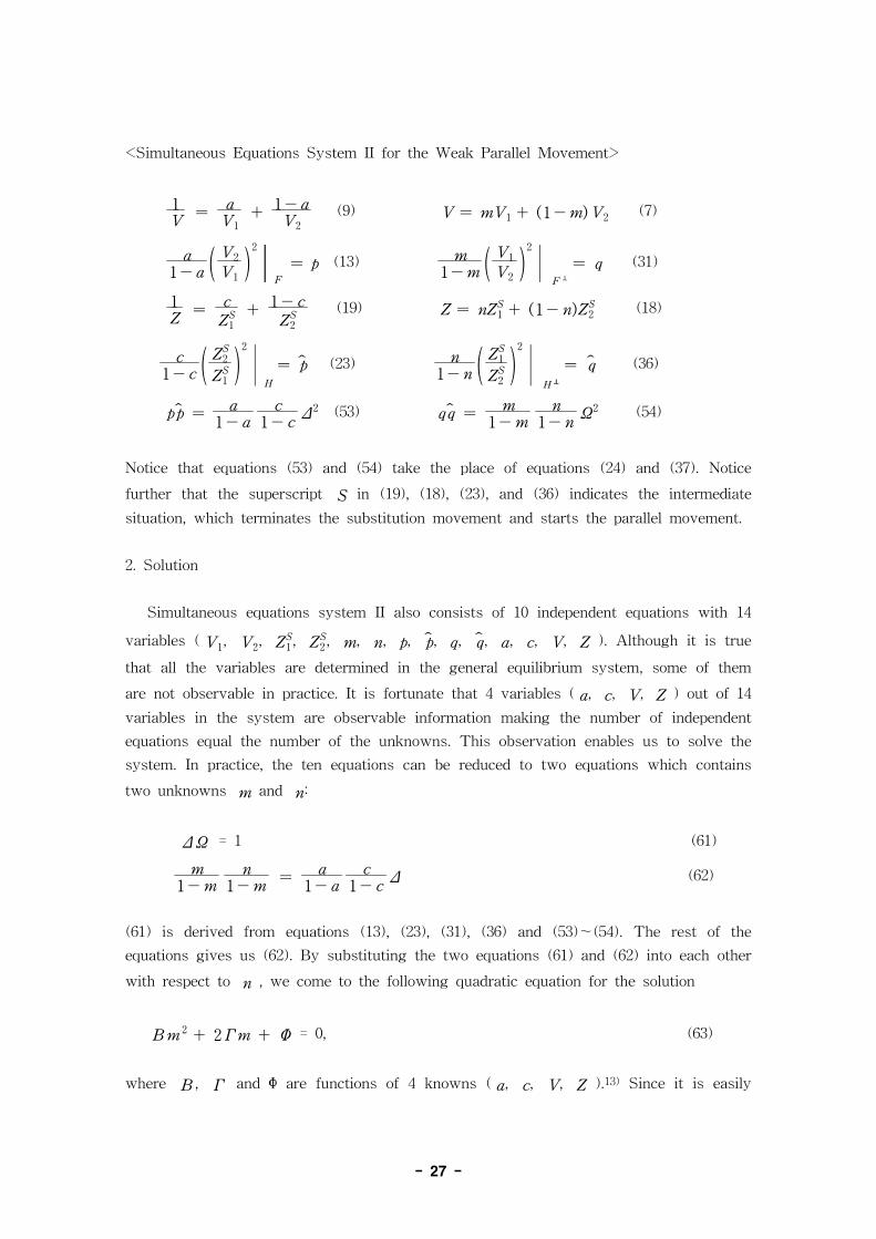
- 27 -
<Simultaneous Equations System II for the Weak Parallel Movement>
1V=
aV 1+1-aV 2
(9) V = mV 1 + (1-m)V 2 (7)
a1-a (
V 2V 1 )
2
┃F
= p (13) m1-m (
V 1V 2 )
2
│F ꠍ
= q (31)
1Z=
c
ZS1
+1-c
ZS2
(19) Z = nZS1 + (1-n)ZS2 (18)
c1-c (
ZS2
ZS1 )2
│H
= p̂ (23) n1-n (
ZS1
ZS2 )2
│H ꠍ
= q̂ (36)
p p̂ =a1-a
c1-c
Δ2 (53) q q̂ =m1-m
n1-n
Ω2 (54)
Notice that equations (53) and (54) take the place of equations (24) and (37). Notice
further that the superscript S in (19), (18), (23), and (36) indicates the intermediate
situation, which terminates the substitution movement and starts the parallel movement.
2. Solution
Simultaneous equations system II also consists of 10 independent equations with 14
variables ( V 1, V 2, ZS1, ZS2 , m, n, p, p̂, q, q̂, a, c, V, Z ). Although it is true
that all the variables are determined in the general equilibrium system, some of them
are not observable in practice. It is fortunate that 4 variables ( a, c, V, Z ) out of 14
variables in the system are observable information making the number of independent
equations equal the number of the unknowns. This observation enables us to solve the
system. In practice, the ten equations can be reduced to two equations which contains
two unknowns m and n:
Δ Ω = 1 (61)
m1-m
n1-m
=a1-a
c1-c
Δ (62)
(61) is derived from equations (13), (23), (31), (36) and (53)~(54). The rest of the
equations gives us (62). By substituting the two equations (61) and (62) into each other
with respect to n , we come to the following quadratic equation for the solution
Βm 2 + 2 Γm + Φ = 0, (63)
where Β , Γ and Φ are functions of 4 knowns ( a, c, V, Z ).13) Since it is easily

- 28 -
verified without presentation of the proof that Γ 2- ΒΦ > 0, the quadratic equation
(63) has two real solutions. One of them satisfies the condition (8) such that 1 > m > 0
[The proof is omitted]. Thus, the 'true' solution of (63), the sectoral money ratio at the
final point F[p], is given by
m = M 1M │
F( p)
=( a1- a
c1- c
Δ )½
1+( a1- a
c1- c
Δ )½ - G (64)
where
G = ( a1- a
c1- c
Δ)½
[ ( 1-D ½)+ (D- VZ )½
]1-
a1- a
c1- c
Δ
(65)
D = 1-aa
1-cc
1Δ [12
Δ1+Δ (
VZ-1)(1+ a
1-ac1-c )]
2
+VZ (66)
The relationship between the money ratio m and the parameter ( a, c, V, Z ) are not
known a pri-o-ri.
Next, substituting (64) into (7) and using (9), we have the sectoral velocities at the
final point F[p] as follows:
V 1V │
F ( p )=
a [ 1 + ( a1-a
c1-c
Δ )½
]( 1-G ) [ a
1-ac1-c
Δ ]½
- G
(67)
V 2V │
F ( p )=
(1-a) [ 1 + ( a1-a
c1-c
Δ )½
]1+G [1+ ( a
1-ac1-c
Δ )½
] (68)
It is verified that V 1≠V 2 at the final point F[p] and V 1 > 0 and V 2 > 0. [The
proof is omitted]. The relationship between the sectoral velocity ( V 1, V 2 ) and the
parameter ( a, c, V, Z ) are not known a pri-o-ri. Finally, if we substitute (67)~(68)
into system II, ZS1≠ZS2 at the intermediate point H. [The proof is omitted]. The form
of (64) and (67)~(68) is not simple by the looks but simple with numbers in practice. If
it is not simple, the calculation for the sectoral velocity formula is tedious and time
consuming to do by hand. To be practical use in practice, these must be calculated
13) Β= (1- a1- a
c1- c
Δ)(1+Δ) , Φ=-( VZ +Δ)a1- a
c1- c
Δ ,
Γ=12 [
a1-a
c1- c (
VZ+Δ)-(1- a
1-ac1- c
Δ)+( VZ +a1-a
c1-c )]Δ

- 29 -
quickly and repeatedly. Accordingly, it is essential that the practitioners have computer
facilities available.14)
VII. Conclusions
This paper discusses the basic method behind the bifurcation process of
decomposition of the economy-wide velocity. This process can continue to any sub-level
of transactions in a straightforward manner. The importances of finding disaggregated
monies and their velocities should not be overlooked.
In practice, for example, we could think of an immediate application to a country's
annual series of real and financial transactions. Or one may find the decomposition
useful in analyzing the effect of the newly born euro money on each member country's
velocity after the European monetary union is established. Identifying regional or
industrial monies and their velocities would assist the monetary authorities to allocate
the limited amount of available credit more effectively. From the macroeconomic point of
14) As we have witnessed thus far, this system can solve the final point F[p], but cannot
solve the initial point J[po]. [The proof is omitted]. This is due to the decomposition of
the overall movement into the substitution effect from point J[p o ] to point H[ p̂ ] along
the same old indifference curve Z[c] and the parallel movement effect from point H[ p̂ ]
in the old indifference curve Z[c] to point F[p] in the new indifference curve V[a].
The second way of expressing the same overall movement is to define firstly the parallel
movement effect from point J[p o ] in the old indifference curve Z[c] to point X[ p̂̂ ] in
the new indifference curve V[a], and define secondly the substitution effect from point
X[ p̂̂ ] to point F[p] in the new indifference curve V[a]. This system can solve the
initial point J[p o ], but cannot solve the final point F[p]. However, the solution of the
initial point J[p o ] is inappropriate and hence the second way is ruled out because the
solution is a function of not only c and Z of the initial point J[p o ] but also a and V
of the final point F[p] which are not known at the initial point J[p o ]. That is, the
solution of the initial point J[p o ] in the second way of decomposition is forwarding. This
implies that the solution of the final point F[p] in the second way is forwarding as well.
This is the reason the final point F[p] cannot be solved in the second way. On the
contrary, the solution of the final point F[p] in the first way of decomposition is
backward and a function of its contemporary weight a and magnitude V, plus its
previous weight c and magnitude Z all of which are known at the final point, as we
saw in equation (67) and (68). By the same token, the solution of the initial point J[p o ]
in the second way is determined by not only its contemporary weight c and magnitude
Z but also its previous weight and magnitude, which are known but not included in the
simultaneous equation system in the above. This is the reason we take the backward
solution.

- 30 -
view, the knowledge of financial and real velocities over time would be critically
important in analyzing the episode like " the great velocity decline." The velocity series
for real income process would provide clues on the short-run and long-run effects of
monetary policy.
In theory, the decomposition of the transaction velocity of money presented in this
paper would provide the general method for the reverse case that any aggregate
measure is disaggregated into sub-level components with limited information. One could
apply the same method to the capital asset pricing model, among others, to calculate the
beta, a measure of risk and an weight given to the linear combination of different rates
of return. In general, the possibilities of potential application to any linear combination
seem unlimited.
References
Bain, K. and P.G.Howells(1991), "The Income and Transactions Velocities of Money,"
Review of Social Economy, 1991, 383-395.
Bank for International Settlements(1996), Statistics on Payment Systems in the Group of
Ten Countries, Basle: Bank for International Settlements, 1996.
________________________________(1999), Central Bank Survey of Foreign Exchange and
Derivative Market Activity, Basle: Bank for International Settlements, 1999.
Boeschoten, W.J. and M.M.G. Fase (1984), The Volume of Payments and the Informal
Economy in the Netherlands 1965-1982. Monetary Monographs no. 1, Amsterdam: de
Netherlands Bank, and Dordrecht: Nijhoff.
Bordo, M.D. (1987), The Long-run Behavior of the Velocity of Circulation, Cambridge :
Cambridge University Press, 1987.
____________ (1989), "Equation of Exchange," in J. Eatwell et. al. (eds.), Money, the new
Palgrave series, New York: Norton, 151-156.
Cramer, J.S. and G.M.Reekers (1976), "Money Demand by Sector," Journal of Monetary
Economics 2(1), January 99-112.
___________. (1981), "The Work Money Does - The Transaction Velocity of Circulation
of Money in the Netherlands, 1950-1978," European Economic Review, 1981, 307-26,
___________, (1981), "The Volume of Transactions and Payments in the United Kingdom,
1968-1977," Oxford Economic Papers 33(2), July, 234-55.
___________, (1989), "Velocity of Circulation," in J. Eatwell et. al. (eds.), Money, the new
Palgrave series, New York: Norton, 328-332.
Davidson, P. (1997), "Are Grains of Sand in the Wheels of International Finance
Sufficient to do the Job when Boulders are often Required ?" Economic Journal 107,
671-686.
des Essars, P. (1895), "La vitesse de la circulation de la monnaie," Journal de la Societe
de Statistique de Paris, vol. 36, 143-26.

- 31 -
Eichengreen and Wyplosz (1993), "The Unstable EMS," Brookings Papers on Economic
Activity, 51-143.
Fisher, I. (1909), "A Practical Method for Estimating the Velocity of Circulation of
Money," Journal of the Royal Statistical Society 72, September, 604-11.
_________ (1911), The Purchasing Power of Money, New York: Macmillan
Friedman, M.(1987), "Quantity Theory of Money," in J. Eatwell et. al. (eds.), The New
Palgrave A Dictionary of Economics, vol. 4, London: Macmillan, 3-20.
Garvy, G. and M. R. Blyn, The Velocity of Money, New York: Federal Reserve Bank of
New York, 1969.
Howells, P.G., and I.B-F. Mariscal (1992), "An Explanation for the Recent Behavior of
Income and Transaction Velocities in the United Kingdom," Journal of Post
Keynesian Economy, 1992, 367-88.
Humphrey, T. M. (1993), "The Origins of Velocity Functions," Federal Reserve Bank of
Richmond Economic Quarterly, Fall 1993, 1-17.
Ireland, P. N. "Financial Evolution and the Long-Run Behavior of Velocity : New
Evidence from U.S. Regional Data," Federal Reserve Bank Richmond Economic
Review, vol. 77 (November / December 1991), pp.16-26.
Keynes, J.M. (1930), A Treatise on Money, London: Macmillan
Keynes, J.M.(1936), The General Theory of Interest, Employment and Money, London:
Macmillan.
Laurent, R.D. (1970), Currency Transfers by Denomination, Ph.D Dissertation, University
of Chicago.
McGouldrick, P. F., "A Sectoral Analysis of Velocity," Federal Reserve Bulletin
(December 1962).
Miller, R.D.(1979), "The Dynamic Properties of a Two Region Model of the Regional
Impact of Monetary Policy in the United States," Journal of Economics and Business,
1979, 90-102.
Petty, W.(1662), Treatise of Taxes and Contributions, 1662. In Charles Hull, ed., The
Economic Writings of Sir William Petty, I, Cambridge, 1899, reprinted, New York:
A. M. Kelly, 1964.
Samuelson, P.A. (1965), Foundations of Economic Analysis, New York: Atheneum.
Selden, R. T., "The Postwar Rise in the Velocity of Money : A Sectoral Analysis, "
Journal of Finance (December 1961).
Snyder, C.(1924), "New Measures in the Equation of Exchange," American Economic
Review.
_________. (1934), "On the Statistical Relation of Trade, Credit, and Prices," Revue de
l'Institut International de Statistique 2, October, 278-91.
Tobin, J.(1984), "On the Efficiency of the Financial System," Lloyds Bank Review (July
1984), 1-15.
Weinberg, J.A.(1994), "Selling Federal Reserve Payment Services: One Price Fits All ?"
Federal Reserve Bank of Richmond Economic Quarterly (Fall 1994), 1-24.

- 32 -
Figure 1. The Decomposition of the Transactions Velocity in the Fisherian Space
V 2, Z 2 45°
` Z[m 0]
▮ X[ p̂̂ ]
J[p 0]
E
H[ p̂] W G
E F[p] (1-a)V Z[c] (1-c)Z OV V[a]
OZ
Z[n] V[m]
O cZ aV V 1, Z 1
Figure 2. The Decomposition of the Transactions Time in the Marshallian Space
k 2,K 2
45°
E
ꠍ
F ꠍ[q] w
g ▮ Hꠍ[ q̂]
▮ K[n] (1-n)K E
ꠍ OK J
ꠍ[q 0 ] K[m 0]
(1-m)k Ok k[m] K[c] k[a] O k 1,K 1 mk nK

- 33 -
Appendix on Alternative Proof of Theorem 3 [ Equation (53) and (54) ]
This appendix may be cut off due to its excessive length after the verification of the
same result as the one given by the proof in the main text.
Step 1. Our primary concern is to establish the relationship between the slope p of
point F[p] and the slope p̂ of point H[ p̂ ], which is described by equation (53) in the
Fisherian space. This relationship, as the exact copy of the Marshallian space, should be
reflected by equation (54) between the slope q of point Fꠍ[q] and the slope q̂ of
point H ꠍ[ q̂ ]. In the Fisherian space of <Figure 1>, we take point G=(G,G ) in the
place where the straight line FH, connecting point F[p] and point H[ p̂ ], meets the 45
degree line. Then, the slope of line FH is defined by
slope of FH =V 2-Z 2V 1-Z 1
=V 2-G
V 1-G or
V 2-Z 2V 1-Z 1
=Z 2-G
Z 1-G (A-1)
At the same time in the Marshallian space of <Figure 2>, we take point w=(w,w )
in the place where the straight line F ꠍH ꠍ, connecting point F ꠍ[q] and point H ꠍ[ q̂ ],
meets the 45 degree line. Then, the slope of line FꠍH
ꠍ is defined by
slope of F ꠍH ꠍ=
k 2-K 2k 1-K 1
=k 2-w
k 1-w or
k 2-K 2k 1-K 1
=K 2-w
K 1-w (A-2)
Step 2. Theorem 2 implies implicitly that it is possible to meet simultaneously the
double condition p= p̂ and q= q̂ in both spaces if one of the two solutions is allowed
to be trivial on the 45 degree line, which is solution (50) or (51). To achieve this trivial
solution, we add in imagination an instrumental indifference curve G[cG ] which cuts
through the 45 degree line at point G=(G,G ) in the Fisherian space of <Figure 1>:
1G=cGG 1+1-cGG 2
(A-3)
The slope of the tangent line to at a point of this instrumental indifference curve
G[cG ] is defined as p̂ G , Then, we have from the law of equal marginal velocities
p̂ G=cG1-cG (
G 2G 1 )
2
(A-4)

- 34 -
In the Marshallian space of <Figure 2>, we also add in imagination the counterpart
indifference curve g[ng ] to this Fisherian instrumental indifference curve G[cG ] ;
1g=ngg 1+1-ngg 2
(A-5)
where gG=1, g 1G 1=1, g 2G 2=1. The slope of the tangent line to a point of this
indifference curve g[ng ] is defined as q̂ g. Then, we have the law of equal marginal
transactions time
q̂ g=ng1-ng (
g 2g 1 )
2
(A-6)
The above functions form the simultaneous equations system for the relationship
between a point of the indifference curve G[cG ] and point H[ p̂ ]= (Z 1,Z 2 ) of the
indifference curve Z[c] in the Fisherian space and the relationship between a point of
the indifference curve g[ng ] and point Hꠍ[ q̂ ] of the indifference curve K[n] in the
Marshallian space as follows:
1Z=cZ 1+1-cZ 2
Z=n Z 1+(1-n )Z 2
p̂=c1-c (
Z 2Z 1 )
2
q̂=n1-n (
Z 1Z 2 )
2
1G=cGG 1+1-cGG 2
G=ngG 1+(1-ng )G 2
p̂ G=cG1-cG (
G 2G 1 )
2
q̂ g= ng1-ng (
G 1G 2 )
2
To investigate the co-presence of the strong parallel movement effects in both spaces,
we add the following parallel movement conditions
p̂= p̂ G , q̂= q̂ g (A-7)
These conditions are equivalent to the conditions (49) in the main text. The solution to
this system, according to Theorem 2, is the following :
G 1=G 2 =G g 1=g 2 =g (A-8)

- 35 -
Z 1= c [ 1+( 1- cc1
p̂ )½
]Z K 1= n [ 1+( 1-nn1
q̂ )½
]K (A-9)
Z 2= (1- c) [1+( c1- c
p̂)½
]Z K 2= (1-n) [1+( n1-n
q̂)½
]K (A-10)
The solution is the specific form of the solution (51) in the main text [see footnote 10].
Step 3. The same step is taken for the indifference curve V[a] in the Fisherian space
of <Figure 1>. We take another point W =(W ,W ) between lower point E and point
G on the 45 degree line where another instrumental indifference curve W [aW ] passes
through ;
1W=aWW 1+1-aWW 2
(A-11)
The slope of the tangent line to a point of this indifference curve W [aW ] is defined as
pW . This leads us to the law of equal marginal velocities
pW =aW1-aW (
W 2W 1 )
2
(A-12)
Now, we further imagine the counterpart indifference curve w[mw] in the Marshallian
space to the Fisherian indifference curve W [aW ] as follows:
1w=mww 1+1-mww 2
(A-13)
where wW=1, w 1W 1=1, w 2W 2=1. The slope of the tangent line to a point of this
indifference curve w[mw ] is defined as qw . This leads us to the law of equal
marginal transactions time
qw=mw1-mw (
w 1w 2 )
2
(A-14)
The above equations form the simultaneous equations system for the relationship
between point F[p]= (V 1,V 2 ) of the indifference curve V[a] and a point of the
indifference curve W [aW ] in the Fisherian space and the relationship between point
F-1[q] of the indifference curve V[m] and a point of the indifference curve W [mw ]

- 36 -
in the Marshallian space as follows:
1V=aV 1+1-aV 2
V=mV 1+(1-m )V 2
p=a1-a (
V 2V 1 )
2
q= m1-m (
V 1V 2 )
2
1W=aWW 1+1-aWW 2
W=mwW 1+(1-mw )W 2
pW=aW1-aW (
W 2W 1 )
2
qw= mw1-mw (
W 1W 2 )
2
To investigate the co-existence of the strong parallel movement effects in both spaces,
we add the following conditions
p= pW , q= qw (A-15)
These conditions are also equivalent to the conditions (49) in the main text. The
solution to this system, according Theorem 2, is
W 1=W 2 =W w 1=w 2 =w (A-16)
V 1= a [1+( 1-aa1p )
½
]V k 1= m [1+( 1-mm1q )
½
]k (A-17)
V 2= (1-a) [ 1+( a1-a
p)½
]V k 2= (1-m) [1+( m1-m
q)½
]Z (A-18)
The solution is the concrete form of solution (50) in the main text [see footnote 9].
Step 4. Now, let us transform Fisherian slope (A-1) of the straight line FH into the
Marshallian space. The result is
k 2-g
k 1-g=(K 1K 2 )(
k 2-K 2k 1-K 1 ) or
K 2-g
K 1-g=(k 1k 2 )(
k 2-K 2k 1-K 1 ) (A-19)
These are different from slope (A-2), which stands for the slope of the straight line
F ꠍH ꠍ in the Marshallian space. Since K 1 >K 2, the first slope of (A-19) between point
F ꠍ[q ] and point g is greater than the first slope of (A-2) between point F ꠍ[q] and
point H ꠍ[ q̂ ]. Since k 1 < k 2, the second slope of (A-19) between point H ꠍ[ q̂ ] and g is
smaller than the second slope of (A-2) between Hꠍ[ q̂ ] and point F ꠍ[q]. This implies
that the Fisherian straight line FH becomes kinky line F ꠍgH ꠍ in the Marshallian

- 37 -
space with aid of the transformation and point g is different from point w. Point g
plays a pivot role in transformation.
By the same token, let us further transform the Marshallian slope (A-2) of the
straight line F ꠍH ꠍ into the Fisherian space to become
V 2-W
V 1-W=(Z 1Z 2 )(
V 2-Z 2V 1-Z 1 ) or
Z 2-W
Z 1-W=(V 1V 2 )(
V 2-Z 2V 1-Z 1 ) (A-20)
These are different from equation (A-1), which stands for the slope of the straight line
FH in the Fisherian space. Since Z 1 <Z 2, the first slope of (A-20) between point
F[p] and point W is smaller than the first slope of (A-1) between point F[p] and
point H[ p̂ ]. Since V 1 >V 2, the second slope of (A-20) between point H[ p̂ ] and point
W is greater than the second slope of (A-1) between point H[ p̂ ] and F[p]. This
implies that the Marshallian straight line FꠍH
ꠍ becomes kinky line FWH in the
Fisherian space through transformation and point W is different from point G. Point W
is a pivot.
The above analysis presents impossibility of the simultaneous straight lines in both
spaces. The straight line FH in the Fisherian space is transformed to become the
kinky line F ꠍgH ꠍ in the Marshallian space, while the straight line F ꠍH ꠍ in the
Marshallian space is transformed to become the kinky line FWH in the Fisherian
space. However, the Fisherian kinky line HGWF which kinked twice at W and G
becomes the exact image of the Marshallian kinky line HꠍgwF
ꠍ which kinked twice at
w and g.
The kinky line HGWF in the Fisherian space is represented by the following two
slopes:
V 2-W
V 1-W=(Z 1Z 2 )(
V 2-Z 2V 1-Z 1 ) ,
Z 2-G
Z 1-G=V 2-Z 2V 1-Z 1
(A-21)
The first one represents the slope of the line segment FW and the second one the
slope of the line segment HG. By the same way, the kinky line HꠍgwF
ꠍ in the
Marshallian space is represented by the following two slopes :
k 2-w
k 1-w=k 2-K 2k 1-K 1
, K 2-g
K 1-g=(k 1k 2 )(
k 2-K 2k 1-K 1 ) (A-22)
The first one represents the slope of the line segment Fꠍw and the second one the

- 38 -
slope of the line segment H ꠍg. One may verify that first slope of (A-22) is
transformed to become the first slope of (A-21) and the second slope of (A-22) is
transformed to become the second slope of (A-21).
Step 5. Equations (A-9), (A-10), (A-17), (A-18), and (A-21) in the Fisherian space
form the following simultaneous equations system for the kinky phenomenon :
V 1= a [1+( 1-aa1p )
½
]V Z 1= c [ 1+( 1- cc1
p̂ )½
]Z
V 2= (1-a) [ 1+( a1-a
p)½
]V Z 2= (1- c) [ 1+( c1- c
p̂)½
]Z
V 2-W
V 1-W=(Z 1Z 2 )(
V 2-Z 2V 1-Z 1 )
Z 2-G
Z 1-G=V 2-Z 2V 1-Z 1
Substituting the first four equations into the kinky slope of line segment FW yields
( p p̂ ) ½ =θ
aV- cZ(p ) ½+( a
1- ac1- c )
½
Δ (A-23)
where
θ= [ ( 1- a) ( a1- a )
½
- a( c1- c )
½
( pp̂ )½
]V
+[c ( a1- a )
½
-(1- c) ( c1- c )
½
( pp̂ )½
]Z-[ ( a1- a )
½
-( c1- c )
½
( pp̂ )½
]W
This establishes the kinky relationship between point F[p] and point H[ p̂ ] in the
Fisherian space.
The same method may be applied to the Marshallian space with the aid of the
simultaneous kinky line phenomenon (A-9), (A-10), (A-17), (A-18), and (A-22) in the
Marshallian space to form the following simultaneous equations system.
k 1= m [ 1+( 1-mm1q )
½
]k K 1= n [1+( 1-nn1
q̂ )½
]K
k 2= (1-m) [ 1+( m1-m
q)½
]k K 2= (1-n) [ 1+( n1-n
q̂)½
]K
K 2-g
K 1-g=(k 1k 2 )(
k 2-K 2k 1-K 1 )
k 2-w
k 1-w=k 2-K 2k 1-K 1
Substituting the first four equations into the kinky slope of line gHꠍ yields
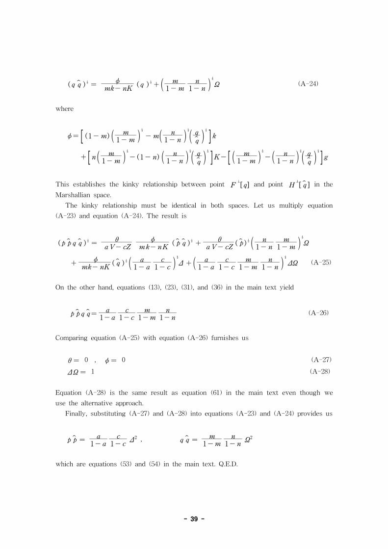
- 39 -
(q q̂ ) ½ =φ
mk- nK(q ) ½+( m
1-mn1- n )
½
Ω (A-24)
where
φ= [ (1-m ) ( m1-m )
½
-m ( n1- n )
½
( qq̂ )½
] k
+[n ( m1-m )
½
-(1-n) ( n1-n )
½
( qq̂ )½
]K-[ ( m1-m )
½
-( n1-n )
½
( qq̂ )½
]g
This establishes the kinky relationship between point F ꠍ[q] and point Hꠍ[ q̂ ] in the
Marshallian space.
The kinky relationship must be identical in both spaces. Let us multiply equation
(A-23) and equation (A-24). The result is
(p p̂ q q̂ ) ½ =θ
aV- cZφ
mk-nK( p̂ q̂ ) ½ +
θaV- cZ
( p̂ )½ ( n1-n
m1-m )
½
Ω
+φ
mk- nK( q̂ ) ½ ( a
1- ac1- c )
½
Δ +( a1- a
c1- c
m1-m
n1-n )
½
ΔΩ (A-25)
On the other hand, equations (13), (23), (31), and (36) in the main text yield
p p̂ q q̂=a1-a
c1-c
m1-m
n1-n
(A-26)
Comparing equation (A-25) with equation (A-26) furnishes us
θ = 0 , φ = 0 (A-27)
ΔΩ = 1 (A-28)
Equation (A-28) is the same result as equation (61) in the main text even though we
use the alternative approach.
Finally, substituting (A-27) and (A-28) into equations (A-23) and (A-24) provides us
p p̂ =a1-a
c1-c
Δ2 , q q̂ =m1-m
n1-n
Ω2
which are equations (53) and (54) in the main text. Q.E.D.