new updating criteria for conflict-based branching heuristics in dpll algorithms for satisfiability

Discrete Optimization 5 (2008) 569–583www.elsevier.com/locate/disopt

New updating criteria for conflict-based branching heuristics inDPLL algorithms for satisfiability

Renato Bruni∗, Andrea Santori

Universita di Perugia - D.I.E.I., Via G. Duranti, 93 - 06125 Perugia, Italy

Received 20 October 2004; received in revised form 12 October 2006; accepted 15 October 2006Available online 12 February 2008

Abstract

The paper is concerned with the computational evaluation and comparison of a new family of conflict-based branching heuristicsfor evolved DPLL Satisfiability solvers. Such a family of heuristics is based on the use of new scores updating criteria developedin order to overcome some of the typical unpleasant behaviors of DPLL search techniques. In particular, a score is associatedwith each literal. Whenever a conflict occurs, some scores are incremented with different values, depending on the character ofthe conflict. The branching variable is then selected by using the maximum among those scores. Several variants of this havebeen introduced into a state-of-the-art implementation of a DPLL SAT solver, obtaining several versions of the solver havingquite different behavior. Experiments on many benchmark series, both satisfiable and unsatisfiable, demonstrate advantages of theproposed heuristics.c© 2007 Elsevier B.V. All rights reserved.

Keywords: Branching rules; Conflict-based search frameworks; Satisfiability

1. Introduction

A propositional formula F in Conjunctive Normal Form (CNF) is a conjunction of clauses C j , each clause beinga disjunction of literals, each literal being either a positive (xi ) or a negative (¬xi ) propositional variable, withj ∈ {1, . . . , m}, i ∈ {1, . . . , n}. By denoting with I j the set of variables of C j , and with [¬] the possible presence of¬, this is

∧j=1...m

∨i∈I j

[¬] xi

.

The satisfiability problem (SAT) consists in determining whether there exists a truth assignment in {0, 1}(or equivalently in {False, True}) for the variables such that F evaluates to 1. Extensive references can be found in[6,14,23]. Many problems arising from different fields, such as artificial intelligence, logic circuit design and testing,cryptography, database systems, and software verification, are usually encoded as SAT. Moreover, SAT carries

∗ Corresponding author.E-mail addresses: [email protected] (R. Bruni), [email protected] (A. Santori).

1572-5286/$ - see front matter c© 2007 Elsevier B.V. All rights reserved.doi:10.1016/j.disopt.2006.10.012

http://www.elsevier.com/locate/disopt

mailto:[email protected]

mailto:[email protected]

http://dx.doi.org/10.1016/j.disopt.2006.10.012

570 R. Bruni, A. Santori / Discrete Optimization 5 (2008) 569–583

considerable theoretical interest as the original NP-complete problem [7,11]. From the practical point of view, thisimplies that many instances require an exponentially bounded computational time for their solution, but also thatinvesting in the cleverness of the solution algorithm can result in very large savings in such computational times.The above has motivated a wide stream of research in practically efficient SAT solvers. As a consequence, manyalgorithms for solving the SAT problem have been proposed, based on different techniques (see for instance [8,9,12,14,17]). Computational improvements in this field are impressive (see, e.g., [17,22]). However, even if the sizeand difficulty of the instances which can be solved are greatly increasing, also the size and difficulty of the instanceswhich are needed to be solved are greatly increasing (just to give an example, think about the case of microprocessorverification).

A solution method is said to be complete if it guarantees (given enough time) finding a solution if one exists, orproves lack of a solution otherwise. Incomplete, or stochastic, methods, on the contrary, cannot guarantee finding thesolution, although they may scale better than complete methods, mainly on large satisfiable problems. Most of thebest complete solvers are based on so-called Davis–Putnam–Logemann–Loveland (DPLL) enumeration techniques.From the initial relatively simple DPLL backtracking algorithm described in [8], SAT solvers have evolved byexperimenting with several more sophisticated branching and backtracking frameworks, and eventually incorporatingthe best ones. Noteworthy examples of this have been non-chronological backtracking and conflict-driven clauselearning [1,19]. These techniques greatly improve the efficiency of DPLL algorithms, especially for structured SATinstances. Subsequently, a further generation of solvers paying special attention to implementation aspects appeared:SATO [25], Chaff [21], BerkMin [13] and several others, sometimes referred to as chaff-like solvers [17]. Such solversnowadays appear to be the most competitive in solving real-world satisfiability problems.

As a matter of fact, a relevant influence on computational behavior is given by the branching rule, or branchingheuristic, that is how to chose, at each branching, the next variable assignment. Different branching heuristics forthe same basic algorithm may result in completely different computational results [20,24]. Early branching heuristics(e.g., Bohm [4], MOM [14], Jeroslow–Wang [16]) have often been viewed as greedy trials of simplifying as muchas possible the current subproblem, for instance by satisfying the most clauses. Such heuristics are based on a prioristatistics on the instance, and have a certain effectiveness in the case of randomly generated problems. However, theyusually cannot capture hidden problem structure, and real world problems typically are quite well structured. In orderto tackle such problems, heuristics based on the history of the search, and in particular on the history of conflicts, havebeen proposed. Examples are the VSIDS heuristic of Chaff [21], the adaptive branching rule of ACS [2], BerkMindecision-making strategy [13], and the dynamic selection of branching rules [15]. Conflict-based heuristics generallykeep dynamically updated scores associated with variables. A central issue is then the policy for updating such scores.Recent studies on evolved scores updating techniques are also reported in [5] and in a preliminary version of presentpaper [3].

We report here a computational study of new scores updating criteria for conflict-based branching heuristics. Suchcriteria have been developed in order to overcome a part of the typical time-wasting behaviors of DPLL searchtechniques, as described in Section 2. In particular, a score is associated with each literal. Whenever a conflict occurs,some scores are incremented with different values, depending on the character of the conflict, as illustrated in detail inSection 3. The branching variable is then selected by using the maximum among those scores. Therefore, a new familyof conflict-based branching heuristics for evolved DPLL Satisfiability solvers, called the Reverse Assignment Sequence(RAS), is obtained. Such heuristics have been introduced into a state-of-the-art implementation of a DPLL SAT solver,obtaining several versions of the solver having quite different behaviors, as described in Section 4. Experiments onmany benchmark series, both satisfiable and unsatisfiable, show that the proposed branching heuristics are often ableto improve solution times. Moreover, notwithstanding the fact that the introduced counter updating requires somecomputational overhead for its operations, total solution times on each series are always in favor of one of the newversions of the solver.

2. Motivations and aims of new updating criteria

For a DPLL-based algorithm, the search evolution is often represented as the exploration of a search tree, whereeach node subproblem is obtained by assigning a variable. The fact that SAT is an NP-complete problem impliesthat, for satisfiable instances, if one could choose at every node subproblem the correct truth assignment, that is thecorrect branch in the search tree, a satisfying solution would be obtained in a polynomial number of assignments [11].

R. Bruni, A. Santori / Discrete Optimization 5 (2008) 569–583 571

Unfortunately, unless P = NP, it seems unlikely that some practical algorithm doing this in polynomial time mayin general exist. Moreover, the problem of choosing at every node such an assignment for DPLL algorithms hasbeen proven to be NP-hard as well as coNP-hard [18]. Therefore, the (heuristic) policy governing the choice ofthe variable assignments is generally called the branching heuristic. Different branching heuristics may producedrastically different sized search trees for the same basic algorithm.

Conflict-based branching heuristics generally keep, for each variable xi , a counter, or score si , or sometimes twocounters, for the two possible truth assignments, or phases, of xi . Score si is incremented when xi is somehow involvedin a conflict, i.e., an empty clause is derived by current truth assignments. Branching variables are selected accordingto the values of such scores. Counters are often periodically proportionally reduced, both to avoid overflow problemsand to give to the earlier history of the search progressively less importance than the recent history. For instance, thezChaff [21] heuristic (called VSIDS for Variable State Independent Decaying Sum) uses for each variable two scoresinitialized to the number of occurrences of each literal in the instance. Whenever a new clause is learned, the counterof each of its literals is incremented by 1. The variable assignment corresponds to the literal having a maximum score.Also the adaptive branching heuristic of ACS [2] uses a score for each clause, since it operates with a clause-basedbranching tree. The score of each clause is incremented by a penalty pv each time an assignment aimed at satisfyingthat clause is made, and by another penalty p f each time that that clause causes a conflict. The variable assignmentis selected among literals contained in the unsatisfied clause having the maximum score. The BerkMin [13] heuristicuses one score for each variable. Whenever a conflict occurs, the scores of all variables contained in the clauses thatare responsible for the conflict are increased by 1. The variable assignment corresponds to the literal whose variablehas a maximum score among those contained in the last learned clause that is unresolved.

Conflict-based branching heuristics have the advantages of requiring low computational overhead and of beingoften able to detect the hidden structure of a problem. They therefore generally produce good results on large real-world instances. The motivations of this can be explained by noticing that such heuristics try to avoid, or at least topostpone, the exploration of some regions of the search space which are likely to produce an unpleasant behavior ofthe DPLL search algorithm.

We therefore try to follow along this line and develop more evolved techniques for altogether avoiding otherunpleasant phases of a DPLL search algorithm. There are in fact a number of situations that may denote that thesearch is passing through an unpromising and time-wasting phase. Note that the simple occurrence of such situationscannot guarantee that the search is exploring a useless region of the search space. Therefore, such phases cannotbe just forbidden or the search would become incomplete. Our aim is to avoid them, or at least postpone them, inorder to tackle them only when no better option is available. We propose, in particular, techniques for avoiding theunpleasant search phases denoted by the three situations described below, and also illustrated in Fig. 1. In the followingdescription, let the h-th level of the search tree be the set of nodes of the search tree having the same search tree depthh. We will speak intuitively of first levels, i.e., the nearest ones to the root, and of low levels, i.e., the most distant onesfrom the root.

(i) A first situation denoting an unpleasant phase is having many backtracks at the low levels of the search tree (Fig. 1part (i)). If indeed backtracks could be moved all at the very first levels of the search tree, either unsatisfiabilitywould be detected much earlier, or a satisfiable solution would be reached within a very limited number of uselessvariable assignments.

(ii) A second situation (Fig. 1 part (ii)) denoting an unpleasant phase is the repetition, in different branches of thesearch tree, of the same sequence of variable assignments leading to a conflict (e.g., . . . xi = vi , x j = v j , xk =

vk, xl = vl ). Conflict clause learning can only avoid, each time, the repetition of the last assignment of such asequence, but, without some adaptive heuristic, it does not prevent the search from moving again in the samedirection (e.g., . . . xi = vi , x j = v j , xk = vk). Although this search phase cannot be forbidden without makingthe search incomplete, it would be preferable to avoid it as far as it is possible.

(iii) Finally, it may often happen that some of the variables of an instance are related in such a way that, for largeportions of the branching tree, a conflict is always obtained at about the same decision level and due to a smallset of variables (Fig. 1 part (iii)). Such a phase is clearly time-wasting and should be avoided, even if, again, itcannot be forbidden.

The above three aims can be pursued by using the scores updating mechanism. Since in fact the branching decisionis taken on the basis of the maximum among such scores, by incrementing them in a suitable way we would be able to


Fig. 1. Representation of the described unpleasant search situations for a DPLL algorithm. Nodes corresponding to subproblems where an emptyclause is derived, and hence backtrack is performed, are represented in black. Search trees are represented in such a way that their explorationchronologically proceeds from right to left.

guide the search in order to avoid, but not forbid, the above phases. Note that such a list of situations denoting phasesthat should be avoided during the search, but which cannot be forbidden without making the search incomplete, couldalso be enriched, still remaining in the proposed algorithmic framework.

3. The proposed updating criteria

For each variable xi , i ∈ {1, . . . , n}, we use two counters, or scores, s0i and s1

i for the two possible phases of xi .Counters are therefore associated with the two possible literals v0(xi ) = ¬xi and v1(xi ) = xi . When branching isneeded, we assign, as usual, variable xi at value v ∈ {0, 1} by choosing the maximum score, as follows:

xi = v such that svi = max{s0

1 , s11 , . . . , s0

n , s1n}.

Similarly to other conflict-based heuristics, scores are initialized to the number of occurrences of each literal inthe instance, and periodically proportionally reduced. The main issue clearly is how scores {s0

1 , s11 , . . . , s0

n , s1n} are

incremented.In order to pursue the above point (i), we try to assign at first the more difficult variables, in the sense of the more

constrained ones. This is because, when assigning them in the upper levels of the search tree, we should either discoverunsatisfiability earlier or we should remain with only easy variables to assign in the lower levels of the search tree, andtherefore little backtrack should be needed there. Whenever a new learned clause Cl = {v(xl1), . . . , v(xlh)} is addedto the clause set by the effect of a conflict, what we have actually discovered is that variables {xl1, . . . , xlh} containedin Cl are a bit more constrained than other variables. In fact, Cl represents just such a constraint made explicit, that isalready implied by the original clauses. Therefore, we increment the scores of those literals by a penalty for learningpl , as follows:

svi ← sv

i + pl , ∀v(xi ) ∈ Cl

(where a ← a + b means that new value of a is obtained by adding b to its old value). The effect can also be viewedas trying to satisfy Cl . Note that, so far, this is also zChaff’s policy.

Moreover, in order to pursue the above point (ii), we try to reverse every sequence of assignments which leads toa conflict. Whenever a sequence of assignments produces an empty clause, this sequence is at risk of being repeated


again in the search tree, leading again to the same conflict. The use of learned clauses, together with the incrementof the scores of their literals, can only partially solve the problem. We therefore try to satisfy the failed clauseC f = {v(x f 1), . . . , v(x f k)} (the clause which has become empty) by incrementing the scores of its literals by apenalty for failure p f , as follows:

svi ← sv

i + p f , ∀v(xi ) ∈ C f .

After doing so, the subsequent assignments would be different, thus preventing the repetition of the above conflictingsequences of assignments. However, since increasing scores has a cost, and moreover implies an even higher costfor reordering the scores in order to choose the higher value, we also consider the possibility of applying somesimplifications to the above algorithm. In fact, adding p f to only one of the counters corresponding to the literalsof the failed clause C f , and in particular to the last assigned literal except the conflicting literal, decreases thecomputational overhead while maintaining most of the positive features. Several other alternatives were tested, but theabove proposed one appears more stable, in the sense of producing good results on different types of problems.

Finally, in order to pursue the above point (iii), we would like to avoid frequent backtracks due to the sameconflicting literal v(x f ) at the same decision level d . We therefore keep in memory the set of the last c conflict literalsand their corresponding levels, obtaining the set of couples M = {(v(x f 1), dq1), . . . , (v(x f c), dqc)}. Whenever anew conflict occurs due to literal v(x f ) at decision level dq , if the couple (v(x f ), dq) is already contained in M , weincrement the score of the direct conflicting literal by a penalty pd , and the score of the negation of the conflictingliteral by a penalty pn , as follows:{

svf ← sv

f + pd

s¬vf ← s¬v

f + pnif

{v(x f ) conflicts at level dqand already (v(x f ), dq) ∈ M.

There are in fact reasons for increasing the score of the conflicting literal v(x f ), and also reasons for increasing thescore of the negation of the conflicting literal ¬v(x f ). This is because, in the absence of further information, it shouldbe convenient to try to assign such a variable at an upper decision level, and, moreover, both its values may turnout to be useful since they both were “needed”. Since, however, increasing the two counters has a relatively highcomputational cost, we also consider the possibility of increasing only the counter of the conflicting literal v(x f ). Wewill briefly refer to the above operation as “frequent conflicting literals detection”.

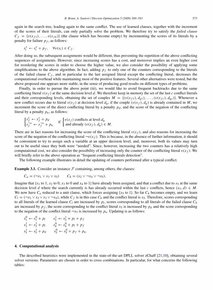
The following example illustrates in detail the updating of counters performed after a typical conflict.

Example 3.1. Consider an instance F containing, among others, the clauses:

Ca = (¬x1 ∨ x3 ∨ x5) Cb = (x2 ∨ ¬x4 ∨ ¬x5).

Imagine that {x1 to 1, x2 to 0, x3 to 0 and x4 to 1} have already been assigned, and that a conflict due to x5 at the samedecision level d where the search currently is has already occurred within the last c conflicts, hence (x5, d) ∈ M .We now have Ca reduced to a unit clause, which forces assigning {x5 to 1}. So far Cb becomes empty, and we learnCl = (¬x1 ∨ x2 ∨ x3 ∨¬x4), while C f is in this case Cb and the conflict literal is x5. Therefore, scores correspondingto all literals of the learned clause Cl are increased by pl , scores corresponding to all literals of the failed clause Cbare increased by p f , the score corresponding to the conflict literal x5 is increased by pd and the score correspondingto the negation of the conflict literal ¬x5 is increased by pn . Updating is as follows:

s01 ← s0

1 + pl s12 ← s1

2 + pl + p f

s13 ← s1

3 + pl s04 ← s0

4 + pl + p f

s15 ← s1

5 + pd s05 ← s0

5 + p f + pn .

4. Computational analysis

The described heuristics were implemented in the state-of-the-art DPLL solver zChaff [21,10], obtaining severalsolver versions. Parameters are chosen in order to cross combinations. In particular, for what concerns the followingtables:


Table 1Comparison on bounded model checking problems

Barrel Sol zChaff zCh1 zCh2 brChaff brCh1 brCh2 bChaff bCh1 bCh2

barrel2 U 0.01 0.00 0.00 0.00 0.00 0.01 0.00 0.00 0.013 3 3 5 5 5 5 5 5

barrel3 U 0.02 0.01 0.02 0.02 0.02 0.02 0.02 0.02 0.02154 127 101 119 119 119 192 152 228

barrel4 U 0.08 0.07 0.09 0.07 0.07 0.07 0.07 0.07 0.09197 197 197 182 182 182 368 368 368

barrel5 U 3.60 3.05 2.78 2.43 2.34 2.12 1.55 1.55 1.8611248 10832 9882 9083 9826 10596 8172 7860 7354

barrel6 U 18.60 14.91 13.32 11.74 13.62 12.43 9.70 11.39 10.8538816 34104 35280 31381 36311 32159 24727 29779 27057

barrel7 U 35.45 51.89 26.03 27.15 25.32 32.63 16.93 14.67 14.9054429 84568 57035 49911 54894 57721 46357 47706 47433

barrel8 U 227.03 189.79 127.08 118.54 164.93 122.45 74.81 66.15 80.40180853 199608 143429 149886 174569 124932 122492 136210 128030

barrel9 U 152.40 167.04 133.79 134.11 130.56 126.79 98.95 88.87 103.51417906 438875 368223 347597 365419 342494 282883 255763 282827

Total 437.19 426.76 303.11 294.08 336.87 296.52 202.04 182.73 211.62703606 768314 614150 588164 641325 568208 485196 477843 493302

• ‘zChaff’ is the original version of zChaff 2004 [10];• ‘zCh1’ is the version incrementing all literals of learned clauses using pl = 1 and frequent conflicting literals (not

their negations) using c = 2 and pd = 2;• ‘zCh2’ is the version incrementing all literals of learned clauses using pl = 1 and frequent conflicting literals and

their negations using c = 2, pd = 2 and pn = 2;• ‘brChaff’ is the version incrementing all literals of learned clauses using pl = 1 and the last literal of failed clauses

except the conflicting literal using p f = 2;• ‘brCh1’ is the same as ‘brChaff’ but also incrementing frequent conflicting literals using c = 2 and pd = 2;• ‘brCh2’ is the same as ‘brChaff’ but also incrementing frequent conflicting literals and their negations using c = 2,

pd = 2 and pn = 2;• ‘bChaff’ is the version incrementing all literals of learned clauses using pl = 1 and all literals of failed clauses

using p f = 2;• ‘bCh1’ is the same as ‘bChaff’ but also incrementing frequent conflicting literals using c = 2 and pd = 2;• ‘bCh2’ is the same as ‘bChaff’ but also incrementing frequent conflicting literals and their negations using c = 2,

pd = 2 and pn = 2.

Note that zChaff 2004 may also use, for a limited number of times, other branching heuristics in addition to theclassical VSIDS one. Our branching heuristics substituted completely the VSIDS one and only that one. Experimentsare conducted on a 2.5 GHz Intel Celeron PC with 512 MB RAM and using the MS VC++ compiler. Note also thatsome libraries may be different, using other compilers, therefore results may vary (we experienced this) but maintainabout the same average results on each series.

We report, in the first line of each entry of the tables, running times in CPU seconds. Time limit was set at 3600 s(1 h), when exceeded we report “–”. Total solution times are obtained by counting each time-out as 3600 s, exceptfor problems not solved by any solver (global time-outs), which are not counted in the totals. Since the total forsolvers incurring in non-global time-outs is actually a lower bound, we denote this by writing a > before the value.We report in bold face the best total time. We also report, in the second line of each entry of the tables, the numberof decisions, that is how many times the solver needs to select a variable and to assign it. Assignments which arejust forced consequences of such decisions (e.g., unit propagation) are not counted as decisions themselves. The totalnumber of decisions is obtained by counting each time-out as the maximum among the numbers of decisions made by


Table 2Comparison of data encryption problems

Des-encryption Sol zChaff zCh1 zCh2 brChaff brCh1 brCh2 bChaff bCh1 bCh2

cnf-r3-b1-k1.1 S 7.40 13.01 4.68 11.30 8.48 7.79 11.32 10.86 6.6128871 41410 21088 40471 28927 24138 35820 29596 23334

cnf-r3-b1-k1.2 S 4.34 9.01 4.05 16.49 6.06 20.10 4.26 16.42 13.8910755 25464 9449 29682 14819 46061 10287 40170 36021

cnf-r3-b2-k1.1 S 0.92 0.74 0.77 0.50 0.76 0.75 1.16 0.84 0.721328 862 1299 638 1236 899 1465 1042 994

cnf-r3-b2-k1.2 S 2.05 2.17 2.67 1.75 1.04 2.14 3.97 1.77 1.481243 2147 2034 1317 656 1378 3223 1240 915

cnf-r3-b3-k1.1 S 1.17 0.57 0.70 1.35 1.25 1.82 1.00 1.35 1.101129 577 890 1196 1217 1531 741 1063 1016

cnf-r3-b3-k1.2 S 1.77 2.03 1.91 2.18 2.33 1.63 1.05 2.04 1.76538 567 818 890 798 447 302 650 518

cnf-r3-b4-k1.1 S 0.91 1.04 1.12 1.04 0.95 1.75 1.23 1.32 1.25497 607 513 706 415 1239 491 573 562

cnf-r3-b4-k1.2 S 2.66 2.04 1.86 1.66 2.05 3.03 1.85 2.03 2.66640 421 557 242 477 631 341 326 675

cnf-r4-b1-k1.1/.2 – – – – – – – – – –– – – – – – – – –

cnf-r4-b2-k1.1 S – 1010.48 – 1270.94 3348.77 – 1610.48 – –– 2625565 – 2901880 5340918 – 3682226 – –

cnf-r4-b2-k1.2 S – – – 1026.18 2174.86 – 2095.12 – 1656.77– – – 2221151 4008092 – 3332414 – 2894610

cnf-r4-b3-k1.1 S 705.20 1314.44 – 1482.11 2611.29 – 667.92 1556.71 1150.481768757 2292924 – 2445872 3967580 – 1348190 3401421 2217073

cnf-r4-b3-k1.2 S 647.39 – 1551.82 558.12 – – 2067.51 693.69 252.23981196 – 2390076 1107932 – – 3169485 1053167 451757

cnf-r4-b4-k1.1 S 422.61 1361.78 2624.32 767.18 1663.30 1060.80 1106.74 1348.00 1041.60816444 2179918 3913826 1402128 2083653 1769687 1428725 1683870 1596734

cnf-r4-b4-k1.2 S 647.29 776.89 316.88 577.05 490.60 977.68 342.22 155.54 494.75657150 1003928 432733 716099 631319 1025376 465776 211683 655010

Total >9643.71 >11694.20 >15310.78 5717.85 >13911.74 >16477.49 7915.84 >10990.57 >8225.30>14950384 >18856226 >22796037 2193369 >21431025 >24195059 13479486 >17106637 >13319227

the other solvers which solved the time-outed problem, except for the problems which are not solved by any solver,which are not counted in the totals.

The considered benchmark series were provided by different authors to the SAT community and are now publiclyavailable. The majority of them were used as benchmarks in recent SAT Solver Competitions (see [22], both forbenchmark details and for past and probably future results of other solvers on them). Most of the considered series arereal-world problems, and are therefore structured, but we also considered one randomly generated series. The seriesare either all satisfiable, or all unsatisfiable, or mixed.

As a general remark, notwithstanding the fact that the introduced counter updating techniques require acomputational overhead for its operations compared to the original zChaff branching heuristic (especially for thedetection of frequent conflicting literals), computational times often decrease, proving the algorithmic effectivenessof the proposed updating criteria. Moreover, our experiments fully confirm that the branching rule has a very relevantinfluence on computational behavior: small modifications in it may cause completely different computational results.Versions incrementing literals of failed clauses tend to be good compromises between speed and stability. On the otherhand, versions incrementing frequent conflicting literals tend to be less stable: sometimes they are the fastest, but theyare often the slowest for easy instances due to their heavier computational load.


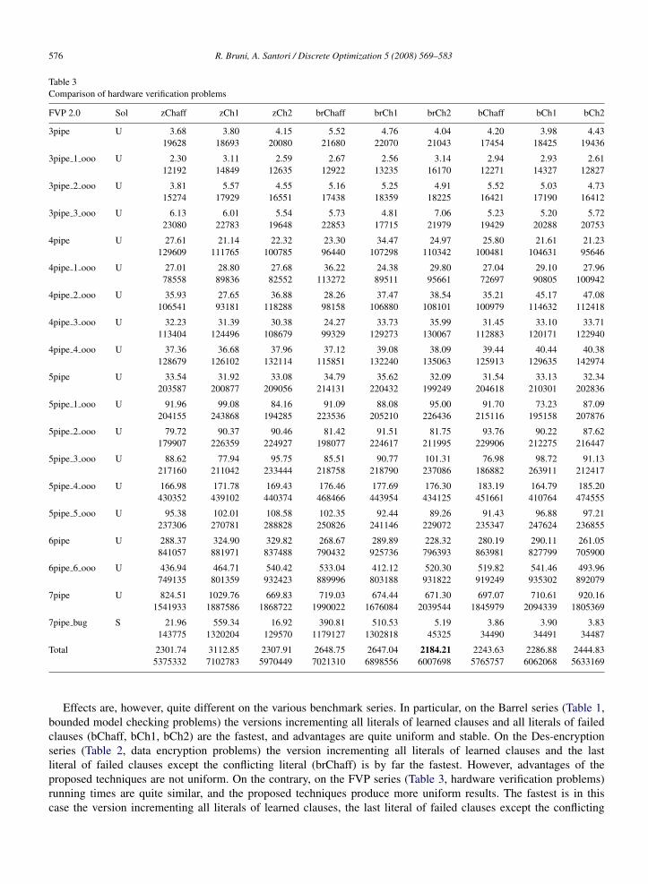
Table 3Comparison of hardware verification problems

FVP 2.0 Sol zChaff zCh1 zCh2 brChaff brCh1 brCh2 bChaff bCh1 bCh2

3pipe U 3.68 3.80 4.15 5.52 4.76 4.04 4.20 3.98 4.4319628 18693 20080 21680 22070 21043 17454 18425 19436

3pipe 1 ooo U 2.30 3.11 2.59 2.67 2.56 3.14 2.94 2.93 2.6112192 14849 12635 12922 13235 16170 12271 14327 12827

3pipe 2 ooo U 3.81 5.57 4.55 5.16 5.25 4.91 5.52 5.03 4.7315274 17929 16551 17438 18359 18225 16421 17190 16412

3pipe 3 ooo U 6.13 6.01 5.54 5.73 4.81 7.06 5.23 5.20 5.7223080 22783 19648 22853 17715 21979 19429 20288 20753

4pipe U 27.61 21.14 22.32 23.30 34.47 24.97 25.80 21.61 21.23129609 111765 100785 96440 107298 110342 100481 104631 95646

4pipe 1 ooo U 27.01 28.80 27.68 36.22 24.38 29.80 27.04 29.10 27.9678558 89836 82552 113272 89511 95661 72697 90805 100942

4pipe 2 ooo U 35.93 27.65 36.88 28.26 37.47 38.54 35.21 45.17 47.08106541 93181 118288 98158 106880 108101 100979 114632 112418

4pipe 3 ooo U 32.23 31.39 30.38 24.27 33.73 35.99 31.45 33.10 33.71113404 124496 108679 99329 129273 130067 112883 120171 122940

4pipe 4 ooo U 37.36 36.68 37.96 37.12 39.08 38.09 39.44 40.44 40.38128679 126102 132114 115851 132240 135063 125913 129635 142974

5pipe U 33.54 31.92 33.08 34.79 35.62 32.09 31.54 33.13 32.34203587 200877 209056 214131 220432 199249 204618 210301 202836

5pipe 1 ooo U 91.96 99.08 84.16 91.09 88.08 95.00 91.70 73.23 87.09204155 243868 194285 223536 205210 226436 215116 195158 207876

5pipe 2 ooo U 79.72 90.37 90.46 81.42 91.51 81.75 93.76 90.22 87.62179907 226359 224927 198077 224617 211995 229906 212275 216447

5pipe 3 ooo U 88.62 77.94 95.75 85.51 90.77 101.31 76.98 98.72 91.13217160 211042 233444 218758 218790 237086 186882 263911 212417

5pipe 4 ooo U 166.98 171.78 169.43 176.46 177.69 176.30 183.19 164.79 185.20430352 439102 440374 468466 443954 434125 451661 410764 474555

5pipe 5 ooo U 95.38 102.01 108.58 102.35 92.44 89.26 91.43 96.88 97.21237306 270781 288828 250826 241146 229072 235347 247624 236855

6pipe U 288.37 324.90 329.82 268.67 289.89 228.32 280.19 290.11 261.05841057 881971 837488 790432 925736 796393 863981 827799 705900

6pipe 6 ooo U 436.94 464.71 540.42 533.04 412.12 520.30 519.82 541.46 493.96749135 801359 932423 889996 803188 931822 919249 935302 892079

7pipe U 824.51 1029.76 669.83 719.03 674.44 671.30 697.07 710.61 920.161541933 1887586 1868722 1990022 1676084 2039544 1845979 2094339 1805369

7pipe bug S 21.96 559.34 16.92 390.81 510.53 5.19 3.86 3.90 3.83143775 1320204 129570 1179127 1302818 45325 34490 34491 34487

Total 2301.74 3112.85 2307.91 2648.75 2647.04 2184.21 2243.63 2286.88 2444.835375332 7102783 5970449 7021310 6898556 6007698 5765757 6062068 5633169

Effects are, however, quite different on the various benchmark series. In particular, on the Barrel series (Table 1,bounded model checking problems) the versions incrementing all literals of learned clauses and all literals of failedclauses (bChaff, bCh1, bCh2) are the fastest, and advantages are quite uniform and stable. On the Des-encryptionseries (Table 2, data encryption problems) the version incrementing all literals of learned clauses and the lastliteral of failed clauses except the conflicting literal (brChaff) is by far the fastest. However, advantages of theproposed techniques are not uniform. On the contrary, on the FVP series (Table 3, hardware verification problems)running times are quite similar, and the proposed techniques produce more uniform results. The fastest is in thiscase the version incrementing all literals of learned clauses, the last literal of failed clauses except the conflicting


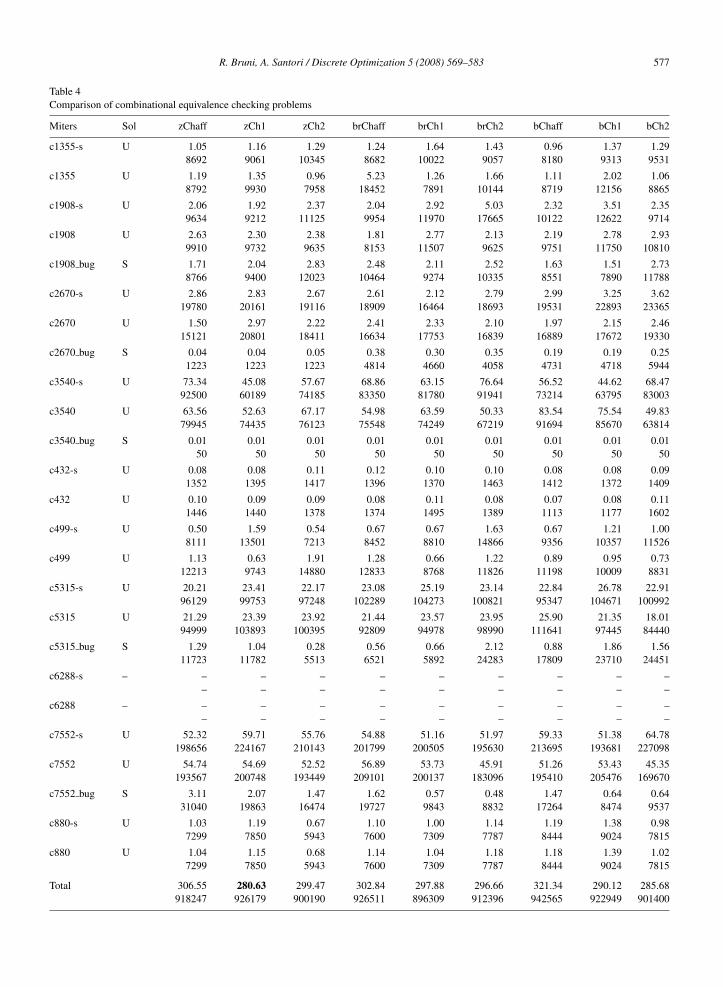
Table 4Comparison of combinational equivalence checking problems

Miters Sol zChaff zCh1 zCh2 brChaff brCh1 brCh2 bChaff bCh1 bCh2

c1355-s U 1.05 1.16 1.29 1.24 1.64 1.43 0.96 1.37 1.298692 9061 10345 8682 10022 9057 8180 9313 9531

c1355 U 1.19 1.35 0.96 5.23 1.26 1.66 1.11 2.02 1.068792 9930 7958 18452 7891 10144 8719 12156 8865

c1908-s U 2.06 1.92 2.37 2.04 2.92 5.03 2.32 3.51 2.359634 9212 11125 9954 11970 17665 10122 12622 9714

c1908 U 2.63 2.30 2.38 1.81 2.77 2.13 2.19 2.78 2.939910 9732 9635 8153 11507 9625 9751 11750 10810

c1908 bug S 1.71 2.04 2.83 2.48 2.11 2.52 1.63 1.51 2.738766 9400 12023 10464 9274 10335 8551 7890 11788

c2670-s U 2.86 2.83 2.67 2.61 2.12 2.79 2.99 3.25 3.6219780 20161 19116 18909 16464 18693 19531 22893 23365

c2670 U 1.50 2.97 2.22 2.41 2.33 2.10 1.97 2.15 2.4615121 20801 18411 16634 17753 16839 16889 17672 19330

c2670 bug S 0.04 0.04 0.05 0.38 0.30 0.35 0.19 0.19 0.251223 1223 1223 4814 4660 4058 4731 4718 5944

c3540-s U 73.34 45.08 57.67 68.86 63.15 76.64 56.52 44.62 68.4792500 60189 74185 83350 81780 91941 73214 63795 83003

c3540 U 63.56 52.63 67.17 54.98 63.59 50.33 83.54 75.54 49.8379945 74435 76123 75548 74249 67219 91694 85670 63814

c3540 bug S 0.01 0.01 0.01 0.01 0.01 0.01 0.01 0.01 0.0150 50 50 50 50 50 50 50 50

c432-s U 0.08 0.08 0.11 0.12 0.10 0.10 0.08 0.08 0.091352 1395 1417 1396 1370 1463 1412 1372 1409

c432 U 0.10 0.09 0.09 0.08 0.11 0.08 0.07 0.08 0.111446 1440 1378 1374 1495 1389 1113 1177 1602

c499-s U 0.50 1.59 0.54 0.67 0.67 1.63 0.67 1.21 1.008111 13501 7213 8452 8810 14866 9356 10357 11526

c499 U 1.13 0.63 1.91 1.28 0.66 1.22 0.89 0.95 0.7312213 9743 14880 12833 8768 11826 11198 10009 8831

c5315-s U 20.21 23.41 22.17 23.08 25.19 23.14 22.84 26.78 22.9196129 99753 97248 102289 104273 100821 95347 104671 100992

c5315 U 21.29 23.39 23.92 21.44 23.57 23.95 25.90 21.35 18.0194999 103893 100395 92809 94978 98990 111641 97445 84440

c5315 bug S 1.29 1.04 0.28 0.56 0.66 2.12 0.88 1.86 1.5611723 11782 5513 6521 5892 24283 17809 23710 24451

c6288-s – – – – – – – – – –– – – – – – – – –

c6288 – – – – – – – – – –– – – – – – – – –

c7552-s U 52.32 59.71 55.76 54.88 51.16 51.97 59.33 51.38 64.78198656 224167 210143 201799 200505 195630 213695 193681 227098

c7552 U 54.74 54.69 52.52 56.89 53.73 45.91 51.26 53.43 45.35193567 200748 193449 209101 200137 183096 195410 205476 169670

c7552 bug S 3.11 2.07 1.47 1.62 0.57 0.48 1.47 0.64 0.6431040 19863 16474 19727 9843 8832 17264 8474 9537

c880-s U 1.03 1.19 0.67 1.10 1.00 1.14 1.19 1.38 0.987299 7850 5943 7600 7309 7787 8444 9024 7815

c880 U 1.04 1.15 0.68 1.14 1.04 1.18 1.18 1.39 1.027299 7850 5943 7600 7309 7787 8444 9024 7815

Total 306.55 280.63 299.47 302.84 297.88 296.66 321.34 290.12 285.68918247 926179 900190 926511 896309 912396 942565 922949 901400


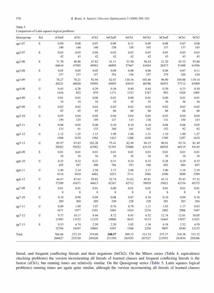
Table 5Comparison of Latin squares logical problems

Quasigroup Sol zChaff zCh1 zCh2 brChaff brCh1 brCh2 bChaff bCh1 bCh2

qg1-07 S 0.09 0.08 0.07 0.09 0.11 0.09 0.08 0.07 0.08140 140 140 158 158 195 137 137 143

qg2-07 S 0.03 0.03 0.04 0.03 0.03 0.03 0.03 0.03 0.0342 43 42 42 42 42 43 43 43

qg2-08 S 71.70 40.86 47.82 41.11 51.50 56.43 21.20 45.32 55.8060619 47505 49563 48895 57467 61654 28473 51409 61956

qg3-08 S 0.05 0.05 0.05 0.09 0.08 0.06 0.06 0.07 0.11157 157 157 354 336 257 279 249 418

qg3-09 U 78.27 70.21 92.94 62.67 110.16 103.46 96.90 104.00 119.1449221 46020 55095 45095 65019 60786 56553 57712 63909

qg4-08 U 0.45 0.26 0.29 0.36 0.40 0.44 0.30 0.33 0.301416 852 879 1171 1333 1347 993 1026 1005

qg4-09 S 0.01 0.01 0.00 0.01 0.00 0.01 0.00 0.01 0.0134 34 34 35 35 35 36 36 36

qg5-09 U 0.02 0.02 0.02 0.02 0.02 0.02 0.02 0.02 0.0265 65 65 66 66 66 66 66 66

qg5-10 U 0.05 0.04 0.04 0.04 0.04 0.04 0.03 0.04 0.04159 125 159 127 133 128 131 150 143

qg5-11 S 0.08 0.05 0.08 0.10 0.10 0.10 0.08 0.06 0.05133 91 133 349 341 342 152 92 92

qg5-12 U 1.12 1.25 1.15 1.09 1.06 1.31 1.10 1.00 1.271508 1670 1584 1423 1288 1638 1389 1297 1610

qg5-13 U 85.97 93.83 102.28 75.41 82.49 94.33 90.91 93.74 81.4958282 59252 63582 51393 55888 63119 60545 60119 54145

qg6-09 S 0.01 0.01 0.01 0.01 0.01 0.01 0.01 0.01 0.0116 16 16 16 16 16 16 16 16

qg6-10 U 0.22 0.22 0.21 0.31 0.24 0.33 0.28 0.29 0.33495 547 490 704 553 548 692 684 697

qg6-11 U 2.40 2.14 2.58 2.73 2.08 2.17 3.00 2.16 2.194116 3419 4462 4251 3711 3584 4396 3690 3399

qg6-12 U 44.47 47.03 59.82 52.74 51.62 45.81 43.31 55.43 57.3237289 41871 44813 42167 42712 39929 35621 42334 45375

qg7-09 S 0.01 0.01 0.01 0.00 0.01 0.01 0.01 0.01 0.018 8 8 8 8 8 8 8 8

qg7-10 U 0.10 0.09 0.09 0.08 0.07 0.10 0.10 0.09 0.10269 269 269 240 226 228 281 263 264

qg7-11 U 0.89 1.09 1.07 0.76 0.79 1.11 1.03 1.17 0.831671 1977 2101 1663 1624 2216 1802 2006 1487

qg7-12 U 9.37 10.17 8.44 8.72 6.93 6.52 12.74 12.01 10.0511993 13152 11235 10806 9433 9133 14443 13957 11421

qg7-13 S 9.53 4.74 2.59 2.20 1.05 1.36 4.18 2.52 4.5932794 18107 10801 4387 1566 2256 9897 6540 12153

Total 304.84 272.19 319.60 248.57 309.33 313.74 275.37 318.38 333.72260427 235320 245628 213350 241955 247527 215953 241834 258386

literal, and frequent conflicting literals and their negations (brCh2). On the Miters series (Table 4, equivalencechecking problems) the version incrementing all literals of learned clauses and frequent conflicting literals is thefastest (zCh1), but running times are relatively similar. On the Quasigroup series (Table 5, Latin squares logicalproblems) running times are again quite similar, although the version incrementing all literals of learned clauses


Table 6Comparison of industrial planning problems

Ferries Sol zChaff zCh1 zCh2 brChaff brCh1 brCh2 bChaff bCh1 bCh2

ferry 5 ks99i S 0.09 0.06 0.06 0.09 0.06 0.09 0.09 0.09 0.091257 1275 1267 1093 1101 1083 1173 1179 1275

ferry 5 v01i S 0.09 0.51 0.06 0.09 0.09 0.09 0.26 0.34 0.20973 4856 913 997 1102 1130 2520 3288 2274

ferry 6 ks99a S 0.09 0.20 0.09 0.14 0.23 0.23 0.20 0.12 0.18704 1181 667 938 1208 1196 1129 686 1129

ferry 6 ks99i S 0.74 0.66 1.21 0.65 0.17 3.49 1.65 0.91 0.127148 6874 10215 6762 3230 16572 11948 9262 2999

ferry 6 v01a S 0.09 0.20 0.20 0.20 0.20 0.20 0.23 0.20 0.17705 1168 1066 1132 1097 1119 1155 1155 1011

ferry 6 v01i S 0.17 0.14 1.60 0.86 1.77 1.54 1.49 0.20 1.001788 1830 10406 7077 12557 10002 9813 2212 6904

ferry 7 ks99a S 0.09 0.06 0.09 0.06 0.09 0.03 0.06 0.06 0.06859 840 838 849 850 872 946 947 939

ferry 7 ks99i S 7.15 5.95 3.43 5.63 4.74 0.17 0.03 0.06 0.0630372 27619 18846 25760 24800 4282 3560 3560 3560

ferry 7 v01a S 0.03 0.01 0.03 0.03 0.03 0.03 0.03 0.01 0.03427 427 427 425 424 424 442 442 445

ferry 7 v01i S 0.51 25.31 4.06 11.32 5.57 9.43 0.86 1.54 1.238610 56654 26116 38862 29490 34315 11073 13382 13164

ferry 8 ks99a S 0.03 0.06 0.03 0.06 0.06 0.06 0.06 0.06 0.121091 1091 1091 1031 992 1084 958 958 1219

ferry 8 ks99i S 8.78 6.46 7.06 8.75 8.43 13.27 32.88 12.72 11.9242296 40972 39414 45256 41061 51134 74253 51431 54193

ferry 8 v01a S 0.06 0.06 0.09 0.09 0.06 0.09 0.09 0.17 0.201181 1188 1429 1014 969 999 1248 2262 2582

ferry 8 v01i S 24.36 19.45 157.65 140.34 1.83 56.93 24.65 139.71 1.7768748 61474 245520 164733 23907 102114 72620 145180 21720

ferry 9 ks99a S 0.03 0.06 0.03 0.06 0.06 0.06 0.06 0.06 0.062457 3323 2457 3589 3578 3578 2975 2969 2959

ferry 9 v01a S 0.06 0.06 0.03 0.03 0.06 0.03 0.03 0.03 0.031870 1874 1869 1731 1731 1731 1355 1349 1349

ferry 10 ks99a S 0.60 0.79 1.83 1.29 0.74 0.43 5.31 6.63 1.544775 8503 9502 7711 6434 4915 20225 4652 9326

ferry 10 v01a S 3.55 1.66 3.95 0.12 6.23 0.20 0.27 0.31 0.1111452 8044 11896 2366 11726 2920 3065 3623 2215

Total 46.52 61.70 181.50 169.81 30.42 86.37 68.25 163.22 18.89186713 229193 383939 311326 166257 239470 220458 248537 129263

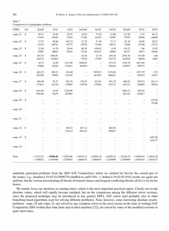
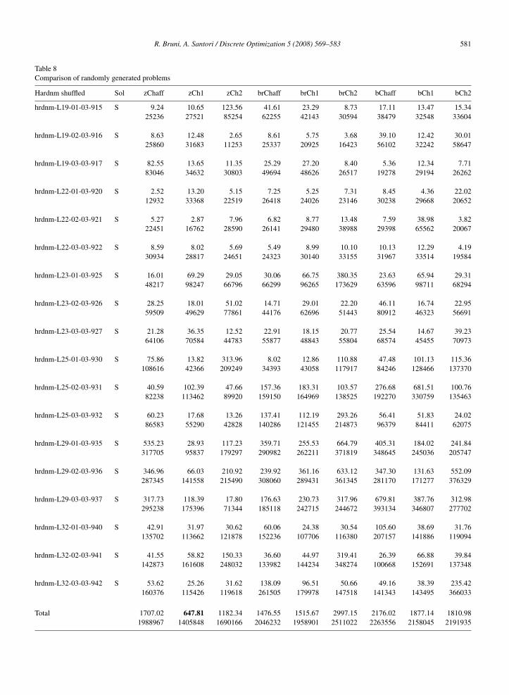
and the last literal of failed clauses except the conflicting literal (brChaff) is again the fastest. On the Ferries series(Table 6, industrial planning problems from the 2005 SAT Competition) the version incrementing all literals oflearned clauses, all literals of failed clauses and both frequent conflicting literals and their negations (bCh2) isby far the fastest, even if results of the various versions are here quite different. On the VMPC inversion series(Table 7, open cryptographic problems from the 2005 SAT Competition) the version incrementing all literals oflearned clauses and frequent conflicting literals (zCh1) is the fastest, even if results of the various versions arehere considerably heterogeneous. Note, in particular, that the version incrementing all literals of learned clauses,all literals of failed clauses and both frequent conflicting literals and their negations (bCh2) is incredibly fast on somedifficult problems of the series, although it has a poor behavior on others. Finally, on the Hardnm series (Table 8,


Table 7Comparison of cryptographic problems

VMPC Sol zChaff zCh1 zCh2 brChaff brCh1 brCh2 bChaff bCh1 bCh2

vmpc 21 S 40.17 35.69 87.07 10.92 73.54 16.98 113.26 4.32 84.1251447 49383 71934 37382 64253 32587 76797 26858 64690

vmpc 22 S 17.27 58.96 167.33 13.75 51.30 71.17 81.26 26.05 20.2741243 66741 97775 29278 51426 68315 71840 47160 31513

vmpc 23 S 23.50 14.70 20.84 80.38 459.02 8.38 139.37 7.46 12.8732087 40043 30101 77444 165147 36982 82271 19977 38440

vmpc 24 S 487.83 1466.91 – 62.56 15.78 295.43 2781.95 191.09 1.00164331 344462 – 72555 27549 124715 453645 98820 6663

vmpc 25 S 45.75 12.04 1212.98 1898.02 – 471.25 1703.79 2677.69 –52606 26166 274411 363854 – 164424 342933 429575 –

vmpc 26 S 683.22 109.23 245.40 – 3078.87 3178.86 – 1037.55 2.53203309 78038 114239 – 491855 486241 – 243033 16153

vmpc 27 S 456.90 55.27 391.76 176.97 415.67 591.35 480.43 859.53 162.13172813 62336 178963 116529 175928 191731 163112 238902 99316

vmpc 28 S 1167.88 34.05 2729.96 – – – 2404.73 892.95 –285294 52479 457885 – – – 387145 242817 –

vmpc 29 S – – – – – – – – 239.96– – – – – – – – 93700

vmpc 30 – – – – – – – – – –– – – – – – – – –

vmpc 31 – – – – – – – – – –– – – – – – – – –

vmpc 32 S – – 198.72 837.14 – 865.82 – – –– – 110112 281415 – 249933 – – –

vmpc 33 S – – – – – – – – 1493.40– – – – – – – – 322177

vmpc 34 – – – – – – – – – –– – – – – – – – –

Total >13722.52 >12586.85 >15854.06 >19454.74 >22094.18 >16299.24 >22104.79 >16496.64 >12816.28>1700422 >1416940 >2204942 >2666253 >2560910 >2230690 >2766890 >2044434 >1841527

randomly generated problems from the 2003 SAT Competition, where we omitted for brevity the central part ofthe names, e.g., hardnm-L19-02-S125896754.shuffled-as.sat03-916→ hrdnm-L19-02-03-916) results are again notuniform, but the version incrementing all literals of learned clauses and frequent conflicting literals (zCh1) is by far thefastest.

We mainly focus our attention on running times, which is the most important practical aspect. Clearly not on theabsolute values, which will rapidly become outdated, but on the comparison among the different solver versions,since the proposed technique may be introduced in any generic DPLL SAT solver (and probably also in otherbranching-based algorithms used for solving different problems). Note, however, some interesting absolute results:problems vmpc 29 and vmpc 32, not solved by any complete solver in the most recent (at the time of writing) SATCompetition 2005 (within their time limit and on their machine) [22], are solved by some of the modified versions inquite short times.


Table 8Comparison of randomly generated problems

Hardnm shuffled Sol zChaff zCh1 zCh2 brChaff brCh1 brCh2 bChaff bCh1 bCh2

hrdnm-L19-01-03-915 S 9.24 10.65 123.56 41.61 23.29 8.73 17.11 13.47 15.3425236 27521 85254 62255 42143 30594 38479 32548 33604

hrdnm-L19-02-03-916 S 8.63 12.48 2.65 8.61 5.75 3.68 39.10 12.42 30.0125860 31683 11253 25337 20925 16423 56102 32242 58647

hrdnm-L19-03-03-917 S 82.55 13.65 11.35 25.29 27.20 8.40 5.36 12.34 7.7183046 34632 30803 49694 48626 26517 19278 29194 26262

hrdnm-L22-01-03-920 S 2.52 13.20 5.15 7.25 5.25 7.31 8.45 4.36 22.0212932 33368 22519 26418 24026 23146 30238 29668 20652

hrdnm-L22-02-03-921 S 5.27 2.87 7.96 6.82 8.77 13.48 7.59 38.98 3.8222451 16762 28590 26141 29480 38988 29398 65562 20067

hrdnm-L22-03-03-922 S 8.59 8.02 5.69 5.49 8.99 10.10 10.13 12.29 4.1930934 28817 24651 24323 30140 33155 31967 33514 19584

hrdnm-L23-01-03-925 S 16.01 69.29 29.05 30.06 66.75 380.35 23.63 65.94 29.3148217 98247 66796 66299 96265 173629 63596 98711 68294

hrdnm-L23-02-03-926 S 28.25 18.01 51.02 14.71 29.01 22.20 46.11 16.74 22.9559509 49629 77861 44176 62696 51443 80912 46323 56691

hrdnm-L23-03-03-927 S 21.28 36.35 12.52 22.91 18.15 20.77 25.54 14.67 39.2364106 70584 44783 55877 48843 55804 68574 45455 70973

hrdnm-L25-01-03-930 S 75.86 13.82 313.96 8.02 12.86 110.88 47.48 101.13 115.36108616 42366 209249 34393 43058 117917 84246 128466 137370

hrdnm-L25-02-03-931 S 40.59 102.39 47.66 157.36 183.31 103.57 276.68 681.51 100.7682238 113462 89920 159150 164969 138525 192270 330759 135463

hrdnm-L25-03-03-932 S 60.23 17.68 13.26 137.41 112.19 293.26 56.41 51.83 24.0286583 55290 42828 140286 121455 214873 96379 84411 62075

hrdnm-L29-01-03-935 S 535.23 28.93 117.23 359.71 255.53 664.79 405.31 184.02 241.84317705 95837 179297 290982 262211 371819 348645 245036 205747

hrdnm-L29-02-03-936 S 346.96 66.03 210.92 239.92 361.16 633.12 347.30 131.63 552.09287345 141558 215490 308060 289431 361345 281170 171277 376329

hrdnm-L29-03-03-937 S 317.73 118.39 17.80 176.63 230.73 317.96 679.81 387.76 312.98295238 175396 71344 185118 242715 244672 393134 346807 277702

hrdnm-L32-01-03-940 S 42.91 31.97 30.62 60.06 24.38 30.54 105.60 38.69 31.76135702 113662 121878 152236 107706 116380 207157 141886 119094

hrdnm-L32-02-03-941 S 41.55 58.82 150.33 36.60 44.97 319.41 26.39 66.88 39.84142873 161608 248032 133982 144234 348274 100668 152691 137348

hrdnm-L32-03-03-942 S 53.62 25.26 31.62 138.09 96.51 50.66 49.16 38.39 235.42160376 115426 119618 261505 179978 147518 141343 143495 366033

Total 1707.02 647.81 1182.34 1476.55 1515.67 2997.15 2176.02 1877.14 1810.981988967 1405848 1690166 2046232 1958901 2511022 2263556 2158045 2191935


We furthermore observe that the number of decisions, for a given problem, is only roughly proportional, and notexactly, to running times. This is because the propagation performed after variable assignments may require differenttimes for different variables, depending on their situation within the formula.

On the contrary, when considering different problems, the ratios between the number of decisions and runningtimes are almost completely unrelated, since, for each decision, time spent in the propagation phase depends heavilyon the size of the problem, and can therefore vary greatly.

5. Conclusions

The branching heuristic has a relevant influence on the computational behavior of DPLL SAT solvers. Conflict-based branching heuristics have the advantages of requiring low computational overhead and of being often able todetect the hidden structure of a problem. We report here a computational study of new scores updating criteria forconflict-based branching heuristics. Such criteria have been developed in order to overcome some of the typical time-wasting behaviors of DPLL search techniques. In particular, the proposed family of conflict-based heuristics has threemain aims: (i) to assign at first the more constrained variables; (ii) to reverse every sequence of assignments whichhave led to a conflict, by satisfying at first clauses which have become empty; and (iii) to assign at first variablesthat, due to their relations with the others, cause frequent backtracks at the same decision level of the search tree.For the above reasons, this family of branching heuristics has been called reverse assignment sequence (RAS). Suchheuristics have been implemented into the state-of-the-art DPLL SAT solver zChaff 2004, obtaining several solverversions having quite different behaviors. Experiments on many benchmark series, both satisfiable and unsatisfiable,show that the proposed branching heuristics are often able to improve solution times. Moreover, notwithstanding thefact that the introduced counter updating requires some computational overhead for its operation, total solution timeson each series are always in favor of one of the new versions of the solver.

As a final remark, the authors suppose that similar score based branching heuristics for guiding the searchperformed by a generic complete branching algorithm can also be adapted to the case of problems different fromthe propositional Satisfiability one.

References

[1] R. Bayardo, R. Schrag, Using CSP look-back techniques to solve real-world SAT instances, in: Proceedings of 14th National Conference onArtificial Intelligence, AAAI, 1997.

[2] R. Bruni, A. Sassano, Restoring satisfiability or maintaining unsatisfiability by finding small unsatisfiable subformulae, in: Proceedings ofTheory and Applications of Satisfiability Testing, SAT2001, 2001.

[3] R. Bruni, A. Santori, Adding a new conflict-based branching heuristic in two evolved DPLL SAT solvers, in: Proceedings of the SeventhInternational Conference on Theory and Applications of Satisfiability Testing, SAT2004, 2004.

[4] M. Buro, H. Kleine Buning, Report on a SAT competition, Bulletin of the European Association for Theoretical Computer Science 49 (1993)143–151.

[5] E. Cervalho, J.P. Marques-Silva, Using rewarding mechanisms for improving branching heuristics, in: Proceedings of the Seventh InternationalConference on Theory and Applications of Satisfiability Testing, SAT2004, 2004.

[6] V. Chandru, J.N. Hooker, Optimization Methods for Logical Inference, Wiley, New York, 1999.[7] S.A. Cook, The complexity of theorem-proving procedures, in: Proceedings of Third Annual ACM Symposium on Theory of Computing,

1971.[8] M. Davis, G. Logemann, D. Loveland, A machine program for theorem proving, Communications of the ACM 5 (1962) 394–397.[9] M. Davis, H. Putnam, A computing procedure for quantification theory, Journal of the ACM 7 (1960) 201–215.

[10] Z. Fu, Y. Mahajan, S. Malik, New features of the SAT’04 version of zChaff, in: SAT 2004 Competition: Solver Descriptions, 2004.[11] M.R. Garey, D.S. Johnson, Computers and Intractability: A Guide to the Theory of NP-Completeness, W.H. Freeman and co., San Francisco,

1979.[12] I.P. Gent, H. van Maaren, T. Walsh (Eds.), SAT 2000, IOS Press, Amsterdam, 2000.[13] E. Goldberg, Y. Novikov, BerkMin: A fast and robust SAT-solver, in: Proceedings of Design Automation & Test in Europe, DATE 2002, 2002.[14] J. Gu, P.W. Purdom, J. Franco, B.W. Wah, Algorithms for the Satisfiability (SAT) Problem: A Survey, in: DIMACS Series in Discrete

Mathematics, American Mathematical Society, 1999.[15] M. Herbstritt, B. Becker, Conflict-based selection of branching rules in SAT-algorithms, in: E. Giunchiglia, A. Tacchella (Eds.), Sixth

International Conference on Theory and Applications of Satisfiability Testing — Selected Papers, in: LNAI, vol. 2919, Springer, 2003.[16] R.E. Jeroslow, J. Wang, Solving propositional satisfiability problems, Annals of Mathematics and AI 1 (1990) 167–187.[17] D. Le Berre, L. Simon, The essentials of the SAT 2003 competition, in: E. Giunchiglia, A. Tacchella (Eds.), Sixth International Conference

on Theory and Applications of Satisfiability Testing — Selected Papers, in: LNAI, vol. 2919, Springer, 2003.[18] P. Liberatore, On the complexity of choosing the branching literal in DPLL, Artificial Intelligence 116 (1–2) (2000) 315–326.


[19] J.P. Marques-Silva, K.A. Sakallah, Conflict analysis in search algorithms for propositional satisfiability, in: Proceedings of IEEE InternationalConference on Tools with Artificial Intelligence, 1996.

[20] J.P. Marques-Silva, The impact of branching heuristics in propositional satisfiability algorithms, in: Proceedings of the 9th PortugueseConference on Artificial Intelligence, EPIA, 1999.

[21] M. Moskewicz, C. Madigan, Y. Zhao, L. Zhang, S. Malik, Chaff: Engineering an efficient SAT solver, in: Proceedings of the 39th DesignAutomation Conference, 2001.

[22] SAT competitions web site, organizers D. Le Berre and L. Simon. http://www.satcompetition.org/; http://www.satlive.org/.[23] K. Truemper, Effective Logic Computation, Wiley, New York, 1998.[24] L. Zhang, S. Malik, The quest for efficient boolean satisfiability solvers, in: Proceedings of CADE 2002 and CAV 2002, 2002.[25] H. Zhang, M.E. Stickel, Implementing the Davis–Putnam method, in: I.P. Gent, H. van Maaren, T. Walsh (Eds.), SAT 2000, IOS Press,

Amsterdam, 2000.

http://www.satcompetition.org/

http://www.satlive.org/

new updating criteria for conflict-based branching heuristics in dpll algorithms for satisfiability

Documents