new strategies of diode laser absorption sensors

NEW STRATEGIES OF DIODE LASER ABSORPTION SENSORS

By

Jian Wang

Report No. TSD-141

August 2001

NEW STRATEGIES OF DIODE LASER ABSORPTION SENSORS

By

Jian Wang

Report No. TSD 141

Work Sponsored By

AFOSR & EPA

High Temperature Gasdynamics Laboratory

Thermoscience Division

Department of Mechanical Engineering

Stanford University

Stanford, California 94305-3032

iii

© Copyright by Jian Wang 2001 All rights reserved

v

Abstract

Diode-laser absorption sensors are advantageous because of their non-invasive nature, fast time

response, and in situ measurement capability. New diode lasers, e.g., GaSb-based longer-

wavelength (> 2 µm) lasers and vertical-cavity surface-emitting lasers (VCSELs) have recently

emerged. The objective of this thesis is to take advantage of these new diode lasers and develop

new gas-sensing strategies.

CO is an important species both as an air pollutant and a key indicator of combustion efficiency.

Using (Al)InGaAsSb/GaSb diode lasers operating near 2.3 µm, in situ measurements of CO

concentration were recorded in both the exhaust (~470 K) and the immediate post-flame zone

(18201975 K) of an atmospheric -pressure flat-flame burner. Using wavelength-modulation

spectroscopy (WMS) techniques, a ~0.1 ppm-m detectivity of CO in the exhaust duct was

achieved with a 0.4-s measurement time. For measurements in the immediate post-flame zone,

quantitative measurements were obtained at fuel/air equivalence ratios down to 0.83 (366-ppm

minimum CO concentration) with only an 11-cm beam path. These results enable many important

applications, e.g., ambient air quality monitoring, in situ combustion emission monitoring, and

engine diagnostics.

As much as 95% of urban CO emission may emanate from vehicle exhaust. The potential of the

2.3-µm CO sensors for on-road remote sensing of vehicle exhaust is examined. A 20-ppm

detectivity for typical 5-cm vehicle tailpipes with a ~1.5-kHz detection bandwidth was

demonstrated in laboratory experiments, implying the potential to monitor CO emissions from

even the cleanest combustion-powered vehicles. Since the temperature profiles of vehicle exhaust

are unknown, non-uniform and quickly varying, a new strategy is proposed to eliminate or

mitigate the constraint of a known or uniform temperature profile along the light beampath. This

new wavelength-multiplexing strategy can be applied to a wide variety of other traditional

absorption spectroscopy-based sensors.

vi

Diode laser absorption is for the first time extended to wavelength-scanning high-pressure gas

detection by exploiting the fast and broad wavelength tunability of some VCSELs. Demonstration

measurements of oxygen in a cell at pressures up to 10 bars are presented. The fast and broad

tunability of laser frequency (>30 cm-1 at 100 kHz) results from the small thermal time constant

associated with small VCSEL cavity volume and the strong resistive heating of distributed Bragg

reflector mirrors. This new strategy is potentially more robust in hostile environments than the

traditional wavelength-multiplexed strategies, and can be easily extended to other species in high-

pressure environments.

vii

Contents Abstract………………………………………………………………………….………… v

Contents……………………………………………………………….…………………… vii

List of Tables……………………………………………………………………………… ix

List of Figures……………………………………………………………………………... x

Chapter 1. Introduction……………………………………………………………… 1

1.1 Motivation and objectives………………………………………………… 1

1.2 Organization of the thesis………………………………………………… 7

Chapter 2. Diode -Laser Absorption Spectroscopy………………………………… 9

2.1 Fundamentals of quantitative absorption spectroscopy… 9

2.2 Direct-absorption spectroscopy…………………………………………… 13

2.3 Modulation spectroscopy………………………………………….……… 16

2.4 Modulation spectroscopy for broadband absorption……………………… 21

Chapter 3. Semiconductor Laser Fundamentals…………………………………… 27

3.1 Achieving gain in semiconductor diode lasers…………………………… 27

3.2 Double heterostructure and quantum wells……………………………….. 34

3.3 Laser structures…………………………………………………………… 36

3.3.1 Edge-emitting lasers……………………………………….……… 36

3.3.2 Surface-emitting lasers…………………………………….……… 40

3.4 Laser dynamics…………………………………………………………… 44

3.5 (Al)InGaAsSb/GaSb diode lasers 51

Chapter 4. In situ CO Detection with 2.3-µµm Lasers……………………………… 55

4.1 Motivation………………………………………………………………... 55

4.2 Candidate transition selections…………………………………………… 57

4.3 Experimental details……………………………………………………… 60

4.4 Linestrength verification…………………………………………………. 62

4.5 Measurements in the exhaust duct…..…………………………………… 64

4.5.1 Direct absorption………………………………………………… 64

4.5.2 Wavelength-modulation spectroscopy…………………………… 66

4.6 Measurements in the immediate post-flame zone………………….…….. 70

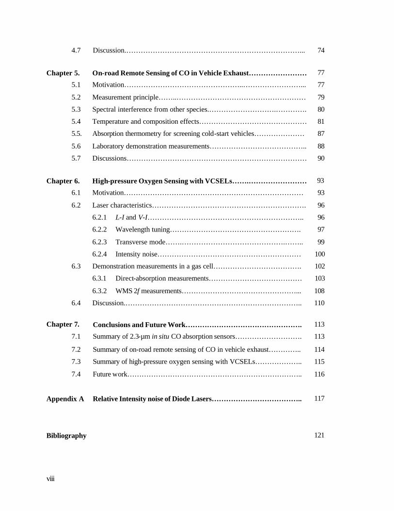
viii

4.7 Discussion.………………………………………………………………... 74

Chapter 5. On-road Remote Sensing of CO in Vehicle Exhaust…………………… 77

5.1 Motivation…………………………………………..……………………... 77

5.2 Measurement principle……..……………………………………………… 79

5.3 Spectral interference from other species.……………………….…………. 80

5.4 Temperature and composition effects……………………………………… 81

5.5. Absorption thermometry for screening cold-start vehicles………………… 87

5.6 Laboratory demonstration measurements………………………………….. 88

5.7 Discussions………………………………………………………………… 90

Chapter 6. High-pressure Oxygen Sensing with VCSELs…….…………………… 93

6.1 Motivation………………………………………………………………… 93

6.2 Laser characteristics………………………………………………………. 96

6.2.1 L-I and V-I……………………………………………………….. 96

6.2.2 Wavelength tuning………………………………………………. 97

6.2.3 Transverse mode…….…………………………………….…….. 99

6.2.4 Intensity noise…………………………………………………… 100

6.3 Demonstration measurements in a gas cell………………………………. 102

6.3.1 Direct-absorption measurements………………………………… 103

6.3.2 WMS 2f measurements…………………………………………... 108

6.4 Discussion.……………………………………………………………….. 110

Chapter 7. Conclusions and Future Work…………………………………………. 113

7.1 Summary of 2.3-µm in situ CO absorption sensors………………………. 113

7.2 Summary of on-road remote sensing of CO in vehicle exhaust………….. 114

7.3 Summary of high-pressure oxygen sensing with VCSELs……………….. 115

7.4 Future work……………………………………………………………….. 116

Appendix A Relative Intensity noise of Diode Lasers……………………………….. 117

Bibliography 121

ix

List of Tables Chapter 4

Table 4.1

Fundamental spectroscopic data of the CO R(15) and R(30) transitions

( 0''v2'v =←= )…………………………………………………………….

59

Table 4.2 HITRAN96 coefficients of the polynomial ( TdTcbTaTQ 32)( +++= )

for the partition function of CO……………………………………………….

60

Chapter 5

Table 5.1

California CO emission standards (g/mile) for 2001 and subsequent model

passenger cars (California Environmental Protection Agency Air Resources

Board 1999)…………………………………………………………………..

90

Table 5.2 Summary of the differences between the new and the traditional sensing

strategies………………………………………………………………………

91

Chapter 6

Table 6.1

Linestrengths and broadening coefficients of the R5Q6, R7R7 and R7Q8

transitions in the oxygen A band at 293 K……………………………………

107

x

List of Figures Chapter 1

Figure 1.1

Bandgap energy and wavelength vs. lattice constant of some III-V

semiconductor compounds and alloys……...………………………………...

2

Figure 1.2 Worldwide sales of diode lasers by application……………………………... 4

Chapter 2

Figure 2.1 Schematic of typical direct-absorption measurements………………………. 14

Figure 2.2 Sample signal obtained by passing through a gas media ……………………. 15

Figure 2.3 Sample etalon signal trace. The peak-peak frequency spacing is the free

spectral range (FSR) of the etalon……………………………………………

15

Figure 2.4 Obtained absorbance trace in the frequency domain is fitted to a theoretical

lineshape to yield the gas concentration……………………………………...

16

Figure 2.5 Shape of WMS 2f trace with different modulation indices………………….. 20

Figure 2.6 Modulation technique for detecting species with broadband absorption……. 22

Figure 2.7 Spectral view of the standard frequency modulation spectroscopy…………. 25

Chapter 3

Figure 3.1 A generic edge-emitting laser cavity cross section showing active and

passive sections and the guided mode profile ..………………………….….

27

Figure 3.2 Illustration of the band edges of a homojunction diode (a) at equilibrium

and (b) under forward bias. (b) shows that the electron and hole quasi-

Fermi levels FhE and FeE approximately continues into the depletion

region and decrease into the N and P regions……………………………….

29

Figure 3.3 Band-to-band stimulated absorption and emission…………………………. 30

Figure 3.4 State pairs which interact with photons with energy E21 (E2-E1) for

stimulated transitions………………………………………………………..

31

Figure 3.5 Conduction-band structure of one period of a quantum-cascade laser……... 33

Figure 3.6 Aspects of the double -heterostructure diode laser: (A) a schematic of the

material structure; (B) an energy diagram of the conduction and valence

bands vs. transverse distance; (C) the refractive index profile; (D) the

electric filed amplitude profile for a laser mode…………………………….

35

xi

Figure 3.7 Transverse band structure for a standard separate-confinement

heterostructure (SCH) quantum-well laser……………………………….…

36

Figure 3.8 Illustration of the divergence of a laser beam in the vertical and horizontal

directions from an edge-emitting laser……………………………………...

37

Figure 3.9 A distributed Bragg reflector laser structure……………………………….. 38

Figure 3.10 (a) Standard distributed feedback (DFB) laser structure (b) quarter-wave

shifted DFB structure………………………………………………………..

39

Figure 3.11 Schematic illustration of how a single axial mode is selected in an edge-

emitting or a VCSEL laser…………………………………………………..

40

Figure 3.12 Schematic of a VCSEL structure. ………………………….………………. 41

Figure 3.13 Double intracavity contacted 1.5 µm single mode VCSEL………………… 42

Figure 3.14 1.3-µm InGaAsN VCSEL with AlGaAs DBRs…………………………….. 43

Figure 3.15 Conservation of carriers and photons used in the rate-equation analysis of

semiconductor lasers………………………………………………………..

45

Figure 3.16 Illustration of the modulation transfer function ( )H ω …………………….. 49

Figure 3.17 Wavelength vs. temperature characteristics for an InGaAsSb/AlGaAsSb

laser (0.25-mm cavity length) at a fixed current (90 mA). The inset shows

the lasing spectra acquired at 18.5oC..………………………………………

52

Figure 3.18 Temperature and current dependences of a single-mode operation

region…………………………………………………………………

54

Chapter 4

Figure 4.1 Survey spectra of CO and major combustion products H2O and CO2 at 500

K based on HITRAN96 database…

56

Figure 4.2 Calculated spectra of H2O (10%) and CO (10 ppm) at 500 K, 1 atm based

on HITRAN96 parameters ………………………….………………………

58

Figure 4.3 Calculated spectra of H2O (10%), CO2 (10%), and CO (500 ppm) at 1500

K, 1 atm based on HITEMP96 parameters…..……………………………...

59

Figure 4.4 Calculated linestrength and corresponding relative temperature sensitivities

of the CO R(15) and R(30) transitions as a function of temperature………..

60

Figure 4.5 Schematic diagram of the experimental setup for in situ CO measurements

in the exhaust and immediate post-flame regions of a flat-flame burner…...

61

xii

Figure 4.6 Measured integrated areas (per centimeter beam path) at various pressures

for the CO R(15) and R(30) transitions……………………………………..

63

Figure 4.7 Measured CO lineshape (R(15) transition, 50-sweep average) recorded in

the exhaust duct (XCO = 22 ppm, φ�= 0.97, T ~ 470 K, L = 120 cm)………...

64

Figure 4.8 Measured CO concentrations recorded using direct-absorption

spectroscopy in the exhaust duct (T~470 K, P=1atm) as a function of

equivalence ratio…………………………………………………………….

65

Figure 4.9 Schematic diagram for CO measurements in the exhaust duct using WMS

techniques…………………………………………………………………...

66

Figure 4.10 Representative 2f lineshapes (~1.46 modulation index, 20-sweep average)

for CO measurements in the exhaust duct…………………………………..

67

Figure 4.11 Measured CO concentrations in the exhaust duct using wavelength-

modulation spectroscopy (2f) techniques (2.5-Hz measurement repetition

rate). The inset shows the time variation of CO concentration (φ=0.53)

recorded with 100-Hz measurement repetition rate……………

69

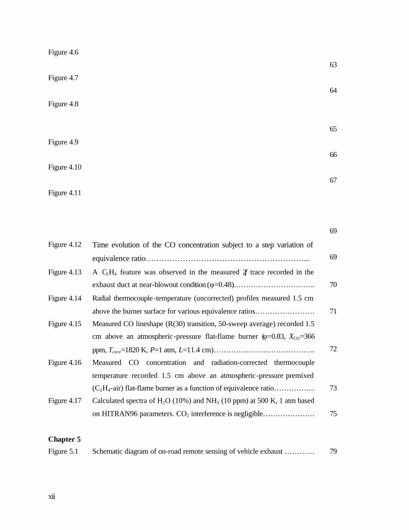
Figure 4.12 Time evolution of the CO concentration subject to a step variation of

equivalence ratio……………………………………………………...

69

Figure 4.13 A C2H4 feature was observed in the measured 2f trace recorded in the

exhaust duct at near-blowout condition (φ=0.48).…………………………..

70

Figure 4.14 Radial thermocouple-temperature (uncorrected) profiles measured 1.5 cm

above the burner surface for various equivalence ratios……………………

71

Figure 4.15 Measured CO lineshape (R(30) transition, 50-sweep average) recorded 1.5

cm above an atmospheric -pressure flat-flame burner (φ=0.83, XCO=366

ppm, Tcore=1820 K, P=1 atm, L=11.4 cm)…………………………………..

72

Figure 4.16 Measured CO concentration and radiation-corrected thermocouple

temperature recorded 1.5 cm above an atmospheric-pressure premixed

(C2H4-air) flat-flame burner as a function of equivalence ratio……………..

73

Figure 4.17 Calculated spectra of H2O (10%) and NH3 (10 ppm) at 500 K, 1 atm based

on HITRAN96 parameters. CO2 interference is negligible…………………

75

Chapter 5

Figure 5.1 Schematic diagram of on-road remote sensing of vehicle exhaust ………… 79

xiii

Figure 5.2 Temperature dependence of the normalized linestrengths of several CO

transitions (2v band) free from H2O interference …………………………..

83

Figure 5.3 Temperature dependence of the normalized linestrengths of the CO R(15)

transition and some CO2 transitions.…………….………………………….

84

Figure 5.4 Calculated temperature factors for the best single -transition (J”=38 or 40)

and some two-transition CO2-measurement combinations………………….

85

Figure 5.5 Calculated normalized collisional linewidths of the CO R(15) transition

and CO2 transitions (J”=22,48) with different initial exhaust-gas

temperatures (Tini)………………………………………………………..….

86

Figure 5.6 Ratio of measured CO2 column densities with different transition pairs as a

function of temperature, Tref=300 K ………………………………………..

88

Figure 5.7 Measured CO effluent (1.5-kHz detection bandwidth, 100-Hz

measurement repetition rate) in the exhaust duct (470 K) at an equivalence

ratio of 0.53. The inset shows one representative measured lineshape……..

89

Figure 5.8 Schematic of the traditional and the proposed new sensing strategies …….. 91

Chapter 6

Figure 6.1 Tunable VCSEL developed by Bandwidth9………………………………... 95

Figure 6.2 Light output versus current (L-I) characteristics at different heat-sink

temperatures and operation voltage versus current (V-I) characteristics at a

heat-sink temperature of 25 oC for a 760-nm VCSEL. …………………….

96

Figure 6.3 Quasi-static optical-frequency tuning by varying injection current

and heat-sink temperature………………………...…………………….

98

Figure 6.4 The optical-frequency tuning range as a function of ramp-current

modulation frequency characterized by an etalon. The inset shows one

specific etalon trace obtained at a modulation frequency of 10 kHz………..

99

Figure 6.5 Higher-order transverse mode appears at high pumping levels (>7.5 mA)

and can be suppressed by increasing heat-sink temperature ……………….

100

Figure 6.6 Measured laser rela tive intensity noise (RIN) as a function of output

power. The inset shows RIN versus frequency characteristic recorded at a

bias current of 10 mA and a heat-sink temperature of 40 oC…...…………...

102

xiv

Figure 6.7 The experimental setup for high-pressure oxygen measurements.

The reference beam was only used for direct-absorption

measurements……………………………………………………………...

103

Figure 6.8a 50-sweep-averaged examples (~10-cm-1 frequency tuning) of transmitted

and incident laser intensities recorded at a pressure of 10.9 bar and a

temperature of 293 K………………………………………………………..

106

Figure 6.8b The top panel shows the reduced quasi-absorbance and a least-squares

multi-transition Lorentzian fit. The bottom panel gives the fitting residual...

106

Figure 6.9 Sample single-sweep 2f traces recorded at different pressures with a

constant wavelength modulation (~0.31 cm-1 peak amplitude)……………..

109

1

Chapter 1. Introduction 1.1 Motivation and objectives Compared with some traditional sampling-based gas-sensing instruments, e.g.,

chemiluminescence-based analyzers, gas-sensing systems based on in situ laser absorption

spectroscopy are non-invasive, exhibit fast time response, and can yield absolute measurements.

Furthermore, the line-of-sight measurement principle inherently gives line-averaged

measurements, which can be beneficial in elucidating the overall nature of a gas flow. However,

for these systems to be widely deployed in industrial applications, rather than just delicate and

expensive laboratory equipment, suitable laser sources are needed.

In contrast to other bulk lasers, semiconductor diode lasers are easy to use, free of maintenance,

rugged, and low cost. They also have very low intensity noise, which is essential for achieving

high sensitivity. In addition, their wavelength can be directly tuned by changing injection current

to scan over the entire lineshape of an absorption transition. Therefore, they are attractive sources

for industrial gas-sensing applications. However, not all diode lasers are suitable for high-

resolution absorption spectroscopy.

First of all, diode lasers with the specific wavelength that can access the candidate

spectroscopic transition of the species to be measured are required for absorption-spectroscopy

sensors. To first order, the photon energy emitted by semiconductor diode lasers is equal to the

bandgap energy of the semiconductor material. Therefore, to obtain a specific laser wavelength, a

semiconductor material with the right bandgap energy needs to be selected. In addition, almost all

diode lasers are based on heterostructures, and the lattice constants of semiconductor materials

control the heterostructures that can be made. In most cases, to grow one crystalline material on

another successfully, their lattice constants need to be very close. Otherwise, the grown material

may have a large number of crystalline defects, which will often stop the devices from

functioning as desired. Figure 1.1 illustrates the bandgap energies and lattice constants of some

III-V semiconductor materials, which have made a significant scientific and technological impact

(Woodall 1980; Razeghi 2000). III-V diode lasers can potentially cover a wavelength range from

the deep ultraviolet (~200 nm) to the midinfrared (~5 µm). III-V based quantum-cascade (QC)

semiconductor lasers (they are not diode lasers, see details in chapter 3) can even extend the

wavelength range to longer than 10 µm. III-nitrides (not shown in the figure 1.1) can potentially

Chapter 1

2

allow a wide wavelength range from ~200 nm to ~600 nm, though only a very small range of

390-410 nm is commercially available. The AlGaAs/GaAs system has a very good lattice match,

and is used to make, e.g., 780-nm lasers for compact-disk players and 850-nm lasers for short-

distance data communications. The InGaAs/GaAs system can be used to make strained quantum

well lasers at 980 nm for pumping erbium-doped amplifiers. The InGaAsP/GaAs system can be

used to obtain Al-free laser diodes covering a wide wavelength range of 630-870 nm. One very

important application of this system is to make the 808-nm pump lasers for Nd:YAG lasers.

InGaAsP/InP and InGaAlAs/InP material systems can cover the 1.3-µm and 1.5-µm bands for

fiber optical communications. The above material systems are relatively mature and lasers from

these materials are usually very reliable.

Figure 1.1 Bandgap energy and wavelength vs. lattice constant of some III-V

semiconductor compounds and alloys.

To detect trace gases such as nitric oxide (NO) and carbon monoxide (CO), diode lasers which

can access their absorption transitions of large linestrength are desired. Typically, electronic

transitions and transitions in fundamental or first-overtone vibrational bands have relatively

strong linestrength. However, electronic transitions are typically in the ultraviolet (UV) or deep

UV regions. Though it is potentially possible to reach the UV region with nitride-based diode

lasers, the available wavelength range is currently rather limited (~390-410 nm), and the

Introduction

3

extension of the wavelength range to UV or deep UV is still under research and development. On

the other hand, the fundamental and first-overtone vibrational transitions are typically in the mid-

infrared region. Some of this wavelength region can be reached by the III-V based lasers, e.g., the

(Al)InGaAsSb/GaSb lasers (figure 1.1).

CO is a very important species, both as an air pollutant and a good indicator of combustion

efficiency (Wang et al. 2000a). There is thus a strong need for sensitive in situ CO sensors. The

1.5-µm band “telecom” (telecommunication) lasers can access the CO second-overtone band.

However, since the linestrength is very weak and there is also relatively large spectral

interference from other species, sensitive in situ detection is very difficult. Therefore, longer-

wavelength lasers which can access the stronger transitions in the first-overtone band at 2.3 µm or

the fundamental band at 4.6 µm are desired. Diode lasers based on InGaAsP/InP and

InGaAlAs/InP material systems are very difficult to extend beyond 2 µm. However, 2.3-µm

(Al)InGaAsSb/GaSb diode lasers have been successfully demonstrated to operate in a

continuous-wave mode and around room temperature (Garbuzov et al. 1999). These lasers

provide the opportunity to detect CO with its first-overtone transitions, and very good in situ

sensitivity can potentially be achieved. The first part of this thesis has been devoted to exploring

this new strategy of CO measurement by taking advantage of new lasers developed by Sarnoff

Corporation and Sensors Unlimited Inc.. The lasers obtained were research-grade prototypes and

had poor reliability (lifetime ranged from several minutes to several hundred hours for the over

20 lasers tested). Therefore, significant reliability issues must be addressed before these lasers can

be employed for long-term in-field applications. Although both of these companies recently

decided to focus on the telecom market and quit the smaller gas-sensing business, it is hoped that

the high potential for CO measurements at 2.3 µm demonstrated here will serve to stimulate new

sources for these lasers.

Vehicle exhaust is the biggest CO source in urban areas. Indeed this accounts for more than

ninety percent of total CO emissions in urban areas. Monitoring the emission status of each

individual vehicle is one strategy for controlling this biggest emission source. The generally

adopted monitoring strategy, i.e., infrequent smog checks, has been identified to have some

serious drawbacks. On-road remote sensing is considered to be an important supplemental

strategy. Though there is a need for on-road remote sensing, relatively little attention has been

paid to this important field by the diode-laser gas-sensing community. It is much more difficult to

monitor distributed mobile pollution sources on the road than to monitor stationary sources. The

Chapter 1

4

exhaust from vehicle tailpipes quickly disperses in the air, and thus the gas temperature and

composition quickly evolve. Therefore, fast time response is required to yield accurate

measurements. In addition, exhaust from different vehicles has different, non-uniform, and

unknown concentration and temperature profiles. Absorption spectroscopy is a line-of-sight

technology, and quantitative measurements generally require a uniform concentration profile and

a known or uniform temperature profile along the light beam path. Therefore, traditional

absorption-spectroscopy techniques are not appropriate for this application. Hence, another goal

of this thesis is to develop a new strategy to mitigate or eliminate the abovementioned constraints

and thus significantly extend the application domain of absorption spectroscopy.

The worldwide market for diode lasers reached the stratospheric level of $6.59 billion in 2000

(figure 1.2). This figure represents a growth rate of 108% over the $3.17 billion reported for

1999, which is the largest increase ever recorded for the diode laser market (Steele 2001). Clearly

telecom is by far the largest market, driven by insatiable requirements for bandwidth.

Unfortunately, instrumentation and sensing account for the smallest, almost negligible, diode

laser market.

Figure 1.2 Worldwide sales of diode lasers by application. (Laser Focus World,

February 2001).

The huge market of telecom lasers keeps attracting diode-laser manufacturers to quit the gas-

sensing business and to focus on the telecom market. It is becoming increasingly difficult to find

Introduction

5

lasers of non-telecom wavelength, though some companies in Europe and Japan still manufacture

diode lasers for spectroscopic applications. On the other hand, the stringent requirements and the

strong competition on the telecom lasers continuously drive the advancement of every aspect of

laser technology: laser structure, material growth, and processing. This advancement of the laser

technology and other aspects of lightwave communication technologies such as fiber-optic

technology will eventually benefit the gas-sensing community.

For example, telecom lasers are likely to eventually cover a larger wavelength range to deliver

more bandwidth. Traditionally, telecom diode lasers operate in either the 1.3-µm band or the 1.5-

µm band for transmission because of the low attenuation of silica-based fiber at these

wavelengths. The 1.4-µm band has not been available because of higher attenuation (1dB/km or

higher) of the silica-based fiber. However, technology for fiber manufacturing has been

significantly improved recently. The water concentration in some fiber, e.g., Lucent Technologies

AllWaveTM optical fiber, can be made so low that the entire range of 1285 nm to 1625 nm can

now be used for laser transmission with reasonably low attenuation. Therefore, telecom-grade

lasers will likely be available over this larger wavelength range in the near future to take full

advantage of these new fibers. Many important gas species have transitions in this wavelength

range, and thus this extension of telecom wavelength range can certainly be valuable to the gas-

sensing community.

In addition to the wavelength requirement, diode lasers for gas sensing based on spectroscopic

techniques need to operate in single -axial and single-transverse mode. The side-mode suppression

ratio (SMSR) usually needs to be better than 20 dB. This typically precludes the use of cheap

Fabry-Perot lasers, e.g., those used for data storage or entertainment applications, in long-term in-

field gas-sensing applications, because these lasers typically have low SMSR and exhibit mode-

hop behavior. More expensive distributive feedback (DFB) and distributive Bragg reflector

(DBR) lasers are traditionally used for commercial gas sensors, though FP lasers may be used in

laboratory research environments. In the past decade, significant advancement has been made in

the technology of vertical-cavity surface-emitting lasers (VCSELs), mainly driven by telecom and

interconnection applications. These lasers are inherently low cost due to their good

manufacturability and high yield, on-wafer testing capability, low beam divergence and thus easy

fiber-pigtailed packaging. Single-axial-mode operation is intrinsically obtained due to VCSELs’

extremely short effective cavity length (one to several wavelengths). With careful transverse-

Chapter 1

6

mode control, single-transverse-mode operation can be simultaneously achieved. Therefore,

VCSELs can also satisfy the SMSR requirement for gas-sensing applications.

Currently, VCSELs are only commercially available with a very limited wavelength range

(~0.7-1 µm). However, many research institutes and companies are actively developing VCSELs

in the 1.3-µm and 1.5-µm bands for telecom applications (Coldren et al. 2001; Harris 2000;

Chang-Hasnain 2000). Once they are commercially available, these cheap and single -mode lasers

with low beam divergence will certainly find their applications in and make great impact on the

gas-sensing field. Furthermore, electrically-pumped VCSELs operating near 2.2 µm (Baranov et

al. 1998) and optically-pumped mid-infrared (~2.9 µm) VCSELs (Bewley et al. 1999) have been

successfully demonstrated with Sb-based materials. However, it may take much longer time for

these VCSELs to be of commercial grade due to the significantly less investment compared to

that on telecom VCSELs. Finally, because of the small active volume of VCSELs, their thermal

load and time constant are significantly smaller than those of edge-emitting lasers. These

characteristics enable fast and large wavelength tuning. This special property of VCSELs has

been exploited for the first time in this thesis to develop a new wavelength-scanning scheme

suited for high-pressure gas sensing.

The overall objective of this thesis is to develop new strategies and to extend the application

domains of absorption gas sensing by taking advantage of the new diode lasers which have

emerged in the past few years. Specific objectives of this thesis are the following:

1. Investigate the new 2.3-µm Sb-based diode lasers for combustion diagnostics

applications. The best transitions that are free from interference and have minimum

temperature sensitivity were identified. The linestrength of these transitions were verified

with static gas-cell measurements. Then the experiment was conducted in the low-

temperature (~470 K) exhaust duct and the immediate post-flame zone (1820-1975 K) of

an atmospheric -pressure flat-flame burner.

2. Extend the application of the developed 2.3-µm CO sensor to on-road remote monitoring

of vehicle exhaust. Special complications of this application were identified and a new

gas sensing approach was proposed to overcome these complications.

3. Develop a wavelength-scanning technique for high-pressure oxygen gas sensing by

exploiting the large and fast wavelength tunability of some 760-nm VCSELs. The origin

of this large and fast tunability and other laser characteristics of importance to gas

sensing were studied.

Introduction

7

1.2 Organization of the thesis

The fundamentals of high-resolution absorption spectroscopy are introduced in Chapter 2. Both

direct absorption and modulation spectroscopy are discussed. Chapter 3 presents some

fundamentals of diode lasers. Characteristics of different laser structures are described, and the

basics of laser dynamics relevant to wavelength-modulation spectroscopy are also given. The

application of Sb-based 2.3-µm lasers in detecting carbon monoxide is discussed in Chapter 4.

The main findings of both exhaust and immediate post-flame zone measurements are presented in

detail. Chapter 5 explores the application of diode-laser sensors to on-road vehicle-exhaust

sensing. A new temperature- and composition-insensitive technique is proposed to overcome the

complication of unknown environment parameters encountered in these applications. Chapter 6

presents the application of 760-nm VCSELs to high-pressure oxygen sensing with the oxygen A-

band transitions. Chapter 7 summarizes the thesis and suggests future work. Appendix A

provides the physical background and measurement method of diode-laser relative intensity noise

(RIN).

Chapter 1

8

9

Chapter 2. Semiconductor Laser Absorption Spectroscopy Diode-laser absorption spectroscopy advantageously offers in situ gas-sensing capability in

hostile environments. With its reasonably good sensitivity and relatively simple realization,

diode-laser absorption spectroscopy finds widespread industrial applications (Allen 1998).

Essentials of quantitative absorption spectroscopy for measuring gas concentration are first

introduced. This thesis used two techniques of diode-laser absorption spectroscopy: direct-

absorption spectroscopy and modulation spectroscopy. Their essential characteristics will be

discussed in the following sections.

2.1 Fundamentals of quantitative absorption spectroscopy

The fractional transmission, )í(T , of the effectively monochromatic semiconductor laser

radiation at frequency ν [cm-1] through a gaseous medium of length L [cm] may be described by

the Beer-Lambert relationship:

0

(í ) exp( ( ) )L

o v

IT k x dx

Iν

= = −∫ , (2.1)

where kν [cm-1] is the spectral absorption coefficient; I and Io are the transmitted and incident

laser intensities. The spectral absorption coefficient kν [cm-1] comprising Nj overlapping

transitions in a multi-component environment of K species can be expressed as

,,1 1

( )jNK

j i jv i jj i

P Tk SXÖ= =

= ∑ ∑ , (2.2)

where P [atm] is the total pressure, Xj is the mole fraction of species j, Si,j [cm-2 atm-1] and Φi,j

[cm] are the linestrength and lineshape of a particular transition i of the species j, respectively.

The lineshape function Φi,j is normalized such that

, ( , í) í 1i j x dÖν ≡∫ . (2.3)

Broadening mechanisms can be classified as either homogeneous or inhomogeneous.

Homogeneous broadening mechanisms affect all molecules equally, while inhomogeneous

broadening mechanisms affect some subgroups of molecules differently than others. The

dominant homogeneous broadening mechanism in this thesis is collisional interactions with other

molecules, resulting in a Lorentzian lineshape profile,

Chapter 2

10

( )2

2

0

1(í )

2

2

CC

CS

Öν

π νν ν ν

∆=∆ +− −∆

, (2.4)

where Cν∆ represents the collision width (FWHM, full width at half the maximum), Sν∆ is the

collision shift, and 0ν is the linecenter frequency. In the limit of binary collisions the collision

width and shift are proportional to pressure at constant temperature and, for multi-component

environments, the total collisional linewidth and shift may be obtained by summing the

contribution from all components:

2 )(C j jj

P Xν γ∆ = ∑ , (2.5)

)( jS jj

P Xν δ∆ = ∑ , (2.6)

where Xj is the mole fraction of component j, γj [cm-1 atm-1] and δj [cm-1 atm-1] are the collisional

broadening and shift coefficients due to perturbation by the jth component. Both the collisional

broadening coefficient and shift coefficient are functions of temperature, and simple power laws

may be used to describe these dependences:

0 0j

Tj j

nT T

Tγ γ =

, (2.7)

0 0jm

T Tj j

TT

δ δ =

, (2.8)

where T0 is the reference temperature, nj and mj are corresponding temperature exponents. The

temperature exponents are weak functions of temperature and are generally smaller for higher

temperature ranges.

The collision-caused frequency shift is negligible compared with the typical tuning range of

semiconductor diode lasers even at very high pressures. Therefore, if a wavelength-scanning (the

wavelength is scanned over the entire transition feature) scheme is used, the frequency shift due

to collision has no effect on measuring gas concentrations. However, if there are multiple

transitions in the probed spectral range, then the frequency spacings between neighboring

transitions at high pressures may be different from their values reported in the literature and

databases based on low pressures due to the different shift coefficients of different transitions.

Consequently, the relative frequencies of these transitions are usually set as variables to be

optimized in the data fitting routine for high-pressure gas sensing.

Semiconductor Laser Absorption Spectroscopy

11

Theoretically, to calculate the collision linewidth of a transition in an N-component

environment, we need to know 2N spectroscopic data (N different broadening coefficients γTj

0 , N

different temperature exponents nj) and N+1 environment parameters (N partial pressures of

different components and gas temperature T). Practically, only parameters of those major

components matter, because the contribution of different components is weighted by their mole

fractions (Eq. (2.5)). Even so, this sometimes prevents the successful application of modulation

spectroscopy, which generally requires accurate knowledge of the transition linewidth at the

measurement conditions.

Doppler broadening is the dominant inhomogeneous broadening mechanism and results from

the different Doppler frequency shift of each velocity class of the molecular velocity distribution.

If the velocity distribution is Maxwellian, the resulting lineshape corresponds to a Gaussian

profile,

∆−

−∆

=ΦDD

D ν

νν

πνν 0

2

2ln4exp2ln2

)( , (2.9)

where Dν∆ represents the Doppler width (FWHM), which is calculated using

1 2707.1623 ( / )10D T Mν ν−∆ = × , (2.10)

where 0ν [cm-1] is the linecenter frequency, T [K] is the absolute temperature, and M [a.m.u] is

the molecular weight of the probed species. In contrast to collision linewidth, we only need to

know the gas temperature to calculate Doppler linewidth.

If Doppler and collisional broadening are of similar magnitude, the resulting lineshape can be

modeled as a Voigt profile (Varghese and Hanson 1981a), which is a convolution of Lorentzian

and Gaussian profiles:

duuu CD )()()( −Φ∫ Φ=Φ+∞

∞−νν , (2.11)

assuming two broadening mechanisms are independent. Defining the Voigt a parameter as

D

Caν

ν

∆∆

=2ln

0 . (2.12)

and a non-dimensional line position w as

02 ln2( )S

D

wν ν ν

ν− − ∆

=∆

, (2.13)

The Voigt profile can be calculated as

Chapter 2

12

),()0()( waVDΦ=Φ ν , (2.14)

where (0)DΦ represents the magnitude of the Doppler profile at linecenter, and V(a,w) is the

Voigt function, which can be calculated with many numerical algorithms with different accuracy

and efficiency (e.g., Armstrong 1967; Whiting 1968; Drayson 1976; Humlicek 1982; Ouyang and

Varghese 1989; Schreier 1992).

The transition linestrength, which reflects the net result of both absorption and stimulated

emission, depends on optical transition probability and lower- and upper-state molecular

populations. The optical transition probability is a fundamental parameter, dependent only on the

wavefunctions of the lower and upper states, and thus is not a function of temperature. However,

the lower- and upper-state populations are functions of temperature. Within the work of this

thesis, local thermal equilibrium can be safely assumed, and thus the molecular population

distribution among different energy states is solely determined by the local gas temperature. At

the temperature and pressure ranges encountered in this thesis, population distribution is always

in the non-degenerate limit and can be satisfactorily described by the Boltzmann statistics.

In some spectroscopic databases such as HITRAN96 (Rothman et al. 1998) linestrength is

given in unit of cm/molecule, i.e., on a per molecule basis. Although this is a more fundamental

presentation, it is not very convenient to use in the context of gas concentration measurements

where pressure or mole fraction rather than molecule number is often used. Therefore, in the gas-

sensing community linestrength is typically expressed in a unit of cm-2 atm-1, i.e., on a per

atmosphere pressure basis. The conversion is

2 13

[ ]( )[ ] ( )[ / ]

[ ]

N moleculeS T S T cm moleculecm atm

PV cm atm− − = ⋅

3

7.34 21( )[ / ]

[ ]

e molecule KS T cm molecule

T K cm atm

⋅ = ⋅ . (2.15)

The temperature-dependent linestrength [cm-2atm-1] can be expressed in terms of known

linestrength at a reference temperature T0:

1"

0 0 00

0

0

0

( ) 1 1( ) ( ) exp 1 exp 1 exp

( )

Q T T hchcE hcS T S T

kTQ T T k T T kTν ν

− − − = − − − − (2.16)

where Q is the molecular partition function, h [J sec] is Planck’s constant, c [cm sec-1] is the

speed of light, k [J K-1] is Boltzmann’s constant, and E" [cm-1] is the lower-state energy. The


13

partition function can be obtained using the following polynomial with coefficients listed in some

databases, e.g., HITRAN96 (Rothman et al. 1998):

2 3( )Q T a bT c dT T= + + + . (2.17)

If the linestrength is expressed in unit [cm/molecule], then there is no TT 0 term in the

temperature-dependence equation (2.16).

2.2 Direct-absorption spectroscopy

Both scanned- and fixed-wavelength direct-absorption techniques have been used in

semiconductor-laser gas property sensors (Baer et al. 1996). In the fixed-wavelength scheme the

laser wavelength is typically fixed at an absorption linecenter. In addition to requiring knowledge

of line broadening, the fixed-wavelength scheme suffers other complications, especially in dirty

or multi-phase industrial environments. These complications will be discussed in detail in

Chapter 6. Unless very high measurement repetition rate is desirable, the scanned-wavelength

scheme should be used.

In the scanned-wavelength scheme the laser frequency is tuned over an extended spectral range.

From the measured absorption lineshape, fundamental spectroscopic information such as

linestrength and pressure broadening coefficient can be inferred. This kind of measurement is

usually an indispensable step for verifying or improving the fundamental spectroscopic

parameters in the literature or databases, and thereby insuring the proper interpretation of

spectrally resolved absorption data, and checking or helping to eliminate the etalon noise due to

multiple reflection and scattering from surfaces of optical components. Furthermore, it removes

the effect of linewidth on determining gas concentrations by integrating or fitting the obtained

entire lineshape, and thus it gives absolute measurements of gas concentration. This is a great

advantage, especially for applications such as combustion diagnostics where the composition and

the temperature of the probed gas mixture usually vary with time. Finally, by scanning the laser

frequency over some finite spectral range, non-resonant attenuation such as aerosol extinction,

optical window attenuation and beam steering can be distinguished from resonant gas absorption.

This will be further discussed in Chapter 6 in comparison with the fixed-wavelength schemes.

A more convenient equation for direct-absorption measurements may be obtained by integrating

Eq. (2.1) over the absorption lineshape function Φi,j:

Chapter 2

14

dxxSxXPdT LN

iji

K

jjv

j

∫ ∑∑=∫ −==

01

,1

)()(í ))]í(ln([ , (2.18)

where −ln(Tv) is defined as absorbance. The integral of absorbance is referred to as “integrated

area” in this thesis. For gas sensing at low or atmospheric pressures, it is sometimes possible to

identify a spectral region where only the transition i of species j, whose concentration is to be

measured, absorbs by scrutinizing the simulated survey spectra based on available spectroscopic

database such as HITRAN96. Then, the task of data reduction is significantly simplified, since

Eq. (2.18) is now reduced to

,0 [ ln( ( í))] í ( ) ( ) Lj i jv T d P x x dxSX− =∫ ∫ . (2.19)

The mole fraction of the probed species j, Xj, can be obtained from measurements of the

fractional transmission )í(T using either Eq. (2.18) or Eq. (2.19) under some assumptions

justified by specific gas-sensing applications. Since linestrength is a function of temperature, the

temperature profile along the laser beam path is typically required to infer gas concentration.

However, in some applications it is difficult or impossible to obtain the temperature profile. A

ratio technique to measure gas concentration without knowing the temperature profile will be

proposed and discussed in detail in Chapter 5.

Detector

LASER

Current ramp

Gas Media

Etalon

Detector

Figure 2.1 Schematic of typical direct-absorption measurements.

The typical procedure for direct-absorption measurements is outlined below. Figure 2.1

illustrates the typical schematic. The laser wavelength is tuned by ramping the injection current.

The laser output is separated into two beams. One is directed through the gas medium of interest

and then detected to obtain the transmitted laser intensity given in figure 2.2. By fitting the

regions without gas absorption to a low-order polynomial, the incident laser intensity can also be

obtained (figure 2.2). These two intensities yield the fractional transmission versus time.

However, as shown in equation (2.18) or (2.19), the fractional transmission in the frequency

domain rather than the time domain as shown in figure 2.2 is required to infer the gas

concentration. Therefore, the other laser beam passes through an etalon, and the transmission is


15

measured (figure 2.3). The peak-to-peak spacing of the etalon trace is constant in the optical

frequency domain, i.e., the free spectral range (FSR) of the etalon. This etalon trace, therefore,

can yield laser frequency versus time, enabling the absorbance versus frequency (figure 2.4) to be

obtained. This trace is fitted with a theoretical transition lineshape to yield the gas concentration.

Figure 2.2 Sample signal obtained by passing through a gas medium.

-0.15

-0.10

-0.05

0.00

0.05

0.10

Eta

lon

signa

l [V]

2.01.51.00.50.0Time [ms]

Figure 2.3 Sample etalon signal trace. The peak-to-peak frequency spacing is the

free spectral range (FSR) of the etalon.

Chapter 2

16

4x10-2

3

2

1

0

-1

Ab

sorb

an

ce

-5x10-4

0

5

Re

sid

ua

l

0.40.30.20.10.0

Relative frequency (cm-1)

Raw data Voigt fit

Figure 2.4 A sample absorbance trace (for a pair of absorption lines) in the

frequency domain is fitted to a theoretical lineshape to yield the gas concentration.

2.3 Modulation spectroscopy

Modulation spectroscopy significantly reduces noise by shifting detection to higher frequencies

where excess laser noise and detector thermal noise are significantly smaller and reducing the

detection bandwidth using phase-sensitive detection. Modulation spectroscopy is generally

categorized into two groups: wavelength-modulation spectroscopy (WMS) and frequency-

modulation spectroscopy (FMS). WMS uses a modulation frequency less than the half-width

frequency of the absorption line of interest. Conversely, FMS uses a modulation frequency larger

than the transition half-width frequency. With bulk-laser systems such as dye lasers, the optical

frequency can be either modulated by dithering the optical length of the laser cavity (Rea et al.

1984) or modulated with external electro-optic modulators (Bjorklund 1980). The first scheme

with a modulation frequency typically less than 10 kHz is in the WMS regime, while the second

scheme with a modulation frequency usually larger than 100 MHz may reach the FMS regime.

The laser excess noise (1/f noise) typically goes well above MHz and thus for bulk-laser systems

the second scheme gives much better sensitivity because of the significantly smaller laser excess

noise.


17

However, semiconductor lasers can be conveniently injection-current modulated from sub-Hz

to their relaxation resonance frequency (see section 3.4) that is typically in the 1-10 GHz range.

In addition to the modulation of optical frequency, the current modulation induces an intensity

modulation. Though this residual intensity modulation causes extra noise, sensitivity comparable

to external electro-optic modulation may be obtained. Silver (1992) further found that the

sensitivity achievable by modulating the semiconductor lasers at several tens of MHz may be

comparable to that achievable at modulation frequencies of several GHz. This “high-frequency”

WMS regime is very attractive since it achieves high sensitivity without invoking RF electronics

(Reid and Labrie 1981; Silver 1992; Philippe and Hanson 1993). The diode-laser WMS and FMS

can be treated with a uniform approach using the electric field of laser radiation (Silver 1992).

However, since only WMS was used in this thesis, the traditional mathematical approach using

the intensity of laser radiation is used here (some basics of FMS will be discussed later in

comparison to a variant of modulation spectroscopy for broadband absorption).

A schematic of a WMS setup is shown in figure 4.11. In addition to scanning the mean

frequency í of a semiconductor laser over the interesting transition by a slow ramp current

modulation, a fast sinusoidal dither (f) of the injection current was used to obtain wavelength

modulation. Then the instantaneous optical frequency, )(í t , can be represented by:

( )í ( ) í cos 2t a ftπ= + , (2.20)

where a is the maximum small-amplitude excursions of )(í t around í . The transmitted laser

intensity may be expressed as a Fourier cosine series:

0 00

( ) ( ) ( cos(2 )) ( ) ( í , )cos( 2 )k

kk

I t I t T a ft I t H a k ftν π π=+∞

== + = ∑ , (2.21)

where (í , )kH a is the Fourier coefficient for the fractional transmission (í cos(2 ))T a ftπ+ . This

transmission signal is sent to either a lock-in amplifier or a mixer to detect the specific harmonic

component, which is proportional to 0 (í , )kI H a , if the residual intensity modulation is neglected.

Commonly, the second-harmonic (2f) component is detected due to several reasons. First, the 2f

scheme can eliminate the effect of the linear component of the laser intensity variation in addition

to the elimination of constant dc background. Secondly, most commercial analog lock-in

amplifiers can detect the second harmonic component. Finally, the second harmonic signal peaks

at the linecenter. Amplitude modulation together with limited detection bandwidth causes a slight

asymmetry of 2f traces. If this amplitude modulation is neglected, then

Chapter 2

18

0 2 0

12 signal ( í , ) (í cos( ))cos(2 )d

ðf I H a I T a u u uπ

π+−∝ = +∫ . (2.22)

The fractional transmission T is defined in Eq. (2.1).

Gas concentration is inferred from direct-absorption spectroscopy measurements by integrating

the absorbance, i.e., the natural logarithm of the ratio of incident laser intensity and transmitted

laser intensity, over the entire lineshape. This ratio procedure removes the uncertainties of laser

intensity, electronic signal amplification, etc. However, there is generally no such normalization

procedure in the data reduction of WMS techniques. In addition, WMS typically does not use the

information content of the entire lineshape to obtain gas concentration. Instead, the signal peak

height or peak-to-valley height is used. Therefore, WMS signal is dependent on both the

instrument hardware parameters (i.e., laser intensity, signal amplification, and wavelength-

modulation amplitude) and the spectroscopic parameters (linestrength and linewidth). A

calibration measurement is typically made at a reference condition to eliminate the dependences

on the hardware parameters. However, the spectroscopic parameters are dependent on the

environmental parameters, i.e., temperature, pressure, and gas composition. Therefore, any

deviation of these parameters from the calibration condition needs to be compensated. The

compensation for the variation of the linestrength parameter through the temperature variation is

straightforward,

calibcomp meas

real

SX X

S= , (2.23)

where compX and measX are the compensated and measured species concentrations, and realS and

calibS are the linestrengths at the temperatures of the real and calibration measurements. However,

it is relatively complicated to compensate for the variation of the linewidth. The linewidth

variation physically changes the peak absorption and the modulation index (defined by equation

(2.27)), and both changes vary WMS signal (see, e.g., equation (2.30)). In this thesis, the

absorption lineshape can be assumed to be either Lorentzian or Voigt, with both requiring

collisional linewidth information. As discussed in section 2.1, the collisional linewidth depends

on both spectroscopic and environmental parameters with many of them likely unknown. This

seriously limits the application domain of WMS, and is a significant drawback compared with

direct-absorption techniques.

For transitions with a Voigt lineshape, there is no explicit equation for compensating the

variation of linewidth, and thus numerical evaluation of equation (2.22) is required. For


19

transitions with a Lorentzian lineshape, analytical expressions exist for the Fourier coefficients

and thus compensation can be easily made. Weak absorption can be generally assumed for WMS

measurements, and thus the fractional transmission can be expressed as:

0(í ) 1 LT PXS dx≈ − Φ∫ (2.24)

where all symbols have the same notation as in equation (2.2). If one further assumes uniform

concentration, pressure and temperature profiles along the laser beam path, we have

(í ) 1 ( )T XL PS≈ − Φ . (2.25)

XL is sometimes called column density. Defining two dimensionless parameters:

0

/ 2s

c

xν ν ν

ν− − ∆=∆

, (2.26)

/ 2c

am

ν=

∆, (2.27)

the instantaneous fractional transmission can be expressed as:

2

2 1(í(t)) 1 ( )

1 ( cos2 )c

T XL PSx m ftπ ν π

≈ − ∆ + +

(2.28)

where m is usually called modulation index in the context of wavelength modulation

spectroscopy. The second harmonic Fourier coefficient of the above fractional transmission is

then (Reid and Labrie 1981)

2 2 2 2 2

2 2 22 2

2( ) 2 ( 1 ) 4 4 4 4( , )

4c

XL PS M x M M x x M x MH x m

m mM xπ ν

+ − + + + + − = − ∆ + ( 0x ≥ )

(2.29)

where 2 21M x m= − + . This expression is only accurate for 0x ≥ . However, it gives the full

lineshape, since the second harmonic lineshape is an even function of x.

The lineshape function 2 ( )H x varies with the modulation index (figure 2.5). The lineshape

becomes broader when increasing the modulation index. Therefore, different lineshapes can be

obtained by setting a different wavelength-modulation amplitude, a. This property adds extra

freedom to the WMS compared to the direct-absorption spectroscopy, which has a lineshape

function ( )xΦ independent of the hardware setting. The signal peak height achieves the

maximum at a modulation index of 2.2 (figure 2.5); therefore, many experiments set the

modulation index to a value of approximately 2. However, to reduce the interference from nearby

transitions, a smaller modulation index is sometimes preferred for less broadened lineshapes. The

Chapter 2

20

ratio of the peak height to the valley height is also different for different modulation indices, and

this property can be used to set a desired modulation index for a specific measurement or to

quantify the modulation amplitude a if the linewidth is known. At the linecenter, i.e., at x=0, the

term inside the bracket of Eq. (2.29) can be simplified to 2

1/22 2

2 22

( )1

mm m

+− +

. Therefore, if the

peak signal height is used to infer gas column density, then we have a much simplified

expression:

−

+

+∆∝

−

2)1(

22í

2 2/1

2

2

1

0

2

m

m

mSI

PXL f . (2.30)

Figure 2.5 Shape of WMS 2f trace with different modulation indices.

The WMS scheme described above is a scanned-mean-frequency scheme, i.e., the laser mean

frequency ν is scanned over the transition lineshape. The advantage of this scheme is that the

signal quality can be checked, and interference such as etalon noise level can be determined.

However, for real measurements, WMS typically infers gas concentrations from the signal peak

height, and thus it is not necessary to scan the laser mean frequency to obtain non-peak

information. Instead, the laser mean frequency can be locked to the transition linecenter using the

first or third harmonic component of the transmitted signal as a feedback signal to the

temperature or current controllers of the laser diode. This fixed-mean-frequency scheme can


21

achieve much faster measurement repetition rate, since it is limited by the detection bandwidth

rather than the scanning period of the laser mean frequency.

Although modulation-spectroscopy techniques yield gas concentrations only from the peak

height of the phase-sensitively detected signal, they are inherently much less vulnerable to hostile

environments than the wavelength-fixing direct-absorption spectroscopy techniques, because the

absorption information is obtained from the variation of attenuation with optical frequency rather

than the attenuation itself with the wavelength-fixing direct-absorption spectroscopy. In

combustion environments, background emission and attenuation of laser intensity (density-

gradient-induced beam steering, scattering and absorption by solid- and liquid-phase aerosols) are

potential noise sources and may pose serious challenges to fixed-wavelength direct-absorption

measurements. However, modulation-spectroscopy techniques are immune to background

emission noise due to their high-frequency phase-sensitive detection and are less sensitive to laser

attenuation noise. In cases where background emission noise is small, the “dc” component

(which can be easily obtained using a low-pass electronic filter) of the transmission signal may be

used to further improve the system robustness:

0 22

0 0

(1 ) ( í , )2 signal ( í , )

(1 ) ( í , ) signalnoise

CO,measnoise

I H a fX H a

I H a dcδδ

+∝ ≈ =+

, (2.31)

because ),í(0 aH is essentially unity for small absorptions; here δnoise represents the combined

effects of beam steering and attenuation by aerosols. With this self-compensation capability of the

WMS techniques, the effects of light intensity fluctuations ( noiseδ ) can be easily removed.

2.4 Modulation spectroscopy for broadband absorption

Modulation techniques discussed above may be called standard modulation spectroscopy, which

is valid only for transitions with linewidth comparable to the obtainable amplitude of the laser

wavelength modulation. However, there exists a variant of modulation spectroscopy that can be

applied to broadband absorption. The technique was not used in this thesis, but is briefly

discussed here, since it significantly broadens the application domain of modulation

spectroscopy. Figure 2.6 illustrates the basic idea of this technique. Two lasers are used in this

scheme, with one laser “on-line”, i.e., its wavelength falls within the wavelength region of the gas

-line,” i.e., outside the wavelength region of absorption. The two laser

beams are combined together. Both lasers are modulated at the same frequency, but their intensity

modulation is 180 degrees out-of-phase. Therefore, their intensities can be described by

Chapter 2

22

1 1,0 1(1 cos )I I M tω= + , (2.32)

and

2 2,0 2(1 cos )I I M tω= − , (2.33)

where 1M and 2M are corresponding intensity modulation depths. A beamsplitter splits the

combined laser beam into two beams. One (reference beam) directly goes to a detector, while the

other (measurement beam) is directed through the gas medium of interest and then to a detector.

The intensities of the reference beam and the measurement beam are

{ }1,0 2,0 1,0 1 2,0 2( )cosrefI a I I I M I M tω= + + − , (2.34)

and

{ }1,0 1, 2,0 2, 1,0 1 1, 2,0 2 2,( )cosmeas gas nongas nongas gas nongas nongasI b I T T I T I M T T I M T tω= + + − , (2.35)

where constants a and b describe the splitting factors of the beamsplitter, gasT is the fractional

transmission at the wavelength 1λ due to the gas medium, and 1,nongasT and 2,nongasT consider the

non-gas attenuation such as optical window transmission at wavelengths 1λ and 2λ

correspondingly.

DetectorGas Media

Detectorcombiner

Pitch

λ1 I1, , λ2I2

Lock-in

Current Driver

Feedback

180 degree out-of-phase

Lock-in

Concentration

Figure 2.6 A modulation-spectroscopy technique for detecting species, e.g.,

isopropanol, with broadband absorption. Wavelengths of “on-line” and “off-line”

lasers are selected to avoid spectral interference from other species, e.g., water in the

left diagram.

Phase-sensitive detection at an angular frequency ω is used to extract the signals of both

channels, and the final obtained signals for the reference and measurement channels are

1,0 1 2,0 2refS I M I M∝ − , (2.36)


23

and

1,0 1 1, 2,0 2 2,meas gas nongas nongasS I M T T I M T∝ − , (2.37)

correspondingly. refS is used as the negative feedback signal to actively control the intensities of

the two lasers to achieve 0refS ≈ , i.e., 1,0 1 2,0 2I M I M≈ . The effect of laser noise on detection

sensitivity is suppressed through this feedback control. The signal of the measurement beam is

then

1,0 1 1, 2,( )meas gas nongas nongasS I M T T T∝ − , (2.38)

which is solely due to the attenuation difference in the measurement beam path at the two

different laser wavelengths. If this attenuation difference is dominated by the gas absorption or

the non-gas attenuation is same at the two different wavelengths, relation (2.38) can be simplified

to

11meas gasS T k Lλ ∝ − ≈ . (2.39)

Therefore, the gas concentration can be inferred from the signal of the measurement channel.

Like standard modulation spectroscopy, this scheme also requires calibration. The off-line laser

offers the capability to monitor or compensate for non-gas attenuation. This scheme exploits the

laser intensity modulation rather than the wavelength modulation exploited in standard

modulation spectroscopy.

The modulation frequency should be chosen based on the required time response (or detection

bandwidth) and detection sensitivity. To filter out the harmonic component effectively in the

phase-sensitive detection, the modulation frequency should be much (e.g., an order of magnitude)

larger than the required detection bandwidth. Higher modulation frequency also can achieve

higher sensitivity by reducing the laser excess noise and the detector thermal noise. One

advantage of using laser sources rather than conventional broadband light sources is that the

potential spectral interference from other species can be avoided by selecting appropriate laser

wavelengths as shown in the left diagram of figure 2.6. Finally, this scheme also has the

advantage of high suppression of background noise due to the phase-sensitive detection.

However, since it is basically a fixed-wavelength method, this scheme may suffer from the

complication of wavelength-dependent non-gas attenuation, i.e., 1,nongasT may be different from

2,nongasT (see details in chapter 6). This complication is particularly troublesome if the attenuation

difference is varying over time.

Chapter 2

24

It helps to understand both the above two-laser detection scheme and the standard frequency

modulation spectroscopy (FMS) by making a comparison between them. For the FMS, the laser is

modulated at a high frequency ω ( ( )HWHMω ν> ∆ ), and the instantaneous electrical field of

the laser output can be described as:

[ ] ( )0 0( ) 1 sin( ) exp sinE t E M t i t i tω ψ ω β ω= + + + (2.40)

where ω is the modulation frequency, 0ω is the optical frequency, M is the amplitude

modulation depth, β describes the phase modulation (or frequency modulation) and is usually

called as frequency modulation depth, and ψ gives the phase difference between the amplitude

and phase modulation. By substituting the following two equations:

( ) ( )sin( ) exp ( ) exp ( )2

MM t i t i t

iω ψ ω ψ ω ψ+ = + − − + , (2.41)

( )exp sin ( )exp( )ll

i t J il tβ ω β ω∞

=−∞ = ∑ , (2.42)

equation (2.40) is transformed to

( ) ( ) ( )0 0= exp expll

E t E i t r il tω ω∞

=−∞∑ , (2.43)

where

( ) ( ) ( ) ( ) ( )1 1exp exp2 2l l l l

M Mr i J J i J

i iψ β β ψ β− +

−= + + − . (2.44)

( )lJ β is the lth order Bessel function. For FMS, β is typically much less than unity, and thus

the only significant components in the expansion are the carrier (l = 0) and the first-order

sideband pair (l = ±1), as illustrated in figure 2.7. If the amplitude modulation effect is negligible,

i.e., 0M ≈ , then we have

1 1 1 1( ) ( )r J J rβ β− −= = − = − , (2.45)

i.e., the two sidebands have the same amplitude, but they are 180 degrees out of phase. The laser

electric field is then approximated as

( ) [ ]{ }0 0 0 1= exp( ) ( ) ( ) exp( ) exp( )E t E i t J J i t i tω β β ω ω+ − − . (2.46)

Like WMS, FMS has fixed wavelength and scanned wavelength schemes. For the fixed

wavelength scheme, the laser wavelength is adjusted such that one side band is near the

absorption peak, i.e., subject to maximum absorption, while the other side band is located for

negligible absorption (figure 2.7). We should recognize now that this strategy of sensitive

detection of narrow absorption feature is in essence very similar to that used in the two-laser


25

scheme of modulation spectroscopy for detecting broadband absorption. The mismatch of the

influence of absorption feature to the two sidebands is used to detect the narrow absorption

feature with FMS, while the mismatch of the attenuation by two lasers is used for detecting the

broadband absorption. However, since the two sidebands are obtained by modulating one laser

source for FMS, their amplitudes are inherently balanced (small misbalance may exist due to the

residual amplitude modulation, see equation (2.44)), and thus the negative feedback control loop

is not required.

ω0+ω

ω0

ω0−ω

Absorption

Dispersion

Figure 2.7 Spectral view of the standard frequency modulation spectroscopy.

For the two-laser scheme of modulation spectroscopy, two lasers are not coherent (because the

difference between the optical frequencies of two lasers is much larger than the modulation

frequency) and the laser intensities rather than the laser electric fields are used to analyze and

interpret the measurements. However, the carrier and the two sidebands are coherent for FMS;

therefore, electric field rather than intensity is used in the above derivation. When this laser beam

passes through a gas medium, the transmitted laser electric field is

( ) [ ]{ }0 0 0 0 1 1 1= exp( ) ( ) ( ) exp( ) exp( )E t E i t T J J T i t T i tω β β ω ω−+ − − (2.47)

where exp( )l l lT δ ϕ= − − , 0

/2l lk Lω ωδ += , and 0( ) /l ll n L cϕ ω ω= + ( 0, 1l = ± ). 0 lkω ω+ is the

spectral absorption coefficient at the optical frequency 0 lω ω+ . L is the length of the gas

medium, c is the light speed, and ln is the refraction index at the frequency 0 lω ω+ (refractive

Chapter 2

26

index is strongly frequency-dependent near the absorption feature, see the dispersion curve in

figure 2.7). lδ describes the amplitude attenuation due to the gas absorption, while lϕ describes

the phase delay through the gas medium. The transmitted laser intensity is proportional to the

modular square of the transmitted electric field, we obtain

[ ]1 12 2 *

01 1

( ) ( ) ( ) ( )exp ( )l m l ml m

I t E t E TT J J i l m tβ β ω=− =−

∝ = −∑ ∑ . (2.48)

We may make some approximations before going further. Since 1β << for FMS typically, we

have 0 ( ) 1J β ≈ and 1 ( ) / 2J β β± = ± . Furthermore, since FMS is typically used for trace-gas

detection, 0 1δ δ− , 0 1δ δ −− , 0 1ϕ ϕ− , and 0 1ϕ ϕ−− are much smaller than unity. With these

approximations, equation (2.48) can be simplified to

1 1 1 1 0( ) [1 ( ) cos( ) ( 2 ) sin( )]I t t tδ δ β ω ϕ ϕ ϕ β ω− −∝ + − + + − (2.49)

The non-DC terms (usually called beat signal) arise from a heterodyning of the carrier with

sidebands in equation (2.48) (the beat signal between the two sidebands is negligible), and thus

their strengths are proportional to the geometric mean of the intensity of each side sideband and

the carrier. Finally the beat signal is measured by the phase-sensitive detection at the modulation

frequency to infer the information of the absorption feature.

Note that the in-phase (cos tω ) component of the beat signal is proportional to the difference in

loss experienced by the two sidebands, whereas the quadrature ( sin tω ) component is

proportional to the difference between the phase shift experienced by the carrier and the average

of the phase shifts experienced by the sidebands. Therefore, not only the absorption but also the

dispersion information may be obtained. This unique feature of FMS results from the coherent

nature of the laser carrier and sidebands. Absorption features are detected from the mismatch of

the change of the electric fields of the laser carrier and sidebands rather than the mismatch of the

change of the intensities as in the two-laser scheme.

27

Chapter 3. Semiconductor Diode Laser Fundamentals

Single-mode, room-temperature, continuous-wave semiconductor diode lasers are ideal tunable

light sources for gas sensing systems based on high-resolution absorption spectroscopy. This

chapter first introduces the basic principles of semiconductor diode lasers, and then describes

some representative laser structures including Fabry-Perot (FP), distributed feedback (DFB),

distributed Bragg reflector (DBR), and vertical-cavity surface-emitting lasers (VCSELs). Because

diode lasers are modulated to implement wavelength-modulation spectroscopy in this thesis,

some basics of laser dynamics are presented. Finally, the 2.3-µm (Al)InGaAsSb/GaSb Fabry-

Perot diode lasers used in this thesis for CO measurements is discussed.

3.1 Achieving gain in semiconductor diode lasers

Passive region Active region

Lp

La

L

r1

r2

U(x,y)

Figure 3.1 A generic edge-emitting laser cavity cross section showing active and

passive sections and the guided mode profile.

Figure 3.1 shows the cross section of a generic edge-emitting semiconductor diode laser. It

consists of a passive section of length pL and an active section of length aL . For simplicity, it is

assumed that there is no impedance discontinuity at the interface of the passive and the active

regions. In order for a mode of the laser to reach threshold, the gain in the active section must be

increased to the point where all the propagation and mirror losses are compensated, so that the

electric field exactly replicates itself after one round-trip in the laser cavity. Mathematically, it

can be expressed as:

Chapter 3

28

( ) ( )1 2 exp exp 1xy th a a p prr g L Lα α Γ − − = , (3.1)

where 1r and 2r are amplitude reflection coefficients of two end mirrors, xyΓ is the transverse

confinement factor considering the overlapping of the optical field and the active layer, thg is the

required threshold gain of the active layer, aα and pα are the loss factors in the active section

and passive section, and aL and pL are the corresponding section lengths. The remainder of this

section will introduce how to achieve gain in semiconductor diode lasers.

As atoms are brought together to form semiconductor crystals, the original discrete atomic

energy levels form into energy bands. At zero K, the highest energy band with electrons is called

the valence band, and the next higher energy band is called the conduction band. The valence

band and conduction band are involved in the photon-atom interaction. Semiconductor diode

lasers typically use direct-bandgap semiconductors, i.e., semiconductors with the lowest

minimum of conduction band directly above the highest maximum of valence band. The energy

difference between these two energy extremes is defined as the bandgap of this semiconductor

material. From the Bloch theorem, all of the information about this band structure can be

described by that in the first Brillouin zone. Due to the usually small number of carriers in

semiconductors compared with the number of host atoms, these carriers typically locate only near

the Brillouin zone center. Around the Brillouin zone center, it is possible to approximate the

shape of the E-K extrema (left diagram of figure 3.4) by parabolas. Then the concept of effective

masses of electrons and holes can be introduced to simplify the description of carriers. With this

simplification, though the electrons and holes in semiconductors are subject to the periodic

potential of the semiconductor crystal lattice, near the Brillouin zone center they can be simply

described as if they move in free space with their effective masses. The results of the classical

“particle in a box” model can then be used.

Figure 3.2 (a) sketches the band diagram of a homojunction diode at equilibrium. The electrons

and holes are fermions, and they are subject to the Pauli-exclusion principle. Therefore, the

distribution of these carriers among available states is described by the Fermi-Dirac distribution.

The Fermi level (i.e., chemical potential in the context of semiconductor physics) of the diode is

constant at equilibrium. Like other lasers, to achieve gain, a highly nonequilibrium condition,

generally known as a population inversion, needs to be established. This is achieved by injecting

carriers into the P-N junction under forward bias (figure 3.2 (b)). Under forward bias, the two

Semiconductor Diode Laser Fundamentals

29

carrier pools are no longer under thermal equilibrium between each other, and thus the concept of

Fermi level is meaningless. However, the distribution of electrons among different energy states

can still be approximated as under thermal equilibrium, and so can the hole distribution, if two

different quasi-Fermi levels are introduced to separately describe these two carrier pools:

( )1

1

1

exp /Fh

fE E kT

=−

, (3.2)

and

( )2

2

1

exp /Fe

fE E kT

=−

, (3.3)

where FhE and FeE are the quasi-Fermi levels for holes in the valence band and electrons in the

conduction band. Almost all modern semiconductor lasers are based on heterostructure to better

confine the injected carriers and photons, and usually the active regions consist of quantum-well

structure. However, the basic idea is still the same as in the homojunction case: achieving

population inversion by injecting carriers into the laser active region. Lasers with double

heterostructure will be discussed in the next section. The remaining of this section discusses the

exact meaning of population inversion, i.e., the condition at which optical gain rather than

absorption is achieved, in semiconductor lasers.

P N P N

Equilibrium Forward-biased

Conduction

Valence

Conduction

Valence

(a) (b)

EF h

EF e

EF

Figure 3.2 Illustration of the band edges of a homojunction diode (a) at equilibrium

and (b) under forward bias. (b) shows that the electron and hole quasi-Fermi levels

FhE and FeE approximately continue into the depletion region and decrease into the

N and P regions.

Chapter 3

30

Figure 3.3 sketches band-to-band stimulated transitions. The left diagram shows the stimulated

absorption, i.e., one electron at state 1 in the valence band absorbs one photon and is elevated to

some state 2 in the conduction band. In the right diagram, the incoming photon stimulates the

electron to liberate its energy in the form of a new photon, lowering it from state 2 in the

conduction band to state 1 in the valence band. Like other lasers, in order to achieve gain, the

stimulated emission rate R21 needs to be larger than the stimulated absorption rate R12. For both

processes, conservation of momentum and energy need to be satisfied. Since the momentum of

photons is very small compared with the electron momentum kr

h , the conservation of momentum

requires 1 2k k≈r r

. The left diagram of figure 3.4 illustrates the requirements for energy and

momentum conservation. It shows that for specific photon energy only those energy states in the

annuli are involved in optical transitions.

EC

EV

EC

EV

R1 2

R2 1

1

2

1

2

Figure 3.3 Band-to-band stimulated absorption and emission. Black dots represent

electrons, while gray dots represent holes.

For both stimulated processes to happen, there must exist a state pair of a filled state in one

annulus and a vacant state in the other annulus. Assuming the states in one annulus is full, and the

states in the other annulus is entirely vacant, based on the first-order time-dependent Schrodinger

equation, the transition rate from the full annulus to the vacant annulus per unit active volume can

be found to be:

21

2'21 21

2( )r f ER H E ω

πρ == h

h, (3.4)

where 21( )f Eρ is the reduced density of states considering the requirement of momentum

conservation, and '21H is the


31

' ' * ' 321 2 1 2 1( ) ( )VH H r H r d rψ ψ ψ ψ≡ = ∫ . (3.5)

Here 2ψ and 1ψ are corresponding wavefunctions of state 2 and state 1. '( )H r is the spatial part

of the perturbation to the Hamiltonian due to the interaction of photons and carriers. This is

known as the Fermi’s Golden Rule (No. 2).

EC

EV

E

Ky

R2 1

R1 2

Kx

f1

1-f1

f2

1-f2

Ef e

E2

Ef h

E1

Figure 3.4 State pairs which interact with photons with energy E21 (E2-E1) for

stimulated transitions. Requirement of energy and momentum conservations reduces

the state of pairs to the annuli shown in the left E-K (energy vs. momentum) plot. For

bulk lasers, the K vector space is three-dimensional, this two-dimensional

representation of the K vector space can be regarded as a simplified presentation. For

quantum-well lasers, the K vector space is two-dimensional, and the above E-K plot

represents one set of subbands. The right plot shows the electron occupation

probabilities f1 and f2 in the valence band and the conduction band respectively. The

finite width of energy states expresses the finite energy uncertainty due to relaxation

processes limiting carrier lifetime.

However, at real conditions, both bands are partially filled, as illustrated in the right plot of

figure 3.4. In this case, the stimulated absorption and emission rate can be expressed as:

[ ]12 1 2(1 )rR R f f= − , (3.6)

and

Chapter 3

32

[ ]21 2 1(1 )rR R f f= − . (3.7)

Then the net stimulated emission rate is

21 12 2 1( )st rR R R R f f= − = − . (3.8)

To achieve gain, the net stimulated emission rate needs to be positive. This requires the

occupancy probability in state 2, 2f , to be larger than that in state 1, 1f . This is the meaning of

population inversion in semiconductor diode lasers. This meaning is similar to that of lasers with

discrete energy levels 2 and 1, e.g., He-Ne lasers, where the population inversion means

2 1

2 1

N N

g g> . (3.9)

2N and 1N are the number densities of gain species in the levels 2 and 1. 2g and 1g are

corresponding degeneracy of both levels. Both sides of Eq. (3.9) can also be considered as

occupancy factors, though they may be larger than one since these gain species may not be

fermions.

If taking the ratio of these stimulated transition rates, we have

( )21 2 121

12 1 2

(1 )exp /

(1 )F

R f fE E kT

R f f

−= = ∆ − −, (3.10)

where F Fe FhE E E∆ = − is the separation of quasi-Fermi levels. Therefore, the net stimulated

emission rate becomes positive only when the quasi-Fermi level separation is greater than the

photon energy of interest. Since the photon energy must at least be equal to the bandgap energy

gE , FE∆ must be larger than gE to achieve gain. Large amounts of carriers need to be injected

into the junction depletion region to achieve this highly nonequilibrium condition.

It is worthwhile to mention another class of semiconductor lasers: quantum-cascade (QC)

lasers. Superlattice (closely-coupled quantum wells) based type-I QC semiconductor lasers have

been successfully developed in the wavelength range of 3.4-13 µm (Capasso et al. 1999) based on

the InGaAlAs/InP material system. The mature growth and processing technologies of this

material system ensure the high reliability of these lasers. Absorption gas sensors based on these

devices have also been successfully demonstrated (Namjou et al. 1998; Paldus et al. 1999). These

lasers are different from normal diode lasers in a fundamental way: carrier population inversion

happens between the discrete excited states of the conduction band rather than between

conduction and valence bands (Faist et al.1994). Figure 3.5 shows one period of a QC laser, and


33

the carrier population inversion is established between energy levels 3 and 2. Many periods of

this structure are cascaded in a QC laser, and photons are emitted at each period when electrons

are streaming down this potential staircase. No longer limited by the bandgap of the intrinsic

materials, these QC lasers rely on quantum size effects to produce arbitrary emission wavelength.

They are unipolar devices, and some designs even allow lasing operation under both positive and

negative bias (Gmachl et al. 1999). Therefore, they are not diode lasers at all. Since only

electrons are involved in the lasing and there are no p-type materials in the laser structure, the

intersubband transitions of the valence band and the Auger recombination effects, which give the

very poor temperature behavior of normal mid-infrared diode lasers, are eliminated.

“Miniband”

“Minigap”

Carriers “Miniband”

12

3

One Period

Injector/RelaxationRegion

ActiveRegion

Carriers

Figure 3.5 Conduction-band structure of one period of a quantum-cascade laser.

Instead of the 2-level system shown in figure 3.3 or figure 3.4 with normal diode lasers, QC

lasers are 4-level laser systems, with the upper and lower levels being the energy levels of the

closely-coupled quantum wells. The maximum lifetime of electrons (~1 ps) in the upper level is

limited by the optical phonon emission rate. Due to this high non-radiative transition rate, the

threshold current is very large (e.g., 2 A). In addition, to increase the differential quantum

efficiency, many periods of the lasing structure are cascaded. This leads to a very high

compliance voltage (e.g., 7 V). This combination of high current and large voltage leads to very

Chapter 3

34

large heat generation. However, these lasers have been demonstrated to operate in a pulsed mode

up to ~330 K. These near-room-temperature pulsed lasers show great promise in developing

portable trace-gas sensors.

3.2 Double heterostructure and quantum wells

The concept of heterojuction-injection diode laser was originally proposed to obtain lasing in

indirect-gap semiconductors or improve efficiency in direct-gap ones by H. Kroemer (Kroemer

1963) only one year after the demonstration of diode lasers (H. Kroemer won the Nobel Prize of

Physics in 2000 mainly because of his seminal work on heterojunction devices). Almost all

modern diode lasers are based on double heterostructures (DH). Figure 3.6 shows a schematic of

the material structure, corresponding energy band diagram, transverse refractive index profile,

and electric field of a PIN double -heterostructure laser diode. The thin intrinsic active layer is

sandwiched between P- and N-type cladding layers. The active layer has a smaller bandgap

energy than those of the cladding layers. This formed potential well traps both electrons and holes

injected from N- and P-regions. Therefore, carrier number density in the active layer is

significantly enhanced. This increased number density in turn leads to higher gain. In addition,

the refractive index of the active layer is larger than those of the cladding layers. This refractive

index profile forms a waveguide structure and confines photons within this waveguide. Finally,

the photons in the cladding layer will have very low attenuation since the photon energy (≈

bandgap energy of the active layer) is smaller than the bandgap energy of the cladding layer.

Therefore, DH structure provides an ideal laser structure.

To reduce threshold current density further, a quantum-well laser structure is usually used.

Figure 3.7 diagrams a transverse band structure for a single -quantum-well laser. In quantum-well

lasers, quantum wells have the lowest energy, and thus carriers diffuse to and are confined in the

quantum wells. Due to the small dimension (e.g., 8-nm thickness) of quantum wells, the current

density required to achieve certain amount of carrier number density is much lower than that

required for DH bulk lasers. In addition, the low-dimensional quantum effect changes the

distribution of the density of states, and a larger amount of density of states can be achieved near

the band edges compared with that of bulk lasers. This in turn leads to larger reduced density of

states near the band edges. Therefore, from Eq. (3.4), the transition rate near the band edges will

be enhanced. This means that a much smaller carrier number density is required to achieve

reasonable gain, since it is not necessary to fill carriers to high energy levels. In summary, the

small volume and low dimensionality (2-dimensional rather than 3-dimensional) of quantum-well


35

lasers can reduce threshold current density significantly. However, the thickness of quantum

wells is much smaller than the light wavelength so that the waveguide formed by quantum wells

cannot confine photon efficiently. Therefore, a double heterostructure is usually used to

separately confine photons (figure 3.7).

I

P I N(A)

(B)

n

x

(C)

x

(D)

E

Eg

Eg c l

EC

EV

Figure 3.6 Aspects of the double -heterostructure diode laser: (A) a schematic of the

material structure; (B) an energy diagram of the conduction and valence bands vs.

transverse distance; (C) the refractive index profile; (D) the electric field amplitude

profile for a laser mode.

Chapter 3

36

EC

EV

E

Figure 3.7 Transverse band structure for a standard separate-confinement

heterostructure (SCH) quantum-well laser.

3.3 Laser structures

This section will discuss some representative laser structures. These different laser structures can

be generally categorized into two groups: edge-emitting and surface-emitting. Edge-emitting

lasers are also called in-plane lasers, meaning laser cavities and laser beams are in a plane parallel

to laser wafer substrates. In contrast, a surface-emitting laser emits a laser beam perpendicular to

the wafer substrate. Single axial-mode and single transverse-mode operation is generally

required for the high-resolution absorption spectroscopy used in this thesis. Different mechanisms

are used to achieve single axial mode and single transverse mode. The general approach to

achieve single transverse mode is to introduce some finite aperture in laser structures so that

higher-order transverse modes compete less favorably than the fundamental transverse mode and

thus could not reach lasing threshold. It is relatively straightforward to apply this approach to

diode lasers for absorption gas sensors, since large laser power is not required. In contrast,

different approaches are used to achieve single axial-mode operation for edge-emitting and

surface-emitting lasers. Therefore, this section will emphasize the mechanisms for achieving

single axial-mode operation.

3.3.1 Edge-emitting lasers

Figure 3.8 illustrates the far-field angular distribution of the optical intensity of an edge-emitting

laser. Guiding of the optical field in the transverse direction (perpendicular to the layers of the

structure) is obtained by the double heterostructure described in the last section. Waveguiding in

the lateral direction can be obtained by gain guiding (i.e., guiding by the imaginary part of the

complex refractive index), index guiding (i.e., guiding by the real part of the complex refractive

index) or a combination of them. However, it is difficult for the laser beam in an edge-emitting

laser to have the same dimension in both directions. Usually, as it leaves the laser, the beam is

small in the transverse direction and relatively larger in the lateral direction. As it propagates to


37

the far field, the situation reverses because of diffraction, with a relatively large beam in the

vertical direction and a smaller beam in the horizontal direction, as illustrated in figure 3.8.

θθ

Figure 3.8 Illustration of the divergence of a laser beam in the vertical and

horizontal directions from an edge-emitting laser.

A. Fabry-Perot (FP) lasers

For edge-emitting lasers, simple cleaved facets can be used to form necessary resonant cavities

for optical feedback. The large refraction discontinuity at the semiconductor-air interface

provides a reflection coefficient of ~30 percent. For some special applications or to protect the

active materials, passivation coatings may be applied to the cleaved facets. The cleaved surfaces

have the advantage of perfect parallelism. These plane-parallel facets form a Fabry-Perot cavity,

and therefore such lasers are called Fabry-Perot (FP) lasers.

For FP lasers with a cross section shown in figure 3.1, the wavelength separation between two

modes is

( )

2

2 ga a gp pn L n L

λδλ =+

, (3.11)

where gan and gpn are the effective group indices of the active and passive sections. For typical

FP diode lasers with a length of several hundred micrometers to several millimeters, the mode

spacing is less than several nanometers. The gain bandwidth of semiconductor diode lasers is

typically several tens of nanometers, much larger than the mode spacing of typical FP cavities. As

Chapter 3

38

a result, it is often the case that the laser does not run in single mode, or at least may hop between

several modes. This is highly undesirable for high-resolution spectroscopic applications. Several

laser structures, e.g., coupled cavity, can provide single -mode operation. The most popular

structure is based on the wavelength-selective reflection capability of grating structures and will

be discussed next.

B. Distributed Bragg reflector (DBR) and distributed feedback (DFB) lasers

Both DBR (figure 3.9) and DFB (figure 3.10) laser structures rely on the wavelength-selective

reflection capability offered by periodic grating structures, usually formed by corrugating an

interface in the laser structure. This corrugated structure highly reflects light when the wavelength

is such that the period of the corrugation is an integer number of half wavelength in the material

(this condition is defined as the Bragg condition). This high reflection results from the

constructive addition of the reflected light from every corrugation period. This distributed grating

structure is called a distributed Bragg reflector.

DBR DBR

r1

r2

P

N

Active Region

Figure 3.9 A distributed Bragg reflector laser structure.

A DBR laser can be formed by replacing one or both of the discrete mirrors with a distributed

Bragg reflector (figure 3.9). These reflectors are formed along passive waveguide sections. In

contrast, DFB lasers are formed by making grating structure along the active region (figure 3.10)

rather than the passive regions for DBR lasers. Historically, DFB lasers preceded the DBR

lasers, primarily because of its simplicity and relative ease of manufacturing. For standard DFB

lasers with no shift in the grating (figure 3.10 a), it can be shown that the lasing wavelength is

usually different from that satisfying the Bragg condition to satisfy the phase requirement for

lasing. One variant form is the quarter-wave shifted DFB laser (figure 3.10 b), and then the exact


39

Bragg wavelength satisfies the phase requirement for lasing. Therefore, the quarter-wave shifted

DFB lasers reach threshold with smaller gain and thus have lower threshold current.

N

P

Active Layer

N

P

Active Layer

(a)

(b) Figure 3.10 (a) Standard distributed feedback (DFB) laser structure (b) quarter-

wave shifted DFB structure.

The top diagram of figure 3.11 shows how a DBR or DFB laser realizes single -axial mode

operation. mα denotes mirror loss, i.e., ( )1 2

1ln

a p

r rL L+

with the notation in Eq. (3.1).

ig α< Γ − > represents the net gain and loss of the laser material averaged over the entire laser

length, i.e., ( )1a a p p

a p

g L LL L

α α Γ − − + with the notation in Eq. (3.1). The laser reaches

threshold when i mg α α< Γ − >= . The single axial-mode operation is achieved by the relatively

narrow stopband of the Bragg reflectors. The width of the central stopband of gratings is

2

gnLλλ∆ ≈ , (3.12)

where λ is the laser wavelength, n is the average refractive index of the grating materials, and

gL is the grating length. The width of the central stopband is inversely proportional to the grating

length. For DBR or DFB lasers, the grating is made sufficiently long that the obtained

wavelength-selective reflection provides enough suppression of one mode over other modes.

Chapter 3

40

Edge-emitting Laser

Mode position

Mode positions

Mode position

VCSEL

Scaling of wavelength axis

Wavelength

Wavelength Wavelength

Central stop band of DBR

Figure 3.11 Schematic illustration of how a single axial mode is selected in an

edge-emitting or a VCSEL laser. The wavelength axis of the right bottom diagram is

scaled to show the mirror loss in a larger wavelength range. The gain curve has the

same width in all three plots.

3.3.2 Surface-emitting lasers

Over the years, many configurations of surface-emitting lasers have been considered, e.g., the

grating-coupled surface-emitting laser and the 45° deflecting-mirror surface-emitting laser. This

section focuses on the vertical-cavity surface-emitting laser (VCSEL) structure. Proposed by

Professor Kenichi Iga at Tokyo Institute of Technology in 1977, the VCSEL structure is the most

widely used and most actively researched surface-emitting laser structure.

Figure 3.12 shows the schematic of a VCSEL structure. A VCSEL is like a DBR laser, but

made in the vertical direction. With this vertical structure, a circular laser beam with low beam

divergence can be easily achieved. This makes them much easier to interface to fibers than edge-


41

emitting lasers. Therefore, the packaging cost, which typically accounts for the main part of la ser

cost, can be significantly reduced. In addition, this vertical structure allows the cavity mirrors to

be epitaxially grown or deposited by vapor deposition techniques on a wafer scale. Since laser

cavities have been formed before dicing wafers and light comes out perpendicular to the wafer

surface, automatic on-wafer probe stations can be used to conveniently and efficiently

characterize the electrical, optical and electro-optical performance of devices on the entire wafer.

Bad devices can be screened out before expensive packaging process. This wafer-scale

manufacturing and testing capability is another significant advantage of VCSELs over edge-

emitting lasers.

Active layer

Metal contact

Metal contact

Substrate

DBR

DBR

Light output

Figure 3.12 Schematic of a VCSEL structure. Light emits from the transparent

substrate.

The length of the active region ( aL ) of VCSELs is the thickness of the active layer (figure

3.12), and thus is significantly shorter than that of edge-emitting lasers, where the length of the

active region is defined by the length rather than the thickness of the active layer. The total gain

in electrically pumped VCSELs is on the order of 1% due to the thin thickness of the active layer.

Therefore, the mirror loss, material loss and waveguide loss need to be very small to achieve

lasing. Making high-reflectivity mirrors is one of the most difficult challenges encountered in

VCSEL fabrication, especially for 1.3-µm and 1.5-µm VCSELs.

For short-wavelength (0.7~1 µm) VCSELs, high-reflectivity DBRs can be easily formed with

AlGaAs material system due to the large refractive index difference between AlAs and GaAs. For

Chapter 3

42

1.3-µm and 1.5-µm lasers, the material systems historically used are InGaAlAs and InGaAsP,

lattice-matched to InP substrate (figure 1.1). However, the refractive index difference that can be

achieved with these two material systems is very small, and thus a large number of periods of

DBR layers must be grown to achieve >99% reflectivity. To grow such thick DBR layers with

good lattice matching and strain control is a formidable task. In addition, the heterojunctions of

DBR layer interfaces, especially in the p-type DBRs, pose barriers for efficient carrier injection,

and thus special doping profiles and material composition profiles are required around these

interfaces to make the barrier less steep and thus reduce the electrical resistivity. This further

complicates the growth process. Finally, the thermal properties of the DBRs with these materials

are much worse than those of AlGaAs DBRs, and the operating current of these long-wavelength

VCSELs is also higher than AlGaAs-based VCSELs. Therefore, the thermal management of these

long-wavelength VCSELs is also very demanding.

InP Substrate

n-InP

AlAsSb/AlGaAsSb DBR

Au contact

AlInGaAs Qws

Aperture

Tunnel dioden-InP

DBR

Figure 3.13 Double intracavity-contacted 1.5 µm single mode VCSEL (Coldren et

al., UCSB; 2001)

Alternative approaches have recently been proposed and demonstrated to achieve these 1.3-µm

and 1.5-µm VCSELs. Representative schemes includes: 1) AlGaAsSb DBRs lattice-matched to

InP substrate are used in combination with InGaAlAs or InGaAsP gain region (Hall et al, 2001)

because of the large refractive index difference between AlAsSb and AlGaAsSb (Guden and

Piprek, 1996); 2) intracavity contacts and extended cavity are used to improve the electrical and

thermal performance (figure 3.13; Coldren et al., 2001); 3) InGaNAs active region system lattice-

matched to GaAs substrate is used to take advantage of the mature AlGaAs DBR technology

(Harris, 2000; Steinle et al., 2001). One such scheme is shown in figure 3.14.


43

Figure 3.14 1.3-µm InGaAsN VCSEL with AlGaAs DBRs (Steinle et al., Infineon

Technologies; 2001).

VCSELs operating in the 2-3 µm range have been successfully demonstrated with Sb-based

materials (Bewley et al. 1999; Baranov et al. 1998). These VCSELs are ideal candidates for gas-

sensing applications. For these VCSELs, AlSbAs-GaSb DBRs were used. Since they have large

difference of refractive index, less than 20 periods of quarter-wave stacks can achieve sufficient

DBR reflectance. In addition, these materials (binary or ternary rather than quaternary alloys)

have relatively good thermal properties, and thus the thermal management of these VCSELs is

relatively straightforward.

The two bottom diagrams of figure 3.11 illustrate the mechanism to achieve single axial-mode

operation in VCSELs. The DBR typically consists of several to several tens of periods of quarter-

wave stacks with alternative high and low refractive indices. The length of these DBR mirrors are

significantly shorter than those in DBR or DFB lasers, therefore, the stopband width of DBR

mirrors in VCSELs are significantly wider. In this case the DBR is not used to select single axial

mode, but to obtain the high reflectivity required to achieve lasing. The single axial mode is

intrinsically achieved in electrically-pumped VCSELs. Since the effective cavity length of

electrically-pumped VCSELs is typically only one wavelength or at most several wavelengths for

the extended cavity design (figure 3.13), the axial mode spacing is much larger than the gain

Chapter 3

44

bandwidth of the semiconductor material. For VCSELs the single axial-mode operation is,

therefore, intrinsically achieved by the short effective cavity length of VCSELs.

However, due to the relatively large lateral dimension, VCSELs may operate multi-transverse

mode. It is necessary to incorporate some mechanism of suppressing high-order transverse modes

to achieve single transverse mode operation. There are several common ways to achieve this. One

way is to limit the optical aperture size of the annular metal contact (figure 3.12). This method is

adopted for the 760-nm VCSELs used in this thesis for oxygen measurements. A better way is to

put an oxide aperture near the active layer to provide guiding for both current and light field

(figure 3.13 and 3.14).

3.4 Laser dynamics

The detailed dynamics of semiconductor lasers as we modulate them at high speeds is rather

complicated, especially when the modulation amplitude is large. However, for modulation

spectroscopy applications, the modulation amplitude is typically small, and thus the relatively

simple rate-equation model can be used to understand the phenomena with reasonable accuracy.

Like other laser systems, two coupled rate equations, one for photon and the other for gain

species (carrier in this case), are necessary to describe the laser dynamics.

Rate-equation analysis is simply a conservation analysis on the rate basis. Figure 3.15 shows

the inputs and outputs of the carrier and photon reservoirs for the rate-equation analysis of a

single-mode laser. It is assumed here that there is only one carrier reservoir, i.e., all carriers

behave in the same way. Otherwise, several carrier reservoirs need to be introduced to consider

the different carrier behaviors.

First, consider the carrier reservoir, /I q carriers are injected into the laser, of which only

/i I qη reach the active region, where iη is the internal efficiency. The rest recombine elsewhere

in the device. Some carriers in the carrier reservoir non-radiatively recombine at the rate nrR V ,

where V is the volume of the active region. Some spontaneously recombine at the rate spR V , of

which 'spR V go into the laser mode. The rest recombine via stimulated emission into the laser

mode at the rate 21R V . Some photons in the photon reservoir are absorbed to generate carriers at


45

the rate 12R V . The carrier reservoir has NV total carriers, where N is the carrier number per unit

volume. Therefore the carrier number rate equation is

21 12

( )( ) ( )i

sp nr

Id NVR R V R R V

dt qη= − + − − . (3.13)

For the photon reservoir, the stimulated and spontaneous emission into the laser mode provide

the photon generation at the rate '21 spR V R V+ . The stimulated absorption depletes photons at the

rate 12R V . All other photons leave the cavity at the rate p p

p

N V

τ, where pV is the optical mode

volume, and pτ is the carrier effective lifetime. Of those leaving the cavity, only 0

p p

p

N Vη

τ leave

through the desired mirror as useful output power, 0P , where 0η is the optical efficiency of the

laser. The photon reservoir has p pN V photons, where pN is the photon number density per unit

volume. The photon number rate equation is then

( ) '21 12

( )p p p psp

p

d N V N VR R V R V

dt τ= − − + . (3.14)

Carrier reservoir

N VP P

Photon reservoir

I/q

R Vs p

Ps p

R’ Vs pR V

2 1

R V1 2

R Vn r

ηiI/q

N V /p p p

τη τ

0N V /

p p p

(P )0

Heat &light

Heat

Heat & light

Total carrier injection

Spontaneous emissionAbsorptionStimulated

emission

Figure 3.15 Conservation of carriers and photons used in the rate-equation analysis

of semiconductor lasers.

Chapter 3

46

The net stimulated emission term 21 12R R− can be expressed in terms of the material gain per

unit length, g, and the photon number density, pN . The number of photons added to the light

beam in the laser mode per unit length per unit volume inside the laser cavity is simply the gain

coefficient, g, times the number of photons per unit volume, pN , in the laser mode, i.e., pgN .

Since the photons in the laser mode are traveling at the group velocity gv inside the cavity, the

number of photons added to the beam per unit volume per unit time is g pv gN . By dividing out

the corresponding reservoir volumes from above rate equations of total numbers, rate equations of

number densities can be obtained:

( )isp nr g p

IdNR R v gN

dt qVη= − + − , (3.15)

'1pg p sp

p

dNv g N R

dt τ

= Γ − + Γ

, (3.16)

where Γ is the volume ratio / pV V , called mode confinement. For electrically pumped VCSELs,

since the cavity length is only one wavelength, except for the extended-cavity case, the standing-

wave effect enhances the effective gain, which can be considered by using an effective Γ .

Before going into the detailed mathematical derivation of the laser dynamics, it is helpful to

first think about the physical interaction between the two reservoirs. Suppose we increase the

carrier density in the laser. This will cause an increased gain, and thus the photon density will

tend to build up in the laser due to the g pv gNΓ term in Eq. (3.16). The resulting increase in

photon density, however, tends to cause the carrier density to start to fall because of the increased

stimulated recombination (i.e., the g pv gN term in Eq. (3.15)). That decrease in carrier density

then tends to cause the photon density to fall, which tends to cause the carrier density to rise, and

so on. This intrinsic oscillatory process limits the highest frequency of efficient modulation.

For modulation spectroscopy, lasers are subject to a small sinusoidal modulation of the

injection current in addition to a bias current. Since the amplitude of this modulation is typically

small, the small-signal frequency analysis of the modulation process will be presented below.

Since laser relative intensity noise (RIN) limits the best achievable detection sensitivity, lasers


47

usually operate well above threshold to obtain low RIN. Under this condition, the spontaneous

emission term 'spRΓ in Eq. (3.16) can be neglected.

The gain increases with increasing carrier density while it decreases with increasing photon

number density. This dependence can be approximated as:

0( , ) ln1

sp

p tr s

g N Ng N N

N N Nε +

= + + , (3.17)

where ε is the gain compression factor introduced to reflect the effect of photon density on the

gain; sN is a parameter introduced that the gain does not go to infinity at zero carrier number

density; and trN is the number density at which the material just reaches transparency. Under

small perturbations of the carrier and photon number densities, the gain variation can be

expressed as

p pdg adN a dN= − , (3.18)

where 01

1 p s

ga

N N Nε

= + + and is called the differential gain;

1pp

ga

Nεε

=+

.

Considering I , N , and pN as dynamic variables, the differentials of Eqs. (3.15) and (3.16)

become

0

NN NP i

p PN PP P

dN dN dIddN dNdt qV

γ γ ηγ γ

− − = + −

(3.19)

where

1NN N g pv aNγ τ ∆= + ,

1NP p g p pv a Nγ τ= Γ − , (3.20)

PN g pv aNγ = Γ ,

PP g p pv a Nγ = Γ .

Here, 1 sp nr

N

dR dRdN dNτ∆

= + . Nτ ∆ is called the differential carrier lifetime.

To derive the small-signal frequency response, the small perturbations of current, carrier and

photon number densities are expressed as:

1( ) exp( )dI t I j tω= ,

Chapter 3

48

1( ) exp( )dN t N j tω= , (3.21)

1( ) exp( )p pdN t N j tω= .

Substituting into Eq. (3.19) and dividing out the common factor exp( )j tω , obtain

1 1

1

1

0NN NP i

pPN PP

Nj INj qV

γ ω γ ηγ γ ω+

= − + . (3.22)

Solving this linear system, obtain

11 2

( )i PP

R

I jN H

qVη γ ω ω

ω+= , (3.23)

11 2

( )i PNp

R

IN H

qVη γ ω

ω= , (3.24)

where

2

2 2( ) R

R

Hj

ωωω ω ωγ

=− +

, (3.25)

2R NP PN NN PPω γ γ γ γ= + , (3.26)

NN PPγ γ γ= + . (3.27)

Rω and γ are the relaxation resonance frequency and the damping factor of the intrinsic

oscillation process, respectively. For operation well above threshold, the relaxation resonance

frequency can be approximated as

g pR

p

v aNω

τ≈ . (3.28)

Equation (3.24) shows that except a scaling factor, ( )H ω is the modulation transfer function of

the photon number density subject to an injection current modulation. The modulation of the

photon number density manifests as the modulation of the laser intensity. For standard

modulation spectroscopy that bases its detection on the laser wavelength modulation, this

intensity modulation leads to an asymmetric signal shape and is also a source of extra noise.

Therefore, it is deleterious and called residual intensity modulation. But the modulation technique

for broadband absorption, introduced at the end of chapter 2, relies on this intensity modulation.

Figure 3.16 illustrates that the laser intensity will follow its drive force, i.e., the current

modulation, at low frequencies. It will tend to resonate around the relaxation resonance frequency

depending on the damping factor. At low bias current, the damping factor is small and the laser


49

modulation strongly resonates. The damping factor increases when increasing the bias current,

and thus the resonance behavior becomes weaker at larger bias current. At very large bias current,

the oscillation is overdamped and the resonance disappears. Above the relaxation resonance

frequency, the laser intensity responds less and less (~40 dB/decade) to the driving force.

1.2

1.0

0.8

0.6

0.4

0.2

0.0

|H(ω

)|2

0.012 3 4 5 6

0.12 3 4 5 6

12 3 4 5 6

10Relative Frequency ω/ωR

γ/ωR=1

γ/ωR=1.2

γ/ωR=1.4

Figure 3.16 Illustration of the modulation transfer function ( )H ω .

Equation (3.23) shows that the carrier density is modulated by the injection current modulation.

This modulation of the carrier density leads to a modulation of refractive index, which in turn

modulates the laser wavelength. At low modulation frequencies the temperature of the laser is

also modulated by the current modulation. Since the refractive index varies with temperature, the

laser wavelength is also modulated via this thermal effect. The temperature and carrier effects are

opposite in sign. The total modulation amplitude of the laser optical frequency, 1ν , is the sum of

these two contributions:

1 1 1

1 1 1carrier thermalI I Iν ν ν

= +

. (3.29)

Assuming a small modulation of the carrier number density that the optical frequency varies

linearly with the carrier number density modulation, we have the carrier-variation induced

frequency modulation:

Chapter 3

50

( )12

1

i PP

biasRcarrier

j dH

I qV dNην γ ω ν

ωω

+ = (3.30)

where bias

ddN

ν

is the frequency variation rate through the carrier number density near the bias

condition. The wavelength modulation through this carrier effect is effective up to the relaxation

resonance frequency Rω .

Assuming a uniform temperature of the laser cavity (i.e., the lumped capacitor model), the

dynamics of the laser temperature can be described by:

gen dis

dTcm Q Q

dt= −& & , (3.31)

where c, m and T are the heat capacity, mass and temperature of the laser cavity, genQ& is the heat

generation rate by the injection current, and disQ& is the heat dissipation rate through conduction to

the laser mount. The heat dissipation rate can be further expressed as

disT

TQ

Z∆=& , (3.32)

where T∆ is the temperature difference between the laser cavity and the laser mount, and TZ is

the thermal impedance of the laser structure. Like equation (3.21), the temperature perturbation

around the equilibrium temperature 0T can be expressed as

1 exp( )dT T j tω= . (3.33)

The right hand side of equation (3.31) can be separated into the part at the bias current condition

(obviously, this part is zero), and the other part due to the current modulation:

mod

mod

( ) ( )

=( )

gen dis gen dis bias gen dis

gen dis

Q Q Q Q Q Q

Q Q

− = − + −

−

& & & & & &

& & (3.34)

Substituting these expressions into the equation (3.31) and dropping out the common factor

exp( )j tω , obtain

1 1

1 gen

T bias

dQj cm T I

Z dIω

+ =

&. (3.35)

Here a linear variation of the heat generation rate with the small injection current modulation is

assumed. Therefore, the laser optical frequency modulation due to the thermal effect is


51

1

1 1

genT

biasbias

Tthermal

dQ dZ

dI dT

I j cmZ

ν

νω

= +

&

, (3.36)

here the optical frequency is also assumed to vary linearly with the temperature modulation. The

product TcmZ is called the thermal time constant of the laser structure, which sets the high

frequency limit of an efficient wavelength modulation through this thermal effect.

This thesis only uses the low-frequency (33kHz, << Rω ) wavelength-modulation spectroscopy

technique, therefore, the laser intensity modulation has maximum response. The 2.3-µm GaSb-

based lasers have a thermal time constant of several hundred microseconds, both carrier and

thermal effects contribute to the wavelength modulation. The 760-nm VCSELs used in this thesis

have a thermal time constant of several microseconds, and the wavelength modulation obtained is

dominated by the thermal effect.

3.5 (Al)InGaAsSb/GaSb diode lasers

As briefly discussed in the chapter 1, 2.3-µm diode lasers can access the CO first-overtone band

and thus are desired for sensitive CO measurements. The most commonly used diode lasers

operating near room temperatures are based on AlGaAs/GaAs, InGaAsP/GaAs, and InGaAsP/InP

systems and essentially cover the wavelength range between 0.7 and 2 µm (see figure 1.1).

Although considerable progress has been made in the development of 2-µm diode lasers in both

the InGaAsP/InP (Major et al. 1993) and (Al)InGaAsSb/GaSb (Choi et al. 1994) material

systems, numerous attempts to expand upon these results to longer wavelengths had been

unsuccessful (2.2-µm room-temperature continuous-wave InGaAlAs/InP diode lasers have been

demonstrated recently (Kuang et. al. 2001)). For GaSb-based lasers, the limitation was

associated with the miscibility gap for InGaAsSb quantum-well (QW) material (Garbuzov et al.

1998). Recently, considerable progress in the achievement of longer-wavelength room-

temperature continuous-wave operation for GaSb-based diode lasers has been reported (Garbuzov

et al. 1999). To avoid the structure degradation associated with the miscibility gap, structures

with heavily-strained, quasi-ternary InGaSb(As) QWs outside the miscibility gap were grown.

From these structures, 2.3-µm diode lasers with a 5-µm-wide ridge waveguide and a 0.25-mm-

long cavity were successfully fabricated. CW output powers in the range of 1−20 mW were

obtained and typical threshold currents were in the range of 50−80 mA at room temperature. CW

Chapter 3

52

operation was obtained up to 50 oC. These lasers were used in this thesis for measuring CO

concentrations.

Although these ridge-waveguide lasers employed Fabry-Perot configurations, single-dominant-

longitudinal-mode operation was successfully achieved (Garbuzov et al. 1999) for some selected

devices under certain ranges of temperature and current. Figure 3.17 presents the wavelength

versus temperature characteristic of one such laser operating at 90 mA. The shaded regions show

the regions in which the laser operated multimode while single-dominant-longitudinal-mode

(~25-dB side-mode suppression, inset of Figure 3.17) operation was achieved outside the shaded

regions. The high side-mode suppression in these single-dominant-longitudinal-mode regions

enables absorption spectroscopy without mode-selection components such as monochromators

which generally make the alignment and maintenance of optical systems difficult, reduce the

radiation power, and introduce a significant amount of noise. These lasers are current- and

temperature-tunable in the single-dominant-longitudinal-mode regions with the tuning rates in

static or quasi-static conditions of about 0.063 nm/mA and 0.2 nm/oC (figure 3.18), respectively.

16 20 24 28 32 362325

2330

2335

2340

2345

2350

2355

transitional multimode zone

singlemode

Wav

elen

gth

[nm

]

Temperature [oC]

2320 2330 2340

10-3

10-2

10-1

100

Wavelength [nm]

25 dB

Figure 3.17 Wavelength vs. temperature characteristics for an (Al)InGaAsSb/GaSb

laser (0.25-mm cavity length) at a fixed current (90 mA). The inset shows the lasing

spectra acquired at 18.5oC.


53

Incidentally, the static current-tuning rate is conceptually different from the current-tuning rate

through the small-signal modulation. Above the lasing threshold, the carrier number density is

clamped to the threshold value for static operations (When increasing the current, the laser power

is increased. The gain is in turn reduced due to the gain compression by the increased photon

number density (equation (3.17)). To keep the gain at the threshold value, the carrier number

density has to be increased. In addition, the laser gain is a function of temperature; therefore, the

threshold carrier number density varies with the temperature which is different at different current

levels. However, both effects are secondary). Therefore, this static current-tuning rate is solely

due to the thermal effect, rather than the combination of the thermal and carrier effects discussed

in the last section for the small-signal modulation, where the carrier number density is modulated

around the threshold value. However, since the thermal effect dominates the tuning at low

frequencies, the static current-tuning rate should be similar to the tuning rate of the small-signal

current modulation obtained at low frequencies.

The devices used in this thesis were research-grade prototypes. They were mounted in L-shape

submounts for research purposes. These lasers had not been subject to the burn-in process

(usually lasting 96 hours) to screen out fragile devices as is done with commercial lasers. If so,

only a very few of these lasers would survive. Though extreme care was paid when handling

them, these lasers had very short lifetime. Of the twenty-six lasers received from Sarnoff

Corporation, the best laser lasted ~3 months (the laser was only turned on when doing

measurements, so the operating time was only ~200 hours). Some of them failed after only

several minutes of testing.

Due to the mode-hopping behavior, these lasers had to be characterized over the whole matrix

of temperature and current combination to find all possible single-mode regions (figure 3.18).

Then these single-mode regions were compared with simulated spectra to identify candidate

lasers and corresponding operating conditions for CO measurements. The single -mode region

with good side-mode suppression as shown in figure 3.17 could not be found for approximately

half of the devices tested, no matter what combination of current and temperature was used. To

make things worse, the single-mode operation regions drifted quickly so that the temperature and

current combination needed to be re-optimized frequently during the experiment. For example,

one laser initially exhibited very good single-mode operation around the R(30) transition which

was selected for the CO measurements in the immediate post-flame zone, and some reasonably

Chapter 3

54

good preliminary data were obtained. Unfortunately the single -mode region drifted out of the

transition before a more thorough study can be done. So the key to operate these lasers was to run

experiments as fast as possible.

16 20 24 28 32

2330

2331

2332

2333

∆λ∆λ/∆∆I ~ 0.063 nm/mA

∆λ∆λ/∆∆T ~ 0.2 nm/0C

L = 250 µµm

100 mA

95 mA

90 mA

85 mA80 mA

75 mA

Temperature [oC]

Wav

elen

gth

[nm

]

Figure 3.18 Temperature and current dependences of a single -mode operation

region.

Laser structures, e.g., DFB, DBR or VCSEL, which can guarantee stable single -mode operation

are necessary for in-field sensors. 2-µm DFB (Bleuel et al. 1999) and 2.2-µm VCSELs (Baranov

et al. 1998) based on (Al)InGaAsSb/GaSb have been successfully demonstrated, and it is

straightforward to extend these results to 2.3 µm (private contact with Sarnoff Corp.). However,

significant progress on improving device reliability needs to be achieved before these lasers can

be applied to long-term in-field applications. Unfortunately, Sarnoff Corporation and Sensors

Unlimited Inc. decided to focus on telecom market and stopped improving these lasers.

Hopefully, some other companies or institutes will attack the reliability issue.

55

Chapter 4. In Situ CO Detection With 2.3-µµm Lasers

The 2.3-µm Sb-based continuous-wave room-temperature diode lasers have been applied to in

situ CO measurements in both the exhaust duct and the immediate post-flame zone of an

atmospheric-pressure, premixed, laminar, C2H4-air flat-flame burner. This work demonstrated for

the first time the excellent performance of in situ CO sensors using first-overtone transitions.

Unlike sensors using second-overtone transitions, these sensors do not suffer from interference

from major combustion products.

4.1 Motivation

CO is a key indicator of combustion efficiency and thus is a good parameter for combustion

sensing and control (Brouwer et al. 1990; Fujii et al. 1997). Because of its adverse effect on

human health, CO is one of the six criteria ambient air pollutants regulated by the U.S.

Environmental Protection Agency. Combustion processes are the dominant anthropogenic

sources of CO and thus are facing increasingly stringent emission regulations. In addition, CO is

considered to be a good surrogate of organic emissions from combustion processes (Kilgroe et al.

1990). Continuous emission monitoring (CEM) of CO concentration is required by the U.S.

government for municipal waste combustors (U.S. Government 40CFR60), hazardous waste

incinerators and boilers and industrial furnaces burning hazardous wastes (U.S. Government

40CFR264/266). Therefore, a fast, accurate, and convenient method for monitoring CO

concentration in combustion environments is of great importance for compliance monitoring and

combustion control.

Traditionally, the majority of CO concentration measurements have been recorded using

extractive probes in conjunction with non-dispersive infrared (NDIR) analyzers. Delivering and

conditioning a hot, moisture-saturated combustion gas for analysis can be a difficult process,

requiring a complex sampling manifold which needs to be well maintained (Jahnke 1993). This

sampling manifold gives a long time delay, and CO may also be lost in the sampling manifold

due to many mechanisms, especially at high temperature conditions (Schoenung et al. 1981;

Nguyen et al. 1995). Furthermore, NDIR devices employ wide-band infrared radiation sources in

the wavelength range of the CO fundamental band; such instruments are potentially subject to

interferences (U.S. Government 40CFR60: Reference Method 10) from the major combustion

products, particularly H2O, that also strongly absorb in the same wavelength range (Figure 4.1) .

Chapter 4

56

In situ sensors which have no time delay and no or less interference thus offer potential

advantages.

Figure 4.1 Survey spectra of CO and major combustion products H2O and CO2 at

500 K based on HITRAN96 database.

Tunable diode laser absorption spectroscopy (TDLAS) is non-intrusive, rugged, species specific

and may be used for in situ measurements in high temperature flows. TDLAS also yields path-

averaged species concentration, which can be beneficial in elucidating the overall performance

for imperfectly mixed flows. Previous diode-laser based CO sensors for combustion

measurements have been based on either lead-salt lasers (Schoenung et al. 1981; Varghese et al.

1981a) or InP (Upschulte et al. 1999; Mihalcea et al. 1998) lasers. Lead-salt lasers can access the

CO fundamental band (near 4.6 µm), and in situ sensors based on them have been successfully

developed and widely employed by combustion researchers. However, their deployment for in-

field industry applications is rather limited, owing largely to operational complexity as they

require cryogenic cooling and generally operate multi-mode with low power output. Recently

developed near-room-temperature quantum-cascade pulsed lasers can also access the CO

In Situ CO Detection With 2.3-µm Lasers

57

fundamental band and several groups are currently developing portable CO sensors based on

these lasers. Although InP-based diode lasers may operate single -mode and near room

temperature, they operate in the near-infrared (1.3-2 µm) region and can thus access only the

much weaker transitions in the CO second-overtone band near 1.56 µm (Figure 4.1). Weak

linestrengths, as well as strong interference from the major combustion species CO2 and H2O,

either limit measurements to large CO populations (Upschulte et al. 1999) or lead to a

combination of extraction sampling, water filtering, and long-pathlength multipass cell (Mihalcea

et al. 1998).

Recently developed room-temperature, continuous-wave, single-mode (Al)InGaAsSb/GaSb

diode lasers operating near 2.3 µm (see section 3.5; also see, e.g., Garbuzov et al. 1999 and

Maiorov et al. 1999) provide the capability to access transitions in the CO first overtone band and

thus provide the opportunity for both sensitive in situ detection and operational convenience. The

linestrengths of CO first-overtone transitions are more than 100 times stronger than those of the

second-overtone transitions, and several CO transitions in the R branch are relatively isolated

from neighboring H2O and CO2 transitions. In addition, the CO first overtone band falls within

the spectral ranges of commercially-available extended-InGaAs, short-wavelength (<3 µm)

HgCdTe, and InAs detectors. These detectors generally are cheaper, easier to use (room-

temperature or TE-cooled) and have better noise performance or faster time response than the

HgCdTe, InSb, and PbSe detectors employed for the 4.6-µm CO fundamental band.

In situ CO combustion measurements, in both the exhaust duct and the immediate post-flame

zone of an atmospheric -pressure flat-flame burner, using the first-overtone absorption will be

presented in this chapter.

4.2 Candidate transition selections

No or small spectral interference from the major combustion species CO2 and H2O, as well as

large linestrength and laser accessibility, are the main criteria for selecting specific CO

transitions. For high temperature measurements, since it is not easy to measure temperature

accurately, low temperature sensitivity of the linestrength is also desirable.

Figure 4.2 presents calculated survey spectra of CO (10 ppm) and H2O (10%) at 500 K and 1

atmosphere based on the HITRAN96 database. CO2 absorption in this spectral range is negligible

Chapter 4

58

at 500 K. Several CO transitions (R(4), R(6), R(10), R(11) and R(15)) with relatively large

linestrengths are isolated from H2O interference. The R(15) transition (4311.96 cm-1) was

selected for measurements in the exhaust region because of its minimum temperature sensitivity

(figure 4.4, also figure 5.2) and laser wavelength access.

Figure 4.2 Calculated spectra of H2O (10%) and CO (10 ppm) at 500 K, 1 atm

based on HITRAN96 parameters.

Figure 4.3 presents calculated survey spectra of CO (500 ppm), H2O (10%) and CO2 (10%) at

1500 K and 1 atmosphere. H2O and CO2 spectra are calculated based on HITEMP96, a high-

temperature extension of HITRAN96. Although there are several CO transitions isolated from

H2O and CO2 absorption features at 500 K (Figure 4.2), interference from hot bands of H2O and

CO2 in a flame is more severe. The R(30) transition (4343.81 cm-1 ) was chosen for measurements

in the immediate post-flame zone because it has small H2O interference and no CO2 interference

based on HITEMP parameters.


59

Figure 4.3 Calculated spectra of H2O (10%), CO2 (10%), and CO (500 ppm) at

1500 K, 1 atm based on HITEMP96 parameters.

Table 4.1 gives pertinent fundamental spectroscopic data of the R(15) and R(30) transitions for

CO concentration measurements. Figures 4.4 presents calculated linestrengths and corresponding

relative temperature sensitivities of the R(15) and R(30) transitions over the temperature range of

interest for combustion monitoring. The HITRAN96 coefficients of the polynomial expression for

CO partition function are tabulated in Table 4.2. Because of its large lower-state energy, the

R(30) transition has low relative temperature sensitivity of linestrength ( SdTdS <6.7×10-4 K-1 )

in the temperature range from 1000 K to 2200 K. A typical ±30 K temperature measurement

uncertainty corresponds to a maximum uncertainty of only ±2% in linestrength.

Table 4.1 Fundamental spectroscopic data of the CO R(15) and R(30) transitions

( 0''v2'v =←= ).

Linestrength, Si [cm-2 atm-1] at 300 K

CO transition

Lower-state energy,

E i" [cm-1]

Linecenter frequency, ν0,i [cm-1]

HITRAN Measured R(15) 461.0545 4311.9617 3.38 × 10-2 3.33 × 10-2 R(30) 1782.6624 4343.8066 1.28 × 10-4 1.26 × 10-4

Chapter 4

60

Table 4.2 HITRAN96 coefficients of the polynomial ( TdTcbTaTQ 32)( +++= )

for the partition function of CO.

Coefficients 70 ≤ T ≤ 500 K 500 < T ≤ 1500 K 1500 < T ≤ 3005 K a 0.27758 0.90723 × 101 0.63418 × 102 b 0.36290 0.33263 0.20760 c -0.74669 × 10-5 0.11806 × 10-4 0.10895 × 10-3 d 0.14896 × 10-7 0.27035 × 10-7 0.19844 × 10-8

Figure 4.4 Calculated linestrengths and corresponding relative temperature

sensitivities of the CO R(15) and R(30) transitions as a function of temperature.

4.3 Experimental Details

Figure 4.5 shows the experimental setup for in situ CO measurements using direct-absorption

spectroscopy. Two In(Al)GaAsSb/GaSb diode lasers were employed to tune over the R(15) and

R(30) transitions for measurements in the exhaust duct (79 cm above the burner) and the

immediate post-flame zone (1.5 cm above the burner), respectively. Each laser was mounted in a

TE-cooled heat sink and driven by a battery-powered low-noise current source. Each laser beam

was then collimated by an off-axis paraboloidal reflector. A He-Ne laser beam was superimposed

on each diode-laser beam to help with optical alignment. Both lasers can be tuned without mode

hopping for approximately 1-cm-1 range centered around the linecenters by individually ramp-


61

modulating the injection currents of each diode laser while maintaining a constant case

temperature. The lasers were rapidly scanned at 500 Hz to minimize beam-steering effects and

low frequency (1/f) noise. Both lasers operate in a single dominant mode (~25-dB side-mode

suppression) within the entire scanning ranges. A solid germanium etalon (1.42-GHz free spectral

range; not shown in figure 4.5) was used to determine the relative frequency variations during the

laser tuning. Transmitted beams were focused onto TE-cooled InAs detectors. The outputs of

detectors were coupled to low-noise DC amplifiers (~100-kHz bandwidth). Amplified

transmission signals were coupled to a 12-bit oscilloscope and oversampled at 2 MHz. The

digitized signals were sent to a computer for analysis. A zero-phase forward and reverse IIR

digital filter was used to reduce the signal bandwidth to 50 kHz without distorting the signals.

Ethylene + Air

Exhaust

R(15) @ λ µ=2.319 m

Diode Lasers

NitrogenShroud

R(30) @ λ=2.302 mµ

1.5 cm

120 cm

Thermocouples

Burner

InAs Detectors

Immediate Post-flame Zone Measurements (T=1820~1975 K)

Exhaust Duct Measurements (T~470 K)

500-Hz InjectionCurrent Tuning

Figure 4.5 Schematic diagram of the experimental setup for in situ CO

measurements in the exhaust and immediate post-flame regions of a flat-flame

burner.

A water-cooled atmospheric-pressure C2H4-air premixed flat-flame (McKenna) burner (6-cm

diameter) served as the combustion test facility for in situ CO concentration measurements.

Ethylene and dry-air flows were metered with calibrated rotameters, premixed and injected into

the burner. A fixed dry-air flow rate (30.9 l/min) was used with varying fuel flow rates

(1.15−3.10 l/min) to adjust the equivalence ratio over a range φ=0.53−1.43. Uncertainty in the

fuel flow rate, and thus the equivalence ratio, was estimated to be approximately ±2%. For

measurements in the immediate post-flame zone, a nitrogen shroud flow was used to define the

Chapter 4

62

flame and isolate it from the surrounding air. Furthermore, a steel screen (not shown) was placed

approximately 7 cm above the burner surface to reduce the disturbance produced by air

entrainment. A double-pass arrangement (11.4-cm total pathlength) of the laser beam at a height

of 1.5 cm above the burner surface was employed for the measurements in the immediate post-

flame zone. The diameter of the laser beam is approximately 5 mm. This relatively large beam

diameter resulted from the large focal length (0.5″) of the off-axis paraboloidal reflector, which

was used to collimate the divergent beam from the laser diode. Signals due to flame emission

(less than 7% total signal) were measured and subtracted from the absorption traces.

Gas temperature was determined using a thermocouple (uncoated type-S; 7.5-mil bead

diameter), which was placed at the same height as the laser beam at the center of the flame. All

thermocouple readings were then corrected for radiation losses (Bradley and Matthews 1968) by

balancing the convective and radiation heat transfer:

4óå tc

G tcT

T Th

≈ + , (4.1)

where T G is the true gas temperature, tcT is the thermocouple reading, ó is the Stefan-Boltzmann

constant, h

bead. The effect of thermal conduction along the wire and radiation to the thermal couple are

estimated to be negligible and not included in the equation. The thermal conductivity of the gas

mixture at each equivalence ratio was calculated assuming a chemical equilibrium composition.

A Nusselt number of 2.4 and a bead emissivity of 0.23 were used in the temperature correction

calculation. Since the thermal conductivity is a function of temperature, the correction was

iterated until convergence was achieved. For measurements in the exhaust duct, the nitrogen

shroud was not employed. The laser beam was directed along the centerline of the horizontal

duct (120-cm pathlength). Five thermocouples (uncoated type-S; 7.5-mil bead size) were

distributed along the duct to measure the transverse temperature profiles.

4.4 Linestrength verification

Because of the importance of accurate linestrength values in direct-absorption measurements, the

diode-laser absorption sensors were first applied to a 14.9-cm-long static gas cell with wedged

windows to verify the HITRAN96 linestrength values of the CO R(15) and R(30) transitions. To

measure the linestrength of the R(15) transition, 5% (Praxair primary standard, ±0.02% absolute)

CO with balance N2 was used. Measurements were made over a range of pressures and good data

consistency was achieved (figure 4.6).


63

Figure 4.6 Measured integrated areas (per centimeter beam path) at various

pressures for the CO R(15) and R(30) transitions.

The measured linestrength of 3.31×10-2 [cm-2 atm-1] at 293.2 K agrees with the HITRAN96

value of 3.36×10-2 [cm-2 atm-1] within the estimated ±3% measurement uncertainty. Pure CO

(Praxair, 99.5%) was used to measure the linestrength of the R(30) transition. The linestrength of

the R(30) transition is small at room temperature (Figure 4.4) and therefore the peak absorbances

of static -cell measurements were only around 1%. However, as the noise equivalent absorbance

of the static -cell measurements was only ~2×10-5, high signal-to-noise ratios (~500) were

achieved. The measured linestrength of 1.11×10-4 [cm-2 atm-1] (figure 4.6) at 294.4 K agrees with

the HITRAN96 value of 1.13×10-4 [cm-2 atm-1] within the ±3% measurement uncertainty. These

measured linestrengths of the R(15) and R(30) transitions were converted to values at 300 K and

listed in the Table 4.1 together with the HITRAN96 values. Because the calculated partition

function in the HITRAN96 database for the diatomic molecule CO is expected to be very

accurate, no effort was made to verify the linestrengths at elevated temperatures.

Chapter 4

64

4.5 Measurements in the exhaust duct

4.5.1 Direct Absorption

CO concentrations in the exhaust duct were first measured with direct-absorption spectroscopy.

Since, in the horizontal exhaust duct, the temperature was relatively low, CO concentrations were

essentially chemically frozen. Uniform CO concentration along the laser beam path can therefore

be assumed. In this case, Eq. (2.19) can be reorganized to obtain:

∫

∫ −= L dxxSP

dTX CO

0 )(

í)]í)(ln([ν . (4.2)

The temperatures along the centerline of the exhaust duct dropped from ~540 K to ~400 K. Since

it was this measured temperature profile that was used to evaluate the denominator integral in Eq.

(4.2), only the fluctuation of this temperature profile contributed to the measurement uncertainty

and thus no special effort was taken to reduce the temperature variation along the duct.

Figure 4.7 Measured CO lineshape (R(15) transition, 50-sweep average) recorded in

the exhaust duct (XCO = 22 ppm, φ�= 0.97, T ~ 470 K, L = 120 cm).

Figure 4.7 presents a 50-sweep-averaged (0.1-s total measurement time) lineshape for 22-ppm

CO (φ = 0.97) recorded with a detection bandwidth of 50 kHz. The raw data trace was least-

squares fit to a Voigt profile to yield the numerator integral in Eq. (4.2). From the residual of the

best-fit Voigt profile, the noise-equivalent absorbance was estimated to be ~3×10-5, which


65

corresponded to a ~1.5 ppm-m detectivity. Averaging of more sweep times did not improve the

detectivity, possibly because of the drift of the experimental condition.

Figure 4.8 Measured CO concentrations recorded using direct-absorption

spectroscopy in the exhaust duct (T~470 K, P=1atm) as a function of equivalence

ratio.

Figure 4.8 presents the measured CO concentration in an equivalence-ratio range of 0.53-1.27.

The CO concentration decreases as the equivalence ratio is reduced until the flame becomes

unstable at very lean conditions. For equivalence ratio less than 0.6, the CO concentration was

observed to vary significantly with time (inset of figure 4.11) because of combustion instabilities.

The smallest CO mole fraction (6.7 ppm) was measured at φ = 0.72. At this condition, the signal-

to-noise ratio is approximately 5. The main measurement uncertainty at low concentration

conditions is due to the difficulty in obtaining correct baselines for these atmospheric -pressure-

broadened lineshapes. Although a balanced-detection strategy (i.e., differential absorption) works

well for static -cell measurements, it is less suitable for measurements in combustion

environments due to inherent beam steering. One alternative is to increase the beam path by

multi-passing. Another approach is to employ a variation of absorption with enhanced

sensitivity.

Chapter 4

66

4.5.2 Wavelength-modulation spectroscopy

WMS was selected as a means of increasing the sensitivity of CO measurements (figure 4.9).

While the laser mean frequency í was tuned over the CO R(15) transition by a 50-Hz ramp

current modulation, a 33-kHz (f) sinusoidal dither of the injection current was used to obtain

wavelength modulation. A lock-in amplifier was used to measure the second-harmonic

component of the transmitted laser signal. The time constant of the lock-in amplifier was set to

300 µs.

Exhaust

λ µ=2.319 m 120 cm

ThermocouplesInAs Detector

50-Hz ramp

33-kHz sinusoidal dither

Lock-in amplifier

Ref

2f signal

t300- sµ ime constant

to scopeElectronic signal

Laser beam

diode Laser

Figure 4.9 Schematic diagram for CO measurements in the exhaust duct using WMS

techniques.

Figure 4.10 presents representative lineshapes (20-sweep average) recorded at equivalence

ratios of 0.72 and 0.95. The amplitude of the wavelength modulation a was intentionally set to a

relatively small value such that the modulation index was ~1.46 (a weak function of equivalence

ratio) to reduce the interference from a nearby transition (~0.41 cm-1 away, ~4311.55 cm-1). This

transition was observed in a heated static cell filled with H2O and thus was verified to be a

transition of H2O or its isotopes. It is well known that smaller modulation index gives smaller

lineshape broadening, which results in smaller H2O interference, although the signal amplitude is

also sacrificed. The effect of this H2O line was calculated to be less than 1% for 1-ppm CO

concentration at a modulation index of 1.46. For the data traces in Figure 4.10 the signal-to-noise

ratio was estimated to be approximately 100, which corresponded to a detection sensitivity of

~0.1 ppm-m for a measurement repetition rate of 2.5 Hz.


67

The achieved detectivity is far better than that required for combustion emission-

compliance monitoring. It also enables ambient-air quality monitoring, on-road remote

sensing of vehicle exhausts, etc. Therefore, some experiments for these applications were

quickly designed to take advantage of this good detectivity. Unfortunately, the laser

stopped lasing while we were preparing for these experiments.

Figure 4.10 Representative 2f lineshapes (~1.46 modulation index, 20-sweep

average) for CO measurements in the exhaust duct.

The CO concentrations were determined from the height of the peak relative to the right-wing

valley (Figure 4.10). This simple approach was justified by the high signal-to-noise ratios,

although it may be better to fit a recorded trace to a matched filter (Riris et al. 1994) for low

signal-to-noise conditions because it exploits the information of all data points rather than only

the data points at the peak. The 2f signals were calibrated by matching the measured 2f signal to

the directly measured absorbance at φ = 1.07, ~850 ppm CO, for this case. During the calibration

measurements, a 10% fluctuation of the 2f single-sweep measurement was observed, which was

likely due to fluctuations in the input C2H4 flow to the burner. For a 20-sweep average, the total

uncertainty of the calibration measurement was estimated to be about ±7%, including the ±5%

uncertainty of the direct absorption measurement.

Chapter 4

68

Since the CO concentration was determined from the signal peak height through a calibration

procedure, the deviation of gas-mixture temperature and composition from the calibration

conditions needs to be compensated as explained in the chapter 2. This deviation affects the

linestrength and the Doppler linewidth through temperature and the collisional linewidth through

temperature and mixture composition. Physically, the effect of linewidth variation on the peak-

to-valley height of the 2f signal is two-fold through both the linecenter absorbance and

modulation index (see Eq. (2.29)). The temperature dependence of the linestrength and Doppler

broadening can be obtained from Eq. (2.16) (also see Figure 4.4) and Eq. (2.10), respectively. The

collisional-broadening coefficients and their temperature dependences of CO for various

perturbing species have been extensively investigated both experimentally and theoretically

(Bouanich and Brodbeck 1973; Hartmann et al.1988; Rosasco et al. 1989; Varghese and Hanson

1981). The collision-broadening coefficients and their corresponding temperature exponents for

the R(15) transition used in our correction calculations are tabulated in Table 4.3. For absorption

with a general Voigt lineshape, there is no simple explicit equation to relate the 2f signal to the

Doppler linewidth and the collisional linewidth. Therefore, numerical calculation of Eq. (2.22)

was performed to correct the effect of linewidth variation. For our exhaust-duct measurements,

the largest correction was 8.2% at the leanest condition (φ = 0.63).

Figure 4.11 presents the measured CO concentrations recorded using wavelength-modulation

spectroscopy techniques. For 2f measurements, the signal-to-noise ratio was generally ~100 and

the interference from the nearby H2O line was less than 1%. The uncertainty associated with the

correction for gas composition and temperature variations was estimated to be less than ±2%.

Thus the calibration procedure was the dominant source of uncertainty (±7%). At very lean

conditions, the flame becomes unstable and eventually blows out. This flame instability is

manifested in the variation of CO concentrations (inset of Figure 4.11) that were recorded using

wavelength-modulation spectroscopy with 100-Hz measurement repetition rate. No averaging

was used in this measurement. The flow residence time of the experimental setup was

characterized to be 2.8 s by measuring the response time of CO concentrations to a step change of

the equivalence ratio (figure 4.12). Because of this relatively large flow residence time, only the

low-frequency (<1 Hz) variation was revealed.


69

Figure 4.11 Measured CO concentrations in the exhaust duct using wavelength-

modulation spectroscopy (2f) techniques (2.5-Hz measurement repetition rate). The

inset shows the time variation of CO concentration (φ=0.53) recorded with 100-Hz

measurement repetition rate.

100

80

60

40

20

0

CO

mol

e fr

actio

n [p

pm]

20151050 Time [s]

dataexponential fit

time constant=2.8 s

Figure 4.12 Time evolution of the CO concentration subject to a step variation of

equivalence ratio.

Chapter 4

70

One interesting observation was that a C2H4 feature was detected (Figure 4.13) when the burner

operated in the near-blowout condition. At this operating condition, many small flamelets rather

than a flat flame were visually observed near the burner surface and these flamelets did not cover

the burner surface near the burner edge. This spatial nonuniformity as well as lower flame

temperatures likely causes the much larger leakage of C2H4 fuel than in the normal operation

conditions.

Figure 4.13 A C2H4 feature was observed in the measured 2f trace recorded in the

exhaust duct at near-blowout condition (φ=0.48). The trace recorded at φ=1.02

condition (amplified by 5 and shifted in DC level) was used to provide the reference

frequency frame.

4.6 Measurements in the flame

Figure 4.14 presents measured radial temperature profiles in the immediate post-flame zone (1.5

cm above the burner surface) at three different equivalence ratios (0.82, 1.02, and 1.33). The

biggest core region with relatively uniform temperature was observed for the richest flame. The

largest temperature fluctuation occurred at the interface of the shroud and combustion sections as

expected.


71

-1.5 -1.0 -0.5 0.0 0.5 1.0 1.50

200

400

600

800

1000

1200

1400

1600

1800

2000

N 2 Shroud

SectionN

2 Shroud

Section

C2H4+air Section

Φ =1.33

Φ =1.02

Φ =0.82

Te

mp

era

ture

[K]

Normalized radius r/r0

Figure 4.14 Radial thermocouple-temperature (uncorrected) profiles measured 1.5

cm above the burner surface for various equivalence ratios.

Figure 4.15 presents a 50-sweep-averaged lineshape (0.1-s total measurement time) of the CO

R(30) transition recorded 1.5 cm above the burner surface at an equivalence ratio of 0.83. Since

absorption spectroscopy yields an integrated line-of-sight measurement, the effect of flame

nonuniformity (temperature (Figure 4.14) and CO concentration) near burner edges has to be

considered. Because the goal of this work is to demonstrate the capability of in situ CO

measurements in high-temperature combustion environments, no particular effort was taken to

reduce this nonuniformity. This cool-edge effect has been studied previously (Schoenung and

Hanson 1981) by using an extractive probe and a thermocouple to measure the transverse CO

concentration and temperature profiles. To find CO concentrations in the relative uniform core

region, an “effective” path length Leff can be introduced to account for the edge effect:

( ) ∫≡ Leffco core dxxPSxXLPSX CO0 )()( . (4.3)

Chapter 4

72

Figure 4.15 Measured CO lineshape (R(30) transition, 50-sweep average) recorded

1.5 cm above an atmospheric -pressure flat-flame burner (φ=0.83, XCO=366 ppm,

Tcore=1820 K, P=1 atm, L=11.4 cm).

Combining Eq. (2.19) and Eq. (4.3), the CO concentration in the core region can be expressed as:

LL

LPS

dTX

effcore

co core

∫ −

=í))]í(ln([

)( ν . (4.4)

The numerator integral was obtained by fitting the recorded lineshape with a Voigt profile (Figure

4.15). For fuel-rich flames, the cool edges lead to lower equilibrium levels of CO while for fuel-

lean flames the CO levels peak at the edges because of low temperatures which slow the

oxidation of CO (low OH concentration and reaction rate, equilibrium may not be achieved).

Thus, the ratio of Leff to the physical burner dimension, L, is smaller than unity for fuel-rich

flames while larger than unity for fuel-lean flames. This ratio varies very slowly for fuel-rich

flames while sharply for fuel-lean flames (Schoenung and Hanson, 1981). Radiation-corrected

thermocouple temperature recorded in the core region was used to calculate the Score.


73

Figure 4.16 Measured CO concentration and radiation-corrected thermocouple

temperature recorded 1.5 cm above an atmospheric -pressure premixed (C2H4-air)

flat-flame burner as a function of equivalence ratio.

Measured CO concentrations and radiation-corrected thermocouple temperatures of the core

region are shown in Figure 4.16 for a range of equivalence ratios (φ = 0.83−1.44). The ratio Leff/L

in Eq. (4.4) for all data points in the fuel-rich flames was chosen to be 0.72 to normalize the data

point at φ=1.35 to the theoretical equilibrium value. The radiation-corrected thermocouple

temperatures ranged from 1820 to 1975 K. The largest temperature correction was 98 K at the

equivalence ratio 1.02. The estimated uncertainty of this correction, ±30 K, was primarily due to

uncertainties in Nusselt number, mixture thermal conductivity and bead emissivity. Because of

the small temperature sensitivity of the linestrength of the R(30) transition (Figure 4.4), the

uncertainty of measured concentrations was smaller than ±2% due to this temperature

uncertainty. The measured CO concentration agreed well with predicted equilibrium values.

Since the ratio Leff/L in the fuel-lean flames varies sharply with equivalence ratio, it was simply

set to unity here. The measured CO concentrations in the fuel-lean flames were higher than

equilibrium predictions because of the cool edge effect and possibly the superequilibrium

condition.

Chapter 4

74

This high-temperature in situ sensor is well suited for combustion control. Since the time delay

between the sensor and actuators is very short due to the close location of the sensor to the flame,

quick and stable feedback control can be realized. Another important potential application is

motor-vehicle-engine diagnostics such as dynamic exhaust gas analysis with single -cycle time

resolution. In the U.S., motor-vehicle exhaust contributes about 60 percent of national total CO

emissions, while in cities as much as 95 percent of CO emissions may emanate from motor-

vehicle exhaust (US EPA Office of Air & Radiation). The requirements for cleaner air will

continue to push the motor-vehicle industry to reduce exhaust emissions. The in situ capability,

high sensitivity, and fast time response of our sensor may be valuable in research and

development by motor-vehicle manufacturers to meet more stringent regulations in the future.

Although not shown in figure 4.16, some measurements were also made in the very lean flames

until the flame became visibly unstable. Even for the measurement at the lowest equivalence ratio

0.62, a clear CO absorption feature was observed, together with some interference features.

However, in order to obtain quantitative results, longer beam path and detailed study of the H2O

and CO2 spectra in this region are required. The H2O spectra predicted by the HITEMP database

cannot explain the observed interference. The fuel C2H4 also strongly absorbs in this wavelength

range (Brock et al. 1994). Because of the close location of the laser beam to the burner surface,

some C2H4 may not have reacted and likely contributed to the observed interference. However,

this possible interference by C2H4 absorption is much less fundamental than H2O or CO2

absorption. Some of the interference may also originate from tuning through strong H2O and

CO2 lines by the laser side modes. Further investigation is required to resolve this issue in order

to extend the detectivity to below one hundred ppm for other applications such as gas turbine

diagnostics. Two lasers were able to get access to the R(30) transition and were used to do the

above preliminary study. The first stopped lasing after measurements in the fuel-rich region. The

second was then used to do the measurements in the fuel-lean conditions. Unfortunately, before

we could implement a relative systematic study on the abovementioned issues, the single -mode

operating region drifted away from the R(30) transition.

4.7 Discussions

Both H2O and CO2 have a transmission window ranging from 2.1 µm to 2.4 µm (figure 4.1). In

addition, diode lasers within this wavelength range can be operated near room temperatures.

Therefore, this wavelength range is particularly attractive for absorption gas sensing. Some very

important species, e.g., ethylene (C2H4) and ammonia (NH3), have relatively strong transition in


75

this wavelength range. Diode-laser absorption sensing of ammonia is of particular interest. Since

ammonia is very sticky and a significant amount may be lost during the sampling process, the in

situ measurement capability offered by diode-laser absorption sensing is very attractive.

Absorption sensing of ammonia has been actively investigated near 1.5 µm (e.g., Modugno and

Corsi 1999). However, due to the strong interference of H2O and CO2 there, it is relatively

difficult to achieve sensitivity at ppm level. In contrast, many ammonia transitions near 2.2 µm

are isolated from H2O and CO2 interference (figure 4.17), and thus 2.2-µm absorption sensing of

ammonia is very attractive and promising. Professor Tittel’s group in Rice University is currently

pursuing this approach (private contact). The 2.2-µm diode laser they have is still of FP structure

and operates multimode, but it has much better reliability than ours.

4x10-6

3

2

1

0

Abs

orba

nce

[cm

-1]

4540453045204510450044904480

Wavenumber [cm-1

]

10 ppm NH3 10% H2O

Figure 4.17 Calculated spectra of H2O (10%) and NH3 (10 ppm) at 500 K, 1 atm

based on HITRAN96 parameters. CO2 interference is negligible.

Room-temperature GaSb-based VCSELs operating near 2.2 µm have been successfully

demonstrated (Baranov et al. 1998). For VCSELs, single-mode operation can be achieved by

restriction of the lateral dimension, unlike edge emitters, which require much more extensive

processing to obtain the grating structures. Furthermore, the small active volume of VCSELs

allows much smaller injection current than edge emitters. Finally, it is relatively straightforward

Chapter 4

76

to obtain the high-reflectivity DBRs in this wavelength range with the AlAsSb-GaSb quarterwave

stacks. Therefore, VCSEL structures may be the best way to obtain low-cost single-mode lasers

in this wavelength range for high-resolution absorption sensors.

77

Chapter 5. On-road Remote Sensing of CO in Vehicle Exhaust In the last chapter a CO exhaust sensor using the R(15) transition of the first-overtone band was

demonstrated to have a sensitivity of 0.1 ppm-m even with a relatively low modulation frequency

(33 kHz). This sensor qualifies for emission compliance monitoring of stationary sources such as

municipal waste combustors. The New Source Performance Standards (NSPS) regulates a

maximum CO emission between 50 and 150 ppm, depending on specific combustor

configuration. The sensitivity is even sufficient for ambient-air quality monitoring, since the most

stringent regulation by National Ambient Air Quality Standards (NAAQS) allows a maximum

CO concentration of 9 ppm over an 8-hour averaging time. Finally, with the sensitivity

demonstrated, the sensor can also be used for on-road remote sensing of CO in vehicle exhaust,

the largest CO source. This chapter investigates the feasibility of this last application.

5.1 Motivation In the USA transportation sources account for more than 70% of the total CO emissions

nationally, while in cities as much as 95 percent of CO emissions may emanate from automobile

exhaust (US EPA Office of Air & Radiation). The long atmospheric lifetime of CO (~1 month)

allows transport to spread these emissions. Although the 38% reduction of ambient CO

concentration between 1988 and 1997 reflects the considerable reduction in emission from

automobiles, the improvements are not nearly as large as had been anticipated and some serious

defects have been identified in current vehicle inspection and maintenance (I/M) programs

(Calvert et al. 1993). Because approximately 50% CO is emitted by 10% of the vehicle fleet, on-

road remote sensing devices (RSD) are considered to be an especially attractive I/M tool to

supplement current I/M programs and to focus resources on gross polluters (Calvert et al. 1993;

Cadle et al. 1999; Bishop et al. 1993). In addition, RSD can improve vehicle emission inventories

(Cadle et al.1998, 1999), which air pollution control agencies use to identify the most cost-

effective control measures, to determine control program effectiveness, and to predict future air

quality through use of simulation models. Data from RSD can also be used to assess the real

rather than computer-modeled effectiveness of control measures (Bishop et al.1993). Therefore,

RSD is an important part of strategies implemented by the USA’s Environmental Protection

Agency (EPA) and states to reduce emissions from motor vehicles (U.S. EPA Office of Mobile

Sources 1993).

Chapter 5

78

Infrared-absorption sensors have the potential for real-time remote sensing of CO emissions

from vehicles. Non-dispersive infrared (NDIR) analyzers have been fielded with an accuracy of

±1% CO in the vehicle exhaust, sufficient to identify gross CO emitters where threshold

concentrations are typically set to several percent (Bishop et al.1989; Cadle et al.1994; Stephens

and Cadle 1991). However, the NDIR detection limit is not sufficient to quantify the low

emission levels of most vehicles. Before catalytic converters reach operating temperature, even

clean vehicles may emit several percent CO, and the current NDIR measurement strategies must

carefully choose monitoring locations to minimize the number of these cold-start vehicles in the

monitored fleet. Tunable diode laser absorption spectroscopy (TDLAS) sensors developed in

the last chapter have much larger dynamic range, faster time response, and potentially the high

sensitivity required to characterize even the cleanest combustion-powered vehicles. In addition,

these sensors have the potential to identify cold-start vehicles.

As shown in figure 4.1 and discussed in section 4.1, sensors using transitions of the second-

overtone band near 1.55 µm suffer strong interference from H2O and CO2. The weak linestrength,

together with the interference, limits the detection limit of commercial TDLAS on-road remote

CO sensors using a second-overtone transition to ±0.25% CO (MD-Lasertech LTD). TDLAS

instruments using strong transitions in the fundamental band have been demonstrated for open-

path CO measurements (Ku et al. 1975) and on-road remote sensing of NO (Nelson et al. 1998;

Jimenez et al. 1999). Although these instruments have much better performance than the NDIR

devices, the lead-salt diode lasers used in these instruments are relatively difficult to use as they

require cryogenic cooling and generally operate multi-mode.

Last chapter demonstrated sensitive in situ CO detection using first-overtone transitions to

probe the exhaust of a laboratory flame. A detection limit of ~0.1 ppm-m with a measurement

repetition rate of 2.5 Hz has been demonstrated. In this chapter the potential of applying this new

CO-sensing strategy to on-road remote sensing of vehicle exhausts is examined. The influence of

the large temperature range of vehicle exhausts has been neglected in previous work on remote

sensing. This thesis explores a temperature-insensitive strategy for CO remote sensing. The

temperature influence is further exploited to suggest a screening strategy for cold-start vehicles.

On-road Remote Sensing of CO in Vehicle Exhaust

79

5.2 Measurement principle

Figure 5.1. Schematic diagram of on-road remote sensing of vehicle exhaust.

Absorption of light resonant with CO or CO2 transitions is measured for a laser beam

continuously directed across a roadway to either a detector or a retroreflector (figure 5.1). A

retroreflector simplifies the alignment in the field and reduces the complications of beam steering

arising from turbulence. When the laser wavelength is tuned through the resonance, the

attenuation of laser intensity is proportional to the column density of absorption species. The

CO/CO2 ratio rather than the absolute column density of CO is measured for the remote sensing

of CO in vehicle exhausts. The use of CO2 as a reference allows quantitative measurements of

CO without knowing how much the exhaust has mixed with ambient air. Typically the column

densities of CO and CO2 are measured for half to one second after a passing vehicle triggers the

sensor to yield an average CO/CO2 ratio. This average ratio is then converted to the CO

concentration in the vehicle exhaust if the fuel composition is known. This ratio is sufficient to

determine the fuel-specific emission index:

CO (g/gallon)=Fuel Density (g/gallon)×Carbon weight fraction (g-C/g-fuel)×Q/[1+(1+c)Q]×

28/12 (g-CO/g-C),

where Q is the measured CO/CO2 ratio, c is a statistical constant to consider carbons in unburned

hydrocarbons. By simultaneously capturing video images of vehicles’ license plates, the

measurements are linked to each individual vehicle. If divided by a statistical fuel economy

(mile/gallon) based on the vehicle’s year of production, make and model (Stephens and Cadle

Chapter 5

80

1991), this fuel-specific emission index is converted to the commonly used gram-per-mile

emission index for mobile sources. However, the gram-per-gallon emission index, which is

independent of roadway grade, is considered a more stable basis for modeling than the gram-per-

mile emission index (Pierson et al. 1996). Emission data from these one-second measurements

can yield an accurate inventory of emissions and identify highly-emitting vehicles with extremely

low errors of commission and modest errors of omission (Stephens et al. 1996).

The wavelength-modulation spectroscopy (WMS) technique is preferred for on-road remote

sensing because of its high sensitivity, robustness, and simplicity. The well-structured absorption

spectra of CO and CO2 at atmospheric pressure are well suited for WMS. Infrared emission from

hot exhausts and scattering by particulate matter were identified as problems in previous on-road

measurements with NDIR devices (Stephens and Cadle 1991) and these problems are avoided by

using WMS. With these NDIR devices, wide-band radiation at 4.6 and 4.3 µm was used to

measure column densities of CO and CO2, respectively; and a 3.9-µm light beam was employed

to track the light-intensity fluctuations from the light source, beam steering, and particulate

scattering. Although this can be an effective strategy, wavelength-dependent scattering can

introduce errors. However, with WMS second-harmonic (2f) detection techniques, the effects of

light-intensity fluctuations and slow drift of optical alignment can be easily compensated by

dividing the 2f signal by the “dc” component of the same transmitted signal (see chapter 2). With

this self-compensation, the instrument can also be rendered nearly free of in-field calibration. In

addition, the essentially monochromatic laser radiation used for WMS allows infrared radiation

from hot exhausts and other sources to be blocked by spectrally narrow bandpass filters.

5.3. Spectral interference from other species

For accurate measurements, the probed spectral features should be relatively strong and isolated

from spectral interferences by other species present in the probed air column. Most spectral

interferences in the wavelength region of CO first overtone band are due to water vapor. Several

other species such as NH3, CH4, and C2H4 existing in vehicle exhausts also absorb in this

wavelength region, but their concentrations are generally much smaller than the concentration of

CO and their linestrengths are comparable or lower than those of strong transitions of CO.

Therefore, these species do not pose serious interference problems.

The temperature and composition of an exhaust plume varies from those of the hot combustion

exhaust to those approaching ambient air as dispersion proceeds. Good candidate transitions


81

should be free from interference at all conditions. As illustrated in figure 4.2, at 500 K and 1

atmosphere, free of interference from H2O with relatively strong linestrengths are P(8) (not

shown), R(4), R(6), R(10), R(11), R(15), R(19), and R(20). The survey spectra of CO (5 ppm)

and H2O (5%, corresponding to 80% relative humidity at 310 K) at 300 K and 1 atmosphere are

similarly calculated to simulate the ambient air condition with almost the largest ambient H2O

content. The same transitions are also free from H2O interference at this condition and thus are

good candidates for CO measurements.

5.4. Temperature and composition effects

For WMS measurements of vehicle exhaust, a Lorentzian absorption lineshape can be assumed.

Therefore, the column density (XL) of CO or CO2 (expressed as [CO] or [CO2] in this chapter), is

inferred explicitly from (see chapter 2):

−

+

+∆∝

−

2)1(

22í

2 2/1

2

2

1

0

2

m

m

mSI

PXL f , (5.1)

where P2f is the measured peak 2f signal at the linecenter í 0 ; I0 is the incident laser intensity; S

[cm-2atm-1] and í∆ [cm-1] are the linestrength and collisional linewidth (HWHM) of the probed

transition, respectively; and m is the modulation index. Therefore, the measured column density

depends on the transition linestrength and linewidth, both of which vary with temperature. The

collision-broadened linewidth also depends on the composition of exhaust plume.

Vehicle-exhaust temperatures vary significantly depending on vehicle model and operating

conditions such as load and speed. Relatively high exhaust temperatures (~700 K) were reported

for a normal-load vehicle at a speed of 40 miles per hour (Nebel 1964). All previous remote-

sensing measurements assume vehicle exhausts quickly disperse in the air and cool down to

ambient temperature and thus neglect the temperature effect. However, we expect that remote

sensors will be required to measure exhaust emissions under some important real-world driving

conditions, such as in traffic jams and at stop signs, to improve emission inventories, so

neglecting temperature effects may lead to significant errors under these conditions. For one-

second concentration measurements, the temperature is generally nonuniform along the path of

the laser beam through exhaust plumes and thus the normal approach of using the linestrength at

the path-averaged temperature measured by two-line absorption thermometry to determine the

column density is not appropriate here. In addition, the generally nonuniform and unknown

Chapter 5

82

plume composition also poses problems for the utilization of WMS techniques which generally

need accurate linewidth information to infer the column density.

A new approach that matches the temperature and composition dependences of CO and CO2

measurements and thus obtains temperature- and composition-independent measurements of the

CO/CO2 ratio is proposed here. By selecting the absorption transitions for CO and CO2

measurements as described below, the CO/CO2 ratio can be accurately determined to within ±3%

in the temperature range 300-700 K.

First we consider the influence of temperature on the inferred CO/CO2 ratio through

linestrength for a differential plume section of uniform temperature T in the laser beam path. The

measured CO column density with transition k , [CO]meas, of this section is related to the true

column density [CO] by

[ ] [ ] )()( TSTSCOCO refkkmeas = , (5.2)

when the linestrength (Sk (Tref)) at a reference temperature (300 K in this chapter) rather than the

true linestrength (Sk (T)) is used in equation (5.1) to infer the column density. Assuming that the

column density of CO2 is measured by two CO2 transitions i and j, and a linear combination of the

two measured CO2 column densities, [CO2]i and [CO2]j, is used to yield a final measured column

density, we have

[ ] [ ] [ ] [ ][ ])()()()( 222 2 TSTSbTSTSaCOCObCOaCO refjjrefiijimeas +=+= , (5.3)

where [CO2] is the true column density, a and b are constants (not necessary positive) satisfying a

+ b=1. Therefore, the measured CO/CO2 ratio is

[ ][ ]

[ ][ ]

[ ][ ] )(

)()()()(

)()(

222

TFCO

CO

TSTSbTSTSaTSTS

CO

CO

CO

CO

refjjrefii

refkk

meas

meas =

+= (5.4)

If the transitions i, j, k for CO2 and CO measurements and the constants a and b can be chosen so

that the term (called temperature factor, F(T), in this chapter) within the bracket is unity for any

temperature T within the typical exhaust-gas temperature range, the measured [CO]/[CO2] ratio

for this differential section will represent the true ratio. Because of the arbitrariness of the

differential section, the ratio of path-integrated column densities will also be the true one.

Figure 5.2 shows the temperature dependences of linestrengths of several CO first overtone

transitions free from H2O interference in the typical temperature range of exhaust gas. The

linestrength of the R(15) transition has the smallest temperature sensitivity and has been


83

experimentally verified to be free from H2O interference (see chapter 4). Therefore, the R(15)

transition is well suited for the CO measurement. CO2 transitions will be chosen to match the

temperature variation of the linestrength of the CO R(15) transition.

Figure 5.2 Temperature dependence of the normalized linestrengths of several CO

transitions (2v band) free from H2O interference.

Recently available 2-µm room-temperature distributed feedback (DFB) diode lasers can provide

both a high signal-to-noise ratio and convenience of operation by accessing the strong v1+2v2+v3

band and have been demonstrated successfully in our laboratory for combustion diagnostics

(Webber et al. 2000). In this wavelength range, the interference from H2O transitions in the

exhaust-plume temperature range is also small. In addition, these lasers offer the possibility of

multiplexing with 2.3-µm lasers for measurements of CO in a single -mode optical fiber.

However, the following calculation can be used to choose CO2 transitions in any band (e.g., 1.6

µm, 2 µm, and 4.3 µm). Since the upper states of these CO2 rovibrational transitions are rarely

populated in the temperature range considered here, the normalized linestrengths of CO2

transitions depend only on their lower-state rotational quantum numbers (J′′) and thus CO2-

transition numberings i and j in equation (5.4) simply correspond to J′′.

Chapter 5

84

Figure 5.3 Temperature dependence of the normalized linestrengths of the CO

R(15) transition and some CO2 transitions.

Figure 5.3 presents the calculated temperature dependence of some CO2 transitions. HITRAN96

parameters for the lower-state energy and the partition function were used in the calculation. If

only one CO2 transition is used (the case of b=0 in equation (5.4)), the temperature characteristic

of R(40) or P(40) transitions best matches that of CO R(15) (to within ~10%) in the temperature

range 300-700 K, while R(38) or P(38) matches best (to within ~3%) in the temperature range

300-500 K. If two CO2 transitions are used, better performance can be obtained and the selection

of CO2 transitions is very flexible. This flexibility allows possible selection of the CO2 transition

pair considering other important factors such as H2O interference and laser availability. Figure

5.4 presents the temperature factors for the best single transition ( "J =38 or 40) and several two-

transition configurations. For each CO2 transition pair, the linear combination constants a and b in

equation (5.4) are chosen to minimize the temperature effect. With judicious choice of the

transition pair and linear combination constants for CO2 measurements, the temperature factor

remains within ±3% of unity in the temperature range 300-700 K.


85

Figure 5.4 Calculated temperature factors for the best single -transition ( "J =38 or

40) and some two-transition CO2-measurement combinations. The sets of numbers

are i, j, a in equation (5.4) or (5.5), where i, j are simply the lower-state rotational

quantum numbers for the CO2 transition pair, and a is chosen to minimize the

temperature effect. Linewidth effects are only considered in the (22,48, 0.615) case

with different initial exhaust-gas temperatures (Tini).

The discussion has thus far neglected the influence of the linewidth on measurements of the

CO/CO2 ratio. The linewidth variation with the temperature and composition is analyzed in the

following. The total collisional linewidth may be obtained by summing the broadening

contributions from all components in the exhaust plume and a simple power law can be used to

calculate the linewidth as a function of temperature (see chapter 2). If the modulation indices for

all three transitions are set to the same value at the reference temperature, their influences on the

inferred CO/CO2 ratio through the variation of linewidth are negligible. Thus, the measured ratio

of column densities is

[ ][ ]

[ ][ ]

∆∆+∆∆∆∆

=)]( í/)( í][)()([)]( í/)( í][)()([

)]( í/)( í[)]()([

22 TTTSTSbTTTSTSa

TTTSTS

CO

CO

CO

CO

jrefjrefjjirefirefii

krefkrefkk

meas

meas .

(5.5)

Chapter 5

86

Figure 5.5 Calculated normalized collisional linewidths of the CO R(15) transition

and CO2 transitions ( "J =22, 48) with different initial exhaust-gas temperatures (Tini).

Since the exhaust-plume temperature and composition are changed mainly through turbulent

mixing, mass and energy conservations are employed to correlate the variations of composition

and temperature during the dispersion of a differential plume parcel:

0)( =−+ MdTTCTdMC plumeairplumeairplumeplumeplume , (5.6)

where Tplume is the temperature of exhaust parcel; Tair (300 K is assumed in the calculation) is the

temperature of ambient air; Mplume is the mass of the exhaust parcel; Cplume and Cair are the specific

heat capacities of the exhaust parcel and air, respectively; and dTplume and dMplume are the

differential temperature and mass variations of the exhaust plume parcel, respectively. Using

typical values for the composition of air (1.3% H2O, corresponding to 50% humidity at 295 K)

and of the initial exhaust (13% H2O, 13% CO2, and 74% N2), the evolution of the plume-parcel

composition during mixing is calculated as a function of temperature (from the initial exhaust

temperature to 300 K). The evolution of collisional linewidths during dispersion is then calculated

with known broadening coefficients and their temperature dependences for CO (see chapter 2)

and CO2 (Rosenmann et al. 1988). Figure 5.5 presents calculated normalized collisional

linewidths for the R(15) transition of CO and two transitions of CO2 (J″=22,48; other transitions

have similar characteristics) with different initial exhaust temperatures. These normalized

collisional linewidths have almost the same temperature and composition dependence, and thus


87

advantageously reduce the influence of the linewidth on measurements of the CO/CO2 ratio and

allow utilization of the WMS technique. Even with the linewidth dependence, the temperature

factor, F(T), for the line pair of (J′′=22, J′′=48) is consistently within ±3% of desired unity for

different initial exhaust temperatures, as shown in figure 5.4.

5.5. Absorption thermometry for screening cold-start vehicles

Simultaneous measurements of operational parameters such as speed, acceleration and exhaust-

gas temperature could minimize false identification of gross polluters (Walsh et al. 1996). Speed

and acceleration measurements have previously been incorporated into remote sensing (MD-

Lasertech Ltd; Sjodin and Lenner 1995; Sjodin et al. 1997). Because of the difficulty of

measuring exhaust-gas temperature remotely, the current strategy implemented to avoid labeling

cold-start vehicles as gross polluters is to avoid or reduce the number of cold-start vehicles in the

fleet to be measured by choosing “good” sites. This is a serious limitation on current RSD.

The temperature effect on column-density measurements discussed in section 5.4 is not always

deleterious and may be exploited to measure the initial exhaust-gas temperature. With a known

design of the vehicle exhaust system, the measured temperature can be converted to the catalytic -

converter temperature for screening or identifying cold-start vehicles. A vehicle moves only 1.8

centimeters per millisecond even at a speed of 40 miles per hour, and the mixing of exhaust with

air is small over short distance scale. Therefore, the initial exhaust-gas temperature can be

obtained if the gas temperature can be measured within several milliseconds. Such time response

has been previously demonstrated for diode-laser-based two-line H2O-absorption temperature

measurements in combustion environments (at a 10-kHz measurement rate with scanned-

wavelength (Furlong et al. 1999) and at a 2-MHz measurement rate with fixed-wavelength

(Sanders et al. 2000a) schemes). However, H2O-absorption thermometry is not appropriate in this

circumstance because of the large background concentration of H2O in ambient air. Therefore,

two-line CO2-absorption thermometry of the initial exhaust temperature is proposed to exploit the

temperature dependence of the column densities derived from the two CO2 measurements,

[ ][ ] )()(

)()(

2

2

TSTS

TSTS

CO

CO

refii

refjj

i

j = . (5.7)

Figure 5.6 shows the ratio of the line pairs from figure 5.4. These ratios are very strong functions

of temperature and thus good temperature sensitivity can be obtained. The effect of linewidth on

the ratio is less than 5% and negligible for this purpose.

Chapter 5

88

Figure 5.6 Ratio of measured CO2 column densities (see equation (5.7)) with

different transition pairs as a function of temperature, Tref=300 K

In summary, we can determine the initial exhaust-gas temperature to screen cold-start vehicles

as well as the CO/CO2 ratio from a combination of a two-line CO2 sensor and a one-line CO

sensor. Our laboratory has previously demonstrated such wavelength-multiplexed sensors

combining several laser beams at different wavelengths together along the same path to measure

multiple gas concentrations and temperature simultaneously (Webber et al. 2000; Furlong et al.

1999; Sanders et al. 2000a).

5.6 Laboratory demonstration measurements

On-road remote sensors of vehicle exhaust require a much faster measurement repetition

rate than that required for stationary source monitors, since vehicles may move at high

speed and exhaust plume evolves quickly. A laboratory demonstration measurement was

made with the same setup as shown in figure 4.9, except at a measurement repletion rate

of 100 Hz. This repetition rate was limited by the relatively slow modulation frequency

(33 kHz). Figure 5.7 presents the measured CO effluent from a fluctuating flame with an

equivalence ratio of 0.53. One representative lineshape was shown in the inset. The

variation in CO effluent with time follows the flame instabilities for this very lean


89

condition. The detection sensitivity of CO is estimated to be ~1 ppm-m. Although the

scanned-mean-frequency technique was used in the demonstration measurement to check

signal quality such as etalon noise, a fixed-mean-frequency scheme can increase the

measurement repetition rate to the chosen detection bandwidth (~1.5 kHz in this case)

without sacrificing the signal-to-noise ratio. Therefore, the fixed-mean-frequency scheme

is preferred for in-field measurements. If a fraction of the laser beam is directed to a

reference cell filled with CO, the laser mean frequency can be locked to the linecenter

using the third harmonic component of the transmitted signal as a feedback signal to the

temperature or current controllers of the diode laser. This reference-cell measurement

can also provide secondary calibration and system self-checking of the system.

Figure 5.7 Measured CO effluent (1.5-kHz detection bandwidth, 100-Hz

measurement repetition rate) in the exhaust duct (470 K) at an equivalence ratio of

0.53. The inset shows one representative measured lineshape.

Unfortunately, the laser stopped lasing when I was preparing for real measurements of vehicle

exhausts. It would have been more valuable and convincing if new laser sources with good

reliability could be obtained to demonstrate the real measurements.

Chapter 5

90

5.7 Discussion

The sensitivity of ~1 ppm m with 1.5-KHz detection bandwidth demonstrated in the laboratory

corresponds to a sensitivity of 20-ppm CO in the exhaust if the laser beam is optimally aligned to

tailpipes with an assumed diameter of ~5 cm. In the demonstration measurements, the modulation

frequency is 33 kHz, which is limited by the bandwidth of the detector and lock-in amplifier. If

the modulation frequency is increased to ~10 MHz with commercially available large-bandwidth

components, the sensitivity can be improved by about one order of magnitude (Silver 1992) to 2-

ppm CO. Table 5.1 lists the California CO emission standards (g/mile) for 2001 and subsequent

models of passenger cars. The most stringent CO-emission standard (except for zero-emission

vehicles) is 1 g/mile for SULEV, which corresponds to ~500 ppm CO, assuming a fuel economy

of 30 mile/gallon. Therefore, a 2.3-µm absorption sensor, which has a detection limit 2-3 orders

of magnitude better than that of the current RSD, is expected to be able to characterize even the

cleanest combustion-powered vehicles.

Table 5.1. California CO emission standards (g/mile) for 2001 and subsequent

model passenger cars (California Environmental Protection Agency Air Resources

Board 1999).

Durability Vehicle Basis (miles) Emission standards

Time period 50,000 100,000 120,000 150,000

(optional) TLEV 2001-2003 3.4 4.2 LEV 2001-2006 3.4 4.2

LEV I

ULEV 2001-2006 1.7 2.1 LEV 2004- 3.4 4.2 4.2 ULEV 2004- 1.7 2.1 2.1

LEV

II SULEV 2004- 1.0 1.0

TLEV: transitional low-emission vehicle; LEV: low-emission vehicles; ULEV: ultra-low-

emission vehicles; SULEV: super-ultra-low-emission vehicles.

The measurements of initial exhaust-gas temperature may impose strict requirements on the

alignment of the laser beam across tailpipes. One possible configuration is a main sensor unit

with several probes located some distance apart along a roadway. These probes can be installed at

different heights so that at least one laser beam is aligned reasonably well with the tailpipe in

order to obtain the initial exhaust temperature. In addition, this distributed sensor makes repeated

concentration measurements, which are essential in order to accurately identify high emitters

(Sjodin et al. 1997) and to identify highly variable emitters prevalent among the newer


91

technology vehicles with defective emissions control systems (Bishop and Stedman 1996). The

main sensor unit contains diode lasers, signal-processing electronics and a data-reduction

computer. Fiber optics can be used to transport multiplexed monitoring laser beams to and from

all probes, as has been demonstrated elsewhere (Schiff et al. 1996). With this configuration, the

multiple concentrations and the highest gas temperature acquired by all these probes can give an

accurate evaluation of vehicles’ emission status.

Table 5.2 Summary of the differences between the new and the traditional sensing

strategies

New Strategy Traditional Strategy Temperature Unknown and non-uniform Known or uniform Concentration Varying, non-uniform Fixed, uniform Maintenance Easy, cheap Difficult, expensive Time response Quick Slow

Figure 5.8 Schematic illustrating the traditional and the proposed new sensing

strategies.

Sensors using the temperature- and composition-insensitive strategy developed in this chapter

may also be applied to the remote sensing of aircraft exhausts in airports, since the effects of

temperature can be large and standard RSDs may give erroneous measurements. However, the

Chapter 5

92

application domain of this proposed sensing strategy is not limited to monitoring mobile vehicles.

It can also be applied to monitoring many stationary sources. Traditionally, absorption sensors

require either uniform temperature or known temperature profile along the beam path to calculate

the transition linestrength. They also require uniform concentration profile along the beam path.

More often than not, these uniformity requirements cannot be satisfied, and thus sampling gas

into a gas cell with an extractive probe is often necessary to obtain these uniformities. However,

this inevitably increases the system complexity and maintenance difficulty, and reduces time

response. The new strategy proposed in this chapter eliminates these constraints, and can thus be

applied to develop in situ sensing systems with fast time response, easy usage and little

maintenance. Table 5.2 summarizes these differences between the traditional and the proposed

strategies. Smog check is one potential application field where the proposed new strategy may

reduce the checking time from tens of minutes to several seconds (figure 5.8). In fast-paced

modern life, the advantage of significant time saving is especially attractive.

93

Chapter 6. High-pressure Oxygen Sensing with VCSELs

Though VCSELs have been applied to gas sensing and specifically oxygen sensing (Weldon et al.

1997; Zappe et al. 2000) previously, the goal of that work was limited to simply replacing edge-

emitting lasers with cheaper laser sources. In this chapter, the characteristics and their

mechanisms of some 760-nm VCSELs are investigated and compared to conventional edge-

emitting lasers. Then discussion is focused on the fast and large wavelength tunability of these

VCSELs to explore a new application domain impossible with conventional edge-emitting lasers:

scanning-wavelength scheme for high-pressure oxygen measurements.

6.1 Motivation

Many industrial combustion processes such as electrical power generation and aeropropulsion

systems operate at pressures well above atmospheric pressure. Sensors monitoring oxygen

concentrations for these processes play important roles as diagnostic tools in fundamental

research and as part of active control systems. Zirconia sensors (Wort 1977) have been

traditionally used to measure oxygen concentrations in these hostile environments. However, the

potentially fast time response, the path-averaged measurements, and the non-intrusive nature of

semiconductor-laser diagnostics can offer some advantages in many applications.

Oxygen measurements using A-band transitions near 760 nm have been demonstrated with a

variety of semiconductor diode lasers: Fabry-Perot (FP) (Kroll et al. 1987; Philippe and Hanson

1993), short external cavity (Bruce and Cassidy 1990), widely-tunable external cavity (ECDL)

(Nguyen et al. 1994), distributed feedback (DFB) (Martinelli et al. 1996; Weldon et al. 1997),

and vertical cavity surface-emitting lasers (VCSELs) (Weldon et al. 1997; Zappe et al. 2000;

Silver and Kane 1999). To the best of our knowledge, no semiconductor-laser-based techniques

have been used to measure oxygen in high-pressure (≥ 5 bar) environments prior to this work

despite the significance of such measurements for many industrial processes.

Both scanned- and fixed-wavelength absorption techniques have been used in semiconductor-

laser gas property sensors (Baer et al. 1996). In the fixed-wavelength scheme the laser

wavelength is typically fixed at an absorption linecenter. The fixed-wavelength scheme suffers

from two complications: non-resonant attenuation and the need for accurate lineshape

information. Many industrial combustors contain solid- and liquid-phase aerosols such as soot

and fuel droplets, which attenuate the light by scattering and absorption. In addition, the

Chapter 6

94

transmission of optical windows may be variable due to fouling or thermal and mechanical

stresses. Furthermore, the refractive-index gradient existing in combustion environments may

cause beam steering. Multiple non-resonant (i.e., away from the probed gas-transition frequency)

lasers are normally required to track these non-resonant attenuations and permit meaningful

fixed-wavelength measurements of the resonant gas absorption (Sanders et al. 2000b). Some

assumptions on the spectral dispersion of aerosol extinction and window transmission are also

necessary to account for the wavelength offset between resonant and non-resonant lasers. The

second complication, namely that gas absorption is dependent on transition lineshape, recognizes

that the lineshape function varies with pressure, temperature and gas composition. Accurate

knowledge of these parameters and their effects on transition lineshape is therefore necessary.

The scanned-wavelength scheme can remove both of these complications by rapidly tuning the

laser wavelength over a sufficiently large range. A correct baseline representing zero gas

absorption can be inferred from the spectral variation of the resonant gas absorption in this

scanned wavelength range. Non-resonant lasers and assumptions on the spectral dispersion of

non-resonant attenuations are no longer required. In addition, accurate lineshape data is obtained

directly from the measurements. Thus, the scanned-wavelength scheme offers significant

advantages over the fixed-wavelength scheme, especially in hostile and/or multi-phase

environments.

Due to the limited current-tuning frequency range (typically <2 cm-1) of conventional edge-

emitting diode lasers (DBR, DFB or FP), the scanned-wavelength strategy with such devices is

limited to atmospheric pressure at room temperature or a few atmospheres at elevated

temperatures. Although widely-tunable ECDLs have been used for gas sensing studies and offer

many advantages owing to their large wavelength tuning ranges, they are generally limited to

laboratory research tools because of high laser cost and stringent maintenance requirements. In

addition, the tuning rate is inherently slow since ECDLs realize large-range wavelength tuning

using mechanical components. Many companies and research institutes are actively developing a

new generation of ECDLs using either edge-emitting lasers or VCSELs as gain media. Although

the devices of some companies, e.g., New Focus and Iolon, still rely on mechanically tuning a

grating, new designs emphasizing miniaturization and robustness are pursued. Some devices, e.g.,

Blue Sky Research’s Programmable ITU Lasers, use fast miniature electro-optical components to

realize extremely fast tuning (microseconds to scan over ~100-nm range). For some other

devices, e.g., Bandwidth9’s tunable VCSELs, the entire miniature external-cavity lasers including

High-pressure Oxygen Sensing with VCSELs

95

gain media and the tuning element (figure 6.1) are monolithicly integrated. These new-generation

ECDLs will be cheaper, more reliable, of much smaller size (some devices can even be put into a

standard Butterfly package), and have much faster tuning speed. These new ECDLs will change

our previous perception of ECDLs and enable a new horizon of applications impossible before.

Some of these new-generation ECDLs are currently shipped as samples and expected to be

commercially available next year.

Figure 6.1 Tunable VCSEL developed by Bandwidth9 (www.bw9.com). Tuning is

achieved by moving the cantilever up or down to change the laser cavity length.

As discussed in chapter 3, due to their unique topology, VCSELs have some distinct advantages

over the conventional edge-emitting lasers, such as low current threshold operation, high two-

dimensional packing density, wafer-scale testing capability, single-longitudinal-mode operation, a

circular output beam and small divergence angle highly desirable for fiber coupling. In particular,

the significantly lower manufacturing cost than that of DFBs may allow wide deployment of

VCSEL-based sensors monitoring various industrial processes.

Some VCSELs also provide a large current-tuning frequency range (>30 cm-1), which results

from their small cavity volume and the strong resistive heating due to their large series resistance

associated with the distributed Bragg Reflector (DBR) mirrors (see equation (3.36)). This large

current-tuning range of optical frequency was considered as a negative factor for gas detection at

Chapter 6

96

low pressures because of the corresponding large laser phase noise compared to the small

transition linewidth at low pressures (Weldon et al. 1997). However, this same laser characteristic

is exploited here in a positive way to enable a new class of scanned-wavelength absorption

sensors for high-pressure combustion environments where gas transitions have very large

linewidth and thus the effect of laser phase noise is negligible.

The characteristics of some VCSELs suitable for gas property sensing at high pressures will be

presented first. Then this thesis exploits the large and fast current tunability of these VCSELs to

demonstrate the first application of VCSELs in high-pressure gas detection using both direct-

absorption and wavelength-modulation spectroscopy (WMS) techniques.

6.2 Laser characteristics

6.2.1 L-I and V-I

Figure 6.2 Light output versus current (L-I) characteristics at different heat-sink

temperatures and operation voltage versus current (V-I) characteristics at a heat-sink

temperature of 25 oC for a 760-nm VCSEL.

The output power versus injection current (L-I) characteristics of a quantum-well AlGaAs/GaAs

VCSEL (CSEM760, Centre Suisse d’Electronique et de Microtechnique, Switzerland) were


97

measured at different heat-sink temperatures (figure 6.2). Also shown is the operation voltage

versus current (V-I) at a heat-sink temperature of 25 oC. The laser has two distinct voltage drops:

the voltage across the laser diode junction and the voltage across the series resistors associated

with the two DBR mirrors. The voltage across the diode junction is approximately hν/e (~1.63 V

for 760-nm lasers), where hν is the laser emission photon energy and e the electronic charge.

Therefore, the effective series resistance of the two Bragg mirrors near threshold is: Rth = (Vth-

hν/e)/Ith ≅ 260 ohms, much larger than the a few ohms typical of edge-emitting lasers. This large

resistance originates from the steep energy barriers at the heterojunctions of DBRs. This

resistance is especially large for P-type DBRs, since it is very difficult for holes to climb up these

barriers due to the holes’ large effective mass. Combined with the small cavity volume of

VCSELs, this large series resistance generates very large heat density and thus may lead to very

high temperatures of the laser cavity.

Both the gain profile and the Fabry-Perot mode position red shift with increasing temperature.

However, since the temperature coefficient of the band-gap energy is much larger than that of the

effective refractive index, the gain-profile peak shifts with temperature much faster than the

Fabry-Perot mode position, and thus the Fabry-Perot mode position deviates from the gain-profile

peak at large injection current. In addition, the gain profile broadens and the peak gain reduces

significantly at high temperatures. When this loss of gain with increasing temperature is larger

than the increase of gain with increasing current, the output power starts to roll over (Hasnain et

al. 1991) as shown in figure 6.2.

6.2.2 Wavelength tuning

Like edge-emitting lasers, the wavelength of a VCSEL can be tuned by varying either injection

current or heat-sink temperature. However, due to the large resistive heating and small cavity

volume of the VCSEL described above, the wavelength-tuning range and frequency response are

significantly larger and faster than those of edge-emitting lasers.

Figure 6.3 shows the quasi-static current- and temperature-tuning characteristics of a VCSEL

measured with a wavemeter. The temperature tuning rate is ~-0.93 cm-1/K (0.055 nm/K). The

current tuning rate varies from –4.5 cm-1/mA (0.26 nm/mA) near threshold to -9.6 cm-1/mA (0.56

nm/mA) at a current of 13 mA. A quadratic relationship (Hasnain et al. 1991) can be used to

describe the current dependence of optical at 25 oC: ν ≅ 13164 − 2.61Ι − 0.253Ι 2, where ν is the

optical frequency in cm-1 and I is the current in mA. The laser-cavity temperature should be the

Chapter 6

98

same as the heat-sink temperature at zero injection current, and thus the Fabry-Perot mode

frequency at 25 oC was estimated to be 13164 cm-1 from the above quadratic relationship. The

smallest laser frequency measured was 13072.5 cm-1 at 13-mA current and 40 oC heat-sink

temperature. As discussed in section 3.5, the static or quasi-static current-tuning rate is solely due

to the thermal effect. Therefore, the cavity temperature corresponding to this frequency can be

estimated from the measured temperature-tuning rate of -0.93 cm-1/K: T=25+(13164-

13072.5)/0.93=123 oC, demonstrating that very high laser-cavity temperature can be reached in

VCSELs by resistive heating.

13160

13140

13120

13100

13080

Fre

quency

[cm-1

]

1210864

Current [mA]

T=40 oC

T=35 oC

T=30 oC

T=25 oC

T=20 oC

T=15 oC

∆ν/∆T ~ -0.93 cm-1

/K

∆ν/∆I ~ -7 cm-1/mA

Figure 6.3 Quasi-static optical-frequency tuning by varying injection current and

heat-sink temperature.

Figure 6.4 shows the current-tuning range of optical frequency as a function of tuning

frequency, characterized with a 3-mm-thick sapphire etalon having a free spectral range (FSR) of

0.95 cm-1. For these measurements the laser operated at a bias current of 8 mA and with a 6-mA

peak-to-peak-amplitude ramp modulation. In the frequency range considered, the wavelength

blue shift through the increase of free carrier number density is negligible compared to the

temperature-rise-induced wavelength red shift. The frequency response of the current tuning thus

characterizes the VCSEL’s thermal response (equation (3.36)) and gives a thermal time constant

of several microseconds, much faster than the typical several hundred microseconds characteristic

of edge-emitting lasers. This small thermal time constant is due to the small cavity volume of the

VCSEL. The inset of figure 6.4 presents a specific etalon trace corresponding to a 10-kHz ramp


99

modulation; an optical-frequency tuning range larger than 30 cm-1 was achieved. From the time

required to cool the laser after the sharp decrease of current, the thermal time constant of this

VCSEL was also estimated to be several microseconds.

Figure 6.4 The optical-frequency tuning range as a function of ramp-current

modulation frequency characterized by an etalon. The inset shows one specific etalon

trace obtained at a modulation frequency of 10 kHz.

6.2.3 Transverse mode

Unlike edge-emitting lasers, the effective cavity length of VCSELs is typically one wavelength or

several wavelengths for the extended-cavity case, and hence the longitudinal mode spacing is so

large that single longitudinal mode operation is ensured. However, due to the relatively large

lateral dimension of VCSELs, higher-order transverse modes may appear. The VCSELs used

here, with a 5-µm-diameter optical aperture, effectively suppress higher-order transverse modes

when the injection current is smaller than 7.5 mA. At higher current, a higher-order transverse

mode was observed at a wavelength of ~0.35-nm to the blue of the fundamental mode. Figure 6.5

presents the ratio of the power of this higher-order mode to the total power characterized using a

monochromator. At a heat-sink temperature of 15 oC, the higher-order transverse mode may

contain more than 25% of the total output power at high current levels. It is believed that self-

focusing induced by the spatial hole burning of carrier and thermal lensing cause the spatial width

Chapter 6

100

of the fundamental mode to decrease. This shrinkage of fundamental mode size limits the

fundamental mode power and leads to the appearance of higher-order modes (Wilson et al. 1994;

Zhao and McInerney 1996).

Figure 6.5 Higher-order transverse modes appear at high pumping levels (>7.5

mA) and can be suppressed by increasing heat-sink temperature.

As shown in figure 6.5, increasing the heat-sink temperature suppresses the higher-order modes.

With the heat-sink temperature higher than 35 oC, the VCSEL tested always has better than 20-dB

side-mode suppression. Thus, at high heat-sink temperatures, the laser can be tuned over a larger

current range while maintaining single-mode operation. This side-mode suppression may be

explained by the lower gain at higher temperatures described above. In addition, higher

temperature may increase the carrie r diffusion coefficient and thus reduce the spatial hole burning

effect. However, this suppression of higher-order modes comes at the cost of sacrificing the

output power. Significant achievements have been made recently in the high-power single-mode

operation of VCSELs, and this remains an active research field. Currently, ~5 mW represents the

best laboratory-demonstrated single-mode output power (Choquette 2000).


101

6.2.4 Intensity noise

The commonly used figure of merit for laser excess noise is the relative intensity noise (RIN),

defined as the ratio of the square of laser power fluctuation per unit bandwidth to the square of

laser power (Appendix A). Although there have been many studies on the RIN of VCSELs, they

are focused on high frequency regions, driven by high-speed applications such as

telecommunication and optical interconnection. RIN characteristics in the low frequency region

relevant to high-pressure spectroscopic measurements are presented here.

Figure 6.6 shows the RIN versus output power with different heat-sink temperatures at 50 kHz.

The injection current was varied from 4 mA to 13 mA for each temperature, and the laser

intensity noise was characterized using a lock-in amplifier (SR830, Stanford Research Systems).

The RIN of the tested AlGaAs VCSEL is comparable to that reported for DFB AlGaAs lasers

(Martinelli et al. 1996) and is approximately inversely proportional to the laser power cubed.

Thus, large output power is desired to achieve low laser intensity noise. The RIN of the VCSEL

was the lowest at a heat-sink temperature of 15 oC and a current of 11 mA despite the fact that

large higher-order mode power was observed at this operating condition (figure 6.5). However,

the excess noise of each lasing mode may be significantly higher than the noise of total power

(Law and Agrawal 1997) because of the strong anti-correlation between the two modes, i.e.,

intensity fluctuations of one mode are cancelled by fluctuations of the other mode resulting in low

noise when detecting the total laser power. For the absorption-spectroscopy sensors considered

here using spectral features narrower than the mode frequency spacing, it is the excess noise of

each mode that determines the sensor performance. Therefore, this multimode operation regime

should be avoided. The inset of figure 6.6 presents the RIN as a function of frequency (f)

recorded with single-mode operation at a bias current of 10 mA and a heat-sink temperature of 40 oC. The RIN decreases roughly as 1/f.

The polarization orientation of VCSELs is not as stable as that of edge-emitting lasers due to the

circular symmetry of VCSELs. This polarization fluctuation is likely to increase the apparent

laser intensity noise (Mukaihara et al. 1995) and thus may reduce the sensor performance for

sensor designs using polarization-sensitive components, such as the isolators frequently used in

laser absorption sensors to prevent optical feedback into laser cavities. Some asymmetries of

geometry, strain, or crystalline orientation have been introduced into recent VCSEL designs so

that stable polarization orientation has been consistently achieved.

Chapter 6

102

-140

-130

-120

-110

-100

RIN

[dB

/Hz]

0.12 3 4 5 6 7 8 9

1Output power [mW]

-150

-140

-130

-120

-110

-100

RIN

[dB

/Hz]

0.12 4

12 4

102 4

100 Frequency [kHz]

T=15 oC

T=25 oC

T=40 oC

slope= -3

f = 50 kHz

Power-line spike noise

Shot noise floor

Figure 6.6 Measured laser relative intensity noise (RIN) as a function of output

power. The inset shows RIN versus frequency characteristic recorded at a bias

current of 10 mA and a heat-sink temperature of 40 oC.

6.3 Demonstration measurements in a gas cell

Figure 6.7 illustrates the experimental setup for high-pressure oxygen measurements. An

antireflection-coated lens was used to collimate the laser beam from a VCSEL. This collimated

laser beam was directed through a 55-cm wedged-window cell containing dry air and was then

detected by a silicon detector with an integrated amplifier. The laser beam outside the gas cell

was enclosed in nitrogen-purged boxes to eliminate atmospheric -oxygen absorption. A battery-

powered low-noise current source drove the VCSEL. A ramp modulation of 50 Hz or 500 Hz was

used to scan the laser frequency over oxygen features for WMS or direct-absorption

measurements, respectively. For WMS measurements, a 50-kHz sinusoidal modulation of peak

amplitude ~0.31 cm-1 was superimposed on the 50-Hz ramp modulation. A lock-in amplifier with

a time constant of 100 µs was used to detect the second harmonic (2f) signal. For direct-

absorption measurements, a 0.1-µF capacitor was connected across the diode laser to further

reduce the current noise. Assuming the VCSEL has a 200-ohm dynamic resistance, the bandwidth

was thus limited to approximately 10 kHz. The laser heat-sink temperature was not actively

controlled in the experiment. The requirement for the case-temperature stability of VCSELs is

much less stringent than that of edge-emitting lasers, because the wavelength drift induced by


103

temperature drift is very small compared to VCSELs’ current-tuning wavelength range. Thus

temperature controllers typically used in diode laser sensors may be spared to further reduce the

cost of VCSEL-based sensors.

D1

VCSEL

Nitrogen-Purged regions

Gas Cell

50-Hz ramp

50-kHz sinusoidal dither

Lock-in amplifier

Ref 2f signal

1 t00- sµ ime constant

To scope

Electronic signal

Laser beam

to scope

GasManifold

To scope

BS

BS: beamsplitter; D1,D2: Si detector

D2

Figure 6.7 The experimental setup for high-pressure oxygen measurements. The

reference beam was only used for direct-absorption measurements.

6.3.1 Direct-absorption measurements

Diode-laser absorption sensing is based on absorption of laser radiation as the beam propagates

from the source to a detector. The fractional transmission, )í(T , of a monochromatic laser source

through a gas medium of length L (cm) has been discussed in chapter 2. Although only gas-cell

measurements were made in this experiment, aerosol extinction and beam steering are included

here because our final goal is to apply this sensor to hostile combustion environments. Therefore,

the expression of this fractional transmission is extended here to include these effects:

)í()í(])í(exp[])í(exp[)í(

)í()í(

0

BTLkLkI

IT wag −−=

= , (6.1)

where I and Io are the transmitted and incident laser intensities, and the four terms in the right

hand side represent gas absorption, aerosol extinction, optical-window transmission, and beam

steering effect, respectively. ka [cm-1] is the extinction coefficient of aerosol in the probed

medium. The product kgL is the spectral absorbance of gas absorption. Taking the natural

logarithm of Eq. (6.1), we obtain

Chapter 6

104

)í(ln)í(ln)í()í()()í(

)í(ln

1

0 BTLkTSXPLII

wa

N

iii −−+∑ Φ=

=

(6.2)

Because of the spectral dispersion of the optical constants of aerosol, optical window and

probed gas media, aerosol extinction, window transmission and beam steering are fundamentally

weak functions of optical frequency. With the scanned-wavelength scheme, this spectral

dispersion effect is negligible in the scanned spectral range of several tens of wavenumbers.

However, these non-resonant attenuations are also functions of time, due to the time-dependent

aerosol morphology and number density, fouling and stresses of optical windows, and refractive

index gradient (Petersen et al. 1997). These time functions are finally manifest as functions of

optical frequency as the laser frequency varies with time through injection current tuning. To

reduce these time-varying effects, the laser frequency should be scanned much faster than the

characteristic frequencies of these non-resonant attenuations so that they vary slowly with optical

frequency during one scanning period. Thus all of the non-resonant attenuation can be practically

represented by a first-order or at most second-order polynomial of optical frequency. This

simplification is enabled by the rapid tunability of VCSELs. Eq. (6.2) then becomes

í)()í()()í(

)í(ln 2

1

0 PTSXPLII N

iii +∑ Φ=

=

, (6.3)

where the second-order polynomial P2(ν) represents the sum of non-resonant attenuations

dependent on specific physical settings.

The oxygen transition doublets are well separated (>8 cm-1) in the tail of the P branch (these

transitions have relatively strong absorption at elevated temperatures in combustion

environments). Regions far from these doublets have negligible oxygen absorption for pressures

up to ~10 bar at room temperature or 30-40 bar at combustion temperatures. The incident laser

intensity I0 (ν) may be obtained by fitting a polynomial to the negligible-absorption regions of the

transmitted laser signal (as shown in figure 2.2), and thus the need for a reference beam can be

avoided in this approach. One advantage of this approach is that the polynomial term in Eq. (6.3)

representing non-resonant attenuation is implicitly removed by this procedure to obtain the

incident laser intensity I0 (ν). This relatively simple approach should be employed practically

wherever possible, unless the common-mode noise rejection capability of the dual-beam scheme

described below is desirable.


105

However, at even higher pressures or for other species (e.g., H2O) with dense transitions, the

collision broadening of transitions may be sufficiently large that negligible-gas-absorption

spectral regions cannot be obtained within the scan range. Therefore, the simple approach

described above cannot be used in these circumstances. Here, for the first time a strategy is

developed to deal with this general case. Relatively dense transitions in the R branch were

purposely chosen to measure oxygen. In this case, a beamsplitter was used to monitor the incident

laser intensity (figure 6.7). It is not necessary to match the signal intensities of two arms. The

splitting ratio is compensated by the polynomial term in Eq. (6.3) and thus the reference beam

intensity is simply referred to as incident laser intensity I0 (ν). The measured value ln[I0 (ν)/I (ν)]

is called quasi-absorbance in this paper. Note that the quasi-absorbance is meaningful even if it is

negative; the gas properties are obtained from the shape rather than the absolute magnitude of the

measured quasi-absorbance (see details below). However, the shape of a signal trace is distorted

when the signal is detected by a detection system with a bandwidth narrower than the signal

bandwidth. Therefore, it is necessary to match the detection bandwidths of two arms to obtain

equivalent trace distortions by small detection bandwidths. By this way, we can obtain distortion-

free absorption spectra even with small detection bandwidth intentionally used to reduce signal

noise. Since it is not easy to realize this with analog electronic components, we used large-

bandwidth detectors (~10 MHz), oversampled both signals (2 MHz) and then limited their

bandwidth by passing the detector signals through identical digital filters (100 kHz). A slight

mismatch can also be compensated by the polynomial term in Eq. (6.3).

The true gas absorbance is then extracted from the measured quasi-absorbance by least-squares

fitting the measured quasi-absorbance to the right-hand-side expression of Eq. (6.3). As typically

performed in the simpler case as shown in figure 2.2, the laser frequency should be scanned

sufficiently far (i.e., scanned frequency range >> transition linewidth, enabled by VCSELs’ wide

tunability) to distinguish resonant and non-resonant terms in Eq. (6.3). The fundamental

difference between this scanned-wavelength scheme and fixed-wavelength schemes is the use of

the spectral variation of gas resonant absorption to distinguish it from the non-resonant

attenuation. The shape or relative values of the quasi-absorbance over a spectral range rather than

the absolute values give the true gas absorption. The information contained in this continuous

spectral scan allows fitting to the gas resonant absorption, and is thus more robust in hostile

environments than the fixed-wavelength strategies which only acquire extinction information at

several discrete laser wavelengths.

Chapter 6

106

Figure 6.8a 50-sweep-averaged examples (~10-cm-1 frequency tuning) of

transmitted and incident laser intensities recorded at a pressure of 10.9 bar and a

temperature of 293 K.

Figure 6.8b The top panel shows the reduced quasi-absorbance and a least-squares

multi-transition Lorentzian fit. The bottom panel gives the fitting residual.


107

Figure 6.8a shows 50-sweep-averaged examples (~10-cm-1 frequency tuning) of incident and

transmitted laser intensities recorded at a cell pressure of 10.9 bar and a temperature of 293 K.

They gave the quasi-absorbance, ln[I0 (ν)/I (ν)], shown in the top panel of figure 6.8b. The data

trace in figure 6.8b was fit to the expression on the right side of Eq. (6.3) using the nonlinear

Levenberg-Marquardt method. For high-pressure measurements made here, the lineshape is

sufficiently described by a Lorentzian profile (Eq. 2.4). The three polynomial coefficients in the

P2(ν), the linestrength, collision width and shift for the five transitions (totally 18 parameters)

were optimized in the fitting procedure to minimize the residual. The frequency scale was

determined by correlating the measured peak positions recorded at 0.1 bar to known transition

positions (Brown and Plymate 2000). The small fitting residual given in the bottom panel

indicates the good quality of the fit. Table 6.1 lists the best-fit linestrengths and broadening

coefficients of the R5Q6 (∆N N″ ∆J J″ notation), R7R7 and R7Q8 transitions. The accurate

oxygen mole fraction in the dry air was unknown; a 21% oxygen mole fraction was assumed to

calculate the linestrengths. The uncertainties of the measured linestrengths were thus not given.

All measured parameters were within ±3% of those reported by Brown and Plymate (2000),

indicating the effectiveness of this scanned-wavelength strategy for high-pressure measurements.

For real applications, the same measurement technique can be used to obtain oxygen mole

fraction, using known linestrengths at a known gas temperature.

Table 6.1. Linestrengths and broadening coefficients of the R5Q6, R7R7 and R7Q8

transitions in the oxygen A band at 293 K. The value in parentheses is the

uncertainty in percent. The N2- and self-broadening coefficients reported by Brown

and Plymate (2000) were used to calculate corresponding air broadening coefficients

in this table. A temperature dependence coefficient of 0.73 reported by Brown and

Plymate (2000) was used to convert its broadening coefficients at 296 K to 293 K for

comparison.

Linestrength Si [10-4 cm-2/bar] Broadening Coefficient γi [cm-1/bar] Oxygen A-band transitions Ref* Measured Ref* Measured R5Q6 2.00 (1.0) 2.03 0.0507 (1.4) 0.0513 (1.0) R7R7 1.82 (0.6) 1.83 0.0486 (0.9) 0.0486 (1.0) R7Q8 2.19 (0.6) 2.16 0.0485 (0.9) 0.0492 (1.0)

Ref*: Brown and Plymate (2000)

An etalon noise with a free spectral range (FSR) of ~3.2 cm-1 and a peak amplitude of ~1×10-3

was observed in the traces of incident laser intensity. The ~3.2-cm-1 FSR corresponds to a ~1.5-

Chapter 6

108

mm length scale, roughly the distance from the laser to the window of laser mount. Improvements

in laser packaging such as antireflection coating or wedged window might eliminate this etalon.

However, the influence of this etalon was effectively eliminated by the common-mode noise

suppression capability of the dual-beam measurement scheme.

6.3.2 WMS 2f measurements

Because of the small linestrengths of the magnetic -dipole transitions of the oxygen A band,

modulation spectroscopy techniques (wavelength modulation or frequency modulation) have

generally been used to enhance the detection sensitivity. However, for the high-pressure

measurements considered here, the large linewidth of the collisionally broadened transition

prohibits frequency modulation, and thus the appropriate modulation scheme is wavelength-

modulation spectroscopy. We therefore demonstrate WMS 2f measurements of high-pressure

oxygen to establish sensors for the low oxygen absorption expected in many practical systems of

interest.

Although the current tuning of optical frequency through variation of carrier number density

can be very fast, its tuning amplitude is very limited. Only thermal tuning can modulate the laser

wavelength sufficiently far for high-pressure measurements. Thus the modulation frequency is

limited by the thermal time constant of VCSELs used (~100 kHz in our case as shown in figure

6.4).

Figure 6.9 presents several single -sweep 2f traces of the oxygen doublet R7R7 and R7Q8

recorded at pressures ranging from 3.4 to 10.5 bar. The laser power variation resulting from the

ramp modulation was corrected for these 2f traces to provide the true relative signal intensities of

the two oxygen transitions. The peak amplitude of the wavelength modulation is ~0.31 cm-1. The

modulation index (defined by Eq. (2.26)) decreased from to 1.85 to 0.61 with increasing

pressures. The reduction of 2f signal amplitude with increasing pressure was mainly due to this

decrease of modulation index. The relatively small modulation amplitude was intended to reduce

the effect of the abovementioned ~3.2 cm-1 etalon, not limited by the VCSEL’s wavelength

tunability. The red shift of line positions was the result of a combination of pressure shift and

laser-case-temperature drift. The minimum detectable absorbance of ~1×10-4 observed

corresponds to ~800 ppm-m oxygen detectivity at room temperature, and was limited by etalon

noise rather than by laser excess noise.


109

Figure 6.9. Sample single-sweep 2f traces recorded at different pressures with a

constant wavelength modulation (~0.31 cm-1 peak amplitude). The laser power

variation resulting from the ramp modulation was corrected. The line positions

shown are those at zero pressure (Brown and Plymate 2000).

An atmospheric room-air WMS measurement (~5-cm beam path) was made to check the

detectivity of a VCSEL-based setup free from etalon noise from the lens and the cell. An off-axis

paraboloidal reflector was used to collimate the laser beam to eliminate the etalon noise of

amplitude ~1×10-4 observed using the antireflection-coated lens. A minimum detectable

absorbance of ~4×10-6, corresponding to ~30 ppm-m oxygen detectivity at room temperature, was

obtained with a 300-µs time constant and 100-sweep averaging (~5-Hz effective bandwidth). This

result is comparable to the ~20 ppm-m detectivity reported for edge-emitting lasers (Weldon et

al. 1997).

The collisional broadening coefficients of oxygen by combustion major products N2, O2, CO2,

H2O are almost the same (Brown and Plymate 2000; Pope et al. 2000; Fanjoux et al. 1994), and

thus the transition linewidth can be approximated as only a function of total pressure and

temperature. This attribute may greatly simplify the application of modulation spectroscopy

techniques to oxygen detection in combustion environments.

Chapter 6

110

6.4 Discussion

A large current-tuning wavelength range can also be obtained by multi-section distributed Bragg

reflector (DBR) lasers. Multi-section DBR lasers use different sections for gain, mode phase

shifting and frequency-selective Bragg reflector mirrors, and thus can provide large wavelength

tuning range (~ 100 nm) with high side-mode suppression (Coldren and Corzine 1987; Upschulte

et al. 1999). In addition, very fast tuning can be obtained because the tuning is based on either the

carrier effect when a forward current is applied or the electro-optic effect from a reverse bias to

the phase-shift and Bragg reflector sections. However, such lasers require complicated

manufacturing processes and thus are expensive. In addition, several current drivers may be

required to drive different sections.

In contrast, VCSELs typically have low manufacturing cost and are easy to use. VCSELs are

also particularly well-suited to continuous wavelength tuning due to their large longitudinal mode

spacing. Therefore, mode-hopping behavior simply does not happen. Many groups have

demonstrated MEMS-based widely tunable VCSELs (a subgroup of the new-generation ECDLs).

For example, a continuous tuning range of 18 nm was reported by the Stanford Professor Harris’

research group using a monolithic micromachined deformable membrane top mirror (Larson et

al. 1996). This approach changes the cavity length by electrically deforming the membrane top

mirror rather than by the thermal effect, thus microsecond wavelength switching speed has been

demonstrated (Sugihuo et al.1998). The recent Bandwidth9’s design (figure 6.1) made one

significant step further by monolithically growing the tuning cantilever together with the other

parts of the laser. This miniature external cavity approach may be especially valuable for longer

wavelength lasers, which have relatively poor temperature performance due to the strong Auger

recombination process.

The large tuning range of 2-3 nm achieved in this work by current tuning results from the

resistive heating of the large series resistance associated with DBR mirrors. However, since this

large series resistance is highly undesirable for high-speed applications such as

telecommunication, VCSELs fabricated with special mirror design for these applications may

have less than 50-ohm series resistance. The readers are cautioned that a large current-tuning

frequency range may not be obtained from such VCSELs.

Direct-absorption spectroscopy techniques, as presented above, may have significant potential

for other applications such as H2O-absorption-based combustion diagnostics, which may yield


111

important parameters such as temperature and H2O concentration. Fixed-wavelength H2O-

absorption diode-laser sensing has been proposed to monitor high-pressure combustors (Nagali

and Hanson 1997) and successfully demonstrated in the diagnostics of pulse detonation engines

(Sanders et al. 2000b). Nondispersive broadband H2O-absorption sensing (Seitzman et al. 1998)

has also been proposed. However, we believe the scanned-wavelength strategy exploiting

VCSELs’ rapid and wide wavelength tunability will provide better performance in hostile

combustion environments and have lower cost.

Chapter 6

112

113

Chapter 7 Conclusions and Future Work

7.1 Summary of 2.3-µµm in situ CO absorption sensors

The 2.3-µm room-temperature continuous-wave (Al)InGaAsSb/GaSb diode lasers from Sarnoff

Corporation and Sensors Unlimited Inc. accessed some transitions of CO first-overtone band

( 0''v2'v =←= ). These Fabry-Perot lasers were research-grade prototypes. They had very

short lifetime and exhibited mode-hopping behavior. However, some of these devices could

operate single mode (~25-dB side mode suppression) under specific current and temperature

combinations. With these lasers, in situ CO measurements were successfully demonstrated in

both the exhaust duct (79 cm above the burner, ~470 K) and the immediate post-flame zone (1.5

cm above the burner, 18201975 K) of an atmospheric -pressure, premixed, laminar, C2H4-air

flat-flame burner.

At the exhaust-duct conditions, many transitions (e.g., R(4), R(6), R(10), R(11), and R(15)) are

isolated from water and carbon dioxide interference. Because of its minimum temperature

sensitivity and available laser access, the R(15) transition at 4311.96 cm-1 was selected for the

exhaust-duct measurements. Both direct-absorption and wavelength-modulation spectroscopy

techniques were implemented. A detection limit of 1.5 ppm-m was achieved using direct-

absorption spectroscopy with a 50-kHz detection bandwidth and a 50-sweep average (0.1-s total

measurement time). With wavelength-modulation spectroscopy techniques, a sensitivity of 0.1

ppm-m was achieved with a ~500 Hz detection bandwidth and a 20-sweep average (0.4-s total

measurement time). The minimum CO concentration was obtained at a fuel/air equivalence ratio

of ~0.7. If the equivalence ratio was lowered further, the average CO concentration became

larger, and flame instability was observed. Though the measurements in the exhaust duct were

initially designed for combustion emission-compliance monitoring applications, the achieved

sensitivity even enables ambient-air quality monitoring and on-road remote sensing of vehicle

exhaust. Therefore, some experiments were quickly conceived to demonstrate these applications.

However, the laser failed before these experiments could be performed.

The experiment in the immediate post-flame zone was designed for its potential applications in

combustion control and engine diagnostics. The interference from H2O and CO2 is much more

severe at flame temperature. The R(30) transition at 4343.81 cm-1 is relatively free of interference

according to the HITEMP96 database and thus selected for the experiment. CO concentration was

Chapter 7

114

measured at equivalence ratios ranging from 1.44 to 0.62. The measurements in the fuel-rich

flames agreed with theoretical equilibrium predictions. The measured CO concentrations in the

fuel-lean flames were larger than the corresponding equilibrium values because of the cool-edge

effect and possible superequilibrium conditions. Quantitative measurements were obtained at

equivalence ratios down to 0.83 (366-ppm minimum CO concentration) with an only 11-cm beam

path. For measurements at equivalence ratios smaller than 0.8, though the CO absorption feature

was clearly observed, better understanding of the H2O and CO2 spectral interference and

improved detectivity are required for confident quantitative results. Unfortunately, the two lasers

which could access the R(30) transition both failed; one stopped lasing, and the other’s single -

mode operation region drifted away from the R(30) transition.

Regardless of their delicate nature and short lifetime, these research-grade lasers exhibited very

low noise, which enabled the above encouraging results. These results suggest that this new

strategy of in situ CO sensing based on 2.3-µm diode lasers is very promising.

7.2 Summary of on-road remote sensing of CO in vehicle exhaust

The potential of 2.3-µm CO absorption sensors for on-road remote sensing of CO in vehicle

exhaust is examined. On-road remote sensors of vehicle exhaust require a much higher

measurement repetition rate than that required for continuous emission monitoring of stationary

sources. Using a WMS technique, a sensitivity of 1 ppm-m which corresponds to 20 ppm

sensitivity with optimum alignment to typical 5-cm-diameter tailpipes was demonstrated in the

exhaust duct of a laboratory burner with a detection bandwidth of ~1.5 kHz. Though in the

demonstration measurement a scanned-mean-frequency scheme was used with a measurement

repetition rate of 100 Hz, a fixed-mean frequency scheme can increase the measurement

repetition rate to the detection bandwidth, i.e., ~1.5 kHz, without sacrificing the signal-to-noise

ratio. This sensitivity is 2-3 orders of magnitude better than existing on-road remote sensors and

enables quantitative measurements of CO effluent from even the cleanest combustion-powered

vehicles. However, the laser failed before we could apply this sensor to characterizing real

vehicle exhaust.

Absorption spectroscopy is a line-of-sight technique that traditionally requires uniform

concentration profile and a known or uniform temperature profile along the light beampath. The

exhaust concentration and temperature profiles are unknown, non-uniform and quickly varying

for on-road remote sensing of vehicle exhaust. The industry standard ratios CO to CO2 rather than

Conclusions and Future Work

115

measures CO itself to eliminate the effect of non-uniform concentration profile. However, the

effects of the varying and non-uniform temperature and composition profiles on the remote

sensing have not been addressed. Therefore, the influence of the exhaust-gas temperature and

composition on the inferred CO concentration was investigated. A novel approach that matches

the temperature and composition dependences of CO and CO2 absorption and thus obtains

temperature- and composition-independent measurements of the CO/CO2 ratio is proposed for the

first time. This strategy reduces these effects to ±3% in the typical exhaust temperature range of

300-700 K. Thus, sensitive and remote measurements of vehicular CO effluent are possible

without knowing the exact exhaust temperature or composition. This new strategy to eliminate or

mitigate the temperature- and composition-dependence can also be applied to many other

applications. The temperature influence is further exploited to suggest a two-line CO2-absorption

thermometry method with large temperature sensitivity to identify cold-start vehicles.

7.3 Summary of high-pressure oxygen sensing with VCSELs

Though VCSELs have been used for gas sensing by several groups previously, the goal of the

previous work was simply to replace conventional single-mode edge-emitting lasers with less

expensive laser sources. This thesis for the first time utilized the fast and large wavelength

tunability of some VCSELs by varying the injection current and demonstrated a wavelength-

scanning high-pressure oxygen sensor by exploiting this characteristic. The large tuning range

(>30 cm-1 instead of 1-2 cm-1 with conventional edge-emitting lasers) results from the electrical

heating associated with the large series resistance of distributed Bragg reflector mirrors. Because

of their small cavity volume, VCSELs have a much smaller thermal time constant than

conventional edge-emitting lasers. This small thermal time constant enables high tuning

frequency (~100 kHz demonstrated in this thesis). Other VCSEL characteristics (e.g., relative

intensity noise and transverse mode behavior), which are important to high-resolution absorption

spectroscopy, were also investigated in this thesis. It was found these VCSELs have comparable

noise performance to conventional single-mode edge-emitting lasers with the same output power.

The higher-order transverse modes can be suppressed by setting the laser case temperature to

higher than 35 °C, enabling a larger single-transverse-mode tuning range.

Both wavelength-scanning direct-absorption and WMS strategies for high-pressure oxygen

sensing were demonstrated here. These new strategies can be easily extended to measuring other

species in high-pressure environments, only limited by the laser wavelength availability. The

minimum detectable absorbance obtained of ~1×10-4 was limited by etalon noise. In an etalon-

Chapter 7

116

free room-air measurement, a minimum detectable absorbance of ~4×10-6 was achieved with an

effective bandwidth of 5 Hz. This etalon-free sensitivity is sufficient to satisfy most combustion

applications such as aeropropulsion gas-turbine diagnostics.

7.4 Future work

The CO measurements in both the exhaust duct and the immediate post-flame zone of a flat-flame

burner suggest that absorption sensors based on the 2.3-µm Sb-based diode lasers are an attractive

alternative to commercial sensors using the second-overtone transitions near 1.6 µm. The

increased sensitivity of the 2.3-µm sensors enable many important applications such as

continuous emission monitoring of municipal waster combustors, ambient-air quality monitoring,

on-road remote sensing of vehicle exhaust, and engine diagnostics. Demonstration measurements

of these applications will be of much interest. Since CO is both an important air pollutant and a

key indicator of combustion efficiency, it will be very valuable to develop a combustion control

strategy based on these CO sensors and the relatively mature H2O-based diagnostics tools.

However, new sources of 2.3-µm lasers need to be found.

A novel temperature-insensitive strategy to eliminate or mitigate the requirements of uniform or

known temperature profile for diode-laser absorption sensors is proposed here. This strategy can

not only be used for the on-road remote sensing of vehicle exhaust, but can also be applied to

many other applications such as smog check and quality control in engine assembly lines to

improve the time response and to eliminate the sampling manifold. It will be very valuable to

demonstrate this new gas-sensing strategy.

Exploiting the fast and broad tunability of some VCSELs, a new wavelength-scanning high-

pressure oxygen sensing strategy with its potential application to high-pressure combustors is

demonstrated. Further use of this sensor in real high-pressure propulsion or utility combustors

will be of great interest.

VCSELs are currently commercially available with some wavelengths between 0.7 µm and 1

µm based on the AlGaAs/GaAs and InGaAs/GaAs material systems. Widely tunable VCSELs

around 1.3 µm and 1.5 µm are expected to be commercially available in the near future. This

extension of the wavelength range will enable many new gas-sensing strategies, e.g., wavelength-

scanning high-pressure water measurements.

117

Relative Intensity Noise of Diode Lasers

Diode-laser relative intensity noise (RIN) comes from the random carrier and photon

recombination and generation processes inherent in each laser. Diode-laser RIN usually limits

the best sensitivity that can be achieved with absorption spectroscopy.

A.1 Definition

There are two commonly used definitions of RIN. One is the total relative intensity noise

over the whole detection bandwidth:

2

20

( )P tRIN

P

δ= ,

or, expressed in dB,

2

20

( )10log

P tRIN

P

δ =

(dB) (A.1)

where 2( )P tδ is the mean-square optical power fluctuation, 0P is the average laser power.

The other is the relative intensity noise per unit bandwidth:

20

PSRIN

Pδ= ,

or, expressed in dB,

2

0

10log PSRIN

Pδ

=

(dB/Hz) (A.2)

where PSδ is the single-sided spectral density of the total noise power. Mathematically, it is

defined as

20( ) ( ) PP t S f dfδδ ∞= ∫ .

This second definition is more popular, and thus is used below. We will find later that there is

actually a subtle difference between the actual measured RIN and this widely used definition.

A.2 Measurement schematic

Figure A.1 shows the block diagram for measuring the RIN. The laser diode is operated in

continuous-wave mode. A broadband photodiode is used to detect the optical input. The ac

(noise) and dc (average power) parts are separated, individually amplified and measured to

give RIN.

Appendix A

118

P + P(t)0

δ

-V

ADC

LaserDiode

Detector

Spectrum Analyzeror Lock-in Amplifier

Figure A. 1 Block diagram for RIN measurement. A.3 Theoretical background

The laser noise can be assumed to originate from the shot noise associated with the discrete

random flow of particles into and out of the carrier and photon reservoirs. The Langevin shot

noise model can be used to quantify the above shot noise. When we derive the laser

dynamics, the current variation is the ac driving source (Eq. (3.18)). By introducing the

Langevin noise to the differential rate equations as the ac driving sources for the photon and

carrier densities:

0

NN NP i

p PN PP P

dN dN dIddN dNdt qV

γ γ ηγ γ

− − = + −

, (A.3)

the laser RIN noise can be derived using standard Fourier analysis:

2

21 22 4

0 0 00

2 2 2( )P

R

S a ah h hRIN H RIN

P P PPδ ων ν ν

ωω

+ ′= = + = +

, (A.4)

where 1 2 and a a are intrinsic parameters of each laser, and Rω is the laser relaxation

frequency. ( )H ω (=2

2 2R

R jω

ω ω ωγ− +) and γ are the transfer function and the damping factor

introduced in chapter 3. The 0

2h

P

ν term is the quantum noise or shot noise floor.

Relative Intensity Noise of Diode Lasers

119

During the detection process, some photons are detected and some are not. This random

process generates some partition noise. The noise spectral density of the detected

photocurrent with the partition noise contribution is:

2 2 2det det det det( ) ( / ) ( ) 2(1 )PI f q h S f qIδδ η ν η= + − , (A.5)

here all spectral densities are single -sided, and det det 0( / )I q h Pη ν= . Since the noise is usually

measured with a spectrum analyzer, which generally measures the electrical power of the

input signal with dBm/Hz as unit, Eq. (A.4) is converted to electrical power by multiplying

the load resistance:

2 2 2det det det det( ) ( / ) ( ) 2(1 )P load loadS f q h S f R qI Rδη ν η= + − (A.6)

The ac amplifier also adds noise. The performance of the amplifier is usually characterized

by noise figure, which is defined as the ratio of the total output noise of the amplifier caused

by both the amplifier and the source to the output noise caused by the source alone. Because

this ratio depends on the source noise, the source noise is specified to be the available output

power (kT , : k Boltzmann constant, T: absolute temperature) of a resistor at 290 K, i.e., -

174 dBm/Hz or 4.0×10-18 mW/Hz. (Note: this definition of noise figure is widely used, e.g.,

in commercial noise figure meters; however there are some other versions of definition in the

literature).

Therefore, the total noise at the output of the amplifier is

2 2 2 2det det det( ) ( / ) ( ) 2(1 ) (4.0 18) /total P load loadS f G q h S f R qI R NF E mW Hzδη ν η = + − + − (A.7)

where G is the amplifier gain. To measure this noise accurately, this total noise should be

comparable to or larger than the detection sensitivity of the spectrum analyzer. That is why

the amplifier is used. The maximum amplification is limited by the maximum allowable input

of the spectrum analyzer.

The dc part of the measurement gives the amplified average signal:

2 2detelectrical loadP G I R = (A.8)

The ratio of Eqns (A.7) and (A.8) is defined as RINsystem:

det2 2det0 det

( ) 2 (4.0 18) /(1 )P

systemload

S f q NF E mW HzRIN

IP I Rδ η

−= + − + (A.9)

Substituting Eq. (A.4), obtain

Appendix A

120

det 20 det det

2det det

2 2 (4.0 18) /' (1 )

2 (4.0 18) / =

= '

systemload

load

shot thermal

h q NF E mW HzRIN RIN

P I I R

q NF E mW HzRIN

I I R

RIN S S

νη

−= + + − +

−′ + +

+ +

(A.10)

det

2q

I is recognized as the shot noise of the detector current. The last term represents the

amplifier thermal noise.

A.4 Measurement procedure

The laser RIN is obtained by first measuring the systemRIN and then subtracting the shot and

thermal noise terms:

laser system shot thermalRIN RIN S S= − − (A.11)

The thermal noise is measured by blocking the laser beam to the detector (by this way, the

noise of the spectrum analyzer is also eliminated in the final measured laserRIN ). The shot

noise is calculated from its definition det

2q

I.

Here comes a subtle issue about the laser RIN. Comparing Eq. (A.11) with Eq. (A.10), we

can find that the finally measured laserRIN is actually 'RIN , i.e., the measured laserRIN is

different from the widely used definition 20

PSRIN

Pδ= . Indeed it is 2

0

2P

o

S h

PPδ ν

− (see Eq. (A.4)).

Eq. (A.11) gives the RIN definition for both RIN measurement and application. This

definition is actually easier to use than that defined in Eq. (A.2), since the optical shot noise

0

2h

P

ν is already included in the electrical shot noise

det

2q

I, which is the sum of the optical shot

noise and the detection partition noise.

Bibliography

M.G. Allen, "Diode laser absorption sensors for gas-dynamic and combustion flows," Meas. Sci.

Technol. 9, 545-562 (1998).

B.H. Armstrong, "Spectrum line profiles: the Voigt function," J. Quant. Spectrosc. Radiat.

Transfer 7,61-88 (1967).

D.S. Baer, V. Nagali, E.R. Furlong, and R.K. Hanson, " Scanned- and fixed-wavelength

absorption diagnostics for combustion measurements using multiplexed diode lasers," AIAA

Jouma134, 489-493 (1996).

A.N. Baranov, Y. Rouillard, G. Boissier, P. Grech, S. Gaillard, and C. Alibert, "Sb-based

monolithic VCSEL operating near 2.2 ~m at room temperature," Electronics Letters 34,281-

282 (1998).B.R. Bennett, R.A. Soref, and J.A. Del Alamo, " Carrier-induced change in refractive index of

1nP, GaAs, and InGaAsP ," IEEE J. of Quantum Electronics 26, 113-122 (1990).

W.W. Bewley, C.L. Felix, I. Vurgaftman, E.H. Aifer, L.J. Olafsen, J.R. Meyer, L. Goldberg, and

D.H. Chow, "Mid-infrared vertical-cavity surface-emitting lasers for chemical sensing,"

Applied Optics 38, 1502-1505 (1999).

G.A. Bishop, J.R. Starkey, A. Ihlenfeldt, W.J. Williams, and D.H. Stedman, "IR long-path

photometry: a remote sensing tool for automobile emissions," Anal. Chern. 61, 671A-677A

(1989).

G.A. Bishop, D.H. Stedman, J.E. Peterson, T.J. Hosick, and P.L. Guenther, "A cost-effectiveness

study of carbon monoxide emissions reduction utilizing remote sensing," J. Air Waste

Manage. Assoc. 43, 978-988 (1993).

G.A. Bishop and D.H. Stedman, "Motor vehicle emission variability," J. Air Waste Manage.

Assoc. 46, 667-675 (1996).

G.C. Bjorklund, "Frequency-modulation spectroscopy: a new method for measuring weak

absorptions and dispersions," Opt. Lett. 5, 15-17 (1980).

121

--

Bibliography

T. Bleuel, M. Brockhaus, J. Koeth, J. Hofmann, R. Werner, and A.W. Forchel, "GaInAsSb

IAIGaAsSb: single-mode DFB lasers for gas sensing in the 2-~m wavelength range," Proc.

SPIE 3858, 119-124 (1999).

J.-P. Bouanich and C. Brodbeck, "Mesure des largeurs et des deplacements des raies de la bande

0 -72 de CO autoperturbe et perturbe par N2, O2, H2, HCI, NO et CO2," J. Quant. Spectrosc.

Radiat. Transfer 13, 1-7 (1973)

D. Bradley and K. J. Matthews, "Measurement of high gas temperatures with fine wire

thermocouples," J. Mech. Eng. Sci. 10,299-305 (1968).

A. Brock, N. Mina-Camilde, C. Manzanares, "Vibrational spectroscopy of C-H bonds of C2~

liquid and C2~ in liquid argon solutions," J. Phys. Chern. 98, 4800-4808 (1994).

J. Brouwer, B. A. Ault, J. E. Bobrow, and G. S. Samuelsen, "Active control for gas turbine

combustors," The Twenty-Third Symposium (International) on Combustion, 1087-1092

(1990).

L.R. Brown and C. Plymate, "Experimental line parameters of the oxygen A band at 760 nm,"

Journal of molecular spectroscopy 199, 166-179 (2000).

D.M. Bruce and D.T. Cassidy, "Detection of oxygen using short external cavity GaAs

semiconductor diode lasers," Appl. Opt. 29, 1327-1332 (1990).

S.H. Cadle and R.D. Stephens, "Remote sensing of vehicle exhaust emissions," Environ. Sci.

Technol. 28, 258A-264A (1994).

S.H. Cadle, R.A. Gorse, Jr., T.C. Belian, and D.R. Lawson, "Real-world vehicle emissions: a

summary of the seventh coordinating research council on-road vehicle emissions workshop, "

J. Air Waste Manage. Assoc. 48, 174-185 (1998).

S.H. Cadle, R.A. Gorse, Jr., T.C. Belian, and D.R. Lawson, "Real-world vehicle emissions: a

summary of the eighth coordinating research council on-road vehicle emissions workshop," J.

Air Waste Manage. Assoc. 49,242-255 (1999).

California Environmental Protection Agency Air Resources Board, "California exhaust emission

standards and test procedures for 2001 and subsequent model passenger cars, light-duty

trucks, and medium-duty vehicles," adopted on August 5,1999.

J.G. Calvert, J.B. Heywood, R.F. Sawyer, J.H. Seinfeld, "Achieving acceptable air quality: some

reflections on controlling vehicle emissions," Science 261,37-45 (1993).

F. Capasso, A. Tredicucci, C. Gmachl, D.L. Sivco, A.L. Hutchinson, A. Y. Cho, "High-

performance superlattice quantum-cascade lasers," IEEE J. of Selected Topics in Quantum

Electronics 5, 792-808 (1999).

122

~

Bibliography

C. J. Chang-Hasnain, "Tunable VCSEL," IEEE J. of Selected Topics in Quantum Electronics 6,

978-987 (2000).

H. K. Choi, G. W. Turner, and S. I. Eglash, "High-power GaInAsSb/AIGaAsSb multiple-

quantum-well diode lasers emitting at 1.9 J!m," IEEE Photon. Technol. Lett. 6, 7-9 (1994).

K.D. Choquette, "Selectively oxidized VCSELs go single-mode," Laser Focus World 36, No.5,

251-254 (2000).

S.L. Chuang, "Physics of optoelectronic devices," (Wiley, New York, 1995).

L.A. Coldren and S. W. Corzine, "Continuously-tunable single-frequency semiconductor lasers,"

IEEE Journal of Quantum Electronics QE-23, 903-908 (1987).

L.A. Coldren, S.W. Corzine, "Diode lasers and photonic integrated circuits," John Wiley & Sons,

New York (1995).

L.A. Coldren, E. Hall, S. Nakagawa, "Advances in long-wavelength single-mode VCSELs and

packaging approaches for single-mode fiber applications," 5151 ECTC (2001).

S.R. Drayson, "Rapid computation of the Voigt profile," J. Quant. Spectrosc. Radiat. Transfer 16,

611-614 (1976).

J. Faist, F. Capasso, D.L. Sivco, C. Sirtori, A.L. Hutchinson, and A. Y. Cho, "Quantum cascade

laser," Science 264, 553-556 (1994).

G. Fanjoux, G. Millot, R. Saint-Loup, and R. Chaux, "Coherent anti-Stokes Raman spectroscopy

study of collisional broadening in the 02-H2O Q branch," J. Chern. Phys. 101, 1061-1071

(1994).

S. Fujii, S. Tomiyama, Y. Nogami, M. Shirai, H. Ase, and T. Yokoyama, "Fuzzy combustion

control for reducing both CO and NOx from flue gas of refuse incineration furnace," JSME

International Journal (Series C) 40, 279-284 (1997)

E.R. Furlong, R.M. Mihalcea, M.E. Webber, D.S. Baer and R.K. Hanson, "Diode-laser sensors

for real-time control of pulsed combustion systems," AlAA Journal 37, 732-737 (1999).

D. Garbuzov, H. Lee, V. Khalfin, R. Martinelli, R. Menna, and J. Connolly, "2.0 - 2.4 J!m High-

Power Broaden Waveguide SCH-QW InGaAsSb/AIGaAsSb Diode Lasers," CLEO/EUROPE

- European Quantum Electronics Conference, Glasgow, Scotland, United Kingdom, paper

CWL2 (1998).

D. Garbuzov, R. Menna, M. Maiorov, H. Lee, V. Khalfin, L. Dimarco, D. Capewell, R.

Martinelli, G. Belenky, and J. Connolly, "2.3-2.7 J!m room temperature CW-operation of

InGaAsSb/AIGaAsSb broad-contact and single-mode ridge-waveguide SCH-QW diode

lasers," SPIE Proc. 3628, 124-129 (1999).

123

'"~,~ C"~C~C

new strategies of diode laser absorption sensors

Documents