new software techniques in particle physics and improved
TRANSCRIPT

New Software Techniques in
Particle Physics and Improved Track
Reconstruction for the CMS Experiment
Zur Erlangung des akademischen Grades eines
DOKTORS DER NATURWISSENSCHAFTEN
von der Fakultat fur Physik des
Karlsruher Instituts fur Technologie (KIT)
genehmigte
DISSERTATION
von
Dipl.-Phys. Thomas Hauthaus Karlsruhe
Tag der mundlichen Prufung: 11. Juli 2014
Referent: Prof. Dr. G. QuastInstitut fur Experimentelle Kernphysik
Korreferent: Prof. Dr. M. FeindtInstitut fur Experimentelle Kernphysik
CERN Supervisor: Dr. A. PfeifferCERN

Chapter 1Introduction
The history of human discovery of the physical laws was a continuous interplaybetween theoretical considerations and experimental observations. In some casesduring the ages of discovery, meticulous observations were necessary to arriveat theoretical insights and finally to formulate general laws. A particularly goodexample is the work of danish astronomer Tycho Brahe who observed and recordedthe motion of the celestial bodies for years. More than ten years later, Brahe’smeasurements served Johannes Kepler as an important source to formulate hislaws of planetary motion.
In this manner, discovery in modern particle physics is conducted as a constantexchange between theory and experiment and led to the standard model of particlephysics. This framework describes the elementary particles and their interactionswith each other. Chapter 2 will provide an overview of the standard model ofparticle physics.
Still today, experimental observations lead to new questions. One example arethe measurements of the Planck satellite and previous experiments, which pointto the existence of dark matter in the universe [1]. A theoretical description ofthe nautre of this matter still needs to be found. Theories like supersymmetryhave been proposed and need to be validated experimentally.
To address these and other open questions in physics, the Large Hardon Collider(LHC) was built at the CERN research center in Geneva, Switzerland. It isdesigned to accelerate protons and heavy ions and bring them to collision at fourinteraction points. An introduction to CERN, the LHC and its research goals willbe given in chapter 3.
The Compact Muon Solenoid (CMS) is one of the experiments recording theparticle collisions and thus allows to perform observations, which can be comparedwith theoretical predictions. To arrive at a full understanding of the measuredcollisions, an event reconstruction is performed by software. The detector hard-ware and the computing and software systems involved in this process will be
1

2 Chapter 1. Introduction
described in chapters 4, 5, 6 and 7.In order to analyze the signals of Higgs boson decays and investigate possible
supersymmetric models, as many collision events as possible need to be recordedby the CMS detector and reconstructed by software. To achieve this, the capacityof existing computing resources need to be fully exploited.
Chapter 8 describes the computing challenges faced by high energy physics andchapter 9 presents an overview of modern computing architectures and their capa-bilities. Chapter 10 will present the work done as part of this thesis, to optimizesimulation and reconstruction software to better exploit the vector capabilities ofmodern CPUs.
To cope with the increased amount of recorded data expected during the up-coming years of the LHC’s operation, the parallel computing power of GraphicsProcessing Units (GPU) are a promising hardware option. Chapter 11 describesthe specifics of GPUs, how event reconstruction algorithms can be adapted to thiskind of hardware and the performance gains which can be achieved.
While the increase of computing performance is necessary, also an improvementof the reconstruction accuracy is a desirable property to allow for high-precisionmeasurements of physics processes with the CMS detector. Chapter 12 will de-scribe how a detailed geometrical model of the CMS detector can improve thereconstruction quality of particle tracks. Chapter 13 will demonstrate this noveltechnique by reconstructing the mass of a short-lived Kaon in Monte Carlo sim-ulation and measured events. The conclusion in chapter 14 will summarize thefindings of this work and outline possible next steps.

Contents
1. Introduction 1
2. Theoretical Principles 72.1. The Standard Model of Particle Physics . . . . . . . . . . . . . . 72.2. Elementary Particles . . . . . . . . . . . . . . . . . . . . . . . . . 72.3. Mathematical Formulation of the Standard Model . . . . . . . . . 92.4. Elementary Interactions . . . . . . . . . . . . . . . . . . . . . . . 112.5. Cross Section and Luminosity . . . . . . . . . . . . . . . . . . . . 132.6. Particles in Matter . . . . . . . . . . . . . . . . . . . . . . . . . . 15
3. The Large Hadron Collider 193.1. Scientific Goals . . . . . . . . . . . . . . . . . . . . . . . . . . . . 213.2. LHC Machine Parameters . . . . . . . . . . . . . . . . . . . . . . 223.3. Possible Scenarios for an LHC Upgrade . . . . . . . . . . . . . . . 24
4. CMS Experiment 254.1. Coordinate System . . . . . . . . . . . . . . . . . . . . . . . . . . 254.2. Detector Structure and Magnet System . . . . . . . . . . . . . . . 264.3. Inner Tracking System . . . . . . . . . . . . . . . . . . . . . . . . 284.4. Electromagnetic Calorimeter . . . . . . . . . . . . . . . . . . . . . 284.5. Hadronic Calorimeter . . . . . . . . . . . . . . . . . . . . . . . . . 284.6. Muon System . . . . . . . . . . . . . . . . . . . . . . . . . . . . . 294.7. Trigger System . . . . . . . . . . . . . . . . . . . . . . . . . . . . 30
5. CMS Tracker 335.1. Design Goals of the Tracking System . . . . . . . . . . . . . . . . 335.2. Measurement Principle . . . . . . . . . . . . . . . . . . . . . . . . 345.3. Tracker Components . . . . . . . . . . . . . . . . . . . . . . . . . 385.4. Material Budget . . . . . . . . . . . . . . . . . . . . . . . . . . . . 41
3

4 Contents
6. CMS Software and Computing 476.1. CMS Software Framework . . . . . . . . . . . . . . . . . . . . . . 476.2. ROOT Data Analysis Framework . . . . . . . . . . . . . . . . . . 486.3. Event Simulation . . . . . . . . . . . . . . . . . . . . . . . . . . . 496.4. Track Reconstruction . . . . . . . . . . . . . . . . . . . . . . . . . 506.5. LHC Computing Grid . . . . . . . . . . . . . . . . . . . . . . . . 51
7. CMS Track Reconstruction 537.1. Reconstruction Quality Criteria . . . . . . . . . . . . . . . . . . . 537.2. Requirements on the Track Reconstruction . . . . . . . . . . . . . 547.3. Kalmann Filter Basics . . . . . . . . . . . . . . . . . . . . . . . . 557.4. Track Finding . . . . . . . . . . . . . . . . . . . . . . . . . . . . . 567.5. Final Track Fit . . . . . . . . . . . . . . . . . . . . . . . . . . . . 587.6. Iterative Tracking Procedure . . . . . . . . . . . . . . . . . . . . . 597.7. Vertex Reconstruction . . . . . . . . . . . . . . . . . . . . . . . . 59
8. Computing Challenges in High Energy Physics 618.1. Influence of Pile-up on the Event Reconstruction Runtime . . . . 638.2. Challenges for Current and Next-generation HEP Experiments . . 65
9. Modern CPU and GPU architectures 679.1. Vector Units in Modern CPUs . . . . . . . . . . . . . . . . . . . . 699.2. Multi-Core Design . . . . . . . . . . . . . . . . . . . . . . . . . . 709.3. Massively-Parallel Graphics Processing Units . . . . . . . . . . . . 72
10.Vectorization Potential for HEP Applications 7510.1. Introduction to Vector Unit Programming . . . . . . . . . . . . . 7510.2. The VDT Mathematical Library . . . . . . . . . . . . . . . . . . . 7710.3. Speed and Accuracy Comparisons for VDT . . . . . . . . . . . . . 7910.4. Application of vdt to Geant4 . . . . . . . . . . . . . . . . . . . . 8210.5. Improving the Runtime of CMS Vertex Clustering . . . . . . . . . 83
11.Fast track reconstruction for massively parallel hardware 8711.1. Track Reconstruction on GPU Devices . . . . . . . . . . . . . . . 8911.2. GPU and Accelerator Programming . . . . . . . . . . . . . . . . . 8911.3. Introduction to OpenCL . . . . . . . . . . . . . . . . . . . . . . . 9011.4. clever: Simplified OpenCL Programming . . . . . . . . . . . . . . 9111.5. Track Reconstruction with the Cellular Automaton Method . . . 9511.6. Hit Pairs pre-selection . . . . . . . . . . . . . . . . . . . . . . . . 9611.7. Triplet Prediction . . . . . . . . . . . . . . . . . . . . . . . . . . . 9611.8. Triplet Filtering Criteria . . . . . . . . . . . . . . . . . . . . . . . 9711.9. Determination of Triplet Filter Cuts . . . . . . . . . . . . . . . . 9911.10.Investigation on Triplet Joining criteria . . . . . . . . . . . . . . . 101

Contents 5
11.11.Applying the Triplet Joining criteria . . . . . . . . . . . . . . . . 10311.12.Physics results of the OpenCL Implementation . . . . . . . . . . . 10411.13.Runtime Results of the OpenCL Implementation . . . . . . . . . . 10611.14.Conclusion and Further Steps . . . . . . . . . . . . . . . . . . . . 108
12.Improving Track Fitting with a detailed Material Model 11112.1. Limitations of the Current Material Parametrization . . . . . . . 11212.2. Geant4 Error Propagation Package . . . . . . . . . . . . . . . . . 11512.3. Energy Loss Validation for the CMS Tracker . . . . . . . . . . . . 11512.4. Incorporation of Geant4e in the CMS Reconstruction . . . . . . . 11812.5. Fitting of Muon Trajectories . . . . . . . . . . . . . . . . . . . . . 121
13.Reconstruction of the short-lived Kaon Mass 12513.1. K0
s Detection and Reconstruction . . . . . . . . . . . . . . . . . . 12613.2. Dataset . . . . . . . . . . . . . . . . . . . . . . . . . . . . . . . . 12613.3. Mass Reconstruction . . . . . . . . . . . . . . . . . . . . . . . . . 13013.4. Reconstruction Performance in Specfic Detector Regions . . . . . 13513.5. Mass Reconstruction of Measured Events . . . . . . . . . . . . . . 13613.6. Conclusion and Future Steps . . . . . . . . . . . . . . . . . . . . . 137
14.Conclusion and Outlook 139
A. vdt Validation 143
B. Track Reconstruction on GPU 147
C. Energy Loss Validation 149
D. Kaon Mass Reconstruction 153
List of Figures 159
List of Tables 163
Bibliography 165


Chapter 2Theoretical Principles
2.1. The Standard Model of Particle Physics
Even in the early days of human development, people wanted to understand thenature surrounding them. One important element of this endeavour is to discoverand study the most basic building blocks of nature.
After 2500 years of human progress, the Standard Model of Particle Physics [2]forms a sophisticated framework which describes the basic building blocks of na-ture and the forces between them. The particles specified by the Standard Modelcan be sorted into three categories: leptons and quarks, which act as the basicbuilding blocks, and vector bosons which mediate forces.
2.2. Elementary Particles
Lepton and quark particles occur grouped in three generations, wherein each par-ticle of a higher generation exhibits a larger mass than its corresponding previousgeneration particle. Apart from the flavour quantum number, all quantum num-bers are identical between the different generations of the same type of particle.All matter observed in our everyday life is made up of particles belonging to thefirst generation. Particles of the second and third generation can for examplebe observed in high energy physics (HEP) experiments like the Large HadronCollider [3](LHC) and cosmic rays hitting the earth’s surface.
All kinds of leptons have a spin of 12
in common. In contrast, one half of all kindsof leptons have an electrical charge of one elementary unit, while the other halfis uncharged. Therefore, one kind of uncharged lepton, named neutrino, can beassigned to every type of charged lepton. These charged leptons of each generationare named electron, muon and tau. In total, this results in six kinds of leptonsand their six corresponding anti-particles. The full list of all lepton types and
7

8 Chapter 2. Theoretical Principles
some of their most important properties can be found in table 2.1.
Table 2.1.: List of the three lepton generations and some of their most importantproperties [4].
Generation Name Symbol Mass El.Charge [e]First Electron e 0.51 MeV -1Generation Electron Neutrino νe < 2 eV 0Second Muon µ 105.66 MeV -1Generation Muon Neutrino νµ < 2 eV 0Third Tau τ 1776.82 MeV -1Generation Tau Neutrino ντ < 2 eV 0
In a similar manner to leptons, six flavours of quarks and their correspondinganti-particles exist. While leptons have an integer electrical charge, quarks havea charge of either −1
3e or 2
3e. A full listing of all quarks and their most important
properties can be found in table 2.2.
Table 2.2.: List of the three quark generations and some of their most importantproperties [4][5].
Generation Name Symbol Mass El. Charge [e]First Down d 4.8+0.07
−0.03 MeV −13
Generation Up u 2.3+0.07−0.05 MeV 2
3
Second Strange s 95± 5 MeV −13
Generation Charm c 1.275± 0.025 GeV 23
Third Bottom b 4.18± 0.03 GeV −13
Generation Top t 173.34± 0.27± 0.71 GeV 23
The Pauli exclusion principle also applies to quarks, as they are spin-12
particlesand therefore fermions. This law states that the same quantum state can not beheld by two fermions at the same time. Nevertheless, various particles comprisedof the same quark types, like the ∆++ particle consisting of three up quarks, havebeen observed [2].
This discovery made the introduction of an additional quantum number forquarks necessary: the colour charge. This quantum number can either take thecolours “red”, “blue” or “green” but should only be understood as a way to ex-press a quantum property and is not related to any visual perception. Using the

2.3. Mathematical Formulation of the Standard Model 9
colour charge, every up quark constituent of the ∆++ particle can be assigned adifferent colour quantum number and thereby satisfying the Pauli exclusion princi-ple. Furthermore, the colour charge can be used to describe how quarks can formcomposite particles by demanding that only colour-neutral composite particlesare occurring in nature [2]. One way to create colour-neutral composite particlesmade up of quarks is to have each quark carry a different colour. Analogues tothe theory of colours, overlaying “red”, “blue” and “green” will result in “white”and therefor a colour-neutral particle. Composite particles formed of three quarksare named baryons and make up the bulk of the matter we observe in our dailylives. Two prominent baryons are the proton [6], comprised of two up and onedown quark and the neutron [6], formed by two down and one up quark.
Another possibility to form composite particles is to combine only two quarks,wherein the second quark is the anti-quark of the first one. In this configuration,the anti-quark will have the anti-colour of the first quark and therefor the com-posite particle has an overall neutral colour charge. These types of configurationscontaining only two quarks are named Mesons. Both Baryons and Mesons can begrouped in the more general term Hadron, which are composite particles formedby quarks.
2.3. Mathematical Formulation of the StandardModel
The mathematical framework used to formulate the Standard Model is a relativis-tic quantum field theory. In this theory, observable particles are mathematicallydescribed by excited states of underlying quantum fields. The mathematical is theLagrangian formulation of classical mechanics. Therein, the Lagrange function isdefined by [2]
L = T − U (2.1)
where T stands for the kinetic and U for the potential energy. This expression isa function of the generalized coordinates qi and their time-derivatives qi. In thisformulation the fundamental law of motion is expressed by the Euler-Lagrangeequation [2]:
d
dt
(∂L
∂qi
)=∂L
∂qi(2.2)
2.3.1. Quantum Field TheoryThe formulation of the quantum field theory uses the field variables φi and dependson the four vector of a particle. This four vector representation does not onlycontain three space-like components, like in classical mechanics, but also one time-like component. The Lagrangian density L, which depends on the field variables
10 Chapter 2. Theoretical Principles
φi, can be plugged into a modified Euler-Lagrange equation [2]:
∂µ
(∂L
∂ (∂φi)
)=∂L∂φi
(2.3)
Different to the classical Euler-Lagrange equation, the time derivative has beenreplaced by the derivatives of all vector components ∂µ. As a relativistic theory,both space-like and time-like coordinates must be treated equally [2].
With this Lagrangian formulation, the Dirac equation can be derived. It is arelativistic quantum mechanical wave equation for spin-1
2particles. To this end,
the four spinor, which holds four components, is defined as:
ψ =
ψ1
ψ2
ψ3
ψ4
(2.4)
Using this spinor, the Lagrangian density can now be written as [2]
L = iψγµ∂µψ −mψψ (2.5)
wherein γµ are the gamma matrices γ0, γ1, γ2, γ3 and m is the mass of the particle.In this formulation, the spinor ψ and its adjoint spinor ψ are considered as
separate field variables and the Euler-Lagrange equation 2.3 can be applied [2].In case of the adjoint spinor ψ the use of the Euler-Lagrange equation leads tothe Dirac equation:
iγµ∂µψ −mψ = 0 (2.6)
Accordingly, the application of the Euler-Lagrange equation on the spinor ψ leadsto the adjoint version of the Dirac equation.
2.3.2. Local Gauge InvarianceAn important component of the mathematical formulation of the Standard Modelis the gauge invariance. It gives rise to the fields and therefore the force medi-tating particles associated with them. One application of gauge invariance, andthe results this implies, will be given in the following using the U(1) symmetrygroup [7] and eiθ as one specific member of this group.
In case of global gauge invariance, the phase factor θ is required to be the samefor all points in space time. In the case of local gauge invariance, the phase factoris depending on the concrete location in space-time and it is expressed as θ (x).
After evaluation of a global gauge transformation on the Dirac Lagrangian den-sity 2.5, it becomes obvious that it is invariant under the transformation:
ψ → eiθψ (2.7)

2.4. Elementary Interactions 11
However, this does not hold when a local gauge transformation is applied:
ψ → eiθ(x)ψ (2.8)
This transformation will result in an additional term which gets added to theLagrange density
L → L− ∂µθψγµψ (2.9)
In order to arrive at a local gauge invariant Lagrange density again, an addi-tional gauge field Aµ needs to be integrated [2] in order to cancel out the extraterm in equation 2.9.
Aµ → Aµ − ∂µ1
qθ (x) (2.10)
wherein q denotes the particle charge.
Utilizing the extra gauge field, the Lagrange density can now be expressed [2]as a locally gauge invariant version
L =[iψγµ∂µψ −mψψ
]−[−1
16πF µνFµν
]−[(qψγµψ
)Aµ]
(2.11)
where F µν = ∂µAν − ∂νAµ. One necessary condition to enable this local gaugeinvariant formulation to work is the requirement for the gauge field to be massless(mA = 0). The new field introduced by this reformulation can be identified as theelectromagtnic field, whose force is meditated via massless photons.
2.4. Elementary Interactions
As outlined in the previous section with an example of the U(1) symmetry group,group theory is used to describe all the elementary interactions formulated by theStandard Model. For the strong interaction, the SU(3) symmetry group [7] isused and the SU(2)×U(1) symmetry group is utilized for the formulation of theelectroweak interactions.
2.4.1. Electromagnetic Interaction
As illustrated in the previous example, the U(1) symmetry group is used to for-mulate the electromagnetic interactions and the work in this area is summarisedunder the name Quantum Electrodynamics [2] (QED). The gauge boson mediat-ing the electromagnetic interactions is the massless photon (γ). It can propagatefreely in space at the speed of light and therefore the range of electromagneticinteraction is infinite.

12 Chapter 2. Theoretical Principles
Table 2.3.: List of gauge bosons which mediate elementary forces and some of theirmost important properties [4].
Gauge Boson Symbol El. Charge [e] Mass [GeV] InteractionPhoton γ 0 0 electromagneticGluon g 0 0 strongZ boson Z0 0 91.1876± 0.0021 (neutral) weakW boson W± ±1 80.399± 0.023 (charged) weak
2.4.2. Weak Interaction and Electroweak Unification
The weak force is not meditated by one, but by three gauge bosons, the electri-cally neutral Z boson and two charged W bosons. As visible in table 2.3, thesebosons have a significant mass which stands contrast to the massless bosons ofthe electromagnetic and strong interactions. This specific feature of the Z and Wbosons is due to their stark coupling to the Higgs field.
The weak interaction can either be meditated through a charged-current viathe W bosons or as a neutral current via the Z boson. Addtionally, the range ofweak interactions is limited due to the short lifetime of both the Z and W bosons.
The Glashow, Weinberg, and Salam (GWS) theory [7] allows for a unification ofboth the electromagnetic and weak interactions. In this theory, both interactionsstem from a common source, the electroweak force which is mediated by the fourmassless gauge-bosons W+,W−,W 0 and B0. The Higgs mechanism [2] leads toa spontaneously broken symmetry which gives rise to the specific electromagneticand weak bosons described before.
2.4.3. Strong Interaction
Quantum Chromodynamics (QCD) is the theory used to formulate the stronginteraction. It uses the SU(3) symmetry group which results in eight gauge bosons,named gluons, which mediate the strong force.
One possible representation [6] of these eight gluons is
rg, rb, gb, gr, br, bg,1√2
(rr − gg) ,1√6
(rr + gg − 2bb
)(2.12)
The ninth gluon resluting from using the SU(3) symmetry group is colour-neutral: all contained colours are cancelled by their respective anti-colours
1√3
(rr + gg + bb
)(2.13)

2.5. Cross Section and Luminosity 13
The configuration of this colour-neutral gluon has not been observed in na-ture [2] and is therefore not included in the list of gauge bosons of the strongforce.
As one gluon interacts with other colour-charged particles, like quarks andalso gluons themselves, an important property of QCD becomes visible: the self-coupling of gluons and the asymptotic freedom it entails. While the strong force isrelatively weak at very short distances, its strength increases for larger distances.This leads to an effect named color confinement, which prevents single quarks orgluons to be observed directly. In case the distance between a quark anti-quarkpair is increased, it becomes energetically more favorable to produce a new quarkanti-quark pair from the vacuum and recombine with the already existing pair.This process of recombination of color-charged quarks and gluons to colour neu-tral particles is called hadronisation. Only color-neutral particles, like mesons andbaryons, can propagate freely in space and can in turn be observed by particledetectors.
2.5. Cross Section and LuminosityIn particle physics experiments, the cross section represents a hypothetical areathat expresses the probability of a particle interacting. Cross section are com-monly given in the unit barn, which can be converted into the metric system with1 barn = 10−28m2.
In the case of two particles colliding, the cross section of a physics process can bedetermined by counting the occurrence of the interaction. To arrive at experiment-independent results, this quantity must be normalized using the instantaneousluminosity L which expresses the number of particles per unit time and unitarea [2].
L =number of particles
unit area × unit time(2.14)
Now, the integrated luminosity L can be defined as the instantaneous luminosityintegrated over time:
L =
∫Ldt (2.15)
With the integrated luminosity L used for normalization, the specific crosssection of a physics process in a particle collider can be expressed as [2]:
σ =Ninter
L(2.16)
here Ninter is the total number of observed interactions during the measurementperiod and L is the corresponding integrated luminosity during this time.

14 Chapter 2. Theoretical Principles
The computed cross sections of various physics processes in proton-(anti)protonparticle colliders as a function of the center-of-mass energy can be seen in fig-ure 2.1. Both the maximum design center-of-mass energy of the Tevatron andLHC colliders are marked in the diagram. The figure also shows, that the crosssection of possible Higgs mass scenarios is many magnitudes smaller than theparticle jet production cross sections center-of-mass energy. To study these rareevents, particle colliders with a large center-of-mass energy and a high collisionrate are necessary in order to provide sufficient Higgs processes. The next chap-ters will discuss some of the technical challenges posed by these requirements andpresent possible solutions.
Figure 2.1.: The computed cross sections of various physics processes as a functionof the center-of-mass energy [8].

2.6. Particles in Matter 15
2.6. Particles in Matter
The knowledge about the interaction of energetic particles with matter is an im-portant ingredient to most of today’s particle physics experiment. Whether theparticles passing matter are the actual focus of the experiment or particle-matterinteraction is used in elaborate measurement devices: a deep understanding andmathematical modelling of these processes is of particular importance.
This introduction will focus on high-energetic muons and pions to highlight theprocesses involved and detail how they can be described by mathematical models.A detailed discussion of the material interaction of photons, electrons, protonsand heavier ions can be found in [9].
2.6.1. Electronic and Radiative Contributions to the EnergyLoss
The mean energy loss per unit path length of muons can be separated into anelectronic and a radiative part [10]:⟨
−dEdx
⟩= a(E) + b(E)E (2.17)
where E is the total energy, a(E) the electronic part and b(E)E the radiativecontribution.
The radiative processes can be further spilt up into Bremsstrahlung, pair pro-duction and photo-nuclear interactions [10]:
b ≡ bbrems + bpair + bphoto (2.18)
For most materials and E ≤ 100 GeV , b(E)E is less than 1% [10]. For this reason,this introduction will focus on the electronic contribution to the energy loss, whichis the dominant effect on the charged particles treated in this thesis.
Figure 2.2 shows the stopping power of copper, defined as S = −dE/dx, overa wide range of muon energies. The vertical grey bars indicate the boundaryregion between various approximations. Of these, only the Bethe method will bediscussed in the following, as it is able to provide an approximation for the energyrange used in this thesis. More details on the other approximations can be foundin [4].
2.6.2. Bethe Formula
The electronic contribution to the energy loss experienced by muons is originatingfrom interactions between the interaction of the traversing muon and the electrons

16 Chapter 2. Theoretical Principles
Figure 2.2.: Stopping power for positive muons in copper. The solid line indicatesthe total stopping power and the vertical grey bars indicate the bound-ary region between various approximations. [4].
2.6. Particles in Matter 17
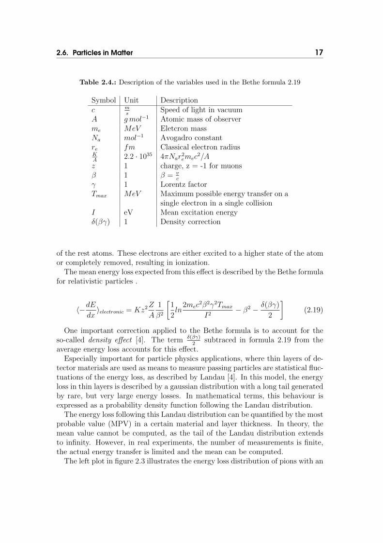
Table 2.4.: Description of the variables used in the Bethe formula 2.19
Symbol Unit Descriptionc m
sSpeed of light in vacuum
A gmol−1 Atomic mass of observerme MeV Eletcron massNa mol−1 Avogadro constantre fm Classical electron radiusKA
2.2 · 1035 4πNar2emec
2/Az 1 charge, z = -1 for muonsβ 1 β = v
c
γ 1 Lorentz factorTmax MeV Maximum possible energy transfer on a
single electron in a single collisionI eV Mean excitation energyδ(βγ) 1 Density correction
of the rest atoms. These electrons are either excited to a higher state of the atomor completely removed, resulting in ionization.
The mean energy loss expected from this effect is described by the Bethe formulafor relativistic particles .
〈−dEdx〉electronic = Kz2
Z
A
1
β2
[1
2ln
2mec2β2γ2TmaxI2
− β2 − δ(βγ)
2
](2.19)
One important correction applied to the Bethe formula is to account for theso-called density effect [4]. The term δ(βγ)
2subtraced in formula 2.19 from the
average energy loss accounts for this effect.Especially important for particle physics applications, where thin layers of de-
tector materials are used as means to measure passing particles are statistical fluc-tuations of the energy loss, as described by Landau [4]. In this model, the energyloss in thin layers is described by a gaussian distribution with a long tail generatedby rare, but very large energy losses. In mathematical terms, this behaviour isexpressed as a probability density function following the Landau distribution.
The energy loss following this Landau distribution can be quantified by the mostprobable value (MPV) in a certain material and layer thickness. In theory, themean value cannot be computed, as the tail of the Landau distribution extendsto infinity. However, in real experiments, the number of measurements is finite,the actual energy transfer is limited and the mean can be computed.
The left plot in figure 2.3 illustrates the energy loss distribution of pions with an
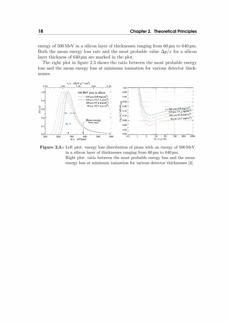
18 Chapter 2. Theoretical Principles
energy of 500 MeV in a silicon layer of thicknesses ranging from 60 µm to 640 µm.Both the mean energy loss rate and the most probable value ∆p/x for a siliconlayer thickness of 640 µm are marked in the plot.
The right plot in figure 2.3 shows the ratio between the most probable energyloss and the mean energy loss at minimum ionization for various detector thick-nesses.
Figure 2.3.: Left plot: energy loss distribution of pions with an energy of 500 MeVin a silicon layer of thicknesses ranging from 60 µm to 640 µm.Right plot: ratio between the most probable energy loss and the meanenergy loss at minimum ionization for various detector thicknesses [4].

Chapter 3The Large Hadron Collider
CERN is the European organization for nuclear research and has been establishedin 1954 to promote peaceful research in the field of nuclear physics among its mem-ber states. In 2014, 20 countries located on the European continent are memberstates of CERN. The total number of CERN member states is 21, with Israeljoining CERN in 2013 as a full member state. Other countries hold an observerstatus, for example the United States of America and the Russian Federation, andare involved in experimental work at CERN, as well.
The Large Hadron Collider (LHC) [3] [11] is a particle accelerator complexwhich is located at CERN near Geneva and spans across the French and Suisseborder.
The LHC accelerates two beams of protons in opposite directions along theaccelerator ring and focuses these beams on to each other in the so-called inter-action points. In its previous operational phases, the LHC was running with acenter-of-mass energy of
√s = 7 TeV and
√s = 8 TeV and will be increased to the
design value of√s = 14 TeV in the coming years. Already with these energies,
the LHC machine passed all previous collider experiments in terms of the maxi-mally achieved center-of-mass energy. Before the LHC, the Tevatron [13] proton-antiproton collider at the Fermi National Accelerator Laboratory near Chicagoachieved the highest center-of-mass energy with
√s= 1.96 TeV.
The Large Electron-Positron Collider(LEP) [14] was operated from 1989 to 2000at CERN and the machine and the scientific team provided many important sci-entific contributions. One of the most prominent is the measurement of the Zboson mass with an unparalleled accuracy [15]. As part of the LEP’s construc-tion, a 26.7 km long underground tunnel was excavated in a depth ranging from56m to 170m. This tunnel was reused for the LHC once the LEP collider wasdecommissioned in 2000.
One important feature of the LHC design is to employ superconducting magnetsoperated at a temperature below 2 K which can generate a magnetic field of up
19

20 Chapter 3. The Large Hadron Collider
Figure 3.1.: Schematic of the LHC accelerator complex with the four main experi-ments and the PS and SPS pre-accelerators. Taken from [12].
to 8 T. Such a strong field is necessary to hold the beam of charged particles ontheir circular path.
Before protons are injected into the 26.7 km long LHC accelerator itself, theyare pre-accelerated by a set of smaller accelerators. By using this technique, theprotons are injected into the LHC with an energy of 450 GeV and are furtheraccelerated using radio frequency cavities to their final energy. Furthermore, theLHC accelerator complex has been designed to also allow the acceleration of heavyions, in particular lead ions. In place of protons, they can also to be injected,accelerated and collided inside the LHC machine.
The LHC machine provides beam collisions at four interaction points, wherethese experiments are located:
• Compact Muon Solenoid (CMS) This machine was built as a general-purpose detector for a wide variety of physics studies, among others thesearch for possible Higgs particles.
• A Large Ion Collider Experiment(ALICE) This detector was specifi-cally desgined to record the collisions during the heavy ion operation modeof the LHC.
• A Toroidal LHC ApparatuS (ATLAS) Similar to CMS, ATLAS wasdesgined as a general-purpose machine with a broad physics programme.

3.1. Scientific Goals 21
• Large Hadron Collider beauty (LHCb) This machine is optimized tocover the forward region of particle collisions and focuses of the measurementof b-mesons and their decays.
The particle beams in the LHC machine are not continuous, but subdividedin so-called bunches. The minimum time between the collision of these bunchesinside the four experiments is 25 ns in the current LHC design.
3.1. Scientific Goals
The scientific program of the LHC and its experiments is very ambitious and spansa wide range of open and current questions in particle physics and cosmology. Inthe following, some of the major fields of interest will be outlined.
3.1.1. Higgs Boson
The standard model Higgs boson was postulated in 1964 by independent groupsof scientists [16] [17] as part of the Higgs mechanism which is responsible forgiving mass to other elementary particles.
The four collaborations at the LEP experiments combined their measurementdata and were able to establish a lower bound of 114.4 GeV/c2, at the 95% confi-dence level, on the mass of the Standard Model Higgs boson [18].
One important research goal of the LHC and its experiments is the search for theHiggs boson in a wide mass range and, if found, the examination of its properties.
In July 2012, both the CMS and ATLAS experiments announced the discov-ery of a new particle which is compatible with the standard model Higgs bo-son [19][20]. The CMS experiment reported a mass of 125.3 ± 0.4 (stat) ±0.5 (syst) GeV and the ATLAS experiment published their results with a mass of126.0 ± 0.4 (stat) ± 0.4 (syst) GeV.
In the upcoming LHC run period, this new particle will be further studied andits parameters like spin will be measured in detail.
3.1.2. Quark-Gluon-Plasma
The Quark-Gluon-Plasma (QCP) is a proposed state of matter, in which theconfinement of quarks and gluons is non-existent, due to the high temperature.Running the LHC in the lead ion mode, allows to create high enough temperaturesto potentially recreate the QCP state and therefore study its properties directly.
22 Chapter 3. The Large Hadron Collider
3.1.3. Precision Measurement of the Standard ModelThe standard model of particle physics is incredibly successful in describing theprocesses in the energy ranges which have been probed so far.
With the new energy range provided by the LHC machine, the predictions madeby the standard model can be tested in this areas and the free parameters of themodel can be adapted to this new energy range.
3.1.4. CP ViolationThe LHCb experiment has been specifically designed to study the CP violationto help understand the matter-antimatter asymmetry we observe in the universetoday. Six key measurements of B-decays have been selected to be performed atthe LHCb experiment [21].
3.1.5. Physics Beyond the Standard ModelObserved phenomena, like the dark matter and dark energy content of the uni-verse, cannot be easily explained with the elementary particles contained in thestandard model.
One theoretical class of models are the supersymmetric extensions, in whicheach elementary particle from the standard model gets assigned a superpartner.The LHC experiments look for signatures of these SUSY particles, mostly byanalysing the missing transverse energy ( ~E/T ) of events.
3.2. LHC Machine ParametersAs outlined in the previous theory chapter, the luminosity is an important prop-erty of a particle collider. The number of observed collisions is
Nevents = L · σevent (3.1)
here L is the luminosity of the collider and σevent is the cross section of a specificphysics process. Under the assumption of a Gaussian beam distribution, theluminosity L of the LHC can be calculated using:
L =N2b k frev γr4πεnβ?
F (3.2)
wherein Nb is the number of particles per bunch, k is the number of overall bunchesin the machine, frev is the revolution frequency of the beam, γr is the relativisticgamma factor, εn the normalized transverse beam emittance and β? the beta func-tion at the collision point. F is a geometric luminosity reduction factor necessarydue to deviation from π of the crossing angle at the interaction point.

3.2. LHC Machine Parameters 23
1 Apr1 M
ay1 Ju
n1 Ju
l1 Aug
1 Sep1 O
ct1 N
ov1 D
ec
Date (UTC)
0
5
10
15
20
25
Tota
l In
teg
rate
d L
um
inosit
y (fb¡1)
£ 100
Data included from 2010-03-30 11:21 to 2012-12-16 20:49 UTC
2010, 7 TeV, 44.2 pb¡1
2011, 7 TeV, 6.1 fb¡1
2012, 8 TeV, 23.3 fb¡1
0
5
10
15
20
25
CMS Integrated Luminosity, pp
Figure 3.2.: The integrated luminosity delivered to CMS by the LHC machine in theyears 2010, 2011, 2012. The graphs shown here are for proton-protoncollisions only. Taken from [22].
The specified luminosity for proton-proton operation mode for the ATLAS andCMS experiments is L = 1034cm−2s−1 [23]. As outlined in the theory chapter,such a large luminosity is required to also be able to study rare processes whichhave a very small cross section. At the design luminosity of the LHC machine,around 20 inelastic events occur at the same time as the physics process of interest.This large background poses a significant challenge to both the detector hardwareand software systems.
Table 3.1.: Machine parameters for the LHC [24][25] and the proposed HL-LHCmachine [26].
Parameter LHC Run 2012 (at CMS) HL-LHC (est.)Peak L [cm−2s−1 ] 7.9 · 1033 2.2 · 1035
Integrated L [fb−1] 23.3 3000√s [TeV] 8 14
number of bunches [1] up to 1400 2808bunch spacing [ns] 50 25β∗[m] 0.6 0.15

24 Chapter 3. The Large Hadron Collider
1 Jun
1 Sep1 D
ec1 M
ar1 Ju
n1 Sep
1 Dec
1 Mar
1 Jun
1 Sep1 D
ec
Date (UTC)
0
2
4
6
8
10
Peak D
elivere
d L
um
inosit
y (Hz=nb)
£ 10
Data included from 2010-03-30 11:21 to 2012-12-16 20:49 UTC
2010, 7 TeV, max. 203.8 Hz=¹b2011, 7 TeV, max. 4.0 Hz=nb2012, 8 TeV, max. 7.7 Hz=nb
0
2
4
6
8
10
CMS Peak Luminosity Per Day, pp
Figure 3.3.: The peak luminosity per day delivered to CMS by the LHC machinein the years 2010, 2011, 2012. The graphs shown here are for proton-proton collisions only. Taken from [22].
3.3. Possible Scenarios for an LHC UpgradeWhile the LHC machine is still in operation, studies are already under way forpossible machines to follow up on the discoveries made by the LHC. One of themost prominent proposals is the High Luminosity LHC (HL-LHC) [26]. At thecore of this proposal is an upgrade to the current LHC machine over the nextyears leading to an HL-LHC by the year 2020. The design proposes to increasethe collision data that can be recorded per year to 250fb−1 which leads to anaccumulated amount of 3000fb−1 for an estimated 12 years of operation [26]. In itscurrent design state, the proposed machine will be able to deliver 2.2∗1034cm−2s−1
of peak luminosity which is 10 times more then the current LHC is capable of.The plan is to achieve this increase in luminosity by using a strong focus schemeto reach very low values of the β function at the collision points [26].
With this increased luminosity, the HI-LHC will be able to increase the mea-surement accuracy on the properties of particles discovered at the LHC. It willfurthermore allow to observe very rare processes which can not be accessed by theLHC, due to its smaller luminosity.

Chapter 4CMS Experiment
More than 3000 scientist and engineers from 38 countries form the CMS Col-laboration and have designed, built and are operating the CMS detector at theLHC accelerator complex. During the design phase of the CMS detector, a set ofrequirements were defined to guide the development process [23]:
• Muon Reconstruction Good muon identification and a di-muon massresolution of ≈ 1% at a muon energy of 100 GeV.
• Charged-particle momentum resolution Design of a tracking systemwhich is able to distinguish particle trajectories close to the interaction point.
• Electromagnetic Resolution An electro-magnetic calorimeter which isable to achieve a di-photon and di-electron mass resolution of ≈ 1% at anparticle energy of 100 GeV.
• Missing Transverse Energy Measurement The E/T measurement is animportant experimental method to spot possible new physics processes.Therefore, the detector should be as hermetic as possible to enable E/T mea-surements.
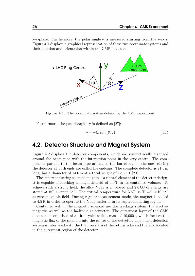
4.1. Coordinate SystemThe Cartesian coordinate system definition used within the CMS Collaborationplaces the origin at the beam interaction point, which is at the very center of theCMS detector. Furthermore, the x-axis is defined to point at the center of theLHC accelerator ring and the y-axis points upwards. Finally, the z-axis is orientedalong the beam pipe in the direction of the Jura mountain range.
To take advantage of the symmetrical nature around z-axis, also a polar coordi-nate system can be defined. The azimuthal angle Φ starts from the x-axis in the
25
26 Chapter 4. CMS Experiment
x-y-plane. Furthermore, the polar angle θ is measured starting from the z-axis.Figure 4.1 displays a graphical representation of these two coordinate systems andtheir location and orientation within the CMS detector.
LHC Ring Centre
Φ Θ
beam pipe
Juramountains
zx
y
Figure 4.1.: The coordinate system defined by the CMS experiment.
Furthermore, the pseudorapidity is defined as [27]:
η = −ln tan (θ/2) (4.1)
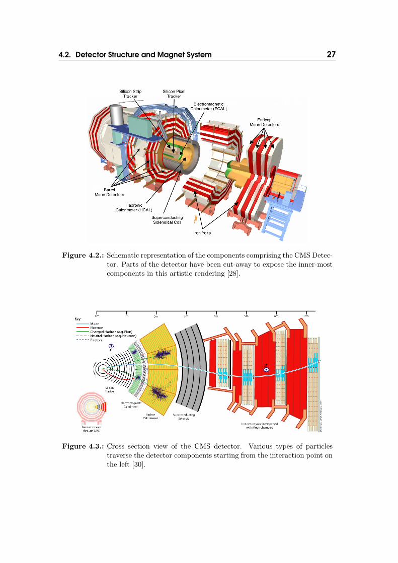
4.2. Detector Structure and Magnet SystemFigure 4.2 displays the detector components, which are symmetrically arrangedaround the beam pipe with the interaction point in the very centre. The com-ponents parallel to the beam pipe are called the barrel region, the ones closingthe detector at both ends are called the endcaps. The complete detector is 21.6 mlong, has a diameter of 14.6 m at a total weight of 12,500 t [29].
The superconducting solenoid magnet is a central element of the detector design.It is capable of reaching a magnetic field of 4.0 T in its contained volume. Toachieve such a strong field, the alloy NbTi is employed and 2.6 GJ of energy arestored at full current [29]. The critical temperature for NbTi is Tc = 9.25 K [29]at zero magnetic field. During regular measurement mode, the magnet is cooledto 4.5 K in order to operate the NbTi material in its superconducting regime.
Contained within the magnetic solenoid are the tracking system, the electro-magnetic as well as the hadronic calorimeter. The outermost layer of the CMSdetector is comprised of an iron yoke with a mass of 10,000 t, which focuses themagnetic flux of the solenoid into the center of the detector. The muon detectionsystem is interlaced with the the iron slabs of the return yoke and therefor locatedin the outermost region of the detector.
4.2. Detector Structure and Magnet System 27
Figure 4.2.: Schematic representation of the components comprising the CMS Detec-tor. Parts of the detector have been cut-away to expose the inner-mostcomponents in this artistic rendering [28].
Figure 4.3.: Cross section view of the CMS detector. Various types of particlestraverse the detector components starting from the interaction point onthe left [30].

28 Chapter 4. CMS Experiment
4.3. Inner Tracking SystemThe tracking system, located at the inner-most part of the CMS detector, isessential to detect and reconstruct trajectories of charged particles close to theinteraction point. The entire tracking system is based on silicon technology andhas an overall length of 5.8 m and a diameter of 2.5 m.
Closest to the interaction point are three layers of silicon pixel detectors in thebarrel and two layers in the endcap region. The high position resolution providedby pixel detectors is required to be able to separate the many particles originatingat the interaction point. In total, the pixel detector elements cover an area ofabout 1 m2 and have 66 million pixels combined.
Following the pixel elements, are 10 layer of silicon strip detector elements inthe barrel and 11 layers in the endcap region. Using this approach, the trackingsystem provides a full coverage in φ and offers a tracker acceptance of up to|η| < 2.5.
Chapter 5 will go into more detail on the tracking system’s design, materialbudget and operational performance.
4.4. Electromagnetic CalorimeterThe detector component directly following the tracking system is the electromag-netic calorimeter (ECAL) which is made up of lead tungstate (PbWO4) crystals.In total, 61 200 crystals are integrated into the barrel region and 7 324 crystalsare located in each of the two endcap regions [29]. One advantage of the PbWO4-crystals is that about 80% of all scintillation photons are emitted within the 25 nsbunch crossing time of the LHC machine [29].
The ECAL systems covers the whole φ range. Furthermore, the barrel sectionof the ECAL (named EB) extends over the pseudorapidity range of |η| < 1.479while the endcap ECAL (named EE) extends from 1.479 < |η| < 3.0.
Two different types of read-out systems are used for the barrel and endcapregions of the ECAL due to the different radiation profiles and magnetic fieldsetups. The barrel region ECAL uses avalanche photodiodes while the endcapregion uses vacuum phototriodes.
4.5. Hadronic CalorimeterAs displayed in figure 4.4, the hadronic calorimeter of the CMS experiment isconstituted by four individual elements. The barrel HCAL (named HB) is locatedin the central region of the CMS detector and covers an region of up to |η| < 1.3while the two endcap HCALs (named HE) are located at both ends of the detectorand cover the range of 1.3 < |η| < 3.0 [29]. Both the HB and HE parts of

4.6. Muon System 29
the hadronic calorimeter are fully located within the 4 T strong magnetic fieldgenerated by the solenoid magnet.
Located outside of the magnetic solenoid, the outer hadronic calorimiter (namedHO) is installed in the central region of the CMS detector and covers the regionof |η| < 1.3. Its purpose is to measure particles which have not been fully stoppedwithin the electromagnetic EB and hadronic calorimeter HB in the barrel region.
The hadronic calorimeter setup is completed by the forward HCAL (namedHF). It is located in the forward region of the detector, 11.2 m away from theinteraction point and extends the calorimeter coverage to |η| = 5.2.
Figure 4.4.: The location of the four elements constituting the hadronic calorimeterof the CMS detector. The muon system is highlited in purple [23].
The design of the hadronic calorimeter in the barrel region will be showcasedin the following. It is constituted of brass plates with a thickness of 50.5 mmwhich are interlaced with plastic scintillator material with a thickness of 3.7 mm.Photons, which are emitted in the scintillating material, are sampled with wave-length shifting fibers and are guided to hybrid photodiodes where a correspondingelectronic signal is generated.
4.6. Muon SystemThis sub-system of the CMS detector provides high-precision measurements ofmuon tracks. In order to facilitate this, the muon system must identify particlesas muons and perform a precise measurement of their charge and momentum.

30 Chapter 4. CMS Experiment
The muon system of CMS covers an overall area of 25 000 m2 [29] and is thereforthe detector element with the largest area within the CMS detector. It is installedin between the iron slabs of the magnetic return yoke and uses drift tube tech-nology in the central barrel region to cover the area of |η| < 1.2. A gas mixtureconstituted of 85% Ar and 15% CO2 is contained within the tubes and in total172 000 sensing wires are installed to detect the ionization of the gas mixture bypassing high-energetic particles.
In contrast, the two endcap regions use cathode strip chambers (CSC) technol-ogy to detect passing particles. This part of the muon detection system coversthe region of 0.9 < |η| < 2.4.
4.7. Trigger SystemThe LHC machine achieves a beam crossing every 25ns, which results in a crossingfrequency of 40 MHz [29]. At this high rate, it becomes technically impossible tostore all collision information with a justifiable amount of resources. Therefore,a data reduction scheme needs to be adopted which filters undesired events andreduces the storage size of interesting events. These events are stored to disk andcan be processed and analyzed in more detail later.
Level-1 Trigger
The CMS collaboration opted to install multiple levels of triggers to achieve adata reduction along the various stages of the trigger. The first stage is theLevel-1 trigger system which is located close to the actual detector. This logic isimplemented on custom electronic boards which link directly to trigger systemsin the tracker, calorimeter and muon system hardware. These systems can flag ameasured event, for example if a certain threshold energy was exceeded or a muonwas identified. The trigger decisions of all sub-detectors are reported back to thecentral trigger system which then discards the event or passes it on to the HighLevel Trigger (HLT) for further evaluation.
Using this technique, the Level-1 trigger can achieve a reduction of the eventrate from 40 MHz to 100 kHz. In this process, around 99.75 % of all measuredevents are excluded from further processing [23].
High Level Trigger System
All events which have been accepted by the Level-1 trigger system are forwardedto the High Level Trigger (HLT). For the first time, all data gathered by the var-ious sub-detectors is combined to achieve a complete picture of the event. Thisallows to reconstruct the trajectory, momentum and charge of particles travers-ing the detector. Fine-grained trigger decisions can now be performed using the

4.7. Trigger System 31
information available to the HLT. A comprehensive list of trigger criteria, namedTrigger Paths [31], is compiled by the teams of physicists interested in a specificevent topology. For example, a trigger criteria can be defined which stores theevent only if at least two muons have been reconstructed with sufficient quality.Another Trigger Path can be configured to store events which contain a tau decaycandidate.
Furthermore, a pre-scale value can be assigned to each Trigger Path. Usingthese technique, only a fraction (defined by the pre-scale value) of all triggeredevents is actually stored on disk, while the rest is discarded. This allows to reducethe necessary data rate of Trigger Paths which have a high acceptance rate andstill retain the possibility to study these types on events later.
The HLT-logic is implemented as a computing farm comprised of 10.000 com-modity server x86 CPUs. The necessary event reconstruction is a software ap-plication running in a highly-distributed fashion on these machines. Therein, thesame or very similar algorithms are used as in the offline event reconstruction,which is described in more detail in the chapters 6 and 7. This allows for a flex-ible setup of the HLT and improvements in the event reconstruction algorithmsalso benefit the online event selection.
During the 2012 run, the HLT was configured to achieve an output frequencyof 300 Hz while the input stream of events was provided by the level-1 trigger at arate of 100 kHz. All events accepted by the HLT system are transferred from theCMS Detector’s location at Point 5 to CERN’s central data center and stored forlater offline reconstruction.


Chapter 5CMS Tracker
Robust and reliable track and vertex reconstruction play an important role inthe high-luminosity environment provided by the LHC machine. Achieving agood particle identification and measurement resolution with more than 20 pileup collisions overlaying the actual primary one is a challenge to be addressed bythe tracker hardware design and reconstruction software.
This chapter will outline the hardware design of the tracking system whilechapter 7 will detail the track reconstruction algorithms.
5.1. Design Goals of the Tracking System
5.1.1. Momentum Resolution
The decay of the W and Z gauge boson plays an important role in the processesobserved at the LHC machine. Especially their decays into leptons provide cleansignals for analysis [32]. Therefore, the tracker must provide a good momentumresolution in a wide momentum range to infer the energy carried by the theseparticles.
5.1.2. Isolation of Particles
The detection of isolated leptons in the tracker, in particular electrons, playsan important role in assigning energy clusters measured in the electromagneticcalorimeter to decay vertices. This allows to suppress background and helps tomeasure decays like H → ZZ → 4l± in a cleaner way.[32]
To achieve this, an effective reconstruction of all tracks down to 1 GeV isnecessary.[32]
33

34 Chapter 5. CMS Tracker
5.1.3. B-tagging Abilities
The ability to reconstruct and identify jets resulting from a beauty quark decayis very important, as they are considered important signals for new physics, canhelp to give more insight into the CP violation and are an essential tag for topquark physics [32].
To be able to achieve this, the decay vertex must be identified properly and lowpT tracks must be correctly reconstructed and assigned.
5.1.4. Vertexing and Decay Chains
With around 20 pile-up interactions overlaying the primary collision, a reliable andefficient vertex reconstruction must be deployed. It is responsible for detectingcollision points (vertices) and assigning reconstructed tracks to them. As thevertices are located inside the high-vacuum beam line, they can not be measureddirectly, but can only be inferred from the reconstructed tracks.
Therefore, the track resolution close to the collision area must be high enoughto allow for a reliable vertex reconstruction and track assignment.
Furthermore, particle decay in flight within the tracking detector must be de-tected, resulting tracks reconstructed and properly assigned to the decay location.These locations are named secondary vertices.
Secondary vertex reconstruction is essential for observing the decay of the short-lived Kaon K0
s which will be described in chapter 7.7.
5.1.5. High Particle Multiplicities
The LHC offers the unique possibility to also produce high-energetic heavy ioncollisions and can potentially produce a Quark-Gluon-Plasma. These events arealso recorded by CMS and have a very high multiplicity of up to 25,000 parti-cles [32] and the tracking system has to be able to cope and operate in such ahigh-occupancy environment.
5.2. Measurement Principle
The physical principal behind Silicion-based tracking systems is that of semi-conductivity. In terms of their electrical conductivity, different type of mattercan be separated into the three classes conductors, semi-conductors and isolators.The property which allows this separation is the so-called bandgap Eg betweenthe conduction band and the valence band. The band-gap can be computed asfollows:
Eg = Ec − Ev

5.2. Measurement Principle 35
Ev is the highest possible electron energy state in the valence band and Ec thelowest possible electron energy state in the conduction band.
While the valence band electrons are bound to their corresponding atoms, in theconduction band they are loose and can move quasi-free in the material. Metals areconductors because they have no band-gap and only very little energy is requiredto allow for electrons to move freely in the lattice structure of the metal. On theother hand, with insulators, the band gap is significant and the energy necessaryto excite electrons to move from valence band to the conduction band is high.
Semi-conductors are localised between these two poles and are defined as havinga significant band-gap energy, but still smaller then Eg < 5eV .For example, thebandgap of Silicon at room temperature is Eg = 1.11eV [33].
This results in semi-conductors being isolators if their electrons are all in thelowest possible energy state. Only very little is energy is necessary to move elec-trons into the conduction band and make them act as quasi-metals. This ex-traordinary property of semi-conductors allows to use them in a wide range ofapplications from transistors in electronics, digital cameras to HEP tracking sys-tems.
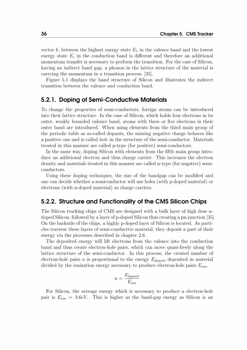
Figure 5.1.: Band structure of Silicon. The band gap region is marked with a greybackground. Own work based on [34].
The transition between the valence and conduction bands can be separated intotwo types. In a direct band gap, only energy needs to be transferred in order tobridge the gap. The momentum between the two states is equal and needs not tobe changed. In an indirect band gap, the crystal momentum, defined by the wave
36 Chapter 5. CMS Tracker
vector k, between the highest energy state Ev in the valence band and the lowestenergy state Ec in the conduction band is different and therefore an additionalmomentum transfer is necessary to perform the transition. For the case of Silicon,having an indirect band gap, a phonon in the lattice structure of the material iscarrying the momentum in a transition process. [35].
Figure 5.1 displays the band structure of Silicon and illustrates the indirecttransition between the valence and conduction band.
5.2.1. Doping of Semi-Conductive MaterialsTo change the properties of semi-conductors, foreign atoms can be introducedinto their lattice structure. In the case of Silicon, which holds four electrons in itsouter, weakly bounded valence band, atoms with three or five electrons in theirouter band are introduced. When using elements from the third main group ofthe periodic table as so-called dopants, the missing negative charge behaves likea positive one and is called hole in the structure of the semi-conductor. Materialstreated in this manner are called p-type (for positive) semi-conductors.
In the same way, doping Silicon with elements from the fifth main group intro-duce an additional electron and thus charge carrier. This increases the electrondensity and materials treated in this manner are called n-type (for negative) semi-conductors.
Using these doping techniques, the size of the bandgap can be modified andone can decide whether a semiconductor will use holes (with p-doped material) orelectrons (with n-doped material) as charge carriers.
5.2.2. Structure and Functionality of the CMS Silicon ChipsThe Silicon tracking chips of CMS are designed with a bulk layer of high dose n-doped Silicon, followed by a layer of p-doped Silicon thus creating a pn-junction [35].On the backside of the chips, a highly p-doped layer of Silicon is located. As parti-cles traverse these layers of semi-conductive material, they deposit a part of theirenergy via the processes described in chapter 2.6.
The deposited energy will lift electrons from the valence into the conductionband and thus create electron-hole pairs, which can move quasi-freely along thelattice structure of the semi-conductor. In this process, the created number ofelectron-hole pairs n is proportional to the energy Edeposit deposited in materialdivided by the ionization energy necessary to produce electron-hole pairs Eion.
n =EdepositEion
For Silicon, the average energy which is necessary to produce a electron-holepair is Eion = 3.6eV. This is higher as the band-gap energy as Silicon is an

5.2. Measurement Principle 37
Figure 5.2.: Schematic view of the doped Silicon layer used in a CMS Trackerchip [32].
indirect semi-conductor, as part of the energy is necessary to produce a phononin the lattice structure of the material [35].
5.2.3. Bias Voltage and Signal Read-Out
Without any external electric field, the electron-hole pairs created by either ther-mal effects or passing particles vanish in a process of recombination and the sep-aration of positive and negative charges in the semiconductor arrive again at astate of equilibrium [35].
In order to read-out the number of created electron-hole pairs, a so-called biasvoltage [32] is applied to the pn-junction. This voltage will prevent the electron-hole pairs from recombining and allows to collect and count the electrons on then-type side of the chip.
Depending on the type of chip, either a one-dimensional array for strip chipsor a two-dimensional array for pixel chips collects the electrons. This electronicis called chip read-out and can either provide an analog or digital signal to theDAQ system.
The digital read-out type provides a binary signal which is false by default, butis switched to true if the collected amount of charge for one read-out channel islarger then a pre-configured threshold.
The CMS read-out electronics provides an analog readout to the DAQ. Therein,the integer number provided is proportional to the collected charge. As a particlepassing through the Silicon chip leaves a signal for more then one channel, theanalog signal allows for a more detailed determination of the intersection pointbetween the particle trajectory and the detector element surface.

38 Chapter 5. CMS Tracker
5.2.4. Momentum Measurement
While the direction of a particle can be directly measured using the energy de-posits, so-called hits, in the Silicon detectors, the momentum must be derivedindirectly.
As the whole CMS Tracker is embedded in the 3.8 T strong magnetic fieldproduced by the CMS magnet, all charged particles are affected by the Lorentzforce. Assuming there is no electric field, this force can be written as [36]:
~FL = q~v × ~B
Here, q is the charge of the particle, ~B is the strength of the magnetic field andm is the mass of the particle.
As the magnetic field of CMS is oriented along the z direction, the particle trackswill describe a helix along the z direction [36]. Only the transverse componentpT of the particle trajectory is affected by the magnetic field. By determiningthe radius R of the helix, the transverse momentum pT can be derived. Thisis done by the track reconstruction software by using consecutive tracker hits todetermine pT. Furthermore, also the overall momentum can be reconstructedby combining the pT component of the particle momentum and the knowledgeabout the direction of the particle. This procedure is described in more detail insection 7.5.
5.3. Tracker Components
The tracker system is made up by 16588 individual detector elements [37] whichconsist of a Silicon sensor, read-out electronics and energy supply.
These parts are organized in stacked layers in the barrel and endcap region inorder to cover all the required areas.
The tracking system can be separated into two main components. Althoughthese components have a lot in common, like the general measurement principle,and share some of the infrastructure components like energy supply and cooling,they offer different performance in terms of measurement resolution and volumethey cover.
The innermost three barrel detection layers and the first two layers in the endcapregion consist of 1440 Silicon-based detection elements and are able to provide atwo-dimensional measurement of the traversing particle by using a 2d-grid of pixelcells. All of these measurement layers are referred to as the Pixel Tracker.
The remaining layers in the barrel endcap region are populated by 15148 ele-ments of Silicon-based strip detectors. These elements can provide a one dimen-sional hit position perpendicular to their strip direction.

5.3. Tracker Components 39
Figure 5.3.: Photo of a pixel module [38].
Figure 5.4.: R-Z view of one quarter of the CMS Tracker showing pixel and stripsilicon layers. Double sided strip modules are highlighted with thicklines [39].

40 Chapter 5. CMS Tracker
In the R-Z view of the Tracker in Figure 5.4, one can see how the pixel andstrip elements have been arranged in order to cover the range of up to |η| ≤ 2.5.Furthermore, the detector elements cover the full φ space.
5.3.1. Inner Pixel Tracker
Figure 5.5.: Schematic view of the pixel-based inner tracking system. The centralthree layers of barrel modules (green) are visible and the two endcappixel layers (red), which exhibit a fan-like structure, are visible on bothends [38].
The three layers of the barrel pixel system are placed at a mean distance of4.4, 7.3 and 10.2 cm from the primary interaction vertex [38] and are thereforethe closest detector elements to the collision point. The pixel endcap elementsare arranged in two layers in a fan-like structure on both ends of the barrel pixellayers. They are 6 to 15 cm in radius, and are located with a distance of ±34.5 cmand ±46.5 cm from the primary interaction point. Figure 5.5 shows a schematicview of the pixel tracker and highlights the barrel part in green and the endcappart in red.
As these pixel modules are the closest detection modules to the interactionpoint, they have to cope with a high particle rate and still need to be able toprovide sufficient resolution to perform vertex recontstruction and b-tagging in areliable way.
For this reason, these silicon detectors have the highest resolution of the trackingsystem with an individual pixel size of 100 ·150µm2. However, this resolution canbe greatly improved by measuring the charge deposit as an analog value. Bycombining multiple charge distribution across all pixels a particle passed, the

5.4. Material Budget 41
resolution can be greatly improved to ≈ 10µm, . The algorithm used here will bedescribed in detail in chapter 7.
5.3.2. Outer Strip Tracker
The strip part of the tracking system can be further separated into the TIB(Tracker Inner Barrel) and TOB (Track Outer Barrel) components for the barrelregion and into the TID (Tracker Inner Disc) and the TEC (Tracker End Cap)components for the endcap region. This naming scheme is best illustrated byfigure 5.4.
The TIB is made up by four layers with a minimum strip size of 10cm · 80µmand the first two layers are stereo layers, with two strip elements very close to eachother. Having stereo layers allows to combine the two individual strip measure-ments of a single passing particle and derive a two dimensional hit. This enables abetter measurement of the r−φ and z components of the track. Furthermore, byhaving these precise hit informations, stereo layers can also be used to search forsecondary vertices and conversion finding. This will be explained in more detailin chapter 7 which is dedicated to track reconstruction .
Due to the significant drop in occupancy in the outer layers of the tracker, theseven layers of the TOB were designed with a maximum strip size of 25cm · 180µm.Again, the first two layers of the TOB are equipped with stereo modules.
The TID is comprised of three radial discs which fill the gap between the TIBand the TEC. The lower two rings of the TID sensors are stereo modules, too.
The largest part of the tracker endcap region is filled by the nine radial discsof the TEC. As visible in figure 5.4, selected rings of the TEC discs are equippedwith stereo modules, too.
5.4. Material Budget
The so-called material budget is an important quantity in every detector designand refers to the amount and type of matter which incoming particles have to crosswhile inside the detector volume. Sensitive measurement elements in a detectorare denoted active material and are, in the case of a Silicon-based tracking systemthe Silicon sensors. They can be read out to determine the charge deposited by apassing particle. Support structures, cooling, cabling and even air and other gasmixtures are denoted as passive material, as energy deposited in these materialscan not be measured.
Whether a significant amount of active and passive material is favourable de-pends on the detector design and the particles which should be measured. Forexample, the design of the CMS hadronic calorimeter, described in section 4.5,utilizes a big amount of brass plates as passive material. They cause interactions

42 Chapter 5. CMS Tracker
Component Category Mass [kg] Fraction [%]Carbon Fiber 1144.5 27.6Copper and copper alloys 644.5 15.6Aluminium 595.0 14.4Organic materials 472.1 11.4Coolant (C 6 F 14 ) 258.9 6.3Silicon active 225.8 5.5Fiber-glass laminated 213.4 5.2Other mechanical structures 191.7 4.6Inorganic oxides 153.2 3.7Other metals 141.9 3.4Glues and resins 75.3 1.8Electronic component 25.7 0.6
Table 5.1.: Mass distribution across various types of material extracted from theGEANT4 detector model of the CMS Tracker. [37].
with the incoming particles to enable the measurement of resulting secondaryparticles in the active material behind each brass plate.
As described in section 5.2, the CMS tracker was build to measure the energyand direction of passing particles via their curvature in the magnetic field. At thesame time, particles like electrons, charged and uncharged hadrons should passthe tracker without much energy loss, so their energy can be determined in theelectromagnetic and hadronic calorimeters.
To facilitate this, the CMS tracking system was built with very light materialslike carbon fibre composite as support structures. Table 5.1 lists the mass distri-bution derived from the tracker geometry as modelled in the GEANT4 softwarepackage. The estimated total mass of the Tracker amounts to about 4150 kg [37]distributed within a total tracker volume of about 23.5m3.
One can see from table 5.1, that the active Silicon material amounts to around5% of the overall mass of the tracking system.
Furthermore, the mass of active and passive material is concentrated at thedetector layers, their support structures, cooling and wiring. Figure 5.6 shows themass distribution in radiation length for the each tracker subcomponent and forthe pixel tracker only. Both plots have been generated from the tracker geometrymodelled in the GEANT4 software package. The active measurement area of thetracking system is limited to |η| ≤ 2.5 and material plotted above |η| > 2.5 willnot affect the track measurements, but detectors further away from the interactionpoint (for example the forward hadronic calorimeter (HF)).
The left plot illustrates that the lowest radiation length x/X0 in the design ofthe tracker is in the central part η ≈ 0 while the largest are located at around
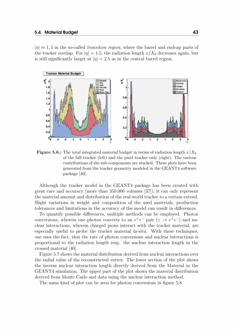
5.4. Material Budget 43
|η| ≈ 1, 5 in the so-called transition region, where the barrel and endcap parts ofthe tracker overlap. For |η| > 1.5, the radiation length x/X0 decreases again, butis still significantly larger at |η| = 2.5 as in the central barrel region.
Figure 5.6.: The total integrated material budget in terms of radiation length x/X0
of the full tracker (left) and the pixel tracker only (right). The variouscontributions of the sub-components are stacked. These plots have beengenerated from the tracker geometry modeled in the GEANT4 softwarepackage [40].
Although the tracker model in the GEANT4 package has been created withgreat care and accuracy (more than 350.000 volumes [37]), it can only representthe material amount and distribution of the real-world tracker to a certain extend.Slight variations in weight and composition of the used materials, productiontolerances and limitations in the accuracy of the model can result in differences.
To quantify possible differences, multiple methods can be employed. Photonconversions, wherein one photon converts to an e+e− pair (γ → e+e−) and nu-clear interactions, wherein charged pions interact with the tracker material, areespecially useful to probe the tracker material in-situ. With these techniques,one uses the fact, that the rate of photon conversions and nuclear interactions isproportional to the radiation length resp. the nuclear interaction length in thecrossed material [40].
Figure 5.7 shows the material distribution derived from nuclear interactions overthe radial value of the reconstructed vertex. The lower section of the plot showsthe inverse nuclear interaction length directly derived from the Material in theGEANT4 simulation. The upper part of the plot shows the material distributionderived from Monte Carlo and data using the nuclear interaction method.
The same kind of plot can be seen for photon conversions in figure 5.8.

44 Chapter 5. CMS Tracker
Using this technique, the agreement between the GEANT4 model of the trackerand the actual amount and distribution of material in the real-world tracker wasestimated to be in the range of ≈ 10% [40].
Figure 5.7.: Material distribution derived from nuclear interactions plotted over theradial value of the reconstructed conversion vertex. The lower sectionof the plot shows the inverse nuclear interaction length directly derivedfrom the Material in the GEANT4 simulation. The upper part of theplot shows the material distribution derived from Monte Carlo and datausing the nuclear interaction method. Taken from [41].

5.4. Material Budget 45
Figure 5.8.: Material distribution derived from photon conversions plotted over theradial value of the reconstructed conversion vertex. The lower sectionof the plot shows the inverse radiation length directly derived from theMaterial in the GEANT4 simulation. The upper part of the plot showsthe material distribution derived from Monte Carlo and data using thephoton conversion method. Taken from [41].

Chapter 6CMS Software and Computing
To further process and analyze the data delivered by the CMS Detector, a wholerange of software processing steps are necessary. This includes the unpacking ofthe raw data stream from the detector’s read-out electronics, applying calibrationconstants, reconstructing particle trajectories up to selecting events with a specifictopology. The CMS Software Framework, short CMSSW [42], is a C++ appli-cation which is used to implement all these functionalities in a modular manner.It allows to configure the individual modules and define the data and control-flowamong modules. In the following, the main building blocks of the CMS SoftwareFramework will be outlined and examples for specific modules will be given.
6.1. CMS Software FrameworkOne central concept employed by CMSSW is the Event Data Model (EDM) ex-change technique [38]. All raw measurement data and derived products, like re-constructed particle tracks and energy deposits, are stored in a central container.Software modules retrieve their input data from this container and store the resultof their processing back to this container. Data items stored in the container canbe identified either by their data type or name. This concept decreases the depen-dence among the modules to a minimum and allows for a flexible configuration ofthe module execution order.
Modules are arranged in so-called Paths which define the execution order, andtherefore the processing hierarchy, of the setup. Furthermore, multiple Paths canbe defined and filled with equal modules but different configurations. This allowsto process the same set of input data with different configurations, for examplecalibration constants.
47

48 Chapter 6. CMS Software and Computing
It is possible to implement a CMSSW module in one of the following categories:
• Source
Event data can either be read from files or via network streams. In case ofoffline processing, previously stored events are loaded from the disk massstorage system. In the HLT setup, event data is streamed via a networkconnection directly into CMSSW using a special source module.
• Producer
Producer modules read data items from the central data store and add anewly created product, which contains the result of the module’s computa-tion, to the data store. The CMS event reconstruction is implemented asProducer modules which are connected by multiples Paths. One of thesemodules is the track finding step, which loads the tracker hits from the cen-tral store, applies the track finding algorithms and outputs a list of foundtrack candidates to the central data store.
• Filter
In contrast to the Producer, no output data object is created by the Filter.These modules can access all data items produced so far and decide whetherthe execution of a Path is continued or stopped. This allows to quit theprocessing of a event which does not suffice the criteria of the topology ofinterest, for example no two muons were measured.
• Analyzer
The data items created by the Producer module can be read by a specificAnalyzer module. In contrast to the Producer, Analyzer modules don’t savetheir results back to the data store but store them on the disk in the formof data tables, histograms and graphs.
• Output
Output modules store the current content of the data store to the disk. Thesaved file can be later used to restore the state of the data store, continueprocessing or apply further analysis steps.
6.2. ROOT Data Analysis FrameworkMany high-energy physics experiments share the same software requirements interms of data storage, statistical analysis and visualization and plotting needs.The ROOT [43] framework has been developed as a comprehensive software li-brary and application to address these areas. It is maintained by a core develop-ment team mostly located at CERN and used by all major high-energy physics

6.3. Event Simulation 49
experiments today. The largest part of ROOT’s functionalities are implementedusing the C++ language, but also python can be used to create programs usingclasses and functions offered by the ROOT library.
One of ROOT’s most prominent features is its ability to store the contentof C++ classes to disk and load them again at a later stage. Nearly all HEPexperiments use this functionality to save their recorded event data and to store areduced set of values for analysis purposes, so-called n-tuples. Furthermore, due toROOT’s standardized data format, the files created can also be used to exchangedata within one experiment’s working groups or even across experiments.
6.3. Event Simulation
To compare the predictions of various theoretical models with the observed eventsin the CMS Detector, a sophisticated event simulation is employed. Starting withthe proton-proton collision in the beam pipe, a chain of consecutive simulationsteps is performed. The initial collision products resulting from the parton-parton-interaction can be generated by so-called Monte Carlo event generators. Variousgenerators are available including PYTHIA [44], Herwig [45], Alpgen [46], Mad-Graph [47] or Sherpa [48] and many of them can be interfaced by the CMSSWframework.
Using Monte-Carlo based methods, an event generator can compute the finalstate of various physics processes. The decay, propagation and their interactionwith the material of the CMS detector of these particles is simulated via a detectorsimulation step. Energy deposits resulting from these particles are recorded andused as input for the event reconstruction to understand the detector responseand measurement resolution for specific event topologies.
Furthermore, the information of the event generator is retained and can becompared to the result of the event reconstruction. This allows to estimate thereconstruction quality and particle finding efficiency of the hardware and softwareelements of the detector.
6.3.1. Event Generators
Many event generators are in active development and differ in the amount andtype of physics processes they have implemented. Among the most popular arePYTHIA [44], Herwig [45] and Sherpa [48] which can be directly used from withingthe CMSSW framework.
The PYTHIA event generator has been used to produce events for this thesis.Therefore, this software package will be introduced in more depth in the following.It implements more than 300 leading order calculations of physics processes of theStandard Model, Minimal Supersymmetric extension of the Standard Model and

50 Chapter 6. CMS Software and Computing
non-standard physics [44].
A model-based process can be applied to particles subjected to QCD confine-ment to reach a colourless final state. This process is called fragmentation, asthe coloured particles result in a shower of colour neutral particles. By default,PYTHIA uses the Lund model to calculate the final hadronic state of the event.The interaction between partons is modelled by a virtual string which is stretchedas the particles move apart. If a critical tension in the string is reached, it ripsand new particles are produced at the ends of the two new strings. This processis performed until only non-coloured particles are left. This showers of hadronicparticles are not bound by QCD confinement and can freely propagate [11].
Additionally, PYTHIA simulates the decay of the hadronic particles created bythe collision, so only quasi-stable particles are left in the final state [11].
PYTHIA is also able to simulate the underlying event, which consists of multipleparton interaction in the beam pipe and is an important background signal formany investigated physics processes. Also the initial and final state radiation istaken into consideration by the PYTHIA simulation run. The implementationof this features are based on phenomenological models and are depending onthe centre-of-mass-energy used at the detector. So-called Tunes contain a set ofparameters which have been optimised to fit the behaviour observed in actualmeasurements[49] [11].
6.3.2. Detector Simulation
To simulate the interaction of the detector components with passing particles, thegeometrical layout and magnetic field of the CMS detector have been modeled inthe software package Geant4 [50]. Using this technique, Geant4 is able to trackthe particles trajectory within the detector volume, apply energy loss effects and,for charged particles, changes in the path introduced by CMS’s magnetic field [51].
Furthermore, energy deposits in each of the active detector components likethe silicon tracker and the calorimeter cells are counted and used as an input tothe reconstruction algorithms. This readout process of the detection elements iscalled Digitisation[51].
6.4. Track Reconstruction
More details about the track reconstruction can be found in the dedicated chapter7 on this topic.

6.5. LHC Computing Grid 51
6.5. LHC Computing GridEvents which have been selected by the high level trigger are transferred to theprimary CERN data center and their reconstruction is started within the next 48hours [52]. This procedure is called prompt reconstruction.
Apart from the prompt reconstruction step, the CMS Collaboration requires alot more computing capabilities. Among them are the production of large Monte-Carlo data sets, the re-reconstruction of collisions with updated calibration con-stants and the final analysis of the recorded and simulated events. Furthermore,storage space must be available to store the recorded and simulated events in aredundant fashion to minimize the risk of data loss.
To offer these services at the required scale, the decision was taken to employa tiered and distributed computing model for the CMS Collaboration. In thisscheme, one Tier-0 center, located at CERN, performs the prompt reconstructionand serves as one of the primary storage facilities for recorded data sets. Tier-1centers are connected via dedicated glass fiber links and store redundant copiesof the recorded data. Furthermore, Tier-1 centers provide computing resourcesto produce Monte-Carlo events or rerun the reconstruction of recorded events.Tier-2 centers are also participating in Monte-Carlo production campaigns andoffer resources for scientists to perform analysis of the recorded and simulateddata sets. Tier-3 centers provide additional computing resources, mostly only tothe local university users, and are not used for the official storage of data sets.
In the year 2013, the CMS Collaboration employed seven Tier-1 centers and 52Tier-2 centers [52]. Figure 6.1 illustrates the tiered layout of the CMS computingmodel.
Tier 2/3
Tier 2/3
Tier 2/3
Tier 2/3
Tier 2/3
Tier 2/3
Tier 2/3
Tier 2/3
Tier 2/3
Tier 2/3
Tier 2/3
Tier 2/3
Tier 2/3 Aachen
Tier 2/3DESY
Tier 3Karlsruhe
Tier 1
RALUnited
Kingdom
Tier 1
ASGCTaiwan
Tier 1
CNAFItaly
Tier 1
PICSpain
Tier 1
CC-IN2P3France
Tier 1
FNALUnited States
Tier 0
CMS WLCG
Structure
Tier 2Warsaw
Tier 2 CSCS
Tier 1
GridKaGermany
Figure 6.1.: The multi-tiered architecture of the Worldwide LHC ComputingGrid [53].


Chapter 7CMS Track Reconstruction
While the CMS Tracker described in chapter 5 is able to provide measurements oftraversing particles, called hits, it does not provide information about the directionor momentum of passing particles. To determine this information, a complexprocedure named Track Reconstruction needs to be performed.
This procedure can be separated in two logical steps, track finding and trackfitting. Depending on the actual procedure used, both may also be performed bythe same algorithm.
Track finding is the process of identifying possible particle tracks from thethree-dimensional point cloud of tracker hits. The decision needs to be made,which hits belong to which track.
Track finding is using the information hit assignment to tracks and performs afit of the track model to these hits. The result of the fit is the determination ofthe track direction and momentum at each hit position of the track.
7.1. Reconstruction Quality Criteria
E =Nvalid found
Ngen
F =Nfakes found
Nfound
(7.1)
To quantify the reconstruction performance of the employed algorithms, effi-ciency E and the fake rate F can be defined. This quantities can be determinedwith simulated events, where the number of generated particles Ngen is known.The efficiency is defined as the ratio between the valid particles found by thereconstruction software Nvalid found and the number of generated ones Ngen. Anefficiency close to 1.0 is desired.
The fake rate quantifies how many combinations of hits have been misidentifiedas belonging to one track and therefore reconstructing a track which has not beengenerated in the first place. The fake rate can be computed by taking the ratio
53

54 Chapter 7. CMS Track Reconstruction
between the number of fake combinations Nfakes found and the number of theoverall found tracks Nfound. A fake rate close to zero is desired in order to onlyhave valid tracks in the final selection.
7.2. Requirements on the Track Reconstruction
The requirements on the track reconstruction are many fold. Some requirementsare independent of each other, while others are closely linked.
• Track finding
The ideal track reconstruction is able to find all tracks which are presentin the event. This requirement is expressed in form of the track findingefficiency, which is one of the main quality criteria in track reconstructionsvalidations.
• Low fake rate
While one intention is to achieve a high efficiency, it is also desirable to havelow fake rate. An elevated fake rate can occur, when the algorithm collectsnon-related hits to tracks and is not able distinguish them from actual tracks.As fake tracks have no correspondence to the measured physical processand are merely an artifact of the reconstruction, they can be a source ofmeasurement uncertainty.
• Correct assignment
The tracking software will assign hits to its track hypothesis to form a finaltrack. It will incorporate all hits assigned and use them for the final trackfit. In this respect, only hits which result from one particles traversal in thedetector should be assigned to one track. Failing to do so may result in aquality degradation of the final track fit.
Furthermore, the reconstruction software needs to assign found tracks to thevertices where they originate. Again, the best possible assignment qualityis desired here.
• Best-estimation of the track parameters
Once the correct assginment of hits to tracks has been made, the directionand momentum of the track need to be computed. During this fit procedure,the measurement uncertainties on the hits, the magnetic field and trackermaterial must be modeled correctly.

7.3. Kalmann Filter Basics 55
• Sufficient runtime performance
The track reconstruction using hits from the tracking system poses a bigcomputational challenge due to high combinatorical freedom in combininghits to tracks. A track reconstruction software can therefor only be calledsuccessful it is able to fulfill the before mentioned requirements and stayswithin the runtime and memory consumption budget available. To facilitatethis, comprises may need to be taken in terms of algorithmic complexity.
7.3. Kalmann Filter Basics
The Kalman filter technique was initially developed and utilized in the areas ofmeasurement and control systems. Among other applications, it was used toestimate the trajectory of the Apollo spacecraft on its way to the moon [54].
In its linear form, the Kalman filter is the optimal recursive estimator of thestate of a linear dynamic system. In such a system, the evolution of the state isdescribed by a linear transformation plus a random disturbance w, which is theprocess noise [55].
The system equation describes the relation between the current state of thesystem xk at step k and the previous state at step xk−1:
xk = Fk−1xk−1 + wk−1
Here, Fk−1 is a transformation which transforms a state from step k−1 to k. wk−1is the so-called process noise which is introduced by the transformation of states.
Trajectories in a homogeneous magnetic field can be described by five parame-ters [36] which define the helical path of a charged particle and can be used as thestate of the system, the so-called track state. When applying the Kalman methodto track reconstruction, xk is the track state after k hits have been processed. Ifn hits are available for one trajectory, the Kalman filter will start at the first hitk = 1 and be finished once the state k = n has been reached.
In the case of track reconstruction, the transformation F is performing the trackstate propagation from one detector surface to the next one. The process noise wis the random disturbance of the track along the propagation path, mostly due tomultiple scattering effects in the crossed material [55].
In the track reconstruction procedure with input hits from the CMS tracker, thecomplete track state cannot be derived from one hit alone. Multiple measurementsalong the track path need to be combined to determine the momentum and chargeof the particle. The measurement equation describes the relation between trackstate and available hit measurement:
mk = Hkxk + εk

56 Chapter 7. CMS Track Reconstruction
Herein, mk are the quantities that can be measured by the detector at step kand εk is the measurement noise which is overlaying the measured values.
Additionally, the Kalman filter also includes the full covariance matrix associ-ated to the track state. For the sake of compactness, their definition and trans-formations have been omitted here, but the interested reader can find the full setof equations here [55].
Prediction stepUsing the known track state of the step xk−1, the prediction step transforms thisprevious state to the current state k. xk−1k contains the best estimate of thestate at step k using only the information from the previous track state and itsassociated error: no new measurement has been integrated, yet.
xk−1k = Fk−1xk−1
In the case of track reconstruction, this transformation propagates the trackstate from the detector layer where kit k − 1 was located to the detector layerwhere the next hit k is located.
Filter stepDuring this procedure, the previous knowledge about the track state xk−1k is com-bined with the next hit measurement k.
xk = xk−1k +Kk(mk −Hkxk−1k )
Herein, Kk is the Kalman gain matrix, which is computed from the covariancesof the predicted state xk−1k and the measurement noise εk. The complete definitionof Kk can be found in paper [55].
Depending on the uncertainty of the measured values with respect to the un-certainty of the predicted state, the final combined state xk will include morecontribution from one or the other.
The prediction and filter step are performed one after another, until all hits nhave been integrated into the final track state estimation xn.
7.4. Track FindingThe CMS Track Reconstruction can be separated in two main areas of concern:The track finding part is responsible for assigning measured tracker hits to trackcandidates. The track fitting part is employed to achieve a best estimate of theparticle parameters at various positions in the tracking system.
For both tasks, the Kalman filter method is applied to refine the knowledgeabout the track candidates in the tracker.

7.4. Track Finding 57
The track finding procedure consists of multiple, iterative stages [56]. Earlystages are tailored to find high momentum, centrally produced tracks. Thesetracks have a low curvature and are only weakly affected by material effects. Forthis reason, the requirements on possible track candidates can be quite strict.Once hits have been assigned to a track in these early stages, they are maskedfor the following stages which limits the combinatorical complexity and allows forlater stages to search for hard to find low-momentum tracks and tracks originatingfrom displaced vertixes.
7.4.1. Seeding
Each tracking iteration starts with an initial seeding step to initialize the trackstate for the Kalman-based track building. An initial idea of the direction andmomentum and the associated errors of a possible track is necessary to allow thetrack building to make informed decisions which hits might belong to a track.
The various tracking iterations of CMS use compatible hit pairs, requiring twohits, or hit triplets, requiring three hits, in the inner layers of the tracker.
7.4.2. Track Building
The track building process takes the inner, coarse estimate resulting from the seed-ing stage and adds compatible hits on following tracker layers using the Kalmanfilter method. By using this principle, the errors on the track parameters canbe decreased and the assignment probably of a hit to a track candidate can beevaluated.
Starting from the track parameters and its corresponding errors, the trajectoryis extrapolated to adjacent layers to gather a list of sensor modules where thepossible next hit could be located and on which sensor location the hit is expectedto be found [56].
During this extrapolation, material effects on the trajectory are included toaccount for energy loss and multiple scattering as the particles pass through thetracker volume.
All hits found within a configurable tolerance of the estimated hit location willbe used to form a new track candidate. Furthermore, a so-called invalid hit isadded at the extrapolated hit location. This allows to find trajectories, where oneor more hits are missing due to detector inefficiencies. Only a limited number ofthese invalid hits is accepted per track candidate, before the candidate is dropped.
One important, final step is to combine the extrapolated track state with thenew-found hits, wherein one new track candidate is created for each compatiblehit. This is done using the Kalman filter method and thus taking into accountthe size of the errors associated with each track parameter when performing thecombination.

58 Chapter 7. CMS Track Reconstruction
This procedure is now repeated with the new track candidates to look for hitsin the following tracker layers. Fake combination of hits, which have been miss-idenfied as track candidates, will most likely not continue to be followed, as therewill be no hits found which are compatible with their track state.
Figure 7.1 shows the track finding efficiency for muons in measurement dataand compares this performance to the one achieved on events generated withMonte-Carlo simulation.
7.5. Final Track FitThe output of the track building stage is a set of hits assigned to one track. To getthe best-estimate of the track parameters, a dedicated fit procedure is performedwhich also uses the Kalman filter method to arrive at the final track parameters.
The procedure is similar to the track building: It combines the initial trackstate with measurements in the following layers starting from the innermost hit.The difference during track fitting is that only hits belonging to the track are usedas an input, therefore removing the ambiguity resolution which was necessary inthe track finding process.
Once the very last hit has been reached, the measurement information of allhits have been combined into the track state. But as the best-estimate of thetrack parameters is also desired at the interaction point, a so-called smoothing isperformed. Therein, the outermost track state is used, but with greatly increasederrors, to perform a outward-in Kalman filter combination. The final track param-eters at each hit will then be the parameters resulting from Kalman-combiningthe result of the fitting and smoothing at these hit.
During the fit procedure the strength and direction of the magnetic field andthe material effects along the particle trajectory need to be considered.

7.6. Iterative Tracking Procedure 59
Figure 7.1.: Tracking efficiency of muons originating from Z → µµ decays using thetag-and-probe method. The left plot displays the efficiency depend-ing on the η position of the muon, the right one shows the efficiencyas a function of the number of primary vertices reconstructed in theevent [56].
7.6. Iterative Tracking Procedure
The CMS track reconstruction employs multiple steps of track finding and fitting.Each of these stages takes the unassigned hits as input, performs a pattern recog-nition using a Kalman filter to detect particle tracks and creates a list of foundtracks. The hits assigned to these tracks are not passed on to the following stage,thus reducing the possible combinations and allow to perform a seeding for moredisplaced and low transverse momentum tracks.[57]
To reconstruct the recorded events of the 2012 data taking, seven iterativetracking steps were used[57]. The seeding in the first two steps requires tracks tooriginate close to the beam spot and to have three hits in the pixel layers. Thelater steps allow for more relaxed seeding criteria, as a portion of the hits havealready been assigned to tracks. This enables the later stages to perform seedingwith hit pairs and for tracks which have only hits in the strip layers.
7.7. Vertex Reconstruction
In the nominal LHC run conditions, multiple proton-proton particle interactionsoccur during the same bunch crossing, resulting in more than one primary ver-tex per measurement. As these vertices cannot be observed directly, they must

60 Chapter 7. CMS Track Reconstruction
inferred from the reconstructed tracks which originate from them.To achieve this within a high-luminosity environment, CMS employs a sophis-
ticated deterministic annealing clustering method [58]. Therein, tracks are softlyassigned to vertex candidates, meaning they can belong with the probability pinto a range of vertex candidates. Furthermore, a so-called temperature T is usedto controls the softness of this assignment [56]. The algorithm starts with a highvalue of T , which in turn allows a very soft assignment of tracks to vertices and,in principle all tracks can be assigned to one on vertex. The temperature T isstep-wise decrease and new vertices are created, if necessary. Once T has reachedits lowest value, the assignment of tracks to vertices is fixed.
The advantage of this algorithm is, that it is able to determine the number andlocation of primary vertices and compute the track to vertex assignment at thesame time. Furthermore, it is able to achieve a good vertex separation, even inthe high-luminosity environment present in the LHC.
Figure 7.2 shows two plots which illustrate the vertex position resolution of theCMS reconstruction in relation to the number of tracks which originated from thevertex. The two displayed datasets differ in the mean momentum of the containedparticles.
Figure 7.2.: The resolution of the primary vertex reconstruction in x and z direc-tion. The two displayed datasets differ in the mean momentum of thecontained particles [56].

Chapter 8Computing Challenges in High EnergyPhysics
The results achieved in the high energy physics research field in the last decadewere not only possible due to improvements in detector and accelerator technolo-gies, but also to the evolution in computing and software technologies.
The increasing processing power of CPUs were an enabling technology whichallowed the experiments to scale the measurement complexity and data rates tolevels necessary to achieve ambitious physics goals. Many other technologies,like faster sensors, high-bandwidth networks, improved storage capabilities andminiaturization of hardware components also played important roles. For thefollowing, the focus will be on the aspect of micro-processors and the computingcapabilities they provide.
The need to build colliders and detectors at the edge of the technological limitis driven by the properties of the physics under study. Very rare processes, like thetop production in the case of the Tevatron and the Higgs in case of the LHC, canonly be properly studied if a sufficient number of events has been recorded duringthe lifetime of the collider. A higher beam energy is necessary to increase theproduction cross section for rare processes or even kinematically access possibleprocesses involving heavy particles, like in SUSY models.
Figure 8.1 shows the evolution of the total amount of stored data for vari-ous completed, current and future collider experiments. The order of magnitudeincrease in storage requirements over the years is clearly visible. Although theamount of stored data cannot be directly linked to the necessary overall comput-ing resources, like CPU hours, the requirements for these can be expected to beof the same order of magnitude.
An increased data rate and high beam energy also increase the computationalchallenges for all systems involved:
61
62 Chapter 8. Computing Challenges in High Energy Physics
Online Trigger SystemThe online trigger system has to be able to cope with the high data rate deliv-ered by the detector and accept or reject each acquired event within a certaintimeframe.
Event ReconstructionIn proton-proton collisions, events with higher collision energy have a higher par-ticle multiplicity. Performing pattern recognizion to identify individual tracks inthis dense environment, where many hits are located in a small volume, increasesthe combinatoric complexity of the used algorithms and thus the runtime. Fol-lowing steps, like the processing of energy deposits in the electromagnetic andhadronic calorimeters and jet clustering, require more processing time, as well.This increases the time needed for the full reconstruction of individual events.
In the case of the LHC, a higher instantaneous luminosity delivered by thecollider comes with the downside of an increased pile-up contribution. The recon-struction of the additional particles from the non-primary collision increases theruntime of the reconstruction algorithms significantly and is further discussed inthe following section.
Monte Carlo Event SimulationThe production of Monte Carlo datasets becomes more time consuming with thehigh-multiplicity events resulting from high-energetic collisions. For example, thefull simulation of the decay Z → e+e− within the CMS detector takes around 51seconds with a center-of-mass energy of 8 TeV and 117 seconds with 14 TeV [59].
Furthermore, a larger dataset recorded by the detector also requires a compa-rably big set of Monte Carlo simulated events. While a one to one ratio betweenthe amount of recorded and simulated events is considered the lower limit, it ismore desirable to have two to three times more Monte Carlo events than recordedevents to be able to approximate the tails of distributions correctly. The com-puting model of the upcoming Belle II experiment even foresees a 1 to 6 ratiobetween amount of recorded and simulated events [60].
Monte Carlo events need more processing time than recorded events: After agenerator, like Pythia [44] or Herwig++ [61], created the initial particles and theirfour momenta, they must be propagated through the detector with Geant4 andtheir interaction with active detector elements must be computed. Subsequently,the same event reconstruction as for data is performed.
In the year 2012, the ATLAS collaboration utilized around 50% of its gridresources for Monte Carlo production and around 20% for the event reconstructionof the Monte Carlo datasets [62].

8.1. Influence of Pile-up on the Event Reconstruction Runtime 63
Physics AnalysisThe processing done to perform a physics analysis with the recorded data is verydiverse and strongly depends on the goal of the concrete analysis. One thing incommon across all analyses is the need to load either recorded or Monte Carloevents from storage systems. Therefore, the runtime of user analysis stronglydepends on the speed of the storage system and is affected by the size of anindividual event and the overall amount of the dataset.
1980 1990 2000 2010 2020
Data taking period [Year]
1 TB
10 TB
100 TB
1 PB
10 PB
100 PB
Stor
edD
ata
Belle II
Belle
CMS
CDF
DELPHI
UA1
Monte CarloRaw Data
Figure 8.1.: The amount of stored data of past (UA1, DELPHI, CDF, Belle), current(CMS Run-I) and future (Belle II) particle collider experiments. Notethat the data taking of CMS will continue in 2015 and the quantitiesfor Belle II are projections based on the expected performance of theaccelerator and detector. Created with data from [63, 64, 65, 66, 67, 68].
8.1. Influence of Pile-up on the EventReconstruction Runtime
High-luminosity proton-proton experiments like the LHC collide many protons inone brunch crossing to achieve the desired instantaneous luminosity. The particles
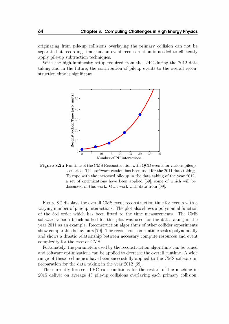
64 Chapter 8. Computing Challenges in High Energy Physics
originating from pile-up collisions overlaying the primary collision can not beseparated at recording time, but an event reconstruction is needed to efficientlyapply pile-up subtraction techniques.
With the high-luminosity setup required from the LHC during the 2012 datataking and in the future, the contribution of pileup events to the overall recon-struction time is significant.
0 5 10 15 20 25 30 35 40Number of PU interactions
0
10
20
30
40
50
Rec
onst
ruct
ion
Tim
e[a
rb.u
nits
]
Figure 8.2.: Runtime of the CMS Reconstruction with QCD events for various pileupscenarios. This software version has been used for the 2011 data taking.To cope with the increased pile-up in the data taking of the year 2012,a set of optimizations have been applied [69], some of which will bediscussed in this work. Own work with data from [69].
Figure 8.2 displays the overall CMS event reconstruction time for events with avarying number of pile-up interactions. The plot also shows a polynomial functionof the 3rd order which has been fitted to the time measurements. The CMSsoftware version benchmarked for this plot was used for the data taking in theyear 2011 as an example. Reconstruction algorithms of other collider experimentsshow comparable behaviours [70]. The reconstruction runtime scales polynomiallyand shows a drastic relationship between necessary compute resources and eventcomplexity for the case of CMS.
Fortunately, the parameters used by the reconstruction algorithms can be tunedand software optimizations can be applied to decrease the overall runtime. A widerange of these techniques have been successfully applied to the CMS software inpreparation for the data taking in the year 2012 [69].
The currently foreseen LHC run conditions for the restart of the machine in2015 deliver on average 43 pile-up collisions overlaying each primary collision.

8.2. Challenges for Current and Next-generation HEP Experiments 65
This means that the average pile-up of 20 during the 2012 data taking is morethan doubled. The design proposals for a possible high-luminosity LHC estimatethe average pile-up collisions to be at 100 [71].
8.2. Challenges for Current and Next-generationHEP Experiments
As described in this chapter, the computing challenges will increase for today’s andfuture collider experiments as the research goals become more sophisticated. Tostill be able to provide online triggering, event reconstruction and Monte Carlosimulation with the best possible physics performance, available computing re-sources must be utilized to the fullest and possible new platforms must be evalu-ated.
In this document, techniques to better utilize the available hardware will beintroduced and performance improvements in the CMS reconstruction softwareand Geant4 simulation suite will be discussed in chapter 10.
Furthermore, a fast, GPU-based method to reconstruct particle tracks measuredin the complex CMS detector will be described in chapter 11.


Chapter 9Modern CPU and GPU architectures
Modern central processing units (CPU) are highly sophisticated integrated circuitswhich evolved significantly during the last 50 years of semi-conductor development.During this time, one of the major dimensions of improvement was the internalclock frequency of CPUs.
The Intel 4004, one of the first fully integrated CPUs, was released in 1971 andwas operated with a clock frequency of 740 kHz. Comparing this to the 4.0GHzprovided by a modern Intel Xeon EC3 CPU, introduced in the year 2013, anincrease of almost factor 6000 in clock frequency was realized.
Figure 9.1.: CPU clock speed, transistor count and cache size over the last 40years [72].
67

68 Chapter 9. Modern CPU and GPU architectures
While this gain in clock rate improved the computational throughput, the num-ber of transistors also increased significantly over the years. This developmentfollows the observation coined as Moore’s law, stating that the number of func-tional components (transistors) on one physical chip approximately doubles everytwo years [73].
While at first glance, both scaling regimes, frequency and transistor count, allowto increase the processing power, one comes with a significant drawback.
The power consumption of the entire CPU is highly dependent of the clockfrequency. This relation can be approximated by the formula [74]
P = CV 2F (9.1)
where P is the consumed power, C the capacity of the CPU circuits, V thevoltage and F the clock frequency.
Increasing the frequency also increases the power consumption on the chip.Despite smart power management systems in modern CPUs, the excess heat gen-erated by the chip must be dissipated. Once a certain clock frequency has beenreached, it is not feasible, neither efficient, to generate more and more heat on thechip. For this reason, the CPU vendors ceased to increase the clock count aroundthe year 2002. This allows to limit the thermal design power (TDP), which is themaximum heat generated by the chip.
Figure 9.1 plots the CPU clock speed, TDP, transistor count and cache sizeof Intel processors ordered by their release date. The plateau in clock frequency,which has been reached around 2002, is clearly visible.
In contrast to clock frequency, the transistor count can still be increased aspredicted by Moore’s law. Therefore, the primary focus of chip designers now restson optimizing the usage of the available transistors to increase the computationalpower of the chip.
The increased number of transistors can be employed, among other uses, toincrease the register size. While the Intel 4004 was a 4-bit CPU, most moderndesktop and server CPUs have a 64-bit wide architecture. This enables the CPUto process more data during one clock cycle. Additional facilities like fast, on-chipmemory caches and smarter instruction processing can also be implemented asmore transistors become available.
This led to the introduction of super-scalar processors. CPUs supporting thisfeature take a serial stream of machine instructions as input, decode and analyzethem for data-interdependencies. Instructions which are independent of each otherare scheduled for parallel execution. To facilitate this, such CPUs have multipleexecution units which can either perform arithmetic or memory operations. Thebenefit is, that multiple machine instructions can be processed during the cycleand the overall throughput of the CPU increases.
Furthermore, multiple compute cores can be implemented with the available

9.1. Vector Units in Modern CPUs 69
transistors on one physical package. This allows to distribute computations amongthe many cores, decrease the clock frequency and thus lowering the total energyconsumption, and therefore the generated heat, of the whole system. Since in-creasing the CPU frequency is not feasible any more, employing multiple CPUcores became one of the primary ways to achieve the performance increase avail-able in modern-day micro-processors.
9.1. Vector Units in Modern CPUs
Another possibility to increase the computational power of one processing coreis to handle more data during one clock cycle. In this respect, vector units canapply one instruction on a whole range (vector) of input values. On a conceptuallevel, the term Single Instruction Multiple Data (SIMD) [75] is used to describethis type of processing.
Although modern SIMD instruction sets also provide operations on integer andbitwise inputs, the focus will be on operations on floating point numbers in thefollowing as these are prominently used in HEP applications. The IEEE 754standard defines the representation of floating-point numbers in binary form [76].It also defines various levels of precision of these representations. In the follow-ing, the single-precision (using 32 bits) and the double-precision (using 64 bits)representations will be used.
While the SIMD concept has been applied to scientific computing since manyyears, it was introduced in the commodity CPU market by Intel with the MMXinstruction set in the late 1990s. Since then, the compute capabilities of theSIMD instruction sets have greatly improved. Following MMX, the SSE2, SSE3and SSE4 instruction sets were developed and introduced 128-bit wide registers,allowing 4 single-precision float values to be processed in one instruction.
The most recent SIMD instruction set is the AVX2 specification and features aregister size of 256-bit, allowing to process 8 single-precision float values in parallel.This results in a theoretical speedup of a factor 8 for floating point operations.In reality, the actual speedup is lower as there is always some overhead involvedwhen loading the values into the vector registers and some parts of the processingwhich can not be expressed with vector instructions.
Virtually all consumer x86 CPUs shipped since the year 2002 support at leastthe SSE2 instruction set. Therefore, SSE2 can be considered the lowest commondenominator when deploying applications compiled with SIMD support.
Figure 9.2 illustrates the register size of the SSE2 and AVX instruction sets andhow they can be populated with either single or double precision values.
The SSE and AVX specifications sets offer a wide variety of instructions, buta special focus has been put on processing floating point numbers of single anddouble precision. As a lot of the simulation and reconstruction code in HEP ap-

70 Chapter 9. Modern CPU and GPU architectures
SSE / SSE2
AVX
128 bit 256 bit
double double
double double double double
sin gle
Register Size
sin gle
sin gle sin gle sin gle sin gle
Figure 9.2.: Vector register size of the SSE/SSE2 and AVX instruction sets. TheSSE/SSE2 registers can either contain four single precision or two dou-ble precision floating point values. The AVX registers can hold twiceas many for each data type.
plications is using floating point data heavily, these instruction sets are especiallybeneficial to increase the runtime performance of these applications.
However, to take advantage of this additional computing power, the softwareneeds to be adapted to use the SIMD instruction during its computing operations.
Chapter 10 will discuss how existing HEP applications can be adapted to benefitfrom the vector instructions and the runtime improvements which can be achieved.
9.2. Multi-Core Design
Another possibility to increase the throughput of one physical CPU is to integratemultiple independent processing cores into one physical micro-processor. Whilethese cores share the same infrastructure, like connection to main memory, coolingand power supply, they can have their own computation units, registers and firstlevel caches.
This allows the CPU to execute multiple instruction streams at the same timeand can increase the computation capabilities of the the CPU significantly. Intheory, the throughput can be increased be a factor N for a CPU with N cores.The speedup in real applications highly depends on implementation details andmemory access patterns of the parallel application.
Early consumer CPUs started to use the Simultaneous Multi-Threading (SMT)technique to implement a fast, hardware-supported context-switching between twoinstruction streams on one physical core. Intel’s implementation of the SMT con-cept, named hyper-threading, is widely available in Intel’s product palette todayand complements also multi-core CPUs. The performance improvements reporteddepend highly on the actual workload and range from almost no improvement toup to 20% in alogrithm runtime [77][78].

9.2. Multi-Core Design 71
Modern Intel Ivy Bridge server CPUs offer up to 15 physical cores, which mul-tiplies to 30 virtual cores when hyper-threading is enabled.
Nowadays, operating systems provide a sophisticated process scheduler to dis-tribute the running process in the best possible way to the CPU cores. For thisreason, a lot of existing applications can benefit from the multi-core capabilitieswithout specifically supporting this feature the in their software design.
Multiple process instances of the same application can be started, wherein eachinstance uses only one CPU at a time and the operating system distributes therunning processes across the available cores.
In the case of event simulation and reconstruction in HEP in general, and inCMS specifically, distributing the input task across multiple processes is feasibleas the individual event are not interdependent. This technique is used in CMScomputing centers to fully load also multi-core CPUs.
The price to pay for this approach is the increased memory consumption becauseeach process has to have its own, dedicated memory region to store constantdata, like the detector geometry or magnetic field maps. While the multi-processapproach in HEP applications is feasible if the ratio between available systemmemory and CPU cores is around 2 GB RAM per CPU core, it becomes harderto maintain if more and more CPU cores become available, but the amount ofmemory does not increase with the same rate.
Chapter 11 documents how track reconstruction algorithms can be implementedthat are able to take the parallel nature of modern CPUs into consideration andis able to use many CPU cores from within one process. This allows the sharingof constant resources, like detector geometry magnetic field map, and reduces thememory consumption when using many CPU cores at the same time.

72 Chapter 9. Modern CPU and GPU architectures
9.3. Massively-Parallel Graphics Processing Units
From the field of computer game graphics originates a very different, in someways much more radical, approach to reach the highest possible throughput withthe available transistors. Instead of employing a high clock frequency to achieve ahigh throughput, Graphics Processing Units (GPU) rely on many small processorswhich work on the compute task in a parallel fashion. This allows for a high data-throughput with a low energy-consumption because a limited clock frequency issufficient.
By now, the benefits of this processing architecture have been recognized alsooutside of the gaming community and GPUs are used in a wide area of applica-tions, including signal processing, engineering simulation, weather prediction aswell as theoretical and experimental physics.
One of the leading vendors of GPU devices, both targeting computer gamingand scientific applications, is Nvidia. This company offers the PCI extensioncard Tesla K40, designed for HPC computing. Compared to the ∼ 2GHz clockrate used in modern CPUs, this card employs a relatively low base clock rate of745MHz, but offers 2880 parallel processor cores [79].
(a) Picture of the Nvidia TeslaK40 PCI express extensioncard [80]. (b) GK110 full chip block diagram [79].
Figure 9.3.: Picture of the Nvidia Tesla K40 card and a diagram of the GK110 chipdiagram.
A picture of the Tesla K40 extension card can be seen in figure 9.3a. The chipschematic of the Kepler architecture GK110, which is underlying the K40 product,can be seen in figure 9.3b. The main building blocks of this design are up to 15streaming multi-processors (SMX). These are independent processor with 64 Kbof shared memory each and 192 individual CUDA processing cores. [79].
Each of the streaming multi-processors can execute up to 2048 parallel threadsof execution, resulting in the capability of a GPU to process the workload in a

9.3. Massively-Parallel Graphics Processing Units 73
massively parallel fashion. The Tesla K40’s on-chip memory is supplemented by12 GB of on-board RAM which are connected via a memory bus with a bandwidthof 288GB/s [80].
With this hardware layout, the Tesla K40 card is able to deliver a peak singleprecision performance of 4.29 teraflops and a peak single performance for doubleprecision of 1.43 teraflops.
Compared to the 100 gigaflops provided by an Intel Core i7 Sandy-Bridge CPU,clocked at 3,4 GHz and having 4 cores, the GPU offers a significant gain in theo-retical peak performance.
2000 2002 2004 2006 2008 2010 2012 2014Release Date
10
100
1000
10000
Peak
Perfo
rman
ce[G
FLOP
S]
Ti500
FX 5900
7950 GT8800 GTX
GTX 285GTX 580
GTX 680GTX 780
Pentium 4 3.4GhzPentium D 840
QX6700 i7-965
i7-3960X
i7-4770K
Peak Performance over Release Date
NVIDIA GPUsIntel CPUs
Figure 9.4.: GPU and CPU single precision peak performance comparison [81].
Figure 9.4 shows the plot of the peak performance of GPU and CPU products,ordered by their release date. Both, CPUs and GPUs profited from the increaseof compute capabilities along the years. Only judging by peak performance, theGPUs are able to provide about an order of magnitude more compute power andthis trend is stable across the last 10 years.
Chapter 11 describes a method to perform particle track reconstruction onGPUs, the necessary adaptions and the gains which are possible for HEP work-loads by using GPUs.

Chapter 10Vectorization Potential for HEPApplications
Floating point computations are an important ingredient to almost every HEPapplication. Significant time is spent with floating point operations and the eval-uation of mathematical functions like the exponential and logarithmic functions.Therefore, taking advantage of the vector units in modern CPUs is a possible wayto improve the runtime performance.
However, C++ code needs to be adapted to conform with the flat data struc-tures required by vector operations. For big HEP application packages like CMSSW,which consists of around 5 million lines of code and many thousand locationswhere floating point computations are performed, such adaptations would requirea major rework of the code base.
However, other ways exist to support vector units in applications. One optionis to provide a fast and vectorized implementation of often used mathematicalfunctions and use them instead of the default ones provided by the system libraries.This process and its benefits will be described in section 10.2.
Furthermore, especially compute-intensive hot-spots can be detected and sped-up using vector instructions. This process will be described in section 10.5.
10.1. Introduction to Vector Unit Programming
Although the SIMD instruction sets are a well-established feature of CPUs forsome time, these extended functionalities could only be accessed by programmerswilling to interleave their high-level C or C++ source code with quasi-assembler in-structions called compiler intrinsics. The SSE2 and AVX technologies use differentinstructions. If all must be supported, the same algorithm has to be implementedseveral times.
75

76 Chapter 10. Vectorization Potential for HEP Applications
Modern compilers, like the GNU Compiler Collection (GCC) [82], provide thepossibility to transform regular C or C++ source code into vector operations.This process is called auto-vectorization and is transparent to the programmer.
The CMS Collaboration opted for the usage of open-source software technologiesand therefore relies on the GCC compiler to build the complete CMSSW softwarestack. The presented results were achieved by using the GCC version 4.6.1, if nototherwise stated [78].
The benefits of using the auto-vectorization features of modern compilers in-stead of low-level intrinsics are manifold. The algorithms can still be expressedas high-level C/C++ code, which brings advantages for the development andmaintainability. In addition, a programmer without SIMD-expertise is able tounderstand and extend the algorithms.
Furthermore, existing algorithms can be adapted to be auto-vectorized by thecompiler. If intrinsic instructions are used, the algorithm must be reimplementedfrom scratch using the dedicated SIMD commands.
Arguably, the biggest advantage is portability. Once the algorithm can beauto-vectorized, the compiler is able to generate machine code for every availableSIMD instruction set and thus support all hardware architectures. Also futureSIMD specifications can be supported by simply upgrading to a new version ofthe compiler. Therefore, an existing auto-vectorizable C/C++ code fragment isguaranteed to benefit from advancements of the SIMD technology in upcomingmicroprocessors [78].
A polynomial of the order 3 can serve as a basic case to illustrate the auto-vectorization process and possible runtime gains. The code listing below showsthe C++ code fragment which computes this polynomial for a list of input values.This code was compiled with GCCwithout vectorization (scalar), SSE and the AVXinstruction set.
1 . . .2 std : : vector<double> x ( ArraySize ) ;3 std : : vector<double> y ( ArraySize ) ;4 . . .5 for ( size_t i = 0 ; i < ArraySize ; ++i )6 {7 y [ i ] = a_3 ∗ ( x [ i ] ∗ x [ i ] ∗ x [ i ] )8 + a_2 ∗ ( x [ i ] ∗ x [ i ] )9 + a_1 ∗ x [ i ] + a_0 ;
10 }11 . . .
The runtimes for a varying size of the input element list was measured for thethree compiled versions. The results obtained when executing the program on a

10.2. The VDT Mathematical Library 77
Intel Core i7-3930K CPU can be seen in figure 10.1. For this simple example,the auto-vectorization performs very well and the compiler is able to generatevectorized code targeting the selected instruction set. The SSE version is about1.5 times faster than the non-vectorized, scalar version. Using the AVX instructionset, a speed improvement of a factor 3.3 can be achieved with respect to the scalarversion.
0 1000 2000 3000 4000 5000 6000 7000 8000 9000Element Number
0
10
20
30
40
50
Runti
me [
ms]
SSE 4.2
AVX
Scalar
Figure 10.1.: Computing a basic polynomial of the 3rd order using either no vector-ization (scalar) or various types of vector instructions(SSE 4.2, AVX )shows significant decreases in the overall runtime when using the vec-tor intsructions.
Furthermore, existing algorithms can be adapted to be auto-vectorized by thecompiler. If intrinsic instructions are used, the algorithm must be reimplementedfrom scratch using the dedicated SIMD commands.
10.2. The VDT Mathematical Library
Analysis shows that existing HEP applications packages spend a significant amountof time in evaluating mathematical functions like logarithm, exponential, sine, co-sine and others. For the Geant4 material simulation of the CMS detector, between12 and 30 percent of the overall runtime can be attributed to mathematical func-tions [78]. For the CMS event reconstruction, around 9 percent of the runtime isspent evaluating mathematical functions [78].

78 Chapter 10. Vectorization Potential for HEP Applications
10.2.1. Existing Mathematical Libraries
The system math library shipped with most Linux distributions is called libm [83]and offers a guaranteed accuracy but is not optimized for the use with vectorunits. Optimized libm replacements are offered, among others, by Intel [84] andAMD [85]. They provide single and double precision floating-point mathematicaloperations which guarantee a certain accuracy in relation to the libm implemen-tation. Both implementations are closed source and in the case of Intel requirethe purchase of a license.
10.2.2. Introducing the VDT Library
To allow the developers of CMS and the wider scientific community to benefit froma fast and vectorized mathematical library, the decision was taken to develop aroyalty-free and open-source implementation within the CMS and CERN softwaregroups.
At the basis of the VectoriseD maTh (VDT) library [78] is the implementationintroduced by the Cephes library[86]. The implementation uses the Pade approx-imants which have been adapted and re-engineered for vdt to be auto-vectorizedby modern compilers. In Pade approximations, the function to compute is ex-pressed by a rational function with an arbitrary order. The independent terms inthe Pade approximation allow for a fast computation, even in scalar mode, as theterms can be distributed over the execution units of super-scalar CPUs.
The vdt library provides fast and auto-vectorizable implementations in singleand double precision floating point for the mathematical functions sin, asin, cos,acos, sincos, tan, atan, atan2, log, exp and 1/sqrt. These functions are pro-vided in C++ header files, which allows the compiler to inline the function body.This allows the compiler to apply its optimization passes not only on the mathe-matical function, but also incorporate the surrounding code. This can potentiallyresult in better optimized and larger blocks which can be auto-vectorized.
The vdt library is provided as open-source under the GNU Lesser General PublicLicense (LGPL3) licence [87]. This allows users to include vdt in open-source aswell as commercial products free of charge. The vdt source code and furtherdocumentation can be downloaded on the project website [88].
As the vdt library is provided as a source code release and does only rely onthe C++ standard, it can be compiled with a variety of compilers and hardwareplatforms. This library design allows to achieve the maximum portability, bothin terms on vector instruction set and machine architecture. The library hasbeen successfully compiled with the GCC and clang compilers for the SSE andAVX instruction set on x86 CPUs and for the ARM platform. As the SIMDinstructions will be generated by the compiler, highly-optimized machine codecan be generated for each platform.

10.3. Speed and Accuracy Comparisons for VDT 79
10.3. Speed and Accuracy Comparisons for VDT
The two primary criteria when designing vdtwere the speed improvements withrespect to the glibC libm and very good accuracy of the approximation.
The quality of the approximation can be best validated by comparing bits inthe floating point representation itself. Floating point numbers in the IEEE rep-resentation [76] are expressed by a sign bit (s), a mantissa (m) and an exponent(e). An arbitrary floating point number (F) within the range of the exponent cannow be written as:
F = s ∗m ∗ 2e (10.1)
To compare the quality of the vdt approximation, the number of differing bitsbetween vdt and libm in the mantissa, starting at the least significant one, iscompared.
Table 10.1 compares the accuracy of vdt to libm as reference. The second col-umn lists the maximum number of differing bits starting from the least significantbit in the whole validation run. This number is a measure for the most pessimisticscenario possible when using vdt as a replacement for libm. The column number3 lists the number of differing bits, averaged over the whole test sample. Thisshows, that the maximum difference estimates are corner cases and that, on av-erage, the amount of different bits is well below 1.0 for all functions implementedby vdt.
Figure 10.2a and 10.2b shows the evaluation of the accuracy of vdt with re-spect to the libm reference implementation for a selected input number range of[0, 5000] for the double precision log function. As visible in figure 10.2a, the vdt
approximation results in either the same output values or differs by only one bitfor the predominant part of the input numbers evaluated.
Figure 10.2b visualizes the quality of the vdt approximation depending onthe sector of the input numbers. While the guaranteed maximum divergence oftwo bits is uphold throughout the whole interval, the quality of the approximationmight change. Around the input number 1000, the approximation does not divergemore than one bit. In contrast, around the number 3500, more 1-bit and 2-bitdiscrepancy can be observed.
More validation plots of the vdt accuracy can be found in appendix A.
Table 10.2 lists the execution speed of the implemented math function forlibm and two different compile options for vdt. The scalar option is to com-pile vdtwithout any vector instructions. This is the lowest common denominatorand will run on every x86 system. The second option listed in table 10.2 is stillscalar, but uses the fuse multiply add (FMA) instruction introduced in the mostrecent Intel Haswell architecture. This machine code can perform a multiply andan add operation on a floating point number with one instruction.

80 Chapter 10. Vectorization Potential for HEP Applications
Differing Bits0 5 10 15 20 25
#
410
510
(a) Histogram of the maximum number ofdiffering bits of the vdt approximationwrt. to the libm reference implementa-tion
0
500
1000
1500
2000
2500
3000
Input0 1000 2000 3000 4000 5000
Dif
feri
ng
Bit
s
0
5
10
15
20
25
(b) Frequency of the maximum number ofdiffering bits of the vdt approximationwrt. to the libm reference implementa-tion for the evaluated input range
Figure 10.2.: Both plots show the evaluation of the approximation accuracy ofvdt with respect to the libm reference implementation for the doubleprecision log function. 500.000 random input values, uniformly dis-tributed in the the considered range [0, 5000] were used for this study.
Table 10.1.: Accuracy and interval of definition of vdt compared to the libm refer-ence implementation for double precision [89].
Function Interval of Definition Max. differing bits Avg. differing bitsExp [−708, 708] 2 0.14Log [0, 1e307] 2 0.42Sin [−2π, 2π] 2 0.25Cos [−2π, 2π] 2 0.25Tan [0, 2π] 2 0.35Asin [−1, 1] 2 0.32Acos [−1, 1] 8 0.39Atan [−1e307, 1e307] 1 0.33Atan2 [−1e307, 1e307] 2 0.27Isqrt [0, 1e307] 2 0.45
All runtime numbers have been measured on a Intel Core i7-4770K CPU runningat 3.50GHz. The operating system was Scientific Linux 6 with the GNU libc

10.3. Speed and Accuracy Comparisons for VDT 81
version 2.12-1.107.el64.4 and the vdt functions were compiled with GCC version4.8.
The significant speed improvements provided by vdt is visible in table 10.2.Due to implementation details, the vdt speedup is different for each mathematicalfunction. The runtime for the exp function, which is one of the most widely usedin HEP software, is improved by a factor of almost 13. The log function is sped upby a factor of almost 3. The FMA instruction brings slight runtime improvementsto most of the vdtfunctions.
Table 10.2.: Runtime comparison of double precision math functions between vdt inscalar mode and glibC libm. The time is in nanoseconds per calculatedvalue [89].
Function libm [ns] vdt scalar [ns] vdt scalar FMA [ns]Exp 102 8 5.8Log 33.3 11.5 9.8Sin 77.8 16.5 16.5Cos 77.6 14.4 13.2Tan 89.7 10.6 8.9Asin 21.3 8.9 6.9Acos 21.6 9.1 7.3Atan 15.6 8.4 6.7Atan2 36.4 19.9 18.9Isqrt 5.7 4.3 2.8
Even though the scalar version already shows significant speed improvements,the may primary design goal of vdt is to take full advantage of the available vectorinstruction sets. Table 10.3 compares the runtime of the scalar version with twoflavors of vector instruction. The same C++ source code is evaluated here, butmerely the compiler was instructed to generate machine code for the indicatedvector architecture.
The SSE vector instruction set can be considered the lowest common denomi-nator, as it is supported by virtually all x86 machines used in the HEP communitytoday. Here, the expected time 2 decrease in runtime, which can be expected withdouble precision numbers, is achieved by most of the vdt functions, and exceededby some.
Using the more powerful AVX2 instruction set, all of thevdt functions are ableto achieve a better runtime, but only some ( exp, sin, cos ) are actually twiceas fast as with SSE. For some ( asin, acos ) a modest increase can be achievedwith larger vector registers because the vector opportunities in the mathematicalexpressions can already be almost fully expressed with SSE.

82 Chapter 10. Vectorization Potential for HEP Applications
Table 10.3.: Runtime comparison between vdt in scalar mode and the librarycompiled to take advantage of the SSE and AVX2 vector instructionsets [89].
Function vdt scalar [ns] vdt SSE [ns] vdt AVX2 [ns]Exp 8 3.5 1.7Log 11.5 4.3 2.2Sin 16.5 6.2 2.6Cos 14.4 5.1 2.3Tan 10.6 4.4 3.2Asin 8.9 5.8 5Acos 9.1 5.9 5.1Atan 8.4 5.6 5.1Atan2 19.9 12.7 8.4Isqrt 4.3 1.8 0.4
10.4. Application of vdt to Geant4To study the real-world gains possible with vdt on big software packages, twoapproaches are possible:
• Replace hot-spot mathematical functions with the vdt version
Modifications to specific areas of the code are necessary to call the vdtfunctions.
• Replace all calls to mathematical functions by their respective vdtversion
The library pre-load technique can be used to fully replace all calls to selectedfunction without recompiling the targeted application. The dynamic linkingin Linux system already offers this functionality.
For the following study, the pre-load technique was employed to replace all callsof Geant4 to libm with their respective vdt counterparts. This allows for annon-intrusive validation and it is conservative, both in terms of runtime improve-ments and physics performance. Due to the nature of dynamic linking, whichhappens during runtime and not compile time, the compiler is not able to inlinethe vdt mathematical functions and apply further optimizations. Secondly, byreplacing all mathematical functions, the vdt approximations will be used in allareas of Geant4 and potential changes to the physics performance can be easilyspotted during the validation process.
For the following tests, top anti-top events with a center-of-mass energy of8 GeV were simulated with Geant4 within the full CMS geometry.
10.5. Improving the Runtime of CMS Vertex Clustering 83
The physics objects of the libm and vdt versions of Geant4 have been comparedusing the full suite of the CMS validation workflow, which contains more then100.000 histograms. The output of the vdt version shows is compatibile to thelibm reference implementation.
Two different type of workflows have been studied. The first workflow is toevaluate speedup achieved, when Geant4 runs for an extended amount of time, atypical scenario when performing Monte Carlo production on the LHC computinggrid. For this, 50 events were simulated with Geant4 and an overall speedup of6.6% can be achieved with vdt.
Measuring the runtime of just one event simulated by Geant4 shows how thevdtlibrary can improve the startup time. When using vdt, the for event is pro-cessed 25.0% faster then when using libm [89]. The speed improvements availablewith vdt are more pronounced during the first event, as values need to be initial-ized, which make heavy use of mathematical functions.
With the most recent Geant4 10.0 release, the vdt library was introduced toimprove the runtime of the overall application [90]. This will enable the speedbenefits of vdt to all users of Geant4, independent of the operating system orplatform.
10.5. Improving the Runtime of CMS VertexClustering
As described in section 7.7, the CMS event reconstruction relies on a determin-istic annealing algorithm [58] to compute the location of the primary verticesin one event. Especially with an increasing number of pileup-interactions, thisreconstruction step in CMSSW amounts for a considerable part of the overall ap-plication runtime [89]. To prepare for the 2012 data taking conditions, the runtimeperformance of this algorithm needed to be improved. Due to the intensive useof floating point computations in this algorithm, it is an ideal case to apply theauto-vectorization technique.
After adapting two compute intensive loops of the deterministic annealing al-gorithm, the GCC compiler was able to auto-vectorize the performed mathematicaloperations. Furthermore, a large fraction of the algorithm runtime is spent inthe evaluation of the exponential function. The previously introduced fast andauto-vectorizable exponential function of the vdt library was used to speedup thiscalculation. The decision was taken to use the SSE instruction set in the compila-tion process, as it is available on all processors installed in the data centers whichprovide computing resources to the CMS collaboration.
The physics output of the improved algorithm has been fully validated usingthe extensive set of quality monitoring tools of CMS and a perfect agreementwith the previous, scalar implementation is observed. Neither the vectorization

84 Chapter 10. Vectorization Potential for HEP Applications
5 10 15 20 25Number of PU interactions
0.0
0.1
0.2
0.3
0.4
0.5
0.6
0.7
0.8
0.9
Clu
ster
ing
Tim
e[s
]
ScalarVectorizedVectorized + VDT
(a) Runtime of the vertex clustering for var-ious pile-up scenarios and implementa-tions.
5 10 15 20 25Number of PU interactions
1.5
1.6
1.7
1.8
1.9
2.0
2.1
2.2
Spee
dup
wit
hV
ecto
riza
tion
and
VD
T
(b) Speedup of the vectorized vertex clus-tering using vdt with respect to thescalar version.
Figure 10.3.: Runtime and speedup of the scalar and the vectorized implementationsand the vectorized version using the vdt library for different pile-upcontent in the event. The mean pile-up interactions for CMS was 20in the year 2012.
process, nor the application of the approximate exponential function provided bythe vdt library did influence the physics performance.
Figure 10.3a shows the mean runtime of the scalar and the vectorized imple-mentations and the vectorized version using the vdt library for different pile-upcontent in the event. For this runtime study, 10000 Events recorded by the CMSdetector during the year 2012 with a center-of-mass energy of
√s = 8 TeV have
be used to quantify the runtime of the implementations.
Figure 10.3b displays the speedup which can be achieved by the vectorizedimplementation with respect to the default one. The benefits of vectorization areespecially pronounced for more pile-up contribution, meaning more particle tracksin the event. In these cases, the vertex clustering algorithm has to iterate over abigger set of input tracks and perform the computations which have been sped-upby the use of vectorization and vdt. Starting with 16 pile-up interactions thespeedup is more than a factor of 2. The average number of pile-up interactionsper event in the year 2012 for CMS was 20 [22].
The SIMD-enabled version of the vertex clustering algorithm was used for theoffline recontsruction of the LHC data in the year 2012. This allowed to achievean excellent vertexing performance in high-luminosity conditions while stayingwithin the runtime envelope assigned to the vertex clustering.
The LHC run conditions for the restart in the year 2015 will increase the averagepile-up collisions per event to 43. With the goal to achieve an excellent vertexingperformance in these conditions, the offline reconstruction will continue to use the

10.5. Improving the Runtime of CMS Vertex Clustering 85
SIMD-enabled vertex clustering presented here.Also the online reconstruction used in the high-level trigger faces a more dif-
ficult measurement environment with the increased pile-up contribution. Due tothe vectorization optimizations presented here, the deterministic annealing vertexclustering became a possible candidate to be used in the more time-constrainedHLT farm. Studies are underway to estimate to which extend the DA vertex clus-tering can improve the physics performance in the HLT compared to the faster,but less elaborate algorithm used before.


Chapter 11Fast track reconstruction for massivelyparallel hardware
As outlined in chapter 9, GPUs can provide a significant advantage in terms offloating point peak-performance and energy consumption compared to classicalCPUs. This is made possible by the radically different design decisions taken bythe GPU manufacturers, above all to use many basic compute cores instead ofonly a few, but very powerful ones.
These differences in design are reflected in the programming techniques neces-sary to fully exploit the capabilities of GPUs. Complex algorithms and programs,which have been designed and optimized for classical CPUs, are likely to notperform well on GPUs. Some of the fundamental features GPU-adapted imple-mentations must address are:
Massively parallelThe NVIDIA Tesla K40 card provides 2880 parallel processor cores [79], morethan a factor 100 of what is provided by a even high-end CPUs. Algorithmsmust be designed and implemented to provide sufficient workload for all of theseprocessors to be busy at the same time. Failing to do so will result in parts of theGPU being idle and wasting bought resources, and therefore money.
While classic CPUs can be fully loaded with around 10 parallel threads, GPUsrequire 1.000s, even better 10.000s, parallel threads of execution.
Memory layout and size limitationsThe high-end NVIDIA Tesla K40 card has up to 12 Gb of on-board RAM, whichis available to application usage. This memory is shared between all processingcores, the access has a high latency and access operations from multiple cores atthe same time must be serialized to protect for memory corruption. To allow forfaster memory operations, each multi-processor has its own shared memory, which
87

88 Chapter 11. Fast track reconstruction for massively parallel hardware
can be exclusively accessed by threads running on it. In case of the NVIDIA TeslaK40 card, the shared memory is 64 kb large.
To achieve peak performance, this memory region must be managed properly tohave the data necessary for a computation available close and fast to the processingcore using it.
Furthermore, memory buffers on the GPU must be pre-allocated and have a pre-determined size. Some high-end cards support dynamic memory allocation duringexecution on the GPU. This functionality is only available on a small subset ofhardware and is not portable to other vendors than NVIDIA.
Data transfer overheadThe on-board memory of the GPU is logically and physically separate from thehost-PCs memory region. Therefore, necessary data needs to be copied from thehost to the GPU prior to the computation and vice versa.
GPU implementations must make sure that the data-transfer time is well amor-tized by the actual work done on the GPU. This latency can also be hidden, bystreaming data continously to the GPU, while the previous computation is still inprogress.
Floating point precisionThe GPU market emerged from the computer game segment, there was initiallyno need for high-precision floating point operations. Computer graphics workswell with the limited representation of single precision floating point numbers,but many scientific applications require double precision floating point, as theywant to reduce the error introduced by the floating point representation as far aspossible.
Even modern GPUs, which are targeted at the scientific market, are only ableto deliver around one third of their maximum performance in double precisioncomputations. Therefore, an additional performance gain can be achieved whenthe employed algorithms are numerically stable and the single precision floatingpoint representation is sufficient.
External librariesExternal libraries, for example for linear algebra, which are used in a CPU im-plementation cannot be easily integrated into a new GPU implementation. Somemathematical libraries, like cuBLAS [91], exist and can be used in GPU-ports ofexisting software.

11.1. Track Reconstruction on GPU Devices 89
11.1. Track Reconstruction on GPU DevicesThe described characteristics of GPU hardware make it either impossible or hardand with degraded performance to translate CPU-designed reconstruction algo-rithms and implementations to accelerator hardware.
Existing algorithms must therefore be re-evaluated and potentially changed interms of data and control flow to be adapted for GPU hardware.
The CPU-implementation of the current CMS track reconstruction is involvingmany different types of computations and features a complex control flow. Fur-thermore, a variety of input data is necessary for even the initial seeding stepof the track reconstruction: detector layout, magnetic field and detector mate-rial information. These factors make the current CPU-bound implementation notfeasible to be ported directly to GPU architectures.
This chapter will present a GPU-targeted implementation of the initial trackseeding and discuss how complete tracks can be reconstructed to harness thecompute capabilities of modern GPUs.
11.2. GPU and Accelerator ProgrammingSpecialized programming libraries exist to access GPU and other hardware ac-celerators. The two most popular options are the CUDA platform, provided byNVIDIA, and the OpenCL standard, which is implemented by a variety of vendors.
Both platforms provide a similar set of components:
• Custom compiler
In both OpenCL and CUDA, the program which runs on the GPU can bewritten in dialect of the C language and is translated by a custom compilerto the machine instructions of the actual GPU.
• Host library
This library is loaded inside of the host program running on the CPU and isused to control the memory allocation, data transfer and program executionon the GPU.
• GPU device driver
This component keeps track of all GPUs connected to the host machine andinterfaces the GPUs to the host library.
While both OpenCL and CUDA offer a similar set of features, the most strikingdifference is the reach of these platforms.
The CUDA platform is a product of NVIDIA, and therefore only supportsNVIDIA GPUs. This allows NVIDIA to integrate advanced features, like dynamic
90 Chapter 11. Fast track reconstruction for massively parallel hardware
memory allocation, on the hardware as well as on the software side at the sametime.
The OpenCL platform is an open standard formulated by many industry leadersin the hardware and software domain, among them being Apple, Intel, AMDand NVIDIA. OpenCL’s goal is to support the accelerator hardware of differentvendors without changing the implementation of the program. This aspect ofOpenCL is also named portable performance.
OpenCL-based programs cannot only run on the GPUs of NVIDIA, Intel andAMD, specialized hardware accelerators like the Intel Xeon Phi, but can also beexecuted on x86 CPUs without any changes. This is not possible with the CUDASDK provided by NVIDIA.
In the context of CMS and grid computing, portability to different types ofhardware is an important design constraint. If a capable accelerator device isavailable on a host machine, OpenCL-enabled applications can make use of them.In the fallback case, the CPU can be used to execute the OpenCL programs.
Another important advantage in using OpenCL is the possibility to easily switchor even support different GPU hardware vendors at the same time. The GPUmarket is a very dynamic one, with vendors like Intel, AMD and NVIDIA. By notrelying on one specific vendor, possible price or performance advantages acrossvendors can be better utilized.
These two arguments let to the decision to use OpenCL as the basis for the trackreconstruction implementation. In the following, an introduction to OpenCL andits most important concepts will be given.
11.3. Introduction to OpenCL
Influenced by NVIDIA’s CUDA from the GPU side and by OpenMP, which origi-nates from the classical CPU side, the open OpenCL standard is characterized bya formulation which is abstract enough to support both CPU and GPU computingresources. This is an ambitious goal, since providing an abstract interface togetherwith the possibility to achieve peak performance is a challenging task. OpenCLemploys a strict isolation of the computation work into fundamental units, the ker-nels. These kernels can be developed in the OpenCL C programming language,a subset of the C99 language, with some additional OpenCL specific keywords.In general, these kernels are hardware independent and compiled by the OpenCLruntime when they are loaded. To be able to fully exploit the parallel executionof the kernel code, multiple so-called work items are started to process a set ofinput values. The number of concurrently running work items is determined bythe OpenCL system. How a concrete algorithm can be partitioned into work itemshas to be decided by the programmer.

11.4. clever: Simplified OpenCL Programming 91
11.3.1. Intel OpenCL SDK
As part of the OpenCL consortium, Intel played an important role in creating theOpenCL standard. The Intel OpenCL Software Development Kit (SDK) compilesOpenCL kernels in order to run them on x86-64 CPUs, Intel GPUs and the IntelXeon Phi accelerator PCI board. Code vectorization is exploited to distribute thecalculations of a kernel to the vector units. The most recent release of the SDK,supports the SSE and AVX vector instruction sets.
11.3.2. NVIDIA OpenCL
One of the forerunners of the OpenCL standard is the CUDA system for GPUsby NVIDIA. Since 2009, the NVIDIA graphics driver also supports the OpenCLstandard and can compile and run OpenCL kernels on the graphics card.
11.4. clever: Simplified OpenCL Programming
The CMS reconstruction software has been developed and is maintained by adiverse group of physicists and computer scientists. Therefore it is necessary thatthe source code is accessible to all scientists involved, even if their programmingskills and experience might differ. Furthermore, one algorithm might have beenimplemented by one person but will be modified by changing maintainers over thelifetime of the CMS experiment. For this reason, the amount of expert code, whichcan only be extended by personnel with specific knowledge, should be limited asmuch as possible.
The API provided by the OpenCL framework is based on the C programminglanguage and explicit memory management is required. Furthermore, OpenCLkernels are not syntax checked during the compile time of the host application.They are loaded from text files and compiled during the startup of the host ap-plication. This makes it harder to spot syntax errors as early as possible.
The open-source openclam1 library offers a convenient way to encapsulate OpenCLkernels inside of C++ classes. Using this method, the OpenCL C-based program-ming statements can be conveniently inserted in between regular c++ programlines. This allows for a syntax check of the OpenCL kernels during compile time ofthe host application and no separate text files need to be maintained to hold thekernel’s source code. The development of the openclam library has ceased sincesome years and lacks some desired features like more elegant memory manage-ment. To improve this situation, the clever library has been developed as partof this thesis and builds on the idea of openclam to integrate the OpenCL kernels
1http://code.google.com/p/openclam (19.12.2014)

92 Chapter 11. Fast track reconstruction for massively parallel hardware
within the C++ source code and offers a convenient C++ wrapper for OpenCL’sAPI calls.
The following section will given an overview of the functionalities offered by theclever library. The equivalent C++ source code of the OpenCL API has beenomitted for the sake of compactness but can be found in any OpenCL program-ming introduction.
11.4.1. OpenCL Compute Context CreationThe C++ class clever::context is the main entry point of the clever library. Ifno parameters are supplied to this class, the first OpenCL runtime which is avail-able on the current platform is selected. This object can also be created with a setof configuration parameters to select a specific OpenCL runtime or define whethera GPU or CPU should be used. Once the object of the class clever::context
is destroyed, also all OpenCL resources which have been allocated via this con-text object is automatically released. This provides a programmer-friendly wayto manage the lifetime of OpenCL resources.
Two examples of context creation can be seen in figures 11.1 and 11.2. In thefirst example, a context object is created without further specifying the platformand device type. The second example shows how a compute context can berequested on the NVIDIA platform. If the NVIDIA platform is not available onthe current host, a C++ exception will be thrown.
// create compute context on default platform
clever::context context;
Figure 11.1.: Instantiation of an OpenCL Compute Context on the default Platform.
// create compute context on the NVIDIA platform
clever::context_settings cs ( clever::opencl::PlatformNameNVIDIA( ) );
clever::context context( cs );
Figure 11.2.: Instantiation of an OpenCL Compute Context on the NVIDIA Plat-form.
11.4.2. Memory Management and Data TransferIn most modern programming languages, the lifetime of objects and the memoryallocated to hold their state is either partially or fully handled by the compileror runtime environment. In the C++ language, the memory regions of objects
11.4. clever: Simplified OpenCL Programming 93
which are allocated on the stack of a specific method are automatically releasedonce the stack of the method is left. C++ objects which have been allocated onthe heap must be manually allocated and de-allocated by the programmer, but thelanguage offers convenient constructs to shield the concrete size of memory blocksfrom the programmer. Other languages, like Java, provide a garbage collection,where all allocated memory regions are automatically released once they are notin use any more.
In contrast, all memory buffers holding the input and output of computationsperformed with OpenCL must be explicitly allocated and de-allocated by theprogrammer. This can become especially cumbersome, when OpenCL memorybuffers are used within larger applications, like CMSSW, and must be sharedamong many different modules.
To ease the memory management with OpenCL, the clever library includesC++ classes which take care of allocating OpenCL buffers of the correct sizeinternally. The lifetime of the OpenCL buffer is directly coupled to the lifetime ofthe C++ object, which allows the programmer to apply the same rules he alreadyknows from C++ resource management to control the lifetime of OpenCL memorybuffers. Once the C++ object referencing the OpenCL buffer is destroyed, alsothe underlying memory region of the buffer is released.
Code listing 11.3 shows an example using the clever library’s matrix type toallocate a 5-dimensional matrix with double precision floating point numbers andtransfer a set of values to the OpenCL device.
11.4.3. Programming OpenCL Kernels
The clever library greatly simplifies the development of OpenCL kernel code.In the standard OpenCL framework offered by the vendors, OpenCL computekernels are only syntax checked at the runtime of the host application. Buildingon the ideas of the openclam framework, a set of C++ macros are offered tothe programmer to define the number of parameters passed to the kernel and theprogram code executed with the kernel.
The OpenCL C-language code within the kernel’s function is syntax checkedduring the compile time of the host application. Code snippet 11.4 shows anexample which defines an OpenCL kernel which takes two parameters as input.
The macro KERNEL2 CLASS will create a C++ class which can be instantiatedby the programmer at the time the kernel code must be executed. At this time,the kernel code is compiled with the OpenCL framework and registered with thename add val.More complex kernels, taking more input parameters have been developed usingthis technique, but are not shown here for the sake of compactness.

94 Chapter 11. Fast track reconstruction for massively parallel hardware
clever::context context;
// define 5x5 matrix
typedef clever::matrix<double, 5> TestMatrix;
// don’t set initial value but download it later on
TestMatrix m1( context );
// initialize the matrix entries
m1.fromArray( { 1,0,0,0,0
0,1,0,0,0
0,0,1,0,0
0,0,0,1,0
0,0,0,0,1 } );
// download values to device
m1.from_array(m1_in );
Figure 11.3.: Allocation of a custom matrix data type on an OpenCL compute con-text.
KERNEL2_CLASS( add_val, cl_mem, double ,
__kernel void add_val( __global double * a, const double b )
{
a[ get_global_id( 0 ) ] += b;
});
Figure 11.4.: Definition of a simple kernel with two parameters. The kernel onlyadds a constant value b to the values contained in the input array a.
11.4.4. Executing OpenCL Kernels
Once a C++ object holding the OpenCL kernel has been created, the kernel code isready to be executed on the compute device. To pass all required input parametersto the kernel, the run() method is called. Parameters can either be scalar valuesor pointer to previously created OpenCL memory buffers. The code snippet 11.5displays how one memory buffer (m1) and the scalar number 55 are passed to thekernel. The third parameter is passing the OpenCL work dimension, which definesover how many entries in the m1 memory buffer the kernel will iterate.
For the track seeding implementation on GPU-devices presented in the followingsection, the clever library has been used to simplify memory management andto define and execute OpenCL kernels.

11.5. Track Reconstruction with the Cellular Automaton Method 95
kernel.add_val.run(m1.get_mem(), 55, m1.range() );
Figure 11.5.: Calling an already defined kernel. m1 is the matrix in memory, whichhas been defined before, 55 is the constant which is added to everyelement of the matrix and m1.range() passes the size of the matrixto the kernel execution.
11.5. Track Reconstruction with the CellularAutomaton Method
The cellular automaton (CA) track reconstruction method [92] uses a differentapproach to full track finding than the classical Kalman-method described inchapter 7. In the classical method, initial trajectory seeds (hit pairs or triplets)are generated at the innermost detector layer and subsequently propagated to theouter layers, with compatible hits being added to the tracks.
In the CA-method, triplets are not only generated for the innermost detectorlayer, but for all layers of the detector. Subsequently, compatible triplets onadjacent layers are joined to form a track candidate.
The triplet finding step of the CA-method is a localized operation: only hitdata from three neighbouring detector layers enter the computation. Furthermore,triplets across the whole detector can be generated independently from each other,which allows for a large amount of parallelism in the algorithm.
Additionally, the CA implementation presented here will use cut-based criteriaand parametrize the material effects on the track. This avoids using the Kalman-filter technique in the seeding step, which is known to be numerically unstablewhen using only single precision floating point representation [93]. As the pre-sented implementation can therefore use single precision, the larger performance ofGPUs when processing single precision floating point numbers can be harnessed.
These properties make the CA-method especially interesting to study as a GPUimplementation.
The CA-method can be separated into four stages:
• Hit pair generation
Finding two compatible hits on layer n and layer n-1 which might belong tothe same track.
• Triplet prediction
Using the information from the hit pair, compute the location where thethird hit on layer n+1 is expected.

96 Chapter 11. Fast track reconstruction for massively parallel hardware
• Triplet filtering
Generate triplets using the hit pairs and the compatible hits found on layern+1. Apply quality cuts to decrease the fake rate of the generated triplets.
• Triplet joining
Combine compatible triplets on adjacent layers to form longer track seg-ments.
11.6. Hit Pairs pre-selectionDue to their high number, not all possible combinations of hits on two adjacentlayers can be passed on to the downstream triplet generation. While two hitsallow for only a limited determination of a tacks parameter, their location and theassumption that all tracks originate within a window around the collision pointallow to reduce the possible combinations significantly.
Assuming a hit h2 = (φ2, z2) in the outer layer, the search range for z in theinner layer can be limited to [94][
r1r2
z2 + z0,max
− z0,max, r1r2
z2 − z0,max
+ z0,max
](11.1)
where r1 and r2 are the radii of the detector layers containing h1 and h2, respec-tively. z0,max is the size of the acceptance window in z direction.
Also the change in the φ position between the two hits can be evaluated for theircompatibility with a track originating at the center of the detector. The tracks ofcharged particles are curved in the magnetic field of CMS and they travel along ahelix with radius r, which is related to the transverse momentum pT of the track.A minimum radius rmin can be defined, for the minimum curvature of tracks whichare accepted for the hit pair building.
Furthermore, the maximum transverse impact parameter d0,max is introducedto allow for tracks which do not originate exactly at the origin in the transverseplane.
Using the minimum radius rmin, the accepted ∆φ can then be limited to [94]
|∆φ| ≤∣∣∣∣arccos
(r2
2rmin
)− arccos
(r1
2rmin
)∣∣∣∣+ arctan
(d0,max(r2 − r1)
r1r2
)(11.2)
11.7. Triplet PredictionTo limit the number of third hits combined with the generated hit pair, a predic-tion of the possible positions of the third hit is performed. In a similar fashion

11.8. Triplet Filtering Criteria 97
to the hit pair pre-selection, equations 11.1 and 11.2 are used to compute theaccepted region of the third hit. The origin of the coordinate system is movedto the position of the first hit of the hit pair, and the second hit of the hit pairis used to extrapolate to the possible search window for the third hit. In thiscomputation d0,max needs not be considered as a possible transverse displacementof the track has already been handled by defining the first hit as the origin of thenew coordinate system.
All hits in the third layer, which are in the predicted search window, are selectedas triplet candidates.
11.8. Triplet Filtering CriteriaAdditional filter criteria on the triplet candidates are applied to reject fake com-bination of hits.
Cut on dθ
The differences in θ between the lower half (hit one and two) and second half (hittwo and three) is expected to be zero. The magnetic field in CMS is only affectingthe particle trajectory in the transverse plane. The particle propagation in they-z plane can be assumed to be a straight line. Multiple scattering effects andmeasurement uncertainties still affect the recorded position of the hit. Therefore,a narrow window of acceptance must be available.∣∣∣∣θ′θ − 1
∣∣∣∣ ≤ dθ (11.3)
wherein θ is of the lower half and θ′ of the upper half of the triplet and dθ isthe accepted difference between the two. Figure 11.6 illustrates this cut.
θ
θ'
Figure 11.6.: Definition of θ and θ′ of a triplet in the z-y plane.
Cut on dφSimilar to dθ, an additional cut on dφ can be applied. Contrary to θ, the angle φmight change due to the curvature of the track in the magnetic field. This featuremust be considered when determining the cut value dφ.

98 Chapter 11. Fast track reconstruction for massively parallel hardware
|φ′ − φ| ≤ dφ (11.4)
Figure 11.7 displays a slightly curved trajectory in the x-y plane and the asso-ciated φ and φ′ values.
y
x
φφ'
Figure 11.7.: Definition of φ and φ′ of one triplet in the x-y plane.
Cut on the transverse impact parameterThe previous two filter criteria ensure the triplets to be internally consistent bypreventing kinks in the θ and φ angles. Another criteria to improve the qualityof final triplets is to require tracks to originate in the vicinity of the interactionpoint. To determine this transverse impact parameter - the closest approach ofa track to the detector center - a fit with the three hits included in the triplet isperformed.
In the transverse plane, the trajectory of the charged particles can be approx-imated as a circle which is fully defined by the three triplet hits. The Riemannmethod [95] maps points on circles on to planes and performs a fit in this trans-formed space. Its performance and runtime have been compared to other fittingtechniques for the circle fit use case and found to be up to 40 times faster [95].
Additionally, the program code to implement the Riemann fit is compact andcontains no recursion or complex control flow. These features make this methodespecially suited to be implemented on GPUs.
Once the circle passing through all three hit positions has been computed, thepoint of closest approach d0 to the origin can be easily determined. This allowsto apply a selection with d0,max being the maximum accepted distance from thedetector center.
d0 ≤ d0,max (11.5)
Figure 11.8 displays three hits assigned to a triplet in the transverse plane. Alsovisible is the fitted circle and its transverse impact parameter.

11.9. Determination of Triplet Filter Cuts 99
y
xtIP
Figure 11.8.: The transverse impact parameter of a triplet after all three hits havebeen fitted with the Riemann method.
11.9. Determination of Triplet Filter Cuts
To determine the cut values, a dataset with simulated top pair decays was used.During the of decay the top quarks, many secondary particles are generated andare concentrated in specific regions of the detector. This high track density is a dif-ficult environment for reconstruction algorithms and allows meaningful estimatesof an algorithm’s fake rate.
Cut values have been derived for triplets located on various combinations oftracker layers. These cuts have been balanced to achieve a reconstruction efficiencyof 80%.
0.0 0.1 0.2 0.3 0.4dφ Cut
0.1
0.2
0.3
0.4
0.5
0.6
0.7
0.8
0.9
1.0
Frac
tion
[1]
no cutno cutno cut
RealBackgroundFakerate
Figure 11.9.: The fraction of real, fake and background triplets which pass the dφcut plotted over a range of the cut quantity. For the plot point “nocut”, none of the cuts are applied and all possible triplet combinationsare in the final selection.

100 Chapter 11. Fast track reconstruction for massively parallel hardware
Figure 11.9 shows the triplet finding efficiency for various values of the cutquantity dφ for triplets on the first three detector layers in the barrel region.The background contribution is also plotted which is the percentage of wrongcombinations passing the cut criteria divided by the overall amount of wrongcombinations. The fake rate is the percentage of wrong combinations divided bythe overall number of combinations passing the cuts. These definitions are alsolisted in equations 11.6.
Eff =Npassed
Ngen
Fake =Nfakes passed
Npassed
Bkg =Nfakes found
Nfakes
(11.6)
For the study presented in figure 11.9 only the dφ cut was applied to the inputset of possible triplet combinations. In the actual implementation described below,the three cuts are applied sequentially.
The cut value evaluations of dθ and d0,max for the first three detector layers inthe barrel region can be found in figures B.1 and B.2 in appendix B.
Figure 11.10 shows the efficiency, fake rate and background contribution whenall three triplet filter cuts are applied sequentially on a set of input triplet candi-dates from the first three layers in the barrel tracking detector.
Cut Flow
0.1
0.2
0.3
0.4
0.5
0.6
0.7
0.8
0.9
1.0
Frac
tion
[1]
no cut phi cut theta cut TIP cutno cut phi cut theta cut TIP cutno cut phi cut theta cut TIP cut
RealBackgroundFakerate
Figure 11.10.: The fraction of real, fake and background triplets if all three tripletfilter criteria are applied sequentially.
After all three cuts have been applied, the triplet finding effiency is at 92% witha fake rate of 49%.
In the same manner, optimal cut values have been determined for the otherlayer combinations which are used for triplet seeding. Table 11.1 lists the final

11.10. Investigation on Triplet Joining criteria 101
Triplet Layers dφ dθ d0,max
1-2-3 0.075 0.01 0.52-3-4 0.2 0.2 0.53-4-5 0.4 0.4 1.04-5-8 0.4 0.5 3.5
Table 11.1.: Cut quantities for the dφ, dθ and d0,max triplet filter for all studied layercombinations.
values of the three quality cuts for the studied layer combinations. The more thestudied layer combinations are located in outer regions of the detector, the morethe cuts needed to be relaxed to achieve the targeted triplet efficiency of 80%.
This has three primary reasons:
• The measurement uncertainty of the strip silicon detectors, starting at layerfour, is coarser than the pixel silicon detectors of the first three layers
• The traveled distance between the detector layers is bigger, thus increasingthe effect of track bending
• The distance to extrapolate the trajectory back to the detector center islarger, thus the computed TIP becomes less precise.
11.10. Investigation on Triplet Joining criteria
Once triplets on all layers have been generated, they can be combined to formlonger segments of tracks. In the following, possible combination criteria fortriplets from layers 1-2-3 and layers 2-3-4 will be studied.
To this extent, the three hits associated to a triplet haven been fitted withthe Kalman-method of the CMS reconstruction. Due to the smoothing proceduredescribed in chapter 7.5, the best-estimate of the track state is available at eachof the three hits. This allows to check the triplets for compatible direction andmomentum at each hit they share.
In the following, the three combination criteria, which have been studied, willbe discussed:
Shared hits between tripletsWhen searching for triplets in neighbouring detector layers, triplets which containhits from the same track must share two hits on the two inner layers.

102 Chapter 11. Fast track reconstruction for massively parallel hardware
R
Z
Track
Triplet1
Triplet 2Shared Hits
Figure 11.11.: Illustration of two triples on neighbouring detector layers sharingtwo hits. If both triplets have been generated with the hits from thesame track, as shown here, they must have the two innermost hits incommon.
Figure 11.11 illustrates two triplets, which belong to the same track, sharingtheir inner hits. To determine the hits shared between triplets, no explicit com-putation is necessary. Only the identification numbers of hits included in thetriplets must be compared, which is a very fast operation on CPU and GPU.Only triplet combinations with two inner hits shared are considered for furtherprocessing. This already reduces the amount of input data passed to the morecompute intensive steps which follow.
Charge and momentum compatibilityDue to the Kalman fit of the triplet hits, the charge and momentum of the trackis available at the position of each hit. For both shared hits, the charge dividedby the magnitude of the momentum must be similar. Formula 11.7 is used to cuton this quantity by ensuring the absolute difference between the values of bothtriplets is smaller than dp. The charges q and q′ and the momenta ~p and ~p ′ areof the first and second triplet, respectively.∣∣∣∣ q|~p | − q′
|~p ′|
∣∣∣∣ ≤ dp (11.7)
Direction compatibility
For both shared hits, the direction of the track is expected to be similar, thushaving no kink. Formula 11.7 is used to express this requirement by computingthe magnitude of the difference between the normal vectors ~n and ~n′ of the trackdirection for each triplet. Only triplet combinations for which this quantity issmaller then dx pass this cut and are considered a valid combination of two triplets.
|~n− ~n′| ≤ dx (11.8)
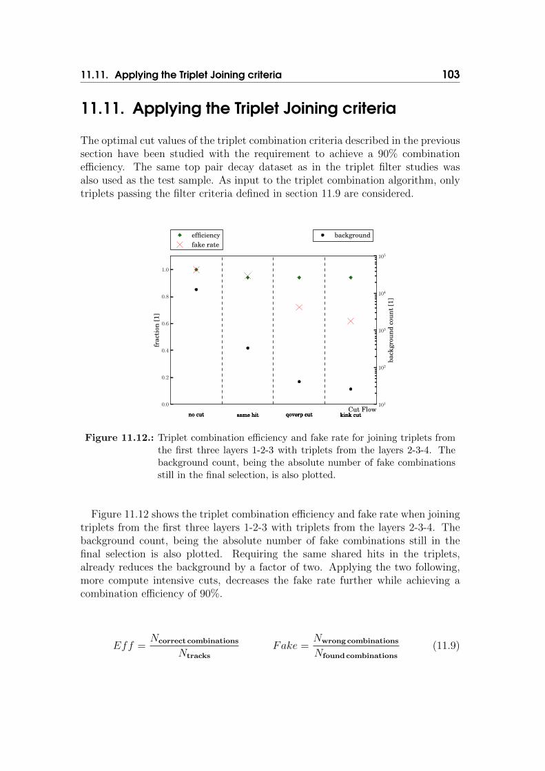
11.11. Applying the Triplet Joining criteria 103
11.11. Applying the Triplet Joining criteria
The optimal cut values of the triplet combination criteria described in the previoussection have been studied with the requirement to achieve a 90% combinationefficiency. The same top pair decay dataset as in the triplet filter studies wasalso used as the test sample. As input to the triplet combination algorithm, onlytriplets passing the filter criteria defined in section 11.9 are considered.
Cut Flow0.0
0.2
0.4
0.6
0.8
1.0
frac
tion
[1]
no cut same hit qoverp cut kink cutno cut same hit qoverp cut kink cut
efficiencyfake rate
101
102
103
104
105
back
grou
ndco
unt
[1]
no cut same hit qoverp cut kink cut
background
Figure 11.12.: Triplet combination efficiency and fake rate for joining triplets fromthe first three layers 1-2-3 with triplets from the layers 2-3-4. Thebackground count, being the absolute number of fake combinationsstill in the final selection, is also plotted.
Figure 11.12 shows the triplet combination efficiency and fake rate when joiningtriplets from the first three layers 1-2-3 with triplets from the layers 2-3-4. Thebackground count, being the absolute number of fake combinations still in thefinal selection is also plotted. Requiring the same shared hits in the triplets,already reduces the background by a factor of two. Applying the two following,more compute intensive cuts, decreases the fake rate further while achieving acombination efficiency of 90%.
Eff =Ncorrect combinations
Ntracks
Fake =Nwrong combinations
Nfoundcombinations
(11.9)

104 Chapter 11. Fast track reconstruction for massively parallel hardware
11.12. Physics results of the OpenCLImplementation
As part of this thesis, the fast triplet finding algorithm described in the previoussections has been implemented using the OpenCL platform and the clever library.
For the following study, two computing platforms will be used to run theOpenCL implementation of the algorithm:
• Classical CPU - Intel Core i7-3930K
This high-end consumer CPU has 6 parallel processing cores which run at3.2 GHz. In the year 2014, this CPU costs around e 500 and provides a peakfloating point performance 154 GFlops.
The operating system Scientific Linux version 6.4 and the Intel OpenCLSDK 2012 was used to run programs on this hardware.
• Consumer GPU - NVIDIA GeForce GTX 660
This GPU is part of a NVIDIA consumer graphics card, costs e 200 in theyear 2014 and offers a peak floating point performance of 1880 GFlops.
The NVIDIA driver version 319.23 was used to provide the OpenCL platformto the programs using this hardware.
The same CPU was also used to execute the default CMS triplet finding algo-rithm, which will be used as a runtime reference. This algorithm is implementedin C++ and runs inside of the CMSSW reconstruction framework. Both CMSSWand the host-side of the OpenCL implementation have been compiled with GCC ver-sion 4.7.2.
Figure 11.13 shows the triplet finding efficiency and fake rate of the algorithmrunning on the NVIDA GPU. The clone rate is the fraction of triplets whichhave been found twice for the same layer combination. This can happen as theindividual detector elements holding the active silicon surface overlap slightlywithin one layer. Therefor, tracks passing in this overlap region, two hits will beproduced in one detector layer. This ambiguity cannot be resolved at the time oftriplet finding but has to be addressed at a later processing stage.
The plot contains entries for each of the studied layer combinations. Forcombinations incorporating hits from strip layers, a higher fake rate can be ob-served. This is due to the previously discussed effects of larger measurement errorand spacing between these layers. The targeted reconstruction efficiency 80% isachieved for all studied layer combinations.
To investigate the triplet finding performance for a varying occupancy of thetracker, a Monte Carlo generated set of muon tracks has been used. Increasingnumbers of tracks have been artificially inserted into one event and handed to theOpenCL triplet finding.

11.12. Physics results of the OpenCL Implementation 105
1-2-3 2-3-4 3-4-5 4-5-8layer triplet
0.0
0.2
0.4
0.6
0.8
1.0fra
ction[1]
tt Simulated Event Studies efficiencyfake rateclone rate
Figure 11.13.: Triplet finding efficiency, fake rate and clone rate of the OpenCLimplementation running on the NVIDA GPU.
100 101 102 103 104
tracks
0.0
0.2
0.4
0.6
0.8
1.0
Physics Performance over Tracks
efficiencyfake rateclone rate
Figure 11.14.: Efficiency, fake rate and clone rate for the triplet finding in the firstthree layers of the detector for an event with one track up to an eventwith 4000 tracks.

106 Chapter 11. Fast track reconstruction for massively parallel hardware
Figure 11.14 displays the efficiency, fake rate and clone rate for the tripletfinding in the first three layers of the detector for an event with one track up toan event with 4000 tracks. The efficiency is stable over the whole range of studiedtracker occupancy, except for the dip at three tracks. In this case, one of the threegenerated tracks is not found and thus affecting the efficiency heavily. As visiblefrom the other efficiency entries, this can be considered to be an outlier.
Also, the fake rate is stable and below 30% for up to one thousand tracks perevent. A sharp increase in fake rate can be observed for even higher occupancies.One way to counter the increase in fake rate in these high-occupancy regimes isto tighten the cuts on triplet candidates and use multiple triplet finding roundsto recover the efficiency losses, very similar to the iterative tracking employed bythe default CMS reconstruction.
The triplet finding algorithm, the cut configuration and the OpenCL implemen-tation running on a GPU have proven to be able to achieve a satisfying reconstruc-tion performance. This demonstrates the feasibility of the proposed approach andshows for the first time, that triplet finding can be performed on CMS input hitson a GPU device.
11.13. Runtime Results of the OpenCLImplementation
In this section, the runtime behaviour of the OpenCL implementation and the de-fault CMS triplet finding will be compared. For the OpenCL-based triplet finding,two hardware backends will also be studied: CPU and GPU. After demonstratingthat a good physics performance can be achieved with GPU-based code, the nextimportant step is to study whether significant gains in runtime can be achieved.
To arrive at a detailed understanding of the runtime performance of variousimplementations, artificially generated events with a varying number of muontracks are used.
Figure 11.15 shows the runtime per event for the OpenCL implementation andthe runtime of the CMSSW triplet finding as reference. For OpenCL, two distinctnumbers are plotted: The wall time reports the time period from starting thecomputation on the host device until the result is available on the host for furtherprocessing. Therefore, the wall time includes the data transfer to the computedevice, the execution of the kernel, and the time to transfer the result data backto the host device’s memory space. In contrast, the kernel time only measuresthe time spent in the actual OpenCL kernels performing the triplet finding.
The CMSSW triplet finding runs solely on the CPU, therefore having no needfor data transfers, only the overall runtime of the computation is plotted. TheCMSSW runtime scales exponentially with a growing number of input tracks,while no pedestal in runtime can be observed for only a few tracks.

11.13. Runtime Results of the OpenCL Implementation 107
10−1
100
101
102
103
104
105
time
/ev
ent[
ms]
Processing Time over Trackswall time GPUkernel time GPU
wall time CPUkernel time CPU
CMSSW 6.0.0
100 101 102 103
tracks / event2−82−62−42−22022242628
ratio
fine grid
Figure 11.15.: Runtime per event for the OpenCL implementation and the runtimeof the CMS triplet finding as reference. The wall time is reportingthe complete processing time, including the OpenCL kernel startupand data transfer, while the kernel time measures only the runtimeof the actual compute kernel.
Both OpenCL platforms, GPU and CPU, behave differently here. For both, aclear pedestal in runtime is observed. This constant overhead is expected, as itis not economical to send very small events, therefore few computations, to theGPU and back.
The more important finding is when, or if at all, this constant overhead can beamortized by a increasing amount of computations on the GPU. Considering onlythe actual runtime of the OpenCL kernel on the GPU, this break-even point isalready reached with 10 track per event. This is for a best-case scenario, where theresults do not need to be copied back to the host memory and further processingcan be performed on the GPU.
In fact, for the OpenCL implementation presented here, the data needs bemoved back to the host side. Including all data transfer and GPU executionoverhead, the GPU implementation outperforms the CPU for around 400 tracksper event.
For the OpenCL-code running on the CPU, a similar constant overhead can beobserved. It is not able to achieve, or surpass, the CMSSW implementation whencomparing the wall time. In fact, only for events with more than 2000 tracks isthe OpenCL CPU version able to achieve a similar performance than CMSSW.
However, for the overall runtime of the GPU implementation a steady gaincompared to the CPU implementations is visible, once the break even point has

108 Chapter 11. Fast track reconstruction for massively parallel hardware
been reached. For events with many tracks, a speedup over the CMSSW imple-mentation of up to a factor of 64 can be observed.
The GPU implementation presented here is able to perform a ten times fastertriplet finding for events with 1000 tracks, which is a realistic number of tracksper event for the upcoming run periods of the LHC.
One way to still amortize for the GPU-induced overhead in less-populated eventsis to bundle many events and send them in one batch to the GPU, process themand return the result.
11.14. Conclusion and Further Steps
The specific challenges in porting HEP reconstruction algorithms to GPU hard-ware have been outlined and the challenges faced by the programmer were iterated.Key features of the clever library, created as part of this thesis work, were ex-plained and it was shown how clever can be used by non-GPU programmingexperts to express data structures, data transfers and algorithms.
Triplet finding and joining algorithms were presented, which have been tailoredto work well on GPU hardware. Cut values to be used by the these algorithmshave been determined by a representative top pair decay dataset. Triplets, whichcombine hits of the barrel tracker layers 1 to 5 and 8, can be reconstructed withan efficiency of 80% and an acceptable fake rate is achieved. In the second stage,triplets from the inner barrel part of the tracker can be combined with an efficiencyof 90%.
The triplet finding algorithm was implemented using OpenCL and the clever li-brary. The physics performance expected from the cut studies is achieved and thereconstruction effiency is stable, even for events with more than 1000 tracks.
For events containing 400 and more tracks, the GPU implementation shows clearruntime improvements with respect to the current, CPU only implementation. Forthe first time in the CMS experiment, part of the event reconstruction has beenported to a GPU target and the physics performance was measured with simulatedevents.
Using the CPU as a platform for OpenCL does not give any benefit. For smallevents with limited complexity, this option is even significantly slower than theC++ implementation of the CMSSW triplet finding algorithm. Therefore, at thepresent time, running OpenCL on CPUs should only be considered as a fallbackoption if no GPU is available on the host machine.
The feasibility of a GPU-based reconstruction has been demonstrated. Simpli-fications of the data structures, a reduction of the geometry detail and tailoredalgorithms were necessary to adapt to the GPU. With careful consideration, re-construction efficiencies comparable with the current, CPU-based reconstructioncan be achieved.

11.14. Conclusion and Further Steps 109
To enable the full track reconstruction on a GPU target, the triplet joiningalgorithm needs to be implemented. The largest work-item here is to implementthe Kalman-filter. The ATLAS experiment has already shown the feasibility ofsuch an implementation on GPUs [96].
Furthermore the integration of a GPU-based track reconstruction into the over-all workflow of the CMSSW framework needs to be studied.


Chapter 12Improving Track Fitting with a detailedMaterial Model
As described in chapter 7.5, a detailed knowledge of the material effects encoun-tered by a particle traversing the detector is necessary to perform a fit of theparticle trajectory.
The CMS track reconstruction employs a material parametrization to estimatethe material effect on a particle trajectory. Therein, for each silicon detectorsurface in the tracker, material constants are stored which represent the mate-rial density around the location of each detector element. In this method, thethree dimensional passive and active material volumes of the tracker material arecondensed onto the two dimensional detector surfaces.
Two parametrized scalar values are available for each detector surface. Theinverse radiation length 1
X0and the material dependant part of the Bethe formula
Xi. These constants have been determined for all detector surfaces in a specialprocedure.
Therein, a Monte Carlo generated sample of neutrinos originating from thedetector center is used. The neutrinos are uniformly distributed in η and φ andcross the detector material with practically no interactions. Still, the knowledgeabout the Geant4 material volumes and detector surfaces they crossed can beused to assign material to specific detector surfaces and compute the two materialconstants.
Once this procedure has been performed for a given detector geometry, thederived material constants can be used to estimate the energy loss and multiplescattering effects on passing tracks in all parts of the tracker.
To compute the energy loss and multiple scattering effects on a track goingfrom detector surface N to surface N + 1, the material constant is looked up forthe detector surface N. Going from surface N + 1 to surface N + 2, the materialconstant from N + 1 is used and so on.
111

112 Chapter 12. Improving Track Fitting with a detailed Material Model
12.1. Limitations of the Current MaterialParametrization
Although the parametrization of the tracker material allows for a fast and reliableestimation of the material effect, there are some simplifications and short-comingsassociated with this method.
As the material constants are linked to the detector surfaces, the actual path ofa specific particle from surface N to N + 1 is not taken into consideration. Whilethis is a valid approximation if the material between layers is equally distributed,it can be an approximation which is too grain in areas with diverse material typesand densities.
Figure 12.1 illustrates this limitation with two tracks originating and arriving atthe same surface but traversing very different material densities. In the parametricapproach, the material effects would be estimated by using an average of bothmaterial densities.
Surface N Surface N+1
Hit iHit i+1
Hit k Hit k+1
DenseMaterial
LightMaterial
Figure 12.1.: Two particle tracks with hits on the same detector surfaces will usethe same material constants in the parametric approximation. In thisdepiction, they cross very different material densities. The parametricenergy loss approximation will use the mean material density of thetransition from surface N to N + 1 in this case.
Furthermore, the parametrization assumes that particle tracks originate fromthe center of the detector. This is true for most tracks, but not for tracks originat-ing from particle decays in secondary vertices. These tracks can originate multiplecentimeters away from the detector center. Many of these signals are important inthe search for possible long-lived SUSY particle candidates or the reconstructionof particle masses, as shown below for the decay of a short-lived kaon.
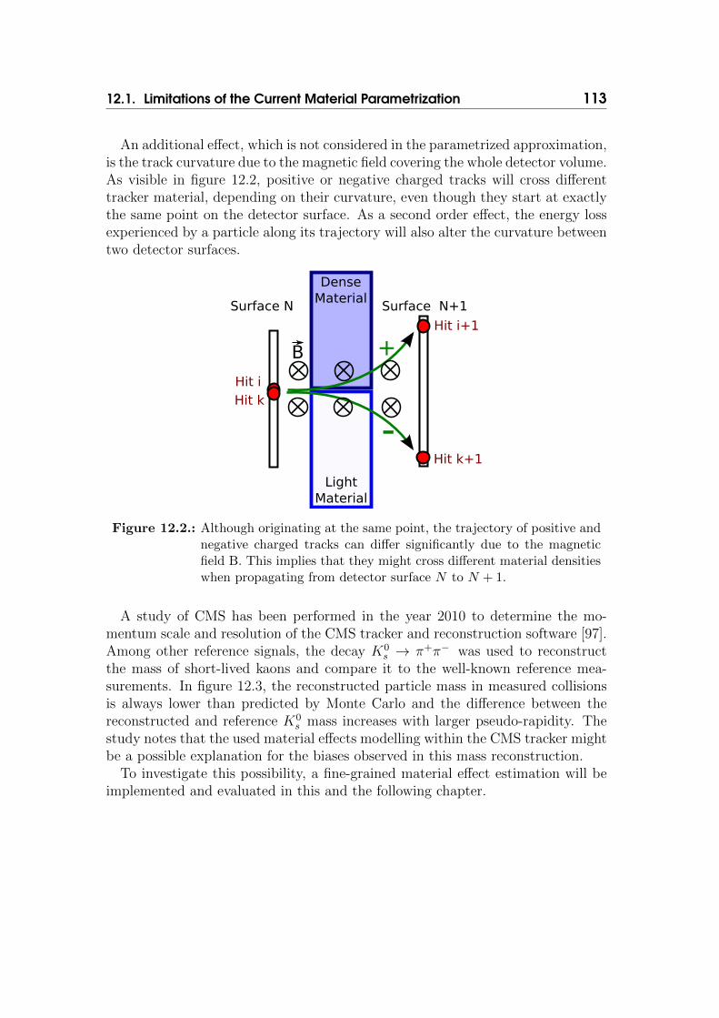
12.1. Limitations of the Current Material Parametrization 113
An additional effect, which is not considered in the parametrized approximation,is the track curvature due to the magnetic field covering the whole detector volume.As visible in figure 12.2, positive or negative charged tracks will cross differenttracker material, depending on their curvature, even though they start at exactlythe same point on the detector surface. As a second order effect, the energy lossexperienced by a particle along its trajectory will also alter the curvature betweentwo detector surfaces.
Surface N Surface N+1
Hit i
Hit i+1
Hit k
Hit k+1
DenseMaterial
LightMaterial
+
-
B
Figure 12.2.: Although originating at the same point, the trajectory of positive andnegative charged tracks can differ significantly due to the magneticfield B. This implies that they might cross different material densitieswhen propagating from detector surface N to N + 1.
A study of CMS has been performed in the year 2010 to determine the mo-mentum scale and resolution of the CMS tracker and reconstruction software [97].Among other reference signals, the decay K0
s → π+π− was used to reconstructthe mass of short-lived kaons and compare it to the well-known reference mea-surements. In figure 12.3, the reconstructed particle mass in measured collisionsis always lower than predicted by Monte Carlo and the difference between thereconstructed and reference K0
s mass increases with larger pseudo-rapidity. Thestudy notes that the used material effects modelling within the CMS tracker mightbe a possible explanation for the biases observed in this mass reconstruction.
To investigate this possibility, a fine-grained material effect estimation will beimplemented and evaluated in this and the following chapter.

114 Chapter 12. Improving Track Fitting with a detailed Material Model
Figure 12.3.: Dependence of the K0s mass on η of the reconstructed kaon. The data
from measured events was recorded with the CMS detector in theyear 2012 at a center-of-mass energy of 7 TeV . A relation between thedetector region where theK0
s was reconstructed and the mass is visible,both in data and simulation. This effect is especially pronounced inthe endcap region [97].

12.2. Geant4 Error Propagation Package 115
12.2. Geant4 Error Propagation Package
The Geant4 error propagation package [98], short Geant4e, is part of the Geant4material simulation software suite and is specifically tailored to the requirementsof track reconstruction.
Geant4e takes the track state and associated error of a particle in the detectoras an input and propagates this state and errors to any target surface. Duringthis procedure, interaction with the tracker material and the magnetic field aretaken into account.
12.3. Energy Loss Validation for the CMS Tracker
To understand the quality of the energy loss approximation, both for the currentmaterial parametrization and the Geant4e method, the predicted energy loss canbe compared to the simulation truth. To this end, Monte Carlo-generated particletracks of muons with a momentum of 1 GeV originating from the detector centerare used to compare the mean energy loss of both methods to the simulation truth.
This comparison can be performed for single propagations when crossing denseregions of the tracker. Furthermore, the energy loss of multiple propagations alongone track can be summed up and the mean energy loss for many tracks in thisregion can be computed.
Figures 12.4a and figure 12.4b show the mean energy loss computed by theregular parametrization method and Geant4e over the whole η range of the tracker.The reference mean energy loss derived from the simulation truth is also displayedin both plots. The mean energy loss estimated by the parametrization methodshows a systematic shift to a higher energy loss for all areas of eta compared tothe reference mean energy loss. When using Geant4e to approximate the meanenergy loss, the result is closer to the simulation truth. The maximum differenceis of the order of 2% in the region η = −2.
Figure 12.5a and figure 12.5b show the approximation for one selected particletransition, passing from the TID to the TEC sub-detector. This region was pickedbecause the amount of material to traverse by the particles is especially high in thisregion, thus affecting the particle trajectory. Due to the geometrical propertiesof the CMS tracker, which can be seen in figure 5.4, the transition of particlesfrom TID to TEC can only occur at a certain band in η, therefore these plots areshowing entries only for the outer η regions.
As visible in figure 12.5a the parametric approach underestimates the meanenergy loss in certain regions of η by more than a factor of 2. The parametricmethod is only able to approximate the mean energy loss in the region around|η| = 1.7 sufficiently well.
In contrast, figure 12.5b shows that the Geant4e method is able to provide a

116 Chapter 12. Improving Track Fitting with a detailed Material Model
η-2.5 -2 -1.5 -1 -0.5 0 0.5 1 1.5 2 2.5
E [
GeV
]∆
Mea
n
0
0.01
0.02
0.03
0.04
0.05
0.06
0.07
0.08
Sim. TruthRegular
Energy Loss in Full Detector
(a) Mean energy loss approximated by theparametrization method and the simu-lation truth.
η-2.5 -2 -1.5 -1 -0.5 0 0.5 1 1.5 2 2.5
E [
GeV
]∆
Mea
n
0
0.01
0.02
0.03
0.04
0.05
0.06
0.07
0.08
Sim. Truth
Geant4e
Energy Loss in Full Detector
(b) Mean energy loss approximated by theGeant4e method and the simulationtruth.
Figure 12.4.: Comparison plots of the parametrization and Geant4e energy loss com-putations for the whole detector.
good approximation of the mean energy loss over the full η range possible for thistransition.
The approximation of the energy loss of individual particles can be validatedfurther by studying the actual energy loss distribution of one individual bin inη. Figure 12.6a and figure 12.6b display the energy loss distribution for the bin−1.8 ≤ η < −1.7 in the transition from the TID to the TEC for the parametricand the Geant4e method, respectively.
A rational function approximating the landau distribution has been fitted tothe histogram of the simulation energy loss using the ROOT package [43] andis overlayed on the histogram. While both the parametric and Geant4e methodshow some discrepancy to the ideal Landau distribution of the energy loss, theGeant4e method performs better.
The backside of the parametric approach becomes especially visible here, as thematerial values are discretized on a per-detector level, the computed energy lossesare concentrated on a few values and the proper shape of the Landau distributionis not approximated properly.
The mean energy loss is not properly modeled by the parametric approach forthis complex transition region of the detector. Although the Geant4e methoddoes not model the Landau tail of the energy loss distribution properly, the meanenergy loss is in good agreement to the values derived from simulation.
Comparisons for all other regions and critical transitions in the CMS tracker
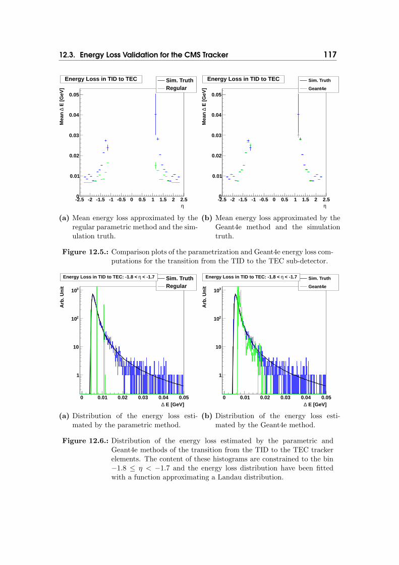
12.3. Energy Loss Validation for the CMS Tracker 117
η-2.5 -2 -1.5 -1 -0.5 0 0.5 1 1.5 2 2.5
E [
GeV
]∆
Mea
n
0
0.01
0.02
0.03
0.04
0.05
Sim. TruthRegular
Energy Loss in TID to TEC
(a) Mean energy loss approximated by theregular parametric method and the sim-ulation truth.
η-2.5 -2 -1.5 -1 -0.5 0 0.5 1 1.5 2 2.5
E [
GeV
]∆
Mea
n
0
0.01
0.02
0.03
0.04
0.05
Sim. Truth
Geant4e
Energy Loss in TID to TEC
(b) Mean energy loss approximated by theGeant4e method and the simulationtruth.
Figure 12.5.: Comparison plots of the parametrization and Geant4e energy loss com-putations for the transition from the TID to the TEC sub-detector.
E [GeV]∆0 0.01 0.02 0.03 0.04 0.05
Arb
. Un
it
1
10
210
310
Sim. TruthRegular
< -1.7ηEnergy Loss in TID to TEC: -1.8 <
(a) Distribution of the energy loss esti-mated by the parametric method.
E [GeV]∆0 0.01 0.02 0.03 0.04 0.05
Arb
. Un
it
1
10
210
310
Sim. Truth
Geant4e
< -1.7ηEnergy Loss in TID to TEC: -1.8 <
(b) Distribution of the energy loss esti-mated by the Geant4e method.
Figure 12.6.: Distribution of the energy loss estimated by the parametric andGeant4e methods of the transition from the TID to the TEC trackerelements. The content of these histograms are constrained to the bin−1.8 ≤ η < −1.7 and the energy loss distribution have been fittedwith a function approximating a Landau distribution.

118 Chapter 12. Improving Track Fitting with a detailed Material Model
have been performed and can be found in appendix C. The parametric approachis able to approximate the mean energy loss over the whole detector fairly well, asvisible in figure 12.4a. In the complex transition region however, the parametricmethod shows significant deficiencies. The Geant4e package is able to achieve agood approximation of the mean energy loss in all parts of the CMS tracker.
12.4. Incorporation of Geant4e in the CMSReconstruction
The CMS reconstruction framework uses abstractions for all functional compo-nents involved in the fitting process. Abstract C++ classes define the interface ofa component and can be inherited to provide a concrete implementation of onepart of the fitting functionalities. Figure 12.7 shows an overview of all componentsinvolved in the trajectory fit.
• KFFittingSmoother
Combines the forward and backward fit of the trajectory to the final result
– KFTrajectoryFitter
Performs the forward fit of the track
∗ Propagator
Propagates track states from hit i to hit i+ 1
∗ KFUpdator
Updates the track state with the current hit i using the Kalmanfilter method
– KFTrajectorySmoother
Performs the backward fit of the track
∗ Propagator
Propagates track states from hit i− 1 to hit i
∗ KFUpdator
Updates the track state with the current hit i using the Kalmanfilter method
Figure 12.7.: Software components involved in the track fit of the CMS reconstruc-tion.
The Propagator interface was used to integrate the Geant4e functionality into

12.4. Incorporation of Geant4e in the CMS Reconstruction 119
the trajectory fitting workflow of CMS. Propagator components take a trajectorystate and a target surface as input values and are responsible for propagatingthe state and associated errors to the target surface. The trajectory state andthe associated error matrix is returned to the calling program code. If the targetsurface cannot be reached, for example due to curling trajectories in the magneticfield, an invalid trajectory is returned.
Propagators support two modes of operation: forward and backward propaga-tion. During forward propagation, the particle is propagated along its trajectory,starting from hit n and arriving at the next hit n + 1. In contrast, during back-ward propagation mode, the trajectory of the particle is followed in the oppositedirection. Here, the propagation starts at hit n and arrives at the previous hitn − 1. Even if the backward mode does not reflect the travel direction of theparticle, it is needed for the smoothing step of the Kalman filter.
After the backward propagation, the particle has gained energy along its tra-jectory. Furthermore, the particle charge has to be inverted so the influence ofthe magnetic field on the trajectory is consistent between forward and backwardpropagation. Both propagation modes are used during the trajectory fit.
Multiple Propagator implementations exist in the CMSSW code base. Someare intended for fast execution and assume the particle travels on a perfect helix,while others provide a more fine-grained approximation of the magnetic field andmaterial effects.
For the default track fitting of CMS, a Runge-Kutta based method is used tocompute the propagation of the particle in the magnetic field and the aforemen-tioned parametric method is employed to compute the material effects, namelymultiple scattering and energy loss, on the particle trajectory.
A Geant4ePropagator class has existed in the CMS code base for many years,but has never been successfully used for the final trajectory fit. It converts thetrack state and associated errors from the representation used by CMS to the oneused by Geant4. Furthermore, it defines the so-called target surface to Geant4e.This a virtual plane in 3d space within the detector volume to which the state ofthe particle must be propagated. For a track propagation from detector surfaceN to N + 1, the target surface will be aligned with the active silicon plane of thedetector N + 1.
During the regular CMS reconstruction setup, only a slimmed down geome-try of the tracking system is available to the modules. This geometry containsonly the active Silicon surfaces and their location and rotation in space. TheGeant4ePropagator needs a more detailed information about the geometry, espe-cially also about the passive volumes. Therefore, the Geant4 geometry is loadedbefore the reconstruction job is started using a special GeometryProducer. Fur-thermore, the magnetic field representation of Geant4 is loaded by the Geome-tryProducer.
In addition to the functionalities already provided by the Geant4ePropagator, a

120 Chapter 12. Improving Track Fitting with a detailed Material Model
range of additional features were implemented as part of this thesis to successfullyperform a full trajectory fit:
• Error deflation in backward mode
While the errors on the track parameters are inflated during the forwardpropagation, they have to be deflated during the backward propagation.Geant4e must be instructed explicitly to perform the error deflation. Thiscan be done via the method call:
1 G4ErrorPropagatorData : : SetStage ( G4ErrorStage stage )
This method can either be called with G4ErrorStage Inflation orG4ErrorStage Deflation to set the handling of the error during the prop-agation.
• Unit conversion
The internal units of CMS are cm for length and GeV for energies. In con-trast, Geant4 uses mm and MeV for length and energies, respectively. There-fore, all conversions of track parameters and error matrices between CMSand Geant4 need to take the different units of the two software packagesinto consideration.
Missing unit conversions have been added to the Geant4ePropagator toachieve a consistent data exchange between the two software packages.
• Path length convention
The path length of the propagation can be queried from Geant4e once thepropagation is complete. Herein, Geant4e will always return a positive pathlength, also for backward propagations. The CMS convention however is,that a backward propagation must result in a negative path length value.To comply with this convention, the Geant4ePropagator was changed toprovide a positive or negative signed path length to the CMS reconstruction,depending on the propagation direction.
Furthermore, a programming error in the Geant4 package was discovered duringthe integration with CMSSW. This software bug, called a memory leak, causedGeant4e to allocate unnecessary amounts of memory for each track propagationand prevented the processing of more than 1000 tracks due to the system run-ning out of free memory. A bug fix was provided to the Geant4 developmentteam [99] which corrects the copious memory usage. As a positive side effect ofthis correction, the overall runtime of the propagation step decreased by a factorof 4 [99].

12.5. Fitting of Muon Trajectories 121
The provided bug fix was integrated into the official Geant4 release and allexperiments using the Geant4e propagation can now benefit from the improvedmemory and runtime behaviour of the application.
12.5. Fitting of Muon Trajectories
As a first application of track fits with Geant4e, Monte Carlo generated muonshave been used. These particles originate at the center of the detector and theirdirection is equally distributed in φ and the η range η = [−2.5, 2.5], exactly thecoverage of the CMS tracker. The transverse momentum pT of the muon particlesis equally distributed between [0.9, 1.1] GeV as particles in this low transversemomentum range are most heavily affected by energy loss in the detector. Half ofthe muons have a positive charge, while the other half has a negative charge.
The tracks of the particles have been fitted with the parametric material esti-mation and the Geant4e method.
The first quality criteria which will be studied are the pull distributions of thefitted parameters. Overall, five parameters are fitted with the Kalman method asintroduced in section 7.3. The pull of the fit parameter T can be computed usingthe formula:
p(T ) =Treco − Tsim
σT
Herein, Treco is the parameters value provided by the reconstruction, Tsim is thetrue value known from the simulation and σT is the error on the reconstructedvalue. The pull distribution resulting from computing the above formula for manyfitted parameters allows to evaluate a possible bias of the reconstruction andalso whether the uncertainties on the reconstructed parameters are under- oroverestimated.
Figure 12.8a shows the pull distribution of the regular, parametric fit methodfor the fit parameter 1/p while figure 12.8b shows the same distribution for theGeant4e-based fit method.
A gaussian function has been fitted to both distributions and the resulting meanand sigma can be used to evaluate the quality of the track fitting procedure.
Furthermore, figures 12.9a and 12.9b show the pull distributions for the para-metric and Geant4e-based fits for the θ fit parameter. A similar trend as in the1/p pull distributions is visible here: the Geant4e-based method is able to achieveslight improvements both for the mean values of the pull distribution as well asfor the width.
As described in chapter 5, the CMS tracker has very different material densitiesand types at various locations along the particle trajectory. Therefore, it is alsoof interest to study the fitting performance along various parts of the detector.

122 Chapter 12. Improving Track Fitting with a detailed Material Model
Pull of 1/p-5 -4 -3 -2 -1 0 1 2 3 4 50
2000
4000
6000
8000
10000
12000
14000
16000
18000
20000
22000
24000
^2 / N = 9.08e+03 / 97 = 93.6χ 0.001436± = 0.07722 µ
0.0012± = 1.111 σ
(a) 1/p pull distribution of the parametricmethod.
Pull of 1/p-5 -4 -3 -2 -1 0 1 2 3 4 50
5000
10000
15000
20000
25000^2 / N = 5.26e+03 / 97 = 54.3χ
0.001387± = -0.005745 µ
0.001127± = 1.089 σ
(b) 1/p pull distribution of the Geant4emethod.
Figure 12.8.: Pull distributions of the fit parameter 1/p for the parametric andGeant4e methods.
θPull of -5 -4 -3 -2 -1 0 1 2 3 4 50
5000
10000
15000
20000
25000
30000
^2 / N = 2.22e+04 / 97 = 229χ 0.001191± = 0.001946 µ
0.001166± = 0.9264 σ
(a) Pull of θ distribution of the parametricmethod.
θPull of -5 -4 -3 -2 -1 0 1 2 3 4 50
5000
10000
15000
20000
25000
^2 / N = 7.22e+03 / 97 = 74.4χ 0.001247± = 0.001426 µ
0.001047± = 0.9834 σ
(b) Pull of θ distribution of the Geant4emethod.
Figure 12.9.: Pull distributions of the fit parameter θ for the parametric andGeant4e methods.

12.5. Fitting of Muon Trajectories 123
(a) Residual of the 1/pT value when fittingall track hits with the parametric andGeant4e methods.
(b) Residual of the 1/pT value when fit-ting only the strip detector hits withthe parametric and Geant4e methods.
Figure 12.10.: Residual of the 1/pT value for various bins in η when using either allavailable hits of the track (left), or only the hits in the strip tracker(right). Note the different scale of the y-axis between the plots.
The mean residual of the fitted inverse transverse momentum parameter:
res(pT) =1
pTreco− 1
pTsim
plotted over η is displayed in figure 12.10a. The improvements in the barrelregion are visible when using the Geant4e-method compared to the parametricmethod. In the transition and endcap region of the tracker, starting at |η| ≈ 0.7the Geant4e-method shows clear improvements. The residuals in the outer binsof η are closer to zero and overall show a much flatter behaviour.
Figure 12.11b shows the distribution of the residuals over η in case only hitsfrom silicon strip detectors are used. Therefore, the fit will be performed withoutthe two to four pixel hits in the center of the tracker. Fits with missing pixel hitsare necessary to reconstruct particles from secondary vertices which are outsideof the last pixel layer or cosmic muon tracks which enter the detector from theoutside and do not necessarily cross the pixel tracker volume.
In this scenario, the performance of the Geant4e-method is significantly better.The bias in the barrel region of the parametric method cannot be observed withGeant4e. While the residual in the endcap worsens considerably for the parametricmethod, the Geant4e-methode is able to maintain the smaller residual already seenin the fit with all tracker hits.

124 Chapter 12. Improving Track Fitting with a detailed Material Model
η-2.5 -2 -1.5 -1 -0.5 0 0.5 1 1.5 2 2.5
[GeV
]ptσ
0
0.01
0.02
0.03
0.04
0.05
Parametric
Geant4e
(a) Sigma of the transverse momentummeasurement when fitting all track hitswith the parametric and Geant4e meth-ods.
η-2.5 -2 -1.5 -1 -0.5 0 0.5 1 1.5 2 2.5
[GeV
]ptσ
0
0.01
0.02
0.03
0.04
0.05
Parametric
Geant4e
(b) Sigma of the transverse momentummeasurement when fitting only thestrip detector hits of the track with theparametric and Geant4e methods.
Figure 12.11.: Sigma of the transverse momentum measurement for various bins inη when using either all tracker hits (left), or only the hits in the striptracker (right).
Figures 12.11a and 12.11b show the measurement error on pT as returned bythe track fit for all hits and the fit with strip hits-only, respectively. The plotsshow, that the error on the reconstructed pT is slightly smaller, especially in theendcaps, when using the Geant4e-method compared to the parametric one. Asexpected, the error of the strip hits-only fit is larger, as fewer measurement pointswere included in the track fit.

Chapter 13Reconstruction of the short-lived KaonMass
The copious production of kaons in the pp-collisions delivered by the LHC machineallows to use the decay of these particles as a reference for the evaluation ofreconstruction algorithms. The well-known reference mass of the kaon can becompared with the mass resulting from the event reconstruction in simulated andmeasured events. Especially interesting for track reconstruction validation is thedecay of the short-lived kaon K0
s . Table 13.1 lists the hadronic decay modes ofthe K0
s into either two pions of neutral charge, two pions of opposite charge ortwo pions of opposite charge and one neutral pion.
Table 13.1.: Branching fractions of the hadronic decays of the short-lived kaonK0s [4].
Decay Mode Branching Fraction Γi/ΓK0s → π0π0 30.69
K0s → π+π− 69.20
K0s → π+π−π0 3.5 · 10−7
Apart from the highly suppressed decay K0s → π+π−π0, the decay K0
s → π+π−
is the only one which can be reconstructed solely based on tracker information.
The mass of the K0s particle is mK0
s= 497.614 ± 0.024 MeV according to the
fit of the Review of Particle Physics publication, which combines the measuredresults from multiple experiments [4]. This value will be used in the following asthe K0
s mass reference.
125

126 Chapter 13. Reconstruction of the short-lived Kaon Mass
13.1. K0s Detection and Reconstruction
The decay of a K0s particle leaves a distinct signature in the tracker: two tracks
with opposite charge emerge from a displaced vertex. Due to the K0s being neutral,
no single track leads to this secondary vertex.A range of cuts have been applied to the reconstructed particle tracks to identify
possible K0s decays [100]:
• The normalized χ2 value of the track fit must be 5 or better
• The number of valid hits on one track must be 6 or higher
All tracks passing these initial quality criteria are evaluated in pairs of oppositecharge combinations. Between each of the possible combinations, the point ofclosest approach between the tracks is computed. Two cuts are applied to reducethe candidate combinations:
• The mass of the di-pion system must be smaller than 0.6 GeV
• The closest distance between the tracks must be smaller than 1 cm
All track combinations which pass these criteria are used as input to a vertexfit. Once this fit has been performed, the position and associated errors for apossible secondary vertex have been computed and additional quality cuts can beapplied:
• The normalized χ2 of the vertex fit must be 7 or smaller
• The innermost hits on both tracks originating from the secondary vertexmust not be closer to the beam spot than 4 sigma of the radial vertexposition. This helps to ensure that the two tracks actually originate fromthe secondary vertex and do not stem from another primary vertex at thebeam spot
• The reconstructed mass at the secondary vertex must lie between ±70 MeVof the K0
s reference mass as listed by the PDG [4]
13.2. DatasetFor the following study, simulated collision events and data recorded by the CMSdetector will be used. The simulated collisions have been generated at a center-of-mass energy of
√s = 8 TeV using the Pythia6 [44] event generator with the
Z2star tune [101]. The decay and the interaction of the generated particles withthe detector were simulated using the Geant4 package.

13.2. Dataset 127
The data presented here was recorded by the CMS detector at a center-of-massenergy of
√s = 8 TeV at the beginning of the year 2012.
Both, simulated and recorded events, have been reconstructed using the CMSreconstruction and K0
s decay candidates have been identified using the techniquedescribed above.
Number of Primary Vertices0 5 10 15 20 25 30 35
a.u.
0
0.02
0.04
0.06
0.08
0.1
Simulation
Data
= 8 TeVs
Figure 13.1.: Number of primary vertices (NPV) in recorded and simulated events.The simulated events have been reweighted to fit the NPV distributionobserved in recorded events.
Figure 13.1 shows the distribution of the number of primary vertices (NPV),both in the recorded and simulated events with the average number being 11 inthe recorded events. The simulated events have been reweighted so their NPV-distribution corresponds to the one observed in data.
The position of the decay vertex of the K0s in radial and Z-direction is shown
in figures 13.2a and 13.2b. This information has been retrieved from simulationtruth and therefore shows the decay position independent of the employed recon-struction technique. The most kaons decay close to the interaction point, but asignificant amount of decays take place outside of the pixel tracker at R > 12 cmand |Z| > 50 cm.
Only a part of the pion tracks resulting from the K0s decays leave sufficient hits
in the tracking system to allow for a detection and reconstruction of the decay.As described in chapter 7, tracks can only be found if sufficient hits exist in theinner tracking system to allow for an initial seeding of the track. Therefore, atleast two properly measured hits on each of the pion tracks are required to findthese tracks and in turn reconstruct the decay vertex of the K0
s . As the seedingis performed in the most precise, innermost layers of the tracker, highly displacedvertices are less likely to be detected.

128 Chapter 13. Reconstruction of the short-lived Kaon Mass
Secondary Vertex R [cm]0 20 40 60 80 100
a.u.
0
0.01
0.02
0.03
0.04
0.05
0.06
= 8 TeVs
(a) Radial position of the K0s decay vertex.
Secondary Vertex Z [cm]-100 -50 0 50 100
a.u.
0
0.01
0.02
0.03
0.04
0.05
0.06
= 8 TeVs
(b) Z position of the K0s decay vertex.
Figure 13.2.: Decay position of the K0s in relation to the interaction point. This
location has been retrieved from simulation truth.
Reconstructed Secondary Vertex R [cm]0 20 40 60 80 100
a.u.
0
0.01
0.02
0.03
0.04
0.05
0.06
0.07
0.08
0.09 Simulation
Data
= 8 TeVs
(a) Radial position of the K0s decay vertex.
Reconstructed Secondary Vertex Z [cm]-100 -50 0 50 100
a.u.
0
0.01
0.02
0.03
0.04
0.05
0.06
0.07
0.08
Simulation
Data
= 8 TeVs
(b) Z position of the K0s decay vertex.
Figure 13.3.: Reconstructed location of the K0s decay vertex position in simulated
and recorded events.

13.2. Dataset 129
+ Pt [GeV]π0 2 4 6 8 10
a.u.
-810
-710
-610
-510
-410
-310
-210
-110Simulation
Data
= 8 TeVs
(a) Positive charged pions originating fromthe K0
s decay.
- Pt [GeV]π0 2 4 6 8 10
a.u.
-810
-710
-610
-510
-410
-310
-210
-110
Simulation
Data
= 8 TeVs
(b) Negative charged pions originatingfrom the K0
s decay.
Figure 13.4.: Transverse momentum spectra of the positive and negative chargeddaughter pions used to reconstruct the short-lived kaon.
Figures 13.3a and 13.3b show the distribution of the K0s decay location pro-
vided by the event reconstruction using the technique described in section 13.1for both simulated and recorded events. The location of the reconstructed verticesis consistent between both datasets. The decrease of found decays with increas-ing distance from the interaction point is visible in both plots with virtually noreconstructed decays outside of R > 55 cm and |Z| > 60 cm. Increases in the effi-ciency are visible in the plot 13.3b the positions |Z| = 34.5 cm and |Z| = 46.5 cm.These are effects introduced by an interplay between the tracker layout and thereconstruction algorithm. Four layers of detection elements of the forward pixeldetector are located at |Z| = 34.5 cm and |Z| = 46.5 cm on both sides of theinteraction point. The additional measurement points provided by the layers atthese locations enable the vertex finding to achieve a better, though very localized,increase of the efficiency.
Figures 13.4a and 13.4b show the distributions of the transverse momentum(pT) of the positive and negative charged pions which are used to reconstruct theK0s mass. Both plots show, that the pT spectrum in data is harder, meaning more
high energetic pion tracks have been reconstructed in recorded events as in thesimulation.
As expected, this observation is also visible in figure 13.5, which shows thetransverse momentum of the K0
s reconstructed from the two pion tracks.These discrepancies in the momentum distribution can either be a result of im-
perfections in the modelling of the Pythia6 Monte Carlo generator or an artifact

130 Chapter 13. Reconstruction of the short-lived Kaon Mass
Kaon Pt [GeV]0 2 4 6 8 10
a.u.
-610
-510
-410
-310
-210
-110Simulation
Data
= 8 TeVs
Figure 13.5.: Transverse momentum distribution of the K0s reconstructed from two
pion daughter particles.
of the slight differences in the reconstruction efficiencies between simulated andmeasured events. For the following study, no correction to the simulated spec-trum will be applied, as simulated and measured events will always be treatedseparate and the absolute transverse momentum of both will not enter into thesame computations.
13.3. Mass ReconstructionThe reconstructed mass of each individual kaon decay is collected in a histogramand can be used to derive the invariant mass of the particle. The K0
s mass spec-trum was measured differently either in bins of pseudo-rapidity η, the transversemomentum of the K0
s or the average transverse momentum of the pions.
Dpeak(x) = g ∗ exp(−1
2(x− µσ
)2) (13.1)
Dbkg(x) = a+ bx+ cx2 (13.2)
D(x) = Dpeak +Dbkg (13.3)
Each of these distributions is fitted with equation 13.3, which combines modelsof the decay peak and background distribution of the reconstructed particle decay.The mass peak of the K0
s decay is modeled as a Gaussian function, listed inequation 13.1, and the mean µ of the fitted Gaussian function is used as anestimator for the kaon invariant mass in this specific bin. The σ parameter of

13.3. Mass Reconstruction 131
mass [GeV]sK0.44 0.46 0.48 0.5 0.52 0.54 0.56
Eve
nts
/ 1 M
eV
0
200
400
600
800
1000
1200
= 8 TeVs
(a) Central barrel bin 0.0 < η < 0.25.
mass [GeV]sK0.44 0.46 0.48 0.5 0.52 0.54 0.56
Eve
nts
/ 1 M
eV
100
200
300
400
500
600
= 8 TeVs
(b) Endcap bin 2.0 < η < 2.25.
Figure 13.6.: Distribution of the K0s mass for a central barrel and endcap bin. Both
mass distributions have been fitted with function 13.3, a gaussian func-tion to match the signal peak and a quadratic polynomial to modelthe background.
the Gaussian function can be used to estimate the reconstruction resolution ofthe invariant mass. Equation 13.2 is a quadratic polynomial and is used to modelbackground contribution to the histogram.
The same modelling method has been used in the CMS publication [97] wherethe previous studies on the K0
s mass reconstruction in various η bins have beenperformed and resulted in the plot shown in figure 12.3. Using the same methodin this study allows to perform a direct comparison of the results.
Figure 13.6a shows the distribution of the reconstructed K0s mass from mea-
sured data for an η bin in the central barrel part of the detector. The histogramentries are overlayed with the result of fitting function 13.3 to the distribution.Figure 13.6b shows the same type of plot for a η bin in the endcap area of thedetector. It can be observed from these plots, that the background contributionin the endcap region is more pronounced and also the width of the decay peak iswider in the endcap area.
As both plots show, the fitted function 13.3 is able to model the observed distri-butions, both in the central barrel and endcap region, properly. The distributionsand mass fits for all η bins are listed in appendix D.
Figure 13.7 presents all mass fits for simulated events of the individual η binsover the whole acceptance range of the CMS Tracker. The red entries, labeled“Regular”, are the result of the regular reconstruction using the parametric mate-rial estimation. The blue entries, labeled “Geant4e” show the reconstructed mass

132 Chapter 13. Reconstruction of the short-lived Kaon Mass
η sK-3 -2 -1 0 1 2 3
mas
s [G
eV]
sK
0.495
0.496
0.497
0.498
0.499
0.5
0.501 Regular
Geant4e
= 8 TeVs
Figure 13.7.: Reconstructed K0s mass in η-bins for the regular reconstruction and
the uncorrected Geant4e reconstruction. The black dotted line marksthe reference mass of the K0
s of the Particle Data Group [4].
when using Geant4e during the track fit of the K0s reconstruction. The black
dotted line marks the reference mass of the K0s .
The Geant4e-based fit is able to reconstruct the K0s mass with a smaller fluc-
tuation between the η bins than the regular method. Especially in the endcaps,the changes in mass between the different bins in η are smaller. While the regularmethod is slightly overestimating the K0
s mass, the Geant4e-based fit systemati-cally underestimates the mass.
As figure 13.7 is purely based on simulated events, the same Geant4 materialhas been used to simulate and reconstruct the events. One naively expects theGeant4e-method to achieve a flat distribution over η and to match the K0
s masscorrectly.
However, the material maps in the parametric method have been calibrated onknown resonance peaks, like the K0
s decay, in measured events to achieve the bestpossible performance in the reconstruction of recorded data. This allows for a freeparameter, the overall scale of the track momentum in the reconstruction, to beadjusted to achieve the correct scale on measured data.
pcorr = c ∗ puncorr (13.4)
To also account for this momentum scale parameter, a similar technique hasbeen applied to the Geant4e-method to achieve the correct momentum scale.The momentum of the pion tracks have be multiplied by the factors 0.01, 0.05and 0.005 and the average K0
s mass for all bins in η has been computed. Withthe constraint that the average K0
s mass must be the reference value of mK0s
=

13.3. Mass Reconstruction 133
497.614± 0.024 MeV. An interpolation between the tested correction factors wasperformed and the optimal correction factor to achieve the K0
s reference mass onaverage was determined to:
c = 1.001294
Figure 13.8.: Reconstructed K0s mass in η-bins for the regular reconstruction and
the corrected Geant4e reconstruction, with a momentum correction ofc = 1.001294 applied.
Figure 13.8 shows the reconstructed K0s mass with the momentum scale cor-
rection applied to the Geant4e-fitted tracks. As expected, the correction shiftsthe reconstructed mass on top of the reference mass. A non-flat structure in ηis still visible for the Geant4e-based reconstruction. This is especially visible inthe endcap, where also the statistical error bars are larger, due to the wider re-construction resolution. However, for all η bins, except for the one at η = −1.4,the Geant4e method is able to achieve a better compatibility with the referenceK0s mass than the the regular fit method does. This improvement is especially
visible in the endcap regions for |η| > 1.4.Figures 13.9a and 13.9b show the reconstruction resolution of the K0
s masspeak of the regular method and the scale-corrected Geant4e-method. Figure 13.9bshows the resolution of these two methods over φ of the reconstructed K0
s . Whilea slight decrease of the resolution in the regions around |φ| = −2 is visible forboth methods, the Geant4e-method is able to achieve a better resolution, about4% on average.
Figure 13.9a, which shows the resolution plotted over η, a small improvementwhen using Geant4e is visible over the whole η range. Especially in the threeoutermost bins of the endcap the improvement is most pronounced.
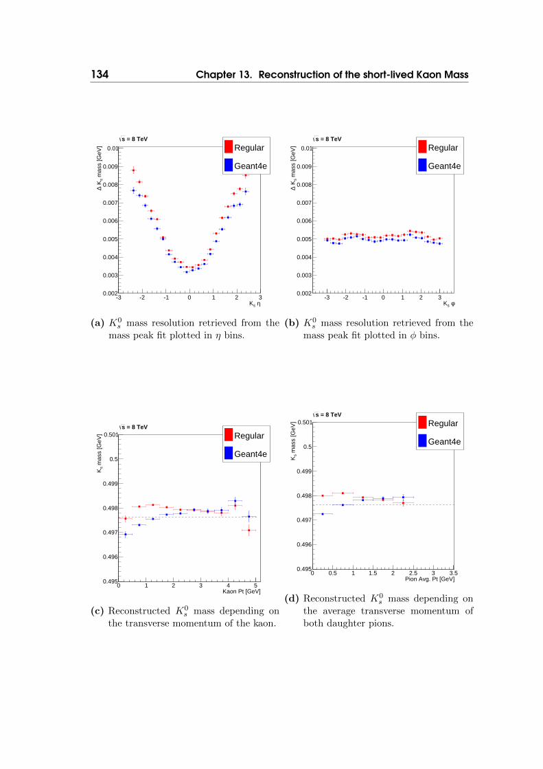
134 Chapter 13. Reconstruction of the short-lived Kaon Mass
η sK-3 -2 -1 0 1 2 3
mas
s [G
eV]
s K∆
0.002
0.003
0.004
0.005
0.006
0.007
0.008
0.009
0.01 Regular
Geant4e
= 8 TeVs
(a) K0s mass resolution retrieved from the
mass peak fit plotted in η bins.
φ sK-3 -2 -1 0 1 2 3
mas
s [G
eV]
s K∆
0.002
0.003
0.004
0.005
0.006
0.007
0.008
0.009
0.01 Regular
Geant4e
= 8 TeVs
(b) K0s mass resolution retrieved from the
mass peak fit plotted in φ bins.
Kaon Pt [GeV]0 1 2 3 4 5
mas
s [G
eV]
sK
0.495
0.496
0.497
0.498
0.499
0.5
0.501 Regular
Geant4e
= 8 TeVs
(c) Reconstructed K0s mass depending on
the transverse momentum of the kaon.
Pion Avg. Pt [GeV]0 0.5 1 1.5 2 2.5 3 3.5
mas
s [G
eV]
sK
0.495
0.496
0.497
0.498
0.499
0.5
0.501 Regular
Geant4e
= 8 TeVs
(d) Reconstructed K0s mass depending on
the average transverse momentum ofboth daughter pions.

13.4. Reconstruction Performance in Specfic Detector Regions 135
Figures 13.9c and 13.9d display the reconstructed K0s mass in relation to the
transverse momentum of the kaon and average pion pT, respectively. A dependenceof the reconstructed K0
s mass on the transverse momentum is visible for bothreconstruction methods, although the shape of the dependence is different in theregion pT < 2GeV.
13.4. Reconstruction Performance in SpecficDetector Regions
(e) Reconstructed K0s mass distribution if
at least one of the two daughter pionsis located in the region 1.5 < η < 1.75.
(f) Reconstructed K0s mass distribution if
at least one of the two daughter pions islocated in the region 2.25 < η < 2.5.
Figure 13.9.: Reconstructed K0s mass distribution of the regular and Geant4e fit-
ting methods for two detector regions with challenging material dis-tributions. The black dotted line indicates the reference mass of theK0s particle. Equation 13.3 has been fitted to both distributions and
the resulting mass is drawn as red and blue lines for the regular andthe Geant4e reconstruction, respectively.
As described in chapter 5, the transition and endcap regions of the CMS trackerhave a larger material budget as the central barrel region. Therefore, improve-ments to the reconstruction material model can be expected to be most pro-nounced in these regions. In fact, the investigation on muon tracks and the re-constructed K0
s mass presented in this and the previous chapter have shown thebiggest improvements in the transition and endcap regions.

136 Chapter 13. Reconstruction of the short-lived Kaon Mass
To study the magnitude of possible improvements in detail, K0s decays have
been selected where at least one of the daughter pion tracks is located in material-dense η regions of the tracker. Figure 13.9e presents distributions of the recon-structed K0
s mass for the regular and Geant4e methods in the transition region1.5 < η < 1.75 where the radiation length x/X0 is the largest. Both distributionshave been fitted with equation 13.3 and the resulting K0
s mass is drawn as redand blue lines for the regular and the Geant4e reconstruction, respectively. Thereference K0
s mass is plotted as a black line. Figure 13.9f shows the same type ofplot, but requiring at least one of the daughter pion tracks in the endcap regionof 2.25 < η < 2.5.
Table 13.2.: Reconstructed K0s masses using the regular and Geant4e methods in
the transition and endcap region. The relative and absolute differenceof the resluting K0
s masses compared to the reference mass is also listed.
1.5 < η < 1.75 1.5 < η < 1.75Regular MethodK0s mass [MeV] 498.78± 0.07 499.3± 0.1
Abs. diff to ref. [MeV] 1.7 1.69Rel. diff to ref. [%] 0.25 0.34Geant4e MethodK0s mass [MeV] 497.54± 0.05 497.5± 0.1
Abs. diff to ref. [MeV] 0.047 0.11Rel. diff to ref. [%] 0.015 0.015
Table 13.2 lists the reconstructed K0s masses for the two methods and the abso-
lute and relative difference to the referenceK0s massmK0
s= 497.614± 0.024 MeV[4].
In both studied regions, transition and endcap of the tracker, a significant im-provement of the K0
s mass reconstruction when using the Geant4e method isvisible. The regular material method results in a systematic shift of the mass dis-tribution to higher masses, which cannot be observed with the Geant4e method.The K0
s mass reconstructed with the Geant4e method is compatible within theerrors with the reference value while the result of the regular reconstruction isnot.
13.5. Mass Reconstruction of Measured EventsThe next logical step is to evaluate the performance of the Geant4e-based track re-construction on events recorded with the detector. Figure 13.10 shows theK0
s massreconstruction using the Geant4e-method both on simulated and measured events.

13.6. Conclusion and Future Steps 137
Figure 13.10.: Reconstructed K0s mass using the Geant4e material model for simu-
lated and real events.
The momentum scale correction derived in the previous section has been appliedto both.
Employing the Geant4e-method results in a reconstructed K0s mass which is
systematically below the reference value. Additionally, the reconstructed mass inmeasured events diverts stronger from the reference mass as in simulation.
13.6. Conclusion and Future Steps
In this chapter, the mass reconstruction of the short-lived kaon K0s was employed
to validate the performance of the Geant4e-based track reconstruction.
For simulated events, a global momentum scale correction has been derived.After applying this correction, the new fitting method shows improvements inthe reconstruction of the K0
s mass in the barrel region, but enhancements areespecially visible in the endcap region. Also a slight resolution improvement ofthe reconstructed mass peak can be observed.
This improved performance cannot be achieved when using the Geant4e-methodon events measured with the CMS detector in the year 2012. The reconstructedmass is systematically lower than the K0
s reference mass. One possible explana-tion for this result is the discrepancy between the Geant4 geometry setup andthe actual material present in the detector. This implies, that the current Geant4detector model is not sufficiently precise to achieve an improvement in the recon-struction performance in measured events.
The Geant4e-method developed as part of this thesis allows to improve this

138 Chapter 13. Reconstruction of the short-lived Kaon Mass
Geant4 geometry to better reflect the actual material distribution within thedetector. For the first time in CMS, particle tracks were fitted using the fullGeant4 material estimation and detailed comparisons between simulated and re-constructed tracks were performed. Eventually, insights gained with these kindof studies can be fed back to the Geant4 detector model to improve the overallquality of simulated events in the CMS detector.
As shown in this chapter, the reconstruction performance of particle masses canbe improved with the Geant4e method if a sufficiently precise Geant4 geometrymodel of the detector is available. Also, decay products in the endcap region canbe more precisely reconstructed.
This allows to better reconstruct complex particle decays, where at least onedecay product trajectory is located in an endcap region.

Chapter 14Conclusion and Outlook
The first part of this thesis focused on improving the processing speed of HEPapplications by making better use of the vector units in modern CPUs. Existingimplementations can be adapted and auto-vectorized using modern C++ compil-ers. Furthermore, the vdt library, which has been developed and evaluated as partof this work, speeds up the computation of mathematical functions in simulationand reconstruction software.
Both techniques have been applied to the CMS reconstruction to improve theruntime performance of the vertex finding, resulting in a speedup of more thana factor 2. The improved version of this algorithm has been successfully usedto reconstruct the events recorded during the 2012 data taking, which led to theannouncement of the Higgs boson discovery in July 2014.
The application of auto-vectorization significantly widens the physics reach ofcurrent and future experiments by the ability to increase the number of processedmeasurements and thus study more rare processes. Future software designs forevent simulation and reconstruction applications need to consider the vectorizedprocessing of data in order to fully utilize the hardware capabilities of today andtomorrow.
The vdt library is now available open-source and royalty-free to allow otherphysics experiments to benefit from the collection of fast and vectorized mathe-matical functions. The Geant4 material simulation package uses the vdt libraryin its most recent release version 10 to improve the runtime of the application.Furthermore, vdt has been integrated into the ROOT data analysis framework.
To cope with the increased amount of recorded data expected during the up-coming years of the LHC, the parallel computing power of GPUs are a promisinghardware option and complements the use of vector units in classical CPUs. Inorder to port the CMS track reconstruction to GPU accelerators, the algorithmsneed to be adapted to the differing memory layout and massive parallelism pro-vided by this hardware. As part of this thesis, algorithms have been developed
139
140 Chapter 14. Conclusion and Outlook
which can perform well with single-precision floating point data and provide ahigh level of parallelism within the processing of one event.
Triplet finding and joining algorithms were presented, which have been tailoredto work well on GPU hardware. Cut values to be used by these algorithms havebeen determined by a representative top pair decay dataset. Triplets, which com-bine hits of the barrel tracker layers 1 to 5 and 8, can be reconstructed with anefficiency of 80% and an acceptable fake rate. In the second stage, triplets fromthe inner barrel part of the tracker can be combined with an efficiency of 90%.
The triplet finding algorithm was implemented using OpenCL and the clever li-brary. The physics performance expected from the cut studies is achieved whenexecuting the algorithms on a NVIDA consumer GPU. For events containing 400and more tracks, the GPU-based implementation outperforms the classical CPUimplementation and can achieve a more than ten times faster reconstruction timefor events with more than 1000 tracks.
The OpenCL implementation of tracking algorithms presented in this workshows, that significant runtime improvements of reconstruction software can beachieved when using hardware accelerators liks GPU. This finding is an importantlandmark for the CMS collaboration, but also for the wider HEP community, asit presents one appealing way to meet the processing demands expected in thefuture of the LHC and other HEP experiments.
Following on the GPU implementation presented in this thesis, further work isongoing in the CMS collaboration to port more parts of the event reconstructionto GPUs and integrate these processing steps into the CMSSW framework.
To improve the reconstruction quality of particle tracks, the impact of a fine-grained material model has been studied in this thesis. The detailed Geant4model of the CMS detector was used during the track fit procedure of muontracks and improvements compared to the default fitting method, both in thepull distributions of the fit and in the residuals, were achieved. The fit qualityimproved especially in the transition and endcap region of the tracker were themost material is located.
The decay of neutral kaons was used to study the potential benefits of theGeant4-based fitting method when applied to the mass reconstruction of particles.This study showed, that the reconstruction performance of particle masses insimulated events can be improved with the Geant4e method. The improvementswere notably pronounced in the endcap region of the CMS tracker. Especially thereconstruction of complex decays like that of a B meson, which can result in manytracks, may benefit from this improvement as it is likely that at least one of thesetracks will be in the endcap region.
The novel method is also able to reconstruct the kaon decays in measured events,but the performance is not improved compared to the default fit method.
For the first time, the CMS track reconstruction is able to fit individual tracksusing the full Geant4 material model. This allows to compare measured to simu-

141
lated events and use reference signals, like the kaon decay, to improve the Geant4material model to better approximate the material distribution in the physicaldetector. Therefore, this thesis made an important contribution to improve thequality and precision of the measurements performed with the CMS experiment.


Appendix Avdt Validation
Differing Bits0 5 10 15 20 25
#
10
210
310
410
510
(a) Histogram of the maximum number ofdiffering bits of the vdt approximationwrt. to the libm reference implementa-tion
0
500
1000
1500
2000
2500
3000
3500
4000
Input-500 0 500
Dif
feri
ng
Bit
s
0
5
10
15
20
25
(b) Frequency of the maximum number ofdiffering bits of the vdt approximationwrt. to the libm reference implementa-tion for the evaluated input range
Figure A.1.: Both plots show the evaluation of the approximation accuracy ofvdt with respect to the libm reference implementation for the dou-ble precision exp function. 500.000 random input values, uniformlydistributed in the the considered range [−705, 705] were used for thisstudy.
143

144 Appendix A. vdt Validation
Differing Bits0 5 10 15 20 25
#
1
10
210
310
410
510
(a) Histogram of the maximum number ofdiffering bits of the vdt approximationwrt. to the libm reference implementa-tion
0
500
1000
1500
2000
2500
3000
3500
Input-4000 -2000 0 2000 4000
Dif
feri
ng
Bit
s
0
5
10
15
20
25
(b) Frequency of the maximum number ofdiffering bits of the vdt approximationwrt. to the libm reference implementa-tion for the evaluated input range
Figure A.2.: Both plots show the evaluation of the approximation accuracy ofvdt with respect to the libm reference implementation for the doubleprecision sin function. 500.000 random input values, uniformly dis-tributed in the the considered range [−5000, 5000] were used for thisstudy.

145
Differing Bits0 5 10 15 20 25
#
1
10
210
310
410
510
(a) Histogram of the maximum number ofdiffering bits of the vdt approximationwrt. to the libm reference implementa-tion
0
500
1000
1500
2000
2500
3000
3500
Input-4000 -2000 0 2000 4000
Dif
feri
ng
Bit
s
0
5
10
15
20
25
(b) Frequency of the maximum number ofdiffering bits of the vdt approximationwrt. to the libm reference implementa-tion for the evaluated input range
Figure A.3.: Both plots show the evaluation of the approximation accuracy ofvdt with respect to the libm reference implementation for the doubleprecision cos function. 500.000 random input values, uniformly dis-tributed in the the considered range [−5000, 5000] were used for thisstudy.

146 Appendix A. vdt Validation
Differing Bits0 5 10 15 20 25
#
410
510
(a) Histogram of the maximum number ofdiffering bits of the vdt approximationwrt. to the libm reference implementa-tion
0
500
1000
1500
2000
2500
3000
3500
Input0 1000 2000 3000 4000 5000
Dif
feri
ng
Bit
s
0
5
10
15
20
25
(b) Frequency of the maximum number ofdiffering bits of the vdt approximationwrt. to the libm reference implementa-tion for the evaluated input range
Figure A.4.: Both plots show the evaluation of the approximation accuracy ofvdt with respect to the libm reference implementation for the doubleprecision inverse square root function. 500.000 random input values,uniformly distributed in the the considered range [0, 5000] were usedfor this study.

Appendix BTrack Reconstruction on GPU
0.0 0.1 0.2 0.3 0.4 0.5 0.6dθ Cut
0.1
0.2
0.3
0.4
0.5
0.6
0.7
0.8
0.9
1.0
Frac
tion
[1]
no cutno cutno cut
RealBackgroundFakerate
Figure B.1.: The fraction of real, fake and background triplets which pass the dθcut plotted over a range of the cut quantity. For the plot point “nocut”, none of the cuts are applied and all possible triplet combinationsare in the fina
147

148 Appendix B. Track Reconstruction on GPU
0.0 0.5 1.0 1.5 2.0TIP Cut
0.1
0.2
0.3
0.4
0.5
0.6
0.7
0.8
0.9
1.0
Frac
tion
[1]
no cutno cutno cut
RealBackgroundFakerate
Figure B.2.: The fraction of real, fake and background triplets which pass the trans-verse impact parameter cut plotted over a range of the cut quantity.For the plot point “no cut”, none of the cuts are applied and all possibletriplet combinations are in the fina

Appendix CEnergy Loss Validation
149

150 Appendix C. Energy Loss Validation
η-2.5 -2 -1.5 -1 -0.5 0 0.5 1 1.5 2 2.5
E [
GeV
]∆
Mea
n
0
0.01
0.02
0.03
0.04
0.05
0.06
0.07
0.08
Sim. TruthRegular
Energy Loss in Barrel
(a) Mean energy loss approximated by theparametrization method and the simu-lation truth.
η-2.5 -2 -1.5 -1 -0.5 0 0.5 1 1.5 2 2.5
E [
GeV
]∆
Mea
n
0
0.01
0.02
0.03
0.04
0.05
0.06
0.07
0.08
Sim. Truth
Geant4e
Energy Loss in Barrel
(b) Mean energy loss approximated by theGeant4e method and the simulationtruth.
Figure C.1.: Comparison plots of the parametrization and Geant4e energy loss com-putations for the barrel part of the detector.
η-2.5 -2 -1.5 -1 -0.5 0 0.5 1 1.5 2 2.5
E [
GeV
]∆
Mea
n
0
0.01
0.02
0.03
0.04
0.05
0.06
0.07
0.08
Sim. TruthRegular
Energy Loss in Endcap
(a) Mean energy loss approximated by theparametrization method and the simu-lation truth.
η-2.5 -2 -1.5 -1 -0.5 0 0.5 1 1.5 2 2.5
E [
GeV
]∆
Mea
n
0
0.01
0.02
0.03
0.04
0.05
0.06
0.07
0.08
Sim. Truth
Geant4e
Energy Loss in Endcap
(b) Mean energy loss approximated by theGeant4e method and the simulationtruth.
Figure C.2.: Comparison plots of the parametrization and Geant4e energy loss com-putations for endcap part of the detector.

151
η-2.5 -2 -1.5 -1 -0.5 0 0.5 1 1.5 2 2.5
E [
GeV
]∆
Mea
n
0.006
0.007
0.008
0.009
0.01
0.011
Sim. TruthRegular
Energy Loss in Pixel Barrel
(a) Mean energy loss approximated by theparametrization method and the simu-lation truth.
η-2.5 -2 -1.5 -1 -0.5 0 0.5 1 1.5 2 2.5
E [
GeV
]∆
Mea
n
0.006
0.007
0.008
0.009
0.01
0.011
Sim. Truth
Geant4e
Energy Loss in Pixel Barrel
(b) Mean energy loss approximated by theGeant4e method and the simulationtruth.
Figure C.3.: Comparison plots of the parametrization and Geant4e energy loss com-putations for the pixel barrel tracker.
η-2.5 -2 -1.5 -1 -0.5 0 0.5 1 1.5 2 2.5
E [
GeV
]∆
Mea
n
0
0.002
0.004
0.006
0.008
0.01
0.012
0.014
Sim. TruthRegular
Energy Loss in TIB
(a) Mean energy loss approximated by theparametrization method and the simu-lation truth.
η-2.5 -2 -1.5 -1 -0.5 0 0.5 1 1.5 2 2.5
E [
GeV
]∆
Mea
n
0
0.002
0.004
0.006
0.008
0.01
0.012
0.014
Sim. Truth
Geant4e
Energy Loss in TIB
(b) Mean energy loss approximated by theGeant4e method and the simulationtruth.
Figure C.4.: Comparison plots of the parametrization and Geant4e energy loss com-putations for the TIB tracker.

152 Appendix C. Energy Loss Validation
η-2.5 -2 -1.5 -1 -0.5 0 0.5 1 1.5 2 2.5
E [
GeV
]∆
Mea
n
0
0.002
0.004
0.006
0.008
0.01
0.012
0.014
0.016
Sim. TruthRegular
Energy Loss in TOB
(a) Mean energy loss approximated by theparametrization method and the simu-lation truth.
η-2.5 -2 -1.5 -1 -0.5 0 0.5 1 1.5 2 2.5
E [
GeV
]∆
Mea
n
0
0.002
0.004
0.006
0.008
0.01
0.012
0.014
0.016
Sim. Truth
Geant4e
Energy Loss in TOB
(b) Mean energy loss approximated by theGeant4e method and the simulationtruth.
Figure C.5.: Comparison plots of the parametrization and Geant4e energy loss com-putations for the TOB tracker.
η-2.5 -2 -1.5 -1 -0.5 0 0.5 1 1.5 2 2.5
E [
GeV
]∆
Mea
n
0
0.005
0.01
0.015
0.02
0.025
0.03
Sim. TruthRegular
Energy Loss in TIB to TOB
(a) Mean energy loss approximated by theparametrization method and the simu-lation truth.
η-2.5 -2 -1.5 -1 -0.5 0 0.5 1 1.5 2 2.5
E [
GeV
]∆
Mea
n
0
0.005
0.01
0.015
0.02
0.025
0.03
Sim. Truth
Geant4e
Energy Loss in TIB to TOB
(b) Mean energy loss approximated by theGeant4e method and the simulationtruth.
Figure C.6.: Comparison plots of the parametrization and Geant4e energy loss com-putations for the TIB to TOB transition.

Appendix DKaon Mass Reconstruction
Distributions of the K0s mass for a central barrel and endcap regions. All mass
distributions in the figures below have been fitted with function 13.3, a gaus-sian function to match the signal peak and a quadratic polynomial to model thebackground.
mass [GeV]sK0.44 0.46 0.48 0.5 0.52 0.54 0.56
Eve
nts
/ 1 M
eV
50
100
150
200
250
= 8 TeVs
(a) Endcapl bin −2.5 ≤ η < −2.25
mass [GeV]sK0.44 0.46 0.48 0.5 0.52 0.54 0.56
Eve
nts
/ 1 M
eV
100
200
300
400
500
600
= 8 TeVs
(b) Endcap bin −2.25 ≤ η < −2.0
153

154 Appendix D. Kaon Mass Reconstruction
mass [GeV]sK0.44 0.46 0.48 0.5 0.52 0.54 0.56
Eve
nts
/ 1 M
eV
100
200
300
400
500
600
700
= 8 TeVs
(c) Endcap bin −2.0 ≤ η < −1.75
mass [GeV]sK0.44 0.46 0.48 0.5 0.52 0.54 0.56
Eve
nts
/ 1 M
eV
100
200
300
400
500
600
700
= 8 TeVs
(d) Endcap bin −1.75 ≤ η < −1.5
mass [GeV]sK0.44 0.46 0.48 0.5 0.52 0.54 0.56
Eve
nts
/ 1 M
eV
0
100
200
300
400
500
600
700
= 8 TeVs
(e) Endcap bin −1.5 ≤ η < −1.25
mass [GeV]sK0.44 0.46 0.48 0.5 0.52 0.54 0.56
Eve
nts
/ 1 M
eV
0
100
200
300
400
500
600
700
800
900
= 8 TeVs
(f) Central barrel bin −1.25 ≤ η < −1.0

155
mass [GeV]sK0.44 0.46 0.48 0.5 0.52 0.54 0.56
Eve
nts
/ 1 M
eV
0
200
400
600
800
1000
1200 = 8 TeVs
(g) Central barrel bin −1.0 ≤ η < −0.75
mass [GeV]sK0.44 0.46 0.48 0.5 0.52 0.54 0.56
Eve
nts
/ 1 M
eV
0
200
400
600
800
1000
1200
= 8 TeVs
(h) Central barrel bin −0.75 ≤ η < −0.5
mass [GeV]sK0.44 0.46 0.48 0.5 0.52 0.54 0.56
Eve
nts
/ 1 M
eV
0
200
400
600
800
1000
1200
= 8 TeVs
(i) Central barrel bin −0.5 ≤ η < −0.25
mass [GeV]sK0.44 0.46 0.48 0.5 0.52 0.54 0.56
Eve
nts
/ 1 M
eV
0
200
400
600
800
1000
1200
1400
= 8 TeVs
(j) Central barrel bin −0.25 ≤ η < 0.0

156 Appendix D. Kaon Mass Reconstruction
mass [GeV]sK0.44 0.46 0.48 0.5 0.52 0.54 0.56
Eve
nts
/ 1 M
eV
0
200
400
600
800
1000
1200
= 8 TeVs
(k) Central barrel bin 0.0 ≤ η < 0.25
mass [GeV]sK0.44 0.46 0.48 0.5 0.52 0.54 0.56
Eve
nts
/ 1 M
eV
0
200
400
600
800
1000
1200
= 8 TeVs
(l) Central barrel bin 0.25 ≤ η < 0.5
mass [GeV]sK0.44 0.46 0.48 0.5 0.52 0.54 0.56
Eve
nts
/ 1 M
eV
0
200
400
600
800
1000
1200
= 8 TeVs
(m) Central barrel bin 0.5 ≤ η < 0.75
mass [GeV]sK0.44 0.46 0.48 0.5 0.52 0.54 0.56
Eve
nts
/ 1 M
eV
0
200
400
600
800
1000
= 8 TeVs
(n) Central barrel bin 0.75 ≤ η < 1.0

157
mass [GeV]sK0.44 0.46 0.48 0.5 0.52 0.54 0.56
Eve
nts
/ 1 M
eV
0
100
200
300
400
500
600
700
800
900
= 8 TeVs
(o) Central barrel bin 1.0 ≤ η < 1.25
mass [GeV]sK0.44 0.46 0.48 0.5 0.52 0.54 0.56
Eve
nts
/ 1 M
eV
0
100
200
300
400
500
600
= 8 TeVs
(p) Endcap bin 1.25 ≤ η < 1.5
mass [GeV]sK0.44 0.46 0.48 0.5 0.52 0.54 0.56
Eve
nts
/ 1 M
eV
100
200
300
400
500
600
700
= 8 TeVs
(q) Endcap bin 1.5 ≤ η < 1.75
mass [GeV]sK0.44 0.46 0.48 0.5 0.52 0.54 0.56
Eve
nts
/ 1 M
eV
100
200
300
400
500
600
700
= 8 TeVs
(r) Endcap bin 1.75 ≤ η < 2.0

158 Appendix D. Kaon Mass Reconstruction
mass [GeV]sK0.44 0.46 0.48 0.5 0.52 0.54 0.56
Eve
nts
/ 1 M
eV
100
200
300
400
500
600
= 8 TeVs
(s) Endcap bin 2.0 ≤ η < 2.25
mass [GeV]sK0.44 0.46 0.48 0.5 0.52 0.54 0.56
Eve
nts
/ 1 M
eV
50
100
150
200
250
= 8 TeVs
(t) Endcap bin 2.25 ≤ η < 2.5

List of Figures
2.1. Computed cross section for the creation of various physics processes 14
2.2. Stopping power for positive muons in copper . . . . . . . . . . . . 16
2.3. Energy loss distribution of pions and ratio between the most prob-able and mean energy loss values . . . . . . . . . . . . . . . . . . 18
3.1. The LHC accelerator complex . . . . . . . . . . . . . . . . . . . . 20
3.2. CMS Integrated Luminosity of the years 2010, 2011, 2012 . . . . . 23
3.3. CMS Peak Luminosity per day of the years 2010, 2011, 2012 . . . 24
4.1. The coordinate system defined by the CMS experiment . . . . . . 26
4.2. Schematic representation of the CMS Detector. . . . . . . . . . . 27
4.3. Cross section view of the CMS detector . . . . . . . . . . . . . . . 27
4.4. The location of the four HCAL elements . . . . . . . . . . . . . . 29
5.1. Band gab in different material . . . . . . . . . . . . . . . . . . . . 35
5.2. Schematic view of the doped Silicon layer used in a CMS Trackerchip . . . . . . . . . . . . . . . . . . . . . . . . . . . . . . . . . . 37
5.3. Photo of a pixel module . . . . . . . . . . . . . . . . . . . . . . . 39
5.4. R-Z view of one quarter of the CMS Tracker . . . . . . . . . . . . 39
5.5. R-Z view of one quarter of the CMS Tracker . . . . . . . . . . . . 40
5.6. Material budget full tracker and pixel only . . . . . . . . . . . . . 43
5.7. Material distribution derived from nuclear interactions plotted overthe radial value of the reconstructed conversion vertex . . . . . . . 44
5.8. Material distribution derived from photon conversions plotted overthe radial value of the reconstructed conversion vertex . . . . . . . 45
6.1. WLCG multi-tiered architecture . . . . . . . . . . . . . . . . . . . 51
7.1. Tracking efficiency of Muons in CMS . . . . . . . . . . . . . . . . 59
7.2. Vertex reconstruction efficiency in CMS . . . . . . . . . . . . . . . 60
159

160 List of Figures
8.1. The amount of stored data of past, current and future particlecollider experiments . . . . . . . . . . . . . . . . . . . . . . . . . . 63
8.2. Runtime of the CMS Reconstruction for various pileup scenarios . 64
9.1. CPU clock speed, transistor count and cache size over the last 40years . . . . . . . . . . . . . . . . . . . . . . . . . . . . . . . . . . 67
9.2. CPU vector unit size . . . . . . . . . . . . . . . . . . . . . . . . . 70
9.3. Picture of K40 and architecture of GK110 . . . . . . . . . . . . . 72
9.4. Comparison of CPU and GPU peak performance . . . . . . . . . 73
10.1. Computing a polynomial of the 3rd order using various types ofvector instructions . . . . . . . . . . . . . . . . . . . . . . . . . . 77
10.2. Evaluation of the approximation accuracy of vdt with respect to thelibm reference implementation for the double precision log function 80
10.3. Runtime and speedup of the vectorized vertex clustering . . . . . 84
11.1. Instantiation of an OpenCL Compute Context on the default Platform 92
11.2. Instantiation of an OpenCL Compute Context on the NVIDIAPlatform . . . . . . . . . . . . . . . . . . . . . . . . . . . . . . . . 92
11.3. Allocation of a custom matrix data type on an OpenCL computecontext . . . . . . . . . . . . . . . . . . . . . . . . . . . . . . . . . 94
11.4. Definition of a simple kernel with two parameters . . . . . . . . . 94
11.5. Calling an already defined kernel . . . . . . . . . . . . . . . . . . 95
11.6. Definition of θ and θ′ of a triplet in the z-y plane. . . . . . . . . . 97
11.7. Definition of φ and φ′ of one triplet in the x-y plane. . . . . . . . 98
11.8. The transverse impact parameter of a triplet after all three hitshave been fitted with the Riemann method. . . . . . . . . . . . . 99
11.9. The fraction of real, fake and background triplets which pass thedφ cut plotted over a range of the cut quantity . . . . . . . . . . . 99
11.10.The fraction of real, fake and background triplets if all three tripletfilter criteria are applied sequentially. . . . . . . . . . . . . . . . . 100
11.11.Illustration of two triples on neighbouring detector layers sharingtwo hits. . . . . . . . . . . . . . . . . . . . . . . . . . . . . . . . . 102
11.12.Triplet combination efficiency and fake rate for joining triplets fromthe first three layers 1-2-3 with triplets from the layers 2-3-4. . . . 103
11.13.Triplet finding efficiency, fake rate and clone rate of the OpenCLimplementation running on the NVIDA GPU. . . . . . . . . . . . 105
11.14.Efficiency, fake rate and clone rate for the triplet finding in the firstthree layers of the detector for an event with one track up to anevent with 4000 tracks. . . . . . . . . . . . . . . . . . . . . . . . . 105
11.15.Runtime per event for the OpenCL implementation and the runtimeof the CMS triplet finding as a reference. . . . . . . . . . . . . . . 107

List of Figures 161
12.1. Two particle tracks with hits on the same detector surfaces will usethe same material constants in the parametric approximation. . . 112
12.2. Positive and negative trajectories might start at the same point,but propagate very differently due to their charge. . . . . . . . . . 113
12.3. Dependence of the K0s mass on η . . . . . . . . . . . . . . . . . . 114
12.4. Comparison plots of the parametrization and Geant4e energy losscomputations for the whole detector . . . . . . . . . . . . . . . . . 116
12.5. Comparison plots of the parametrization and Geant4e energy losscomputations for the transition from the TID to the TEC sub-detector117
12.6. Distribution of the energy loss estimated by the parametric andGeant4e methods of the transition from the TID to the TEC trackerelements . . . . . . . . . . . . . . . . . . . . . . . . . . . . . . . . 117
12.7. Software components involved in the track fit of the CMS recon-struction. . . . . . . . . . . . . . . . . . . . . . . . . . . . . . . . 118
12.8. Pull distributions of the fit parameter 1/p . . . . . . . . . . . . . 122
12.9. Pull distributions of the fit parameter θ . . . . . . . . . . . . . . . 122
12.10.Residual of the 1/pT value for various bins in η . . . . . . . . . . 123
12.11.Sigma of the transverse momentum measurement for various binsin η . . . . . . . . . . . . . . . . . . . . . . . . . . . . . . . . . . 124
13.1. Number of primary vertices (NPV) in recorded and simulated events127
13.2. Decay position of the K0s in relation to the interaction point . . . 128
13.3. Reconstructed location of the K0s decay vertex position in simulated
and recorded events . . . . . . . . . . . . . . . . . . . . . . . . . . 128
13.4. Transverse momentum spectra of the positive and negative chargeddaughter pions used to reconstruct the short-lived kaon . . . . . . 129
13.5. Transvere mometum distribution of the K0s reconstructed from two
pion daughter particles . . . . . . . . . . . . . . . . . . . . . . . . 130
13.6. Distribution of the K0s mass for a central barrel and endcap bin . 131
13.7. Reconstructed K0s mass in η-bins for the regular reconstruction
and the uncorrected Geant4e reconstruction. The black dotted linemarks the reference mass of the K0
s of the Particle Data Group [4]. 132
13.8. Reconstructed K0s mass in η-bins for the regular reconstruction and
the corrected Geant4e reconstruction, with a momentum correctionof c = 1.001294 applied. . . . . . . . . . . . . . . . . . . . . . . . 133
13.9. Reconstructed K0s mass for two region with challenging material
distributions. . . . . . . . . . . . . . . . . . . . . . . . . . . . . . 135
13.10.Reconstructed K0s mass using the Geant4e material model . . . . 137
A.1. Evaluation of the approximation accuracy of vdt with respect to thelibm reference implementation for the double precision exp function 143

162 List of Figures
A.2. Evaluation of the approximation accuracy of vdt with respect to thelibm reference implementation for the double precision sin function 144
A.3. Evaluation of the approximation accuracy of vdt with respect to thelibm reference implementation for the double precision cos function 145
A.4. Evaluation of the approximation accuracy of vdt with respect tothe libm reference implementation for the double precision inversesquare root function . . . . . . . . . . . . . . . . . . . . . . . . . 146
B.1. The fraction of real, fake and background triplets which pass thedθ cut. . . . . . . . . . . . . . . . . . . . . . . . . . . . . . . . . . 147
B.2. The fraction of real, fake and background triplets which pass thetransverse impact parameter cut. . . . . . . . . . . . . . . . . . . 148
C.1. Comparison plots of the parametrization and Geant4e energy losscomputations for the barrel part of the detector . . . . . . . . . . 150
C.2. Comparison plots of the parametrization and Geant4e energy losscomputations for the endcap part of the detector . . . . . . . . . 150
C.3. Comparison plots of the parametrization and Geant4e energy losscomputations for the pixel barrel tracker . . . . . . . . . . . . . . 151
C.4. Comparison plots of the parametrization and Geant4e energy losscomputations for the TIB tracker . . . . . . . . . . . . . . . . . . 151
C.5. Comparison plots of the parametrization and Geant4e energy losscomputations for the TOB tracker . . . . . . . . . . . . . . . . . . 152
C.6. Comparison plots of the parametrization and Geant4e energy losscomputations for the TIB to TOB transition . . . . . . . . . . . . 152

List of Tables
2.1. The three lepton generations . . . . . . . . . . . . . . . . . . . . . 82.2. The three quark generations . . . . . . . . . . . . . . . . . . . . . 82.3. List of gauge bosons . . . . . . . . . . . . . . . . . . . . . . . . . 122.4. Variable description for Bethe formula . . . . . . . . . . . . . . . 17
3.1. LHC and HL-LHC parameters . . . . . . . . . . . . . . . . . . . . 23
5.1. Mass distribution in the Geant4 Tracker Geometry . . . . . . . . 42
10.1. Accuracy of vdt compared to libm . . . . . . . . . . . . . . . . . 8010.2. Runtime comparison vdt in scalar mode and libm . . . . . . . . . 8110.3. Runtime comparison vdt in scalar mode and using SSE and AVX2 82
11.1. Cut quantities for the dφ, dθ and d0,max triplet filter for all studiedlayer combinations. . . . . . . . . . . . . . . . . . . . . . . . . . . 101
13.1. Branching fractions of the hadronic decays of the short-lived kaonK0s . . . . . . . . . . . . . . . . . . . . . . . . . . . . . . . . . . . 125
13.2. Reconstructed K0s masses for the transition and endcap region . . 136
163


Bibliography
[1] Planck Collaboration, P. Ade et al., “Planck 2013 results. I. Overview ofproducts and scientific results”, arXiv:1303.5062 [astro-ph.CO].
[2] D. J. Griffiths, Introduction to elementary particles. John Wiley and Sons,Inc., 1987.
[3] T. S. Pettersson and P. Lefevre, “The Large Hadron Collider: conceptualdesign”, Tech. Rep. CERN-AC-95-05 LHC, CERN, Geneva, 1995.
[4] Particle Data Group, B. et al., “Review of particle physics”, Phys. Rev. D86 (Jul, 2012) 010001.
[5] ATLAS, CDF, CMS, and D0 Collaborations, “First combination ofTevatron and LHC measurements of the top-quark mass”, ArXiv e-prints(Mar., 2014) , arXiv:1403.4427 [hep-ex].
[6] Povh, Rith, Scholz, and Zetsche, Teilchen und Kerne. Springer, 2004.
[7] M. E. Peskin and D. V. Schroeder, An Introduction to Quantum FieldTheory (Frontiers in Physics). Perseus Books, 2008.
[8] S. Catani et al., “QCD”, arXiv:hep-ph/0005025.
[9] N. J. Carron, An Introduction to the Passage of Energetic Particlesthrough Matter. Taylor and Francis, Hoboken, NJ, 2007.
[10] D. E. Groom, N. V. Mokhov, and S. I. Striganov, “Muon stopping powerand range tables 10 mev–100 tev”, Atomic Data and Nuclear Data Tables78 no. 2, (2001) 183–356.
[11] T. Hauth, “Dynamic Extension of Local Batch Systems with CloudResources and Measurement of the Jet Energy Scale with the CMSDetector”, Master’s thesis, Karlsruhe Institute of Technology (KIT), 2011.
165

166 Bibliography
IEKP-KA/2011-07http://ekp-invenio.physik.uni-karlsruhe.de/record/45195
(19.12.2014).
[12] D. Piparo, Statistical Combination of Higgs Decay Channels andDetermination of the Jet-Energy Scale of the CMS Experiment at the LHC.PhD thesis, Karlsruhe Institute of Technology (KIT), 2010.
[13] S. Holmes, R. S. Moore, and V. Shiltsev, “Overview of the TevatronCollider Complex: Goals, Operations and Performance”, JINST 6 (2011)T08001, arXiv:1106.0909 [physics.acc-ph].
[14] R. W. Assmann, M. Lamont, and S. Myers, “A Brief History of the LEPCollider”, Nucl. Phys. B, Proc. Suppl. 109 no. CERN-SL-2002-009-OP,(Apr, 2002) 17–31. 15 p.
[15] ALEPH Collaboration, DELPHI Collaboration, L3 Collaboration, OPALCollaboration, SLD Collaboration, LEP Electroweak Working Group, SLDElectroweak Group, SLD Heavy Flavour Group, S. Schael et al., “Precisionelectroweak measurements on the Z resonance”, Phys.Rept. 427 (2006)257–454, arXiv:hep-ex/0509008 [hep-ex].
[16] P. W. Higgs, “Broken symmetries and the masses of gauge bosons”, Phys.Rev. Lett. 13 (Oct, 1964) 508–509.
[17] F. Englert and R. Brout, “Broken symmetry and the mass of gauge vectormesons”, Phys. Rev. Lett. 13 (Aug, 1964) 321–323.
[18] “Search for the Standard Model Higgs boson at LEP”, Physics Letters B565 no. 0, (2003) 61 – 75.
[19] CMS Collaboration, “Observation of a new boson with mass near 125 GeVin pp collisions at
√s=7 and 8 TeV”, Journal of High Energy Physics
2013 no. 6, (2013) .
[20] ATLAS Collaboration, “Observation of a new particle in the search for theStandard Model Higgs boson with the ATLAS detector at the LHC”,Physics Letters B 716 no. 1, (2012) .
[21] LHCb Collaboration, B. Adeva et al., “Roadmap for selected keymeasurements of LHCb”, arXiv:0912.4179 [hep-ex].
[22] “CMS Public Lumi Results Webpage”.https://twiki.cern.ch/twiki/bin/view/CMSPublic/LumiPublicResults
(19.12.2014).

Bibliography 167
[23] A. Breskin and R. Voss, The CERN Large Hadron Collider: Acceleratorand Experiments. CERN, Geneva, 2009.
[24] P. Skowronski et al., “Optics Performance of the LHC during the 2012Run”, Tech. Rep. CERN-ACC-2013-0042, CERN, Geneva, May, 2013.
[25] “LHC Luminosity Plots for the 2012 Proton Run”.http://lpc.web.cern.ch/lpc/lumiplots_2012.htm (19.12.2014).
[26] H. et al., “Optics Design and Lattice Optimisation for the HL-LHC”,Tech. Rep. CERN-ACC-2013-0134, CERN, Geneva, May, 2013.
[27] CMS Collaboration, “CMS Physics: Technical Design Report Volume 2:Physics Performance”,.
[28] CMS Media website. http://cms.web.cern.ch/cms/Media/ (19.12.2014).
[29] T. C. Collaboration, “The cms experiment at the cern lhc”, Journal ofInstrumentation 3 no. 08, (2008) S08004.
[30] M. Lapka, “Interactive Slice of the CMS detector”. https://cms-docdb.cern.ch/cgi-bin/PublicDocDB/ShowDocument?docid=4172
(19.12.2014).
[31] R. Cittolin and Sphicas, CMS trigger and data-acquisition project:Technical Design Report. CERN, Geneva, 2002.
[32] CMS Collaboration, V. Karimaeki, M. Mannelli, P. Siegrist, H. Breuker,A. Caner, R. Castaldi, K. Freudenreich, G. Hall, R. Horisberger,M. Huhtinen, and A. Cattai, The CMS tracker system project: TechnicalDesign Report. Technical Design Report CMS. CERN, Geneva, 1997.
[33] B. G. Streetman and S. K. Banerjee, Solid state electronic devices; 6th ed.Prentice-Hall, Englewood Cliffs, NJ, 2005.
[34] J. R. Chelikowsky and M. L. Cohen, “Electronic structure of silicon”,Phys. Rev. B 10 (Dec, 1974) 5095–5107.
[35] F. Hartmann, Evolution of Silicon Sensor Technology in Particle Physics.Springer, 2009.
[36] Fruehwirth, Regler, Bock, Brote, and Notz, Data Analysis Techniques forHigh-Energy Physics. Cambridge University Press, 2nd ed. ed., 2000.
[37] CMS Collaboration, E. Migliore, “CMS Tracker alignment and materialbudget measurement”, Tech. Rep. CMS-CR-2011-164, CERN, Geneva,2011.

168 Bibliography
[38] CMS Collaboration, CMS Physics: Technical Design Report Volume 1:Detector Performance and Software. Technical Design Report CMS.CERN, Geneva, 2006.
[39] CMS Collaboration, S. Taroni, “Operation of the CMS silicon tracker”,Tech. Rep. CMS-CR-2013-227. CERN-CMS-CR-2013-227, CERN, Geneva,Aug, 2013.
[40] C. Amsler et al., “Mechanical Design and Material Budget of the CMSBarrel Pixel Detector”, Journal of Instrumentation 4 (2009) P05003.
[41] CMS Collaboration, “Studies of Tracker Material”, Tech. Rep.CMS-PAS-TRK-10-003, 2010.
[42] D. Lange, “The CMS reconstruction software”, Tech. Rep.CMS-CR-2011-002, CERN, Geneva, Jan, 2011.
[43] R. Brun and F. Rademakers, “ROOT - An Object Oriented Data AnalysisFramework”, Proceedings AIHENP’96 Workshop no. DOE-ER-40389-69,(1997) 81–86.
[44] T. Sjostrand, S. Mrenna, and P. Z. Skands, “PYTHIA 6.4 Physics andManual”, JHEP 0605 (2006) 026, arXiv:hep-ph/0603175 [hep-ph].
[45] G. Corcella, I. G. Knowles, G. Marchesini, S. Moretti, K. Odagiri,P. Richardson, M. H. Seymour, and B. R. Webber, “HERWIG 6: an eventgenerator for Hadron Emission Reactions With Interfering Gluons(including supersymmetric processes)”, J. High Energy Phys. 01 (Nov,2000) 93.
[46] M. L. Mangano, M. Moretti, F. Piccinini, R. Pittau, and A. Polosa,“ALPGEN, a generator for hard multiparton processes in hadroniccollisions”, J. High Energy Phys. 07 (Jun, 2002) 35.
[47] J. Alwall, P. Demin, S. de Visscher, R. Frederix, M. Herquet, F. Maltoni,T. Plehn, D. L. Rainwater, and T. Stelzer, “MadGraph/MadEvent v4: thenew web generation”, Journal of High Energy Physics no. 9, (2007) 28.
[48] T. Gleisberg, S. Hoeche, F. Krauss, M. Schonherr, S. Schumann, et al.,“Event generation with SHERPA 1.1”, JHEP 0902 (2009) 007,arXiv:0811.4622 [hep-ph].
[49] R. Field, “Early LHC Underlying Event Data - Findings and Surprises”,arXiv:1010.3558 [hep-ph].

Bibliography 169
[50] S. Agostinelli et al., “G4 a simulation toolkit”, Nuclear Instruments andMethods in Physics Research Section A: Accelerators, Spectrometers,Detectors and Associated Equipment 506 no. 3, (2003) 250–303.
[51] C. Rovelli, “The detailed simulation of the CMS detector”, Tech. Rep.CMS-CR-2007-082, CERN, Geneva, Oct, 2007.
[52] J. A. et al., “Cms computing operations during run 1”, Journal of Physics:Conference Series 513 no. 3, (2014) 032040.
[53] CMS WLCG Structure: Thanks to A. Scheurer for providing the picture.
[54] Grewal and Andrews, “Applications of Kalman Filtering in Aerospace1960 to the Present”, Control Systems, IEEE 30 (2010) .
[55] R. Fruhwirth, “Application of Kalman filtering to track and vertexfitting”, Nuclear Instruments and Methods in Physics Research A 262(Dec., 1987) 444–450.
[56] CMS Collaboration, A. Tropiano, “Tracking and vertexing performance inCMS”, Tech. Rep. CMS-CR-2012-384, CERN, Geneva, Dec, 2012.
[57] D. Giordano and G. Sguazzoni, “CMS reconstruction improvements for thetracking in large pile-up events”, Journal of Physics: Conference Series396 no. 2, (2012) 022044.
[58] E. Chabanat and N. Estre, “Deterministic annealing for vertex finding atCMS”, Proceedings of Computing in High Energy Physics and NuclearPhysics 2004 (2005) 287.
[59] M. Hildreth, “CMS Full Simulation: Evolution Toward the 14 TeV Run”,CHEP 2013 Conference (2013) .http://indico.cern.ch/event/214784/session/3/contribution/159
(19.12.2014).
[60] T. Kuhr, “Computing at Belle II”, Journal of Physics: Conference Series331 no. 7, (2011) 072021.
[61] M. Bahr, S. Gieseke, M. Gigg, D. Grellscheid, K. Hamilton, et al.,“Herwig++ Physics and Manual”, Eur.Phys.J. C58 (2008) 639–707,arXiv:0803.0883 [hep-ph].
[62] C Debenedetti and the Atlas Collaboration, “Concepts for fast large scaleMonte Carlo production for the ATLAS experiment”, Journal of Physics:Conference Series 513 no. 2, (2014) 022006.

170 Bibliography
[63] B. Carpenter et al., “The MUSCLE report: the computing needs of theLEP experiments”, Tech. Rep. CERN-DD-88-1, CERN, Geneva, 1988.
[64] A. G. Holzner, “First Workshop on Data Preservation and Long TermAnalysis in HEP - Data Conservation at LEP (ALEPH, DELPHI, L3)”,.http://indico.cern.ch/event/42722/session/3/contribution/12
(19.12.2014).
[65] S. Amerio, “CHEP2012 Session on Data Preservation and Long TermAnalysis in HEP: Data Preservation at CDF”,.https://indico.cern.ch/event/171962/ (19.12.2014).
[66] T. Hara, “Fourth Workshop on Data Preservation and Long Term Analysisin HEP - Data Preservation at Belle/KEK”,.http://indico.cern.ch/event/95512/ (19.12.2014).
[67] “CMS Storage Overview - retrieved 23.5.2014”. http://transferteam.web.cern.ch/transferteam/StorageOverview/latest/main.html.
[68] T. Abe, I. Adachi, K. Adamczyk, S. Ahn, H. Aihara, K. Akai, M. Aloi,L. Andricek, K. Aoki, Y. Arai, and et al., “Belle II Technical DesignReport”, ArXiv e-prints (Nov., 2010) , arXiv:1011.0352[physics.ins-det].
[69] D. Giordano and G. Sguazzoni, “CMS reconstruction improvements for thetracking in large pile-up events”, Journal of Physics: Conference Series396 no. 2, (2012) 022044.
[70] R. J. Langenberg, “Preparing the Track Reconstruction in ATLAS for ahigh multiplicity future”, Journal of Physics: Conference Series 513 no. 5,(2014) 052027.
[71] O. S. Bruening, “HL-LHC parameter space and scenarios”, Proceedings ofChamonix 2012 workshop on LHC Performance (2012) 10.
[72] S. Jarp, A. Lazzaro, and A. Nowak, “The future of commodity computingand many-core versus the interests of HEP software”, Journal of Physics:Conference Series 396 no. 5, (2012) 052058.
[73] G. E. Moore et al., “Cramming more components onto integratedcircuits”, Electronics 38 no. 8, (1965) 114–117.
[74] Intel, “Enhanced Intel SpeedStep Technology for the Intel Pentium MProcessor”,.ftp://download.intel.com/design/network/papers/30117401.pdf
(19.12.2014).

Bibliography 171
[75] M. J. Flynn, “Some Computer Organizations and Their Effectiveness”,Computers, IEEE Transactions on C-21 no. 9, (Sept., 1972) 948 –960.
[76] “IEEE Standard for Floating-Point Arithmetic”, tech. rep., MicroprocessorStandards Committee of the IEEE Computer Society, 3 Park Avenue, NewYork, NY 10016-5997, USA, Aug., 2008.
[77] M. Clemencic, B. Hegner, P. Mato, and D. Piparo, “Introducingconcurrency in the gaudi data processing framework”, Journal of Physics:Conference Series 513 no. 2, (2014) 022013.
[78] T. Hauth, V. Innocente, , and D. Piparo, “Development and Evaluation ofVectorised and Multi-Core Event Reconstruction Algorithms within theCMS Software Framework”, Journal of Physics: Conference Series 396no. 5, (2012) 052065.
[79] Nvidia, “Kepler GK110 Whitepaper”,. http://www.nvidia.com/content/PDF/kepler/NVIDIA-Kepler-GK110-Architecture-Whitepaper.pdf
(19.12.2014).
[80] Nvidia, “Tesla K40 GPU Active Accelerator - Board Specification”,.http://www.nvidia.com/content/PDF/kepler/
Tesla-K40-Active-Board-Spec-BD-06949-001_v03.pdf (19.12.2014).
[81] D. Funke, “Parallel Triplet Finding for Particle Track Reconstruction”,Master’s thesis, Karlsruhe Institute of Technology (KIT), 2013.EKP-2013-00027.
[82] “The GNU Compiler Collection”. http://gcc.gnu.org/ (19.12.2014).
[83] “Libm”. http://sourceware.org/newlib/libm.html (19.12.2014).
[84] “Intel Math Kernel Library website”.https://software.intel.com/en-us/intel-mkl (19.12.2014).
[85] “ACML - AMD Core Math Library”. http://developer.amd.com/tools-and-sdks/cpu-development/amd-core-math-library-acml/
(19.12.2014).
[86] S. Moshier, “Cephes C and C++ language special functions math library”.http://www.moshier.net/#Cephes (19.12.2014).
[87] “LGPL”. https://www.gnu.org/licenses/lgpl.html (19.12.2014).
[88] “vdt website”. https://svnweb.cern.ch/trac/vdt (19.12.2014).

172 Bibliography
[89] D. Piparo, V. Innocente, and T. Hauth, “Speeding up hep experimentsoftware with a library of fast and auto-vectorisable mathematicalfunctions”, Journal of Physics: Conference Series 513 no. 5, (2014)052027.
[90] “Geant4 10.0 Release Notes”, tech. rep., Dec, 2013.http://geant4.web.cern.ch/geant4/support/ReleaseNotes4.10.0.html
(19.12.2014).
[91] “cuBLAS”. https://developer.nvidia.com/cuBLAS (19.12.2014).
[92] Y. L. Dokshitzer, G. Leder, S. Moretti, and B. Webber, “Better jetclustering algorithms”, JHEP 9708 (1997) 001, arXiv:hep-ph/9707323[hep-ph].
[93] S. Gorbunov, U. Kebschull, I. Kisel, V. Lindenstruth, and W. F. J. Muller,“Fast simdized kalman filter based track fit”, Comp. Phys. Commun 178(2008) 374–383.
[94] D. Funke, T. Hauth, V. Innocente, G. Quast, P. Sanders, andD. Schieferdecker, “Parallel track reconstruction in CMS using the cellularautomaton approach”, Journal of Physics: Conference Series 513 no. 5,(2014) 052010.
[95] R. Fruehwirth, A. Strandlie, W. Waltenberger, and J. Wroldsen, “A reviewof fast circle and helix fitting”, Nucl. Instrum. Methods Phys. Res., A 502(2003) 705–707.
[96] J. Mattmann and C. Schmitt, “Track finding in ATLAS using GPUs”,Journal of Physics: Conference Series 396 no. 2, (2012) 022035.
[97] CMS Collaboration, “Measurement of Momentum Scale and Resolution ofthe CMS Detector using Low-mass Resonances and Cosmic Ray Muons”,Tech. Rep. CMS-PAS-TRK-10-004, CERN, 2010. Geneva, 2010.
[98] P. Arco, “Error propagation for track reconstruction inside the geant4framework”, CHEP 2006 Conference . https://indico.cern.ch/event/048/session/3/contribution/85/material/paper/0.pdf (19.12.2014).
[99] T. Hauth, “Geant4 Bugreport: Memory leak in G4ErrorPropagator”,.http://bugzilla-geant4.kek.jp/show_bug.cgi?id=1466 (19.12.2014).
[100] “CMSSW V0 Producer website”.https://twiki.cern.ch/twiki/bin/view/CMSPublic/SWGuideV0Producer
(19.12.2014).

[101] R. Field, “QCD@LHC 2011 Workshop: CMS MC Tunning effort”,.https://conference.ippp.dur.ac.uk/contributionDisplay.py?contribId=
31&sessionId=15&confId=311 (19.12.2014).


Acknowledgements
First of all, I want to thank Professor Gunter Quast for giving me the opportunityto work as part of his team and supervising me during my stay at CERN. Thethesis presented here would not have been possible without his continuous supportand advice. He managed to form a working group with a pleasant and supportiveculture and allowed me to develop new ideas and provided guidance if needed.
Alike, I sincerely thank Professor Michael Feindt for being the co-referee of thisthesis and providing me with valuable comments on my work and the thesis.
I want to thank my CERN supervisor Dr. Andreas Pfeiffer for hosting my stayat CERN and giving me the opportunity to present my work at internationalconferences.
A special thanks to Dr. Danilo Piparo, Dr. Vincenzo Innocente and Dr.Benedikt Hegner for our close collaboration on software optimization project.
I want to deeply thank the members of the working group: Dr. Klaus Rab-bertz for his help in preparing talks, Dr. Fred-Markus Stober for his valuableprogramming advice, Georg Sieber for proofreading of this thesis, Daniel Funkefor working on the GPU implementations with me and the rest of the group forproviding such a pleasant and friendly environment for me to work in.
I want to thank Prof. Dr. Thomas Muller for managing the Institute of Exper-imental Nuclear Physics and Barbel Braunling for her kindness and helpfulnesswhenever administrative work had to be done. I want to thank the Institute forsupporting my work and the Wolfgang-Gentner-Programme for providing me theopportunity to live in Geneva and work at CERN for three years.
I also want to thank the administrators of the local computing infrastructureand of the National Analysis Facility (NAF) at DESY in Hamburg.
But most of all, I want to deeply thank my family for their support and encour-agement during my studies.
175


Hiermit versichere ich, die vorliegende Arbeit selbtstandig verfasst und nur dieangegebenen Hilfsmittel verwendet zu haben.
Thomas HauthKarlsruhe, den 20. 1. 2015