new sar target recognition based on yolo and very deep
TRANSCRIPT

1
New SAR Target Recognition Based on YOLO and Very Deep Multi-
Canonical Correlation Analysis
Moussa Amrani*, Abdelatif Bey, and Abdenour Amamra
Ecole Militaire Polytechnique, Chahid Abderrahmane Taleb, Algiers, Algeria
Abstract. Synthetic Aperture Radar (SAR) images are prone to be contaminated by noise, which makes it very
difficult to perform target classification in SAR images. Inspired by great success of very deep convolutional neural
networks (CNNs), this paper proposes a robust feature extraction method for SAR image target classification by
adaptively fusing effective features from different CNN layers. First, YOLOv4 network is fine-tuned to detect the
targets from the respective MF SAR target images. Second, a very deep CNN is trained from scratch on the moving
and stationary target acquisition and recognition (MSTAR) database by using small filters throughout the whole net
to reduce the speckle noise. Besides, using small-size convolution filters decreases the number of parameters in each
layer and therefore reduces computation cost as the CNN goes deeper. The resulting CNN model is capable of
extracting very deep features from the target images without performing any noise filtering or pre-processing
techniques. Third, our approach proposes to use the multi-canonical correlation analysis (MCCA) to adaptively learn
CNN features from different layers such that the resulting representations are highly linearly correlated and therefore
can achieve better classification accuracy even if a simple linear support vector machine (SVM) is used. Experimental
results on the MSTAR dataset demonstrate that the proposed method outperforms the state-of-the-art methods.
Keywords: Synthetic Aperture Radar, YOLO, Target classification, Very deep features, Feature fusion, MCCA.
1 Introduction
YNTHETIC aperture radar (SAR) is a very high-resolution airborne and space-borne remote
sensing system for imaging distant targets on a terrain, which can operate proficiently in all-
weather day-and-night conditions and generate images of extremely high resolution. A SAR
system sends electromagnetic pulses from radar mounted on a moving platform to a fixed
particular area of interest on the target and combines the returned signals coherently to achieve a
very high-resolution depiction of the scene.
SAR has been substantially employed for many applications such as surveillance,
reconnaissance, and classification. However, speckle greatly disrupts SAR image readability,
which makes defining discriminative and descriptive features a hard task. To address this problem,
several feature processing methods have been advanced and utilized to understand the target from
SAR images such as geometric descriptors, and transform-domain coefficients [1]. Although the
above-mentioned methods may have some advantages, most of these methods are hand-designed
and relatively simple [2]. Besides, they failed to achieve the promising classification performance
(i.e., accuracy) [3]. Recently, deep convolutional neural networks (DCNNs) have been referenced
by several authors to design classification algorithms for SAR images [4,5]. A deep neural network
is an artificial network with multiple hidden layers between the input and the output. In [4] the
S

2
authors proposed A-ConvNets which consists of sparsely connected layers to reduce the number
of free parameters from over-fitting. After implementing data augmentation, the network is trained
using mini-batch stochastic gradient descent with momentum and back-propagation algorithm.
Then, a soft-max layer is applied to output a probability distribution over class labels. One of the
uncertain points of this method is that the convolutional layers suffer less from over-fitting because
they have smaller number of parameters compared to the number of activations. Therefore, adding
dropout to convolutional layers slows down the training [5]. In addition, they employed cropped
patches of 88 × 88 from the original SAR images in the training phase (i.e., as data augmentation)
to deal with the translation invariance of DCNN for SAR-ATR system [6]. The other well-known
deep learning based algorithm [7] focuses on solving the classification problem by learning
randomly sampled image patches using unsupervised sparse auto-encoder instead of using the
classical back-propagation algorithm. Then a single layer of convolutional neural network is used
to automatically learn features from SAR images. These feature maps are then adopted to train the
final soft-max classifier, which results in a little low classification accuracy [8]. The research in
[9], proposes to select deep features for SAR target classification task, in which the top layers of
CNNs contain more semantic information and describe the global features of the images, whereas
the intermediate layers describe the local features, and the bottom layers contain more low-level
information for the description of texture, edges, etc. However, the authors used large kernels in
the first and the second layers, which increase the number of parameters and have less
discriminative decision functions. Moreover, they adopted a pre-processing method to remove
some noise from target images, and metric learning for feature selection to adjust the accuracy
level, which is time consuming.
More recently, very deep CNNs using small-size convolution filters have been used by Ciresan
et al [10]. However, their networks are significantly less deep and they have not been evaluated on
SAR images. Goodfellow et al. [11] applied very deep ConvNets (11 weight layers) to street
number recognition tasks and have depicted that increasing the depth of the network produces
better performance. Szegedy et al. [12], an ILSVRC-2014 top-performing classification task, has
developed independently a network based on very deep ConvNets (22 weight layers) and small
convolution filters. However, their network is more complex and the spatial resolution of the
feature maps in the first layers is sharply reduced to decrease the computation amount [13]. C.P.
Schwegmann et al. [14] have introduced very deep features for ship discrimination in SAR images.

3
When trained on a small database, their proposed very deep high network can provide better
classification performance than conventional DCNNs.
Compared to the handcrafted and deep features, our approach uses very deep features to have
more powerful discriminative and robust representation abilities, and multi-canonical correlation
analysis (MCCA) algorithm to maximize the correlation among the feature sets, remove irrelevant
features and overcome the curse of dimensionality issue. The contributions of the proposal method
mainly include two aspects.
• YOLOv4 is used for SAR target detection. Besides, a very deep network is proposed for SAR
image target classification, which uses very small receptive small filter sizes throughout the whole
net to reduce the speckle noise that degrades the quality of SAR images, and therefore achieves
better performance as we go deeper.
• Multi-Canonical Correlation Analysis (MCCA) is proposed to adaptively select and fuse CNN
features from different layers and such that the resulting representations are highly linearly
correlated and therefore remove irrelevant features, speed up the training task, and improve the
classification accuracy. As a result, we come up with particularly more accurate CNN-SAR
architecture, which achieves the state-of-the-art accuracy on MSATR SAR target recognition
tasks.
even when adopted as a relatively simple pipeline.
The rest of this paper is organized as follows. Section 2 describes the framework of the proposed
method and introduces the feature fusion method using MCCA. The experimental results are
presented in Section 3. Finally, Section 4 gives the concluding remarks of the paper.
2 YOLOv4 Target detection
YOLOv4 combines many advanced target detection techniques to improve the accuracy and
running speed of CNN as it is clarified in Figure 1. It can be run in real-time on a typical GPU,
which makes it widely used. Yolo V4 consists of four parts. The main methods and tricks utilized
in each part are as follows [15]: Input: Mosaic data augmentation, cross mini batch
normalization (CmBN), and self-adversarial training (SAT). BackBone: Cross stage partial
connections Darknet53 (CSPDarknet53), mish-activation, and dropblock regularization. Neck:
SPP, modified feature pyramid network (FPN), path aggregation network (PAN). Prediction:
Modified complete IOU (C-IOU) loss, distance IOU (D-IOU) nms. Some of these tricks can

4
obviously improve the network performance. Mosaic data augmentation mixes four training
images with clipping and scaling, which significantly reduces the requirement for large mini-
batch processing and GPU computing. SAT alters the original SAR image to create the deception
of undesired object. These modified images are used for network training in next stage, which
could improve the robustness of the network. Cross stage partial connections split the gradient
flow propagate into different network paths, which greatly reduces the amount of computation,
and improves the inference speed of the network. Other tricks also improve the other details of
the networks. For example, SPP, FPN and PAN improve the feature extraction. Modified C-IOU
loss and DIOU nms improve the IOU loss to achieve better convergence speed and accuracy of
regression problem.
Fig.1. The architecture of YOLOv4
3 The Proposed Method for SAR Target Recognition
Inspired by great success of very deep convolutional neural networks (VDCNNs), this paper
presents a robust feature extraction method for SAR target classification using very deep features
without performing any noise filtering or pre-processing techniques. Figure 2 shows the main steps
of the proposed network: after targets detection from the respective SAR target images, SAR
Oriented Network (SARON) is used for extracting very deep features from detected data. Then the
resulting deep features are then selected and fused by MCCA. Finally, the classification of the

5
targets with respect to its training set is done according to the classification error rates using SVM.
In the following sections, each step of the proposed method is described in detail.
Fig.2. Overall architecture of the proposed method
3.1 SAR Oriented Network
Using deep neural networks to learn effective feature representations has become popular in
SAR target classification [4, 5, 16, 17]. It is also employed in the military field as automatic target
recognition (ATR) [18]. In contrast to most DCNNs that usually have five or seven layers, the
proposed network is based on the very deep VGG net for feature extraction, which has a much
deeper architecture (up to 19 weight layers) and hence can provide much informative and
descriptive features [13]. To achieve better classification performance, the network is fine-tuned
from scratch on the MSTAR database and then the fine-tuned network is treated as a fixed feature
descriptor for SAR target images.
Figure 3 shows the architecture of the proposed very deep CNN model, which is a stack of
convolutional layers (Conv.) followed by three fully-connected (Fc.) layers, and each stack of
Conv. is followed by a max pooling layer (Pool.). Besides, all hidden layers are supplied with
ReLU. Fc.1 is regularized using dropout technique, while the last layer acts as a C-class SVM
classifier. Figure 4 shows the outputs from the first convolutional layer corresponding to a sample
SAR image from the MSTAR dataset.

6
Fig.3.The proposed SAR oriented very deep network for target image classification
3.1.1 Configuration
The network used in this paper has 19 weight layers (16 conv. and 3 Fc. layers). The width of the
convolutional layers (channels number) is quite small, which begins from 64 in the first layer, then
increases by a factor of 2 after each max pooling layer until it reaches 512.
Our Network configuration is rather different from the ones used in the previous MSTAR SAR
target classification [4, 9, 15, 17]. Rather than using relatively large receptive fields in the first
conv. layers (e.g.13×13 with stride 4 in [15]), 7×7 with stride 1 in [9], or 5×5 with stride 1 in [4]),
we use very small 3 × 3 receptive fields throughout the whole net, which are convolved with the
input at every pixel (with stride 1). Furthermore, we remove local response normalization (LRN)
as it does not improve the performance on our SAR images dataset but leading to increase the
computation time and the memory consumption, and we modify the output layers to appropriately
match the C classes in our data set. The configuration of the fully connected layers is the same in
all network and all hidden layers are supplied with the rectified linear unit (ReLU) to have more
discriminative decision functions and lower computation cost [13, 19]. To achieve better
classification accuracy, the linear support vector machine (L2-SVM) is used as a baseline classifier
instead of maximum entropy classifier [18, 20]. Consequently, we come up with expressively more

7
accurate CNN architecture, which achieves the state-of-the-art accuracy on SAR target
classification task.
Fig.4. (Left) Output feature maps and (right) Learned kernels of the first layer.
3.2 MCCA Based Feature level Fusion
Our proposed method is based on the fusion of the very deep features learned by our network
model. The outputs of some selected layers are used as a feature descriptor of the input target. In
particular, we considered the fully connected layers output with 4096 feature channels, which
contain more low-level information for the description of texture and edges.
Several feature fusion methods have been proposed to obtain more informative descriptors to
describe the image targets. The serial strategy [21] simply combines two feature sets into one real
union-vector and assumes that x and y are two feature sets with p and q vector dimensions,
respectively. Contrary to the serial feature fusion, the parallel strategy [22] combines the two
feature sets into a complex feature set z = x + iy where i is the imaginary unit. However, these
strategies neglect the class structure among the sample images and attain high dimension of the
fused feature sets. Besides, SAR images have their own characteristics (speckle noise,
illumination, pose variations, depression angle, corruption, and occlusion), and the choice of
features is dictated by the statistical structure of the data [23].
Let X(p×n) and Y(q×n) be two matrices that contain n training feature vectors. In our study, we adopt
CCA [24, 25] to find the linear combination Ta and Tb that maximize the pairwise correlations
XaX Tand YbY T
across the two feature sets, restrict the correlations to be between classes,
and to face noise [26]. The top layers of our proposed SAR-OVDN contain more semantic

8
information and describe the global feature of the images, whereas the intermediate layers describe
the local features, and the bottom layers contain more low-level information for the description of
texture, edges. MCCA is proposed to combine information from different levels to obtain
distinguishing (relevant) features and overcome the curse of dimensionality problem. The
transformation matrices a and b are diagonalized by solving the eigenvalue equations as [27]:
yyYx
xyxx
VV
VV
y
yx
xy
xV
)cov(
,cov(
),cov(
)cov(
(4)
bbVVVV
aaVVVV
xyxxyxyy
yxyyxyxx
ˆˆ
ˆˆ211
211
(5)
where a and b are the eigenvectors and 2 is the eigenvalues diagonal matrix, the non-zero
eigenvalues number in each equation is qpnVrankr xy ,,min)( that is organized in
decreasing order, r 21 , the transformation matrices a and b contain the consistent
eigenvectors to the non-zero eigenvalues, and nrYX , are the canonical variates. To find the
transformed training features sets, the covariance matrix in Equation 4 will be defined as:
10000
01000
00100
00100
00010
00001
2
1
2
1
r
rV
(6)
where the canonical variates have nonzero correlation only on their relative indices. The upper left
and lower right corners in the identity matrices indicate that the canonical variates are uncorrelated
with in training features sets. Figure 5 shows the statistical transformation of the CCA framework.

9
Fig.5. CCA transformation framework
In our work, feature-level fusion is then performed by using summation of the transformed feature
vectors as:
Y
X
b
aYbXaYXM TT
(7)
where M is the Very Deep Canonical Correlation Discriminant Features (VDCCDFs). Multi-
canonical correlation analysis (MCCA) generalizes CCA to be appropriate for more than two
features sets. We suppose that we have feature sets np
iiF
, i = 1, 2, . . . , , which are
arranged based on their rank, rank(F1) ≥ rank(F2) ≥ . . . ≥ rank(Fk). MCCA applies CCA to two
features sets at the same time. In each phase, the two feature sets with the highest ranks are fused
together to keep the maximum possible feature vectors length as shown in Figure 6.
Fig.6. Multi-canonical correlation analysis techniques for five sample sets with rank (F1) > rank
(F2) > rank (F3) > rank (F4) = rank (F5)

10
3.3 Support Vector Machine (L2-SVM)
Recently, most of the deep learning models utilize multi-class logistic regression for prediction
and minimize cross-entropy loss for SAR target classification [4, 5, 16, 28]. In this paper, for better
performance and parameter optimization, L2-SVM [20] is adopted to train our SAR Oriented Very
deep CNN model, when the learning minimizes a margin-based loss by back propagating the
gradients from the top layer linear SVM. Therefore, we differentiate the SVM objective function
with respect to the activation of the penultimate layer as follows. Let D
nx be training feature
set and ny its labels, where n=1,.., N, and 1,1nt . Given the objective L(w) in Equation 8,
and the input x is replaced with the penultimate activation m as:
N
n
txwCww
wnn
TT
1
0,1max2
1min (8)
nn
T
n
n
tmwIIwCtm
wL
1
)( (9)
where II{.} is the indicator function and C is a constant ( 0C ). As before, for the L2-SVM, we
have:
))0,1(max(2)(
nn
T
n
n
tmwwCtm
wl
(10)
Based on this point, the back-propagation algorithm is just the same as the standard soft-max for
deep learning networks.
4 Experimental Results and Analysis
The results of SAR target detection based on the MF dataset, and to validate the effectiveness of
the proposed method we conduct extensive experiments on two MSTAR datasets, which are
publically available [29]. In the following sections, we first describe the implementation details,
and then introduce the used datasets. Finally, the experimental results are presented and analyzed.
4.1 Implementation details
The pre-trained AlexNet, CaffeRef, VGGs and Very Deep-16 are fine-tuned on real SAR images
from MSTAR database. The proposed network SARON is trained on a 2.7-GHz CPU with 64 GB
of memory and a moderate graphics processing unit (GPU) card. All methods have been

11
implemented using Microsoft Windows 10 Pro 64-bit and MATLAB R2016a. We randomly select
the SAR image samples for the training and the testing datasets.
Fig.7. The effect of optimization methods on the performance.
To study the effect of adaptive optimization algorithms on the accuracy in SAR image
recognition system, several successful methods such as Stochastic Gradient Descent (sgd), Adam,
RMSPROP are evaluated in our work as it is depicted in Figure 7, where the training is carried out
by optimizing the primal L2-SVM objective to learn lower level features, the batch size is set to
64, a momentum parameter to 0.9. The training is regularized by weight decay (L2 penalty
multiplier set to 5×10⁻⁴) and dropout regularization for the first fully-connected layer (dropout
ratio set to 0.5). The learning rate is initially set to 10−2, and then is decreased by a factor of 10
when the accuracy of the validation set stopped improving. In total, the learning rate was decreased
2 times, and the learning has been stopped after 73 epochs. The classification of the targets with
respect to its training set is done according to the classification error rates using the linear SVM.
The main advantages of our proposed method as follows: first, using small-size convolution
throughout the whole net to reduce the speckle noise. Second, decreases the number of parameters
in each layer and therefore reduces computation cost as the CNN goes deeper. Moreover, ReLU
layers are integrated to have more discriminative decision functions and lower computation cost.
Third, the MCCA algorithm is utilized to fuse the feature vectors from the fully connected layers
by summation and concatenation forming new robust and discriminant features. The analysis of
the advantages is discussed in the following subsections.

12
4.2 Datasets
The SAR images used in experiments are from the Moving and Stationary Target Acquisition and
Recognition (MSTAR) database. This benchmark data is acquired by the Sandia National
Laboratories Twin Otter SAR sensor payload, operating at X-band with a high resolution of 0.3 m,
spotlight mode, and HH single 320 polarizations (i.e., single-channel): where the phase content is
entirely discarded because it is random and uniformly distributed [30, 31]. The first dataset is the
MSTAR public mixed target dataset which includes ten military vehicle targets: (armored
personnel carrier: BMP-2, BRDM-2, BTR-60, and BTR-70; tank: T-62, T-72; rocket launcher:
2S1; air defense unit: ZSU-234; truck: ZIL-131; bulldozer: D7). The optical images and their
relative SAR images are shown in Figure 8.
2S1 BTR-60 T-72 BRDM-2 D7 ZSU-234 BTR-70 T-62 ZIL-131 BMP-2
Fig.8. Types of military targets: optical images in the top associated with their relative SAR
images in the bottom
T72_A04 T72_A05 T72_A07 T72_A10 T72_A32 T72_A62 T72_A63 T72_A64
Fig.9. T-72 multi variants: optical images in the top associated with their relative SAR images in
the bottom.
The second dataset chosen for evaluation is the MSTAR public T-72 Variants dataset, which
contains eight T-72variants: A04, A05, A07, A10, A32, A62, A63, and A64. Optical images and
the corresponding SAR images of the eight T-72 targets are shown in Figure 9.
4.3 Results on the MSTAR Public Mixed Target Dataset
The dataset details including depression angles with target signatures of all MSTAR images used
in this task are listed in Table 1. BMP-2 and BTR-70 refers to man-made (metal) objects armored
personnel carrier targets, and T-72 refers to main battle tank. The single and overall accuracies are
well explained in Tables 2 and 3, respectively. The confusion matrix is clarified in Figure 10.

13
TABLE 1 MSTAR PUBLIC MIXED TARGET DATASET: THE NUMBER OF TRAINING AND TESTING SAMPLES USED IN THE EXPERIMENTS
Target
Train Test
Depression Number of
Images Depression
Number of
Images
BMP-2
SN-C21 17° 233 15° 196
SN-9563 17° 233 15° 195
SN-9566 17° 232 15° 196
BTR-70 17° 233 15° 196
T-72
SN-132 17° 232 15° 196
SN-812 17° 231 15° 195
SN-S7 17° 228 15° 191
BTR-60 17° 256 15° 196
2S1 17° 299 15° 274
BRDM-2 17° 299 15° 274
D7 17° 299 15° 274
T-62 17° 299 15° 274
ZIL-131 17° 299 15° 274
ZSU-234 17° 299 15° 274
Fig.10. Confusion matrix of the proposed method on MSTAR public mixed target dataset. The rows and columns of
the matrix indicate the actual and predicted classes, respectively.
The noise in SAR images can be multiplicative or additive [32, 33]. Figure 11 shows the noise
simulation scheme, where the value of a randomly selected pixel is replaced by a value from a
uniform distribution. The anti-noise performance of the proposed method is compared with the
noise simulation paradigm in [4, 34] and shows that our proposed method is more robust to noise
corruption as clarified in Table 4.
Fig. 11. Illustration of random noise. The levels of noise are 1%, 5%, 10%, and 15%, respectively
14
TABLE 4 ACCURACIES ACROSS THE LEVEL OF NOISE
Noise 1% 5% 10% 15%
A-Convnets [4] 0.9176 0.8852 0.7584 0.5468
SRC [34] 0.9276 0.8639 0.8049 0.6419
SVM [34] 0.8826 0.8451 0.5310 0.4242
KNN [34] 0.9341 0.8579 0.8177 0.5573
MSRC [34] 0.9488 0.8739 0.8476 0.6853
SAR-Oriented GBVS [35] 0.9216 0.8922 0.7609 0.5578
The proposed method 0.9517 0.9012 0.8529 0.6998
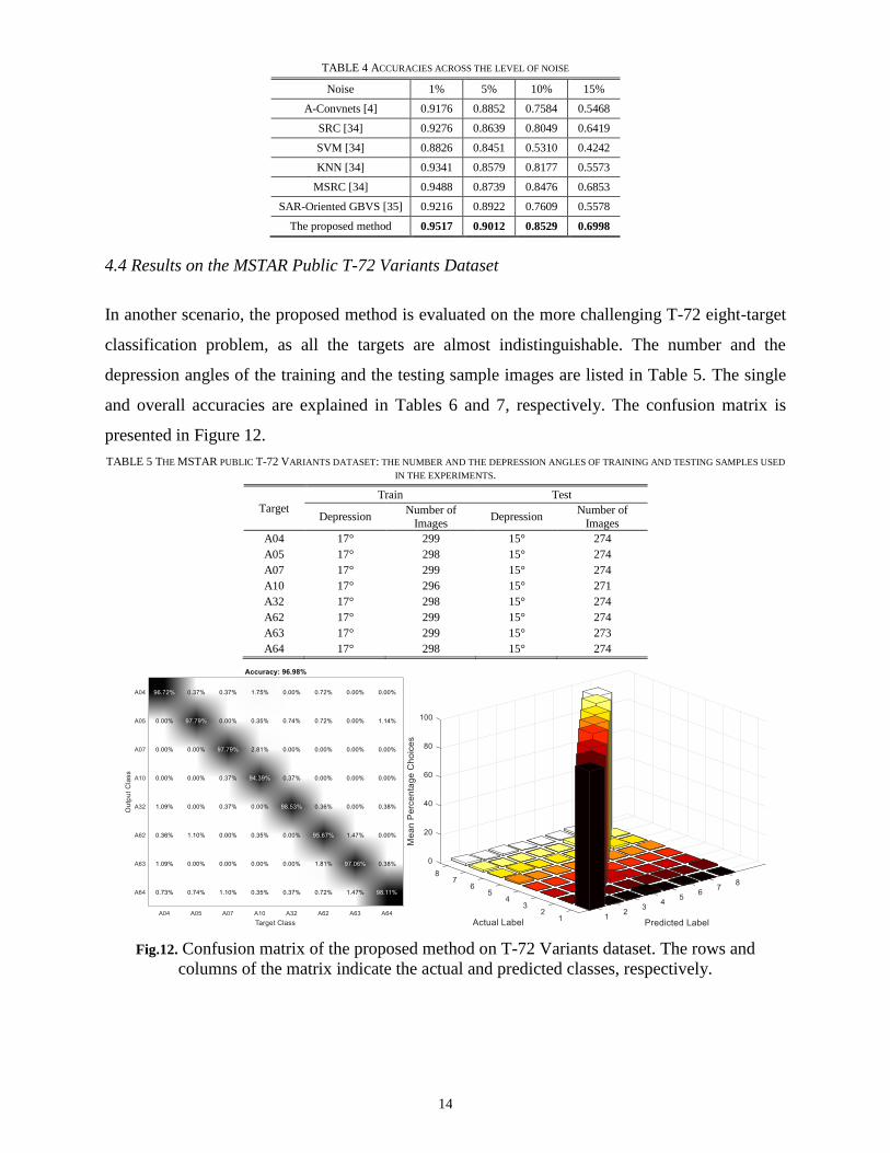
4.4 Results on the MSTAR Public T-72 Variants Dataset
In another scenario, the proposed method is evaluated on the more challenging T-72 eight-target
classification problem, as all the targets are almost indistinguishable. The number and the
depression angles of the training and the testing sample images are listed in Table 5. The single
and overall accuracies are explained in Tables 6 and 7, respectively. The confusion matrix is
presented in Figure 12.
TABLE 5 THE MSTAR PUBLIC T-72 VARIANTS DATASET: THE NUMBER AND THE DEPRESSION ANGLES OF TRAINING AND TESTING SAMPLES USED
IN THE EXPERIMENTS.
Target
Train Test
Depression Number of
Images Depression
Number of
Images
A04 17° 299 15° 274
A05 17° 298 15° 274
A07 17° 299 15° 274
A10 17° 296 15° 271
A32 17° 298 15° 274
A62 17° 299 15° 274
A63 17° 299 15° 273
A64 17° 298 15° 274
Fig.12. Confusion matrix of the proposed method on T-72 Variants dataset. The rows and
columns of the matrix indicate the actual and predicted classes, respectively.

15
4.5 Results on the MSTAR with Large Depression Angle Variations
Since SAR images are very sensitive to depression angle variation, the credibility of the proposed
method is further evaluated on large depression angles. In these experiments, four targets (2S1,
BRDM-2, T-72, and ZSU-234) with 30° depression angle are assessed. The types and the number
of the considered SAR images are shown in Table 8.
TABLE 8 THE MSTAR PUBLIC DATABASE WITH 30° DEPRESSION ANGLE: THE NUMBER OF TRAINING AND TESTING SAMPLES USED IN THE
EXPERIMENTS.
Target Type Depression Number of
Images
2S1 B01 30° 288
BRDM-2 E71 30° 287
T-72 A64 30° 288
ZSU-234 D08 30° 288
The single and overall accuracies are presented in Tables 9 and 10, respectively. The confusion
matrix is shown in Figure 13.
4.6 Comparison with Different Fusion Methods
In order to study the sensitivity of the feature level fusion on classification on the MSTAR
database, we compared the classification accuracy with different fusion strategies (CCA, MCCA),
SAR-Oriented GBVS [35] and without feature fusion. As shown in Table 11, our proposed method
using MCCA achieves the best performance.
TABLE 2 THE CLASSIFICATION ACCURACY FOR EACH TARGET CLASS ON MSTAR PUBLIC MIXED TARGET DATASET
Cla
ss
Sin
gle
Acc
ura
cy
Err
or
Sin
gle
To
tal
Acc
ura
cy
Err
or
To
tal
Sen
siti
vit
y
Sp
ecif
icit
y
Pre
cisi
on
Fal
se
Po
siti
ve
Rat
e BMP-2 0.99825 0.0017452 0.10223 0 0.99825 1 1 0
BTR-70 1 0 0.10223 0.00017873 1 0.9998 0.99825 0.00019908
T-72 0.98255 0.017452 0.10063 0.00089366 0.98255 0.999 0.9912 0.00099562
BTR-60 0.99778 0.0022173 0.080429 0 0.99778 1 1 0
2S1 1 0 0.10241 0 1 1 1 0
BRDM-2 1 0 0.10223 0 1 1 1 0
D7 1 0 0.10223 0 1 1 1 0
T-62 1 0 0.10241 0 1 1 1 0
ZIL-131 0.99824 0.0017575 0.10152 0.00017873 0.99824 0.9998 0.99824 0.00019897
ZSU-234 0.99295 0.0070547 0.10063 0.0017873 0.99295 0.9980
1 0.98255 0.0019889
TABLE 3 THE OVERALL CLASSIFICATION ACCURACY MSTAR PUBLIC MIXED TARGET DATASET
Accuracy Error Sensitivity Specificity Precision False Positive Rate
0.9970 0.0030 0.9970 0.9997 0.9970 3.3825e-04

16
TABLE 6 THE CLASSIFICATION ACCURACY FOR EACH TARGET CLASS ON MSTAR PUBLIC T-72 VARIANTS DATASET
Cla
ss
Sin
gle
Acc
ura
cy
Err
or
Sin
gle
To
tal
Acc
ura
cy
Err
or
To
tal
Sen
siti
vit
y
Sp
ecif
icit
y
Pre
cisi
on
Fal
se
Po
siti
ve
Rat
e
A04 0.96715 0.032847 0.12112 0.0041133 0.96715 0.9953 0.96715 0.0047022
A05 0.9708 0.029197 0.12157 0.0027422 0.9708 0.99687 0.97794 0.0031348
A07 0.9708 0.029197 0.12157 0.0027422 0.9708 0.99687 0.97794 0.0031348
A10 0.99262 0.0073801 0.12294 0.0073126 0.99262 0.99165 0.94386 0.0083464
A32 0.9781 0.021898 0.12249 0.0018282 0.9781 0.99791 0.98529 0.0020899
A62 0.96715 0.032847 0.12112 0.0054845 0.96715 0.99373 0.95668 0.0062696
A63 0.96703 0.032967 0.12066 0.0036563 0.96703 0.99582 0.97059 0.0041775
A64 0.94526 0.054745 0.11837 0.0022852 0.94526 0.99739 0.98106 0.0026123
TABLE 7 THE OVERALL CLASSIFICATION ACCURACY ON MSTAR PUBLIC T-72 VARIANTS DATASET
Accuracy Error Sensitivity Specificity Precision False Positive Rate
0.9698 0.0302 0.9699 0.9957 0.9701 0.0043
TABLE 9 THE CLASSIFICATION ACCURACY FOR EACH TARGET CLASS ON MSTAR PUBLIC DATABASE WITH 30° DEPRESSION ANGLE
Cla
ss
Sin
gle
Acc
ura
cy
Err
or
Sin
gle
Acc
ura
cy
in
To
tal
Err
or
in
To
tal
Sen
siti
vit
y
Sp
ecif
icit
y
Pre
cisi
on
Fal
se
Po
siti
ve
Rat
e
2S1 0.98958 0.010417 0.24761 0.0026064 0.98958 0.99652 0.98958 0.0034762
BRDM-2 0.98955 0.010453 0.24674 0.004344 0.98955 0.99421 0.9827 0.005787
T-72 0.98264 0.017361 0.24587 0.0026064 0.98264 0.99652 0.98951 0.0034762
ZSU-234 0.99306 0.0069444 0.24848 0.0017376 0.99306 0.99768 0.99306 0.0023175
TABLE 10 THE OVERALL CLASSIFICATION ACCURACY ON MSTAR PUBLIC DATABASE WITH 30° DEPRESSION ANGLE
Accuracy Error Sensitivity Specificity Precision False Positive Rate
0.9887 0.0113 0.9887 0.9962 0.9887 0.0038
TABLE 11 COMPARISON WITH DIFFERENT FUSION METHODS ON MSTAR DATABASE
Method MSTAR
public mixed
target (%)
MSTAR public T-72 Variants
(%)
MSTAR with
30° (%)
Proposed without fusion 98.79 94.50 96.13
VDCCA 99.12 95.31 97.55
VDMCCA 99.70 96.98 98.87
SAR-Oriented GBVS [35] 99.68 96.90 98.70

17
Fig.13. Confusion matrix of the proposed method on MSTAR with large depression angle
variations. The rows and columns of the matrix indicate the actual and predicted classes,
respectively.
4.7 Influence of Number of Layers and Different Receptive Fields on the Results
To study the effect of network depth on its accuracy in SAR image recognition setting, several
successful CNN models pre-trained on MSTAR are evaluated in our work, which are the famous
baseline model AlexNet, the Caffe reference model (CaffeRef), and the VGG network [36]. Due
to a large learning capacity, dominant expressive power and hierarchical structure of our SAR
oriented very deep network (19 layers): a high-level, semantic and robust feature representation
for each region proposal is obtained as it is illustrated in Table 12.
TABLE 12 THE EFFECT OF NETWORK DEPTH ON THE PERFORMANCE
Accuracy (%) MSTAR
public
mixed
MSTAR
T-72
Variants
MSTAR
depression
30° Models Conv1 Conv2 Conv3 Conv4 Conv5 Fc1 Fc2 Fc3
AlexNet 11×11×96 5×5×256 3×3×384 3×3×384 3×3×256 4096
dropout
4096
dropout
C
softmax 95.21 86.82 89.66
CaffeRef 11×11×96 5×5×256 3×3×384 3×3×384 3×3×256 4096
dropout 4096
dropout C
softmax 95.45 85.96 88.99
VGGF 11×11×64 5×5×256 3×3×256 3×3×256 3×3×256 4096
dropout
4096
dropout
C
softmax 95.66 86.9 90.6
VGGM 7×7×96 5×5×256 3×3×512 3×3×512 3×3×512 4096
dropout 4096
dropout C
softmax 96.7 88.08 91.5
VGGM-
128 7×7×96 5×5×256 3×3×512 3×3×512 3×3×512
4096
dropout
128
dropout
C
softmax 96.13 89.43 90.12
VGGM-1024
7×7×96 5×5×256 3×3×512 3×3×512 3×3×512 4096
dropout 1024
dropout C
softmax 97.6 90.86 91.6
VGGM-
2048 7×7×96 5×5×256 3×3×512 3×3×512 3×3×512
4096
dropout
2048
dropout
C
softmax 96.74 90.12 91.55
VGGS 7×7×96 5×5×256 3×3×512 3×3×512 3×3×512 4096
dropout 4096
dropout C
softmax 97.95 91.66 92.88
VGG16 16 weight layers including 13 convolutional layers 3×3 and 3 fully-connected layers 99.1 95.39 97.1
SAR-OVDN (19 weight layers including 16 convolutional layers and 3 fully-connected layers) 99.7 96.98 98.87

18
In addition, using a stack of two 3 × 3 convolutional layers (without pooling in between) has a 5
× 5 effective receptive field, and using three of 3 × 3 layers has a 7 × 7 effective receptive field.
So the reasons for using, for instance, a stack of three 3×3 convolutional layers instead of a single
7×7 layer are: First, we integrate three non-linear rectification layers rather than one, which leads
to a more discriminative decision function. Second, we reduce the number of parameters by
supposing that the three layer 3 × 3 convolution stack has K channels, and the stack is
parameterized by 3(32K2) = 27K2 weights; in contrast to a single 7 × 7 convolutional layer which
requires 72K2 = 49K2, which needs 81% more of parameters.
4.8 Comparison with Recent Representative Methods
The classification performance of the proposed method is compared with the most widely cited
approaches and the recent representative paradigms such as: MSRC [34], SVM [37], Cond Gauss
[38], MSS [39], A-Convnets [4], CNN [5], BCS [40], CNN–SVM [15] and Deep Leaning [16].
Because the SVM method [37] only considers the three-target classification problem, we have run
the published online code from [37] to obtain the results on our classification tasks (ten targets, T-
72 Variants, and 30° depression angle). All other compared methods do the same classification
tasks as ours. Therefore, we directly use the classification accuracies presented in the
corresponding papers. As illustrated in Table 12, our proposed method achieves the highest
accuracy rates. Fig. 14 shows MSTAR/IU Mixed Targets recognition results based on MF datasets.
Fig. 14. MSTAR/IU Mixed Targets recognition results using different MF datasets

19
TABLE 13
THE PERFORMANCE COMPARISON BETWEEN THE PROPOSED METHOD AND THE STATE-OF-THE-ART METHODS ON THE MSTAR PUBLIC DATABASE
Method
MSTAR
public mixed target (%)
MSTAR public
T-72 Variants (%)
MSTAR with
30° (%)
SVM [37] 90 78.5 81
Cond Gauss [38] 97 77.32 80
MSRC [34] 93.6 - 98.4
MSS [39] 96.6 - 98.2
CNN [5] 84.7 81.08 81.56
A-Convnets [4] 99.13 95.43 96.12
BCS [40] 92.6 88.76 92.6
Deep Leaning [16] 92.74 - -
CNN–SVM [15] 99.5 95.75 96.6
Proposed with softmax 99.51 96.13 98.34
Proposed with SVM 99.70 96.98 98.87
5 Conclusion
This paper developed SAR Oriented network to automatically learn very deep features from the
data sets, selects adaptive feature layers, and fuses the learned features. The proposed network
increases the depth by using more convolutional layers to lessen the speckle noise effect. A dropout
technique is supplied to deal with the over-fitting problem due to limited training data sets. In
addition, the MCCA algorithm is introduced to combine the selective adaptive layer’s features and
improves the representations with respect to the correlation objective measured on SAR target
images, making the proposed method feasible for SAR image processing. Experimental results on
the benchmark of MSTAR database demonstrate the effectiveness of the proposed method
compared with the state-of-the-art methods.
References
1. C. F. Olson and D. P. Huttenlocher, “Automatic target recognition by matching oriented edge
pixels,” IEEE Transactions on image processing, vol. 6, no. 1, pp. 103–113, 1997.
2. M. Amrani, S. Chaib, I. Omara, and F. Jiang, “Bag-of-visual-words based feature extraction for
sar target classification,” in Ninth International Conference on Digital Image Processing (ICDIP
2017), vol. 10420. International Society for Optics and Photonics, 2017, p. 104201J.
3. Amrani, M., Yang, K., Zhao, D., Fan, X., & Jiang, F. (2017, September). An efficient feature
selection for SAR target classification. In Pacific Rim Conference on Multimedia (pp. 68-78).
Springer, Cham.

20
4. S. Chen, H. Wang, F. Xu, and Y.-Q. Jin, “Target classification using the deep convolutional
networks for sar images,” IEEE Transactions on Geoscience and Remote Sensing, vol. 54, no. 8,
pp. 4806–4817, 2016.
5. N. Srivastava, G. E. Hinton, A. Krizhevsky, I. Sutskever, and R. Salakhutdinov, “Dropout: a
simple way to prevent neural networks from overfitting.” Journal of machine learning research,
vol. 15, no. 1, pp. 1929–1958, 2014.
6. H. Furukawa, “Deep learning for target classification from sar imagery: Data augmentation and
translation invariance,” arXiv preprint arXiv:1708.07920, 2017.
7. S. Chen and H. Wang, “Sar target recognition based on deep learning,” in Data Science and
Advanced Analytics (DSAA), 2014 International Conference on. IEEE, 2014, pp. 541–547
8. K. Du, Y. Deng, R. Wang, T. Zhao, and N. Li, “Sar atr based on displacement-and rotation-
insensitive cnn,” Remote Sensing Letters, vol. 7, no. 9, pp. 895–904, 2016.
9. M. Amrani and F. Jiang, “Deep feature extraction and combination for synthetic aperture radar
target classification,” Journal of Applied Remote Sensing, vol. 11, no. 4, p. 042616, 2017.
10. D. C. Ciresan, U. Meier, J. Masci, L. Maria Gambardella, and J. Schmidhuber, “Flexible, high
performance convolutional neural networks for image classification,” in IJCAI Proceedings-
International Joint Conference on Artificial Intelligence, vol. 22, no. 1. Barcelona, Spain, 2011,
p. 1237.
11. I. J. Goodfellow, Y. Bulatov, J. Ibarz, S. Arnoud, and V. Shet, “Multi-digit number recognition
from street view imagery using deep convolutional neural networks,” arXiv preprint
arXiv:1312.6082, 2013.
12. C. Szegedy, W. Liu, Y. Jia, P. Sermanet, S. Reed, D. Anguelov, D. Erhan, V. Vanhoucke, and
A. Rabinovich, “Going deeper with convolutions, corr abs/1409.4842,” URL http://arxiv.
org/abs/1409.4842, 2014.
13. K. Simonyan and A. Zisserman, “Very deep convolutional networks for large-scale image
recognition,” arXiv preprint arXiv:1409.1556, 2014.
14. C. P. Schwegmann, W. Kleynhans, B. P. Salmon, L. W. Mdakane, and R. G. Meyer, “Very deep
learning for ship discrimination in synthetic aperture radar imagery,” in Geoscience and Remote
Sensing Symposium (IGARSS), 2016 IEEE International. IEEE, 2016, pp. 104–107.
15. A. Bochkovskiy, C. Y. Wang, and H. Liao, “YOLOv4: Optimal speed and accuracy of object
detection,” arXiv preprint arXiv:2004.10934, 2020.
16. S. A. Wagner, “Sar atr by a combination of convolutional neural network and support vector
machines,” IEEE Transactions on Aerospace and Electronic Systems, vol. 52, no. 6, pp. 2861–
2872, 2016.
17. F. Zhou, L. Wang, X. Bai, and Y. Hui, "SAR ATR of ground vehicles based on LM-BN-CNN",
IEEE Transactions on Geoscience and Remote Sensing, 2018.
18. E. Mason, B. Yonel, and B. Yazici, “Deep learning for radar,” in Radar Conference
(RadarConf), 2017 IEEE. IEEE, 2017, pp. 1703–1708.
19. Y. LeCun, K. Kavukcuoglu, and C. Farabet, “Convolutional networks and applications in vision,”
in Circuits and Systems (ISCAS), Proceedings of 2010 IEEE International Symposium on. IEEE,
2010, pp. 253–256.
20. Y. Tang, “Deep learning using linear support vector machines,” arXiv preprint arXiv:1306.0239,
2013.

21
21. C. Liu and H. Wechsler, “A shape-and texture-based enhanced fisher classifier for face
recognition,” IEEE transactions on image processing, vol. 10, no. 4, pp. 598–608, 2001.
22. J. Yang and J.-y. Yang, “Generalized k–l transform based combined feature extraction,” Pattern
Recognition, vol. 35, no. 1, pp. 295–297, 2002.
23. C. Oliver and S. Quegan, Understanding synthetic aperture radar images. SciTech Publishing,
2004.
24. X. Huang, B. Zhang, H. Qiao, and X. Nie, “Local discriminant canonical correlation analysis for
supervised polsar image classification,” IEEE Geoscience and Remote Sensing Letters, vol. 14,
no. 11, pp. 2102–2106, 2017.
25. M. J. Canty, Image analysis, classification and change detection in remote sensing: with
algorithms for ENVI/IDL and Python. Crc Press, 2014.
26. G. Andrew, R. Arora, J. Bilmes, and K. Livescu, “Deep canonical correlation analysis,” in
International Conference on Machine Learning, 2013, pp. 1247–1255.
27. W. Krzanowski, Principles of multivariate analysis. OUP Oxford, 2000.
28. J. Ding, B. Chen, H. Liu, and M. Huang, “Convolutional neural network with data augmentation
for sar target recognition,” IEEE Geoscience and Remote Sensing Letters, vol. 13, no. 3, pp. 364–
368, 2016.
29. SDMS, “Mstar data,” https://www.sdms.afrl.af.mil/index.php? collection=mstar, last accessed:
2016-11-23.
30. El-Darymli, K., Mcguire, P., Gill, E. W., Power, D., & Moloney, C. (2015). Characterization and
statistical modeling of phase in single-channel synthetic aperture radar imagery. IEEE
Transactions on Aerospace and Electronic Systems, 51(3), 2071-2092.
31. Olivier, C., & Quegan, S. (1998). Understanding Synthetic Aperture Radar Images, Artech
House.
32. Vidal-Pantaleoni, A., & Marti, D. (2004). Comparison of different speckle-reduction techniques
in SAR images using wavelet transform. International Journal of Remote Sensing, 25(22), 4915-
4932.
33. Choi, H., Yu, S., & Jeong, J. (2019, June). Speckle Noise Removal Technique in SAR Images
using SRAD and Weighted Least Squares Filter. In 2019 IEEE 28th International Symposium on
Industrial Electronics (ISIE) (pp. 1441-1446). IEEE.
34. G. Dong, N. Wang, and G. Kuang, “Sparse representation of monogenic signal: With application
to target recognition in sar images,” IEEE Signal Processing Letters, vol. 21, no. 8, pp. 952–956,
2014.
35. Amrani, M., Jiang, F., Xu, Y., Liu, S., & Zhang, S. (2018). SAR-oriented visual saliency model
and directed acyclic graph support vector metric based target classification. IEEE Journal of
Selected Topics in Applied Earth Observations and Remote Sensing, 11(10), 3794-3810.
36. Zhou, W., Newsam, S., Li, C., & Shao, Z. (2017). Learning low dimensional convolutional neural
networks for high-resolution remote sensing image retrieval. Remote Sensing, 9(5), 489.
37. U. Srinivas, V. Monga, and R. G. Raj, “Sar automatic target recognition using discriminative
graphical models,” IEEE transactions on aerospace and electronic systems, vol. 50, no. 1, pp.
591–606, 2014
38. J. A. O’Sullivan, M. D. DeVore, V. Kedia, and M. I. Miller, “Sar atr performance using a
conditionally gaussian model,” IEEE Transactions on Aerospace and Electronic Systems, vol.
37, no. 1, pp. 91–108, 2001.

22
39. G. Dong and G. Kuang, “Classification on the monogenic scale space: application to target
recognition in sar image,” IEEE Transactions on Image Processing, vol. 24, no. 8, pp. 2527–
2539, 2015.
40. X. Zhang, J. Qin, and G. Li, “Sar target classification using bayesian compressive sensing with
scattering centers features,” Progress In Electromagnetics Research, vol. 136, pp. 385–407, 2013.