1 / 36

New proof that the sum of natural number is -1/12 of zeta function

K. Sugiyama1

Published 2014/03/30; revised 2015/02/15.

Abstract

We prove that the sum of natural number is -1/12 of the value of the zeta function by the new

method.

Abel calculated the sum of the divergent series by the Abel summation method. However, we

cannot calculate the sum of natural number by the method. In this paper, we calculate the sum of the

natural number by the extended Abel summation method.

2010 Mathematics Subject Classification: Primary 11M06; Secondary 11B65.

CONTENTS 1 Introduction .................................................................................................................................. 1

1.1 Issue ..................................................................................................................................... 1

1.2 Importance of the issue ........................................................................................................ 2

1.3 Research trends so far .......................................................................................................... 2

1.4 New derivation method of this paper ................................................................................... 2

1.5 Old method by Abel summation method ............................................................................. 2

2 New method ................................................................................................................................. 5

2.1 New method by new proposition ......................................................................................... 5

2.2 Proof of the proposition 1 .................................................................................................... 7

2.3 Proof of the proposition 2 .................................................................................................... 7

3 Conclusion ................................................................................................................................. 10

4 Future issues ............................................................................................................................... 10

5 Supplement................................................................................................................................. 10

5.1 Numerical calculation ........................................................................................................ 10

5.2 Singular equation ............................................................................................................... 11

5.3 General damped oscillation summation method ................................................................ 14

5.4 Definition of the propositions by the (ε, δ)-definition of limit .......................................... 20

5.5 Relation with q-analog ....................................................................................................... 23

5.5.1 q-analog ......................................................................................................................... 23

5.5.2 Zeta function .................................................................................................................. 24

5.5.3 Analytic zeta function .................................................................................................... 27

5.6 Reflection integral equation ............................................................................................... 30

6 Appendix .................................................................................................................................... 32

6.1 Hurwitz zeta function ......................................................................................................... 32

6.2 Lerch zeta function ............................................................................................................. 34

6.3 Goursat's theorem ............................................................................................................... 34

7 Bibliography............................................................................................................................... 35

1 Introduction

1.1 Issue

The integral representation of the zeta function converges by the analytic continuation. On the other

hand, the zeta function also has a series representation. One of the representation is the sum of all

2 / 36

natural numbers. The sum does not converge. It diverges. This paper converges the sum by the

extended Abel summation method.

"1 + 2 + 3 +⋯" = −1

12 (1.1)

1.2 Importance of the issue

It is desirable that both the integral representation and the series representation have a same value

for mathematical consistency. One method to converge the divergent series is Abel summation

method. The method converges the divergent series by multiplying convergence factor. However,

the sum of all natural numbers does not converge by the method. Therefore, it is an important issue

to find a new summation method.

1.3 Research trends so far

Leonhard Euler2 suggested that the sum of all natural numbers is −1/12 in 1749. Bernhard

Riemann3 showed that the integral representation of the zeta function is −1/12 in 1859. Srinivasa

Ramanujan4 proposed that the sum of all natural numbers is −1/12 by Ramanujan summation

method in 1913.

Niels Abel5 introduced Abel summation method in order to converge the divergent series in about

1829. J. Satoh6 constructed q-analogue of zeta-function in 1989. M. Kaneko, N. Kurokawa, and M.

Wakayama7 derived the sum of the double quoted natural numbers by the q-analogue of zeta-

function in 2002.

1.4 New derivation method of this paper

We define a new “sum of all natural numbers” by a new summation method, damped oscillation

summation method. The method converges the divergent series by multiplying convergence factor,

which is damped and oscillating very slowly. The traditional sum diverges for the infinite terms. On

the other hand, the new “sum” is equal to the traditional sum for the finite term. In addition, the

“sum” converges on −1/12 for the infinite term.

(Damped oscillation summation method for the sum of all natural numbers)

lim𝑥→0+

∑𝑘exp(−𝑘𝑥) cos(𝑘𝑥)

∞

𝑘=1

= −1

12 (1.2)

1.5 Old method by Abel summation method

Niels Abel introduced Abel summation method in about 1829.

We consider the following sum of the series.

𝑆 = ∑𝑎𝑘

∞

𝑘=1

(1.3)

3 / 36

Then we define the following function.

(Abel summation method)

𝐹(𝑥) = ∑𝑎𝑘 exp(−𝑘𝑥)

∞

𝑘=1

(1.4)

0 < 𝑥 (1.5)

We define Abel sum as follows.

𝑆𝐴 = lim𝑥→0+

𝐹(𝑥) (1.6)

We consider the following divergent series.

𝑆 = ∑(−1)𝑘−1𝑘

∞

𝑘=1

(1.7)

Then we define the following function.

𝐺(𝑥) = ∑(−1)𝑘−1𝑘 exp(−𝑘𝑥)

∞

𝑘=1

(1.8)

0 < 𝑥 (1.9)

Here, we will use the following formula.

(Formula of the geometric series that has coefficients of natural numbers)

∑𝑘𝑟𝑘∞

𝑘=1

=𝑟

(1 − 𝑟)2 (1.10)

We obtain the following equation by the above formula.

𝐹(𝑥) =−𝑒−𝑥

(1 + 𝑒−𝑥)2 (1.11)

We calculate the Abel sum as follows.

𝑆𝐴 = lim𝑥→0+

𝐹(𝑥) =−𝑒−0

(1 + 𝑒−0)2= −

1

4 (1.12)

Abel calculated the sum of the divergent series by the Abel summation method as above stated.

However, we cannot calculate the sum of natural number by the method.

We consider the following sum of all natural numbers.

4 / 36

𝑆 = ∑𝑘

∞

𝑘=1

(1.13)

Then we define the following function.

𝐺(𝑥) = ∑𝑘 exp(−𝑘𝑥)

∞

𝑘=1

(1.14)

0 < 𝑥 (1.15)

Here, we will use the following formula.

(Formula of the geometric series that has coefficients of natural numbers)

∑𝑘𝑟𝑘∞

𝑘=1

=𝑟

(1 − 𝑟)2 (1.16)

We obtain the following equation by the above formula.

𝐺(𝑥) =𝑒−𝑥

(1 − 𝑒−𝑥)2 (1.17)

We calculate the Abel sum as follows.

𝑆𝐴 = lim𝑥→0+

𝐺(𝑥) =−𝑒−0

(1 − 𝑒−0)2= ∞ (1.18)

The Abel sum diverges as above stated. Therefore, we cannot caluculate the sum of the natural

number by the method.

In order to examine the mechanism of the divergence, we use the following definitional formula of

Bernoulli numbers.

(Definitional formula of Bernoulli numbers)

𝑧𝑒𝑧

𝑒𝑧 − 1= ∑

𝐵𝑛𝑛!

𝑧𝑛∞

𝑛=0

(1.19)

In this paper, Bernoulli numbers Bn is Bernoulli polynomial Bn (1).

We will square the both sides of the above formula. In addition, we will divide the both sides by z2.

Then we obtain the following equation.

𝑒2𝑧

(1 − 𝑒𝑧)2=

1

𝑧2(∑

𝐵𝑛𝑛!

𝑧𝑛∞

𝑛=0

)

2

(1.20)

5 / 36

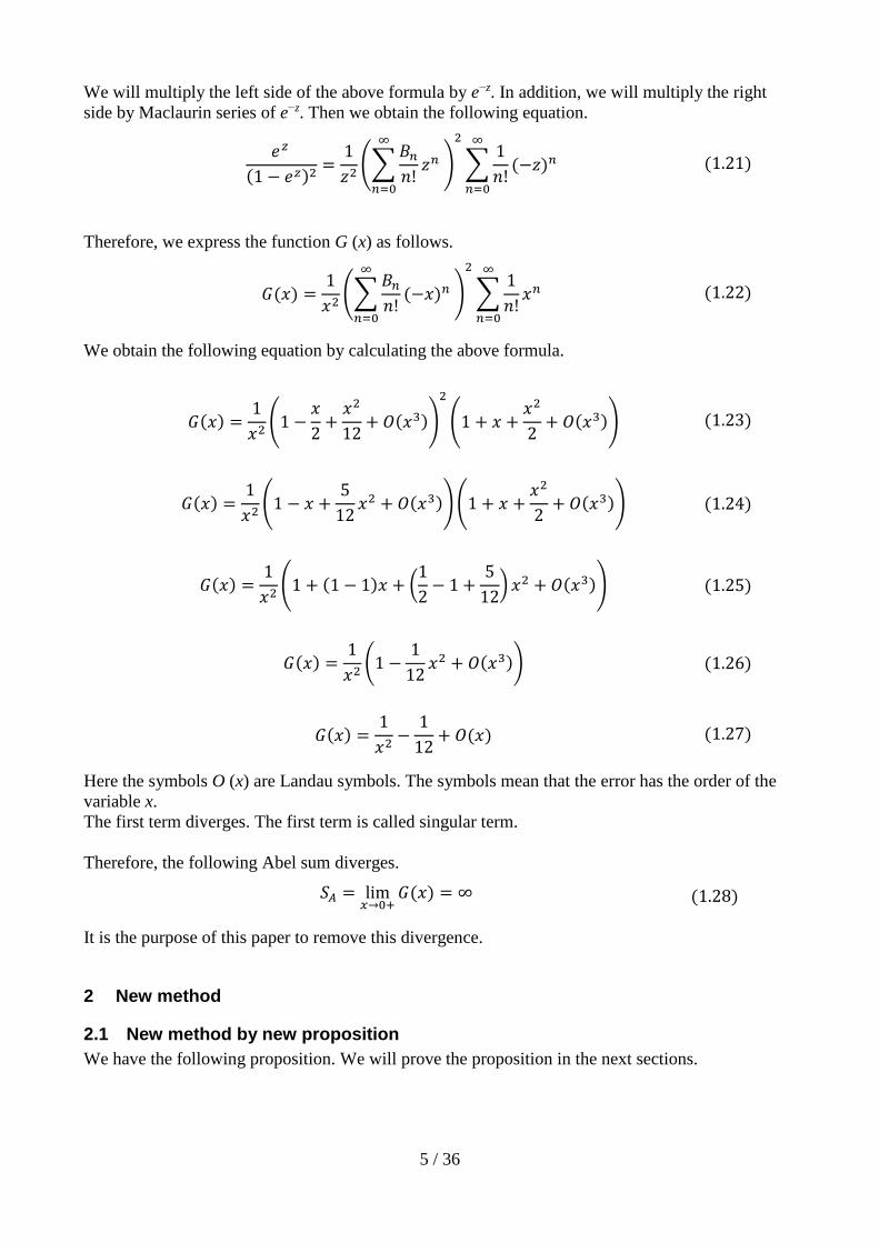
We will multiply the left side of the above formula by e−z. In addition, we will multiply the right

side by Maclaurin series of e−z. Then we obtain the following equation.

𝑒𝑧

(1 − 𝑒𝑧)2=

1

𝑧2(∑

𝐵𝑛𝑛!

𝑧𝑛∞

𝑛=0

)

2

∑1

𝑛!(−𝑧)𝑛

∞

𝑛=0

(1.21)

Therefore, we express the function G (x) as follows.

𝐺(𝑥) =1

𝑥2(∑

𝐵𝑛𝑛!

(−𝑥)𝑛∞

𝑛=0

)

2

∑1

𝑛!𝑥𝑛

∞

𝑛=0

(1.22)

We obtain the following equation by calculating the above formula.

𝐺(𝑥) =1

𝑥2(1 −

𝑥

2+𝑥2

12+ 𝑂(𝑥3))

2

(1 + 𝑥 +𝑥2

2+ 𝑂(𝑥3)) (1.23)

𝐺(𝑥) =1

𝑥2(1 − 𝑥 +

5

12𝑥2 + 𝑂(𝑥3))(1 + 𝑥 +

𝑥2

2+ 𝑂(𝑥3)) (1.24)

𝐺(𝑥) =1

𝑥2(1 + (1 − 1)𝑥 + (

1

2− 1 +

5

12) 𝑥2 + 𝑂(𝑥3)) (1.25)

𝐺(𝑥) =1

𝑥2(1 −

1

12𝑥2 + 𝑂(𝑥3)) (1.26)

𝐺(𝑥) =1

𝑥2−

1

12+ 𝑂(𝑥) (1.27)

Here the symbols O (x) are Landau symbols. The symbols mean that the error has the order of the

variable x.

The first term diverges. The first term is called singular term.

Therefore, the following Abel sum diverges.

𝑆𝐴 = lim𝑥→0+

𝐺(𝑥) = ∞ (1.28)

It is the purpose of this paper to remove this divergence.

2 New method

2.1 New method by new proposition

We have the following proposition. We will prove the proposition in the next sections.

6 / 36

Proposition 1.

lim𝑥→0+

∑𝑘exp(−𝑘𝑥) cos(𝑘𝑥)

𝑛

𝑘=1

= ∑𝑘

𝑛

𝑘=1

(2.1)

We have the following proposition. We will prove the proposition in the next sections, too.

Proposition 2.

lim𝑥→0+

∑𝑘exp(−𝑘𝑥) cos(𝑘𝑥)

∞

𝑘=1

= −1

12 (2.2)

We define the function Sn and Hn (x) as follows.

𝑆𝑛 = ∑𝑘

𝑛

𝑘=1

(2.3)

𝐻𝑛(𝑥) = ∑𝑘 exp(−𝑘𝑥) cos(𝑘𝑥)

𝑛

𝑘=1

(2.4)

Then we define the following symbols.

1 + 2 + 3 +⋯+ 𝑛 ∶= 𝑆𝑛 (2.5)

1 + 2 + 3 +⋯ ∶= lim𝑛→∞

𝑆𝑛 (2.6)

"1 + 2 + 3 +⋯+ 𝑛" ∶= lim𝑥→0+

𝐻𝑛(𝑥) (2.7)

"1 + 2 + 3 +⋯" ∶= lim𝑥→0+

( lim𝑛→∞

𝐻𝑛(𝑥)) (2.8)

Then we have the following propositions.

1 + 2 + 3 +⋯ = ∞ (2.9)

"1 + 2 + 3 +⋯+ 𝑛" = 1 + 2 + 3 +⋯+ 𝑛 (2.10)

"1 + 2 + 3 +⋯" = −1

12 (2.11)

The double quotes mean the analytic continuation of the sum of natural numbers.

7 / 36

The traditional sum diverges for the infinite terms. On the other hand, the new “sum” is equal to the

traditional sum for the finite term. In addition, the “sum” converges on −1/12 for the infinite term.

2.2 Proof of the proposition 1

Proposition 1.

lim𝑥→0+

∑𝑘exp(−𝑘𝑥) cos(𝑘𝑥)

𝑛

𝑘=1

= ∑𝑘

𝑛

𝑘=1

(2.12)

Proof. We define the function Hn (x) as follows.

𝐻𝑛(𝑥) = ∑𝑘 exp(−𝑘𝑥) cos(𝑘𝑥)

𝑛

𝑘=1

(2.13)

On the other hand, we have the following equation.

lim𝑥→0+

𝐻𝑛(𝑥) = ∑𝑘 exp(−𝑘0) cos(𝑘0)

𝑛

𝑘=1

= ∑𝑘

𝑛

𝑘=1

(2.14)

Therefore, we have the following equation.

lim𝑥→0+

∑𝑘exp(−𝑘𝑥) cos(𝑘𝑥)

𝑛

𝑘=1

= ∑𝑘

𝑛

𝑘=1

(2.15)

This completes the proof.

2.3 Proof of the proposition 2

Proposition 2.

lim𝑥→0+

∑𝑘exp(−𝑘𝑥) cos(𝑘𝑥)

∞

𝑘=1

= −1

12 (2.16)

Proof. We consider the following sum of all natural numbers.

𝑆 = ∑𝑘

∞

𝑘=1

(2.17)

Then we define the following function.

8 / 36

𝐻(𝑥) ∶= ∑𝑘 exp(−𝑘𝑥) cos(𝑘𝑥)

∞

𝑘=1

(2.18)

0 < 𝑥 (2.19)

Here, we use the following formula.

(Euler's formula)

exp(𝑖𝜃) = cos(𝜃) + 𝑖 sin(𝜃) (2.20)

We obtain the following formula from the above formula.

cos(𝜃) =1

2(exp(𝑖𝜃) + exp(−𝑖𝜃)) (2.21)

We obtain the following formula from the above formula by putting θ = k x.

cos(𝑘𝑥) =1

2(exp(𝑖𝑘𝑥) + exp(−𝑖𝑘𝑥)) (2.22)

Hence, we express the function H (x) as follows.

𝐻(𝑥) = ∑𝑘 exp(−𝑘𝑥)1

2(exp(𝑖𝑘𝑥) + exp(−𝑖𝑘𝑥))

∞

𝑘=1

(2.23)

𝐻(𝑥) =1

2∑𝑘 exp(−𝑘𝑥) exp(𝑖𝑘𝑥)

∞

𝑘=1

+1

2∑𝑘 exp(−𝑘𝑥) exp(−𝑖𝑘𝑥)

∞

𝑘=1

(2.24)

𝐻(𝑥) =1

2∑𝑘 exp(−𝑘𝑥 + 𝑖𝑘𝑥)

∞

𝑘=1

+1

2∑𝑘 exp(−𝑘𝑥 − 𝑖𝑘𝑥)

∞

𝑘=1

(2.25)

𝐻(𝑥) =1

2∑𝑘 exp(−𝑘(𝑥 − 𝑖𝑥))

∞

𝑘=1

+1

2∑𝑘 exp(−𝑘(𝑥 + 𝑖𝑥))

∞

𝑘=1

(2.26)

In addition, we define the following function.

𝐺(z) = ∑𝑘 exp(−𝑘𝑧)

∞

𝑘=1

(2.27)

𝑧 ∈ ℂ (2.28)

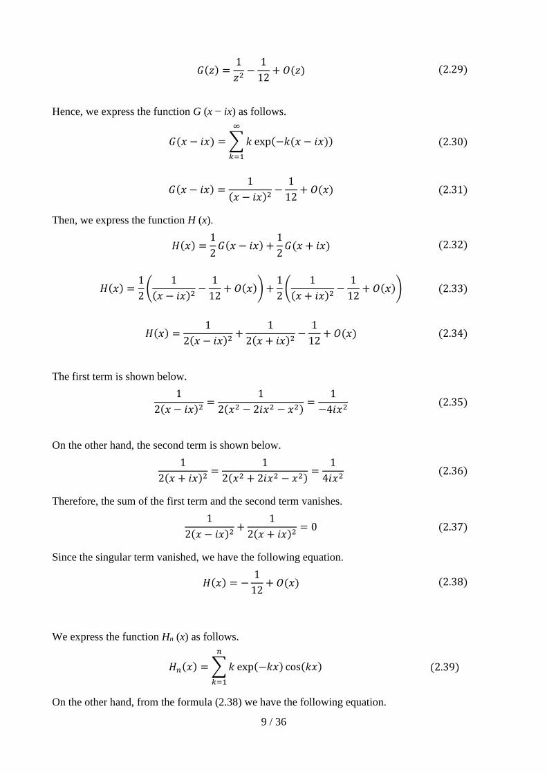
We express the function G (z) from the formula (1.27).

9 / 36

𝐺(𝑧) =1

𝑧2−

1

12+ 𝑂(𝑧) (2.29)

Hence, we express the function G (x − ix) as follows.

𝐺(𝑥 − 𝑖𝑥) = ∑𝑘 exp(−𝑘(𝑥 − 𝑖𝑥))

∞

𝑘=1

(2.30)

𝐺(𝑥 − 𝑖𝑥) =1

(𝑥 − 𝑖𝑥)2−

1

12+ 𝑂(𝑥) (2.31)

Then, we express the function H (x).

𝐻(𝑥) =1

2𝐺(𝑥 − 𝑖𝑥) +

1

2𝐺(𝑥 + 𝑖𝑥) (2.32)

𝐻(𝑥) =1

2(

1

(𝑥 − 𝑖𝑥)2−

1

12+ 𝑂(𝑥)) +

1

2(

1

(𝑥 + 𝑖𝑥)2−

1

12+ 𝑂(𝑥)) (2.33)

𝐻(𝑥) =1

2(𝑥 − 𝑖𝑥)2+

1

2(𝑥 + 𝑖𝑥)2−

1

12+ 𝑂(𝑥) (2.34)

The first term is shown below.

1

2(𝑥 − 𝑖𝑥)2=

1

2(𝑥2 − 2𝑖𝑥2 − 𝑥2)=

1

−4𝑖𝑥2 (2.35)

On the other hand, the second term is shown below.

1

2(𝑥 + 𝑖𝑥)2=

1

2(𝑥2 + 2𝑖𝑥2 − 𝑥2)=

1

4𝑖𝑥2 (2.36)

Therefore, the sum of the first term and the second term vanishes.

1

2(𝑥 − 𝑖𝑥)2+

1

2(𝑥 + 𝑖𝑥)2= 0 (2.37)

Since the singular term vanished, we have the following equation.

𝐻(𝑥) = −1

12+ 𝑂(𝑥) (2.38)

We express the function Hn (x) as follows.

𝐻𝑛(𝑥) = ∑𝑘 exp(−𝑘𝑥) cos(𝑘𝑥)

𝑛

𝑘=1

(2.39)

On the other hand, from the formula (2.38) we have the following equation.

10 / 36

lim𝑛→∞

𝐻𝑛(𝑥) = ∑𝑘 exp(−𝑘𝑥) cos(𝑘𝑥)

∞

𝑘=1

= 𝐻(𝑥) = −1

12+ 𝑂(𝑥) (2.40)

Therefore, we have the following equation.

lim𝑥→0+

( lim𝑛→∞

𝐻𝑛(𝑥)) = lim𝑥→0+

(−1

12+ 𝑂(𝑥)) = −

1

12 (2.41)

This completes the proof.

3 Conclusion

We obtained the following results in this paper.

• We proved that the sum of natural number is -1/12 of the value of the zeta function by the new

method.

4 Future issues

The future issues are shown below.

• To study the relation between the damped oscillation summation and the q-analog.

5 Supplement

5.1 Numerical calculation

We will calculate the following value numerically.

𝐻 = ∑ 𝑘 exp(−𝑘0.01) cos(𝑘0.01)

3000

𝑘=1

(5.1)

The result is shown below.

𝐻 = −0.0833333498⋯ (5.2)

This value is very close to the following −1/12.

−1

12= −0.0833333333⋯ (5.3)

The graph is shown in the Figure 5.1.

11 / 36

Figure 5.1: Damped oscillation of natural number

Here, we will double the attenuation factor as follows. We do not change the vibration period.

𝐻 = ∑ 𝑘 exp(−𝑘0.02) cos(𝑘0.01)

3000

𝑘=1

(5.4)

The result is shown below.

𝐻 = 1199.9166679⋯ (5.5)

Therefore, the series does not converge if the attenuation factor and the vibration period do not have

a special relation. We will consider the relation in the next section.

5.2 Singular equation

We consider the following series.

𝑆 = ∑𝑎𝑘

∞

𝑘=1

(5.6)

Then we define the following function.

-20

-15

-10

-5

0

5

10

15

20

25

30

1.0

12 / 36

𝐻(𝑥) = ∑𝑎𝑘 exp(−𝑘𝜙(𝑥)) cos(𝑘𝑥)

∞

𝑘=1

(5.7)

0 < 𝑥 (5.8)

0 < 𝜙(𝑥) (5.9)

In addition, we define the following function.

𝐺(z) = ∑𝑘 exp(−𝑘𝑧)

∞

𝑘=1

(5.10)

𝑧 ∈ ℂ (5.11)

We express the function G (z) by using singular term A (z), and the constant C.

𝐺(𝑧) = 𝐴(𝑧) + 𝐶 + 𝑂(𝑧) (5.12)

Here, we use the following formula.

(Euler's formula)

exp(𝑖𝜃) = cos(𝜃) + 𝑖 sin(𝜃) (5.13)

We express the function H (x) as follows by using the above formula.

𝐻(𝑥) =1

2(𝐺(𝑧) + 𝐺(𝑧̅)) (5.14)

𝑧 = 𝜙(𝑥) + 𝑖𝑥 (5.15)

𝑧̅ = 𝜙(𝑥) − 𝑖𝑥 (5.16)

We obtain the following equation by using the formula (5.12) of the function G (z).

𝐻(𝑥) =1

2(𝐴(𝑧) + 𝐴(z̅)) + 𝐶 + 𝑂(𝑧) (5.17)

We determine the function ϕ (x) by the following singular equation in order to remove the singular

term of the above equation.

(Singular equation)

1

2(𝐴(𝑧) + 𝐴(𝑧̅)) = 𝑂(𝑧) (5.18)

The series a k and the function G (z) and ϕ (x) are shown below.

13 / 36

Series 𝑎𝑘 Function 𝐺(𝑧) Function 𝜙(𝑥)

1 𝐺(𝑧) = −1

𝑧−1

2+ 𝑂(𝑧) 𝜙(𝑥) =

𝑥

tan(𝜋/2)+ 𝑂(𝑥3)

𝑘 𝐺(𝑧) =1

𝑧2−

1

12+ 𝑂(𝑧) 𝜙(𝑥) =

𝑥

tan(𝜋/4)+ 𝑂(𝑥4)

𝑘2 𝐺(𝑧) = −2

𝑧3+ 𝑂(𝑧) 𝜙(𝑥) =

𝑥

tan(𝜋/6)+ 𝑂(𝑥5)

𝑘3 𝐺(𝑧) =6

𝑧4+

1

120+ 𝑂(𝑧) 𝜙(𝑥) =

𝑥

tan(𝜋/8)+ 𝑂(𝑥6)

The series and the example of the damped oscillation summation method are shown below.

Series 𝑎𝑘 Example of the damped oscillation summation method

1 𝐻(𝑥) = ∑1exp(−𝑘𝑥3) cos(𝑘𝑥)

∞

𝑘=1

𝑘 𝐻(𝑥) = ∑𝑘 exp(−𝑘𝑥) cos(𝑘𝑥)

∞

𝑘=1

𝑘2 𝐻(𝑥) = ∑𝑘2 exp(−𝑘𝑥√3) cos(𝑘𝑥)

∞

𝑘=1

𝑘3 𝐻(𝑥) = ∑𝑘3 exp (−𝑘𝑥(1 + √2)) cos(𝑘𝑥)

∞

𝑘=1

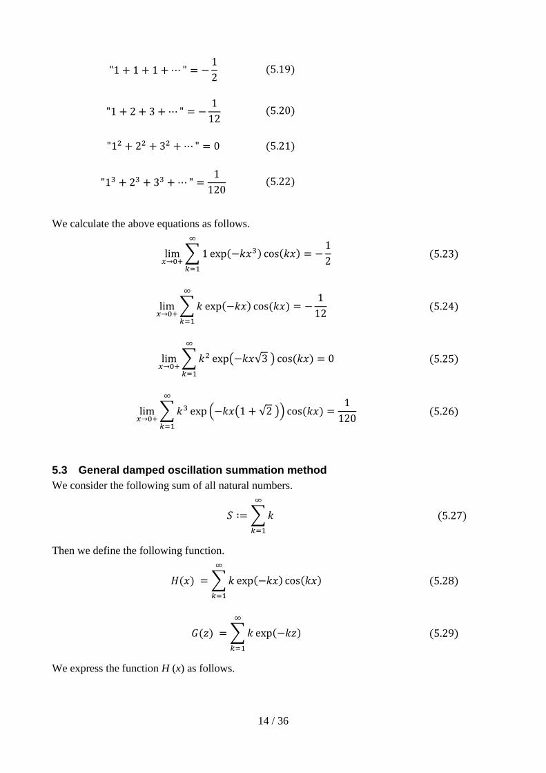
Therefore, we have the following equations.

14 / 36

"1 + 1 + 1 +⋯ " = −1

2 (5.19)

"1 + 2 + 3 +⋯" = −1

12 (5.20)

"12 + 22 + 32 +⋯" = 0 (5.21)

"13 + 23 + 33 +⋯" =1

120 (5.22)

We calculate the above equations as follows.

lim𝑥→0+

∑1exp(−𝑘𝑥3) cos(𝑘𝑥)

∞

𝑘=1

= −1

2 (5.23)

lim𝑥→0+

∑𝑘exp(−𝑘𝑥) cos(𝑘𝑥)

∞

𝑘=1

= −1

12 (5.24)

lim𝑥→0+

∑𝑘2 exp(−𝑘𝑥√3) cos(𝑘𝑥)

∞

𝑘=1

= 0 (5.25)

lim𝑥→0+

∑𝑘3 exp (−𝑘𝑥(1 + √2)) cos(𝑘𝑥)

∞

𝑘=1

=1

120 (5.26)

5.3 General damped oscillation summation method

We consider the following sum of all natural numbers.

𝑆 ∶= ∑𝑘

∞

𝑘=1

(5.27)

Then we define the following function.

𝐻(𝑥) = ∑𝑘 exp(−𝑘𝑥) cos(𝑘𝑥)

∞

𝑘=1

(5.28)

𝐺(𝑧) = ∑𝑘 exp(−𝑘𝑧)

∞

𝑘=1

(5.29)

We express the function H (x) as follows.

15 / 36

𝐻(𝑥) =1

2(𝐺(𝑥 − 𝑖𝑥) + 𝐺(𝑥 + 𝑖𝑥)) (5.30)

We interpret the above function as a sum of the function G (z1) and G (z2) like the following Figure

5.2.

Re(z)

Im(z)

O

G(z1)

G(z2)

Figure 5.2: Special damped oscillation summation method

In the above Figure 5.2, the two functions G (z1) and G (z2) approach to the origin O at the two

angles. This is special condition. Is it possible to make the condition more general?

Then we consider the case that the many functions G (z) approach to the origin from the all points

on the circle of the radius x like the following Figure 5.3

16 / 36

Re(z)

Im(z)

O

G(z)

G(z)

G(z)

G(z)

x

G(z)

G(z)

G(z)

G(z)

G(z)

G(z)

G(z)

G(z)

Figure 5.3: General damped oscillation summation method

We express the above consideration in the following equations.

𝐻(𝑥) =1

2(𝐺(𝑧1) + 𝐺(𝑧2)) (5.31)

𝐻(𝑥) =1

3(𝐺(𝑧1) + 𝐺(𝑧2) + 𝐺(𝑧3)) (5.32)

𝐻(𝑥) =1

4(𝐺(𝑧1) + 𝐺(𝑧2) + 𝐺(𝑧3) + 𝐺(𝑧4)) (5.33)

𝐻(𝑥) =1

𝑛(𝐺(𝑧1) + 𝐺(𝑧2) + 𝐺(𝑧3) + ⋯+ 𝐺(𝑧𝑛)) (5.34)

𝐻(𝑥) = ∑1

𝑛𝐺(𝑧𝑘)

𝑛

𝑘=1

(5.35)

The function H (x) is the mean value of the function G (z).

We suppose that the circumference of the circle of the radius x is L. We express the circumference L

of the circle as follows.

17 / 36

𝐿 = 2𝜋𝑥 (5.36)

On the other hand, we express the circumference L as follows.

𝐿 = 𝑛|𝑧𝑘+1 − 𝑧𝑘| (5.37)

Therefore, we have the following equation.

2𝜋𝑥 = 𝑛|𝑧𝑘+1 − 𝑧𝑘| (5.38)

Then, we express the normalized constant 1/n as follows.

1

𝑛=|𝑧𝑘+1 − 𝑧𝑘|

2𝜋|𝑧𝑘| (5.39)

|𝑧𝑘| = 𝑥 (5.40)

On the other hand, the direction of −i (zk+1 − zk) is same as the direction of zk as shown in the Figure

5.4

Re(z)

Im(z)

O x

zk

zk +1

zk +1 - zk

-i (zk +1 - zk) -i

Figure 5.4: General damped oscillation summation method

Therefore, we express 1/n as follows.

18 / 36

1

𝑛=|𝑧𝑘+1 − 𝑧𝑘|

2𝜋|𝑧𝑘|=−𝑖(𝑧𝑘+1 − 𝑧𝑘)

2𝜋𝑧𝑘=−𝑖𝛿𝑧𝑘2𝜋𝑧𝑘

(5.41)

𝛿𝑧𝑘 ∶= 𝑧𝑘+1 − 𝑧𝑘 (5.42)

Therefore, we express the function H (x) as follows.

𝐻(𝑥) = ∑−𝑖𝛿𝑧𝑘

2𝜋𝑧𝑘𝐺(𝑧𝑘)

𝑛

𝑘=1

(5.43)

We express the above sum as the following integration.

𝐻(𝑥) = ∮−𝑖𝑑𝑧

2𝜋𝑧𝐺(𝑧)

|𝑧|=𝑥

(5.44)

𝐻(𝑥) = ∮𝑑𝑧

2𝜋𝑖𝑧𝐺(𝑧)

|𝑧|=𝑥

(5.45)

The above result is equal to the residue theorem. We can interpret the residue theorem the mean

value theorem of contour integration.

We obtain the following result by the residue theorem.

𝐻(𝑥) = ∮𝑑𝑧

2𝜋𝑖𝑧|𝑧|=𝑥

(1

𝑧2−

1

12+ 𝑂(𝑧)) = −

1

12 (5.46)

Therefore, we obtain the following new general summation method.

(General damped oscillation summation method)

𝑆 = ∑𝑎𝑘

∞

𝑘=1

(5.47)

𝐺(𝑧) = ∑𝑎𝑘 exp(−𝑘𝑧)

∞

𝑘=1

(5.48)

𝐻(𝑥) = ∮𝑑𝑧

2𝜋𝑖𝑧𝐺(𝑧)

|𝑧|=𝑥

(5.49)

𝑆𝐻 = lim𝑥→0+

𝐻(𝑥) (5.50)

This summation method can sum any series by the residue theorem.

We call the damped oscillation summation method with the residue theorem “general damped

oscillation summation method.”

19 / 36

We call the damped oscillation summation method without the residue theorem “special damped

oscillation summation method.”

20 / 36

5.4 Definition of the propositions by the (ε, δ)-definition of limit

The value of the limit depends on the order of the limit as follows.

lim𝑥→0

( lim𝑛→∞

∑𝑘𝑒−𝑘𝑥 cos(𝑘𝑥)

𝑛

𝑘=1

) = −1

12 (5.51)

lim𝑛→∞

(lim𝑥→0

∑𝑘𝑒−𝑘𝑥 cos(𝑘𝑥)

𝑛

𝑘=1

) = ∞ (5.52)

In this paper, we define the order of the limit as follows.

lim𝑥→0

∑𝑓𝑘(𝑥)

∞

𝑘=1

: = lim𝑥→0

( lim𝑛→∞

∑𝑓𝑘(𝑥)

𝑛

𝑘=1

) (5.53)

𝑓𝑘(𝑥) = 𝑘𝑒−𝑘𝑥 cos(𝑘𝑥) (5.54)

This order of the limit means the following relation.

0 ≪1

𝑥≪ 𝑛 (5.55)

We confirm the above relation by the (ε, δ)-definition of limit.

In this section, we define the following proposition by the (ε, δ)-definition of limit.

We define the function Sn and Hn (x), and the constant α as follows.

𝑆𝑛 = ∑𝑘

𝑛

𝑘=1

(5.56)

𝐻𝑛(𝑥) = ∑𝑘 exp(−𝑘𝑥) cos(𝑘𝑥)

𝑛

𝑘=1

(5.57)

𝛼 = −1

12 (5.58)

We have the following proposition.

lim𝑛→∞

𝑆𝑛 = ∞ (5.59)

We can express the above proposition by (R, N)-definition of the limit as follows.

Given any number R > 0, there exists a natural number N such that for all n satisfying

21 / 36

𝑁 < 𝑛, (5.60)

we have the following inequation.

𝑅 < 𝑆𝑛 (5.61)

We have the following proposition.

Proposition 1.

lim𝑥→0+

𝐻𝑛(𝑥) = 𝑆𝑛 (5.62)

We can express the above proposition by (ε, δ)-definition of the limit as follows.

Given any number x > 0 and any natural number n, there exists a number δ > 0 such that for all x >

0 satisfying

𝑥 < 𝛿, (5.63)

we have the following inequation.

|𝐻𝑛(𝑥) − 𝑆𝑛| < 휀 (5.64)

We can summarize the above definition as follows.

∀휀 > 0, ∀𝑛 ∈ ℕ, ∃𝛿 > 0s. t. ∀𝑥 > 0, 𝑥 < 𝛿 ⇒ |𝐻𝑛(𝑥) − 𝑆𝑛| < 휀

(5.65)

We have the following proposition.

Proposition 2.

lim𝑥→0+

( lim𝑛→∞

𝐻𝑛(𝑥)) = 𝛼 (5.66)

0 ≪1

𝑥≪ 𝑛 (5.67)

We can express the above proposition by (ε, δ)-definition of the limit as follows.

Given any number ε > 0, there exist a natural number N and a number δ > 0 such that for all n

satisfying

𝑁 < 𝑛, (5.68)

we have the following inequation.

|𝐻𝑛(𝛿) − 𝛼| < 휀 (5.69)

We can summarize the above definition as follows.

22 / 36

∀휀 > 0, ∃𝑁 ∈ ℕ, ∃𝛿 > 0s. t. ∀𝑛 ∈ ℕ,𝑁 < 𝑛 ⇒ |𝐻𝑛(𝛿) − 𝛼| < 휀

(5.70)

The proposition 1 is the region of 1+2+3+…+n and the proposition 2 is the region −1/12 in the

following figure.

1/x

O n N

1/δ

−1/12

1+2+3+…+n ε=0.01

Figure 5.5: (ε, δ)-definition of limit

23 / 36

5.5 Relation with q-analog

5.5.1 q-analog

F. H. Jackson8 defined the following quantized new natural number, q-number in 1904.

(q-number)

[𝑛]𝑞 ∶= 1 + 𝑞 + 𝑞2 +⋯+ 𝑞𝑛−1 (5.71)

[𝑛]𝑞 = ∑𝑞𝑘−1𝑛

𝑘=1

(5.72)

[𝑛]𝑞 =1 − 𝑞𝑛

1 − 𝑞 (5.73)

We call the quantized mathematical object q-analog generally. The q-analog of the natural number

n is q-number [n]q. We express the natural number by the classical limit of the q-number.

𝑛 = lim𝑞→1−

[𝑛]𝑞 (5.74)

The zeta function is shown below.

(Zeta function)

휁(𝑠) = ∑1

𝑛𝑠

∞

𝑛=1

(5.75)

The q-analog of the zeta function is q-zeta function. The function is shown below.7

(q-zeta function)

휁𝑞(𝑠) ∶= ∑1

[𝑛]𝑞𝑠 𝑞

𝑛(𝑠−1)

∞

𝑛=1

(5.76)

We express the zeta function by the classical limit of the q-zeta function.

휁(𝑠) = lim𝑞→1−

휁𝑞(𝑠) (5.77)

휁(𝑠) = ∑1

[𝑛]1𝑠 1

𝑛(𝑠−1)

∞

𝑛=1

(5.78)

휁(𝑠) = ∑1

𝑛𝑠

∞

𝑛=1

(5.79)

1 < Re(𝑠) (5.80)

24 / 36

5.5.2 Zeta function

This paper defines the following waved (quantized) new natural number, natural function.

(Natural function)

`n`𝑧 ∶= 𝑒𝑧 + 𝑒2𝑧 + 𝑒3𝑧 +⋯+ 𝑒𝑛𝑧 (5.81)

`𝑛`𝑧 = ∑𝑒𝑘𝑧𝑛

𝑘=1

(5.82)

`𝑛`𝑧 = 𝑒𝑧1 − 𝑒𝑛𝑧

1 − 𝑒𝑧 (5.83)

𝜈𝑛𝑧: = `𝜈𝑛`𝑧: = `𝑛`𝑧 (5.84)

The relation between the natural function and q-number as follows.

𝜈𝑛𝑧 = 𝑞[𝑛]𝑞 (5.85)

𝑞 = 𝑒𝑧 (5.86)

We differentiate the natural function by the variable z.

𝜈𝑛𝑧 = ∑𝑒𝑘𝑧𝑛

𝑘=1

(5.87)

𝑑

𝑑𝑧𝜈𝑛𝑧 = ∑𝑘𝑒𝑘𝑧

𝑛

𝑘=1

(5.88)

𝑑2

𝑑𝑧2𝜈𝑛𝑧 = ∑𝑘2𝑒𝑘𝑧

𝑛

𝑘=1

(5.89)

𝑑3

𝑑𝑧3𝜈𝑛𝑧 = ∑𝑘3𝑒𝑘𝑧

𝑛

𝑘=1

(5.90)

Therefore, we obtain the following function by differentiating the natural function by the variable z

m times.

𝑑𝑚

𝑑𝑧𝑚𝜈𝑛𝑧 = ∑𝑘𝑚𝑒𝑘𝑧

𝑛

𝑘=1

(5.91)

25 / 36

We define the following function, natural derivative by replacing the natural number m by the

complex s-1.

(Natural derivative)

`𝜈𝑛`𝑧(𝑠):= ∑𝑘𝑠−1𝑒𝑘𝑧𝑛

𝑘=1

(5.92)

𝜈𝑛𝑧(𝑠):= `𝜈𝑛`𝑧(𝑠) (5.93)

On the other hand, we define the natural number as follows.

(Natural number)

`𝑛` ∶= 1 + 1 + 1 +⋯+ 1 (5.94)

`𝑛` = ∑1

𝑛

𝑘=1

(5.95)

𝑛 = `𝑛` (5.96)

We express the natural number by a limit of the natural derivative.

𝑛 = lim𝑠→1

(lim𝑧→0

𝜈𝑛𝑧(𝑠)) (5.97)

𝑛 = ∑1

𝑘0𝑒𝑘0

𝑛

𝑘=1

(5.98)

𝑛 = ∑1

𝑛

𝑘=1

(5.99)

We define the zeta function as follows.

(Zeta function)

`휁`(𝑠) ∶=1

1s+

1

2s+

1

3s+⋯ (5.100)

`휁`(𝑠) = ∑1

𝑘𝑠

∞

𝑘=1

(5.101)

휁(𝑠): = `휁`(𝑠) (5.102)

We express the zeta function by a limit of the natural derivative.

26 / 36

휁(𝑠) = lim𝑧→0

(lim𝑛→0

𝜈𝑛𝑧(1 − 𝑠)) (5.103)

휁(𝑠) = ∑1

𝑘𝑠𝑒𝑘0

∞

𝑘=1

(5.104)

휁(𝑠) = ∑1

𝑘𝑠

∞

𝑘=1

(5.105)

We define the partition function as follows.

(Partition function)

`𝑍`(𝑧):= 𝑒𝑧 + 𝑒2𝑧 + 𝑒3𝑧 +⋯ (5.106)

`𝑍`(𝑧) = ∑𝑒𝑘𝑧∞

𝑘=1

(5.107)

𝑍(𝑧):= `𝑍`(𝑧) (5.108)

We express the partition function by a limit of the natural derivative.

𝑍(𝑧) = lim𝑠→1

( lim𝑛→∞

𝜈𝑛𝑧(𝑠)) (5.109)

𝑍(𝑧) = ∑𝑘1−1𝑒𝑘𝑧∞

𝑘=1

(5.110)

𝑍(𝑧) = ∑𝑒𝑘𝑧∞

𝑘=1

(5.111)

27 / 36

We summarize the above results as follows.

• The natural number is a limit of the natural derivative.

• The zeta function is a limit of the natural derivative.

• The partition function is a limit of the natural derivative.

We express these relations in the following figure.

Zeta function

)(s

Natural derivative

)(snz

Limit

Natural number

n

Partition function

)(zZ

Limit

Limit

Figure 5.6: Zeta function

5.5.3 Analytic zeta function

We define the harmonic natural derivative as follows by averaging (uncertainizing) the natural

derivative.

(Harmonic natural derivative)

"𝑛"𝜀(𝑠) ∶= ∮𝑑𝑧

2𝜋𝑖𝑧𝜈𝑛𝑧(𝑠)

|𝑧|=𝜀

(5.112)

𝜈𝑛𝜀(𝑠):= "𝜈𝑛"𝜀(𝑠):= "𝑛"𝜀(𝑠) (5.113)

We define the analytic zeta function as follows.

(Analytic zeta function)

28 / 36

"휁"(𝑠) ∶=1

Γ(𝑠)∫

𝑥𝑠−1

𝑒𝑥 − 1

∞

0

𝑑𝑥 (5.114)

휁(𝑠) ∶= "휁"(𝑠) (5.115)

The analytic zeta function is the analytic continuation of the zeta function.

We express the analytic zeta function by a limit of the harmonic natural derivative.

휁(𝑠) = lim𝑧→0

( lim𝑛→∞

𝜈𝑛𝜀(1 − 𝑠)) (5.116)

휁(𝑠) = lim𝑥→0

∮𝑑𝑧

2𝜋𝑖𝑧𝜈∞𝜀(1 − 𝑠)

|𝑧|=𝜀

(5.117)

휁(𝑠) = lim𝜀→0

∮𝑑𝑧

2𝜋𝑖𝑧∑

1

𝑘𝑠𝑒𝑘𝑧

∞

𝑘=1|𝑧|=𝜀

(5.118)

휁(𝑠) = lim𝜀→0

∮𝑑𝑧

2𝜋𝑖𝑧Li𝑠(𝑒

𝑧)|𝑧|=𝜀

(5.119)

Here, the function Lis (w) is the following polylogarithm function.

(Polylogarithm function)

Li𝑠(𝑤) = ∑1

𝑘𝑠𝑤𝑘

∞

𝑘=1

(5.120)

We obtain the following equation by using Taylor expansion of the Lis (ez).

Li𝑠(𝑒𝑧) = 𝑂 (

1

𝑧1−𝑠) + 휁(𝑠) + 휁(𝑠 − 1)𝑧 + 𝑂(𝑧2) (5.121)

The constant term of the Taylor expansion is the analytic zeta function. Therefore, we have the

following equation by using the residue theorem.

휁(𝑠) = limε→0

∮𝑑𝑧

2𝜋𝑖𝑧휁(𝑠)

|𝑧|=ε

(5.122)

We express these relations in the following figure.

29 / 36

1)(

z

z

e

ezH

)1(

)()(

s

ssh

)()()( sssg

)]([)( shZzH

)]([)( zGMsg )]([)( 1 zHZsh

)]([)( 1 sgMzG

)()( zGzH

)()( zHzG

1)(

z

z

e

ezG

Analytic

zeta function

)(s

Zeta function

)(s

Natural derivative

)(snz

Harmonic natural

derivative

)(sn

Analytic continuation

Limit

Average

Limit

Figure 5.7: Analytic zeta function

30 / 36

5.6 Reflection integral equation

We shoe the reflection integral equation of the natural derivative.

We define the factorial function by the gamma function as follows.

(Factorial function)

Π(𝑠) = Γ(𝑠)𝑠 (5.123)

We have the following equation for the natural number n.

Π(𝑛) = 𝑛! (5.124)

We define the falling factorial as follows.

(Falling factorial)

𝑠t =Π(𝑠)

Π(𝑠 − 𝑡) (5.125)

We have the following equation for the natural number n.

𝑛1 = (𝑛 − 0) (5.126)

𝑛2 = (𝑛 − 0)(𝑛 − 1) (5.127)

𝑛3 = (𝑛 − 0)(𝑛 − 1)(𝑛 − 2) (5.128)

We define the combination function by the beta function as follows.

(Combination function)

C(𝑠, 𝑡) =1

𝐵(𝑠, 𝑡)

𝑠 + 𝑡

𝑠𝑡 (5.129)

We have the following equation for the complex s, t.

C(𝑠, 𝑡) =Π(𝑠 + 𝑡)

Π(𝑠)Π(𝑡) (5.130)

We have the following equation for the natural number m, n.

C(𝑚, 𝑛) =(𝑚 + 𝑛)!

𝑚! 𝑛!= (

𝑚 + 𝑛𝑛

) (5.131)

We show the reflection integral equation of the complex as follows. 9

(Reflection integral equation of the complex)

𝜈𝑛𝑧(𝑠 + 1) = ∮𝑖𝑑𝑡

2𝜋B(𝑠, 𝑡)𝜈𝑛𝑧(−𝑡)

𝑆1 (5.132)

We express the equation by using the combination function as follows.

31 / 36

𝜈𝑛𝑧(𝑠 + 1) = ∮𝑖𝑑𝑡

2𝜋

1

C(𝑠, 𝑡)

𝑠 + 𝑡

𝑠𝑡𝜈𝑛𝑧(−𝑡)

𝑆1 (5.133)

We deform the equation as follows.

𝜈𝑛𝑧(𝑠 + 1) = ∮𝑖𝑑𝑡

2𝜋

𝜈𝑛𝑧(−𝑡)

C(𝑠 + 1, 𝑡)𝑡𝑆1 (5.134)

We replace the variable s+1 to s.

𝜈𝑛𝑧(𝑠) = ∮𝑖𝑑𝑡

2𝜋

𝜈𝑛𝑧(−𝑡)

C(𝑠, 𝑡)𝑡𝑆1 (5.135)

We show the reflection integral equation of the quaternion as follows. 10

(Reflection integral equation of the quaternion)

𝜈𝑛𝑧(𝑠 + 1) = ∮𝑑𝑡3

2𝜋2B(𝑠, 𝑡 + 2)

(𝑡 + 1)𝑡𝜈𝑛𝑧(−𝑡)

𝑆3 (5.136)

We express the equation by using the combination function as follows.

𝜈𝑛𝑧(𝑠 + 1) = ∮𝑑𝑡3

2𝜋21

C(𝑠, 𝑡 + 2)

𝑠 + 𝑡 + 2

𝑠(𝑡 + 2)

𝜈𝑛𝑧(−𝑡)

(𝑡 + 1)𝑡

𝑆3 (5.137)

We deform the equation as follows.

𝜈𝑛𝑧(𝑠 + 1) = ∮𝑑𝑡3

2𝜋2𝜈𝑛𝑧(−𝑡)

C(𝑠 + 1, 𝑡 + 2)(𝑡 + 2)3𝑆3 (5.138)

We replace the variable t to t-2.

𝜈𝑛𝑧(𝑠 + 1) = ∮𝑑𝑡3

2𝜋2𝜈𝑛𝑧(2 − 𝑡)

C(𝑠 + 1, 𝑡)𝑡3𝑆3 (5.139)

We replace the variable s+1 to s.

𝜈𝑛𝑧(𝑠) = ∮𝑑𝑡3

2𝜋2𝜈𝑛𝑧(2 − 𝑡)

C(𝑠, 𝑡)𝑡3𝑆3 (5.140)

We have the reflection integral equation of the complex and the quaternion as follows.

(Reflection integral equations)

𝜈𝑛𝑧(𝑠) = ∮𝑖𝑑𝑡

2𝜋𝑡

𝜈𝑛𝑧(−𝑡)

C(𝑠, 𝑡)𝑆1 (5.141)

𝜈𝑛𝑧(𝑠) = ∮𝑑𝑡3

2𝜋2𝑡3𝜈𝑛𝑧(2 − 𝑡)

C(𝑠, 𝑡)𝑆3 (5.142)

32 / 36

6 Appendix

6.1 Hurwitz zeta function

We calculate the sum of natural numbers by the Hurwitz zeta function.

Adolf Hurwitz11 published the following zeta function in 1882.

(Definitional series of Hurwitz zeta function)

휁(𝑠, 𝑞) =1

(𝑞 + 0)𝑠+

1

(𝑞 + 1)𝑠+

1

(𝑞 + 2)𝑠+⋯ (6.1)

휁(𝑠, 𝑞) = ∑

1

(𝑞 + 𝑘)𝑠

∞

𝑘=0

(6.2)

Hurwitz zeta function and Riemann zeta function have the following relationship.

(Relation between Hurwitz zeta function and Riemann zeta function)

휁(𝑠) = {1

1𝑠+

1

2𝑠+⋯+

1

(𝑞 − 1)𝑠} + {

1

(𝑞 + 0)𝑠+

1

(𝑞 + 1)𝑠+⋯} (6.3)

휁(𝑠) = ∑1

𝑘𝑠

𝑞−1

𝑘=1

+ 휁(𝑠, 𝑞) (6.4)

Therefore, we can observe the value of the sum to the middle of the sum of the natural numbers.

We calculate the Hurwitz zeta function by the following asymptotic expansion. Here, Bk is the

Bernoulli numbers.

(Asymptotic expansion of the Hurwitz zeta function)

휁(𝑠, 𝑞) = ∑𝐵𝑘𝑘!

𝑟

𝑘=0

Γ(𝑠 + 𝑘 − 1)

Γ(𝑠)𝑞𝑠+𝑘−1 (6.5)

For example, we think the sum of one until three and the sum of four until infinity.

휁(−1) = ∑1

𝑘−1

4−1

𝑘=1

+ 휁(−1,4) (6.6)

We can express the value of the Hurwitz zeta function as follows.

휁(−1,4) = ∑𝐵𝑘𝑘!

𝑟

𝑘=0

Γ(𝑘 − 2)

Γ(−1)4𝑘−2 (6.7)

Here, we use the following reflection formula of the gamma function.

33 / 36

Γ(1 − 𝑠) =𝜋

sin(𝜋𝑠)

1

Γ(𝑠) (6.8)

We can modified the Hurwitz zeta function as follows by the above formula.

휁(−1,4) = ∑𝐵𝑘𝑘!

𝑟

𝑘=0

Γ(2)

Γ(3 − 𝑘)4𝑘−2sin(2𝜋)

sin((3 − 𝑘)𝜋) (6.9)

We have the following equation for integer k.

sin(2𝜋)

sin((3 − 𝑘)𝜋)= (−1)𝑘+1 (6.10)

Therefore, we can obtain the following equation.

휁(−1,4) = ∑𝐵𝑘𝑘!

𝑟

𝑘=0

Γ(2)

Γ(3 − 𝑘)4𝑘−2(−1)𝑘+1 (6.11)

We have the following equation for integer k ≥ 3.

1

Γ(3 − 𝑘)= 0 (6.12)

Therefore, we can obtain the following equation.

휁(−1,4) =

𝐵01! (−1)0+1

0! (2 − 0)! 40−2+

𝐵11! (−1)1+1

1! (2 − 1)! 41−2+

𝐵21! (−1)2+1

2! (2 − 2)! 42−2 (6.13)

휁(−1,4) = (−

1

242) + (

1

241) + (−

1

1240) (6.14)

휁(−1,4) = −

16

2+4

2−

1

12 (6.15)

휁(−1,4) = −6 −

1

12 (6.16)

Therefore, we can obtain the following result.

"(1 + 2 + 3) + (4 + 5 + 6 +⋯)" = 6 + (−6 −1

12) = −

1

12 (6.17)

We can see that the sum of the natural numbers is increasing certainly halfway according the above

equation. Then, on the way leading to the infinity, it reduced.

The series of the zeta function seems to correct for negative integers.

However, why will it decrease on the way leading to the infinity?

34 / 36

I think that it oscillates in an infinite time on the way to infinity.

I think that it is damped exponentially on the way to infinity.

This idea became the origin of the damped oscillation summation method.

6.2 Lerch zeta function

This paper proposed that we might interpret Riemann zeta function as the Lerch zeta function in the

case of the variable λ is approximately zero.

The Lerch zeta function was published by Lerch12 in 1887.

(Definitional series of Lerch zeta function)

𝐿(𝜆, 𝛼, 𝑠) =exp(2𝜋𝑖𝜆0)

(0 + 𝛼)𝑠+exp(2𝜋𝑖𝜆1)

(1 + 𝛼)𝑠+exp(2𝜋𝑖𝜆2)

(2 + 𝛼)𝑠+⋯ (6.18)

𝐿(𝜆, 𝛼, 𝑠) = ∑exp(2𝜋𝑖𝜆𝑘)

(𝑘 + 𝛼)𝑠

∞

𝑘=0

(6.19)

6.3 Goursat's theorem

We derive the following theorem from the Cauchy's integral formula.

(Goursat's theorem of complex)

𝑓(𝑚)(𝑎) =𝑚!

2𝜋𝑖∫

𝑓(𝑧)

(𝑧 − 𝑎)𝑚+1𝐶

𝑑𝑧 (6.20)

Here, we consider the following partition function.

(Partition function)

𝑍(𝑧) = ∑𝑒𝑘𝑧∞

𝑘=1

=𝑒𝑧

1 − 𝑒𝑧 (6.21)

We express the above formla by Goursat's theorem.

𝑍(𝑚)(0) =𝑚!

2𝜋𝑖∫

𝑍(𝑧)

𝑧𝑚+1𝐶

𝑑𝑧 (6.22)

Then, we replace the natural number m to the complex -s.

𝑍(−𝑠)(0) =Γ(1 − 𝑠)

2𝜋𝑖∫ 𝑧𝑠−1𝐶

𝑍(𝑧)𝑑𝑧 (6.23)

This formula is same as the contour integral definition of the zeta function.

(Contour integral definition of the zeta function)

35 / 36

휁(𝑠) =Γ(1 − 𝑠)

2𝜋𝑖∫ 𝑧𝑠−1𝐶

𝑒𝑧

1 − 𝑒𝑧𝑑𝑧 (6.24)

The contour integral definition of the natural derivative is shown below.

(Contour integral definition of the natural derivative)

𝜈𝑛𝜀(𝑠) =Γ(𝑠 + 1)

2𝜋𝑖∫ 𝑧−𝑠−1|𝑧|=𝜀

𝑒𝑧 − 𝑒(𝑛+1)𝑧

1 − 𝑒𝑧𝑑𝑧 (6.25)

On the other hand, Goursat's theorem of quaternion is shown below.

(Goursat's theorem of quaternion)

𝑓(𝑚)(𝑎) =−𝑚!

2𝜋2∫

𝑓(𝑧)

(𝑧 − 𝑎)𝑚+3𝐶

𝑑𝑧3 (6.26)

Here, we consider the following partition function.

(Partition function)

𝑍(𝑧) = ∑𝑒𝑘𝑧∞

𝑘=1

=𝑒𝑧

1 − 𝑒𝑧 (6.27)

We express the above formla by Goursat's theorem.

𝑍(𝑚)(0) =−𝑚!

2𝜋2∫

𝑍(𝑧)

𝑧𝑚+3𝐶

𝑑𝑧 (6.28)

Then, we replace the natural number m to the complex -s.

𝑍(−𝑠)(0) =−Γ(1 − 𝑠)

2𝜋2∫ 𝑧𝑠−3𝐶

𝑍(𝑧)𝑑𝑧 (6.29)

This formula is same as the contour integral definition of the zeta function.

(Contour integral definition of the zeta function)

휁(𝑠) =−Γ(1 − 𝑠)

2𝜋2∫ 𝑧𝑠−3𝐶

𝑒𝑧

1 − 𝑒𝑧𝑑𝑧 (6.30)

The contour integral definition of the natural derivative is shown below.

(Contour integral definition of the natural derivative)

𝜈𝑛𝜀(𝑠) =−Γ(𝑠 + 1)

2𝜋2∫ 𝑧−𝑠−3|𝑧|=𝜀

𝑒𝑧 − 𝑒(𝑛+1)𝑧

1 − 𝑒𝑧𝑑𝑧 (6.31)

7 Bibliography13

36 / 36

1 Mail: mailto:sugiyama_xs@yahoo.co.jp, Site: (http://www.geocities.jp/x_seek/zeta_e.html). 2 Leonhard Euler (1768), Remarques sur un beau rapport entre les series des puissances tant directes

que reciproques (Remarks on a beautiful relation between direct as well as reciprocal power series),

Memoires de l'academie des sciences de Berlin, 17, 83-106, Opera Omnia, 1 (15), 70-90,

http://www.math.dartmouth.edu/~euler/pages/E352.html. 3 Bernhard Riemann (1859), Über die Anzahl der Primzahlen unter einer gegebenen Grösse (On the

Number of Primes Less Than a Given Magnitude), Monatsberichte der Berliner Akademie, 671-

680. 4 Bruce C. Berndt (1939), Ramanujan's Notebooks, Ramanujan's Theory of Divergent Series,

Springer-Verlag (ed.), Chapter 6, 133-149. 5 G. H. Hardy (1949), Divergent Series, Oxford: Clarendon Press, 71-77.

6 Junya Satoh (1989), q - analogue of Riemann's ζ - function and q - Euler numbers, J. Number

Theory, 31, 346–362, 0022-314X(89)90078-4.

7 M. Kaneko, N. Kurokawa, and M. Wakayama (2003), A variation of Euler's approach to values of

the Riemann zeta function, Kyushu J. Math. 57 (1), 175-192, math/0206171.

8 F. H. Jackson, (1905), The Basic Gamma-Function and the Elliptic Functions, Proceedings of the

Royal Society of London. Series A, Containing Papers of a Mathematical and Physical Character

(The Royal Society), 76 (508), 127–144, http://www.jstor.org/stable/92601.

9 K. Sugiyama (2014), Derivation of the reflection integral equation of the zeta function by the

complex analysis, http://www.geocities.jp/x_seek/Zeta_e.htm.

10 K. Sugiyama (2014), Derivation of the reflection integral equation of the zeta function by the

quaternionic analysis, http://www.geocities.jp/x_seek/Quaternion_e.htm.

11 Adolf Hurwitz, Zeitschrift fur Mathematik und Physik vol. 27 (1882) p. 95. 12 Lerch, Mathias, “Note sur la fonction K (w, x, s) = ∑∞

k=0 e2kπix (w + k)-s”, Acta Mathematica (in

French) 11 (1887) (1–4): 19–24. 13 (Blank space)

(Blank space)