AAMJAF Vol. 13, No. 2, 27–44, 2017

© Asian Academy of Management and Penerbit Universiti Sains Malaysia, 2017. This work is licensed under the terms of the Creative Commons Attribution (CC BY) (http://creativecommons.org/licenses/by/4.0/).

Asian Academy of Management Journal

of Accounting and Finance

New PersPective oN the ‘Net errors AND omissioNs’ iN BAlANce of PAymeNt AccouNts:

AN emPiricAl stuDy iN AustrAliA

tang tuck cheong

Department of Economics, Faculty of Economics & AdministrationUniversity of Malaya, 50603 Kuala Lumpur, Malaysia

E-mail: tangtuckcheong@um.edu.my

ABstrAct

This study explores the macroeconomic determinants of the ‘net errors and omissions’ behaviour in balance of payment accounts. Two empirical equations are being estimated as suggested by the balance of payments constraint, and income-expenditure approach, respectively. This study finds that GDP, interest rate, and exchange rate are the important factors explaining the Australian ‘net errors and omissions’. Causality tests have recognized the possible transmission channels. This study can be considered a new perspective in this topic and reference for further research.

Keywords: Australia, balance of payment, balancing item, causality, net errors and omissions

iNtroDuctioN

New publication on balance of payments (BoP) statistics by the local government authorities is crucial for practitioners and academic economists for analysing and forecasting the country’s economic performance, and to formulate economic policy including monetary and foreign exchange policy. Net ‘errors and omissions’ (EO) is one of the indicators that can be utilised to validate the quality or reliability of the BoP statistics. More technically, ‘errors’ refer to the

Publication date: 28 February 2018

To cite this article: Tang, T. C. (2017). New perspective on the ‘net error and ommision’ in balance of payment accounts: An empirical study in Australia. Asian Academy of Management Journal of Accounting and Finance, 13(2), 27–44. https://doi.org/10.21315/aamjaf2017.13.2.2

To link to this article: https://doi.org/10.21315/aamjaf2017.13.2.2

Tang Tuck Cheong

28

transactions are recorded incorrectly while, the ‘omissions’ are the transactions are not recorded at all (Fausten & Brooks, 1996, p. 1303). As printed in the IMF Balance of Payments Manual,1 ‘errors and omissions’ is considered ‘too big’ if it exceeds 5% of the sum of gross merchandise imports and exports. According to Fausten and Brooks, “…balance of payments statistics, and their reliability, are matters of public interest. Their importance in the public and policy arena is, ipso facto transmitted to the balancing item (EO) because that statistic is generated by the factual and systemic imperfections, the errors and omissions, that permeate the balance of payments statistics” (Fausten & Brooks, 1996, p. 1303). Therefore, the size of the ‘errors’ and ‘omissions’ does matter for the use and interpretation of economic and financial statistics, where the BoP contributes a base.

Ideally, the total recorded debit does always equal the total recorded credit of a country’s balance of payments accounts. But, it is always not the case in practice that the BoP accounts are subjected to the ‘adding up’ problem i.e. both the total recorded debit and credit are not recorded with the same monetary amounts. In this regards, a numeric value of EO is technically added to equalise both the total recorded debit and credit columns—it is just the difference between total recorded credit transactions and total recorded debit transactions per time period. A positive EO may indicate the under-recording of credits (capital inflows, exports of goods and services or other current account receivables) or the overstating of debits (capital outflows, imports of goods and services or other current account payables), or both. Meanwhile, EO is in negative if the debits are under-recorded and/or overstating of credits, see (ABS, section 2.14).2 If the EO is predominantly in one direction, this suggests that errors and omissions are occurring systematically rather than randomly. In fact, the “leads and lags” in trade may have been the dominant source of recording errors—with the progressive dismantling of exchange controls and financial liberalization and securitization, “hot money” flows and “off-balance-sheet” transactions are likely to have assumed increasing importance as determinants of errors and omissions in the balance of payments records (Tang & Fausten, 2012, p. 235).

Tombazos (2003) has made a ‘strong’ view that data of EO that incorporates excessively a dynamically asymmetric concentration of revisions and are therefore unsuitable for statistical analysis. EO is a potential research topic because of its policy implications, especially more works on EO in the recent. In fact, EO contains ‘hidden’ information for the markets i.e. goods and services, and financial markets. Blomberg, Forss and Karlsson’s (2003) study relate the currency deregulation and the large expansion in the financial flows to

Net Errors and Omissions

29

EO.3 By the same token, Vukšić (2009) finds that unreported income from tourists can be ‘captured’ by EO.4 According to Duffy and Renton (1971, p. 451), there is very little knowledge about the sources of errors in the balance of payments accounts. Indeed, study on the influences of economic variables on EO is limited, and it has been ignored by many researchers on the topic. The economic variables under examination are for examples, monetary balances (Duffy & Renton, 1971), exchange rate (Duffy & Renton, 1971; Fausten & Brooks, 1996), exchange rate volatility (Tang, 2005), interest differential (Duffy & Renton, 1971), and economic openness (Fausten & Brooks, 1996; Tang, 2006a; Lin & Wang, 2009). These variables are being considered as ad hoc because they are no rigorous theoritical basis or systematically derived from theory. It inspires this study.

In this context, the association between these ad hoc variables and EO may not reveal the true structural relationship as informed by economic theory. And, positive findings about the EO determination is plausible. This is the key concern this study needs to contend with. Clearly, the conventional macroeconomic determinants of current account and financial account of BoP, undoubtedly may explain the behaviour of the EO from the BoP theory. This study is motivated by a need to explore the macroeconomic variables on the determination of EO behaviour in BoP. Hence, this study explores the structural relationships between a set of macroeconomic variables and EO from BoP constraint and open economy macro equilibrium (see, Tang & Fausten, 2012) with an Asia Pacific country, Australia as case study.

Figure 1 is about that the ‘emotions’ of the EO in the Australian BoP accounts over the past decades, 1960–2010. The reported EO values are small or less volatile in between 1960s, and early 1970s. It is noted that Australia introduced the Australian Dollar pegged to U.S. Dollar from 1946 to 1971 under the Bretton Woods system, until September 1974 and the trade weighted index took place until November 1976. Small volumes of international transactions, especially from the financial account in the early 1970s may explain the small ‘errors’ and omissions’. However, substantial negative EO is occurred in late 1980s, in which the Australian exchange system is under managed floating from December 1983 to present. In 1990s until 2010, the EO values are more volatile, but in a predictable pattern (with a given range). Of course, other fundamental and non-fundamental factors as described early in the literature review are correlated with the ‘emotions’ of EO.

Tang Tuck Cheong

30

Figure 1. Plot of the Australian ‘Net EO’ for the period 1960Q1–2010Q2 (in A$ billions), OECD main economic indicators

literAture review

Literature survey shows that study on EO or balancing items5 is relatively few. Among the authors are Duffy, Renton, Fausten, Brooks, Pickett, Tombazos, Lin, Wang, Blomberg, Forss, Karlsson, Vukšić, and Tang. Their findings are mixture. A seminal work is Duffy and Renton (1971) they have explored empirically the balancing item behaviour of U.K. Major ‘errors’ (and omissions) have been identified by the principal components of the BoP accounts, and by some determinants of unidentified monetary flows. The ‘explanators’ are exports and re-exports of goods, imports of goods, net total invisibles, net private investment abroad and in the U.K., the net change in external Sterling liabilities, miscellaneous capital, the overall monetary balances, spot exchange rate, interest differential, and one-quarter lagged balancing item. The regression estimates show that the major errors are explained by the principle components of BoP for 1958–1976. In addition, U.K.–U.S. covered interest rate differential does not appear to be ‘significantly’ in explaining the balancing item. And, the exchange rate has an implausible sign. The lagged variable of balancing item contributes significantly revealing that the U.K.’s ‘errors and omissions’ arises from timing errors in the recording of transactions.6

Net Errors and Omissions

31

It is interesting to acknowledge that this research topic is in vacuum for a quarter of century after Duffy and Renton (1971). In 1996, Fausten and Brooks have studied the Australian balancing item of BoP with both descriptive and data-driven approaches. The variability of the balancing item of Australia, Germany, Japan, U.K. and U.S. can be understand from the time pattern of institutional changes that results a gradual secular shift from current transactions (leads and lags) to capital transactions (hot money) in response to the liberalisation throughout the 1970s of world financial markets, together with deregulation of Australian financial markets in the mid-1980s. Other qualitative factor is the country-specific traits and the particular timing of financial deregulation in Australia (Fausten & Brooks, 1996, p. 1304). Of the data-driven approach, the behaviour of balancing item is potentially being explained by the gross transactions flows of the principle components of BoP. It is similar to Duffy. The components are merchandise trade, services, income payments, unrequited transfers, general government, Reserve Bank, direct investment, and portfolio investment. The regression results show the current account variables have a role to play in determining the balancing item for the quarterly observations between 1959 and 1992. Also, the capital (or financial) account variables are important drivers. They find that recording mistakes are not a major source of the balancing item. Also, the exchange rate and economic openness do not explain the Australian balancing item.

Few years later, Tombazos (2003) commented Fausten and Brook’s (1996) study with a model of the process of revisions of BoP data. He concludes dynamically inconsistent time series of the balancing item, such as that has been employed by Fausten and Brooks are bound to generate an artificial impression that it follows an ‘explosive’ time trend, therefore unsuitable for statistical analysis. Using BoP statistics revisions, Fausten and Pickett (2004) re-examine the ‘drivers’ of the Australian balancing item behaviour. They find only limited evidence of convergence of measured to true magnitudes of cross-border transactions. Empirical results show that there is robust evidence of structural instability of the balancing item, and the financial sector transactions appear increasingly to constitute the major source of misreporting of balance of payments outcomes.7

Following Fausten and Brooks (1996), Tang (2005) has examined the influence of exchange rate volatility on the balancing item in Japan. Subset VAR (vector autoregression) method, Granger non-causality test, impulse responses function, and variance decomposition show that the finding is positive. In addition, Tang (2006a) has empirically re-investigated the Japanese balancing item behaviour by considering economic openness. Applying the similar methods, his results support the hypothesis that economic openness does influence Japan's balancing item. Tang (2006b) also tests the first differenced lagged balancing

Tang Tuck Cheong

32

item along a set of principle components of BoP as explanatory variables to the balancing item behaviour for Japan. The services credit, services debit, income credit, portfolio investment assets, and liability do solely Granger-cause the variation of balancing item. The data-driven regression supports the components accounts as well as the timing errors the main sources of statistical discrepancy for the balance of payments accounts. Lin and Wang (2009) have extended the previous studies by examining the role of timing errors, capital flows, and economic openness on the balancing item for four countries, namely Norway, Sweden, the Philippines, and South Africa.8 The estimated multiple regressions show that the factors are different among the four countries that trade openness for Norway, seasonal factor for Sweden, all of the factors for South Africa (except for timing errors), and none for the Philippines. The timing errors fail to explain the balancing item behaviour. Other EO studies are not reviewed here because they looks at the different aspects, i.e. sustainability and non-linearity.

ANAlyticAl frAmeworK

This section proposes two empirical equations (structural equations) for modelling EO behaviour. They are theoretically derived from the BoP constraint and the open economy macro equilibrium (viz. income-expenditure approach), respectively. Following the approach used by Tang and Fausten (2012): in principle, the BoP constraint dictates that the ex post BoP identity is given by:

BoP = CA + FA ≡ 0 (1)

where current account (CA) is current account, and FA is financial account which in conformity with current nomenclature (i.e. FA ≡ KA + ∆IR). Both accounts are the true balances of transaction flows on current and financial accounts. Equation (1) is not purely a double entry bookkeeping principle because it does explain the relevant economic behaviour between CA and FA balances, see Fausten (1989–1990). For instance, CA imbalances can be financed either in private capital markets (KA) or by official reserve flows (∆IR). Any attempt by the authorities to build up their net foreign asset holdings requires commensurate current account surpluses unless they acquire those foreign assets from private domestic holdings.

In Fausten and Pickett (2004, p. 111), BoP accounts report the measured quantities.

CA[ + FA\ ≡ 0 (2)

where the ‘^’ denotes measured quantities. Solving Equations (1) and (2) simultaneously for EO yields Equation (3).

Net Errors and Omissions

33

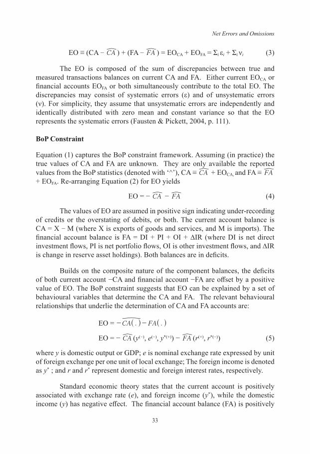
EO ≡ (CA − CA[) + (FA − FA\) = EOCA + EOFA = Σi εi + Σi νi (3)

The EO is composed of the sum of discrepancies between true and measured transactions balances on current CA and FA. Either current EOCA or financial accounts EOFA or both simultaneously contribute to the total EO. The discrepancies may consist of systematic errors (ε) and of unsystematic errors (ν). For simplicity, they assume that unsystematic errors are independently and identically distributed with zero mean and constant variance so that the EO represents the systematic errors (Fausten & Pickett, 2004, p. 111).

BoP constraint

Equation (1) captures the BoP constraint framework. Assuming (in practice) the true values of CA and FA are unknown. They are only available the reported values from the BoP statistics (denoted with ‘^’), CA ≡ CA[ + EOCA, and FA ≡ FA\ + EOFA. Re-arranging Equation (2) for EO yields

EO = − CA[ − FA\ (4)

The values of EO are assumed in positive sign indicating under-recording of credits or the overstating of debits, or both. The current account balance is CA = X − M (where X is exports of goods and services, and M is imports). The financial account balance is FA = DI + PI + OI + ∆IR (where DI is net direct investment flows, PI is net portfolio flows, OI is other investment flows, and ∆IR is change in reserve asset holdings). Both balances are in deficits.

Builds on the composite nature of the component balances, the deficits of both current account −CA and financial account −FA are offset by a positive value of EO. The BoP constraint suggests that EO can be explained by a set of behavioural variables that determine the CA and FA. The relevant behavioural relationships that underlie the determination of CA and FA accounts are:

EO = . .CA FA- -^ ^h h\EO = − CA[(y(−), e(−), y*(+)) − FA\(r(+), r*(−)) (5)

where y is domestic output or GDP; e is nominal exchange rate expressed by unit of foreign exchange per one unit of local exchange; The foreign income is denoted as y* ; and r and r* represent domestic and foreign interest rates, respectively.

Standard economic theory states that the current account is positively associated with exchange rate (e), and foreign income (y*), while the domestic income (y) has negative effect. The financial account balance (FA) is positively

Tang Tuck Cheong

34

explained by domestic interest rates (r), but negatively related to foreign

interest rates (r*). It summarizes that, 0dydEO

dydCA 2=-[

, 0dedEO

dedCA 2=-[

,

0dydEO

dydCA

* * 1=-\

, 0drdEO

drdFA 1=-\

, and 0drdEO

drdFA

* * 2=\

. Both y, e and r*

variables are expected to have a positive impact on a country’s EO by either current account or financial account. The y* and r have negative impact on EO.

open economy macro equilibrium: income-expenditure Approach

An alternative approach to derive the EO equation is by the general equilibrium perspective of two-sector open economy, namely income-expenditure approach. It ‘complements’ the former approach which is essentially based on accounting relationships by incorporating relevant structural relationships. From national income-expenditure approach the CA balance (CA) is equivalent to the national saving (Sn) minus investment (I) balance

CA = Sn − I (6)

In a closed economy, total national savings is fully utilised to domestic investment. But, in an open economy, national saving can be invested at home or abroad that the relationship between savings and investment can be rewritten as Sn = Id + I f where If ≡ CA = −FA. Foreign investment (I f ) is reflected in the acquisition of foreign assets (FA < 0) and commensurate transfers of domestic real resources to users abroad (CA > 0) (see, Fausten, 1989–90). The two main component accounts (CA and FA) of the BoP enter into the relevant market clearing conditions of an open economy. The CA balance represents the excess supply of domestic output (real sector) while the balance on FA reflects the excess demand for assets (financial sector) (see Tang & Fausten, 2012, p. 236).

The structure of this interdependency is conceptually informed by the recognition that any economic disturbance and its response are not restricted to a particular subset of markets (Tang & Fausten, 2012, p. 230). All transactions in goods and services are mediated by financial instruments of one kind or another. In view of the interdependence between the CA and FA accounts, Equation (4) in Fausten and Pickett (2004, p.111) can be rewritten as Sn − I = CA ≡ CA[ + EO = −FA ≡ −(FA\ + EO). They have conceptually introduced some macroeconomic structure such as savings-investment balance into the EO determination, but no further empirical work. They have raised a concern that “Since that type of reduced form does not discriminate between the alternative interpretations of the saving-investment balance it is unlikely to isolate the dominant source of E&O (errors and omissions)” (Fausten & Pickett, 2004, pp. 111−112). Accordingly, the

Net Errors and Omissions

35

estimated parameters of Sn and I are not adequately explaining the ‘emotions’ of EO. At least, the so-called ‘interpretations’ issue can be handled by modelling the behaviour of SnY(.) and IU(.) from the general equilibrium perspective i.e. income-expenditure approach, for example. Substituting Equation (6) onto Equation (4) yields EO = −SnY(.) + IU(.) −FA\(.). The requirements in the goods market suggest that EO can be explained by a set of behavioural variables that determine national saying (Sn), private investment (I), and FA. The relevant behavioural relationships that underlie the determination of national saying, private investment, and financial account are depicted in Equation (7).

EO = −SntY(y(+), r(+)) + IU(r(−)) − FA\(r(+), r*(−)) (7)

Fundamental economic theory suggests that national saving (Sn) is positively explained by households’ disposable income (y), and domestic interest rate (r). Meanwhile, domestic investment (I) is negatively related to domestic interest rate (r), and the financial account balance (FA) is positively explained by domestic interest rate (r), and negatively related to foreign

interest rate (r*). Their associations can be communicated as 0dydEO

dydSn1=-

X,

0drdEO

drdS

drdI

drdFAn

1=- = =-X \

, and 0drdEO

drdFA

* * 2=-\

. Both y and r has

negative impact on a country’s ‘net errors and omissions’, while the r* has positive sign.

emPiricAl illustrAtioN

This section reports the estimates of two EO equations with the Australian data including the graphical presentation of non-causality tests. The sample covers quarterly observations between 1960Q1 and 2010Q2. The core variables are described as follows.

i. Net errors & omissions, lnEO: The data are obtained from OECD Main Economic Indicators. It is reported in local currency A$ (in billions). Nominal values are converted into real term by GDP deflator. The ‘ln’ is natural logarithm (a constant value is added to ensure positive values).

ii. Real GDP, lny: The data are directly collected from International Financial Statistics, IMF, GDP volume constant prices (A$, in billions).

iii. Real interest rate, r: It is the Australian long-term government bond yield (% p.a). Real interest rate is adjusted by domestic inflation rate. The data source is similar to (ii).

Tang Tuck Cheong

36

iv. Real exchange rate, lne: It is quoted as US$ per A$. Nominal exchange rate is multiplied by a price ratio, Australia’s GDP deflator per U.S.’s GDP deflator. The raw data are obtained from International Financial Statistics, IMF.

v. Foreign real interest rate, r*: Same as calculation in (iii). The “foreign” interest rate is proxied by U.S. long-term government bond yield. Nominal values are converted into real terms by US inflation rate. The data are collected from the source as in ii.

vi. Foreign real GDP, lny*: As noted in (v), the “foreign” is U.S. The data of US GDP volume constant prices are directly obtained from International Financial Statistics, IMF.

In the first place, Phillips and Perron (PP) unit root test (Phillips & Perron, 1988) suggest lnEO is stationary in level, I(0) as well as by the ‘minimise ADF test’ for structural break (i.e. 1984Q4). But, other variables are non-stationary, I(1) as informed by the PP test.9 Since the dependent variable, lnEO is I(0), the Equations (5) and (7) are not in favour for cointegration testing while possible cointegrating relation(s) can be occurred among the variables such as growth equation (i.e. lny- r-lne) exchange rate equation (i.e. lne –lny –r –r* –lny -lny*), and so on, but they are not in the present interest on net errors and omissions, lnEO. Perhaps, first differed variables for stationary transformation will result information loss. Hence, OLS linear estimator (non-cointegration case) and multivariate Granger non-causality approach are employed for the data in level.

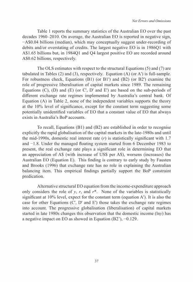
Table 1 Summary statistics for the Australian net errors & omissions, 1960Q1–2010Q2 (in A$ billions)

Mean −0.05Median −0.04Maximum 0.62Minimum −1.65Standard Deviation 0.35Skewness −0.88Kurtosis 6.02Jarque-Bera (Probability) 102.36 (0.00)Observations 202

Net Errors and Omissions

37

Table 1 reports the summary statistics of the Australian EO over the past decades 1960–2010. On average, the Australian EO is reported in negative sign, −A$0.04 billions (median), which may conceptually suggest under-recording of debits and/or overstating of credits. The largest negative EO is in 1986Q1 with A$1.65 billions but, in 1984Q1 and Q4 largest positive EO are recorded around A$0.62 billions, respectively.

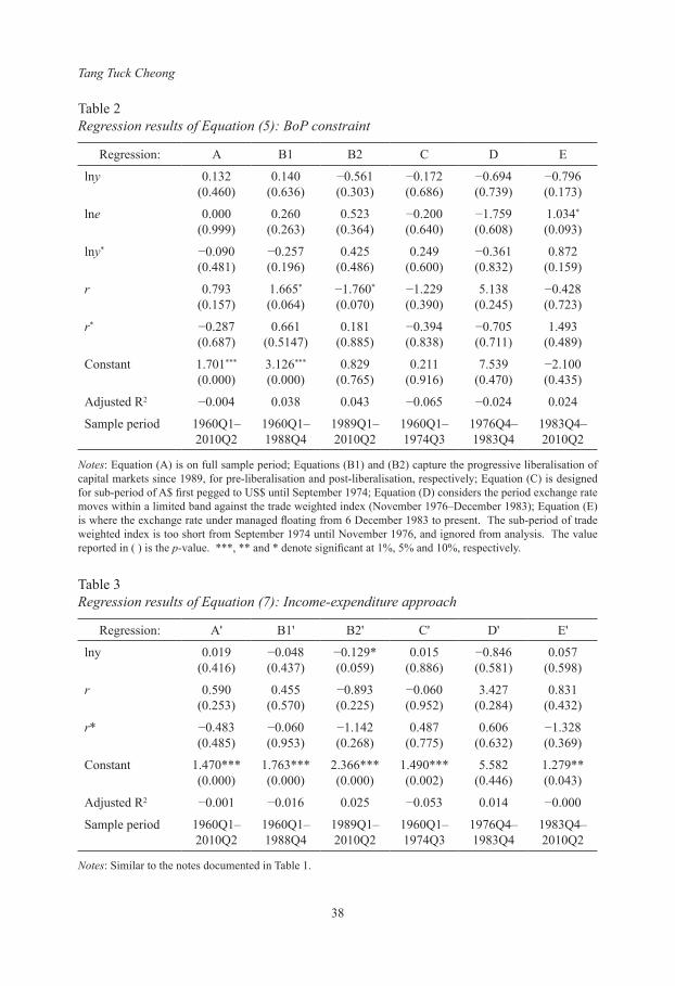
The OLS estimates with respect to the structural Equations (5) and (7) are tabulated in Tables (2) and (3), respectively. Equation (A) (or A') is full-sample. For robustness check, Equations (B1) (or B1') and (B2) (or B2') examine the role of progressive liberalisation of capital markets since 1989. The remaining Equations (C), (D) and (E) (or C', D' and E') are based on the sub-periods of different exchange rate regimes implemented by Australia’s central bank. Of Equation (A) in Table 2, none of the independent variables supports the theory at the 10% level of significance, except for the constant term suggesting some potentially unidentified variables of EO that a constant value of EO that always exists in Australia’s BoP accounts.

To recall, Equations (B1) and (B2) are established in order to recognise explicitly the rapid globalisation of the capital markets in the late-1980s and until the mid-1990s, domestic real interest rate (r) is statistically significant with 1.7 and −1.8. Under the managed floating system started from 6 December 1983 to present, the real exchange rate plays a significant role in determining EO that an appreciation of A$ (with increase of US$ per A$), worsens (increases) the Australian EO (Equation E). This finding is contrary to early study by Fausten and Brooks (1996) that exchange rate has no role in explaining the Australian balancing item. This empirical findings partially support the BoP constraint predication.

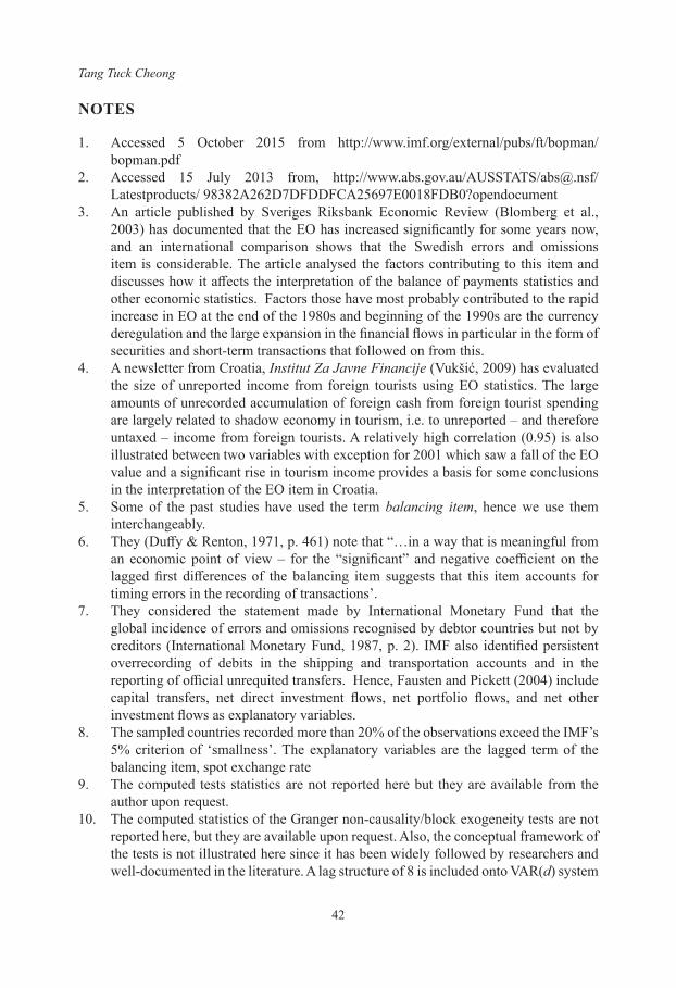
Alternative structural EO equation from the income-expenditure approach only considers the role of y, r, and r*. None of the variables is statistically significant at 10% level, expect for the constant term (equation A'). It is also the case for other Equations (C', D' and E') those takes the exchange rate regimes into account. The progressive globalisation (liberalisation) of capital markets started in late 1980s changes this observation that the domestic income (lny) has a negative impact on EO as showed in Equation (B2’), −0.129.

Tang Tuck Cheong

38

Table 2 Regression results of Equation (5): BoP constraint

Regression: A B1 B2 C D E

lny 0.132(0.460)

0.140(0.636)

−0.561(0.303)

−0.172(0.686)

−0.694(0.739)

−0.796(0.173)

lne 0.000(0.999)

0.260(0.263)

0.523(0.364)

−0.200(0.640)

−1.759(0.608)

1.034*

(0.093)

lny* −0.090(0.481)

−0.257(0.196)

0.425(0.486)

0.249(0.600)

−0.361(0.832)

0.872(0.159)

r 0.793(0.157)

1.665*

(0.064)−1.760*

(0.070)−1.229(0.390)

5.138(0.245)

−0.428(0.723)

r* −0.287(0.687)

0.661(0.5147)

0.181(0.885)

−0.394(0.838)

−0.705(0.711)

1.493(0.489)

Constant 1.701***

(0.000)3.126***

(0.000)0.829

(0.765)0.211

(0.916)7.539

(0.470)−2.100(0.435)

Adjusted R2 −0.004 0.038 0.043 −0.065 −0.024 0.024

Sample period 1960Q1–2010Q2

1960Q1–1988Q4

1989Q1–2010Q2

1960Q1–1974Q3

1976Q4–1983Q4

1983Q4–2010Q2

Notes: Equation (A) is on full sample period; Equations (B1) and (B2) capture the progressive liberalisation of capital markets since 1989, for pre-liberalisation and post-liberalisation, respectively; Equation (C) is designed for sub-period of A$ first pegged to US$ until September 1974; Equation (D) considers the period exchange rate moves within a limited band against the trade weighted index (November 1976–December 1983); Equation (E) is where the exchange rate under managed floating from 6 December 1983 to present. The sub-period of trade weighted index is too short from September 1974 until November 1976, and ignored from analysis. The value reported in ( ) is the p-value. ***, ** and * denote significant at 1%, 5% and 10%, respectively.

Table 3Regression results of Equation (7): Income-expenditure approach

Regression: A' B1' B2' C' D' E'

lny 0.019(0.416)

−0.048(0.437)

−0.129*(0.059)

0.015(0.886)

−0.846(0.581)

0.057(0.598)

r 0.590(0.253)

0.455(0.570)

−0.893(0.225)

−0.060(0.952)

3.427(0.284)

0.831(0.432)

r* −0.483 (0.485)

−0.060(0.953)

−1.142(0.268)

0.487(0.775)

0.606(0.632)

−1.328(0.369)

Constant 1.470***(0.000)

1.763***(0.000)

2.366***(0.000)

1.490***(0.002)

5.582(0.446)

1.279**(0.043)

Adjusted R2 −0.001 −0.016 0.025 −0.053 0.014 −0.000

Sample period 1960Q1–2010Q2

1960Q1–1988Q4

1989Q1–2010Q2

1960Q1–1974Q3

1976Q4–1983Q4

1983Q4–2010Q2

Notes: Similar to the notes documented in Table 1.

Net Errors and Omissions

39

multivariate vAr Granger Non-causality

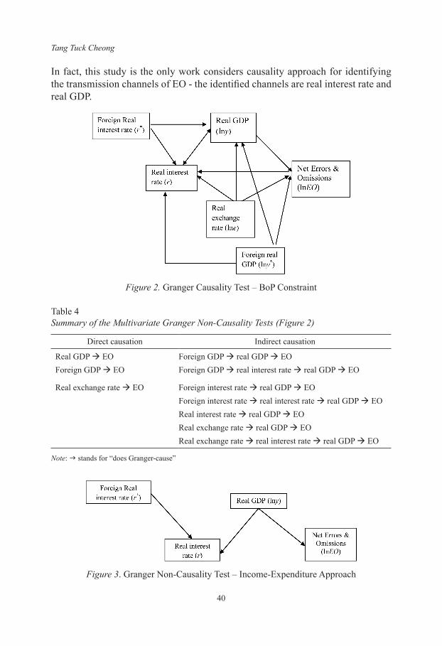
The empirical investigation is extended to the Granger non-causality tests. Non-causality tests help to identify the possible linkages or transmission channels among the variables − in Granger’s reading, “the X causes Y”. According to Granger (1988, p. 200), the cause occurs before the effect, and the causal series contains special information about the series being caused that is not available in the other available series. A multivariate VAR(8) system is employed in which taking all variables into account, simultaneously i.e. lnEO, lny, lne, lny*, r and r*, and lnEO, lny, r and r* for the Equations (5) and (7), respectively.10 For convenient, the findings of Granger non-causality are graphically illustrated in diagrams Figures 2 and 3 for the Equations (5) and (7), respectively.

From the causation patterns observed in Figure 2, they are direct and indirect causation from the macroeconomic variables to EO. Also, their directions of causality are reported in Table 4. The variables y, y*, and e have directly caused the Australian EO. They (y*, and e) and other variables r* and r have indirect causal effect on EO through real sector (i.e. real GDP) and financial sector (i.e. domestic interest rates). Interestingly, the causality tests show that EO does Granger-cause the domestic real interest rate, r. It implies that the past values of EO have relevant information to understand (predict) the current Australia’s interest rate movements.

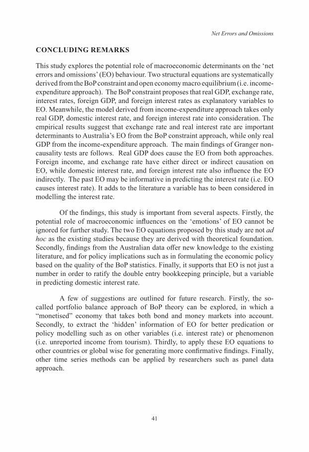
Figure 3 exhibits the causal linkages among r*, r, lny, and lnEO. The Granger-causality results from the income-expenditure approach show only real GDP causes the Australian EO of balance of payment accounts. This appears contrary to the former approach (BoP constraint) that both domestic and foreign interest rates have indirect impact on EO. A causal linkage is found from real GDP to interest rate; and from foreign interest rate to the Australian interest rate.

The ‘old’ variables (from the past studies) such as monetary base, exchange rate (volatility), interest differential, economic openness, and the past EO in explaining the ‘emotion’ of EO, are complemented by two new variables − domestic real GDP (y), and foreign real GDP (y*). The ‘repeated’ variables proposed are exchange rate (e), and domestic and foreign interest rates (r and r*) in which the latter has been implicitly captured by interest differential. In general, the above findings offer a new perspective to the literature. For the two newly introduced variables, the OLS results do support domestic real GDP only based on the income-expenditure approach, but foreign income (real GDP) is statistically insignificant. Meanwhile, exchange rate, and domestic interest rate variables, to some extent are in line with the past studies. By the same token, the causality findings acknowledge the role of exchange rate employed in the past studies.

Tang Tuck Cheong

40

In fact, this study is the only work considers causality approach for identifying the transmission channels of EO - the identified channels are real interest rate and real GDP.

Figure 2. Granger Causality Test – BoP Constraint

Table 4Summary of the Multivariate Granger Non-Causality Tests (Figure 2)

Direct causation Indirect causation

Real GDP à EO Foreign GDP à real GDP à EOForeign GDP à EO Foreign GDP à real interest rate à real GDP à EO

Real exchange rate à EO Foreign interest rate à real GDP à EOForeign interest rate à real interest rate à real GDP à EOReal interest rate à real GDP à EOReal exchange rate à real GDP à EOReal exchange rate à real interest rate à real GDP à EO

Note: stands for “does Granger-cause”

Figure 3. Granger Non-Causality Test – Income-Expenditure Approach

Net Errors and Omissions

41

coNcluDiNG remArKs

This study explores the potential role of macroeconomic determinants on the ‘net errors and omissions’ (EO) behaviour. Two structural equations are systematically derived from the BoP constraint and open economy macro equilibrium (i.e. income-expenditure approach). The BoP constraint proposes that real GDP, exchange rate, interest rates, foreign GDP, and foreign interest rates as explanatory variables to EO. Meanwhile, the model derived from income-expenditure approach takes only real GDP, domestic interest rate, and foreign interest rate into consideration. The empirical results suggest that exchange rate and real interest rate are important determinants to Australia’s EO from the BoP constraint approach, while only real GDP from the income-expenditure approach. The main findings of Granger non-causality tests are follows. Real GDP does cause the EO from both approaches. Foreign income, and exchange rate have either direct or indirect causation on EO, while domestic interest rate, and foreign interest rate also influence the EO indirectly. The past EO may be informative in predicting the interest rate (i.e. EO causes interest rate). It adds to the literature a variable has to been considered in modelling the interest rate.

Of the findings, this study is important from several aspects. Firstly, the potential role of macroeconomic influences on the ‘emotions’ of EO cannot be ignored for further study. The two EO equations proposed by this study are not ad hoc as the existing studies because they are derived with theoretical foundation. Secondly, findings from the Australian data offer new knowledge to the existing literature, and for policy implications such as in formulating the economic policy based on the quality of the BoP statistics. Finally, it supports that EO is not just a number in order to ratify the double entry bookkeeping principle, but a variable in predicting domestic interest rate.

A few of suggestions are outlined for future research. Firstly, the so-called portfolio balance approach of BoP theory can be explored, in which a “monetised” economy that takes both bond and money markets into account. Secondly, to extract the ‘hidden’ information of EO for better predication or policy modelling such as on other variables (i.e. interest rate) or phenomenon (i.e. unreported income from tourism). Thirdly, to apply these EO equations to other countries or global wise for generating more confirmative findings. Finally, other time series methods can be applied by researchers such as panel data approach.

Tang Tuck Cheong

42

Notes

1. Accessed 5 October 2015 from http://www.imf.org/external/pubs/ft/bopman/bopman.pdf

2. Accessed 15 July 2013 from, http://www.abs.gov.au/AUSSTATS/abs@.nsf/Latestproducts/ 98382A262D7DFDDFCA25697E0018FDB0?opendocument

3. An article published by Sveriges Riksbank Economic Review (Blomberg et al., 2003) has documented that the EO has increased significantly for some years now, and an international comparison shows that the Swedish errors and omissions item is considerable. The article analysed the factors contributing to this item and discusses how it affects the interpretation of the balance of payments statistics and other economic statistics. Factors those have most probably contributed to the rapid increase in EO at the end of the 1980s and beginning of the 1990s are the currency deregulation and the large expansion in the financial flows in particular in the form of securities and short-term transactions that followed on from this.

4. A newsletter from Croatia, Institut Za Javne Financije (Vukšić, 2009) has evaluated the size of unreported income from foreign tourists using EO statistics. The large amounts of unrecorded accumulation of foreign cash from foreign tourist spending are largely related to shadow economy in tourism, i.e. to unreported – and therefore untaxed – income from foreign tourists. A relatively high correlation (0.95) is also illustrated between two variables with exception for 2001 which saw a fall of the EO value and a significant rise in tourism income provides a basis for some conclusions in the interpretation of the EO item in Croatia.

5. Some of the past studies have used the term balancing item, hence we use them interchangeably.

6. They (Duffy & Renton, 1971, p. 461) note that “…in a way that is meaningful from an economic point of view – for the “significant” and negative coefficient on the lagged first differences of the balancing item suggests that this item accounts for timing errors in the recording of transactions’.

7. They considered the statement made by International Monetary Fund that the global incidence of errors and omissions recognised by debtor countries but not by creditors (International Monetary Fund, 1987, p. 2). IMF also identified persistent overrecording of debits in the shipping and transportation accounts and in the reporting of official unrequited transfers. Hence, Fausten and Pickett (2004) include capital transfers, net direct investment flows, net portfolio flows, and net other investment flows as explanatory variables.

8. The sampled countries recorded more than 20% of the observations exceed the IMF’s 5% criterion of ‘smallness’. The explanatory variables are the lagged term of the balancing item, spot exchange rate

9. The computed tests statistics are not reported here but they are available from the author upon request.

10. The computed statistics of the Granger non-causality/block exogeneity tests are not reported here, but they are available upon request. Also, the conceptual framework of the tests is not illustrated here since it has been widely followed by researchers and well-documented in the literature. A lag structure of 8 is included onto VAR(d) system

Net Errors and Omissions

43

by given a view that EO is a matter of timing (errors) phenomenon (Tang, 2006b). For the VAR system of lnEO, lny, lne, lny*, r and r*, the LR (sequential modified LR test statistic) suggests 8 lags, while 2 lags by FPE (Final prediction error), AIC (Akaike information criterion), and HQ (Hannan-Quinn information criterion). SC (Schwarz information criterion) suggests 1 lag. The AIC, FPE, and LR suggest 8 lags, while 1 lag by SC and HQ for the VAR system of lnEO, lny, r and r*.

refereNces

Blomberg, G., Forss, L., & Karlsson, I. (2003). Errors and omissions in the balance of payments statistics – a problem? Sveriges Riksbank Economic Review, 2, 41−50. http://www.riksbank.se/Upload/Dokument_riksbank/Kat_publicerat/PoV_sve/sv/2003_2.pdf

Duffy, M., & Renton, A. (1971). An analysis of the U.K. balancing item. International Economic Review, 12(3), 448−464. https://doi.org/10.2307/2525357

Fausten, D. K. (1989–1990). Current and capital account interdependence. Journal of Post Keynesian Economics, 12(2), 273−292. https://doi.org/10.1080/01603477.1989.11489798

Fausten, D. K., & Brooks, R. D. (1996). The balancing item in Australia's balance of payments accounts: an impressionistic view. Applied Economics, 28(10), 1303−1311. https://doi.org/10.1080/000368496327859

Fausten, D. K., & Pickett, B. (2004). 'Errors & omissions' in the reporting of Australia's cross-border transactions. Australian Economic Paper, 43(1), 101−115. https://doi.org/10.1111/j.1467-8454.2004.00219.x

Granger, C. W. (1988). Some recent developments in a concept of causality. Journal of Econometrics, 39 (1-2), 199−211. https://doi.org/10.1016/0304-4076(88)90045-0

International Monetary Fund. (1987). Report on the world current account discrepancy. Washington, DC, September. Retrieved from https://www.imf.org/en/Publications/Books/Issues/2016/12/30/Report-on-the-World-Current-Account-Discrepancy-25

Lin, M.-y., & Wang, H.-h. (2009). What causes the volatility of the balancing item? Economics Bulletin, 29(4), 2749−2759. Retrieved from http://www.accessecon.com/Pubs/EB/2009/Volume29/EB-09-V29-I4-P28.pdf

Phillips, P. C., & Perron, P. (1988). Testing for a unit root in time series regression. Biometrika, 75(2), 335−346. https://doi.org/10.1093/biomet/75.2.335

Tang, T. C. (2005). Does exchange rate volatility matter for the balancing item of balance of payments accounts in Japan? an empirical note. Rivista Internazionale di Scienze Economiche e Commerciali (Now known as International Review of Economics - Journal of Civil Economy), 52(4), 581−590. Retrieved from http://repository.um.edu.my/40623/

Tang, T. C. (2006a). The influences of economics openness on Japan's balancing item: An empirical note. Applied Economics Letters, 13(1), 7−10. https://doi.org/ 10.1080/13504850500119146

Tang Tuck Cheong

44

Tang, T. C. (2006b). Japan's balancing item: do timing errors matters? Applied Economics Letters, 13(2), 81−87. https://doi.org/10.1080/13504850500378718

Tang, T. C., & Fausten, D. K. (2012). Current and capital account interdependence: an empirical test. International Journal of Business and Society, 13(3), 229−244. Retrieved from http://citeweb.info/20081689557

Tombazos, C. G. (2003). New light on the 'impressionistic view' of the balancing item in Australia's balance of payments accounts. Applied Economics, 35(12), 1369−1379. https://doi.org/10.1080/0003684032000129354

Vukšić, G. (2009, May). Croatian balance of payments: Implications of net errors and omissions for economic policy. Institut Za Javne Financije - Newsletter, 41, 1−5. Retrieved from http://www.ijf.hr/eng/newsletter/41.pdf