new modeling techniques for two-piece plunger …
TRANSCRIPT

NEW MODELING TECHNIQUES FOR TWO-PIECE
PLUNGER LIFT COMPONENTS
by
DIVYAKUMAR O. GARG, B.E.
A THESIS
IN
PETROLEUM ENGINEERING
Submitted to the Graduate Faculty
of Texas Tech University in Partial Fulfillment of the Requirements for
the Degree of
MASTER OF SCIENCE
IN
PETROLEUM ENGINEERING
Approved
Chairperson of the Committee
Accepted
Uean ot the Graduate School
December, 2004

ACKNOWLEDGEMENTS
There are many people associated with this thesis deserving recognition. I would
like to thank Dr. James F. Lea for his overall direction, support, and training. I would like
to thank Mr. Joe Mclnemey for setting up the testing equipment and helping me to take
the experimental readings. I would also like to thank Dr. James C. Cox for serving on my
conmiittee and for his guidance.
1 would like to express thanks to family members, friends, and colleagues whose
understanding and support made schooling relatively easier.
Special mention is given to Dr. Akanni Lawal for the support provided by him.

TABLE OF CONTENTS
ACKNOWLEDGEMENTS i
ABSTRACT v
LIST OF TABLES vi
LIST OF FIGURES vii
NOMENCLATURE ix
CHAPTER
I INTRODUCTION 1
1.1 Obj ective of the Proj ect 2
II METHODS OF DE-WATERING GAS WELLS 3
2.1 Sucker Rod Pumps 3
2.1.1 Basics of Sucker Rod Pump 3
2.1.2 The Successive Steps in the Pump Operation 5
2.2 Hydraulic Pumping 7
2.3 Foaming 9
2.4 Gas Lift 11
2.5 Electrical Submersible Pump (ESP) 12
2.6 Progressive Cavity Pumps (PCP) 13
2.7 Velocity Strings 15
2.8 Summary 15
m CONVENTIONAL AND TWO-PIECE PLUNGER BACKGROUND 16
3.1 Plunger Lift 16
3.2 Standard Plunger Operation 17
3.3 Plunger System Equipment 19
3.3.1 Subsurface Equipment - Plungers 19
3.3.2 Down Hole Equipment - Springs and Stops 19
n

3.3.3 Surface Equipment 19
3.3.4 Controllers 20
3.4 Conventional Plunger Cycle Steps 21
3.5 Plunger Lift - Will it Work? 22
3.6 Conventional Plunger Operation 24
3.7 Two-Piece Plunger 25
3.8 Two - Piece Mechanical Components 26
3.8.1 Equipment Description: 26
3.9 Two - Piece Plunger Cycle Steps 27
3.10 Two - Piece Plunger Cycle Concerns 29
IV TWO-PIECE PLUNGER TESTING FACILITY AND TEST PROCEDURE 30
4.1 TestPocedure 32
V RESULTS AND DISCUSSIONS OF TWO-PIECE PLUNGER CASES 33
5.1 Examples: Discussion of Results for Two-Piece Plunger Cases 33
5.1.1 Fall Velocity for Ball 33
5.1.2 Fall Velocity for Hollow Cylinder 3 5
5.1.3 Discussion for Component Fall Velocities 3 6
5.2 Re-plots for Titanium and Steel Two - Piece Plunger Sets 36
5.2.1 Fall Velocity Re-plots for Ball 36
5.2.2 Fall Velocity Re-plots for Hollow Cylinder 38
5.2.3 Discussion - Titanium and Steel Two-Piece Plunger Sets 39
5.3 Lifting of Liquid Slugs 40
5.4 Additional Plotted Model Predictions 41
5.4.1 Titanium Plunger and Ball Set, 6 in. 42
5.4.2 Titanium Plunger and Ball Set, 10 in. 43
5.4.3 Steel Plunger and Ball Set, 6 in. 44
5.4..4 Steel Plunger and Ball Set, 8 in. 45
m

5.4.5 Titanium Plunger and Ball Set, 8 in. 46
5.4.6 Steel Plunger and Ball Set, 9 in. 47
5.4.7 Summary 48
VI SUMMARY: TESTING AND MODELLING FOR THE TWO-PIECE
PLUNGER 49
REFERENCES 51
APPENDIX 56
A DEVELOPMENT OF DRAG EQUATIONS 56
A. 1 Suspension Testing - Drag Coefficient Model 56
A.2 Dynamic Testing - Drag Coefficient Model 60
B CALCULATION OF DRAG COEFFICIENTS OF TWO-PIECE
PLUNGER COMPONENTS 63
B. 1 Drag Coefficient for Ball 63
B.2 Drag Coefficient for Hollow Cylinder 64
B.3 Drag Coefficient for Ball and Cylinder Combined 66
C CRITICAL RATE EQUATIONS 67
D COMPUTER PROGRAM 69
D.I Cylinder Flowrate Code 69
D.2 Fall Velocities Code 70
E EQUATIONS FOR LIFTING OF SLUGS 73
F SAMPLE DATA FOR TWO-PIECE PLUNGER CASES 74
F.l Data for Ball 74
F.2 Data for Hollow Cylinder 81
F.3 Data for Ball and Hollow Cylinder Combined 87
IV
ABSTRACT
The two piece plunger (a steel ball below and a hollow cylinder) seals the tubing
when the ball is on the bottom of the cylinder. The plunger is designed to carry liquids
from a producing gas well to prevent liquid loading. As such it can lift liquids when the
components are together with gas pressure providing the lifting energy. When the two
combined components reach the surface, the liquid is produced and the ball is pushed
away from the cylinder to begin to fall against the flow. The cylinder is retained on the
ball push rod until a short shut-in period of the well. Then the cylinder falls against the
flow and hopefully combines with the ball at the bottom of the well to collect more
liquids in the gas well and carry them to the surface with the combined ball and cylinder.
There are many instances where using this plunger results in production increases.
However in some cases, it appears to have a lesser effect.
Results of testing show that above certain rates, the components will not fall
against the flow in the well. Test results, and the result of drag models to fit the test data
are extended to show the potential user what the allowable rates are from the well, before
the individual components are predicted to fall more slowly or to be unable to fall in the
well, thereby making application impossible without a temporary reduction in the flow
rate. The results should allow the user to be able to better use the two piece plunger in a
wider range of application conditions to remove liquids from a flowing gas well.

LIST OF TABLES
F.I.I Physical Parameters for the titanium ball 74
F. 1.2 Results Extrapolated for titanium ball in Air 74
F. 1.3 Results Extrapolated for titanium ball in Gas (0.65) 77
F.2.1 Physical Parameters for the titanium hollow cylinder 81
F.2.2 Results Extrapolated for titanium hollow cylinder in Air 81
F.2.3 Results Extrapolated for titanium hollow cylinder in Gas (0.65) 84
F.3.1 Physical parameters for the 2 in. titanium set 87
F.3.2.1 Two in. titanium set for 500 fpm fall velocity 88
F.3.2.2 Two in. titanium set for 1000 fpm fall velocity 89
VI
LIST OF FIGURES
2.1 Components of a Sucker Rod pump 4
2.2 Pump Card 5
2.3 Plunger and Ball Valve Details 6
2.4 Jet Pump 8
2.5 Setup for Testing of Foaming Agents 10
2.6 Diagram ofTypical Rotative Gas Lift System 12
2.7 Submersible Pump and Impeller Schematic 13
2.8 Typical PCP Installation 14
3.1 Plunger Lift System 18
3.2 Time Cycle Arrangements 20
3.3 Conventional Plunger Lift Cycle 22
3.4 Feasibihty for a two inch plunger 23
3.5 Two-piece plungers 25
3.6 Mechanical components ofthe Two-piece plunger 27
3.7 Two-piece plunger cycle 28
4.1 Testing Facility at Texas Tech University 31
4.2 Ball suspended in tubing 31
5.1 Critical rates for Titanium Ball 34
5.2 Critical rates for Titanium Cylinder 35
5.3 Titanium Ball Straight Line Plot 37
5.4 Steel Ball Straight Line Plot 37
5.5 Titanium Cylinder Straight Line Plot 38
5.6 Steel Cylinder Straight Line Plot 39
5.7 Titanium Set (Ball and Cylinder) for rise velocity 500 fpm 40
5.8 Titanium Set (Ball and Cylinder) for rise velocity 1000 fpm 41
5.9 Sihca Nitrate Ball, 1 ^ in O.D. and weighs 0.164 lbs 42
5.10 Cylinder 1.9 in O.D and weighs 1.56 lbs 42
5.11 Zircon Ceramic Ball, 1 ' in O.D. and weighs 0.29 lbs 43
Vll

5.12 Cylinder 1.9 in O.D and weighs 2.63 lbs 43
5.13 Zircon Ceramic Ball, 1 '* in O.D. and weighs 0.29 lbs 44
5.14 Cylinder 1.9 in O.D and weighs 2.75 lbs 44
5.15 Steel Ball, l ^ in O.D. and weighs 0.387 lbs 45
5.16 Cylinder 1.9 in O.D and weighs 3.65 lbs 45
5.17 Titanium Ball, 1 '^ in O.D. and weighs 0.23 lbs 46
5.18 Cylinder 1.9 in O.D and weighs 2.125 lbs 46
5.19 Cobah Ball, 1 ' in O.D. and weighs 0.437 lbs 47
5.20 Cylinder 1.9 in O.D and weighs 4.22 lbs 47
A. 1 Schematic Forces on Ball 57
A.2 Schematic Forces on Hollow Cylinder 58
A.3 Schematic forces for Ball and Cylinder combined 59
B.2 Explanation of Variables 64
vui

NOMENCLATURE
a = Outside radius of cylinder, ft
A = Internal tubing diameter, ft
Acir = Clearance area between cylinder and tubing, ft^
A I = Internal area of Cylinder, ft
Ao = Annular area between cylinder and tubing, ft^
Ap = Projected area, ft^
Area = Area ofthe object, ft^
Atbg = Area ofthe tubing, ft^
B = Internal cylinder diameter, ft
Cd = Drag coefficient, dimensionless
Cdcaic - Calculated drag coefficient, dimensionless
Cdmeas - Measured drag coefficient, dimensionless
D = Intemaldiameter ofpipe, ft
Dj = External diameter of cylinder, ft
Di* = Intemaldiameter of cylinder, ft
Do = Internal diameter of tubing, ft
EPT = Effective plunger travel, dimensionless
ESP = Electrical Submersible Pump, dimensionless
f = Friction factor, dimensionless
g(. = Gravitational constant, Ibm-ft /Ibf-sec
GLR = Gas-liquid ratios, scC^Dbl
I.D. = Internal diameter, ft
L = Length of cylinder, ft
m = Mass, lbs
MPT = Maximum plunger travel, dimensionless
O.D. = Outer diameter, ft
p = Pressure, psi
P = Pressure, psi
IX

Pc
PCP
"friction
"weight
Qgcond
Q:
Qm
Qtbg
Qtot
Re
^Gijquid
Slug
Slugiength
t
TbgiD
Vfall
Vgas
Vgcond
Vgwater
'rise
Vt
Vtbg
Wt
z
pair
Pdrag
pimp
a
=,ft
Casing pressure, psi
Progressive cavity pump, dimensionless
Pressure due to friction, psi
Pressure due to column weight, psi
Flow rate of condensate in gas stream, MMscf/D
Flow rate through internal diameter, ft /D
Flow rate through the cylinder in tubing, ft /D
Flow rate in tubing, ft^/D
Total Flow rate through tubing, ft'^/D
Reynolds Number, dimensionless
Specific gravity of liquid, dimensionless
Mass in British gravitational system, -32.17 Ibm
Time, sec
Internal diameter of tubing, ft
Velocity of falling object, ft/sec
In-situ velocity of gas, ft/sec
Velocity of condensate in gas stream, ft/sec
Velocity of water in gas stream, ft/sec
Rise velocity, ft/sec
Critical velocity by Turner, ft/sec
In-situ velocity in tubing, ft/sec
Weight, lbs
Gas deviation factor, dimensionless
Viscosity, Cp
Density of air, Ib/ft
Density of air around object median, lb/ft
Density of air at impact on object, lb/ft
Interfacial tension, dynes/cm

AP = Pressure difference across the object, psi
APcaic = Calculated pressure difference across object, psi
iAPmeas = Mcasurcd pressure difference across object, psi
XI

CHAPTER 1
INTRODUCTION
Forty percent of the wells in the worid are on some kind of artificial lift. For gas
wells, as they deplete liquids often accumulate in the wellbore and the need for artificial
lift arises to lift the hquids from the well. Accumulafion of the liquids in the wellbore is
known as liquid loading, hi mature gas wells, the accumulation of fluids in the well can
impede and sometimes haft gas production. Gas flow is maintained by removing
accumulated fluids using the following most common methods of de-watering of gas
wells:
1) Plunger hft
2) Beam pump
3) Swabbing
4) Soaping
5) Venting the well to atmospheric pressure (blowing down the well)
6) Small tubing (velocity strings or Siphon string)
7) Intermittent gas lift; chamber lift
8) Hydraulic jet or reciprocating hydraulic pump
9) Surfactants
Plunger lift systems have benefits of increasing production, being a cost effective
alternative usually requiring no outside source of energy, which work to reduce the
fallback of liquids slugs as they rise with gas pressure underneath. Continuous removal of
liquids results in higher daily gas production rates than those compared prior to plunger
lift installation The literature " provides background information on conventional
plunger lift operations. In fact, the plunger systems^ also eluninate or reduce frequency of
well treatments required for scale and paraffin removal'^ and remedial treatments such as
swabbing'^ and chemicals. The industry consensuses that plunger lift is one ofthe most
cost effective methods to de-water a gas well.

This research project focuses on a new plunger introduced to the industry. The
plunger constitutes of two separate components (a ball and a hollow cylinder above)
called a two-piece plunger . Combined together the components form a seal of sorts in
the tubing and can allow gas pressure to lift the liquids and the plunger components out
of the well. The components (ball on bottom and cylinder on top) are then controlled to
fall back independently to rejoin at the bottom of the well. The report provides details as
to the equipment used for the testing and the points of caution and concern when using a
two-piece plunger. Drag models to predict the rise and fall of the two individual
components of the new two-piece plunger were developed based upon experimentally
obtained data. Details of the equations used and models developed are provided in the
Appendix A and Appendix B. The results section deals with the cases run and their
discussion. This research project results provide information needed to better, in general,
operate the two-piece plunger systems
1.1 Objective ofthe Project
This research project provides test data and mathematical models to improve
applications of the two-piece plunger. Data was collected on the gas rate required to
suspend the individual components ofthe two-piece plunger; i.e. the ball and the hollow
cylinder both separately and also combined. From this data, by calculating drag
coefficients, models were developed to determine the rise and fall velocities of the ball
and the cylinder as a function of gas rate and pressure. The models developed from
suspension tests were verified by spot checking measured fall velocities with some gas
production taking place. The tests were made using compressed air, but the models
developed allow the calculation of performance in natural gas. The model and charts
developed predict the fall rates for the individual components against a given flow rate
for a given pressure.

CHAPTER 2
METHODS OF DE-WATERING GAS WELLS
This section discusses the most prevalent options in artificial lift methods for
solving the problems of liquid loading as used by the petroleum industry. It provides
briefly a discussion of their method of operation, important features and tables of the
advantages, disadvantages and conditions of applicability of each method.
2.1 Sucker Rod Pumps
2.1.1 Basics of Sucker Rod Pump
Sucker rod pump systems are designed to lift fluids to the surface and are perhaps
the most common methods to remove liquids from gas wells. These systems are applied
when wells do not have enough pressure and gas liquid ratio to allow use of other
methods. The liquid is usually pumped up the tubing and the gas production takes place
from the casing. Beam pump installations have higher installation and operatmg costs as
opposed to other methods such as plunger lift, foaming, or velocity strings. Beam pumps
can work well to remove liquids from a gas well and are hence used in spite of their
comparative high initial and operational costs. Initial costs can be as high as $20,000 -
$60,000 US for placing a typical gas well on rod pump. In addition one can expect to
spend approximately $20,000 US per unit to replace worn downhole pumps and it is
common to pull the pump twice per year (to as low as once in perhaps 4 years) on an
average'^. Attention to problem areas can significantly reduce operating expense. The
components of a sucker rod surface pumping system are illustrated in figure 2.1.

PUMPING UMH \
V
SHEAVES AND BELTS
PRIME MOVER,
CLAMP AND CARRIER BAR
Yy POUSHED ROD t / ^ STUFf rHG BOX
FLOV/ LINE
CASIKQ
TUetNG
SUCKER RODS
TUBING AKa^OR
SINKER BARS
PUMP
GAS AWCHOR
Figure 2.1: Components of a Sucker Rod pump (Courtesy Harbison Fischer)
The pumping unit converts the rotary motion from the prime mover to
reciprocating motion. The prime mover is generally an electrical motor. A good
installation for a sucker rod pumping unit would have an energy efficiency of about 50
percent with efficiency being defined as the energy used to pump the fluids divided by
the energy provided to the installation. The downhole pump is required to handle some
free gas; performing the function of a liquid pump plus a gas compressor. The work on
the fluid done per cycle may be determined from the area of the pump card which is a
plot of the calculated rod loads and position above the pump made each cycle of the
pump. An important tool for diagnosing beam pump problems is the surface
dynamometer card. A surface dynamometer card is the plot ofthe measured or predicted
rod loads at the various positions throughout a complete sfroke. The load is usually

displayed in pounds of force and the position is usually displayed in inches. The pump
dynamometer card is a plot of usually calculated loads at various positions of pump
stroke and represents the load the pump applies to the bottom of the rod string.
Identifying how the pump is performing and analysis of down-hole problems is one ofthe
primary uses of the pump dynamometer card. An example pump card is shown in figure
2.2.
Since the objective is to pump liquids without gas interference, use of a good
downhole gas separator is recommended to prevent gas lock conditions and low
volumetric efficiency in the pump. From the pump card problems such as leaky traveling
or standing valve, tight stuffing box, tubing anchor slipping, gas locked pumps, and
spacing can be diagnosed. Design considerations are available in the literature'^'''* .During
the pumping cycle the gas bubbles in the liquid tend to rise to the top of the pump. At
slow pumping speeds, this separation of gas and liquid may be complete; or in handling
"foamed" fluids, it may be negligible.
Often small amounts of liquid must be produced to allow gas to flow. When a
beam pump is operated at a rate at a rate beyond the capacity of the reservoir to produce
liquids, the liquid level in the well is pumped below the pump intake and the pump is said
to pump-off Considerable literature'^'"^ exists concerning beam pump systems on pump
off control.
2.1.2 Pump Operation Steps
Figure 2.2: Pump card

In figure 2.2 the maximum plunger travel, MPT, is the maximum length of the
plunger movement with respect to the pump barrel during one complete stroke. The fluid
load is a force caused by differential pressure acting on the pump plunger. The
differential pressure acts across traveling valve on the upstroke and is transferred to the
standing valve on the down stroke. The differential pressure is the difference between the
pressure due to the tubing fluids and the pressure in the wellbore. The magnitude of the
fluid load is equal to the pump discharge pressure minus the pump intake pressure
multiplied by the plunger area. From points B to C the rods carry the fluid load, while the
traveling valve is closed. From points D to A the tubing carries the fluid load, while the
standing valve is closed. The effective plunger travel, EPT, is the length of the plunger
travel when the full fluid load is acting on the standing valve. A schematic of plunger and
ball valve details are shown in figure 2.3.
Sucking Rod
Plunger
Well Casing
Riding Valv« Inlets
Standing Valve
Figure 2.3: Plunger and ball valve details 14
There are many kinds of surface units, rods, downhole pumps and other components of
the beam pumping system. The surface units are rated for torque developed by the gear
box, maximum load at the carrier bar, and stroke length. For instance a 456-305-144 unit
can develop 456,000 inch-lbs of torque from the gear box, carry a maximum load of

30,500 Ibfs. and has maximum stroke length of 144 inches of stroke. The rods are rated
with a minimum tensile value that is used to determine the fatigue loading of the rods.
For instance a grade D rod has a minimum tensile rating of 115,000 psi. The main
variable for design for the downhole pump is the diameter that determines the amount of
fluid lifted on each cycle. The motor must provide the energy to move the unit, and
overcome friction in the unit as well as starting torque.
2.2 Hydraulic Pumping
Hydrauhcally powered down-hole pumps are powered by a stream of high-
pressure water or oil (power fluid) supplied by a power-fluid pump at the surface.
Hydraulic downhole pumps are of two types.
1) Piston pumps, which are similar to beam pumps.
2) Jet pumps that operate by power fluid passing through a Venturi, exposing the
formation to low pressure at the outlet of a nozzle or jet. Pressure is recovered as
the jet passes into a throat and then into a diffuser. Then the high pressure fluid is
allowed to produce to the surface.
The surface power-fluid pump usually is a piston-type or centrifugal high-
pressure pump. The power fluid transfers the power necessary to lift liquids from the
surface to the bottomhole pump. The literature ' ' discusses the features of hydraulic
pumping and how it may be applied to de-watering gas wells. The figure 2.4 shows a
typical jet pump with a power fluid being supplied down tubing and production and
power fluid commingling and returning to the surface through the casing annulus.

Power fluid
Co-n'i<igied fluid
Well Rind 2
1
Vlj
HI
|HH'j|n
MHHBHBBBK f
Figure 2.4: Jet Pump. (Courtesy Schlumberger)
Hydraulic pumps can be used to remove liquids from gas wells and are not limited
by depth. They can tolerate a wide range of operating conditions and jet pumps only
handle sand laden or abrasive fluids. Fairly high rates of production are possible.
Jet pumping does require high power for the production achieved or in other words, they
have poor energy efficiency. Jet pumps are capable of handling all forms of fluid
production including gas, steam, or liquid. They are usually installed vertically, but can
be mounted horizontally as well. Reciprocating pumps can lower the formation to lower
values of pressure but can tolerate little solids and less gas than the jet pump.
Reciprocating pumps are much more efficient and may have higher efficiencies than a
beam pump system.

2.3 Foaming
In gas well applications, the liquid/gas/surfactant mixing occurs most commonly
dovm-hole. There are various methods of introducing surfactants into the well. The
simplest method is to batch or continuously inject chemicals down the annulus of a well
with no packer. Also, soap sticks can be dropped down the tubing, manually or with an
automatic dispenser. Surfactant injection can be achieved either down the casing tubing
annulus or through the tubing. Another injection system is one using a capillary tube
lubricated down the tubing to allow injection to depth in flowing wells. Wells are
unloaded with surfactants using two techniques namely batch treatment and continuous
surfactant treatment. Foaming guidelines include the following.
1) Screen foaming agents with lab tests to be sure they will foam well bore fluids.
2) Water is easiest to foam. Condensates are more difficult and require more
expensive chemicals. Water loading is most common problem in the field
operations with most liquid loaded wells being (80-90%) being loaded with
produced and also very commonly loaded with condensed water.
3) If a packer is present, systems exist that allow the lubrication of a 1/4 in. capillary
tube down the tubing to inject chemicals at depth.
4) Soap sticks can be launched down the tubing manually or with various automation
schemes.
5) With no packer, agents can be introduced down the atmulus, either batched or
injected. Consider automated measurements and confrols to schedule treatments.
Foaming is a cheap initial-cost solution for gas-well de-watering, but can be expensive if
large volumes of surfactants are required. Soap sticks are inconsistent and generally fail
to unload the well fully, and when they do unload the well successfully it may be a
shorter term solution. The cost for unloading the well with soap sticks is approximately
$100 US per well each month. It has been used successfully in many appUcations. Some
operators prefer that foams be tried first for liquid-loading problems because they are
inexpensive. The foam produces a less dense mixture by increasing the surface area of
the liquid with bubbles. The result is less gas/liquid slippage. The gas can more easily

carry the foamed liquids to the surface. Foaming is usually possible for liquids if the
liquids contain high percentage of water. Foaming could assist other lift methods for
example plunger lift. The literature^ " ' provides details for foam effect on production of
liquids, foam selection, generation, stability, types of surfactants, correlations, and
laboratory and field testing procedures. Figure 2.5 shows Bureau of Mines setup for
dynamic testing of foaming agents.
FOAV O u t t E !
- O t CD G L - S S ,
24 cm LOfiG
S-r.tHQ HOOKS BtUCH MARK
:-«-—0 6 i.B. h ..ASTJC. 1 4 0 c « , lOfiZ-
i@3
i _ ^ •••MED rRlTTEO CiSC
Figure 2.5: Setup for Testing of Foaming agents 23
10

2.4 Gas Lift
Gas lift introduces additional external gas into the tubing to lighten the flowing
gradient and can increase the fluid velocity above critical rate for the wellbore''^ Critical
rate is a gas rate above which suspended droplets of liquids are predicted to be carried
upward by the gas flow and below critical, droplets are predicted to fall and liquids to
accumulate in the well. Details ofthe equations used for calculating critical rate are given
in Appendix C. A compressor or a high-pressure gas well must supply the lift gas for
gaslift. The usual process is to inject gas down the casing and through a gas lift valve into
the tubing. The gas in the tubing lightens the gradient, and the well produces at a higher
rate. Gas can be injected below the tubing end or injected through only one valve or port
if gas pressure is available to unload. A series of unloading valves can be used to help
inject near the bottom ofthe well with limited gas pressure. The two primary types of gas
lift that are prevalent in the industry are continuous flow and intermittent flow. Gas
cycling is another method to flow additional gas down the annulus and into the bottom of
the tubing ' . A typical gas lift setup with a packer can be seen in figure 2-6.
Gas lift operational guidelines might include the following:
1) Compare costs with other methods.
2) Be sure that compressors and additional gas are available.
3) Model the wells, and possibly the entire field, with gas lift, comparing with other
methods.
Gas lift can be used for high GLR wells and can handle higher sand production than
conventional pumping systems as it is not prone to erosion. It is adaptable to changes in
the reservoir condition and can be used in deviated wells. Changes in the installation can
be made from surface without pulling tubing. The cost of installing a continuous gas lift
system is approximately $30,000 to $50,000 US per well plus the incremental cost of
compression and injection lines.
11
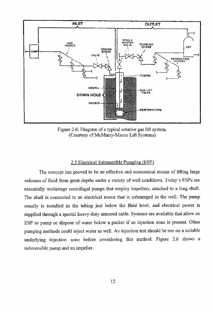
Figure 2.6: Diagram of a typical rotative gas lift system. (Courtesy of McMurry-Macco Lift Systems)
2.5 Electrical Submersible Pumping (ESP)
The concept has proved to be an effective and economical means of lifting large
volumes of fluid from great depths under a variety of well conditions. Today's ESPs are
essentially multistage centrifugal pumps that employ impellers, attached to a long shaft.
The shaft is connected to an electrical motor that is submerged in the well. The pump
usually is installed in the tubing just below the fluid level, and elecfrical power is
supplied through a special heavy-duty armored cable. Systems are available that allow an
ESP to pump or dispose of water below a packer if an injection zone is present. Other
pumping methods could inject water as well. An injection test should be run on a suitable
underlying injection zone before considering this method. Figure 2.6 shows a
submersible pump and an impeller.
12

FI^
£i6etrc
•ack
Sci"s«!tf.ainl»«c
Ey«
Vart6
Figure 2.7: Submersible pump and Impeller Schematic 34
Electrically submersible pumps are generally used for handling large liquid
volumes. They consume more power per barrel than beam pumping systems and their
installation is expensive. The efficiency of this pump system is significantly reduced
when gas is allowed to enter the pump restricting their use for gas well de-watering
operations. The literature ''"^^ refers to the effects of free gas and gas separation and
handling devices in the industry.
2.6 Progressive Cavity Pumps (PCP)
It is of simple design and can handle solids and viscous fluids required for many
operations. They are used for de-watering coal bed methane production, gas wells, and
other water and oil wells. These pumps are preferably used for shallow wells having
13

depth less than 6000 ft. and high fluid rates. The elastomeric stator is vulnerable to
chemical attack and high temperature and many stator rubbers are limited to perhaps 250
degrees F. The literature^ '"*' provides insight into considerations for the components
selection and operational factors, and their troubleshooting. Figure 2.7 shows a typical
PCP setup.
Flow Tee (Gas)'
0^_, Drilled Open Hole o o o o
40 Figure 2.8: Typical PCP Installation
The rotating rods can wear the tubing so centralizers are used. Some advanced
designs employ an ESP motor downhole (ESPPCP). The unit must not pump off as the
PCP pumping only gas can generate very high temperatures in a short time.
14
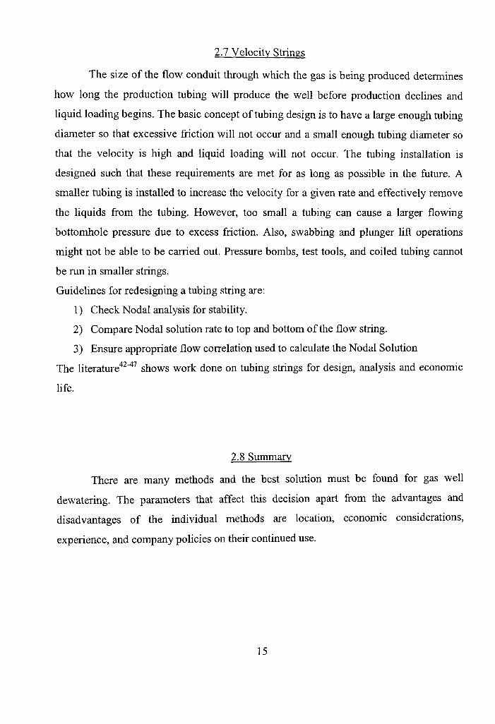
2.7 Velocity Strings
The size of the flow conduit through which the gas is being produced determines
how long the production tubing will produce the well before production declines and
liquid loading begins. The basic concept of tubing design is to have a large enough tubing
diameter so that excessive friction will not occur and a small enough tubing diameter so
that the velocity is high and liquid loading will not occur. The tubing installation is
designed such that these requirements are met for as long as possible in the future. A
smaller tubing is installed to increase the velocity for a given rate and effectively remove
the liquids from the tubing. However, too small a tubing can cause a larger flowing
bottomhole pressure due to excess friction. Also, swabbing and plunger lift operations
might not be able to be carried out. Pressure bombs, test tools, and coiled tubing carmot
be run in smaller strings.
Guidelines for redesigning a tubing string are:
1) Check Nodal analysis for stability.
2) Compare Nodal solution rate to top and bottom ofthe flow string.
3) Ensure appropriate flow correlation used to calculate the Nodal Solution
The literature'' "^^ shows work done on tubing strings for design, analysis and economic
fife.
2.8 Summary
There are many methods and the best solution must be found for gas well
dewatering. The parameters that affect this decision apart from the advantages and
disadvantages of the individual methods are location, economic considerations,
experience, and company policies on their continued use.
15

CHAPTER 3
CONVENTIONAL AND TWO-PIECE PLUNGER - BACKGROUND
3.1 Plunger Lift
The need for plunger lift'"^ operations develops when the natural reservoir
pressure decreases as gases and liquids are produced from the formation. This creates a
condition where the fluids to start collecting in the wellbore, creating a hydrostatic
condition that inhibits the flow ofthe fluids and gases out ofthe formation. The objective
of plunger lift is to keep the immediate vicinity of the wellbore as dry as possible by
lifting liquids on an intermittent basis to the surface. To achieve this when the formation
is producing liquids along with the gas as in natural flow or production, the gas flow must
be of sufficient velocity to deliver all the liquids to the surface in a cyclical manner. The
main reason to remove the liquids from the tubing is so that the pressure on the formation
is reduced as a result of which gas can flow at a higher rate. Also, continual removal of
all produced liquids allows a drying effect on the production formation. This drjdng
effect may actually change in-flow characteristics, giving a well greater capacity for oil
and gas production.
Plunger lift production systems include a cylindrical plunger which travels from a
tubing stop installed as close to the formation as possible to a surface catcher/lubricator.
The plunger travels in reaction time/pressure sequence in order to expel accumulated
fluids into surface facilities. The plunger is designed to provide the necessary interface
between fluid column and the lifting gas. As the plunger is surfacing, gas is leaking or
bypassing around the sides of the plunger, and if excessive, too much energy will be lost
and the plunger will not surface. This prohibits fluid fallback. The volume of fluid above
the plunger should be approximate amount of fluid arriving at the surface although it is
no uncommon for some fluids to follow the plunger.
16

In addition to increased productivity there are other advantages of plunger hft
versus other types of artificial lift . One is the relative inexpensive initial investment and
operating cost compared to sucker rod pumping. Also the advent of automatic electronic
controllers has helped in the removal of much ofthe guesswork associated with a plunger
installation. The automatic electronic controller saves the man hours normally applied
towards fine tuning a plunger system. Finally the plunger can prevent paraffin and scale
buildup from the tubing walls and eliminating costly downtime spent on intermittent
paraffin cleaning. Achieving the continual removal of liquids and gases is dependent
upon the correct installation and operation of plunger lift system. The plunger system
would work well as long as there is sufficient GLR and sufficient pressure along with the
hquid slug. One rule of thumb is that plunger lift requires 400 scf7(bbl-1000ft) but this
does not address the pressure requirement as reservoir pressure is not considered. The
plunger lift systems works satisfactorily with a larger tubing hence there is no need to
dov^Tisize the tubing. The plunger lift works better with no packer or requires wells with
relatively higher formation pressure for the plunger system to work. There might be more
recoverable production with an expensive beam pump system even though the plunger
can take the well to depletion. It has been seen that plunger lift operates successfully to
depths of 20,000 ft and a minimum installation would cost approximately $4000 US.
3.2 Standard Plunger Operation
A typical conventional plunger hft installation^ can be seen in figure 3.1. The
plungers and down hole springs and stops constitute the subsurface equipment. The
surface equipment consists of the lubricator and catcher, the master valve motorized
valve and electronic controllers.
The bumper spring and stop cushions the fall of the plunger at the bottom of the
well. The lubricator and catcher are installed above the master valve of a well and is a
permanent part ofthe wellhead. The lubricator provides an upper Emit for plunger tiravel
and acts as a shock absorber when the plunger reaches the top. The catcher is provided to
17

catch the plunger for inspection or exchange. Once the plunger reaches the top it hovers
between the bleed valve and master valve, wherein a sensor senses the plunger and sends
a magnetic signal to the electronic controller. The electronic controller^ helps to monitor
the plunger cycle by operating the motor valve based upon fluctuations in sales line
pressure, flow rates, pressure differentials, etc. The electronic controller logic based upon
the plunger rise and fall velocities, the casing pressure and possible other form sensor
information.
' LUBRICATOR
FLOW TEE W/O-ntlG
ELECTRONIC CONTROLLER
I'D :2L
PLUM GER
BUMPER SPRHG
Jf^ TUBING STOP
,rr Figure 3.1: Plunger Lift System
18

3.3 Plunger System Equipment
3.3.1 Subsurface Equipment - Plungers
There are a variety of plungers available depending upon the set of well
conditions for which they are to be required. General types of plungers include turbulent
seal brush, wobble washer, expandable blade, multiple turbulent seal, combination
turbulent seal, etc. Also the new two-piece plunger is explained in a following section.
3.3.2 DowTi Hole Equipment - Springs and Stops
The springs and stops are manufactured in various configurations. They serve as
the lower limit to plunger travel and absorb the impact ofthe plunger when it reaches the
bottom of the well. The two pieces of equipment could also be combined into one
assembly consisting of a bumper spring and a standing valve cage, collar lock or tubing
stop. This would make the installation and retrieval easier and less expensive. It also
ensures that the spring stays connected to the stop and doesn't try to flow to the surface
with the plunger.
3.3.3 Surface Equipment
1) Lubricators and Catchers: These are installed above the master valve of an oil or
gas well and become a permanent part of the wellhead. The lubricator serves as
the upper limit for the plunger's fravel and acts as a shock absorber. The catcher,
mounted below the lubricator, is there to manually catch and hold the plunger for
inspection or exchange.
2) Motor Valves: A diaphragm-controlled motor valve is normally included as part
of the surface equipment. They are available for a variety of configurations and
sizes. This includes high pressure, flanged or screwed ends, and severe service.
The motor valve is usually controlled by an electronic controller.
3) Sensors: They detect the arrival of the plunger at the surface, alerting the
electronic controller to activate the proper mode, such as after flow or shut in.
Sensors could be both magnetic and inductive sensors. Magnetic sensors are
19

normally mounted on the catcher nipple, while the new highly sensitive inductive
sensors can be mounted elsewhere
3.3.4 Controllers
The biggest drawback to plunger lift operations is time ad expertise required to
optimize and maintain that optimization. Cycle selection process is generally a time
consuming process that can tie up valuable man hours and require numerous trips to the
well. With continuous changes in sales line pressure, the normal decline of a well,
changing efficiency due to wear of plunger seals, maintaining correct cycles is important.
The electronic controller uses software to create a good window'*^ for most effective
plunger usage. The figure 3.2 below is only one form of logic used for plunger lift
controllers. This particular logic must be further refined to shorted faster cycles for
maximum production.
TIME C Y a E OPERATING WINDOWS:
TIME, urns. 0
FAST ARRlVAt WINDOW
{ LOW TIME )
GOOD ARRIVAL WINDOW
{ HIGH TIME } -
SLOW ^ R i V A L WINDOW
NO ARRIVAL WINDOW
Figure 3.2: Time Cycle Arrangements .48
20

3.4 Conventional Plunger Cycle Steps
The figure 3.3 is a schematic for conventional plunger lift cycle steps.
1) The well is closed in: Pressure builds to needed value to lift the plunger and liquid
slug in the casing. The casing pressure will expand into the tubing and lift the
plunger and associated liquids when the well is opened. If the amount of liquid
present above the plunger is small, then the casing pressure builds to needed value
quicker.
2) Plunger rises: As the plunger rises, a good seal is needed between the plunger and
the tubing ID to prevent gas from bypassing the plunger. A value of about 750
ft/min average velocity during the rise period is often mentioned in the industry as
good practice. Slower results in too much gas slippage and faster results in
friction losses and possible damage to hardware.
3) Plunger surfaces: The liquid above the plunger is produced from the well. It is not
uncommon to detect some liquids following the plunger. The well pressure and
flow hold the plunger at the surface. Gas production commences.
4) Gas produces to lower rates with time: As gas velocity drops with the plunger at
the surface, liquids accumulate in the tubing. This is the concept that as liquids
drop below a critical velocity, liquids are no longer efficiently carried from the
well. The longer the well is allowed to flow at a low rate, the more liquids will
accumulate in the well for the next cycle. It is desirable to keep the liquid slug
size to a small value to optimize production.
5) Plunger falls: From manual or computer controlled signal, the production valve is
closed. For optimum production, the plunger needs to fall fast, collect liquids, and
return when pressure builds to a needed value in the casing. Many conventional
plungers have mechanical devices that open sealing mechanisms or open a
passage though or around the plunger so it will fall faster when the well is closed.
21

(1) Well is closed. Casing pressure is building
t . • '•••""-!
1'-'
1 \
I
•Bii
<3) Gas flows with Plunger at surface.
(2> Valire opens, <4) Liquids accumulate Plunger & »n well as gas velocity liquids rise. slows
(S) Valve shuts & Plunger falls
Figure 3.3: Conventional Plunger Lift Cycle' 49
3.5 Plunger Lift - Will it Work?
Figure 3.4^" refers to a plot that shows the feasibility of a two inch plunger for a
well. This plot is one of the many approximate industry guidelines prevalent in the
petroleum industry to check for plunger feasibility.
Example:
Depth: 8000 ft
Casing buildup pressure in 3 hours: 250 psi
Separator pressure: 50 psi
Net operating pressure: 250 - 50 = 200 psi
22

Result: From chart, about 10,000 scf / bbl for the GLR is needed for plunger operation
from the well. If the well has a lower produced GLR, then the well is considered to NOT
be a candidate for plunger lift. Again this is only an approximate guideline but it does
40000
36000
32000
28000
CQ 24000 m
O CO Q 20000
» 16000
12000
8000
4000
1
ll
1
v\ ^
^•^^^OOOi
2" PLL
DEPTH
f >
NGEER
0 200 400 600 800 1000 1200 1400
NET OPERATING PRESSURE - PSI
Figure 3.4: Feasibility for a two inch plunger 50
include consideration of gas and liquid flow, well pressure, depth and tubing size. It is not
clear from Reference 2 what casing sizes are considered to develop this chart. In general
larger casing is preferred for plunger feasibility.
Note: Another guideline is the there should be a produced well GLR of 400
scf/bbi per 1000 ft of lift. This guideline is an approximate one as it does not consider the
pressure available from the well.
23

3.6 Conventional Plunger Operation
A few important pointers for conventional plunger operation are mentioned below:
1) When a well is flowing at low flow rates it has a tendency to load. This liquid
accumulation in the wellbore increases the backpressure and reduces the
production inflow rate. Thus it is advisable to keep low rate flow periods to short
intervals.
2) To keep the average casing pressure low we should set plunger cycles such that
small amounts of liquid loads are lifted rather than larger loads, thus reducing the
backpressure on the formation and increasing the overall production. This can be
achieved by keeping short build up times.
3) Restiictions in general, such as a choke at the surface reduces plunger and flowing
well performance.
4) The lowest the fluids can flow back into the formation from the wellbore is taken
to be at the last open perforations. This is at times used to push the fluids back
into the reservoir and restart production. If the plunger is below the open
perforation there already is fluid load acting on it. It is hence preferred to keep the
tubing end above open perforations.
5) The plunger weight does not greatly affect the load to be lifted. It is seen that the
plunger weight accoimts up to two percent ofthe total load to be lifted out ofthe
wellbore.
6) The height of a liquid column varies with the cross sectional area of the tubing.
For larger tubing diameter the height ofthe liquid column is lesser than the height
for same amount of liquid tubing with smaller diameter. This helps to reduce the
pressure exerted by the liquid column. Hence a plunger lift may work better in
larger tubing.
7) Since conventional plunger uses the energy of the trapped casing gas it is best to
operate with no packer in the well. When packers are present, higher flowing
wells with a larger buildup pressure are required.
24

.12,51
3.7 Two-Piece Plunger
The plunger'^'^' consists of a hollow cylindrical piston and a ball below. The
hollow cylindrical piston could be changed in length, material used, thickness, size and
number of grooves depending upon usage but is usually a fixed configuration with
various materials available. The ball used along with the hollow cylindrical piston could
also be varied in size and material used but is usually varied only with materials used for
construction. The only consideration is that the ball fits the hollow end of the cylindrical
piston suitably, such that together they appear one piece when joined. The figure below
shows different sizes of plunger. For this report the hollow cylindrical piston along with
the ball would constitute a plunger. Figure 3.5 shows the various types of two-piece
plungers currently being used in the industry.
Figure 3.5: Two-piece plungers'^ (Courtesy MGM Well Services)
The two-piece plunger usage has the following mentioned important features.
These features also suggest why it could be used instead ofthe conventional plunger.
1) The two-piece plunger cycle typically requires only 5 - 1 0 seconds of shut-in
time.
25

2) The ball and the cylindrical piston both fall against a flow rate. This means that
the well is producing, even when the objects are falling to the bottom of the
tubing. This results in more production being obtained from the well.
3) There is a longer flow time as the well is shut-in only for a small time to allow the
cylinder to fall. This leads to the well producing at near about a constant rate.
4) The two-piece plunger does not depend upon the expansion energy of the gas that
is trapped in the casing and tubing annulus but more on velocity and pressure in
the tubing. So even if a there is a packer in the well the two-piece plunger should
function as, it is not dependent on the trapped gas expansion energy. Thus it can
be used with a packer in the hole. In fact, recent field tests show that the two-
piece plunger has been successfiilly used in the field with low flow rate wells
having packers installed from Reference 12.
3.8 Two - Piece Mechanical Components
View figure 3.6 for the mechanical components that are used in the two-piece
plunger. On left is the bottomhole bumper spring. On the right is the spring to cushion
arrival and the shifting rod which holds the cylinder at surface when flow is taking place.
3.8.1 Equipment Description:
The Shifting rod is a downward facing metallic rod. It generally has a taper to it
with a larger diameter towards the bottom ofthe rods. The other mechanical components
have been explained in the system equipment for the conventional plunger.
26

Piston
Ball
Bottom Hole Spring
Lubricator
Surface Springs
Anvil
Shifting Rod
Figure 3.6: Mechanical components ofthe Two-piece plunger'^
3.9 Two - Piece Plunger Cycle Steps
Figure 3.6 shows the various stages involved in the two-piece plunger cycle. The
working ofthe two-piece plunger cycle can be explained by the following points.
1) The figure 3.6 begins with the tubing production automated valve open and the
two-piece plunger sealed with the ball on the bottom of the cylinder bringing up a
slug of liquid.
2) WTien the surface is reached, the cylinder comes over a downward facing rod and
the rod pushes the ball from the bottom of the cylinder and the ball falls (if the
production is not too much). The cylinder remains on the rod while production
flows up between the rod and the I.D. ofthe cylinder. The flow time-period when
the cylinder is at the surface has to be long enough to allow the ball a head start,
or the cylinder will catch it before it reaches bottom.
27
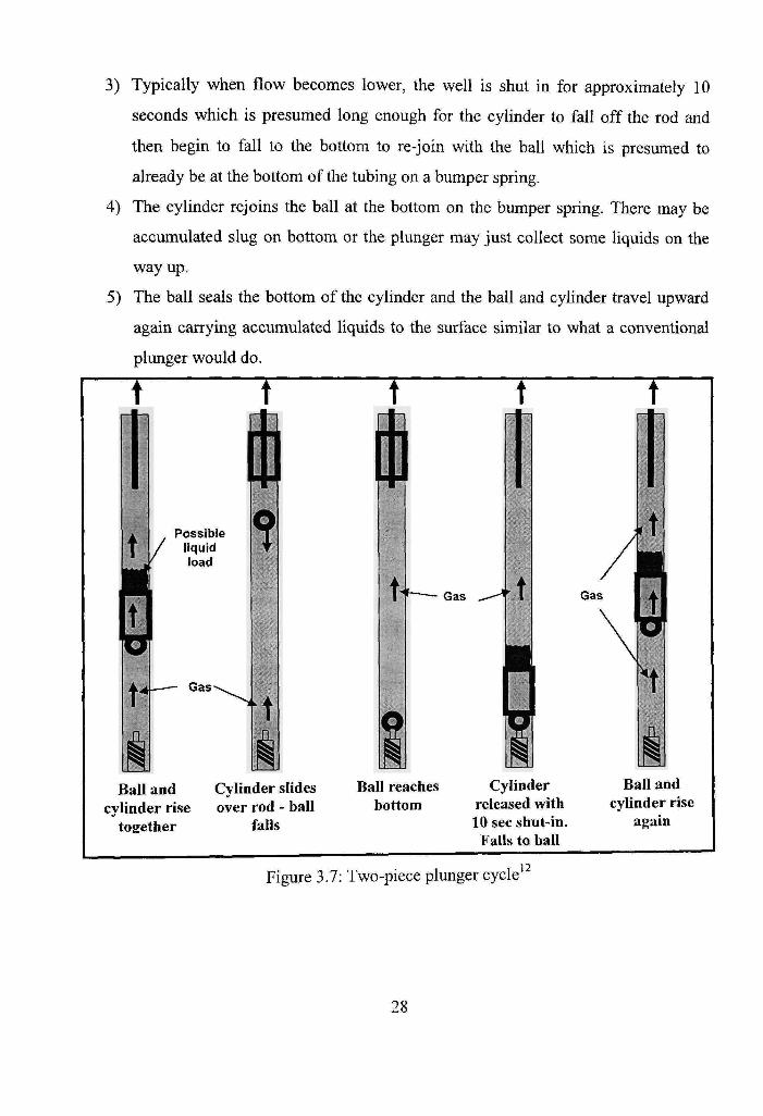
3) Typically when flow becomes lower, the well is shut in for approximately 10
seconds which is presumed long enough for the cylinder to fall off the rod and
then begin to fall to the bottom to re-join with the ball which is presumed to
already be at the bottom of the tubing on a bumper spring.
4) The cylinder rejoins the ball at the bottom on the bumper spring. There may be
accumulated slug on bottom or the plunger may just collect some liquids on the
way up.
5) The ball seals the bottom of the cylinder and the ball and cylinder travel upward
again carrying accumulated liquids to the surface similar to what a conventional
plunger would do.
T T
h-OSSIDK / liquid ' load
f 1 ^
Gas-
t
t Gas
^
Gas
Ball and cylinder rise
together
Cylinder slides over rod - ball
falls
Ball reaches bottom
Cylinder released with 10 sec shut-in. Falls to ball
Ball and cylinder rise
again
Figure 3.7: Two-piece plunger cycle 12
28

3.10 Two - Piece Plunger: Summary of Concerns
1) If the cylinder is released too soon then it could catch the ball before it hits the
bottom. As a result the components would combine above the tubing bottom and
come back up the tubing leaving the liquids below. When the ball and the cylinder
join they act as one body, offering more surface area for flow resistance and
sealing between the liquid and the gas below. This enables the fluid flow to lift
the ball and cylindrical plunger to the surface together.
2) Flow period with the plunger at the surface: If the gas velocity in the tubing has
not dropped to a level below which liquids accumulate in the tubing i.e. below the
critical velocity, the well can be continued to flow with the plunger at the surface
till liquid begins to fall back in the tubing. Even if the gas velocity in the tubing is
above critical velocity the plunger can used. Since the plunger collects droplets
and liquid film up on the way up, it can still cycle effectively as long it collects a
slug on the way up to cushion the arrival. The liquids when lifted to the surface
also help to keep the tubing closer to a dry condition and result in a lower pressure
drop down the tubing and less pressure on the formation, which the goal.
3) Some wells show less response - This could be due to the flow rates not allowing
the components to rejoin near the bottom ofthe well in a reasonable time.
4) Testing was done to determine the fall rates for the components under different
conditions.
29

CHAPTER 4
PLUNGER TESTING FACILITY AND TEST PROCEDURE
The testing to obtain date were conducted at the Texas Tech University,
Petroleum Engineering Department. The equipment used consisted of a horizontal
pressure vessel, a gas compressor with a rating of 125 psig, pipe connections with valve
provisions for fluid inlet at the bottom ofthe tubing, a transparent hardened plastic tubing
of 30 feet in height and a 2 inch tubing diameter according to industry acceptance, and
also pressure gauges at relevant locations. There was also a support structure to facilitate
access to various parts of the tubing. A titanium ball and cylindrical piston set were
initially used. It was an 8 inch titanium plunger and ball set. The titanium ball used was
of 1 3/8* in diameter and weighed 0.218 lbs. The titanium cylindrical piston was of 1.85
inch O.D. and weighed 2.095 lbs. Figure 4.1 shows the testing facility with other
equipment used and figure 4.2 shows the ball suspended in the tubing at the testing
facility.
30

Figure 4.1: Testing Facility at Texas Tech University
Figure 4.2: Ball suspended in tubing
31

4.1 Test Procedure
The air was compressed and stored in the horizontal pressure vessel to provide a
steady source of flow of air through the tubing. By opening the valve the air was
introduced into the tubing. The flow was measured using a flow meter to measure the
amount of gas being flown on a per day basis. At the bottom ofthe tubing the component
of the two-piece plunger was positioned (ball or cylinder) that was to be suspended with
the flow. Once the air was introduced into the tubing, the object was suspended such that
it achieved a steady position, with the object neither rising nor falling in the tubing. The
pressure was read of the respective gauges and the temperature was recorded. The
experiments were repeated until a satisfactory degree of repeatability was obtained. The
object here implies that test runs were made independently for the ball, the cylindrical
piston and the ball and the piston together. Thus in this maimer the weight was equated to
the drag diuing the suspension tests.
The drag model was developed for all the three cases ofthe plunger, firstly for the
ball, secondly for the cylinder and lastly for both the ball and the cylinder together. The
drag model equations are given in details in the Appendix A for all the three cases. The
reason why the three cases needed to be considered was the ball and the hollow cylinder
would fall separately in the hibing, but would rise together as one body while lifting the
fluids out of the tubing. This model was based upon data with specific temperature and
pressure conditions present for air flowing through tubing, was very easily then
extrapolated to different pressures and temperatures using gas of different densities. The
change in the density from air to methane as shown in the results was achieved by simply
using the equation of state. Thus predicted results could be plotted for a gas, as seen in
field conditions, ft is also noteworthy that the drag model for the ball and that for the ball
together with the cylinder were relatively easy to develop.
For the hollow cylindrical piston there were two drag terms to be considered as
flow took place through the inside and as well as the outside of the hollow cylinder. In
fact, to account for the flow rate that took place through the inside and around the
cylinder there is a program code written which has been supplied in the Appendix D.
32

CHAPTER 5
RESULTS AND DISCUSSION OF TWO-PIECE PLUNGER CASES
The results of a few example cases have been shown to better explain the working
of a two-piece plunger. These cases show the fall rate of the component for a given flow
rate and specific pressure. Data was obtained for components falling against a measured
air flow rate as described in the test procedure. The model then extends this data, to
predict the fall velocity of the components, to a gas flow rate natural gas using gas law
relationships. The specific gravity of gas that was used in the calculations was 0.65 and
has been mentioned in the plotted results. The range of fall speed for the components
covers the entire practical and industry preferred velocities. These results show the
operational points for the two-piece plunger. The tabulated data values for the results
which give the pressure, flow rate and component fall speed can be seen in Appendix F.
5.1 Examples: Discussion of Results for Two-Piece Plunger Cases
5.1.1 Fall Velocity for Ball
1) Data: 400 MscfTD production and 200 psi.
Reading the figure 5.1, the ball is predicted to fall at about 1000 Q)m,
which is in accordance with the field observation and hence acceptable. Figure 5.1 gives
the predicted fall rate ofthe ball for a known flow rate and specific pressure. Critical rate
according to Turner's"*^ is also plotted to show minimum flow rate to avoid liquid
loading. If the well has this given pressure and is flowing at mentioned rate, then the ball
when pushed from then end of the cylinder falls to the bottom of the well with the
predicted velocity. This happens as the flow takes place around the falling ball and the
flow rate is insufficient to support the weight ofthe ball. However, at the well surface the
cylinder slides up and over the rod remaining suspended due to the tapered geometry of
33

the rod. This forces more fluid to act on the cross sectional area ofthe cylinder and resists
it's fall. As a result, sufficient time is provided for ball to fall all the way to the bumper
spring and avoid the cylinder to catch up with it mid way in the tubing enabling the
components to rejoin only at the bottom ofthe well and help in removal of accumulated
liquids.
2) Data: 1000 Mscf/D and 500 psi.
Reading figure 5.1, the ball is estimated to fall at a littie more than 200 fpm. This
is fairly slow and it would take 50 minutes to fall in a 10,000' well. If the well is choked
the well back to 600 psi and about 500 Mscf D, then it would fall at about 700 fpm. Then
it would fall back in a 10,000' well in about 15 minutes. If you allow the well to continue
to produce 1 MMscf/D after the ball is dropped, then you must continue to flow with the
cylinder at the surface for 50 minutes. This may be too long for a weak well that is
loosing sfrength and allowing liquids to accumulate as the well falls below the critical
velocity. It might be more desirable to choke the well back to around 600 psi and 500
Mscf/D and then you would only have to flow the well for a minimum of 15 minutes to
insure the ball has reached the bottom before releasing the cylinder.
1000 ,
800 -(S
" • 600 -
j j 400 -
D. ^
200 n
0 -(
Gas(0.65) - Various Vfaii rates for Ball X Q • ^ t ^
\ \ \ \
^^ \ \ \
+ / + / ^ / rh /
\ \ " ^ / - '
• \ \ ^ /
A V A, - ( l i y ,•' — ^ 200fiDm i \ \ \ - ^ / / '"' — • 400fi3m ; V \ ph / / •'' —® eoofjsm
\ I -J _/ y^ •'' — ^ SOOfjam \ 4^ yy'^'* — * lOOOIjDm \^/yy^'' .-.•-.- ofpm
- f c ^ ^ ^ ^ ^ ^ " ' Critical Rates
D 250 500 750 1000 1250 1500 1750 2000
Flow Rates, Mscf/D
Figure 5.1: Critical rates for Titanium ball
34

5.1.2 Fall Velocity for Hollow Cylinder
1) Data: 400 MscCD production and 200 psi.
Reading figure 5.2, this shows the cylinder would fall faster than 1000 fpm and
this is acceptable for most cases. Only the 10 second shut-in would be required to make
sure the cylinder would drop off the downward projecting rod at the surface. It would go
to the bottom in 10 minutes or less in a 10,000 ft well.
2) Data: 1000 MscfiD and 500 psi.
Reading figure 5.2, this shows the cyhnder would fall about 800 fpm. The
cylinder would fall to bottom in 12.5 minutes in a 10,000 ft well. This would probably be
acceptable. You would probably not have to choke the well back to insure the cylinder
would fall at an acceptable rate. The well could continue to flow while the cylinder falls
once it is released from the rod at surface with a 10 sec shut-in.
1000
800
600 Q .
i 400
°- 200
0
Gas(0.65) -Various Vfan Rates of Cylinder + T ^ f .•
-Hi— 200fpm -c,— 400f{3m
eOOfpm -^— 800fpm -o—lOOOfpm -•--- Ofpm --H - - Critical Rates
300 600 900 1200 1500 1800 2100 2400 2700 3000
Flow Rates, Mscf/D
Figure 5.2: Critical rates for Titanium Cylinder
35

5.1.3 Discussion for Component Fall Velocities
In conclusion, it is the ball and not the cylinder which may not fall at desired
velocity against higher flow rates for a reasonably timed cycle of operation. Therefore
considering the above selected data, the well would have to be reduced in flow or choked
back with the cylinder at the surface to insure that the ball reaches bottom to complete an
effective cycle. Then the well could be shut in for a short time to release the cylinder. If
this is not done for higher rates, then the ball will not reach bottom the cylinder will not
reach bottom before recombining with the ball and rising again. This would defeat the
cycle no liquids would be removed from the well. This would not be knovm by the
operator unless careful attention is paid to the well when the cylinder and ball re-surface.
If you drop the ball and cylinder against no flow, then they both fall about 2000
^m. Another option as seen below is to use a ball make of heavier metal.
5.2 Re-plots for Titanium and Steel Two - Piece Plunger Sets
If the plots shown in the above section would be plotted with a change in plot axis
as seen below, then we would obtain plots with straight lines. These straight line plots
would predict the same resuhs as the cross plots above for the exact same data.
In addition to the titanium plunger set in the previous section a straight line plot
for the steel plunger set has also been discussed here.
5.2.1 Fall Velocity re-plots for the Ball
Read figure 5.3. For a flow rate of 500 MscfOD and 100 psi the titanium ball is
falling at a speed of 400 ^m. Now read from figure 5.4. For the same conditions of 500
Mscf/D flow rate and 100 psi the steel ball is falling at a speed of 1400 fpm. Hence the
steel ball falls at a faster rate than compared to the titanium ball.
36

GAS{0,65) - Flow Rate vs Plunger Speed (Ball)
••—lOpsi
- • - 25psi
-*— 50psi
-^^ 75psi
-«-100psi
- ^125ps i
-t—ISOpsi
— 175psi
— 200psi
200 400 600 800 1000 1200 1400 1600 1800 2000
Plunger Speed, fpm
Figure 5.3: Titanium Ball Straight Line Plot
GAS(0.65) - Flow Rate vs Plunger Speed (Ball)
0 200 400 600 800 1000 1200 1400 1600 1800 2000
Plunger Speed, fpm
Figure 5.4: Steel Ball Straight Line Plot
37

5.2.2 Fall Velocity Re-plots for Hollow Cylinder
For a flow rate of 700 Mscf/D reading from Figure 5.5, and at a pressure of 75 psi
the titanium cylinder falls at a speed of 200 fpm. Now examine Figure 5.6. For the same
conditions of 700 Mscf/D flow rate and pressure of 75 psi the steel cylinder falls at a
speed of 1800 fpm.
GAS - Flow Rate vs Plunger Speed (Cylinder)
200 400 600 800 1000 1200 1400 1600 1800 2000
Plunger, fpm
Figure 5.5: Titanium Cylinder Straight Line Plot
38

GAS - Flow Rate vs Plunger Speed (Cylinder)
200 400 600 800 1000 1200 1400 1600 1800 2000
Plunger, fpm
Figure 5.6: Steel Cylinder Straight Line Plot
5.2.3 Discussion - Titanium and Steel Two-Piece Plunger Sets
Titanium is lighter than steel. The total weight of the steel set is significantly
more than that of the titanium set. As seen from the straight line plots above the steel ball
and the steel cylinder fall faster than their respective titanium counterparts on account of
their weight, for same conditions of flow rate and pressure. So, for a well using lighter
equipment (titanium set) we can choke back the well to enable the ball to fall to the
bottom. On the other hand, for higher flow rate wells we can consider using the heavier
equipment (steel set) as they will fall against a higher flow rate than the titanium
components. However, care must be taken not to choke the well below critical for too
long as it might lead to liquid loading the well.
39

5.3 Lifting of Liquid Slugs
Read figure 5.7 and figure 5.8. These figures are plots for predicted rise velocities
of 500 fpm and 1000 fpm ofthe titanium two-piece plunger set for a range of pressures
against a producing well flow rate. The ball and cylinder combine together at the bottom
of the tubing, and rise to lift the liquid slug above them out of the tubing. It is important
to note that the ball and cylinder combine together to rise.. These figures show different
hquid slugs to be lifted, from no slugs to 1 bbl slugs in a gas gravity of 0.65, by the
titanium set. The equations used are given in Appendix E. Currently these appear to be
conservative figures as gas leakage past the plunger greatly aerates the liquid to be lifted
and thus lowering the pressure requirement.
Gas (0.65) - Vrise @ 500 fpm, Bali and Cylinder 500 1
400 ca
°:m
^ 2 0 0 a>
100
200 400 600 800 1000 1200 1400 1600 1800 2000
Flow Rate, IViscf/D
Figure 5.7: Titanium Set (ball and cylinder) for rise velocity 500 fpm
The results are plotted from Foss and Gaul^ model. More work in terms of testing
with a known liquid slug over the plunger set with a measured flow rate could be
performed. The model predicting liquid slug removal could then be developed to agree
reasonably with experimental results with a better understanding of the gas interference
with the hquid slug.
40

Gas (0.65) - Vrise @ 1000 fpm, Bail and Cylinder
0 200 400 600 800 1000 1200 1400 1600 1800 2000
Flow Rate, IWscf/D
Figure 5.8: Titanium Set (ball and cylinder) for rise velocity 1000 fjpm
5.4 Additional Plotted Model Predictions
The physical quantities ofthe two-piece plunger sets, such as the length, diameter
and weight, could be changed resulting in different configurations or two-piece plunger
sets. The difference in weights for same cylinder lengths is directly dependent on material
of construction. Presented below are the results for such different configurations. These
configurations or two-piece plunger sets are those that are currently being used by the
industry. All ofthe following plots give the falling speed ofthe ball and the cylinder for a
given flow rate and operating pressure.
41

5.4.1 Titanium Plunger and Ball Set, 6 in.
GAS(0.65) - Flow Rate vs Plunger Speed (Bal
- ^ 10psi
-*- 25psi
-*r- 50psi
-5<- 75psi
-^•^ lOOpsi
-*- 125psi
-t— 150psi
- ^175ps i
— 200psi
200 400 600 800 1000 1200 1400 1600 1800 2000
Plunger Speed, fpm
Figure 5.9: Silica Nitrate Ball, 1-3/8 in. O.D. and weighs 0.164 lbs
GAS (0.65) - Flow Rate vs Plunger Speed (Cylinder)
-10psl
- 25psi
- SOpsi
- 75psi
-lOOpsI
•125psi
•1 SOpsi
175psl
200psi
200 400 600 800 1000 1200 1400 1600 1800 2000
Plunger, fpm
Figure 5.10: Cylinder 1.9 in. O.D and weighs 1.56 lbs
42

5.4.2 Titanium Plunger and Ball Set, 10 in.
GAS(0.65) - Flow Rate vs Plunger Speed (Ball)
200 400 600 800 1000 1200 1400 1600 1800 2000
Plunger Speed, fpm
Figure 5.11: Zircon Ceramic Ball, 1-3/8 in. O.D. and weighs 0.29 lbs
GAS (0.65) - Flow Rate vs Plunger Speed (Cylinder)
- • - lOpsi
-^<r- 25psi
-c:- 50psi
- e - 75psi
- * -100psi
^•-125psi
-4-ISOpsi
- a - 175psl
200psi
200 400 600 800 1000 1200 1400 1600 1800 2000
Plunger, fpm
Figure 5.12: Cylinder 1.9 in. O.D and weighs 2.63 lbs
43

5.4.3 Steel Plunger and Ball Set, 6 in.
GAS(0.65) - Flow Rate vs Plunger Speed (Ball)
- ^ 1 0 p s i
- * - 25psi
-Tk— SOpsi
- <— 75psi
-K— 10Opsi
- » - 125psi
- I — 1 SOpsi
- ^ 1 7 5 p s i
— 200psi
0 200 400 600 800 1000 1200 1400 1600 1800 2000
Plunger Speed, fpm
Figure 5.13: Zircon Ceramic Ball, 1-3/8 in. O.D. and weighs 0.29 lbs
GAS (0.65) - Flow Rate vs Plunger Speed (Cylinder)
0 200 400 600 800 1000 1200 1400 1600 1800 2000
Plunger, fpm
Figure 5.14: Cylinder 1.9 in. O.D and weighs 2.75 lbs
44

5.4.4 Steel Plunger and Ball Set, 8 in.
200
GAS(0.65) - Flow Rate vs Plunger Speed (Ball)
•^ lOps i
- • - 25psi
-*- SOpsi
-K— 7Spsi
i«— lOOpsi
- ^125ps i
- — ISOpsi
—17Spsi
— 200psi
200 400 600 800 1000 1200 1400 1600 1800 2000
Plunger Speed, fpm
Figure 5.15: Steel Ball, 1-3/8 in. O.D. and weighs 0.387 lbs
GAS (0.65) - Flow Rate vs Plunger Speed (Cylinder)
200 400 600 800 1000 1200 1400 1600 1800 2000
Plunger, fpm
Figure 5.16: Cylinder 1.9 in. O.D and weighs 3.65 lbs
45

5.4.5 Titanium Plunger and Ball Set, 8 in.
GAS(0.65) - Flow Rate vs Plunger Speed (Ball)
- • - lOps i
- • - 25psi
-ifc- SOpsi
- <— 7Spsi
^tf-l00psi
-^125ps i
—i— ISOpsi
^—17Spsi
- — 200psi
200 400 600 800 1000 1200 1400 1600 1800 2000
Plunger Speed, fpm
Figure 5.17: Titanium Ball, 1-3/8 in. O.D. and weighs 0.23 lbs
GAS (0.65) - Flow Rate vs Plunger Speed (Cylinder)
200 400 600 800 1000 1200 1400 1600 1800 2000
Plunger, fpm
Figure 5.18: Cylinder 1.9 in. O.D and weighs 2.125 lbs
46

5.3.6 Steel Plunger and Ball Set, 9 in.
800
700
Msc
f R
ate,
5 o
600
500
400
300
200
GAS(0.65) - Flow Rate vs Plunger Speed (Ball)
-
- - - » -
• • —^—
-^-
'
- • —
'
m— .
1 ' 1 ' ' — • —
1
— • — 1
— • — 1
— i >
-*—10psi
- " - 25psi
-*— SOpsi
-><— 75psi
-^1^ lOOpsi
- • - 125psi
-H— ISOpsi
— 175psi
— 200psi
200 400 600 800 1000 1200 1400 1600 1800 2000
Plunger Speed, fpm
Figure 5.19: Cobalt Ball, 1-3/8 in. O.D. and weighs 0.437 lbs
GAS (0.65) - Flow Rate vs Plunger Speed (Cylinder)
200 400 600 800 1000 1200 1400 1600 1800 2000
Plunger, fpm
Figure 5.20: Cylinder 1.9 in. O.D and weighs 4.22 lbs
47

5.4.7 Summary
From the different predicted situations we see:
1) Consider the 6 in. titanium plunger with the 6 in. steel plunger. For a flow rate of
500 Mscf/D and 50 psi the titanium cylinder falls at 200 fpm. For a 5000 ft. well
the titanium cylinder would travel for 25 min to reach the bottom. For the same
flow rate and pressure the steel plunger falls at a predicted velocity of
approximately 1800 fpm. taking a little under 3 min to travel 5000 ft. Hence, a
heavier two-piece plunger set falls faster when compared to a lighter two-piece
plunger set. Similarly, due to the difference in weights it is seen that the heavier
ball is predicted to fall faster than the lighter ball.
2) The operator can choose the cylinder and ball or a configuration set for the two-
piece plunger based upon the flow rate and time taken by the components to travel
to the bottom. For quicker cycles in a high flow rate well it would do good to use
a heavier set and a lighter set for a weak well.
3) For different configurations a predicted set of ready results is available.
The results plot provide the freedom to choose a specific cylinder and ball to form a
two-piece plunger set to better suit the well conditions and facilitate removal of liquids to
improve production.
48

CHAPTER 6
SUMMARY: TESTING AND MODELLING RESULTS FOR THE
TWO-PIECE PLUNGER
Tests were made in firll scale using real two-piece plungers.
1) Resuhs show operators possible cycle failure modes not previously considered.
2) The Two-Piece plunger may give more production since no build up time, but
components should be allowed to re-join at or near the bottom ofthe well. This
also helps to keep the production rate fairly constant and assists to keep low
bottom hole flowing pressure.
3) Test data and models predict the fall times for the ball and cylinder separately to
help insure operational cycles.
4) If you choke back to allow components to fall, then try to avoid choking back
below critical flow, or don't choke back below critical for too long. However,
choking back probably may not be necessary if you switch to heavier equipment
for higher flow rates.
5) The well continues to produce even when the objects are falling owing to their
clearance areas.
6) A shut-in time of only seconds does not create high spikes in wellhead pressures
or volumes. Thus for a two-piece plunger it is not necessary to oversize the
compressor to accommodate the volume spikes common with the conventional
plunger systems.
7) Two-piece plunger will work wherever a conventional plunger can and has mostly
shown to improve production rate.
8) Results are immediately applicable but may need some adjustment to field
applications
49

9) Companies are now considering longer times to hold the cylinder in place in high
rate application to allow ball to fall as shown necessary by this testing.
10) Future work should include
a. Testing for the effects of adding some bbls of liquid/ MMscf to see effect
of liquids with gas on performance of the two-piece plunger
b. With additional testing with liquids, a computer model of the two-piece
plunger can be developed to help operators set cycle times for various well
conditions for field applications.
50

REFERENCES
1. Lea, J. F.: "Dynamic Analysis of Plunger Lift Operations," Tech. Paper SPE
10253 (November 1982), 2617-2629.
2. Beeson, C. M., Knox, D. G., and Stoddard, J. H.: "Part 1: The Plunger Lift
Method of Oil Production", "Part 2: Constructing Nomographs to Simplify
Calculations", "Part 3: How to User Nomographs to Estimate Performance", "Part
4: Examples Demonstrate Use of Nomographs", and "Part 5: Well Selection and
Apphcations," Pefroleum Engineer (1957).
3. Otis plunger Lift Technical Manual (1991).
4. Ferguson Beauregard Inc Plunger Operation Handbook (1998).
5. Foss, D. L. and Gaul, R. B.: "Plunger Lift Performance Criteria with Operating
Experience-Ventura Field," Drilling and Production Practice, API (1965) 124-40.
6. Phillips, Dan, and Listiak, Scott: "How to Optimize Production form plunger
Lifted Systems, Pt. 2," Worid Oil (May 1991).
7. McCoy, J., Rowlan, L., and Podio, A. L.: "Plunger hft Optimization by
Monitoring and Analyzing Well High Frequency Acoustic Signals, Tubing
Pressure and Casing Pressure," SPE 71083 presented at the 2001 SPE Rocky
Mountain Petroleum Technology Conference in Keystone, Colorado, U.S.A., May
21-23.
8. Hacksma, J. D.: "Users Guide to Predict Plunger Lift Performance," presented at
Southwestern Petroleum Short Course (SWPSC), Lubbock, Texas U.S.A. (1972).
9. Beauregard, E., and Morrow, S.: "New and Unusual Applications for Plunger Lift
System," SPE 18868 presented at the 1989 Production Operations Symposium in
Oklahoma City, Oklahoma, U.S.A., March 13-14.
10. Wang, B., and Dong L.: "Paraffin Characteristics of Waxy Oils in China and
Methods of Paraffin Removal and hihibition," SPE 29954 presented at the 1995
International Meeting on Petroleum Engineering in Beijing, China, November 14-
17.
51

11. Lestz, R.: "Swabbing under Pressure and Flow through Plungers," presented at
the Denver Gas Well De-Watering Workshop (March 2003).
12. Garg, D. et al.: "Two-Piece Plunger Test Results," presented at the SWPSC,
Lubbock, Texas, U.S.A.(19-2I April 2004).
13. Stephenson, G. B., Rouen, R. P., and Rosenzweig, M. H.: "Gas Well De-
Watering: A Coordinated Approach," SPE 58984 presented at the 2000
International Petroleum Conference and Exhibition in Villahermosa, Mexico,
February 1-3.
14. Parker, R.M.: "How to Prevent Gas-Locked Sucker Rod Pumps", World Oil (June
1992), pp. 47-50.
15. Elmer, W., and Gray, A.: "Design Considerations when Rod Pumping Gas
Wells," First Conference of Gas Well De-Watering, SWPSC, Denver (March
2003).
16. Neely, A.B.: "Experience with Pump-Off Control in the Permian Basin," SPE
14345 presented at the 1985 Annual Technical Conference and Exhibition ofthe
SPE, Las Vegas, Nevada, U.S.A., September 22-25.
17. Lea, J.F.: "New Pump-Off Controls Improve Performance," Petroleum Engineer
International (December 1986), pp. 41-44.
18. Clark, K. M.: "Hydraulic Lift Systems for Low Pressure Wells," Petroleum
Engineer International (February 1980).
19. Tait, H.: "Hydrauhc Pumping Systems," presented at the SWPSC, Lubbock,
Texas, U.S.A. (21-22 April 1993).
20. Martin, J. M., and Coleman, W. P.: "hmovative Jet Pump Design Proves
Beneficial in Coalbed Methane De-watering Applications." presented the
SWPSC, Lubbock, Texas, U.S.A. (21-22April 1993).
21. Fretwell, J. A., and Blair, E. S.: "Achieving Low Producing Bottomhole Pressure
in Deep Wells Using Hydraulic reciprocating Pumps," presented at the SWPSC,
Lubbock, Texas, U.S.A. (21-22 April 1999).
52

22. Simpson, D., and Deherrera, W.: "Water Lifting Experiences in the CBM
Fairway," Amoco presentation for Gas Well De-Watering Forum, Farmington,
New Mexico, U.S.A. (1999).
23. Dunning, H.N. et al.: "Foaming Agents for Removal of Liquids from Gas Wells,"
Bull. 06-59-1, American Gas Assoc, New York City.
24. Libson, T.N., and Henry, J.R.: "Case Histories: Identification of and Remedial
Action for Liquid Loading in Gas Wells Intermediate Shelf Gas Play," paper SPE
7467, JPr(April 1980) 685; Trans., AME, 269.
25. Campbell, S., Ramchandran, S. and Bartrip, K.: " Corrosion Inhibitors/Foamer
Combination treatment to Enhance Gas Production," SPE Paper 67325 presented
at the SPE Production and Operations Symposium, Oklahoma City, Oklahoma
(24-27 March 2001).
26. Blauer, R. E., Mitchell, B. J., and Kohlhaas, C.A.: "Determination of Laminar,
Turbulent, and Transitional Foam Flow Losses in Pipes," SPE Paper 4888
presented at the 1974 Annual California Regional Meeting, April 4-5.
27. Jacoby, R. H., NHGPA Phase Equilibrium Project, API Proceedings Division of
Refining (1964), p. 288.
28. Hough, E. W. et al.: "Interfacial Tensions at Reservoir Pressures and
Temperattires; Apparattrs and the Water-Methane System," JPT (1951);Trans.,
AIME, 57.
29. Katz, D. L. et al. Handbook of Natural Gas Engineering, McGraw Hill, New York
(1959).
30. Vosika, J. L.: "Use of Foaming agents to alleviate liquid Loading in the Greater
Green River TFG Wells," SPE/DOE 11644 presented at the SPE/DOE
Symposium on Low Permeablity, Denver (14-16 March 1983).
31. Sloan, R., High Plains Wireline, Elk City, Oklahoma. Waggoner, Richard,
Foamtech, Woodward Oklahoma (1996).
32. Lestz, R.S.: "Capillary Strings to hiject Surfactants," presented at the SWPSC
School on De-Watering Gas Wells, Lubbock, Texas, U.S.A. (24 April 2001).
53

33.Centrilift Submersible Pump Handbook, 6' Edition, Centrilift, Claremore,
Oklahoma (1997).
34. Turpin, J. L., Lea, J. F., and Bearden J. L.: "Gas Liquid Flow through Centrifiigal
Pumps-Correlation of Data," presented at the SWPSC, Lubbock, Texas, U.S.A.
(1986).
35. Centrilift Gas Handling Manual.
36. Dunbar, C.E.: "Determination of Proper Type of Gas Separators," REDA
Technical Bulletin (1989).
37. Wood Group ESP hic. Bulletin on XGC gas separator. Wood Group ESP,
Oklahoma City, Oklahoma (2002).
38. ABB Presentation on World Wide Artificial Lift Statistics by ABB Automation
Technology Products (14 December 2001).
39. Klein, S. T.: "Selecting a Progressive Cavity Pumping System," presented at the
SWPSC, Lubbock, Texas, U.S.A. (20-21 April 1994).
40. Weatherford ALS Progressive Cavity Pump Manual (2001).
41. Griffin Pumps Operators Manual, 5654 55'*' Street, Calgary, S.E., Alberta,
Canada, T2C 3G9.
42. Turner, R.G., Hubbard, M.G., and Dukler, A.E.: "Analysis and Prediction of
Minimum Flow Rate for the Continuous Removal of Liquids from Gas Wells,"
paper SPE 2198, /Fr(November 1969) 1475; Trans., AIME, 246.
43. Coleman, S.B., et al: "A New Look at Predicting Gas Well Liquid Load-Up,"
JPT, (March 1991).
44. Wesson, H. R.: "Coiled Tubing Velocity/Siphon Struig Design and Installation,"
the 1993 Annual Conference on Coiled Tubing Operations and Slimhole Drilling
Practices, Houston, March 1-4.
45. WIS Solutions on "Coiled Tubing Velocity Strings: A Simple, Yet Effective Tool
for the Future Technology," Schlumberger, Dowell.
46. Weeks, S.G.: "Small Diameter Concentric Tubing Extends Economical Life of
High Water-Sour Gas Edwards Producers," SPE 10254 presented at the 1961
54

Annual Fall Technical Conference and Exhibition of SPE of AME, San Antonio,
Texas, October 5-7.
47. Lea, J. F.: "Plunger Lift versus Velocity Strings," Journal of Energy Resources
Technology, Vol. 121 (December 1999), 234-40.
48. Morrow S. J., and Rogers, J. R.: "Increasing Production using Microprocessors
and Tracking Plunger-Lift Velocity," SPE 24296 presented at Mid-Continent Gas
Symposium in Amarillo, Texas, U.S.A. (13-14 April 1992).
49. Lea, J. F.: "Solving Gas-Well Liquid-Loading Problems," SPE 72092,
Distinguished Author Series, JPT (April 2004).
50. Ferguson, P.L., and Beauregard, E.: "How to Tell if Plunger Lift Will Work in
Your Well," World Oil (August 1985), pp.33-37.
51,Bizanti, M.S., and Moonesan, A.: "How to Determine Minimum Flowrate for
Liquid Removal," World Oil (September 1989), pp. 71-73.
55

APPENDIX - A
DEVELOPMENT OF EQUATIONS
This Appendix is divided into two sub sections, both dealing with model
development for calculation of drag coefficients of the two-piece plunger components.
The first section deals with model developed for suspension testing and the second
section deals with dynamic testing. The drag coefficients obtained from both these
models were in agreement, which served the purpose of verifying the validity of the
suspension model and it's results.
A. 1 Suspension Testing - Drag Coefficient Model
Presented here schematically are the forces and the force balance equations that
were considered to calculate drag coefficients. In suspension testing the force balance is
done for the component when it is suspended against a measured flow rate. The
component is freely suspended and there is no acceleration or movement of the
component in either the upward or downward direction.
A. 1.1 Suspended Drag Model for Ball
The direction of forces acting on the ball can be seen in figure A. 1
Equating the drag to weight we get the following equation:
2*g^*l44
Solving for Vgas it is possible to plot the results from the following equation
nO.5
Vgas = {Wt/Area)*2*gc*l44
^" Pimp Vfall. ...(A.2)
56

Weight
Drag
Figure A. 1: Schematic Forces on Ball
A. 1.2 Suspended Drag Model for Hollow Cylinder
The direction of forces acting on falling hollow cylinder can be seen in figure A.2.
Drag forces are seen on the inside and outside of the cylinder due to the gas flow and also
at the bottom surface of the cylinder due to impact.
The equation for cylinder is a bit more complex. For the hollow cylinder equate
impact and longitudinal drag to weight. Pressure drop across the cylinder due to flow
through the hollow cylinder and outside (annular area between the cylinder and tubing)
the cylinder is the same. It was found that the flow through the cylinder accounted for
mostly the entire pressure drop. So the overall drag for the cylinder is given by impact
term and the longitudinal drag on the inside as seen from the equation below.
2*gc *144 ID, *g,*UA*\Ai * Pdrag Y^i Pdrag)
. . .(A.3)
57

Figure A.2: Schematic of Forces on Hollow Cylinder
Let, A Cd* Pimp ^ „ Pdrag* f'^L*{Atf, * Pi )
^—; and B = f z :r 2*g^*144 2*Di *g,*144*(4- * Pdrag?
Rearranging the terms we get,
{Vgas + Vfallf *A + {Vgas + Vfallf * B = 1.43411
Solving for Vgas below, we can plot the results.
Thus, Vgas = 1.43411
A + B
0.5
- Vfall.
..(A.4)
...(A.5)
...(A.6)
58

Note: The suspension test gave the necessary flow rate required to suspend hollow
cylinder in the tubing. Based on the program giyen in Appendix D.l it was established
that almost all (99.5 percent) ofthe flow was taking place through the cylinder. Usmg the
fact a model for the drag internal to the cylinder was developed. The drag on the inside
and the outside ofthe cylinder necessarily has to give identical pressure drops.
A. 1.3 Suspended Drag Model for Ball and Cylinder Combined
Figure A.3 shows the explanation ofthe various forces that are acting on the ball
and cylinder combined.
Drag = TiD^i^^
Gas
PxA Do
Tubing
Ball/Cylinder
Rising
Weight of cylinder
&ball
PxA Pressure below
Ball and Cylinder Rising
Figure A.3: Schematic forces for Ball and Cylinder combined
The ball and the cylinder when combined together constitute a single body. When
combined gas flow took place around the cylinder through the annular area between the
59

outside ofthe cylinder and the inner tubing diameter. For the force balance equation the
impact and the outside drag were equated to the weight. The laminar flow equation was
used for the outside drag based upon calculation of Reynolds number showing value of
less than 2000. The Reynolds number was calculated based on the drag from the flow
rate, outside the ball, required to suspend the combined ball and cylinder.
The force balance equation for the ball and cylinder combined is given as,
Cd * Pimp* (Vgas +Vfall f , (Vgas+Vfall)*8^*A,i, ^^^^TTTJ'A + f ; V^ = Wt/Area ... (A.7) 2 * g , *144
Cd * Pimp
2 * g *144
. - - 6 - ('='-''')' ln{a/b)
8juL * A^i^
*144
a —b \n{alb)
= 144
and C = Vlij {A)+ F^ (2 A * Vf^ii +B)+C = 0 fall \^'^ ' fall \^^ " fall^^r^-^ • • • (^-8)
Rearranging the terms and solving for the equation below, results for Vgas were plotted
andF|^,(^) + Fg«,(2^*F^,„+5)+C = 0 . ...(A.9)
A.2 Dynamic Testing - Drag Coefficient Model
In dynamic testing the acceleration term is infroduced in drag model
equations that were used in suspension testing. The component was allowed to fall freely
in the tubing against a measured flowrate and for a predetermined distance and the fall
was timed. These spot checks were conducted to check the feasibility of the model for
dynamic conditions. The tests were conducted for the ball and the hollow cylinder.
A.2.1 Dynamic Drag Model for BaU
The drag equation that was considered was
60

Cd*pAp *v^ mg = m*a. ...(A 10)
ft has the drag coefficient, Cd. Differentiating the acceleration term twice and
integrating it, the equations for time and distance respectively are obtained as
Tank
Vfall =
t*gc*-Cd*pA,
2mg^
Cd*pA. -V gas
2mg^
and X = --2m
f
Cd* pA, - In Cosh t*gc
\Cd*pAp
2mgc — Vgas * t.
. . . ( A l l )
...(A.12)
In equation A.12 we give time the value that was obtained from the dynamic tests
and fix the distance as the specific distance for which the component fall was measured.
The input value for the drag coefficient was varied until the time for the distance input
agreed with what was measured for the time. At this point we have the drag coefficient.
Compare the fall drag coefficient to the one that was calculated by the suspension tests.
Our tests conducted showed the drag coefficients obtained from both tests to be in
agreement. Tests were conducted for ball falling through an air and water tubing column.
A.2.2 Dynamic Drag Model for Hollow Cylinder
The drag equation that was considered was
Cd*Pimp * (V,as + Vfallf * ^P , Pdrag *f*L* (Ajbg * Pimpf * ^p , / b + ; ;; T Y gas ^^ fall I
- mg = ma.
. . . (A13)
2*gc 2*Di *gc*(Ai * Pdrag)'
ft has the drag coefficient, Cd. Differentiating the acceleration term twice and
integrating it, the equations for time and distance respectively are obtained as
61

V 2wgc
and x = - — — l n C o ^ 4 * ^ c * V c ) - F g a . * / ...(A.15)
where,
2m*^c ' 2m*A**gc*(4*Prf .ag) '
and C = ^-1-5. ...(A.16)
In equation A.16 we give time the value that was obtained from the dynamic tests and fix
the distance as the specific distance for which the component fall was measured. The
input value for the drag coefficient was varied until the time for the distance input agreed
with what was measured for the time. At this point we have the drag coefficient.
Compare the fall drag coefficient to the one that was calculated by the suspension tests.
62

APPENDIX B
CALCULATION OF DRAG COEFFICIENTS OF TWO-PIECE
PLUNGER COMPONENTS
Presented here are the force balance equations that were used to calculate the drag
coefficient for each of the objects. The values seen are those that were experimentally
obtained for those objects at the testing facility. Spot checks were made for the ball and
cylinder falling through the tubing for velocities measuring up to 1500 j jm. The drag
coefficients obtained are considered constant for this work report.
B.l Drag Coefficient for Ball
Equating drag to pressure drop by the following equation
Pimp ' thv , ^ ,^ ^ = tJt' ...(B.l)
2*g^*144
WTiere,
^•^ * (^-3 ^^^-^^^ 0.093613 Ib/ft^ P^^P (460 + 88)
_100*24*60*(38.5-fl4.7)*520^^^^3^3Q^^^^^ -^tot 2.42*14.7*548
204345.091*14.7*548^^^^^^^ 3^^3^P
^'^^ (4.3+ 14.7)* 520
V, - ^ = 166611.57 ^ 88.83ft/s.
^Hbg n • yi.~
4* (12)
Atbg ;r* (1.995)^* 24* 3600 2
Substituting in equation B.l we get.
63

0.06524 * C ^ = AP
Cdmeas = 2.51 ...@APn,eas = 0.2.
Cdcaic = 1 . 8 3 ...@APcalc = 0.146.
. . . (B .2 )
B.2 Drag Coefficient for Hollow Cylinder
Figure B.2 explains the variables used in this section upon which the drag
coefficient for the hollow cylinder was determined. The figure also provides the acttial
physical data ofthe titanium test cylinder.
• ^ — • >D;
D,
•Do
Do-D, = 0.145/12 = 0.0121 ft
Di* = Di-thk = 1.85-(2*6.5/l 0/2.54) =1.3382/12= 0.11152 ft
Ao = (7c/4) * (Do - Di ) = 3.04083* 10- ft
A*j = (7i/4) * Di* = 9.7678*10"^ ft
Figure B.2-Explanation of Variables
The equation is:
{QIA)l Do-Di
' Qtot-Qo^
Di
...(B.3)
64

Substituting the values we get,
94.099^2 _ g 2 ^ +2Qt,tQo -Qlt =0 ... (B.4)
100* 24* 60* (83+ 14.7)* 520 a<" = 2.567M4.7.548 = ^" '^^^ ^"^
35378.2*14.7*548 ^ . Qtbs = -? X = 216626.04 ft^/D ^''^ (10.6+ 14.7)* 520
a ig = 216626.04 ft^/D
g<, = 20147.75 ft^/D
g,*= 196478.29 ft^/D.
The equation used to calculate the drag coefficient for the cylinder is APimpact + AParag=AP ... (B.5)
Cd*Pimp*Vil, ^ Pdrag*f*L*Vi' . ^ ^^.^^
2*gc*144 2*gc*Di*U4
Where,
22:KlO:6±ii:Z) = 0.12465 lb/ft3 ^'""P (460 + 88)
/ " in /: , n o ^
2.7* 1M±M,14.7 Pdrag
K ^ J = 0.12268 Ib/ft (460 + 88)
.^ - ^ = ^^^^^^Q^ = 115.5ft/s '' ^o ;r* (1.995)^* 24* 3600
4* (12)^
y*-£=. 196478.29 ^ ^32.78 ft/s ' ^* ;r* (0.11152)^* 24* 3600
^^ ^ p*v*D _ v;^D ^ 232.78*0.11152 ^ ^44220.142.
M V 1.8*10~^...@88°P
The Reynolds number is greater than 2000 so turbulent flow is indicted.
Friction Factor, F = 0.0056+ 0.5/^-^-^^ =0.01677
65

Thus from (B.2) we get,
Cdmeas = 3 . 5 . . . @ A P ™ a s = 0 .7 .
C d calc = 7 . 6 . . . @ A P e a l c = 1.43.
B.3 Drag Coefficient for Ball and Cylinder Combined
The impact and longitudinal drag term are equated to pressure drop by
^ d Pimp " tbg
2*g^*U4 + Qtbg*^*ML
a —b l n « /
= AP
= 144
Where,
a = Do/2 = 1.995 / (2*12) = 0.083125 ft
b=Di/2 = 1.85 / (2*12) = 0.077083 ft
Pimp = 2-7* (9+ 14.7) ^ 0.11871985 Ib/ft^
(460 + 79)
100*24*60*(9 + 14.7)*520 ^ ^^^^^_^^ ^^^
^^"^ 6.2666*14.7*539 35741.77*14.7*539
^ '^^ (0.8+ 14.7)* 520 - = 35138.95 ft^/D
Vtbg = 35135.57 Qtb9
Ao ;r* (1.995)^* 24* 3600 : 18.74 ft/s.
4* (12)^
Substituting in equation (B.3) we get,
4.495874283*10'^ C j +0.247224983 = AP.
Thus from (B.8) we get,
C d n.eas= 1 2 2 . 9 7 . . . @ Apneas = 0 .8 .
Cd calc = 136.324 .. .@ APcaic = 0.86.
...(B-7)
...(B.8)
66

APPENDIX - C
CRITICAL RATE EQUATIONS
42 Turner et al. developed two mechanistic models to estimate critical velocity.
1) A film of liquid on the wall of the tubing.
2) A droplet suspended in the flowing gas.
The model that best fit their well data was the droplet model. Figure 3.9 shows the
models considered. Gas rates exceeding critical velocity are predicted to lift liquid
droplets that are present in the gas stream upward. Lower rates, lower than critical, allow
droplets to fall £ind accumulate. Coleman et al.'' later correlated to well data with lower
average surface flowing pressures than did Turner.
Figure 3.9-Tumer's droplet model
Turner's''^ analysis gives the following for critical velocity
y = — ft/s.
51
Pg 1/2
The above equation 3.1 can be expressed as a fiinction of pressure as,
-ft/s 4.02(45-0.0031;?)^^^
"'''""' (f).m\pf^
and
...(C.l)
...(C.2)
67

5.34(67-0.0031w)^^^ , Vgwater = ^ TJ^ ft/s . .. .(C.3)
(0.003 Ip)*^ 2
When water and condensate both present, use the water equation.
The corresponding critical gas rate, Qgcond, is
3.06*P^*v„^o„^ Qscond= ^^^^MMscf/D. ...(C.4)
Typically evaluated at the wellhead, the equations are valid at any well depth if
the in-situ pressure and temperature are known. The distance between the tubing end and
the perforations should be minimized because casing flow is usually liquid loaded.
The critical rate in this report uses the Turner Equation. Critical rate equations^' other
than Turner's are also in use by the industry. This creates a spread for critical rate
predications leading to uncertainty for the user to consider.
68

APPENDIX - D
COMPUTER PROGRAMS
hi this section is presented the program code that was used to generate results in this
Report.
D.l Cylinder Flowrate Code
Flow rate calculation from measured data. This code is written in Java. It was
used to calculate the amount of flow that was taking place from within and outside the
hollow cylinder. This was used to aid in the calculation of the drag coefficient for the
hollow cylinder.
public class a{
public static void main(String[] args){
long lowerlimit = 0;
long upperlimit = 0;
double Cd = 7.626239019;
double rho_imp = 2.718945051;
double diameter = 0.16625;
double areajbg = Math.PI * diameter * diameter / 4;
double mu = 0.0183;
double L = 8.1;
double D = 1.85;
double C = 0.145;
double gc = 32.2;
double Frac = 0.0;
double A = Cd * rhojmp / (2 * gc * areajbg * areajbg * 144 * 24
3600 * 24 * 3600);
double B = mu * L / (4885.05 * D * Math.pow(C, 1.52));
double weight_oyer_area = 1.43411;
*
69

for(long Q_tot=lowerJimit; Qjot<=upper_limit; Qjot+=10000){
Frac = (weight_over_area / (Q_tot * B) - (Q tot * A) / B);
if(Frac < 0.001 || Frac > 0.95) {
continue;
}
System.out.println("Q_tot = " + Q_tot + " Frac = "+ Frac + " LHS
= 0");
}
D.2 Fall Velocities Code
This is a visual basic code. It is used in conjunction with excel to generate results
for given fall velocities. This code changes the values to be inputted in specific excel
spreadsheet cells, which the go ahead and calculate values based on a series of interlinked
formulae. Provided is the general code for generating output for different fall velocities of
the ball and the cylinder.
Following is the routine:
Sub copypaste2()
copypaste2 Macro
Macro recorded 10/03/2004 by Divyakumar Garg
Keyboard Shortcut: Ctrl+n
Dim columnnamestart
Dim columnnameend
Dim row start
70
Dim numberofrows
Dim rowend
Dim cellstart
Dim cellend
Dim rangevarfixed
Dim gap
Dim I
Dim velocitycell
Dim velocity_startvalue
Dim velocityvalue
Dim velocity incr
velocityJncr = 200
velocity_start_value = -200
velocity_value = velocitystartvalue
velocity_cell = "Q52"
gap = l
column_name_start = "M"
column_name_end = "R"
row_start = 54
numberofrows =10
cell_start = column_namestart + CStr(row_start)
row_end = row_start + numberofrows
cellend = column_name_end + CStr(row_end)
range_yar_fixed = cell_start + ":" + cellend
For I = 1 To 12
'velocity_value = velocityvalue + velocity incr
Range(velocity_cell). S elect
ActiveCell.FormulaRlCl = velocityvalue
71

Range(range_var_fixed). S elect
Selection.Copy
Range(column_name_start + CStr(row_end + 2 * gap)).Select
ActiveCell.FonnulaRlCl = "Output for Velocity = " + CStr(velocity_value) + "
fpm"
Range(column_name_start + CStr(row_end + 3 * gap)).Select
Selection.PasteSpecial Paste:=xlPasteValues, Operation :=xlNone,
SkipBlanks:=False, Transpose:=False
cellstart = columnnamestart + CStr(row_start)
row_end = row_start + number_ofjows
cell_end = column_name_end + CStr(row_end)
row_start = row_end + 3 * gap
velocityvalue = velocity_value + velocity incr
Next I
End Sub
72

APPENDDC E
EQUATIONS FOR LIFTING OF LIQUID SLUGS
The ball and cylinder combined are used to lift the liquid slug out of the tubing.
The set of equations to predict lifting of hquid slugs in Chapter 5 are given below. These
are the plunger lift equations from Foss and Gaul^. Foss and Gaul predicted the maximum
and minimum casing pressure for the begirming ofthe cycle and when the plunger arrived
to surface to improve on production with maximum cycles ofthe plunger per day.
_ 62.4*5G/,-g^,Vj * hquid* Slugiength *Vrise^ . "friction ~ frh / \ ' .-.(.li-ij
[^i^SlD/ 1*2*32 .2*144*3600 I /12,
Where various terms in equation E. 1 could be determined by,
Pv^eight = Slugiength * 0-433 * SGuq^id • • -(6.2)
Pc * Slug = (Freight + Pfrinction ) * Slug • • i^-V
^ ^ " ^ / e « . . . * ^ ^ ^ ^ - - ' ^ ^ ^ ^ * 5 . 6 1 5 ...(E.4)
Pc,min = (14.7 + Pp+ P^h + Pc^ Slug){l + Depth IK) •• .(E.5)
p -cpjj^p . . .(E.6)
where,
CPR = [Aann+Athg)l^ann-
73

APPENDIX F
SAMPLE DATA FOR TWO-PIECE PLUNGER CASES
Presented here are the physical parameters ofthe objects used in the experiments and the
result data exfrapolated from models developed based on calculated drag coefficients.
F.l Data for Ball
Table F. 1.1. Physical Parameters for the titanium ball
Parameter Diameter Weight c/s Area
Pressure Drop (measured) Pressure Drop (calculated)
Value 0.1148 0.2176
0.010357 0.2
0.146
Units Ft
Lbs Ft Psi Psi
Table F.1.2. Results Extrapolated for titanium ball in Air
Output for Velocity = 0 fpm Pressure (psia)
10 25 50 75 100 125 150 175 200
pair (lb/ft') 0.0493 0.1232 0.2464 0.3695 0.4927 0.6159 0.7391 0.8622 0.9854
Vgas (ft/s) 122.8739 77.7122 54.9509 44.8672 38.8561 34.7540 31.7259 29.3725 27.4754
Qtbg (Mcf/D) 230.4850 145.7715 103.0760 84.1612 72.8858 65.1910 59.5110 55.0965 51.5380
Qtbg (Mscf/D) 148.7812 235.2438 332.6850 407.4542 470.4876 526.0211 576.2273 622.3966 665.3699
Output for Velocity = 200 fpm
Pressure (psia) 10 25 50 75 100
pair (lb/ft') 0.0493 0.1232 0.2464 0.3695 0.4927
Vgas (ft/s) 119.5405 74.3789 51.6175 41.5339 35.5228
Qtbg (Mcf/D) 224.2324 139.5189 96.8234 77.9086 66.6331
Qtbg (Mscf/D) 144.7451 225.1534 312.5042 377.1831 430.1261
74

Table F.1.2. Continued.
Pressure (psia) 125 150 175 200
pair (Ib/ft^) 0.6159 0.7391 0.8622 0.9854
Vgas (ft/s) 31.4206 28.3926 26.0391 24.1421
Qtbg (Mcf/D) 58.9384 53.2584 48.8438 45.2854
Qtbg (Mscf/D) 475.5692 515.6850 551.7639 584.6469
Output for Velocity = 400 fpm Pressure (psia)
10 25 50 75 100 125 150 175 200
pair (Ib/ft^) 0.0493 0.1232 0.2464 0.3695 0.4927 0.6159 0.7391 0.8622 0.9854
Vgas (ft/s) 116.2072 71.0456 48.2842 38.2005 32.1895 28.0873 25.0592 22.7058 20.8088
Qtbg (Mcf/D) 217.9798 133.2663 90.5708 71.6560 60.3805 52.6858 47.0057 42.5912 39.0328
Qtbg (Mscf/D) 140.7089 215.0630 292.3235 346.9119 389.7646 425.1173 455.1427 481.1313 503.9239
Output for Velocity = 600 fpm Pressure (psia)
10 25 50 75 100 125 150 175 200
pair (Ib/ft^) 0.0493 0.1232 0.2464 0.3695 0.4927 0.6159 0.7391 0.8622 0.9854
Vgas (ft/s) 112.8739 67.7122 44.9509 34.8672 28.8561 24.7540 21.7259 19.3725 17.4754
Qtbg (Mcf/D) 211.7272 127.0137 84.3182 65.4034 54.1279 46.4332 40.7531 36.3386 32.7802
Qtbg (Mscf/D) 136.6728 204.9727 272.1427 316.6408 349.4031 374.6654 394.6005 410.4986 423.2009
Output for Velocity = 800 fpm
Pressure (psia) 10 25 50 75 100 125 150 175 200
pair (lb/ft') 0.0493 0.1232 0.2464 0.3695 0.4927 0.6159 0.7391 0.8622 0.9854
Vgas (ft/s) 109.5405 64.3789 41.6175 31.5339 25.5228 21.4206 18.3926 16.0391 14.1421
Qtbg (Mcf/D) 205.4746 120.7611 78.0656 59.1508 47.8753 40.1805 34.5005 30.0860 26.5275
Qtbg (Mscf/D) 132.6366 194.8823 251.9619 286.3697 309.0415 324.2136 334.0582 339.8660 342.4778
75

Table F.1.2. Continued.
Pressure (psia) 10 25 50 75 100 125 150 175 200
Pressure (psia) 10 25 50 75 100 125 150 175 200
Pressure (psia) 10 25 50 75 100 125 150 175 200
Pressure (psia) 10 25 50 75 100
Output for Velocity = 1000 fom pair (Ib/ft^)
0.0493 0.1232 0.2464 0.3695 0.4927 0.6159 0.7391 0.8622 0.9854
Vgas (ft/s) 106.2072 61.0456 38.2842 28.2005 22.1895 18.0873 15.0592 12.7058 10.8088
Qtbg (Mcf/D) 199.2219 114.5084 71.8129 52.8981 41.6227 33.9279 28.2479 23.8334 20.2749
Qtbg (Mscf/D) 128.6005 184.7919 231.7812 256.0985 268.6800 273.7617 273.5159 269.2333 261.7548
Output for Velocity = 1200 fpm pair (Ib/ft^)
0.0493 0.1232 0.2464 0.3695 0.4927 0.6159 0.7391 0.8622 0.9854
Vgas (ft/s) 102.8739 57.7122 34.9509 24.8672 18.8561 14.7540 11.7259 9.3725 7.4754
Output for Velocity = 14 pair (Ib/ft^)
0.0493 0.1232 0.2464 0.3695 0.4927 0.6159 0.7391 0.8622 0.9854
Vgas (ft/s) 99.5405 54.3789 31.6175 21.5339 15.5228 11.4206 8.3926 6.0391 4.1421
Output for Velocity = 16
pair (lb/ft') 0.0493 0.1232 0.2464 0.3695 0.4927
Vgas (ft/s) 96.2072 51.0456 28.2842 18.2005 12.1895
Qtbg (Mcf/D) 192.9693 108.2558 65.5603 46.6455 35.3701 27.6753 21.9953 17.5807 14.0223
00 fpm Qtbg (Mcf/D)
186.7167 102.0032 59.3077 40.3929 29.1174 21.4227 15.7426 11.3281 7.7697
00 fpm Qtbg (Mcf/D)
180.4641 95.7506 53.0551 34.1403 22.8648
Qtbg (Mscf/D) 124.5643 174.7015 211.6004 225.8274 228.3185 223.3098 212.9737 198.6007 181.0318
Qtbg (Mscf/D) 120.5282 164.6111 191.4197 195.5563 187.9570 172.8579 152.4314 127.9681 100.3088
Qtbg (Mscf/D) 116.4920 154.5208 171.2389 165.2851 147.5955
76

Table F.1.2. Continued.
Pressure (psia) 125 150 175 200
Pressure (psia) 10 25 50 75 100 125 150 175 200 J
pair (Ib/ft^) 0.6159 0.7391 0.8622 0.9854
Vgas (ft/s) 8.0873 5.0592 2.7058 0.8088
Qtbg (Mcf/D) 15.1701 9.4900 5.0755 1.5171
Output for Velocity = 1800 fpm pair (Ib/ft^)
0.0493 0.1232 0.2464 0.3695 0.4927 0.6159 0.7391 0.8622 0.9854
Vgas (ft/s) 92.8739 47.7122 24.9509 14.8672 8.8561 4.7540 1.7259 -0.6275 -2.5246
Qtbg (Mcf/D) 174.2115 89.4980 46.8025 27.8877 16.6122 8.9174 3.2374 -1.1771 -4.7356
Qtbg (Mscf/D) 122.4060 91.8891 57.3354 19.5857
Qtbg (Mscf/D) 112.4559 144.4304 151.0582 135.0140 107.2340 71.9541 31.3468 -13.2972 -61.1373
Output for Velocity = 2000 fpm Pressure (psia)
10 25 50 75 100 125 150 175 200
pair (Ib/ft^) 0.0493 0.1232 0.2464 0.3695 0.4927 0.6159 0.7391 0.8622 0.9854
Vgas (ft/s) 89.5405 44.3789 21.6175 11.5339 5.5228 1.4206 -1.6074 -3.9609 -5.8579
Qtbg (Mcf/D) 167.9588 83.2453 40.5498 21.6350 10.3596 2.6648 -3.0152 -7.4297 -10.9882
Qtbg (Mscf/D) 108.4197 134.3400 130.8774 104.7429 66.8725 21.5022 -29.1954 -83.9299 -141.8603
Table F.l.3. Results Extrapolated for titanium ball in Gas (0.65)
Output for Velocity = 0 fpm
Pressure (psia) 10 25 50 75 100 125 150 175
Z Factor 0.9984 0.9961 0.9922 0.9883 0.9844 0.9805 0.9766 0.9720
pair (lb/ft') 0.0321 0.0804 0.1614 0.2430 0.3253 0.4083 0.4919 0.5766
Vgas (ft/s) 152.2843 96.2020 67.8918 55.3244 47.8177 42.6846 38.8880 35.9184
Qtbg (Mcf/D) 285.6527 180.4544 127.3505 103.7767 89.6957 80.0672 72.9455 67.3752
Qtbg (Mscf/D) 184.3927 291.2145 411.0325 502.4195 578.9983 646.0562 706.3102 761.1034
77

Table F.1.3. Continued.
Pressure (psia) 200
Pressure (psia) 10 25 50 75 100 125 150 175 200
Z Factor 0.9688
pair (lb/ft') 0.6611
Vgas (ft/s) 33.5432
Qtbq (Mcf/D) 62.9199
Output for Velocity = 200 fom Z Factor 0.9984 0.9961 0.9922 0.9883 0.9844 0.9805 0.9766 0.9720 0.9688
Pair (Ib/ft3) 0.0321 0.0804 0.1614 0.2430 0.3253 0.4083 0.4919 0.5766 0.6611
Vgas (ft/s) 148.9510 92.8687 64.5585 51.9910 44.4844 39.3513 35.5547 32.5851 30.2099
Qtbg (Mcf/D) 279.4001 174.2018 121.0979 97.5241 83.4431 73.8146 66.6929 61.1226 56.6673
Qtbq (Mscf/D) 812.3133
Qtbg (Mscf/D) 180.3566 281.1241 390.8517 472.1484 538.6368 595.6043 645.7679 690.4707 731.5903
Output for Velocity = 400 fpm Pressure (psia)
10 25 50 75 100 125 150 175 200
Z Factor 0.9984 0.9961 0.9922 0.9883 0.9844 0.9805 0.9766 0.9720 0.9688
pair (Ib/ft^) 0.0321 0.0804 0.1614 0.2430 0.3253 0.4083 0.4919 0.5766 0.6611
Vgas (ft/s) 145.6176 89.5354 61.2251 48.6577 41.1510 36.0180 32.2213 29.2517 26.8766
Qtbg (Mcf/D) 273.1475 167.9492 114.8453 91.2715 77.1905 67.5620 60.4403 54.8700 50.4147
Qtbg (Mscf/D) 176.3204 271.0337 370.6709 441.8773 498.2753 545.1524 585.2257 619.8381 650.8672
Output for Velocity = 600 fpm
Pressure (psia) 10 25 50 75 100 125 150 175 200
Pressure (psia) 10 25
Z Factor 0.9984 0.9961 0.9922 0.9883 0.9844 0.9805 0.9766 0.9720 0.9688
pair (Ib/ft^) 0.0321 0.0804 0.1614 0.2430 0.3253 0.4083 0.4919 0.5766 0.6611
Vgas (ft/s) 142.2843 86.2020 57.8918 45.3244 37.8177 32.6846 28.8880 25.9184 23.5432
Qtbg (Mcf/D) 266.8948 161.6966 108.5926 85.0188 70.9379 61.3094 54.1877 48.6174 44.1621
Output for Velocity = 800 fpm
Z Factor 0.9984 0.9961
pair (lb/ft') 0.0321 0.0804
Vgas (ft/s) 138.9510 82.8687
Qtbg (Mcf/D) 260.6422 155.4439
Qtbg (Mscf/D) 172.2843 260.9433 350.4902 411.6061 457.9138 494.7005 524.6834 549.2054 570.1442
Qtbg (Mscf/D) 168.2481 250.8530
78

Table F.1.3. Continued.
Pressure (psia) 50 75 100 125 150 175 200
Z Factor 0.9922 0.9883 0.9844 0.9805 0.9766 0.9720 0.9688
pair (Ib/ft^) 0.1614 0.2430 0.3253 0.4083 0.4919 0.5766 0.6611
Vgas (ft/s) 54.5585 41.9910 34.4844 29.3513 25.5547 22.5851 20.2099
Output for Velocity = 1000 ff
Pressure (psia) 10 25 50 75 100 125 150 175 200
Z Factor 0.9984 0.9961 0.9922 0.9883 0.9844 0.9805 0.9766 0.9720 0.9688
pair (Ib/ft^) 0.0321 0.0804 0.1614 0.2430 0.3253 0.4083 0.4919 0.5766 0.6611
Vgas (ft/s) 135.6176 79.5354 51.2251 38.6577 31.1510 26.0180 22.2213 19.2517 16.8766
Output for Velocity = 1200 f
Pressure (psia) 10 25 50 75 100 125 150 175 200
Pressure (psia) 10 25 50 75 100 125 150 175
Z Factor 0.9984 0.9961 0.9922 0.9883 0.9844 0.9805 0.9766 0.9720 0.9688
Z Factor 0.9984 0.9961 0.9922 0.9883 0.9844 0.9805 0.9766 0.9720
pair (lb/ft') 0.0321 0.0804 0.1614 0.2430 0.3253 0.4083 0.4919 0.5766 0.6611
Output for V< pair (lb/ft')
0.0321 0.0804 0.1614 0.2430 0.3253 0.4083 0.4919 0.5766
Vgas (ft/s) 132.2843 76.2020 47.8918 35.3244 27.8177 22.6846 18.8880 15.9184 13.5432
3ocity=1400 Vgas (ft/s) 128.9510 72.8687 44.5585 31.9910 244844 19.3513 15.5547 12.5851
Qtbg (Mcf/D) 102.3400 78.7662 64.6853 55.0568 47.9351 42.3647 37.9094
Qtbg (Mscf/D) 330.3094 381.3350 417.5523 444.2486 464.1411 478.5728 489.4212
)m Qtbg (Mcf/D)
254.3896 149.1913 96.0874 72.5136 58.4327 48.8041 41.6824 36.1121 31.6568
Qtbg (Mscf/D) 164.2120 240.7626 310.1287 351.0639 377.1908 393.7968 403.5989 407.9402 408.6982
pm Qtbg (Mcf/D)
248.1370 142.9387 89.8348 66.2610 52.1800 42.5515 35.4298 29.8595 25.4042
fpm Qtbq (Mcf/D)
241.8844 136.6861 83.5822 60.0084 45.9274 36.2989 29.1772 23.6069
Qtbq (Mscf/D) 160.1758 230.6722 289.9479 320.7927 336.8292 343.3449 343.0566 337.3075 327.9751
Qtbg (Mscf/D) 156.1397 220.5818 269.7672 290.5216 296.4677 292.8930 282.5143 266.6749
79

Table F. 1.3. Continued.
Pressure (psia)
200
Pressure (psia)
10 25 50 75 100 125 150 175 200
Z Factor
0.9688
Z Factor
0.9984
0.9961
0.9922
0.9883
0.9844
0.9805
0.9766 0.9720
0.9688
pair (Ib/ft )
0.6611 Vgas (ft/s)
10.2099 Qtbg (Mcf/D)
19.1516
Output for Velocity = 1600 fpm pair (Ib/ft )
0.0321
0.0804 0.1614
0.2430
0.3253
0.4083
0.4919 0.5766 0.6611
Vgas (ft/s)
125.6176
69.5354 41.2251
28.6577 21.1510
16.0180
12.2213 9.2517
6.8766
Output for Velocity = 1800 f Pressure (psia)
10 25 50 75 100 125 150 175 200
Z Factor
0.9984
0.9961 0.9922
0.9883 0.9844
0.9805 0.9766
0.9720
0.9688
pair (\blff) 0.0321
0.0804
0.1614
0.2430
0.3253
0.4083 0.4919 0.5766
0.6611
Vgas (ft/s) 122.2843
66.2020 37.8918
25.3244 17.8177
12.6846 8.8880 5.9184
3.5432
Output for Velocity = 2000 f
Pressure (psia)
10 25 50 75 100 125 150 175 200
Z Factor
0.9984
0.9961 0.9922
0.9883
0.9844
0.9805
0.9766
0.9720
0.9688
pair (Ib/ft )
0.0321
0.0804
0.1614
0.2430
0.3253
0.4083
0.4919 0.5766
0.6611
Vgas (ft/s)
118.9510 62.8687
34.5585
21.9910
14.4844
9.3513 5.5547
2.5851
0.2099
Qtbg (Mcf/D)
235.6317
130.4335 77.3295
53.7557
39.6748
30.0463 22.9246 17.3543 12.8990
pm Qtbg (Mcf/D)
229.3791
124.1808 71.0769
47.5031 33.4222 23.7937 16.6720 11.1016 6.6463
Qtbo (Mscf/D^
247 2521
Qtbq (Mscf/D)
152.1035
210.4915 249.5864
260.2505 256.1062
242.4411 221.9721 196.0422 166.5291
Qtbg (Mscf/D) 148.0674 200.4011
229.4056 229.9793 215.7447 191.9892 161.4298 125.4096 85.8061
pm Qtbg (Mcf/D)
223.1265 117.9282
64.8243
41.2505
27.1696 17.5410 10.4194
4.8490 0.3937
Qtbg (Mscf/D)
144.0312 190.3107
209.2249
199.7082 175.3832
141.5373 100.8875 54.7769 5.0830
80

F.2 Data for Hollow Cylinder
Table F.2.1. Physical Parameters for the titanium hollow cylinder
Parameter Outer Diameter Inner Diameter
Thickness Length Weight
Pressure Drop (measured) Pressure Drop (calculated)
Value 1.85 1.338 0.512
8.1 2.0953
0.7 1.43
Units Inch Inch Inch Inch Lbs Psi Psi
Table F.2.2. Results Exfrapolated for titanium hollow cylinder in Air
Output for Velocity = 0 fpm
Pressure (psia) 10 25 50 75 100 125 150 175 200
Pimp (lb/ft") 0.0493 0.1232 0.2464 0.3695 0.4927 0.6159 0.7391 0.8622 0.9854
Pdrag (lb/ft') 0.0457 0.1196 0.2428 0.3660 0.4892 0.6123 0.7355 0.8587 0.9819
Vgas (ft/s) 179.5463 113.7801 80.5048 65.7453 56.9429 50.9343 46.4984 43.0503 40.2708
Qtbg (Mscf/D)
336.7468 213.3994 150.9902 123.3081 106.7988 95.5295 87.2096 80.7428 75.5296
Q (Mscf/D) 217.3746 344.3806 487.3313 596.9782 689.4008 770.8202 844.4252 912.1097 975.1072
Output for Velocity = 200 fpm
Pressure (psia) 10 25 50 75 100 125 150 175 200
Pimp (Ib/ft^) 0.0493 0.1232 0.2464 0.3695 0.4927 0.6159 0.7391 0.8622 0.9854
Pdrag (lb/ft') 0.0457 0.1196 0.2428 0.3660 0.4892 0.6123 0.7355 0.8587 0.9819
Vgas (ft/s) 176.2130 110.4468 77.1715 62.4120 53.6095 47.6010 43.1650 39.7170 36.9374
Q,bg (Mscf/D)
330.4949 207.1476 144.7384 117.0563 100.5470 89.2777 80.9578 74.4909 69.2777
Q (Mscf/D)
213.3390 334.2915 467.1532 566.7110 649.0446 720.3749 783.8908 841.4862 894.3947
Output for Velocity = 400 fpm
Pressure (psia)
10 25 50
Pimp (lb/ft') 0.0493 0.1232 0.2464
Pdrag (lb/ft') 0.0457 0.1196 0.2428
Vgas (ft/s) 172.8796 107.1134 73.8382
Qtbg (Mscf/D)
324.2431 200.8958 138.4866
Q (Mscf/D)
209.3034 324.2025 446.9750
81
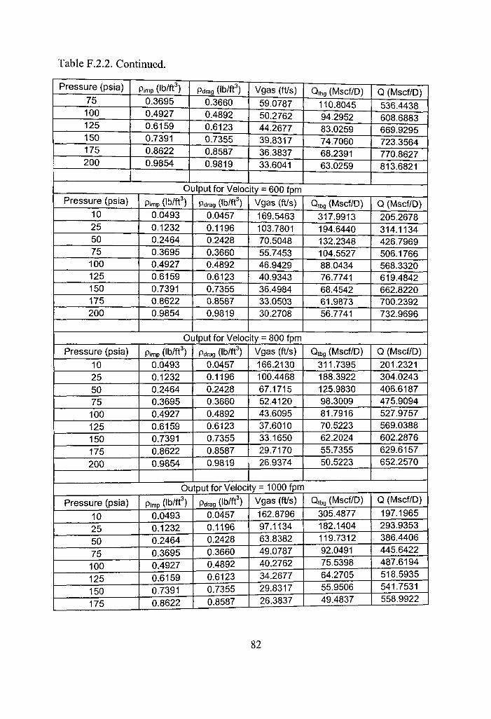
Table F.2.2. Continued.
Pressure (psia)
75 100 125 150 175 200
Pimp (lb/ft')
0.3695 0.4927 0.6159 0.7391 0.8622 0.9854
Pdrag (lb/ft')
0.3660 0.4892 0.6123 0.7355 0.8587 0.9819
Vgas (ft/s)
59.0787 50.2762 44.2677 39.8317 36.3837 33.6041
Q,bg (Mscf/D)
110.8045 94.2952 83.0259 74.7060 68.2391 63.0259
Q (Mscf/D) 536.4438 608.6883 669.9295 723.3564 770.8627 813.6821
Output for Velocity = 600 fpm Pressure (psia)
10 25 50 75 100 125 150 175 200
Pimp (lb/ft')
0.0493 0.1232 0.2464 0.3695 0.4927 0.6159 0.7391 0.8622 0.9854
Pdrag (lb/ft') 0.0457 0.1196 0.2428 0.3660 0.4892 0.6123 0.7355 0.8587 0.9819
Vgas (ft/s)
169.5463 103.7801 70.5048 55.7453 46.9429 40.9343 36.4984 33.0503 30.2708
Qtbg (Mscf/D)
317.9913 194.6440 132.2348 104.5527 88.0434 76.7741 68.4542 61.9873 56.7741
Q (Mscf/D) 205.2678 314.1134 426.7969 506.1766 568.3320 619.4842 662.8220 700.2392 732.9696
Output for Velocity = 800 fpm Pressure (psia)
10 25 50 75 100 125 150 175 200
Pimp (lb/ft') 0.0493 0.1232 0.2464 0.3695 0.4927 0.6159 0.7391 0.8622 0.9854
Pdrag (lb/ft') 0.0457 0.1196 0.2428 0.3660 0.4892 0.6123 0.7355 0.8587 0.9819
Vgas (ft/s) 166.2130 100.4468 67.1715 52.4120 43.6095 37.6010 33.1650 29.7170 26.9374
Qtbg (Mscf/D)
311.7395 188.3922 125.9830 98.3009 81.7916 70.5223 62.2024 55.7355 50.5223
Q (Mscf/D) 201.2321 304.0243 406.6187 475.9094 527.9757 569.0388 602.2876 629.6157 652.2570
Output for Velocity = 1000 fpm
Pressure (psia)
10 25 50 75 100 125 150 175
Pimp (Ib/ft^) 0.0493 0.1232 0.2464 0.3695 0.4927 0.6159 0.7391 0.8622
Pdrag (lb/ft') 0.0457 0.1196 0.2428 0.3660 0.4892 0.6123 0.7355 0.8587
Vgas (ft/s) 162.8796 97.1134 63.8382 49.0787 40.2762 34.2677 29.8317 26.3837
Qtbg (Mscf/D)
305.4877 182.1404 119.7312 92.0491 75.5398 64.2705 55.9506 49.4837
Q (Mscf/D)
197.1965 293.9353 386.4406 445.6422 487.6194 518.5935 541.7531 558.9922
82

Table F.2.2. Continued.
Pressure (psia)
200
Pimp
(Ib/ft^) 0.9854
Pdrag (lb/ft')
0.9819
Vgas (ft/s)
23.6041
Qtbg (Mscf/D)
44.2705
Q (Mscf/D)
571.5444
Output for Velocity = 1200 fpm Pressure (psia)
10 25 50 75 100 125 150 175 200
Pimp (lb/ft')
0.0493 0.1232 0.2464 0.3695 0.4927 0.6159 0.7391 0.8622 0.9854
Pdrag (lb/ft')
0.0457 0.1196 0.2428 0.3660 0.4892 0.6123 0.7355 0.8587 0.9819
Vgas (ft/s) 159.5463 93.7801 60.5048 45.7453 36.9429 30.9343 26.4984 23.0503 20.2708
Q,bg (Mscf/D)
299.2359 175.8886 113.4794 85.7973 69.2879 58.0187 49.6988 43.2319 38.0187
Q (Mscf/D) 193.1609 283.8462 366.2625 415.3750 447.2632 468.1481 481.2187 488.3687 490.8319
Output for Velocity = 1400 fpm Pressure (psia)
10 25 50 75 100 125 150 175 200
Pimp (Ib/ft^) J
0.0493 0.1232 0.2464 0.3695 0.4927 0.6159 0.7391 0.8622 0.9854
Pdrag (lb/ft')
0.0457 0.1196 0.2428 0.3660 0.4892 0.6123 0.7355 0.8587 0.9819
Vgas (ft/s)
156.2130 90.4468 57.1715 42.4120 33.6095 27.6010 23.1650 19.7170 16.9374
Q,bg (Mscf/D)
292.9841 169.6368 107.2276 79.5455 63.0361 51.7669 43.4470 36.9801 31.7669
Q (Mscf/D)
189.1252 273.7571 346.0843 385.1077 406.9069 417.7028 420.6843 417.7452 410.1193
Output for Velocity = 1600 fpm
Pressure (psia)
10 25 50 75 100 125 150 175 200
Pimp (lb/ft')
0.0493 0.1232 0.2464 0.3695 0.4927 0.6159 0.7391 0.8622 0.9854
Pdrag (Ib/ft^)
0.0457 0.1196 0.2428 0.3660 0.4892 0.6123 0.7355 0.8587 0.9819
Vgas (ft/s)
152.8796 87.1134 53.8382 39.0787 30.2762 24.2677 19.8317 16.3837 13.6041
Qtbg (Mscf/D)
286.7323 163.3849 100.9758 73.2937 56.7843 45.5151 37.1952 30.7283 25.5151
Q (Mscf/D)
185.0896 263.6680 325.9062 354.8405 366.5506 367.2574 360.1499 347.1218 329.4068
Oiitpiit for Velocity = 1800 fpm
Pressure (psia) Pimp (lb/ft') Pdraq (Ib/ft^) Vgas (ft/s) Qtbg (Mscf/D) Q (Mscf/D)
83
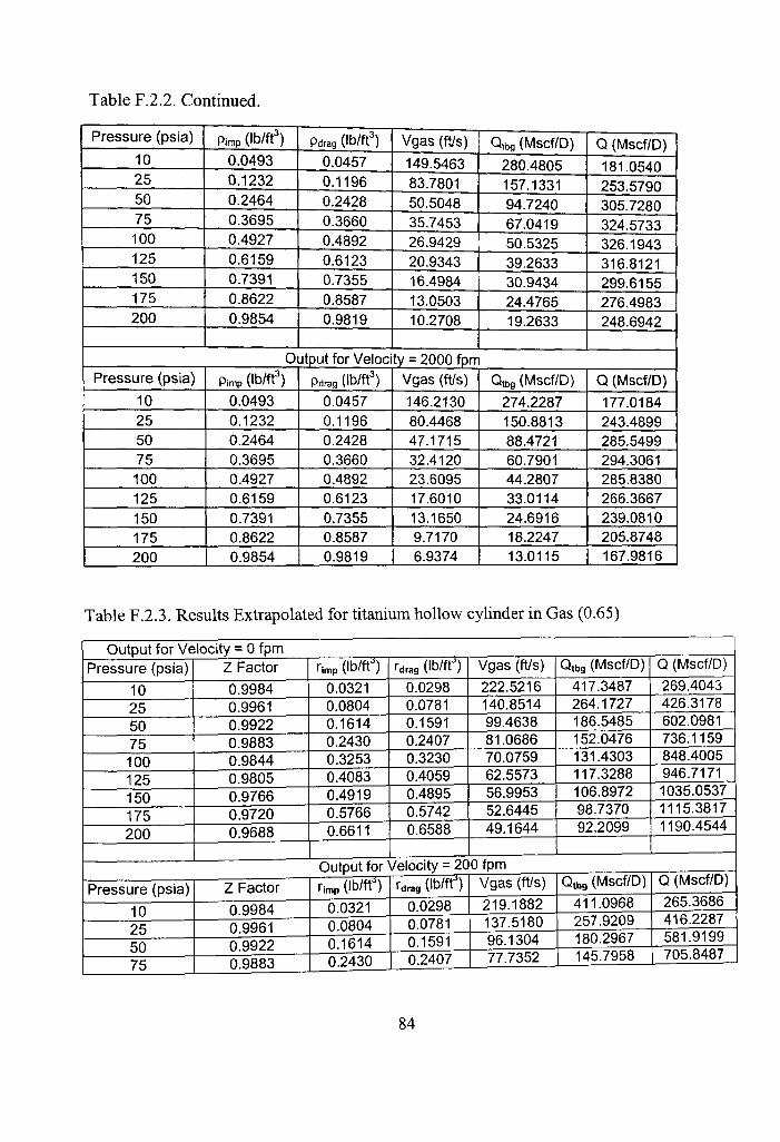
Table F.2.2. Continued.
Pressure (psia)
10 25 50 75 100 125 150 175 200
Pimp (lb/ft')
0.0493 0.1232 0.2464 0.3695 0.4927 0.6159 0.7391 0.8622 0.9854
Pdrag (ib/ft')
0.0457 0.1196 0.2428 0.3660 0.4892 0.6123 0.7355 0.8587 0.9819
Vgas (ft/s)
149.5463 83.7801 50.5048 35.7453 26.9429 20.9343 16.4984 13.0503 10.2708
Qtbg (Mscf/D)
280.4805 157.1331 94.7240 67.0419 50.5325 39.2633 30.9434 24.4765 19.2633
Q (Mscf/D)
181.0540 253.5790 305.7280 324.5733 326.1943 316.8121 299.6155 276.4983 248.6942
Output for Velocity = 2000 fpm Pressure (psia)
10 25 50 75 100 125 150 175 200
Pimp (lb/ft')
0.0493 0.1232 0.2464 0.3695 0.4927 0.6159 0.7391 0.8622 0.9854
Pdrag (lb/ft')
0.0457 0.1196 0.2428 0.3660 0.4892 0.6123 0.7355 0.8587 0.9819
Vgas (ft/s)
146.2130 80.4468 47.1715 32.4120 23.6095 17.6010 13.1650 9.7170 6.9374
Q,bg (Mscf/D)
274.2287 150.8813 88.4721 60.7901 44.2807 33.0114 24.6916 18.2247 13.0115
Q (Mscf/D)
177.0184 243.4899 285.5499 294.3061 285.8380 266.3667 239.0810 205.8748 167.9816
Table F.2.3. Results Extrapolated for titanium hollow cylinder in Gas (0.65)
Output for Velocity = 0 fpm Pressure (psia)
10 25 50 75 100 125 150 175 200
Z Factor
0.9984 0.9961 0.9922 0.9883 0.9844 0.9805 0.9766 0.9720 0.9688
rimp (Ib/ft^)
0.0321 0.0804 0.1614 0.2430 0.3253 0.4083 0.4919 0.5766 0.6611
rdrag (Ib/ft^)
0.0298 0.0781 0.1591 0.2407 0.3230 0.4059 0.4895 0.5742 0.6588
Vgas (ft/s)
222.5216 140.8514 99.4638 81.0686 70.0759 62.5573 56.9953 52.6445 49.1644
Q,bg (Mscf/D)
417.3487 264.1727 186.5485 152.0476 131.4303 117.3288 106.8972 98.7370 92.2099
Q (Mscf/D)
269.4043 426.3178 602.0981 736.1159 848.4005 946.7171 1035.0537 1115.3817 1190.4544
Output for Velocity = 200 tpm
Pressure (psia)
10 25 50 75
Z Factor
0.9984 0.9961 0.9922 0.9883
Timp (Ib/ft^)
0.0321 0.0804 0.1614 0.2430
Tdrag (ib/ft1
0.0298 0.0781 0.1591 0.2407
Vgas (ft/s)
219.1882 137.5180 96.1304 77.7352
Q,bg (Mscf/D)
411.0968 257.9209 180.2967 145.7958
Q (Msct/U)
265.3686 416.2287 581.9199 705.8487
84

Table F.2.3. Continued.
Pressure (psia)
100 125 150 175 200
Z Factor
0.9844 0.9805 0.9766 0.9720 0.9688
rimp (Ib/ft- )
0.3253 0.4083 0.4919 0.5766 0.6611
Tdrag (lb/ft")
0.3230 0.4059 0.4895 0.5742 0.6588
Vgas (ft/s)
66.7425 59.2239 53.6620 49.3112 45.8310
Qtbg (Mscf/D)
125.1785 111.0770 100.6454 92.4852 85.9580
Q (Mscf/D)
808.0443 896.2717 974.5193 1044.7582 1109.7418
Output for Velocity = 400 fpm Pressure (psia)
10 25 50 75 100 125 150 175 200
Z Factor
0.9984 0.9961 0.9922 0.9883 0.9844 0.9805 0.9766 0.9720 0.9688
Hmp (Ib/fty
0.0321 0.0804 0.1614 0.2430 0.3253 0.4083 0.4919 0.5766 0.6611
Tdrag (Ib/ft^
0.0298 0.0781 0.1591 0.2407 0.3230 0.4059 0.4895 0.5742 0.6588
Vgas (ft/s)
215.8549 134.1847 92.7971 74.4019 63.4092 55.8906 50.3287 45.9778 42.4977
Qtbg (Mscf/D)
404.8450 251.6691 174.0449 139.5440 118.9267 104.8252 94.3935 86.2334 79.7062
Q (Mscf/D)
261.3330 406.1397 561.7418 675.5815 767.6880 845.8264 913.9849 974.1347 1029.0293
Output for Velocity = 600 fpm
Pressure (psia)
10 25 50 75 100 125 150 175 200
Z Factor
0.9984 0.9961 0.9922 0.9883 0.9844 0.9805 0.9766 0.9720 0.9688
Hmp (lb/ft')
0.0321 0.0804 0.1614 0.2430 0.3253 0.4083 0.4919 0.5766 0.6611
rdrag (Ib/ft )
0.0298 0.0781 0.1591 0.2407 0.3230 0.4059 0.4895 0.5742 0.6588
Vgas (ft/s)
212.5216 130.8514 89.4638 71.0686 60.0759 52.5573 46.9953 42.6445 39.1644
Q,bg (Mscf/D)
398.5932 245.4173 167.7931 133.2921 112.6749 98.5734 88.1417 79.9816 73.4544
Q (Mscf/D)
257.2974 396.0506 541.5637 645.3143 727.3317 795.3810 853.4504 903.5112 948.3167
Output for Velocity = 800 fpm
Pressure (psia)
10 25 50 75 100 125 150 175 200
Z Factor
0.9984 0.9961 0.9922 0.9883 0.9844 0.9805 0.9766 0.9720 0.9688
rimp (Ib/ft )
0.0321 0.0804 0.1614 0.2430 0.3253 0.4083 0.4919 0.5766 0.6611
rdrag {Mf) 0.0298 0.0781 0.1591 0.2407 0.3230 0.4059 0.4895 0.5742 0.6588
Vgas (ft/s)
209.1882 127.5180 86.1304 67.7352 56.7425 49.2239 43.6620 39.3112 35.8310
Q,bg (Mscf/D)
392.3414 239.1655 161.5413 127.0403 106.4231 92.3216 81.8899 73.7298 67.2026
Q (Mscf/D)
253.2618 385.9615 521.3855 615.0471 686.9754 744.9357 792.9160 832.8878 867.6042
85

Table F.2.3. Continued.
Pressure (psia) 10 25 50 75 100 125 150 175 200
Z Factor 0.9984 0.9961 0.9922 0.9883 0.9844 0.9805 0.9766 0.9720 0.9688
Output for Velocity = 1000 fpm rimp (lb/ft")
0.0321 0.0804 0.1614 0.2430 0.3253 0.4083 0.4919 0.5766 0.6611
rdrag (Ib/ff^)
0.0298 0.0781 0.1591 0.2407 0.3230 0.4059 0.4895 0.5742 0.6588
Vgas (ft/s)
205.8549 124.1847 82.7971 64.4019 534092 45.8906 40.3287 35.9778 324977
Output for Velocity = 1200 fpm Pressure (psia)
10 25 50 75 100 125 150 175 200
Pressure (psia)
10 25 50 75 100 125 150 175 200
Pressure (psia)
10 25 50 75 100 125 150 175
Z Factor 0.9984 0.9961 0.9922 0.9883 0.9844 0.9805 0.9766 0.9720 0.9688
Z Factor
0.9984 0.9961 0.9922 _j 0.9883 0.9844 0.9805 0.9766 0.9720 0.9688
Z Factor
0.9984 0.9961 0.9922 0.9883 0.9844 0.9805 0.9766 0.9720
Hmp (Ib/ftT 0.0321 0.0804 0.1614 0.2430 0.3253 0.4083 0.4919 0.5766 0.6611
rdrag (lb/ft ' )
0.0298 0.0781 0.1591 0.2407 0.3230 0.4059 0.4895 0.5742 0.6588
Output for Velocity = 14( rimp ( Ib / f f )
0.0321 0.0804 0.1614 0.2430 0.3253 0.4083 0.4919 0.5766 0.6611
rdrag (Ib/ft^)
0.0298 0.0781 0.1591 0.2407 0.3230 0.4059 0.4895 0.5742 0.6588
Output for Velocity = 16 rimp (Ib/ft^)
0.0321 0.0804 0.1614 0.2430 0.3253 0.4083 0.4919 0.5766
rdrag (Ib/ft^)
0.0298 0.0781 0.1591 0.2407 0.3230 0.4059 0.4895 0.5742
Vgas (ft/s) 202.5216 120.8514 79.4638 61.0686 50.0759 42.5573 36.9953 32.6445 29.1644
DO fpm Vgas (ft/s)
199.1882 117.5180 76.1304 57.7352 46.7425 39.2239 33.6620 29.3112 25.8310
DO fpm Vgas (ft/s)
195.8549 114.1847 72.7971 54.4019 43.4092 35.8906 30.3287 25.9778
Q.bg (Mscf/D)
386.0896 232.9137 155.2895 120.7885 100.1713 86.0698 75.6381 67.4780 60.9508
Qtbg (Mscf/D)
379.8378 226.6619 149.0377 114.5367 93.9194 79.8180 69.3863 61.2262 54.6990
Qtbg (Mscf/D)
373.5860 220.4101 142.7859 108.2849 87.6676 73.5662 63.1345 54.9744 48.4472
Q,bg (Mscf/D)
367.3342 214.1583 136.5340 102.0331 81.4158 67.3144 56.8827 48.7226
Q (Mscf/D)
249.2261 375.8725 501.2074 584.7799 646.6191 694.4903 732.3816 762.2643 786.8916
Q (Mscf/D) 245.1905 365.7834 481.0292 554.5126 606.2629 644.0450 671.8472 691.6408 706.1790
Q (Mscf/D)
241.1549 355.6943 460.8511 524.2454 565.9066 593.5996 611.3128 621.0173 625.4665
Q (Mscf/D)
237.1192 345.6052 440.6730 493.9782 525.5503 543.1543 550.7783 550.3938
86

Table F.2.3. Continued.
Pressure (psia)
10 25 50 75 100 125 150 175 200 J
Output for Velocity = 1800 fpm Z Factor
0.9984 0.9961 0.9922 0.9883 0.9844 0.9805 0.9766 0.9720 0.9688
Timp mn 0.0321 0.0804 0.1614 0.2430 0.3253 0.4083 0.4919 0.5766 0.6611
rdrag (IWft )
0.0298 0.0781 0.1591 0.2407 0.3230 0.4059 0.4895 0.5742 0.6588
Vgas (ft/s)
192.5216 110.8514 69.4638 51.0686 40.0759 32.5573 26.9953 22.6445 19.1644
Qtbg (Mscf/D)
361.0824 207.9065 130.2822 95.7813 75.1640 61.0626 50.6309 42.4707 35.9436
Q (Mscf/D)
233.0836 335.5162 420.4948 463.7110 485.1940 492.7089 490.2439 479.7703 464.0414
Output for Velocity = 2000 fpm Pressure (psia)
10 25 50 75 100 125 150 175 200
Z Factor
0.9984 0.9961 0.9922 0.9883 0.9844 0.9805 0.9766 0.9720 0.9688
rimp (Ib/ft1
0.0321 0.0804 0.1614 0.2430 0.3253 0.4083 0.4919 0.5766 0.6611
rdrag (Ib/ft
0.0298 0.0781 0.1591 0.2407 0.3230 0.4059 0.4895 0.5742 0.6588
Vgas (ft/s)
189.1882 107.5180 66.1304 47.7352 36.7425 29.2239 23.6620 19.3112 15.8310
Qtbg (Mscf/D)
354.8306 201.6547 124.0304 89.5295 68.9122 54.8107 44.3791 36.2189 29.6918
Q (Mscf/D)
229.0480 325.4271 400.3167 433.4438 444.8377 442.2636 429.7095 409.1468 383.3288
F.3 Data for Ball and Hollow Cylinder Combined
Table F.3.1. Physical parameters for the 2 in. titanium set
Parameter Clearance (Plunger-Tubing)
Cylinder Outer Diameter Weight
Pressure Drop (measured) Pressure Drop (calculated)
Value 0.145 1.85
2.3129 0.8 0.86
Units Inch Inch Lbs Psi Psi
87

Table F.3.2.1. Two in. titanium set for 500 fpm fall velocity
0.25 bbl of water and 64.33 ft Slug length) Pressure (psia)
23.7 50 100
250 500
750 1000
Z Factor
0.9962 0.995 0.9944
0.9572 0.9156 0.8761 0.8371
Pimp (lb/ft') 0.07746 0.16362
0.32744
0.85040 1.77809 2.78738 3.88965
Vgas (ft/s) 91.314 65.422
48.686 33.371 25.648 22.162 20.040
Qtbg (Mcf/D) 171.285 122.718
91.325 62.597 48.110 41.572 37.590
Q (Mscf/D) 266.419 402.696 599.358 1027.049 1578.724 2046.238 2467.032
0.5 bbl of water and 128.66 ft Slug lenqth Pressure (psia)
23.7 50
100
250
500
750
1000
Z Factor
0.9962 0.995
0.9944
0.9572
0.9156 0.8761
0.8371
Pimp (lb/ft') 0.07746 0.16362
0.32744
0.85040
1.77809 2.78738
3.88965
Vgas (ft/s) 167.276 117.689 85.633
56.297
41.503 34.826
30.760
Qtbg (Mcf/D) 313.774 220.760 160.630
105.602
77.851 65.325
57.699
Q (Mscf/D)
488.049 724.415 1054.201
1732.638
2554.653 3215.435 3786.713
0.75 bbl of water and 193.0 ft Slug length Pressure (psia)
23.7 50
100
250
500
750
1000
Z Factor 0.9962 0.995
0.9944
0.9572
0.9156
0.8761
0.8371
Pimp (lb/ft') 0.07746 0.16362
0.32744
0.85040
1.77809 2.78738
3.88965
Vgas (ft/s) 244.740 170.989
123.311
79.677 57.672 47.739
41.691
Qtbg (Mcf/D) 459.081 320.740
231.305
149.456 108.180
89.548 78.204
Q (Mscf/D) 714.060 1052.494
1518.035
2452.176 3549.876 4407.747 5132.484
1 bbl of water and 257.33 ft Slug length
Pressure (psia) 23.7 50 100 250 500
750
1000
Z Factor 0.9962 0.995
0.9944 0.9572 0.9156
0.8761
0.8371
Pimp (Ib/ft^) 0.07746 0.16362 0.32744 0.85040 1.77809
2.78738
3.88965
Vgas (ft/s) 322.598 224.560 161.180 103.175 73.922
60.718
52.679
Qtbg (Mcf/D)
605.124 421.227 302.338 193.534 138.662
113.895
98.814
Q (Mscf/D)
941.218 1382.238 1984.223 3175.365 4550.149
5606.109
6485.084
0.0 bbl of water
Pressure (psia)
23.7
50
Z Factor
0.9962
0.995
Pimp (lb/ft') 0.07746
0,16362
Vgas (ft/s) 35.8690
27.2730
Qtbg (Mcf/D)
67.2825
51.1582
Q (Mscf/D)
104.6520
167.8738
88

Table F.3.2.1 Continued.
Pressure (psia)
100 250 500 750
1000
Z Factor
0.9944 0.9572 0.9156 0.8761
0.8371
Pimp(lb/ft^)
0.32744 0.85040 1.77809 2.78738
3.88965
Vgas (ft/s)
21.7186 16.6374 14.0756 12.9194 12.2155
Q,bg (Mcf/D)
40.7395 31.2082 26.4028 24.2340 22.9136
Table F.3.2.2. Two in. titanium set for 1000 ^ m fall velocity
Q (Mscf/D)
267.3702 512.0417 866.3960 1192.8439 1503.8002
0.25 bbl of water and 64.33 ft Slug lenqth Pressure (psia)
23.7 50
100 250
500 750 1000
Z Factor
0.9962 0.995
0.9944 0.9572
0.9156 0.8761 0.8371
Pimp (lb/ft')
0.07746 0.16362
0.32744
0.85040 1.77809 2.78738 3.88965
Vgas (ft/s)
99.802 73.863 57.095
41.751 34.014 30.521 28.395
Qtbg (Mcf/D)
187.208 138.550 107.098
78.316 63.803 57.252 53.263
Q (Mscf/D) 291.185 454.647 702.876
1284.962 2093.661 2818.042 3495.615
0.5 bbl of water and 128.66 ft Slug length Pressure (psia)
23.7 50
100
250
500
750
1000
Z Factor
0.9962 0.995 0.9944
0.9572
0.9156
0.8761
0.8371
Pimp (lb/ft')
0.07746 0.16362 0.32744
0.85040
1.77809 2.78738
3.88965
Vgas (ft/s)
175.924 126.239
94.120
64.725
49.902
43.211
39.137
Qtbg (Mcf/D)
329.996 236.797 176.548
121.411
93.606 81.055
73.413
Q (Mscf/D) 513.279 777.041 1158.672
1992.030 3071.636
3989.689 4818.062
0.75 bbl of water and 193.0 ft Slug length
Pressure (psia) 23.7 50
100
250
500
750
1000
Z Factor 0.9962 0.995
0.9944
0.9572
0.9156
0.8761
0.8371
Pimp (lb/ft')
0.07746 0.16362
0.32744
0.85040
1.77809
2.78738
3.88965
Vgas (ft/s)
253.547 179.648
131.874
88.153
66.104
56.151
50.092
Qtbg (Mcf/D)
475.599 336.981
247.368
165.356
123.996
105.328
93.961
Q (Mscf/D)
739.753 1105.791
1623.455
2713.040
4068.894 5184.440
6166.585
1 bbl of water and 257.33 ft Slug length
Pressure (psia)
23.7 50
Z Factor
0.9962 0.995
Pimp (lb/ft')
0.07746 0.16362
Vgas (ft/s)
331.562 233.328
Qtbg (Mcf/D)
621.939 437.673
Q (Mscf/D)
967.372 1436.206
89

Table F.3.2.2 Continued.
Pressure (psia)
100 250 500
750
1000
Z Factor
0.9944
0.9572
0.9156
0.8761
0.8371
Pimp (lb/ft')
0.32744
0.85040
1.77809
2.78738
3.88965
Vgas (ft/s)
169.820
111.698
82.387
69.157
61.101
Q,bg (Mcf/D)
318.546 209.522
154.541
129.723
114.613
Q (Mscf/D)
2090.591
3437.699
5071.200
6385.238
7521.934
0.0 bbl of water
Pressure (psia)
23.7
50 100 250 500 750
1000
Z Factor
0.9962
0.995
0.9944
0.9572
0.9156
0.8761
0.8371
Pimp (lb/ft')
0.07746
0.16362
0.32744
0.85040 1.77809
2.78738
3.88965
Vgas (ft/s)
44.22086
35.61907
30.06099
24.97631 22.41278
21.25581
20.55141
Qtbg (Mcf/D)
82.9488593
66.8137479
56.3879814
46.8502076 42.0415681
39.8713528
38.5500381
Q (Mscf/D)
129.01969
219.24671
370.06992
768.68565 1379.5777
1962.5443
2530.0089
90

PERMISSION TO COPY
In presenting this thesis in partial fulfillment of the requurements for a master's
degree at Texas Tech University or Texas Tech University Health Sciences Center, I
agree that the Library and my major department shall make it freely available for
research purposes. Permission to copy this thesis for scholarly purposes may be
granted by the Director of the Library or my major professor. It is understood that any
copying or publication of this thesis for financial gain shall not be allowed without my
further written permission and that any user may be liable for copyright infringement.
Agree (Permission is granted.)
Stiident Signature Date
Disagree (Permission is not granted.)
Student Signature Date