new (iterative) methods for solving the nuclear eigenvalue problem pisa 05
Post on 20-Dec-2015
220 views
TRANSCRIPT

New (iterative) methods for solving
the nuclear eigenvalue problem
Pisa 05

An importance sampling algorithm for large scale shell model calculations
F. AndreozziN. Lo IudiceA. Porrino.

Currently adopted methods
• Stochastic methodology: Monte Carlo (C.W. Johnson et al. PRL 92), suitable for ground state. Minus sign problem.
• Direct Diagonalization: Lanczos (see G.H. Golub and C.F. Van Loan Matrix Computations 96). Critical point: Sizes of the matrix.
• In between: Quantum MC (M. Honma et al. PRL 95). MC to select the relevant basis states. Problems: Redundancy, symmetries broken by the stochastic procedure.
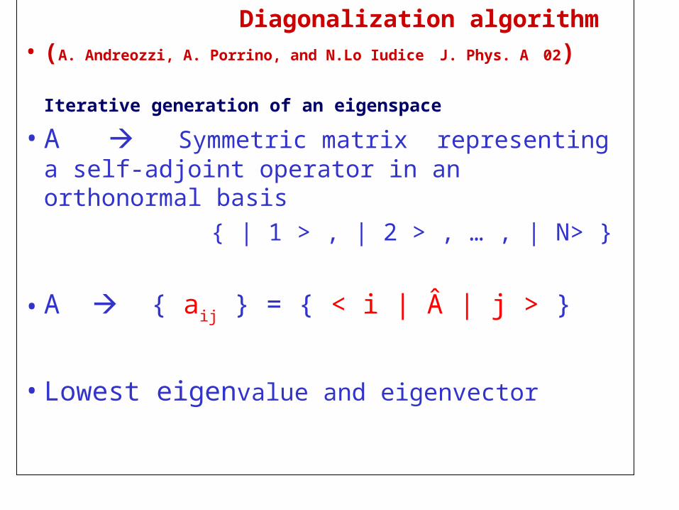
Diagonalization algorithm• (A. Andreozzi, A. Porrino, and N.Lo Iudice J. Phys. A 02)
Iterative generation of an eigenspace
• A Symmetric matrix representing a self-adjoint operator in an orthonormal basis
{ | 1 > , | 2 > , … , | N> }
• A { aij } = { < i | Â | j > }
• Lowest eigenvalue and eigenvector

a11 a12 a13 a14 …….. a1N
a21 a22 a23 a24 …….. a2N
a31 a32 a33 a34 …….. a3N
a41 a42 a43 a44 …….. a4N
………………………..
aN1 ………………….. aNN

λ1 = a11 | φ1 > = |1 >
basis { |1 >, |2 > }
Diagonalize the matrix
λ2 , | φ2 > = k1(2) |1 > + k2
(2) |2 >
a12
a22
a11
a21

Updated basis { | φ2 >, | 3 > }
Compute b3 = < φ2| Â | 3 >
= k1(2) a13 + k2
(2) a23
Diagonalize the matrix
λ3 , | φ3 > = Σ ki(3) | i >
i = 1, 3
b3
a33
λ2
b3
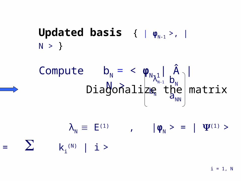
Updated basis { | φN-1 >, | N > }
Compute bN = < φN-1| Â | N >
Diagonalize the matrix
λN E(1) , |φN > = | (1) > = ki
(N) | i >
i = 1, N
End first iteration loop
bN
aNN
λN-1
bN

Compute b1 = < φ1(2)
| Â | 1 >
the states { | φ1(2)
>, |1> } are not linearly independent
Generalized eigenvalue problem
det ( - λ ) = 0
First step of the second iteration
Def. |φ 1(2) > = | ψ(1) > λ1
(2) = E(1)
b1
a11
λ1(2)
b1
< φ1(2)
|1 >
1
1 < φ1
(2) |1 >

E(1) , (1) E(2) , (2) ……
THEOREM
If the sequence E(i) converges , then
E(i) E (eigenvalue of the matrix A)
(i) (eigenvector of the matrix A)

Simultaneous determination of v eigensolutions
The structure of the algorithm unchanged
bj
ajj
λj-1
bj à BhT
Bh Λh
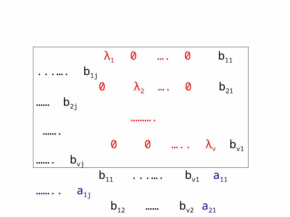
λ1 0 …. 0 b11 ...…. b1j
0 λ2 …. 0 b21 …… b2j
………. ……. 0 0 ….. λv bv1 ……. bvj
b11 ...…. bv1 a11 …….. a1j
b12 …… bv2 a21 …….. a2j
……. ……
b1j ……. bvj aj1 ..….. ajj

c• Easy implementation
• Variational foundation
• Robust Convergence to the extremal eigenvalues
Numerically stable and ghost-free solutions
Orthogonality of the computed eigenvectors
• Fast : O( N2) operations

IMPORTANCE SAMPLING
| Ψ > = Σ ci | i >
i = 1,N
localization property only m ( « N ) ci important
•diagonalization algorithm gives quite accurate solutions already in the first
approximation loop
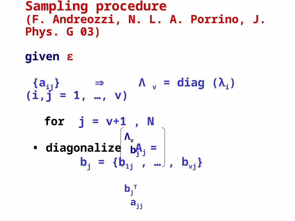
Sampling procedure (F. Andreozzi, N. L. A. Porrino, J. Phys. G 03)
given ε
{aij} Λ v = diag (λi) (i,j = 1, …, v) for j = v+1 , N
• diagonalize Aj = bj = {b1j , … , bvj} Λv bj
bjT ajj

• select the v lowest eigenvalues
λ1’ , … , λv’
• if Σ i = 1,v | λi’ - λi | > ε accept the j –th state
end loop
requires N ( v + 1)3 operations

Importance sampling reduces by a factor
N / Nsampled the number of operations
• The effectiveness of the reduction depends on the
localization properties of the wave function
• Increase of the localization through the use of a
correlated basis model space partitioning

Numerical Applications • Semimagic nuclei: 108Sn
• N=Z 48Cr
• N> Z 133Xe

108Sn
1h11/2
3s1/2
2d3/2
1g7/2
2d5/2
Realistic effective interaction deduced from Bonn A potential . Jπ = 2+ N = 17467


scaling with n (number of sampled states)
λ (n) = a + b (N/n) exp(-c N/n)
ε (n) = (d/n2) exp(-c N/n)
• it allows for high precision extrapolation n N

Heuristic argument
• consistency
ε(n) dλ / dn
• from the sampling condition (one target state)
Δλ = Σj Δλj = Σj bj2 / ( ajj - λ)

In the convergence region
• ajj - ann - n
• bj2 = <j-1 |H| j>2 (j-1 = i ci |i>)
small and random for j < n zero for j> n
bj2 exp (- j/n)

• Δλ b (N/n) exp(-c N/n)
• ε(n) dλ / dn (d/n2) exp(-c N/n)

Conclusions
• The algorithm is simple, robust and has a variational foundation
• Once endowed with the importance sampling, a) it keeps the extent of space truncation under strict
control b) it allows for extrapolation to exact eigensolutions• It is very promising for heavy nuclei• It may be applied to systems others than nuclei
(molecules, metal clusters, quantum dots etc.)

Nuclear Eigenvalue problem in a microscopic multiphonon space
Iterative equation of motion method
Naples(Andreozzi, Lo Iudice, Porrino)
Prague (Knapp, Kvasil)
collaboration

Preliminary remarks
• Standard Shell model is exact and complete within a given model space.
• Often the model space is spanned by ΔN = 0 –ħω Thus it does not include the high-energy configurations building up the
collective states.• TDA or RPA act in a more restricted but more selective space (p-h or
2qp configurations up to n ħω) and therefore are in general more suitable for collective excitations. They, however, do not account for anharmonic effects.
• A multiphonon space is needed for describing anharmonicity• Problem with multiphonon space: Antisymmetry Redundancy
Proposed way out: Equation of motion method

Eigenvalue problem: Formulation
Goal: Solving
H | α > = Eα | α >in a multiphonon space spanned by
| 0 >, |1, {ν1} >, |2, {ν2} >, ……. |n, {νn }>… where
|n, {νn }> = | ν1 ν2 …..νn >
| νi > = Σph C ph(νi ) B
+ph |0>
= Σph Cph(νi ) a+
p ah |0>

< n; νn | [H, B+ph] | n-1; νn-1 > =
Σν ’ < n; νn | H | n; ν’ > < n; ν’ | B+ph | n-1; νn-1 > -
Σν ’ < n; νn | B+
ph | n-1; ν’ > < n-1; ν’ | H | n-1; νn-1 >
< n; νn | H | n; ν’ > = Eνn δνnν’
< n-1; ν’ | H | n-1; νn-1 > = Eνn-1 δνn-1ν’
< n; νn | [H, B+ph] | n-1; νn-1 > =
(Eνn - Eνn-1
) < n; νn | B+
ph| n-1; νn-1 >.
Amplitude

The commutator yields:
< n; νn | [H, B+ph] | n-1; νn-1 > =
(εp- εh) < n; νn | B+
ph | n-1; νn-1 > +
+ [Σp’h’
Gp’ h h’ p < n; νn | B+
ph’| n-1; νn-1 >
+ Σ Gp’p’’p’’’p < n; νn | B+
p’h B+
p’’p’’’ | n-1; νn-1 >
+ Σ Gp’h’h’’p < n; νn | B+
p’h B+
h’h’’) | n-1; νn-1 >
+ Σ Gp’h p’’h’ < n; νn | B+
ph’ B+
p’p’’ | n-1; νn-1 > )
+ Σ Ghh’h’’h’’’ < n; νn | B+
ph’ B+
h’’h’’’) | n-1; νn-1 > ]
2
1
Amplitudes

Linearization
< n; νn | B+
p’h’ B+
p’’p’’’ | n-1; νn-1 >
< n; νn | B+
p’h’ B+
h’’h’’’) | n-1; νn-1 >
Î = Σ ν’ |n-1; ν’ >< n-1; ν’|
Î = Σ ν’ |n-1; ν’ >< n-1; ν’|
< n; νn | B+
p’h’ | n-1; ν’> ∙
· < n-1; ν’|B+p’’p’’’ | n-1; νn-1 >
< n; νn | B+
p’h’ | n-1; ν’> ∙
· < n-1; ν’|B+h’’h’’’ | n-1; νn-1 >
Amplitudes

Eigenvalue Equation М(n) X (n) = Eνn
X (n)
Where
X(n)νn-1
ph = < n; {νn} | B+
ph| n-1; {νn-1} >
(М(n))ph,p’h’(νn-1ν’n-1) = A ph,p’h’δνn-1ν’n-1
+ Hpp’(νn-1ν’n-1)δhh’
- Hhh’(νn-1ν’n-1)δpp’
Aph,p’h’ = (ep – eh + Eνn-1) δph,p’h’ - Gphp’h’
Hpp’(νn-1ν’n-1) = Σh1h2 Gph1p’h2
R h1h2 (νn-1ν’n-1)
- ½ Σp1p2 Gp’p1p2p
R p1p2 (νn-1ν’n-1)
Hhh’(νn-1ν’n-1) = Σp1p2 Ghp1h’p2
R p1p2 (νn-1ν’n-1)
- ½ Σh1h2 Gh’h1h2h
R h1h2 (νn-1ν’n-1)
Rab(ν’n-1νn-1) = < n-1; {ν’n-1} | B+ab| n-1; {νn-1} >

Redundancy• The states
B+ph| n-1; {νn-1} >
form an overcomplete linearlydependent set.
Is there a way out? Yes

• Let us perform the expansion in the redundant basis
|n; {νn}> = Σ νn-1ph Cph (νn νn-1) B+
ph| n-1;{νn-1} >
We obtain
X (n)νn-1
ph = < n; {νn} | B+
ph| n-1; {νn-1} > = Σ ν’n-1p’h’ Cp’h’(νn ν’n-1) Dphp’h’(νn-1 ν’n-1)
where
Dp’h’ph (νn-1 ν’n-1) =
< n-1; {ν’n-1} | B p’h’ B
+ph| n-1; {νn-1} >

In matrix form
X = D C
Therefore М X = E X
(МD)C = H C = E DCThis Eq. is ill defined with respect to
inversion (D is singular)

The way out: Choleski method• Choleski selects a basis of linear independent states
B+ph| n-1; {νn-1} >
spanning the physical subspace of the right dimension Ng < N
Using this basis, we compute a non singular matrix Ď and get (Ď-1МD)C = EC

Eq.
(Ď-1МD)C = E Cyields Ng exact eigensolutions for the
n-phonon subspace.
We can now move to the (n+1)-phonon subspace.
We only need to know X(n) and R(n).
X(n) is given by
X= D C

R(n) is given by the recursive relations
Rpp’(ν’nνn) = < n; {ν’n} | B+pp’| n; {νn} >
=Σ ν’n-1h Cp’h (νn ν’n-1) X(ν’n)
ν’n-1
ph +
Σ νn-1ν’n-1p1h Cph (νn νn-1) X(ν’n)
ν’n-1
p1h
Rpp’(ν’n-1νn-1)
Rhh’(ν’nνn) =
Σ ν’n-1p Cph’ (νn ν’n-1) X(ν’n)
ν’n-1
ph’ +
Σ νn-1ν’n-1ph1 Cph1 (νn νn-1) X
(ν’n)ν’n-1
ph1
Rhh’(ν’n-1νn-1)

Outcome of iteration: the Hamiltonian matrix
Eν0 { H ν0 ν1
} { H ν0 ν2 } { 0 } {0}
Eν1 0 ………. . .0 { H ν1 ν2
} {H ν1 ν3 } {0}
Eν’10……….0 { H ν’1 ν2
} {H ν’1 ν3 } {0}
E ν’’1 0….0
{ H ν’’1 ν2
} {H ν’’1 ν3} {0}
…………………………………..
Eν2 0……….. 0 {H ν2 ν3
} {H ν2 ν4}
Eν’2 0........ 0 {H ν’2 ν3
}{H ν’2 ν4}
Eν’’2 0..0 {H ν’’2 ν3
}{H ν’2 ν4}
……........................
Eν3 0 ..0 {H ν3 ν4
}
……………

The off diagonal termsare also computed by iteration
< n-1; {νn-1} | H| n; {νn} > = Σ (ph)k C(νn)
(ph)k
[< n-1; {νn-1} | [H, B+(ph)k
] | n-1; {νn-1}k > + Σ l X(ph)l
(νn-1 νn-2) < n-2; {νn-1}l | H| n-1; {νn}k > ]
< n-2; {νn-2} | H| n; {νn} > = Σ (ph)k C(νn)
(ph)k
[< n-2; {νn-2} | [H, B+(ph)k
] | n-1; {νn-1}k > +
X(ph)l (νn-2 νn-3) < n-3; {νn-3}l | H| n-1; {νn-1}k > ]

The Hamiltonian matrix
Eν0 { H ν0 ν1
} { H ν0 ν2 } { 0 } {0}
Eν1 0 ………. . .0 { H ν1 ν2
} {H ν1 ν3 } {0}
Eν’10……….0 { H ν’1 ν2
} {H ν’1 ν3 } {0}
E ν’’1 0….0
{ H ν’’1 ν2
} {H ν’’1 ν3} {0}
…………………………………..
Eν2 0……….. 0 {H ν2 ν3
} {H ν2 ν4}
Eν’2 0........ 0 {H ν’2 ν3
}{H ν’2 ν4}
Eν’’2 0..0 {H ν’’2 ν3
}{H ν’2 ν4}
……........................
Eν3 0 ..0 {H ν3 ν4
}
……………

Properties of H
• It is composed of central diagonal blocks
• Each block corresponds to a given n-phonon subspace
• A given n-block is coupled only to (n1)- and (n2)-blocks
Partitioning Importance sampling
Severe truncation

Status of art: Program tests successfully completed
A = 16
Phonon space
p-configurations {d}
h-configurations {s p}-1
Hamiltonian : BonnA

Choleski effect Jπ = 0+ T = 1
Two-phonon space
122 26
Three phonon space
3142 329

Choleski effect Jπ = 3- T = 1
Two-phonon space
252 62
Three phonon space
14956 1438

Future program
Immediate applications• Coupled scheme p-h. Detailed study of • anharmonic effects on giant resonances• Peculiar collective modes: i. ISGDR (squeezed mode), which requires up to
3ħω p-h configurationsii. Twist mode (orbital M2 mode)iii. Double GDR

Future program
• In parallel
Eq. of M. in uncoupled (spherical and deformed) scheme
• From p-h to qp to treat open shell nuclei as a cheap alternative to large scale shell model

More ambitious goal
• Combine SM (iterative algorithm) with Eq. of M. to enlarge the SM space and study i.e. intruders
• It si possible since the Eq. of M. formalism holds for any vacuum state.
• It can actually be used as alternative to SM in several cases (closed subshells)


• In many cases the information of interest is restricted to a few (usually low-lying) states whose accurate description presumably requires only a limited subset of the basis states
• Identification of the relevant components implies the knowledge of the wave function
Adaptive diagonalization algorithm


Bh = { <φi(h-1) | Â | j > } i = 1, …, v
j = 1, …, p
à is a principal submatrix of A:
an+p,n+p….an+p,n+2an+p,n+1
….….….….
an+2,n+p….an+2,n+2an+2,n+1
an+1,n+p….an+1,n+2an+1,n+1
à =


• a more efficient way through the similarity transform A’ = Ω -1 A Ω
Ω =
ω v-dimensional row vector
Iv 0
ω 1


transformed matrix A’ =
wj = - (ω · bj) ω - ω Λv + ajj ω + bjT
• decoupling condition
wj = 0 ajj - ω · bj eigenvalue of A
Λv+bj ω bj wj ajj - ω ·bj


Decoupling condition can be recast in form of a dispersion relation
ω ·bj = - Σi=1,v bij2 / (ajj-λi - ω ·bj)
(ω ·bj)min λ’max
interlacing property of the eigenvalues
Σ i = 1,v | λi’ - λi | = (ω ·bj)min > ε

• Choleski decomposition
Any real non singular symmetric matrix can be written as
D = L LT
Where L {lij} is a lower triangular matrix
and LT its transpose
Det{D} = (Det{L})2 = l112 l22
2 ...lii2…..

The elements of L are recursively defined as
l211 = d11
l11 lj1 = dj1 j=2,….,n
l2ii = dii – Σk=1,i-1 l
2ik
lii lji = dji – Σk=1,i-1 lik ljk

The decomposition goes on until
lrr = 0
Det{L} =0 Det{D} =0
| λr > is linearly dependent and is to be discarded

• Ordering
A linearly independent basis may yield an overlap matrix ill defined with respect to inversion.
To avoid this we arrange the basis in decreasing order
λii ≥ λjj j > I
This is automatically achieved
if we choose at each step
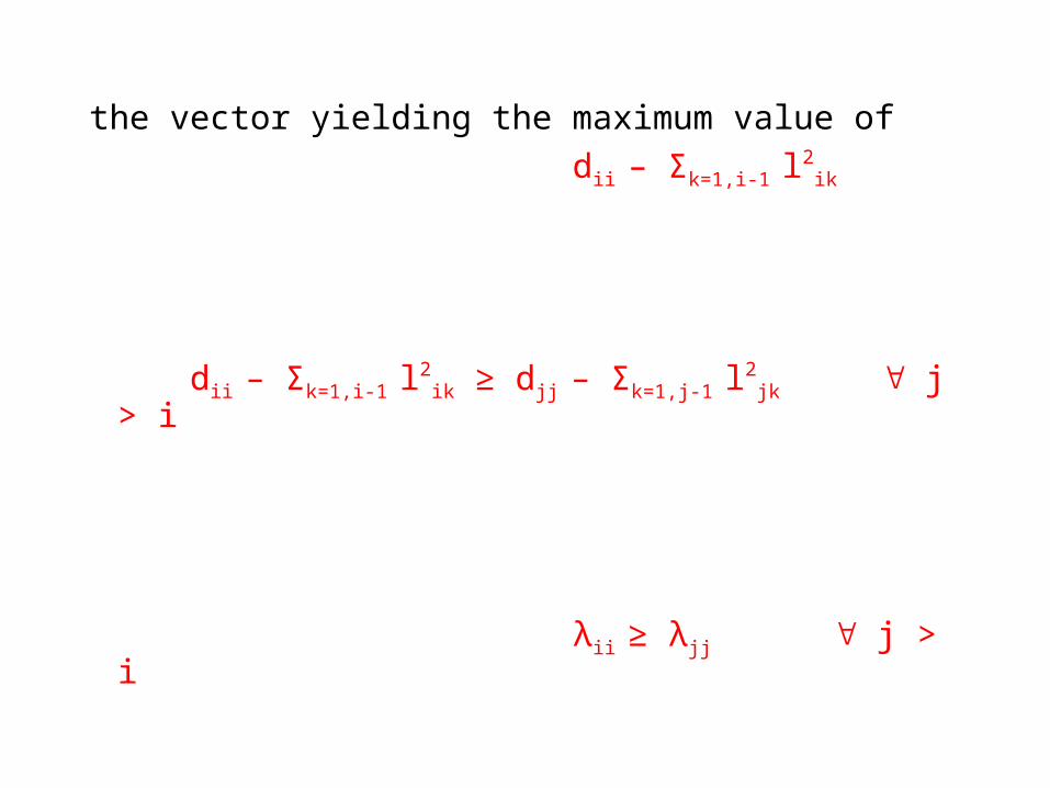
the vector yielding the maximum value of
dii – Σk=1,i-1 l2
ik
dii – Σk=1,i-1 l2
ik ≥ djj – Σk=1,j-1 l2
jk j > i
λii ≥ λjj j > i


• decompose accordingly the Hamiltonian
H = H1 + H2 + H12
solve the eigenvalue equations
Hi |αi Ni> = Eαi |αi Ni >
replace the standard shell model basis with
| α N > = | α1 N1 α2 N2 >
Orthonormal correlated basis