ii

c© 2015

Krzysztof Findeisen

All Rights Reserved

iii

Acknowledgments

This thesis would not have been possible without the help of many, many people both inside and

outside Caltech. First and foremost, I would like to thank my advisor, Lynne Hillenbrand, for her

guidance and support. Her mentorship made me the scientist I am today, and it was from her that I

learned the valuable skills of on-site observing, photometric and spectroscopic analysis, and technical

writing, among many others.

I must also thank the members of the PTF collaboration, whose tireless efforts over many years

made our North America Nebula survey possible. I owe a special thanks to Eran Ofek, David Levitan,

Branimir Sesar, and Russ Laher, who developed PTF’s photometric data reduction pipelines and

who patiently listened to both my questions and my bug reports. I am also grateful to the staff of

the Palomar, Keck, and Kitt Peak observatories, for their dedication to the facilities and for their

timely assistance whenever things went wrong.

I would like to thank the members of my thesis committee, John Carpenter, Lynne Hillenbrand,

John Johnson, Sterl Phinney, and Charles Steidel, for their valuable feedback throughout the last

three years. I also need to thank Cahill’s system administrators, Patrick Shopbell, Anu Mahabal,

and Jose Calderon, for helping me set up a database to manage the enormous amounts of data

this thesis required, and for always being patient with my requests for more and more disk space.

Many thanks also to the Cahill administrative staff for keeping everything running smoothly, and

for helping me with questions about paperwork or procedures.

The YSOVAR collaboration was a great source for feedback and ideas on this research, and

nearly everything I present here was vetted at YSOVAR group meetings in one form or another. I’d

like to especially thank Luisa Rebull. Not only did her prior research on the North America Nebula

form the foundation for my own work, she also volunteered her unpublished Spitzer photometry,

created valuable data products such as spectral energy distributions, and fielded an endless stream

of questions about the details of the data or their proper handling. She was amazingly helpful, and

really deserves credit for anything in this thesis involving infrared data (any errors in those sections

are, of course, entirely my own).

Additional advice and feedback came from the Time Domain Forum, where both Lynne Hil-

lenbrand and I presented preliminary versions of this work, and from private conversations with

iv

Nairn Baliber, Kirk Borne, John Carpenter, Ann Marie Cody, Kevin Covey, Ashish Mahabal, Adam

Miller, Timothy Morton, Chad Schafer, Keivan Stassun, Matthew Stevenson, and Neal Turner.

Many thanks also to Evan Kirby for his help in troubleshooting the DEIMOS pipeline software, and

to Eric Black for teaching me the art of scientific record-keeping.

Graduate school is a very different experience from college, and I was lucky to have two fantastic

mentors to help smooth the way. Mansi Kasliwal and Varun Bhalerao, thank you both for everything.

You helped make grad school not only survivable, but fun. I’d also like to thank Varun for inspiring

me to continue stargazing alongside my professional research, and for the herculean efforts he went

through to save the (former) Robinson/Downs Rooftop Observatory from destruction. I’d like to

thank Shriharsh Tendulkar and Mislav Balokovic for being my Cahill Rooftop Observatory co-

directors, Shriharsh, Scott Barenfeld, and Michael Eastwood for teaching me the way of the pundit,

Jose Calderon for being patient with a softball rookie, and everyone else who made the last seven

years as enjoyable as they were.

Last, but not least, a big thank you to my parents, Piotr and Joanna Findeisen, for their support

all along the path to becoming an astronomer. In many ways, I am here thanks to their love and

encouragement.

v

Abstract

Nearly all young stars are variable, with the variability traditionally divided into two classes: periodic

variables and aperiodic or “irregular” variables. Periodic variables have been studied extensively,

typically using periodograms, while aperiodic variables have received much less attention due to a

lack of standard statistical tools. However, aperiodic variability can serve as a powerful probe of

young star accretion physics and inner circumstellar disk structure. For my dissertation, I analyzed

data from a large-scale, long-term survey of the nearby North America Nebula complex, using

Palomar Transient Factory photometric time series collected on a nightly or every few night cadence

over several years. This survey is the most thorough exploration of variability in a sample of

thousands of young stars over time baselines of days to years, revealing a rich array of lightcurve

shapes, amplitudes, and timescales.

I have constrained the timescale distribution of all young variables, periodic and aperiodic, on

timescales from less than a day to ∼ 100 days. I have shown that the distribution of timescales for

aperiodic variables peaks at a few days, with relatively few (∼ 15%) sources dominated by variability

on tens of days or longer. My constraints on aperiodic timescale distributions are based on two new

tools, magnitude- vs. time-difference (∆m-∆t) plots and peak-finding plots, for describing aperiodic

lightcurves; this thesis provides simulations of their performance and presents recommendations on

how to apply them to aperiodic signals in other time series data sets. In addition, I have measured

the error introduced into colors or SEDs from combining photometry of variable sources taken at

different epochs. These are the first quantitative results to be presented on the distributions in

amplitude and time scale for young aperiodic variables, particularly those varying on timescales of

weeks to months.

vi

Contents

Acknowledgments iii

Abstract v

1 Introduction and Background 1

1.1 State of Knowledge of Young Stellar Physics . . . . . . . . . . . . . . . . . . . . . . . 2

1.1.1 Standard Model of Star Formation . . . . . . . . . . . . . . . . . . . . . . . . 2

1.1.2 Physics of Circumstellar Disks and Accretion . . . . . . . . . . . . . . . . . . 2

1.2 Current Knowledge and the Potential of Variability . . . . . . . . . . . . . . . . . . . 6

1.2.1 Major Variability Mechanisms . . . . . . . . . . . . . . . . . . . . . . . . . . 6

1.2.2 Previous Work on Periodic Variability . . . . . . . . . . . . . . . . . . . . . . 9

1.2.3 Previous Work on Aperiodic Variability . . . . . . . . . . . . . . . . . . . . . 10

1.3 Challenges for Variability Surveys . . . . . . . . . . . . . . . . . . . . . . . . . . . . . 11

1.4 Summary of Following Chapters . . . . . . . . . . . . . . . . . . . . . . . . . . . . . 12

1.5 References . . . . . . . . . . . . . . . . . . . . . . . . . . . . . . . . . . . . . . . . . . 14

2 Photometric and Supplementary Data 17

2.1 Introduction . . . . . . . . . . . . . . . . . . . . . . . . . . . . . . . . . . . . . . . . . 17

2.2 Overview of PTF . . . . . . . . . . . . . . . . . . . . . . . . . . . . . . . . . . . . . . 17

2.2.1 Instruments and Main Survey . . . . . . . . . . . . . . . . . . . . . . . . . . . 17

2.2.2 The PTF Photometric Pipeline . . . . . . . . . . . . . . . . . . . . . . . . . . 18

2.3 The PTF-NAN Survey . . . . . . . . . . . . . . . . . . . . . . . . . . . . . . . . . . . 19

2.3.1 The North America Nebula Complex . . . . . . . . . . . . . . . . . . . . . . . 19

2.3.2 Survey Overview . . . . . . . . . . . . . . . . . . . . . . . . . . . . . . . . . . 21

2.3.3 Cadence and Time Baselines . . . . . . . . . . . . . . . . . . . . . . . . . . . 21

2.3.4 Aliasing . . . . . . . . . . . . . . . . . . . . . . . . . . . . . . . . . . . . . . . 22

2.3.5 Systematics . . . . . . . . . . . . . . . . . . . . . . . . . . . . . . . . . . . . . 24

2.4 Supplementary Data . . . . . . . . . . . . . . . . . . . . . . . . . . . . . . . . . . . . 26

2.4.1 Spectroscopy . . . . . . . . . . . . . . . . . . . . . . . . . . . . . . . . . . . . 26

vii

2.4.2 Mid-IR Photometry . . . . . . . . . . . . . . . . . . . . . . . . . . . . . . . . 27

2.4.3 Near-IR Photometry . . . . . . . . . . . . . . . . . . . . . . . . . . . . . . . . 27

2.4.4 Hα Fluxes . . . . . . . . . . . . . . . . . . . . . . . . . . . . . . . . . . . . . . 28

2.5 Summary . . . . . . . . . . . . . . . . . . . . . . . . . . . . . . . . . . . . . . . . . . 28

2.6 References . . . . . . . . . . . . . . . . . . . . . . . . . . . . . . . . . . . . . . . . . . 30

3 Disk-Related Bursts and Fades in Young Stars 31

3.1 Introduction . . . . . . . . . . . . . . . . . . . . . . . . . . . . . . . . . . . . . . . . . 31

3.2 Photometric Data . . . . . . . . . . . . . . . . . . . . . . . . . . . . . . . . . . . . . 32

3.2.1 Identifying the Variables . . . . . . . . . . . . . . . . . . . . . . . . . . . . . . 32

3.3 Bursting and Fading Among Infrared Excess Sources . . . . . . . . . . . . . . . . . . 34

3.3.1 Sample Selection . . . . . . . . . . . . . . . . . . . . . . . . . . . . . . . . . . 34

3.3.2 Burster and Fader Statistics . . . . . . . . . . . . . . . . . . . . . . . . . . . . 38

3.3.3 Spectroscopic Characterization . . . . . . . . . . . . . . . . . . . . . . . . . . 38

3.4 The Burster Phenomenon . . . . . . . . . . . . . . . . . . . . . . . . . . . . . . . . . 42

3.4.1 Population Properties . . . . . . . . . . . . . . . . . . . . . . . . . . . . . . . 42

3.4.2 Constraints on Short-Term Accretion Outbursts . . . . . . . . . . . . . . . . 44

3.5 The Fader Phenomenon . . . . . . . . . . . . . . . . . . . . . . . . . . . . . . . . . . 46

3.6 Individual Sources of Interest . . . . . . . . . . . . . . . . . . . . . . . . . . . . . . . 48

3.6.1 FHO 26 . . . . . . . . . . . . . . . . . . . . . . . . . . . . . . . . . . . . . . . 48

3.6.2 [OSP2002] BRC 31 1 . . . . . . . . . . . . . . . . . . . . . . . . . . . . . . . . 48

3.6.3 FHO 18 . . . . . . . . . . . . . . . . . . . . . . . . . . . . . . . . . . . . . . . 51

3.6.4 FHO 27 . . . . . . . . . . . . . . . . . . . . . . . . . . . . . . . . . . . . . . . 52

3.6.5 FHO 28 . . . . . . . . . . . . . . . . . . . . . . . . . . . . . . . . . . . . . . . 53

3.7 Summary and Discussion . . . . . . . . . . . . . . . . . . . . . . . . . . . . . . . . . 55

3.7.1 Key Results . . . . . . . . . . . . . . . . . . . . . . . . . . . . . . . . . . . . . 55

3.7.2 Comparison to Previous Work . . . . . . . . . . . . . . . . . . . . . . . . . . 56

3.7.3 Limitations of the Present Work . . . . . . . . . . . . . . . . . . . . . . . . . 57

3.8 References . . . . . . . . . . . . . . . . . . . . . . . . . . . . . . . . . . . . . . . . . . 65

4 Theoretical Performance of Timescale Metrics 67

4.1 Introduction . . . . . . . . . . . . . . . . . . . . . . . . . . . . . . . . . . . . . . . . . 67

4.1.1 Motivation for an Analytic Treatment . . . . . . . . . . . . . . . . . . . . . . 68

4.1.2 Conventions in this Chapter . . . . . . . . . . . . . . . . . . . . . . . . . . . . 69

4.2 Test Signals . . . . . . . . . . . . . . . . . . . . . . . . . . . . . . . . . . . . . . . . . 72

4.2.1 Sinusoid . . . . . . . . . . . . . . . . . . . . . . . . . . . . . . . . . . . . . . . 72

4.2.2 AA Tau . . . . . . . . . . . . . . . . . . . . . . . . . . . . . . . . . . . . . . . 72

viii

4.2.3 White Noise . . . . . . . . . . . . . . . . . . . . . . . . . . . . . . . . . . . . . 73

4.2.4 Squared Exponential Gaussian Process . . . . . . . . . . . . . . . . . . . . . . 73

4.2.5 Two-Timescale Gaussian Process . . . . . . . . . . . . . . . . . . . . . . . . . 74

4.2.6 Damped Random Walk . . . . . . . . . . . . . . . . . . . . . . . . . . . . . . 74

4.2.7 Undamped Random Walk . . . . . . . . . . . . . . . . . . . . . . . . . . . . . 75

4.3 Overview of the Chapter . . . . . . . . . . . . . . . . . . . . . . . . . . . . . . . . . . 76

4.4 Structure Functions . . . . . . . . . . . . . . . . . . . . . . . . . . . . . . . . . . . . 77

4.4.1 Sinusoid . . . . . . . . . . . . . . . . . . . . . . . . . . . . . . . . . . . . . . . 78

4.4.2 AA Tau . . . . . . . . . . . . . . . . . . . . . . . . . . . . . . . . . . . . . . . 78

4.4.3 Gaussian Processes . . . . . . . . . . . . . . . . . . . . . . . . . . . . . . . . . 87

4.4.4 Summary . . . . . . . . . . . . . . . . . . . . . . . . . . . . . . . . . . . . . . 91

4.5 Autocovariance Functions . . . . . . . . . . . . . . . . . . . . . . . . . . . . . . . . . 92

4.5.1 Sinusoid . . . . . . . . . . . . . . . . . . . . . . . . . . . . . . . . . . . . . . . 94

4.5.2 AA Tau . . . . . . . . . . . . . . . . . . . . . . . . . . . . . . . . . . . . . . . 94


4.5.4 Summary . . . . . . . . . . . . . . . . . . . . . . . . . . . . . . . . . . . . . . 98

4.6 ∆m-∆t Plots . . . . . . . . . . . . . . . . . . . . . . . . . . . . . . . . . . . . . . . . 100

4.6.1 Sinusoid . . . . . . . . . . . . . . . . . . . . . . . . . . . . . . . . . . . . . . . 102

4.6.2 AA Tau . . . . . . . . . . . . . . . . . . . . . . . . . . . . . . . . . . . . . . . 104


4.6.4 Summary . . . . . . . . . . . . . . . . . . . . . . . . . . . . . . . . . . . . . . 118

4.7 Summary of Theoretical Results . . . . . . . . . . . . . . . . . . . . . . . . . . . . . 119

4.8 References . . . . . . . . . . . . . . . . . . . . . . . . . . . . . . . . . . . . . . . . . . 121

5 Numerical Performance of Timescale Metrics 122

5.1 Introduction . . . . . . . . . . . . . . . . . . . . . . . . . . . . . . . . . . . . . . . . . 122

5.1.1 LightcurveMC: an extensible lightcurve simulation program . . . . . . . . . . 123

5.1.2 Input Cadences . . . . . . . . . . . . . . . . . . . . . . . . . . . . . . . . . . . 123

5.2 Simulation Strategy . . . . . . . . . . . . . . . . . . . . . . . . . . . . . . . . . . . . 125

5.2.1 Simulations . . . . . . . . . . . . . . . . . . . . . . . . . . . . . . . . . . . . . 125

5.2.2 Timescale Characterization . . . . . . . . . . . . . . . . . . . . . . . . . . . . 126

5.3 Interpolated Autocorrelation Functions . . . . . . . . . . . . . . . . . . . . . . . . . . 127

5.3.1 Semi-Ideal ACFs as a Comparison Standard . . . . . . . . . . . . . . . . . . . 128

5.3.2 Example Results . . . . . . . . . . . . . . . . . . . . . . . . . . . . . . . . . . 128

5.3.3 Performance . . . . . . . . . . . . . . . . . . . . . . . . . . . . . . . . . . . . 130

5.3.4 Summary . . . . . . . . . . . . . . . . . . . . . . . . . . . . . . . . . . . . . . 135

ix

5.4 Scargle Autocorrelation Functions . . . . . . . . . . . . . . . . . . . . . . . . . . . . 137

5.5 ∆m-∆t Plots . . . . . . . . . . . . . . . . . . . . . . . . . . . . . . . . . . . . . . . . 137

5.5.1 Semi-Ideal ∆m-∆t Plots as a Comparison Standard . . . . . . . . . . . . . . 138

5.5.2 Example Results . . . . . . . . . . . . . . . . . . . . . . . . . . . . . . . . . . 139

5.5.3 Performance . . . . . . . . . . . . . . . . . . . . . . . . . . . . . . . . . . . . 139

5.5.4 Summary . . . . . . . . . . . . . . . . . . . . . . . . . . . . . . . . . . . . . . 145

5.6 Peak-Finding . . . . . . . . . . . . . . . . . . . . . . . . . . . . . . . . . . . . . . . . 147

5.6.1 Example Results . . . . . . . . . . . . . . . . . . . . . . . . . . . . . . . . . . 148

5.6.2 Performance . . . . . . . . . . . . . . . . . . . . . . . . . . . . . . . . . . . . 151

5.6.3 Summary . . . . . . . . . . . . . . . . . . . . . . . . . . . . . . . . . . . . . . 156

5.7 Gaussian Process Modeling . . . . . . . . . . . . . . . . . . . . . . . . . . . . . . . . 156

5.7.1 Performance . . . . . . . . . . . . . . . . . . . . . . . . . . . . . . . . . . . . 158

5.7.2 Summary . . . . . . . . . . . . . . . . . . . . . . . . . . . . . . . . . . . . . . 161

5.8 Revisiting Bursters and Faders . . . . . . . . . . . . . . . . . . . . . . . . . . . . . . 161

5.9 Summary of Numerical Results . . . . . . . . . . . . . . . . . . . . . . . . . . . . . . 167

5.10 References . . . . . . . . . . . . . . . . . . . . . . . . . . . . . . . . . . . . . . . . . . 169

6 Variability and Population Statistics in the North America Nebula 170

6.1 Introduction . . . . . . . . . . . . . . . . . . . . . . . . . . . . . . . . . . . . . . . . . 170

6.2 Previous Work in the North America Nebula . . . . . . . . . . . . . . . . . . . . . . 170

6.3 Source Statistics . . . . . . . . . . . . . . . . . . . . . . . . . . . . . . . . . . . . . . 171

6.4 Candidate Member Selection . . . . . . . . . . . . . . . . . . . . . . . . . . . . . . . 172

6.4.1 Identifying the Variables . . . . . . . . . . . . . . . . . . . . . . . . . . . . . . 172

6.4.2 Spectroscopic Candidates . . . . . . . . . . . . . . . . . . . . . . . . . . . . . 172

6.4.3 Revisiting Infrared Excess Assessment . . . . . . . . . . . . . . . . . . . . . . 173

6.4.4 Photometric Candidates . . . . . . . . . . . . . . . . . . . . . . . . . . . . . . 174

6.4.5 Variability as a Youth Indicator . . . . . . . . . . . . . . . . . . . . . . . . . . 177

6.4.6 New Candidate Members in the North America Nebula Complex . . . . . . . 179

6.5 Applying Timescale Metrics . . . . . . . . . . . . . . . . . . . . . . . . . . . . . . . . 181

6.5.1 Characterizing the Full Variability-Selected Sample of NAN Candidate Members181

6.5.2 Timescales in the North America Nebula Complex . . . . . . . . . . . . . . . 183

6.6 Variability Properties . . . . . . . . . . . . . . . . . . . . . . . . . . . . . . . . . . . 190

6.6.1 Timescales and Amplitudes . . . . . . . . . . . . . . . . . . . . . . . . . . . . 190

6.6.2 High-Amplitude Sources . . . . . . . . . . . . . . . . . . . . . . . . . . . . . . 192

6.6.3 Correlation with Infrared and Emission Line Properties . . . . . . . . . . . . 194

6.6.4 Evidence for Multiple Dominant Variability Mechanisms . . . . . . . . . . . . 199

x

6.7 Discussion . . . . . . . . . . . . . . . . . . . . . . . . . . . . . . . . . . . . . . . . . . 200

6.7.1 Comparison with Other State-of-the-Art Data Sets . . . . . . . . . . . . . . . 200

6.7.2 Systematic Errors in Non-Coeval Studies . . . . . . . . . . . . . . . . . . . . 202

6.8 Summary . . . . . . . . . . . . . . . . . . . . . . . . . . . . . . . . . . . . . . . . . . 205

6.9 References . . . . . . . . . . . . . . . . . . . . . . . . . . . . . . . . . . . . . . . . . . 206

7 The Promise of Aperiodic Variability 207

7.1 Review of Thesis Goals . . . . . . . . . . . . . . . . . . . . . . . . . . . . . . . . . . 207

7.2 New Techniques and Results . . . . . . . . . . . . . . . . . . . . . . . . . . . . . . . . 207

7.3 Publications . . . . . . . . . . . . . . . . . . . . . . . . . . . . . . . . . . . . . . . . . 210

7.4 Future Work . . . . . . . . . . . . . . . . . . . . . . . . . . . . . . . . . . . . . . . . 211

7.5 References . . . . . . . . . . . . . . . . . . . . . . . . . . . . . . . . . . . . . . . . . . 211

xi

List of Figures

1.1 Timescales and Amplitudes of Young Stellar Variability . . . . . . . . . . . . . . . . . 7

2.1 Map of North America Nebula Complex . . . . . . . . . . . . . . . . . . . . . . . . . . 20

2.2 PTF-NAN Observing Cadence . . . . . . . . . . . . . . . . . . . . . . . . . . . . . . . 21

2.3 PTF-NAN Window Function . . . . . . . . . . . . . . . . . . . . . . . . . . . . . . . . 23

2.4 Missing Sources Near a Filament . . . . . . . . . . . . . . . . . . . . . . . . . . . . . . 25

2.5 Spitzer Coverage of the North America Nebula Complex . . . . . . . . . . . . . . . . . 28

3.1 RMS vs. Magnitude for PTF Sources . . . . . . . . . . . . . . . . . . . . . . . . . . . 33

3.2 Color-Magnitude Diagrams for PTF Infrared Excess Sources . . . . . . . . . . . . . . 36

3.3 RMS Distribution of the PTF Sample . . . . . . . . . . . . . . . . . . . . . . . . . . . 37

3.4 Positions of Bursters and Faders in the North America Nebula Complex . . . . . . . . 39

3.5 Gallery of Bursters . . . . . . . . . . . . . . . . . . . . . . . . . . . . . . . . . . . . . . 40

3.6 Gallery of Faders . . . . . . . . . . . . . . . . . . . . . . . . . . . . . . . . . . . . . . . 41

3.7 Timescales and Amplitudes for Bursters and Faders . . . . . . . . . . . . . . . . . . . 43

3.8 Intermediate-Timescale Burst Profiles . . . . . . . . . . . . . . . . . . . . . . . . . . . 45

3.9 FHO 26 . . . . . . . . . . . . . . . . . . . . . . . . . . . . . . . . . . . . . . . . . . . . 49

3.10 BRC 31 1 . . . . . . . . . . . . . . . . . . . . . . . . . . . . . . . . . . . . . . . . . . . 50

3.11 FHO 18 . . . . . . . . . . . . . . . . . . . . . . . . . . . . . . . . . . . . . . . . . . . . 51

3.12 FHO 27 . . . . . . . . . . . . . . . . . . . . . . . . . . . . . . . . . . . . . . . . . . . . 52

3.13 FHO 28 . . . . . . . . . . . . . . . . . . . . . . . . . . . . . . . . . . . . . . . . . . . . 54

4.1 Gallery of Test Lightcurves . . . . . . . . . . . . . . . . . . . . . . . . . . . . . . . . . 70

4.2 Gallery of Test Lightcurves’ Power Spectra . . . . . . . . . . . . . . . . . . . . . . . . 71

4.3 Structure Functions for Sine and AA Tau . . . . . . . . . . . . . . . . . . . . . . . . . 79

4.4 Cases for AA Tau Structure Function Analysis . . . . . . . . . . . . . . . . . . . . . . 81

4.5 Structure Functions for White Noise and Squared Exponential Gaussian Process . . . 88

4.6 Structure Functions for Two-Timescale Gaussian Process . . . . . . . . . . . . . . . . 90

4.7 Structure Functions for Random Walks . . . . . . . . . . . . . . . . . . . . . . . . . . 91

4.8 Autocovariance Functions for Sine and AA Tau . . . . . . . . . . . . . . . . . . . . . . 95

xii

4.9 Autocovariance Functions for White Noise . . . . . . . . . . . . . . . . . . . . . . . . . 97

4.10 Autocovariance Functions for Squared Exponential Gaussian Process and Damped

Random Walk . . . . . . . . . . . . . . . . . . . . . . . . . . . . . . . . . . . . . . . . 98

4.11 Autocovariance Functions for Two-Timescale Gaussian Process . . . . . . . . . . . . . 99

4.12 ∆m-∆t Plot for Sinusoid . . . . . . . . . . . . . . . . . . . . . . . . . . . . . . . . . . 104

4.13 Cases for AA Tau ∆m-∆t Analysis . . . . . . . . . . . . . . . . . . . . . . . . . . . . . 109

4.14 ∆m-∆t Plot for AA Tau . . . . . . . . . . . . . . . . . . . . . . . . . . . . . . . . . . 112

4.15 ∆m-∆t Plot for White Noise . . . . . . . . . . . . . . . . . . . . . . . . . . . . . . . . 114

4.16 ∆m-∆t Plot for Squared Exponential Gaussian Process . . . . . . . . . . . . . . . . . 115

4.17 ∆m-∆t Plot for Two-Timescale Gaussian Process . . . . . . . . . . . . . . . . . . . . 116

4.18 ∆m-∆t Plot for Two-Timescale Gaussian Process . . . . . . . . . . . . . . . . . . . . 117

4.19 ∆m-∆t Plot for Damped Random Walk . . . . . . . . . . . . . . . . . . . . . . . . . . 118

4.20 ∆m-∆t Plot for Random Walk . . . . . . . . . . . . . . . . . . . . . . . . . . . . . . . 119

5.1 Autocorrelation Function Demonstration . . . . . . . . . . . . . . . . . . . . . . . . . 127

5.2 Sinusoid Autocorrelation Examples . . . . . . . . . . . . . . . . . . . . . . . . . . . . . 129

5.3 Damped Random Walk Autocorrelation Examples . . . . . . . . . . . . . . . . . . . . 131

5.4 Autocorrelation Simulation Results vs. Cutoff . . . . . . . . . . . . . . . . . . . . . . 132

5.5 Autocorrelation Simulation Results vs. Noise . . . . . . . . . . . . . . . . . . . . . . . 134

5.6 Autocorrelation Simulation Results vs. Cadence . . . . . . . . . . . . . . . . . . . . . 136

5.7 ∆m-∆t Plot Demonstration . . . . . . . . . . . . . . . . . . . . . . . . . . . . . . . . . 138

5.8 Sinusoid ∆m-∆tExamples . . . . . . . . . . . . . . . . . . . . . . . . . . . . . . . . . . 140

5.9 Damped Random Walk ∆m-∆tExamples . . . . . . . . . . . . . . . . . . . . . . . . . 141

5.10 Autocorrelation Simulation Results vs. Cutoff . . . . . . . . . . . . . . . . . . . . . . 143

5.11 Autocorrelation Simulation Results vs. Noise . . . . . . . . . . . . . . . . . . . . . . . 144

5.12 Autocorrelation Simulation Results vs. Cadence . . . . . . . . . . . . . . . . . . . . . 146

5.13 Peak-Finding Demonstration . . . . . . . . . . . . . . . . . . . . . . . . . . . . . . . . 148

5.14 Sinusoid Peak-Finding Examples . . . . . . . . . . . . . . . . . . . . . . . . . . . . . . 149

5.15 Damped Random Walk Peak-Finding Examples . . . . . . . . . . . . . . . . . . . . . 150

5.16 Peak-Finding Simulation Results vs. Cutoff . . . . . . . . . . . . . . . . . . . . . . . . 152

5.17 Peak-Finding Simulation Results vs. Noise . . . . . . . . . . . . . . . . . . . . . . . . 154

5.18 Peak-Finding Simulation Results vs. Cadence . . . . . . . . . . . . . . . . . . . . . . . 155

5.19 Gaussian Process Demonstration . . . . . . . . . . . . . . . . . . . . . . . . . . . . . . 157

5.20 Gaussian Process Self-Assessment . . . . . . . . . . . . . . . . . . . . . . . . . . . . . 159

5.21 Gaussian Process Simulation Results vs. Noise . . . . . . . . . . . . . . . . . . . . . . 162

5.22 Algorithmic vs. By-Eye Timescales of Bursters . . . . . . . . . . . . . . . . . . . . . . 165

xiii

5.23 Algorithmic vs. By-Eye Timescales of Faders . . . . . . . . . . . . . . . . . . . . . . . 166

6.1 Magnitudes for all PTF Sources and Sources with 2MASS Counterparts . . . . . . . . 171

6.2 IPHAS Color-Color Diagram . . . . . . . . . . . . . . . . . . . . . . . . . . . . . . . . 175

6.3 IPHAS Color-Magnitude Diagram . . . . . . . . . . . . . . . . . . . . . . . . . . . . . 176

6.4 RMS vs. Magnitude by Spectroscopic Membership . . . . . . . . . . . . . . . . . . . . 178

6.5 Timescale Comparison . . . . . . . . . . . . . . . . . . . . . . . . . . . . . . . . . . . . 182

6.6 ∆m-∆t Plots for High-Confidence Candidates . . . . . . . . . . . . . . . . . . . . . . . 184

6.7 ∆m-∆t Plots for Low-Confidence Candidates . . . . . . . . . . . . . . . . . . . . . . . 185

6.8 ∆m-∆t Plots for Likely Non-Members . . . . . . . . . . . . . . . . . . . . . . . . . . . 186

6.9 ∆m-∆t Plots vs. Timescale . . . . . . . . . . . . . . . . . . . . . . . . . . . . . . . . . 187

6.10 Timescale Distribution by Spectroscopic Membership . . . . . . . . . . . . . . . . . . 189

6.11 Timescale vs. Apparent Magnitude . . . . . . . . . . . . . . . . . . . . . . . . . . . . . 190

6.12 Timescale Distribution by Infrared Excess . . . . . . . . . . . . . . . . . . . . . . . . . 191

6.13 Amplitude Distribution by Infrared Excess . . . . . . . . . . . . . . . . . . . . . . . . 192

6.14 Amplitude and Timescale Joint Distribution by Infrared Excess . . . . . . . . . . . . . 193

6.15 Amplitude and Timescale vs. Infrared Color . . . . . . . . . . . . . . . . . . . . . . . 195

6.16 Amplitude vs. Youth Indicator Strength . . . . . . . . . . . . . . . . . . . . . . . . . . 196

6.17 Timescale vs. Youth Indicator Strength . . . . . . . . . . . . . . . . . . . . . . . . . . 197

6.18 Variability Properties for Confirmed Lithium Sources . . . . . . . . . . . . . . . . . . 198

6.19 Peak-Finding Performance for Cody et al. . . . . . . . . . . . . . . . . . . . . . . . . . 201

6.20 Variability-Induced Error vs. Waiting Time by Infrared Excess . . . . . . . . . . . . . 204

xiv

List of Tables

1.1 Accretion Regimes for Young Stars . . . . . . . . . . . . . . . . . . . . . . . . . . . . . 4

1.2 Characteristic Timescales for Young Stars . . . . . . . . . . . . . . . . . . . . . . . . . 6

3.1 Best-Fit Values for Median RMS vs. Source Magnitude . . . . . . . . . . . . . . . . . 34

3.2 Statistics for PTF Recovery of Spitzer-Selected Sources . . . . . . . . . . . . . . . . . 35

3.3 Properties of PTF Bursters’ and Faders’ Lightcurves . . . . . . . . . . . . . . . . . . . 59

3.4 Phenomenology of Candidate Bursters and Faders . . . . . . . . . . . . . . . . . . . . 64

4.1 Structure Function Timescales . . . . . . . . . . . . . . . . . . . . . . . . . . . . . . . 92

4.2 Autocovariance-Based Timescales . . . . . . . . . . . . . . . . . . . . . . . . . . . . . 100

4.3 ∆m-∆t-Based Timescales . . . . . . . . . . . . . . . . . . . . . . . . . . . . . . . . . . 119

4.4 Theoretical Comparison of Timescales . . . . . . . . . . . . . . . . . . . . . . . . . . . 120

5.1 Simulated Observing Patterns . . . . . . . . . . . . . . . . . . . . . . . . . . . . . . . 124

5.2 List of Simulated Timescales and Lightcurves . . . . . . . . . . . . . . . . . . . . . . . 125

5.3 Timescales of Bursters and Faders . . . . . . . . . . . . . . . . . . . . . . . . . . . . . 164

5.4 Numerical Comparison of Timescales . . . . . . . . . . . . . . . . . . . . . . . . . . . 167

5.5 Timescale Metric Conversion Factors . . . . . . . . . . . . . . . . . . . . . . . . . . . . 168

6.1 Variability-Selected Candidate Statistics . . . . . . . . . . . . . . . . . . . . . . . . . . 179

6.2 Candidate North America Nebula Members . . . . . . . . . . . . . . . . . . . . . . . . 180

1

Chapter 1

Introduction and Background

Understanding the origins of stars and planets requires understanding the complex interplay of grav-

ity, magnetic fields, plasma physics, radiative transport, and both gas-phase and surface-catalyzed

photochemistry. Protostars and newly formed stars represent complex physical laboratories that,

despite decades of work, are still incompletely understood. For example, we understand that stars

form from overdensities in molecular clouds, that magnetic fields mediate the interaction between

stars and circumstellar disks, and that planets are the natural end state of circumstellar disk evo-

lution. However, we cannot yet predict how the properties of molecular clouds translate into those

of new stellar populations, under what conditions does the interaction of magnetic fields with disk

gas produce accretion or outflows, or what types of disks lead to what types of planetary systems.

Observational astronomy is currently undergoing a revolution with the advent of time-domain

surveys such as the Optical Gravitational Lensing Experiment (OGLE), the All-Sky Automated

Survey (ASAS), the Catalina Real-Time Transient Survey (CRTS), and the Palomar Transient

Factory (PTF). Future projects in this direction include the Zwicky Transient Facility (ZTF) and

the Large-Scale Synoptic Survey Telescope (LSST). The coming flood of optical time-domain data

will enable new approaches to long-standing questions in all fields of astrophysics, including star

formation – if we have the necessary tools to make full use of the data.

One of the goals of this thesis is to develop these very tools. This work presents an unprecedented

characterization of a population of young stars using several years of data from the Palomar Transient

Factory. The high cadence and long baseline of the data are unmatched among blind surveys of star-

forming regions, and allow a variety of variability on timescales of days to years to be treated with

a unified approach. To interpret the data, I create and validate new statistical tools to quantify

the variability, without relying on traditional assumptions such as periodic behavior. I present

preliminary conclusions, but only scratch the surface of this rich data set, let alone the richer data

sets that are still to come.

2

1.1 State of Knowledge of Young Stellar Physics

1.1.1 Standard Model of Star Formation

It is generally accepted that stars form from the gravitational collapse of overdensities in molecular

clouds (McKee & Ostriker, 2007, and references therein). As the infalling gas compresses and heats,

it forms a pressure-supported protostar surrounded by a still-infalling envelope. The initial angular

momentum of the system causes the envelope to evolve into a rotationally-supported circumstellar

disk, from which accretion continues onto the star. Outflows of material may occur during either

the envelope or the disk phase. Star formation may be taken to end when the circumstellar gas disk

dissipates after a few million years, although, at least for solar- and low-mass stars, this happens

before the star reaches the main sequence.

Observationally, young stars are often classified by their optical and infrared spectral energy

distribution, following the scheme defined by Lada (1987) and extended by Andre et al. (1993).

Class 0 objects resemble cool (several hundred K) blackbodies, and are usually undetected at optical

wavelengths. Class I objects are dominated by an infrared component, but have a significant optical

excess over a cool blackbody. Class II objects resemble stellar photospheres in the optical, but have

a significant infrared excess compared to a warm (few thousand K) blackbody. Finally, Class III

objects are dominated by stellar emission. These classes are frequently treated as synonymous with

the evolutionary phases described above (e.g., identifying Class 0 objects as protostars embedded

in an envelope), although in reality there is not a one-to-one correspondence. For example, Class I

objects can be either newly formed stars with a significant envelope, or more evolved stars with no

envelope but an edge-on disk (Masunaga & Inutsuka, 2000). The spectral energy distributions are

observational categories only, and depend on both the physical state of the system and the angle

from which we view it. However, they remain useful descriptions, and will be used throughout this

thesis as a rough indicator of a star’s circumstellar environment

1.1.2 Physics of Circumstellar Disks and Accretion

While it is accepted that circumstellar disks accrete material onto their central stars, the exact

mechanism that transfers angular momentum from the inner disk outward is still unclear (Hart-

mann et al., 2006, and references therein). The favored model at present invokes magnetorotational

instability (MRI) to generate accretion (Balbus & Hawley, 2000), but even this model faces consid-

erable obstacles, particularly its requirement that the disk be ionized. In light of the uncertainties,

many authors still use the more schematic accretion model of Shakura & Sunyaev (1973), describ-

ing the angular momentum transport by a parameter α. Authors typically assume α ∼ 0.01-0.1,

3

implying a “viscous” accretion timescale of

τvisc ∼1

αΩ

( rh

)2

= (9, 000 yr)( r

1 AU

)3/2(

0.01

α

)(0.05

h/r

)2

(1.1)

Disk evolution will typically take place on this timescale.

Both pre-main-sequence stars and protostars show evidence of strong magnetic fields (Johns-Krull

et al., 1999; Imanishi et al., 2001; Donati et al., 2010) of order a few kiloGauss. These magnetic fields

will interact with circumstellar gas, drastically changing how matter accretes from the circumstellar

disk to the star. As we will show later, the nature of accretion from the disk to the star has a direct

impact on the types of variability we expect to observe.

Circumstellar gas must be partially ionized to interact with stellar magnetic fields, but the re-

quired ionization fraction is very low, of order 10−5 (Martin, 1996). Photoionization of metals

provides more than the required ionization fraction, even at low temperatures and high column den-

sities where hydrogen cannot be efficiently ionized by either Balmer emission or Lyman-continuum

emission. Assuming sufficient ionization, the stellar magnetic field will grow strong enough to redi-

rect incoming material whenB2

8π∼ 1

2ρv2 (1.2)

For disk accretion this condition is difficult to relate to fundamental parameters such as the accretion

rate, because ρ has a complicated dependence on the disk geometry and viscosity. However, the

truncation radius rsph can be easily derived for spherical accretion onto a magnetic dipole:

ρ =M

4πr2vff

vff =

√2GM

r

B(r) = B?

(r

R?

)−3

Substituting into Equation 1.2,

B2?

8π

(rsph

R?

)−6

∼ Mvff8πr2

sph

B2? ∼ M

√2GMr

7/2sphR

−6?

rsph ∼ B4/7? R

12/7? M−2/7(2GM)−1/7 (1.3)

The magnetic truncation radius for disk accretion, based on careful modeling of the disk properties,

turns out to be proportional to, and within a factor of two of, this idealized spherical radius (Ghosh

& Lamb, 1979; Koenigl, 1991). For a fiducial T Tauri star (M = 0.5 M, R? = 2 R, B? = 1 kG,

4

Accretion State Definition Accretion Rate (M/yr) Expected ScenariosBoundary Layer rsph < R? > 10−5 FU Orionis outburstsMagnetic Boundary Layer R? < rsph . 2R? 10−6-10−5 ProtostarsFunnel Accretion 2R? . rsph < rcor Relative-10−6 Classical T Tauri starsPropeller Regime rcor < rsph < rLC 10−21-Relative Weakly accreting and nonaccret-

ing starsPulsar Regime rLC < rsph < 10−21 Does not occur

Table 1.1: Accretion rates required to achieve each of the five accretion regimes from Romanovaet al. (2008) for a fiducial T Tauri star, together with the stage(s) of early stellarevolution where each regime applies. Here, rsph is given by Equation 1.3, rcor is thecorotation radius, and rLC is the radius at which matter corotating with the magneticfield would need to travel faster than the speed of light. Because of disk-locking, theaccretion rate that separates the funnel and propeller regime is proportional to thelong-term average accretion rate for any individual star; see the text for details.

and M = 10−7 M/yr), rsph ∼ 7 R = 0.03 AU.

Because matter becomes coupled to the stellar magnetic field at the truncation radius, it will

transfer angular momentum to or from the star at that radius. To first order, torques between the star

and the disk material will tend to make the star rotate at the Kepler period at the truncation radius.

This process is called disk locking. In practice, additional torques in the system – in particular,

angular momentum lost through outflows and jets – will cause the star to rotate slightly slower than

material at the truncation radius. This qualitative argument has been confirmed by simulations,

which predict the star should rotate at 70-80% of the disk-locked rate (Long et al., 2005). However,

disk-locking is a slow process, taking 104-106 years (Hartmann, 2002). It is plausible, therefore, that

even if a star is disk-locked on average, fluctuations in the accretion rate will cause the instantaneous

disk truncation radius to differ from the corotation radius.

Romanova et al. (2008) classified disk accretion onto young stars or compact objects into five

regimes, based on the relative importance of the central object’s magnetic field, its rotation rate, and

disk accretion rate (or, more precisely, the density of the circumstellar medium). Using Equation 1.3,

one can find the accretion rates at which a fiducial T Tauri star with M = 0.5 M, R = 2 R,

B = 1 kG, and Prot = 10 days appears in each of these regimes. The results are summarized in

Table 1.1. Since Equation 1.3 assumes the lowest possible density for an accretion flow at fixed M ,

that provided by spherical accretion in free fall, and the weakest radial dependence of magnetic field

strength, that of a dipole, it will always overestimate the truncation radius at a given accretion rate.

Therefore, the accretion rates in Table 1.1 are overestimates accurate only to order of magnitude.

Disk-locked stars should fall in the funnel accretion regime because they rotate slightly more

slowly than the inner disk edge (rsph . rcor); in effect, the rotation rate of the star adjusts itself

until it lies in the funnel regime. Because the star rotates slower than the disk at the edge of the

magnetosphere, gas, once loaded onto stellar magnetic field lines, will have sub-Keplerian speeds

and will tend to fall toward the star. Fluctuations in the accretion rate may temporarily shift the

5

truncation radius beyond the corotation radius, moving the star into the propeller regime and driving

more matter into outflows rather than accretion (Romanova et al., 2003).

Gas on closed magnetic field lines inside the corotation radius will concentrate into “funnels”

anchored at the poles, and will approach the star at close to free-fall speed. The flow is highly

supersonic, so it will shock when the ambient gas pressure exceeds the ram pressure of the accretion

flow. Following Calvet & Gullbring (1998), one can parametrize the density of the accretion flow as

ρacc =M

4πfR2vff

where f , the fraction of the star’s area onto which accreting material is funneled, appears to be

∼ 0.01 in most cases. To order of magnitude, the shock will appear at the height where

3

2nkT =

1

2ρv2ff

3

2nkT =

1

2

M

4πfR2vff

n =1

3kT

M

4πfR2

√2GM

R(1.4)

For a fiducial T Tauri star with M = 0.5 M, R = 2 R, T = 4, 000 K, and M = 10−8 M/yr, the

critical density is 5×1015 cm−3. In the Sun, this is the density of the chromosphere (Fontenla et al.,

1999). To bury the shock below the photosphere, which has a density of ∼ 1017 cm−3 in both the

Sun and pre-main-sequence stars (Fontenla et al., 1999; Siess et al., 2000), one needs an accretion

rate of M & 3× 10−7 M or a smaller covering fraction f . 0.03%.

The temperature of the post-shock gas is given by

GM

R=

3

2

kTshock

µmH(1.5)

For the example T Tauri star above, Tshock ∼ 2×106 K. The dense gas cools relatively quickly, so the

post-shock region is typically only ∼ 10 km thick (Calvet & Gullbring, 1998). For a shock formed

above the photosphere, X-ray emission from the shocked gas heats the accretion flow 100−1, 000 km

before the shock to temperatures of ∼ 2× 104 K and the underlying photosphere to temperatures of

∼ 1×104 K. This “hot spot” is responsible for the excess ultraviolet and optical emission associated

with accretion.

The processes associated with the circumstellar disk operate on a variety of timescales separated

by several orders of magnitude. In addition to the viscous and disk-locking timescales introduced

above, orbiting material may evolve on a dynamical timescale (tdyn ∼√r3/GM), and the rotation

period of the star may affect the behavior of the stellar magnetosphere and inner disk. A comparison

of characteristic timescales for the fiducial T Tauri star of this section is presented in Table 1.2.

6

Timescale Definition 0.03 AU 0.1 AU 1 AU

Dynamical Time tdyn ∼ 2π√r3/GM 3 d 16 d 1.4 y

Rotation Period trot ∼ 2π/Ω? 10 d

Viscous Time tdyn ∼ (1/αΩ) (r/h)2

60 y 300 y 9,000 y

Disk-Locking Time tDL ∼ 0.2(M/M)(Ω?/Ω)(R?/rsph)2 24,000 y

Table 1.2: Characteristic timescales for a fiducial T Tauri star with M = 0.5 M, R? = 2 R,B? = 1 kG, M = 10−7 M/yr, Prot = 10 days, rsph ∼ 0.03 AU, α(r) ≡ 0.01, andh(r)/r ≡ 0.05.

1.2 Current Knowledge and the Potential of Variability

Variability has been a known characteristic of young stars ever since their discovery; Joy (1945)

first identified T Tauri stars as a class of variables decades before they were recognized as newly

formed stars. We now know that accretion (Romanova et al., 2006, and references therein) and disk

evolution (e.g., Turner et al., 2010) are both highly dynamic, making variability intimately linked

to the processes that drive early stellar evolution. Therefore, variability in pre-main sequence stars

can further our insight into physical processes associated with the formation and early evolution of

both stars and planets. However, the full breadth of variable phenomena has not been explored in

quantitative detail.

Optical flux variations in pre-main sequence stars depend on dynamic or radiative transfer effects

that can occur on timescales ranging from hours to decades, or possibly longer. Different amplitudes

and timescales can be associated with each of the postulated physical phenomena, as illustrated

in Figure 1.1. In addition, the observed behavior of any individual system can be modified by

orientation with respect to the line of sight, so phenomenologically distinct variables may have a

common physical origin.

1.2.1 Major Variability Mechanisms

The wide range of plausible aperiodic behavior originates for the most part in the circumstellar

environment. Variability of circumstellar origin is superposed on an underlying periodic modulation

that is expected due to rotation of surface inhomogeneities, analogous to enhanced sunspots, across

the projected stellar disk, as well as any short timescale chromospheric flaring.

Possible driving phenomena are listed below.

1.2.1.1 Stellar Magnetic Activity

Young stars are believed to be highly active, with hot chromospheres and coronae (e.g., Costa et al.,

2000) and extensive starspots (Rydgren & Vrba, 1983; Herbst et al., 2007). If starspots are unevenly

distributed over the stellar surface, the star will appear to vary periodically as the starspots rotate in

and out of sight. This will create periodic variability with amplitudes of a few tenths of a magnitude

7

10-2 10-1 100 101 102 103 104 105

Timescale (days)

0

1

2

3

4

5

6

Am

plit

ude (

magnitudes)

StellarWL Flares

Starspots

ClumpyAccretion

Eclipsing Binaries

ReconnectingPulsations

Diffusive Pulsations

Viscous Pulsations

EX Lup

Outbursts

V1647 Ori

PTF 10nvg

FU Ori

Outbursts

StellarPulsations

Dips andAA Taus

UX Ori

Fades

CircumbinaryDisk Occultation

Figure 1.1: Schematic representation of the amplitudes and timescales expected from differenttypes of young stellar variables. Solid ellipses take their amplitude and timescaleranges from empirical data, while dashed ellipses were placed based on theoreticalwork. Colors highlight related groups of variables. We expect to see an enormousdynamic range in both amplitude and timescale, with particular variability mechanismsfavoring different areas of the parameter space. Generally, as expected from Table 1.2,longer-timescale variability occurs farther out in the star-disk system.

8

and periods of a few days, depending on the distribution of the spots, the rotation rate of the star,

and the inclination of the system.

Optical flaring is also associated with magnetic activity (Kowalski et al., 2010; Kretzschmar,

2011), and so one might expect to see white-light flares (with amplitudes of up to a few tenths of

a magnitude, and timescales of less than an hour) associated with the enhanced activity of pre-

main-sequence stars. However, searches for such flares fail to find widespread optical flaring activity

(Stassun et al., 2006).

1.2.1.2 Disk-to-Star Accretion

As reviewed in subsection 1.1.2, accreting stars have not only a 106 K accretion shock, but also a

preshock region and postshock hot spot with temperatures of ∼ 104 K. The optically thick hot spot

can make a substantial contribution to the stellar flux: a hot spot with Teff ∼ 8, 000 K covering

1% of a star with Teff ∼ 4, 000 K will have 16% the bolometric luminosity of the undisturbed

photosphere and 38% of the specific luminosity at 500 nm. The contribution of the optically thin

preshock region at optical or near-infrared wavelengths is roughly an order of magnitude lower than

that of the hot spot (Calvet & Gullbring, 1998), so it can be neglected.

If the accretion flow is steady, Wood et al. (1996) and Mahdavi & Kenyon (1998) showed that

the star will appear to vary periodically as the hot spot rotates in and out of sight. This will create

periodic variability with amplitudes of ∼ 0.5 mag and periods of a few days, depending on the

luminosity of the spot, the rotation rate of the star, and the inclination of the system.

Changes in the accretion rate are also expected to change the hot spot luminosity and produce

optical variability. Since such changes are expected to be driven by disk physics, they are covered

below.

1.2.1.3 Magnetic Field Interaction Between the Star and the Disk

Since in general the star will not be corotating with the inner regions of its circumstellar disk, any

magnetic field lines threading the disk will be stretched, distorted, and eventually reconnected as

the disk and star rotate. These reconnection events may produce more powerful flares than ordinary

coronal flares (Favata et al., 2005), although it is not clear whether these flares would be optically

visible.

Since they fill the space between the inner disk edge and the stellar surface, stellar magnetic fields

can also produce variability by modulating the accretion flow (Romanova et al., 2004b). Competition

between magnetic and gas pressure can lead to cycles of accretion as the stellar magnetic field

switches between a configuration that allows accretion and one that does not (Aly & Kuijpers,

1990; Romanova et al., 2004a). Amplitudes of several tenths of a magnitude are possible, and

9

the timescale of the variability can range from days to months depending on the specific physical

mechanism invoked for the interaction.

Finally, magnetic fields can excite large-scale structures in the disk (Bouvier et al., 1999; Ro-

manova et al., 2013). In addition to causing variable accretion flow, warps and spiral arms can

cause the star to appear fainter if the system is highly inclined and the structure passes through

our line of sight. Amplitudes may be up to several magnitudes, depending on the optical depth and

covering fraction of the obstructing material. Stable disk structures produce periodic variability on

a dynamical timescale.

1.2.1.4 Differential Rotation of a Three-Dimensional Disk

Turner et al. (2010) demonstrated that circumstellar disk turbulence can create transient dust struc-

tures far from the plane of the disk. These structures evolve and disappear on timescales of a fraction

of the dynamical time. If we are looking at the disk close to edge-on, these structures may intersect

our line of sight to cause dimming. As noted above, the timescale of the variability may be quite

short, even if the obstructing material is far from the inner edge of the disk, and due to the chaotic

nature of the turbulence the lightcurve will not repeat.

1.2.1.5 Envelope-to-Disk Infall

Vorobyov & Basu (2010) have shown that, when a circumstellar disk is still accreting from a sur-

rounding envelope, the disk may grow massive enough to become gravitationally unstable. If the

disk fragments, the accretion rate from the disk onto the star, and the luminosity of the system,

will vary by orders of magnitude as individual fragments fall onto it, possibly producing what we

observe as FU Ori and EX Lup events. This mechanism is expected to operate only during the

embedded stages of star formation; once the envelope has drained onto the disk, the disk will no

longer fragment.

1.2.2 Previous Work on Periodic Variability

Periodic variability in young stars has been well studied over the past three decades (most recently,

by Grinin, 2000; Rebull et al., 2006; Herbst et al., 2007; Irwin et al., 2008; Cieza & Baliber, 2007),

typically using periodograms (e.g., Lomb, 1976; Scargle, 1982) to identify the dominant period.

Authors typically assume that any periodic signal reflected the rotation period of the star, whether

the variability itself is from accretion hot spots or from cool starspots (Herbst et al., 1994). By

invoking the disk-locking model, authors were even able to apply this assumption in cases where the

variability was clearly associated with the inner disk (as in Bouvier et al., 1999).

The most common science case for studies of periodic variability was testing whether disk-locking

10

was common in young stellar populations (e.g., Herbst et al., 2000; Cieza & Baliber, 2007; Irwin

et al., 2008). However, studies along these lines found conflicting results. Periodic variability was

also used to constrain the spin-down of stars from the pre-main-sequence stage to the early main

sequence (Herbst et al., 2007, and references therein). These studies form the basis of current

theories of wind-driven angular momentum loss from young main sequence stars.

1.2.3 Previous Work on Aperiodic Variability

In contrast to the thoroughly studied periodic variability, aperiodic variability is cataloged but

relatively unexplored in the literature. We know from surveys of periodic variability that roughly

half to two-thirds of variable stars in star-forming regions do not have well-defined periods (e.g.,

Scholz & Eisloffel, 2004; Rodrıguez-Ledesma et al., 2009), but these surveys usually discard aperiodic

variables as irrelevant to the goal of characterizing rotation periods. As aperiodic variables constitute

a large fraction of variable stars in star-forming regions, characterizing and understanding them is

essential to completing our understanding of young star and disk physics.

Some variability surveys have attempted to arrange aperiodic variables into classes (Carpenter

et al., 2001, 2002; Alves de Oliveira & Casali, 2008; Morales-Calderon et al., 2009; Stauffer et al.,

2014). Sometimes, particularly if color variability data was available, the authors would interpret

their lightcurve classes by invoking stochastically time variable disk-to-star accretion, circumstellar

extinction, or both. However, these interpretations were often necessarily tentative – there was

simply not enough quantifiable data to make rigorous conclusions.

Where study of aperiodic variability has made significant progress is in the study of episodic

brightening or dimming events, which are usually interpreted as accretion increases or extinction

increases, respectively. Examples of the former include the extreme (>2-6 mag) “outburst events”

as exemplified by EX Lup and FU Ori objects (Herbig, 1977). These types of sources are interpreted

as undergoing episodes of rapid mass accumulation due to an instability in the inner disk. In the

context of stellar mass assembly history, the duration and frequency of such outbursts is important

to establish empirically since these events are thought, based on theory, to play a determining role in

setting the final mass of the star. Accretion outbursts may also determine a star’s appearance to us

on the so-called “birthline” in the canonical HR diagram of stellar evolution (Hartmann et al., 1997;

Baraffe et al., 2009), from which stellar masses and ages are usually derived without considering the

effects of accretion history.

Examples of the latter, extinction-related, variability include UX Ori stars, which undergo long-

lived extinction events featuring a distinctive blueward shift in color while approaching minimum

light, as well as the broader category of stars identified by, e.g., Carpenter et al. (2001, 2002) as having

color-color and color-magnitude trends consistent with shorter-timescale, random variation along

reddening vectors. More recently, so-called “dipper” events (e.g., Cody & Hillenbrand, 2010; Morales-

11

Calderon et al., 2011) are attributed to repeated sub-day or several-day circumstellar extinction

enhancements. Such repeating but aperiodic flux dips or eclipse-like events have been qualitatively

explained by Flaherty & Muzerolle (2010), Flaherty et al. (2012), and others using rotating non-

axisymmetric disk models or by Turner et al. (2010) with a vertical disk turbulence model. Periodic

versions of the dipper class are known as AA Tau stars (e.g., Bouvier et al., 1999).

1.3 Challenges for Variability Surveys

One of the reasons studies of periodic variables have met much more success than studies of their

aperiodic counterparts is because the latter place much more stringent demands on observing pro-

grams. A periodic variable can be characterized by two numbers, an amplitude and a period, both

of which can be inferred from a few tens of observations over two or three periods. Because their

behavior cannot be interpolated from phased lightcurves, aperiodic variables must be monitored

continuously at high time resolution (ideally, higher than the highest frequencies in the underlying

lightcurve) to get equivalent information about their behavior.

In addition, aperiodic variables may have long-term as well as high-frequency variability compo-

nents, or their behavior may change unpredictably over long timescales. Characterizing this behavior

requires monitoring for months or even years, while periodic variability can often be fully charac-

terized with only a month of data. Finally, placing “irregular” variables into the broader context of

young stellar variability requires that the same monitoring be applied to hundreds of variables to

build up a meaningful sample.

In a world of limited telescope time, real surveys have been forced to make tradeoffs between these

requirements. The work of Herbst et al. (2000), for example, was able to monitor a large number of

stars for over eight years because the authors had exclusive access to a small telescope. However,

frequent poor weather conditions at the site meant that the survey sacrificed time resolution, and

could only follow long term trends.

At the other extreme, Cody et al. (2013) obtained a month of minute-resolution, high precision

photometry using the orbiting MOST telescope. However, they got observing time to monitor only

five stars. Not only did the authors have to base their conclusion on a small sample, but they noted

that a month was not enough of an observing window to see the full variability of some of their

targets.

Finally, time domain spectroscopic surveys such as Johns & Basri (1995) or Choudhury et al.

(2011) offer the most information at each epoch, but at the cost of both temporal coverage and

number of stars surveyed. Most such studies have drawn their conclusions from data of a single star.

The Palomar Transient Factory North America Nebula (PTF-NAN) Survey, described in the

following chapter, offers a nightly cadence over three years for thousands of stars. Although it

12

sacrifices some time resolution by making only nightly rather than hourly observations, its main

limitation is in photometric precision when observing crowded fields. For sufficiently high amplitude

sources, however, it offers a better dynamic range than either Herbst et al. (2000), who could only

sample long-term variability, or Cody et al. (2013), whose work was specialized toward short-term

variability.

1.4 Summary of Following Chapters

The primary goal of this work is to demonstrate that variability can be used to place interesting

constraints on the physics of young stars and their circumstellar environments. To this end, we not

only carry out a survey of variability in a nearby star-forming region, but also develop new lightcurve

analysis methods and apply them to specific problems in stellar variability.

Chapter 2 presents our survey of the North America Nebula complex, including a brief overview

of the Palomar Transient Factory (PTF), known characteristics of the star-forming region, and the

details of the data reduction. Much of the work described in this chapter was carried out by members

of the PTF collaboration, or by Rebull et al. (2011), who had carried out an infrared survey of the

North America Nebula complex a few years before.

Chapter 3 presents an analysis of the lightcurves of candidate members selected by Rebull et al.

(2011), concentrating on well defined brightening events (“bursts”) or dimming events (“fades”).

The relative simplicity of bursting or fading events, along with the scrutiny to which they had

been previously subjected in the literature, makes them an excellent starting point for any study

of aperiodic variability as a whole. In addition, bursting and fading have been relatively poorly

studied on timescales of weeks, while our data allows us to explore these timescales very well. We

find several interesting objects, including lightcurve types that have not been previously reported in

the literature.

Chapter 4 and Chapter 5 are dedicated to finding a general-purpose statistic that can characterize

how quickly or how slowly a lightcurve varies, regardless of lightcurve shape or sampling (a “timescale

metric”). In the process, we outline a systematic method for characterizing lightcurve statistics and

present a standalone program for doing so. We also identify the strengths and limitations of the two

timescale metrics we identify as the best, and present recommendations for their use.

Chapter 6 applies the timescale metric selected in Chapters 4-5 to carry out a broad study of the

lightcurves produced by our survey of the North America Nebula complex. We infer the timescale

distribution of both periodic and aperiodic variables in the region, and look for systematic differences

as a function of stars’ infrared or optical spectroscopic properties. As a side application, we develop

a formalism to quantify the error introduced when researchers neglect variability when comparing

photometry taken at different epochs.

13

Finally, Chapter 7 summarizes the main findings of this dissertation, and outlines how future

studies can benefit from the progress made here.

14

1.5 References

Alves de Oliveira, C., & Casali, M. 2008, A&A, 485, 155, arXiv:0804.1548

Aly, J. J., & Kuijpers, J. 1990, A&A, 227, 473

Andre, P., Ward-Thompson, D., & Barsony, M. 1993, ApJ, 406, 122

Balbus, S. A., & Hawley, J. F. 2000, Space Sci. Rev., 92, 39, arXiv:astro-ph/9906317

Baraffe, I., Chabrier, G., & Gallardo, J. 2009, ApJ, 702, L27, arXiv:0907.3886

Bouvier, J. et al. 1999, A&A, 349, 619

Calvet, N., & Gullbring, E. 1998, ApJ, 509, 802

Carpenter, J. M., Hillenbrand, L. A., & Skrutskie, M. F. 2001, AJ, 121, 3160, arXiv:astro-ph/0102446

Carpenter, J. M., Hillenbrand, L. A., Skrutskie, M. F., & Meyer, M. R. 2002, AJ, 124, 1001,

arXiv:astro-ph/0204430

Choudhury, R., Bhatt, H. C., & Pandey, G. 2011, A&A, 526, A97, arXiv:1011.3412

Cieza, L., & Baliber, N. 2007, ApJ, 671, 605, arXiv:0707.4509

Cody, A. M., & Hillenbrand, L. A. 2010, ApJS, 191, 389, arXiv:1011.3539

Cody, A. M., Tayar, J., Hillenbrand, L. A., Matthews, J. M., & Kallinger, T. 2013, AJ, 145, 79,

arXiv:1302.0018

Costa, V. M., Lago, M. T. V. T., Norci, L., & Meurs, E. J. A. 2000, A&A, 354, 621

Donati, J.-F. et al. 2010, MNRAS, 409, 1347, arXiv:1007.4407

Favata, F., Flaccomio, E., Reale, F., Micela, G., Sciortino, S., Shang, H., Stassun, K. G., & Feigelson,

E. D. 2005, ApJS, 160, 469, arXiv:astro-ph/0506134

Flaherty, K. M., & Muzerolle, J. 2010, ApJ, 719, 1733, arXiv:1007.1249

Flaherty, K. M., Muzerolle, J., Rieke, G., Gutermuth, R., Balog, Z., Herbst, W., Megeath, S. T., &

Kun, M. 2012, ApJ, 748, 71, arXiv:1202.1553

Fontenla, J., White, O. R., Fox, P. A., Avrett, E. H., & Kurucz, R. L. 1999, ApJ, 518, 480

Ghosh, P., & Lamb, F. K. 1979, ApJ, 232, 259

Grinin, V. P. 2000, in Astronomical Society of the Pacific Conference Series, Vol. 219, Disks, Plan-

etesimals, and Planets, ed. G. Garzon, C. Eiroa, D. de Winter, & T. J. Mahoney, 216

Hartmann, L. 2002, ApJ, 566, L29

Hartmann, L., Cassen, P., & Kenyon, S. J. 1997, ApJ, 475, 770

Hartmann, L., D’Alessio, P., Calvet, N., & Muzerolle, J. 2006, ApJ, 648, 484, astro-ph/0605294

Herbig, G. H. 1977, ApJ, 217, 693

Herbst, W., Eisloffel, J., Mundt, R., & Scholz, A. 2007, Protostars and Planets V, 297, arXiv:astro-

ph/0603673

15

Herbst, W., Herbst, D. K., Grossman, E. J., & Weinstein, D. 1994, AJ, 108, 1906

Herbst, W., Rhode, K. L., Hillenbrand, L. A., & Curran, G. 2000, AJ, 119, 261, arXiv:astro-

ph/9909427

Imanishi, K., Koyama, K., & Tsuboi, Y. 2001, ApJ, 557, 747

Irwin, J., Hodgkin, S., Aigrain, S., Bouvier, J., Hebb, L., Irwin, M., & Moraux, E. 2008, MNRAS,

384, 675, arXiv:0711.2398

Johns, C. M., & Basri, G. 1995, ApJ, 449, 341

Johns-Krull, C. M., Valenti, J. A., & Koresko, C. 1999, ApJ, 516, 900

Joy, A. H. 1945, ApJ, 102, 168

Koenigl, A. 1991, ApJ, 370, L39

Kowalski, A. F., Hawley, S. L., Holtzman, J. A., Wisniewski, J. P., & Hilton, E. J. 2010, ApJ, 714,

L98, arXiv:1003.3057

Kretzschmar, M. 2011, A&A, 530, A84+, arXiv:1103.3125

Lada, C. J. 1987, in IAU Symposium, Vol. 115, Star Forming Regions, ed. M. Peimbert & J. Jugaku,

1–17

Lomb, N. R. 1976, Ap&SS, 39, 447

Long, M., Romanova, M. M., & Lovelace, R. V. E. 2005, ApJ, 634, 1214, arXiv:astro-ph/0510659

Mahdavi, A., & Kenyon, S. J. 1998, ApJ, 497, 342

Martin, S. C. 1996, ApJ, 470, 537

Masunaga, H., & Inutsuka, S.-i. 2000, ApJ, 531, 350

McKee, C. F., & Ostriker, E. C. 2007, ARA&A, 45, 565, arXiv:0707.3514

Morales-Calderon, M. et al. 2011, ApJ, 733, 50, arXiv:1103.5238

——. 2009, ApJ, 702, 1507, arXiv:0907.3360

Rebull, L. M. et al. 2011, ApJS, 193, 25, arXiv:1102.0573

Rebull, L. M., Stauffer, J. R., Megeath, S. T., Hora, J. L., & Hartmann, L. 2006, ApJ, 646, 297,


Rodrıguez-Ledesma, M. V., Mundt, R., & Eisloffel, J. 2009, A&A, 502, 883, arXiv:0906.2419

Romanova, M. M., Kulkarni, A., Long, M., Lovelace, R. V. E., Wick, J. V., Ustyugova, G. V., &

Koldoba, A. V. 2006, Advances in Space Research, 38, 2887, arXiv:astro-ph/0604116

Romanova, M. M., Kulkarni, A. K., Long, M., & Lovelace, R. V. E. 2008, in American Institute

of Physics Conference Series, Vol. 1068, American Institute of Physics Conference Series, ed.

R. Wijnands, D. Altamirano, P. Soleri, N. Degenaar, N. Rea, P. Casella, A. Patruno, & M. Linares,

87–94, arXiv:0812.2890

16

Romanova, M. M., Toropina, O. D., Toropin, Y. M., & Lovelace, R. V. E. 2003, ApJ, 588, 400,


Romanova, M. M., Ustyugova, G. V., Koldoba, A. V., & Lovelace, R. V. E. 2004a, ApJ, 616, L151,


——. 2004b, ApJ, 610, 920, arXiv:astro-ph/0404496

——. 2013, MNRAS, 430, 699, arXiv:1209.1161

Rydgren, A. E., & Vrba, F. J. 1983, ApJ, 267, 191

Scargle, J. D. 1982, ApJ, 263, 835

Scholz, A., & Eisloffel, J. 2004, A&A, 419, 249, arXiv:astro-ph/0404014

Shakura, N. I., & Sunyaev, R. A. 1973, A&A, 24, 337

Siess, L., Dufour, E., & Forestini, M. 2000, A&A, 358, 593, arXiv:astro-ph/0003477

Stassun, K. G., van den Berg, M., Feigelson, E., & Flaccomio, E. 2006, ApJ, 649, 914, arXiv:astro-

ph/0606079

Stauffer, J. et al. 2014, AJ, 147, 83, arXiv:1401.6600

Turner, N. J., Carballido, A., & Sano, T. 2010, ApJ, 708, 188, arXiv:0911.1533

Vorobyov, E. I., & Basu, S. 2010, ApJ, 719, 1896, arXiv:1007.2993

Wood, K., Kenyon, S. J., Whitney, B. A., & Bjorkman, J. E. 1996, ApJ, 458, L79

17

Chapter 2

Photometric and SupplementaryData

2.1 Introduction

This thesis describes a young star variability survey of unprecedented scope and time coverage,

monitoring several thousand members of a single star-forming region for several years at (on average)

nightly cadence. The thorough coverage of variability on a variety of scales has allowed for new results

and new types of analysis, as described in later chapters. This chapter presents the data used for

the survey as well as the target region and survey strategy.

2.2 Overview of PTF

The primary data set for this work was collected as part of a guest investigator program for the

Palomar Transient Factory (PTF). Although PTF’s primary purpose was to constrain the population

of optical transients and uncover examples of new, rare, classes of transients (Rau et al., 2009), its

wide field of view and flexible scheduling have also made it well-suited for studies of variable stars

and AGNi. Here I briefly describe the capabilities of PTF as they relate to variable-star work in the

Galactic plane.

2.2.1 Instruments and Main Survey

The primary survey telescope for PTF is the Samuel Oschin 48-inch telescope at Palomar, which is

queue-scheduled and fully robotic. The PTF Survey Camera is a mosaic of 11 chips1, upgraded from

the CFH12K camera formerly located at the Canada-France-Hawaii Telescope. A readout time of

31 s minimizes overhead during survey operations. When mounted in the Palomar 48-inch, it covers

a total area of 7.26 square degrees with 1′′ pixels, with gaps of 33-45′′ between the individual chips

1The mosaic is, strictly speaking, a 2×6 array, but one of the 12 chips failed while the camera was being upgraded.

18

of the mosaic. The images have a FWHM of 1.5-2.0′′, depending on local seeing. The standard

PTF observing pattern takes exposures of 60s in either the g′ or Mould-R bands, reaching a limiting

magnitude of 21.3 and 20.6, respectively (Law et al., 2009).

A quick reduction of the data is carried out with a pipeline housed at the Lawrence Berkeley

National Laboratory (LBNL), for the express purpose of identifying supernovae and other optical

transients (Nugent et al., in prep.). The LBNL pipeline allows for same-night followup of promising

targets using the robotic Palomar 60-inch telescope, which can observe only an 11′ field of view

but can do so in multiple filters across the optical and near-infrared band. The Palomar 60-inch

is tasked with generating initial lightcurves of transients while the 48-inch continues its broader

survey. Additional spectroscopic follow-up is scheduled at a variety of telescopes, including the

Palomar 200-inch, the Lick 3-m, the Kitt Peak 4-m, the William Herschel Telescope, and both Keck

telescopes.

The LBNL pipeline is optimized for detecting sudden outbursts against background galaxies,

and when applied to Galactic variable stars it is reliable to only 1 mag (Nugent et al., in prep.). We

therefore used the PTF Photometric Pipeline, which performs absolute and relative photometry on

a source catalog extracted from each image, but days to weeks after the observations were taken.

As a result, we were unable to take advantage of PTF’s rapid follow-up capabilities.

2.2.2 The PTF Photometric Pipeline

The PTF Photometric Pipeline (Ofek et al., 2012, Laher et al., submitted to PASP), formerly the

IPAC PTF Image Processing Pipeline, provided us with the PTF photometry presented throughout

this thesis. Images were debiased, flatfielded, and astrometrically calibrated. Source catalogs and

photometry were generated by SExtractor (Laher et al., submitted to PASP). An absolute photo-

metric calibration good to a systematic limit of ∼ 2% was generated using SDSS sources observed

throughout the night (Ofek et al., 2012). Relative photometric calibration further refined the pho-

tometry, particularly on nonphotometric nights (Levitan et al., in prep; for algorithm details see

Ofek et al. (2011) and Levitan et al. (2011)). We refer to the relative photometric magnitudes

produced by the pipeline as RPTF.

The PTF Photometric Pipeline photometry is typically repeatable to 0.5-1% for bright (15th

mag) nonvariable sources in sparse fields on photometric nights. Photometry for typical sources in

our field is less reliable, of the order of 2-3%, because nebula emission and source crowding introduce

additional errors. However, we can observe to brighter magnitudes than the PTF survey reaches in

normal observing. In typical PTF fields, photometric quality begins to decrease for stars brighter

than RPTF . 14 (Ofek et al., 2012); because our systematic noise floor is higher, our photometry

does not begin to degrade until RPTF ∼ 13.5.

The pipeline flagged photometric points as bad detections if the sources were automatically

19

identified as part of airplane, satellite, or cosmic-ray tracks; if they fell on an area of the chip that

had high dark current, was unusually noisy, or was poorly illuminated; if they fell on a chip edge;

if they contained dead pixels; if they were affected by bleeding from bright stars; if they contained

saturated pixels; or if they had neighbors biasing their photometry. Although flagged observations

were provided to us as part of the data, we did not use them in plotting or analyzing lightcurves. We

also removed any sources from our sample that were flagged in more than half the observed epochs.

2.3 The PTF-NAN Survey

2.3.1 The North America Nebula Complex

The North America Complex (W80) is a relatively nearby (∼ 520 pc) but incompletely characterized

H II region. The Complex is contained within a highly fragmented expanding shell of molecular gas

approximately 2.4 across (Bally & Scoville, 1980), or 22 pc(

d520 pc

), where d is the distance to

the region. The molecular shell has a kinematic age of 2 Myr(

d520 pc

), but Bally & Scoville argue

both that the shell is accelerating and that it did not start expanding until the H II region was

already fully developed, making the region somewhat older than its kinematic age. Part of the shell

corresponds to the L935 dark cloud, which from Earth’s vantage point appears to divide the complex

into two optical nebulae, the North America Nebula (NGC 7000) to the east and the Pelican Nebula

(IC 5070) to the west.

Because the Complex is located directly down a spiral arm from the Sun, its distance has histor-

ically been highly uncertain. The best estimate at present is from Laugalys et al. (2006), who used

multi-band photometry to solve for extinctions and distances to stars towards L935 and inferred a

distance to the cloud of 520± 50 pc. Since the size of the complex fits well within the uncertainties,

I adopt this value as the distance to the Complex as a whole, rather than to its front face.

The stellar population of the North America Complex is only partly known. Comeron & Pasquali

(2005) identified a single O5 star, 2MASS J205551.25+435224.6, as dominating the ionization of the

H II region. Other known members have spectral types ranging from B to M. The largest census of

the Complex available to date is from Guieu et al. (2009) and Rebull et al. (2011), who used Spitzer

observations to identify ∼ 2, 000 sources with infrared excess emission consistent with circumstellar

disks. This census is, however, incomplete, as an infrared excess survey is insensitive to stars that

have already lost their disks. The number of stars in the region may well be double the Rebull et al.

(2011) figure.

20

Figure 2.1: The North America Nebula complex, as observed by PTF in a single epoch from 2009.Only six of the 11 PTF chips are shown; the remainder, to the left of this field, wereoff the nebula and probed the Galactic field population. The North America Nebulaproper (NGC 7000) is on the left side of the frame, while the Pelican Nebula (IC 5070)is on the upper right, with the L935 dark cloud between them. The blue circles markthe positions of candidate members selected using infrared excess by Rebull et al.(2011).

21

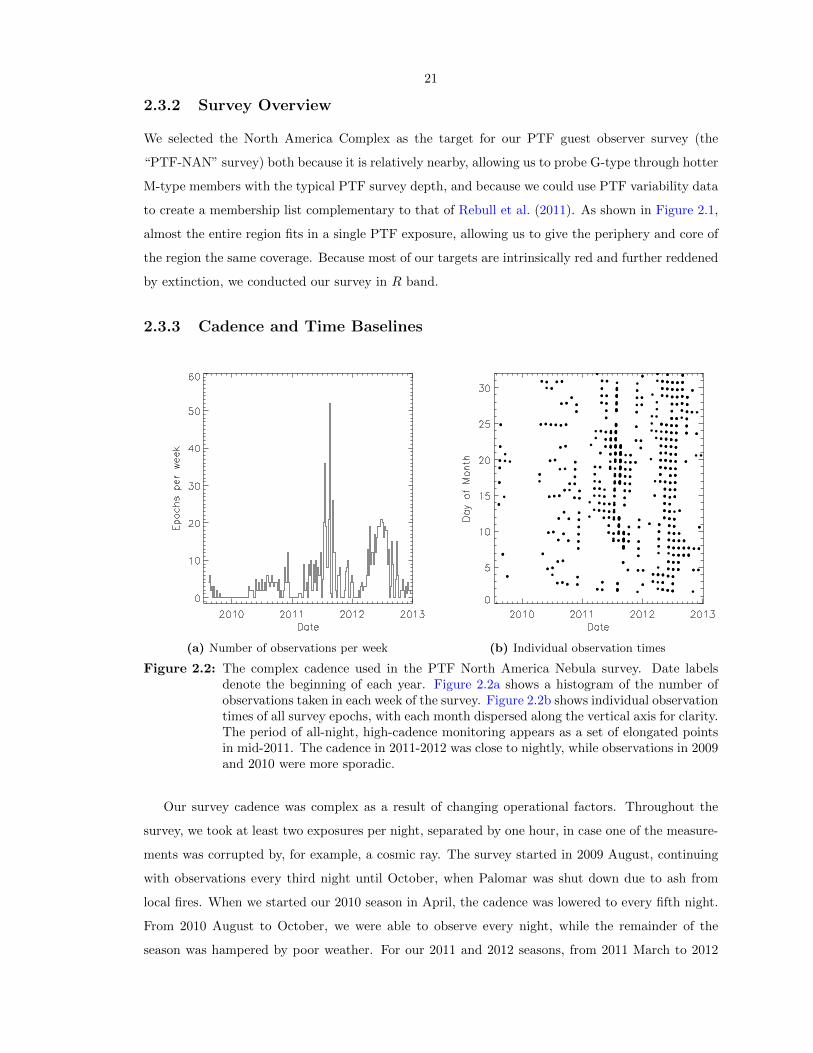
2.3.2 Survey Overview

We selected the North America Complex as the target for our PTF guest observer survey (the

“PTF-NAN” survey) both because it is relatively nearby, allowing us to probe G-type through hotter

M-type members with the typical PTF survey depth, and because we could use PTF variability data

to create a membership list complementary to that of Rebull et al. (2011). As shown in Figure 2.1,

almost the entire region fits in a single PTF exposure, allowing us to give the periphery and core of

the region the same coverage. Because most of our targets are intrinsically red and further reddened

by extinction, we conducted our survey in R band.

2.3.3 Cadence and Time Baselines

(a) Number of observations per week (b) Individual observation times

Figure 2.2: The complex cadence used in the PTF North America Nebula survey. Date labelsdenote the beginning of each year. Figure 2.2a shows a histogram of the number ofobservations taken in each week of the survey. Figure 2.2b shows individual observationtimes of all survey epochs, with each month dispersed along the vertical axis for clarity.The period of all-night, high-cadence monitoring appears as a set of elongated pointsin mid-2011. The cadence in 2011-2012 was close to nightly, while observations in 2009and 2010 were more sporadic.

Our survey cadence was complex as a result of changing operational factors. Throughout the

survey, we took at least two exposures per night, separated by one hour, in case one of the measure-

ments was corrupted by, for example, a cosmic ray. The survey started in 2009 August, continuing

with observations every third night until October, when Palomar was shut down due to ash from

local fires. When we started our 2010 season in April, the cadence was lowered to every fifth night.

From 2010 August to October, we were able to observe every night, while the remainder of the

season was hampered by poor weather. For our 2011 and 2012 seasons, from 2011 March to 2012

22

January and from 2012 March to 2012 December, we were able to observe every night, but only

during bright time, as the PTF project had started observing exclusively with the g′ filter during

dark time. In addition, during 2011 July and August, we obtained hourly exposures all night, in

both bright and dark time. We illustrate our observing pattern in Figure 2.2.

Our survey represents one of the most uninterrupted, multi-year optical variability surveys of

a star-forming region, featuring 894 epochs across 365 nights between 2009 August 13 and 2013

February 22. Our largest data gaps are the 1-3 month gaps in the winter, when the region is not

visible from Palomar, and the two-week gaps during dark time in most months when the R filter is

not available. Aside from these regular gaps, we have two years of uninterrupted nightly coverage,

except for occasional weather gaps, and another year and a half of lower-cadence data for probing

long-term variability.

In addition to the data presented here, PTF continued to observe the North America Nebula

region through 2013 December, although this data set has not yet been fully reduced by the PTF

Photometric Pipeline. PTF will also continue to observe the North America Nebula complex, among

other star-forming regions, at low cadence over the next few years as part of a separate search for

very-long-term variability.

2.3.4 Aliasing

While the focus of our study is on aperiodic variability, we were also able to determine periods for

those sources that were periodic. I analyzed the susceptibility of our cadence to aliasing following

the standard window function formalism.

A series of magnitude measurements (tj , mj), each with negligible exposure time compared to the

timescales of interest, can be expressed as the product of a continuous “real” signal m(t) multiplied

by an observing pattern w(t), where w(t) is a sum over terms δ(t − tj) for each observation. The

Fourier transform ˆm(ν) and power spectrum Pm(ν) of the observed signal can then be expressed in

terms of the Fourier transform of the observing pattern, w(ν) (Deeming, 1975):

ˆm(ν) = m(ν) ∗ w(ν)

Pm(ν) = Pm(ν) ∗ |w(ν)|2

The expression w(ν), known as the window function, convolves the true Fourier transform of the

variability, m(ν), into the observed transform ˜m(ν) in a manner analogous to that in which the

point-spread-function of an instrument convolves the true spatial distribution of incident radiation

into an observed image. The window function therefore determines the quality of power spectra,

periodograms, and other products of Fourier analysis in the same way that a point-spread-function

determines the image quality of an instrument.

23

0.0 0.2 0.4 0.6 0.8 1.0

0.0

0.2

0.4

0.6

0.8

Ν Hday-1L

HΝL¤

2

(a) Frequencies up to 1 day−1

-0.004 -0.002 0.000 0.002 0.0040.0

0.2

0.4

0.6

0.8

1.0

Ν Hday-1L

HΝL¤

2

(b) Frequency-space convolution kernel

0.98 0.99 1.00 1.01 1.020.0

0.1

0.2

0.3

0.4

0.5

Ν Hday-1L

HΝL¤

2

(c) The alias at 1 day−1

Figure 2.3: The squared amplitude of the window function, |w(ν)|2 in the text, as a function offrequency. In all plots, the blue curve represents the window function correspondingto our PTF observations from 2009 through 2012. In Figure 2.3b, the purple curveis the window function that would be achieved in the idealized limit of continuousmonitoring. The observed window function is well-behaved, with no major aliasesaside from the inevitable daily alias.

24

If w(t) has the form∑j δ(t − tj) for observation times tj, then the window function has the

form

w(ν) =1

N

∑j

e−2πitjν (2.1)

The squared amplitude of the window function, |w(ν)|2, is illustrated in Figure 2.3 for the PTF

cadence from 2009 August through 2012 December. The FWHM frequency resolution of our cadence

is 0.00099 day−1, 37% larger than the resolution attainable by a continuous monitoring program over

the same baseline (0.00072 day−1). With this data we can determine 2-day periods to± 0.004 days√SNR

, but

200-day periods only to ± 40 days√SNR

, where SNR denotes the signal-to-noise ratio of the periodogram,

not of the original measurements.

The dominant alias is a pair of peaks at 1 day−1, which reach 56% of the primary peak at w(0).

Therefore, one expects alias peaks in a periodogram to have roughly 56% the height of the associated

true peak, although the exact ratio will vary depending on coincidences with noise fluctuations or

with overtones and other secondary peaks, as well as on how closely a given type of periodogram

is related to Fourier analysis and the power spectrum. Our experience with phasing lightcurves

in the PTF data by various trial periods confirms that, while we can frequently assume that the

highest peak in a Lomb-Scargle periodogram is the true period, the true period corresponds to the

second-highest peak in a fair number of cases.

The exact frequencies of the two daily aliases are 1.000 day−1 and 1.003 day−1. The former

frequency is one per solar day, while the latter frequency is very close to one per sidereal day. We

believe that, while the 1.000 day−1 alias is the ordinary alias resulting from nightly observations, the

1.003 day−1 alias is caused by the scheduling of observations, over the course of the year, for when

the NAN Complex is highest in the sky, which results in observations separated by one sidereal day

on average.

Other aliases include a yearly alias, at 0.003 day−1 and 20% of the height of the primary peak,

and an unexplained alias at 0.102 day−1 (perhaps related to PTF’s operations schedule, as it is close

to one third of a synodic month) but only 4% of the height of the primary peak. In general, the

window function shown in Figure 2.3 is remarkably clean, indicating that the daily alias is the main

caveat in interpreting periodic variability.

2.3.5 Systematics

The PTF Photometric Pipeline has several limitations that must be borne in mind when analyzing

our work. The most important is that, since sources were identified using SExtractor and charac-

terized using aperture photometry, sources may be missing, misidentified, or have poor photometry

in regions with substantial Hα nebulosity. An example of a region with missing sources can be seen

in Figure 2.4.

25

Figure 2.4: An example of a PTF image where not all sources were detected with SExtractor.Red circles mark the positions of SExtractor detections; most of the sources near thenebula filament in the center are not circled. One of the missing sources is PTF10nvg(Covey et al., 2011), which was identified by the LBNL transient pipeline.

26

In addition, the PTF Photometric Pipeline does not use color corrections when computing

(RPTF); these terms are around 0.2 mag per magnitude of r − i (Ofek et al., 2012). The lack

of a color term means that sources with large color changes over the course of their variability will

have their amplitudes slightly overestimated if they get redder as they get brighter, and slightly un-

derestimated if they get redder as they get fainter. Fortunately, it will take a large color amplitude

(∆(r − i) & 0.5) to significantly affect our measured amplitudes. The color term may be a more

significant issue for future work with the PTF data set, once improved reductions allow us to probe

variability below amplitudes of a few tenths of a magnitude.

The pipeline also underestimates photometric errors, even after including a systematic error term

(Levitan & Sesar, priv. comm. 2012).

2.4 Supplementary Data

2.4.1 Spectroscopy

We pursued optical spectroscopy both of stars with significant variability (as selected in subsec-

tion 3.2.1) and of the infrared-excess selected sample of Rebull et al. (2011) using the MMT, Keck

Observatory, Palomar Observatory, and Kitt Peak National Observatory. Several of our targets were

also observed by other members of the PTF collaboration as part of PTF’s spectroscopic follow-up

program.

We observed 257 variable infrared-excess sources in the North America Nebula using the DEIMOS

multi-object spectrograph (Faber et al., 2003) at Keck on 2012 July 18-19 and 2013 July 9, using

the 600 line/mm grating. PTF was monitoring the field during both 2012 nights that spectra were

taken, allowing us to determine the photometric state represented by each spectrum for all stars

except those varying substantially in less than a day.

The DEIMOS spectra were reduced using a modified version of the DEEP2 pipeline (Newman

et al., 2013; Cooper et al., 2012), provided to us by Evan Kirby. The spectra were bias-corrected,

dome-flatfielded, and wavelength-calibrated, but were not flux-calibrated. We corrected for sky and

nebula emission by subtracting the off-source spectrum visible within each slit. The final spectra

covered approximately the 4400-9500 A range at 5 A resolution, although the range covered by the

spectrum of any particular star could shift by ∼ 500 A in either direction depending on the position

of the star’s slit on the instrument mask. Many cosmic rays were left uncorrected by the pipeline,

so when making the figures in Chapter 3, we cleaned the cosmic rays by hand for clarity.

194 sources selected by either variability or infrared excess were observed using the Hectospec

multi-object spectrograph (Fabricant et al., 2005) on the MMT on 2012 November 3, December 4,

and December 6, using the 270 lines/mm grating. The data were pipeline processed at the Harvard-

Smithsonian Center for Astrophysics (Mink et al., 2007). The final spectra cover 3700-9100 A at 6 A

27

resolution. PTF observed the region on November 3 and December 6, but to interpret the December

4 spectra we had to interpolate between photometry from December 3 and December 6.

Lynne Hillenbrand had previously obtained low-resolution optical spectra of sources in the North

America Nebula complex with the HYDRA multi-object spectrograph (Barden et al., 1993) on the

3.5m WIYN telescope at Kitt Peak, using the 316 line/mm grating, on six nights between 1998 June

2 and 1998 July 21. L. H. also took spectra using the (now decommissioned) Norris multi-object

spectrograph (Hamilton et al., 1993) on the 5m Hale Telescope at Palomar, using the 600 line/mm

grating, on 1998 August 14-15, 1999 July 21-23, and 1999 September 2-5. The HYDRA and Norris

spectra do not have concurrent photometry.

The HYDRA and Norris observations were reduced for us by Gregory Herczeg using custom

routines written in IDL. The routines applied corrections for bias, dome flats, cosmic rays, scattered

light, and wavelength calibration. The spectra were not flux-calibrated. Sky and nebula emission

were corrected by taking a shorter sky exposure offset 6-10′′ from the target position, and subtracting

the counts in the sky exposure from the corresponding source spectrum, after scaling to the difference

in observing times. In several configurations the sky emission was scaled by an additional 10-20%

to account for changes in the sky transmission. The HYDRA spectra covered 5000-10000 A at

R ∼ 1, 500, while the Norris spectra covered 6100-8750 A at R ∼ 2, 000.

The PTF collaboration took classification spectra for 12 sources in our field: PTF09dsa, PTF09ejq,

PTF09ekb, PTF09epi, PTF09fuk, PTF10gdb, PTF10geh, PTF10qpf, PTF10suh, PTF10abyb, PTF11cjr,

and PTF11oyt, sometimes at multiple epochs. The PTF spectra are a heterogeneous sample.

Roughly half were taken with KAST on the Lick 3-m, with the remainder divided among LRIS

on Keck, RCspec on the Kitt Peak 4-m, DBSP on the Palomar 200-inch, ACAM on the William

Herschel Telescope, and LRS on the Hobby-Eberly Telescope. The spectra extended from 3500-

4000 A to 8500-10000 A at resolutions of 5-15A.

2.4.2 Mid-IR Photometry

Luisa Rebull provided us with Spitzer photometry for all sources observed for Rebull et al. (2011),

including unpublished photometry for sources that did not have an infrared excess. The data were

reduced as described in that paper. We made use of all four IRAC channels, and the MIPS 24

µm channel, but not the MIPS 70 µm or 100 µm channels. Most of the PTF survey area was also

covered by the Spitzer data (Figure 2.5).

2.4.3 Near-IR Photometry

We supplemented the mid-IR photometry from Spitzer with J, H, and K-band photometry from

the Two-Micron All-Sky Survey (2MASS). 2MASS sources were filtered by the same quality cuts as

28

(a) IRAC 5.8 µm coverage (b) MIPS 24 µm coverage

Figure 2.5: The North America Nebula complex as a Spitzer mosaic (Guieu et al., 2009; Rebullet al., 2011). The red rectangle represents the area covered by Figure 2.1. We haveIRAC data for nearly all sources of the survey region, and MIPS data for a majorityof sources.

adopted by Guieu et al. (2009) and Rebull et al. (2011). Only photometry with band quality flags

of ”A”, ”B”, ”C”, or ”U” was considered (Rebull, priv. comm. 2014).

2.4.4 Hα Fluxes

We used Hα photometry from the INT Photometric H-alpha Survey (IPHAS; Drew et al., 2005) to

characterize the fraction of sources of interest with strong accretion. Since the IPHAS initial data

release appeared to have been withdrawn from publication at the time of writing2, we instead relied

on the source matching carried out by Rebull et al. (2011).

2.5 Summary

Thanks to PTF, we have collected, for the first time, a homogeneous long term, medium-cadence

optical variability survey of the North America Nebula (NAN) complex. While the photometric

precision, cadence, or time baseline have all been individually exceeded by previous surveys, the

combination of factors has given us a unique perspective on pre-main-sequence stellar variability. In

particular, a survey such as PTF-NAN is the only way to comprehensively study aperiodic variability,

as both lower cadences and shorter baselines will miss key components of the variability.

2A new release was published as the thesis was being finalized (Barentsen et al., 2014), and will be incorporatedinto future work.

29

The PTF-NAN survey is supplemented by spectroscopic follow-up observations, as well as optical,

near-infrared, and mid-infrared photometry collected for Rebull et al. (2011). Where available, we

use Hα fluxes from the IPHAS survey to characterize stars for which we were unable to obtain

spectra.

30

2.6 References

Bally, J., & Scoville, N. Z. 1980, ApJ, 239, 121

Barden, S. C., Armandroff, T., Massey, P., Groves, L., Rudeen, A. C., Vaughnn, D., & Muller, G.

1993, in Astronomical Society of the Pacific Conference Series, Vol. 37, Fiber Optics in Astronomy

II, ed. P. M. Gray, 185

Barentsen, G. et al. 2014, ArXiv e-prints, arXiv:1406.4862

Comeron, F., & Pasquali, A. 2005, A&A, 430, 541

Cooper, M. C., Newman, J. A., Davis, M., Finkbeiner, D. P., & Gerke, B. F. 2012, Astrophysics

Source Code Library, ascl:1203.003

Covey, K. R. et al. 2011, AJ, 141, 40, arXiv:1011.2565

Deeming, T. J. 1975, Ap&SS, 36, 137

Drew, J. E. et al. 2005, MNRAS, 362, 753, astro-ph/0506726

Faber, S. M. et al. 2003, in Society of Photo-Optical Instrumentation Engineers (SPIE) Conference

Series, Vol. 4841, Society of Photo-Optical Instrumentation Engineers (SPIE) Conference Series,

ed. M. Iye & A. F. M. Moorwood, 1657–1669

Fabricant, D. et al. 2005, PASP, 117, 1411, arXiv:astro-ph/0508554

Guieu, S. et al. 2009, ApJ, 697, 787, arXiv:0904.0279

Hamilton, D., Oke, J. B., Carr, M. A., Cromer, J., Harris, F. H., Cohen, J., Emery, E., & Blakee,

L. 1993, PASP, 105, 1308

Laugalys, V., Straizys, V., Vrba, F. J., Boyle, R. P., Davis Philip, A. G., & Kazlauskas, A. 2006,

Baltic Astronomy, 15, 483

Law, N. M. et al. 2009, PASP, 121, 1395, arXiv:0906.5350

Levitan, D. et al. 2011, ApJ, 739, 68, arXiv:1107.1209

Mink, D. J., Wyatt, W. F., Caldwell, N., Conroy, M. A., Furesz, G., & Tokarz, S. P. 2007, in Astro-

nomical Society of the Pacific Conference Series, Vol. 376, Astronomical Data Analysis Software

and Systems XVI, ed. R. A. Shaw, F. Hill, & D. J. Bell, 249

Newman, J. A. et al. 2013, ApJS, 208, 5, arXiv:1203.3192

Ofek, E. O., Frail, D. A., Breslauer, B., Kulkarni, S. R., Chandra, P., Gal-Yam, A., Kasliwal, M. M.,

& Gehrels, N. 2011, ApJ, 740, 65, arXiv:1103.3010

Ofek, E. O. et al. 2012, PASP, 124, 62, arXiv:1112.4851

Rau, A. et al. 2009, PASP, 121, 1334, arXiv:0906.5355


31

Chapter 3

Disk-Related Bursts and Fades inYoung Stars1

3.1 Introduction

The best-studied aperiodic variables at present are episodic variables: stars whose lightcurves contain

one or more isolated features that can be explained as accretion or extinction events. The relative

simplicity of episodic variables, along with the scrutiny to which they have already been subjected

in the literature (reviewed in subsection 1.2.3), makes them an excellent starting point for any study

of aperiodic variability as a whole. In addition, bursting and fading have been relatively poorly

studied on timescales of weeks, while our data allows us to explore these timescales very well.

The present chapter focuses on observable optical variability among the ∼ 2, 100 known and

suspected members of the North America Nebula complex cataloged by Rebull et al. (2011) based

on mid-infrared selection techniques. Of these, 84% are within our monitored field. Among the wide

range of behaviors exhibited by variable stars, we consider the evidence for and typical properties of

bursting or fading behavior, possibly mixed with other forms of variability. In the case of bursting

stars, while accretion-related instabilities having timescales of a few tens of days have been predicted

by a number of theoretical studies (e.g., Aly & Kuijpers, 1990; Romanova et al., 2004), no evidence

for accretion bursts produced by such instabilities has been published (Bouvier et al., 2007), although

accretion bursts on both shorter (Murphy et al., 2011) and longer (Herbig, 2008) timescales have been

observed. We assess, for the first time, the frequency of these intermediate timescale instabilities.

For fading stars, while the existence of extinction-related variability is well-established, results vary

among authors as to the frequency of young stars exhibiting such behavior, as well as the typical

timescales. We also address in this study, for the first time, the ratio of bursting to fading lightcurves

for a typical T Tauri star population.

The remainder of this chapter is organized as follows. In section 3.2, we present our photometric

1Based on work published as Findeisen et al. (2013), ApJ 768, 93. c© 2013. The American Astronomical Society.All rights reserved. Material has been edited for presentation within a thesis.

32

data and our detection thresholds for variability. Section 3.3 discusses how we defined the burster

and fader populations and their key properties. In sections 3.4 and 3.5, we discuss the bursters and

faders in more detail, with an emphasis on how the largest sample yet identified of such objects

can constrain their underlying physics. In section 3.6, we describe several noteworthy objects in

more detail. Section 3.7 summarizes our results, describes limitations of our analysis, and suggests

pathways for future work.

3.2 Photometric Data

This study was based on PTF data collected between 2009 August and 2012 December, as described

in subsection 2.3.3, and reduced by the PTF Photometric Pipeline, as described in subsection 2.2.2.

The original sample selection was based on a less complete data set, through 2012 April, and some

sources that were originally in our sample fell outside our selection criteria when the remaining

months were included. For consistency, these sources were kept inside the sample.

3.2.1 Identifying the Variables

To determine which sources were variable during the observation period, we grouped all PTF de-

tections with 14 ≤ R ≤ 20 mag into half-magnitude bins on a chip-by-chip basis. The width of the

bins (0.5 mag) was chosen so that the brightest and least populated bin (14-14.5 mag) had roughly

100 sources on most chips. We then computed the median RMS of all the stars in each bin, and fit

the medians by an equation of the form:

RMS =√a2 + (b× 10−0.4p(mag−14))2 (3.1)

This equation is partly motivated as the sum of a systematic term and a flux-dependent term; the

exponent of the flux-dependence p was allowed to vary because the natural choice, p = 12 (i.e., noise

that scales as the square root of the flux, as expected from photon noise), was too shallow. In

practice we found p ∼ 23 for most chips. We list the fit parameters in Table 3.1.

The curve found by fitting Equation 3.1 describes the locus of nonvariable stars on a given chip.

We defined the boundary between variable and nonvariable stars to be 1.75 times the median RMS.

This cutoff was determined empirically, rather than analytically, to avoid making assumptions about

the noise properties of the data. We set the cutoff by visually inspecting lightcurves with both R ∼ 14

and R ∼ 16; at RMS values lower than 1.75 times the threshold the lightcurves were indistinguishable

from noise, while at higher values the lightcurves were clearly structured on short timescales.

We show in Figure 3.1 plots of RMS vs. magnitude for the six chips that covered the star-forming

complex, along with the median fit and the variability detection boundary for each chip. For 14th

33

Figure 3.1: RMS scatter vs. median magnitude for all sources with flags (listed in subsection 2.2.2)in fewer than half the epochs. The fit to the median RMS as a function of magnitudeis plotted as the lower red curve, while our variability detection threshold (1.75 timesthe median) is plotted as the upper red curve. X’s mark candidate bursting stars fromTable 3.4 while squares mark candidate fading stars. 27 high-amplitude variables arebeyond the upper edge of the Chip 0 plot, 10 each above the upper edge of the Chip 1and Chip 2 plots, and 1-5 off the upper edge of each of the others.

34

Chip a b p Total Sources Variables0 0.033 0.0053 0.68 6,090 491 (8.1%)1 0.018 0.0130 0.52 9,330 490 (5.3%)2 0.023 0.0145 0.49 14,057 533 (3.8%)6 0.026 0.0072 0.62 11,036 457 (4.1%)7 0.025 0.0081 0.60 7,720 337 (4.4%)8 0.022 0.0105 0.55 10,393 397 (3.8%)

Table 3.1: Best-fit values for the parameters in Equation 3.1 for each of the six target chips. Theparameter a can be interpreted as the systematic noise floor at bright magnitudes, and pis the power-law dependence of RMS on flux at faint magnitudes. The last two columnsshow the total number of PTF sources on each chip as well as the number selected bymaking an RMS cut at 1.75 times the value given by Equation 3.1.

magnitude stars, we are sensitive to variability with an RMS amplitude of a few percent, while

below 16th magnitude, we can probe only 10% flux variations. In Table 3.1, we list the number of

PTF sources and the number and fraction identified as photometrically variable using the methods

outlined above. Nearly 3,000 variables projected on the dark cloud and the associated nebulae are

identified. Their RMS amplitudes range from 0.03 to 1.1 mag.

3.3 Bursting and Fading Among Infrared Excess Sources

3.3.1 Sample Selection

Because the North America Nebula complex is located in the plane of the Galaxy, a significant

number of our high quality lightcurves are those of foreground or background field stars. In our

first reconnaissance of the variability properties of the region, we therefore concentrated on variable

stars among a list of candidate North America Nebula members identified by Rebull et al. (2011).

Specifically, Rebull et al. used infrared colors, primarily Spitzer IRAC 3.6 µm − MIPS 24 µm,

to identify stars surrounded by circumstellar dust. Additional considerations included location

in various color-magnitude diagrams that help distinguish young stars from contaminating dusty

sources such as extragalactic AGN and galactic late-type giants. Each source was assigned a spectral

energy distribution class based on the slope of a linear fit to all available photometry between 2 and

24 µm. Class I sources have rising slopes and are interpreted as objects with not only circumstellar

disks, but likely more spherically distributed envelopes as well. Flat-spectrum sources have roughly

constant λFλ over the 2-24 µm range and have a similar interpretation. Class II sources are consistent

with traditional disk SEDs. Class III sources have the steepest slopes; most have no excess in the

IRAC bands but were selected based on an excess at 24 µm. Only 6 of the Class III sources in

Rebull et al. (2011) were not selected using either IRAC or MIPS excess criteria. Rebull et al. note

that, since their primary selection is based on infrared data, they are incomplete with respect to

Class III sources.

35

IR Source Type # in RGS2011 in PTF Field PTF Counterparts With R < 18 Flags in < 50% Epochs High RMSMIPS-Only 25 25 (100%) 0 ( 0%)Class I 273 242 ( 89%) 11 ( 5%) 3 (27%) 3 (100%) 3 (100%)Flat-Spectrum 272 242 ( 89%) 53 (22%) 20 (38%) 13 ( 65%) 10 ( 77%)Class II 604 542 ( 90%) 321 (59%) 160 (50%) 120 ( 75%) 79 ( 66%)Class III 112 82 ( 73%) 76 (93%) 43 (53%) 31 ( 72%) 16 ( 52%)IRAC-Only 796 613 ( 77%) 140 (23%) 27 (19%) 19 ( 70%) 9 ( 47%)Total 2,082 1,746 ( 84%) 601 (34%) 253 (42%) 186 ( 74%) 117 ( 63%)

Table 3.2: Rebull et al. (2011) gave SED classes only for sources that were detected in both IRACand MIPS. Sources that were detected in only one or the other are listed for comparison,but were not used to estimate the incompleteness from source confusion and flux limits.

Of the 2,082 candidates from Rebull et al. (2011), 601 had a counterpart in the PTF source

catalog. As we show in Table 3.2, the recovery rate by PTF depended strongly on the type of IR

excess. Only 5% of the relatively red Class I sources in the PTF field had detections, while fully

93% of the relatively blue Class III sources were detected by PTF. The strong correlation between

(infrared) source color and recovery rate, in the sense that redder sources are recovered less often,

suggests that most of the sources we did not recover in PTF were missed because they were below

our optical detection limits. However, from image inspection we also know that the PTF pipeline

had difficulty identifying and extracting sources from crowded or nebulous regions. If we assume

that all the Class III sources must be bright enough to detect in the optical if they are visible in the

Spitzer bands even with a small infrared excess, then source extraction problems should dominate

the 7% missing Class III sources. Presumably, roughly 7% of the rest of the sample also fell in regions

where the PTF pipeline could not reliably identify sources. This argument assumes that Class III

sources are not less likely to be in crowded or high-background regions, where the PTF pipeline is

least reliable, and should be treated with caution. We note that, while the overall incompleteness

does not affect our main science goals, the bias away from Class III sources in the parent sample

and the bias away from Class I sources from cross-matching to PTF do limit our ability to examine

how variability properties change with the degree of infrared excess.

From our sample of 601 infrared excess selected candidate members with PTF counterparts,

we restricted our attention to the 253 sources brighter than a median RPTF = 18. The detailed

breakdown by SED type is given in Table 3.2. We found from experience that the photometric

quality for sources fainter than RPTF ∼ 18 was such that, while we could determine whether a

source was variable, we could not consistently assess the structure of the variability. Considering

only sources whose lightcurves had bad photometry flags (see subsection 2.2.2 for a list) in fewer

than half the epochs further reduced the sample to 186 stars, which are shown in Figure 3.2. The

figure shows no trend with RPTF except for more sources at fainter magnitudes, suggesting our

magnitude limits avoid any substantial systematics. High-amplitude sources (RMS & 0.3-0.4 mag)

tend to be associated with strong infrared excess, while low amplitudes are found in both strong-

and weak-excess sources.

36

Figure 3.2: PTF magnitude and IR color distributions for those PTF sources that have an in-frared excess from Rebull et al. (2011) and whose lightcurves have flags (listed insubsection 2.2.2) in fewer than half the epochs. The color of the dots indicates thedegree of infrared excess: blue dots are class III sources, green ones class II, yellowones have a flat IR spectrum, while magenta sources are class I sources. The blacksources are those that were not detected in the Spitzer 24µm band, and so did nothave an IR excess class listed in Rebull et al. (2011). Not all sources appear on bothplots, as some had missing 8µm or 24µm photometry. The curves in the upper leftpanel show synthetic photometry of Siess et al. (2000) isochrones for ages of 2 Myr(red) and 100 Myr (blue), at a distance of 600 pc, indicating the expected colors ofstars with no infrared excess at all. As in Figure 3.1, X’s mark candidate burstingstars while squares mark candidate fading stars.

37

Figure 3.3: RMS distribution of the sample, and its correlation with the presence of Spitzer infraredexcess. Left: the fraction of sources with an infrared excess out of all PTF sourceswith 13.5 ≤ R ≤ 18 and flags (listed in subsection 2.2.2) in fewer than half the epochs.Right: the solid line denotes the distribution of RMS amplitudes for the 186 infraredexcess sources from Rebull et al. (2011) whose lightcurves have flags in fewer than halfthe epochs. The dashed line represents the subset of 117 that lie above the variabilitythresholds in Figure 3.1.

From this sample of 186, we studied in more detail the 117 that showed significant variability

in PTF, as defined in subsection 3.2.1. Both cuts are presented in more detail in Table 3.2. These

infrared excess selected variables include most of the high amplitude variables in the field, as shown

in Figure 3.3; most of the low amplitude variables in the field lack an infrared excess and are not

part of our sample. The 117 infrared-excess variable sources, along with the other variables in the

field, exhibit a wide range of timescales and amplitudes in their lightcurves. We sought to categorize

the lightcurves and hereafter we focus on those that can be identified as bursting or fading.

When selecting sources for inclusion on the list of bursters or faders, we defined a burst in a

lightcurve as a period of elevated fluxes above a (local) floor of relatively constant brightness. We

did not place any explicit restriction on the length of the candidate burst. However, we tended to

require elevated fluxes in multiple consecutive epochs to be certain that a brighter measurement was

not a measurement error, and we required that the period of elevated fluxes be short enough that

we could recognize the remainder of the lightcurve as a well-defined “quiescent” state. We defined

fades analogously as a period of lowered fluxes, with the caveats that we believed the lower fluxes

represented real variability and that the lower fluxes were distinct from the normal variability of

the star. Both definitions were necessarily subjective, and we review possible selection effects in

subsection 3.7.3.

38

We visually inspected all 117 lightcurves for bursting or fading activity. For comparison, we also

inspected 100 randomly chosen variable PTF sources that did not have an infrared excess, mixing

them with the sample of 117 so that we did not know whether any particular lightcurve was from

the target sample or the control group. We designated a star as a burster or a fader if it had at least

one bursting or fading event during the monitoring period.

3.3.2 Burster and Fader Statistics

We identified 14 stars with candidate bursts and 29 stars with candidate fades, with two stars showing

both bursting and fading behavior. The sources are listed in Table 3.3, with their photometric

behavior summarized in Table 3.4. Lightcurves of all 41 stars are available online from the PTF

website2. The sources are also highlighted in Figures 3.1, 3.2, and 3.4.

For comparison, in the control group of 100 sources with no infrared excess, we saw only two

stars that appeared to have one burst each, and no faders other than eclipsing binaries. The burst

detected in one of the stars turned out to be a transient scattered light artifact we had failed to spot

at the time of the original analysis. The other may also have been identified as a burster because

of a systematic error in the data or in our visual inspection, or it may represent real astrophysical

variability in the field. In the former case we expect ∼ 2 of the bursters in our target sample to be

mislabeled, while in the latter we expect ∼ 1 false positives.

The stars listed in Tables 3.3 and 3.4, some of which are highlighted in Figure 3.5 and Figure 3.6,

show a wide variety of behaviors. We see variability from a few tenths of a magnitude to several

magnitudes. The bursts or fades last anywhere from around a day, the shortest timescale resolvable

in most of our data, to hundreds of days. Events may repeat as frequently as once a week, or

can appear only once in the three-year monitoring period. Nearly all the bursters and faders are

aperiodic, with the exception of two faders that are discussed further in section 3.5.

3.3.3 Spectroscopic Characterization

We pursued optical spectroscopy of both the variable star selected sample (this paper) and the

infrared-excess selected sample of Rebull et al. (2011) using the MMT, Keck Observatory, Palomar

Observatory, and Kitt Peak National Observatory.

Of the spectroscopic samples described in subsection 2.4.1, the 2012 DEIMOS observations in-

cluded 19 bursters or faders, and the MMT observations included 22 bursters or faders. The HYDRA

and Norris spectra taken in 1998 and 1999 included 27 bursters or faders.

2http://www.astro.caltech.edu/ptf/

http://www.astro.caltech.edu/ptf/

39

Figure 3.4: The North America Nebula complex, as observed by PTF in a single epoch from 2009.The blue circles mark the positions of candidate members selected using infrared excessby Rebull et al. (2011). As in Figures 3.1 and 3.2, we highlight stars with apparentbursting activity with red X’s, and stars with apparent fading activity with red squares.

40

(a) 0.2 mag amplitude (b) 2.5 mag amplitude

(c) 2-day duration (d) 160-day duration

(e) 10-day separation (f) 1-year separation

Figure 3.5: Examples of the diverse behavior seen in our lightcurves for bursting stars. Variabilityamplitudes range from a few tenths of a magnitude to 2 magnitudes. Detected burstscan last from less than two days to over a hundred, and can be separated by anywherefrom 10 days to a year. For scale, the horizontal bar near the top of each panel shows a10 day interval. No points having any of the flags listed in subsection 2.2.2 are plotted.

41

(a) 0.4 mag amplitude (b) 2.3 mag amplitude

(c) 1 day duration (d) >1 year duration

(e) 9 day separation (f) 1 year separation

Figure 3.6: Examples of the diverse behavior seen in our lightcurves for faders. Variability ampli-tudes range from a few tenths of a magnitude to nearly 2 magnitudes. Fades can lastanywhere from one day to over a year, and can be separated by anywhere from 9 daysto over a year. For scale, the horizontal bar near the top of each panel shows a 10 dayinterval. No points having any of the flags listed in subsection 2.2.2 are plotted.

42

3.4 The Burster Phenomenon

3.4.1 Population Properties

Upward excursions in young star lightcurves traditionally have been assumed to come from one of

two mechanisms. Long-lasting, several-magnitude events in young stars with circumstellar accretion

disks (e.g., EX Lup, FU Ori) are interpreted as dramatic increases in the accretion rate from the

disk to the star. Events lasting a few hours or less and rising by at most a few tenths of a magnitude,

particularly in disk-free stars, have been assumed to be associated with magnetic flares like those

seen on the young field star UV Cet or on the Sun. White light flares on the Sun last tens of

minutes, while those on M dwarfs last up to several hours (e.g., Kowalski et al., 2010; Kretzschmar,

2011). As these timescales are set by the cooling times of dense chromospheric material at the base

of the coronal loop, it is unlikely that magnetic flares can produce optical emission with much longer

durations than observed.

Of the 14 stars that show bursting behavior, only two, [OSP2002] BRC 31 8 and FHO 1, have

bursts lasting 1-2 hours, short enough to be plausible flares. The remainder must be driven by

temporary increases in accretion, drops in extinction, or some other phenomenon. The bursters

show a wide variety of behaviors. None are strictly periodic, although [OSP2002] BRC 31 8 and

FHO 29 do show enhanced photometric activity at roughly 300-day intervals. Some bursters, like

FHO 26, repeat every few weeks. Others, like LkHα 185 or FHO 4, show bursts only once a year

or even more rarely. While [OSP2002] BRC 31 8 and FHO 1 have very short bursts, too brief to

resolve outside our highest-cadence monitoring in mid-2011, FHO 17 featured a burst lasting over

100 days, and FHO 18 showed bursts with a range of lengths from a few days to two weeks.

Despite their variety, the bursters do not fall naturally into distinct subclasses, forming instead

a continuum of behaviors. We show in Figure 3.7 the joint distributions of burst amplitudes, burst

widths, and burst separations for all 14 bursters. To avoid systematics associated with separating a

burst or fade from the surrounding, sometimes complex, variability, and to avoid complications from

varying sampling from event to event, the timescales and amplitudes in Figure 3.7 were estimated

by eye and should be taken as illustrative values only. There is no pattern visible in the plot aside

from a rough trend where longer bursts tend to be separated by longer intervals. The absence of

distinct groups of bursters suggests that the diversity of sources can be explained by continuously

varying the parameters of a single common scenario, rather than by invoking different mechanisms

or different configurations for short- and long-timescale bursters.

If either enhanced accretion or reduced extinction are responsible for bursting events, then stars

with large infrared excess, and therefore more circumstellar material, may be more likely to show

bursting behavior than stars with small infrared excess. Using the Kendall’s τ statistic (Kendall,

1938), we found no evidence for a correlation between the Spitzer IRAC/MIPS [3.6] − [24] color

43

Figure 3.7: Plots of the characteristic amplitudes and timescales for bursters (left) and faders(right), illustrating the wide variety of observed events. The plus signs indicate sourcesthat have either well-defined fixed values for their amplitudes and timescales (such asthe two periodic AA Tau analogs in the lower left corner of the fader panels), orthat have only a single measurement (such as the single-event sources in the upperright of any panel). The ellipses represent sources that have bursts or fades of varyingamplitudes, varying widths, or varying separations within a single lightcurve. The areabelow the dotted line on the lower two figures, where events would need to overlap eachother, is not allowed, though some ellipses appear there because this analysis does notconsider correlations between width and separation.

44

(56% confidence) and the presence of bursting among our sample of 117 IR-excess sources, but we

did find a marginally significant correlation (2.4% confidence) with Spitzer IRAC [3.6]− [8.0] color,

in the sense that redder sources are more likely to show bursting behavior. We note that of the 14

bursters, only two, FHO 2 and FHO 24, are Class III sources. The rest have K − [8] > 1.8 and

K − [24] > 5 (see Figure 3.2 for comparison to the rest of the sample). We note that since the

K-band and Spitzer data are not coeval, the reported colors may be distorted by variability between

the epochs of observation. However, mid-infrared variability is typically a few tenths of a magnitude

or less (Espaillat et al., 2011; Morales-Calderon et al., 2011; Flaherty et al., 2012), and so should

not dramatically affect a star’s position in diagrams such as Figure 3.2.

While the weak correlation with [3.6] − [8.0] color suggests that bursters are associated with

stronger circumstellar disks, and therefore with the possibility of enhanced accretion or reduced

circumstellar extinction, the absence of a similar correlation with [3.6] − [24] color weakens this

result. As noted in Table 3.3.1, however, only a limited range of infrared color is well-represented

in this sample. It is also possible that any correlation is being diluted by radiative transfer effects,

geometry, or other factors that determine whether any particular star shows bursting behavior. We

discuss how additional data could allow more conclusive tests in subsection 3.7.3.

3.4.2 Constraints on Short-Term Accretion Outbursts

Magnetic or viscous instabilities acting at the boundary between the stellar magnetosphere and

the circumstellar disk are expected to produce short bursts of accretion on timescales of weeks to

months for certain regimes of disk properties (e.g., Aly & Kuijpers, 1990; Goodson & Winglee, 1999;

Romanova et al., 2004, 2005). However, variability from such outbursts has never been observed

(Bouvier et al., 2007). The consistent cadence and long time coverage of our PTF survey have

allowed the most sensitive search to date for such accretion events.

Of the bursting sources in Table 3.4, FHO 2, FHO 4, and FHO 24 show multiple bursts lasting

tens of days each. The separations between bursts vary: tens of days in the case of FHO 24, 100-

300 days in the case of FHO 2, and ∼ 500 days for FHO 4. We show all three sources in Figure 3.8.

The timescales and shapes of these events, particularly FHO 2 and FHO 4, resemble the simulated

variations in M shown in Figure 4 of Romanova et al. (2004). Although they do not stand out in

the context of our sample, where burst durations vary continuously from < 1-150 days, FHO 2,

FHO 4, and FHO 24 are noteworthy as the first bursts reported in young stars having timescales

of tens of days. To our knowledge, these lightcurves represent the first observations consistent with

the predicted inner-disk instabilities.

Models predict that short-term accretion outbursts should have amplitudes of a few tenths of

a magnitude. For example, scaling to a fiducial star with 0.8 M and 2 R, the simulations

of Romanova et al. (2004) predict an accretion rate of 2 × 10−8 Myr−1 in quiescence and 6-

45

Figure 3.8: Burst profiles for three bursters with durations of tens of days. No points having any ofthe flags listed in subsection 2.2.2 are plotted. In this and subsequent plots, the pointsare connected by line segments to clarify the order of closely spaced observations.FHO 2 has the simplest event profile, showing a smooth rise and fall over a 20-30 dayinterval. The bursts of FHO 4 are longer and show a more complex profile. Thelightcurve for FHO 24 shows a large number of contiguous bursts rather than a fewisolated events like the other two.

46

8 × 10−8 Myr−1 in outburst. The fiducial star would have a luminosity of 1.14 L (Siess et al.,

2000), with quiescent and outburst accretion luminosities of 0.25 L and 0.88 L, respectively,

implying a brightening of ∼ 0.4 magnitudes between quiescence and outburst. The three candidate

stars have amplitudes between 0.2 and 0.5 mag, consistent values given star-to-star variations in

star and disk parameters.

The behavior of the lightcurves is inconsistent with white-light flares analogous to those seen on

the Sun. White-light flares tend to have a steep rise followed by an exponential decay. None of the

three bursts show an exponential profile, and the timescales of tens of days are much longer than

the minutes to hours durations observed in the Sun or in low-mass stars. A superposition of many

short flares is also unlikely: FHO 2 and FHO 24 show little variability on timescales of a single day,

as might be expected from a stochastic sum of shorter events. In addition, a 0.4 mag burst lasting

30 days corresponds to an energy release, depending on the (unknown) spectrum of the transient

emission, of ∼ 6× 1039 erg for a 1.4 L star. The entire stellar magnetic field, integrating a dipole

field from an assumed R? ∼ 2 R to infinite radius, contains only ∼ 5 × 1038 (Bsurf/1 kG)2

erg.

Even a 3 kG field, near the largest values observed in T Tauri stars (Bouvier et al., 2007), cannot

provide enough energy to power the bursts.

The brightness enhancements for these three objects are also unlikely to be dust-clearing episodes.

Only FHO 4 is a Class II source, while FHO 2 and FHO 24 are both Class III sources with excess only

in the MIPS 24 µm band. It is doubtful that these two stars have enough circumstellar dust in the

inner disk to allow significant extinction-driven variability. We note that stars with infrared excess

only in the MIPS bands can still show ongoing accretion on the order of 0.1-0.5 × 10−8 M yr−1

(Muzerolle et al., 2009; Espaillat et al., 2012), so the absence of an IRAC excess does not rule out

either low-level accretion or, plausibly, brief periods of accretion at a higher rate. Extinction is a

possible origin for the variability of FHO 4; color data taken over the course of one of its bursts

could test this hypothesis.

3.5 The Fader Phenomenon

The two prototypical faders are AA Tau, which fades repeatedly by 1.4 mag over 30% of an 8.2-day

cycle (Bouvier et al., 1999, 2003), and UX Ori, which fades by 3 mag for tens of days at irregular

intervals (Waters & Waelkens, 1998). Both AA Tau and UX Ori are well understood as the result of

recurring extinction by circumstellar material, from a warped inner disk edge in the case of AA Tau

or from more irregular structures in the case of UX Ori.

Of the 29 sources that show some kind of fading behavior, only two, LkHα 174 and FHO 12,

show the periodic modulation characteristic of AA Tau. Four more sources, LkHα 150, FHO 7,

FHO 15, and FHO 27, show multiple fading events with durations of tens of days, as seen for

47

UX Ori stars. However, their typical amplitudes of 1 mag or less are much smaller than the 3-4 mag

fades associated with UX Ori stars.

The remaining 23 faders do not resemble either of the previously established categories. The

natural assumption is that these sources also have their variability dominated by circumstellar

extinction, with different spatial scales or different geometries causing the lightcurves to behave

differently.

All the sources except for the two AA Tau analogs are aperiodic, and, as illustrated in Figure 3.6,

they often bear little resemblance to each other. For example, FHO 19 has narrow fades repeating

every 8-10 days, but without enough coherence to be periodic. In contrast, NSV 25414 and FHO 3

both have frequent but irregular events, with the interval between adjacent fades varying by more

than a factor of two. At the other extreme, FHO 21 and FHO 22 each show only one fading event

per year, while LkHα 150 and FHO 25 fade only once in the entire survey period. Most fading events

are short, but those of LkHα 150 and [OSP2002] BRC 31 1 last for hundreds of days. Most stars

have fading events of roughly constant depth, but FHO 15 and FHO 20 have significant amplitude

variability. Most fading events are symmetric, but FHO 11 and FHO 27 show strongly lopsided

events.

Like the bursters, the faders do not separate naturally into sources with distinct timescales. We

show in Figure 3.7 the joint distributions of fade amplitudes, fade widths, and fade separations

for all 29 faders. The absence of gaps in the plot suggests that, as with the bursters, short- and

long-timescale faders have a common origin.

As with the bursters, we tested for a correlation with the presence of circumstellar material.

Using the Kendall’s τ statistic, we found no evidence for a correlation between the Spitzer IRAC

[3.6] − [8.0] or IRAC/MIPS [3.6] − [24] colors and the presence of fading among our sample of 117

IR-excess variables at 20% and 18% confidence, respectively. However, we did not find a single

example of a fader among Class III sources (i.e., significant excess only at 24 µm), as would be

expected if circumstellar material near the star is needed for fading events to occur.

To test whether the fading events could instead be the result of variable foreground extinction, we

searched for a correlation between stars’ near-infrared color, where we can avoid variability-induced

systematic errors through the use of coeval 2MASS photometry, and the presence or absence of

fading behavior. Since unreddened M dwarfs have J − K . 1, stars with 1 . J − K . 3 must

have significant extinction, while stars with J − K < 1 may have only moderate extinction. If

fading events are caused by foreground dust, we might expect fading to be more prevalent among

the reddest stars. Using the Kendall’s τ statistic, we found no evidence for a correlation between

the J − K color and the presence of fading among our sample of 117 IR-excess variables at 26%

confidence.

While we find that neither the degree of infrared excess nor proxies for near-infrared reddening

48

are good predictors for the presence of fading behavior, the absence of faders among the Class III

sources is consistent with fading events requiring the presence of inner disk dust and therefore the

possibility of occasionally enhanced extinction along the line of sight. We discuss how additional

data could allow more conclusive tests in subsection 3.7.3.

3.6 Individual Sources of Interest

In section 3.4 and section 3.5 we examined the 41 burster or fader candidates as an ensemble.

However, many of the sources have a character of their own. While we present brief descriptions

of all the sources in Table 3.4, in this section we focus on a small number of stars whose behavior

seems particularly difficult to explain. We present the available data on each and challenge interested

readers to develop models for these sources.

3.6.1 FHO 26

FHO 26 showed several-day-long, ∼ 0.7 mag bursts in 2010 and 2011 (see upper right panel of

Figure 3.9) but became quiescent in late 2011. In 2012, except for two brief bursts, it has shown

only a 0.2 mag, 5.6-day periodic modulation. The 2010-2011 bursts do not phase up under the 2012

period. FHO 26 has a modest infrared excess, as shown in the lower left panel of Figure 3.9.

We show in the lower right panel a spectrum of the source taken in 2012 July, well into the quies-

cent phase and near the peak of the periodic variability. The spectrum shows an M4.5 photosphere

with emission from Hα (-13 A equivalent width).

3.6.2 [OSP2002] BRC 31 1

[OSP2002] BRC 31 1 grew fainter by nearly three magnitudes between 2011 April and August but

showed relatively little variability before the fade, as shown in the upper left panel of Figure 3.10.

Our spectrum, taken during the star’s faint state, shows a forest of emission lines including Hα,

Ca II, [O I], [Fe II], [S II], [Ni II], Fe II, and many others. A spectrum of [OSP2002] BRC 31 1 from

1998 shows only Hα, Ca II, and Fe II at the same strength as in 2012, plus much weaker [O I] and

[Fe II] lines. We see few absorption lines in the spectrum in either epoch.

The 1998 and 2012 spectra are similar to high- and low-state spectra, respectively, of the long-

term variable PTF10nvg (Hillenbrand et al., 2013). Since BRC 31 1, like PTF10nvg, is a Class I

infrared excess source, it is possible that BRC 31 1 is a similar system: a high-inclination source

with circumstellar material obscuring the inner disk, stellar photosphere, and accretion zone, but not

obscuring a spatially extended jet. We note the lightcurve resembles that of V1184 Tau presented

by Grinin et al. (2008).

49

Figure 3.9: A star whose regular bursting activity stopped at the end of 2011. The upper leftpanel shows the full 3-year lightcurve, with the shaded period expanded in the upperright panel to illustrate typical bursts for this source and the vertical red line markingthe time at which the 2012 July spectrum in the lower right panel was taken. Thered scale bar represents a 10-day interval. No points having any of the flags listed insubsection 2.2.2 are plotted. The lower left panel shows the spectral energy distributionfor this source. The points are taken from non-simultaneous optical, near-infrared,and Spitzer photometry. The solid curve is a reddened NextGen model atmosphere(Hauschildt et al., 1999) with temperature corresponding to the star’s spectral type,matched to the optical through J-band fluxes.

50

Figure 3.10: Same as Figure 3.9, but for a star showing a sudden decline in 2011. The star was notdetected in roughly half the epochs in 2012; the non-detections are not shown. Theupper right panel highlights the decline, including a temporary dip that interruptedit. Since we could not determine a spectral type for this source, the photosphereshown in the lower left panel is for an assumed effective temperature.

51

3.6.3 FHO 18

Figure 3.11: Same as Figure 3.9, but for a star showing an odd combination of bursting and fading.The upper right panel shows the fades and their precursor bursts.

FHO 18, shown in the upper panels of Figure 3.11, faded twice by 0.6 mag in quick succession

in 2011. Immediately before each fading event, it brightened by 0.3 mag (upper right panel). This

behavior was not repeated for other fading events during our monitoring period. Aside from these

two fades and their precursor bursts, FHO 18 appears to be a typical Class II young star.

Our DEIMOS spectrum of FHO 18 was taken during a 0.4 mag fade. The spectrum shows a K5

star with Hα emission (-23 A equivalent width) as well as weaker Ca II and He I emission. However,

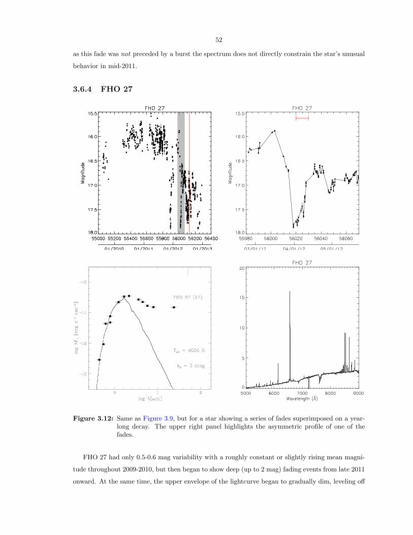
52

as this fade was not preceded by a burst the spectrum does not directly constrain the star’s unusual

behavior in mid-2011.

3.6.4 FHO 27

Figure 3.12: Same as Figure 3.9, but for a star showing a series of fades superimposed on a year-long decay. The upper right panel highlights the asymmetric profile of one of thefades.

FHO 27 had only 0.5-0.6 mag variability with a roughly constant or slightly rising mean magni-

tude throughout 2009-2010, but then began to show deep (up to 2 mag) fading events from late 2011

onward. At the same time, the upper envelope of the lightcurve began to gradually dim, leveling off

53

in mid-2012 after a total decrease of roughly 0.8-0.9 mag. The minimum magnitude reached during

each fading event rose from 17.9 in the first fade to 17.3 in late 2012, so that the most recent fades

have only a few tenths of a magnitude depth.

While the fading events repeat every 30-90 days, they are not periodic. In addition, each fade

has a dramatically different profile from those before and after, with many of the profiles showing

strong asymmetries (Figure 3.12, upper right panel), and some fades being much shallower than the

rest (e.g., a 0.3 mag fade in late 2012 April was sandwiched between a 1.1 mag and a 0.6 mag fade).

The spectral energy distribution of the source, shown in the lower left panel of Figure 3.12, has

a strong infrared excess; Rebull et al. (2011) classify FHO 27 as a flat-spectrum source.

We acquired one spectrum of FHO 27 in 2012 July, during the star’s long-term low state but

between the deeper fading events. The K7 spectrum in the lower right panel of Figure 3.12 shows

strong Hα (-80 A equivalent width), Paschen series, and Ca II emission. Weaker lines in the spectrum

include He I, [O I], and O I.

3.6.5 FHO 28

Like FHO 27, FHO 28 was dominated by 0.6 mag irregular variability in the first few years of

our survey, interrupted by occasional 1 mag fades. Then, in early 2012, it began showing rapid

variability with the same maximum brightness, but with a much higher amplitude of 2 mag. The

high-amplitude variability lasted 130 days before the star returned to its earlier behavior. Since

the source was not strictly periodic during its high-amplitude phase, it is not clear whether the

variability has been fully resolved at our daily cadence, in which case the fades are roughly 9 days

apart, or whether we are seeing a strobing effect of a more rapid 23-hour variation. The lightcurve

is shown on the top two panels of Figure 3.13.

The spectral energy distribution, shown in the lower left panel of Figure 3.13, shows a Class II

infrared excess. A spectrum of FHO 28 (Figure 3.13, lower right panel), taken during its strongly

varying phase, shows an M3 star with strong Hα emission (-60 A equivalent width) and weak Ca II

lines. An older spectrum shows that Hα was much weaker (-20 A) in 1998, although since we don’t

know the photometric state of FHO 28 at the time, it is not clear whether the difference between

the two spectra is related to the star’s increased activity in 2012.

FHO 28 is yet another example of how the photometric behavior of young stars can change

abruptly from one year to the next. This source would not be classified as a fader if we had only

data from its active phase, as the photometry shows no preference between high and low magnitudes

(Figure 3.13, upper right panel). It is the comparison to previous years that allows us to establish

that the brighter magnitudes represent the unperturbed state of the star.

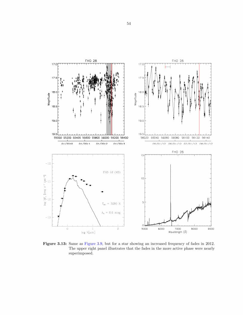
54

Figure 3.13: Same as Figure 3.9, but for a star showing an increased frequency of fades in 2012.The upper right panel illustrates that the fades in the more active phase were nearlysuperimposed.

55

3.7 Summary and Discussion

3.7.1 Key Results

We have presented first results from a new variability survey of young stars that probes a large

dynamic range of timescales, from roughly a day to roughly a year. We have used this new data set

to uniformly identify stars with episodic variability, regardless of whether the episodes had day-scale,

month-scale, or year-scale durations and regardless of whether the episodes were periodic. From a

sample of 186 candidate members of the North America Nebula complex, we have identified 14 that

showed episodes of brightening (“bursters”) and 29 that showed episodes of dimming (“faders”),

sometimes mixed with more erratic variability. Two stars showed both bursting and fading at

separate epochs. We have presented basic photometric and spectroscopic properties of both bursters

and faders.

We have found that:

1. Most high-amplitude variables have a strong infrared excess, while low-amplitude variables

may or may not have a strong excess. While similar correlations have been noted before, i.e.,

that classical T Tauri stars tend to have higher amplitudes than weak-lined T Tauri stars, we

show here that a correlation between degree of infrared excess and variability amplitude also

holds among stars with infrared excess.

2. Even within the individual burster and fader classes, we see a wide variety of timescales,

amplitudes, and burst or fade profiles. This includes events that occur only once or twice

in our three-year monitoring period, and would be missed in a shorter survey. It is not clear

whether these varied behaviors imply varied underlying mechanisms. We find no gap separating

groups of bursters or faders with different amplitudes or timescales (Figure 3.7), suggesting

that they are all members of a single population, but in-depth study of representative objects

will be needed to settle the issue.

3. We identify three bursters whose photometric and spectroscopic characteristics are consistent

with published models of accretion driven by instabilities at the boundary between the stellar

magnetosphere and the circumstellar disk. To our knowledge, this is the first time candidate

objects corresponding to these models have been identified.

4. A substantial number of sources show variability over long timescales. Among other exam-

ples, FHO 14 and FHO 28 showed enhanced fading activity in an interval 100-200 days long.

[OSP2002] BRC 31 1 changed from a 15th magnitude star in 2010 to a 18-19th magnitude star

in 2012. [OSP2002] BRC 31 8 and FHO 29 both showed bursting modulated by a timescale of

roughly 300 days. Except for the sudden decay of [OSP2002] BRC 31 1, these are behaviors

56

that have not been associated with bursting or fading activity before, for lack of sufficient

sampling.

3.7.2 Comparison to Previous Work

While much previous time domain work on young stars has focused on finding and characterizing

periodic variables, there have been some studies of more general variability. Here we discuss whether

our population statistics are consistent with the existing literature.

We see bursting behavior in 14 sources, or 12± 3% of the R < 18 mag variables with an infrared

excess. To the best of our knowledge, no one has reported a short-term optical burst fraction for

pre-main-sequence stars, so we have no published results to which to compare this figure.

We see fading behavior in 29 sources, or 25 ± 4% of the variables with an infrared excess and

16± 3% of all sources with a good PTF lightcurve and an infrared excess. For comparison, Alencar

et al. (2010) found that 28% of stars selected from X-ray or Hα emission, all variables, showed

periodic fading behavior in unfiltered optical light. Morales-Calderon et al. (2011) found fades

(periodic or not) in the mid-infrared in 5% of variables and 3% of their total sample, selected by

proper motion, X-ray or Hα emission, or infrared excess. Finally, Cody & Hillenbrand (2010) found

I-band fading behavior in 6% of their variables and 5% of their total sample, selected by kinematics,

Hα emission, forbidden line emission, lithium absorption, or infrared excess. Each of these surveys

was a few weeks in duration, shorter than our survey, but had higher cadence by factors of 10-200.

To test whether our results are consistent with previous work after accounting for differences in

our observing strategies, we clipped our lightcurves to a 30-day period of high-cadence observations,

up to eight per night, between JD 2455765.5 and 2455795.5. This allowed us to compare our data

to Morales-Calderon et al. (2011), who observed their field for a month at roughly a 2-hour cadence.

We found that 12 of our faders (LkHα 174, V1701 Cyg, and FHO 3, 5, 14, 16, 18, 19, 20, 21, 22,

and 28) were recognizable as such during the 30-day period, indicating that with only a month of

high-cadence data we would have reported a 10±3% fader fraction out of the variables in our sample

or 6± 2% of the infrared-selected sample. This is slightly higher than, though consistent with, the

Morales-Calderon et al. results. Since our ground-based survey had more data gaps than the Spitzer

observations of Morales-Calderon et al., however, our fader rate had we observed with their exact

cadence may have been higher. On the other hand, it is possible that we are overestimating our

recovery rate, since we had already identified these stars as faders using the full data set and were

aware of their nature while examining the clipped lightcurves, introducing hindsight bias.

57

3.7.3 Limitations of the Present Work

We were careful to identify bursting and fading events using only the lightcurves themselves, and not

any ancillary data such as SEDs or spectra, to avoid psychological biases in interpreting ambiguous

cases. However, we could not eliminate all ambiguity: the qualitative nature of event identification

inevitably made some kinds of events easier to detect than others. The easiest events to identify

were either those where the event lasted for several days, so that the lightcurve resolved the event

profile, or those where the event repeated many times over our observing baseline, so that we could

be confident that a high or low point represented real variability rather than a statistical fluke or an

isolated error in the data reduction. We tried to confirm, using thumbnail images, whether isolated

high or low points represented brief but real changes in the stellar flux, but image inspection allowed

us to verify only high-amplitude events. We therefore may be incomplete to variability on timescales

of a few hours.

We also had difficulty identifying bursts or fades lasting longer than several months, particularly

if they were superimposed on other variability. Some stars in our sample showed erratic variability

on timescales of months, and it is not always clear from only three years of data whether a star that

spent several months in a high (or low) state had undergone an anomalous change in brightness, or

whether we were merely seeing an extreme in a continuous series of brightness fluctuations. We chose

to err on the side of caution, and only counted sources where the lightcurve apart from the candidate

burst or fade had much lower-amplitude variability. However, this introduced a bias against mixed

variability modes.

There are at least two sources in the North America Nebula complex that, while they meet our

definition of bursters, are absent from our sample. PTF10qpf (Miller et al., 2011) was an R = 16.5

star at the beginning of the survey that brightened to R ∼ 12.5 in mid-2010 and has remained

there since. The source was disqualified from this paper’s sample because it failed three criteria

in the photometry produced by the PTF Photometric Pipeline: it was flagged as blended with

nearby stars at nearly all epochs, it was flagged as saturated in nearly all epochs after the outburst,

and its median magnitude of 12.9 was well above our flux limits. PTF10nvg (Covey et al., 2011)

did not rise past PTF’s saturation limits; however, as noted in Table 3.3.1, the PTF Photometric

Pipeline had difficulty identifying sources around nebulosity. PTF10nvg is located just off a bright

nebula filament, and neither it nor any other nearby sources were extracted. These two omissions

illustrate key sources of incompleteness in this work: crowding, nebula contamination, and a limited

magnitude range. Fortunately, these problems do not apply to the majority of sources in the Spitzer-

selected sample, which are well-separated, in low-background regions, and of less than one magnitude

amplitude.

This work is based primarily on a long-term, single-band photometric survey, which has allowed

us to identify and characterize new types of bursters and faders. However, the data we have presented

58

here cannot identify without ambiguity the physics behind each kind of bursting or fading variability,

or even whether all bursters or all faders represent different cases of a common variability mechanism.

The following additional data would provide more insight into the nature of bursters or faders:

• Time series color information would help test whether all of the faders are caused by variable

extinction along the line of sight to the star. Color data would also help us interpret bursters

by providing color constraints to better estimate the energy released in the burst. We plan to

present a color analysis of our bursters and faders in future work.

• Spectroscopic monitoring, especially at high dispersion, would allow us to compare accretion

and wind indicators in a star’s high and low states, allowing us to distinguish which events are

accretion-powered, which represent partial or total obscuration of the photosphere, and which

are driven by something else entirely.

• Polarimetry would help identify which bursts or fades are associated with changes in the obscu-

ration of the star, as it probes what fraction of the measured flux comes from the photosphere

and what fraction is scattered from the disk (e.g., Grinin, 1992; Bouvier et al., 1999). In

particular, it could be used to directly test the hypothesis that all fades are obscuration events

— if they are, then they should all show stronger polarization at minimum light.

We have shown, using the unprecedented PTF data set, that the class of faders is far broader

than previously appreciated, and that bursters, while fewer in number, show a comparable diversity.

We have identified new phenomenology within both classes. These objects can serve as prototypes

for future study of particular forms of bursting or fading activity.

59

[RGS2011] ID Short SED R Rmed RMS ∆R Total UnflaggedName Class (mag) (mag) (mag) (mag) Detections Detections

205032.32+442617.4 FHO 1 II 17.4 17.5 0.13 1.12 873 870205036.93+442140.8 [OSP2002] BRC 31 1 I 16.8 16.6 1.24 4.94 750 505205040.29+443049.0 LkHα 139 II 14.6 14.6 0.13 0.92 883 778205042.78+442155.8 [OSP2002] BRC 31 8 16.9 16.9 0.18 1.97 877 872205100.90+443149.8 V1701 Cyg II 15.5 15.4 0.36 1.89 769 629205114.80+424819.8 FHO 2 III 13.8 13.8 0.075 0.91 857 750205115.14+441817.4 LkHα 150 II 16.4 16.3 0.29 2.22 879 833205119.43+441930.5 FHO 3 II 17.1 17.0 0.48 2.74 873 865205120.99+442619.6 LkHα 153 II 15.1 15.1 0.13 0.80 882 866205123.59+441542.5 FHO 4 II 17.6 17.6 0.13 1.13 875 875205124.70+441818.5 FHO 5 II 18.0 17.9 0.24 2.06 872 839205139.26+442428.0 FHO 6 II 14.8 14.7 0.26 1.49 884 872205139.93+443314.1 FHO 7 II 16.7 16.5 0.53 2.66 879 877205145.99+442835.1 FHO 8 II 17.8 17.7 0.27 2.71 874 870205155.70+443352.6 FHO 9 II 15.9 15.8 0.26 1.76 881 865205158.63+441456.7 FHO 10 Flat 16.7 16.7 0.12 0.90 879 825205203.65+442838.1 FHO 11 II 18.0 17.9 0.13 0.98 870 836205228.33+442114.7 FHO 12 II 16.5 16.4 0.26 1.71 878 863205230.89+442011.3 LkHα 174 II 16.7 16.7 0.28 1.51 878 878205252.48+441424.9 FHO 13 II 18.1 18.1a 0.42 2.63 874 795205253.43+441936.3 FHO 14 II 18.0 17.9 0.14 1.11 873 853205254.30+435216.3 FHO 15 II 17.1 17.0 0.34 2.01 877 785205314.00+441257.8 FHO 16 II 17.1 17.0 0.18 1.21 877 877205315.62+434422.8 FHO 17 II 17.3 17.5 0.49 2.21 848 720205340.13+441045.6 FHO 18 II 17.0 17.0 0.21 1.87 875 875205410.15+443103.0 FHO 19 18.0 17.9 0.24 1.88 869 867205413.74+442432.4 FHO 20 II 16.3 16.2 0.21 2.36 876 876205424.41+444817.3 FHO 21 II 16.7 16.6 0.24 1.59 876 876205445.66+444341.8 FHO 22 17.4 17.3 0.31 2.99 874 872205446.61+441205.7 FHO 23 II 17.4 17.3 0.16 0.87 763 665205451.27+430622.6 FHO 24 III 15.9 15.8 0.13 0.70 860 860205503.01+441051.9 FHO 25 Flat 16.1 16.1 0.12 1.31 876 872205534.30+432637.1 [CP2005] 17 II 17.2 17.2 0.10 0.88 850 850205659.32+434752.9 FHO 26 18.0 18.0a 0.23 1.72 861 827205759.84+435326.5 LkHα 185 II 14.6 14.6 0.074 0.70 884 884205801.36+434520.5 FHO 27 Flat 16.6 16.3 0.61 2.35 878 866205806.10+435301.4 V1716 Cyg II 16.5 16.5 0.16 1.10 879 879205825.55+435328.6 FHO 28 II 17.8 17.7 0.40 2.40 874 871205839.73+440132.8 FHO 29 Flat 16.7 16.8 0.59 3.17 879 877205905.98+442655.9 NSV 25414 II 14.7 14.6 0.45 2.21 884 823205906.69+441823.7 FHO 30 II 17.2 17.2 0.14 1.23 872 869

Table 3.3: R denotes the mean PTF magnitude, Rmed the median PTF magnitude, and ∆R thepeak-to-peak amplitude.

a While this star is fainter than Rmed = 18 in the 2012 December data release, the target selection was done using the2012 April release, at which time the source had Rmed < 18.

60

[RGS2011] ID Short Rmed Event Lightcurve Spectrum

Name (mag) Notes Notes

205032.32+442617.4 FHO 1 17.5 Burster Several bursts, each lasting

only 1-2 hours.

205036.93+442140.8 [OSP2002]

BRC 31 1

16.3 Fader Faded in mid-2011, still at min-

imum. See subsection 3.6.2.

Spectrum dominated by emis-

sion lines in both 1998 and

2012. Both epochs show Hα,

Ca II, Paschen series, and Fe II

emission; 2012 also has [O I],

[Fe II], [S II], and [Ni II].

205040.29+443049.0 LkHα 139 14.6 Burster One burst lasting 3 days in

2011.

205042.78+442155.8 [OSP2002]

BRC 31 8

16.9 Burster 300-day modulation, with

daily 1-2 hour bursts near

maximum of the modulation.

205100.90+443149.8 V1701 Cyg 15.3 Fader Fades lasting several days,

roughly once a month.

205114.80+424819.8 FHO 2 13.8 Burster Bursts lasting ∼ 50 days, ev-

ery 100-300 days. See subsec-

tion 3.4.2.

205115.14+441817.4 LkHα 150 16.3 Fader Faded by 1 mag in early 2012

for 3-4 months. Long rise with

±0.4 mag variations during re-

covery.

205119.43+441930.5 FHO 3 16.9 Fader 2-day fades at intervals from 4

to 7 days.

205120.99+442619.6 LkHα 153 15.0 Burster One burst lasting 2-15 days,

and several lasting less than

1 day each

205123.59+441542.5 FHO 4 17.6 Burster Two bursts lasting ∼ 60 days,

separated by 350 days. More

complex profile than FHO 2.

See subsection 3.4.2.

M2 star with Hα, He I, [N II],

Ca II emission. Hα and Ca II

half as strong in 2012 as in

1998.

205124.70+441818.5 FHO 5 17.9 Fader Many short 1 mag fades last-

ing ∼ 1 day, mixed with some

longer (∼ 3 day) but shallower

(∼ 0.6 mag) fades.

205139.26+442428.0 FHO 6 14.8 Fader Many short fades lasting ∼

4 days, separated by 20-

50 days, superimposed on

lower-amplitude erratic vari-

ability.

Table 3.4: Phenomenology of candidate bursters and faders. Rmed denotes the median PTF mag-nitude. Lightcurves for all these sources are available online from the PTF website.

61



205139.93+443314.1 FHO 7 16.3 Fader Three fading events, 50, 150,

and > 180 days long, each with

complex bursts in their cores;

one additional event, lasting <

70 days, started at the end of

the 2010 season. Decline seen

over 2012, though not as pro-

nounced as in FHO 27.

K5 star with Hα and Ca II

emission.

205145.99+442835.1 FHO 8 17.7 Fader One 0.5 mag fading event last-

ing 100 days.

205155.70+443352.6 FHO 9 15.9 Fader One 0.6 mag fading event

lasting ∼ 6 days in 2011

July. 4-day, 0.6 mag, fading

events separated by 10-20 days

throughout rest of lightcurve.

205158.63+441456.7 FHO 1016.7 Fader Two fades ∼ 0.3 mag deep last-

ing 4-5 days, and one lasting <

10 days. Events separated by

several months. Mixed with er-

ratic variability of ∼ 0.2 mag.

Burster Two bursts ∼ 0.4 mag high

lasting < 3 days each, sep-

arated by 7 days. Mixed

with erratic variability of ∼

0.2 mag.

205203.65+442838.1 FHO 11 17.9 Fader Slow decay over ∼ 100 days

followed by a rapid rise in ∼

30 days. Weaker, shorter fade

2 years before had a fast decay

followed by a slow rise.

205228.33+442114.7 FHO 12 16.5 Fader 1.5-day fading events repeating

every 5.8 days.

K7 star with strong Hα emis-

sion, as well as He I and [O I]

emission.

205230.89+442011.3 LkHα 174 16.7 Fader Fading events lasting 3 days,

repeating every 7.7 days.

Roughly 1/3 of the cycles do

not have a fade.

K5 star with Hα, Ca II, and

He I emission.

205252.48+441424.9 FHO 13 18.0 Fader Fades lasting several days, ev-

ery 10-20 days. Most fades

have depths of ∼ 1 mag;

roughly every ∼ 200 days a

fade is deeper, ∼ 1.4 mag.


62



205253.43+441936.3 FHO 14 18.0 Fader 0.4-0.7 mag fading events last-

ing 6-12 days every 20-30 days.

One 0.2 mag, 150-day fad-

ing event with several of the

shorter fades within it.

205254.30+435216.3 FHO 15 17.1 Fader Three low states lasting 100,

30, and 70 days, in order, sep-

arated by one year; all three

show high variability at mini-

mum. First two fades 1.3 mag

deep, third only 0.8 mag.

K8 with Hα, He I, and O I

emission.

205314.00+441257.8 FHO 16 17.1 Fader Combination of 0.6 mag fades,

lasting 2-4 days, and 0.3 mag

fades, lasting 60-80 days.

205315.62+434422.8 FHO 17 17.6 Burster Several 0.4 mag bursts lasting

1-3 days, followed by a qui-

escent period, followed by a

1.5 mag burst lasting 150 days.

205340.13+441045.6 FHO 1817.0 Fader Two 0.4 mag fades lasting 5

and 3 days, 11 days apart.

Both fades immediately pre-

ceded by 0.3 mag bursts. See

subsection 3.6.3.

K5 star with Hα, He I, Ca II,

and [N II] emission.

Burster Two 0.8 mag bursts lasting 10

and 7 days, 240 days apart.

Several 0.3 mag bursts sepa-

rated by tens of days.

205410.15+443103.0 FHO 19 18.0 Fader Several fades lasting 3 days

each, repeating every 8-

10 days. Fade depth varies

between 0.5 and 0.9 mag.

205413.74+442432.4 FHO 20 16.2 Fader 2-5 day fading events; longer

events tend to be deeper.

205424.41+444817.3 FHO 21 16.6 Fader Three fades, lasting ∼ 10 days

(first part not observed),

5 days, and 11 days, separated

by 250 and 330 days.

205445.66+444341.8 FHO 22 17.3 Fader Complex fades lasting 6-

20 days, separated by 230 and

300 days. Hints of a double

profile for each event. One

additional 3-day fade 50 days

after the third main fade.


63



205446.61+441205.7 FHO 23 17.3 Fader Several fades lasting 2-6 days,

separated by a few weeks.

Fades range from 0.6 mag to

0.3 mag, the level of the under-

lying erratic variability.

205451.27+430622.6 FHO 24 15.9 Burster 0.2 mag burst lasting

∼ 15 days in 2010, followed by

a series of 0.5 mag bursts in

2012 lasting 15-40 days each.

See subsection 3.4.2.

205503.01+441051.9 FHO 25 16.0 Fader One ∼ 5-10-day fade in late

2010

205534.30+432637.1 [CP2005] 17 17.1 Fader One 65-day fade in 2010.

205659.32+434752.9 FHO 26 17.9 Burster Several bursts in 2010-2011,

lasting 4-5 days each and sep-

arated by 10-30 days. No ac-

tivity in 2012. See subsec-

tion 3.6.1.

M4.5 star with Hα emission.

205759.84+435326.5 LkHα 185 14.6 Burster First half of a 0.3 mag burst

before a data gap in mid-2011.

Rise time 2 days.

205801.36+434520.5 FHO 27 16.1 Fader Multiple fading events last-

ing 15-40 days and separated

by intervals ranging from 30-

60 days. Events superimposed

on a steep decline over the

course of 2012, more extreme

than in FHO 7. Fading events

get shallower over the course

of the decline. See subsec-

tion 3.6.4.

K7 star with strong Hα, Ca II,

Paschen series, and He I emis-

sion, and weaker lines of [O I]

and O I.

205806.10+435301.4 V1716 Cyg 16.5 Burster Two bursts, the first lasting 5-

20 days and the second 3 days,

separated by 35 days. Com-

plex profiles.


64



205825.55+435328.6 FHO 28 17.7 Fader 130-day interval of repeated

8-day fading events in 2012;

only 5, well-separated events

each in 2010 and 2011. 2011

fades were typically only 2 days

long, while 2010 events were

too sparsely sampled to con-

strain their length. See subsec-

tion 3.6.5.

M3 star with Hα emission in

both 1998 and 2012, though

the line is stronger in 2012.

The 2012 spectrum also has

weak emission of Ca II, [N II],

He I.

205839.73+440132.8 FHO 29 16.8 Burster High states in early 2010, early

2011, late 2011, and entire

first half of 2012. 2010-2011

bursts repeat roughly every

270-300 days, but 2012 behav-

ior does not fit the period.

205905.98+442655.9 NSV 25414 14.6 Fader 1 mag fading events lasting 10-

15 days, with ±0.5 mag vari-

ability at minimum. Fades re-

peat every ∼ 30 days.

205906.69+441823.7 FHO 30 17.2 Fader Short 0.6 mag fades, typically

2 days or less, separated by be-

tween 10 and 60 days. Two

0.15 mag fades lasting 30 days

each in mid-2011 and late 2012.

All fades are superimposed on

0.4 mag erratic variability.


65

3.8 References

Alencar, S. H. P. et al. 2010, A&A, 519, A88+, arXiv:1005.4384

Aly, J. J., & Kuijpers, J. 1990, A&A, 227, 473

Bouvier, J., Alencar, S. H. P., Harries, T. J., Johns-Krull, C. M., & Romanova, M. M. 2007,

Protostars and Planets V, 479, arXiv:astro-ph/0603498

Bouvier, J. et al. 1999, A&A, 349, 619

——. 2003, A&A, 409, 169, arXiv:astro-ph/0306551

Cody, A. M., & Hillenbrand, L. A. 2010, ApJS, 191, 389, arXiv:1011.3539

Covey, K. R. et al. 2011, AJ, 141, 40, arXiv:1011.2565

Espaillat, C., Furlan, E., D’Alessio, P., Sargent, B., Nagel, E., Calvet, N., Watson, D. M., &

Muzerolle, J. 2011, ApJ, 728, 49, arXiv:1012.3500

Espaillat, C. et al. 2012, ApJ, 747, 103, arXiv:1201.1518

Flaherty, K. M., Muzerolle, J., Rieke, G., Gutermuth, R., Balog, Z., Herbst, W., Megeath, S. T., &

Kun, M. 2012, ApJ, 748, 71, arXiv:1202.1553

Goodson, A. P., & Winglee, R. M. 1999, ApJ, 524, 159

Grinin, V. P. 1992, Astronomical and Astrophysical Transactions, 3, 17

Grinin, V. P., Barsunova, O. Y., Shugarov, S. Y., Kroll, P., & Sergeev, S. G. 2008, Astrophysics, 51,

1

Hauschildt, P. H., Allard, F., & Baron, E. 1999, ApJ, 512, 377, arXiv:astro-ph/9807286

Herbig, G. H. 2008, AJ, 135, 637

Hillenbrand, L. A. et al. 2013, AJ, 145, 59, arXiv:1208.2066

Kendall, M. 1938, Biometrika, 30, 81

Kowalski, A. F., Hawley, S. L., Holtzman, J. A., Wisniewski, J. P., & Hilton, E. J. 2010, ApJ, 714,

L98, arXiv:1003.3057

Kretzschmar, M. 2011, A&A, 530, A84+, arXiv:1103.3125

Miller, A. A. et al. 2011, ApJ, 730, 80, arXiv:1011.2063


Murphy, S. J., Lawson, W. A., Bessell, M. S., & Bayliss, D. D. R. 2011, MNRAS, 411, L51,

arXiv:1011.3816

Muzerolle, J. et al. 2009, ApJ, 704, L15, arXiv:0909.5201


Romanova, M. M., Ustyugova, G. V., Koldoba, A. V., & Lovelace, R. V. E. 2004, ApJ, 616, L151,


66

——. 2005, ApJ, 635, L165, arXiv:astro-ph/0511600

Siess, L., Dufour, E., & Forestini, M. 2000, A&A, 358, 593, arXiv:astro-ph/0003477

Waters, L. B. F. M., & Waelkens, C. 1998, ARA&A, 36, 233

67

Chapter 4

Theoretical Performance ofTimescale Metrics

4.1 Introduction

Periodic lightcurves can be easily characterized by their period, and a number of standard methods

exist in the literature for determining the period of a lightcurve (e.g., Scargle, 1982; Lenz & Breger,

2005). No analogous metric exists for characterizing aperiodic signals. However, as argued in

subsection 1.2.1, the timescale is a key observational characteristic that can discriminate between

variability associated with different regions of a young star-disk system. Therefore, I attempt to find

a robust metric for characterizing the variability timescale of aperiodic variables and quantitatively

distinguishing rapidly- from slowly-varying signals.

I define a good timescale metric as one that meets the following criteria:

Universal: it is defined for any lightcurve with any sampling, provided some minimum number of

data points are present. In particular, it should not require evenly spaced samples, nor should

it place preconditions on the properties of the underlying signal.

Data-Driven: it does not require hand-tuning, but is determined entirely by the data.

Versatile: it gives consistent results across lightcurves having different shapes or characteristic

behaviors.

Accurate: it correlates with the “true” timescale of a lightcurve.

Precise: it has a low statistical variance.

Dependable: it gives consistent results across different noise levels or cadences.

Robust: it changes little if a small number of data points are added or removed, even if those points

are outliers.

68

Well-Characterized: it offers a way to determine the significance of the detected timescale.

As an illustrative example, the popular Lomb-Scargle periodogram (Lomb, 1976; Scargle, 1982)

is versatile (in the sense that non-sinusoids will give the correct period, albeit at lower significance

than a sinusoid of the same period and amplitude would), accurate, precise, and well-characterized.

It is not universal (it works well only for sources dominated by a single periodic component), nor

data driven (the analyst must choose an appropriate frequency grid), nor dependable (many real

cadences will introduce aliases, sidelobes, or other artifacts), nor robust (each observation contributes

equally to each point in the periodogram, allowing combinations of outliers to create false peaks at

particular frequencies). There may never be a timescale metric that meets all these criteria, but

they help guide an objective comparison of competing metrics with each other. As the example with

the periodogram shows, even a metric that fails several criteria can still be very valuable in the right

applications.

This chapter describes algebraic calculations directed toward identifying a good aperiodic timescale

metric. To my knowledge, these calculations have not been done before in this context. Numerical

simulations toward the same goal are presented in Chapter 5.

4.1.1 Motivation for an Analytic Treatment

Numerical simulations allow a timescale metric to be tested under a range of lightcurve parameters,

observing strategies, and signal-to-noise ratios. However, they cannot address every issue. An

assessment of timescale metrics based entirely on simulations would have three key limitations:

• the number of simulations needed to capture the full range of lightcurve behaviors would be

difficult to determine. This is particularly a problem for long-timescale stochastic lightcurves,

where the behavior in any individual lightcurve can deviate far from the ensemble average.

Results based on too-few simulations, even if formally significant, could have undetected biases,

while ensuring that there are enough simulations would carry a steep computational cost.

• while a simulation can characterize the behavior of a timescale metric for any assumed ob-

serving strategy, it offers little guidance on how to generalize the results. Since the space

of possible cadences is too large to cover effectively, it can be difficult to distinguish which

simulation results are a general property of a timescale metric and which are specific to the

cadences that have been tried.

• a simulation cannot be used to test the bias or consistency of a timescale metric, because

it does not provide the true value being estimated by the metric. Even if a simulation can

show that the value of a timescale metric converges as the duration or cadence of a lightcurve

increases, it will not show whether the limit of convergence is in fact the correct value of the

statistic.

69

The analytical work described in this chapter provides supporting information to address all three

concerns. By concentrating on the average behavior of a particular timescale metric on a lightcurve,

a theoretical analysis is immune to “cosmic variance” from individual lightcurves (but, conversely, it

cannot constrain the amount of error introduced by individual lightcurve variation in a real analysis).

The work in this chapter distinguishes between cadence-dependent and cadence-independent prop-

erties of a timescale metric by working in terms of the functions underlying a particular lightcurve,

without reference to a specific cadence. Finally, by working with the underlying function rather

than simulated observations of limited cadence or length, the analysis in this chapter establishes the

baseline needed for characterizations of the bias or consistency of a timescale metric.

4.1.2 Conventions in this Chapter

In keeping with typical statistical conventions, I use P () to denote probabilities, F () to denote

cumulative distributions, and f to denote probability densities throughout this chapter. E() denotes

an expectation value, and V () a variance. The covariance ofX and Y may be denoted either V (X,Y ),

or, for clarity, cov(X,Y ). The correlation coefficient will be denoted ρ(X,Y ). To avoid confusion

in calculations that contain absolute values, I use a semicolon rather than the more typical vertical

bar to denote conditional probabilities or densities, i.e., the probability of A given B will be denoted

P (A;B) rather than P (A|B).

When describing specific lightcurve models, m(t) denotes the source magnitude as a function of

time t. When analyzing stochastic models, the source magnitude may be denoted M rather than

m to emphasize its interpretation as a random variable, but the meaning is otherwise unchanged.

Many models require an arbitrary reference time, denoted t0. m0 denotes a reference magnitude,

usually, but not always, the mean of the lightcurve model. A denotes an amplitude parameter for

deterministic models, and σm an amplitude parameter for stochastic models; the latter can usually

be interpreted as an RMS amplitude. Finally, the timescale for periodic models is represented by

ω = 2π/P , where P is the period, while the timescale for aperiodic models is denoted τ .

This chapter contains a large number of equations. For clarity, only equations describing key

results are numbered. Equations representing intermediate steps in derivations are not numbered.

70

(a) Sinusoid (b) AA Tau

(c) Squared Exponential GP (d) Two-Timescale GP

(e) Damped Random Walk (f) Random Walk

Figure 4.1: Examples of the lightcurves discussed in this section, in arbitrary units. The two-timescale Gaussian process has components with equal amplitudes and timescales of1 and 0.3 units. The random walk has no characteristic timescale, but has a diffusionconstant equal to that of the damped random walk. All other lightcurves have acharacteristic timescale of 1 unit.

71

(a) Sinusoid (b) AA Tau

(c) Squared Exponential GP (d) Two-Timescale GP

(e) Damped Random Walk

Power spectrum does notexist

(f) Random Walk

Figure 4.2: Theoretical power spectra for the lightcurves discussed in this section, in arbitraryunits. A frequency of 1 unit corresponds to a time separation of 1 unit in Figure 4.1.Lightcurve model parameters are as in Figure 4.1.

72

4.2 Test Signals

4.2.1 Sinusoid

As the archetypal periodic function, a sinusoidal signal serves as a good reference point for compar-

ison to aperiodic functions. For all calculations, I adopt the form

m(t) = m0 +A sin (ω(t− t0)) (4.1)

Note that in this convention, A is the half-amplitude, not the peak-to-peak amplitude. The 5-95%

amplitude of a sine is 2A cos(π2 (0.10)

)= 1.975A. The RMS amplitude is A

√π.

The power spectral density of a sinusoid, following the Fourier transform convention of Gillespie

(1996), is the well-known result

S(ν) =1

2A2

(δ(ν − 1

P) + δ(ν +

1

P)

)

where δ denotes the Dirac delta function. By definition, a sinusoid has only a single frequency

component.

4.2.2 AA Tau

For a periodic function less well-behaved than the sine, I adopt an abstraction of an AA Tau variable,

i.e., a lightcurve with periodic dips. For the dip profile I assume a half-sine waveform. This profile

adequately represents the fact that most dips have smooth walls and lack a flat bottom (Cody, priv.

comm. 2012; McGinniss et al., in prep.).

The adopted form is

m(t) =

m0 −A cos (π2φδφ ) if |φ| < δφ

m0 otherwise(4.2)

where φ = frac( ω

2π(t− t0)

)− 1

2

where the convention that − 12 ≤ φ < 1

2 is adopted for convenience. δφ is the half-width of the dip

in units of the period, and can range from 0 to 12 . The 5-95% amplitude for an AA Tau lightcurve is

0 if 2δφ < 0.05

A cos(

0.05π4δφ

)if 0.05 < 2δφ < 0.95

A cos(

0.05π4δφ

)−A cos

(0.95π4δφ

)if 0.95 < δφ

73

The RMS amplitude is

A

π√

2

√2δφ

(8δφ cos

(π

2δφ

)+ π sin

(π

2δφ

))+ π2 − (4δφ)2

The power spectral density of an AA Tau lightcurve, following the Fourier transform convention

of Gillespie (1996), is approximately

S(ν) = A2

(0.0365 + 0.0615

(δ(ν − 1

P) + δ(ν +

1

P)

)+ 0.0360

(δ(ν − 2

P) + δ(ν +

2

P)

)+0.0132

(δ(ν − 3

P) + δ(ν +

3

P)

)+ 0.0021

(δ(ν − 4

P) + δ(ν +

4

P)

)+0.0003

(δ(ν − 6

P) + δ(ν +

6

P)

)+ 0.0002

(δ(ν − 7

P) + δ(ν +

7

P)

)+ . . .

)

and follows from the Fourier series of Equation 4.2.

4.2.3 White Noise

A white noise process is a probabilistic model where magnitudes are drawn from a Gaussian distri-

bution, and are independent of the magnitudes at all other times. I adopt the notation

E(m(t)) = m0

V (m(t)) = σ2m

cov (m(ti),m(tj)) = σ2mδ(ti, tj)

(4.3)

where δ denotes the Kronecker delta, not the Dirac delta, and cov(X,Y ) denotes the covariance of

random variables X and Y . σm can be interpreted as the RMS amplitude of the white noise process.

The 5-95% amplitude for a white noise process is 2σm√

2 erf−1 0.90 = 3.291σm.

The power spectral density of a white noise process, following Gillespie (1996), is

S(ν) = 2σ2m

By definition, a white noise process has a uniform power spectrum.

4.2.4 Squared Exponential Gaussian Process

The squared exponential Gaussian process is a probabilistic model where magnitudes are drawn

from a Gaussian distribution, and the correlation between magnitudes at any two times follows a

74

Gaussian function of the difference between them. I use the form

E(m(t)) = m0

V (m(t)) = σ2m

cov (m(ti),m(tj)) = σ2me−(ti−tj)2/2τ2

(4.4)

Again, σm denotes the RMS amplitude of the squared exponential Gaussian process. The 5-95%

amplitude for a squared exponential Gaussian process is 2σm√

2 erf−1 0.90 = 3.291σm.

The power spectral density of a squared exponential Gaussian process, following the Fourier

transform convention of Gillespie (1996), is

S(ν) = 2√

2πτσ2me−(2πτν)2/2

The power spectrum is flat for ν . 1/τ , but has almost no power at higher frequencies (Figure 4.2c).

4.2.5 Two-Timescale Gaussian Process

To test how well different timescale measures work with lightcurves that have multiple components,

I consider an extension of the squared exponential Gaussian process that decays on two different

timescales, following

E(m(t)) = m0

V (m(t)) = σ21 + σ2

2

cov (m(ti),m(tj)) = σ21e−(ti−tj)2/2τ2

1 + σ22e−(ti−tj)2/2τ2

2

(4.5)

where σ1 and τ1 are the RMS amplitude and timescale of the first component, and σ2 and τ2 are

those of the second component. I assume, with no loss of generality, that τ1 < τ2. The 5-95%

amplitude for a two-timescale Gaussian process is 2√

2σ21 + 2σ2

2 erf−1 0.90 = 3.291√σ2

1 + σ22 . The

RMS amplitude is√σ2

1 + σ22 .

The power spectral density of a two-timescale Gaussian process, following the Fourier transform

convention of Gillespie (1996), is

S(ν) = 2√

2π(τ1σ

21e−(2πτ1ν)2/2 + τ2σ

22e−(2πτ2ν)2/2

)There is a lot of power for ν . 1/τ1, but almost none at higher frequencies (Figure 4.2d).

4.2.6 Damped Random Walk

Although a damped random walk, or more formally an Ornstein-Uhlenbeck process, is normally

defined in terms of a stochastic differential equation, it can be shown that the samples X(ti) of a

75

damped random walk are jointly normally distributed (Doob, 1942). Therefore, a damped random

walk is a Gaussian process and can be described with the same formalism as the white noise and

squared exponential Gaussian process cases. If (m(t)−m0) follows an Ornstein-Uhlenbeck process

(I subtract m0 because I follow the formalism of Gillespie (1996), who defines the process to have

mean zero), then

E(m(t)) = m0 + x0e−(t−t0)/τ

V (m(t)) = Dτ2

(1− e−2(t−t0)/τ

)cov (m(ti),m(tj)) = Dτ

2 e−(t2−t1)/τ(1− e−2(t−t0)/τ

)where D is the diffusion constant, τ is the damping time, the random walk begins at m(t0)−m0 = x0,

and t1 and t2 denote the order of the times ti and tj such that t0 ≤ t1 ≤ t2. The case of interest for

an astrophysical lightcurve is when t − t0 τ , so that the initial conditions are irrelevant and the

lightcurve can be described as a stationary process:

E(m(t)) = m0

V (m(t)) = Dτ2

cov (m(ti),m(tj)) = Dτ2 e−(t2−t1)/τ

= Dτ2 e−|ti−tj |/τ

(4.6)

In the last line, I’ve used the fact that t1 = min ti, tj and t2 = max ti, tj.

The 5-95% amplitude for a damped random walk in the stationary limit is 2√Dτ erf−1 0.90 =

2.327√Dτ . The RMS amplitude is

√Dτ2 .

The power spectral density of a damped random walk, following Gillespie (1996), is

S(ν) =4τσ2

m

1 + (2πτν)2

The power spectral density is flat for ν . 1/τ , but decays as 1/ν2 at higher frequencies (Figure 4.2e).

4.2.7 Undamped Random Walk

The random walk, or, more formally, a Wiener process, is the limit of a damped random walk when

the damping time τ becomes infinite. Following Gillespie (1996), the mean and variance are

E(m(t)) = m0

V (m(t)) = D(t− t0)(4.7)

76

Given the relationship between the damped and undamped random walks, the covariance of the

latter is

cov(mi,mj) = limτ→∞

Dτ

2e−(t2−t1)/τ

(1− e−2(t1−t0)/τ

)Changing variables to x = 1/τ to make the expansions easier,

cov(mi,mj) = limx→0

D

2xe−x(t2−t1)

(1− e−2x(t1−t0)

)= lim

x→0

D

2x

(1− x(t2 − t1) +O(x2)

) (2x(t1 − t0) +O(x2)

)= lim

x→0

D

2x

(2x(t1 − t0) +O(x2)

)= lim

x→0

D

2(2(t1 − t0) +O(x))

= D(t1 − t0) (4.8)

The covariance between two measurements is the variance of the earlier measurement.

Note that, since the variance and covariance increase without bound as one gets farther and

farther from the initial time t0, a random walk is not a (weak-sense) stationary process and many

results concerning the properties of stochastic processes do not apply. In particular, a random

walk does not have a well-defined power spectral density (Gillespie, 1996), although some authors

incorrectly state it has a 1/ν2 spectrum.

4.3 Overview of the Chapter

The remainder of this chapter is organized as follows. Each of sections 4.4 through 4.6 introduces

a specific timescale metric (in order, structure functions, autocovariance functions, and ∆m-∆t

plots), then examines the behavior of that metric on each lightcurve model presented in section 4.2.

Having examined the performance of the timescale metric across a variety of lightcurve forms, each

section ends with an assessment of the fitness or unfitness of the metric. Each assessment includes

a table (Table 4.1, Table 4.2, or Table 4.3, respectively) containing the theoretical timescales for

each lightcurve. We provide a higher-level summary of the results in section 4.7, which compares

the three metrics with each other, and evaluates which meet four of the criteria introduced above:

whether the metric is universal, data-driven, versatile, or accurate. The remaining criteria must

be tested against specific data sets, and are studied using numerical simulations in the following

chapter.

For each combination of timescale metric and lightcurve model, I first derive a functional form

for the timescale metric, then evaluate the function at several key values to obtain a scalar timescale.

All three timescale metrics include at least one parameter such as a cutoff value; I carry out the

analysis for several representative values of the parameter(s), and explain my choices at the start of

77

that metric’s section.

Wherever the definition of a timescale metric requires an amplitude for the lightcurve, I adopted

the range between the 5th and 95th percentiles of the magnitudes. This definition can be applied

consistently to both deterministic and stochastic lightcurve models, and it is also a valuable way

to characterize real data to minimize the effect of outliers. As a result, this definition allows easy

conversion between analytical work and real data.

4.4 Structure Functions

In this section I calculate the ideal behavior of a structure function for each lightcurve model in-

troduced in section 4.2. The (first-order) structure function is an estimate of the expected value of

(m(t)−m(t+ ∆t))2 as a function of ∆t, and therefore represents the “typical” degree of variability

seen in observations separated by a timescale ∆t. In practice the estimate is often done by binning

the observations onto a grid of ∆t values (Paltani et al., 1997, e.g.,), but this need not be the only

algorithm for evaluating structure functions.

In general, at very short timescales, where the lightcurve can be approximated as linear, the

structure function scales as ∆t2. For incoherent sources, the structure function approaches an

asymptotic value of 2V (m) at very long timescales (Simonetti et al., 1985). For periodic sources, the

structure function approaches zero at integer multiples of the period, since (by definition) m(t) −

m(t+ P ) ≈ 0.

In the limit of infinite cadence, the structure function can be evaluated directly by computing

the expectation value of (m(t)−m(t+ ∆t))2 from the definition of m(t). For Gaussian processes, in

particular, the structure function can be expressed entirely in terms of the autocovariance function

that defines them.

I consider converting a structure function into a scalar timescale by finding the first ∆t at which

the structure function crosses one ninth, one quarter, or one half of the squared amplitude. These

values were selected on the basis of intuition: the first two correspond to variations of one third

and one half the lightcurve amplitude, respectively, while the last was adopted to better probe the

structure function on longer timescales.

I begin tests of the structure function with a sinusoidal lightcurve, as a straightforward periodic

signal, before moving to more complex periodic signals and to aperiodic signals.

78

4.4.1 Sinusoid

If m(t) = m0 +A sin (ω(t− t0)), then

SF (∆t) = E((m(t)−m(t+ ∆t))2)

=ω

2π

∫ t0+2π/ω

t0

(A sin (ω(t− t0))−A sin (ω(t+ ∆t− t0)))2dt

Let x = ω2π (t− t0) and let ∆x = ω

2π∆t. Then

SF (∆t) = A2

∫ 1

0

(sin 2πx− sin (2π(x+ ∆x)))2dx

= A2(1− cos (2π∆x))

= A2(1− cos (ω∆t)) (4.9)

This function is shown in Figure 4.3a.

The scalar timescales calculated from the structure function for a sinusoidal signal are listed in

Table 4.1.

4.4.2 AA Tau

If

m(t) =


m0 otherwise

then the integrand in the expression E((m(t)−m(t+ ∆t))2) can assume one of four forms:

SF (∆t) =

∫|φ|>δφ ∧ |φ+∆φ|>δφ

(m0 −m0)2dφ

+

∫|φ|>δφ ∧ |φ+∆φ|<δφ

(m0 −m0 +A cos

(π

2

φ+ ∆φ

δφ

))2

dφ

+

∫|φ|<δφ ∧ |φ+∆φ|<δφ

(m0 −A cos

(π

2

φ

δφ

)−m0 +A cos

(π

2

φ+ ∆φ

δφ

))2

dφ

+

∫|φ|<δφ ∧ |φ+∆φ|>δφ

(m0 −A cos

(π

2

φ

δφ

)−m0

)2

dφ

depending on whether neither, either, or both the lightcurve at time t (or phase φ) and time t+ ∆t

(φ + ∆φ) are in a dip. Here, ∆φ = frac(ω2π∆t

)∈ [0, 1) is the time lag in phase units, and it is

implied that φ and φ+∆φ are wrapped to stay in the interval [−1/2, 1/2) across the domain of each

integral. This expression cannot be directly simplified using symbolic mathematics packages such

as Mathematica, because the combined logic of keeping the phases straight and testing where the

lightcurve is in or out of dip is too complex for them to handle. I therefore break up the sum into

79

(a) Sine Wave (b) AA Tau (10% in Dip)

(c) AA Tau (30% in Dip) (d) AA Tau (60% in Dip)

Figure 4.3: Normalized structure functions for a sinusoidal signal, and an AA Tau-like signal spend-ing 10%, 30%, and 60% of each cycle in a dip (δφ = 0.05, δφ = 0.15, and δφ = 0.30,respectively). For all plots, the time lag is plotted in units of the period.

80

individual cases where the limits are well-defined, and evaluate each separately.

In general, the limits of integration depend on the values of δφ, the half-width of the dip, and

∆φ, the time lag. For a given lightcurve shape, i.e., a fixed δφ, there are four values of ∆φ where

limits may qualitatively change:

• if ∆φ = 2δφ, then when m(φ) is at the beginning of a dip m(φ+ ∆φ) will be at the end. For

smaller values of ∆φ it is possible for m(φ) and m(φ+ ∆φ) to both be in the dip for the same

value of φ, while for larger values it is not.

• if ∆φ = 1 − 2δφ, then when m(φ) is at the end of a dip m(φ + ∆φ) will be at the beginning

(after wraparound). For larger values of ∆φ it is possible for m(φ) and m(φ+ ∆φ) to both be

in the dip for the same value of φ, while for smaller values it is not.

• if ∆φ = 1/2 + δφ, then when m(φ) is at the beginning of a dip (φ + ∆φ) reaches +1/2 and

needs to be wrapped to −1/2. For smaller ∆φ the wraparound occurs while m(φ) is in the

dip, while for larger ∆φ the wraparound occurs while m(φ) is not in the dip.

• if ∆φ = 1/2− δφ, then when m(φ) is at the end of a dip (φ+ ∆φ) reaches +1/2 and needs to

be wrapped to −1/2. For larger ∆φ the wraparound occurs while m(φ) is in the dip, while for

smaller ∆φ the wraparound occurs while m(φ) is not in the dip.

These four critical values of ∆φ divide the integration into five different cases. In addition, the

order of the critical values changes when δφ = 1/6 and δφ = 1/4, creating three regimes of δφ for a

total of fifteen cases. Fortunately, most of the cases only affect the forms of the integrals, and not

their results; the final answer can be merged into only four cases. The fifteen cases are illustrated

in Figure 4.4.

In each of the following cases, each integral is over an interval of positive length, i.e., the upper

limit is strictly greater than the lower limit.

Case I 0 < δφ < 1/6 ∧ 0 < ∆φ < 2δφ < 1/2− δφ < 1/2 + δφ < 1− 2δφ

In this case the time lag ∆φ is so small that the integral doesn’t “skip” any combinations of

integrands:

SF (∆t) =

∫ −δφ−∆φ

−1/2

(0)dφ+

∫ −δφ−δφ−∆φ

(A cos

(π

2

φ+ ∆φ

δφ

))2

dφ

+

∫ δφ−∆φ

−δφ

(A cos

(π

2

φ+ ∆φ

δφ

)−A cos

(π

2

φ

δφ

))2

dφ

+

∫ δφ

δφ−∆φ

(A cos

(π

2

φ

δφ

))2

dφ+

∫ 1/2

δφ

(0)dφ

=A2

π

(π(∆φ− 2δφ) cos

(π∆φ

2δφ

)+ 2δφ

(π − sin

(π∆φ

2δφ

)))

81

Figure 4.4: The fifteen cases described in subsection 4.4.2, plotted as a function of the dip half-width δφ and the time lag in phase units ∆φ. Colors highlight the regions where eachof the branches of Equation 4.10 holds.

82

Call this formula for SF (∆t) “Solution A.”

Case II 0 < δφ < 1/6 ∧ 2δφ < ∆φ < 1/2− δφ < 1/2 + δφ < 1− 2δφ

In this case the gaps δφ are narrow enough, and the time lag ∆φ large enough, that at no point

in the integral will both m(φ) and m(φ+ ∆φ) be in a dip:

SF (∆t) =

∫ −δφ−∆φ

−1/2

(0)dφ+

∫ δφ−∆φ

−δφ−∆φ

(A cos

(π

2

φ+ ∆φ

δφ

))2

dφ+

∫ −δφδφ−∆φ

(0)dφ

+

∫ δφ

−δφ

(A cos

(π

2

φ

δφ

))2

dφ+

∫ 1/2

δφ

(0)dφ

= 2A2δφ

Call this formula for SF (∆t) “Solution B.”

Case III 0 < δφ < 1/6 ∧ 2δφ < 1/2− δφ < ∆φ < 1/2 + δφ < 1− 2δφ

This case is identical to Case II, except that the order of integration has changed:

SF (∆t) =

∫ δφ−∆φ

−1/2

(A cos

(π

2

φ+ ∆φ

δφ

))2

dφ+


(0)dφ+

∫ δφ

−δφ

(A cos

(π

2

φ

δφ

))2

dφ

+

∫ 1−δφ−∆φ

δφ

(0)dφ+

∫ 1/2

1−δφ−∆φ

(A cos

(π

2

φ+ ∆φ− 1

δφ

))2

dφ

= 2A2δφ

= Solution B

Note the substitution of φ+ ∆φ− 1 for φ+ ∆φ in the final integrand to wrap the expression back

into the interval [−1/2, 1/2). The same expression will appear in later cases, where appropriate.

Case IV 0 < δφ < 1/6 ∧ 2δφ < 1/2− δφ < 1/2 + δφ < ∆φ < 1− 2δφ


SF (∆t) =

∫ −δφ−1/2

(0)dφ+

∫ δφ

−δφ

(A cos

(π

2

φ

δφ

))2

dφ+

∫ 1−δφ−∆φ

δφ

(0)dφ

+

∫ 1+δφ−∆φ

1−δφ−∆φ

(A cos

(π

2

φ+ ∆φ− 1

δφ

))2

dφ+

∫ 1/2

1+δφ−∆φ

(0)dφ

= 2A2δφ

= Solution B

Case V 0 < δφ < 1/6 ∧ 2δφ < 1/2− δφ < 1/2 + δφ < 1− 2δφ < ∆φ < 1

This case is identical to Case IV, except that ∆φ is now larger than the phase difference between

the end of one dip and the beginning of the following dip. Therefore, there are once again values of

83

φ where m(φ) will be in one dip and m(φ+ ∆φ) will be in the next dip:

SF (∆t) =

∫ −δφ−1/2

(0)dφ+

∫ 1−δφ−∆φ

−δφ

(A cos

(π

2

φ

δφ

))2

dφ

+

∫ δφ

1−δφ−∆φ

(A cos

(π

2

φ+ ∆φ− 1

δφ

)−A cos

(π

2

φ

δφ

))2

dφ

+

∫ 1+δφ−∆φ

δφ

(A cos

(π

2

φ+ ∆φ− 1

δφ

))2

dφ+

∫ 1/2

1+δφ−∆φ

(0)dφ

=A2

π

(π(1−∆φ− 2δφ) cos

(π(1−∆φ)

2δφ

)+ 2δφ

(π − sin

(π(1−∆φ)

2δφ

)))

Call this formula for SF (∆t) “Solution C.”

Case VI 1/6 < δφ < 1/4 ∧ 0 < ∆φ < 1/2− δφ < 2δφ < 1− 2δφ < 1/2 + δφ

This case is identical to Case I. The time lag ∆φ is so small that the integral doesn’t “skip” any

combinations of integrands:

SF (∆t) =

∫ −δφ−∆φ

−1/2

(0)dφ+


(A cos

(π

2

φ+ ∆φ

δφ

))2

dφ

+

∫ δφ−∆φ

−δφ

(A cos

(π

2

φ+ ∆φ

δφ

)−A cos

(π

2

φ

δφ

))2

dφ

+

∫ δφ

δφ−∆φ

(A cos

(π

2

φ

δφ

))2

dφ+

∫ 1/2

δφ

(0)dφ

=A2

π


(π∆φ

2δφ

)+ 2δφ

(π − sin

(π∆φ

2δφ

)))= Solution A

Case VII 1/6 < δφ < 1/4 ∧ 1/2− δφ < ∆φ < 2δφ < 1− 2δφ < 1/2 + δφ


SF (∆t) =

∫ −δφ−1/2

(A cos

(π

2

φ+ ∆φ

δφ

))2

dφ+

∫ δφ−∆φ

−δφ

(A cos

(π

2

φ+ ∆φ

δφ

)−A cos

(π

2

φ

δφ

))2

dφ

+

∫ δφ

δφ−∆φ

(A cos

(π

2

φ

δφ

))2

dφ+

∫ 1−δφ−∆φ

δφ

(0)dφ+

∫ 1/2

1−δφ−∆φ

(A cos

(π

2

φ+ ∆φ− 1

δφ

))2

dφ

=A2

π


(π∆φ

2δφ

)+ 2δφ

(π − sin

(π∆φ

2δφ

)))= Solution A

Case VIII 1/6 < δφ < 1/4 ∧ 1/2− δφ < 2δφ < ∆φ < 1− 2δφ < 1/2 + δφ

This case is identical to Case III. It differs from Case VII in that there is no value of φ where

84

m(φ) and m(φ+ ∆φ) are both in a dip.

SF (∆t) =

∫ δφ−∆φ

−1/2

(A cos

(π

2

φ+ ∆φ

δφ

))2

dφ+


(0)dφ+

∫ δφ

−δφ

(A cos

(π

2

φ

δφ

))2

dφ

+

∫ 1−δφ−∆φ

δφ

(0)dφ+

∫ 1/2

1−δφ−∆φ

(A cos

(π

2

φ+ ∆φ− 1

δφ

))2

dφ

= 2A2δφ

= Solution B

Case IX 1/6 < δφ < 1/4 ∧ 1/2− δφ < 2δφ < 1− 2δφ < ∆φ < 1/2 + δφ

This case differs from Case VIII in that, for some values of φ, m(φ) will be in one dip and

m(φ+ ∆φ) will be in the next dip.

SF (∆t) =

∫ δφ−∆φ

−1/2

(A cos

(π

2

φ+ ∆φ

δφ

))2

dφ+


(0)dφ+

∫ 1−δφ−∆φ

−δφ

(A cos

(π

2

φ

δφ

))2

dφ

+

∫ δφ

1−δφ−∆φ

(A cos

(π

2

φ+ ∆φ− 1

δφ

)−A cos

(π

2

φ

δφ

))2

dφ

+

∫ 1/2

δφ

(A cos

(π

2

φ+ ∆φ− 1

δφ

))2

dφ

=A2

π


(π(1−∆φ)

2δφ

)+ 2δφ

(π − sin

(π(1−∆φ)

2δφ

)))= Solution C

Case X 1/6 < δφ < 1/4 ∧ 1/2− δφ < 2δφ < 1− 2δφ < 1/2 + δφ < ∆φ < 1

This case is identical to Case V. It differs from case IX only in the order of integration:

SF (∆t) =

∫ −δφ−1/2

(0)dφ+

∫ 1−δφ−∆φ

−δφ

(A cos

(π

2

φ

δφ

))2

dφ

+

∫ δφ

1−δφ−∆φ

(A cos

(π

2

φ+ ∆φ− 1

δφ

)−A cos

(π

2

φ

δφ

))2

dφ

+

∫ 1+δφ−∆φ

δφ

(A cos

(π

2

φ+ ∆φ− 1

δφ

))2

dφ+

∫ 1/2

1+δφ−∆φ

(0)dφ

=A2

π


(π(1−∆φ)

2δφ

)+ 2δφ

(π − sin

(π(1−∆φ)

2δφ

)))= Solution C

Case XI 1/4 < δφ < 1/2 ∧ 0 < ∆φ < 1/2− δφ < 1− 2δφ < 2δφ < 1/2 + δφ

This case is identical to Case I. The time lag ∆φ is so small that the integral doesn’t “skip” any

85

combinations of integrands:

SF (∆t) =

∫ −δφ−∆φ

−1/2

(0)dφ+


(A cos

(π

2

φ+ ∆φ

δφ

))2

dφ

+

∫ δφ−∆φ

−δφ

(A cos

(π

2

φ+ ∆φ

δφ

)−A cos

(π

2

φ

δφ

))2

dφ

+

∫ δφ

δφ−∆φ

(A cos

(π

2

φ

δφ

))2

dφ+

∫ 1/2

δφ

(0)dφ

=A2

π


(π∆φ

2δφ

)+ 2δφ

(π − sin

(π∆φ

2δφ

)))= Solution A

Case XII 1/4 < δφ < 1/2 ∧ 1/2− δφ < ∆φ < 1− 2δφ < 2δφ < 1/2 + δφ

This case is identical to Case VII. It differs from case XI only in the order of integration:

SF (∆t) =

∫ −δφ−1/2

(A cos

(π

2

φ+ ∆φ

δφ

))2

dφ+

∫ δφ−∆φ

−δφ

(A cos

(π

2

φ+ ∆φ

δφ

)−A cos

(π

2

φ

δφ

))2

dφ

+

∫ δφ

δφ−∆φ

(A cos

(π

2

φ

δφ

))2

dφ+

∫ 1−δφ−∆φ

δφ

(0)dφ+

∫ 1/2

1−δφ−∆φ

(A cos

(π

2

φ+ ∆φ− 1

δφ

))2

dφ

=A2

π


(π∆φ

2δφ

)+ 2δφ

(π − sin

(π∆φ

2δφ

)))= Solution A

Case XIII 1/4 < δφ < 1/2 ∧ 1/2− δφ < 1− 2δφ < ∆φ < 2δφ < 1/2 + δφ

This unique case allows m(φ) and m(φ + ∆φ) to simultaneously appear in a dip during two

distinct intervals of φ. One interval corresponds to m(φ) and m(φ + ∆φ) both being found within

the same dip, while the other corresponds to m(φ) being in one dip and m(φ + ∆φ) being in the

next dip.

SF (∆t) =

∫ −δφ−1/2

(A cos

(π

2

φ+ ∆φ

δφ

))2

dφ+

∫ δφ−∆φ

−δφ

(A cos

(π

2

φ+ ∆φ

δφ

)−A cos

(π

2

φ

δφ

))2

dφ

+

∫ 1−δφ−∆φ

δφ−∆φ

(A cos

(π

2

φ

δφ

))2

dφ+

∫ δφ

1−δφ−∆φ

(A cos

(π

2

φ+ ∆φ− 1

δφ

)−A cos

(π

2

φ

δφ

))2

dφ

+

∫ 1/2

δφ

(A cos

(π

2

φ+ ∆φ− 1

δφ

))2

dφ

=A2

π


(π(1−∆φ)

2δφ

)+ 2δφ

(π − sin

(π∆φ

2δφ

)+ sin

(π(1−∆φ− 2δφ)

2δφ

))+ π(∆φ− 2δφ) cos

(π∆φ

2δφ

))

Call this solution for SF (∆t) “Solution D.”

86

Case XIV 1/4 < δφ < 1/2 ∧ 1/2− δφ < 1− 2δφ < 2δφ < ∆φ < 1/2 + δφ

This case is identical to Case XI. For some values of φ, m(φ) will be in one dip and m(φ+ ∆φ)

will be in the next dip, but m(φ) and m(φ+ ∆φ will never be in the same dip.

SF (∆t) =

∫ δφ−∆φ

−1/2

(A cos

(π

2

φ+ ∆φ

δφ

))2

dφ+


(0)dφ+

∫ 1−δφ−∆φ

−δφ

(A cos

(π

2

φ

δφ

))2

dφ

+

∫ δφ

1−δφ−∆φ

(A cos

(π

2

φ+ ∆φ− 1

δφ

)−A cos

(π

2

φ

δφ

))2

dφ

+

∫ 1/2

δφ

(A cos

(π

2

φ+ ∆φ− 1

δφ

))2

dφ

=A2

π


(π(1−∆φ)

2δφ

)+ 2δφ

(π − sin

(π(1−∆φ)

2δφ

)))= Solution C

Case XV 1/4 < δφ < 1/2 ∧ 1/2− δφ < 1− 2δφ < 2δφ < 1/2 + δφ < ∆φ < 1

This case is identical to Case V. It differs from case XIV only in the order of integration:

SF (∆t) =

∫ −δφ−1/2

(0)dφ+

∫ 1−δφ−∆φ

−δφ

(A cos

(π

2

φ

δφ

))2

dφ

+

∫ δφ

1−δφ−∆φ

(A cos

(π

2

φ+ ∆φ− 1

δφ

)−A cos

(π

2

φ

δφ

))2

dφ

+

∫ 1+δφ−∆φ

δφ

(A cos

(π

2

φ+ ∆φ− 1

δφ

))2

dφ+

∫ 1/2

1+δφ−∆φ

(0)dφ

=A2

π


(π(1−∆φ)

2δφ

)+ 2δφ

(π − sin

(π(1−∆φ)

2δφ

)))= Solution C

I summarize the fifteen cases in Figure 4.4. The four solutions appear in regions with simple

boundaries, so the structure function may be written

SF (∆t) =

A2

π


(π∆φ2δφ

)+ 2δφ

(π − sin

(π∆φ2δφ

)))if ∆φ < 2δφ and ∆φ < 1− 2δφ

2A2δφ if ∆φ > 2δφ and ∆φ < 1− 2δφ

A2

π


(π(1−∆φ)

2δφ

)+ 2δφ

(π − sin

(π(1−∆φ)

2δφ

)))if ∆φ > 2δφ and ∆φ > 1− 2δφ

A2

π


(π(1−∆φ)

2δφ

)+ 2δφ

(π − sin

(π∆φ2δφ

)+ sin

(π(1−∆φ−2δφ)

2δφ

))+ π(∆φ− 2δφ) cos

(π∆φ2δφ

))if ∆φ < 2δφ and ∆φ > 1− 2δφ

(4.10)

where ∆φ = frac(ω2π∆t

).

The four expressions match up along the boundaries ∆φ = 2δφ and ∆φ = 1− 2δφ. If ∆φ = 2δφ,

87

then

SF (∆t) =

A2

π (2πδφ) if ∆φ < 1− 2δφ

2A2δφ if ∆φ < 1− 2δφ

A2

π

(π(1− 4δφ) cos

(π(1−2δφ)

2δφ

)+ 2δφ

(π − sin

(π(1−2δφ)

2δφ

)))if ∆φ > 1− 2δφ

A2

π

(π(1− 4δφ) cos

(π(1−2δφ)

2δφ

)+ 2δφ

(π + sin

(π(1−2δφ)

2δφ − π)))

if ∆φ > 1− 2δφ

If ∆φ = 1− 2δφ, then

SF (∆t) =

A2

π

(π(1− 4δφ) cos

(π(1−2δφ)

2δφ

)+ 2δφ

(π − sin

(π(1−2δφ)

2δφ

)))if ∆φ < 2δφ

2A2δφ if ∆φ > 2δφ

A2

π (2πδφ) if ∆φ > 2δφ

A2

π

(2δφ

(π − sin

(π(1−2δφ)

2δφ

))+ π(1− 4δφ) cos

(π(1−2δφ)

2δφ

))if ∆φ < 2δφ

The structure function given by Equation 4.10 is shown in Figure 4.3 for δφ = 0.05, δφ = 0.15,

and δφ = 0.30.

The scalar timescales calculated from the structure function for an AA Tau-like lightcurve are

listed in Table 4.1.

4.4.3 Gaussian Processes

Since the Gaussian process models differ only in their covariance function, the behavior of the

structure function can be covered with a common formalism. For any random signal M(t),

SF (∆t) = E((M(t)−M(t+ ∆t))2)

= E((M(t))2)− 2E(M(t)M(t+ ∆t)) + E((M(t+ ∆t))2)

= V (M(t))− (E(M(t)))2 − 2 cov (M(t),M(t+ ∆t)) + 2E(M(t))E(M(t+ ∆t))

+V (M(t+ ∆t))− (E(M(t+ ∆t)))2 (4.11)

If, in addition, M(t) has constant mean,

SF (∆t) = V (M(t))− (E(M))2 − 2 cov (M(t),M(t+ ∆t)) + 2(E(M))2 + V (M(t+ ∆t))− (E(M))2

= V (M(t))− 2 cov (M(t),M(t+ ∆t)) + V (M(t+ ∆t)) (4.12)

88

(a) The normalized structure function for a whitenoise process. The discontinuous value SF (0) =0 is not shown.

(b) The normalized structure function for a squaredexponential Gaussian process. The time is plot-ted in units of the coherence time, τ .

Figure 4.5

If, in addition, M(t) has constant variance,

SF (∆t) = V (M)− 2 cov (M(t),M(t+ ∆t)) + V (M)

= 2V (M)− 2 cov (M(t),M(t+ ∆t))

= 2V (M)(1− ρ(∆t)) (4.13)

4.4.3.1 White Noise

Substituting ρ = δ(t, t+ ∆t) into Equation 4.13,

SF (∆t) =

0 if ∆t = 0

2σ2m if ∆t 6= 0

(4.14)

This function is plotted in Figure 4.5a.

The structure function crosses 1/9 amplitude2 at an infinitesimal value of ∆t, and never crosses

1/4 amplitude2 or 1/2 amplitude2.

4.4.3.2 Squared Exponential Gaussian Process

Substituting ρ = e−∆t2/2τ2

into Equation 4.13,

SF (∆t) = 2σ2m

(1− e−∆t2/2τ2

)(4.15)

The corresponding plot is shown in Figure 4.5b.

89

The scalar timescales calculated from the structure function are listed in Table 4.1.

4.4.3.3 Two-Timescale Gaussian Process

Since the correlation coefficient ρ has a somewhat complicated form, the variance in Equation 4.5 is

easiest to use with Equation 4.12:

SF (∆t) = σ21 + σ2

2 − 2σ21e−∆t2/2τ2

1 − 2σ22e−∆t2/2τ2

2 + σ21 + σ2

2

= 2σ21

(1− e−∆t2/2τ2

1

)+ 2σ2

2

(1− e−∆t2/2τ2

2

)(4.16)

The corresponding plots are shown in Figure 4.6, for different regimes of σ1/σ2 and τ1/τ2.

The scalar timescales calculated from the structure function for a two-timescale Gaussian process

are listed in Table 4.1.

4.4.3.4 Damped Random Walk

Substituting ρ = e−|∆t|/τ into Equation 4.13,

SF (∆t) = Dτ(

1− e−|∆t|/τ)

(4.17)

The corresponding distribution is shown in Figure 4.7a.

The scalar timescales calculated from the structure function for a damped random walk are listed

in Table 4.1.

4.4.3.5 Random Walk

Substituting the formulas in Equations 4.7 and 4.8 into Equation 4.11 (note that, since the variance

is not constant, Equation 4.13 does not apply),

SF (∆t) = D(t− t0)−m20 − 2D(t1 − t0) + 2m2

0 +D(t+ ∆t− t0)−m20

=

D(t− t0)− 2D(t− t0) +D(t+ ∆t− t0) if ∆t > 0

D(t− t0)− 2D(t+ ∆t− t0) +D(t+ ∆t− t0) if ∆t < 0

=

D(∆t) if ∆t > 0

D(−∆t) if ∆t < 0

= D|∆t| (4.18)

While both the variance and the covariance of a random walk depend on the starting time t0, the

structure function does not. It is shown in Figure 4.7b.

While the structure function is well defined, the lightcurve amplitude grows without bound. As

90

(a) σ1 = 13σ2, τ1 = 1

10τ2 (b) σ1 = 1

3σ2, τ1 = 1

3τ2

(c) σ1 = σ2, τ1 = 110τ2 (d) σ1 = σ2, τ1 = 1

3τ2

(e) σ1 = 3σ2, τ1 = 110τ2 (f) σ1 = 3σ2, τ1 = 1

3τ2

Figure 4.6: The normalized structure function for a Gaussian process with two incoherent variabil-ity components. Each panel adopts different assumptions about the relative amplitudesand timescales of the fast component (1) and the slow component (2). The time isplotted in units of the coherence time for the slower component, τ2.

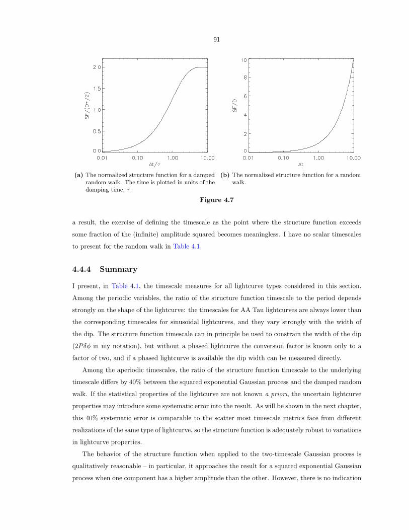
91

(a) The normalized structure function for a dampedrandom walk. The time is plotted in units of thedamping time, τ .

(b) The normalized structure function for a randomwalk.

Figure 4.7

a result, the exercise of defining the timescale as the point where the structure function exceeds

some fraction of the (infinite) amplitude squared becomes meaningless. I have no scalar timescales

to present for the random walk in Table 4.1.

4.4.4 Summary

I present, in Table 4.1, the timescale measures for all lightcurve types considered in this section.

Among the periodic variables, the ratio of the structure function timescale to the period depends

strongly on the shape of the lightcurve: the timescales for AA Tau lightcurves are always lower than

the corresponding timescales for sinusoidal lightcurves, and they vary strongly with the width of

the dip. The structure function timescale can in principle be used to constrain the width of the dip

(2Pδφ in my notation), but without a phased lightcurve the conversion factor is known only to a

factor of two, and if a phased lightcurve is available the dip width can be measured directly.

Among the aperiodic timescales, the ratio of the structure function timescale to the underlying

timescale differs by 40% between the squared exponential Gaussian process and the damped random

walk. If the statistical properties of the lightcurve are not known a priori, the uncertain lightcurve

properties may introduce some systematic error into the result. As will be shown in the next chapter,

this 40% systematic error is comparable to the scatter most timescale metrics face from different

realizations of the same type of lightcurve, so the structure function is adequately robust to variations

in lightcurve properties.

The behavior of the structure function when applied to the two-timescale Gaussian process is

qualitatively reasonable – in particular, it approaches the result for a squared exponential Gaussian

process when one component has a higher amplitude than the other. However, there is no indication

92

from the analysis that there is more than one component, or that the inferred timescale is effectively

a weighted average of the two real components. While the presence of two components could be

inferred from modeling the shape of the structure function (in particular, from features such as

the prominent “shoulder” in the middle row of Figure 4.6), such modeling would require making

assumptions about the lightcurve structure, contrary to the intent of the analysis presented here.

Model SF crosses 19

amp2 SF crosses 14

amp2 SF crosses 12

amp2

Sinusoid 0.154P 0.246P 0.450PAA Tau (10% Dip) 0.0425P = 0.85Pδφ Never NeverAA Tau (30% Dip) 0.0924P = 0.616Pδφ 0.170P = 1.133Pδφ NeverAA Tau (60% Dip) 0.127P = 0.423Pδφ 0.206P = 0.687Pδφ 0.359P = 1.197PδφWhite Noise 0 Never NeverSquared Exponential GP 1.356τ Never NeverTwo-Timescale GP (σ1 = 1

3σ2, τ1 = 1

10τ2) 12.759τ1 = 1.276τ2 Never Never

Two-Timescale GP (σ1 = 13σ2, τ1 = 1

3τ2) 3.828τ1 = 1.276τ2 Never Never

Two-Timescale GP (σ1 = σ2, τ1 = 110τ2) 6.726τ1 = 0.673τ2 Never Never

Two-Timescale GP (σ1 = σ2, τ1 = 13τ2) 2.354τ1 = 0.785τ2 Never Never

Two-Timescale GP (σ1 = 3σ2, τ1 = 110τ2) 1.483τ1 = 0.149τ2 Never Never

Two-Timescale GP (σ1 = 3σ2, τ1 = 13τ2) 1.460τ1 = 0.487τ2 Never Never

Damped Random Walk 0.919τ Never NeverRandom Walk Infinite Amplitude

Table 4.1: Trial scalar timescale measures, based on the structure function, for each of thelightcurve models introduced in section 4.2. Timescales are given in units of the period,P , for periodic sources and the characteristic timescale, τ , for aperiodic sources. For thetwo-timescale Gaussian process the results are expressed in terms of both the timescaleof the shorter component, τ1, and that of the longer component, τ2. For the AA Taulightcurve the results are expressed in terms of both the period, P , and the half-widthof the lightcurve’s periodic dip, Pδφ.

4.5 Autocovariance Functions

Having presented, in the previous section, the behavior of structure functions for each lightcurve

model introduced in section 4.2, in this section I calculate the ideal behavior of an autocovariance

function for the same set of models. The autocovariance function of a random signal M(t) is defined

as ACF (∆t) = E(M(t)M(t+∆t)), and can be seen as a measure of how well the magnitude at time

t predicts the magnitude at time t+ ∆t. Absolute values close to the variance V (M) mean that the

magnitude at t+ ∆t is tightly constrained.

The autocovariance can be related to the covariance function of M(t) by:

ACF (∆t) = E(M(t)M(t+ ∆t))

= cov (M(t),M(t+ ∆t)) + E(M(t))E(M(t+ ∆t)) (4.19)

If M(t) has constant mean, then

ACF (∆t) = cov (M(t),M(t+ ∆t)) + (E(M))2 (4.20)

93

The autocovariance function can also be related to the structure function by noting that both

depend on cov (M(t),M(t+ ∆t)):

ACF (∆t) = cov (M(t),M(t+ ∆t)) + E(M(t))E(M(t+ ∆t))

SF (∆t) = V (M(t))− (E(M(t)))2 − 2 cov (M(t),M(t+ ∆t)) + 2E(M(t))E(M(t+ ∆t))

+V (M(t+ ∆t))− (E(M(t+ ∆t)))2

ACF (∆t) = −1

2SF (∆t) +

1

2V (M(t))− 1

2(E(M(t)))2 + 2E(M(t))E(M(t+ ∆t))

+1

2V (M(t+ ∆t))− 1

2(E(M(t+ ∆t)))2 (4.21)

where I obtain the last expression by substituting for cov (M(t),M(t+ ∆t)). If M(t) has constant

mean, then

ACF (∆t) = −1

2SF (∆t) +

1

2V (M(t)) + E(M)2 +

1

2V (M(t+ ∆t)) (4.22)

If M(t) also has constant variance, then

ACF (∆t) = −1

2SF (∆t) + V (M) + E(M)2 (4.23)

Autocovariance has a growing presence in the literature, most often as a robust alternative to

periodograms (e.g., McQuillan et al., 2013). The most popular approach to autocovariances involves

taking bins of ∆t values (Edelson & Krolik, 1988), although some authors instead interpolate the

lightcurve to a regular grid (e.g., McQuillan et al., 2013). Note that many papers prefer the au-

tocorrelation function, ACF (∆t)/V (M), to the autocovariance function, and use ACF to denote

autocorrelation. The analysis of this section is expressed more simply in terms of the autocovari-

ance function, but my results for autocovariance can be converted into autocorrelation functions by

normalizing by ACF (0).

Autocovariance and autocorrelation functions of periodic sources tend to show a number of evenly

spaced peaks at integer multiples of the period; these peaks persist even in the presence of outliers

or systematic trends, which can introduce an overall slope in the ACF but do not create localized

artifacts (McQuillan et al., 2013).

For aperiodic sources the ACF typically shows a smooth downward trend from perfect correlation

at ∆t = 0 to values near zero. Many authors have adopted the first ∆t where the ACF equals zero as

a timescale measure (e.g., Abdo et al., 2010), arguing that it represents a transition from correlated

to anticorrelated behavior. As I show below, for many aperiodic sources, the ACF approaches zero

without crossing it, i.e., it shows a transition directly from correlated to uncorrelated behavior. In

such cases, the location of the zero crossing may instead be dominated by noise in the ACF. A more

subtle problem is that a nonzero mean in the lightcurve will introduce an offset in the ACF (note

94

the dependence on m0 in the examples that follow). While lightcurves are normally shifted to zero

mean before the ACF is calculated, any error in estimating the mean will produce a residual offset

that can create the appearance of correlated and anticorrelated regions in the ACF.

I evaluate converting an autocovariance function into a scalar timescale by finding the first

∆t at which the ACF crosses one ninth, one quarter, or one half of its value at zero time lag.

These values were selected on the basis of intuition: since the autocovariance has dimensions of

squared magnitudes, the first two thresholds correspond to variations of one third and one half the

lightcurve amplitude, respectively, while the last is midway between ACF(0) and a value of 0, which

for Gaussian process models represents a long-term asymptote (i.e., two signals measured a long

time apart are nearly uncorrelated).

As in the previous section, I first establish the behavior of the autocovariance function for a

sinusoidal signal, then for the other lightcurve models.

4.5.1 Sinusoid


ACF (∆t) = E(m(t)m(t+ ∆t))

=ω

2π

∫ t0+2π/ω

t0

(m0 +A sin (ω(t− t0))) (m0 +A sin (ω(t+ ∆t− t0))) dt

Let x = ω2π (t− t0) and let ∆x = ω

2π∆t. Then

ACF (∆t) =

∫ 1

0

(m0 +A sin 2πx) (m0 +A sin (2π(x+ ∆x))) dx

= m20 +

1

2A2 cos (2π∆x)

= m20 +

1

2A2 cos (ω∆t) (4.24)

The autocovariance function is shown in Figure 4.8a.

The scalar timescales calculated from the autocovariance function for a sine are listed in Table 4.2.

4.5.2 AA Tau

If

m(t) =


m0 otherwise

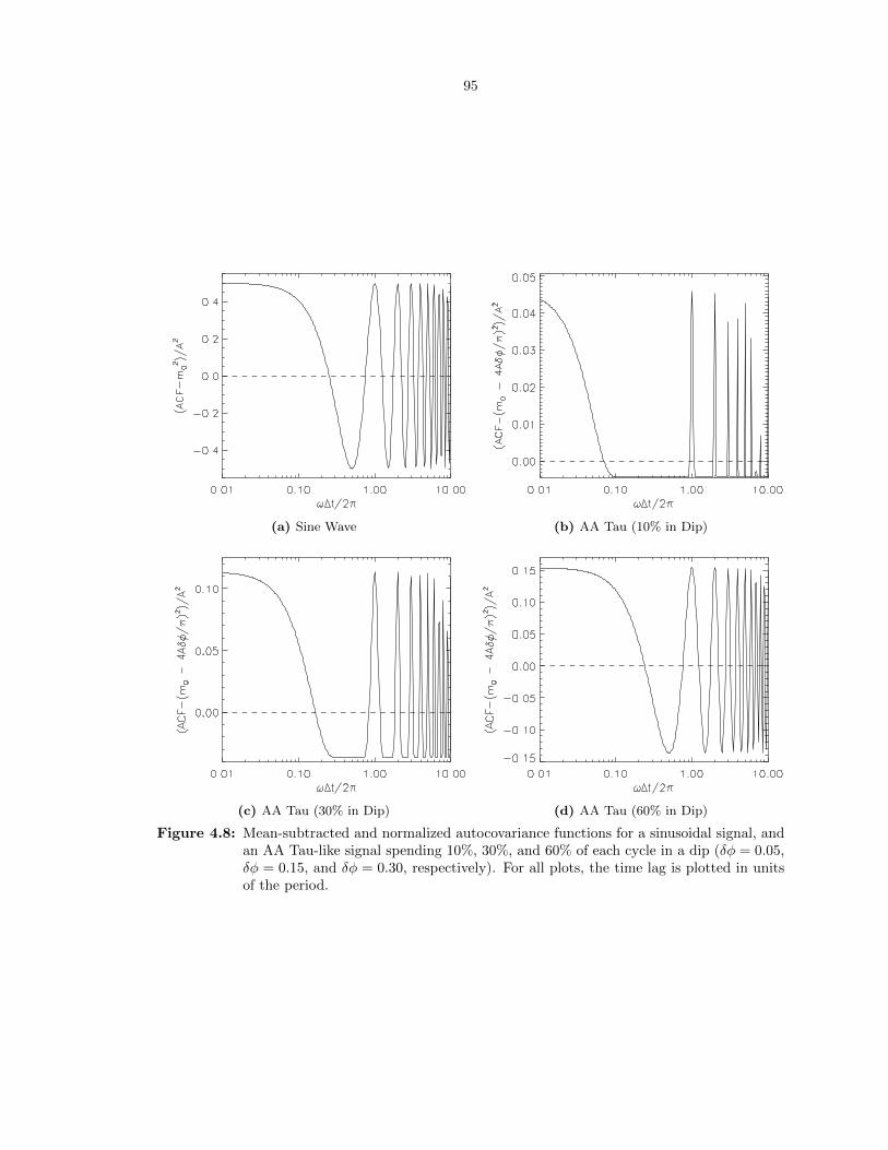
95

(a) Sine Wave (b) AA Tau (10% in Dip)

(c) AA Tau (30% in Dip) (d) AA Tau (60% in Dip)

Figure 4.8: Mean-subtracted and normalized autocovariance functions for a sinusoidal signal, andan AA Tau-like signal spending 10%, 30%, and 60% of each cycle in a dip (δφ = 0.05,δφ = 0.15, and δφ = 0.30, respectively). For all plots, the time lag is plotted in unitsof the period.

96

then the mean and variance of the signal are:

E(m) =

∫ 1/2

−1/2

m(φ)dφ

= m0 −4A

πδφ

V (m) =

∫ 1/2

−1/2

(m(φ)− E(m))2dφ

= A2δφ

(1− 16

π2δφ

)


ACF (∆t) = m20 −

8A

πm0δφ

−

A2

2π


(π∆φ2δφ

)− 2δφ sin

(π∆φ2δφ

))if ∆φ < 2δφ and ∆φ < 1− 2δφ

0 if ∆φ > 2δφ and ∆φ < 1− 2δφ

A2

2π


(π(1−∆φ)

2δφ

)− 2δφ sin

(π(1−∆φ)

2δφ

))if ∆φ > 2δφ and ∆φ > 1− 2δφ

A2

2π


(π(1−∆φ)

2δφ

)− 2δφ

(sin(π∆φ2δφ

)− sin

(π(1−∆φ−2δφ)

2δφ

))+ π(∆φ− 2δφ) cos

(π∆φ2δφ

))if ∆φ < 2δφ and ∆φ > 1− 2δφ

(4.25)

where ∆φ = frac( ω

2π∆t)

The autocovariance function is shown in Figure 4.8.

The scalar timescales calculated from the autocovariance function for an AA Tau are listed in

Table 4.2.


4.5.3.1 White Noise


ACF (∆t) =

σ2m +m2

0 if ∆t = 0

m20 if ∆t 6= 0

(4.26)


The ACF for a white noise process falls from ACF(0) to 0 at an infinitesimal value of ∆t, so the

timescale is effectively 0.

97

Figure 4.9: The mean-subtracted and normalized autocovariance function for a white noise process.The discontinuous value ACF (0)−m2

0 = σ2m is not shown.



ACF (∆t) = σ2me−(∆t)2/2τ2

+m20 (4.27)

The autocovariance function is shown in Figure 4.10a.

The scalar timescales calculated from the autocovariance function for a squared exponential

Gaussian process are listed in Table 4.2.



ACF (∆t) = σ21e−∆t2/2τ2

1 + σ22e−∆t2/2τ2

2 +m20 (4.28)


The scalar timescales calculated from the autocovariance function for a two-timescale Gaussian

process are listed in Table 4.2.



ACF (∆t) =Dτ

2e−|∆t|/τ +m2

0 (4.29)

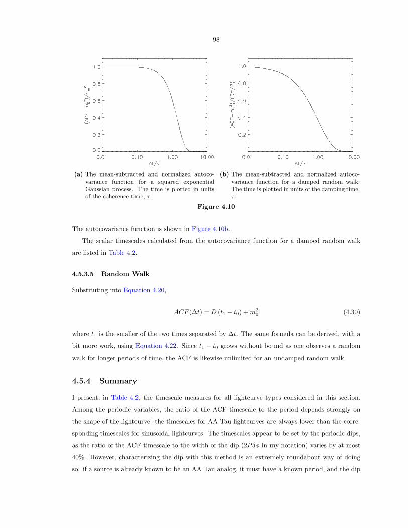
98

(a) The mean-subtracted and normalized autoco-variance function for a squared exponentialGaussian process. The time is plotted in unitsof the coherence time, τ .

(b) The mean-subtracted and normalized autoco-variance function for a damped random walk.The time is plotted in units of the damping time,τ .

Figure 4.10

The autocovariance function is shown in Figure 4.10b.

The scalar timescales calculated from the autocovariance function for a damped random walk

are listed in Table 4.2.

4.5.3.5 Random Walk


ACF (∆t) = D (t1 − t0) +m20 (4.30)

where t1 is the smaller of the two times separated by ∆t. The same formula can be derived, with a

bit more work, using Equation 4.22. Since t1 − t0 grows without bound as one observes a random

walk for longer periods of time, the ACF is likewise unlimited for an undamped random walk.

4.5.4 Summary


Among the periodic variables, the ratio of the ACF timescale to the period depends strongly on

the shape of the lightcurve: the timescales for AA Tau lightcurves are always lower than the corre-

sponding timescales for sinusoidal lightcurves. The timescales appear to be set by the periodic dips,

as the ratio of the ACF timescale to the width of the dip (2Pδφ in my notation) varies by at most

40%. However, characterizing the dip with this method is an extremely roundabout way of doing

so: if a source is already known to be an AA Tau analog, it must have a known period, and the dip

99

(a) σ1 = 13σ2, τ1 = 1

10τ2 (b) σ1 = 1

3σ2, τ1 = 1

3τ2

(c) σ1 = σ2, τ1 = 110τ2 (d) σ1 = σ2, τ1 = 1

3τ2

(e) σ1 = 3σ2, τ1 = 110τ2 (f) σ1 = 3σ2, τ1 = 1

3τ2

Figure 4.11: The mean-subtracted and normalized autocovariance function for a Gaussian processwith two incoherent variability components. Each panel adopts different assumptionsabout the relative amplitudes and timescales of the fast component (1) and the slowcomponent (2). The time is plotted in units of the coherence time for the slowercomponent, τ2.

100

width can be measured directly from the phased lightcurve.

Among the aperiodic timescales, the ratio of the ACF timescale to the underlying timescale

differs by 60% between the squared exponential Gaussian process and the damped random walk

if the time at which the ACF equals half its peak is taken as the timescale; it differs by at most

20% for the lower thresholds. If the statistical properties of the lightcurve are not known a priori,

the uncertain lightcurve properties may introduce some systematic error into the result. As will be

shown in the next chapter, the scatter most timescale metrics face from different realizations of the

same type of lightcurve is typically 40% or more, so a 20% systematic error is quite acceptable.

As for the structure function, the behavior of the ACF when applied to the two-timescale Gaus-

sian process has the expected asymptotic behaviors but gives no indication that there is more than

one component. Again, more detailed modeling, with specific assumptions about the lightcurve

structure, would be needed to separate the components.

Model ACF crosses 19

ACF crosses 14

ACF crosses 12

Sinusoid 0.232P 0.210P 0.167PAA Tau (10% Dip) 0.0597P = 1.194Pδφ 0.0505P = 1.010Pδφ 0.0371P = 0.742PδφAA Tau (30% Dip) 0.148P = 0.987Pδφ 0.129P = 0.860Pδφ 0.0979P = 0.653PδφAA Tau (60% Dip) 0.222P = 0.740Pδφ 0.198P = 0.660Pδφ 0.154P = 0.513PδφWhite Noise 0 0 0Squared Exponential GP 2.096τ 1.665τ 1.177τTwo-Timescale GP (σ1 = 1

3σ2, τ1 = 1

10τ2) 20.454τ1 = 2.045τ2 16.006τ1 = 1.601τ2 10.842τ1 = 1.084τ2


3τ2) 6.136τ1 = 2.045τ2 4.802τ1 = 1.601τ2 3.255τ1 = 1.085τ2

Two-Timescale GP (σ1 = σ2, τ1 = 110τ2) 17.344τ1 = 1.734τ2 11.774τ1 = 1.177τ2 2.607τ1 = 0.261τ2

Two-Timescale GP (σ1 = σ2, τ1 = 13τ2) 5.203τ1 = 1.734τ2 3.542τ1 = 1.181τ2 1.865τ1 = 0.622τ2

Two-Timescale GP (σ1 = 3σ2, τ1 = 110τ2) 2.859τ1 = 0.286τ2 1.887τ1 = 0.189τ2 1.272τ1 = 0.127τ2

Two-Timescale GP (σ1 = 3σ2, τ1 = 13τ2) 2.492τ1 = 0.831τ2 1.835τ1 = 0.612τ2 1.257τ1 = 0.419τ2

Damped Random Walk 2.197τ 1.386τ 0.693τRandom Walk ACF Undefined

Table 4.2: Trial scalar timescale measures, based on the autocovariance function, for each of thelightcurve models introduced in section 4.2. Timescales are given in units of the period,P , for periodic sources and the characteristic timescale, τ , for aperiodic sources. For thetwo-timescale Gaussian process the results are expressed in terms of both the timescaleof the shorter component, τ1, and that of the longer component, τ2. For the AA Taulightcurve the results are expressed in terms of both the period, P , and the half-widthof the lightcurve’s periodic dip, Pδφ.

4.6 ∆m-∆t Plots

In the previous two sections I studied structure functions and autocovariance functions, both well-

established tools for analyzing time series data. In this section I calculate the ideal behavior of a

new tool I developed, the ∆m-∆t plot, for each lightcurve model introduced in section 4.2.

The ∆m-∆t plot is a nonparametric representation of a lightcurve that describes the frequency

with which a particular degree of variability is observed on a particular timescale. In some ways

it resembles the self-correlation analysis of Percy et al. (2003, 2010), although it preserves more

information about the lightcurve’s behavior and thus allows a broader range of analysis techniques.

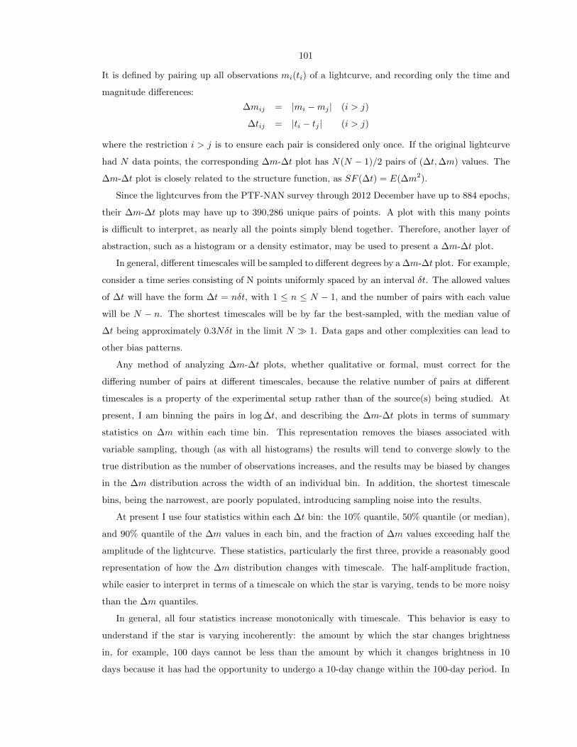
101

It is defined by pairing up all observations mi(ti) of a lightcurve, and recording only the time and

magnitude differences:

∆mij = |mi −mj | (i > j)

∆tij = |ti − tj | (i > j)

where the restriction i > j is to ensure each pair is considered only once. If the original lightcurve

had N data points, the corresponding ∆m-∆t plot has N(N − 1)/2 pairs of (∆t,∆m) values. The

∆m-∆t plot is closely related to the structure function, as SF (∆t) = E(∆m2).

Since the lightcurves from the PTF-NAN survey through 2012 December have up to 884 epochs,

their ∆m-∆t plots may have up to 390,286 unique pairs of points. A plot with this many points

is difficult to interpret, as nearly all the points simply blend together. Therefore, another layer of

abstraction, such as a histogram or a density estimator, may be used to present a ∆m-∆t plot.

In general, different timescales will be sampled to different degrees by a ∆m-∆t plot. For example,

consider a time series consisting of N points uniformly spaced by an interval δt. The allowed values

of ∆t will have the form ∆t = nδt, with 1 ≤ n ≤ N − 1, and the number of pairs with each value

will be N − n. The shortest timescales will be by far the best-sampled, with the median value of

∆t being approximately 0.3Nδt in the limit N 1. Data gaps and other complexities can lead to

other bias patterns.

Any method of analyzing ∆m-∆t plots, whether qualitative or formal, must correct for the

differing number of pairs at different timescales, because the relative number of pairs at different

timescales is a property of the experimental setup rather than of the source(s) being studied. At

present, I am binning the pairs in log ∆t, and describing the ∆m-∆t plots in terms of summary

statistics on ∆m within each time bin. This representation removes the biases associated with

variable sampling, though (as with all histograms) the results will tend to converge slowly to the

true distribution as the number of observations increases, and the results may be biased by changes

in the ∆m distribution across the width of an individual bin. In addition, the shortest timescale

bins, being the narrowest, are poorly populated, introducing sampling noise into the results.

At present I use four statistics within each ∆t bin: the 10% quantile, 50% quantile (or median),

and 90% quantile of the ∆m values in each bin, and the fraction of ∆m values exceeding half the

amplitude of the lightcurve. These statistics, particularly the first three, provide a reasonably good

representation of how the ∆m distribution changes with timescale. The half-amplitude fraction,

while easier to interpret in terms of a timescale on which the star is varying, tends to be more noisy

than the ∆m quantiles.

In general, all four statistics increase monotonically with timescale. This behavior is easy to

understand if the star is varying incoherently: the amount by which the star changes brightness

in, for example, 100 days cannot be less than the amount by which it changes brightness in 10

days because it has had the opportunity to undergo a 10-day change within the 100-day period. In

102

particular, if the star has no variability mechanisms operating on timescales longer than 10 days, then

the 100-day brightness change will simply be the (incoherent) sum of 10 10-day changes. A flattening

in the ∆m vs. ∆t curve therefore means that all the variability occurs on shorter timescales.

In the limits of infinite observing interval, infinite cadence, and noise-free measurements, the

discrete points of a ∆m-∆t plot merge into a continuous distribution: every timescale is sampled

an infinite number of times, and the density of pairs is given by a probability density function

f(∆m; ∆t). The Qth quantile of ∆m is the solution of F (∆m; ∆t) = Q for ∆m at fixed ∆t, where

F is the cumulative distribution function. The half-amplitude fraction is simply 1− F ( 12A; ∆t). To

allow a full range of analysis, for each trial lightcurve I find both f(∆m; ∆t) and F (∆m; ∆t).

I convert a ∆m-∆t plot into a scalar timescale by finding the first ∆t at which the median or

90% quantile crosses one third or one half of the amplitude. Both thresholds were chosen on the

basis of intuition: the median should represent the “typical” variability, and the 90% quantile the

“upper envelope,” while either one third or one half the total amplitude is a plausible definition of

significant variability. The high-amplitude fraction is redundant with the quantiles in this analysis:

the time at which Q of the pairs of ∆m values exceed F of the amplitude, where Q and F are

arbitrary fractions, is the time at which the (1−Q) quantile equals F of the amplitude.

As in the previous two sections, I first compute the ∆m-∆t plot for a simple sinusoidal signal,

then consider more complex lightcurve models.

4.6.1 Sinusoid


|∆m| = |A sin (ω(tj − t0))−A sin (ω(ti − t0))|

=

∣∣∣∣2A cos

(1

2ω(ti + tj − 2t0)

)sin

(1

2ω(tj − ti)

)∣∣∣∣Let xi = ω

2π (ti − t0) and let ∆x = xi − xj = ω2π∆t. Then

|∆m| = 2A| cos (π(xi + xj))|| sin (π∆x)|

= 2A| sin (π∆x)|| cos (π(2xi −∆x))|

If ∆t, and therefore ∆x, is held constant, the value of ∆m is determined entirely by the phase xi at

which one of the points is observed. The distribution function of ∆m is therefore

F (|∆m|; ∆t) = P (2A| sin (π∆x)|| cos (π(2xi −∆x))| ≤ |∆m|)

= P

(| cos (π(2xi −∆x))| ≤ |∆m|

2A| sin (π∆x)|

)

103

If |∆m|2A| sin (π∆x)| > 1, this probability is trivially 1. Otherwise, I note that | cos (π(2xi −∆x))| is

periodic with period 1, and that for continuous observations the phase of xi should be uniformly

distributed over the interval [0, 1). For convenience, I shift the phase convention, by a constant, to

the interval [ 12∆x− 1

2 ,12∆x+ 1

2 ). Then the probability becomes

P (| cos (π(2xi −∆x))| ≤ u; 0 ≤ u ≤ 1) =

∫ 12 ∆x+ 1

2

12 ∆x− 1

2

Θ(xi;u)f(xi)dxi

Θ(xi;u) =

1 if | cos (π(2xi −∆x))| ≤ u

0 otherwise

where f(xi) = 1 is the probability density function of xi. Changing variables,

P (| cos (π(2xi −∆x))| ≤ u) =

∫ 12

− 12

Θ(yi;u)f(yi)dyi

Θ(yi;u) =

1 if | cos (2πyi)| ≤ u

0 otherwise

This last integral is easy to evaluate:

P (| cos (π(2xi −∆x))| ≤ u) =

∫ − 1π cos−1 u

− 12

(1)f(yi)dyi +

∫ 1π cos−1 u

− 1π cos−1 u

(0)f(yi)dyi +

∫ 12

1π cos−1 u

(1)f(yi)dyi

= 1− 2

πcos−1 u

=2

πsin−1 u

Substituting for the dummy variable u,

F (|∆m|; ∆t) = P

(| cos (π(2xi −∆x))| ≤ |∆m|

2A| sin (π∆x)|

)

=

1 if 2A| sin ( 1

2ω∆t)| < |∆m|2π sin−1

(|∆m|

2A| sin ( 12ω∆t)|

)if 0 ≤ |∆m| ≤ 2A| sin ( 1

2ω∆t)|

0 if |∆m| < 0

(4.31)

Differentiating to get the probability density function,

f(|∆m|; ∆t) =

0 if 2A| sin ( 1

2ω∆t)| < |∆m|1

πA| sin ( 12ω∆t)|

1√1−(

|∆m|2A| sin ( 1

2ω∆t)|

)2if 0 ≤ |∆m| < 2A| sin ( 1

2ω∆t)|

0 if |∆m| < 0

(4.32)

104

Figure 4.12: Normalized ∆m-∆t plot for a sinusoidal signal. The left panel shows the densityfunction of ∆m as increasingly lighter shading, with 10th, 50th, and 90th percentilesof ∆m shown in red. The right panel shows the fraction of ∆m pairs exceeding halfthe amplitude. For both plots, ∆t is plotted in units of the period.

This density increases without bound as |∆m| approaches its maximum value 2A| sin ( 12ω∆t)|. The

distribution of ∆m as a function of ∆t is shown in Figure 4.12, as are the corresponding quantiles

and high-amplitude fractions.

The scalar timescales calculated from the ∆m-∆t plot for a sine are listed in Table 4.3.

4.6.2 AA Tau

If

m(t) =


m0 otherwise

then the signed magnitude difference ∆m can assume one of four forms:

∆m =

m0 −m0 if |φ| > δφ ∧ |φ+ ∆φ| > δφ

m0 −A cos(π2φδφ

)−m0 if |φ| < δφ ∧ |φ+ ∆φ| > δφ

m0 −m0 +A cos(π2φ+∆φδφ

)if |φ| > δφ ∧ |φ+ ∆φ| < δφ

m0 −A cos(π2φδφ

)−m0 +A cos

(π2φ+∆φδφ

)if |φ| < δφ ∧ |φ+ ∆φ| < δφ

depending on whether neither, either, or both the lightcurve at time t and time t+ ∆t are in a dip.

Here, ∆φ = frac(ω2π∆t

)− 1

2 ∈ [−1/2, 1/2) is the time lag in phase units, and it is implied that φ

and φ+ ∆φ are wrapped to stay in the interval [−1/2, 1/2) across the domain of each integral. Note

that the phase convention for ∆φ is different from that adopted in subsection 4.4.2, because I am

no longer looking at an explicit integration problem.

The probability distribution over these four cases cannot be directly treated using symbolic

105

mathematics packages such as Mathematica, because the combined logic of keeping the phases

straight and testing where the lightcurve is in or out of dip is too complex for them to handle. I

therefore evaluate each branch of the expression for ∆m separately, and then find the probability of

being in each case given ∆φ and ∆φ. The cumulative distribution function will then be given by

F (|∆m|; |∆t|) = F (|∆m|; |∆t| ∧ Case A)P (Case A; |∆t|)

+ F (|∆m|; |∆t| ∧ Case B)P (Case B; |∆t|)

+ F (|∆m|; |∆t| ∧ Case C)P (Case C; |∆t|)

+ F (|∆m|; |∆t| ∧ Case D)P (Case D; |∆t|)

(4.33)

and the probability density function will be given by an analogous decomposition.

4.6.2.1 Piecewise Probability Density and Distribution Functions

Case A |φ| > δφ ∧ |φ+ ∆φ| < δφ

In this case, ∆m is identically 0. In terms of probability distributions,

f(|∆m|; |∆t| ∧ Case A) = δ(∆m) (4.34)

F (|∆m|; |∆t| ∧ Case A) =

1 if |∆m| > 0

0 if |∆m| < 0(4.35)

where δ(x) denotes the Dirac delta function. Note that the cumulative distribution function F (|∆m|)

is undefined at zero.

Case B |φ| < δφ ∧ |φ+ ∆φ| > δφ

The magnitude difference is

|∆m| = A

∣∣∣∣cos

(π

2

φ

δφ

)∣∣∣∣= A| cos (πx)|

where x = φ2δφ ∈ [−1/2, 1/2] measures the position of phase φ relative to the dip. Since this case

assumes that φ + ∆φ is not in the dip, the allowed range of x depends on the value of ∆x = ∆φ2δφ .

Specifically,

x ∈

[−1/2, 1/2] if |∆x| > 1

[1/2−∆x, 1/2] if 0 < ∆x < 1

[−1/2,−1/2−∆x] if −1 < ∆x < 0

106

The cumulative distribution function for |∆m| is therefore

F (|∆m|; |∆t| ∧ Case B) = P (A|cos(πx)| ≤ |∆m|)

= P (|cos(πx)| ≤ |∆m|A

)

=

1 if |∆m|A > 1

1−∫ 1π cos−1 |∆m|/A− 1π cos−1 |∆m|/A dx if 0 < |∆m|

A < 1 ∧ |∆x| > 1

1− 1∆x

∫max 1π cos−1 |∆m|/A,1/2−∆x

max− 1π cos−1 |∆m|/A,1/2−∆x dx if 0 < |∆m|

A < 1 ∧ 0 < ∆x < 1

1− 1∆x

∫min 1π cos−1 |∆m|/A,−1/2−∆x

min− 1π cos−1 |∆m|/A,−1/2−∆x dx if 0 < |∆m|

A < 1 ∧ −1 < ∆x < 0

0 if |∆m|A < 0

Note that for sufficiently large |∆x| the integrals may be over an interval of zero length. This

happens when x is forced to be near the edges of the dip, and | cos(πx)| ≤ |∆m|A for all allowed x.

Since the integrands are trivial and only the limits depend on ∆x, the above equation may be

integrated on a case-by-case basis to give

F (|∆m|; |∆t| ∧ Case B) =

1 if |∆m|A > 1

1− 2π cos−1

(|∆m|A

)if |∆m|A < 1 ∧ |∆x| > 1

1− 2π|∆x| cos−1

(|∆m|A

)if sin(π|∆x|) < |∆m|

A < 1 ∧ 1/2 < |∆x| < 1

1 if sin(π|∆x|) < |∆m|A < 1 ∧ 0 < |∆x| < 1/2

1− 1|∆x|

(1π cos−1

(|∆m|A

)+ |∆x| − 1/2

)if 0 < |∆m|

A < sin(π|∆x|) ∧ |∆x| < 1

0 if |∆m|A < 0

(4.36)

Differentiating to get the density function,

f(|∆m|; |∆t| ∧ Case B) =

0 if |∆m|A > 1

2πA

1√1−( |∆m|A )

2if |∆m|A < 1 ∧ |∆x| > 1

2πA|∆x|

1√1−( |∆m|A )

2if sin(π|∆x|) < |∆m|

A < 1 ∧ 1/2 < |∆x| < 1

0 if sin(π|∆x|) < |∆m|A < 1 ∧ 0 < |∆x| < 1/2

1πA|∆x|

1√1−( |∆m|A )

2if 0 < |∆m|

A < sin(π|∆x|) ∧ |∆x| < 1

0 if |∆m|A < 0

(4.37)

Case C |φ| > δφ ∧ |φ+ ∆φ| < δφ

Since this case is Case B with φ and (φ + ∆φ) interchanged, the solution is the same as for

Case B.

107

Case D |φ| < δφ ∧ |φ+ ∆φ| < δφ

The magnitude difference is

|∆m| =

∣∣∣∣A cos

(π

2

φ

δφ

)−A cos

(π

2

φ+ ∆φ

δφ

)∣∣∣∣= 2A

∣∣∣∣sin(π4 2φ+ ∆φ

δφ

)∣∣∣∣ ∣∣∣∣sin(π4 ∆φ

δφ

)∣∣∣∣= 2A

∣∣∣sin(π2

(2x+ ∆x))∣∣∣ ∣∣∣sin(π

2∆x)∣∣∣

where, as before, x = φ2δφ ∈ [−1/2, 1/2] and ∆x = ∆φ

2δφ . The values of x allowed by the constraint

that both x and x+ ∆x fall in the dip are

x ∈

[∆x− 1/2, 1/2] if 0 < ∆x < 1

[−1/2,∆x+ 1/2] if −1 < ∆x < 0

The case |∆x| > 1 is incompatible with the assumption that both x and x+ ∆x are in the dip, since

the dip has width 1 in the units of x and ∆x.

It follows that the expression 12 (2x + ∆x) that appears in the expression for |∆m| falls in the

range

1

2(2x+ ∆x) ∈

[ 12∆x− 1

2 ,12 −

12∆x] if 0 < ∆x < 1

[− 12 −

12∆x, 1

2∆x+ 12 ] if −1 < ∆x < 0

The cumulative distribution function for |∆m| is therefore

F (|∆m|; |∆t| ∧ Case D) = P(

2A∣∣∣sin(π

2(2x+ ∆x)

)∣∣∣ ∣∣∣sin(π2

∆x)∣∣∣ ≤ |∆m|)

= P

(∣∣∣sin(π2

(2x+ ∆x))∣∣∣ ≤ |∆m|

2A∣∣sin (π2 ∆x

)∣∣)

= P (|sin (πy)|) ≤ u

=

1

1−∆x

∫min 1π sin−1 u, 12−

12 ∆x

max− 1π sin−1 u, 12 ∆x− 1

2dy if 0 < ∆x < 1

11+∆x

∫min 1π sin−1 u, 12−

12 ∆x

max− 1π sin−1 u,− 1

2 ∆x− 12dy if −1 < ∆x < 0

Since the integrands are trivial and only the limits depend on ∆x, the above equation may be

integrated on a case-by-case basis to give

F (|∆m|; |∆t| ∧ Case D) =

1 if |∆m|

2A|sin (π2 ∆x)| > sin(π2 −

π2 |∆x|

)2

π(1−|∆x|) sin−1

(|∆m|

2A|sin (π2 ∆x)|

)if 0 < |∆m|

2A|sin (π2 ∆x)| < sin(π2 −

π2 |∆x|

)0 if |∆m|

2A|sin (π2 ∆x)| < 0

(4.38)

108

Differentiating to get the density function,

f(|∆m|; |∆t| ∧ Case D) =

0 if |∆m|2A|sin (π2 ∆x)| > sin

(π2 −

π2 |∆x|

)1

π(1−|∆x|)A|sin (π2 ∆x)|1√√√√1−

(|∆m|

2A|sin (π2 ∆x)|

)2if 0 < |∆m|

2A|sin (π2 ∆x)| < sin(π2 −

π2 |∆x|

)0 if |∆m|

2A|sin (π2 ∆x)| < 0

(4.39)

4.6.2.2 Probabilities of the Cases

In general, the probabilities of the four cases in Equation 4.33 depend on the values of δφ, the

half-width of the dip, and ∆φ, the time lag. For a given lightcurve shape, i.e., a fixed δφ, there are

six values of ∆φ where the probabilities may change discontinuously:

• if |∆φ| = 2δφ, then when one of m(φ) and m(φ + ∆φ) is at the beginning of a dip the other

will be at the end. For smaller values of ∆φ it is possible for m(φ) and m(φ+ ∆φ) to both be

in the same dip at the same value of φ, while for larger values it is not.

• if |∆φ| = 1 − 2δφ, then when one of m(φ) and m(φ + ∆φ) is at the end of a dip the other

will be at the beginning of the next dip. For larger values of ∆φ it is possible for m(φ) and

m(φ+ ∆φ) to both be in a dip at the same value of φ, while for smaller values it is not.

• if |∆φ| = 1/2 − δφ, then when one of m(φ) and (φ + ∆φ) is at the end of a dip the other

reaches ±1/2 and needs to be wrapped around. For larger ∆φ the wraparound occurs while

one function is in the dip, while for smaller ∆φ the wraparound occurs while neither function

is in a dip. The complementary case, |∆φ| = 1/2 + δφ, does not occur for ∆φ ∈ [−1/2, 1/2).

These six critical values of ∆φ divide the parameter space into five different cases, as illustrated in

Figure 4.13a.

Case I |∆φ| < 2δφ ∧ |∆φ| < 1/2− δφ

This situation is shown in Figure 4.13b, where the diagonal line — the set of allowed combinations

of φ and φ + ∆φ — can find itself in any of the four cases A-D. Noting that the intercept of the

109

(a) All Cases (b) Case I

(c) Case II (d) Case III

(e) Case IV (f) Case V

Figure 4.13: a): the five cases described in subsubsection 4.6.2.2, plotted as a function of thedip half-width δφ and the time lag in phase units ∆φ. Colors highlight the regionswhere each of the branches of Equation 4.33 holds. Other panels: plots of the allowedcombinations of φ and φ + ∆φ over the course of a full period. Dashed lines are at±δφ, and divide cases A, B, C, and D (see subsubsection 4.6.2.1) from each other.

110

diagonal line is ∆φ, the fraction of phases spent in each case is:

P (Case A; |∆t|) = 1− 2δφ−∆φ

P (Case B; |∆t|) = ∆φ

P (Case C; |∆t|) = ∆φ

P (Case D; |∆t|) = 2δφ−∆φ

Call these probabilities “Solution A.”

Case II |∆φ| < 2δφ ∧ 1/2− δφ < |∆φ| < 1− 2δφ

This situation, shown in Figure 4.13c, differs from Case I only in the location of the phase

wraparound relative to the boundaries between Cases A, B, and C. The fraction of phases spent in

each case is:

P (Case A; |∆t|) = 1− 2δφ−∆φ

P (Case B; |∆t|) = ∆φ

P (Case C; |∆t|) = ∆φ

P (Case D; |∆t|) = 2δφ−∆φ

These are also Solution A.

Case III |∆φ| < 2δφ ∧ 1− 2δφ < |∆φ|

In this case, shown in Figure 4.13d, the spacing ∆φ between the two observations is larger than

the amount of time between the end of one dip and the beginning of the next. Therefore, Case A is

impossible. From the plot, the probabilities can be seen to be

P (Case A; |∆t|) = 0

P (Case B; |∆t|) = 1− 2δφ

P (Case C; |∆t|) = 1− 2δφ

P (Case D; |∆t|) = 4δφ− 1

Call these probabilities “Solution B.”

111

Case IV |∆φ| > 2δφ ∧ |∆φ| < 1/2− δφ

In this case, shown in Figure 4.13d, the spacing ∆φ between the two observations is larger than

the width of the dip. Therefore, Case D is impossible. From the plot, the probabilities can be seen

to be

P (Case A; |∆t|) = 1− 4δφ

P (Case B; |∆t|) = 2δφ

P (Case C; |∆t|) = 2δφ

P (Case D; |∆t|) = 0

Call these probabilities “Solution C.”

Case V |∆φ| > 2δφ ∧ 1/2− δφ < |∆φ| < 1− 2δφ

This situation, shown in Figure 4.13c, differs from Case IV only in the location of the phase

wraparound relative to the boundaries between Cases A, B, and C. The fraction of phases spent in

each case is:

P (Case A; |∆t|) = 1− 4δφ

P (Case B; |∆t|) = 2δφ

P (Case C; |∆t|) = 2δφ

P (Case D; |∆t|) = 0

These are also Solution C.

Equation 4.33 may now be used to find F (|∆m|) and f(|∆m|) for any value of ∆φ = frac(ω2π∆t

)−

12 . The resulting expressions are evaluated in Figure 4.14.

The scalar timescales calculated from the ∆m-∆t plot for an AA Tau-like lightcurve are listed

in Table 4.3.


By definition, the magnitude measurements M(t) sampled from a Gaussian process are jointly

normally distributed random variables. Therefore, their signed difference ∆m is itself a normal

112

(a) 10% in Dip (b) 10% in Dip

(c) 30% in Dip (d) 30% in Dip

(e) 60% in Dip (f) 60% in Dip

Figure 4.14: Normalized ∆m-∆t plots for an AA Tau-like signal spending 10%, 30%, and 60% ofeach cycle in a dip (δφ = 0.05, δφ = 0.15, and δφ = 0.30, respectively). The left panelshows the density function of ∆m as increasingly lighter shading, with 10th, 50th,and 90th percentiles of ∆m shown in red. Note that the 10th and 50th percentilesare often zero, reflecting the large number of pairs of points where both observationsin the pair were taken outside a dip. The right panel shows the fraction of ∆m pairsexceeding half the amplitude. For all plots, ∆t is plotted in units of the period.

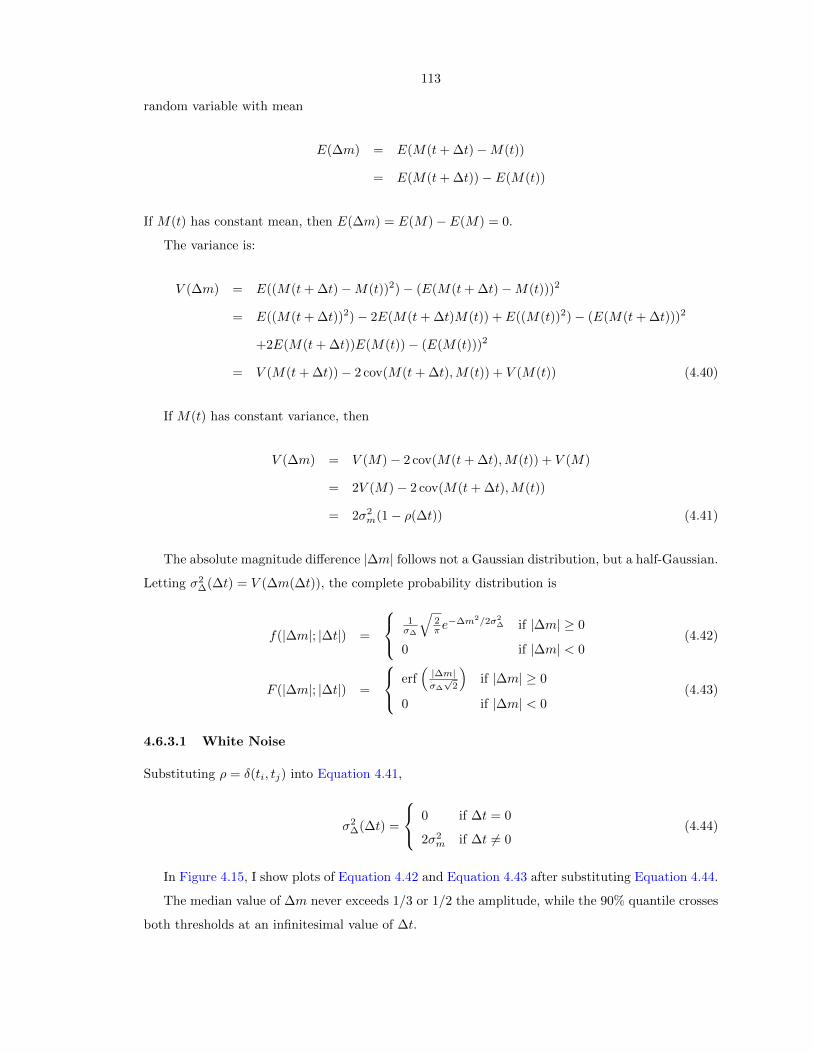
113

random variable with mean

E(∆m) = E(M(t+ ∆t)−M(t))

= E(M(t+ ∆t))− E(M(t))

If M(t) has constant mean, then E(∆m) = E(M)− E(M) = 0.

The variance is:

V (∆m) = E((M(t+ ∆t)−M(t))2)− (E(M(t+ ∆t)−M(t)))2

= E((M(t+ ∆t))2)− 2E(M(t+ ∆t)M(t)) + E((M(t))2)− (E(M(t+ ∆t)))2

+2E(M(t+ ∆t))E(M(t))− (E(M(t)))2

= V (M(t+ ∆t))− 2 cov(M(t+ ∆t),M(t)) + V (M(t)) (4.40)

If M(t) has constant variance, then

V (∆m) = V (M)− 2 cov(M(t+ ∆t),M(t)) + V (M)

= 2V (M)− 2 cov(M(t+ ∆t),M(t))

= 2σ2m(1− ρ(∆t)) (4.41)

The absolute magnitude difference |∆m| follows not a Gaussian distribution, but a half-Gaussian.

Letting σ2∆(∆t) = V (∆m(∆t)), the complete probability distribution is

f(|∆m|; |∆t|) =

1σ∆

√2π e−∆m2/2σ2

∆ if |∆m| ≥ 0

0 if |∆m| < 0(4.42)

F (|∆m|; |∆t|) =

erf(|∆m|σ∆

√2

)if |∆m| ≥ 0

0 if |∆m| < 0(4.43)

4.6.3.1 White Noise

Substituting ρ = δ(ti, tj) into Equation 4.41,

σ2∆(∆t) =

0 if ∆t = 0

2σ2m if ∆t 6= 0

(4.44)

In Figure 4.15, I show plots of Equation 4.42 and Equation 4.43 after substituting Equation 4.44.

The median value of ∆m never exceeds 1/3 or 1/2 the amplitude, while the 90% quantile crosses

both thresholds at an infinitesimal value of ∆t.

114

Figure 4.15: Normalized ∆m-∆t plot for a white noise process. The left panel shows the densityfunction of ∆m as increasingly lighter shading, with quantiles of ∆m shown in red.The discontinuity at ∆t = 0 is not shown. The right panel shows the fraction of ∆mpairs exceeding half the amplitude.


Substituting ρ = e−∆t2/2τ2

into Equation 4.41,

σ2∆(∆t) = 2σ2

m

(1− e−∆t2/2τ2

)(4.45)

The corresponding plots are shown in Figure 4.16. The scalar timescales calculated from the

∆m-∆t plot for a squared exponential Gaussian process are listed in Table 4.3.


The variance in Equation 4.5 is easiest to use with Equation 4.40:

σ2∆(∆t) = σ2

1 + σ22 − 2σ2

1e−∆t2/2τ2

1 + σ22e−∆t2/2τ2

2 + σ21 + σ2

2

= 2(σ21 + σ2

2)− 2σ21e−∆t2/2τ2

1 − 2σ22e−∆t2/2τ2

2 (4.46)

The corresponding plots are shown in Figures 4.17 and 4.18, for different regimes of σ1/σ2 and

τ1/τ2.

The scalar timescales calculated from the ∆m-∆t plot for a two-timescale Gaussian process are

listed in Table 4.3.

115

Figure 4.16: Normalized ∆m-∆t plot for a squared exponential Gaussian process. The left panelshows the density function of ∆m as increasingly lighter shading, with quantiles of∆m shown in red. The right panel shows the fraction of ∆m pairs exceeding half theamplitude. For both plots, ∆t is plotted in units of the correlation time.


Substituting ρ = e−|ti−tj |/τ into Equation 4.41,

σ2∆(∆t) = Dτ

(1− e−|∆t|/τ

)(4.47)

The corresponding distribution is shown in Figure 4.19. The scalar timescales calculated from

the ∆m-∆t plot for a damped random walk are listed in Table 4.3.

4.6.3.5 Random Walk

Substituting the formulas in Equations 4.7 and Equation 4.8 into Equation 4.40 (note that, since

the variance is not constant, Equation 4.41 does not apply),

σ2∆(∆t) = D(ti − t0)− 2D(t1 − t0) +D(tj − t0)

=

D(ti − t0)− 2D(ti − t0) +D(tj − t0) if ti < tj

D(ti − t0)− 2D(tj − t0) +D(tj − t0) if ti > tj

=

D(tj − ti) if ti < tj

D(ti − tj) if ti > tj

= D|∆t| (4.48)

While both the variance and the covariance of a random walk depend on the starting time t0, the

distribution of ∆m as a function of ∆t does not. The distribution is shown in Figure 4.20.

116

(a) σ1 = 13σ2, τ1 = 1

10τ2 (b) σ1 = 1

3σ2, τ1 = 1

3τ2

(c) σ1 = σ2, τ1 = 110τ2 (d) σ1 = σ2, τ1 = 1

3τ2

(e) σ1 = 3σ2, τ1 = 110τ2 (f) σ1 = 3σ2, τ1 = 1

3τ2

Figure 4.17: Normalized ∆m-∆t plot for a two-timescale Gaussian process. The density functionof ∆m is indicated by increasingly lighter shading, with quantiles of ∆m shown in red.Each panel adopts different assumptions about the relative amplitudes and timescalesof the fast component (1) and the slow component (2). The time is plotted in unitsof the coherence time for the slower component, τ2.

117

(a) σ1 = 13σ2, τ1 = 1

10τ2 (b) σ1 = 1

3σ2, τ1 = 1

3τ2

(c) σ1 = σ2, τ1 = 110τ2 (d) σ1 = σ2, τ1 = 1

3τ2

(e) σ1 = 3σ2, τ1 = 110τ2 (f) σ1 = 3σ2, τ1 = 1

3τ2

Figure 4.18: Fraction of ∆m pairs exceeding half the amplitude for a two-timescale Gaussianprocess. Each panel adopts different assumptions about the relative amplitudes andtimescales of the fast component (1) and the slow component (2). The time is plottedin units of the coherence time for the slower component, τ2.

118

Figure 4.19: Normalized ∆m-∆t plot for a damped random walk. The left panel shows the densityfunction of ∆m as increasingly lighter shading, with quantiles of ∆m shown in red.The right panel shows the fraction of ∆m pairs exceeding half the amplitude. Forboth plots, ∆t is plotted in units of the damping time.

While the ∆m-∆t plot is well defined, the lightcurve amplitude is not, so there is no way to set

a threshold for the ∆m-∆t quantiles to cross. There is therefore no timescale associated with the

∆m-∆t analysis.

4.6.4 Summary


Among the periodic variables, the ratio of the structure function timescale to the period depends

strongly on the shape of the lightcurve: the timescales for AA Tau lightcurves are always lower than

the corresponding timescales for sinusoidal lightcurves, and they vary strongly with the width of

the dip. However, the timescale is not proportional to the width of the dip, and cannot be used to

characterize it.

Among the aperiodic timescales, the ratio of the ∆m-∆t timescale to the underlying timescale

differs by a factor of two to three between the squared exponential Gaussian process and the damped

random walk. If the statistical properties of the lightcurve are not known a priori, the uncertain

lightcurve properties may introduce a systematic error of a factor of two or more into the result.

As with the structure function and the autocovariance function, the behavior of ∆m-∆t plots

when applied to the two-timescale Gaussian process has the expected asymptotic behaviors but gives

no indication that there is more than one component. Again, more detailed modeling, with specific

assumptions about the lightcurve structure, would be needed to separate the components.

119

Figure 4.20: Normalized ∆m-∆t plot for a random walk. The density function of ∆m is indicatedby increasingly lighter shading, with quantiles of ∆m shown in red.

Median crosses Median crosses 90% quantile crosses 90% quantile crossesModel 1

3 amp 12 amp 1

3 amp 12 amp

Sinusoid 0.154P 0.246P 0.108P 0.167PAA Tau (10% Dip) Never Never 0.0312P = 0.624Pδφ 0.0417P = 0.834PδφAA Tau (30% Dip) Never Never 0.0388P = 0.257Pδφ 0.0616P = 0.411PδφAA Tau (60% Dip) 0.175P = 0.583Pδφ 0.255P = 0.850Pδφ 0.0694P = 0.231Pδφ 0.109P = 0.363PδφWhite Noise Never Never 0 0Squared Exponential GP Never Never 0.709τ 1.178τTwo-Timescale GP (σ1 = 1

3σ2, τ1 = 110 τ2) Never Never 5.403τ1 = 0.540τ2 10.842τ1 = 1.084τ2


3 τ2) Never Never 1.766τ1 = 0.589τ2 3.255τ1 = 1.085τ2Two-Timescale GP (σ1 = σ2, τ1 = 1

10 τ2) Never Never 1.075τ1 = 0.107τ2 2.607τ1 = 0.261τ2Two-Timescale GP (σ1 = σ2, τ1 = 1

3 τ2) Never Never 0.996τ1 = 0.332τ2 1.865τ1 = 0.622τ2Two-Timescale GP (σ1 = 3σ2, τ1 = 1

10 τ2) Never Never 0.753τ1 = 0.0753τ2 1.272τ1 = 0.127τ2Two-Timescale GP (σ1 = 3σ2, τ1 = 1

3 τ2) Never Never 0.747τ1 = 0.249τ2 1.257τ1 = 0.419τ2Damped Random Walk Never Never 0.251τ 0.693τRandom Walk Infinite Amplitude

Table 4.3: Trial scalar timescale measures, based on the ∆m-∆t plot, for each of the lightcurvemodels introduced in section 4.2. Timescales are given in units of the period, P , forperiodic sources and the characteristic timescale, τ , for aperiodic sources. For the two-timescale Gaussian process the results are expressed in terms of both the timescale ofthe shorter component, τ1, and that of the longer component, τ2. For the AA Taulightcurve the results are expressed in terms of both the period, P , and the half-widthof the lightcurve’s periodic dip, Pδφ.

4.7 Summary of Theoretical Results

In this chapter I’ve tested, under highly idealized conditions, three candidate timescale metrics

(structure functions, autocovariance functions, and ∆m-∆t plots) on six types of lightcurve models:

a sine, a periodic “dipper” like AA Tau, a squared exponential Gaussian process, a variant of the

squared exponential Gaussian process having two components with different timescales, a damped

random walk, and an (undamped) random walk. By testing each timescale metric on a variety of

lightcurve models, I was able to determine how well each metric adapts to different lightcurves and

also ensure that the analysis was not biased by a single model on which a particular metric performs

unusually well or poorly. To my knowledge, this is the first such analysis of timescale metrics,

and in particular the first to attempt to characterize performance without reference to an assumed

120

lightcurve model.

Criterion Structure Function Autocovariance Function ∆m-∆t PlotUniversal Yes Yes YesData-driven May require binning/interpolation May require binning/interpolation May require binningVersatile to ∼ 40% to ∼ 20% to factor of 2Accurate Yes Yes Yes

Table 4.4: Performance of three candidate timescale metrics with respect to the criteria introducedin section 4.1. An entry beginning with “May require” means that, while the timescalemetric itself satisfies the criterion, a specific algorithm for calculating the metric maynot.

The performance of each metric across the various lightcurves was described in detail in sec-

tions 4.4 through 4.6. A summary of the results, in terms of the criteria introduced in section 4.1, is

presented in Table 4.4. All three metrics are universal, by construction. They are likewise accurate

except when applied to the two lightcurve models that had more parameters than a single timescale,

namely AA Tau lightcurves and two-timescale Gaussian processes. This behavior appears to be a

problem with the models, rather than with the timescale metrics: the concept of “the timescale

of the lightcurve” is ill-defined in the context of either model. As a result, neither model will be

considered further.

The three metrics differ primarily by how well they handle a variety of lightcurves, particularly

the aperiodic lightcurves for which the metrics are intended. Autocovariance functions are the

most reliable by this criterion, with variation in the lightcurve function affecting the conversion to

underlying timescale by only 20%. ∆m-∆t plots are most affected by changes to the statistical

properties of the lightcurve; the additional small-scale structure in a damped random walk produces

an estimated timescale at most half that for a squared exponential Gaussian process with the same

characteristic timescale. This is a significant limitation to ∆m-∆t plots compared to the other two

metrics.

Autocovariance functions and ∆m-∆t plots are tested further in the next chapter, using numerical

simulations. Due to time constraints, I was unable to test an implementation of a structure function

on simulated data.

121

4.8 References

Abdo, A. A. et al. 2010, ApJ, 722, 520, arXiv:1004.0348

Doob, J. L. 1942, Annals of Mathematics, 43, 351

Edelson, R. A., & Krolik, J. H. 1988, ApJ, 333, 646

Gillespie, D. T. 1996, American Journal of Physics, 64, 225

Lenz, P., & Breger, M. 2005, Communications in Asteroseismology, 146, 53

Lomb, N. R. 1976, Ap&SS, 39, 447

McQuillan, A., Aigrain, S., & Mazeh, T. 2013, MNRAS, 432, 1203, arXiv:1303.6787

Paltani, S., Courvoisier, T. J.-L., Blecha, A., & Bratschi, P. 1997, A&A, 327, 539, astro-ph/9706203

Percy, J. R., Grynko, S., Seneviratne, R., & Herbst, W. 2010, PASP, 122, 753

Percy, J. R., Hosick, J., & Leigh, N. W. C. 2003, PASP, 115, 59

Scargle, J. D. 1982, ApJ, 263, 835

Simonetti, J. H., Cordes, J. M., & Heeschen, D. S. 1985, ApJ, 296, 46

122

Chapter 5

Numerical Performance ofTimescale Metrics

5.1 Introduction

This chapter continues the search for a practical aperiodic timescale definition started in Chapter 4.

There, I defined a good aperiodic timescale metric as one that is:

Universal: it is defined for any lightcurve with any sampling, provided some minimum number of

data points are present. In particular, it should not require evenly spaced samples, nor should

it place preconditions on the properties of the underlying signal.

Data-Driven: it does not require hand-tuning, but is determined entirely by the data.

Versatile: it gives consistent results across lightcurves having different shapes or characteristic

behaviors

Accurate: it correlates with the “true” timescale of a lightcurve

Precise: it has a low statistical variance

Dependable: it gives consistent results across different noise levels or cadences

Robust: it changes little if a small number of data points are added or removed, even if those points

are outliers

Well-Characterized: it offers a way to determine the significance of the detected timescale

The definition of a timescale metric determines whether it is universal or data driven, so these

criteria do not require testing. The previous chapter derived analytical expressions for timescale

metrics as applied in the hypothetical case of perfect knowledge of the lightcurve, allowing me

to rank timescale metrics based on their versatility and, to a lesser degree, their accuracy. The

remaining criteria cannot be evaluated without realistic, or, in other words, imperfect, test data.

123

To determine the impact of measurement noise, limited cadence, and finite observing windows

on lightcurve analysis, I simulated observations of the family of signals defined in section 4.2 at

several key cadences. By determining how the precision and accuracy of timescale estimates depend

on noise, cadence, and outliers, I can evaluate how each timescale metric performs by the above

criteria. This is the first systematic attempt to use simulations to identify the best timescale metric

for aperiodic lightcurves.

5.1.1 LightcurveMC: an extensible lightcurve simulation program

I have developed a program to generate random lightcurves and to perform automated statistical

analysis of each lightcurve. LightcurveMC is designed to be highly modular, allowing new lightcurve

types or new analysis tools to be introduced without excessive development overhead. The statistical

tools are completely agnostic to how the lightcurve data is generated, and the lightcurve generators

are completely agnostic to how the data will be analyzed. The use of fixed random seeds throughout

guarantees that the program generates consistent results from run to run.

All figures and results in this chapter were generated using LightcurveMC 2.3.0. It is available,

with documentation, from the Astrophysics Source Code Library as ascl:1408.012 (Findeisen, 2014).

For the simulation runs presented here, the program was built using GCC 4.4.7-3 on Red Hat

Enterprise Linux 6.4 and linked against kpfutils1 1.0.0, Timescales2 1.0.0, Boost3 1.41.0, GSL4 1.10,

TCLAP5 1.2.1, R6 2.15.1, Rcpp7 0.10.3, RInside8 0.2.10, gptk9 1.06, and numDeriv10 2012.9-1. The

random generation of squared exponential and two-timescale Gaussian processes is sensitive to the

version of GSL, but otherwise the program output reported here should be reproducible regardless

of compiler, interpreter, or library version.

5.1.2 Input Cadences

I tested timescale metrics on four observing cadences, representing different young star monitoring

programs recently carried out at Caltech and the Infrared Processing and Analysis Facility. The

cadences, presented in Table 5.1, were selected to probe different observing regimes. The PTF-NAN

Full cadence is the cadence at which we observed the North America Nebula with the Palomar

Transient Factory from 2009 August to 2012 December. The PTF-NAN 2010 cadence is the subset

of these observations that were taken in 2010. The YSOVAR 2010 cadence represents a month

1https://github.com/kfindeisen/kpfutils2https://github.com/kfindeisen/Timescales3http://www.boost.org/4http://www.gnu.org/software/gsl/5http://tclap.sourceforge.net/6http://www.r-project.org/7http://dirk.eddelbuettel.com/code/rcpp.html8http://dirk.eddelbuettel.com/code/rinside.html9http://cran.r-project.org/web/packages/gptk/

10http://cran.r-project.org/web/packages/numDeriv/

https://github.com/kfindeisen/kpfutils

https://github.com/kfindeisen/Timescales

http://www.boost.org/

http://www.gnu.org/software/gsl/

http://tclap.sourceforge.net/

http://www.r-project.org/

http://dirk.eddelbuettel.com/code/rcpp.html

http://dirk.eddelbuettel.com/code/rinside.html

http://cran.r-project.org/web/packages/gptk/

http://cran.r-project.org/web/packages/numDeriv/

124

of Spitzer observations for the Young Stellar Object Variability survey (Morales-Calderon et al.,

2011) to represent a higher-cadence and shorter-baseline monitoring program than either of the two

PTF-NAN cadences. Finally, the CoRoT cadence represents a month of high-frequency observations

taken by Cody et al. (2014) to probe the extremes of both very high cadence and very large number

of points.

Cadence Size Baseline Char. Cadence Median Gap Longest Gap Regularity(days) (days) (days) (days)

PTF-NAN Full 910 1,224.9 0.21 0.048 179.3 0.811PTF-NAN 2010 126 252.7 1.98 0.91 17.0 0.973YSOVAR 2010 39 35.7 1.26 0.91 2.5 0.954CoRoT 6,307 38.7 0.012 0.0059 0.78 0.997

Table 5.1: Key properties of the observing cadences considered in this chapter. Characteristiccadence is a measure of the “typical” spacing between observations and is defined in thetext. The median gap is the typical separation between two consecutive observations,and is mainly shown to illustrate the contrast between it and characteristic cadence,which tends to agree more with intuitive descriptions of the cadence. The longestgap is the maximum interval, within the lightcurve, containing no observations, whilethe regularity is a measure of how closely the cadence approaches even spacing. Mostrealistic cadences have regularities of 0.7 or higher; only the most pathological exampleshave regularities approaching 0.

I characterize each cadence by its baseline, by its characteristic cadence, by the length of the

longest gap in the data, and by how closely it resembles a uniform time series. To define a character-

istic cadence for an irregularly sampled time series, I note that a regular time series of N observations

spaced by δt probes timescales from δt to (N − 1)δt. Specifically, if one finds the set of separations

between any two points in the lightcurve, ∆t, there are N − 1 pairs of points separated by δt,

N − 2 pairs separated by 2δt, and so on, for a total of N(N − 1)/2 pairs of points. Since the first

N − 1 of these N(N − 1)/2 pairs are equal to the cadence, the cadence is the 2/Nth quantile of the

set ∆t.

Reasoning that the set ∆t is a complete characterization of which timescales get probed with

what degree of redundancy by a data set, I define the characteristic cadence of any time series to

be the 2/Nth quantile of ∆t. This definition works moderately well for simple generalizations

of a regular time series. For example, if pairs of observations separated by a small interval τ are

themselves separated by a larger interval δt τ , the characteristic cadence can be shown to be

δt − τ , the interval between the last observation of one pair and the first observation of the next

pair. For triplets and longer subsequences of observations, on the other hand, the characteristic

cadence is 2τ .

I characterize the regularity of a cadence by comparing the cumulative distribution function of

∆t with the corresponding distribution function of an evenly sampled cadence with the same time

baseline and number of points. The maximum difference 0 ≤ ∆ < 1 between the two distribution

functions characterizes how strongly the ∆t distribution deviates from the linear case (this is the

125

same statistic used in the one-sample Kolmogorov-Smirnov test). I define the regularity of a cadence

to be 1−∆.

5.2 Simulation Strategy

List of Timescale MetricsInterpolated Autocorrelation FunctionScargle Autocorrelation Function∆m-∆t PlotPeak-FindingGaussian Process Fitting

List of Lightcurve ModelsSinusoidSquared Exponential Gaussian ProcessTwo-Timescale Gaussian ProcessDamped Random WalkRandom Walk

Table 5.2: Timescale metrics explored in this chapter, and the simulated lightcurves used to testthem.

5.2.1 Simulations

For the simulations I generated lightcurves from sinusoidal, squared exponential Gaussian process,

damped random walk, and random walk models over a grid of lightcurve parameters. The models

are described in more detail in section 4.2, and the parameter grid is described below. Figure 4.1

shows a sample of the program output for a regular test cadence.

I tested amplitudes of 1 mag, 0.5 mag, 0.25 mag, and 0.1 mag, measured between the 5th and 95th

percentiles (“5-95% amplitude” in the remainder of this chapter). The formulas from the previous

chapter were used to transform these amplitudes into model parameters. For example, since the

5-95% amplitude for a sine wave is 1.975A, I selected A = 1/1.975 = 0.506 mag to generate a 1 mag

sinusoidal signal.

I added Gaussian white noise to each lightcurve, in flux space, at signal-to-noise ratios of 20,

10, and 4, measured with respect to the theoretical median flux of the lightcurve. I also had a

corresponding run with no noise (for Gaussian process models, since the fits cannot converge if there

is exactly zero noise, I instead adopted a signal-to-noise ratio of 300). Points that had negative

flux after adding noise were counted as nondetections and removed from the analysis, but I did not

simulate detection limits explicitly.

I tested the full PTF cadence, the 2010-only PTF cadence, and the YSOVAR cadence from

Table 5.1. I did not test all 48 combinations of amplitude, signal-to-noise, and cadence; instead, I

tested each amplitude at a signal-to-noise of 20 and full PTF cadence, each signal-to-noise at an

amplitude of 0.5 mag and PTF cadence, and each cadence at a signal-to-noise of 20 and amplitude

of 0.5 mag, for a total of 9 combinations.

For simulations using either PTF cadence, I tested lightcurve timescales of 0.5 days, 2 days,

5 days, 16 days, 64 days, and 256 days at all 9 combinations of amplitude, signal-to-noise, and

126

cadence. For simulations using the YSOVAR cadence, I tested timescales of 0.1 days, 1 day, 2 days,

5 days, 20 days, and 40 days.

At each grid point I generated 1,000 lightcurves of each type, giving them the appropriate

amplitude and timescale. Since a random walk does not have a well-defined amplitude or timescale,

I assigned it a diffusion constant D = 2σ2

τ , where σ and τ were the amplitude and timescale adopted

for the damped random walk. This convention for D gave the damped and undamped random walks

at the same grid point equal diffusion constants for ease of comparison. I also generated 1,000 white

noise lightcurves at each combination of amplitude, signal-to-noise, and cadence to compare to the

structured lightcurves. The final tally was 225,000 simulated lightcurves. Each timescale metric was

tested on each of the lightcurves, with one exception. To keep running times down, the much slower

Gaussian process fitting was tested on only the first 30 lightcurves of each set of 1,000.

5.2.2 Timescale Characterization

Section 5.3 through section 5.7 present the simulation results for each of four timescale metrics: in-

terpolated autocorrelation functions, ∆m-∆t plots, peak-finding plots, and Gaussian process fitting.

In each section, I address first the details of how each metric was calculated from the simulated data,

followed by representative results for sinusoidal and damped random walk lightcurves, followed by

qualitative patterns in the metric’s behavior.

Following the qualitative description, I rank each timescale metric by the following criteria:

Precision: characterized by the relative scatter across each set of 1,000 identical runs. This is a

probe of precision in the sense used in section 5.1.

Discriminatory power: the smallest difference in underlying timescales that can be distinguished

using the timescale metric, characterized by the ratio of the scatter in output timescale to the

slope of the dependence of output timescale on input timescale. This is an indirect probe of

accuracy in the sense used in section 5.1.

Sensitivity to noise: characterized by the rate at which the precision and discrimination deterio-

rate as the noise level increases. This is a partial probe of dependability in the sense used in

section 5.1.

Sensitivity to cadence: characterized by the bias with respect to theoretical performance, and

by the range of timescales having optimal precision and discrimination at each cadence. This

is a partial probe of dependability in the sense used in section 5.1.

Sensitivity to incomplete data: characterized by the difference in output timescale between the

PTF 2010-only and full lightcurves. This is a partial probe of robustness in the sense used in

section 5.1.

127

At the end of each section, I summarize the performance of the corresponding timescale metric

as illustrated by the simulations.

5.3 Interpolated Autocorrelation Functions

The interpolated autocorrelation function is calculated by interpolating the lightcurve to a regular

time grid with spacing narrower than the smallest gap between two observations. Any standard

autocorrelation algorithm can be applied to the resulting regular time series. Timescales are derived

by finding the first lag at which the autocorrelation falls below 1/2, 1/4, or 1/9. An example of both

an autocorrelation function and the corresponding timescale is shown in Figure 5.1.

In the analysis presented here, the autocorrelation function was calculated over a linear grid of

time lags ranging from 0 to the full lightcurve baseline, in steps of 0.1 days. This choice of bins

oversampled the data without leading to prohibitive running times.

(a) Original Lightcurve (b) Interpolated ACF

Figure 5.1: An example of a damped random walk lightcurve with a damping time of 16 days (left)and an interpolated ACF derived from it (right). The blue line illustrates the exerciseof defining the timescale as the point at which the ACF crosses a threshold (1/2, inthis example).

The fixed time lag grid quantizes the output timescale to a multiple of 0.1 days. While this is

adequate precision for our science goals, the quantization has the side effect that, in some simulation

runs, the output timescale has zero variance. Were the variance not corrected, plots of the variance

or the timescale discrimination would give the misleading impression that the timescale metric is

infinitely precise. To give a more representative measure, I add 1√12

of the grid spacing of 0.1 days,

in quadrature, to the standard deviation of all ACF-based timescales. The factor of 1√12

comes from

128

the fact that the standard deviation of a uniformly distributed random variable is 1√12

the length of

the interval in which the variable may be found.

5.3.1 Semi-Ideal ACFs as a Comparison Standard

Section 4.5 derived the expected autocorrelation functions in the case of an infinite time series with

no noise. To allow a more relevant comparison to the simulation results, we applied two corrections

to the theoretical ACFs before presenting them in Figures 5.2 and 5.3.

We corrected the ACFs for the finite observing interval by multiplying ACF(∆t) by (1−∆t/∆T ),

where ∆t is the lag at which the ACF was measured and ∆T is the time baseline of the observations.

This reproduces the effect of having fewer points from which to estimate the ACF at long lags. It

does not correct for secondary systematic effects, such as errors in estimating the lightcurve mean

propagating into the ACF.

We corrected for non-negligible noise by noting that, given a noisy signal m′(t) = m(t) + ε(t),

with ε(t) an independent white noise process with mean zero, the autocovariance function is:

ACF ′(∆t) = E(m′(t)m′(t+ ∆t))

= E(m(t)m(t+ ∆t) +m(t)ε(t+ ∆t) + ε(t)m(t+ ∆t) + ε(t)ε(t+ ∆t))

Since ε(t) is, by assumption, uncorrelated with either the underlying signal or with the error process

at any other time, the ε terms cancel out for ∆t 6= 0:

ACF ′(∆t) =

E(m(t)m(t+ ∆t)) if ∆t 6= 0

E(m(t)2 + 2m(t)ε(t) + ε(t)2) if ∆t = 0

=

ACF (∆t) if ∆t 6= 0

ACF (∆t) + V (ε) if ∆t = 0(5.1)

Since the autocorrelation function is ACF (∆t)/ACF (0) = ACF (∆t)/V (m), we can account for the

noise contribution by multiplying the autocorrelation function by 1/(

1 + V (ε)V (m)

).

5.3.2 Example Results

5.3.2.1 Sinusoid

I present in Figure 5.2 the average interpolated ACF for a set of 1,000 simulations of a sinusoidal

lightcurve with different periods, along with the theoretical prediction derived in the previous chap-

ter. For short-period signals, the interpolation over our data gaps introduces a spurious correlation

that washes out the expected sinusoidal signal. For long-period signals, the interpolated ACF re-

sembles the theoretical ACF, although the amplitude of the correlation is slightly lower than in the

129

(a) Period 0.5 days (b) Period 2.0 days

(c) Period 5 days (d) Period 16 days

(e) Period 64 days (f) Period 256 days

Figure 5.2: The mean interpolated autocorrelation function from 1,000 simulations of a sine waveat several representative periods. Dotted lines represent the standard deviation of theACF at each time lag. The red curve shows the ACF predicted from Equation 4.24,after correcting for noise and for the finite observing window as described in subsec-tion 5.3.1.

130

ideal case. The timescale of the spurious correlation decreases as the sine period increases.


I present in Figure 5.3 the average interpolated ACF for a set of 1,000 simulations of a damped

random walk with different correlation times, along with the theoretical prediction derived in the

previous chapter. As with the sinusoidal signal, there is a spurious autocorrelation introduced by

the interpolation. However, this autocorrelation is significant at all input timescales, leading to

timescale estimates that vary little with the underlying timescale of the data.

5.3.2.3 Other Lightcurves

I also tested the performance of the interpolated ACF for simulations of squared exponential Gaus-

sian processes and random walks. The ACF for a squared exponential Gaussian process looks

qualitatively similar to that for a damped random walk, although the shape of the ACF varies more

with input timescale than the damped random walk ACF does. The shape of the ACF for a random

walk has a characteristic shape that does not depend on the walk’s diffusion constant, and depends

little on the details of the cadence: a ACF that falls smoothly with increasing time lag, crosses

zero at roughly one quarter of the survey’s time baseline, and then remains negative for all longer

periods.

5.3.3 Performance

5.3.3.1 Qualitative Behavior

In Figure 5.4, I compare the performance of three different timescales, all derived by finding the

time lag at which the autocorrelation function first drops below a particular threshold. In the top

two panels, the timescale calculated from simulations is divided by the corresponding timescale

from section 4.5; the dotted line across the middle of the plot represents behavior consistent with

analytical theory.

For sinusoidal signals with periods shorter than 16 days, the calculated timescale is an order

of magnitude too large; for longer periods, the bias is much smaller, a few tens of percent. All

three thresholds have similar performance in this case. For damped random walks, the calculated

timescale varies little with the true timescale, so the ratio is high at short timescales and low at

long timescales. The timescale from cutting the autocorrelation function at 1/2 shows a slightly

shallower slope in this plot, indicating it scales more strongly with the true timescale.

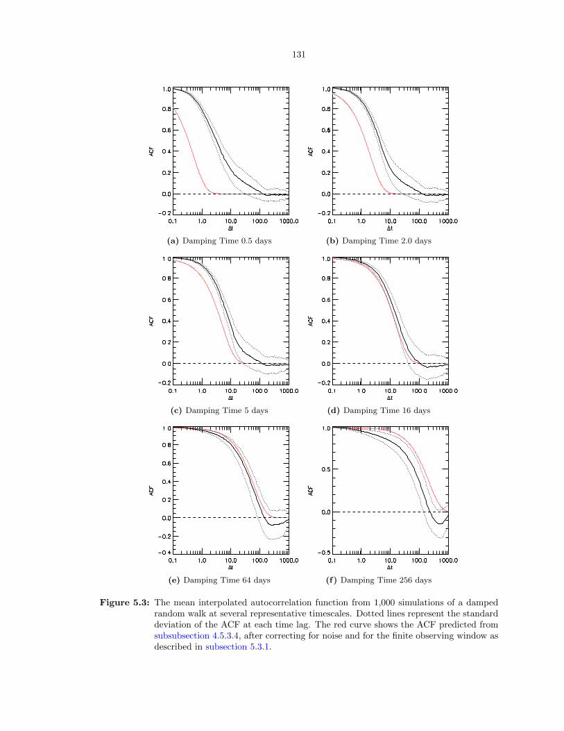
131

(a) Damping Time 0.5 days (b) Damping Time 2.0 days

(c) Damping Time 5 days (d) Damping Time 16 days

(e) Damping Time 64 days (f) Damping Time 256 days

Figure 5.3: The mean interpolated autocorrelation function from 1,000 simulations of a dampedrandom walk at several representative timescales. Dotted lines represent the standarddeviation of the ACF at each time lag. The red curve shows the ACF predicted fromsubsubsection 4.5.3.4, after correcting for noise and for the finite observing window asdescribed in subsection 5.3.1.

132

(a) Output Timescale for Sine (b) Output Timescale forSquared Exponential Gaus-sian Process

(c) Output for Damped RandomWalk

(d) Timescale Repeatability forSine

(e) ... for Squared ExponentialGaussian Process

(f) ... for Damped Random Walk

(g) Timescale Discrimination forSine

(h) ... for Squared ExponentialGaussian Process

(i) ... for Damped Random Walk

Figure 5.4: The timescale calculated from the autocorrelation function, plotted as a function ofthe true underlying timescale. Only simulations with no measurement noise are shown.Top panels show the ratio of the output timescale to the value predicted in section 4.5.Middle panels show the ratio of the standard deviation to the mean output timescale.Bottom panels show the degree by which the input timescale has to change to signifi-cantly affect the output timescale. In all plots, blue represents the time at which theautocorrelation function first falls below 1/9, orange the time at which it falls below1/4, and green the time at which it falls below 1/2.

133

5.3.3.2 Precision

In the middle two panels of Figure 5.4, the scatter in the estimated timescale across multiple simu-

lation runs is plotted for three different timescale metrics. For both sinusoidal and damped random

walk lightcurves, cutting the autocorrelation function at 1/2 generally yields less scatter than cutting

at 1/4 or 1/9.

5.3.3.3 Discrimination

Discrimination is a measure of how well the inferred timescale correlates with the true lightcurve

timescale. Good discrimination requires both a strong dependence of output on input timescale and

high repeatability for individual timescale measurements. Poor discrimination means a timescale

metric cannot be used to separate short- and long-timescale lightcurves with any fidelity.

In the bottom two panels of Figure 5.4, the scatter in the estimated timescale across multiple

simulation runs is plotted for three different timescale metrics. The discrimination is not defined

at short sine periods because the output timescale decreases with the true period (cf. Figure 5.2).

At longer sine periods, the inferred timescale correlates well with the period and the discriminatory

power is comparable to the scatter in the individual measurements. For the damped random walk,

the inferred timescale correlates poorly with the true timescale, so the discrimination is much poorer

than the scatter alone would imply. While the true timescale of a long-period sinusoidal signal can

be inferred to 10% or better, the accuracy of the same estimate for a damped random walk is only

70-80% at best.

5.3.3.4 Sensitivity to Noise

The average value of the autocorrelation timescale changes very little between an effectively infinite

signal-to-noise and a signal-to-noise ratio of 10. At a signal-to-noise ratio of 4, on the other hand,

the calculated timescale shows much less variation with the true timescale. This is particularly

dramatic for the sine wave (upper left panel), since for signal-to-noise of 10 or greater, the calculated

timescale is proportional to the period for periods of 16 days or longer, while for signal-to-noise of

4 the proportionality disappears.

The scatter in individual measurements is more sensitive to signal-to-noise. The degree to which

noise degrades measurement precision is independent of the true timescale. Again, signal-to-noise

of 4 is significantly different from signal-to-noise of 10 or higher.

The discriminating power of timescales based on autocorrelation functions shows a similar de-

pendence on signal-to-noise as the scatter. Discrimination gets poorer at low signal-to-noise in a

manner independent of the true timescale.

134


(c) Output Timescale forDamped Random Walk


(e) Timescale Repeatability forSquared Exponential Gaus-sian Process

(f) Timescale Repeatability forDamped Random Walk


(h) Timescale Discrimination forSquared Exponential Gaus-sian Process

(i) Timescale Discrimination forDamped Random Walk

Figure 5.5: As Figure 5.4, but plotting only the timescale at which the autocorrelation functionfirst falls below 1/2. Blue represents zero noise, orange represents a signal-to-noiseratio of 20, green a signal-to-noise ratio of 10, and black a signal-to-noise ratio of 4.All lightcurves have an expected 5-95% amplitude of 0.5 magnitudes.

135

5.3.3.5 Sensitivity to Cadence

The behavior of the interpolated autocorrelation function is similar for the two PTF cadences and

the YSOVAR cadence (Figure 5.6), except in their characteristic scales. Timescales calculated for

lightcurves sampled with the full PTF cadence are systematically higher than those calculated for the

PTF cadence in 2010, which are in turn higher than those for lightcurves sampled at the YSOVAR

cadence.

For sinusoidal lightcurves sampled at either PTF cadence, the autocorrelation timescale correlates

with the period for periods larger than or comparable to 16 days. For the YSOVAR sampling, the

timescale is reliable for periods of 5 days or longer. The autocorrelation timescale is never well

correlated with the period for a damped random walk, regardless of sampling. The fractional

scatter shows no strong trends with the input timescale for either sampling or for either type of

lightcurve. The discriminating power is best at long timescales for a sinusoidal signal, but is best at

intermediate timescales (relative to the cadence and time baseline of the observations) for a damped

random walk.

In general, the interpolated autocorrelation function performs best at the YSOVAR cadence,

worse at the 2010-only PTF cadence, and worst of all at the full PTF cadence, as measured by

output timescale bias or discriminating power. In Table 5.1, the YSOVAR cadence has the smallest

maximum gap in the data, the smallest time base line, and the fewest points of the three cadences;

the full PTF cadence has the largest maximum gap, the longest base line, and the most points. Of

these properties, the maximum gap is most likely the one that controls ACF performance: after

interpolation, the gap will be filled with a perfectly linear time series that an autocorrelation solver

cannot distinguish from real data.

Neither characteristic cadence nor, surprisingly, linearity of the time series correlates with ACF

performance; the YSOVAR cadence is intermediate between the two PTF cadences in both metrics.

5.3.4 Summary

In Chapter 4, I showed that the autocorrelation function can be converted into a timescale by finding

the time lag at which it crosses some threshold. The resulting timescales are consistent to within

a few tens of percent across different types of lightcurves, and they are, at least in the ideal case,

proportional to the true timescale, making them versatile and accurate as defined in section 5.1.

To estimate the autocorrelation function for real, irregularly sampled data, I considered in this

section interpolating the data to a high-cadence, regular grid. This interpolation introduces signif-

icant artifacts into the autocorrelation function. These artifacts dominate the inferred timescale,

giving results that correlate weakly with the true period except in the case of a long-period sinusoidal

signal. The performance depends little on signal-to-noise but is extremely sensitive to the cadence.

136









Figure 5.6: As Figure 5.4, but plotting only the timescale at which the autocorrelation functionfirst falls below 1/2. Orange represents the full PTF cadence, blue the PTF cadencein 2010 alone, and green the YSOVAR cadence.

137

I do not recommend the use of autocorrelation functions as a timescale metric, except possibly

in cases where the cadence has no gaps on timescales comparable to or larger than the variability.

For irregular cadences, this metric is neither accurate nor dependable.

5.4 Scargle Autocorrelation Functions

We attempted to implement an autocorrelation function for irregular sampling in terms of the

power spectrum, following Scargle (1989). While we were able to use the discrete Fourier transform

to estimate the power spectrum of the data for arbitrary sampling, we found that the resulting

autocorrelation function had severe systematics such as high-frequency oscillations. These appear

to be an artifact of computing the power spectrum over a limited frequency range, usually neglecting

high frequencies, and of aliases in the power spectrum.

We were unable to determine either an appropriate frequency cutoff or a way to apodize the

frequencies naturally, so we did not run the grid of lightcurve tests described elsewhere in this

chapter. While the Scargle (1989) ACF is a mathematically well-justified approach to calculating

ACFs, the problem of how to correctly filter the frequency spectrum must be addressed before its

robustness may be tested.

5.5 ∆m-∆t Plots

The general properties of ∆m-∆t plots were presented in section 4.6. For ∆m-∆t plots with a finite

number of samples, I estimated the quantiles of ∆m as a function of ∆t by binning the (∆t,∆m)

pairs in ∆t, and calculating the appropriate quantile within each bin. This is effectively taking a

histogram of the data in ∆m-∆t space, with all the disadvantages thereof, but it is the simplest

implementation. Timescales are then defined by finding the low end of the first ∆t bin in which a

particular quantile of ∆m exceeds a set threshold.

In the analysis presented here, the first bin edge was set at 10−1.97 days, with subsequent bins

at increments of 0.15 dex up to the full lightcurve baseline. This choice of bins allowed all possible

timescales to be probed, even in the highest-cadence portions of our data, while our nightly observing

gap would only deplete points from two bins, from 10−0.47 days to 10−0.32 days and from 10−0.32 days

to 10−0.17 days.

In practice, the variance in timescales across different realizations of the same lightcurve generator

usually exceeds the ∼ 40% quantization introduced by 0.15 dex bins. Therefore, finer bins would

not improve performance, and are likely to worsen it by increasing the scatter in each bin.

The use of ∆t bins in analyzing the ∆m-∆t plot quantizes the output timescale to one of the

bin edges. While the scatter in most simulation runs exceeds the bin width, in some runs enough of

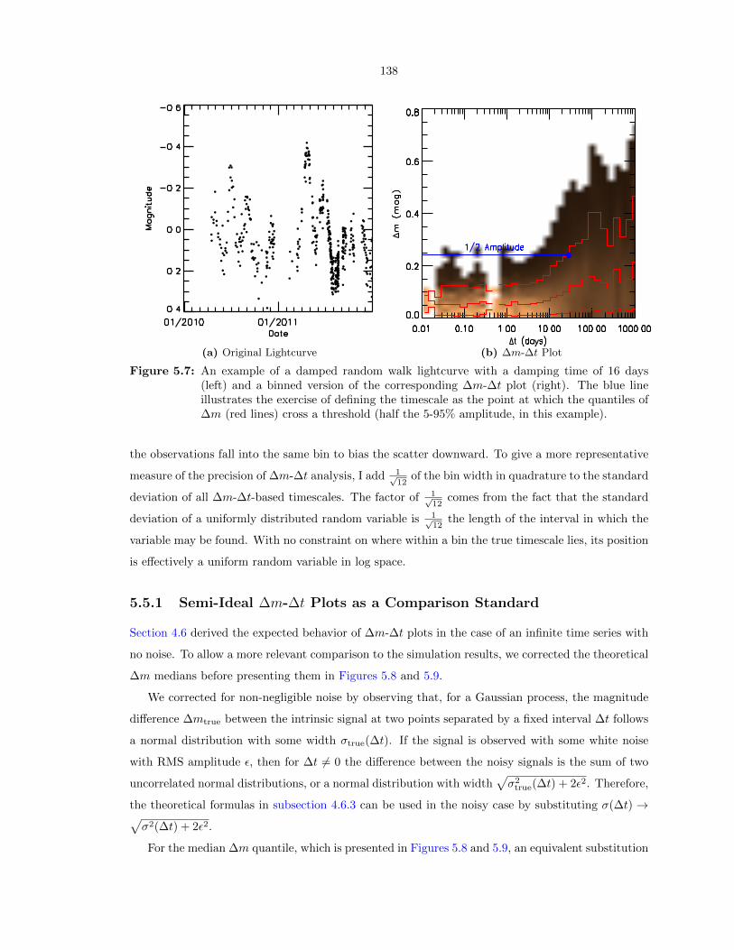
138

(a) Original Lightcurve (b) ∆m-∆t Plot

Figure 5.7: An example of a damped random walk lightcurve with a damping time of 16 days(left) and a binned version of the corresponding ∆m-∆t plot (right). The blue lineillustrates the exercise of defining the timescale as the point at which the quantiles of∆m (red lines) cross a threshold (half the 5-95% amplitude, in this example).

the observations fall into the same bin to bias the scatter downward. To give a more representative

measure of the precision of ∆m-∆t analysis, I add 1√12

of the bin width in quadrature to the standard

deviation of all ∆m-∆t-based timescales. The factor of 1√12

comes from the fact that the standard

deviation of a uniformly distributed random variable is 1√12

the length of the interval in which the

variable may be found. With no constraint on where within a bin the true timescale lies, its position

is effectively a uniform random variable in log space.

5.5.1 Semi-Ideal ∆m-∆t Plots as a Comparison Standard

Section 4.6 derived the expected behavior of ∆m-∆t plots in the case of an infinite time series with

no noise. To allow a more relevant comparison to the simulation results, we corrected the theoretical

∆m medians before presenting them in Figures 5.8 and 5.9.

We corrected for non-negligible noise by observing that, for a Gaussian process, the magnitude

difference ∆mtrue between the intrinsic signal at two points separated by a fixed interval ∆t follows

a normal distribution with some width σtrue(∆t). If the signal is observed with some white noise

with RMS amplitude ε, then for ∆t 6= 0 the difference between the noisy signals is the sum of two

uncorrelated normal distributions, or a normal distribution with width√σ2

true(∆t) + 2ε2. Therefore,

the theoretical formulas in subsection 4.6.3 can be used in the noisy case by substituting σ(∆t) →√σ2(∆t) + 2ε2.

For the median ∆m quantile, which is presented in Figures 5.8 and 5.9, an equivalent substitution

139

is ∆m →√

∆m2 + (0.67449√

2ε)2, where the expression in parentheses is the median ∆m for a

white noise process with variance 2ε2. While this expression is correct only for Gaussian process

lightcurves, we also used it to transform the theoretical expectations for a sine in Figures 5.8, since

it at least has the correct behavior in the limiting cases where the noise is much more than or much

less than the expected variation.


5.5.2.1 Sinusoid

I present in Figure 5.8 the average value of the ∆m median for a set of 1,000 simulations of a

sinusoidal lightcurve with different periods, along with the theoretical prediction derived in the

previous chapter. The values of ∆m in each bin generally follow the predictions, although in most

bins ∆m is averaged over multiple cycles.


I present in Figure 5.9 the average value of the ∆m median for a set of 1,000 simulations of a damped

random walk with different correlation times, along with the theoretical prediction derived in the

previous chapter. The average behavior of the ∆m median is close to the prediction, but there is a

large amount of scatter from run to run.


∆m-∆t plots for a squared exponential Gaussian process qualitatively resemble those for a damped

random walk, in that they resemble theoretical predictions on average but have a large degree of

scatter from run to run. The ∆m-∆t plots for a random walk also resemble predicted behavior on

average, but with nearly 100% scatter for bins probing timescales longer than 200 days. The rise

in scatter suggests that ∆m-∆t plots cannot accurately represent variability on large fractions (∼

1/5) of the observing baseline; the lightcurve provides an unrepresentative snapshot of variability

on longer timescales, and the ∆m-∆t plot cannot present information that is not in the data.

5.5.3 Performance


In Figure 5.10, I compare the performance of two different timescales, both derived by finding the

value of ∆t at which the 90th percentile of ∆m first rises above a particular threshold. In the

top two panels, the timescale calculated from simulations is divided by the corresponding timescale

140




Figure 5.8: The average value of the ∆m median from 1,000 simulations of a sine wave at sev-eral representative periods. Error bars represent the standard deviation of the ∆mmedian in each ∆t bin. The red curve shows the ∆m median predicted from Equa-tion 4.31, after correcting for noise and for the finite observing window as described insubsection 5.5.1.

141




Figure 5.9: The average value of the ∆m median from 1,000 simulations of a damped randomwalk at several representative timescales. Error bars represent the standard deviationof the ∆m median in each ∆t bin. The red curve shows the ∆m median predictedfrom Equation 4.47, after correcting for noise and for the finite observing window asdescribed in subsection 5.5.1.

142

from section 4.6; the dotted line across the middle of the plot represents behavior consistent with

analytical theory.

For sinusoidal signals, the calculated timescale is in general consistent with analytical results.

For damped random walks, the calculated timescale is consistent with theory for damping times up

to 16 days; walks with timescales of 64 days or longer see a fall-off of up to a factor of three as the

∆m-∆t plot no longer has a representative sampling of the variability.

5.5.3.2 Precision

The middle two panels of Figure 5.10 show the scatter in the estimated timescale multiple simulation

runs. For sinusoidal signals, the scatter is of order 10%. For 2-day periods the scatter is much higher

because at that period the largest change in the signal is over time intervals from half a day to a

day, which our nightly cadence samples very poorly. For the damped random walk, the scatter is of

order 40% for short timescale variables, and 50% or larger at long timescales. The timescale defined

as the point where ∆m crosses one half of the lightcurve amplitude has slightly less scatter than the

analogous timescale defined at one third of the amplitude.


The bottom two panels of Figure 5.10 show the smallest difference in input timescale that can be

distinguished using the output timescale. Since the ∆m-∆t timescale is, in general, proportional

to the true timescale, the discrimination is set by the scatter in the estimated timescale. For long

timescale damped random walks, the drop-off in output timescale is reflected in a reduced ability to

discriminate between timescales differing by less than a factor of two.


Figure 5.11 shows the performance of a ∆m-∆t timescale as a function of the signal-to-noise ratio of

the lightcurve. The average value of the timescale changes very little between an effectively infinite

signal-to-noise and a signal-to-noise ratio of 20, particularly for a sinusoidal signal. At a signal-to-

noise ratio of 4, on the other hand, the calculated timescale is always close to the smallest timescale

sampled, suggesting that the ∆m-∆t plot is dominated by noise.

The scatter in individual measurements rises smoothly with decreasing signal-to-noise. The

degree to which noise degrades measurement precision is independent of both the lightcurve shape

and the true timescale. The discriminating power of the timescale metric degrades similarly, although

for a damped random walk the power is more sensitive to signal-to-noise at short timescales than at

long timescales.

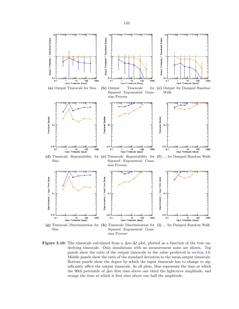
143









Figure 5.10: The timescale calculated from a ∆m-∆t plot, plotted as a function of the true un-derlying timescale. Only simulations with no measurement noise are shown. Toppanels show the ratio of the output timescale to the value predicted in section 4.6.Middle panels show the ratio of the standard deviation to the mean output timescale.Bottom panels show the degree by which the input timescale has to change to sig-nificantly affect the output timescale. In all plots, blue represents the time at whichthe 90th percentile of ∆m first rises above one third the lightcurve amplitude, andorange the time at which it first rises above one half the amplitude.

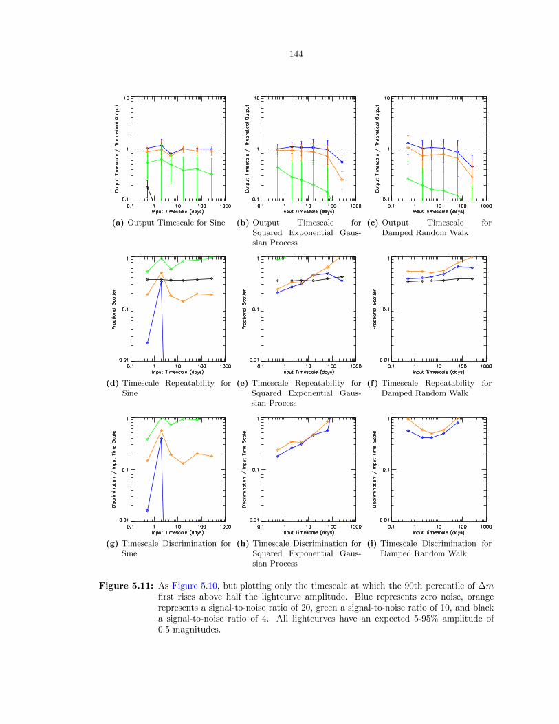
144









Figure 5.11: As Figure 5.10, but plotting only the timescale at which the 90th percentile of ∆mfirst rises above half the lightcurve amplitude. Blue represents zero noise, orangerepresents a signal-to-noise ratio of 20, green a signal-to-noise ratio of 10, and blacka signal-to-noise ratio of 4. All lightcurves have an expected 5-95% amplitude of0.5 magnitudes.

145


In Figure 5.12, I compare the behavior of a ∆m-∆t timescale for the two PTF cadences and the

YSOVAR cadence. For sinusoidal signals sampled at the full PTF cadence, the timescale is pro-

portional to the period for periods from half a day to 256 days. At the 2010 only cadence, the

timescale is well behaved for periods of 6 days or longer, but systematically too high for periods of

2 days or shorter. At the YSOVAR cadence, the timescale is proportional to the period for periods

of two days and longer, but not for one day or shorter. For all three cases, the “turnoff” in the plot

appears to happen at around the characteristic cadence (see Table 5.1.2 for a definition) or by at

most twice this value; the grid is too coarse to make a precise assessment. This suggests that the

∆m-∆t timescale cannot properly assess timescales that are not well sampled by the data.

The ∆m-∆t timescale shows a somewhat different behavior for damped random walks. At the

full PTF cadence, the timescale is proportional to the damping time for timescales between half

a day and 64 days. At the 2010 PTF cadence and at the YSOVAR cadence, there is no obvious

interval over which the ∆m-∆t timescale is proportional to the true timescale. At short timescales,

the timescale is overestimated, possibly for the same reasons as for short periods in the sinusoidal

case. At long timescales, the timescale is underestimated, because the observed lightcurve no longer

probes the slowest variability in the system (cf. the ∆m-∆t plots in Figure 5.9).

When applied to a sinusoidal signal, a ∆m-∆t timescale has slightly more scatter on the YSOVAR

cadence (∼ 30%) than on either of the PTF cadences (∼ 20%). When applied to a damped random

walk, the timescale has the most scatter on the YSOVAR cadence (∼ 100%) and the least on the full

PTF cadence (∼ 50%). The ability to discriminate input timescales follows a similar pattern. This

scaling is most likely driven by either the number of points or the time baseline of each lightcurve,

which is worst for the YSOVAR cadence and best for the full PTF cadence.

5.5.4 Summary

In Chapter 4, I showed that a ∆m-∆t plot can be converted to a scalar timescale by finding the ∆t bin

in which a predetermined quantile of ∆m first rises above some threshold. The resulting timescales

vary by roughly a factor of two across different types of lightcurves, but they are proportional to the

true timescale, at least in the ideal case. As a result, ∆m-∆t plots are accurate but not versatile, in

the sense defined in section 5.1.

I considered in this section the behavior of the ∆m-∆t plot and associated timescales when

applied to finite, noisy data sets. Even when given imperfect data, the ∆m-∆t timescale correlates

well with the true timescale of the lightcurve, confirming that it remains accurate even under realistic

conditions. However, the behavior of individual lightcurves introduces a lot of scatter into the ∆m-

∆t timescale, with a typical standard deviation as high as 50-70%. Therefore, ∆m-∆t timescales

146









Figure 5.12: As Figure 5.10, but plotting only the timescale at which the 90th percentile of ∆m firstrises above half the lightcurve amplitude. Orange represents the full PTF cadence,blue the 2010-only PTF cadence, and green the YSOVAR cadence.

147

are not precise.

The ∆m-∆t timescales are moderately sensitive to the presence of noise in the lightcurve. Noise

biases the inferred timescale downward; the effect is moderate if the noise RMS is at most one

tenth the lightcurve amplitude, but quickly grows more severe at higher noise levels. The ∆m-∆t

timescale also requires a cadence with a high dynamic range of sampling; it will overestimate the

timescale for sources varying faster than about ∼ 1 − 2 times the characteristic cadence, and will

underestimate the timescale if the true timescale is greater than about 1/15 of the monitoring base

line (Figure 5.12c). While the ∆m-∆t timescale keeps rising with input timescale past this point,

“saturating” only at about 1/5 the base line (the case represented by the undamped random walk

model), the discriminating power of the ∆m-∆t timescale is worse than a factor of two at these long

timescales. Therefore, the ∆m-∆t timescale is only dependable in a limited sense.

The ∆m-∆t timescale is a potentially useful timescale metric if the data are observed with a

high dynamic range cadence, with a coverage window at least ∼ 30 times the sampling interval, and

if the 5-95% amplitude of the variability is at least ten times the RMS of the noise. However, even

then the timescales should be assumed to have a 1σ uncertainty of ∼ 50%. The ∆m-∆t timescale

may be more appropriate for ensemble studies than for characterizing individual lightcurves.

5.6 Peak-Finding

Peak-finding is a timescale metric developed by Cody et al. (2014) for well-sampled aperiodic

lightcurves. We use a slightly older version of the method from that presented by Cody et al.,

which begins with the first point on the lightcurve, then identifies the first local minimum or max-

imum that differs from the first point by a predetermined magnitude threshold. After each local

minimum it finds the first local maximum differing from it by the threshold, and vice versa. In

this way, the method builds up a list of alternating minima and maxima, discarding low-amplitude

fluctuations. The mean time between minima and maxima separated by a given amplitude threshold

is a measure of the speed of fluctuations of that amplitude. By repeating the process for a variety

of thresholds, one builds up a plot (Figure 5.13) of timescale as a function of magnitude scale, from

the level of measurement noise up to the full lightcurve amplitude.

For this study we have altered the algorithm of Cody et al. (2014) by considering the median

separation between fluctuations, rather than the mean. The mean separation would be biased high

by the large seasonal gaps in our data set. The median separation is much more robust to coverage

gaps provided that most of the variability is on timescales shorter than the length of a season,

because then the many minima and maxima within each season’s coverage dominate the median.

In the analysis presented here, the median peak separation was calculated at each multiple of

0.01 mag, up to the full lightcurve amplitude. The resulting peak-finding plot was converted into a

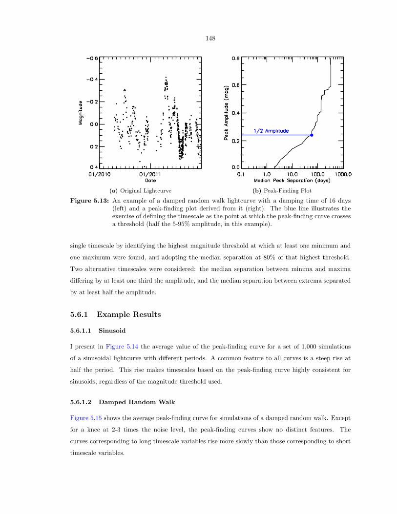
148

(a) Original Lightcurve (b) Peak-Finding Plot

Figure 5.13: An example of a damped random walk lightcurve with a damping time of 16 days(left) and a peak-finding plot derived from it (right). The blue line illustrates theexercise of defining the timescale as the point at which the peak-finding curve crossesa threshold (half the 5-95% amplitude, in this example).

single timescale by identifying the highest magnitude threshold at which at least one minimum and

one maximum were found, and adopting the median separation at 80% of that highest threshold.

Two alternative timescales were considered: the median separation between minima and maxima

differing by at least one third the amplitude, and the median separation between extrema separated

by at least half the amplitude.


5.6.1.1 Sinusoid

I present in Figure 5.14 the average value of the peak-finding curve for a set of 1,000 simulations

of a sinusoidal lightcurve with different periods. A common feature to all curves is a steep rise at

half the period. This rise makes timescales based on the peak-finding curve highly consistent for

sinusoids, regardless of the magnitude threshold used.


Figure 5.15 shows the average peak-finding curve for simulations of a damped random walk. Except

for a knee at 2-3 times the noise level, the peak-finding curves show no distinct features. The

curves corresponding to long timescale variables rise more slowly than those corresponding to short

timescale variables.

149




Figure 5.14: The mean peak-finding function from 1,000 simulations of a sine wave at severalrepresentative periods. Dotted lines represent the standard deviation of the peak-finding function at each time lag.

150




Figure 5.15: The mean peak-finding function from 1,000 simulations of a damped random walkat several representative timescales. Dotted lines represent the standard deviation ofthe peak-finding function at each time lag.

151


On a squared exponential Gaussian process, a peak-finding plot shows a leveling out on long

timescales, indicating that high-amplitude minima and maxima rapidly become rare for these lightcurves.

However, the peak-finding plot varies too much from lightcurve to lightcurve for this feature to serve

as a useful timescale metric. On a random walk, which has no characteristic timescale, the peak-

finding plot generally slopes upward, as it does for a damped random walk. However, the peak-finding

plot for a random walk has many irregularities, including areas where it levels out.

5.6.2 Performance


In Figure 5.16, I compare the performance of three different timescales, each defined as the time

separation at which the peak-finding curve crosses a different threshold: one third the lightcurve

amplitude, one half the lightcurve amplitude, or 80% of the highest ∆m in the peak-finding curve.

The highest ∆m can be anywhere between half the lightcurve amplitude and its full amplitude,

depending on the phase at which the lightcurve is initially observed.

For sinusoidal signals, the calculated timescale is proportional to the period for periods of two

days or longer, and varies little with the choice of cutoff value. One exception is the time at which the

peak-finding curve crosses one third the amplitude, which is biased low by a “bump” at timescales of

two days (visible in Figure 5.14f) that may be the result of high-σ outliers in the noise. For damped

random walks, the calculated timescale increases with the damping time, but at a slower rate than a

strict proportionality. The time at which the peak-finding curve crosses 80% of its maximum comes

closest to a linear dependence on the true timescale. In neither case do the inferred timescales ever

fall below one day; the median separation between peaks is always at least one day even if the

magnitude threshold is lowered far enough to probe noise.

5.6.2.2 Precision

The middle two panels of Figure 5.16 show the scatter in the estimated timescale over multiple

simulation runs. For sinusoidal signals, the scatter is negligible for all but the shortest and longest

periods. The scatter in the timescale is much larger for damped random walks; it is on the order

of 20% for short timescale lightcurves, but grows to over 100% at longer timescales. The times at

which the peak-finding curve crosses one third and one half the amplitude have consistently less

scatter than timescales based on 80% of the tip of the peak-finding plot.

152









Figure 5.16: The timescale calculated from a peak-finding plot, plotted as a function of the trueunderlying timescale. Only simulations with no measurement noise are shown. Toppanels show the average value of the output timescale. Middle panels show the ratioof the standard deviation to the mean output timescale. Bottom panels show thedegree by which the input timescale has to change to significantly affect the outputtimescale. In all plots, blue represents the time at which the peak-finding curve firstrises above one third the lightcurve amplitude, orange the time at which it rises aboveone half the amplitude, and green the time at which the peak-finding curve crosses80% of its highest value.

153


Because the peak-finding timescale is linear with the period for a sine, the discrimination shows

the same behavior as the scatter. Because the peak-finding timescale grows more slowly than

the damping time for a damped random walk, and even levels out for long timescale signals, the

discriminating power of the peak-finding plot is never better than 40%. The discriminatory power

does not depend on how the peak-finding plot is converted to a timescale: timescales based on 80%

of the highest point in the plot show more scatter but also scale better with the lightcurve timescale

on average, and the advantage and disadvantage compared to timescales measured at a fixed fraction

of the amplitude cancel out.


Figure 5.17 shows the performance of a peak-finding timescale as a function of the signal-to-noise

ratio of the lightcurve. The average value of the timescale changes very little between an effectively

infinite signal-to-noise and a signal-to-noise ratio of 20 in the case of a sinusoidal signal, but decreases

systematically with signal-to-noise in the case of a damped random walk. In both cases, at signal-

to-noise of 10 or less the peak-finding timescale is barely correlated with the true timescale.

The precision of timescale measurements of a sinusoidal signal generally increases with signal-

to-noise, as one might expect. The precision of timescale measurements of a damped random walk,

on the other hand, decreases with signal-to-noise. This may indicate that at low signal-to-noise the

timescale is strongly affected by a fixed systematic term.

The discriminating power of the peak-finding timescale roughly follows the precision for a sine

wave, but is substantially poorer — no better than 30% — than the precision for a damped random

walk. As noted above, for signal-to-noise of 10 or less the peak-finding timescale cannot discriminate

between short- and long-timescale signals.


In Figure 5.18, I compare the behavior of a peak-finding timescale for both PTF cadences and the

YSOVAR cadence. For sinusoidal signals sampled at either the full PTF cadence or the YSOVAR

cadence, the timescale is proportional to the period for periods of two days or more. For the more

sparsely sampled 2010-only PTF cadence, peak-finding overestimates the period for a 2-day sine

by nearly a factor of two. The average behavior of the peak-finding timescale, when applied to a

damped random walk, is qualitatively similar regardless of the lightcurve cadence.

The peak-finding timescale shows the least scatter for lightcurves observed with the full PTF

cadence, more for lightcurves observed with the 2010-only PTF cadence, and the highest amount

of scatter for the YSOVAR cadence. This is true regardless of whether the timescale is measured

154









Figure 5.17: As Figure 5.16, but plotting only the timescale at which the peak-finding curve firstreaches one half the lightcurve amplitude. Blue represents zero noise, orange rep-resents a signal-to-noise ratio of 20, green a signal-to-noise ratio of 10, and blacka signal-to-noise ratio of 4. All lightcurves have an expected 5-95% amplitude of0.5 magnitudes.

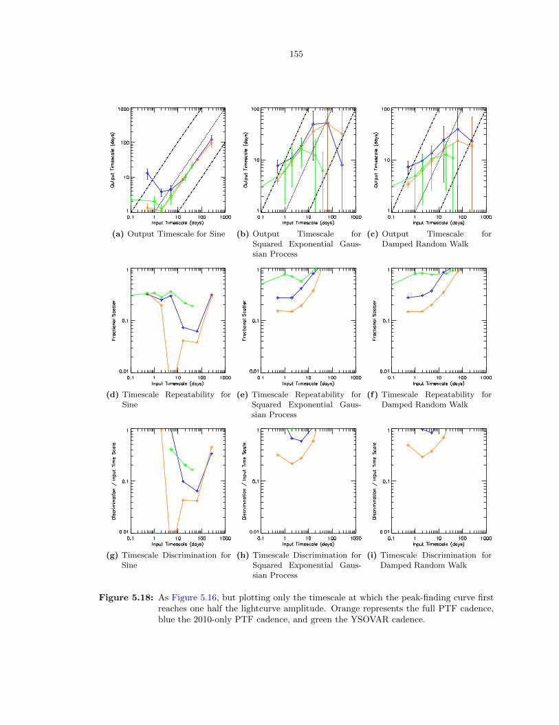
155









Figure 5.18: As Figure 5.16, but plotting only the timescale at which the peak-finding curve firstreaches one half the lightcurve amplitude. Orange represents the full PTF cadence,blue the 2010-only PTF cadence, and green the YSOVAR cadence.

156

for sinusoidal signals or for damped random walks. The discriminating power shows a similar trend

with signal-to-noise ratio.

5.6.3 Summary

Because it is based on extrema of a lightcurve rather than its average behavior, peak-finding does

not lend itself easily to analytical treatment and was not studied in Chapter 4. The numerical

simulations presented in this section suggest that, while the peak-finding timescale correlates with

the input timescale for a variety of lightcurves, the shape of the scaling is sensitive to the type of

lightcurve. In the sense of section 5.1, it is accurate but not versatile.

For rapidly varying signals the peak-finding timescale shows a scatter of ∼10-20% for long time

series such as the PTF cadences, but somewhat more scatter (∼ 40%) for lightcurves observed

with the YSOVAR cadence. Regardless of cadence, the scatter grows to a factor of two for aperiodic

lightcurves with timescales longer than 1/15 to 1/20 the observing base line. Therefore, peak-finding

timescales are not precise except for time series many times longer than the signals of interest.

The peak-finding timescales are moderately sensitive to the presence of noise in the lightcurve.

Noise biases the inferred timescale downward; the effect is moderate if the noise RMS is at most one

tenth the lightcurve amplitude, but quickly grows more severe at higher noise levels. The average

behavior of the lightcurve seems to depend little on the cadence adopted, showing a similar slope

(Figure 5.18c) up to timescales of order the time series base line. As noted above, the timescale

needs a long time series to provide precise measurements. The timescale therefore is not dependable:

its performance depends on both signal-to-noise and the cadence.

The peak-finding timescale is best suited for long-term monitoring of short-timescale variability.

The 5-95% amplitude of the variability should be at least ten times the RMS of the noise to ensure

that noise does not confuse the peak-finding algorithm. Even then, the peak-finding timescale should

be interpreted only in an ordinal sense; it can determine which lightcurves vary more rapidly than

others, but may get the absolute timescale wrong by as much as an order of magnitude.

5.7 Gaussian Process Modeling

Gaussian process regression is an increasingly popular analysis tool for modeling aperiodic time

series that are assumed to consist of a smooth (but unknown) function plus noise. Since a Gaussian

process has no specific functional form, a good fit is instead characterized by a high likelihood that

the data were drawn from a Gaussian distribution with a particular covariance matrix.

In the most common case, the one I use here, the covariance matrix K is assumed to be the sum

of a squared exponential Gaussian process, characterized by an amplitude σ and a coherence time

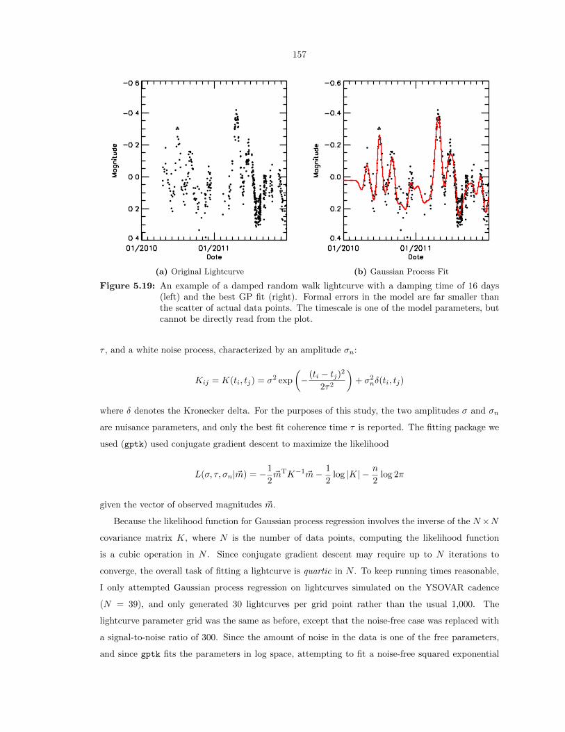
157

(a) Original Lightcurve (b) Gaussian Process Fit

Figure 5.19: An example of a damped random walk lightcurve with a damping time of 16 days(left) and the best GP fit (right). Formal errors in the model are far smaller thanthe scatter of actual data points. The timescale is one of the model parameters, butcannot be directly read from the plot.

τ , and a white noise process, characterized by an amplitude σn:

Kij = K(ti, tj) = σ2 exp

(− (ti − tj)2

2τ2

)+ σ2

nδ(ti, tj)

where δ denotes the Kronecker delta. For the purposes of this study, the two amplitudes σ and σn

are nuisance parameters, and only the best fit coherence time τ is reported. The fitting package we

used (gptk) used conjugate gradient descent to maximize the likelihood

L(σ, τ, σn|~m) = −1

2~mTK−1 ~m− 1

2log |K| − n

2log 2π

given the vector of observed magnitudes ~m.

Because the likelihood function for Gaussian process regression involves the inverse of the N ×N

covariance matrix K, where N is the number of data points, computing the likelihood function

is a cubic operation in N . Since conjugate gradient descent may require up to N iterations to

converge, the overall task of fitting a lightcurve is quartic in N . To keep running times reasonable,

I only attempted Gaussian process regression on lightcurves simulated on the YSOVAR cadence

(N = 39), and only generated 30 lightcurves per grid point rather than the usual 1,000. The

lightcurve parameter grid was the same as before, except that the noise-free case was replaced with

a signal-to-noise ratio of 300. Since the amount of noise in the data is one of the free parameters,

and since gptk fits the parameters in log space, attempting to fit a noise-free squared exponential

158

Gaussian process (lnσn = −∞) with a noisy squared exponential Gaussian process would never

converge.

5.7.1 Performance


Figure 5.21 shows the performance of timescales derived from Gaussian process fitting as a function

of the signal-to-noise ratio of the magnitude measurements. In many cases the fit failed to converge

at all, with the fraction of times in which the fit succeeded shown in Figure 5.20. The curves in

Figure 5.21 are only for those modeling attempts that returned a valid solution.

For sinusoidal signals, the calculated timescale is proportional to the period for periods of two

days or longer, while timescales for shorter sine periods tend to be higher than those for longer

periods. For squared exponential random walks, the timescale generally increases with the true

timescale except in low signal-to-noise simulations. For damped random walks, on the other hand,

the calculated timescale is always 1-4 days, with only a weak dependence on underlying timescale.

This might be because the damped random walk has substantial structure on timescales shorter

than the characteristic timescale, and Gaussian process fitting is reported to be dominated by the

most rapidly varying component (Miller, priv. comm. (2012)).

For all three types of lightcurves, the best fit timescale has a systematic trend in the sense that

the timescale is lower for lower signal-to-noise lightcurves. The same behavior was observed for ∆m-

∆t plots and for peak-finding, and just as in those cases the likely cause is that the noise (which,

by construction, has an infinitesimal timescale) is being mistaken for real variability. Why this

confusion should happen when fitting a model that explicitly includes a white noise term, however,

is unclear. It may be a bias introduced by the use of maximum-likelihood methods, combined with

a partial degeneracy in the model between a short timescale for the main process and a strong white

noise component. Choi et al. (2014) also encountered a bias towards short timescales when fitting

damped random walk models to noisy lightcurves; we may be seeing a related issue here.

Unlike the other timescale metrics described in this chapter, Gaussian process fitting provides an

uncertainty for the best fit timescale. The accuracy of these uncertainties is tested in Figure 5.20,

which plots

χ2 =∑i

(τi − 〈τi〉)2

σ2τi

where i denotes one of the 30 lightcurves in each run, τi is the timescale returned by the fit, and

στi is the error returned by the fit. In general, the formal errors reflect the true uncertainty in τ for

short timescale lightcurves, but grossly underestimate it for longer timescale lightcurves, with the

discrepancy growing at decreasing signal-to-noise. Curiously, even when the lightcurve is a squared

exponential process with noise — in other words, the model being fitted is perfectly accurate — the

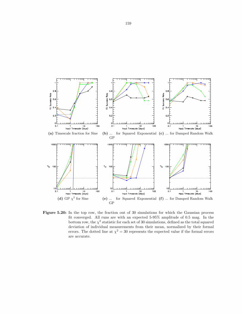
159

(a) Timescale fraction for Sine (b) ... for Squared ExponentialGP

(c) ... for Damped Random Walk

(d) GP χ2 for Sine (e) ... for Squared ExponentialGP


Figure 5.20: In the top row, the fraction out of 30 simulations for which the Gaussian processfit converged. All runs are with an expected 5-95% amplitude of 0.5 mag. In thebottom row, the χ2 statistic for each set of 30 simulations, defined as the total squareddeviation of individual measurements from their mean, normalized by their formalerrors. The dotted line at χ2 = 30 represents the expected value if the formal errorsare accurate.

160

scatter in τ still exceeds that predicted by the formal uncertainties. The excess scatter at long input

timescales may indicate that the time series no longer covers a long enough interval to sample the

full variability; given the steep dependence of running time on lightcurve length, we did not test any

extensions of the YSOVAR cadence.

5.7.1.2 Precision

The middle two panels of Figure 5.21 show the scatter in the estimated timescale over multiple

simulation runs. For sinusoidal signals and squared exponential Gaussian process signals, the scatter

is typically a few tens of percent. The scatter in the timescale is much larger for damped random

walks, on the order of 80% or more.


Because the Gaussian process fitting timescale is linear with the period for a sine, the discrimination

shows the same behavior as the scatter. Because the timescale grows very slowly with the damping

time for a damped random walk, the discriminating power of Gaussian process regression is never

better than a factor of two. The simulations with squared exponential Gaussian process lightcurves

are intermediate between these two cases, with good discriminating power at high signal-to-noise

but rapid degradation as the data get noisier.

5.7.1.4 Completeness

The Gaussian process fit rarely converges when applied to sines with periods shorter than 2 days,

has a roughly 40% convergence rate at 2 days, and has a high (> 90%) convergence rate at longer

periods. This threshold roughly corresponds to the period at which the timescale begins to show a

linear dependence on the period. There is no clear trend with signal-to-noise.

When applied to a short timescale squared exponential Gaussian process lightcurve, the fit con-

verges roughly 50% of the time, with higher rates for longer true timescales. Curiously, while for

timescales of 10 or 20 days the convergence rate is maximized at high signal-to-noise, for timescales

of 1 or 2 days the convergence rate is higher for a signal-to-noise ratio of 10 or 20 than at signal-to-

noise of 300. As with the sines, the change between these two regimes corresponds to a change in

the behavior of the timescale itself: at long periods, the timescale is systematically underestimated

at low signal-to-noise, just when the fraction of successful fits falls.

The rate of successful convergence is qualitatively the same for a damped random walk as for a

squared Gaussian process, except with a weaker dependence on signal-to-noise. There is no obvious

change in the behavior of the timescales at 5 days, when the convergence rate for low signal-to-noise

lightcurves begins to fall.

161


Figure 5.21 shows the performance of Gaussian process fitting as a function of the signal-to-noise

ratio of the lightcurve. When applied to either sinusoidal or squared exponential Gaussian processes,

the timescale inferred from Gaussian process fitting decreases systematically with signal-to-noise.

When applied to a damped random walk, the timescale shows no obvious trend with signal-to-noise,

but also seems to depend little on the intrinsic properties of the lightcurve.

The precision of timescale measurements of a sinusoidal signal or a squared exponential Gaussian

process signal generally increases with signal-to-noise, as one might expect. The fractional uncer-

tainty is 10-30% for mid-range timescales (1-10 days), but rises to 100% at timescales of 1 day or

shorter, and 20 days or longer for the Gaussian process. The scatter in timescale measurements also

increases at low signal-to-noise for a damped random walk, but to a much lesser degree than in the

other two cases.

The discriminating power of the Gaussian process timescale roughly follows the precision for a sine

wave and for a squared exponential Gaussian process, although in the latter case the degradation

with signal-to-noise is much steeper than for the precision. The Gaussian process has almost no

discriminating power when applied to a damped random walk, thanks to the combination of weak

average dependence on the damping timescale and high scatter from lightcurve to lightcurve.

5.7.2 Summary

While in principle Gaussian process models can be treated analytically, doing so in the limit of

infinite sampling as required by Chapter 4 would have been prohibitively complex. The numerical

simulations presented in this section suggest that the Gaussian process timescale is correlated with

the true timescale for some kinds of lightcurves but not others, so the metric is not accurate in the

sense of section 5.1. In addition, the fit does not always converge, for reasons unknown; it is, strictly

speaking, not universal.

I do not recommend the use of Gaussian process models as a timescale metric, unless the data are

known in advance to have only a small number of frequency components. For complex lightcurves,

such as damped random walks, the model results are inaccurate as well as computationally expensive.

5.8 Revisiting Bursters and Faders

Earlier in this chapter, I tested how well several candidate timescale metrics could reproduce the

known timescales of synthetic lightcurves. While informative, this test has the limitation that it

cannot be applied to real data, where the “true timescale” is necessarily unknown. A test that does

work for real data is desirable, if only for reassurance that the results of Chapter 4 and this chapter

162

(a) Output Timescale for Sine (b) ... for Squared ExponentialGP

(c) ... for Damped Random Walk


(e) ... for Squared ExponentialGP



(h) ... for Squared ExponentialGP


Figure 5.21: The timescale calculated from a squared exponential Gaussian process model, plottedas a function of the true underlying timescale. Only runs with an expected 5-95%amplitude of 0.5 mag are shown. Top panels show the average value of the outputtimescale. Middle panels show the ratio of the standard deviation to the mean outputtimescale. Bottom panels show the degree by which the input timescale has to changeto significantly affect the output timescale. In all plots, blue represents a signal-to-noise ratio of 300, orange represents a signal-to-noise ratio of 20, green a signal-to-noise ratio of 10, and black a signal-to-noise ratio of 4.

163

do not apply only to mathematically tractable signals.

Another criterion a good timescale metric should satisfy is that its output looks plausible under

visual inspection of the corresponding lightcurve. This is necessarily a subjective criterion, as con-

firmation bias (Nickerson, 1998, and references therein) ensures that there will be multiple, possibly

very different, values for a timescale that all look “reasonable” when a lightcurve is compared to

them a posteriori. Therefore, plausibility is a necessary but insufficient criterion, and should be

treated only as a supplement to the more objective tests presented in Chapter 4 and earlier in this

chapter.

For this test, I selected the 41 sources listed in Table 3.3 as having bursting or fading behavior.

I tested three timescale metrics on this set of lightcurves. The first was a ∆m-∆t plot with ∆t bins

in steps of 0.15 dex from 10−1.97 days to the maximum length of the lightcurve. The characteristic

timescale was defined to be the time bin in which the 90th percentile of the ∆m values first exceeds

half the lightcurve’s amplitude, itself defined as the difference between 5th and 95th percentiles. The

second metric was a peak-finding plot, with the characteristic timescale defined to be the separation

between peaks differing by at least half the lightcurve amplitude. The third metric was a Gaussian

process fit. The results are presented in Table 5.3.

Correlations between the computed and by-eye timescales are shown in Figures 5.22 and 5.23.

The ∆m-∆t timescale shows a weak correlation with both burst and fade width, but not with burst

or fade separation. The peak-finding timescale may be very weakly correlated with event width, but

it is not correlated with event separation. The Gaussian process timescale is not correlated at all

with any of the by-eye timescales.

I also inspected several lightcurves — those for LkHα 139, LkHα 174, FHO 15, FHO 19, FHO 25,

and FHO 26 — by eye to confirm whether the computed timescale metrics corresponded to real

structure in the lightcurve. For the lightcurve of FHO 26, I refer the reader to subsection 3.6.1. For

∆m-∆t timescales, the comparison was made by estimating the lightcurve amplitude by eye, then

searching for pairs of observations (not necessarily associated with bursting or fading) separated by

half that amplitude. The range of time separations between such pairs tended to include the ∆m-∆t

timescale, indicating that the timescale is at least roughly consistent with visual inspection of the

lightcurve. For peak-finding timescales, I estimated the lightcurve amplitude by eye, then searched

for local minima and maxima (again, not necessarily distinct bursting or fading events) separated by

at least half that amplitude. Depending on the lightcurve, the separations between these manually

identified peaks tended to be 2-3 times longer or 2-3 times shorter than the peak-finding timescale,

leaving the peak-finding results difficult to interpret.

∆m-∆t timescales seem easiest to relate to specific variations within the corresponding lightcurve.

Peak-finding timescales are harder to associate with specific structures, and the best-fit timescales

produced by Gaussian process models appear to have no correlation at all with any intuitive measure

164

Source Burst Burst Fade Fade ∆m-∆t Peak-Finding GaussianWidth(s) Separation(s) Width(s) Separation(s) Process

205032.32+442617.4 0.1-0.5 5-40 0.03 2 1.9 ± 0.5205036.93+442140.8 >352 >640 80 1,100 8.7 ± 0.4205040.29+443049.0 3.0 >165 1.8 11 0.48 ± 0.04205042.78+442155.8 0.04-0.12 1-313 0.02 3 26 ± 4205100.90+443149.8 2-3 13-39 1.3 10 1.06 ± 0.04205114.80+424819.8 47-56 96-334 10 100 10.2 ± 0.6205115.14+441817.4 120 >930 10 18205119.43+441930.5 1-2 4-7 0.3 5205120.99+442619.6 0.5-2.0 14-80 0.9 6205123.59+441542.5 43 560 1.8 4 1.04 ± 0.05205124.70+441818.5 1-3 7-10 0.6 5 0.38 ± 0.03205139.26+442428.0 6-7 22-50 2.5 18205139.93+443314.1 50-150 129-264 30 50205145.99+442835.1 100 >630 3 9 0.85 ± 0.05205155.70+443352.6 4-6 9-25 1.3 12205158.63+441456.7 0.5-3.0 7.0 4-16 83-327 1.3 8 0.52 ± 0.04205203.65+442838.1 36-119 685 0.01 9 2.1 ± 0.2205228.33+442114.7 1.5 5.78205230.89+442011.3 3 7.71 0.6 5 0.52 ± 0.02205252.48+441424.9 2-6 11-21 1.8 9 0.96 ± 0.04205253.43+441936.3 2-4 11-28 4 8 1.16 ± 0.09205254.30+435216.3 30-100 298-348 7 13 0.82 ± 0.05205314.00+441257.8 2-80 29-337 0.9 6 0.59 ± 0.04205315.62+434422.8 0.5-150 25-610 40 17 1.05 ± 0.03205340.13+441045.6 2-20 11-31 3-10 11-80 1.8 10 0.90 ± 0.04205410.15+443103.0 3 8-10 0.9 6 0.64 ± 0.04205413.74+442432.4 2-5 2-19 1.3 7205424.41+444817.3 5-11 250-330 0.6 6205445.66+444341.8 3-20 45-300 0.9 6 0.75 ± 0.06205446.61+441205.7 2-6 13-62 1.8 6 0.96 ± 0.05205451.27+430622.6 5-30 30-250 7 50 4.0 ± 0.3205503.01+441051.9 6 >57 4 12 1.17 ± 0.04205534.30+432637.1 65 >680 7 4 13.3 ± 1.8205659.32+434752.9 3-4 11-12 3 11 1.06 ± 0.05205759.84+435326.5 2.2-18 >100 0.9 5 0.51 ± 0.04205801.36+434520.5 14-37 29-90 80 71 1.24 ± 0.03205806.10+435301.4 1.5-5.0 35 1.3 6 0.94 ± 0.06205825.55+435328.6 2-6 8-123 0.9 6 0.72 ± 0.04205839.73+440132.8 0.5-4.0 8-210 14 19205905.98+442655.9 10-15 27-47 1.3 14205906.69+441823.7 2-3 8-63 0.9 4 0.43 ± 0.05

Table 5.3: The results of applying several timescale metrics to the sample of Table 3.3. Alltimescales are in days. The first four columns after the source name are the timescalesestimated by eye as described in Figure 3.4.1. The last three columns are the timescalesreturned by ∆m-∆t plots, peak-finding, and Gaussian process fitting, as described inthe text.

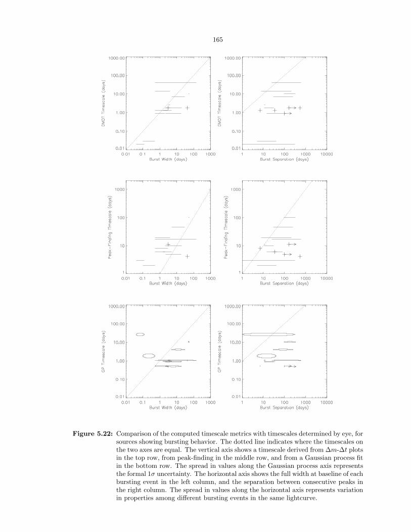
165

Figure 5.22: Comparison of the computed timescale metrics with timescales determined by eye, forsources showing bursting behavior. The dotted line indicates where the timescales onthe two axes are equal. The vertical axis shows a timescale derived from ∆m-∆t plotsin the top row, from peak-finding in the middle row, and from a Gaussian process fitin the bottom row. The spread in values along the Gaussian process axis representsthe formal 1σ uncertainty. The horizontal axis shows the full width at baseline of eachbursting event in the left column, and the separation between consecutive peaks inthe right column. The spread in values along the horizontal axis represents variationin properties among different bursting events in the same lightcurve.

166

Figure 5.23: As Figure 5.22, but for sources showing fading behavior.

167

of timescale. Although these results must be interpreted with caution, since I had preconceptions

about the effectiveness of the timescale metrics at the time I tested them on specific lightcurves,

the results are broadly consistent with the conclusion of section 5.9 that ∆m-∆t plots are the most

appropriate tool for this thesis.

5.9 Summary of Numerical Results

I present in Table 5.4 the simulated performance of each timescale metric according to the criteria

provided in section 5.1. This table is, to my knowledge, the first of its kind. While no single

metric satisfies all the criteria, ∆m-∆t Plots and Peak-Finding both perform well enough to warrant

careful use in real applications. Both metrics suffer from high variance, and both are sensitive to the

cadence: ∆m-∆t plots are only sensitive to timescales between the survey’s characteristic cadence

and 1/15 of the survey time base line, while peak-finding shows high scatter above 1/20-1/15 the

base line. In addition, no four of the metrics work well with signals with multiple timescales (see

Chapter 4), and none offer a significance test for the existence of a characteristic timescale.

I recommend the use of peak-finding for signals whose statistical properties are known a priori

(e.g., they are all well described by a particular model) as well as timescales much shorter than the

monitoring base line, and the use of ∆m-∆t plots for signals of unknown form but with timescales

known to be intermediate between the cadence and the maximum base line.

Criterion Interpolated ACF ∆m-∆t Plots Peak-Finding GP Modeling

Universal Yes Yes Yes NoData-Driven Tuning Param. Tuning Param. Yes YesVersatile to ∼ 20% to factor of 2 to factor of 2.5 to factor of 2.5Accurate 25-300% 20-100% 25-100% 6-600%Precise 10-60% 20-80% 10-100% 10-100%Dependable vs. Noise Yes Up to 1/10 amp. Up to 1/10 amp. NoDependable vs. Cadence No No NoRobust vs. OutliersRobust vs. Appended DataSignificance Test No No No No

Table 5.4: Performance of timescale metrics according to the criteria from section 5.1. See theindividual sections of this chapter for more details. A blank means the criterion wasnot tested.

Because they probe different parts of the lightcurve, timescales based on competing metrics

cannot be directly converted to each other; the conversion factor depends on the statistical properties

of a signal, which for a real lightcurve are usually unknown a priori. The distinction is similar to

the varying conversion factor between RMS amplitude and peak-to-peak amplitude for lightcurves

with different properties.

In Table 5.5, I show the ratio of all simulated timescales to ∆m-∆t timescales, which we use

extensively in Chapter 6, for each lightcurve model considered here. Simulated ACF timescales or

168

Timescale Metric Sinusoid Squared Exponential GP Damped Random Walk

Period ∼ 7τ∆m-∆t N / A N / ASimulated ∆m-∆t 90% quantile crosses 1/2 amp τ∆m-∆t τ∆m-∆t τ∆m-∆t

Simulated peak-finding crosses 1/2 amp ∼ 3τ∆m-∆t ∼ 2τ∆m-∆t ∼ 2τ∆m-∆t

Simulated peak-finding crosses 80% of peak-finding max ∼ 3τ∆m-∆t ∼ 6τ∆m-∆t ∼ 6τ∆m-∆t

Table 5.5: Output of each timescale metric, normalized by the ∆m-∆t timescale for ease of com-parison in Chapter 6. This table can be used to convert between different timescalemetrics by dividing each column by the timescale to be converted from. For exam-ple, the period is usually around twice (7/3, at one significant figure) the peak-findingtimescale for a periodic signal. Two variants of the peak-finding timescale are listed:finding the time at which the peak-finding curve crosses 80% of its maximum is theapproach adopted by Cody et al. (2014), while we prefer to find the time at which itcrosses half the lightcurve amplitude, which gives less scatter in measurements at thecost of systematically lower results at long timescales. All results are for a 0.5 magpeak-to-peak lightcurve observed at a median signal-to-noise ratio of 20 using the fullPTF cadence.

Gaussian process timescales are not listed because neither metric shows a clear correlation with

lightcurve properties. While most definitions of timescale are within an order of magnitude of each

other, they can still differ by a factor of several. These conversions need to be kept in mind while

comparing results from different papers.

The timescale conversion factors between peak-finding and ∆m-∆t timescales differ greatly be-

tween the sinusoid and the aperiodic models we considered. This difference in scale arises because

peak-finding characterizes the most extreme variations in a lightcurve, while ∆m-∆t timescales char-

acterize the most typical variations. For a sinusoidal model, we showed in section 4.6 that the ∆m-∆t

timescale is 1/6 the period, consistent with a factor of seven difference between peak-finding and

∆m-∆t plots after allowing for errors introduced by noise and cadence. For either flavor of Gaussian

process model, the probability of an extremum falls faster than exponentially as one moves away

from the model mean, so the peaks selected by peak-finding become proportionally rarer.

169

5.10 References

Choi, Y., Gibson, R. R., Becker, A. C., Ivezic, Z., Connolly, A. J., MacLeod, C. L., Ruan, J. J., &

Anderson, S. F. 2014, ApJ, 782, 37, arXiv:1312.4957

Cody, A. M. et al. 2014, AJ, 147, 82, arXiv:1401.6582

Findeisen, K. 2014, LightcurveMC: An extensible lightcurve simulation program, ascl:1408.012, as-

trophysics Source Code Library


Nickerson, R. S. 1998, Review of General Psychology, 2, 175

Scargle, J. D. 1989, ApJ, 343, 874

170

Chapter 6

Variability and PopulationStatistics in the North AmericaNebula

6.1 Introduction

With the groundwork laid in Chapter 4 and Chapter 5, we can now use the PTF-NAN data set

to characterize aperiodic variables in the North America Nebula complex. Our goals are both to

select previously unknown candidate members of the complex, and to use the timescales of aperiodic

variability to constrain the range of physics responsible for the variability. In this work we focus on

the bulk properties of the candidate member population; a more detailed study of specific variability

mechanisms or individual sources will be deferred to a later paper.

6.2 Previous Work in the North America Nebula

The state of known membership in the North America Nebula Complex has been reviewed by

Reipurth & Schneider (2008), Guieu et al. (2009), and Rebull et al. (2011). Prior to Guieu et al.

(2009), most candidate members of the region had been selected as Hα emission objects; Guieu et al.

(2009) and Rebull et al. (2011) also added infrared excess as a selection criterion. Both criteria are

likely to have missed members that have lost their disks. Infrared excess surveys directly test for the

presence of a circumstellar disk, and as such are insensitive to more evolved members. Emission-line

surveys are usually only sensitive to very strong emission lines, and therefore have low yields: of the

final Rebull et al. (2011) membership list, only 201 out of 2,196 candidates had been selected by

previous work. By using variability properties to identify young stars, we can achieve both the high

yield of infrared excess surveys as well as the sensitivity to nonaccreting members of emission-line

surveys.

171

14 15 16 17 18 19 20

0.0

0.2

0.4

0.6

0.8

1.0

RPTF

ED

F

Figure 6.1: The empirical cumulative distribution function (EDF) of PTF magnitude for all 58,616high quality sources (black curve) and the subset with 2MASS counterparts (red curve),showing that the latter are slightly brighter but that the distributions are very similar.The distributions of sources with Spitzer or IPHAS counterparts are not shown, butwould fall on top of the black curve in this plot.

6.3 Source Statistics

The PTF Photometric Pipeline reports 142,648 sources in the six chips covering the NAN Complex

(see Figure 2.1 for the sky coverage of these six chips). Considering only sources with 13.5 ≤

RPTF ≤ 20.0 and with unflagged detections in more than half the survey epochs lowers this number

to 58,616. Of the 53,983 sources in areas covered by both Spitzer’s IRAC and MIPS instruments,

52,062, or 96%, are detected by Spitzer. 54,498 of the variables (93%) appear in the 2MASS Point

Source Catalog, 49,098 (84%) in the USNO-B1.0 catalog, and 51,729 (88% of variables, or 99% of

sources with Spitzer counterparts) in the IPHAS Initial Data Release. The sources with 2MASS

counterparts tend to be slightly brighter on average than the full sample of 58,616 PTF sources,

as shown in Figure 6.1, but there is no strong correlation between the presence or absence of a

counterpart and PTF magnitude.

172

6.4 Candidate Member Selection

6.4.1 Identifying the Variables

We identified variable sources following the same procedure as in subsection 3.2.1, so the detection

statistics summarized in Table 3.1 apply. As in subsection 3.2.1, we considered only the western six

chips of the PTF field. We found 2,705 variable sources on these six chips.

6.4.2 Spectroscopic Candidates

We observed 2,185 spectra of PTF sources toward the North America Nebula complex, selecting stars

that were either variable or had infrared excess. Another 11 spectra from the region were taken by the

PTF collaboration. Due to time constraints, we focused on a subsample of 782 spectra corresponding

to sources brighter than RPTF = 18.5 with significant variability as defined in subsection 3.2.1.

Spectra from fainter sources will be presented in future work. The focus on stars of 18th magnitude

or brighter may have introduced a bias away from lower mass or more embedded members.

After reducing the spectra, we measured equivalent widths for the key youth indicators Hα

6563 A, Ca II 8542 A, and Li I 6708 A, as well as the qualitative presence of Ca II 8498,8662 A and

He I 6678 A, using the splot command in IRAF 2.12.2a. We attempted to measure [O I] 6300,6363 A

as well, but found significant sky contamination, particularly in the MMT spectra. Therefore, we

did not use [O I] as a youth indicator.

For consistency, all spectra hotter than type M had their continuum normalized to 1 before

having their equivalent widths measured. The continuum fit was done with a 20th order cubic spline

function, rejecting points more than 2σ below or 5σ above the fit over 10 iterations. Type M spectra

were left unaltered, since we could not find settings that led to a consistent treatment of molecular

absorption bands.

Equivalent widths were nominally calculated using direct integration (splot ‘e’ command) over

a 20 A window centered on the line, forcing the continuum to 1 (or to a by-eye estimate, for M

stars). In cases where a prominent line interfered, particularly the [N II] lines near Hα, the edge

of the integration window was instead taken to be the local minimum or maximum between the

intended line and the interfering line. For a handful of stars where broad line profiles made direct

integration impossible, the equivalent width was instead calculated by deblending a series of Gaussian

components, leaving the depth and width of each component, as well as a linear background term,

as free parameters.

A spectrum was identified as a high-confidence membership candidate if it had net Ca II emission

(i.e., the equivalent width, as measured above, was negative), He I emission, or Li I absorption in

excess of 0.1 A equivalent width (any apparent feature at 6708 A with a smaller equivalent width

was deemed too likely to be noise). Ca II emission and He I emission almost always originate with

173

accretion, while Li I absorption is almost always a sign of youth. In addition, spectra with both

Hα emission and at least some emission in the cores of the Ca II lines were interpreted as accreting

young stars. Spectra with only Hα emission, but no other youth indicators, were identified as low-

confidence candidates, as Hα emission can also be associated with stellar activity in stars up to

20 Myr (Gondoin et al., 2012) to 1 Gyr old (Gizis et al., 2002), depending on the star’s mass. Stars

with neither line emission nor Li absorption were treated as likely non-members, although future

work may reveal them to be associated with the North America Nebula complex.

If a source had multiple spectra at different epochs, the highest membership confidence of all the

spectra was adopted as the membership confidence for the source. For example, a source with Ca II

emission at one epoch but not another was classified as a high-confidence member.

Of 2,705 variable sources with good PTF photometry, 619 had spectra examined for youth

indicators. Of these, 156 were high-confidence members, 162 low-confidence members, and 301

likely non-members.

6.4.3 Revisiting Infrared Excess Assessment

Because Rebull et al. (2011) used the presence of infrared excess, indicating warm circumstellar

dust, as their primary membership criterion, they had to be careful to avoid selecting red sources

that were not young stars. In particular, several of their criteria were designed to reject galaxies at

the expense of fainter young stars.

This work selects young stars on the basis of variability, so background galaxies, with the excep-

tion of active galactic nuclei, are unlikely to be a major contaminant. When classifying sources on

the basis of their infrared properties, therefore, we broadened the criteria of Rebull et al. (2011) to

include sources that, were they not variable, would be likely galaxies. This gave us a more complete

assessment of which stars still had circumstellar disks.

We considered a source to show an infrared excess if it met any of the following criteria:

1. [3.6]− [24] > 1.25 and [3.6]− [24] differing from −0.13 by more than 5σ (if [3.6] ≥ 10.0) or 10σ

(if [3.6] < 10.0). This is condition 1 in section 4.2 of Rebull et al. (2011).

2. Ks < 14 and Ks − [24] > 1 (condition 3 in section 4.2 of Rebull et al. (2011))

3. a detection at 70 µm (condition 4 in section 4.2 of Rebull et al. (2011))

4. [4.5]− [8.0] > 0.5 and [3.6−5.8] > 0.35 and [3.6]− [5.8] ≤ 3.5([4.5]− [8]−0.5)+0.5 (Equation 3

of Guieu et al. (2009)) but colors consistent with an AGN (Equation 2 of Guieu et al. (2009))

or shock-dominated sources (Equation 4 of Guieu et al. (2009))

These criteria differ from those of Rebull et al. (2011) in that we allowed sources to have colors

similar to those of galaxies (i.e., sources could satisfy Equation 1 of Guieu et al. (2009)), we allowed

174

sources to have [3.6] ≥ 14 (condition 2 in section 4.2 of Rebull et al. (2011)), and we ignored

non-infrared data (conditions 6-11 in section 4.2 of Rebull et al. (2011)).

Of the 2,705 variable sources with good PTF photometry, we had Spitzer counterparts for 2,512.

Of these, 208 have an infrared excess by at least one of the above criteria, 33 fail all the criteria,

and 2,271 lack sufficient data to tell. Of the last group, all but four sources lack a Spitzer detection

at 24 µm, so criterion 1 could not be checked. In addition, criterion 3 can only confirm the presence

of an infrared excess, but not reject it. Thus, while it is likely that most of these 2,271 sources lack

an infrared excess, and they are treated as such in the remainder of the chapter, we lack the data

to demonstrate that only the photosphere contributes to these stars’ 24 µm flux.

6.4.4 Photometric Candidates

We made a preliminary selection of candidate members using ancillary optical photometric data, to

reduce the number of false positives from variable field sources. Of the recent optical surveys that

covered our field, the most complete was the INT Photometric H-alpha Survey (IPHAS). Since the

IPHAS initial data release had been withdrawn from publication at the time of writing, we could

only use IPHAS data that had been collected by Rebull et al. for sources with Spitzer counterparts.

Nonetheless, we had both r and i photometry for 83% of our sample.

In Figure 6.2 we show the colors of our variable sources in the IPHAS bands. The area between

the two red lines is where main sequence stars are expected to lie (Drew et al., 2005). Most sources

fall in this region, indicating they have at most modest Hα excesses. Sources above the region are

emission-line stars, confirmed by spectra where we have them. We note that emission-line stars

selected by Witham et al. (2008) were already included in the member list compiled by Rebull et al.

(2011). We do not include them in the sample for variability statistics in subsection 6.5.1 and

section 6.6, unless they were independently selected on the basis of variability.

The 128 sources below the main sequence locus appear to have poor photometry in either the

IPHAS r or Hα bands; spectra show a mix of emission-line and nonemitting objects. Given the

likelihood that the measurements are misleading, we do not exclude sources with low r−Hα on the

basis of their colors.

In Figure 6.3 we show a color-magnitude diagram of our sources. Sources are scattered over a

broad swath of color-magnitude space. The empty region in the lower right is caused by our selection

of RPTF ≤ 20 sources. In Figure 6.3b we show only the variables whose spectra were examined for

youth indicators. Nearly all the high-confidence members have r − i < 2; among r − i > 3 most

sources are likely non-members (specifically, giants), although some have Balmer emission.

We use Figure 6.3 to reject sources that are too faint to be main-sequence or pre-main-sequence

stars associated with the North America Nebula complex. The figure shows both isochrones and

the main sequence at a distance of 600 pc; we adopt this distance rather than the 520 pc we assume

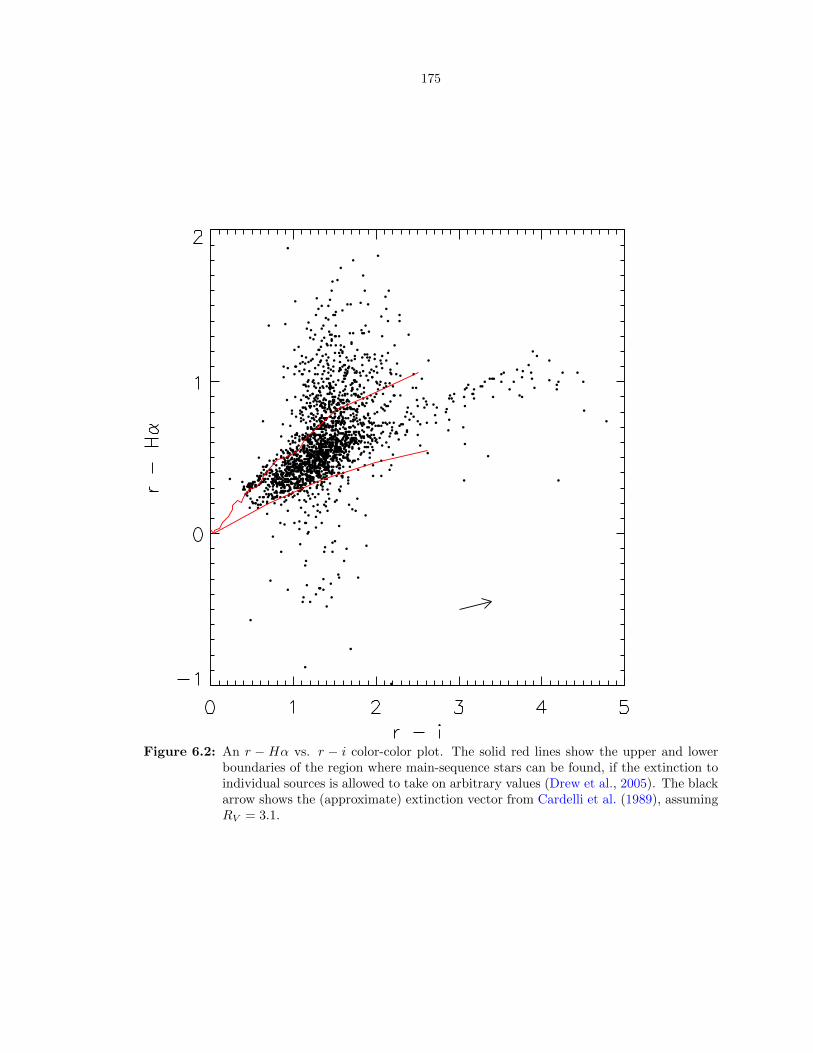
175

Figure 6.2: An r − Hα vs. r − i color-color plot. The solid red lines show the upper and lowerboundaries of the region where main-sequence stars can be found, if the extinction toindividual sources is allowed to take on arbitrary values (Drew et al., 2005). The blackarrow shows the (approximate) extinction vector from Cardelli et al. (1989), assumingRV = 3.1.

176

(a) All variables (b) Spectroscopic targets only

Figure 6.3: An i vs. r−i color-magnitude plot. The red curves show, from top to bottom, syntheticphotometry of D’Antona & Mazzitelli (1997) isochrones at 1 Myr, 3 Myr, and 10 Myrat a distance of 600 pc. The blue curve is the empirical main sequence from Kraus &Hillenbrand (2007) at the same distance. The black arrow shows the extinction vectorfrom Cardelli et al. (1989), assuming RV = 3.1. Extinction tends to shift sources ontoyounger isochrones. In the right panel, red triangles are high-confidence members, bluesquares low-confidence members, and black squares likely non-members, as defined insubsection 6.4.2. Very red sources r− i & 1 tend to be much more luminous than othersources in the field, indicating that they are background giants.

throughout the rest of this chapter to allow for a more conservative rejection of background sources.

The reddening vector tends to raise sources above the main sequence, so any sources below it should

be non-members with high probability, regardless of their extinction.

Since many IPHAS sources in the region have i photometry but not r, and cannot be placed

on the color-magnitude diagram directly, we also reject sources with i > 18.7. Sources that have

i > 18.7 but fall within our detection limit of RPTF ≤ 20 are assumed too blue to fall above the

main sequence, although we caution that the IPHAS i photometry is unlikely to have been taken

while the source was near its median PTF magnitude.

There are five sources that are well below the main sequence line, yet are high-confidence spec-

troscopic members. These sources are:

FHO 89 (i = 18.0, r − i = 1.41) The IPHAS r magnitude of 19.4 is considerably fainter than the

observed range RPTF ∼ 17.7-18.4. However, this source is clearly blended in the PTF image,

so likely neither the IPHAS nor PTF photometry are reliable.

FHO 299 (i = 18.4, r − i = 1.53) is a source with a 3-magnitude peak-to-peak amplitude that

appears to have been observed by IPHAS close to minimum light. The source would spend

most of its time above our background source cutoff.

177

FHO 558 (i = 13.7, r−i = 0.23) is V751 Cyg, a known cataclysmic variable. This source illustrates

that even high-confidence members are not necessarily young stars.

FHO 568 (i = 18.5, r − i = 1.48) The IPHAS r magnitude of 20.0 is considerably fainter than the

observed range RPTF ∼ 17.3-18.7. However, this source is a close double in SDSS images, so

likely neither the IPHAS nor PTF photometry are reliable.

FHO 1891 (i = 17.0, r − i = 0.93) is a young star with both a strong emission-line spectrum

and a strong infrared excess. Variability cannot account for its position in the IPHAS color-

magnitude diagram.

Of the five sources, then, only two, FHO 299 and FHO 1891, represent high-quality detections

of young stars. This supports the idea that most of the sources below the blue line in Figure 6.3

are likely non-members. Therefore, we can remove sources below the main sequence line from our

sample without significantly sacrificing completeness.

Of 2,705 variable sources with good PTF photometry, 1,822 are sufficiently bright (above the

main sequence line) to be plausible members of the North America Nebula complex. Of those, we

exclude the 68 sources in the region with r − i > 2 and i < 10 + 2(r − i), including 24 of the 33

sources where we could rule out an infrared excess, as probable giants. This leaves 1,754 variables

with photometry consistent with North America Nebula membership.

6.4.5 Variability as a Youth Indicator

In Figure 6.4, I show the RMS amplitudes for sources whose spectra were examined for youth

indicators, according to their membership confidence. Here, and throughout the chapter, I use the

observed RMS of the lightcurve, rather than the RMS in excess of that expected from the source

magnitude as in Figure 3.1. The problem of correcting the RMS amplitude of a signal for a fixed

noise contribution is ill-posed: the relationship between signal RMS, noise RMS, and combined RMS

depends on the distribution of both signal and noise; in addition, the simplest solution (subtraction

of the noise estimate in quadrature) carries the risk of returning imaginary results. I choose to use

the observed RMS, which is a well-understood quantity despite its magnitude dependence.

While high-confidence members to tend to have higher RMS than low-confidence or likely non-

members, there is still heavy overlap among the samples: RMS, taken by itself, cannot be used

to select members. This is consistent with the results of the spectroscopic analysis, which showed

that half our sample, selected by a combination of variability and infrared excess, had no youth

indicators. We may be able to revisit variability amplitude as a selection criteria once we are certain

which high-confidence members are genuine members and which likely non-members are genuine

non-members.

178

(a) High-Confidence Members (b) Low-Confidence Members

(c) Likely Non-Members

Figure 6.4: RMS vs. magnitude distributions for sources with different degrees of membershipconfidence. High-confidence members have slightly higher RMS amplitudes than othersources, but otherwise there is no correlation with the sources’ spectroscopic properties.The lower density of sources for 18 ≤ RPTF ≤ 18.5 is an artifact of us primarilychoosing sources brighter than 18th magnitude as spectroscopic targets.

179

Category Number NotesPrevious candidates from Rebull et al. (2011) 2,082Rebull et al. candidates detected by PTF pipeline 588 28% of candidatesRebull et al. candidates with reliable photometry 354 60% of PTF sourcesRebull et al. candidates recovered as variable sources 177 50% of reliable lightcurvesRebull et al. candidates rejected as members based on our spectra 6New variability-selected candidates 1,359New candidates with Spitzer counterpart 1,173 86% of candidatesCandidates with IPHAS r and i 897 76% of Spitzer sourcesNew candidates with high-confidence membership spectrum 54New candidates with low-confidence membership spectrum 128New candidates with no spectrum 1,177 87% of new variable candidates

Table 6.1: Summary statistics for our sample of 3,441 candidate members, including candidatesfirst identified here and candidates selected by Rebull et al. (2011). Only PTF sourceson the westernmost 6 chips of the field are considered. “Reliable photometry” is definedas 13.5 ≤ RPTF ≤ 20.0 and unflagged observations in at least half of all epochs.

Given the probable high contamination of a variability selected-sample, section 6.5 and later will

focus on the 282 spectroscopic candidate members except where otherwise stated.

6.4.6 New Candidate Members in the North America Nebula Complex

Our final membership list is based on a large number of partially overlapping samples. In addition to

the infrared-excess selected list of Rebull et al. (2011), we have Spitzer photometry for many other

sources in the field. We have the PTF source catalog for our field, including sources that appear to

be variable. We have follow-up spectra of a subset of the infrared-excess sources and the variables,

and we have IPHAS photometry for a subset of the Spitzer sources, both with and without infrared

excess.

We begin with the list of 2,082 candidate members from Rebull et al. (2011), of which only 629

are optically visible according to IPHAS. To this list, we add the sources we selected in this section on

the basis of optical variability and follow-up spectroscopy. These two samples are complementary:

the Rebull et al. (2011) sources are dominated by infrared excess sources, while our variability-

selected sample is more sensitive to sources with little to no infrared excess. We define a source as a

candidate member of the North America Nebula complex if it was identified as a candidate member

by Rebull et al. (2011), or if it meets all of the following criteria:

1. it is variable

2. it does not have a spectrum indicating likely non-membership

3. it either has a position in the IPHAS color-magnitude diagram consistent with membership or

is missing IPHAS photometry

These criteria produce a list of 3,441 candidate members, 1,359 of them not selected by Rebull

et al. (2011), which are listed in Table 6.2. Some more details of the candidate selection are listed in

Table 6.1. The variability selected candidates overlap only slightly with the infrared excess selected

180

[RGS2011] ID FHO Rmed RMS [RGS 2011] Spectroscopic PhotometricNumber (mag) (mag) Class Membership Membership

205009.17+445518.7 31 17.7 0.17 Possible Member205011.62+445522.7 33 18.9 0.28205015.00+441741.9 34 19.3 0.35205018.20+440402.2 39 18.0 0.15 Possible Possible Member205019.86+440221.2 40 17.1 0.09 Likely Possible Member

Table 6.2: All 3,441 candidate members identified by this study. Only a portion of the table isshown for reference; all 3,441 rows may be downloaded online. Rmed is the medianPTF magnitude of the lightcurve. RMS denotes the root-mean-square scatter ofthe lightcurve. The [RGS 2011] Class is the spectral class (I, flat, II, or III) assignedby Rebull et al. (2011). Spectroscopic membership is “Likely” for high-confidencemembers, “Possible” for low-confidence members, and “Non-Member” for likelynon-members. Photometric membership is “Background” for sources that fell belowthe main sequence in Figure 6.3, “Giant” for sources that are likely giants, and“Possible Member” for sources whose color-magnitude diagram position is consistentwith North America Nebula Complex membership.

candidates of Rebull et al. (2011); only 154 out of the 3,441 candidate members were selected by

both methods. Some of the limited overlap can be attributed to the different wavelength regimes

probed by PTF and Spitzer: while 88% of the PTF-selected candidates are detected by Spitzer, only

17% of the Spitzer-selected candidates fall in the PTF photometric sample.

Many of the 1,359 new variability-selected candidates have neither sufficient optical photometry

to place them on an i vs. r − i color-magnitude diagram, nor a spectrum to test their membership.

Therefore, it is likely that some will be classified as likely non-members on further investigation. We

can obtain a rough estimate of the number of members that will remain by examining the source

statistics. Of the 398 sources with a good position in the color-magnitude diagram and a spectrum

available, 171 (43%) show youth indicators in their spectrum. Of the 23 sources with no color-

magnitude information but a spectrum available, 11 (48%) show youth indicators. Of the 202 sources

with color-magnitude information and a spectrum consistent with youth, 171 (85%) have a CMD

position consistent with membership. Of the 1,463 sources with color-magnitude information but no

spectrum, 726 (50%) have a CMD position consistent with membership. Of the 1,359 new candidates,

171 have both a spectrum and a CMD position available, 11 have only a spectrum, 726 have only a

CMD position, and 451 have neither a spectrum nor a CMD position. Assuming for simplicity that

there are no biases between the samples with and without CMD or spectrum information, the number

of sources that are expected to remain in the sample of new candidates after obtaining photometry

and spectra for all variable sources is 171+11×0.85+726×0.43+451×(0.43×0.50 OR 0.85×0.48),

for a total of 590-680 vetted candidates, depending on the highly uncertain confirmation rate for the

451 sources with no supplementary data.

Therefore, our catalog of 3,441 candidate members is expected to correspond to an expected pop-

ulation of 2,600-2,700 likely members after additional followup work. This is a significant expansion

over the ∼ 2, 000 sources associated with the region by Rebull et al. (2011). In addition, since our

181

variability survey is amplitude limited (as discussed in subsection 6.6.1, particularly Figure 6.13),

it is likely that improvements to the PTF pipeline that lower our detection thresholds will uncover

additional candidates.

6.5 Applying Timescale Metrics

6.5.1 Characterizing the Full Variability-Selected Sample of NAN Can-

didate Members

For each of the 2,705 variables in the PTF sample, I calculated the ∆m-∆t plot with ∆t bins in

steps of 0.15 dex from 10−1.97 days to the maximum length of the lightcurve. This is the same

binning used in Chapter 5 when testing the performance of ∆m-∆t plots; while somewhat coarse,

it ensures a statistically significant number of points in most bins, and allows the coverage gap at

time intervals of 8-16 hours to be isolated to just two bins, from 10−0.43 days to 10−0.17 days.

The two ∆t bins on either side of this gap will be well-populated by intranight observations

on the short end and by observations on consecutive nights on the long end. The clean contrast

minimizes systematic errors: the two undersampled bins from 10−0.47 days to 10−0.17 days have

very few points “spilling over” from adjacent, better-populated, bins, while the adjacent bins have a

roughly uniform sampling across their ∆t width. As an additional safeguard, we ignored the small

number of points falling within the two undersampled bins from 10−0.47 days to 10−0.17 days.

For each ∆m-∆t plot, the ∆t bin in which the 90th percentile of ∆m first exceeded half the

lightcurve amplitude was defined as the timescale of the lightcurve, as the simulations summarized

in section 5.9 show this timescale metric performs well in the parameter space occupied by the

PTF North America Nebula survey. Timescales were calculated both by considering all points in

the lightcurve and by considering only points with photometric errors smaller than 0.1 mag. A

comparison is shown in Figure 6.5. It is more common for a timescale with high-error points to be

less than the corresponding timescale without those points than for the reverse to be true, which is

consistent with expectations if the timescale is biased downward by noisy points. Deviations between

the two measurements are most common if at least one timescale is shorter than 0.1 day.

A large fraction of our sources are aperiodic, and characterizing these sources is a major goal

of our survey. Therefore, the most relevant simulations from Chapter 5 are those for a squared

exponential Gaussian process and for a damped random walk. In Figure 5.11, these simulations

typically have timescales characterized to 20-50%, depending on the choice of lightcurve model and

on the value of the timescale. Since, as shown in the next section, many lightcurves have timescales

of order a day but complex structures more similar to a damped random walk than to a squared

exponential Gaussian process, I adopt 50% as the typical timescale uncertainty in this sample.

182

Figure 6.5: Timescales for variable PTF sources calculated including (vertical axis) and ignoring(horizontal axis) points with photometric errors exceeding 0.1 mag. Only the 1,845sources for which both timescales could be calculated are shown. Timescales have beenrandomized by ±0.05 dex to clarify the number of points in each bin. The gap at ∼ 0.5days is imposed by our nightly cadence. For most sources, the two timescales fall inthe same bin, or differ by at most one bin.

183

Inspection of sources with timescales shorter than 0.1 day reveals no single cause for the short

values. Some lightcurves appear to simply be noisier than the majority of stars with the same

median magnitude, leading to their false classification as variables on the basis of their RMS. Some

lightcurves have unflagged artifacts in the photometry, particularly blended sources or bad CCD

columns. Others are lightcurves with 0.1-0.2 day variability that fell below 0.1 day due to timescale

uncertainty.

In the remainder of this chapter I use timescales excluding points with 0.1 mag or larger errors,

and discard values below 0.1 day as invalid. This leaves 515 sources with timescale measurements,

207 of which have spectra.

6.5.2 Timescales in the North America Nebula Complex

The ∆m-∆t plots for the 2,705 PTF variables show a wide variety of behaviors. I show some typical

examples of high-confidence candidates in Figure 6.6, low-confidence candidates in Figure 6.7, and

likely non-members in Figure 6.8. As these figures show, ∆m-∆t plots provide information about

lightcurve structure regardless of magnitude, noise level, and membership probability.

As a further illustration, Figure 6.9 shows examples as a function of timescale across two and a

half orders of magnitude. The timescale definition adopted in subsection 6.5.1 represents the time

one must wait to see a large change in magnitude, relative to the overall lightcurve amplitude. For

periodic sources, for example, the timescale as defined here should never exceed half the period and

may be considerably shorter, depending on the shape of the lightcurve.

While we cannot directly measure the amount of variability occurring in the nightly gap at

10−0.47-10−0.17 days, the ∆m-∆t plots suggest that this is an important time interval to characterize.

Many sources have significantly higher ∆m values in the 10−0.17-10−0.02 day bin than in the 10−0.62-

10−0.47 day bin, suggesting that you can see significant changes on time intervals of less than a day.

This does not appear to be a bias related to the one-day average cadence, as the simulations of

Chapter 5 showed no predisposition for the 10−0.17-10−0.02 day bin to be substantially higher than

the 10−0.62-10−0.47 day bin. Time intervals in the nightly gap have been probed by Cody et al. (2013)

and Cody et al. (2014) using space-based data, but the lightcurves illustrated in either publication

show relatively little variation over time intervals of less than a day. A more thorough statistical

analysis will be published at a later date.

Some lightcurves also show substantial variation on time intervals of 0.1 day or less. In Fig-

ures 6.6b, 6.7b, and 6.8c, a smaller fraction of point pairs show a large magnitude change at short time

intervals than at long ones; this can be seen from the coloring of the low-amplitude (∆m . 0.1 mag)

bins in those plots, which contain most of the sources at short time intervals but not at long ones.

For these, the short timescale is somewhat misleading, and choosing a lower percentile than the 90th

as the basis of the timescale should raise the result. In Figures 6.8a, 6.8h, 6.8e, and 6.8i, on the other

184

(a) FHO 1223, RPTF = 15.4,σR = 0.30, τ = 0.5 days

(b) FHO 164, RPTF = 16.4,σR = 0.34, τ = 0.02 days

(c) FHO 588, RPTF = 17.4,σR = 0.32, τ = 0.7 days

(d) FHO 112, RPTF = 14.6,σR = 0.13, τ = 2 days

(e) FHO 25, RPTF = 16.0,σR = 0.13, τ = 5 days

(f) FHO 1089, RPTF = 18.2,σR = 0.34, τ = 11 days

(g) FHO 103, RPTF = 14.0,σR = 0.05, τ = 0.02 days

(h) FHO 420, RPTF = 16.3,σR = 0.09, τ = 0.5 days

(i) FHO 4, RPTF = 17.6,σR = 0.14, τ = 2 days

Figure 6.6: Typical ∆m-∆t examples for high-confidence candidates, showing that ∆m-∆t plotswork at all magnitudes, noise levels, and amplitudes. Sources get fainter moving fromleft to right, and lower-amplitude (relative to the noise level, see subsection 3.2.1)moving from top to bottom. Light shading indicates a high fraction of points in a ∆tbin (column) fall in a particular cell; dark shading indicates a sparsely populated cell.Red lines are, from top to bottom, the 90th, 50th, and 10th percentiles of ∆m in each∆t column. A variety of timescales are represented, from 0.02 days (Figure 6.6b) to11 days (Figure 6.6f).

185

(a) FHO 585, RPTF = 15.4,σR = 0.19, τ = 5 days

(b) FHO 81, RPTF = 15.8,σR = 0.24, τ = 1.0 days


(d) FHO 98, RPTF = 14.5,σR = 0.10, τ = 0.02 days

(e) FHO 465, RPTF = 16.8,σR = 0.11, τ = 0.04 days

(f) FHO 881, RPTF = 17.9,σR = 0.19, τ = 0.03 days

(g) FHO 1814, RPTF = 14.6,σR = 0.05, τ = 2 days


(i) FHO 743, RPTF = 17.8,σR = 0.13, τ = 0.011 days

Figure 6.7: As Figure 6.6, but for low-confidence candidates. Timescales range from 0.011 days(Figures 6.7h and 6.7i) to 5 days (Figure 6.7a).

186

(a) FHO 2133, RPTF = 15.0,σR = 0.27, τ = 0.03 days

(b) FHO 1467, RPTF = 15.9,σR = 0.21, τ = 20 days


(d) FHO 470, RPTF = 14.6,σR = 0.10, τ = 15 days

(e) FHO 2170, RPTF = 16.0,σR = 0.10, τ = 0.06 days

(f) FHO 1572, RPTF = 17.2,σR = 0.15, τ = 0.02 days

(g) FHO 1952, RPTF = 14.8,σR = 0.06, τ = 2 days


(i) FHO 830, RPTF = 18.1,σR = 0.17, τ = 0.02 days

Figure 6.8: As Figure 6.6, but for likely non-members. Timescales range from 0.02 days (Fig-ures 6.8a, 6.8c, and 6.8h) to 20 days (Figure 6.8b).

187

(a) FHO 827, τ = 0.3 days (b) FHO 13, τ = 1.3 days

(c) FHO 1039, τ = 15 days (d) FHO 2175, τ = 85 days

Figure 6.9: Typical ∆m-∆t examples for high-amplitude sources at a variety of timescales. Lightshading indicates a high fraction of points in a ∆t bin (column) fall in a particular cell;dark shading indicates a sparsely populated cell. Red lines are, from top to bottom,the 90th, 50th, and 10th percentiles of ∆m in each ∆t column.

188

hand, the ∆m distribution seems to be nearly independent of the time interval on which observations

are compared. At face value, this distribution means that the source experiences 0.2 mag or greater

changes in 30 minutes or less, but no additional variability at longer time intervals; inspection of

the lightcurves confirms that they show no correlation even in high cadence data. While we find

it implausible that a star would have such rapid and short timescale variability, we cannot find a

specific systematic error affecting these stars but not others. Any conclusions regarding variability

on very short timescales will require further study.

The distribution of timescales is shown in Figure 6.10. Values range from our cutoff at 0.1 days to

timescales just over 100 days, where simulations show that ∆m-∆t timescales have an average ceiling

set by our observing cadence (see Figure 5.12 and accompanying text). The 10−0.17-10−0.02 day bin

has a disproportionately large number of sources, because it includes sources whose true timescale

would lie within the poorly sampled gap at ∼ 0.5 days: in effect, the bin contains sources with a

timescale anywhere between 10−0.47 days and 10−0.02 days.

Even ignoring the inflated 10−0.17-10−0.02 day bin, the timescale distributions for all sources and

for high-confidence members are inconsistent with a log-uniform distribution over [1, 100], with a

two-sided Kolmogorov-Smirnov (K-S) test returning a p-value smaller than 2× 10−16 for all sources

and a p-value of 8×10−14 for high-confidence members. The plot for high-confidence members shows

a pronounced excess of sources with characteristic timescales between 1 day and 2 days, separate

from the artificially enhanced 10−0.17-10−0.02 day bin. We see no tendency for ∆m-∆t timescales

to cluster between 1 day and 2 days in the simulations of Chapter 5, so this is unlikely to be a

systematic effect related to either the cadence or the ∆m-∆t method.

This result is broadly consistent with previous results finding periods of order a week for period-

ically varying young stars. According to Table 4.3, the characteristic timescale of a sinusoidal signal

should be 1/6 its period. The periods for T Tauri stars are typically in the 2-15 day range, peaking

at 6-8 days (Herbst et al., 2000; Cohen et al., 2004); any periodic T Tauri stars in our sample should

therefore either be part of the ∼ 1 day peak or fall in our ∼ 0.5 day gap.

With a K-S p-value of 0.009, the timescale distribution for low-confidence members is marginally

inconsistent with a log-uniform distribution; there are hints that it may also have a peak at 1-2 days.

The timescale distribution for likely nonmembers, on the other hand, is marginally consistent with

a log-uniform distribution, with a p-value of 0.02. However, since these samples have only 26 and 17

sources, respectively, with timescales of 1 day or longer, any tests of their distributions are necessarily

imprecise.

The timescale distribution with magnitude is shown in Figure 6.11. There is no change in the

measured timescales with respect to magnitude. This suggests that the same timescales are relevant

for high- and low-luminosity sources (with the important caveat that only some variables are North

America Nebula members, and therefore at the same distance), and reassures us that timescales

189

(a) All Sources (b) High-Confidence Members

(c) Low-Confidence Members (d) Likely Non-Members

Figure 6.10: Distribution of timescales for all sources, whether or not they have a spectrum, andfor high-confidence members, low-confidence members, and likely non-members, asdefined in subsection 6.4.2. High-confidence members are likely to have timescalesaround ∼ 1 day, while both low-confidence members and likely non-members have aflat timescale distribution to within the limitations of the small number statistics.

190

Figure 6.11: The distribution of timescales as a function of median PTF magnitude. There is littleto no correlation between timescale and magnitude; sources both bright and faint canhave any timescale in the sample.

for faint sources are not dominated by photometric noise, which would produce an excess of short

timescales.

The data set therefore contains aperiodic variability on timescales from just under a day to

the longest scales detectable with our data. There appears to be a large number of sources with

timescales of 1-2 days, consistent with variability from stellar rotation or dynamical changes at the

inner disk edge. We see a sharp increase in variability between the longest intranight time baselines

and the shortest baselines between consecutive nights, suggesting that variability on baselines of half

a day may be worth following up with more appropriate data sets.

6.6 Variability Properties

6.6.1 Timescales and Amplitudes

I show the distribution of timescales and amplitudes for all sources in the sample of 2,705 variables,

whether or not they had spectra, in Figure 6.12 and Figure 6.13, respectively. The two figures

divide sources according to the detection or non-detection of an infrared excess, as described in

subsection 6.4.3. The sources without a detected infrared excess are expected to be dominated by

sources that genuinely lack an excess above their photosphere, but many of these sources were also

too faint to be detected by Spitzer at 24 µm, so a weak long-wavelength excess cannot be ruled out.

191

(a) Infrared Excess (b) No Infrared Excess

Figure 6.12: Distribution of timescales for sources with and without an infrared excess. Sourceswith an infrared excess tend to cluster around timescales of ∼ 1-2 days.

The distribution of timescales for infrared excess sources, shown in Figure 6.12a, resembles

that for high-confidence spectroscopic candidates (Figure 6.10b), in that the distribution reaches a

maximum on timescales of 1-2 days. This is in large part due to the overlap between the samples: 78%

of infrared excess sources with spectra are high-confidence candidates, while 63% of high-confidence

candidates with a Spitzer counterpart have an infrared excess.

The distribution for sources that were not identified in subsection 6.4.3 as having an infrared

excess appears much flatter than that for infrared excess sources. Despite the apparent even distri-

bution, a two-sided Kolmogorov-Smirnov (K-S) test finds that the data for timescales longer than

1 day are inconsistent with a log-uniform distribution over [1, 100], with a p-value of 0.0003. The

current data suggest these sources have a slight preference towards timescales of 3-5 days, but a

larger sample will be needed to confirm.

The amplitude distributions in Figure 6.13 for sources with and without a detected infrared

excess are similar to each other, except that the infrared excess sources tend to have slightly higher

amplitudes on average as well as a longer tail to high amplitudes. The differences between the two

samples are significant; a two-sided Kolmogorov-Smirnov test comparing the two samples finds a

p-value of 2× 10−5.

Both distributions peak at around 0.1-0.2 mag, somewhat higher than our detection threshold of

0.07-0.1 mag (see Figure 3.1 for detection thresholds as a function of chip and magnitude). Because

192


Figure 6.13: Distribution of amplitudes for sources with and without a detected infrared excess.The distribution for infrared excess sources is somewhat broader, and both rise up-ward to our detection threshold at ∼ 0.1 mag.

our survey is amplitude-limited, the similarity in peaks does not necessarily indicate a similarity

between the infrared-excess and non-infrared-excess sources; we may merely be probing the high-

amplitude tail of either distribution.

The joint distribution of timescale and amplitude is shown in Figure 6.14. Many of the results

from Figure 6.12 and Figure 6.13 can be seen here, including the concentration of sources toward

short timescales and the scarcity of sources with higher RMS amplitudes than 0.5 mag.

The most striking property of the joint distribution of timescale and amplitude is that there is

no strong trend between amplitude and timescale. Sources below 0.4-0.5 mag may have almost any

combination of amplitude and timescale. In particular, we see a handful of sources with timescales

of ∼ 100 days, but amplitudes of only ∼ 0.1 mag; to our knowledge, this is the first time that

low-amplitude, long-timescale variability has been identified. Sources above 0.5 mag are too sparse

to constrain the timescale distribution.

6.6.2 High-Amplitude Sources

We individually examined the lightcurves and spectra of all candidate members with RMS amplitudes

exceeding 0.6 mag. Of 17 sources with high amplitudes, four (FHO 222, FHO 1176, FHO 1346, and

FHO 1951) have pulsating lightcurves, and of those FHO 1176 and FHO 1346 also have spectra

193


Figure 6.14: RMS vs. timescale distributions for sources with and without a detected infraredexcess from subsection 6.4.3. Timescales have been randomized by ±0.05 dex forclarity. While sources with infrared excess tend to have slightly higher amplitudesand timescales around ∼ 1 day, there are few clear groups within the amplitude-time parameter space. Sources above 0.6 mag RMS marked by red boxes are giants,while those marked by X’s are dominated by pipeline problems; see subsection 6.6.2for more details. Sources above 0.6 mag that are not marked appear to be genuineyoung stars on closer inspection.

194

consistent with late-type stars. We believe these four sources to be background giants; none have

IPHAS photometry, and they could not be rejected using a color-magnitude diagram. Another six

sources (FHO 180, FHO 232, FHO 444, FHO 1351, FHO 1518, and FHO 2348) have no apparent

structure in the lightcurve or have obvious unflagged artifacts.

The remaining seven (FHO 105, FHO 455, FHO 561, FHO 598, FHO 618, FHO 781, and

FHO 2359) appear to be genuine high-amplitude variables that do not behave like giants. Of the

seven, all except FHO 618 have a detected infrared excess, and all except FHO 598 and FHO 2359

have spectra (all of which show youth indicators).

While there is some giant contamination in our sample, a large number of sources appear to be

genuine young stars. We mark giants in Figure 6.14 with boxes, and stars with suspect photometry

with crosses. Unmarked high-amplitude sources in Figure 6.14 are likely candidate members.

6.6.3 Correlation with Infrared and Emission Line Properties

The amplitude and timescale for all 2,705 PTF variables is plotted against 2MASS/Spitzer infrared

color in Figure 6.15. Point colors indicate the infrared source class from Rebull et al. (2011); black

points are sources that either had insufficient photometric data for Rebull et al. to classify, or, on

the left side of either panel, that were not found to have an infrared excess by Guieu et al. (2009)

or Rebull et al. (2011).

The black curve in either panel shows the median K − [8.0] color for stars of a given amplitude

or timescale. Variables with RMS amplitudes below 0.3 mag are predominantly sources with blue

infrared colors, which may or may not be young stars; the majority of variables with amplitudes

above 0.3 mag have a clear excess. A majority of variables with timescales between 0.7 days and

6 days have an infrared excess, while most variables with either longer or shorter timescales do not.

There is a hint that variables with timescales of ∼ 80 days or longer are also predominantly infrared

excess sources, but more examples of long-timescale variables will be needed to confirm this.

The variability properties of the sources with spectra are shown in Figures 6.16 and 6.17 as a

function of the equivalent widths of the Hα 6563 A, Ca II 8542 A, and Li I 6708 A lines. Hα and

Ca II are both accretion indicators, and show similar behavior in both figures. The strongest Hα and

Ca II emitters have amplitudes of 0.4-0.5 mag, and the strongest Hα emitters also have timescales of

0.7-1 days. The strongest Ca II emitters show no preference for a particular timescale. For weaker

emitters, there seems to be no trend between either Hα or Ca II strength and timescale.

The highest-amplitude sources in Figure 6.16 tend to be only modest Hα and Ca II emitters,

with Hα equivalent widths of a few tens of A and Ca II widths of around 10 A. While line equivalent

width is only a crude measure of accretion rate, these results suggest that the highest-amplitude

variables may not be (directly) accretion-powered. A comparison with accretion rate measurements

for these stars may clarify these results.

195

Figure 6.15: Optical lightcurve properties as a function of infrared class and color for variablePTF sources whose lightcurves have flags (listed in subsection 2.2.2) in fewer thanhalf the epochs. Both amplitude and timescale are weakly correlated with the source’sinfrared properties; one can find a range of colors at any amplitude or timescale and arange of amplitudes and timescales at any color. Timescales have been randomized by±0.05 dex for clarity. The solid line indicates the median color in 15-point bins (left)or in the ∆t bins used for the ∆m-∆t plot (right). The color of the dots indicates thedegree of infrared excess: blue dots are class III sources, green ones class II, yellowones have a flat IR spectrum, while magenta sources are class I sources. Black sourceswere not assigned an IR excess class by Rebull et al. (2011), either because they didnot have an excess or because they were too faint to classify definitively.

196

Figure 6.16: The variability amplitude vs. the strength of the Hα 6563 A and Ca II 8542 Alines, which probe accretion onto the star, and Li I 6708 A, which probes stellar age.Strong Hα and Ca II emitters, and presumably rapidly accreting stars, do not havethe highest amplitudes, but strong Li I absorbers, presumably the youngest stars, do.

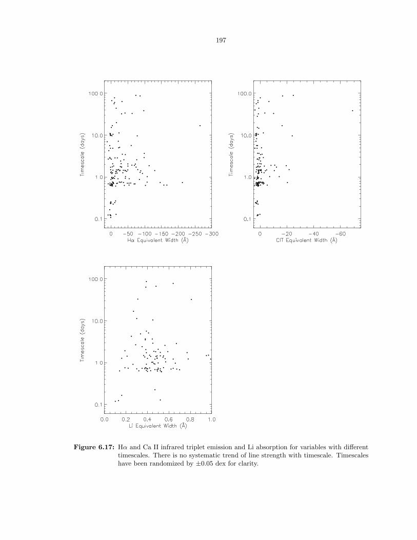
197

Figure 6.17: Hα and Ca II infrared triplet emission and Li absorption for variables with differenttimescales. There is no systematic trend of line strength with timescale. Timescaleshave been randomized by ±0.05 dex for clarity.

198

While there is no significant correlation between variability amplitude and Li I equivalent width

in Figure 6.16, we do find that the two highest-amplitude sources with lithium measurements also

have among the strongest equivalent widths. Two sources are not, however, statistically significant.

While stars with Li I equivalent widths exceeding 0.3 A appear to have no preference for timescale

in Figure 6.16, stars with weaker lithium detections tend to have short timescales. It is not clear

whether this is a genuine trend in stellar properties, or whether we are insensitive to weak lithium

lines in longer-term variables. Long-term variables are no more likely to be faint than short-term

variables (Figure 6.11), so this is not simply a matter of long-term variables having noisier spectra.

Figure 6.18: Distribution of amplitudes and timescales for sources with lithium absorption. Aswith the infrared excess sources, timescales tend to cluster around timescales of ∼1 day. Only stars with lithium detections are shown, so the plot is incomplete, andin particular biased toward sources with low veiling — only 45% of variable sourceswith an infrared excess show detectable lithium absorption.

In Figure 6.18, I show the amplitude and timescale distributions of all sources with Li I detections,

regardless of the strength of the line. These distributions closely resemble those for high-confidence

members (Figure 6.10b; all lithium sources are high-confidence members by definition, while 82%

of high-confidence members have lithium detections) and infrared excess sources (Figure 6.13a and

Figure 6.12a; 63% of all lithium sources have an infrared excess, while 73% of all infrared excess

sources with spectra have detectable lithium absorption).

There appears to be no strong correlation between variability timescale and infrared color, emis-

sion line equivalent width, or lithium absorption equivalent width. The lack of a correlation suggests

199

that neither short- nor long-term variables represent a homogeneous group, but instead probe a

blend of all physical mechanisms consistent with that timescale. We discuss the breadth of such

mechanisms in the following section.

6.6.4 Evidence for Multiple Dominant Variability Mechanisms

As discussed in subsection 1.2.1, the timescale of a young star’s variability should be tied to the

region of the star or circumstellar environment responsible for the variability. The only processes

that should be able to produce variability on timescales of hours are inside the inner disk edge, for

example in funnel flows. Changes on the order of days can be caused by dynamical processes at the

inner edge of the disk or by rotation of the star. Timescales on the order of weeks may be associated

with changes in the stellar magnetosphere, or with phenomena in the inner disk beyond the disk

edge, while timescales of months or years may be probed by dynamical processes farther out, or by

viscous processes at the disk edge. On timescales of years, stellar activity cycles may also come into

play.

Many of the infrared excess sources change brightness significantly within one or two days,

consistent with previous observations and with expectations that the variability should be associated

with stellar rotation or with processes at the inner disk edge. However, the presence of both high-

and low-amplitude variability on timescales from ∼ 0.7 days to ∼ 100 days suggests that we are

seeing a variety of physical processes in the disk, not merely dynamical changes at the disk rim.

Figure 6.14a may be used to select targets dominated by particular variability mechanisms; for

example, large-amplitude variations on timescales of months may correspond to large accretion or

extinction events in the inner disk.

However, we also see variations on timescales of up to several months in sources that do not

have a detected circumstellar disk. Of the 23 candidate members with no detected infrared excess

and a timescale above 20 days, 11 can be placed on Figure 6.2, where their colors and magnitudes

are inconsistent with being giants. Some of these sources appear to be unflagged systematics in

the photometry. Some (FHO 2084, FHO 2402) show signs of accretion, and may have a very

weak, undetected infrared excess. Others (FHO 755, FHO 1574) show irregular variability typically

associated with young stars, but do not yet have spectra we can use to constrain the presence or

absence of accretion. It is possible that these are diskless members of the North America Nebula

complex, and that an unforeseen mechanism is responsible for the variability. Future spectroscopy

will determine if this is the case.

200

6.7 Discussion

6.7.1 Comparison with Other State-of-the-Art Data Sets

6.7.1.1 Peak-Finding Timescales from CSI 2264

The CSI 2264 survey (Stauffer et al., 2014) of the NGC 2264 region combined infrared time se-

ries photometry from Spitzer with optical time series photometry from CoRoT to investigate the

variability of young stars in both wavelength regimes. Cody et al. (2014) calculated timescales for

CoRoT lightcurves from the survey using the peak-finding method, which we described in section 5.6

and illustrated in Figure 5.13. Since their lightcurves covered an interval of 39 days at a roughly

10 minute cadence, the optical data set of Cody et al. (2014) is complementary to ours, probing

shorter timescales than is practical with PTF.

Because peak-finding uses a different definition of timescale than ∆m-∆t plots do, care must be

taken when comparing our results to those of Cody et al. (2014). We have carried out simulations

similar to those presented in section 5.6 for the cadence used by CSI 2264, at a signal-to-noise ratio

of 100, a value typical of the lightcurves studied by Cody et al.. In these simulations we defined the

peak-finding timescale to be the timescale of variations 80% as tall as the tip of the peak-finding

curve, like Cody et al. did.

We present the simulation results in Figure 6.19. The top row of panels, which compares the

timescale found by peak-finding to the timescale parameter used in the simulations, show that the

peak-finding timescale is proportional to the timescale input to the simulation (the “true timescale”)

for true timescales between 0.1 and 10 days. For longer-term variables, the timescale from the peak-

finding analysis appears to level out at roughly 20 days. The middle row of panels shows that, for

aperiodic signals, the scatter in timescales is of the same order as the timescale itself, or a factor of

two error. This is comparable scatter to that found in Chapter 5 for both peak-finding and ∆m-∆t

plots run on the PTF cadence.

Cody et al. (2014) normalized their peak-finding timescale to twice the value used in Table 5.5 or

plotted in Figure 6.19 so that it would agree with the period for periodic sources. After we correct for

this convention, introduced after the simulations were carried out, our simulations indeed show that

the peak-finding timescale found for simulated sinusoidal signals equals the period on average. Mul-

tiplying the peak-finding rows of Table 5.5 by two, we find that timescales computed by peak-finding

for CSI 2264 lightcurves are expected to be 6-12 times larger than timescales computed from ∆m-∆t

timescales for PTF-NAN lightcurves, given the same underlying process for generating lightcurves.

The ratio between peak-finding and ∆m-∆t timescales depends on the statistical properties of the

lightcurve, and the figure of 6-12 times should be taken as representative values only. However, since

any individual measurement of either timescale metric may be uncertain by up to a factor of two,

201









Figure 6.19: The timescale calculated from a peak-finding plot in simulated CoRoT observations,plotted as a function of the underlying timescale of the simulated lightcurve. Toppanels show the average value of the output timescale, which increases linearly withthe true timescale before deviating from linearity at ∼ 10 days. Middle panels showthe ratio of the standard deviation to the mean output timescale; the uncertaintyis typically a factor of two for the two aperiodic models. Bottom panels show thedegree by which the input timescale has to change to significantly affect the outputtimescale. In all plots, blue represents lightcurves with an expected 5th to 9th per-centile amplitude of 0.5 mag, orange an amplitude of 0.25 mag, green an amplitudeof 0.1 mag, and black an amplitude of 0.01 mag. All runs have a signal-to-noise ratioof 100.

202

the variation in the conversion factor does not affect our comparisons.

Cody et al. (2014) find a distribution of timescales that is quite broad, from ∼ 4 days to 40 days.

This is equivalent to ∼ 0.4-6 days by our definition, corresponding to the broad peak seen in

Figure 6.12. Figure 6.12a shows a substantial decrease in the number of variables with timescales

from 2 days to 6 days; Figure 33 from Cody et al. (2014) shows no such trend between 15 days

and 40 days. It is possible that the number of sources they count having timescales between 20 and

40 days is being inflated by longer-term (e.g., 100 day) variables, as the authors note.

6.7.1.2 Hα Emission Timescales from LAMP

The LAMP survey (Costigan et al., 2012) and follow-up work (Costigan et al., 2014) carried out

time series spectroscopy of selected accreting pre-main-sequence stars on time intervals ranging from

minutes to weeks. They characterized the variability of the Hα emission line, expressing the Hα

equivalent widths in terms of accretion rates using empirical relations.

Figures A17 and A18 in Costigan et al. (2014) are analogous to our ∆m-∆t plots, only with

∆ log M in place of ∆m, while Figure 11 from Costigan et al. (2012) can be compared to the median

curves in our ∆m-∆t plots. The main difference between our figures and theirs is that the figures

of Costigan et al. (2014) show very few pairs of points with no change in Hα flux. The lack of

pairs of observations with similar measurements in the Costigan et al. data is likely an artifact of

their limited time sampling. Costigan et al. (2014) find that Hα flux differences rise from short

time intervals to time intervals of 2-3 days, and then remain constant at longer time intervals. Since

the definition of lightcurve timescale adopted in subsection 6.5.1 only requires that a ∆m quantile

exceed half the overall lightcurve amplitude, Costigan et al. (2014) observe accretion variability with

characteristic timescales of ∼ 1 day in our formalism. This is consistent with the 1-2 day peak we

find for infrared excess sources.

Costigan et al. (2014) find that Hα variability on time intervals of hours is rare, occurring in

roughly 10% of observations. Likewise, Cody et al. (2014) found that variability rarely has timescales

of less than 0.4 days (in our ∆m-∆t convention). Based on these two studies, it appears that we do

not miss important variability classes by ignoring hour-scale variability in our own survey.

6.7.2 Systematic Errors in Non-Coeval Studies

While valuable, time series data requires a considerable investment of observing time. Single-epoch

photometry in multiple bands will remain an important tool for characterizing young stars for

the foreseeable future. However, when photometry from different epochs is combined to estimate

source colors or SEDs, variability introduces a systematic error that (for aperiodic variability) grows

monotonically with the length of the time span separating the combined observations. With the

∆m-∆t data from the PTF-NAN survey, we can quantify this error for the first time.

203

More formally, let an observer have photometric measurements mi in bands Bi measured at

epochs ti. I assume that the observer does not have any constraints on the variability of the source,

other than that it is a young star, and possibly the presence or absence of an infrared excess. The

calculation of source colors or SEDs from such a data set implicitly assumes that the magnitudes m0

at some common epoch t0 (where the index 0 can be chosen arbitrarily without loss of generality)

equal the observed magnitudes mi. If ti 6= t0 and the source is variable, using mi as an estimator

introduces an error in m0, in addition to any (photometric) error in measuring mi.

Without prior knowledge of any systematic trends in source brightness, and without prior knowl-

edge of whether any of the observed magnitudes are unusually high or low, the expected value of

mi − m0 is zero. The variance in estimating m0 is therefore E((mi − m0)2). In the ∆m-∆t for-

malism, if ∆t = ti − t0, then this is E((∆m)2). This average needs to be taken over not only all

possible values of t0 and ti, but also over the distribution of variability properties in the sample.

The expectation value can be factored:

E((∆m)2) =∑

sources

∑obs

(∆m)2p(data, src)

=∑

sources

∑obs

(∆m)2p(data|src)p(src)

=1

N

∑sources

(∑obs

(∆m)2p(data|src)

)

=1

N

∑sources

E((∆m)2|src)

This is simply the average across the sample of the structure function E((∆m)2) for each source.

Taking the square root yields the error introduced in the estimation of the magnitude m0 at one

epoch using the magnitude mi at another.

In Figure 6.20 we show plots of the variability-induced error for all candidate members brighter

than RPTF = 18.5, as well as the subsets with and without a detected infrared excess. The restriction

to sources brighter than 18.5th magnitude is to prevent the high noise levels of faint sources from

washing out the signal. For infrared excess sources, an observation one night old constrains the

source’s current magnitude to ∼ 0.1 mag. If observations in different bands are taken two weeks

apart, on the other hand, the delay introduces an error of ∼ 0.2 mag in translating the data to a

common epoch. When combining data from different years, the error on colors or SEDs grows to

be a substantial ∼ 0.5 mag. SEDs published using such widely separated photometry should be

interpreted with great caution.

If a young star has little to no infrared excess, on the other hand, coeval photometry is much

less important. Measurements separated by long timescales show little more scatter than measure-

ments separated by short timescales. Readers should use caution when interpreting Figure 6.20c,

204

(a) All Candidates (b) Infrared Excess Detected

(c) No Infrared Excess Detected

Figure 6.20: The error introduced by using the magnitude at one epoch to estimate that at another,as a function of the time interval separating the two epochs. These calculationsassume no knowledge of either the amplitude or the timescale of the source. Resultsare shown for any young star, for stars known to have an infrared excess, and starsthat either are known to lack an infrared excess or that have strong limits on anyexcess.

205

however; sources reported to have significant variability over time intervals below ∼ 0.1 day may

have otherwise undetected photometric errors.

6.8 Summary

We have used the presence of variability, combined with ancillary data, to identify 1,359 new candi-

date members of the North America Nebula complex. From our current source statistics, we expect

that 600-700 of these candidates will survive vetting. These are candidates that could not have been

selected using either of the previous two methods, namely emission-line and infrared excess surveys,

and may represent a population of nonaccreting stars in the region.

We have used newly developed timescale metrics to characterize the timescales of aperiodic

variability among both the newly and the previously identified candidates for the first time. We

adopt a definition of timescale that tends to be shorter than both periods (e.g., Cohen et al., 2004)

and peak-finding timescales (Cody et al., 2014), so our results need to be converted to equivalent

peak-finding times or periods before they can be compared to timescales found in previous work.

The calculations of Chapter 4 and the simulations of Chapter 5 provide guidance on how to do

such conversions. The exact conversion factor depends on the shape and statistical properties of the

lightcurves in a given sample, but conversions good to within a factor of a few can be done without

making any assumptions about the lightcurves being studied.

We see a large number of variables whose magnitude changes significantly on time intervals of

1-2 days, and a broader distribution from just under a day to ∼ 100 days, the longest timescale

characterizable with our data. We do not see any evidence, based on the simulations of Chapter 5,

that this peak is a systematic effect. We interpret the 1-2 day peak as variability arising from stellar

rotation or dynamical changes at the inner disk edge, but note that a wide range of variability

mechanisms must be invoked to explain the full range of timescales. We see no correlation between

the timescale and variability amplitude, infrared colors, or spectroscopic properties of a source,

suggesting that the factors that determine a star’s variability properties are more complex than

assumed by us or by previous authors.

Since we see a sharp increase in variability between the longest intranight time baselines and

the shortest baselines between consecutive nights, we believe that many sources undergo important

changes on time intervals of a large fraction of a day. Variability on time intervals of half a day may

be worth investigating in CoRoT, LCOGT, or other appropriate data sets. In addition, only part of

our sample has had spectra taken or analyzed for youth indicators; expanding the set of analyzed

spectra will help refine our membership list and constrain some of the ambiguities in the preceding

discussion.

206

6.9 References

Cardelli, J. A., Clayton, G. C., & Mathis, J. S. 1989, ApJ, 345, 245


Cody, A. M., Tayar, J., Hillenbrand, L. A., Matthews, J. M., & Kallinger, T. 2013, AJ, 145, 79,

arXiv:1302.0018

Cohen, R. E., Herbst, W., & Williams, E. C. 2004, AJ, 127, 1602, arXiv:astro-ph/0312066

Costigan, G., Scholz, A., Stelzer, B., Ray, T., Vink, J. S., & Mohanty, S. 2012, MNRAS, 427, 1344,

arXiv:1209.0462

Costigan, G., Vink, J. S., Scholz, A., Ray, T., & Testi, L. 2014, MNRAS, 440, 3444, arXiv:1403.4088

D’Antona, F., & Mazzitelli, I. 1997, Mem. Soc. Astron. Italiana, 68, 807

Drew, J. E. et al. 2005, MNRAS, 362, 753, astro-ph/0506726

Gizis, J. E., Reid, I. N., & Hawley, S. L. 2002, AJ, 123, 3356, astro-ph/0203499

Gondoin, P. et al. 2012, A&A, 548, A15, arXiv:1210.3221

Guieu, S. et al. 2009, ApJ, 697, 787, arXiv:0904.0279

Herbst, W., Maley, J. A., & Williams, E. C. 2000, AJ, 120, 349, arXiv:astro-ph/0003307

Kraus, A. L., & Hillenbrand, L. A. 2007, AJ, 134, 2340, arXiv:0708.2719


Reipurth, B., & Schneider, N. 2008, in Handbook of Star Forming Regions, ed. B. Reipurth, Vol. 1

(Astronomical Society of the Pacific), 36

Stauffer, J. et al. 2014, AJ, 147, 83, arXiv:1401.6600

Witham, A. R., Knigge, C., Drew, J. E., Greimel, R., Steeghs, D., Gansicke, B. T., Groot, P. J., &

Mampaso, A. 2008, MNRAS, 384, 1277, arXiv:0712.0988

207

Chapter 7

The Promise of AperiodicVariability

7.1 Review of Thesis Goals

My thesis research focused on characterizing the timescales of aperiodic variability in young stars,

particularly variability occurring over intervals of days to years. Despite being relatively poorly

characterized, aperiodic and long-term variability are valuable tools because they can constrain

accretion changes or larger circumstellar disk structures, while short-term periodic variability mainly

constrains stellar rotation or stable structures at the disk inner rim. While the work in this thesis

was not intended to extract such physical constraints directly from lightcurves, it does lay essential

groundwork by developing new ways to quantify time series data and by defining the bulk properties

of variability in a young stellar population.

A secondary goal of this work was taking a new census of young stars in the nearby (5-600 pc)

North America Nebula complex. The complex’s location in the Galactic plane, combined with its

negligible proper motion, had historically made membership in the complex difficult to determine.

Variability is the most effective way to identify weak-lined T Tauri stars (WTTS) associated with

the complex, so we carried out a blind survey to identify new candidate members.

7.2 New Techniques and Results

In this work I have carried out the PTF North America Nebula (PTF-NAN) Survey, a young star

variability survey of unprecedented scope and temporal dynamic range. The wide field of view of

PTF, combined with the richness of the North America Nebula field, has allowed us to observe optical

lightcurves of 243,392 sources, of which 148,778 are free from gross artifacts such as saturation or

blending in at least half the survey epochs. Many of these sources are part of the general Galactic

disk, rather than the North America Nebula, and lie outside the scope of this thesis. In addition,

208

the availability of almost nightly monitoring from late 2010 through 2012, with sparser coverage

starting in late 2009 and with an as yet unreduced 2013 extension, makes this a nearly unique

data set for simultaneously studying variability on timescales of days to years. Only Kepler offers

a higher cadence for as long a baseline for a comparable number of stars. The result is a data set

whose scientific value extends far beyond this thesis, enabling detailed study of Galactic variables

of all types.

In addition, we have made a significant addition to our knowledge of membership in the North

America Nebula complex. Applying cuts on sky position, color, magnitude, and variability am-

plitude, we identified 1,359 new candidate members, in addition to acquiring variability data for

354 out of ∼ 2000 previously identified candidate members. A catalog of the new members will be

presented online. Since the sample of 1,359 new candidates is not yet completely vetted, the final

tally of new candidates is likely to be closer to 600-700.

In addition to 203 spectra of variables in the North America Nebula field previously observed by

Lynne Hillenbrand, our follow-up survey took 644 new spectra of variables in the field. Including

spectra of sources in the field without detected variability, we have 1,875 spectra from Lynne Hil-

lenbrand’s previous work and 793 new spectra. The targets for these spectra include both variables

and infrared excess sources, and only the spectra of 782 variables brighter than 18th magnitude have

been studied in this thesis. The full set of spectra will prove a valuable resource for understanding

the population of the North America Nebula complex.

Thanks to the exceptional time sampling and time coverage of the PTF-NAN survey, we were

able to clearly see the behavior of aperiodic variables of a variety of shapes and timescales. To lay

the groundwork for future quantitative study of aperiodic variables, and to put our own preliminary

analysis into context, we carefully examined the effectiveness of five candidate metrics for differenti-

ating slowly- from rapidly-varying aperiodic signals: autocorrelation functions, structure functions,

Gaussian process regression, ∆m-∆t plots, and peak-finding. Of these, the ∆m-∆t plot is a new

metric I developed. To simulate the light curve performance, I developed an extensible lightcurve

simulation program, LightcurveMC (Findeisen, 2014). This program can generate data sets at any

cadence over a grid of amplitudes, signal-to-noise ratios, and lightcurve parameters. In addition,

it was designed to handle both alternative lightcurve models and alternative timescale metrics in

a uniform manner, allowing new examples of either to be added as needed. The software is open

source, and I plan to continue to maintain it in the future.

We found that both autocorrelation functions and Gaussian process regression have difficulty

giving accurate results when gaps are present in the data, in the former case despite precautions

developed by other authors to minimize the effect. Of the metrics covered, ∆m-∆t plots and peak-

finding perform the best, but are reproducible only to a factor of two and require time coverage

an order of magnitude longer than the longest timescales of interest to ensure a representative

209

sample of long-timescale baselines. Of the two, ∆m-∆t plots seemed to agree slightly better with

by-eye assessments of real lightcurves. Despite their limitations, both timescale measures are already

enabling new work that would have been impossible with earlier metrics such as periodograms. Peak-

finding was used to characterize short-timescale variability of young stars by Cody et al. (2014), while

based on the results of our tests we adopted ∆m-∆t plots as our timescale tool for studying the

PTF-NAN data set.

The differing statistical properties of the models we simulated mean that timescales from different

metrics cannot be converted to each other directly, just as the relationship between root-mean-square

(RMS) amplitude and peak-to-peak amplitude depends on the shape of the lightcurve in question. I

showed that ∆m-∆t timescales tend to be shorter than periods (by a factor of four to six, depending

on the lightcurve shape) or peak-finding timescales (by a factor of five to ten, depending on the

specific definition of peak-finding adopted), because the ∆m-∆t timescale represents the time one

must wait to see a change of (for our choice of parameters) roughly half the lightcurve amplitude.

Periods and peak-finding timescales can both be defined in terms of the minima and maxima of

the lightcurve, and represent the time intervals between the most extreme changes in the source

magnitude. More specific conversion factors between alternative timescale metrics are presented in

Table 5.5.

Having adopted ∆m-∆t timescales as the metric of choice, based on the simulation work, we

inferred the timescale distribution for candidate North America Nebula members, treating periodic

and aperiodic variables on an equal footing. Our time coverage, combined with our simulation results

on how an observing cadence affects the validity of ∆m-∆t plots, allowed us to characterize timescales

from fractions of a day to ∼ 90 days. While we observed sources with timescales throughout this

range, we found that the timescales of our sample, particularly our spectroscopically identified high-

confidence membership candidates, tended to peak around 1-2 days. This is consistent with both

informal observers’ experience that young stars change their brightness significantly from night to

night, and with published results indicating that periodic young stars (which surely compose some

fraction of our sample) have a maximum in their periods at 6-8 days (Herbst et al., 2000; Cohen

et al., 2004), after allowing for ∆m-∆t timescales always being smaller than periods for the same

lightcurve. However, it is the first time a peak in the timescale distribution of aperiodic variables

has been quantitatively demonstrated.

Because we only observed sources at night, we had no constraints on variability on time baselines

of 8-16 hours. However, we did find that most sources showed much more variation from night-to-

night than within a night. This suggests that much of the variation in source magnitude is first

introduced at the poorly probed timescales of half a day, rising towards the 1-2 day peak we identified.

We propose that future investigations focus on characterizing this range of short timescales using

LCOGT or similar facilities. Filling in the gap at timescales shorter than one day will help us

210

understand the shape and significance of the 1-2 day peak.

We also examined the joint distribution between amplitude and timescale to attempt to constrain

the underlying physics, as outlined in the introduction. We found that our sources show no corre-

lation between the amplitude and the timescale of their variability — long timescale variables were

just as likely to have high amplitudes and low amplitudes, and likewise for short- and intermediate-

timescale variables. We infer that a wide range of physical processes must be responsible for both

high- and low-amplitude variables, and that we cannot attribute all high-amplitude variables to, for

example, accretion fluctuations.

As a practical application of the variability distribution, we quantified the error introduced when

a researcher combines observations taken at different epochs while neglecting variability. We found

that if a star has significant circumstellar material (as indicated by an infrared excess), the error

is ∼ 0.2 mag if observations are taken within a day of each other, but can grow up to ∼ 0.5 mag

if observations from different years are combined carelessly. However, our analysis also indicates a

noise floor at ∼ 0.15 mag that is likely caused by imperfections specific to the PTF data, so these

results need to be interpreted with caution for now.

Taken together, the individual results of this thesis represent the most systematic exploration

of aperiodic variability among young stars to date. I have constructed the distribution of all young

variables, periodic or not, on timescales from less than a day to ∼ 100 days. I have shown that

aperiodic variability is rarely dominated by long-term trends, and have provided recommendations

on how to quantify aperiodic variability in other time series data sets. I have measured the error

introduced into colors or SEDs from combining photometry of variable sources taken at different

epochs. However, even with this new data, the causes of young stellar variability remain poorly

characterized. In the final section of this thesis, I outline possible directions for future work to

address the physics underlying variability in young stars.

7.3 Publications

The work presented in this thesis has so far resulted in only one publication, Findeisen et al. (2013),

on the properties of bursting and fading events within otherwise lower-amplitude variables. However,

we intend to publish two more in the next year, covering our study of aperiodic timescale metrics

(Chapter 4 and Chapter 5) and the ∆m-∆t analysis of the North America Nebula data (Chapter 6).

In addition, two projects I undertook during my early graduate student career resulted in one

publication each. In the first, I used UV photometry from GALEX to search for a distributed pop-

ulation of older members around the Taurus and Upper Scorpius regions (Findeisen & Hillenbrand,

2010). In the second, I characterized the use of UV photometry as a measure of stellar activity

(Findeisen et al., 2011).

211

7.4 Future Work

The work presented in this thesis represents only the first steps toward using the full power of

aperiodic variability to understand young stars. Many of the conclusions presented here can be

improved by more careful analysis of spectra, by confirming membership for our candidate members,

and, most of all, by improving the quality of the photometry. In less crowded fields, PTF photometry

is regularly repeatable to 1% or better; achieving the same precision in the North America Nebula

complex would allow us to discover lower-amplitude variables, while eliminating systematic errors

from crowding and nebula emission would reduce the incidence of instrumental contaminants.

In addition, I would like to use the newly developed ∆m-∆t technique to study other data sets,

particularly higher-cadence observations that do not have nightly gaps. A study of behavior at these

timescales would complement the results of this thesis, which focused on long-timescale variability

but was less sensitive to changes within a single night.

Finally, while ∆m-∆t plots and peak-finding are the most reliable of the aperiodic timescale

metrics we have tested, there are many more proposed algorithms that may work even better. I

would like to extend the analysis of Chapter 5 to these methods to determine if, and when, they are

appropriate additions to the astronomer’s toolbox. Time series studies may be the next frontier of

observational astronomy, but without well-understood tools we will not be able to achieve the full

promise of aperiodic variability.

7.5 References


Cohen, R. E., Herbst, W., & Williams, E. C. 2004, AJ, 127, 1602, arXiv:astro-ph/0312066

Findeisen, K. 2014, LightcurveMC: An extensible lightcurve simulation program, ascl:1408.012, as-

trophysics Source Code Library

Findeisen, K., & Hillenbrand, L. 2010, AJ, 139, 1338, arXiv:1001.3684

Findeisen, K., Hillenbrand, L., Ofek, E., Levitan, D., Sesar, B., Laher, R., & Surace, J. 2013, ApJ,

768, 93, arXiv:1303.3629

Findeisen, K., Hillenbrand, L., & Soderblom, D. 2011, AJ, 142, 23, arXiv:1105.1377

Herbst, W., Maley, J. A., & Williams, E. C. 2000, AJ, 120, 349, arXiv:astro-ph/0003307

new insights from aperiodic variability of young stars

Education

valuable feedback

valuable data products

john carpenter

lynne hillenbrand

infrared data

thesis committee

john johnson

special thanks