New Formulation and Strong MISOCP Relaxations

for AC Optimal Transmission Switching Problem

Burak Kocuk, Santanu S. Dey, X. Andy Sun

February 17, 2016

Abstract

As the modern transmission control and relay technologies evolve, transmission line

switching has become an important option in power system operators’ toolkits to re-

duce operational cost and improve system reliability. Most recent research has relied

on the DC approximation of the power flow model in the optimal transmission switch-

ing problem. However, it is known that DC approximation may lead to inaccurate

flow solutions and also overlook stability issues. In this paper, we focus on the opti-

mal transmission switching problem with the full AC power flow model, abbreviated

as AC OTS. We propose a new exact formulation for AC OTS and its mixed-integer

second-order conic programming (MISOCP) relaxation. We improve this relaxation

via several types of strong valid inequalities inspired by the recent development for the

closely related AC Optimal Power Flow (AC OPF) problem [27]. We also propose a

practical algorithm to obtain high quality feasible solutions for the AC OTS problem.

Extensive computational experiments show that the proposed formulation and algo-

rithms efficiently solve IEEE standard and congested instances and lead to significant

cost benefits with provably tight bounds.

1 Introduction

Transmission switching, as an emerging operational scheme, has gained considerable atten-

tion in both industry and academia in the recent years [38, 12, 16, 26, 17]. Switching on and

off transmission lines, therefore, changing the network topology in the real-time operation,

may bring several benefits that the traditional economic dispatch cannot offer, such as re-

ducing the total operational cost[12, 15, 14], mitigating transmission congestion[43], clearing

contingencies[25, 30], and improving do-not-exceed limits[31] .

1

Previous literature on OTS mainly relies on the DC approximation of the power flow

model to avoid the mathematical complexity induced by the non-convexity of AC power

flow equations (see e.g. [38, 12, 39, 40]). This DC version of the OTS problem can be

modeled as a mixed-integer linear program (MILP), which is a computationally challenging

problem and several heuristic method are proposed [4, 13, 47]. In a recent work [29], the

authors propose a new formulation and a class of valid inequalities to exactly solve the MILP

problem. However, even if this problem can be solved quickly, it has been recognized that

the optimal topology obtained by solving DC transmission switching is not guaranteed to be

AC feasible, also it may over-estimate cost improvements and overlook stability issues [18].

The AC optimal transmission switching problem (AC OTS) is much less explored. In [18],

a convex relaxation of AC OTS is proposed based on trigonometric outer-approximation. The

problem is formulated as a mixed integer nonlinear program (MINLP) and solved using the

solver BONMIN to obtain upper bounds. In [42], a new ranking heuristic is proposed based

on the economic dispatch solutions and the corresponding dual variables. In [5], DC OTS is

solved first and then a heuristic correction mechanism is utilized to restore AC feasibility of

the solutions. In this paper, we aim to push the control scheme for transmission switching

closer to the real-world power system operation by proposing a new exact formulation and

an efficient algorithm for the AC OTS problem.

There are several closely related problems in the literature, which involve line switching

decisions, such as the network configuration problem [23, 11], transmission system planning

[22], and intentional islanding [44]. The main ideas of these works are based on conic

relaxations or piecewise linear approximations of the non-convex power flow equations.

Our study starts from the recent advances in a related fundamental problem in power sys-

tem analysis, namely the AC Optimal Power Flow (AC OPF) problem, which minimizes the

generation cost to satisfy load and various physical constraints represented in the AC power

flow constraints, while the power network topology is kept unchanged. It is demonstrated by

several authors that convex relaxations, especially semidefinite programming (SDP) relax-

ations, of the AC OPF problem provide tight lower bounds on standard IEEE test instances

[3, 32, 35, 36]. However, the computational burden of solving large-scale SDP relaxations is

still unwieldy. To solve for large-scale systems, one may need to turn to computationally less

demanding alternatives such as quadratic convex [9, 18, 8] or linear programming relaxations

[6].

In a recent work [27], we proposed several strong second-order cone programming (SOCP)

relaxations for AC OPF, which produce extremely high quality feasible AC solutions (not

dominated by the SDP relaxations) in a time that is an order of magnitude faster than

solving the SDP relaxations. In this paper, we extend these new techniques to the more

2

challenging AC OTS problem. In particular, we first formulate the AC OTS problem as

an MINLP problem. Then, we propose a mixed-integer second-order cone programming

(MISOCP) relaxation, which relaxes the non-convex AC power flow constraints to a set of

convex quadratic constraints, represented in the form of SOCP constraints. The paper then

provides several techniques to strengthen this MISOCP relaxation by adding several types

of valid inequalities. Some of these valid inequalities have demonstrated to have excellent

performance for the AC OPF in [27], and some others are specifically developed for the AC

OTS problem. Finally, we also propose practical algorithms that utilize the solutions from

the MISOCP relaxation to obtain high quality feasible solutions for the AC OTS problem.

The rest of the paper is organized as follows: In Section 2 we formally define AC OPF

and present two exact formulations. In Section 3, we present AC OTS as an MINLP problem

and discuss its MISOCP relaxation. Then, we propose several valid inequalities in Section

4 and develop a practical algorithm to solve AC OTS in Section 5. We present the results

of our extensive computational experiments in Section 6. Finally, some concluding remarks

are given in Section 7.

2 AC Optimal Power Flow

Consider a power network N = (B,L), where B and L respectively denote the set of buses

and transmission lines. Generation units are connected to a subset of buses, denoted as

G ⊆ B. The aim of the AC optimal power flow (OPF) problem is to satisfy demand at all

buses with the minimum total production costs of generators such that the solution obeys

the physical laws (e.g., Ohm’s and Kirchoff’s Law) and other operational restrictions (e.g.,

transmission line flow limit constraints).

Let Y ∈ C|B|×|B| denote the nodal admittance matrix, which has components Yij =

Gij + iBij for each line (i, j) ∈ L, and Gii = gii −∑

j 6=iGij, Bii = bii −∑

j 6=iBij, where gii

(resp. bii) is the shunt conductance (resp. susceptance) at bus i ∈ B and i =√−1. Let

pgi , qgi (resp. pdi , q

di ) be the real and reactive power output of the generator (resp. load) at

bus i. The complex voltage Vi at bus i can be expressed either in the rectangular form as

Vi = ei + ifi or in the polar form as Vi = |Vi|(cos θi + i sin θi), where |Vi| =√e2i + f 2

i is

the voltage magnitude and θi is the phase angle. Real and reactive power on line (i, j) are

denoted by pij and qij, respectively and computed as follows:

pij = −Gij(e2i + f 2

i ) +Gij(eiej + fifj)−Bij(eifj − ejfi)

qij = Bij(e2i + f 2

i )−Bij(eiej + fifj)−Gij(eifj − ejfi).(1)

3

With the above notation, the AC OPF problem is given in the so-called rectangular

formulation as follows:

min∑i∈G

Ci(pgi ) (2a)

s.t. pgi − pdi = gii(e2i + f 2

i ) +∑j∈δ(i)

pij i ∈ B (2b)

qgi − qdi = −bii(e2i + f 2i ) +

∑j∈δ(i)

qij i ∈ B (2c)

V 2i ≤ e2i + f 2

i ≤ V2

i i ∈ B (2d)

p2ij + q2ij ≤ (Smaxij )2 (i, j) ∈ L (2e)

pmini ≤ pgi ≤ pmax

i i ∈ G (2f)

qmini ≤ qgi ≤ qmax

i i ∈ G, (2g)

(1).

The objective function Ci(pgi ) is typically linear or convex quadratic in the real power output

pgi of generator i. Constraints (2b) and (2c) correspond to the conservation of active and

reactive power flows at each bus, respectively. Here, δ(i) denotes the set of neighbor buses of

bus i. Constraint (2d) restricts voltage magnitude at each bus. Constraint (2e) puts an upper

bound on the apparent power on each line. Finally, constraints (2f) and (2g), respectively,

limit the active and reactive power output of each generator to respect its physical capability.

Note that the rectangular formulation (2) is a non-convex quadratic optimization prob-

lem. However, we note that all the nonlinearity and non-convexity comes from one of

the following three forms: (1) e2i + f 2i = |Vi|2, (2) eiej + fifj = |Vi||Vj| cos(θi − θj), (3)

eifj − fiej = −|Vi||Vj| sin(θi− θj). We define new variables cii, cij and sij for each bus i and

each transmission line (i, j) to capture the non-convexity. In particular, we define for each

i ∈ B and (i, j) ∈ L,

cii := e2i + f 2i , cij := eiej + fifj, sij := eifj − ejfi. (3)

Now, we introduce an equivalent, alternative formulation of the OPF problem as follows:

min∑i∈G

Ci(pgi ) (4a)

s.t. pgi − pdi = giicii +∑j∈δ(i)

pij i ∈ B (4b)

4

qgi − qdi = −biicii +∑j∈δ(i)

qij i ∈ B (4c)

pij = −Gijcii +Gijcij −Bijsij (i, j) ∈ L (4d)

qij = Bijcii −Bijcij −Gijsij (i, j) ∈ L (4e)

V 2i ≤ cii ≤ V

2

i i ∈ B (4f)

cij = cji, sij = −sji (i, j) ∈ L (4g)

c2ij + s2ij = ciicjj (i, j) ∈ L (4h)

θj − θi = atan2(sij, cij) (i, j) ∈ L, (4i)

(2e)-(2g).

A variant of this formulation without (4i) was previously proposed in [10] and [19] for radial

networks (also see [28]) while it was later adapted to general networks in [20, 21].

3 AC Optimal Transmission Switching

AC Optimal Transmission Switching (AC OTS) is a variant of the AC OPF problem in which

transmission lines are allowed to be switched on and off to reduce the total cost of dispatch.

AC OTS can be formulated as an optimization problem, which aims to find a topology with

the least cost while achieving feasible AC power flow solutions. In this section, we first

formulate AC OTS as an MINLP and then, propose an MISOCP relaxation to obtain lower

bounds. We will use OTS (resp. OPF) to denote AC OTS (resp. AC OPF) for brevity,

unless stated otherwise.

3.1 MINLP Formulation

Mathematical programming formulation of OTS can be stated with the same variables as

used in OPF with the addition of a set of binary variables, denoted by xij, for each line.

The variable xij takes the value one if the corresponding line (i, j) is switched on, and zero

otherwise. Then, OTS is formulated as the following MINLP problem:

min∑i∈G

Ci(pgi ) (5a)

s.t. pij = (−Gijcii +Gijcij −Bijsij)xij (i, j) ∈ L (5b)

qij = (Bijcii −Bijcij −Gijsij)xij (i, j) ∈ L (5c)

(c2ij + s2ij − ciicjj)xij = 0 (i, j) ∈ L (5d)

5

(θj − θi − atan2(sij, cij))xij = 0 (i, j) ∈ L (5e)

xij ∈ {0, 1} (i, j) ∈ L, (5f)

(2e)-(2g), (4b)-(4c), (4f)-(4g).

Here, constraints (5b) and (5c) guarantee that real and reactive flow on every line takes the

associated values if the line is switched on and zero otherwise. Similarly, constraints (5d)

and (5e) are active only when the corresponding binary variable takes the value one.

We also note that the model (5) can be appropriately modified to include circuit breakers

between bus bars [45].

3.2 MISOCP Relaxation

Now, we propose an MISOCP relaxation of OTS (5). For notational convenience, let cii = V 2i

and cii = V2

i . Here, we extend the definition of variables cij and sij, which now take the

values as before when the corresponding line is switched on and zero otherwise. We also

denote lower and upper bounds of cij (resp. sij) as cij (resp. sij) and cij (resp. sij),

respectively, when the line is switched on. Next, we define new variables cjii := ciixij. Using

this notation, we present an MISOCP relaxation as follows:

min∑i∈G

Ci(pgi ) (6a)

s.t. pij = −Gijcjii +Gijcij −Bijsij (i, j) ∈ L (6b)

qij = Bijcjii −Bijcij −Gijsij (i, j) ∈ L (6c)

cijxij ≤ cij ≤ cijxij (i, j) ∈ L (6d)

sijxij ≤ sij ≤ sijxij (i, j) ∈ L (6e)

ciixij ≤ cjii ≤ ciixij (i, j) ∈ L (6f)

cii − cii(1− xij) ≤ cjii (i, j) ∈ L (6g)

cjii ≤ cii − cii(1− xij) (i, j) ∈ L (6h)

c2ij + s2ij ≤ cjiicijj (i, j) ∈ L, (6i)

(2e)-(2g), (4b)-(4c), (4f)-(4g), (5f).

Here, constraints (6b) and (6c) again guarantee that flow variables takes the correct value

when the line is switched on and zero otherwise, due to constraints (6d)-(6f). On the other

hand, (6g)-(6h) restrict that cjii takes value cii when line in switched on. We note that

constraints (6f)-(6h) are precisely the McCormicks envelopes [34] applied to cjii = ciixij.

6

Finally, (6i) is the SOCP relaxation of (5d).

We note that the non-convex constraint (5e) is dropped altogether to obtain the MISOCP

relaxation (6). In the next section, we propose three ways to incorporate the constraint (5e)

back into the MISOCP relaxation.

4 Valid Inequalities

In this section, we propose three methods to strengthen the MISOCP relaxation (6). They

are based on the strengthening methods we recently proposed for the SOCP relaxation of

the AC OPF problem in [27], which are combined with integer programming techniques.

In Section 4.1, we construct a polyhedral envelope for the arctangent constraint (5e) in 3-

dimension. In Section 4.2, we propose a disjunctive cut generation scheme that separates a

given SOCP solution from the SDP cones. In Section 4.3, we propose another disjunctive cut

generation scheme that separates a given SOCP solution from a newly-proposed cycle based

McCormick relaxation of the OPF problem. Finally, in Section 4.4, we propose variable

bounding techniques that provide tight variable bounds, which is essential for the success of

the proposed approach.

4.1 Arctangent Envelopes

First, we propose a convex outer-approximation of the angle condition (5e) to the MISOCP

relaxation. Our construction uses four linear inequalities to approximate the convex envelope

for the following set defined by the arctangent constraint (5e) for each line (i, j) ∈ L,

AT :={

(c, s, θ) ∈ R3 : θ = arctan(sc

), (c, s) ∈ B

}, (7)

where we denote θ = θj − θi and drop (i, j) indices for brevity and define the box B :=

[c, c] × [s, s]. We also assume c > 0. The four corners of the box correspond to four points

in the (c, s, θ) space:

z1 = (c, s, arctan (s/c)), z2 = (c, s, arctan (s/c)),

z3 = (c, s, arctan (s/c)), z4 = (c, s, arctan (s/c)).(8)

Let us first focus on the upper envelopes. Proposition 4.1 is adapted from [27] to the

case of OTS:

Proposition 4.1. Let θ = γ1 + α1c + β1s and θ = γ2 + α2c + β2s be the planes passing

7

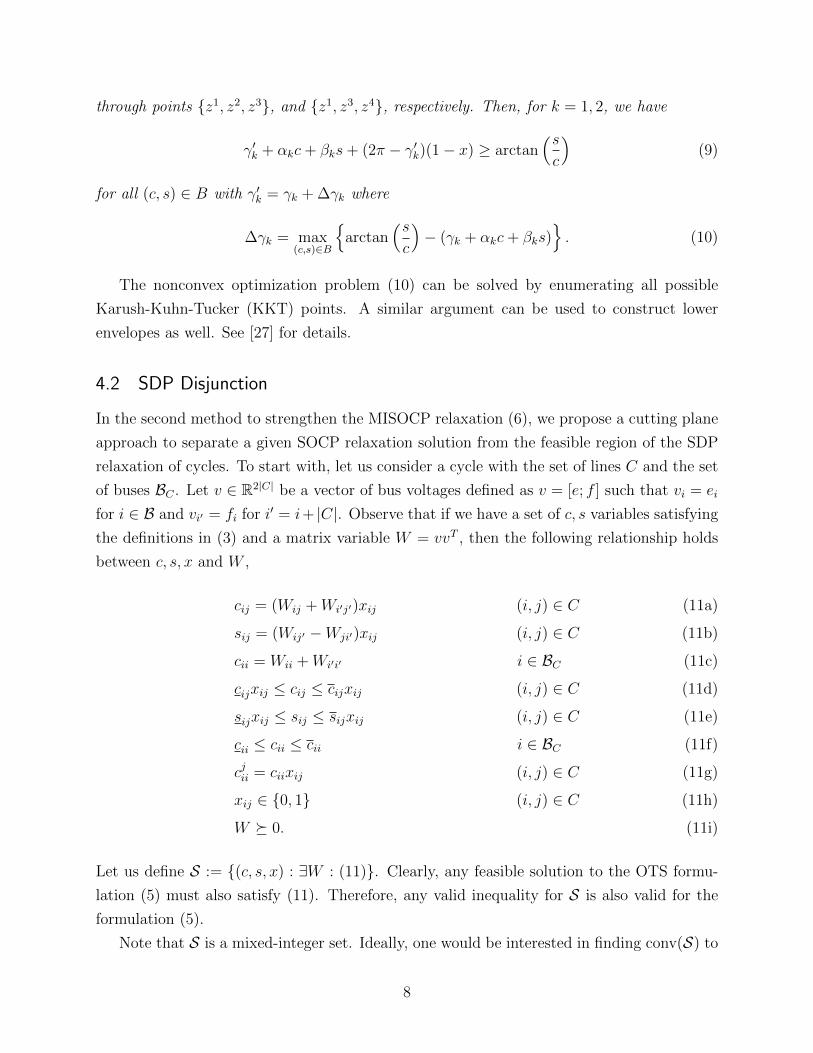
through points {z1, z2, z3}, and {z1, z3, z4}, respectively. Then, for k = 1, 2, we have

γ′k + αkc+ βks+ (2π − γ′k)(1− x) ≥ arctan(sc

)(9)

for all (c, s) ∈ B with γ′k = γk + ∆γk where

∆γk = max(c,s)∈B

{arctan

(sc

)− (γk + αkc+ βks)

}. (10)

The nonconvex optimization problem (10) can be solved by enumerating all possible

Karush-Kuhn-Tucker (KKT) points. A similar argument can be used to construct lower

envelopes as well. See [27] for details.

4.2 SDP Disjunction

In the second method to strengthen the MISOCP relaxation (6), we propose a cutting plane

approach to separate a given SOCP relaxation solution from the feasible region of the SDP

relaxation of cycles. To start with, let us consider a cycle with the set of lines C and the set

of buses BC . Let v ∈ R2|C| be a vector of bus voltages defined as v = [e; f ] such that vi = ei

for i ∈ B and vi′ = fi for i′ = i+ |C|. Observe that if we have a set of c, s variables satisfying

the definitions in (3) and a matrix variable W = vvT , then the following relationship holds

between c, s, x and W ,

cij = (Wij +Wi′j′)xij (i, j) ∈ C (11a)

sij = (Wij′ −Wji′)xij (i, j) ∈ C (11b)

cii = Wii +Wi′i′ i ∈ BC (11c)

cijxij ≤ cij ≤ cijxij (i, j) ∈ C (11d)

sijxij ≤ sij ≤ sijxij (i, j) ∈ C (11e)

cii ≤ cii ≤ cii i ∈ BC (11f)

cjii = ciixij (i, j) ∈ C (11g)

xij ∈ {0, 1} (i, j) ∈ C (11h)

W � 0. (11i)

Let us define S := {(c, s, x) : ∃W : (11)}. Clearly, any feasible solution to the OTS formu-

lation (5) must also satisfy (11). Therefore, any valid inequality for S is also valid for the

formulation (5).

Note that S is a mixed-integer set. Ideally, one would be interested in finding conv(S) to

8

generate strong valid inequalities. However, this is a quite computationally challenging task,

no easier than solving the original MINLP. Instead, we outer-approximate conv(S) and obtain

cutting planes by utilizing a simple disjunction for a cycle C: Either every line is active,

that is∑

(i,j)∈C xij = |C|, or at least one line is disconnected, that is∑

(i,j)∈C xij ≤ |C| − 1.

Below, we approximate these two disjunctions.

Disjunction 1: In the first disjunction, we have xij = 1 for all (i, j) ∈ C. Let us consider

the following constraints

cij = Wij +Wi′j′ (i, j) ∈ C (12a)

sij = Wij′ −Wji′ (i, j) ∈ C (12b)

cii = cjii (i, j) ∈ C (12c)

xij = 1 (i, j) ∈ C, (12d)

and define S1 := {(c, s, x) : ∃W : (12), (11c)− (11f), (11i)}.Disjunction 0: In the second disjunction, xij = 0 for some (i, j) ∈ C. Let us consider the

following constraints

c2ij + s2ij ≤ cjiicijj (i, j) ∈ C (13a)

ciixij ≤ cjii ≤ ciixij (i, j) ∈ C (13b)

cii − cii(1− xij) ≤ cjii (i, j) ∈ C (13c)

cjii ≤ cii − cii(1− xij) (i, j) ∈ C (13d)

0 ≤ xij ≤ 1 (i, j) ∈ C (13e)∑(i,j)∈C

xij ≤ |C| − 1, (13f)

and define S0 := {(c, s, x) : (13), (11d)-(11f)}.We note that both S1 and S0 are conic representable. In particular, these bounded sets

are respectively semidefinite and second-order cone representable. Therefore, conv(S1 ∪ S0)is also conic representable (see Appendix A on how to obtain a representation as an extended

formulation), and by construction, contains S.

Now, suppose a point (c∗, s∗, x∗) is given. We want to decide whether this point belongs

to conv(S1∪S0) or otherwise, find a separating hyperplane. Given that we have an extended

semidefinite representation for conv(S1 ∪ S0), we can solve an SDP separation problem to

achieve this. See Appendix B.

9

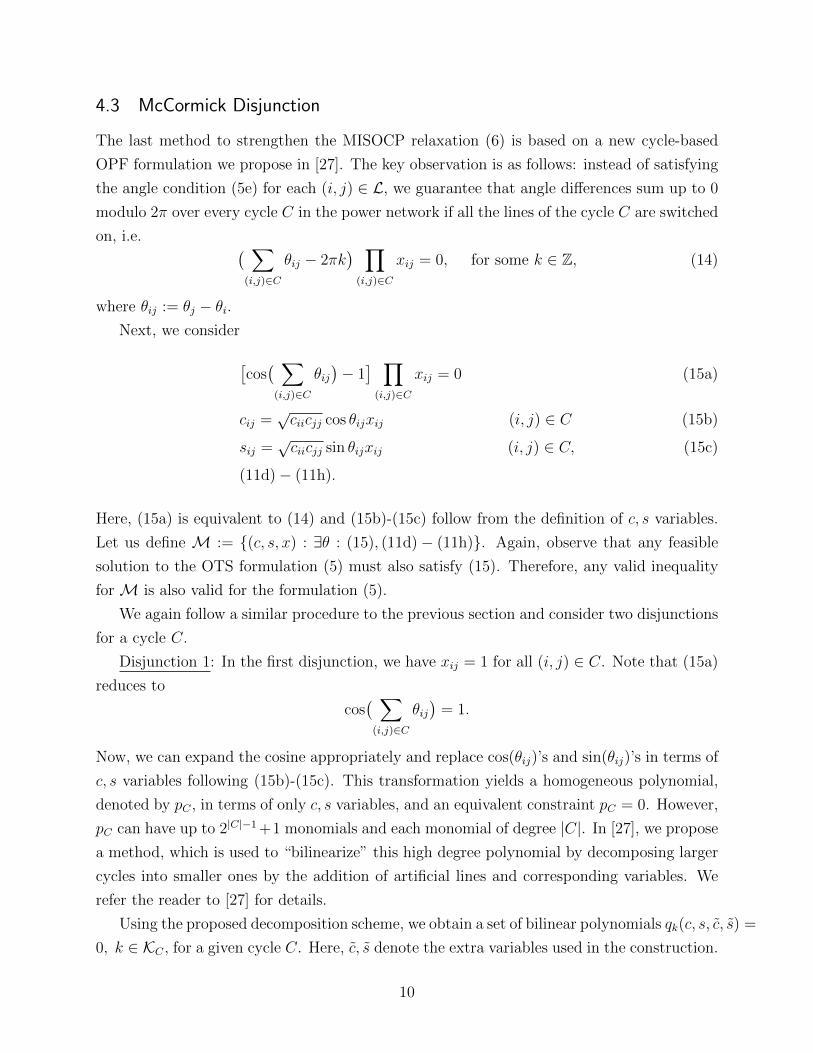
4.3 McCormick Disjunction

The last method to strengthen the MISOCP relaxation (6) is based on a new cycle-based

OPF formulation we propose in [27]. The key observation is as follows: instead of satisfying

the angle condition (5e) for each (i, j) ∈ L, we guarantee that angle differences sum up to 0

modulo 2π over every cycle C in the power network if all the lines of the cycle C are switched

on, i.e. ( ∑(i,j)∈C

θij − 2πk) ∏(i,j)∈C

xij = 0, for some k ∈ Z, (14)

where θij := θj − θi.Next, we consider

[cos( ∑(i,j)∈C

θij)− 1] ∏(i,j)∈C

xij = 0 (15a)

cij =√ciicjj cos θijxij (i, j) ∈ C (15b)

sij =√ciicjj sin θijxij (i, j) ∈ C, (15c)

(11d)− (11h).

Here, (15a) is equivalent to (14) and (15b)-(15c) follow from the definition of c, s variables.

Let us define M := {(c, s, x) : ∃θ : (15), (11d)− (11h)}. Again, observe that any feasible

solution to the OTS formulation (5) must also satisfy (15). Therefore, any valid inequality

for M is also valid for the formulation (5).

We again follow a similar procedure to the previous section and consider two disjunctions

for a cycle C.

Disjunction 1: In the first disjunction, we have xij = 1 for all (i, j) ∈ C. Note that (15a)

reduces to

cos( ∑(i,j)∈C

θij)

= 1.

Now, we can expand the cosine appropriately and replace cos(θij)’s and sin(θij)’s in terms of

c, s variables following (15b)-(15c). This transformation yields a homogeneous polynomial,

denoted by pC , in terms of only c, s variables, and an equivalent constraint pC = 0. However,

pC can have up to 2|C|−1+1 monomials and each monomial of degree |C|. In [27], we propose

a method, which is used to “bilinearize” this high degree polynomial by decomposing larger

cycles into smaller ones by the addition of artificial lines and corresponding variables. We

refer the reader to [27] for details.

Using the proposed decomposition scheme, we obtain a set of bilinear polynomials qk(c, s, c, s) =

0, k ∈ KC , for a given cycle C. Here, c, s denote the extra variables used in the construction.

10

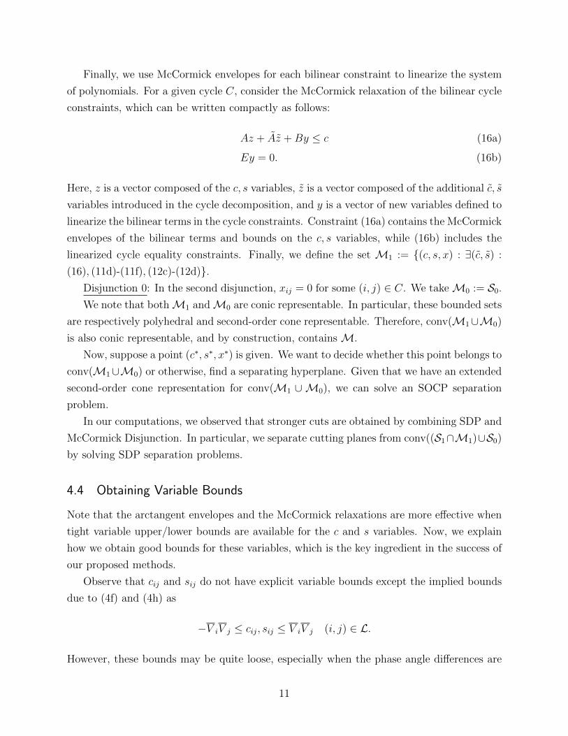
Finally, we use McCormick envelopes for each bilinear constraint to linearize the system

of polynomials. For a given cycle C, consider the McCormick relaxation of the bilinear cycle

constraints, which can be written compactly as follows:

Az + Az +By ≤ c (16a)

Ey = 0. (16b)

Here, z is a vector composed of the c, s variables, z is a vector composed of the additional c, s

variables introduced in the cycle decomposition, and y is a vector of new variables defined to

linearize the bilinear terms in the cycle constraints. Constraint (16a) contains the McCormick

envelopes of the bilinear terms and bounds on the c, s variables, while (16b) includes the

linearized cycle equality constraints. Finally, we define the set M1 := {(c, s, x) : ∃(c, s) :

(16), (11d)-(11f), (12c)-(12d)}.Disjunction 0: In the second disjunction, xij = 0 for some (i, j) ∈ C. We takeM0 := S0.We note that bothM1 andM0 are conic representable. In particular, these bounded sets

are respectively polyhedral and second-order cone representable. Therefore, conv(M1∪M0)

is also conic representable, and by construction, contains M.

Now, suppose a point (c∗, s∗, x∗) is given. We want to decide whether this point belongs to

conv(M1∪M0) or otherwise, find a separating hyperplane. Given that we have an extended

second-order cone representation for conv(M1 ∪ M0), we can solve an SOCP separation

problem.

In our computations, we observed that stronger cuts are obtained by combining SDP and

McCormick Disjunction. In particular, we separate cutting planes from conv((S1∩M1)∪S0)by solving SDP separation problems.

4.4 Obtaining Variable Bounds

Note that the arctangent envelopes and the McCormick relaxations are more effective when

tight variable upper/lower bounds are available for the c and s variables. Now, we explain

how we obtain good bounds for these variables, which is the key ingredient in the success of

our proposed methods.

Observe that cij and sij do not have explicit variable bounds except the implied bounds

due to (4f) and (4h) as

−V iV j ≤ cij, sij ≤ V iV j (i, j) ∈ L.

However, these bounds may be quite loose, especially when the phase angle differences are

11

small, implying cij ≈ 1 and sij ≈ 0 when the corresponding line is switched on. Therefore,

one should try to improve these bounds.

We adapt the procedure proposed in [27] (which dealt only with OPF) to the case of OTS

in order to obtain variable bounds, that is, we solve a reduced version of the full MISOCP

relaxation to efficiently compute bounds. In particular, to find variable bounds for ckl and

skl for some (k, l) ∈ L, consider the buses which can be reached from either k or l in at most

r steps. Denote this set of buses as Bkl(r). For instance, Bkl(0) = {k, l}, Bkl(1) = δ(k)∪δ(l),etc. We also define Gkl(r) = Bkl(r) ∩ G and Lkl(r) = {(i, j) ∈ L : i ∈ Bkl(r) or j ∈ Bkl(r)}.Then, we consider the following SOCP relaxation:

pgi − pdi = giicii +∑j∈δ(i)

pij i ∈ Bkl(r) (17a)

qgi − qdi = −biicii +∑j∈δ(i)

qij i ∈ Bkl(r) (17b)

pij = −Gijcjii +Gijcij −Bijsij (i, j) ∈ Lkl(r) (17c)

qij = Bijcjii −Bijcij −Gijsij (i, j) ∈ Lkl(r) (17d)

p2ij + q2ij ≤ (Smaxij )2 (i, j) ∈ Lkl(r) (17e)

V 2i ≤ cii ≤ V

2

i i ∈ Bkl(r + 1) (17f)

pmini ≤ pgi ≤ pmax

i i ∈ Gkl(r) (17g)

qmini ≤ qgi ≤ qmax

i i ∈ Gkl(r) (17h)

cijxij ≤ cij ≤ cijxij (i, j) ∈ Lkl(r) (17i)

sijxij ≤ sij ≤ sijxij (i, j) ∈ Lkl(r) (17j)

ciixij ≤ cjii ≤ ciixij (i, j) ∈ Lkl(r) (17k)

cii − cii(1− xij) ≤ cjii (i, j) ∈ Lkl(r) (17l)

cjii ≤ cii − cii(1− xij) (i, j) ∈ Lkl(r) (17m)

cij = cji, sij = −sji (i, j) ∈ Lkl(r) (17n)

c2ij + s2ij ≤ cjiicijj (i, j) ∈ Lkl(r) (17o)

0 ≤ xij ≤ 1 (i, j) ∈ Lkl(r) (17p)

xkl = 1. (17q)

Essentially, (17) is the continuous relaxation of MISOCP relaxation applied to the part of

the power network within r steps of the buses k and l. ckl and skl can be minimized and

maximized subject to (17) for each edge (k, l) to obtain lower and upper bounds, respectively.

These SOCPs can be solved in parallel, since they are independent of each other. It is

12

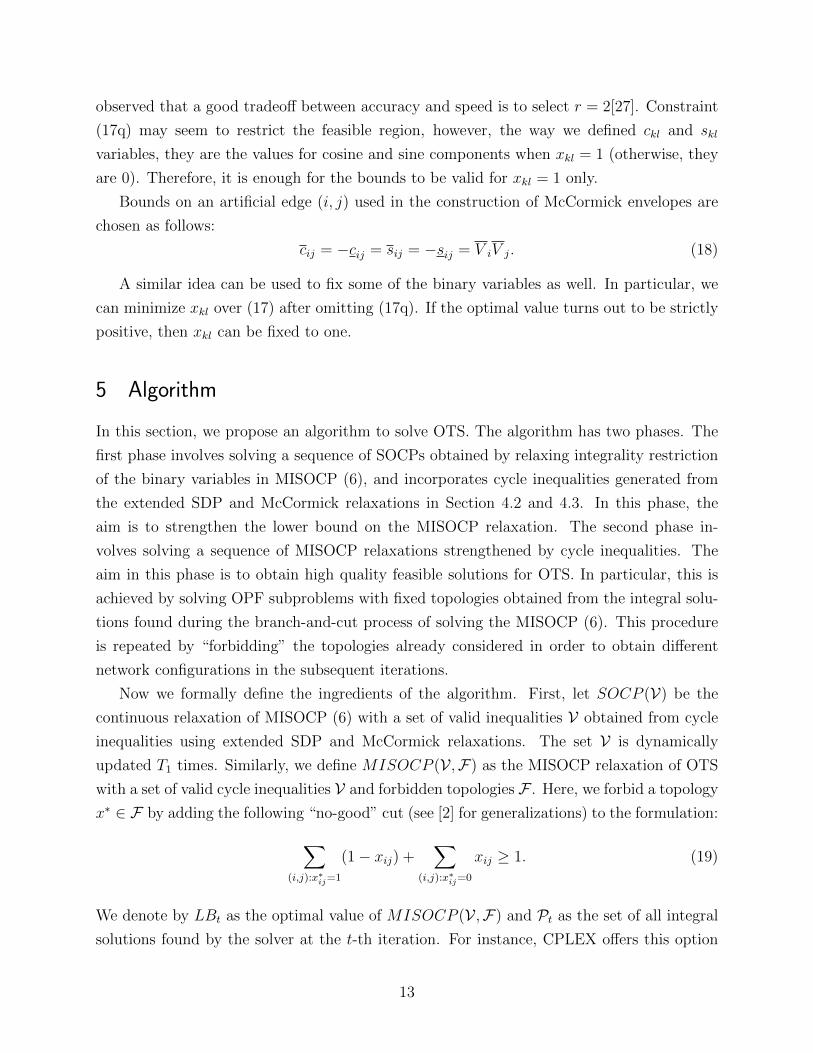
observed that a good tradeoff between accuracy and speed is to select r = 2[27]. Constraint

(17q) may seem to restrict the feasible region, however, the way we defined ckl and skl

variables, they are the values for cosine and sine components when xkl = 1 (otherwise, they

are 0). Therefore, it is enough for the bounds to be valid for xkl = 1 only.

Bounds on an artificial edge (i, j) used in the construction of McCormick envelopes are

chosen as follows:

cij = −cij = sij = −sij = V iV j. (18)

A similar idea can be used to fix some of the binary variables as well. In particular, we

can minimize xkl over (17) after omitting (17q). If the optimal value turns out to be strictly

positive, then xkl can be fixed to one.

5 Algorithm

In this section, we propose an algorithm to solve OTS. The algorithm has two phases. The

first phase involves solving a sequence of SOCPs obtained by relaxing integrality restriction

of the binary variables in MISOCP (6), and incorporates cycle inequalities generated from

the extended SDP and McCormick relaxations in Section 4.2 and 4.3. In this phase, the

aim is to strengthen the lower bound on the MISOCP relaxation. The second phase in-

volves solving a sequence of MISOCP relaxations strengthened by cycle inequalities. The

aim in this phase is to obtain high quality feasible solutions for OTS. In particular, this is

achieved by solving OPF subproblems with fixed topologies obtained from the integral solu-

tions found during the branch-and-cut process of solving the MISOCP (6). This procedure

is repeated by “forbidding” the topologies already considered in order to obtain different

network configurations in the subsequent iterations.

Now we formally define the ingredients of the algorithm. First, let SOCP (V) be the

continuous relaxation of MISOCP (6) with a set of valid inequalities V obtained from cycle

inequalities using extended SDP and McCormick relaxations. The set V is dynamically

updated T1 times. Similarly, we define MISOCP (V ,F) as the MISOCP relaxation of OTS

with a set of valid cycle inequalities V and forbidden topologies F . Here, we forbid a topology

x∗ ∈ F by adding the following “no-good” cut (see [2] for generalizations) to the formulation:∑(i,j):x∗ij=1

(1− xij) +∑

(i,j):x∗ij=0

xij ≥ 1. (19)

We denote by LBt as the optimal value of MISOCP (V ,F) and Pt as the set of all integral

solutions found by the solver at the t-th iteration. For instance, CPLEX offers this option

13

called solution pool. In a practical implementation, this part is repeated T2 times.

Let OPF (x) denote the value of a feasible solution to OPF problem (4) for the fixed

topology induced by the integral vector x. Finally, UB is the best upper bound on OTS.

Now, we present Algorithm 1.

Algorithm 1 OTS algorithm.

Input: T1, T2, ε.Phase I: Set V ← ∅, F ← ∅, UB ←∞.for τ = 1, . . . , T1 do

Solve SOCP (V).Separate cycle inequalities for each cycle in a cycle basis to obtain a set of valid inequal-ities Vτ .Update V ← V ∪ Vτ .

end forPhase II: Set t← 0.repeatt← t+ 1Solve MISOCP (V ,F) to obtain a pool of integral solutions Pt and record the optimalcost as LBt.for all x ∈ Pt doif OPF (x) < UB thenUB ← OPF (x)

end ifend forUpdate F ← F ∪ Pt.

until LBt ≥ (1− ε)UB or t ≥ T2

Observation 5.1. If OPF (x) returns globally optimal solution for every topology x, ε = 0

and T2 = ∞, then Algorithm 1 converges to the optimal solution of OTS in finitely many

iterations.

Observation 5.1 follows from the fact that there are finitely many topologies and by the

hypothesis that OPF (x) can be solved globally, which is possible for some IEEE instances

using moment/sum-of-squares relaxations [24]. Although Observation 5.1 states that Al-

gorithm 1 can be used to solve OTS to global optimality in finitely many iterations, the

requirement of solving OPF (x) to global optimality may not be satisfied always. In prac-

tice, we can solve OPF subproblems using local solver, in which case we have Observation

5.2.

Observation 5.2. If OPF (x) is solved by a local solution method, then we have LB1 ≤z∗ ≤ UB upon termination of Algorithm 1, where z∗ is the optimal value of OTS.

14

6 Computational Experiments

In this section, we present the results of our extensive computational experiments on standard

IEEE instances available from MATPOWER [48] and instances from NESTA 0.3.0 archive

with congested operating conditions [7]. The code is written in the C# language with Visual

Studio 2010 as the compiler. For all experiments, we used a 64-bit computer with Intel Core

i5 CPU 2.50GHz processor and 16 GB RAM. Time is measured in seconds. We use three

different solvers:

• CPLEX 12.6 [1] to solve MISOCPs.

• Conic interior point solver MOSEK 7.1 [37] to solve SDP separation problems.

• Nonlinear interior point solver IPOPT [46] to find local optimal solutions to OPF (x).

We use a Gaussian elimination based approach to construct a cycle basis proposed in [29]

and use this set of cycles in the separation phase.

6.1 Methods

We report the results of three algorithmic settings:

• SOCP: MISOCP formulation (6) in Phase II without Phase I (i.e. T1 = 0).

• SOCPA: SOCP strengthened by the arctangent envelopes introduced in Section 4.1.

• SOCPA Disj: SOCPA strengthened further by dynamically generating linear valid in-

equalities obtained from separating an SOCP feasible solution from the SDP and Mc-

Cormick relaxation over cycles using a disjunctive argument T1 times. In particular, a

separation oracle is used to separate a given point from conv((S1 ∩M1) ∪ S0).

The following four performance measures are used to assess the accuracy and the efficiency

of the proposed methods:

• “%OG” is the percentage optimality gap proven by our algorithm calculated as 100×(1 − LB1/UB). Here, LB1 is the lower bound proven, which may be strictly smaller

than LB1 due to optimality gap tolerance and time limit.

• “%CB” is the percentage cost benefit obtained by line switching calculated as 100 ×(1 − UB/OPF (e)), where e is the vector of ones so that OPF (e) corresponds to the

OPF solution with the initial topology.

15

• “#off” is the number of lines switched off in the topology which gives UB.

• “TT” is the total time in seconds, including preprocessing (bound tightening), solution

of T1 = 5 rounds of SOCPs to improve lower bound and separation problems to generate

cutting planes (in the case of SOCPA Disj), solution of T2 rounds of MISOCPs and

several calls to local solver IPOPT with given topologies. MISOCPs are solved under

720 seconds time limit so that 5 iterations take about 1 hour (optimality gap for integer

programs is 0.01%). Preprocessing and separation subproblems are parallelized.

We choose parameter T2 = 5 and pre-terminate Algorithm 1 if 0.1% optimality gap is proven.

6.2 Results

The results of our computational experiments are presented in Tables 1 and 2 for standard

IEEE and NESTA instances, respectively. We considered instances up to 300-bus since

Phase II of the Algorithm 1 does not scale up well for larger instances. Let us start with the

former: IEEE instances are a relatively easy set since transmission line limits are generally

not binding. Therefore, cost benefits obtained by switching are also limited. The largest

cost reduction is obtained for case30Q with 2.24%. Among the three methods, the most

successful one is SOCPA Disj, on average proving 0.05% optimality gap and providing 0.31%

cost savings. In terms of computational time, SOCP is the fastest, however, its performance

is not as good as the other two. Quite interestingly, SOCPA Disj is faster than SOCPA, on

average, for this set of instances. In terms of comparison with other methods, unfortunately,

there is limited literature for this purpose. In [18], nine of these instances (except for cases

9Q and 30Q) are considered and a quadratic convex (QC) relaxation based approach is

used. On average, their approach proves 0.14% optimality gap, which is worse than any

of our methods over the same nine instances. The only instance QC approach is better is

118ieee with 0.11% optimality gap, while it is worse than our methods for case300 with a

0.47% optimality gap.

16

Table 1: Results summary for standard IEEE Instances.

SOCP SOCPA SOCPA Disj

case %OG %CB #off TT(s) %OG %CB #off TT(s) %OG %CB #off TT(s)

6ww 0.16 0.48 2 1.29 0.02 0.48 2 0.67 0.01 0.48 2 1.28

9 0.00 0.00 0 0.26 0.00 0.00 0 0.22 0.00 0.00 0 0.55

9Q 0.04 0.00 0 0.42 0.04 0.00 0 0.33 0.04 0.00 0 0.97

14 0.08 0.00 0 0.66 0.09 0.00 0 0.70 0.01 0.00 1 1.81

ieee30 0.05 0.00 1 1.95 0.05 0.00 0 1.67 0.02 0.00 1 3.84

30 0.07 0.52 1 4.60 0.06 0.52 2 5.01 0.03 0.51 2 9.39

30Q 0.44 2.05 2 24.43 0.43 2.03 5 25.80 0.13 2.24 5 44.16

39 0.03 0.00 0 2.53 0.01 0.02 1 3.17 0.01 0.02 1 4.48

57 0.07 0.02 4 6.18 0.07 0.02 4 8.72 0.08 0.01 1 13.59

118 0.19 0.08 4 3065.64 0.15 0.12 10 2553.59 0.17 0.08 16 3174.01

300 0.16 0.02 9 2318.89 0.15 0.03 12 3624.12 0.10 0.05 15 2803.31

Avg. 0.12 0.29 2.1 493.35 0.10 0.29 3.3 565.82 0.05 0.31 4.0 550.67

Table 2: Results summary for NESTA Instances from Congested Operating Conditions.

SOCP SOCPA SOCPA Disj

case %OG %CB #off TT(s) %OG %CB #off TT(s) %OG %CB #off TT(s)

3lmbd 3.30 0.00 0 0.14 2.00 0.00 0 0.14 1.17 0.00 0 0.30

4gs 0.65 0.00 0 0.11 0.16 0.00 0 0.13 0.00 0.00 0 0.27

5pjm 0.18 0.27 1 0.61 0.01 0.27 1 0.41 0.02 0.27 1 0.89

6ww 6.06 7.74 1 1.23 1.34 7.74 1 1.64 1.05 7.74 1 1.97

9wscc 0.00 0.00 0 0.19 0.00 0.00 0 0.20 0.00 0.00 0 0.30

14ieee 1.02 0.33 1 2.86 0.89 0.45 2 3.48 0.41 0.45 2 4.49

29edin 0.43 0.00 2 12.79 0.24 0.18 13 299.82 0.33 0.08 21 181.74

30as 1.81 3.13 2 14.82 0.35 3.30 5 19.52 0.34 3.30 5 24.93

30fsr 3.24 44.20 2 9.72 0.05 44.98 2 4.76 0.03 44.98 3 6.97

30ieee 0.54 0.46 1 12.28 0.40 0.48 2 10.61 0.15 0.48 2 13.37

39epri 1.92 1.10 1 11.56 0.80 1.41 2 13.20 0.70 1.52 2 12.65

57ieee 0.12 0.10 3 41.48 0.12 0.10 2 58.97 0.09 0.10 3 29.86

118ieee 41.67 4.33 3 225.57 21.51 27.98 30 3838.62 7.50 39.09 21 3856.76

162ieee 0.57 1.05 9 3675.75 0.63 1.00 15 3861.29 0.60 1.00 15 3855.50

189edin 5.31 1.10 3 540.02 4.81 0.13 2 2194.80 5.58 0.00 0 3634.02

300ieee 1.00 0.10 12 3655.10 0.65 0.37 21 3640.14 0.61 0.35 21 3651.95

Avg. 4.24 3.99 2.6 512.76 2.12 5.52 6.1 871.73 1.16 6.21 6.1 954.75

Now let us consider NESTA instances with congested operating conditions. This set is

particularly suited for line switching as more stringent transmission line limits are imposed.

17

In fact, large cost improvements are observed for some test cases. For instance, about

45% and 39% cost reductions are possible for cases 30fsr and 118ieee, respectively. Other

instances with sizable cost reductions include cases 6ww and 30as. SOCPA Disj is again the

most successful method if we look at averages of optimality gap (1.16%) and cost savings

(6.21%). It certifies that the best topology is within 1.17% of the optimal for all the cases

except for 118ieee and 189edin. In terms of computational time, SOCP is again the fastest,

however, its performance is significantly worse than the other two. We also note that SOCPA

improves quite a bit over SOCP in terms of optimality and cost benefits with 70% increase

in computational time. SOCPA Disj takes about only 10% more time than SOCPA. As we go

from SOCP to SOCPA Disj, problems get more complicated and sometimes, MISOCPs are

not solved to optimality within time limit. Consequently, for cases 189edin and 300ieee, the

optimality gaps proven and cost benefits obtained by SOCPA Disj can be slightly worse.

Finally, we note that that optimality gaps can be explained by two non-convexities: 1)

integrality, 2) power flow equations. For instance, in case 3lmbd, the optimality gap can only

be explained by the non-convexity of power flow equation since all the relevant topologies

are considered. Similarly, at least some portion of the relatively large optimality gaps for

cases 118ieee and 189edin may be attributed to non-convexity of power flow equations.

Consequently, any future improvements on strengthening the convex relaxations of OPF

problem can be useful in closing more gaps in OTS as well.

6.3 Discussion

In this section, we take a closer look at some of the instances with large cost benefits

and try to gain some insight as to 1) how these large savings are obtained, and 2) how

simple heuristics may fail to produce comparable results. Firstly, using a small example, we

illustrate how large cost savings can be obtained. Secondly, we compare the results of our

algorithm with a commonly used heuristic based on switching the best line and demonstrate

how different the solution quality can be.

To address the first issue, let us concentrate on a small instance, namely case6ww from

NESTA archive. This instance has the same topology and line characteristics as the standard

IEEE test case but load and generation parameters are slightly different. In particular,

pdi = 78.24, qdi = 70, V i = 0.95 and V i = 1.05 for the load buses i = 4, 5, 6 while the data for

generation buses 1, 2 and 3 is summarized in Table 3. With this topology, the local optimal

solution obtained using IPOPT with objective value of 273.76 is given in Figure 1. We note

that the lines (1, 5), (2, 4) and (3, 6) are congested in this configuration. On the other hand,

if the line (1, 2) is switched off, then the objective value reduces to 252.57, corresponding to a

18

Table 3: Generator data for NESTA case6ww test case.

pmini pmax

i qmini qmax

i V i = V i cost1 25 200 −100 100 1.05 1.2763112 18.75 106 −100 100 1.05 0.5862723 22.5 93 −100 100 1.07 1.29111

7.74% cost saving over the initial topology. The difference is due to the fact that the outputs

of generators 1 and 2 are now changed to (85.56, 32.74) and (84.25, 63.26), respectively.

Notice that with the new topology, the cheaper generator 2 is used more, which results in

the cost reduction. In the initial topology, this is not possible since the voltage magnitudes

of the generators are fixed, and lines (1, 5) and (2, 4) are congested.

Figure 1: Flow diagram for the solution of NESTA case6ww without any line switching.The numbers above each generator node respectively represent the active and reactive poweroutput. Similarly, the numbers near each edge respectively represent the active and reactivepower flow of the line in the direction from the small indexed bus to the large indexed one.The figure is generated by modifying [33].

Bus 1

Bus 2

Bus 3

Bus 4

Bus 5

Bus 6

(29.88,−15.92) (1.14,−11.93)

(4.15,−4.85) (0.91,−9.82)

(47.36, 20.85) (17.30, 15.89) (51.32, 61.37)

(38.19, 11.88) (22.5

7,22.93

)

(37.9

6,46.46

) (27.85, 12.84)

(115.44, 16.81)

(55.35, 76.74)

(72.79, 89.66)

(78.24, 70)

(78.24, 70)

(78.24, 70)

Now, let us consider the second issue. Due to the combinatorial nature of OTS problem,

heuristics are frequently used to obtain suboptimal solutions. A commonly used one is to

switch off a single line to obtain cost benefits [41, 31]. Although this heuristic idea is easy

19

to implement and works well in some instances, there are no guarantees on its accuracy. For

example, in case6ww, the best line to switch off is, in fact, (1, 2) suggested by both the best

line heuristic and our algorithm. However, for other problems with large cost benefits, this is

not always the case. For instance, in case30as and case30fsr, the best line heuristic reduces

the overall cost to 2.99% and 44.02% respectively, compared to 3.30% and 44.98% obtained

from our algorithm. For case118ieee, the cost reduction is dramatically different. The

best line heuristic reduces the cost only by 19.52% while our algorithm provides a topology

with 39.09% saving. Moreover, the best line heuristic does not provide any guarantee on

how good the solution is while our algorithm gives optimality guarantees by construction.

Therefore, adapting Algorithm 1 in real-time operations can yield significant savings over

simple heuristics.

7 Conclusions

In this paper, we proposed a systematic approach to solve the AC OTS problem. In particu-

lar, we presented an alternative formulation for OTS and constructed a MISOCP relaxation.

We improved the strength of this relaxation by the addition of arctangent envelopes and

cutting planes obtained using disjunctive techniques. The use of these disjunctive cuts help

in closing gap significantly. Our experiments on standard and congested instances suggest

that the proposed methods are effective in obtaining strong lower bounds and producing

provably good feasible solutions.

We remind the reader that AC OTS is a challenging problem since it embodies two types

of non-convexities due to AC power flow constraints and integrality of variables. We hope

that the methodology developed in this paper can eventually be further improved to solve

AC OTS problem in real life operations. As a future work, we would like to pursue finding

ways to improve the solution time of MISOCPs as this step is the bottleneck in Algorithm

1. Also, decomposition methods can be sought to solve large-scale problems more efficiently,

which could make the proposed approach adaptable to real life instances.

A Convex Hull of Union of Two Conic Representable Sets

Let S1 and S2 be two bounded, conic representable sets

Si = {x : ∃ui : Aix+Biui �Ki

bi} i = 1, 2.

20

Here, Ki’s are regular (closed, convex, pointed with non-empty interior) cones. Then, a conic

representation for conv(S1 ∪ S2) is given as follows:

x = x1 + x2, λ1 + λ2 = 1, λ1, λ2 ≥ 0

Aixi +Biu

i �Kibiλi i = 1, 2.

B Separation from an Extended Conic Representable Set

Let S be a conic representable set S = {x : ∃u : Ax+Bu �K b}. Here, K is a regular cone.

Suppose we want to decide if a given point x∗ belongs to S and find a separating hyperplane

α>x ≥ β if x∗ /∈ S. This problem can be formulated as maxα,β{β − α>x∗ : α>x ≥ β ∀x ∈ S

},

where the constraint can be further dualized as

Z∗ := maxα,β,µ{β − α>x∗ : b>µ ≥ β,A>µ = α,B>µ = 0,

µ ∈ K∗,−e ≤ α ≤ e,−1 ≤ β ≤ 1},

where K∗ is the dual cone of K. If Z∗ ≤ 0, then x∗ ∈ S, otherwise, the optimal α, β from

the above program gives the desired separating hyperplane. For details, please see [27].

References

[1] User’s Manual for CPLEX Version 12.6. IBM, 2014.

[2] Gustavo Angulo, Shabbir Ahmed, Santanu S Dey, and Volker Kaibel. Forbidden vertices.

Mathematics of Operations Research, 40(2):350–360, 2014.

[3] X. Bai, H. Wei, K. Fujisawa, and Y. Wang. Semidefinite programming for optimal

powerflow problems. International Journal on Electric Power Energy Systems, 30(6-

7):383–392, 2008.

[4] C. Barrows, S. Blumsack, and R. Bent. Computationally efficient optimal transmission

switching: Solution space reduction. In Power and Energy Society General Meeting,

2012 IEEE, pages 1–8, July 2012.

[5] C. Barrows, S. Blumsack, and P. Hines. Correcting optimal transmission switching for

AC power flows. In 47th Hawaii International Conference on System Sciences (HICSS),

page 2374–2379, 2014.

21

[6] D. Bienstock and G. Munoz. On linear relaxations of OPF problems. arXiv preprint

arXiv:1411.1120, 2014.

[7] C. Coffrin, D. Gordon, and P. Scott. NESTA, The NICTA energy system test case

archive. arXiv preprint arXiv:1411.0359, 2014.

[8] C. Coffrin, H. L. Hijazi, and P. Van Hentenryck. The QC relaxation: Theoretical and

computational results on optimal power flow. arXiv preprint arXiv:1502.07847, 2015.

[9] C. Coffrin and P. Van Hentenryck. A linear-programming approximation of AC power

flows. INFORMS Journal on Computing, 26(4):718–734, 2014.

[10] A. G. Exposito and E. R. Ramos. Reliable load flow technique for radial distribution

networks. IEEE Trans. on Power Syst., 14(3):1063 – 1069, 1999.

[11] R.S. Ferreira, C.L.T. Borges, and M.V.F. Pereira. A flexible mixed-integer linear pro-

gramming approach to the AC optimal power flow in distribution systems. IEEE Trans.

on Power Syst., 29(5):2447–2459, Sept 2014.

[12] E.B. Fisher, R.P. O’Neill, and M.C. Ferris. Optimal transmission switching. IEEE

Trans. on Power Syst., pages 1346–1355, 2008.

[13] J.D. Fuller, R. Ramasra, and A. Cha. Fast heuristics for transmission-line switching.

IEEE Trans. on Power Syst., 27(3):1377–1386, Aug 2012.

[14] J. Han and A. Papavasiliou. The impacts of transmission topology control on the

European electricity network. IEEE Trans. on Power Syst., 31(1):496–507, Jan 2016.

[15] K.W. Hedman, M.C. Ferris, R.P. O’Neill, E.B. Fisher, and S.S. Oren. Co-optimization

of generation unit commitment and transmission switching with N-1 reliability. IEEE

Trans. on Power Syst., 25(2):1052–1063, May 2010.

[16] K.W. Hedman, R.P. O’Neill, E.B. Fisher, and S.S. Oren. Optimal transmission switching

with contingency analysis. IEEE Trans. on Power Syst., 24(3):1577–1586, Aug 2009.

[17] K.W. Hedman, S.S. Oren, and R.P. O’Neill. A review of transmission switching and

network topology optimization. In Power and Energy Society General Meeting, 2011

IEEE, pages 1–7, July 2011.

[18] HL Hijazi, C Coffrin, and P Van Hentenryck. Convex quadratic relaxations of mixed-

integer nonlinear programs in power systems. Technical report, NICTA, Canberra, ACT

Australia, 2013.

22

[19] R. A. Jabr. Radial distribution load flow using conic programming. IEEE Trans. on

Power Syst., 21(3):1458–1459, 2006.

[20] R. A. Jabr. A conic quadratic format for the load flow equations of meshed networks.

IEEE Trans. on Power Syst., 22(4):2285–2286, 2007.

[21] R. A. Jabr. Optimal power flow using an extended conic quadratic formulation. IEEE

Trans. on Power Syst., 23(3):1000–1008, 2008.

[22] R.A. Jabr. Optimization of AC transmission system planning. IEEE Trans. on Power

Syst., 28(3):2779–2787, Aug 2013.

[23] R.A. Jabr, R. Singh, and B.C. Pal. Minimum loss network reconfiguration using mixed-

integer convex programming. IEEE Trans. on Power Syst., 27(2):1106–1115, May 2012.

[24] Cedric Josz and Daniel K. Molzahn. Moment/sum-of-squares hierarchy for complex

polynomial optimization. arXiv:1508.02068, 2015.

[25] M. Khanabadi, H. Ghasemi, and M. Doostizadeh. Optimal transmission switching

considering voltage security and N-1 contingency analysis. IEEE Trans. on Power

Syst., 28(1):542–550, Feb 2013.

[26] A. Khodaei, M. Shahidehpour, and S. Kamalinia. Transmission switching in expansion

planning. IEEE Trans. on Power Syst., 25(3):1722–1733, Aug 2010.

[27] B. Kocuk, S. S. Dey, and X. A. Sun. Strong SOCP relaxations for the optimal power

flow problem. to appear in Operations Research, 2016.

[28] B. Kocuk, S.S. Dey, and X.A. Sun. Inexactness of sdp relaxation and valid inequalities

for optimal power flow. Power Systems, IEEE Transactions on, 31(1):642–651, Jan

2016.

[29] B. Kocuk, H. Jeon, S. S. Dey, J. Linderoth, J. Luedtke, and X. A. Sun. A cycle-based

formulation and valid inequalities for DC power transmission problems with switching.

to appear in Operations Research, 2016.

[30] A.S. Korad and K.W. Hedman. Robust corrective topology control for system reliability.

IEEE Trans. on Power Syst., 28(4):4042–4051, Nov 2013.

[31] A.S. Korad and K.W. Hedman. Enhancement of do-not-exceed limits with robust cor-

rective topology control. to appear in IEEE Trans. on Power Syst., 2015.

23

[32] J. Lavaei and S. H. Low. Zero duality gap in optimal power flow problem. IEEE Trans.

on Power Syst., 27(1):92–107, 2012.

[33] Richard Lincoln. Learning to trade power. https://github.com/rwl/thesis/blob/

master/tikz/case6ww.tex, 2010.

[34] G. P. McCormick. Computability of global solutions to factorable nonconvex programs:

Part I – convex underestimating problems. Math. Prog., 10(1):147–175, 1976.

[35] D. K. Molzahn, J. T. Holzer, B. C. Lesieutre, and C. L DeMarco. Implementation of a

large-scale optimal power flow solver based on semidefinite programming. IEEE Trans.

on Power Syst., 28(4):3987–3998, 2013.

[36] D.K. Molzahn and I.A. Hiskens. Sparsity-exploiting moment-based relaxations of the

optimal power flow problem. To appear in IEEE Trans. on Power Syst., 2015.

[37] MOSEK. MOSEK Modeling Manual. MOSEK ApS, 2013.

[38] R. O’ Neill, R. Baldick, U. Helman, M. Rothkopf, and J. Stewart. Dispatchable trans-

mission in RTO markets. IEEE Trans. on Power Syst., 20(1):171–179, 2005.

[39] P. Ruiz, J. M. Forster, A. Rudkevich, and M. C. Caramanis. On fast transmission

topology control heuristics. IEEE Power and Energy Society General Meeting, pages

1–8, 2011.

[40] P. Ruiz, J. M. Forster, A. Rudkevich, and M. C. Caramanis. Tractable transmission

topology control using sensitivity analysis. IEEE Trans. on Power Syst., 27(3):1550–

1559, 2012.

[41] M. Sahraei-Ardakani, A. Korad, K.W. Hedman, P. Lipka, and S. Oren. Performance of

AC and DC based transmission switching heuristics on a large-scale polish system. In

PES General Meeting — Conference Exposition, 2014 IEEE, pages 1–5, July 2014.

[42] M. Soroush and J.D. Fuller. Accuracies of optimal transmission switching heuristics

based on DCOPF and ACOPF. IEEE Trans. on Power Syst., 29(2):924–932, March

2014.

[43] C. Thompson, K. McIntyre, S. Nuthalapati, A. Garcia, and E.A. Villanueva. Real-time

contingency analysis methods to mitigate congestion in the ERCOT region. In Power

Energy Society General Meeting, 2009. PES ’09. IEEE, pages 1–7, July 2009.

24

[44] P.A. Trodden, W.A. Bukhsh, A. Grothey, and K.I.M. McKinnon. Optimization-based

islanding of power networks using piecewise linear AC power flow. IEEE Trans. on

Power Syst., 29(3):1212–1220, May 2014.

[45] T. Van Acker, D. Van Hertem, D. Bekaert, K. Karoui, and C. Merckx. Implementation

of bus bar switching and short circuit constraints in optimal power flow problems. In

PowerTech, 2015 IEEE Eindhoven, pages 1–6, June 2015.

[46] A. Wachter and L. T. Biegler. On the implementation of an interior-point filter line-

search algorithm for large-scale nonlinear programming. Math. Prog., 106(1):25–57,

2006.

[47] J. Wu and K.W. Cheung. On selection of transmission line candidates for optimal

transmission switching in large power networks. In Power and Energy Society General

Meeting (PES), 2013 IEEE, pages 1–5, July 2013.

[48] R.D. Zimmerman, C.E. Murillo-Sanchez, and R.J. Thomas. MATPOWER: Steady-state

operations, planning, and analysis tools for power systems research and education. IEEE

Trans. Power Syst., 26(1):12–19, Feb 2011.

25