new features added to the purdue farm financial …ageconsearch.umn.edu/bitstream/161490/2/382a...

New Features Added to the Purdue Farm Financial Analysis Spreadsheet

By Freddie L. Barnard, Elizabeth A. Yeager, and Alan Miller

IntroductionSeveral computer software programs are available to record information needed to prepare income tax returns and to conduct financial analysis on historical data for a farm or ranch business. However, the use of an accrual-adjusted income statement to conduct such an analysis rather than a cash basis income statement is greatly needed in the volatile commodity price environment that currently characterizes agriculture. A Financial Analysis Spreadsheet available from Purdue University was recently updated and enhanced, and is available at no charge. The changes and enhancements made to that spreadsheet will be discussed in the following paragraphs and are identified using the subheading, new.

Freddie L. Barnard is a Professor with Purdue University. Elizabeth A. Yeager is Assistant Professor with Purdue University. Alan Miller is Farm Business Management Specialist with Purdue University.

2013 JOURNAL OF THE ASFMRA

74

ABSTRACT

The Purdue Farm Financial Analysis Spreadsheet originally introduced in 1998 has been updated to include the additional financial measures recommended by the Farm Financial Standards Council; EBITDA (Earnings Before Interest, Taxes, Depreciation, and Amortization), working capital to gross revenue ratio, capital debt repayment capacity and replacement margin, and the replacement margin coverage ratio. Also, an additional worksheet was added that calculates break-even at the farm level using the traditional fixed and variable classification of costs, as well as a second breakeven amount that includes principal payments on term loans, loss carryover amounts and replacement amounts for capital, such as machinery and equipment.


75

SpreadsheetDetails of the original version of the spreadsheet were published previously (Barnard & Boehlje, 2003; Wilson et al., 2007), so only a condensed overview of the spreadsheet will be presented here. The updated spreadsheet is discussed in detail in Farm Business Management for the 21st Century: Measuring and Analyzing Farm Financial Performance (Miller et al., 2012). Guidelines provided by the Farm Financial Standards Council (Financial Guidelines, 2008) are used to prepare the financial statements and calculate financial measures. The financial measures for an individual farm can then be compared to either benchmarks or industry averages.

Four features of the spreadsheet enable the user to cost-effectively analyze the financial condition and performance of an individual farm or ranch business, while investing a minimum amount of time and effort. Those features can then be used to better assess repayment risk for a farm/ranch business. First, an accrual-adjusted income statement is needed to accurately determine farm/ranch profitability, calculate financial measures and assess repayment capacity. A cash basis income statement generally will not accurately measure net farm income. Second, the DuPont financial analysis system can be used to assess the impact of changes in revenue and operating expenses on farm profitability. Third, the sensitivity of repayment capacity measures to changes in revenue and operating expenses can be evaluated. Fourth, the impact on the break-even revenue for the business resulting from changes in the above measures can be assessed. Each of these features is discussed in the paragraphs that follow.

Accrual-adjusted Income StatementThe benefits of using financial data reported on an accrual-adjusted income statement for reporting farm profitability and conducting financial analysis have been previously studied. The magnitude of the difference between net farm income calculated using a cash basis income statement and net farm income calculated using an accrual-adjusted income statement was reported in a 2010 article using University of Illinois Farm Business and Farm Management (FBFM) data. The study found the median annual difference between cash net farm income reported on a Schedule F in a Form 1040, U.S. Individual Income Tax Return, and net farm income reported on an accrual-adjusted basis ranged from 52 percent to 63 percent for the period 2002-2006. When a three-year average was used the smallest difference for any of the three-year periods evaluated was 52 percent (Barnard et al., 2010). Therefore, averaging net cash farm incomes over any three-year period does not improve the accuracy of the net farm income measured using a cash basis income statement relative to using an accrual-adjusted income statement.

Although farm managers usually acknowledge the benefits associated with using an accrual-adjusted income statement for reporting farm profitability and conducting financial analyses, the challenge for many is the preparation of the income statement. The spreadsheet available from Purdue University automatically prepares an accrual-adjusted income statement after the user enters data from four documents s/he should possess. Those four documents are two balance sheets that are prepared at the beginning and end of the tax reporting period, the Schedule F of the federal


76

income tax return, and, if applicable, the Form 4797 of the income tax return. The date of the balance sheet is determined by the tax reporting period for the business. For many agricultural businesses, the date of the balance sheet is the end of the calendar year, December 31. If a business is on a fiscal tax year that is different from the calendar year, then the balance sheet should be prepared as of the start and end of the fiscal tax year (Financial Guidelines, 2008).

The spreadsheet consists of a set of five worksheets (1-5) that provide a simple, step-by-step procedure for entering data (Miller et al., 2012). Worksheet 1 is used to collect and organize information from beginning and end-of-year balance sheets, Schedule F, and if filed, Form 4797 from the income tax return. Each line on Worksheet 1, where a value is either entered by the user or calculated internally, is labeled with a letter for easy reference. For example, the first line is labeled with an A and reports the cost of livestock sold. Next, instructions are provided on the worksheet to assist users in locating information (i.e., Schedule F, line 2). Lines A through F are used to input data collected from the Schedule F, with instructions for locating each number on the Schedule F. Other lines in Worksheet 1 collect information reported on the beginning and end-of-year balance sheets as well as other information, e.g., sale of breeding livestock from Form 4797, number of full-time operators and employees, and family living expenses and taxes.

New: Once that information has been entered, an accrual-adjusted income statement is generated by the spreadsheet. One profitability measure calculated in the updated version of the spreadsheet

that was not calculated in the original version is Earnings Before Interest, Taxes, Depreciation, and Amortization expenses (EBITDA). The measure reports the amount of earnings (computed before deducting interest, income tax, depreciation, and amortization expenses) available to service term debt and pay taxes. It is used by lenders to calculate repayment measures and was added as one of the profitability measures recommended by the FFSC. Hence, it was added to the income measures included in the original version of the spreadsheet. Comparative AnalysisThe profitability, liquidity, solvency, and financial efficiency measures recommended by the FFSC are calculated and reported on Worksheet 2 using the information reported on Worksheet 1. Also provided on Worksheet 2 are industry benchmarks or averages. Industry averages are available from various farm records programs, e.g., Illinois FBFM, University of Minnesota FINBIN, etc., for selected financial performance measures. The spreadsheet compares the financial measures calculated for the individual farm or ranch business to the industry average. The strengths and weaknesses for the business are then highlighted on the spreadsheet. The possible courses of action available to address areas identified as weaknesses are available from a list provided in the EC-712 publication (Table 6, Miller et al., 2012) and discussed by Barnard and Boehlje (1998-1999).

New: The working capital divided by gross revenues ratio was added to the list of measures included in the original version of the spreadsheet. The measure was added to the liquidity measures recommended by the FFSC in 2008 and is calculated and reported


77

in the new version of the spreadsheet. The higher the number calculated, the stronger the liquidity position of the firm, because a larger portion of the operating funds needed to finance the business during an upcoming period are available from within the business.

Worksheet 3 is used to calculate the repayment capacity measures recommended by the FFSC. Calculations for the measures are simplified, because many of the numbers are transferred from Worksheet 1 and the producer only provides a limited number of entries, e.g., off-farm income, scheduled principal and interest payments on term debt and capital leases, unpaid operating debt from a prior period, and cash used for capital replacement.

New: The original version of the spreadsheet calculated three repayment measures: capital debt repayment capacity; capital debt repayment margin; and the term debt and capital lease coverage ratio. However, two additional repayment capacity measures were added in response to the FFSC’s expansion of its recommended repayment measures in 2008. The two new measures are replacement margin and the replacement margin coverage ratio. The replacement margin is calculated by subtracting cash used for capital replacement from the capital debt repayment margin. The replacement coverage ratio is calculated by dividing the capital debt replacement capacity by the sum of term debt and capital lease interest and principal payments and the cash used for capital replacement. Both measures provide a more comprehensive measure of repayment capacity, since they include the cash

needed to replace capital. Hence, the measure will be equal to or smaller than the term debt and capital lease coverage ratio.

In addition, after the replacement margin has been calculated, participants can estimate the amount of additional debt that could be serviced by that margin. First, the calculated replacement margin is reduced by the percentage of the margin the farm operator wants to hold in reserve to provide a margin of safety against the possibility of future declines in gross income. This percentage is input on line 16 of Worksheet 3. The remaining replacement margin is assumed to be available annually for servicing additional term debt. This amount is divided by an appropriate amortization factor based on the expected interest rate and number of years for an additional loan request. A formula for computing the appropriate amortization factor is embedded in the spreadsheet. The result of the computation is the estimated maximum amount of additional debt the business could safely service.

System of Financial AnalysisA systems approach to evaluate performance, including financial performance, is often used in agriculture. The DuPont Financial Analysis System, which is also known as the profitability linkage model, is a financial analysis system that can link production, marketing, and financing decisions to financial performance through financial ratios. Various production, marketing, and financing alternatives can be identified using the financial ratios calculated and comparative data for the industry. Likely causes and possible alternatives for addressing business weaknesses can then be


78

identified. The impact of each alternative can be evaluated using the DuPont Financial Analysis System. The analysis is based on the relationship that exists among three key financial ratios:

Operating profit margin;Asset turnover; andLeverage (total farm assets/owner’s equity)

When the three ratios are multiplied together, and the interest cost adjustment is made, the result is the rate of return on farm equity (Barnard & Boehlje, 2004).

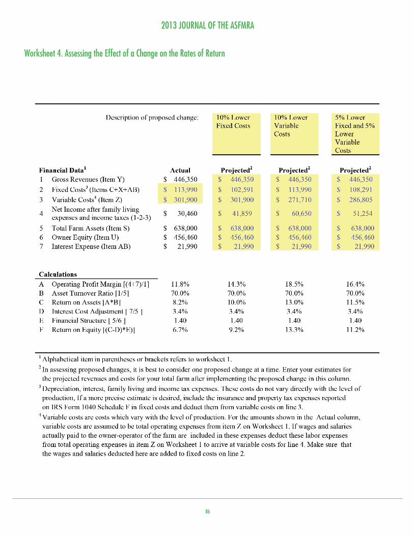
The DuPont Financial Analysis Program is embedded in Worksheet 4 and enables the user to evaluate the impact on the return on equity (ROE) of each of three alternatives being considered for improving financial performance. The numbers used for Worksheet 4 are transferred from the previous worksheets, but the costs do need to be separated into fixed and variable classes. It should be noted that one fixed cost included in the spreadsheet is the withdrawal for family living expenses. Such a designation is not normally made in economic and finance textbooks. However, the family will pay family living expenses regardless of the level of production, so it does satisfy the definition often used for a fixed cost. For practical purposes, the withdrawal for family living expenses is a fixed cost. Revised numbers for each alternative evaluated are then entered and the result is available immediately.

BreakevenBreak-even revenue at the firm level can be calculated by dividing total fixed costs by the contribution to

overhead that is available from each dollar of gross revenue. The contribution to overhead is calculated by subtracting total variable costs as a proportion of gross revenue (variable costs divided by gross revenue) from 1.0 (gross revenue divided by gross revenue).

New: Worksheet 5 is new and uses the fixed costs, variable costs, and gross revenues calculated from the actual farm data in Worksheet 4 to calculate the break-even revenue for the business. Also, a graph is provided that illustrates the original break-even point for the firm and allows the user to observe graphically how that break-even point changes due to changes in gross revenue and operating expenses.

A second break-even amount is also calculated, which includes not only the fixed costs listed above, but also principal payments on term loans, loss carryover amounts and replacement amounts for capital, such as machinery and equipment. This is referred to in the spreadsheet as break-even revenue plus additional needs. The second break-even amount is calculated to determine the point at which all fixed costs, including loan payments on term debt can be met. This measure will be greater than or equal to the original break-even point.

Case Study Example FarmA case study example farm, Frank and Frieda Farmer, is used to illustrate how to enter the data and use the spreadsheet (the five worksheets with the Farmers’ information are included at the end of this article). The example farm used to illustrate the spreadsheet is not intended to represent a typical Indiana farm, but is an example farm that is used


79

to illustrate data entry and the results that can be obtained by using the spreadsheet. Likewise, the results obtained using the example farm should not be generalized, but instead are reported to illustrate the types of analyses that can result from using the spreadsheet, including farm loan repayment sensitivity analysis.

The example farm is a grain farm and has beginning (12/31/20X1) and end-of-year (12/31/20X2) balance sheets, a Schedule F for 20X2 and a Form 4797 that reports the gain from the sale of breeding stock received during 20X2. Information taken from those four forms is entered onto Worksheet 1, along with the number of full-time operators (1) and the family living expenses withdrawn from the farm ($65,000) during 20X2. The accrual-adjusted gross farm revenue, operating expenses, EBITDA, interest expense and net farm income from operations are calculated by the spreadsheet and shown on lines Y-through AC. Net farm income from operations using the accrual-adjusted income statement is then $95,460 and not $19,775 as would be the amount reported on the Schedule F of the federal income tax return.

Next, thirteen financial measures are calculated using numbers from Worksheet 1 and presented on Worksheet 2, along with benchmarks for a Midwest grain farm. The benchmarks used in the worksheet are the medians for Illinois FBFM (Farm Business and Farm Management) grain farms four-year average for 2007-2010 with the exception of the working capital to gross revenues ratio that is obtained from the FINBIN Farm Financial Database for Minnesota farms in 2010. Of course, the benchmarks could

come from other farm record-keeping programs, prior-year financial performance ratios, and other sources as determined by the user. The spreadsheet compares the thirteen financial measures for the example farm to the benchmarks and indicates whether each measure is strong, weak, or neutral compared to the benchmark. As can be seen by reviewing Worksheet 2, one measure for the case study farm is rated strong; whereas, ten are rated weak and two are rated neutral. A neutral rating indicates the results for “Your Farm” fall within a range from 10 percent lower to 10 percent higher than the benchmark.

The troubleshooting procedure for improving financial performance should focus first on those measures that are weaker than the benchmarks. Frank and Frieda Farmer’s rate of return on equity is weaker than the benchmark. This appears to be due in part to a weaker operating profit margin ratio. The asset turnover ratio, which is another primary driver of financial performance on the operating side of the business, is stronger than the benchmark. The weaker operating profit margin ratio indicates that Frank and Frieda could improve the farm’s financial performance by focusing on ways to decrease expenses without reducing revenues. But, their rate of return on equity is also influenced by the financial structure of the farm and it too is weaker than the benchmark. Corrective actions that increase the operating profit margin ratio will increase the rate of return on equity. Reducing leverage, on the other hand, will reduce the rate of return on equity. Increasing leverage by borrowing more will only marginally increase the rate of return on equity unless operating profitability is


80

first increased. So, reducing operating expenses is where the Farmers should focus their efforts to improve the farm’s financial performance. The user can use the list of possible courses of action in Table 6 of the manual describing the spreadsheet (Miller et al., 2012) to identify possible alternatives to evaluate.

The numbers used to complete Worksheet 3 are transferred from Worksheet 1, except for the off-farm income, scheduled principal and interest payments on term debt, carryover operating losses, and funds needed for capital replacement, which the farm operator must input. The term debt coverage ratio (4.21 or 421%) and the capital debt repayment margin ($48,460) are calculated by the spreadsheet. As can be seen, the replacement margin coverage ratio (2.11 or 211%) is indeed smaller than the coverage ratio, since $15,000 was spent for capital replacement.

At the bottom of Worksheet 3, the years to repay term debt and interest rate are entered for a potential loan request, seven and six percent, respectively. The percent of gross income/revenue to retain as a safety margin was entered as five percent, providing a cash reserve safety margin of $22,318. This indicates that the amount of replacement margin available to service new term debt is $11,142 ($33,460 - $22,318). The spreadsheet then calculates the additional term debt that can be serviced with $11,142 of replacement margin available annually, which is $62,202.

The profitability linkage model for Frank and Frieda is automatically calculated and reported as

the actual column on Worksheet 4. To illustrate how to use the profitability linkage model, three alternatives are evaluated: reducing fixed costs by ten percent; reducing variable costs by ten percent; and reducing each of the two types of costs by five percent. As can be seen from the results, the alternative yielding the highest return on equity is to lower variable costs by 10 percent, followed by reducing the fixed and variable costs by 5 percent each.

Additional alternatives can be evaluated by changing a limited number of entries and then comparing the results to the original situation. It should be noted the three alternatives evaluated for Frank and Frieda Farmer were the result of changing only four data entries: one each for alternatives 1 and 2; and two for alternative 3. A desirable feature of the spreadsheet is the number of alternatives that can be evaluated by changing few data entries.

After the data have been changed for the first two alternatives, the break-even for the firm is calculated. The break-even revenue for the farm in 20X2 was $352,234 (Line C, Worksheet 5). This figure changes to $426,395 (Line D, Worksheet 5) when the additional funds needed for annual principal payments on term debt, cash needed to repay unpaid operating debt from a prior period, and cash used to replace capital were included. When variable costs are reduced 10 percent, the original break-even revenue amounts decrease from $352,234 and $426,395 to $291,341 and $352,681, respectively.


81

Final CommentsSeveral farm financial analysis programs are available and provide a comprehensive and thorough analysis of an agricultural business. However, one of the greatest challenges faced by farm and ranch managers and their lenders is to find a program

that provides a thorough financial analysis, uses data managers have in their possession, is simple to use, and is affordable. A farm financial analysis spreadsheet is available for no charge at www.agecon.purdue.edu/files/EC712.xlsx.


82

References

Barnard, F. L. and M. Boehlje, (1998-1999). “The Financial Troubleshooting of Farm Businesses: A Diagnostic and Evaluation System (DES).” Journal of the American Society of Farm Managers and Rural Appraisers: 6-14.

Barnard, F. L. and M. Boehlje, (December 2003). “Worksheets That Work for Measuring and Assessing Farm Financial Performance.” Journal of Extension. Volume 41, Number 6.

Barnard, F. L. and M. Boehlje, (2004). “Using Farm Financial Standards Council Recommendations in the Profitability Linkage Model: The ROA Dilemma.” Journal of the American Society of Farm Managers and Rural Appraisers: 7-11.

Barnard, F. L, P. N. Ellinger and C. Wilson, (2010). “Measurement Issues in Assessing Farm Profitability through Cash Tax Returns,” Journal of the American Society of Farm Managers and Rural Appraisers: 218-229.

2011 FINBIN Report on Minnesota Farm Finances, (April 2012).http://www.cffm.umn.edu/Publications/pubs/FarmMgtTopics/2011MinnesotaFarm FinancialUpdate.pdf.

Financial Characteristics of Illinois FBFM Grain Farms. The Center for Farm and Rural Business Finance, University of Illinois at Urbana-Champaign (2010).

Financial Guidelines for Agricultural Producers: Recommendations of the Farm Financial Council (Revised). (January 2008).

Miller, A., C. Dobbins, M. Boehlje, F. Barnard and N. Olynk, (July 2012). Farm Business Management for the 21st Century: Measuring and Analyzing Farm Financial Performance. Department of Agricultural Economics, Purdue University Cooperative Extension Service EC-712.

Wilson, C., F. Barnard and M. Boehlje. (2007). “A Financial Analysis Program That Will PASS the Farm Manager “Interest Test.” Journal of the American Society of Farm Managers and Rural Appraisers: 34-43.


83

Worksheet 1. Input Information


84

Worksheet 2. Financial Position and Performance Ratios1


85

Worksheet 3. Repayment Capacity Ratios and Measures


86

Worksheet 4. Assessing the Effect of a Change on the Rates of Return


87

Worksheet 5. Determining Break-even Gross Revenues

new features added to the purdue farm financial …ageconsearch.umn.edu/bitstream/161490/2/382a...

Documents