new extended generalized kudryashov method for solving

https://doi.org/10.15388/namc.2020.25.17203Nonlinear Analysis: Modelling and Control, Vol. 25, No. 4, 598–617

eISSN: 2335-8963ISSN: 1392-5113

New extended generalized Kudryashov method forsolving three nonlinear partial differential equations

Elsayed M.E. Zayed, Reham M.A. Shohib, Mohamed E.M. Alngar

Mathematics Department, Faculty of Science, Zagazig University,Zagazig, [email protected]; [email protected];[email protected]

Received: February 18, 2019 / Revised: July 23, 2019 / Published online: July 1, 2020

Abstract. New extended generalized Kudryashov method is proposed in this paper for the firsttime. Many solitons and other solutions of three nonlinear partial differential equations (PDEs),namely, the (1+1)-dimensional improved perturbed nonlinear Schrödinger equation with anti-cubicnonlinearity, the (2+1)-dimensional Davey–Sterwatson (DS) equation and the (3+1)-dimensionalmodified Zakharov–Kuznetsov (mZK) equation of ion-acoustic waves in a magnetized plasma havebeen presented. Comparing our new results with the well-known results are given. Our results inthis article emphasize that the used method gives a vast applicability for handling other nonlinearpartial differential equations in mathematical physics.

Keywords: solitary solutions, a new extended generalized Kudryashov method, the improvedperturbed nonlinear Schrödinger equation with anti-cubic nonlinearity, Davey–Sterwatson (DS)equation, the modified Zakharov–Kuznetsov (mZK) equation of ion-acoustic waves in a magnetizedplasma.

1 Introduction

It is well known that nonlinear complex physical phenomena are related to nonlinearpartial differential equations (NLPDEs), which are implicated in many fields from physicsto biology, chemistry, mechanics, engineering, etc. As mathematical models of the phe-nomena, the investigations of exact solutions of NLPDEs will help one to understand thesephenomena better. In the past several decades, many significant methods for obtainingexact solutions of NLPDEs have been showed, such as the sine-cosine method [3, 5, 18,44], the modified simple equation method [2,13,27,28,40,43], the soliton ansatz method[6–8, 15, 16, 24, 32], the (G′/G)-expansion method [4, 12, 20, 21, 42], the generalizedKudryashov method [25,30,41], the modified transformed rational function method [38],the Lie symmetry method [29,34], the travelling wave hypothesis [14,33,39], the extendedtrial equation method [9–11, 22, 23, 31] and so on.

c© 2020 Authors. Published by Vilnius University PressThis is an Open Access article distributed under the terms of the Creative Commons Attribution Licence,which permits unrestricted use, distribution, and reproduction in any medium, provided the original author andsource are credited.

mailto:[email protected]



https://www.vu.lt/leidyba/en/

https://creativecommons.org/licenses/by/4.0/

New extended generalized Kudryashov method 599

The objective of this article is to use a new extended generalized Kudryashov method,for the first time, to construct new exact solutions of the following three nonlinear partialdifferential equations (PDEs).

(I) The (1+1)-dimensional improved perturbed nonlinear Schrödinger equation withanti-cubic nonlinearity [17]:

iEt + aExt + bExx +

(b1|E|4

+ b2|E|2 + b3|E|4)E

= i[αEx + λ(|E|2E)x + υ1

(|E|2

)xE], (1)

where i =√−1, a, b, b1, b2, b3, α, λ and υ1 are real constants. The independent variables

x and t represent spatial and temporal variables, respectively. The dependent variableE(x, t) is the complex valued wave profile for the (1 + 1)-dimensional improved per-turbed nonlinear Schrödinger equation with anti-cubic nonlinearity. Here the coefficientsa and b represent the improved term that introduces stability to the NLS equation and theusual group velocity dispersion (GVD), respectively. The nonlinearities stem out fromthe coefficients of bj for j = 1, 2, 3, where b1 gives the effect of anti-cubic nonlinearity,b2 is the coefficient of Kerr law nonlinearity, and b3 is the coefficient of pseudo-quinticnonlinearity, respectively. The parameters α and λ represent the intermodal dispersion andthe self-steepening perturbation term, respectively. Finally, υ1 is the nonlinear dispersioncoefficient. If b1 = 0, there is no anti-cubic nonlinearity. which has been discussed in [17]using the soliton ansatz method.

(II) The (2 + 1)-dimensional Davey–Sterwatson (DS) equation [19, 26, 35, 45]:

iut +1

2σ2(uxx + σ2uyy

)+ λ|u|2u− uvx = 0,

vxx − σ2vyy − 2λ(|u|2)x= 0,

(2)

where λ is a real constant. The case σ = 1 is called the DS-I equation, while σ = iis the DS-II equation. The parameter λ characterizes the focusing or defocusing case.The Davey–Stewartson I and II are two well-known examples of integrable equations intwo space dimensions, which arise as higher dimensional generalizations of the nonlinearSchrodinger (NLS) equation [19]. They appear in many applications, for example, inthe description of gravity–capillarity surface wave packets in the limit of the shallowwater. Davey and Stewartson first derived their model in the context of water waves frompurely physical considerations. In the context, u(x, y, t) is the amplitude of a surfacewave packet, while v(x, y) represents the velocity potential of the mean flow interactingwith the surface wave [19]. Equation (2) has been discussed in [35] using the numericalschemes method, in [45] – using the homotopy perturbation method, in [19] – using themultiple scales method and in [26] – using the first-integral method.

(III) The (3 + 1)-dimensional modified ZK equation of ion-acoustic waves in a mag-netized plasma [36]:

16

(∂q

∂t− c ∂q

∂x

)+ 30q1/2

∂q

∂x+∂3q

∂x3+

∂

∂x

(∂2

∂y2+

∂2

∂z2

)q = 0, (3)

Nonlinear Anal. Model. Control, 25(4):598–617

https://doi.org/10.15388/namc.2020.25.17203

600 E.M.E. Zayed et al.

where c is a positive real constant. Equation (3) has been discussed by Munro and Parkes[36], where they showed that if the electrons are nonisothermal, then the govering equa-tion of the ZK equation is a modified form refereed to as the mZK equation (3), also theyshowed that the reductive perturbation method leads to a modified Zakharov–Kuznetsov(mZK) equation.

This article is organised as follows: In Section 2, we give the description of a newextended generalized Kudryashov method for the first time. In Sections 3, 4 and 5, wesolve Eqs. (1), (2) and (3) using the proposed method described in Section 2. In Section 6,the graphical representations for some solutions of Eqs. (1), (2) and (3) are plotted. InSections 7, conclusions are illustrated. To our knowledge, Eqs. (1), (2) and (3) are notdiscussed before using the proposed method obtained in the next section.

2 Description of a new extended generalized Kudryashov method

Consider the following nonlinear PDE:

P (u, ux, uy, uz, ut, uxx, uyy, uzz, uxy, utt, . . . ) = 0, (4)

where P is a polynomial in u and its partial derivatives in which the highest-order deriva-tives and the nonlinear terms are involved. According to the well-known generalizedKudryashov method [25, 30, 41] and with reference to [38], we can propose the mainsteps of a new extended generalized Kudryashov method for the first time as follows:

Step 1. We use the traveling wave transformation

u(x, y, z, t) = u(ξ), ξ = l1x+ l2y + l3z − l4t,

where l1, l2, l3 and l4 are a nonzero constants, to reduce Eq. (4) to the following nonlinearordinary differential equation (ODE):

H(u, u′, u′′, . . . ) = 0, (5)

where H is a polynomial in u(ξ) and its total derivatives u′(ξ), u′′(ξ) and so on, where′ = d/dξ.

Step 2. We assume that the formal solution of the ODE (5) can be written in thefollowing rational form:

u(ξ) =

∑si=0 αiQ

i(ξ)∑mj=0 βjQ

j(ξ)=A[Q(ξ)]

B[Q(ξ)], (6)

where A[Q(ξ)]=∑si=0 αiQ

i(ξ) and B[Q(ξ)]=∑mj=0 βjQ

j(ξ) such that αs and βm 6=0and

Q(ξ) =

[1

1± expa(pξ)

]1/p, (7)

http://www.journals.vu.lt/nonlinear-analysis



where expa(pξ) = apξ and p is a positive integer. The function Q is the solution of thefirst-order differential equation

Q′(ξ) =[Qp+1(ξ)−Q(ξ)

]ln a, 0 < a 6= 1. (8)

From (6) and (8) we have

u′(ξ) = Q(Qp − 1

)[A′B −AB′B2

]ln a,

u′′(ξ) = Q(Qp − 1

)[(p+ 1)Qp − 1

][A′B −AB′B2

]ln2a

+Q2(Qp − 1

)2[B(A′′B −AB′′)− 2A′B′B + 2AB′2

B3

]ln2a,

(9)

and so on.

Step 3. We determine the positive integers values m and s in (6) by using the homo-geneous balance method as follows: If D(u) = s −m,D(u′) = s −m + p,D(u′′) =s−m+ 2p, then we have

D[uru(q)

]= (s−m)(r + 1) + pq. (10)

Step 4. We substitute (6), (8) and (9) into Eq. (5) and equate all the coefficients of Qi

(i = 0, 1, 2, . . . ) to zero. We obtain a system of algebraic equations, which can be solvedusing the Maple, to find the αi (i = 0, 1, . . . , s), βj (j = 0, 1, . . . ,m), l1, l2, l3 and l4.Consequently, we can get the exact solutions of Eq. (4).

The obtained solutions will be depended on the symmetrical hyperbolic Fibonaccifunctions given in [1] and [37]. The symmetrical Fibonacci sine, cosine, tangent andcotangent functions are defined as

sFs(ξ) =aξ − a−ξ√

5, cFs(ξ) =

aξ + a−ξ√5

,

(11)

tanFs(ξ) =aξ − a−ξ

aξ + a−ξ, cotFs(ξ) =

aξ + a−ξ

aξ − a−ξ,

sFs(ξ) =2√5sh[ξ ln a], cFs(ξ) =

2√5

ch[ξ ln a],

tanFs(ξ) = tanh[ξ ln a], cotFs(ξ) = coth[ξ ln a].

3 On solving Eq. (1)(1)(1) using the new extended generalized Kudryashovmethod

In this section, we use the above method describing in Section 2 for solving Eq. (1). Tothis aim, we assume that Eq. (1) has the formal solution

E(x, t) = ψ(ξ)ei[χ(ξ)−ωt], ξ = kx− εt, (12)




where ψ(ξ) and χ(ξ) are real functions of ξ, while ω, k and ε are real constants. Substi-tuting (12) into Eq. (1) and separating the real and the imaginary parts, we have the twononlinear ODEs:

(ε+ akω + αk)χ′ψ + ωψ + b1ψ−3 + b2ψ

3 + b3ψ5 + k(bk − aε)ψ′′

− k(bk − aε)χ′2ψ + kλχ′ψ3 = 0 (13)

and−(ε+ αk + akω)ψ′ + 2k(bk − aε)χ′ψ′ + k(bk − aε)χ′′ψ− k[3λ+ 2υ1]ψ

2ψ′ = 0. (14)

To solve the above coupled pair of Eqs. (13) and (14), we introduce the ansatz:

χ′(ξ) = βψ2(ξ) + γ, (15)

where β and γ are constants. Inserting (15) into Eq. (14), we obtain

β =3λ+ 2υ14(kb− aε)

and γ =ε+ αk + akω

2k(bk − aε). (16)

Substituting (15) along with (16) into Eq. (13), we have the nonlinear ODE

ψ3ψ′′ +A1 +A2ψ4 +A3ψ

6 +A4ψ8 = 0, (17)

where the coefficients A1, A2, A3 and A4 are given by

A1 =b1

k(bk − aε), A2 =

(ε+ αk + akω)2 + 4kω(bk − aε)4k2(bk − aε)2

,

A3 =2b2(bk − aε) + λ(ε+ αk + akω)

2k(bk − aε)2,

A4 =16b3(bk − aε)− k(3λ+ 2υ1)

2 + 4kλ(3λ+ 2υ1)

16k(bk − aε)2,

where k(bk − aε) 6= 0. Settingψ2(ξ) = g(ξ), (18)

where g(ξ) is a positive function of ξ. Substituting (18) into (17), we have the newequation

2gg′′ − g′2 + 4(A1 +A2g

2 +A3g3 +A4g

4)= 0. (19)

By balancing gg′′ with g4 in (19), the following formula is obtained:

2(s−m) + 2p = 4(s−m) =⇒ s = m+ p.

Let us now discuss the following cases.




Case 1. If we choose p = 1 and m = 1, then s = 2. Thus, we deduce from (6) that

ψ(ξ) =α0 + α1Q(ξ) + α2Q

2(ξ)

β0 + β1Q(ξ), (20)

where α0, α1, α2, β0 and β1 are real constants to be determined such that α2 and β1 6= 0.Substituting (20) along with (8) into Eq. (19), collecting the coefficients of each power ofQi (i = 0, 1, . . . , 8) and setting each of these coefficients to zero, we obtain a system ofalgebraic equations, which can be solved using Maple, we obtain the following results.

Result 1.

A1 =α20 ln

2 a (β21 − 2β0β1 + β2

0)

4β20β

21

, A2 =− ln2a (β2

1 − 6β0β1 + 6β20)

4β21

,

A3 =β20 ln

2a (2β0 − β1)α0β2

1

, A4 =−3β4

0 ln2a

4α20β

21

,

β0 = β0, β1 = β1, α0 = α0, α1 = 0, α2 =−β2

1α0

β20

.

(21)

In this case, from (7), (12), (18), (20) and (21) we deduce that Eq. (1) has the solution

E(x, t) =

{α0

β0− α0β1

β20

1

1± aξ

}1/2

e(i[χ(ξ)−ωt]). (22)

From (22) we deduce that Eq. (1) has the dark soliton solution

E(x, t) =

{α0

β0− α0β1

2β20

[1− tanh

ξ ln a

2

]}1/2

e(i[χ(ξ)−ωt])

and the singular soliton solution

E(x, t) =

{α0

β0− α0β1

2β20

[1− coth

ξ ln a

2

]}1/2

e(i[χ(ξ)−ωt]),

provided α0β0 > 0 and α0β1 < 0.

Result 2.

A1 =−3[9A4

3 + 8A4(2A4 ln2a+ 3A2

3) ln2a]

4096A34

, A2 =9A2

3 + 4A4 ln2a

32A4,

α0 = 0, α1 =−β1[2 ln a

√−3A4 + 3A3]

8A4, α2 =

β1 ln a√−3A4

2A4,

β0 = 0, β1 = β1,

(23)

provided A4 < 0. In this case, from (7), (12), (18), (20) and (23) we deduce that Eq. (1)has the solution

E(x, t) =

{−3A3

8A4+

ln a√−3A4

4A4

[1∓ aξ

1± aξ

]}1/2

e(i[χ(ξ)−ωt]). (24)





E(x, t) =

{−3A3

8A4− ln a

√−3A4

4A4tanh

ξ ln a

2

}1/2

e(i[χ(ξ)−ωt]) (25)

and the singular soliton solution

E(x, t) =

{−3A3

8A4− ln a

√−3A4

4A4coth

ξ ln a

2

}1/2

e(i[χ(ξ)−ωt]),

provided A4 < 0 and A3 > 0.

Case 2. If we choose p = 2 and m = 2, then s = 4, thus, we deduce from (6) that

g(ξ) =α0 + α1Q(ξ) + α2Q

2(ξ) + α3Q3(ξ) + α4Q

4(ξ)

β0 + β1Q(ξ) + β2Q2(ξ), (26)

where α0, α1, α2, α3, α4, β0, β1 and β2 are real constants to be determined such thatα4 and β2 6= 0. Substituting (26) along with (8) into Eq. (19), collecting the coefficientsof each power of Qi (i = 0, 1, . . . , 16) and setting each of these coefficients to zero, weobtain a set of algebraic equations, which can be solved by Maple, to get the followingresults.

Result 1.

α0 = 0, α1 = α1, α2 =α1β2β1

, α3 =3β1 ln a√−3A4

, α4 =3β2 ln(a)√−3A4

,

A1 =−α2

1[6A4α1β1 ln a+ [A4α21 − 3β2

1 ln2a]√−3A4]

3β41

√−3A4

,

A2 =6A4α1β1 ln a+ [2A4α

21 − β2

1 ln2a]√−3A4

β21

√−3A4

,

A3 =−4A4[3β1 ln a+ 2α1

√−3A4]

3β1√−3A4

, β0 = 0, β1 = β1, β2 = β2,

(27)


E(x, t) =

{α1

β1+

3 ln a√−3A4

1

1± a2ξ

}1/2

e(i[χ(ξ)−ωt]).

Equation (1) has the symmetrical Fibonacci cotangent function solutions

E(x, t) =

{α1

β1+

3 ln a

2√−3A4

[1− tanFs(ξ)

]}1/2

e(i[χ(ξ)−ωt]) (28)

and

E(x, t) =

{α1

β1+

3 ln a

2√−3A4

[1− cotFs(ξ)

]}1/2

e(i[χ(ξ)−ωt]). (29)





E(x, t) =

{α1

β1+

3 ln a

2√−3A4

[1− tanh(ξ ln a)

]}1/2

e(i[χ(ξ)−ωt]), (30)

and from (29) we deduce that Eq. (1) has the singular soliton solution

E(x, t) =

{α1

β1+

3 ln a

2√−3A4

[1− coth(ξ ln a)

]}1/2

e(i[χ(ξ)−ωt]), (31)

provided A4 < 0 and α1β1 > 0.

Result 2.

α0 = 0, α1 = 0, α2 =−β2(4 ln a

√−3A4 + 3A3)

8A4, α3 = 0,

α4 =β2 ln a

√−3A4

A4, β0 = 0, β1 = 0, β2 = β2,

A1 =−3[256A2

4 ln4(a) + 96A2

3A4 ln2(a) + 9A4

3]

4096A34

,

A2 =16A4 ln

2(a) + 9A23

32A4,

(32)


E(x, t) =

{−3A3

8A4+

ln a

2

√−3A4

1∓ a2ξ

1± a2ξ

}1/2

e(i[χ(ξ)−ωt]).

Equation (1) has the symmetrical Fibonacci cotangent function solutions

E(x, t) =

{−3A3

8A4− ln a

2

√−3A4

tanFs(ξ)

}1/2

e(i[χ(ξ)−ωt]) (33)

and

E(x, t) =

{−3A3

8A4− ln a

2

√−3A4

cotFs(ξ)

}1/2

e(i[χ(ξ)−ωt]). (34)


E(x, t) =

{− 3A3

8A4− ln a

2

√−3A4

tanh(ξ ln a)

}1/2

e(i[χ(ξ)−ωt]),

and from (34) we deduce that Eq. (1) has the singular soliton solution

E(x, t) =

{−3A3

8A4− ln a

2

√−3A4

coth(ξ ln a)

}1/2

e(i[χ(ξ)−ωt]),

provided A4 < 0 and A3 > 0. Simliarly, we can find many other solutions by choosinganother values for s, m and p.






u(x, y, t) = u(ξ)eiη(x,y,t), v(x, y) = v(ξ), (35)

andξ = x− 2αy + αt, η(x, y, t) = αx+ y + kt+ l, (36)

where u(ξ), η(x, y, t) and v(ξ) are all real functions, while α, k and l are real constants.Substituting (35) and (36) into Eq. (2) yield the following system of ODEs:

σ2(1 + 4σ2α2

)u′′(ξ) + 2λu3(ξ)−

(2k + σ2α2 + σ4

)u(ξ)

− 2u(ξ)v′(ξ) = 0, (37)(1− 4σ2α2)v′′(ξ) = 2λ

[u2(ξ)

]′. (38)

Integrating (38) with respect to ξ, we obtain

v′(ξ) =2λ

(1− 4σ2α2)u2(ξ) + ε, (39)

where ε is the constant of integration, and α2 6= ±1/4. Substituting (39) into (37), wehave

σ2(1 + 4σ2α2

)u′′(ξ) + 2λ

[1− 2

(1− 4σ2α2)

]u3(ξ)

−(2k + σ2α2 + σ4 + 2ε

)u(ξ) = 0. (40)

By balancing u′′ with u3 in (40), the following formula is obtained:

(s−m) + 2p = 3(s−m) =⇒ s = m+ p.



u(ξ) =α0 + α1Q(ξ) + α2Q

2(ξ)

β0 + β1Q(ξ), (41)

where α0, α1, α2, β0 and β1 are real constants to be determined such that α2 and β1 6= 0.Substituting (41) along with (8) into Eq. (40), collecting the coefficients of each power ofQi (i = 0, 1, . . . , 6) and setting each of these coefficients to zero, we obtain a system ofalgebraic equations, which can be solved by Maple, we obtain the following results.




Result 1.

ε = −1

2

[2k + σ2

(α2 + σ2

)− σ2 ln2a

(1 + 4σ2α2

)],

α0 = 0, α1 = α1, α2 = −α1,

β0 =−α1

2σ ln a

√λ

(1− 4σ2α2), β1 =

α1

σ ln a

√λ

(1− 4σ2α2),

(42)

provided (1 − 4σ2α2)λ > 0. In this case, from (7), (35), (36), (41) and (42) we deducethat Eq. (2) has the solution

u(x, y, t) =

(±2σ ln a

√(1− 4σ2α2)

λ

aξ

1− a2ξ

)eiη(x,y,t). (43)

From (43) we deduce that Eq. (2) has the singular solitary wave solution

u(x, y, t) =

(∓σ ln a

√(1− 4σ2α2)

λcsch[ξ ln a]

)eiη(x,y,t). (44)

Result 2.

ε = −1

4

[4k + 2σ2

(α2 + σ2

)+ σ2 ln2a

(1 + 4σ2α2

)],

α0 = 0, α1 =−β1σ ln a

2

√(1− 4σ2α2)

λ,

α2 = β1σ ln a

√(1− 4σ2α2)

λ, β0 = 0, β1 = β1,

(45)


u(x, y, t) =

(σ ln a

2

√(1− 4σ2α2)

λ

1∓ aξ

1± aξ

)eiη(x,y,t). (46)

From (46) we deduce that Eq. (2) has the shock wave solution

u(x, y, t) =

(−σ ln a

2

√(1− 4σ2α2)

λtanh

ξ ln a

2

)eiη(x,y,t)

and the singular solitary wave solution

u(x, y, t) =

(−σ ln a

2

√(1− 4σ2α2)

λcoth

ξ ln a

2

)eiη(x,y,t).


u(ξ) =α0 + α1Q(ξ) + α2Q

2(ξ) + α3Q3(ξ) + α4Q

4(ξ)

β0 + β1Q(ξ) + β2Q2(ξ), (47)




where α0, α1, α2, α3, α4, β0, β1 and β2 are real constants to be determined such thatα4 and β2 6= 0. Substituting (47) along with (8) into Eq. (40), collecting the coefficientsof each power of Qi (i = 0, 1, . . . , 12) and setting each of these coefficients to zero, weobtain a set of algebraic equations, which can be solved by Maple, to get the followingresults.

Result 1.

ε = −1

2

[2k + σ2

(α2 + σ2

)+ 8σ2 ln2a

(1 + 4σ2α2

)],

α0 = β2σ ln a

√(1− 4σ2α2)

λ, α1 = 0,

α2 = −2β2σ ln a√

(1− 4σ2α2)

λ,

α3 = 0, α4 = 2β2σ ln a

√(1− 4σ2α2)

λ,

β0 =−12β2, β1 = 0, β2 = β2,

(48)


u(x, y, t) =

(2σ ln a

√(1− 4σ2α2)

λ

1 + a4ξ

1− a4ξ

)eiη(x,y,t). (49)


u(x, y, t) =

(−2σ ln a

√(1− 4σ2α2)

λcoth[2ξ ln a]

)eiη(x,y,t). (50)

Result 2.

ε = −1

2

[2k + σ2

(α2 + σ2

)− 4σ2 ln2a

(1 + 4σ2α2

)],

α0 = 0, α1 = 0, α2 = −2β2σ ln a√

(1− 4σ2α2)

λ,

α3 = 0, α4 = 2β2σ ln a

√(1− 4σ2α2)

λ,

β0 = −1

2β2, β1 = 0, β2 = β2,

(51)


u(x, y, t) = ∓(4σ ln a

√(1− 4σ2α2)

λ

a2ξ

1− a4ξ

)eiη(x,y,t). (52)





u(x, y, t) = ±(2σ ln a

√(1− 4σ2α2)

λcsch[2ξ ln a]

)eiη(x,y,t).

Similarly, we can find many other solutions by choosing another values for s, m and p.



q(x, y, z, t) = B(ξ), ξ = kx+ ly + ρz − ωt, (53)

where B(ξ) is a real function, while k, l, ρ and ω are real constants, to reduce Eq. (3) intothe nonlinear ODE

− 16(ω + kc)B′(ξ) + 30kB1/2(ξ)B′(ξ) + k(k2 + l2 + ρ2

)B′′′(ξ) = 0, (54)

where ′ = d/dξ. Integrating Eq. (54) once with respect to ξ, we have

−16(ω + kc)B(ξ) + 20kB3/2(ξ) + k(k2 + l2 + ρ2

)B′′(ξ) + ε = 0,

where ε is the constant of integration. Setting

B(ξ) = H2(ξ), (55)

we get the equation

−16(ω+kc)H2(ξ)+20kH3(ξ)+2k(k2+l2+ρ2

)[H ′2(ξ)+H(ξ)H ′′(ξ)

]+ε = 0. (56)

By balancing HH ′′ with H3 in (56), the following formula is obtained:

2(s−m) + 2p = 3(s−m) =⇒ s = m+ 2p.


Case 1. If we choose p = 1 and m = 1, then s = 3, Thus, we deduce from (6) that

H(ξ) =α0 + α1Q(ξ) + α2Q

2(ξ) + α3Q3(ξ)

β0 + β1Q(ξ), (57)

where α0, α1, α2, α3, β0 and β1 are real constants to be determined, such that α3 andβ1 6= 0. Substituting (57) along with (8) into Eq. (56), collecting the coefficients of eachpower of Qi (i = 0, 1, . . . , 10) and setting each of these coefficients to zero, we obtaina system of algebraic equations, which can be solved by Maple, we obtain the followingresults.




Result 1.

α0 = 0, α1 =−β1(k2 + l2 + ρ2) ln2a

6, α2 = β1(k

2 + l2 + ρ2) ln2a,

α3 = −β1(k2 + l2 + ρ2) ln2a, ω =−k[(k2 + l2 + ρ2) ln2a+ 4c]

4,

ε =−k[(k2 + l2 + ρ2) ln2a]3

54, β0 = 0, β1 = β1.

(58)


B(ξ) =

[−(k2 + l2 + ρ2) ln2a

6

(1∓ 6aξ

(1± aξ)2

)]2. (59)

From (59) we deduce that Eq. (3) has the solitary wave solution

B(ξ) =(k2 + l2 + ρ2)2 ln4(a)

36

[1− 3

2sech2

ξ ln a

2

]2(60)


B(ξ) =(k2 + l2 + ρ2)2 ln4a

36

[1 +

3

2csch2

ξ ln a

2

]2,

where ξ = kx+ ly + ρz + (k/4)[(k2 + l2 + ρ2) ln2a+ 4c]t.Result 2.

α0 = 0, α1 = 0, α2 = β1(k2 + l2 + ρ2) ln2a,

α3 = −β1(k2 + l2 + ρ2

)ln2a, ω =

k[(k2 + l2 + ρ2) ln2a− 4c]

4,

ε = 0, β0 = 0, β1 = β1.

(61)


B(ξ) =(k2 + l2 + ρ2

)2ln4a

(aξ

(1± aξ)2

)2

. (62)


B(ξ) =(k2 + l2 + ρ2)2 ln4a

16sech4

ξ ln a

2


B(ξ) =(k2 + l2 + ρ2)2 ln4a

16csch4

ξ ln a

2,

where ξ = kx+ ly + ρz − (k/4)[(k2 + l2 + ρ2) ln2a− 4c]t.





H(ξ) =α0 + α1Q(ξ) + α2Q

2(ξ) + α3Q3(ξ) + α4Q

4(ξ) + α5Q5(ξ)

β0 + β1Q(ξ), (63)

where α0, α1, α2, α3, α4, α5, β0 and β1 are real constants to be determined, such thatα5 and β1 6= 0. Substituting (63) along with (8) into Eq. (56), collecting the coefficientsof each power of Qi (i = 0, 1, . . . , 16) and setting each of these coefficients to zero, weobtain a set of algebraic equations, which can be solved by Maple, to get the followingresults.

Result 1.

α0 = −2

3β0(k2+l2+ρ2

)ln2a, α1 = −2

3β1(k

2+l2+ρ2)ln2a, β0 = β0,

β1 = β1, α2 = 4β0(k2+l2+ρ2

)ln2a, α3 = 4β1

(k2+l2+ρ2

)ln2a,

α4 = −4β0(k2+l2+ρ2

)ln2a, α5 = −4β1

(k2+l2+ρ2

)ln2a,

ω = −k[(k2+l2+ρ2

)ln2a+ c

], ε =

−3227

k[(k2+l2+ρ2

)ln2a

]3.

(64)

In this case, (7), (53), (55), (63) and (64) we deduce that Eq. (3) has the solution

B(ξ) =

[−23

(k2 + l2 + ρ2

)ln2a

(1− 6

1± a2ξ+

6

(1± a2ξ)2

)]2.

With the help of (11), Eq. (3) has the symmetrical Fibonacci cotangent function solutions

B(ξ) =1

9

(k2 + l2 + ρ2

)2ln4a

[1− 3 tanFs2(ξ)

]2, (65)

and

B(ξ) =1

9

(k2 + l2 + ρ2

)2ln4a

[1− 3 cotFs2(ξ)

]2. (66)

From (65) we deduce that Eq. (3) has the shock wave solution

B(ξ) =1

9

(k2 + l2 + ρ2)2 ln4a

[1− 3 tanh2(ξ ln a)

]2,

and from (66) we deduce that Eq. (3) has the singular solitary wave solution

B(ξ) =1

9(k2 + l2 + ρ2)2 ln4a

[1− 3 coth2(ξ ln a)

]2,

where ξ = kx+ ly + ρz + k[(k2 + l2 + ρ2) ln2a+ c]t.




Result 2.

α0 = 0, α1 = 0, β0 = β0, β1 = β1,

α2 = 4β0(k2 + l2 + ρ2

)ln2a, α3 = 4β1

(k2 + l2 + ρ2

)ln2a,

α4 = −4β0(k2 + l2 + ρ2

)ln2a, α5 = −4β1

(k2 + l2 + ρ2

)ln2a,

ε = 0, ω = k[(k2 + l2 + ρ2

)ln2a− c

].

(67)


B(ξ) = 16(k2 + l2 + ρ2

)2ln4a

(a2ξ

(1± a2ξ)2

)2

.

With the help of (11), Eq. (3) has the symmetrical Fibonacci cotangent function solutions

B(ξ) =(k2 + l2 + ρ2

)2ln4a

[1− tanFs2(ξ)

]2(68)

andB(ξ) =

(k2 + l2 + ρ2

)2ln4a

[1− cotFs2(ξ)

]2. (69)


B(ξ) =(k2 + l2 + ρ2

)2ln4a sech4[ξ ln a], (70)

and from (69) we deduce that Eq. (3) has the singular solitary wave solution

B(ξ) =(k2 + l2 + ρ2

)2ln4a csch4[ξ ln a],

where ξ = kx+ ly + ρz − k[(k2 + l2 + ρ2) ln2a− c]t.

6 Some graphical representations of some solutions

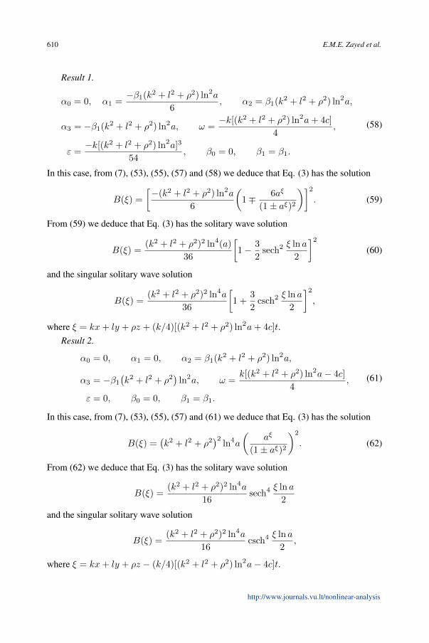
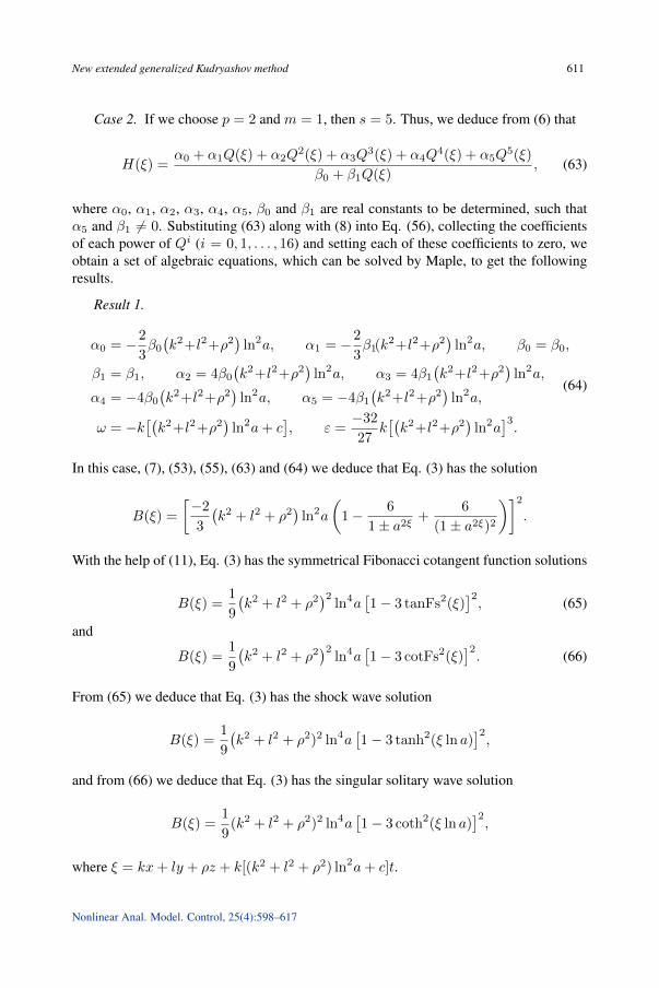
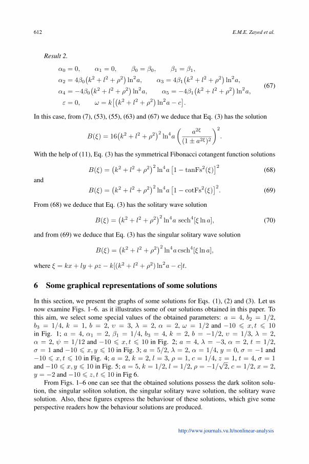
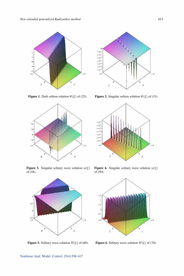
In this section, we present the graphs of some solutions for Eqs. (1), (2) and (3). Let usnow examine Figs. 1–6. as it illustrates some of our solutions obtained in this paper. Tothis aim, we select some special values of the obtained parameters: a = 4, b2 = 1/2,b3 = 1/4, k = 1, b = 2, υ = 3, λ = 2, α = 2, ω = 1/2 and −10 6 x, t 6 10in Fig. 1; a = 4, α1 = 2, β1 = 1/4, b3 = 4, k = 2, b = −1/2, υ = 1/3, λ = 2,α = 2, ψ = 1/12 and −10 6 x, t 6 10 in Fig. 2; a = 4, λ = −3, α = 2, t = 1/2,σ = 1 and −10 6 x, y 6 10 in Fig. 3; a = 5/2, λ = 2, α = 1/4, y = 0, σ = −1 and−10 6 x, t 6 10 in Fig. 4; a = 2, k = 2, l = 3, ρ = 1, c = 1/4, z = 1, t = 4, σ = 1and −10 6 x, y 6 10 in Fig. 5; a = 5, k = 1/2, l = 1/2, ρ = −1/

√2, c = 1/2, x = 2,

y = −2 and −10 6 z, t 6 10 in Fig 6.From Figs. 1–6 one can see that the obtained solutions possess the dark soliton solu-

tion, the singular soliton solution, the singular solitary wave solution, the solitary wavesolution. Also, these figures express the behaviour of these solutions, which give someperspective readers how the behaviour solutions are produced.




Figure 1. Dark soliton solution Ψ(ξ) of (25). Figure 2. Singular soliton solution Ψ(ξ) of (31).

Figure 3. Singular solitary wave solution u(ξ)of (44).

Figure 4. Singular solitary wave solution u(ξ)of (50).

Figure 5. Solitary wave solution H(ξ) of (60). Figure 6. Solitary wave solution H(ξ) of (70).




7 Conclusions

For the first time, we have derived many new exact solutions of the three nonlinear partialdifferential equations (PDEs), namely, the (1 + 1)-dimensional improved perturbed non-linear Schrödinger equation with anti-cubic nonlinearity, the (2+1)-dimensional Davey–Sterwatson (DS) equation and the (3 + 1)-dimensional modified Zakharov–Kuznetsov(mZK) equation of ion-acoustic waves in a magnetized plasma using the new extendedgeneralized Kudryashov method. The obtained solutions will be depended on the symmet-rical hyperbolic Fibonacci functions. Equation (1) is nonlinear optics, where its solutionsin Section 3 are called bright soliton solutions, dark soliton solutions, singular solitonsolutions and trigonometric function solutions, while Eq. (2) is fluid dynamics, and Eq. (3)is plasma physics, where their solutions in Sections 4 and 5 are called solitary wave, shockwave and singular solitary waves. All the solutions obtained in Sections 3–5 will be a goodguide line and great help for a large family of scientists. On comparing our solutions ofthese equations with that obtained in [17, 19, 26, 35, 36, 45], we deduce that our solutionsare new and not reported previously in the literature. Finally, our results in this articlehave been checked using the Maple by putting them back into the original equations (1),(2) and (3).

Acknowledgment. The authors wish to thank the referees for their comments on thispaper.

References

1. A.T. Ali, E.R. Hassan, General Expa-method for nonlinear evolution equations, Appl. Math.Comput., 217(2):451–459, 2010.

2. A.H. Arnous, A. Biswas, M. Asma, M. Belic, Dark and singular solitons in optical meta-materials with anti-cubic nonlinearity by modified simple equation approach, Optoelectron.Adv. Mat., 12(5-6):332–336, 2018.

3. A. Bekir, New exact travelling wave solutions of some complex nonlinear equations, Commun.Nonlinear Sci. Numer. Simul., 14(4):1069–1077, 2009.

4. A. Bekir, B. Ayhan, M.N. Özer, Explicit solutions of nonlinear wave equation systems, Chin.Phys. B, 22(1):010202, 2013.

5. A. Bekir, A.C. Cevikel, New solitons and periodic solutions for nonlinear physical models inmathematical physics, Nonlinear Anal., Real World Appl., 11(4):3275–3285, 2010.

6. A.H. Bhrawy, M.A. Abdelkawy, S. Kumar, S. Johnson, A. Biswas, Solitons and other solutionsto quantum Zakharov–Kuznetsov equation in quantum magneto-plasmas, Indian J. Phys.,87(5):455–463, 2013.

7. A. Biswas, 1-soliton solution of the k (m, n) equation with generalized evolution, Phys. Lett. A,372(25):4601–4602, 2008.

8. A. Biswas, 1-soliton solution of the generalized Zakharov–Kuznetsov equation with nonlineardispersion and time-dependent coefficients, Phys. Lett. A, 373(33):2931–2934, 2009.




9. A. Biswas, Conservation laws for optical solitons with anti-cubic and generalized anti-cubicnonlinearities, Optik, 176:198–201, 2019.

10. A. Biswas, M. Ekici, A. Sonmezoglu, M. Belic, Chirped and chirp-free optical solitons withgeneralized anti-cubic nonlinearity by extended trial function scheme, Optik, 178:636–644,2019.

11. A. Biswas, M. Ekici, A. Sonmezoglu, M. R. Belic, Optical solitons in birefringent fibers havinganti-cubic nonlinearity with extended trial function, Optik, 185:456–463, 2019.

12. A. Biswas, M. Ekici, A. Sonmezoglu, Q. Zhou, A.S. Alshomrani, S.P. Moshokoa, M. Belic,Solitons in optical metamaterials with anti-cubic nonlinearity, Eur. Phys. J. Plus, 133(5):204,2018.

13. A. Biswas, A.J.M. Jawad, Q. Zhou, Resonant optical solitons with anti-cubic nonlinearity,Optik, 157:525–531, 2018.

14. A. Biswas, M. Song, Soliton solution and bifurcation analysis of the Zakharov–Kuznetsov–Benjamin–Bona–Mahoney equation with power law nonlinearity, Commun. Nonlinear Sci.Numer. Simul., 18(7):1676–1683, 2013.

15. A. Biswas, E. Zerrad, 1-soliton solution of the Zakharov–Kuznetsov equation with dual-powerlaw nonlinearity, Commun. Nonlinear Sci. Numer. Simul., 14(9-10):3574–3577, 2009.

16. A. Biswas, E. Zerrad, Solitary wave solution of the Zakharov–Kuznetsov equation in plasmaswith power law nonlinearity, Nonlinear Anal., Real World Appl., 11(4):3272–3274, 2010.

17. Amel. Bouzida, H. Triki, M.Z. Ullah, Q. Zhou, A. Biswas, M. Belic, Chirped optical solitonsin nano optical fibers with dual-power law nonlinearity, Optik, 142:77–81, 2017.

18. A.C. Cevikel, A. Bekir, New solitons and periodic solutions for (2 + 1)-dimensional Davey–Stewartson equations, Chin. J. Phys., 51(1):1–13, 2013.

19. A. Davey, K. Stewartson, On three-dimensional packets of surface waves, Proc. R. Soc. Lond.,A, Math. Phys. Eng. Sci., 338(1613):101–110, 1974.

20. G. Ebadi, A. Biswas, The (G′/G) and 1-soliton solution of the Davey–Stewartson equation,Math. Comput. Modelling, 53(5–6):694–698, 2011.

21. G. Ebadi, A. Mojaver, D. Milovic, S. Johnson, A. Biswas, Solitons and other solutions to thequantum Zakharov–Kuznetsov equation, Astrophys. Space Sci., 341(2):507–513, 2012.

22. M. Ekici, M. Mirzazadeh, A. Sonmezoglu, M.Z. Ullah, Q. Zhou, H. Triki, S.P. Moshokoa,A. Biswas, Optical solitons with anti-cubic nonlinearity by extended trial equation method,Optik, 136:368–373, 2017.

23. M. Ekici, A. Sonmezoglu, Q. Zhou, S.P. Moshokoa, M.Z. Ullah, A.H. Arnous, A. Biswas,M. Belic, Analysis of optical solitons in nonlinear negative-indexed materials with anti-cubicnonlinearity, Opt. Quantum Electron., 50(2):75, 2018.

24. Ö. Güner, A. Bekir, L. Moraru, A. Biswas, Bright and dark soliton solutions of the generalizedZakharov–Kuznetsov–Benjamin–Bona–Mahony nonlinear evolution equation, in Proc. Rom.Acad., Ser. A, Math. Phys. Tech. Sci. Inf. Sci., year, Volume 16, 2015.

25. K. Hosseini, A. Bekir, R. Ansari, New exact solutions of the conformable time-fractionalCahn–Allen and Cahn–Hilliard equations using the modified Kudryashov method, Optik,132:203–209, 2017.




26. H. Jafari, A. Sooraki, Y. Talebi, A. Biswas, The first integral method and traveling wavesolutions to Davey–Stewartson equation, Nonlinear Anal. Model. Control, 17(2):182–193,2012.

27. A.J.M. Jawad, M. Mirzazadeh, Q. Zhou, A. Biswas, Optical solitons with anti-cubicnonlinearity using three integration schemes, Superlattices Microstruct., 105:1–10, 2017.

28. A.J.M. Jawad, M.D. Petkovic, A. Biswas, Modified simple equation method for nonlinearevolution equations, Appl. Math. Comput., 217(2):869–877, 2010.

29. A.G. Johnpillai, A.H. Kara, A. Biswas, Symmetry solutions and reductions of a class ofgeneralized 2 + 1-dimensional Zakharov–Kuznetsov equation, Int. J. Nonlinear Sci. Numer.Simul., 12(1–8):45–50, 2011.

30. M. Kaplan, A. Bekir, A. Akbulut, A generalized Kudryashov method to some nonlinearevolution equations in mathematical physics, Nonlinear Dyn., 85(4):2843–2850, 2016.

31. S. Khan, A. Biswas, Q. Zhou, S. Adesanya, M. Alfiras, M. Belic, Stochastic perturbationof optical solitons having anti-cubic nonlinearity with bandpass filters and multi-photonabsorption, Optik, 178:1120–1124, 2019.

32. E.V. Krishnan, A. Biswas, Solutions to the Zakharov-Kuznetsov equation with higher ordernonlinearity by mapping and ansatz methods, Phys. Wave Phenom., 18(4):256–261, 2010.

33. E.V. Krishnan, Q. Zhou, A. Biswas, Solitons and shock waves to Zakharov–Kuznetsovequation with dual-power law nonlinearity in plasmas, Proc. Rom. Acad., Ser. A, Math. Phys.Tech. Sci. Inf. Sci., 17(2):137–143, 2016.

34. S. Kumar, A. Biswas, M. Ekici, Q. Zhou, S.P. Moshokoa, M.R. Belic, Optical solitons andother solutions with anti-cubic nonlinearity by Lie symmetry analysis and additional integrationarchitectures, Optik, 185:30–38, 2019.

35. M. McConnell, A.S. Fokas, B. Pelloni, Localised coherent solutions of the DSI and DSIIequations—a numerical study, Math. Comput. Simul., 69(5-6):424–438, 2005.

36. S. Munro, E.J. Parkes, The derivation of a modified Zakharov–Kuznetsov equation and thestability of its solutions, J. Plasma Phys., 62(3):305–317, 1999.

37. A. Stakhov, B Rozin, On a new class of hyperbolic functions, Chaos Solitons Fractals,23(2):379–389, 2005.

38. Y.-L. Sun, W.-X. Ma, J.-P. Yu, C.M. Khalique, Exact solutions of the Rosenau–Hymanequation, coupled KdV system and Burgers–Huxley equation using modified transformedrational function method, Mod. Phys. Lett. B, 32(24):1850282, 2018.

39. G.-W. Wang, T.-Z. Xu, S. Johnson, A. Biswas, Solitons and Lie group analysis to an extendedquantum Zakharov–Kuznetsov equation, Astrophys. Space Sci., 349(1):317–327, 2014.

40. Elsayed M.E. Zayed, A note on the modified simple equation method applied to Sharma–Tasso–Olver equation, Appl. Math. Comput., 218(7):3962–3964, 2011.

41. E.M.E. Zayed, A.-G. Al-Nowehy, Exact traveling wave solutions for nonlinear PDEs inmathematical physics using the generalized Kudryashov method, Serbian Journal of ElectricalEngineering, 13(2):203–227, 2016.

42. E.M.E. Zayed, A.-G. Al-Nowehy, Exact solutions for nonlinear foam drainage equation, Ind.J. Phys., 91(2):209–218, 2017.




43. E.M.E. Zayed, M.E.M. Alngar, M. El-Horbaty, A. Biswas, M. Ekici, H. Triki, Q. Zhou,S.P. Moshokoa, M.R. Belic, Optical solitons having anti-cubic nonlinearity with strategicallysound integration architectures, Optik, 185:57–70, 2019.

44. E.M.E. Zayed, R.M.A. Shohib, Solitons and other solutions to the resonant nonlinearSchrodinger equation with both spatio-temporal and inter-modal dispersions using differenttechniques, Optik, 158:970–984, 2018.

45. H.A. Zedan, S.S. Tantawy, Solution of Davey–Stewartson equations by homotopy perturbationmethod, Comput. Math. Math. Phys., 49(8):1382–1388, 2009.



new extended generalized kudryashov method for solving

Documents