DREDGED MATERIAL TRANSPORT MODELING ANALYSIS IN NEW BEDFORD HARBOR

ASA Project 01-100

Prepared for:

Massachusetts Coastal Zone Management Agency 251 Causeway Street, Suite 900

Boston, MA 02202

CZM

Submitted by:

Maguire Group Inc.

July 2003

Dredged Material Transport Modeling Analysis in New Bedford Harbor

Executive Summary

A series of computer simulations were performed to estimate the water quality from dredging and disposal operations at a proposed Confined Aquatic Disposal (CAD) site in the New Bedford Inner Harbor. The computer models BFHYDRO (Boundary Fitted Hydrodynamic model), SSFATE (Suspended Sediment FATE model), STFATE (Short-Term FATE dredged material disposal model) and BFMASS (Boundary Fitted Mass Transport model), were employed for hydrodynamic, dredging and disposal modeling, respectively.

This study consisted of two parts: 1, a field program to monitor present conditions and 2, extension of previous modeling that characterized the transport and fate of the dredged sediment and associated pollutants during disposal operations. Additional modeling of dredging operations was also conducted.

The physical field data that included surface elevations and velocities at multiple sites were examined to identify primary forces that drive the circulation in New Bedford Harbor, which was found to be winds and tides. Hydrodynamic simulations were conducted to verify the model performance during the period of the field measurement program. A set of simulations were then performed, based on the combination of three tidal ranges (neap, mean and spring) and three wind conditions (calm, southwesterly [SWS] and northwesterly [NWW]). These nine hydrodynamic conditions were used to provide three-dimensional velocity predictions to the pollutant and sediment transport model both before and after excavation of the CAD facility.

The SSFATE model was used to simulate TSS (Total Suspended Solids) concentrations due to excavation of the proposed CAD cells to be located north of Popes Island and disposal operations into the cells. Combinations of the wind-induced circulation and bathymetry were found to play a key role. When the sediment plumes were carried into the deeper sections of the Harbor, the duration and size of sediment cloud were more extensive than the case in which the sediment plumes were carried into shallower sections, where the sediment settled to the bottom more quickly.

A series of pollutant fate and transport simulations were performed to estimate the water quality impacts using BFMASS. Simulations were run using measured pollutant levels found at six representative sites for constituents whose elutriate concentrations exceeded the U. S. EPA water quality criteria. These included metals (aluminum, copper, nickel and silver), and polychlorinated biphenyls (PCBs). The dredged material disposal operation was assumed to last for 6 days with disposal taking place twice a day following the M2 tidal cycle period of 12.42 hrs. Each release volume of dredged material was assumed to be 1,530 m3 (2,000 yd3), a typical barge capacity.

None of pollutant elutriate concentrations exceeded the U. S. EPA water quality acute criteria except copper (4.8 ug/L) at two stations. Al, Cu, Ni, Ag, and PCB exceed chronic levels. The dilution of elutriate concentration for PCB to meet the chronic criteria ranged between 11 and 767, Cu had the next highest required dilutions (1 to 32) followed by Al (2 to 27), Ag (14) and Ni (2). One proposed site, Station NBH-202, located at another proposed CAD site denoted

1

Channel Inner (CAD-CI), had the highest concentrations for all constituents. Station NBH-207, located north of Fish Island, was second highest.

The BFMASS simulation results indicated that the contaminant distribution patterns in the horizontal and vertical were similar for the three tide ranges. Concentration levels, however, were higher in the near field for neap tides than for spring tides because more energetic currents during the spring tides promote more dispersion and mixing. Different wind conditions resulted in different spatial distribution patterns and coverages. Among the nine environmental scenarios, the largest spatial coverage (area) was predicted for neap tides and calm wind conditions. The smallest coverage occurred for neap tides and northwesterly winds. This finding was consistent among three different release locations in the large PIN-CAD cell.

According to toxicity tests using sediments from the NBH-202 station sampled at CAD-CI, the combination of multiple pollutants was the cause of the observed acute toxicity effects. For example, half the toxicity to mysids was due to PCBs and the other half was due to a combination of copper and ammonia. From these results SAIC concluded a dilution to less than 2.2% of the elutriate concentration would be protective. The model results showed that for any environmental condition, area coverage for a concentration of 2.2% of the elutriate level was always smaller than the PIN-CAD area (1.67xl05 m2 [41 ac]). The largest area coverage (1.2xl05 m2 [30 ac]) of the 2.2% elutriate concentration occurred for a release during calm conditions while the smallest coverage (l.OxlO4 m2 [2.5 ac]) occurred for a release during northwesterly winds. Other sediments with lower elutriate concentrations, and presumably lower toxicity, would affect smaller areas.

l i

Table of Contents

Executive Summary i

Table of Contents iii

List of Figures v

List of Tables ix

List of Tables ix

1. Introduction 1

2. Field Program and Data 2

2.1 Tides 4

2.2 Currents 5

2.3 Total Suspended Sediments 13

2.4 Chemistry 15

3. Hydrodynamic Modeling 16

3.1 Water Circulation in New Bedford Harbor Estuary 16

3.2 Driving Forces of Water Circulation in New Bedford Harbor 16

3.3 Hydrodynamic Model Application 21

3.3.1 Description of Hydrodynamic Model WQMAP/BFHYDRO 21 3.3.2 New Bedford Harbor Grid 21 3.3.3 Model Input 22

3.3.3.1 Open Boundary Condition 22

3.3.3.2 Surface Wind Stress 23

3.3.3.3 Other Model Parameters 23

3.3.4 Simulation Results 23

3.4 Characteristic Circulation Scenarios 27

3.4.1 Wind Climate for Inner New Bedford Harbor 27 3.4.2 Circulation Scenarios 27

i i i

4. Dredged Material Modeling using SSFATE 35

4.1 Excavation of Popes Island CAD Cell 35

4.1.1 Source Strength Estimation 35 4.1.2 Sediment Characteristics Near the CAD Cell Site 36 4.1.3 Predicted TSS Concentrations 38

4.2 Single Event Disposal into Popes Island CAD Cell 42

4.2.1 Source Strength Estimation due to Scow Disposal Events 42 4.2.2 Sediment Characteristics of Dredged Materials 43 4.2.3 Model Results for Dredged Material Disposal Operation 45

5. Pollutant Transport Modeling 47

5.1 BFMASS Model 47

5.2 Model Application 48

5.2.1 Disposal Operations 48

5.3 BFMASS Modeling Results 54

6. Summary and Conclusions 62

7. References 64

iv

List of Figures

Figure 1-1. New Bedford Inner Harbor 1

Figure 2-1. Distribution of two long term deployment stations (black crosses), eleven sediment

sampling sites (blue triangles), and six elutriate analyses locations (red crosses). Popes

Island (blue polygon) and Channel Inner (green polygon) CAD sites are also shown. Grid

of model cells shown is explained in Section 3 4

Figure 2-2. Sea surface height relative to mean sea level measured at the Popes Island (blue),

Channel Inner (red) and Tide Gauge (black) stations during the study period 5

Figure 2-3. Depth averaged current velocities at the Popes Island station. Individual vectors

point in the direction the current is moving to (e.g., a vertical line pointing upwards

indicates flow from south to north). The length of each vector is proportional to the current

speed. The data have been subsampled at hourly intervals for clarity 6

Figure 2-4. Vertical structure of east (top) and north (bottom) components of current velocity at

the Popes Island station for the period from 23 October through 8 November 2002. 7

Figure 2-5. Vertical structure of east (top) and north (bottom) components of current velocity at

the Popes Island station for the period from 8-24 November 2002 8

Figure 2-6. A comparison of the eastward component of near bottom current velocity as

measured by the ADCP (blue) and the ADCM (red) at the Popes Island station 9

Figure 2-7. A comparison of the northward component of near bottom current velocity as

measured by the ADCP (blue) and the ADCM (red) at the Popes Island station 9

Figure 2-8. Depth averaged current velocities at the Channel Inner station. Individual vectors

point in the direction the current is moving to (e.g., a vertical line pointing upwards

indicates flow from south to north). The length of each vector is proportional to the current

speed. The data have been subsampled at hourly intervals for clarity 10

Figure 2-9. Vertical structure of east (top) and north (bottom) components of current velocity at

the Channel Inner station for the period from 23 October through 8 November 200211

Figure 2-10. Vertical structure of east (top) and north (bottom) components of current velocity at

the Channel Inner station for the period from 8-24 November 2002 12

Figure 2-11. A comparison of the eastward component of near bottom current velocity as

measured by the ADCP (blue) and the ADCM (red) at the Channel Inner station... 12

v

Figure 2-12. A comparison of the northward component of near bottom current velocity as

measured by the ADCP (blue) and the ADCM (red) at the Channel Inner station... 13

Figure 2-13. Optical backscatter measured at the Popes Island (blue), Channel Inner (red) and

Tide Gauge (black) stations during the study period 14

Figure 2-14. Optical backscatter plotted against total suspended sediment for the Popes Island

(blue), Channel Inner (red) and Tide Gauge (black) stations 15

Figure 3-1. Energy spectrum distribution obtained from surface elevations at the long term

deployment stations: HB(Hurricane Barrier), PI (Popes Island north), and CI (Channel

Inner). Periods and frequencies of selected tidal constituents are shown 17

Figure 3-2. Tidal harmonic constituents obtained from surface elevations at the long term

deployment stations (positioned in order from south (Hurricane Barrier) to north (Popes

"" Island) 18

Figure 3-3. Energy spectrum distributions obtained from vertically averaged velocities at the,

long term deployment stations, Channel Inner (CI) and Popes Island (PI) 19

Figure 3-4. Time series stack plot of observed wind, elevation and velocity data 20

Figure 3-5. New Bedford harbor hydrodynamic model grid 22

Figure 3-6. Comparisons of elevations: observed (thick blue line) versus simulated (thin red

line) 24

Figure 3-7. Comparison of observed versus simulated velocity at Channel Inner station.25

Figure 3-8. Comparison of observed versus simulated velocity at Popes Island north station.

26

Figure 3-9. Probability of wind direction of the four seasons 28

Figure 3-10. Surface flood speed contours for neap, mean and spring (from left to right) tide

conditions under calm wind conditions 29

Figure 3-11. Surface flood velocity vectors for neap, normal, and spring (from left to right) tidal

conditions under calm wind conditions 30

Figure 3-12. Surface (left) and bottom (right) speed contours for SWS wind 30

Figure 3-13. Surface (left) and bottom (right) velocity vectors for SWS wind. 31

Figure 3-14. Surface (left) and bottom (right) speed contours for NWW wind 31

Figure 3-15. Surface (left) and bottom (right) velocity vectors for NWW wind 32

vi

Figure 3-16 Comparison of flood surface velocity vectors for spring tide and calm winds:

existing (left) versus excavated (right) bathymetry. Red polygons represent cells in the

proposed CAD facility at north of Popes Island 33

Figure 3-17 Comparison of velocity vectors at surface (left panels) and bottom (right panels) for

the NWW wind case, existing (upper panels) versus excavated (lower panels) bathymetry.

Red polygons represent cells in the CAD facility at north of Popes Island 33

Figure 3-18 Comparison of velocity vectors at surface (left panels) and bottom (right panels) for

the SWS wind case, existing (upper panels) versus excavated (lower panels) bathymetry.

Red polygons represent cells in the CAD facility at north of Popes Island 34

Figure 4-1 Sediment type distributions near the PIN-CAD cell site 37

Figure 4-2 Map showing the PIN-CAD cells and sediment sampling stations 38

Figure 4.3 Maximum TSS concentrations for the nine circulation scenarios. Inserted in each plan

view is a vertical section view along the dashed line 39

Figure 4-4 Area coverage (acres) of exceeding specified TSS concentration levels for the calm

wind (tide only) condition 40

Figure 4-5 Area coverage (acres) of exceeding specified TSS concentration levels for the NWW

wind case 41

Figure 4-6 Area coverage (acres) of exceeding specified TSS concentration levels for the SWS

wind case 41

Figure 4-7 Sediment fractions in water column for various hydrodynamic conditions... 42

Figure 4-8 Sediment type distributions near Channel Inner dredging site 44

Figure 4-9. Map showing sediment sampling stations near Channel Inner dredge site... 45

Figure 4-10 Maximum TSS concentrations throughout water column and duration of simulation

for the nine hydrodynamic scenarios 47

Figure 4-11. Time series of area coverage (acre) that exceeds TSS concentration of lOmg/L for

the nine hydrodynamic scenarios 47

Figure 5-1. Modeled mass load locations (white crosses) used to simulate disposal operations in

PIN-CAD site (black polygon), superimposed on bathymetry 51

Figure 5-3. Maximum area coverages (y-axis) of PCBs vs. concentrations for neap tides and

calm winds for three release sites using the NBH-202 station source strength. Both x- and y-

axes are logarithmic scales. The PIN-CAD cell area (1.67><105 m2) is shown with a black

vii

horizontal line and the U. S. EPA WQ chronic value for PCB (0.03 p.g/L) is shown with a

dashed vertical line 56

Figure 5-4. Maximum area coverages (y-axis) of PCBs vs. concentrations for neap tides and

northwesterly winds for three release sites using the NBH-202 station source strength. Both

x- and y-axis are logarithmic scale. The PIN-CAD cell area (1.67><105 m2) is shown with a

black horizontal line and the U. S. EPA WQ chronic value for PCB (0.03 ^ig/L) is shown

with a dashed vertical line 56

Figure 5-5. Maximum area coverages (solid lines) for neap tides and calm (a), southwesterly (b)

and northwesterly winds (c). Dashed lines denote U. S. EPA WQ chronic concentrations

normalized to input mass 58

Figure 5-6. Maximum area coverages (solid lines) for spring tides and calm (a), southwesterly

(b) and northwesterly winds (c). Dashed lines denote U. S. EPA WQ chronic concentrations

normalized to input mass 59

Figure 5-7. Maximum area coverages (solid lines) for mean tides and calm (a), southwesterly (b)

and northwesterly winds (c). Dashed lines denote U. S. EPA WQ chronic concentrations

normalized to input mass 61

Figure 5-8. Maximum area coverage for released toxic material for calm and northwesterly

winds 62

vin

List of Tables

Table 2-1. Location of stations from field survey 3

Table 2-2. Total suspended sediment sampling schedule. Times are given as Local Standard

Time(LST) 14

Table 2-3. Results of elutriate analyses from the NBH Water Quality Study. Values given in

bold red italics exceed chronic exposure levels as established by the EPA (chronic and acute

values are listed to the right) 16

Table 3.1. Variations of winds at New Bedford Municipal Airport by season 27

Table 3.2. Circulation scenarios based on tide and wind conditions 28

Table 3.3 Vertically averaged simulated speed at two field station locations for the nine

circulation scenarios 29

Table 4.1. Typical loss rates for different bucket types 36

Table 4.2 SSFATE sediment size classes 36

Table 4.3 Average sediment size composition of samples from the PIN-CAD site 37

Table 4.4 The vertical distribution of waterborne sediment mass 43

Table 4.5. Representative sediment size class distribution 44

Table 5-1. Assumed details for dredging and disposal operations in New Bedford Harbor.48

Table 5-2. Pollutant constituents, elutriate concentrations, source strengths and dilutions for

disposal operations at the PIN-CAD site. Dilution is the ratio of elutriate concentration and

chronic criteria concentration 53

ix

1. Introduction

New Bedford Inner Harbor (Figure 1.1) is morphologically complex due to two contractions at the Coggeshall St. and 1-95 bridges in the upper estuary and it is semi-enclosed by the Hurricane Barrier at its southern end, connecting to the Outer Harbor with a 46 m (150 ft) wide opening. The hydrodynamics are hence complicated, exhibiting circulation governed by both winds and tides. Winds in the area are distinct by season, northwesterly in winter and southwesterly in summer. The currents in the Inner Harbor are dominated by semi-diurnal tides, on the order of 10 cm/s (0.2 kt). A small tributary at the north end of the Inner Harbor is the Acushnet River. Its annual average flow is 0.54 m3/s (19.1 ft3/s) (Abdelrhman and Dettmann, 1995). This discharge is too small to play a role in flushing of disposed materials.

Outer New Bedford Harbor

Figure 1-1. New Bedford Inner Harbor.

K-l

Applied Science Associates, Inc. (ASA)'s work reported here is part of the final draft environmental impact report for the navigation and operational dredging and disposal in Inner New Bedford Harbor, supported by Massachusetts Coastal Zone Management, and is an extension of the preliminary modeling conducted previously (ASA, 2001) to evaluate Confined Aquatic Disposal (CAD) sites at Popes Island and Channel Inner. This present work included modeling of dredging operations and the fate and transport of dredged material in the Inner Harbor. A two-phase approach was taken; first, a field program to determine present conditions and second, extension of the preliminary modeling to characterize transport and fate of the dredged sediment and associated pollutants during disposal operations.

The main purpose of field observations was to support the calibration of the hydrodynamic, sediment and pollutant transport models. Tide and current data were collected for use in the hydrodynamic calibration, sediment physical samples were obtained for use in the dredging modeling, and elutriate concentrations of sediment contaminants were collected to determine source strengths for the fate and transport modeling. Details of the field observations are presented in section 2.

The modeling phase was composed of three parts: 1. hydrodynamic modeling, 2. dredging operation modeling, and 3. fate and transport modeling of disposed material. Models employed for the individual tasks were ASA's BFHYDRO (Boundary Fitted Hydrodynamic model), SSFATE (Suspended Sediment Fate model), and BFMASS (Boundary Fitted Mass Transport Model). A 3-D BFHYDRO application was used to simulate the vertical structure of horizontal currents. SSFATE was employed to estimate the fate of material released during dredging operations. BFMASS was used to model dissolved fractions of pollutants (metals and PCBs) found in the sediments to be dredged so that comparison of predicted concentrations to water quality criteria could be made. Details of modeling work are documented in sections 3 through 5.

During the course of the study, the dredging modeling was focused on the construction of the Popes Island CAD site and disposal of dredged material into it. There are two types of dredging (and therefore disposal) projects planned in New Bedford Harbor that are classified by dredging volume: 1) small projects run by private, state or local government where dredging volume is on the order of 30,600 m3 (40,000 yd3) per project; and 2) a large project by the federal government to dredge substantially more than 30,600 m3 (40,000 yd3). Since the large scale dredging operations in the navigation channel are thus far not defined, the next largest dredging operation is the excavation of the CAD cells. The CAD site north of Popes Island is composed of one large and five small cells, with potential storage capacities of 1,408,000 m3 (1,841,000 yd3) and 36,800 m3 (48,100 yd3), respectively.

2. Field Program and Data

Data considered here derive from a field survey conducted by Science Applications International Corporation (SAIC) in New Bedford Harbor from 23 October through 22 November 2002. Current speed and direction, surface elevation and optical backscatter were measured continuously throughout the study period at two locations in New Bedford Harbor: the Popes Island and Channel Inner stations (Figure 2-1, Table 2-1). This was accomplished through the deployment of Acoustic Doppler Current Profilers (ADCPs) and Acoustic Doppler Current

K-2

Meters (ADCMs) at each of these two locations. Surface elevation and optical backscatter were also monitored at the Tide Gauge station, located outside of New Bedford Harbor, using a tide gauge and an Optical Backscatter Sensor (OBS). In addition to the long term instrument deployments, a series of water samples were taken at each of the three stations mentioned above to measure suspended sediment concentrations. A set of surface grab samples were obtamed from eleven locations within the study area and analyzed to provide sediment grain size composition. Finally, elutriate analyses were performed on sediment samples from three locations at the proposed Channel Inner CAD site, two locations at the proposed Popes Island CAD site, and one location northwest of Fish Island in the Inner Harbor to determine levels for a number of pollutants.

Table 2-1. Location of stations from field survey.

Station Name 1 Latitude (°N)

Longitude (°W)

Data Types

Channel Inner 41.6315 70.9134 elevation, currents, OBS Tide Gauge 41.6232 70.9037 elevation, OBS Popes Island 41.6447 70.9138 elevation, currents, OBS NBH-201 (CAD-CI) 41.6305 70.9114 elutriate NBH-202 (CAD-CI) 41.6320 70.9152 elutriate NBH-204 (CAD-CI) 41.6430 70.9106 elutriate NBH-205 (CAD-PI) 41.6462 70.9146 elutriate NBH-206 (CAD-PI) 41.6447 70.9151 elutriate NBH-207 (Fish I) 41.6402 70.9210 elutriate

K-3

Figure 2-1. Distribution of two long term deployment stations (black crosses), eleven sediment sampling sites (blue triangles), and six elutriate analyses locations (red crosses). Popes Island (blue polygon) and Channel Inner (green polygon) CAD sites are also shown. Grid of model cells shown is explained in Section 3.

2.1 Tides

Variations in sea surface elevation were measured at three stations within the study area. For convenience, these time series are shown relative to mean sea level (Figure 2-2). Pressure gauges on the ADCMs deployed at the Popes Island and Channel Inner stations recorded total

K-4

pressure from the water column and atmosphere at 15 minute intervals. These data were corrected for atmospheric pressure and then demeaned to give variations relative to mean sea level shown in the figure. Sea surface elevation was measured outside of New Bedford Harbor at the Tide Gauge station. A tide gauge was used to record total pressure due to atmospheric pressure and water column height at 15 minute intervals. As with the ADCMs, these data were corrected for atmospheric pressure and demeaned to give variations relative to mean sea level.

Figure 2-2. Sea surface height relative to mean sea level measured at the Popes Island (blue), Channel Inner (red) and Tide Gauge (black) stations during the study period.

The sea surface height record was dominated by the semi-diurnal tidal signal, which has a period' of 12.42 hr and an amplitude of approximately 1 m (3.3 ft) at this location. Periodic low frequency deviations from a simple semi-diurnal signal are due to the spring-neap cycle, while brief excursions from this smooth envelope (e.g., 17-19 November) most likely reflect storm events. The records at all three stations are very strongly correlated, with the signal showing little lag or attenuation between stations.

2.2 Currents

Horizontal currents were measured throughout the water column at the Popes Island and Channel Inner stations using ADCPs from RD Instruments. A 1200 kHz instrument was used at the Popes Island site, with a bin size of 0.25 m (0.8 ft), while a 600 kHz instrument, with a bin size

K-5

of 0.50 m (1.6 ft), was used in the deeper waters at the Channel Inner site. The ADCPs recorded velocities at 15 minute intervals. The resulting data was subsequently low-pass filtered using a 5-hr window. To better resolve currents near the bottom, an Aquadopp ADCM was deployed in conjunction with each ADCP. Positioned approximately 0.6 m (2 ft) above the seafloor, or about one third of the distance to the first bin of ADCP data, the ADCMs recorded velocities at the bottom of the water column at 15 minute intervals. These data were low pass filtered with a 5-hr window.

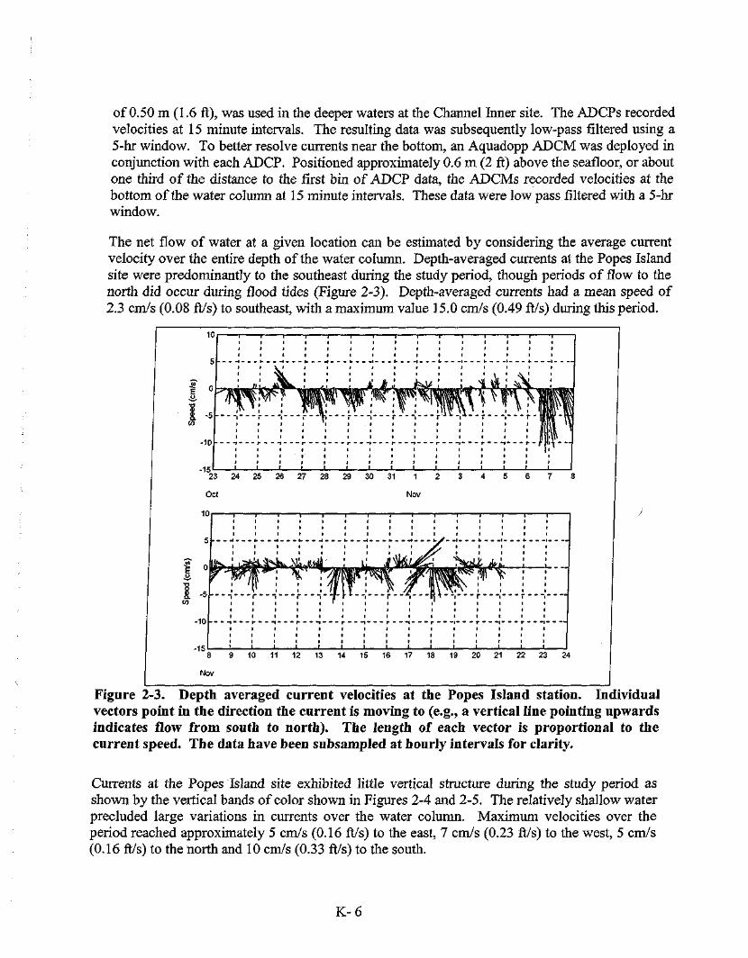
The net flow of water at a given location can be estimated by considering the average current velocity over the entire depth of the water column. Depth-averaged currents at the Popes Island site were predominantly to the southeast during the study period, though periods of flow to the north did occur during flood tides (Figure 2-3). Depth-averaged currents had a mean speed of 2.3 cm/s (0.08 ft/s) to southeast, with a maximum value 15.0 cm/s (0.49 ft/s) during this period.

23 24 25 26 27 28 29 30 31

Oct Nov

20 21 22 23 24

Nov

Figure 2-3. Depth averaged current velocities at the Popes Island station. Individual vectors point in the direction the current is moving to (e.g., a vertical line pointing upwards indicates flow from south to north). The length of each vector is proportional to the current speed. The data have been subsampled at hourly intervals for clarity.

Currents at the Popes Island site exhibited little vertical structure during the study period as shown by the vertical bands of color shown in Figures 2-4 and 2-5. The relatively shallow water precluded large variations in currents over the water column. Maximum velocities over the period reached approximately 5 cm/s (0.16 ft/s) to the east, 7 cm/s (0.23 ft/s) to the west, 5 cm/s (0.16 ft/s) to the north and 10 cm/s (0.33 ft/s) to the south.

K-6

East Velocity Component (cm/s)

.? 4

X 3

i 1 r

IT: I

« '. 1 23

Oct

_I_ _1_ J_ _ l _ _l_ _ l _ 24 25 26 27 28 29 30 31 1

Nov

North Velocity Component (cm/s)

Figure 2-4. Vertical structure of east (top) and north (bottom) components of current velocity at the Popes Island station for the period from 23 October through 8 November 2002.

K-7

1 4

CT

E 4

8 Nov

East Velocity Component (cm/s)

T T T

8

Nov

6

_L. _1_ _1_ _1_ _1_ 10 11 12 13 14 15 16 17 18 19 20 21 22 23 24

North Velocity Component (cm/s)

T T

_l_ _1_ _!_ _l_ _1_ 10 11 12 13 14 15 16 17 18 19 20 21 22 23 .24

Figure 2-5. Vertical structure of east (top) and north (bottom) components of current velocity at the Popes Island station for the period from 8-24 November 2002.

Currents near the bottom of the water column at Popes Island differed little from those observed in the rest of the water column. A comparison of the currents observed by the ADCM to the deepest currents observed by the ADCP reveals only small differences (Figures 2-6 and 2-7). The average current speed recorded by the ADCM during this period was 2.2 cm/s (0.072 ft/s), with a maximum value of 8.3 cm/s (0.27 ft/s). The average speed for the deepest current measured by the ADCP was 2.3 cm/s (0.75 ft/s), while the maximum was 10.4 cm/s (0.34 ft/s).

K-8

1b

10

ADCP ADCM _ 10

ADCP ADCM _

5

0

-5

5

0

-5

tJU \A iu^ eJ^fi ,-&&* sA \j&h \JhJ! w kk 5

0

-5

/ * fcA w\u p *V* ^™ W ^

P m fir ^ TO

ir ̂ AT

5

0

-5 \l

* 23 24 25 26 27 28 29 30 31 1 2 3 4 5 6 7 8

Oct Nov

1 5 l — I — I — I — I — I — I — I — I — I — I — I — I — I — I — I — I ADCP

1 0 . ADCM .

S— oik A A A Ah*. ^y&^&tLJ^h^LM'ldArA |f™Mff|W ftfv^'i

J 1 I I 10 11 12 13 14 15 16 17 18 19 20 21 22 23

Nov

Figure 2-6. A comparison of the eastward component of near bottom current velocity as measured by the ADCP (blue) and the ADCM (red) at the Popes Island station.

23 24 25 26 27 28 29 30 31

Oct

15 — ADCP — ADCM _

it E

•a =

loci

ty

A/1 kt A/ $U yf W\l ̂4 J M A/ fill U-iL*j£i 14 f i L_

ard

Ve

n c

JV FY pry nrwi p 1 1 / !?/ ff wy/| /M VI NA | l>

*lorth

v\

3 C

V

. 1 * 9 10 11 12 13 14 15 16 17 19 20 21 22 23 24

Nov

Figure 2-7. A comparison of the northward component of near bottom current velocity as measured by the ADCP (blue) and the ADCM (red) at the Popes Island station.

K-9

At the Channel Inner site, depth-averaged currents showed a regular variation in response to the tides (Figure 2-8). Flow to the south during ebb tide appeared slightly stronger and more sustained than the northward flow observed during flood tide. Depth-averaged currents averaged 4.0 cm/s (0.13 ft/s), with a maximum value 16.3 cm/s (0.53 ft/s) during the study period.

Nov

Figure 2-8. Depth averaged current velocities at the Channel Inner station. Individual vectors point in the direction the current is moving to (e.g., a vertical line pointing upwards indicates flow from south to north). The length of each vector is proportional to the current speed. The data have been subsampled at hourly intervals for clarity.

Horizontal currents at the Channel Inner site exhibited substantial vertical structure over the course of the study period (Figures 2-9 and 2-10). This is particularly evident in the north velocity component. At the surface, flow tends toward the south, particularly during ebb tide, while at the same time flow at depth is predominantly toward the north.

K-10

1Dr ^ i i

East Velocity Component (cm/s) ~ T 1 — • — i — * — i 1 1 1 i r 1 r ~

I i I

iJf I 1 I « 1 If 11 23 24 25 26 27 28 29 30 31 1 2 3 4 5 6 7 8 Oct Nov

North Velocity Component (cm/s)

Figure 2-9. Vertical structure of east (top) and north (bottom) components of current velocity at the Channel Inner station for the period from 23 October through 8 November 2002

East Velocity Component (cm/s)

5 , '

, *

t i ' i _ j / i i 3

/ill! i l l

' » ' ' ' i ' i r I 9 10 11 12 13 14 15 16 17 18 19 20 . 21 22 23 24

North Velocity Component (cm/s)

11

Figure 2-10. Vertical structure of east (top) and north (bottom) components of current velocity at the Channel Inner station for the period from 8-24 November 2002.

A comparison of the currents observed by the ADCM to the deepest currents observed by the ADCP shows the most significant difference to be a slight decrease in current speed near the bottom (Figures 2-11 and 2-12). The average current speed recorded by the ADCM during this period was 3.0 cm/s (0.098 ft/s), with a maximum value of 11.0 cm/s (0.36 ft/s). The average speed for the deepest current measured by the ADCP is 4.0 cm/s (0.13 ft/s), while the maximum was 15.2 cm/s (0.50 ft/s)

20 ADCP ADCM

-52 -m

ocity

(cm

L y Ah? *\, ffr HH \t% -ftyi htk A/1 «to h A§ M .M d ^ m ff fV pi ̂ rfr jm iW1 Afy (n w f'W ity \i

TO " 1 U

111

.onl 8 9 10 11 12 13 14 15 16 17 18 19 20 21 22 23 24

Nov

Figure 2-11. A comparison of the eastward component of near bottom current velocity as measured by the ADCP (blue) and the ADCM (red) at the Channel Inner station.

K-12

Nov

9 10 11 12 13 14 15 16 17 18 19 20 21 22 23 24

Figure 2-12. A comparison of the northward component of near bottom current velocity as measured by the ADCP (blue) and the ADCM (red) at the Channel Inner station.

2.3 Total Suspended Sediments

Optical backscatter was measured continuously at each of the three long-term deployment stations using D+A Optical Backscatter Sensors (OBSs). At the Popes Island and Channel Inner stations the OBSs were part of the ADCM instrument package, while at the Tide Gauge station it was a separate instrument. Optical backscatter was measured at 15 minute intervals at all three locations. Measurements of optical backscatter were generally low, averaging 2.7 (Nephelometric Turbidity Units (NTU) at Popes Island, 9.1 NTU at Channel Inner and 4.3 NTU at the Tide Gauge station. Deviations from these values were typically sudden spikes to extremely high values, with optical backscatter measurements reaching values of as much as 291.6 NTU (Popes Island), 448.0 (Channel Inner) and 210.0 (Tide Gauge). These excursions were short lived, lasting a few hours at most, except for one event lasting almost a day at Channel Inner. The Channel Inner station also experienced significantly larger and more frequent events than either the Popes Island or the Tide Gauge station.

K-13

50C Popes Island Channel Inner

S" 300 S" 300 S" 300

1 CO

g 200 J CO

g 200

100

0 2

| 100

0 2

. i . . . . l j * 1 . II

100

0 2 3 24 25 26 27 28 29 30 31 1 2 3 4 5 6 7 8

Oct Nov

500 Popes Island

400

3" 300

—— Channel Inner 400

3" 300

Tide Gauge 400

3" 300

400

3" 300

g 200 - 1 g 200 -

w a

I „L lL_l L_ .„ 1 , J 1 .1 * t e . Ml J

8 9 10 11 12 13 14 15 16 17 18 19 20 21 22 23 24

Nov

Figure 2-13. Optical backscatter measured at the Popes Island (blue), Channel Inner (red) and Tide Gauge (black) stations during the study period.

In order to relate optical backscatter to sediment levels in the water column, measurements of total suspended sediment (TSS) concentrations were made at the three station locations on five occasions during the study period (Table 2-2). Multiple samples were taken at a height of approximately 1 m (3.3 ft) above the seafloor on each occasion. Mean values of the three samples of TSS are compared to OBS measurements at the corresponding site at the same time in Figure 2-14.

Table 2-2. Total suspended sediment sampling schedule. Standard Time (LST).

Times are given as Local

Date Site 23 Oct INov 7 Nov 14 Nov 22 Nov Popes Island 9:50 8:58 13:50 8:50 11:30 Channel Inner 11:50 9:15 13:00 9:10 9:38 Tide Gauge 11:00 9:30 15:00 9:30 8:50

K-14

6 •

i i i i i i 1 1 j

• Popes Island B Channel Inner + Tide Gauge 6

1 1 j

• Popes Island B Channel Inner + Tide Gauge

5

=^ A

BS (

NTl

O "

2

1

n

• BH ,

O "

2

1

n

"•""""I

- - • • - ! • i i n !

m

O "

2

1

n

"•""""I

- - • • - ! • i i n !

m

>

10 20 30 40 50 TSS (mg/L)

60 70 80 90

igure 2-14. Optical backscatter plotted against total suspended sediment for the Popes Island (blue), Channel Inner (red) and Tide Gauge (black) stations.

2.4 Chemistry

Elutriate tests are performed to estimate the release of soluble contaminants during dredging operations. A combination of 20 sediment and 80% site water is mixed and allowed to settle. The liquid is then analyzed for contaminant concentrations. The protocol was designed to mimic the initial concentration levels when sediments are released in the water column (Averett, 1989). Elutriate analyses were performed on samples from six stations within Inner New Bedford Harbor to determine background pollutant levels (Table 2-3 and Figure 2-1) and reported in SAIC (2002). Aluminum, copper, nickel, silver and Total PCBs registered above the chronic exposure levels established by the United States Environmental Protection Agency (EPA) at all sites for which analyses were performed. Lead exceeded chronic exposure levels at the NBH-202 station, Benzo(b)fluoranthene exceeded chronic exposure levels at the NBH-202 and NBH-207 stations, and Benzo(k)fluoranthene exceeded chronic exposure levels at NBH-202, NBH-205, NBH-206 and NBH-207. In addition, acute exposure levels were exceeded for aluminum at NBH-202 and NBH-207, and for copper at NBH-201, NBH-202, NBH-205, NBH-206 and NBH-207. Stations NBH-202, a CAD Channel Inner site, and NBH-207, the Fish Island site, showed generally higher concentrations than the other sites.

K-15

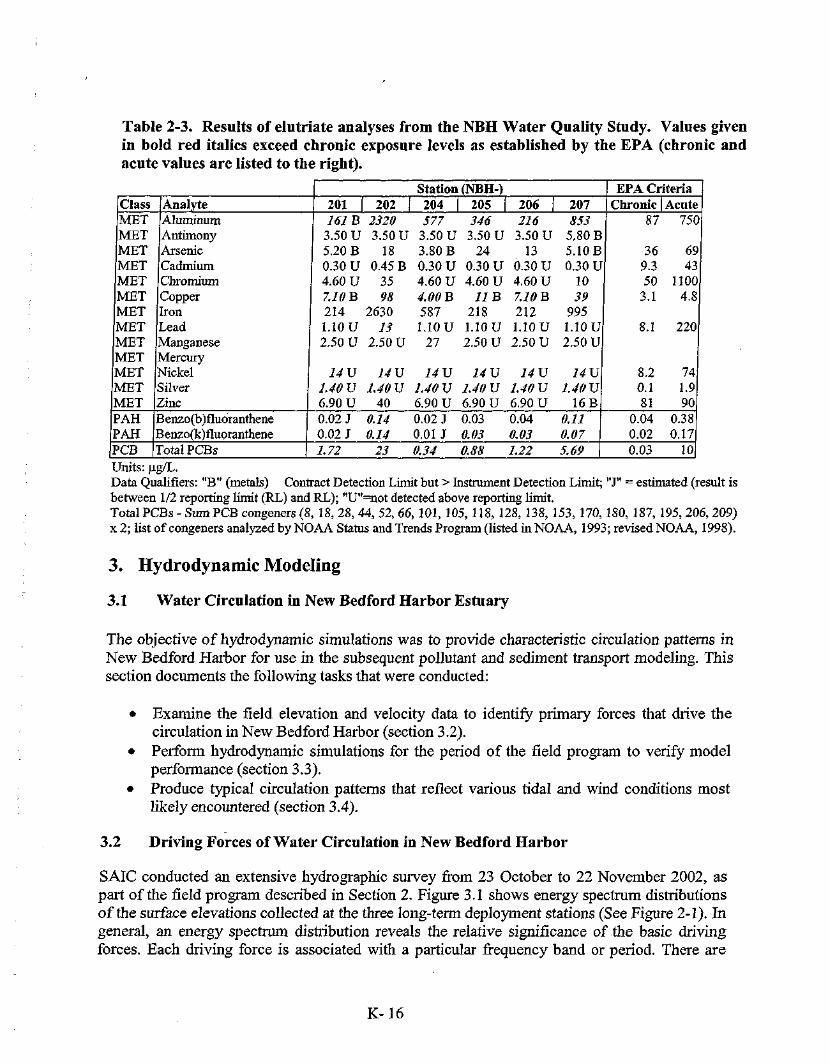
Table 2-3. Results of elutriate analyses from the NBH Water Quality Study. Values given in bold red italics exceed chronic exposure levels as established by the EPA (chronic and acute values are listed to the right).

Station (NBH-) EPA Criteria Class Analyte 201 202 204 205 206 207 Chronic Acute MET Aluminum 161 B 2320 577 346 216 853 87 750 MET Antimony 3.50 U 3.50 U 3.50 U 3.50 U 3.50 U 5,80 B MET Arsenic 5.20 B 18 3.80 B 24 13 5.10 B 36 69 MET Cadmium 0.30 U 0.45 B 0.30 U 0.30 U 0.30 U 0.30 U 9.3 43 MET Chromium 4.60 U 35 4.60 U 4.60 U 4.60 U 10 50 1100 MET Copper 7.10 B 98 4.00 B 11 B 7.10 B 39 3.1 4.8 MET Iron 214 2630 587 218 212 995 MET Lead 1.10U 13 1.10U 1.10U 1.10U 1.10U 8.1 220 MET Manganese 2.50 U 2.50 U 27 2.50 U 2.50 U 2.50 U MET Mercury MET Nickel 14 U 14 V 14 V 14 V 14 V 14 V 8.2 74 MET Silver 1.40 V 1.40 V 1.40 V 1.40 V 1.40 V 1.40 V 0.1 1.9 MET Zinc 6.90 U 40 6.90 U 6.90 U 6.90 U 16B 81 90 PAH Benzo(b)fluoranthene 0.02 J 0.14 0.02 J 0.03 0.04 0.11 0.04 0.38 PAH 3enzo(k)flupranthene 0.02 J 0.14 0.01 J 0.03 0.03 0.07 0.02 0.17 PCB Total PCBs 1.72 23 0.34 0.88 1.22 5.69 0.03 10 Units: ug/L. Data Qu alifiers: "B" (metals) Contract Detection Limit but > Instrument Detection Limit; "J" = estimated (result is between 1/2 reporting limit (RL) and RL); "U"=not detected above reporting limit. Total PCBs-Sum PCB congeners (8, 18,28,44,52,66, 101, 105, 118, 128, 138, 153, 170, 180, 187, 195,206,209) x 2 ; list of congeners analyzed by NOAA Status and Trends Program (listed in NOAA, 1993; revised NOAA, 1998).

3. Hydrodynamic Modeling

3.1 Water Circulation in New Bedford Harbor Estuary

The objective of hydrodynamic simulations was to provide characteristic circulation patterns in New Bedford Harbor for use in the subsequent pollutant and sediment transport modeling. This section documents the following tasks that were conducted:

• Examine the field elevation and velocity data to identify primary forces that drive the circulation in New Bedford Harbor (section 3.2).

• Perform hydrodynamic simulations for the period of the field program to verify model performance (section 3.3).

• Produce typical circulation patterns that reflect various tidal and wind conditions most likely encountered (section 3.4).

3.2 Driving Forces of Water Circulation in New Bedford Harbor

SAIC conducted an extensive hydrographic survey from 23 October to 22 November 2002, as part of the field program described in Section 2. Figure 3.1 shows energy spectrum distributions of the surface elevations collected at the three long-term deployment stations (See Figure 2-1). In general, an energy spectrum distribution reveals the relative significance of the basic driving forces. Each driving force is associated with a particular frequency band or period. There are

K-16

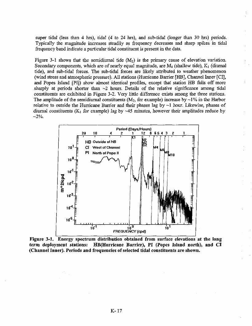
super tidal (less than 4 hrs), tidal (4 to 24 hrs), and sub-tidal (longer than 30 hrs) periods. Typically the magnitude increases steadily as frequency decreases and sharp spikes in tidal frequency band indicate a particular tidal constituent is present in the data.

Figure 3-1 shows that the semidiurnal tide (M2) is the primary cause of elevation variation. Secondary components, which are of nearly equal magnitude, are M4 (shallow tide), Ki (diurnal tide), and sub-tidal forces. The sub-tidal forces are likely attributed to weather phenomenon (wind stress and atmospheric pressure). All stations (Hurricane Barrier [HB], Channel Inner [CI], and Popes Island [PI]) show almost identical profiles, except that station HB falls off more sharply at periods shorter than ~2 hours. Details of the relative significance among tidal constituents are exhibited in Figure 3-2. Very little difference exists among the three stations. The amplitude of the semidiurnal constituents (M2, for example) increase by - 1 % in the Harbor relative to outside the Hurricane Barrier and their phases lag by ~1 hour. Likewise, phases of diurnal constituents (Ki for example) lag by ~45 minutes, however their amplitudes reduce by -2%.

20 10 Period (Days/Hours)

4 2 1 12 8 6 5 4 3 2

1 0 1 4 -

,0

~i 1 1 r

H B Outside of HB

CI West of Channel

PI North of Pope II

FREQUENCY (cpd)

Figure 3-1. Energy spectrum distribution obtained from surface elevations at the long term deployment stations: HB(Hurricane Barrier), PI (Popes Island north), and CI (Channel Inner). Periods and frequencies of selected tidal constituents are shown.

K-17

xm?mm^^&

Figure 3-2. Tidal harmonic constituents obtained from surface elevations at the long term deployment stations (positioned in order from south (Hurricane Barrier) to north (Popes Island).

Similar observations can be made for the currents measured at the Channel Inner and Popes Island stations. No current meter was deployed at the Hurricane Barrier station. Figure 3-3 shows the energy spectrum distributions obtained from the vertically averaged velocities. The trend is similar to the one for elevations; with a falloff at higher frequencies and the existence of tidal frequency spikes. The energy in sub-tidal spectrums, however, becomes more prominent at the shallower station, Popes Island with a MLW depth of 2.6 m (8.5 ft) compared to 9.2 m (30 ft) at Channel Inner. Magnitudes of energy at the sub-tidal periods (~2 to 4 days) equal the tidal (M2) components. Also noticeable is the difference at sub-tidal periods in the east/west versus south/north components. This difference indicates wind forces have significant influence on currents.

K-18

20 10 1 1 r

CI>Average:East/West

Period (Days/Hours) A 2 1 12 8 6 5 4 3 2

1 1 — n — i — i —

Figure 3-3. Energy spectrum distributions obtained from vertically averaged velocities at the long term deployment stations, Channel Inner (CI) and Popes Island (PI).

There are some differences in elevation versus velocity spectrum distributions, however, due to the inherent differences in these hydrodynamic quantities. Elevations are integrated quantities over the water depth and the region. Velocities are highly variable and dependent on depth of observation and immediate local morphology. This is why the elevation spectrum distributions look very similar for all stations while the velocity spectrum distributions look different.

The elevation and velocity spectrum distributions reveal that tides and winds are the primary causes that drive circulation in the region. This observation can also be inferred by examining the variations of elevation and velocity in time. Figure 3-4 shows observed winds (New Bedford municipal airport), elevation (outside of the Hurricane Barrier) and velocities (Channel Inner and Popes Island North) together on the same time axis. All forces drive the circulation with their own frequencies or random times: half daily tidal cycles, spring-neap fortnightly cycles and episodic wind events. Although the variation of velocities is very complex, the response to wind is particularly noticeable through time. Velocities in Figure 3-4 are shown for surface, vertically averaged, and bottom. At the Channel Inner station, with a 9.2 m (30 ft) water depth, the surface and bottom velocities are quite different. The surface velocities are larger, more variable, and generally flow to the south, while bottom velocities are smaller and show an oscillating north-

K-19

south direction. Velocities at Popes Island North, with a 2.6 m (8.5 ft) water depth, are more uniform vertically with somewhat higher speeds t the surface than at the bottom.

Wind Observed (New Bedford Airport)

Elevation (Out side of Harri airier)

Surface Velocity (West side off Channel)

Oct 22 Novl

m/s

m -\ 1 0.5 0

-0.5 -1

Figure 3-4. Time series stack plot of observed wind, elevation and velocity data.

K-20

In general, typical driving forces in normal estuarine circulation are tide, wind, and density gradient. Tide and wind influence are clearly seen in the observations. The significance of the density gradient is based on freshwater inflows. If the amount of freshwater inflow is small relative to the estuary size, the density gradient is not expected to play a significant role. The evidence of density gradients can be seen in the longitudinal salinity. No salinity observation were made for the period of field investigation but other studies concluded the density driven flow would be much less than 1 cm/s (see the discussion in Abdelrhman [2002]) south of Coggeshall St./I-95 Bridge, the lower portion of the Inner Harbor where the dredging and disposal operations are planned.

3.3 Hydrodynamic Model Application

3.3.1 Description of Hydrodynamic Model WQMAP/BFHYDRO

ASA has developed and applied evolving versions of sophisticated model systems (Swanson 1986, Spaulding et al., 1999) for use in studies of coastal waters for more than two decades. WQMAP, as the model system is known, uses a three dimensional boundary fitted finite difference hydrodynamic model (BFHYDRO) developed by Muin and Spaulding (1997a and b). The model has undergone extensive testing against analytical solutions and used for numerous water quality studies. Some applications particular to dredging studies in the northeastern United States are

• Water quality impacts of dredging and disposal operations in Boston Harbor (Swanson and Mendelsohn 1996)

• Dredged material plume for the Providence River and Harbor Maintenance Dredging Project (Swanson et al., 2000)

• Simulations of sediment deposition from jet plow operations in New Haven Harbor (Swanson et al., 2001)

• Simulations of sediment transport and deposition from jet plow and excavation operations in the Hudson River (Galagan et al., 2001)

The grid system used in the boundary-fitted coordinate model system is unique in that grid cells can be aligned to shorelines and bathymetric features (like dredged channels) to best characterize the study area. In addition, grid resolution can be refined to obtain more detail in areas of concern. This gridding flexibility is critical in representing the New Bedford Harbor waters where geometry is highly variable and complex.

3.3.2 New Bedford Harbor Grid

The domain of the hydrodynamic model for this application included the entire New Bedford Harbor, Inner and Outer, and a portion of Buzzards Bay. Figure 3-5 shows the large variation of cell size. The Buzzards Bay portion served as the open boundary condition where a cell size of -700 m (2300 ft) was employed. The finest grid resolution of ~50 m (165 ft) was located in the

K-21

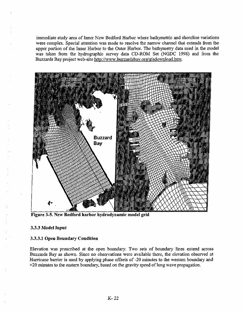
immediate study area of Inner New Bedford Harbor where bathymetric and shoreline variations were complex. Special attention was made to resolve the narrow channel that extends from the upper portion of the Inner Harbor to the Outer Harbor. The bathymetry data used in the model was taken from the hydrographic survey data CD-ROM Set (NGDC 1998) and from the Buzzards Bay project web-site http://www.buzzardsbay.org/gisdownload.htm.

Figure 3-5. New Bedford harbor hydrodynamic model grid

3.3.3 Model Input

3.3.3.1 Open Boundary Condition

Elevation was prescribed at the open boundary. Two sets of boundary lines extend across Buzzards Bay as shown. Since no observations were available there, the elevation observed at Hurricane barrier is used by applying phase offsets of -20 minutes to the western boundary and +20 minutes to the eastern boundary, based on the gravity speed of long wave propagation.

K-22

3.3.3.2 Surface Wind Stress

Two wind data sets from New Bedford Municipal Airport (-5.3 km [3.3 mi] north-west of Popes Island) and Buzzards Bay NOAA Buoy (-29 km [18 mi] south-south-west of Popes Island) were considered. During the period of the field program, their directions were nearly identical but speeds at the buoy were substantially larger. Although the NOAA Buzzards Bay Buoy provided a better estimate of the unobstructed wind, the wind record from the airport was selected because of its proximity to the Inner Harbor.

3.3.3.3 Other Model Parameters

The computational time step defined how often the model calculated velocities and was chosen to be 300 sec, the largest allowed without causing model instabilities. The number of vertical layer was chosen as 7, sufficient to resolve the vertical structure of the horizontal currents. The bottom stress coefficient, based on Manning's equation was selected as 0.03, typical for estuaries. The wind stress coefficient was selected as 0.0014. The depth dependent vertical viscosity was chosen as 0.0005 + 0.0001 times the local depth (m) and expressed in m2/sec.

3.3.4 Simulation Results

The hydrodynamic model simulated the circulation from 20 October to 20 November 2002, the period of the field program, with aforementioned model inputs and parameters. Figure 3.6 shows comparisons of observed versus simulated elevations at the three field stations. The station outside of Hurricane Barrier shows the best match. This is not surprising since the open boundaries were based on this elevation (+/- 20 min phase offset but the same amplitude). There was very little elevation gradient between Buzzards Bay and the Outer Harbor. Simulated elevations at Channel Inner and Popes Island are in good agreement in amplitude but their phases slightly lead the observations.

Figure 3-7 and 3-8 show comparisons of the observed versus simulated velocities at the Channel Inner and Popes Island North stations, respectively. Magnitudes of the velocities agreed well with the observations. The flow directions, however, differed in various degrees during the simulation period. The apparent complexity is due to wind stress. During some periods, the currents strongly correlated with the wind. For example, during the period (Oct 24 - Oct 30), wind blew steadily from the NNW direction. The observed surface currents flowed to the SSE, showing a strong positive wind/current correlation. On other occasions, i.e., from Nov 8 to Nov 12, strong winds blew from the SW~SSW direction but both observed surface currents appeared unaffected. The simulated current showed a contrary response during these periods: weak flow in the first period and strong flow to the later period, although the surface currents were always positively correlated with the wind. This suggests actual winds on the water may be different from the wind observed at the airport. However, simulations using rotated winds were tried but with no significant improvement.

K-23

F Elevation: Outside of Hurricane Barrier

kd^^MM w fW^rmmn^fj k

r- ?l

i l l

nriBter

AA.̂ .-fl A AAAjf/UAA AA Afl f t /W

1.5

1

0.5 ,

0

-D.5

-1 •

-1.5,

- t 1-5

p

Nov1 Nov 8 Nov 15

Figure 3-6. Comparisons of elevations: observed (thick blue line) versus simulated (thin red line).

In conclusion, the simulated elevations and velocity magnitudes agree very well with the observations. This assures overall hydrodynamics are consistent. The difference in the flow direction can be attributed to the uncertainty of the actual forcing wind magnitude.

K-24

'. figure 3-7. Comparison of observed versus simulated velocity at Channel Inner station

K-25

Wind Observed (New Bedford Airport)

jjAjpj ]**^^'yjpy

Surface Velocity (Observed at North of Popes Island)

(Simulated)

J*ft\yW ^^<fr"fo^fy^

Vertically Averaged (Observed)

Bottom (Observed)

(Simulated)

Nov1

- I

w - -1

r (Simulated)

Nov 8 Nov 15

Figure 3-8. Comparison of observed versus simulated velocity at Popes Island north station.

K-26

3.4 Characteristic Circulation Scenarios

The analysis of the field observations and hydrodynamic simulations confirmed that the major forces driving the circulation in New Bedford Harbor are astronomic tides and winds. Since the purpose of the mass transport simulations was to predict the distribution of dredged pollutants and sediments under typical wind and tidal conditions, the particular periods (season or date) of such simulations were not determined a priori. The approach taken here was to develop a set of circulation scenarios that reflected most likely conditions. These scenarios were comprised of various tidal conditions and most probable wind conditions. Tidal variations considered were spring, mean and neap tides. Unlike the astronomic tide, which is predictable, wind is very episodic and must be approached in a statistical sense.

3.4.1 Wind Climate for Inner New Bedford Harbor

The variability of the wind at the New Bedford Municipal Airport was examined. Figure 3.9 and Table 3.1 shows the seasonal probability of wind direction in 30° increments. Two prominent wind directions found were south-west-south (SWS) and north-west-west (NWW). Nearly 50% of the time wind blew from the SWS direction in summer and the NWW direction in winter. This tendency remained to a lesser degree during spring and autumn. The probability that wind speed was less than 3.0 m/s (6.7 mph), considered as calm wind, is ~10.7% on average.

Table 3.1. Variations of winds at New Bedford Municipal Airport by season.

Chance wind blows from Calm wind either SWS or NWW (<3.0 m/s)

Winter 45.5% 8.4 % Spring 35.4 11.1

Summer 50.9 13.8 Autumn 35.3 10.1

Wind speed was quite variable during the seasons. The average wind speed for both directions (excluding the calm wind period) was calculated to be 8.2 m/s (18.3 mph), equivalent to a wind stress of approximately 1 dyne/cm2 (0.0021 lbs/ft2).

3.4.2 Circulation Scenarios

Three tidal conditions (neap, mean, and spring) and three wind conditions (calm, SWS, NWW at 8.2 m/s speed) were combined to make the nine circulation scenarios summarized in Table 3.2.

K-27

Figure 3-9. Probability of wind direction of the four seasons.

Table 3.2. Circulation scenarios based on tide and wind conditions.

Circulation Scenario 1 2 3 4 5 6 7 8 9

Tide Range Wind

Neap (0.7 m [2.3 ft]) Mean (1.0 m [3.3 ft]) Spring (1.4 m [4.6 ft]) Neap (0.7 m [2.3 ft]) Mean (1.0 m [3.3 ft]) Spring (1.4 m [4.6 ft]) Neap (0.7 m [2.3 ft]) Mean (1.0 m [3.3 ft]) Spring (1.4 m [4.6 ft])

Calm calm calm SWS8.2m/s SWS 8.2 m/s SWS 8.2 m/s NWW 8.2 m/s NWW 8.2 m/s NWW 8.2 m/s

To assess the direct effect of tidal conditions and winds, hydrodynamic simulations were run separately for each component. Figures 3-10 and 3-11 show simulated surface flood speed contours and velocity vectors for neap, mean and spring tides under calm wind conditions, respectively. As the tide range doubles from neap to spring conditions, the velocity also approximately doubles throughout the region. Figures 3-12 and 3-13 show simulated surface and bottom flood speed contours and velocity vectors driven by the SWS wind and mean tide, respectively. There is a strong surface flow heading downwind but modulated by the Inner Harbor geometry. The bottom flow is much lower in magnitude. Figures 3-14 and 3-15 show simulation results driven by the NWW wind and mean tide. Here the surface flow is again downwind with a significant upwind flow along the bottom in the channel. In general, surface and shallow waters tend to move with the wind while flows in deeper areas adjust by compensating the flow to balance the direct wind-induced flows.

K-28

Nine hydrodynamic simulations using the combination of tide and wind conditions were then executed. Table 3.3 compares the simulated speed (vertically averaged) at the two field stations. The result indicates flows driven only by tides are very weak, varying from 1.4 to 4.3 cm/s (0.046 to 0.14 ft/s). Wind substantially increases flow velocities, the SWS wind generating a range of speeds between 5.1 and 9.6 cm/s (0.17 to 0.32 ft/s) and the NWW wind generating a range of speeds between 6.5 and 15.7 cm/s (0.21 to 0.52 ft/s).

Table 3.3 Vertically averaged simulated speed at two field station locations for the nine circulation scenarios.

\ 1

1 Circulation Scenario 1 Channel Inner Popes Island North Tide Wind Speed (cm/s) Speed (cm/s) Neap Calm 2.1 1.4 Mean Calm 3.0 1.9 Spring Calm 4.3 2.6 Neap SWS @ 8.2 m/s 5.1 9.6 Mean SWS @ 8.2 m/s 6.0 9.3 Spring SWS @ 8.2 m/s 7.1 9.4 Neap NWW @ 8.2 m/s 13.6 6.5 Mean NWW @ 8.2 m/s 14.6 7.0 Spring 1 NWW @ 8.2 m/s 15.7 1 7.5 1

i i

t /

if x.1

(m/s)

j

.i> 1 1 1 i > I :

i 1 ?"

•iA-> 1G r "

l

i 1 ?"

1 I

! 1

Figure 3-10. Surface flood speed contours for neap, mean and spring (from left to right) tide conditions under calm wind conditions.

K-29

Figure 3-11. Surface flood velocity vectors for neap, normal, and spring (from left to right) tidal conditions under calm wind conditions.

«*

••.2 m/s

I \ .

\''„ * - * v

t '>-

*"*V w * s \ .

V

v.

x:. Gprud (m/s)

:-> .02 ' - " '

02-> .01 ftjj?

04 -> .06 1 P 3

06-> .08

08-> .1

.:-> .12

12-> .14

.:4-> .16

i6-> .18

13-> .2

> .2

=- I

%

Figure 3-12. Surface (left) and bottom (right) speed contours for SWS wind.

K-30

XI '

i'

m/;,

i

A|>|ily

i'

-. m/;,

i

i'

-. m/;,

i

• L H i' > - .rs

i.--,,:, |L0 ,, 7 i

it n?m/s

» .-•<".,

*«r i."?;-jS-:'-%.V -A - •

. - ' . -

Figure 3-13. Surface (left) and bottom (right) velocity vectors for SWS wind.

\ II ? m/r.

\ -:.

\ : . T . . V - .

Speed

(m/s)

0-> .02 ' '"

02-> .04 ;%j j |

06-> .08 p H

OB->. I | ;

1 -> .12 *

> 2 • •

x »

• — i*ii in tn«tnimiiB

Figure 3-14. Surface (left) and bottom (right) speed contours for NWW wind.

K-31

Figure 3-15. Surface (left) and bottom (right) velocity vectors for NWW wind.

The set of scenarios listed in Table 3.3 were rerun with bathymetry that reflects the proposed Popes Island CAD cell excavation, from 2.6 to 17 m (8.5 to 56 ft), to simulate the circulation for dredge material disposal simulations into the cells. The results of these additional hydrodynamic runs were very similar to the present bathymetry runs. Velocities for tide only cases simply showed a reduction in speed (Figure 3-16). The immediate vicinity of the CAD site, however, showed surface water moving in direct response to wind and a reverse flow developed at the bottom for wind driven cases (Figures 3-17 and 3-18).

K-32

Figure 3-16 Comparison of flood surface velocity vectors for spring tide and calm winds: existing (left) versus excavated (right) bathymetry. Red polygons represent cells in the proposed CAD facility at north of Popes Island.

Figure 3-17 Comparison of velocity vectors at surface (left panels) and bottom (right panels) for the NWW wind case, existing (upper panels) versus excavated (lower panels) bathymetry. Red polygons represent cells in the CAD facility at north of Popes Island.

K-33

Figure 3-18 Comparison of velocity vectors at surface (left panels) and bottom (right panels) for the SWS wind case, existing (upper panels) versus excavated (lower panels) bathymetry. Red polygons represent cells in the CAD facility at north of Popes Island.

K-34

4. Dredged Material Modeling using SSFATE

4.1 Excavation of Popes Island CAD Cell

All of the dredged sediments from the waterways are to be disposed in the PIN-CAD facility. The capacity of the CAD site was designed to accommodate many dredging projects. Six cells are planned at the PIN-CAD site (shown in Figures 3-16 to 3-18). The largest cell volume is 1,739,362 m3 (2,275,000 yd3), and the volume for the small cells ranges from 62,980 m3 (82,375 yd3) to 65,331 m3 (85,459 yd3). Excavation of these CAD cells exceeds the volume from dredging operations from all the waterways projects..

This report section details the analysis of water column TSS concentration increases due to excavation of the PIN-CAD cells. The process of excavation is similar to maintenance dredging; a clamshell bucket (7 yd [5.4 m ]) is lowered to the bottom (~15 m [50 ft]), grabs the sediment, and the bucket is then raised to the surface, where the sediment is dropped into a barge. This cycle repeats every ~90 sec until the total volume is excavated (lasting up to several months). Water column TSS increases occur if some portions of the sediment become waterbome. Most of the sediment release takes place when the bucket contacts the seafioor. Additional sediment escapes from the bucket while the bucket travels up through water column, particularly if the bucket is not well sealed. Total sediment amount released (source strength of TSS) varies depending on the type of bucket (to be discussed in the next section).

This sediment loss during dredging serves as a TSS source to the water column for the entire period of dredging operation. The distribution of water column concentration of TSS away from the immediate site of operation is governed by how the sediment is transported, settled, and dispersed by ambient currents, in addition to the initial source strength. These processes were simulated by ASA's SSFATE (Suspended Sediment Fate) model.

SSFATE was jointly developed by ASA and the U.S. Army Corps of Engineers (USACE) Engineer Research and Development Center (ERDC). SSFATE is to be one of a family of USACE models that simulate various dredging related activities (e.g., STFATE, dredged material disposal; MDFATE, multiple dump disposals; and LTFATE, long-term mound stability). It has been documented in a series of USACE Dredging Operations and Environmental Research (DOER) Program technical notes (Johnson et al., 2000 and Swanson et al., 2000).

4.1.1 Source Strength Estimation

Dredging operations using a clamshell bucket inevitably disturb the bottom sediments and cause a portion to suspend above the bottom. Sediment losses from the bucket occur during travel through the water column and as the bucket breaks the water surface. There can be additional losses if the excess liquid in the scow is allowed to flow overboard. Typical loss rate ranges 1.5 to 4% for various bucket types shown in Table 4.1.

K-35

Table 4.1. Typical loss rates for different bucket types.

Type of bucket Loss (%) Conventional bucket with over flow

Conventional bucket without over flow Environmental bucket

4 2

1.5 From DOER Technical Notes Collection (ERDC TN-DOER-E12)

Newer buckets (environmental buckets) are designed to minimize resuspension and loss by using various measures, for example, better venting, rubber sealed bucket and level cut capability which reduces side collapsing. The use of such buckets is planned for this project so a loss rate of 1.5% was assumed.

Total suspended solids (TSS) source strength used in the model is the defined as the mass rate of sediment injected into the water column. It can be determined using the following parameters,

• Production rate = 214 m3/hr (280 yd3/hr equivalent to a bucket capacity of 7 yd3 and a cycle time of 90 s)

• Solid fraction = 60% (average of 65.7% for NHB-202-3 and 53.4% for NHB-202-6) • Sediment density = 2,600 kg/m3 (162 lb/ft3)

The mean release rate of sediment is then the quadruple product,

(loss rate) x (production rate) x (solid fraction) x (density) = 1.8 kg/s.

4.1.2 Sediment Characteristics Near the CAD Cell Site

One of the major factors that controls TSS concentration is how fast the sediment settles from the water column back to the bottom. In general, coarser materials have higher settling velocities while the finer materials stay in the water column much longer. By examining size fractions of sediment for the site, basic settling characteristics can be determined. The SSFATE model treats sediments as having five distinct size classes (Johnson, et. Al., 2000),

Table 4.2 SSFATE sediment size classes.

Class Size (micron) Description 1 0 - 7 micron Clay 2 8-35 fine silt 3 36-74 medium fine silt 4 75-130 fine sand 5 >130 coarse sand |

Figure 4-1 shows the distribution of sediment size classes obtained from samples from the proposed PIN-CAD cell site (see Figure 4-2 for locations of the sediment samples). Values of the all sampling stations were averaged (Table 4.3) and used in the SSFATE model.

K-36

Table 4.3 Average sediment size composition of samples from the PIN-CAD site.

Class Description Distribution (%) 1 Clay 25.1 2 find silt 19.0 3 medium fine silt 19.0 4 fine sand 16.5 5 coarse sand 20.5

100%

60%

40%

20%

204 204b 205 206 206(4ft>) 209 210 211 212 213

Popes Island Sediment

Figure 4-1 Sediment type distributions near the PIN-CAD cell site.

K-37

H ®

CAD Cel.s

-> :

E3 • • >

. J

i . -Popes

&' .Island

Figure 4-2 Map showing the PIN-CAD cells and sediment sampling stations.

4.1.3 Predicted TSS Concentrations

SSFATE simulations that represent CAD cell excavations using clamshell bucket dredging were performed for the nine typical hydrodynamic conditions described above. The center coordinate of the largest CAD cell was designated as a representative dredging operation location, which was fixed for the duration of the simulation. TSS concentration distributions due to the clamshell dredging reached a quasi-steady state within two tidal cycles (~1 day). All simulations were run for 3 days.

Presentation of simulation results are shown by:

• Horizontal and vertical views of TSS concentration distribution • Acreage of the area exceeding various concentration levels • Sediment mass balance

Figure 4-3 shows contours of the maximum TSS concentrations throughout the water column over the 3-day simulation period. A vertical section of the concentration distribution was inserted at the base of each plan view. Frames in the figure are organized such that rows display simulations for the three wind conditions and columns for the three different tides.

For the neap only condition (1st row), all TSS distributions appeared to be centered in the dredge site. Overall sediment plume sizes correspond to the tide strength. For the NWW wind cases, all sediment plumes trail to the lee side of the wind direction, whereas the opposite is found for the SWS wind cases. Similar results are obtained for mean and spring tidal conditions, except the size of plume increases with increasing tide range.

K-38

It is important to note that the instantaneous concentrations, which vary widely in time, are significantly smaller than the maximum TSS concentrations presented here.

!~mi(l

1 '' in 1 1 ' i l l m i r l-f> 40 n . 40 •J\ n 'lill m i i 1111 100 tvr J inn M i _ i lain 4(in i J I WO nin H j-sjn > 1 1

a

I !T:

Neap/Calm wind

.• r Mean/Calm wind

X l '

Spring/Calm wind

mq i ^-111 in ./a 111. <il in to Ul III iifi - Ian n m.i xtn C3 ;im « i n mu otjj • • ma- Q

1=3

-~ I

Ik" I : - I

X'- I.

Neap/NWW wind

I -*• .

xii L

Mean/NWW wind

i / • L

i - - .-A ."~^

-— I

Spring/NWW wind

i\, X A~-i i\, ni[i L

•;, - m en X A~-

H I 70 r—i. • '

' va MI C H i \ -. .

H I eu C 3 M I no CZ3 UO 1IKI I 3

»*. V , ' - -i . -- inn sun C D

VMS J11!) C 3 -• _~ •

• ;-4UJ . liilU ^ B

' - • • . - - •

! _ » ? : \ 1 '. "l - - • ; : " : x

I - •

V ,

xi. r

r--

-iii^J.

J I

i.->i

::-.'-!' Neap/SWS wind Mean/SWS wind Spring/SWS wind

Figure 4.3 Maximum TSS concentrations for the nine circulation scenarios. Inserted in each plan view is a vertical section view along the dashed line.

K-39

Figures 4-4 through 4-6 shows the area coverage (acres) exceeding fixed TSS concentration levels in the same order as Figure 4-3. This is essentially the same information as contained in Figure 4-3, except it more direct area comparisons in a quantitative manner. Neap tide also results in smaller areas and spring tide results in larger areas than the mean tide. The analysis presented here did not include the ambient or background TSS concentrations which were sampled during the field program and typically ranged from 3 to 10 mg/L.

Figure 4-7 presents the mass of the fine fractions of sediment remaining in the water column after all settling has occurred. When the system reaches a quasi-steady state, the sediment mass introduced by dredging balances the mass that settles out, so the fraction of sediment that remains waterborne becomes constant. This water column sediment fraction is uniquely distributed by overall size and concentration among the hydrodynamic conditions.

For example, the water column sediment fractions in the NWW case and SWS case are ~2% and - 3 % , respectively. This number indicates that the SWS case produces a larger sediment plume and a higher sediment fraction remaining in the water column, compared to the NWW case. This is caused by advection carrying sediments to the deeper waters, in contrast to the NWW case, in which sediments are transported to shallow water where more settlmg take place. In the case of calm wind conditions, the higher tide conditions have the higher water column sediment fraction. The reason is not obvious. However, there are two possible explanations: 1) the smaller tide range tends to form higher sediment concentrations, which in turn enhance the aggregative settling, 2) the lower tide (lower velocity) provides higher deposition probability (sediments can not be deposited if bottom velocity exceeds a certain threshold).

at i_ o at D) a k . at > o

O <s at

90

80

70

60

50

40

30

20

10

0

B Neap Tide ,

B Normal Tide

' • Spring Tide

60 80

TSS (mg/L) 100 200 400

'. 7igure 4-4 Area coverage (acres) of exceeding specified TSS concentration levels for the calm wind (tide only) condition.

K-40

90

.-* 80

o 70 < —' 60 w 50

B Neap Ti.de

m Normal Tide

D Spring Tide

60 80

TSS (mg/L)

Figure 4-5 Area coverage (acres) of exceeding specified TSS concentration levels for the NWW wind case.

B Neap Tide „

H Normal Tide

• Spring Tide

60 80

TSS (mg/L)

100 200 400

figure 4-6 SWS wind

Area coverage (acres) of exceeding specified TSS concentration levels for the case.

K-41

Q . (0 CI)

ro E C CD E z o z:

Q. CO

Hydrodynamic Conditions

Figure 4-7 Sediment fractions in water column for various hydrodynamic conditions.

4.2 Single Event Disposal into Popes Island CAD Cell

In the previous section, simulations of the TSS increases in the water column due to CAD cell excavation were presented, in which a clamshell bucket operation continuously releases sediments. In this section, TSS concentration increases due to sediment disposal from a scow into the CAD cell is presented. Sediments dredged for channel maintenance and improvement are planned to be stored in a scow as the clamshell bucket removes sediments from the seafloor. When the scow becomes full, it will be moved from the dredging site to a location above the designated CAD cell. Then the scow bottom is opened and the entire contents released. As the sediment descends to the CAD cell floor, some portion of sediment is stripped and remains in the water column. The occurrence of those disposal events is controlled by the clamshell dredging speed of 214 m3/hr (280 yd3/hr) and the scow capacity of 1,530 m3 (2,000 yd3). At this rate, a disposal event will occur every ~12 hours. The approach to simulate TSS concentrations caused by a single scow disposal follows the same procedure employed in the previous section.

4.2.1 Source Strength Estimation due to Scow Disposal Events

Although excavated CAD cells have much deeper water depths (~17 m [ 56 ft]) than the original undisturbed depth (~2.6 m), the time for most of the sediment to reach the bottom is still very short (< 120 sec). This short time span cannot be directly simulated by SSFATE. Instead, the USACE model STFATE (Short-Term Fate dredged material disposal model) was used with

K-42

equivalent input and environmental conditions. STFATE has various operational modes. One option is to simulate convective descent and sediment cloud collapse phase. This output was used to estimate initial source strengths and vertical distribution of waterborne sediment mass.

The estimated portion of the sediment that is stripped during descent has been estimated to be 1% of total sediment in the bucket (ENSR, 2002). Clamshell-dredged, cohesive material has a high proportion of clump content that tends to reach the bottom intact. This stripped loss estimate is comparable to those used in similar projects in Providence and Boston. The vertical distribution of waterborne sediment mass predicted from the STFATE model is given in Table 4.4. Most (85%) of the material immediately falls to the bottom and only 1% remains in the surface less immediately following disposal.

Table 4.4 The vertical distribution of waterborne sediment mass.

Percent of Percent sediment mass

of water column 90 (near surface) 1 70 2 50 4 30 8 10 (near bottom) j 85

4.2.2 Sediment Characteristics of Dredged Materials

Figure 4-8 shows the distribution of sediment classes obtained from the Channel Inner CAD cell site (see Figure 4-9 for locations of the sediment samples). Some of the dredging is expected to take place at this location.. Averaged values of size distributions from these sampling stations were considered to be representative (Table 4.5). The distribution is very similar to the Popes Island one (Table 4.3).

K-43

Table 4.5. Representative sediment size class distribution.

Class Description Distribution % 1 Clay 20.1 2 Fine silt 17.7 3 Medium fine silt 17.7 4 Fine sand 20.1 5 Coarse sand 24.5

Channel Inner Sediment

Figure 4-8 Sediment type distributions near Channel Inner dredging site.

K-44

Figure 4-9. Map showing sediment sampling stations near Channel Inner dredge site.

4.2.3 Model Results for Dredged Material Disposal Operation

SSFATE simulations that represented the fate of the dredged material from disposal operations were performed for the nine hydrodynamic conditions. The bathymetry in which the circulation field was created is substantially deeper (~17 m [50 ft]) at the disposal site than the one used (~2.6 m [8.5 ft]) in the previous PIN-CAD cell excavation simulation. The center coordinate of the largest CAD cell was used as the representative disposal site. Unlike dredging operations, sediment disposal is much quicker. The simulation period was 12 hours.

The simulation results presented in this section include:

• Horizontal and vertical view of TSS distribution • Time series of acreage of exceeding 10 mg/L concentration levels

Figure 4-10 shows a plan view of the maximum predicted TSS concentrations throughout the water column during the 12-hour simulation period. Inserted is a vertical section view of the concentration. The frames in the figure are organized by row (wind conditions) and columns (tide conditions). The rows correspond to calm wind, NWW wind and SWS wind from top to bottom, and the columns correspond to neap, mean, and spring tide from left to right.

All TSS concentration distributions for the tide only scenarios were confined within the PIN-CAD cell since the circulation is too weak (see Figure 3-16) to transport material very far. For the NWW and SWW wind cases, sediment clouds reach the edge of the CAD cells, although most of the sediment remained in the cell. The direction of sediment drift corresponded to the flow guided by a combination of the surface wind stress and the bathymetry of the CAD cell.

K-45

The NWW wind case transported the bottom sediment to the northwest and the SWS wind case transported the sediment to the southwest. It is important to note that the instantaneous concentrations, which varied widely in time, was significantly smaller than the maximum TSS concentrations presented here.

Figure 4-11 shows the area coverage that exceeds a TSS concentration of 10 mg/L (approximately the background threshold) in time. For the case of wind driven circulation, the sediment cloud dissipates within ~ 3 hours. The calm wind tide cases take much longer to settle as most sediment stays in the deep area (~17 m) and so the vertical travel time is increased.

my L | 5 10 • [ >

10 20 • ( 20 40 CZP \ _ _ _ 10 ofl • '

EU Ml C 3 | '„ B0 100 C 3 , ^ ion 7nfl • ' "•

200 400 D l s 400 RIM B l

_ \ooo > C3, j

\ i * -

Neap Calm wind

>-ri ' - i

Mean / C aim wind riifi l

s 10 n in ?fl CZ3 'D ill • 10 BO • LU oil O R0 100 • iiin 700 O " 'OJ 400 •

i mo ttoo • LRiia > O

•a

V 0

S \-

Spriiig^Calni >\ hid

\

,i \ .

1 1 i _- ^ - i | ,'\ V ^ ^ ' X 1 r- 7L X i , 1 r-

i

r~" . r •[! > 1 . 1 r i wn

•- L. -

Neap/NWW wind Mean/NWW wind Spring/NWW wind

K-46

I -

mi; L

s in n ID ta n 20 411 LTi 40 bU LZ: titl 80 • fill 10U I.-I inn ^UG • xua ;ou L i 4011 MUD KB M J B ' 13

\—

X'

I

N-. „ - ' \ 1

in 2<J jr." *»

1 i •

„ r

.. 1.:_-'..:._ 1 : -

- —1

Neap/SWS wind Mean/SWS wind Spring/SWS wind Figure 4-10 Maximum TSS concentrations throughout water column and duration of simulation for the nine hydrodynamic scenarios.

4.00 6.00 8.00 Time (Hours)

10.00 12.00

Figure 4-11. Time series of area coverage (acre) that exceeds TSS concentration of lOmg/L for the nine hydrodynamic scenarios.

5. Pollutant Transport Modeling

5.1 BFMASS Model

The BFMASS model, a component of the WQMAP pollutant transport model system, is a single constituent transport model, which includes first order reaction terms. This model is suitable for

K-47

a single constituent contaminant that is conservative, settles, decays, or grows. This model was used in this application to predict the temporally and spatially varying concentrations associated with transport of equilibrated sediment contaminants (e.g. hydrocarbons and metals) in dissolved phase (i.e. a conservative constituent).

In BFMASS the two- or three-dimensional advection-diffusion equation is solved on the same boundary conforming grid as the hydrodynamic model, BFHYDRO. The model obtains the face-centered, contra-variant velocity vector components from the hydrodynamic model. This procedure eliminates the need for aggregation or spatial interpolation of the flows from the hydrodynamic model and assures mass conservation. The transport model is solved using a simple explicit finite difference technique on the boundary conforming grid (ASA, 1997). The vertical diffusion, however, is represented implicitly to ease the time step restriction caused by the normally small vertical length scale that characterizes many coastal applications. The horizontal diffusion term is solved by a centered-in-space, explicit technique. The solution to the advection-diffusion equation has been validated by comparison to one- and two-dimensional analytic solutions for constant plane and line source loads in a uniform flow field and for a constant step function at the upstream boundary. The model has also been tested for salinity intrusion in a channel (Muin, 1993).

5.2 Model Application

5.2.1 Disposal Operations

Contaminated dredged material will be buried in the confined aquatic disposal (CAD) facility that is proposed north of Popes Island (PIN). There are two types of dredging operations that will use the facility that are classified large and small volume projects. Since the extent or likelihood of large projects are uncertain at this time, pollutant transport and fate simulations were focused on disposal activity for a small project whose volume is on the order of 30,600 m3 (40,000 yd3). Table 5-1 lists the details of a likely disposal activity in addition to the associated dredging operation. These details were developed jointly with Maguire personnel. The use of two split-hull scows were assumed, alternating to carry and dispose dredged material during two 12-hr shifts per day. Dimensions of each barge were 3 m (10 ft) wide by 76 m (250 ft) long with a holding capacity of 1,530 m3 (2,000 yd3).

Table 5-1. Assumed details for dredging and disposal operations in New Bedford Harbor.

Operation Parameter Detail

Dredging Dredging Sites Maneuvering channel, berth,

wharf, inner federal navigation channel

Dredging

Dredging Project Volume 30,600 m (40,000 yd3)

Dredging

Composition of dredged material (%)

Contaminated material

90

Dredging

Types of dredging operation for

Contaminated material

Continuous

Dredging

Dredging equipment used for

Contaminated material

Environmental bucket

K-48

Bucket capacity Environmental bucket

5,4 m" (7 ydJ)

Dredging rate (min/grab) 1.5 Duration of dredging operation (day) 6 Number of concurrent dredging operations

One

Time of dredge operations 1 June 2003 ~ 1 January 2004

Loss rate during dredging operation 1.5%

Disposal

Disposal Site Location Popes Island North

Disposal

Number of scows 2

Disposal

Scow Capacity (yd3) 1,530 mJ (2,000 yd")

Disposal Dimension of scow 3 m (10 ft) wide x 76 m (250

ft) long Disposal Type of scow Split-hull

Disposal

Duration of disposal operation (sec) 5

Disposal

Typical cycle from barge loading to disposal (hour)

12

5.2.2 Source Strength

The source strength is the mass of pollutant entering the system on a rate basis. Three types of source strengths can be specified in BFMASS: 1), an instantaneous release; 2), a constant release over time; and 3), variable release over time. An instantaneous source release is the mass of material released to the water column from an entire split-hull barge load in a second. A constant source is defined as the mean loading to the water column from multiple barge releases over time. A variable source is the time varying loading to the water column as individual barge releases occur according to a time schedule.

The disposal operation of dredged material in New Bedford Harbor is assumed to take place twice a day over a 6-day period for a typical small project (Table 5-1). To simulate the operation, a series of 12 instantaneous releases of a volume of 1,529 m (2,000 yd ) occurred once every 12 hours.

A conservative estimate of the mass of pollutant released from the disposal of dredged material can be determined from the elutriate analysis data (EPA, 1991). Elutriate pollutant concentration data are reported on a mass of pollutant to volume of water basis (i.e. mg/L) based on an initial 200 g of wet sediment mixed with 800 g of site water. (SAIC, 2003). Since the elutriate test is designed to measure the dissolved fraction of pollutant in liquid portion, the mass of pollutant can be approximated as the product of the elutriate concentration E and the volume of water V. Assuming the wet sediment is composed of 50% water and 50% sediment particles the total volume of water is its mass, 900 g, divided by its approximate density, 1000 g/L, to give V = 0.9 L. Thus a pollutant mass, m, is

K-49

m (ug) = EV = E(ug/L)x0.9(L) (1) = 0.9 E (ug)

is generated from every 200 g of wet sediment. The total amount of pollutant released from the total sediment volume released from a 1,530 m3 (2,000 yd3) barge, M (g), is

M (g) = m (ug) / 200 (g) x D (m3) x C (gL/103m3ug), (2)

where D is the total sediment volume released in m3, and C is a unit conversion factor, (103

L/m3) x (g/106ug).

5.2.3 Settling Velocity

The settling velocity acts as a mechanism to remove suspended sediment from the water column. It varies with the type (cohesive or non-cohesive) of material and particle size. Since we are considering dissolved phase contaminants in these disposal simulations, no settling velocity was applied.

5.2.4 Release Location

The PIN-CAD facility is excavated to an average depth between 11.6 m (38 ft) and 17.4 m (57 ft), to accommodate 734,000 m3 (960,000 yd3) of dredged material in a total of 6 cells generated from projects over the next 10 years. Except for cell 1 that is the largest, potentially storing 1,408,000 m3 (1,841,000 yd3) of sediment, cells 2 through 6 are similar in size and each can hold approximately 39,000 m3 (51,000 yd3) volume (Figure 5-1). Since the estimated size of a small cell (86 m long by 65 m wide) is slightly larger than a typical model grid cell at the PIN-CAD facility, the cell size is too small to accurately simulate. Therefore, simulations of disposal operations will focus on the much larger cell 1.

Since cell 1 will be filled in progressively, we simulated disposal operations as three separate operations as representative of the continuous activity, having release locations at the center, the northwest and southeast corners of the CAD-site (Figure 5-1).

K-50

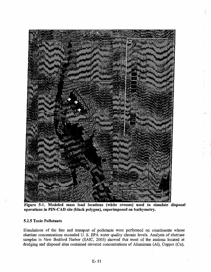
Figure 5-1. Modeled mass load locations (white crosses) used to simulate disposal operations in PIN-CAD site (black polygon), superimposed on bathymetry.

5.2.5 Toxic Pollutants

Simulations of the fate and transport of pollutants were performed on constituents whose elutriate concentrations exceeded U. S. EPA water quality chronic levels. Analysis of elutriate samples in New Bedford Harbor (SAIC, 2003) showed that most of the stations located at dredging and disposal sites contained elevated concentrations of Aluminum (Al), Copper (Cu),

K-51

Nickel (Ni), Silver (Ag) and Polychlorinated Biphenyls (PCB). Benzo(a)fluoranthene and Benzo(k)fluoranthene, part of high molecular weight (HMW) (Petroleum Aromatic Hydrocarbon), also exceeded the USEPA chronic levels at some stations.

As part of modeling input, the mass of the pollutant source is required for each contaminant. Table 5-2 lists the source strengths calculated from equations (1) and (2). Also shown are U. S. EPA water quality chronic criteria and the dilution required to lower elutriate concentrations to meet the criteria.

None of pollutants exceed the U. S. EPA water quality acute level except copper (4.8 ug/L) at NBH-202 and NBH-207 stations. Only Al, Cu, Ag and PCB exceed the chronic levels. The dilution of elutriate concentration for PCB to meet the chronic level ranges between 11 and 67. Copper has the next highest required dilutions (1 to 32) followed by silver (14). Station NBH-202, located at the Channel Inner CAD site, has the highest concentrations for all constituents shown in the table. The next highest concentrations are from station NBH-207, located at Fish Island.

5.2.6 Other Model Parameters

Primary physical processes governing the fate and transport of disposed material are advection and diffusion. The former is due to the currents that are predicted from the hydrodynamic modeling. The latter includes horizontal and vertical diffusion which are specified as model inputs. The vertical diffusion coefficient used was 50 cm /sec (0.05 ft Is), typical of estuary systems (Officer, 1976), and the horizontal diffusion was 1000 cm2/sec (1.09 ft2/s), determined from a dye study in the lower Acushnet estuary (ASA, 2003).

K-52

Table 5-2. Pollutant constituents, elutriate concentrations, source strengths and dilutions for disposal operations at the PIN-CAD site. Dilution is the ratio of elutriate concentration and chronic criteria concentration.

Station

o C N

•

CN O

o CN

i

o CN

o CN

o CN

i

w

Pollutant

Al _ _ C u _

Ni Ag

PCB Al Cu Pb Ni Ag

PCB Al Cu Ni Ag

PCB Al Cu Ni Ag

PCB Al Cu Ni Ag

PCB Al Cu Ni Ag

PCB

Elutriate Cone Gig/L)

161 7.1 13.5 1.4

1.72 2320 97.8 13.4 13.5 L4 23 577

13.5 1.4

0.34 346 10.8 13.5 1.4

216 7.1 13.5 1.4

1.22 853 39

13.5 1.4

5.69

Source Strength

(g) 2021.7 89.2 169.5 17.6 21.6

29132.0 1228.1 1683 169.5 17.6

288.8 7245.3 502 1693 1X6 4.3

4344.7 135.6 169.5 17.6 11.1

2712.3 89.2 169.5 17.6 15.3

10711.0 489.7 169.5 17.6 71.4

WQ Chronic frig/L)

87 3.1 8.2 0.1

0.03 87 3.1 8 l 82 o l

0.03 87 3.1 82 o l 0.03 8 7 s

3.1 8.2 0.1

0.03 87 3.1 8.2 0.1

0.03 87

Ti ~82 " o l 0.03

Dilution

14 "57" ~ ~32~

14 767

14 TT "T"

14 "29"

14

IF IF 14

190

K-53

5.3 BFMASS Modeling Results

This section documents the results of the fate and transport simulations of contaminants disposed at the PIN-CAD site in Inner New Bedford Harbor. Simulations were performed using a three-dimensional (7-layer) application of BFMASS. Three different tides (spring, neap and mean tides), and three wind conditions (calm, northwesterly and southwesterly winds) were chosen as representative of the range of likely environmental conditions.

All modeled constituents were released at the end of flood portion of the M2 tidal cycle, so that the subsequent ebb currents transported the constituents in the water column south toward the Hurricane Barrier.

Elutriate concentration data (Table 5-2) shows that dredged material from station NBH-202 (located at the proposed CAD-CI) was more highly contaminated compared to the other stations. For example, the PCB elutriate concentration was 767 times the U.S. EPA chronic level (U. S. EPA, 2002). This is four times higher than the next highest PCB concentration found at station NBH-207 (located at Fish Island) and 70 times higher than the lowest at station NBH-204 (also located at CAD-CI). This section documents model results in detail for the worst contaminant case, NBH-202 PCBs, and then presents the results in more generalized format for the rest of contaminants and stations.

The BFMASS simulation results indicated that the contaminant distribution patterns in the horizontal and vertical were similar for the three tide ranges. Concentration levels, however, were higher in the near field for neap tides than for spring tides because more energetic currents during the spring tides promote more dispersion and mixing. Different wind conditions resulted in different spatial distribution patterns and coverages. For example, Figure 5-2 PCB shows concentration levels 1 hour after the final disposal event for calm, southwesterly and northwesterly winds. Background hydrodynamics were driven by neap tides. During calm conditions (Figure 5-2a), the simulated plume is more concentric, exhibiting the highest concentration at the release site, whereas the plume is oriented in the down-wind direction forming an elliptic shape (Figures 5-2b and 5-2c). The vertical distribution of contaminant confirms the plume pattern, exhibiting a larger shift toward the down-wind direction at the surface layer than in the lower layers.

Among the three wind conditions, spatial coverage (area exceeding a specified concentration) for the PCB WQ chronic concentration (0.03 ug/L) is the largest for calm wind and the smallest for northwesterly winds. Area coverages appear to have a distinct pattern for different ranges of concentration. Comparing between calm and southwesterly winds, the coverages without wind are larger for concentrations greater than 0.03 ug/L but smaller for lower concentrations. However, for calm conditions, the coverage is larger than for northwesterly winds. Although the same wind speed is applied to Figures 5-5b and 5-5c, smaller area coverages for concentrations larger than 0.05 ug/L and larger coverages for low concentrations (< 0.05 ug/L) are predicted for southwesterly winds (Figure 5-2b). This is due to both tides and southwesterly winds, of which the latter advects contaminants to relatively open and deep areas where the former is also strong.

K-54

i \7 r' 70. a . r f j " 70 a ^ 7B3

i | l ; (A) ..... 0 -{ (BJ < • (C)

i \\ *i \ [ ._ 1

i • v ^ { PCB Cancentialiun I S V

1 1 I (uij/Ll / 1 ;' <r~- \ji < .JC.

• " ' w i ^ tr*' -^t TLEGO' tj"j> .c:i ••• . T i * 1,-r : .̂ , TLEGO' tj"j> .c:i ••• . T i

- i , , ; 4 , M 1 J 1 ' I ' — ' C-j

1 f-S 0- - .23 ^ - i )r~i 1 ; /-" 03 •> " i

: ' r f - . IS-* " WM ^ -̂ - " ^ - s i 1 q F W 1 J E i X SKL i

M"v*\\ 5 -1 .' E3 Sv J, <2v i

1 ^'JCS l-> 3

> 3 s « C ^ ^ r&f£ i i

| 41 MO J '.\ " ""Vfo,

l-> 3

> 3 H H I • f*, fl^ S 41 UU 1 1 , • - ^

1 l V ^Tfeg | 1 i \ -

• V

41 UU 1 1 , • - ^

i

; T l ^ i / / X K - ' i •' i

> / • ^ I / i

i ) t> , « : _ _y i ' ; > - ^ ' . .-J • '' -41 / I i ' ^ " . ^ £' i

i '-J/

; ' , / - v . ^ ' 1 41.G2U J ';

J/

41.G70 ; V 41.GP0 T 1 '• r- JS.I

j J pi ion* | Den Unh„n.

..=<; '.» a1

Clute : 1 Suction Line 1 I

JS.I j

J pi ion* | Den « I Section Line 1 Unh„n.

..=<; '.» • !>ec(iun Line j (Jpfiuns 1 !

| l 7 p

jp£ -* » * • n c- r- , r"

..=<;

C':t

/i1 » / • * * — l i

,

, r"

..=<;

1 , -T . • I L _ c • b i « -T.- " • aj li !

Figure 5-2. Simulated PCB distributions for calm wind (a), southwesterly (b) and northwesterly winds (c). Distributions are shown 1 hour after the final disposal event.

Among the nine environmental scenarios, the largest spatial coverage was predicted for neap tides and calm wind conditions. On the other hand, the smallest coverage occurred for neap tides and northwesterly winds. This finding was consistent among the three different release locations in the PIN-Cad cell. Figures 5-3 and 5-4 show the maximum area affected (coverage) due to released NBH-202 PCB as a function of concentration for the neap tide and no wind condition and the neap tide and northwesterly wind condition, respectively. The area of the PIN-CAD is shown for reference as is the U. S. EPA chronic water quality (WQ) concentration for PCB.

Under calm winds (Figure 5-3), concentrations less than 0.4 ug/L.

the area coverage is always larger than the CAD area for The coverages at the PCB chronic level (0.03 ug/L) are lxlO6

mz (southeast corner release) and 1.2><106 m2 (center and northwest corner releases), which are between 6 and 7 times larger than the CAD cell area, respectively. The concentrations for an area the same as the CAD site area are 0.42 ug/L, 0.44 ug/L and 0.35 pig/L for a center, northwest and southeast release, respectively. While the calm wind condition simulates very similar coverages for the three release locations (Figure 5-3), a northwest release with northwesterly winds generates the largest coverage and a southeast release yields the smallest coverage (Figure 5-4). Spatial coverage for the 0.03

K-55

M ax im u m Area Coverage of Released NBH-202 P C B for Neap T ide and No W i n d Condit ion

2 1.E+05

Simulated PCB Concentration (ug/L)

Figure 5-3. Maximum area coverages (y-axis) of PCBs vs. concentrations for neap tides and calm winds for three release sites using the NBH-202 station source strength. Both x- and y-axes are logarithmic scales. The PIN-CAD cell area (1.67xl05 m2) is shown with a black horizontal line and the U. S. EPA WQ chronic value for PCB (0.03 u.g/L) is shown with a dashed vertical line.

M a x i m u m Area Coverage of Released NBH-202 P C B for Neap T ide and Northwester ly W i n d Condi t ion

Simulated PCB Concentration (ug/L)

Figure 5-4. Maximum area coverages (y-axis) of PCBs vs. concentrations for neap tides and northwesterly winds for three release sites using the NBH-202 station source strength. Both x- and y-axis are logarithmic scale. The PIN-CAD cell area (1.67x10s m2) is shown with a black horizontal line and the U. S. EPA WQ chronic value for PCB (0.03 fig/L) is shown with a dashed vertical line.

K-56

ug/L chronic concentration with wind is 0.3xlO6 m2, 1.9xl05 m2, and 3.3xlO6 m2 with southeast, center and northwest releases, respectively. The concentrations for areas equivalent to the CAD site area are 0.015 ug/L for a southeast release, 0.035 ug/L for a center release and 0.08 ug/L for a northwest release.

Figure 5-5a presents the same area coverages as Figure 5-3, except concentrations are shown relative to a unit input mass (g). In other words, Figure 5-3 can be obtained by multiplying the concentrations in Figure 5-5a by 288.8 (PCB source strength for NBH-202). The advantage of presenting the results in this way is that the simulated coverage is not pollutant- or site-specific. Hence, the results can be applied to any pollutant and any station by multiplying by the corresponding source strength listed in Table 5-2. Ni and Pb chronic criteria are almost identical so the Pb is not presented in the figure.

For example, using aluminum (Al) originating from station NBH-201, the concentration having the same size as the CAD cell is 3 ug/L ( 0.00158 ug/L x 2021.7) with the southeast corner release (red curve in Figure 5-5a). Areas for concentrations greater than 3 ug/L are smaller than the CAD cell. The coverage for the Al WQ chronic concentration (87 ug/L) is 5.5X10 m2. Similarly for the center (blue in Figure 5-5a) and northwest releases (green in Figure 5-5a), the concentration covering the same size as the CAD cell is 2.5 ug/L (0.00126 ug/L x 2021.7) and spatial coverage for the chronic concentration is 2.2xl04 m2.

Overall, for neap tide and calm wind conditions both Al and Cu exhibit smaller area coverages than the CAD cell. Area coverage for Ag is either the same as or slightly larger than the area of the release cell (shown as the horizontal tail end of each curve). For Pb and Ni, predicted concentrations in the release cell are below the chronic level.

Figures 5-b and 5-c are the same as Figure 5-a, except for different wind directions, southwesterly and northwesterly, respectively. The difference between the two wind conditions is that the area coverage for southwesterly winds is almost constant for low concentrations and gradually decreases for high concentrations, whereas the coverage for northwesterly winds linearly decreases with concentrations. The coverages for Al, Cu and Ag chronic concentrations are smaller than the CAD cell size for both wind conditions. Predicted concentrations of Pb and Ni are always smaller than their chronic concentrations while PCB concentrations are larger.

During neap tides and calm winds (Figure 5-5a), the coverage is almost same regardless of release site. With winds (Figures 5-5b and 5-5c), the southeast corner release exhibits the largest coverage for southwesterly winds and the smallest coverage for northwesterly winds. The opposite exists for a northwest corner release, with a large coverage for southwesterly winds and small coverage for northwesterly winds.

Figure 5-6 shows maximum area coverages for spring tides and the three different wind conditions. Individual spatial coverage curves for spring tides appear very similar to those for neap tides (Figure 5-5). However, a comparison between Figures 5-5b and 5-6b for southwesterly winds shows that smaller coverages for spring tides are found with a southeast release, and relatively larger coverages for spring tides are predicted with a

K-57

Figure 5-5. Maximum area coverages (solid lines) for neap tides and calm (a), southwesterly (b) and northwesterly winds (c). Dashed lines denote U. S. EPA WQ chronic concentrations normalized to input mass.

K-58

(A) Maximum Area Coverage of Released Contaminant for Spring Tide and No Wind Condition

: : : : : : : : : : : : j : : : : : 3 3 S » 3 3 S »

:::::::ti:::"T":: ::::::::::::r:::: 11 1... II i

J . . . . i

1 E-KJ6

11 1... II i

J . . . . i

1 E-KJ6 :::::::U:::::t:" : : : : : : : : : : : : ] : : : : : :::::: : f i : : : :?: : : :::::::::::: j : : : : : :::::: : f i : : : :?: : : :::::::::::: j : : : : :

V—--fi—-|—- 1

I \ \ I I f 1 • — — C e n t e r

™ — — NW comer

PIN-CAD

PCB W Q level

Al WQ level

Cu WO level

Pfa WQ level

Ni WQ level

Ag W Q level

— — C e n t e r

™ — — NW comer

PIN-CAD

PCB W Q level

Al WQ level

Cu WO level

Pfa WQ level

Ni WQ level

Ag W Q level

— — C e n t e r

™ — — NW comer

PIN-CAD

PCB W Q level

Al WQ level

Cu WO level

Pfa WQ level

Ni WQ level

Ag W Q level

— — C e n t e r

™ — — NW comer

PIN-CAD

PCB W Q level

Al WQ level

Cu WO level

Pfa WQ level

Ni WQ level

Ag W Q level

— — C e n t e r

™ — — NW comer

PIN-CAD

PCB W Q level

Al WQ level

Cu WO level

Pfa WQ level

Ni WQ level

Ag W Q level

v&t >

— — C e n t e r

™ — — NW comer

PIN-CAD

PCB W Q level

Al WQ level

Cu WO level

Pfa WQ level

Ni WQ level

Ag W Q level

1.E-HD4 :

— — C e n t e r

™ — — NW comer

PIN-CAD

PCB W Q level

Al WQ level

Cu WO level

Pfa WQ level

Ni WQ level

Ag W Q level

•VS ! 1

:

— — C e n t e r

™ — — NW comer

PIN-CAD

PCB W Q level

Al WQ level

Cu WO level

Pfa WQ level

Ni WQ level

Ag W Q level

::::::tiiw-::: : : : : : : : : : : :£:::: :

— — C e n t e r

™ — — NW comer

PIN-CAD

PCB W Q level

Al WQ level

Cu WO level

Pfa WQ level

Ni WQ level

Ag W Q level

— — C e n t e r

™ — — NW comer

PIN-CAD

PCB W Q level

Al WQ level

Cu WO level

Pfa WQ level

Ni WQ level

Ag W Q level N""nii. — 1

— — C e n t e r

™ — — NW comer

PIN-CAD

PCB W Q level

Al WQ level

Cu WO level

Pfa WQ level

Ni WQ level

Ag W Q level .11... i . „ . 1

| " !!..!... !

(B) Maximum Area Coverage of Released Contaminant for Spring Tide and Southwesterly Wind Condition

0.G001 0.001 0.01

Simulated Concentration (ug/L) to Unit Mass (

(C) Maximum Area Coverage of Released Contaminant for Spring Tide and Northwesterly Wind Condition

:^?^sr : ; : : : : : : : = =!=!==H=p-|H==^n=== :::"::"ci""T*" " " : : : . : : : : : : ] : : : : :

u t j . .. It ! i

sp^n i ; "**1^N

M-—4- i "̂̂ "**1^N

M-—4- i

fI—-T— i

V \ Jl t i 1,6405;

Center

— — — NW corner

5 E comer

PIN-CAD

PCB W O level

Al WQ level

Cu W Q level

Pb W Q level

Ni W Q level

A g W Q level

: : : : : : : f j : : : :?::: Center

— — — NW corner

5 E comer

PIN-CAD

PCB W O level

Al WQ level

Cu W Q level

Pb W Q level

Ni W Q level

A g W Q level

Center

— — — NW corner

5 E comer

PIN-CAD

PCB W O level

Al WQ level

Cu W Q level

Pb W Q level

Ni W Q level

A g W Q level

Center

— — — NW corner

5 E comer

PIN-CAD

PCB W O level

Al WQ level

Cu W Q level

Pb W Q level

Ni W Q level

A g W Q level

Center

— — — NW corner

5 E comer

PIN-CAD

PCB W O level

Al WQ level

Cu W Q level

Pb W Q level

Ni W Q level

A g W Q level

Center

— — — NW corner

5 E comer

PIN-CAD

PCB W O level

Al WQ level

Cu W Q level

Pb W Q level

Ni W Q level

A g W Q level

—SJ1 I i

Center

— — — NW corner

5 E comer

PIN-CAD

PCB W O level

Al WQ level

Cu W Q level

Pb W Q level

Ni W Q level

A g W Q level

EEEEEXKIEEEEEEEE:

Center

— — — NW corner

5 E comer

PIN-CAD

PCB W O level

Al WQ level

Cu W Q level

Pb W Q level

Ni W Q level

A g W Q level

Center

— — — NW corner

5 E comer

PIN-CAD

PCB W O level

Al WQ level

Cu W Q level

Pb W Q level

Ni W Q level

A g W Q level

Center

— — — NW corner

5 E comer

PIN-CAD

PCB W O level

Al WQ level

Cu W Q level

Pb W Q level

Ni W Q level

A g W Q level rtTC .• 1 j

Center

— — — NW corner

5 E comer

PIN-CAD

PCB W O level

Al WQ level

Cu W Q level

Pb W Q level

Ni W Q level

A g W Q level 1.1 L... j

j | I I 1 — . ' I ,'.,,,

i

Figure 5-6. Maximum area coverages (solid lines) for spring tides and calm (a), southwesterly (b) and northwesterly winds (c). Dashed lines denote U. S. EPA WQ chronic concentrations normalized to input mass.

K-59

northwest release. For northwesterly winds between neap (Figure 5-5c) and spring (Figure 5-6c) tides, the coverage with a northwest release was the same for both tides but relatively larger coverage occurs for spring tides than neap tides with a southeast release.

Figure 5-7 shows maximum spatial coverages for mean tides and the three wind conditions. Variations in area coverage consistently lie between neap and spring tides, as expected.

According to toxicity tests using sediments from the stations listed in Table 5-2 with mysids and sea urchins reported by SAIC (2003), the cause of acute toxicity was the combination of multiple pollutants. For example, half the toxicity to mysids was due to PCBs and the other half was due to a combination of copper and ammonia. From these results, SAIC suggested that a dilution to at least 2.2% of the elutriate concentration would be protective.

Figure 5-8 shows maximum area coverages for a release of lg of a combination of toxic pollutants. Presented are the coverages for the worst conditions (neap tide and calm wind) and the most favorable conditions (neap tide and northwesterly wind). For both conditions, area coverage for a concentration of 2.2% of the elutriate level was always smaller than the PIN-CAD area. The largest area coverage for the 2.2% elutriate concentration occurred for a northwest release during calm winds, 1.2><105 m2. The smallest coverage for the protective dilution level occurred for a southeast release during northwesterly winds, 1.0x104 m2.

K-60

(A) Maximum Area Coverage of Released Contaminant

for Mean Tide and No Wind Condition

0.0001 0.001 0.01

Simulated Concentration (ug/L) to Unit Mass (g)

for Mean Tide and Northwesterly Condition

0.0001 0.001 0.01

Simulated Concentration (ug/L) to Unit Mass (g)

I.C-MJ/

? « ! * * : rr 1 ::::::::::::)::::: ? « ! * *

u i _ i . I I 1 i

, j

k"""n" T i

\ '' r i

— — M W corner

S E corner

PIN-CAD

PCB W Q level

A l W O level

Cu W O level

Pb W Q level

— — Ni W Q level

— — A g W Q level

:;::^;ti" :$:::: : : : : : : : : : : : : E j : : : : : ::::::::::::::::::: — — M W corner

S E corner

PIN-CAD

PCB W Q level

A l W O level

Cu W O level

Pb W Q level

— — Ni W Q level

— — A g W Q level

— — M W corner

S E corner

PIN-CAD

PCB W Q level

A l W O level

Cu W O level

Pb W Q level

— — Ni W Q level

— — A g W Q level

— — M W corner

S E corner

PIN-CAD

PCB W Q level

A l W O level

Cu W O level

Pb W Q level

— — Ni W Q level

— — A g W Q level

— — M W corner

S E corner

PIN-CAD

PCB W Q level

A l W O level

Cu W O level

Pb W Q level

— — Ni W Q level

— — A g W Q level

— — M W corner

S E corner

PIN-CAD

PCB W Q level

A l W O level

Cu W O level

Pb W Q level

— — Ni W Q level

— — A g W Q level

i | \ i 1 1.E-KJ4 .

— — M W corner

S E corner

PIN-CAD

PCB W Q level

A l W O level

Cu W O level

Pb W Q level

— — Ni W Q level

— — A g W Q level

::::::H:\ : l : : : : : : : : : : : : : : : ] : : : : : :

— — M W corner

S E corner

PIN-CAD

PCB W Q level

A l W O level

Cu W O level

Pb W Q level

— — Ni W Q level

— — A g W Q level

— — M W corner

S E corner

PIN-CAD

PCB W Q level

A l W O level

Cu W O level

Pb W Q level

— — Ni W Q level

— — A g W Q level

— — M W corner

S E corner

PIN-CAD

PCB W Q level

A l W O level

Cu W O level

Pb W Q level

— — Ni W Q level

— — A g W Q level

— — M W corner

S E corner

PIN-CAD

PCB W Q level

A l W O level

Cu W O level

Pb W Q level

— — Ni W Q level

— — A g W Q level r i""n£; — 1

— — M W corner

S E corner

PIN-CAD

PCB W Q level

A l W O level

Cu W O level

Pb W Q level

— — Ni W Q level

— — A g W Q level u... « . . . . . J . . . . . .

1 E-H33 - ... r., :;r::;::; II 1 1 1 . M , , • , , „ . . , , '

(B) Maximum Area Coverage of Released Contaminant

for Mean Tide and Southwesterly Wind Condition

::::::::::::::::::: : : E : E : EE : E : :EE : :E EEEEEEEHEEEEEEEEE EEEEEEEEEEEE3EEEEE

5? : : [ ! : ; i : : 1

1.E-HDS

^ N 5? U....JL...

I I !

. . . J

1 1.E-HDS

= ! ! s ! = i i i : : : : : : : » : : : : ? " - • : : : : : : : : : : : : ? : : : : :

::::::::::::::v" ••—V-V-—-\ r]—-T— I

V \ \ 1 J 1.E405 Center

-——— N W corner

'SE comer

PIN-CAD

PCB W Q level

A l W O level

Cu W Q level

Pb W Q level

Ni W Q level

A g W O level

EEEEEIEEEEEEE^EEEEjEE : : : : : - - : f l : : : : * : : : : EEEEEEEEEEEEEEEEEEE Center

-——— N W corner

'SE comer

PIN-CAD

PCB W Q level

A l W O level

Cu W Q level

Pb W Q level

Ni W Q level

A g W O level

t - ^ v f i—-+—• 1

Center

-——— N W corner

'SE comer

PIN-CAD

PCB W Q level

A l W O level

Cu W Q level

Pb W Q level

Ni W Q level

A g W O level

u—-+—•

fV--H—-+—-\ \ l l s i

Center

-——— N W corner

'SE comer

PIN-CAD

PCB W Q level

A l W O level

Cu W Q level

Pb W Q level

Ni W Q level

A g W O level

Vj-—• u—-+—•

fV--H—-+—-\ \ l l s i

:

Center

-——— N W corner

'SE comer

PIN-CAD

PCB W Q level

A l W O level

Cu W Q level

Pb W Q level

Ni W Q level

A g W O level

::::: %::^ j : : : : j : : : : : : : : : : : : : : : : : j : : : : : :

Center

-——— N W corner

'SE comer

PIN-CAD

PCB W Q level

A l W O level

Cu W Q level

Pb W Q level

Ni W Q level

A g W O level

::::H&:£:::: : : : : : : : : : : : £ : : : : •

Center

-——— N W corner

'SE comer

PIN-CAD

PCB W Q level

A l W O level

Cu W Q level

Pb W Q level

Ni W Q level

A g W O level

Center

-——— N W corner

'SE comer

PIN-CAD

PCB W Q level

A l W O level

Cu W Q level

Pb W Q level

Ni W Q level

A g W O level r r ' ^s^ ; ^z: 1

Center

-——— N W corner

'SE comer

PIN-CAD

PCB W Q level

A l W O level

Cu W Q level

Pb W Q level

Ni W Q level

A g W O level I I JL_... J

1.E-W3 4- [ I I I I I

, U , , . ! , , . i • . ,.', . . . .

Figure 5-7. Maximum area coverages (solid lines) for mean tides and calm (a), southwesterly (b) and northwesterly winds (c). Dashed lines denote U. S. EPA WQ chronic concentrations normalized to input mass.

K-61

Maximum Area Coverages

1.E+07

1.E+06

1.E+05

1.E+04

1.E+03

—Calm-Center

—Calm-Northwest

-—-Calm-Southeast

Northwesterly-Center

Northwesterly-Northwest

Northwesterly-Southeast

PIN-CAD

2.2% dilution

U -0.000001 0.00001 0.0001 0.001 0.01

Simulated Concentration (ug/L) to Unit Toxic Mass

0.1

Figure 5-8. Maximum area coverage for released toxic material for calm and northwesterly winds.

6. Summary and Conclusions

The field-obtained elevations and velocities were examined to determine that tides and wind were the primary forces that drove the circulation in New Bedford Harbor. Hydrodynamic simulations were successfully conducted to verify model performance for the period of the field measurement program. Nine basic hydrodynamic conditions were prepared to provide the advection data to the pollutant and sediment transport models based on the combination of three tidal ranges (neap, mean and spring) and three most likely wind conditions (calm, southwesterly and northwesterly directions).

The SSFATE (Suspended Sediment Fate) model was used to simulate TSS (Total Suspended Solid) concentrations due to the proposed excavation of the CAD (Confined Aquatic Disposal) cells and the disposal of dredged material into one of the cells. Resultant TSS distributions showed that combinations of the wind induced circulation and bathymetry played a key role. When the sediment plumes were carried into the deeper sections of the harbor, the duration and size of sediment cloud were more extensive than when the sediment plumes were carried into the shallower sections, where the sediment settled out more quickly.

A series of dissolved phase pollutant fate and transport simulations were performed to estimate the water quality impacts in the water column at north of Popes Island, using BFMASS (Boundary Fitted Mass Transport Model). Simulations were performed for various pollutant

K-62

constituents whose elutriate concentrations exceeded the U. S. EPA water quality guidance levels: metals (aluminum, copper, nickel and silver), and polychlorinated biphenyls (PCBs). The model simulated the fate and transport of disposal of dredged material at the PIN-CAD site (north of Popes Island). Disposal operations were assumed to last for 6 days and disposal taking place twice a day following the M2 tidal cycle. Each release volume of dredged material was assumed to be 1,530 m3 (2,000 yd3).

None of pollutant elutriate concentrations exceeded the U. S. EPA water quality acute criteria except copper (4.8 ug/L) at two stations. Al, Cu, Ni, Ag, and PCB exceed chronic levels. The dilution of elutriate concentration for PCB to meet the chronic criteria ranged between 11 and 767, Cu had the next highest required dilutions (1 to 32) followed by Al (2 to 27), Ag (14) and Ni (2). One proposed site, Station NBH-202, located at another proposed CAD site denoted Channel Inner (CAD-CI), had the highest concentrations for all constituents. Station NBH-207, located north of Fish Island, was second highest.

The BFMASS simulation results indicated that the contaminant distribution patterns in the horizontal and vertical were similar for the three tide ranges. Concentration levels, however, were higher in the near field for neap tides than for spring tides because more energetic currents during the spring tides promote more dispersion and mixing. Different wind conditions resulted in different spatial distribution patterns and coverages. Among the nine environmental scenarios, the largest spatial coverage (area) was predicted for neap tides and calm wind conditions. The smallest coverage occurred for neap tides and northwesterly winds. This finding was consistent among three different release locations in the large PTN-CAD cell.

According to toxicity tests using sediments from the NBH-202 station sampled at CAD-CI, the combination of multiple pollutants was the cause of the observed acute toxicity effects. For example, half the toxicity to mysids was due to PCBs and the other half was due to a combination of copper and ammonia. From these results S AIC concluded a dilution to less than 2.2% of the elutriate concentration would be protective. The model results showed that for any environmental condition, area coverage for a concentration of 2.2% of the elutriate level was always smaller than the PIN-CAD area (1.67x105 m2 [41 ac]). The largest area coverage (1.2x105 m2 [30 ac]) of the 2.2% elutriate concentration occurred for a release during calm conditions while the smallest coverage (1.0x104 m2 [2.5 ac]) occurred for a release during northwesterly winds. Other sediments with lower elutriate concentrations, and presumably lower toxicity, would affect smaller areas.

K-63

7. References

Abdelrhman, M. A. and E. H. Dettmann, 1995. Modeling of current circulation, residence time, and salinity distribution in New Bedford Harbor, MA. U. S. Environmental Protection Agency, Environmental Research Laboratory, Narragansett, RI.

Abdelrhman, M.A., Modeling How a Hurricane Barrier in New Bedford Harbor, Massachusetts, Affects the Hydrodynamics and Residence Times, Estuaries, Vol. 25. No. 2, P. 177-196, April 2002.

Ambrose, R.B. et al, 1993. The Water Quality Analysis Simulation Program, WASP5 Part A: Model Documentation, Part B: The WASP5 Input Data Set. U.S. Environmental Protection Agency, Athens, GA.

Anderson, E., B. Johnson, T. Isaji and E. Howlett, 2001. SSFATE (Suspended Sediment FATE), a model of sediment movement from dredging operations. Presented at WODCON XVI World Dredging Congress, 2-5 April 2001, Kuala Lumpur, Malaysia.

Applied Science Associates, Inc, 1987. Selected studies of PCB transport in New Bedford Harbor. Applied Science Associates, Inc., Narragansett, RI. 193 pp..

Applied Science Associates, Inc., 1999. User's Technical Manual for WQMAP for Windows. Applied Science Associates, Inc. 126 pp.

Applied Science Associates, Inc, 2001. ASA 01-100 Report: Preliminary Dredged Material Transport Modeling in New Bedford Harbor. 30pp.

Applied Science Associates, Inc, 2003. Flushing Analysis in the Acushnet River Estuary. ASA Report 01-123. 138pp.

Averett, D. E., 1989. New Bedford Harbor Superfund Project, Acushnet River Estuary Engineering Feasibility Study of Dredging and Dredged Material Disposal Alternatives, Report 3, Characterization and Elutriate Testing of Acushnet River Estuary Sediment. Technical Report EL-88-15. Waterways Experiment Station, Corps of Engineers, Vicksburg, Mississippi.

Collection (TN DOER-E12). U.S. Army Engineer Research and Development Center, Vicksburg, MS. http: //www.wes.army.mil/el/dots/doer/pdf/doerel2.pdf.

Coastal Zone Management, City of New Bedford and Town of Fairhaven, 2002. Draft Environmental Impact Report (DEIR) for New Bedford and Fairhaven Massachusetts. Dredged Material Management Plan (DMMP) EOEA No. 11669.

DOER Technical Notes Collection (TN DOER-E10). U.S. Army Engineer Research and Development Center, Vicksburg, MS. http: //www.wes.army.mil/el/dots/doer/pdf/doerelO.pdf.

K-64

ENSR, International, 2002. Boston Harbor Navigation Improvement Project Phase 2 Summary Report.

Galagan C , Swanson, C, and T. Isaji, 2001. Simulations of Sediment Transport and Deposition from Jet Plow and Excavation Operations for the Cross Hudson Project, Prepared for Environmental Science Services, Inc. Wellesley, MA. ASA Project 99-063.

Johnson, B. H., 1990. User's guide for models of dredged material disposal in open water. Technical Report D-90-5. Waterways Experiment Station, Corps of Engineers, Vicksburg, Mississippi.

Johnson, B.H., E. Anderson, T. Isaji, and D.G. Clarke, 2000. Description of the SSFATE numerical modeling system.

Malcolm Pirnie, Inc. 1982. The Commonwealth of Massachusetts. Acushnet River Estuary, PCB Study. December 1982.

Mendelsohn, D, T. Isaji and H. Rines, 1995. Hydrodynamic and water quality modeling of Lake Champlain. Report to Lake Champlain Management Conference, Burlington, VT, ASA Report 92-034.

Muin, M. 1993. A Three-Dimensional Boundary Fitted Circulation Model in Spherical Coordinates. Ph. D. Dissertation, Department of Ocean Engineering, University of Rhode Island, Kingston, RI.

Muin, M. and M. L. Spaulding, 1996. Two-dimensional boundary fitted circulation model in spherical coordinates. In: Journal of Hydraulic Engineering, Vol. 122, No. 9, September 1996, and p. 512-521.

Muin, M. and M. L. Spaulding, 1997a. Application of Three-dimensional boundary fitted circulation model to Providence River. ASCE Journal of Hydraulic Engineering. Vol. 123, No. 1.

Muin, M. and M. L. Spaulding, 1997b. Three-dimensional boundary fitted circulation model. In: Journal of Hydraulic Engineering, Vol. 123, No. 1, pp. 2-12. Officer, C. B., 1976. Physical Oceanography of Estuaries (and Associated Coastal Waters). John Wiley & Sons. 465pp.

National Geophysical Data Center, GEOphysical Data System for Hydrographic Survey Data, National Ocean Service, Ver. 4. 1998

NUS. 1984. Draft Feasibility Study of the Remedial Action Alternatives - Acushnet River Estuary Above Coggeshall Street Bridge, New Bedford, Massachusetts.

SAIC, 2002. Laboratory Testing in Support of Site Specific Water Quality Criteria Assessment and Hydrographic Data Collection for New Bedford Harbor, Task 2A, Suspended Particulate

K-65

Phase Toxicity Testing with Mysids, Data Report. Submitted by Science Applications International Corporation, Newport, RI, 12 December 2002.

Signell, R. 1987. Tide- and Wind-Forced Currents in Buzzards Bay, Massachusetts. WHQI-87-15 Technical Report, pp 86.

Swanson, J. C , 1986. A three dimensional numerical model system of coastal circulation and water quality. Ph. D. Thesis, Dept. of Ocean Engineering, University of Rhode Island, Kingston, RI.

Swanson, J.C., D. Mendelsohn, 1993. Application of WQMAP to upper Narragansett Bay, Rhode Island. Estuarine and Coastal Modeling III. Proceedings of the 3rd

International Conference, sponsored by the Waterway, Port, Coastal and Ocean Division of the ASCE, Oak Brook, IE, September 8-10, 1993.

Swanson, C. J., and D. Mendelsohn, 1995. Modeling Results to Assess Water Quality Impacts from Dredged Material Disposal Operations for the Boston Harbor Navigation Improvement Project. Applied Science Associates, Inc. 53pp.

Swanson, J. C , and D. Mendelsohn, 1996. Water quality impacts of dredging and disposal operations in Boston Harbor. Presented at: ASCE North American Water and Environmental Congress '96 (NAWEC '96), Anaheim, CA, June 22-28, 1996.

Spaulding, M., D. Mendelsohn and J.C. Swanson, 1999. WQMAP: An integrated three-dimensional hydrodynamic and water quality model system for estuarine and coastal applications. Marine Technology Society Journal, Vol. 33, No. 3, pp. 38-54, Fall 1999.

Swanson, C.J., T. Isaji, and M. Ward, 2000. Dredged Material Plume for the Providence River and Harbor Maintenance Dredging Project. Prepared for New England District, U.S Army Corps of Engineers, Concord, MA, ASA Project 99-063.

Swanson, J.C, T. Isaji, M. Ward, B.H. Johnson, A. Teeter, and D.G. Clarke, 2000. Demonstration of the SSFATE numerical modeling system. DOER Technical Notes

Swanson, C, C. Galagan, T. Isaji and H.-S. Kim, 2001. Simulations of sediment deposition from jet plow operations in New Haven Harbor. Draft Final Report to Environmental Science Services, July 2001, 13p.

U. S. Army of Corps of Engineers and Massachusetts Port Authority, 1995. Final Environmental Impact Report and Final Environmental Impact Statement: Boston Harbor, Massachusetts, Navigational Improvement Project and Berth Dredging Project. Volumes 1 through 3.

U. S. EPA, 1991. Evaluation of dredged material proposed for ocean disposal (testing manual). EPA 503/6-91/001, Environmental Protection Agency and Department of the Army. Washington, DC.

K-66