new and best-practice approaches to thresholding

1

New and best-practice approaches

to thresholding

Thomas Nichols, Ph.D. Department of Statistics &

Warwick Manufacturing Group University of Warwick

FIL SPM Course 17 May, 2012

Overview

•  Why threshold? •  Assessing statistic images •  Measuring false positives •  Practical solutions

2

Thresholding

Where’s the signal?

t > 0.5 t > 3.5 t > 5.5

High Threshold Med. Threshold Low Threshold

Good Specificity

Poor Power (risk of false negatives)

Poor Specificity (risk of false positives)

Good Power

...but why threshold?!

4

•  Don’t threshold, model the signal! – Signal location?

•  Estimates and CI’s on (x,y,z) location

– Signal magnitude? •  CI’s on % change

– Spatial extent? •  Estimates and CI’s on activation volume •  Robust to choice of cluster definition

•  ...but this requires an explicit spatial model

Blue-sky inference: What we’d like

space

Loc.θ̂ Ext.θ̂

Mag.θ̂

5

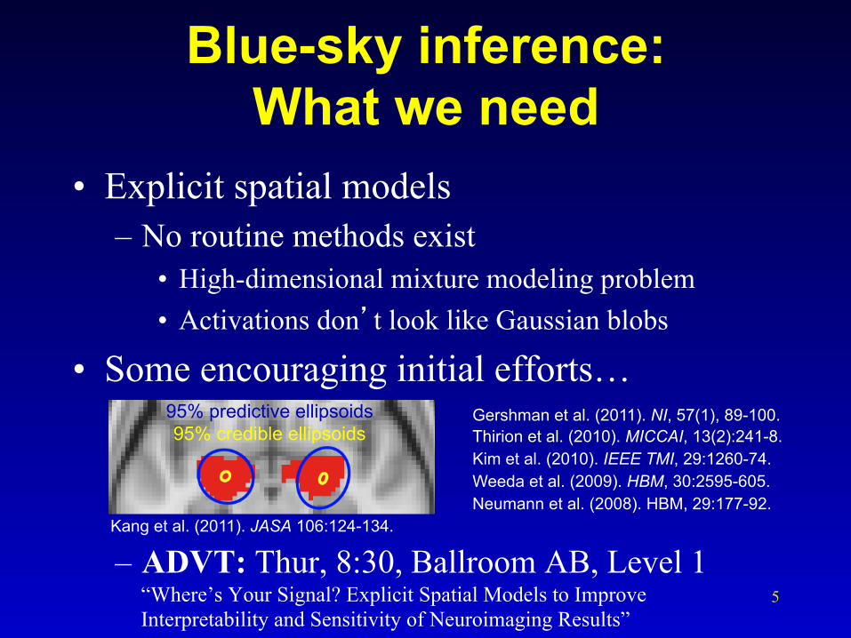
Blue-sky inference: What we need

•  Explicit spatial models – No routine methods exist

•  High-dimensional mixture modeling problem •  Activations don’t look like Gaussian blobs

•  Some encouraging initial efforts…

– ADVT: Thur, 8:30, Ballroom AB, Level 1 “Where’s Your Signal? Explicit Spatial Models to Improve Interpretability and Sensitivity of Neuroimaging Results”

Gershman et al. (2011). NI, 57(1), 89-100. Thirion et al. (2010). MICCAI, 13(2):241-8. Kim et al. (2010). IEEE TMI, 29:1260-74. Weeda et al. (2009). HBM, 30:2595-605. Neumann et al. (2008). HBM, 29:177-92.

Kang et al. (2011). JASA 106:124-134.

95% predictive ellipsoids 95% credible ellipsoids

6

Real-life inference: What we get (typically)

•  Signal location – Local maximum – no inference

•  Signal magnitude – Local maximum intensity – P-values (& CI’s)

•  Spatial extent – Cluster volume – P-value, no CI’s

•  Sensitive to blob-defining-threshold

7

Assessing Statistic Images…

Ways of assessing statistic images

•  Standard methods – Voxel – Cluster – Set – Peak (new)

8

9

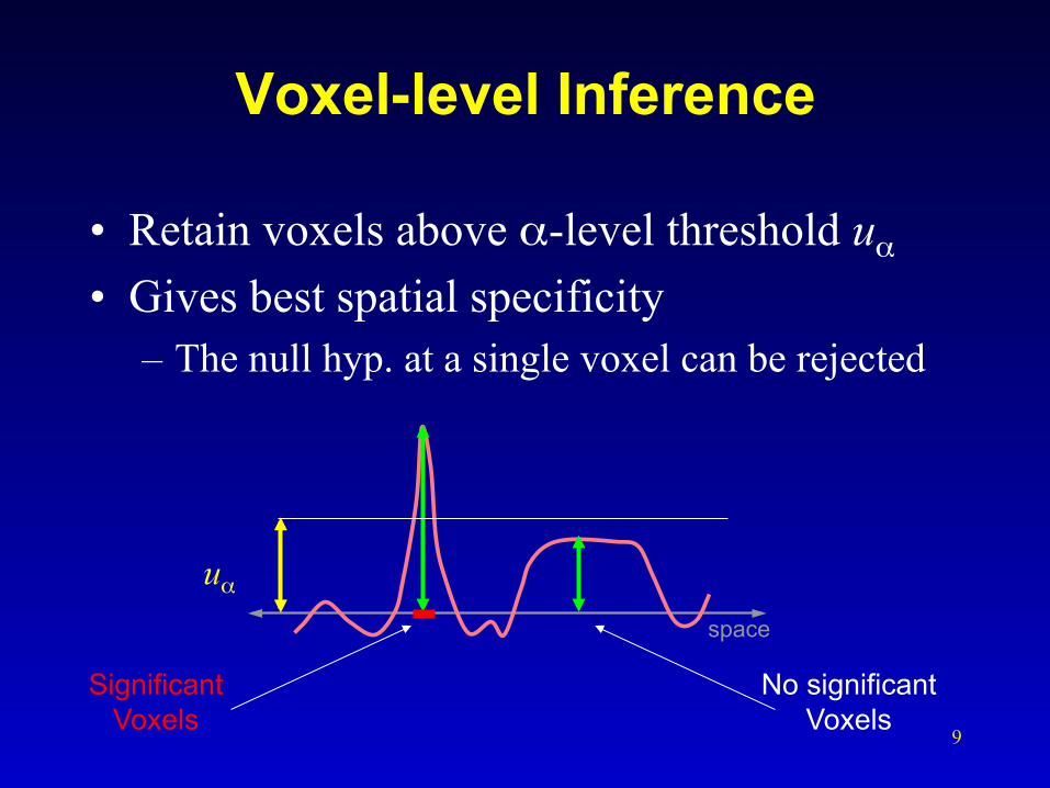
Voxel-level Inference

•  Retain voxels above α-level threshold uα

•  Gives best spatial specificity – The null hyp. at a single voxel can be rejected

Significant Voxels

space

uα

No significant Voxels

10

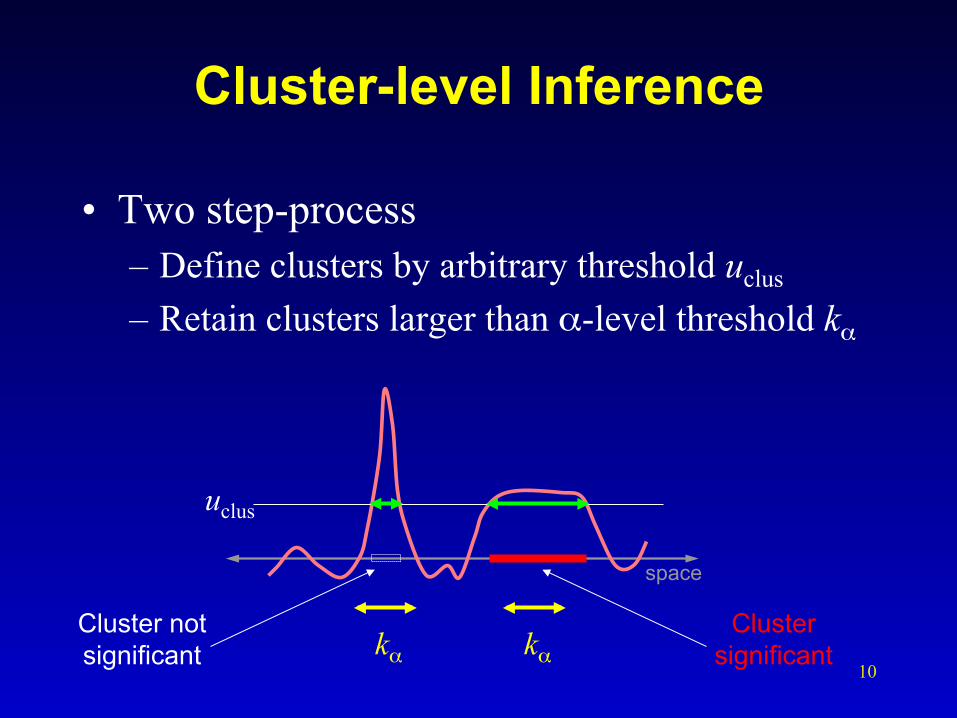
Cluster-level Inference

•  Two step-process – Define clusters by arbitrary threshold uclus

– Retain clusters larger than α-level threshold kα

Cluster not significant

uclus

space

Cluster significant kα kα

11

Cluster-level Inference

•  Typically better sensitivity •  Worse spatial specificity

– The null hyp. of entire cluster is rejected – Only means that one or more of voxels in

cluster active

Cluster not significant

uclus

space

Cluster significant kα kα

12

Set-level Inference

•  Count number of blobs c – Minimum blob size k

•  Worst spatial specificity – Only can reject global null hypothesis

uclus

space

Here c = 1; only 1 cluster larger than k

k k

13

Peak-level Inference

•  Identify all the local maxima –  Ignore all smaller than upeak

•  Retain peaks by height

Significant peak

space

upeak

Not a significant peak

uα

14

Peak-level Inference

•  “Topological inference” – interpretable with boundless Point Spread Function (see Chumbley & Friston, NI, 2009)

•  Cumbersome – only making inference at a sprinkling of locations

Significant peak

space

upeak

Not a significant peak

uα

15

Test Statistics for Assessing Statistic

Images…

Sometimes, Different Possible Ways to Test…

16

Image Feature Test Statistic Voxel 1.  Statistic image value Cluster 1.  Cluster size in voxels

2.  Cluster size in RESELs 3.  Combination, Joint Peak-Cluster 4.  Combination, Cluster Mass 5.  Combination, Threshold-Free Cluster

Enhancement Set 1.  Cluster count Peak 1.  Statistic image value

Sometimes, Different Possible Ways to Test…

17

Image Feature Test Statistic Voxel 1.  Statistic image value Cluster 1.  Cluster size in voxels

2.  Cluster size in RESELs 3.  Combination, Joint Peak-Cluster 4.  Combination, Cluster Mass 5.  Combination, Threshold-Free Cluster

Enhancement Set 1.  Cluster count Peak 1.  Statistic image value

Combining Cluster Size with Intensity Information

•  Peak-Height combining Poline et al., NeuroImage 1997

– Minimum Pextent & Pheight •  Take better of two P-values;

(use RFT to correct for taking minimum) – Can catch small,

intense clusters

•  Cluster mass Bullmore et al., IEEE Trans Med Img 1999 –  Integral M above threshold

•  More powerfully combines peak & height (Hayasaka & Nichols, NI 2004)

•  Both are still cluster inference methods!

space

uc

space

uc

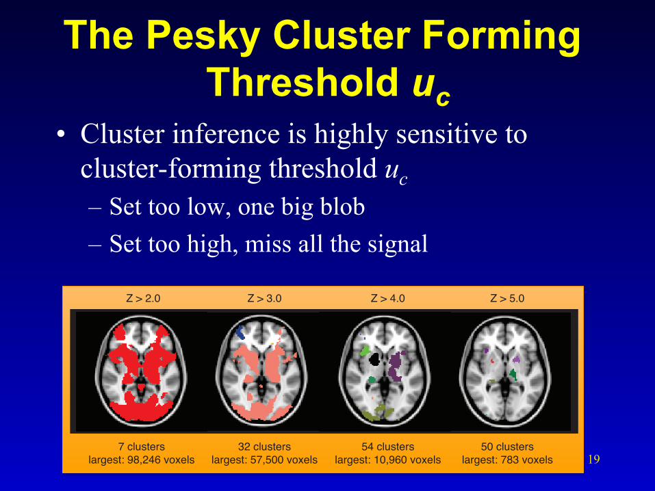
The Pesky Cluster Forming Threshold uc

•  Cluster inference is highly sensitive to cluster-forming threshold uc – Set too low, one big blob – Set too high, miss all the signal

19

Z > 2.0 Z > 3.0 Z > 4.0 Z > 5.0

7 clusterslargest: 98,246 voxels



50 clusterslargest: 783 voxels

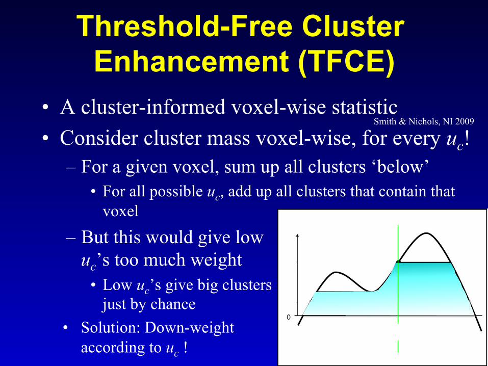
Threshold-Free Cluster Enhancement (TFCE)

•  A cluster-informed voxel-wise statistic

•  Consider cluster mass voxel-wise, for every uc! – For a given voxel, sum up all clusters ‘below’

•  For all possible uc, add up all clusters that contain that voxel

– But this would give low uc’s too much weight

•  Low uc’s give big clusters just by chance

20

Smith & Nichols, NI 2009


•  A cluster-informed voxel-wise statistic

•  Consider cluster mass voxel-wise, for every uc! – For a given voxel, sum up all clusters ‘below’

•  For all possible uc, add up all clusters that contain that voxel

– But this would give low uc’s too much weight

•  Low uc’s give big clusters just by chance

•  Solution: Down-weight according to uc !

Smith & Nichols, NI 2009

21

22


•  TFCE Statistic for voxel v

•  Parameters H & E control balance between cluster & height information – H=2 & E=1/2 as

motivated by theory

TFCE(v) =

∫ t(v)

0hHe(h)Edh ≈

∑0,δ,2δ,...,t(v)

hHe(h)Eδ

t(v)

Voxel v

e(h)

TFCE Redux •  Avoids choice of cluster-forming threshold uc

•  Generally more sensitive than cluster-wise •  But yet less specific

–  Inference is on some cluster for some uc

–  “Support” of effect could extend far from significant voxels

•  Implementation – Currently only

FSL’s randomise 23

24

Multiple comparisons…

25

Multiple Comparisons Problem

•  Which of 100,000 voxels are sig.? – α=0.05 ⇒ 5,000 false positive voxels

•  Which of (random number, say) 100 clusters significant? – α=0.05 ⇒ 5 false positives clusters

t > 0.5 t > 1.5 t > 2.5 t > 3.5 t > 4.5 t > 5.5 t > 6.5

26

MCP Solutions: Measuring False Positives

•  Familywise Error Rate (FWER) – Familywise Error

•  Existence of one or more false positives

– FWER is probability of familywise error •  False Discovery Rate (FDR)

– FDR = E(V/R) – R voxels declared active, V falsely so

•  Realized false discovery rate: V/R

27

Random field theory…

28

FWER MCP Solutions: Random Field Theory

•  Euler Characteristic χu – Topological Measure

•  #blobs - #holes

– At high thresholds, just counts blobs

– FWER = P(Max voxel ≥ u | Ho) = P(One or more blobs | Ho) ≈ P(χu ≥ 1 | Ho) ≈ E(χu | Ho)

Random Field

Suprathreshold Sets

Threshold

No holes

Never more than 1 blob

29

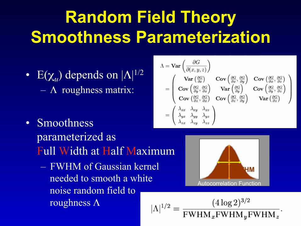
Random Field Theory Smoothness Parameterization

•  E(χu) depends on |Λ|1/2

–  Λ roughness matrix:

•  Smoothness parameterized as Full Width at Half Maximum –  FWHM of Gaussian kernel

needed to smooth a white noise random field to roughness Λ

Autocorrelation Function

FWHM

30

•  RESELS –  Resolution Elements –  1 RESEL = FWHMx × FWHMy × FWHMz –  RESEL Count R

•  R = λ(Ω) √ |Λ| = (4log2)3/2 λ(Ω) / ( FWHMx × FWHMy × FWHMz ) •  Volume of search region in units of smoothness •  Eg: 10 voxels, 2.5 FWHM 4 RESELS

•  Beware RESEL misinterpretation –  RESEL are not “number of independent ‘things’ in the image”

•  See Nichols & Hayasaka, 2003, Stat. Meth. in Med. Res. .

Random Field Theory Smoothness Parameterization

1 2 3 4

2 4 6 8 10 1 3 5 7 9

31

ε= β +Y X

data matrix

desi

gn m

atri

x

parameters errors+ ?= × ?voxelsvoxels

scansscans

estimate

β̂

residuals

estimatedcomponent

fields

parameterestimates

variance σ2

estimated variance

÷=

Random Field Theory Smoothness Estimation

•  Smoothness est’d from standardized residuals – Variance of

gradients – Yields resels per

voxel (RPV) •  RPV image

– Local roughness est. – Can transform in to local smoothness est.

•  FWHM Img = (RPV Img)-1/D

•  Dimension D, e.g. D=2 or 3 •  Est. smoothness also needed for AlphaSim

spm_imcalc_ui('RPV.img', ...!'FWHM.img','i1.^(-1/3)')!

32

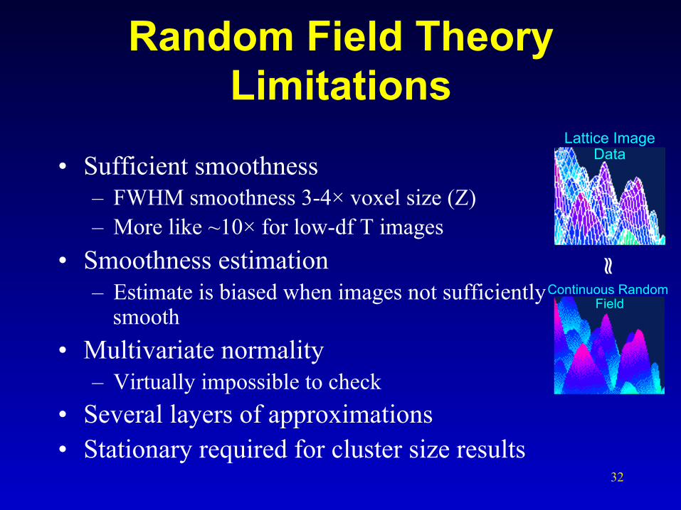
Random Field Theory Limitations

•  Sufficient smoothness –  FWHM smoothness 3-4× voxel size (Z) –  More like ~10× for low-df T images

•  Smoothness estimation –  Estimate is biased when images not sufficiently

smooth •  Multivariate normality

–  Virtually impossible to check •  Several layers of approximations •  Stationary required for cluster size results

Lattice Image Data

≈

Continuous Random Field

33

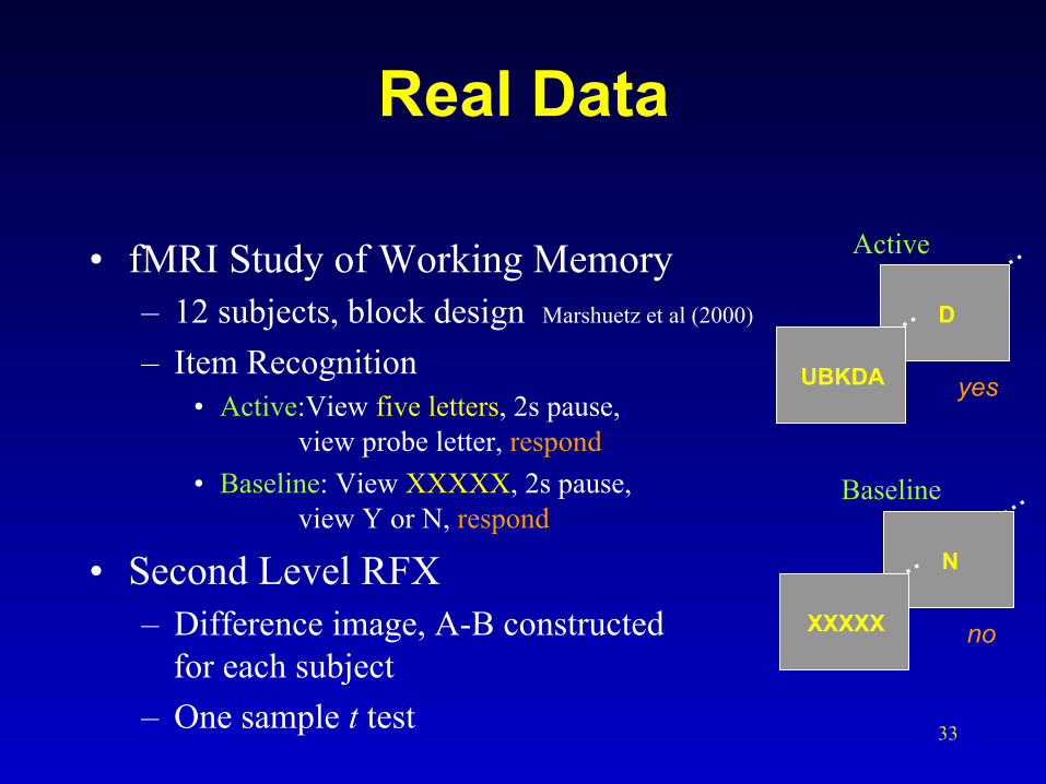
Real Data

•  fMRI Study of Working Memory –  12 subjects, block design Marshuetz et al (2000) –  Item Recognition

•  Active:View five letters, 2s pause, view probe letter, respond

•  Baseline: View XXXXX, 2s pause, view Y or N, respond

•  Second Level RFX –  Difference image, A-B constructed

for each subject –  One sample t test

D

yes UBKDA

Active

N

no XXXXX

Baseline

34

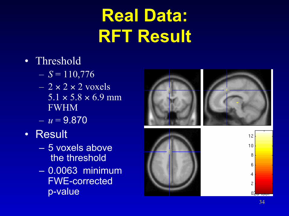
Real Data: RFT Result

•  Threshold –  S = 110,776 –  2 × 2 × 2 voxels

5.1 × 5.8 × 6.9 mm FWHM

–  u = 9.870 •  Result

–  5 voxels above the threshold

–  0.0063 minimum FWE-corrected p-value

-log 1

0 p-v

alue

35

Permutation…

Nonparametric Permutation Test

•  Parametric methods – Assume distribution of

statistic under null hypothesis

•  Nonparametric methods – Use data to find

distribution of statistic under null hypothesis

– Any statistic!

5%

Parametric Null Distribution

5%

Nonparametric Null Distribution

Permutation Test & Exchangeability

•  Exchangeability is fundamental –  Def: Distribution of the data unperturbed by

permutation –  Under H0, exchangeability justifies permuting data –  Allows us to build permutation distribution

•  fMRI scans not exchangeable over time! –  Even if no signal, autocorrelation structures data

•  Subjects are exchangeable –  Under Ho, each subject’s “active” “control” labels can

be flipped –  Equivalently, under Ho flip the sign of each subject’s

contrast images

Controlling FWE: Permutation Test

•  Parametric methods – Assume distribution of

max statistic under null hypothesis

•  Nonparametric methods – Use data to find

distribution of max statistic under null hypothesis

– Again, any max statistic!

5%

Parametric Null Max Distribution

5%

Nonparametric Null Max Distribution

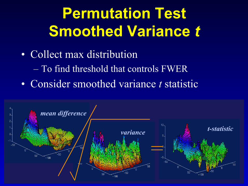
Permutation Test Smoothed Variance t

•  Collect max distribution – To find threshold that controls FWER

•  Consider smoothed variance t statistic

t-statistic variance

mean difference

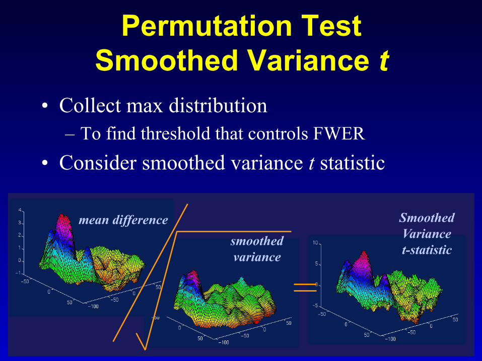
Permutation Test Smoothed Variance t

•  Collect max distribution – To find threshold that controls FWER

•  Consider smoothed variance t statistic

Smoothed Variance t-statistic

mean difference smoothed variance

Permutation Test Example

•  Permute! –  212 = 4,096 ways to flip 12 A/B labels – For each, note maximum of t image .

Permutation Distribution Maximum t

Orthogonal Slice Overlay Thresholded t

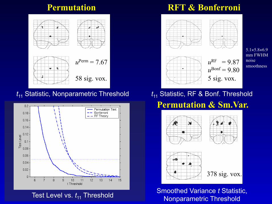
t11 Statistic, RF & Bonf. Threshold t11 Statistic, Nonparametric Threshold

uRF = 9.87 uBonf = 9.80 5 sig. vox.

uPerm = 7.67 58 sig. vox.

Smoothed Variance t Statistic, Nonparametric Threshold

378 sig. vox.

Test Level vs. t11 Threshold

5.1×5.8×6.9 mm FWHM noise smoothness

RFT & Bonferroni Permutation

Permutation & Sm.Var.

Reliability with Small Groups

•  Consider n=50 group study – Event-related Odd-Ball paradigm, Kiehl, et al.

•  Analyze all 50 – Analyze with SPM and SnPM, find FWE thresh.

•  Randomly partition into 5 groups 10 – Analyze each with SPM & SnPM, find FWE

thresh •  Compare reliability of small groups with full

– With and without variance smoothing .

SPM t11: 5 groups of 10 vs all 50 5% FWE Threshold

10 subj 10 subj 10 subj

10 subj 10 subj all 50

T>10.93 T>11.04 T>11.01

T>10.69 T>10.10 T>4.66

2 8 11 15 18 35 41 43 44 50 1 3 20 23 24 27 28 32 34 40 9 13 14 16 19 21 25 29 30 45

4 5 10 22 31 33 36 39 42 47 6 7 12 17 26 37 38 46 48 49

T>4.09

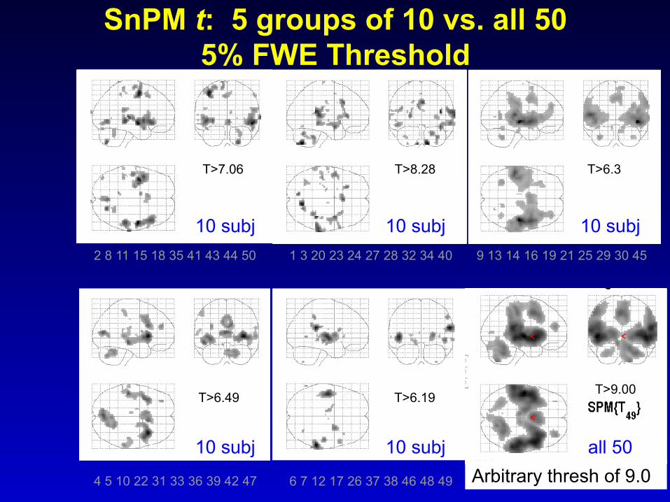
SnPM t: 5 groups of 10 vs. all 50 5% FWE Threshold


10 subj 10 subj

T>7.06 T>8.28 T>6.3

T>6.49 T>6.19

Arbitrary thresh of 9.0

T>9.00

all 50

2 8 11 15 18 35 41 43 44 50 1 3 20 23 24 27 28 32 34 40 9 13 14 16 19 21 25 29 30 45

4 5 10 22 31 33 36 39 42 47 6 7 12 17 26 37 38 46 48 49


10 subj 10 subj Arbitrary thresh of 9.0

T>9.00

all 50

SnPM SmVar t: 5 groups of 10 vs. all 50 5% FWE Threshold

T>4.69 T>5.04 T>4.57

T>4.84 T>4.64

2 8 11 15 18 35 41 43 44 50 1 3 20 23 24 27 28 32 34 40 9 13 14 16 19 21 25 29 30 45

4 5 10 22 31 33 36 39 42 47 6 7 12 17 26 37 38 46 48 49

47

False Discovery Rate…

48

MCP Solutions: Measuring False Positives

•  Familywise Error Rate (FWER) – Familywise Error

•  Existence of one or more false positives

– FWER is probability of familywise error •  False Discovery Rate (FDR)

– FDR = E(V/R) – R voxels declared active, V falsely so

•  Realized false discovery rate: V/R

49

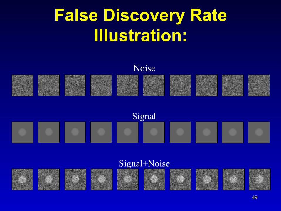
False Discovery Rate Illustration:

Signal

Signal+Noise

Noise

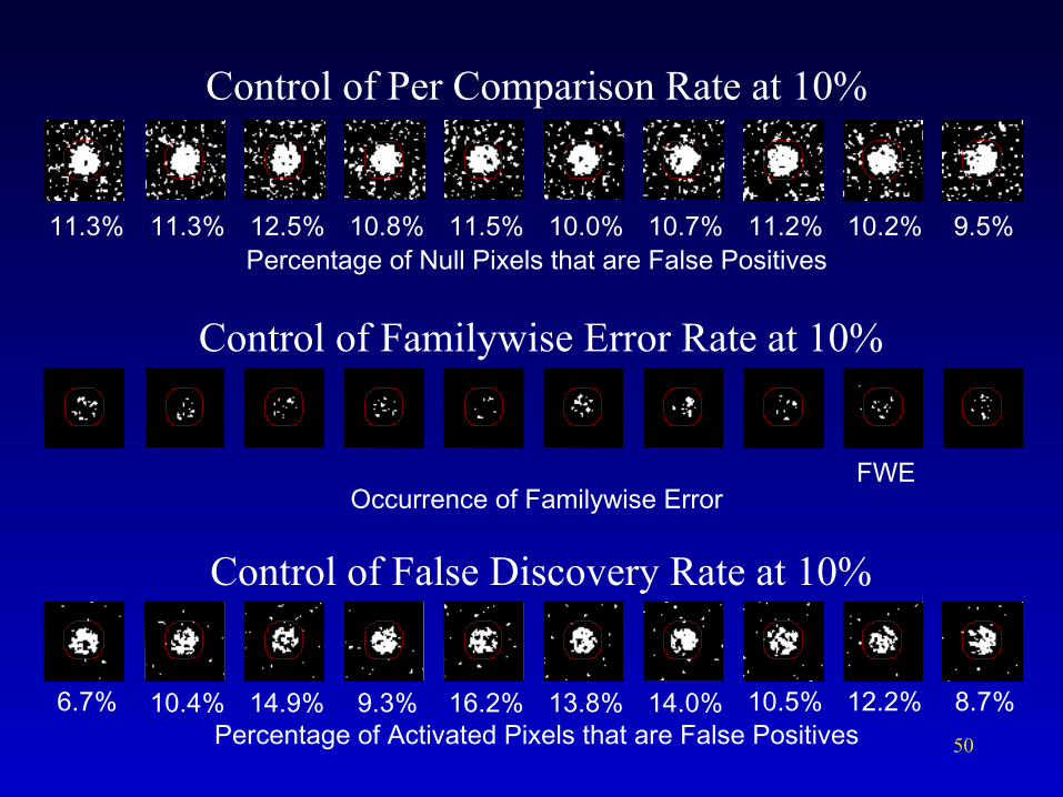
50

FWE

6.7% 10.4% 14.9% 9.3% 16.2% 13.8% 14.0% 10.5% 12.2% 8.7%

Control of Familywise Error Rate at 10%

11.3% 11.3% 12.5% 10.8% 11.5% 10.0% 10.7% 11.2% 10.2% 9.5%

Control of Per Comparison Rate at 10%

Percentage of Null Pixels that are False Positives

Control of False Discovery Rate at 10%

Occurrence of Familywise Error

Percentage of Activated Pixels that are False Positives

51

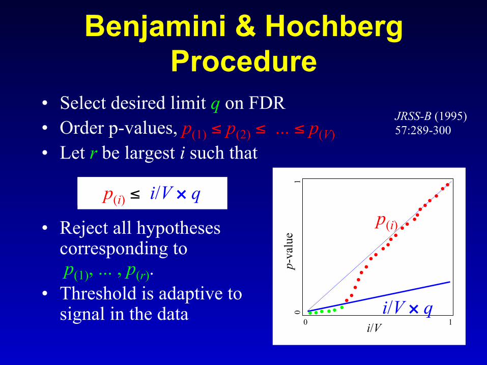
Benjamini & Hochberg Procedure

•  Select desired limit q on FDR •  Order p-values, p(1) ≤ p(2) ≤ ... ≤ p(V) •  Let r be largest i such that

•  Reject all hypotheses corresponding to p(1), ... , p(r).

•  Threshold is adaptive to signal in the data

p(i) ≤ i/V × q p(i)

i/V i/V × q

p-va

lue

0 1

0 1

JRSS-B (1995) 57:289-300

52 FWER Perm. Thresh. = 9.87 7 voxels

Real Data: FDR Example

FDR Threshold = 3.83 3,073 voxels

•  Threshold –  Indep/PosDep

u = 3.83 – Arb Cov

u = 13.15 •  Result

–  3,073 voxels above Indep/PosDep u

– <0.0001 minimum FDR-corrected p-value

53

Changes in SPM Inference

•  SPM 8 placed new emphasis on peak inference, removed voxel-wise FDR – FWE Voxel-wise & Peak-wise equivalent – FDR Voxel-wise & Peak-wise not equivalent!

•  To get voxel FDR, edit spm_defaults.m or do global defaults; defaults.stats.topoFDR=0;!

< SPM8 Uncorrected FDR FWE Voxel-wise × × × Cluster-wise × ×

≥ SPM8 Uncorrected FDR FWE Voxel-wise × Cluster-wise × × × Peak-wise × ×

Before SPM8

SPM8

54

Cluster FDR: Example Data Level 5% Cluster-FDR

P = 0.01 cluster-forming thresh kFDR = 1132, 4 clusters

Level 5% Cluster-FWE P = 0.01 cluster-forming thresh kFWE = 1132, 4 clusters 5 clusters

Level 5% Cluster-FDR, P = 0.001 cluster-forming thresh kFDR = 138, 6 clusters

Level 5% Cluster-FWE P = 0.001 cluster-forming thresh kFWE = 241, 5 clusters

Level 5% Voxel-FDR

Level 5% Voxel-FWE

55

Conclusions

•  Thresholding is not modeling! –  Just inference on a feature of a statistic image

•  Many features to choose from – Voxel-wise, cluster-wise, peak-wise…

•  FWER – Very specific, not very sensitive

•  FDR – Voxel-wise: Less specific, more sensitive – Cluster-, Peak-wise: Similar to FWER

56

References •  TE Nichols & S Hayasaka, Controlling the Familywise

Error Rate in Functional Neuroimaging: A Comparative Review. Statistical Methods in Medical Research, 12(5): 419-446, 2003.

TE Nichols & AP Holmes, Nonparametric Permutation Tests for Functional Neuroimaging: A Primer with Examples. Human Brain Mapping, 15:1-25, 2001.

CR Genovese, N Lazar & TE Nichols, Thresholding of Statistical Maps in Functional Neuroimaging Using the False Discovery Rate. NeuroImage, 15:870-878, 2002.

JR Chumbley & KJ Friston. False discovery rate revisited: FDR and topological inference using Gaussian random fields. NeuroImage, 44(1), 62-70, 2009

new and best-practice approaches to thresholding

Documents