new analysis of adaptive stochastic optimization methods ... · introduction and motivation outline...
TRANSCRIPT

New Analysis of Adaptive Stochastic OptimizationMethods via Martingales.
Katya Scheinbergjoint work with J. Blanchet (Stanford), C. Cartis (Oxford), M. Menickelly (Argonne) and C.
Paquette (Waterloo)
Princeton Day of Optimization
September 28, 2018
Katya Scheinberg (Lehigh) Stochastic Framework September 28, 2018 1 / 35

Outline
1 Introduction and Motivation
2 Stochastic Trust Region and Line Search Methods
3 A Supermatringale and its Stopping Time
4 Convergence Rate for Stochastic Methods
Katya Scheinberg (Lehigh) Stochastic Framework September 28, 2018 2 / 35

Introduction and Motivation
Outline
1 Introduction and Motivation
2 Stochastic Trust Region and Line Search Methods
3 A Supermatringale and its Stopping Time
4 Convergence Rate for Stochastic Methods
Katya Scheinberg (Lehigh) Stochastic Framework September 28, 2018 3 / 35

Introduction and Motivation
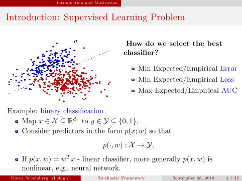
Introduction: Supervised Learning Problem
How do we select the bestclassifier?
Min Expected/Empirical Error
Min Expected/Empirical Loss
Max Expected/Empirical AUC
Example: binary classification
Map x ∈ X ⊆ Rdx to y ∈ Y ⊆ {0, 1}.Consider predictors in the form p(x;w) so that
p(·, w) : X → Y,
If p(x,w) = wTx - linear classifier, more generally p(x,w) isnonlinear, e.g., neural network.
Katya Scheinberg (Lehigh) Stochastic Framework September 28, 2018 4 / 35
Introduction and Motivation
Introduction: Supervised Learning Problem
How do we select the bestclassifier?
Min Expected/Empirical Error
Min Expected/Empirical Loss
Max Expected/Empirical AUC
Example: binary classification
Map x ∈ X ⊆ Rdx to y ∈ Y ⊆ {0, 1}.Consider predictors in the form p(x;w) so that
p(·, w) : X → Y,
If p(x,w) = wTx - linear classifier, more generally p(x,w) isnonlinear, e.g., neural network.
Katya Scheinberg (Lehigh) Stochastic Framework September 28, 2018 4 / 35

Introduction and Motivation
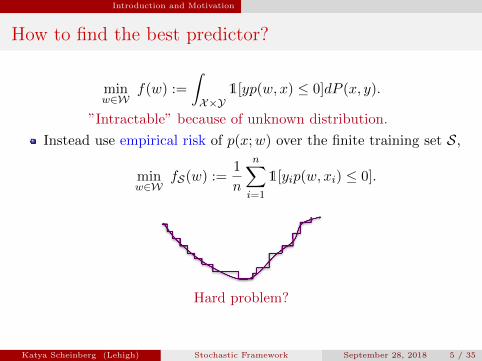
How to find the best predictor?
minw∈W
f(w) :=
∫X×Y
1[yp(w, x) ≤ 0]dP (x, y).
”Intractable” because of unknown distribution.
Instead use empirical risk of p(x;w) over the finite training set S,
minw∈W
fS(w) :=1
n
n∑i=1
1[yip(w, xi) ≤ 0].
Instead use ”smooth” or ”easy” empirical loss p(x;w) over thefinite training set S,
minw∈W
f̂`(w) :=1
n
n∑i=1
`(p(w, xi), yi).
This is a tractable problem but n and dw can be large!!
Katya Scheinberg (Lehigh) Stochastic Framework September 28, 2018 5 / 35
Introduction and Motivation
How to find the best predictor?
minw∈W
f(w) :=
∫X×Y
1[yp(w, x) ≤ 0]dP (x, y).
”Intractable” because of unknown distribution.
Instead use empirical risk of p(x;w) over the finite training set S,
minw∈W
fS(w) :=1
n
n∑i=1
1[yip(w, xi) ≤ 0].
Hard problem?
Instead use ”smooth” or ”easy” empirical loss p(x;w) over thefinite training set S,
minw∈W
f̂`(w) :=1
n
n∑i=1
`(p(w, xi), yi).
This is a tractable problem but n and dw can be large!!
Katya Scheinberg (Lehigh) Stochastic Framework September 28, 2018 5 / 35

Introduction and Motivation
How to find the best predictor?
minw∈W
f(w) :=
∫X×Y
1[yp(w, x) ≤ 0]dP (x, y).
”Intractable” because of unknown distribution.
Instead use empirical risk of p(x;w) over the finite training set S,
minw∈W
fS(w) :=1
n
n∑i=1
1[yip(w, xi) ≤ 0].
Instead use ”smooth” or ”easy” empirical loss p(x;w) over thefinite training set S,
minw∈W
f̂`(w) :=1
n
n∑i=1
`(p(w, xi), yi).
This is a tractable problem but n and dw can be large!!
Katya Scheinberg (Lehigh) Stochastic Framework September 28, 2018 5 / 35

Introduction and Motivation
What’s been happening in optimization under theinfluence of machine learning applications?
”New” scale - optimizing very large sums
Stochasticity - optimizing averages and/or expectations
Inexactness - optimizing using ”cheap” inexact steps
Complexity - emphasis on complexity bounds
Katya Scheinberg (Lehigh) Stochastic Framework September 28, 2018 6 / 35
Introduction and Motivation
Stochastic Optimization Setting
Minimize f(x) : Rn → R
We will assume throughout that f is L-smooth and boundedbelow.
f is nonconvex unless specified.
f(x) is stochastic, i.e. given x, we obtain estimates f̃(x, ξ), (andpossibly ∇f̃(x, ξ)), where ξ is a random variable.
Note: f(x) and ∇f(x) are not necessarily equal to Eξ[f̃(x, ξ)],Eξ[∇f̃(x, ξ)]
Katya Scheinberg (Lehigh) Stochastic Framework September 28, 2018 7 / 35

Introduction and Motivation
Motivation #1: Adaptive Methods
Standard stochastic gradient method
Assume Eξ[∇f̃(xk, ξ)] = ∇f(xk) for all xk.
Generate ξ1, ξ2, . . . , ξsk using a predefined sample (mini-batch) sizesk and compute
∇skf(x) =1
sk
sk∑i=1
∇f̃(xk, ξi).
Take a step xk+1 = xk − αk∇skf(x) with predefined step size αk(learning rate).
In deterministic optimization adaptive methods are more efficient!
Can we design and analyze adaptive stochastic methods?
Katya Scheinberg (Lehigh) Stochastic Framework September 28, 2018 8 / 35

Introduction and Motivation
Motivation #1: Adaptive Methods
Standard stochastic gradient method
Assume Eξ[∇f̃(xk, ξ)] = ∇f(xk) for all xk.
Generate ξ1, ξ2, . . . , ξsk using a predefined sample (mini-batch) sizesk and compute
∇skf(x) =1
sk
sk∑i=1
∇f̃(xk, ξi).
Take a step xk+1 = xk − αk∇skf(x) with predefined step size αk(learning rate).
In deterministic optimization adaptive methods are more efficient!
Can we design and analyze adaptive stochastic methods?Katya Scheinberg (Lehigh) Stochastic Framework September 28, 2018 8 / 35

Introduction and Motivation
(Deterministic) Backtracking Line Search
Backtracking Line Search Algorithm
Choose initial point x0, initial step-size α0 ∈ (0, αmax) withαmax > 0. Choose constant γ > 1, set k ← 0.
For k = 0, 1, 2, . . .
Compute a descent direction −gk.Compute f(xk) and f(xk − αkgk) and check sufficient decrease:
f(xk − αkgk) ≤ f(xk)− θαk‖gk‖2.
Successful: xk+1 = xk − αk∇f(xk) and αk+1 = min{γαk, αmax}.Unsuccessful: xk+1 = xk and αk+1 = αk/γ.
Katya Scheinberg (Lehigh) Stochastic Framework September 28, 2018 9 / 35

Introduction and Motivation
(Deterministic) Trust Region Method
Choose initial point x0, initial trust-region radius δ0 ∈ (0, δmax) with δmax > 0.Choose constants γ > 1, η1 ∈ (0, 1), η2 > 0. Set k ← 0.
For k = 0, 1, 2, . . .
Build a local model mk(·) of f on B(0, δk).
Compute sk = arg mins:‖s‖≤δk
mk(s) (approximately).
Compute ρk =f(xk)− f(xk + sk)
mk(xk)−mk(xk + sk).
If ρk ≥ η1 and ‖∇mk(xk)‖ ≥ η2δk then xk+1 = xk + sk (Successful)else xk+1 = xk (Unsuccessful).
If successful then δk+1 = min{γδk, δmax}If unsuccessful then δk+1 = γ−1δk.
Katya Scheinberg (Lehigh) Stochastic Framework September 28, 2018 10 / 35

Introduction and Motivation
Complexity Bounds
Deterministic Line Search and Trust Region
‖∇f(xk)‖ < ε f(xk)− f∗ < ε
L-smooth Lε2
-
L-smooth/convex Lε2
Lε
µ-strongly convex Lµ · log(1
ε ) Lµ · log(1
ε )
Stochastic Gradient
‖∇f(xk)‖ < ε f(xk)− f∗ < ε
L-smooth Lε4
-
L-smooth/convex Lε4
Lε2
µ-strongly convex Lε2
Lε
Katya Scheinberg (Lehigh) Stochastic Framework September 28, 2018 11 / 35

Introduction and Motivation
Motivation #2: Recovering Deterministic Complexity
Various adaptive stochastic methods that havepartial convergence rates results matching deterministic rates.
Friedlander and Schmidt. ”Hybrid deterministic-stochastic methods for datafitting”. SIAM Journal on Scientific Computing 34(3), 2012.Convergence rate for strongly convex case based on exponentially increasingsample size.
Hashemi, Ghosh, and Pasupathy. ”On adaptive sampling rules for stochasticrecursions”. Simulation Conference (WSC), IEEE, 2014.No rates, convergence with probability one by increasing sample sizeindefinitely.
Bollapragada, Byrd, and Nocedal. ”Adaptive sampling strategies for stochasticoptimization”. arXiv:1710.11258, 2017.Good heuristic ideas, convergence rates only when sample size chosen based onthe true gradient.
Katya Scheinberg (Lehigh) Stochastic Framework September 28, 2018 12 / 35

Introduction and Motivation
Motivation #2: Recovering Deterministic Complexity
Various adaptive stochastic methods that havepartial convergence rates results matching deterministic rates.
Roosta-Khorasani and Mahoney. ”Sub-sampled newton methods I: Globallyconvergent algorithms”. arXiv:1601.04737, 2017Only Hessian estimates are stochastic, fixed large sample size, complexitybound established only under assumption that estimates are accurate at eachiteration.
Tripuraneni, Stern, Jin, Regier, and Jordan. ”Stochastic cubic regularizationfor fast nonconvex optimization”. arXiv:1711.02838, 2017Fixed large sample sizes, fixed small step size, complexity bound establishedonly under assumption that estimates are accurate at each iteration.
Full convergence rates results are needed
Katya Scheinberg (Lehigh) Stochastic Framework September 28, 2018 12 / 35

Introduction and Motivation
Motivation #3: Expected Convergence Rate vs.Expected Complexity
Complexity bound in deterministic optimization is the bound on the firstiteration Tε that achieves ε-accuracy, e.g. for nonconvex f
‖∇f(xk)‖ ≤ ε⇒ Tε ≤ O(1
ε2)
Then convergence rate is
‖∇f(xk)‖2 ≤ O(1
T)
Convergence rate for stochastic algorithms for nonconvex f is the expectedaccuracy at the output xT (usually random) produced after first T iterations
E[‖∇f(xT )‖2] ≤ 1√T
In some cases bound on Tε is only derived with high probability.
Can we bound E[Tε]?
Katya Scheinberg (Lehigh) Stochastic Framework September 28, 2018 13 / 35
Introduction and Motivation
Prior works that bound E[Tε]
Cartis and Scheinberg. ”Global convergence rate analysis of unconstrainedoptimization methods based on probabilistic models”. MathematicalProgramming 2017.First-order rates for line-search in nonconvex, convex and strongly convexcases, adaptive cubic regularization for nonconvex case.
Gratton, Royer, Vicente, and Zhang. ”Complexity and global rates oftrust-region methods based on probabilistic models”, IMA Journal ofNumerical Analysis, 2018.First- and second-order rates for trust region in the nonconvex case.
Only Hessian and gradient estimates are stochastic
Katya Scheinberg (Lehigh) Stochastic Framework September 28, 2018 14 / 35

Introduction and Motivation
Motivation #4: Biased Estimates
Consider example:
f(x) =
n∑i=1
(xi − 1)2
f̃(x, ξ) =
n∑i=1
wi, where wi =
{(xi − 1)2 w.p. p−10000 w.p. 1− p
For p < 1, this noise is biased (Eξ[f̃(x, ξ)] 6= f(x)).
Does not fit into the assumptions of standard algorithms andanalysis.
Can we have convergence if p is sufficiently large?
Katya Scheinberg (Lehigh) Stochastic Framework September 28, 2018 15 / 35

Stochastic Trust Region and Line Search Methods
Outline
1 Introduction and Motivation
2 Stochastic Trust Region and Line Search Methods
3 A Supermatringale and its Stopping Time
4 Convergence Rate for Stochastic Methods
Katya Scheinberg (Lehigh) Stochastic Framework September 28, 2018 16 / 35

Stochastic Trust Region and Line Search Methods
Stochastic Trust Region Method
Choose initial point x0, initial trust-region radius δ0 ∈ (0, δmax) with δmax > 0.Choose constants γ > 1, η1 ∈ (0, 1), η2 > 0. Set k ← 0.
For k = 0, 1, 2, . . .
Build a local random model mk(·) of f on B(0, δk).
Compute sk = arg mins:‖s‖≤δk
mk(s) (approximately).
Compute ρk =f(xk)− f(xk + sk)
mk(xk)−mk(xk + sk).
If ρk ≥ η1 and ‖∇mk(xk)‖ ≥ η2δk then xk+1 = xk + sk (Successful)else xk+1 = xk (Unsuccessful).
If successful then δk ↑If unsuccessful then δk ↓
Katya Scheinberg (Lehigh) Stochastic Framework September 28, 2018 17 / 35

Stochastic Trust Region and Line Search Methods
What can happen?
Katya Scheinberg (Lehigh) Stochastic Framework September 28, 2018 18 / 35

Stochastic Trust Region and Line Search Methods
What else can happen
Katya Scheinberg (Lehigh) Stochastic Framework September 28, 2018 19 / 35

Stochastic Trust Region and Line Search Methods
Stochastic Line Search
Compute random estimate of the gradient, gk
Compute random estimates f0k ≈ f(xk) and fsk ≈ f(xk − αkgk)
Check the sufficient decrease
fsk ≤ f0k − θαk ‖gk‖
2
Successful: xk+1 = xk − αkgk and αk ↑
Reliable step: If αk ‖gk‖2 ≥ δ2k, δk ↑Unreliable step: If αk ‖gk‖2 < δ2k, δk ↓
Unsucessful: xk+1 = xk, αk ↓, and δk ↓
Katya Scheinberg (Lehigh) Stochastic Framework September 28, 2018 20 / 35

A Supermatringale and its Stopping Time
Outline
1 Introduction and Motivation
2 Stochastic Trust Region and Line Search Methods
3 A Supermatringale and its Stopping Time
4 Convergence Rate for Stochastic Methods
Katya Scheinberg (Lehigh) Stochastic Framework September 28, 2018 21 / 35

A Supermatringale and its Stopping Time
Stochastic Process (Algorithm)
Consider a stochastic process {Φk,∆k} ≥ 0 and its stopping time Tε.Intuitively:
Φk is progress towards optimality (order of f(xk)− fmin).
∆k is the step size parameter (trust region radius/learning rate).
Tε is the first iteration k to reach accuracy ε (‖∇f(Xk)‖ ≤ ε).
Katya Scheinberg (Lehigh) Stochastic Framework September 28, 2018 22 / 35

A Supermatringale and its Stopping Time
The ∆k Process
Key Assumption (i):There exists a constant ∆ε such that, until the stopping time:
∆k+1 ≥ min(γWk+1∆k,∆ε),
where Wk+1 is a random walk with positive drift (p > 12).
Katya Scheinberg (Lehigh) Stochastic Framework September 28, 2018 23 / 35

A Supermatringale and its Stopping Time
The ∆k Process
Key Assumption (ii):There exists a nondecreasing function h(·) : [0,∞)→ (0,∞) and aconstant Θ > 0 such that, until the stopping time:
E(Φk+1|Fk) ≤ Φk −Θh(∆k).
Katya Scheinberg (Lehigh) Stochastic Framework September 28, 2018 23 / 35

A Supermatringale and its Stopping Time
The ∆k Process
Main Idea:
∆k may get arbitrarily small, but it tends to return to ∆ε.
∆k is a birth-death process with known interarrival timesdepending p.
Count the returns of ∆k to ∆ε - a renewal cycle.
For each renewal the is a fixed expected reward.Katya Scheinberg (Lehigh) Stochastic Framework September 28, 2018 24 / 35

A Supermatringale and its Stopping Time
Bounding expected stopping time
Main Idea: This is a renewal-reward process and Φk is asupermartingale and Φ0 ≥ Θ
∑Tεi=0 h(∆i).
Tε is a stopping time!
Applying Wald’s Identity we can bound the number of renewalsthat will occur before Tε.
Multiply by the expected renewal time.
We have the following results
Theorem (Blanchet, Cartis, Menickelly, S. ’17)
Let the Key Assumption hold. Then
E[Tε] ≤p
2p− 1· Φ0
Θh(∆ε)+ 1.
Katya Scheinberg (Lehigh) Stochastic Framework September 28, 2018 25 / 35

Convergence Rate for Stochastic Methods
Outline
1 Introduction and Motivation
2 Stochastic Trust Region and Line Search Methods
3 A Supermatringale and its Stopping Time
4 Convergence Rate for Stochastic Methods
Katya Scheinberg (Lehigh) Stochastic Framework September 28, 2018 26 / 35

Convergence Rate for Stochastic Methods
Assumptions on models and estimates
For trust region, first-order
‖∇f(xk)−∇mk(xk)‖ ≤ O(δk), w.p. pg
|f0k − f(xk)| ≤ O(δ2
k) and |fsk − f(xk + sk)| ≤ O(δ2k). w.p. pf
For trust region, second-order
‖∇2f(xk)−∇2mk(xk)‖ ≤ O(δk)
‖∇f(xk)−∇mk(xk)‖ ≤ O(δ2
k), w.p. pg
|f0k − f(xk)| ≤ O(δ2
k) and |fsk − f(xk + sk)| ≤ O(δ3k). w.p. pf
p = pf ∗ pg
Katya Scheinberg (Lehigh) Stochastic Framework September 28, 2018 27 / 35

Convergence Rate for Stochastic Methods
Assumptions on models and estimates
For line search
‖∇f(xk)− gk‖ ≤ O(αk‖gk‖), w.p. pg
|f0k − f(xk)| ≤ O(δ2
k) and |fsk − f(xk + sk)| ≤ O(δ2k). w.p. pf
E|f0k − f(xk)| ≤ O(δ2
k)
p = pf ∗ pg
Katya Scheinberg (Lehigh) Stochastic Framework September 28, 2018 27 / 35

Convergence Rate for Stochastic Methods
Stochastic TR: First-order convergence rate.
∆k is the trust region radius.
Φk = ν(f(xk)− fmin) + (1− ν)∆2k.
Tε = inf{k ≥ 0 : ‖∇f(Xk)‖ ≤ ε}.
Theorem
(Blanchet-Cartis-Menickelly-S. ’17)
E[Tε] ≤ O(
p
2p− 1
(L
ε2
)),
Katya Scheinberg (Lehigh) Stochastic Framework September 28, 2018 28 / 35

Convergence Rate for Stochastic Methods
Stochastic TR: Second-order convergence rate
∆k is the trust region radius.
Φk = ν(f(xk)− fmin) + (1− ν)∆2k.
Tε = inf{k ≥ 0 : max{‖∇f(Xk)‖,−λmin(∇2f(Xk))} ≤ ε}.
Theorem
(Blanchet-Cartis-Menickelly-S. ’17)
E[Tε] ≤ O(
p
2p− 1
(L
ε3
)),
Katya Scheinberg (Lehigh) Stochastic Framework September 28, 2018 29 / 35

Convergence Rate for Stochastic Methods
Stochastic line search: nonconvex case
∆k = αk - the step size parameter.
Φk = ν(f(xk)− fmin) + (1− ν)αk ‖∇f(xk)‖2 + (1− ν)θδ2k.
Tε = inf{k ≥ 0 : ‖∇f(Xk)‖ ≤ ε}.
Theorem
(Paquette-S. ’18)
E[Tε] ≤ O(
p
2p− 1
(L3
ε2
)),
Katya Scheinberg (Lehigh) Stochastic Framework September 28, 2018 30 / 35

Convergence Rate for Stochastic Methods
Stochastic line search: convex case
∆k = αk - the step size parameter.
Φk = ν(f(xk)− fmin) + (1− ν)αk ‖∇f(xk)‖2 + (1− ν)θδ2k.
Tε = inf{k : f(xk)− f∗ < ε}.Ψk = 1
νε −1
Φk.
Theorem
(Paquette-S. ’18)
E[Tε] ≤ O(
p
2p− 1
(L3
ε
)),
Katya Scheinberg (Lehigh) Stochastic Framework September 28, 2018 31 / 35

Convergence Rate for Stochastic Methods
Stochastic line search: strongly convex case
∆k = αk - the step size parameter.
Φk = ν(f(xk)− fmin) + (1− ν)αk ‖∇f(xk)‖2 + (1− ν)θδ2k.
Tε = inf{k : f(xk)− f∗ < ε}.Ψk = log(Φk)− log(νε).
Theorem
(Paquette-S. ’18)
E[Tε] ≤ O(
p
2p− 1log
(L3
ε
)),
Katya Scheinberg (Lehigh) Stochastic Framework September 28, 2018 32 / 35

Convergence Rate for Stochastic Methods
Conclusions and Remarks
We have a powerful framework based on bounding stoping time ofa martingale which can be used to derive expected complexitybounds for adaptive stochastic methods.
Accuracy requirement of function value estimates are muchheavier than those for gradient estimates.
Accuracy requirement of gradient value estimates are somewhatheavier than those for gradient estimates.
Algorithms can converge even with constant probability of”iteration failure.”
Katya Scheinberg (Lehigh) Stochastic Framework September 28, 2018 33 / 35

Convergence Rate for Stochastic Methods
Depp Learning
The problem is not the problem. The problem isyour attitude about the problem
Jack Sparrow, Pirates of the Caribbean
Katya Scheinberg (Lehigh) Stochastic Framework September 28, 2018 34 / 35

Convergence Rate for Stochastic Methods
Thanks for listening!
J. Blanchet, C. Cartis, M. Menickelly, and K. Scheinberg, ”Convergence RateAnalysis of a Stochastic Trust Region Method via Submartingales”.arXiv:1609.07428, 2017.
C. Paquette, K. Scheinberg, ”A Stochastic Line Search Method withConvergence Rate Analysis”. arXiv:1807.07994, 2018.
Katya Scheinberg (Lehigh) Stochastic Framework September 28, 2018 35 / 35