neutronics modeling of the high flux isotope reactor using comsol

Annals of Nuclear Energy 38 (2011) 2594–2605

Contents lists available at ScienceDirect

Annals of Nuclear Energy

journal homepage: www.elsevier .com/locate /anucene

Neutronics modeling of the High Flux Isotope Reactor using COMSOL

David Chandler a,⇑, G. Ivan Maldonado a, R.T. Primm III b,1, J.D. Freels b

a University of Tennessee, Department of Nuclear Engineering, 311 Pasqua Engineering, Knoxville, TN 37996-2300, USAb Oak Ridge National Laboratory, Research Reactors Division, P.O. Box 2008, Oak Ridge, TN 37831-6399, USA

a r t i c l e i n f o

Article history:Received 21 February 2011Accepted 3 June 2011Available online 2 August 2011

Keywords:HFIRCOMSOL MultiphysicsDiffusion theoryNeutronicsSCALENEWT

0306-4549/$ - see front matter � 2011 Elsevier Ltd. Adoi:10.1016/j.anucene.2011.06.002

⇑ Corresponding author. Tel.: +1 865 974 7562; faxE-mail addresses: [email protected], chandlerd@or

[email protected] (G.I. Maldonado), trentprimm@[email protected] (J.D. Freels).

1 Present address: Primm Consulting, LLC, USA.

a b s t r a c t

The High Flux Isotope Reactor located at the Oak Ridge National Laboratory is a versatile 85 MWth researchreactor with cold and thermal neutron scattering, materials irradiation, isotope production, and neutronactivation analysis capabilities. HFIR staff members are currently in the process of updating the thermalhydraulic and reactor transient modeling methodologies. COMSOL Multiphysics has been adopted forthe thermal hydraulic analyses and has proven to be a powerful finite-element-based simulation tool forsolving multiple physics-based systems of partial and ordinary differential equations. Modeling reactortransients is a challenging task because of the coupling of neutronics, heat transfer, and hydrodynamics.This paper presents a preliminary COMSOL-based neutronics study performed by creating a two-dimen-sional, two-group, diffusion neutronics model of HFIR to study the spatially-dependent, beginning-of-cyclefast and thermal neutron fluxes. The 238-group ENDF/B-VII neutron cross section library and NEWT, a two-dimensional, discrete-ordinates neutron transport code within the SCALE 6 code package, were used to cal-culate the two-group neutron cross sections required to solve the diffusion equations. The two-group dif-fusion equations were implemented in the COMSOL coefficient form PDE application mode and were solvedvia eigenvalue analysis using a direct (PARDISO) linear system solver. A COMSOL-provided adaptive meshrefinement algorithm was used to increase the number of elements in areas of largest numerical error toincrease the accuracy of the solution. The flux distributions calculated by means of COMSOL/SCALE com-pare well with those calculated with benchmarked three-dimensional MCNP and KENO models, a necessaryfirst step along the path to implementing two- and three-dimensional models of HFIR in COMSOL for thepurpose of studying the spatial dependence of transient-induced behavior in the reactor core.

� 2011 Elsevier Ltd. All rights reserved.

1. Introduction

Neutron diffusion theory is one of the simplest and most widelyused methods to determine the neutron distribution within a reac-tor and can be used to characterize as many neutron energy groupsas the user desires (Stacey, 2001). The two-group, spatially-depen-dent neutron diffusion equations were implemented in COMSOLMultiphysics v3.5a (COMSOL, 2008) to simulate neutron transportin a two-dimensional model of the High Flux Isotope Reactor(HFIR) in order to determine the thermal and fast neutron distribu-tions within the reactor at steady-state beginning-of-cycle (BOC)conditions. This task was the first step to accomplishing atime-dependent neutronics solution in COMSOL using a two-dimensional and then a three-dimensional model of HFIR. The pur-pose of the model development is to study the spatial dependenceof transient-induced behavior in the reactor core. A COMSOL-based

ll rights reserved.

: +1 865 974 0668.nl.gov (D. Chandler), Ivan.Mal-onsultingllc.com (R.T. Primm),

thermal hydraulic and structural analysis model of the HFIR is un-der development in an independent but parallel project (Primm,2011). That model is expected to eventually be merged with thecurrent work to form a comprehensive multiphysics solution fortransient-induced behavior.

The cross sections needed to solve the diffusion equations werecalculated by means of NEWT (DeHart, 2009), a two-dimensionalneutron transport code in the SCALE 6 package (SCALE, 2009).The same geometry used in NEWT was created in COMSOL andthe cross sections calculated by NEWT were inserted into COMSOL.The diffusion equations and associated boundary conditions werecoded into COMSOL by means of the partial differential equation(PDE) coefficient application mode and the flux profiles in the HFIRcore were solved via eigenvalue analysis and a direct (PARDISO)linear system solver. A COMSOL-provided adaptive mesh refine-ment algorithm was used to solve the diffusion equations using asequence of refined meshes by increasing the number of elementsin areas where the previous calculation (same PDE problem, butdifferent mesh) yielded the largest numerical errors. Similar diffu-sion analyses have been performed for a molten salt breeder reac-tor (MSBR) core channel (Memoli et al., 2009) and a CANDU lattice(Gomes, 2008).

http://dx.doi.org/10.1016/j.anucene.2011.06.002

mailto:[email protected]



http://dx.doi.org/10.1016/j.anucene.2011.06.002

http://www.sciencedirect.com/science/journal/03064549

http://www.elsevier.com/locate/anucene

Fig. 2. Schematic representation of NEWT and COMSOL models.

D. Chandler et al. / Annals of Nuclear Energy 38 (2011) 2594–2605 2595

1.1. High Flux Isotope Reactor description

HFIR is a versatile research reactor located at the Oak Ridge Na-tional Laboratory (ORNL). HFIR was constructed in the mid-1960sfor the purpose of producing heavy (transuranic) isotopes like252Cf. Today, the steady-state neutron fluxes produced in this85 MWth reactor are utilized for cold and thermal neutron scatter-ing, materials irradiation, isotope production, and neutron activa-tion analysis.

HFIR is a pressurized, light water-cooled and -moderated reac-tor that was designed with an over-moderated flux-trap (FT) in thecenter of the core and a large beryllium reflector on the outside ofthe core in order to produce a large thermal flux to power ratio forthe purpose of transuranic isotope production. The central FT issurrounded by two concentric fuel annuli containing highly en-riched uranium (HEU) in aluminum clad and water coolant chan-nels. On the outside of the fuel elements (FE) are two concentricpoison bearing control elements (CE), a large beryllium reflector,and light water. A mockup of HFIR is presented in Fig. 1.

The FT consists of 37 target rod locations that accommodatematerials to be activated. The FE consists of an inner fuel element(IFE) and an outer fuel element (OFE), each constructed of alumi-num involute plates (171 in IFE and 369 in OFE) containing ura-nium enriched to approximately 93 weight percent in 235U/U inthe form of U3O8 in an aluminum matrix. The total loading of afresh HFIR core is about 9.4 kg of 235U and a typical fuel cyclelength ranges between 22 and 26 days depending on the experi-ment loading. The CEs are located between the fuel and the reflec-tor and each consist of three sections: a black region (Eu2O3–Al), agrey region (Ta–Al), and a white region (Al), and are named basedon their neutron absorbing capability.

1.2. Computer code description

NEWT is a multi-group discrete-ordinates code that is run with-in SCALE, a code package developed and maintained at ORNL.NEWT performs two-dimensional (2-D) neutron transport calcula-tions and utilizes the Extended Step Characteristic (ESC) approachfor spatial discretization on an arbitrary mesh structure. The pri-mary function of NEWT is to calculate the spatial flux distributionswithin a nuclear system and collapse the cross sections into multi-ple (or single) energy groups as specified by the user. Thesecollapsed cross sections can be supplied to ORIGEN-S for depletion

Fig. 1. Mockup of the High Flux Isotope Reactor.

calculations, or in the case of this study, can be extracted from theoutput for use in another application (DeHart, 2009).

COMSOL Multiphysics is a software package that uses the finiteelement method for spatial discretization to solve physics-basedsystems of PDEs and/or ODEs. Steady-state and time-dependentmultiphysics simulations can be set up using the predefined (i.e.built-in) physics/engineering modules or by specifying a systemof user-specific PDEs. Additional built-in modules can be modifiedto the user’s needs through equation based modeling capabilitiesand can be coupled together with other modules, with user definedPDEs, or with external coding through a MATLAB interface, all ofwhich makes COMSOL a versatile simulation tool.

2. NEWT model development

A two-dimensional NEWT model of HFIR was developed bymodifying an existing NEWT model of HFIR that was created forlow enriched uranium (LEU) conversion studies (Primm, 2009).The major modifications to the LEU model included changing thefuel to HEU, modeling the CEs in the control region, and by model-ing the bottom half of HFIR rather than using symmetry across thecore horizontal midplane (y = 0). The geometry utilized in the LEUmodel is a two-dimensional quarter configuration of HFIR suchthat symmetry was utilized at the core horizontal midplane andthe core vertical centerline (x = 0, cartesian geometry). The HEUmodel developed for these studies utilized the same radial and ax-ial boundaries and atomic densities as used in benchmarked three-dimensional HEU TRITON (Chandler and Primm, 2009) and MCNP(Primm, 2005) models. The HEU input models a half configurationof HFIR such that symmetry was only utilized across the core cen-terline (x = 0, cartesian geometry).

The flux trap is modeled as multiple homogenized regions in or-der to incorporate aluminum cladding, targets, and structure,water coolant, and curium target rods. The IFE and OFE are mod-eled as 8 and 9 radial regions, respectively, in order to incorporatethe non-uniform distribution of HEU along the arc of the involutefuel plates. The non-fueled upper and lower regions of the FEsare modeled by homogenizing the water channels and the alumi-num plates while the plate that separates the FEs is a mixture ofaluminum and water coolant.

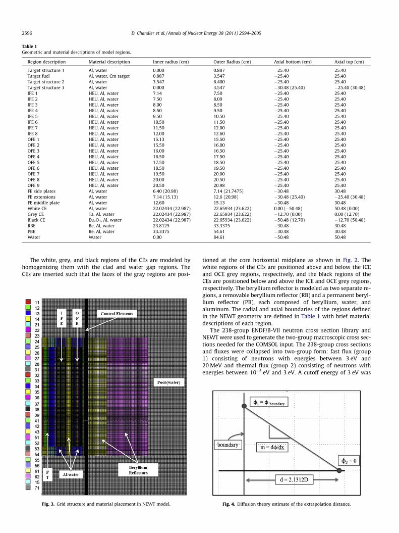
Table 1Geometric and material descriptions of model regions.

Region description Material description Inner radius (cm) Outer Radius (cm) Axial bottom (cm) Axial top (cm)

Target structure 1 Al, water 0.000 0.887 �25.40 25.40Target fuel Al, water, Cm target 0.887 3.547 �25.40 25.40Target structure 2 Al, water 3.547 6.400 �25.40 25.40Target structure 3 Al, water 0.000 3.547 �30.48 (25.40) �25.40 (30.48)IFE 1 HEU, Al, water 7.14 7.50 �25.40 25.40IFE 2 HEU, Al, water 7.50 8.00 �25.40 25.40IFE 3 HEU, Al, water 8.00 8.50 �25.40 25.40IFE 4 HEU, Al, water 8.50 9.50 �25.40 25.40IFE 5 HEU, Al, water 9.50 10.50 �25.40 25.40IFE 6 HEU, Al, water 10.50 11.50 �25.40 25.40IFE 7 HEU, Al, water 11.50 12.00 �25.40 25.40IFE 8 HEU, Al, water 12.00 12.60 �25.40 25.40OFE 1 HEU, Al, water 15.13 15.50 �25.40 25.40OFE 2 HEU, Al, water 15.50 16.00 �25.40 25.40OFE 3 HEU, Al, water 16.00 16.50 �25.40 25.40OFE 4 HEU, Al, water 16.50 17.50 �25.40 25.40OFE 5 HEU, Al, water 17.50 18.50 �25.40 25.40OFE 6 HEU, Al, water 18.50 19.50 �25.40 25.40OFE 7 HEU, Al, water 19.50 20.00 �25.40 25.40OFE 8 HEU, Al, water 20.00 20.50 �25.40 25.40OFE 9 HEU, Al, water 20.50 20.98 �25.40 25.40FE side plates Al, water 6.40 (20.98) 7.14 (21.7475) �30.48 30.48FE extensions Al, water 7.14 (15.13) 12.6 (20.98) �30.48 (25.40) �25.40 (30.48)FE middle plate Al, water 12.60 15.13 �30.48 30.48White CE Al, water 22.02434 (22.987) 22.65934 (23.622) 0.00 (�50.48) 50.48 (0.00)Grey CE Ta, Al, water 22.02434 (22.987) 22.65934 (23.622) �12.70 (0.00) 0.00 (12.70)Black CE Eu2O3, Al, water 22.02434 (22.987) 22.65934 (23.622) �50.48 (12.70) �12.70 (50.48)RBE Be, Al, water 23.8125 33.3375 �30.48 30.48PBE Be, Al, water 33.3375 54.61 �30.48 30.48Water Water 0.00 84.61 �50.48 50.48

2596 D. Chandler et al. / Annals of Nuclear Energy 38 (2011) 2594–2605

The white, grey, and black regions of the CEs are modeled byhomogenizing them with the clad and water gap regions. TheCEs are inserted such that the faces of the gray regions are posi-

Fig. 3. Grid structure and material placement in NEWT model.

tioned at the core horizontal midplane as shown in Fig. 2. Thewhite regions of the CEs are positioned above and below the ICEand OCE grey regions, respectively, and the black regions of theCEs are positioned below and above the ICE and OCE grey regions,respectively. The beryllium reflector is modeled as two separate re-gions, a removable beryllium reflector (RB) and a permanent beryl-lium reflector (PB), each composed of beryllium, water, andaluminum. The radial and axial boundaries of the regions definedin the NEWT geometry are defined in Table 1 with brief materialdescriptions of each region.

The 238-group ENDF/B-VII neutron cross section library andNEWT were used to generate the two-group macroscopic cross sec-tions needed for the COMSOL input. The 238-group cross sectionsand fluxes were collapsed into two-group form: fast flux (group1) consisting of neutrons with energies between 3 eV and20 MeV and thermal flux (group 2) consisting of neutrons withenergies between 10�5 eV and 3 eV. A cutoff energy of 3 eV was

Fig. 4. Diffusion theory estimate of the extrapolation distance.

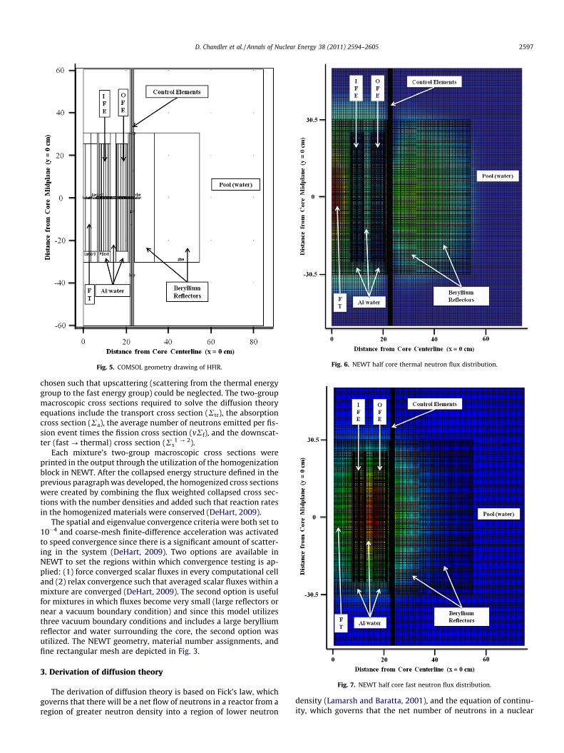
Fig. 5. COMSOL geometry drawing of HFIR. Fig. 6. NEWT half core thermal neutron flux distribution.

Fig. 7. NEWT half core fast neutron flux distribution.


chosen such that upscattering (scattering from the thermal energygroup to the fast energy group) could be neglected. The two-groupmacroscopic cross sections required to solve the diffusion theoryequations include the transport cross section (Rtr), the absorptioncross section (Ra), the average number of neutrons emitted per fis-sion event times the fission cross section (vRf), and the downscat-ter (fast ? thermal) cross section (Rs

1 ? 2).Each mixture’s two-group macroscopic cross sections were

printed in the output through the utilization of the homogenizationblock in NEWT. After the collapsed energy structure defined in theprevious paragraph was developed, the homogenized cross sectionswere created by combining the flux weighted collapsed cross sec-tions with the number densities and added such that reaction ratesin the homogenized materials were conserved (DeHart, 2009).

The spatial and eigenvalue convergence criteria were both set to10�4 and coarse-mesh finite-difference acceleration was activatedto speed convergence since there is a significant amount of scatter-ing in the system (DeHart, 2009). Two options are available inNEWT to set the regions within which convergence testing is ap-plied: (1) force converged scalar fluxes in every computational celland (2) relax convergence such that averaged scalar fluxes within amixture are converged (DeHart, 2009). The second option is usefulfor mixtures in which fluxes become very small (large reflectors ornear a vacuum boundary condition) and since this model utilizesthree vacuum boundary conditions and includes a large berylliumreflector and water surrounding the core, the second option wasutilized. The NEWT geometry, material number assignments, andfine rectangular mesh are depicted in Fig. 3.

3. Derivation of diffusion theory

The derivation of diffusion theory is based on Fick’s law, whichgoverns that there will be a net flow of neutrons in a reactor from aregion of greater neutron density into a region of lower neutron

density (Lamarsh and Baratta, 2001), and the equation of continu-ity, which governs that the net number of neutrons in a nuclear

Fig. 8. COMSOL half core thermal neutron flux distribution.


system must be conserved. The expression for Fick’s law is shownin Eq. (1) and the expression for neutron continuity is shown in Eq.(2). For a complete derivation of these relationships refer to Stacey(2001) and Lamarsh and Baratta (2001).

�J ¼ �Dr/ ð1Þ

where �J is the neutron current density vector, D is the diffusioncoefficient ¼ 1

3Rtr

� �, r is the gradient operator ¼ d

dxþ ddyþ d

dz

� �in

rectangular coordinates, / is the neutron flux.Zdndt

dV ¼Z

SdV �Z

Ra/dV �Zr ��JdV ð2Þ

The left-hand side (LHS) of Eq. (2) represents the time rate ofchange of the number of neutrons in volume V. The productionrate in V, absorption rate in V, and the net leakage from the sur-faces of V are shown from left to right on the right-hand side(RHS) of Eq. (2). The diffusion equation is developed by substitut-ing Fick’s law into the equation of neutron continuity and isshown in Eq. (3)

dndt¼ S� Ra/� Dr2/ ð3Þ

The focus of this study is to obtain the steady-state BOC fluxesand thus the time-dependence term can be neglected. Also, no exter-nal sources are present in HFIR and therefore fission is the only con-tributor to the production rate, S. Thus, the steady-state one-groupdiffusion equation with no external sources is written in the form of

vRf/� Ra/þ Dr2/ ¼ 0 ð4Þ

Since two energy groups are being studied in this analysis, scat-tering from one energy group to another must be included into thediffusion equation. The two-group neutron diffusion equations forfast (group 1: noted with subscript 1) and thermal (group 2: notedwith subscript 2) fluxes assuming all fission neutrons are born as fastneutrons are shown in Eqs. (5) and (6), respectively. The equationswere rearranged such that the LHS of the equations describe theneutron loss mechanism and the RHS of the equations describe theneutron production mechanism. The effective multiplication factor,keff, was also inserted to balance the equations and describes howthe population of neutrons varies from one generation to another.

�D1r2/1 þ ðRa1 þ R1!2s Þ/1 ¼

1keffðvRf1/1 þ vRf2/2Þ þ R2!1

s /2

ð5Þ

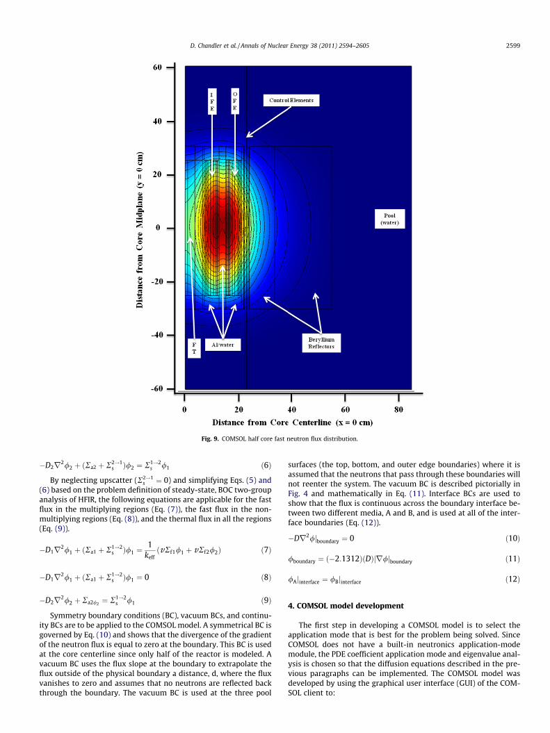
Fig. 9. COMSOL half core fast neutron flux distribution.


�D2r2/2 þ ðRa2 þ R2!1s Þ/2 ¼ R1!2

s /1 ð6Þ

By neglecting upscatter (R2!1s ¼ 0) and simplifying Eqs. (5) and

(6) based on the problem definition of steady-state, BOC two-groupanalysis of HFIR, the following equations are applicable for the fastflux in the multiplying regions (Eq. (7)), the fast flux in the non-multiplying regions (Eq. (8)), and the thermal flux in all the regions(Eq. (9)).

�D1r2/1 þ ðRa1 þ R1!2s Þ/1 ¼

1keffðvRf1/1 þ vRf2/2Þ ð7Þ

�D1r2/1 þ ðRa1 þ R1!2s Þ/1 ¼ 0 ð8Þ

�D2r2/2 þ Ra2/2 ¼ R1!2s /1 ð9Þ

Symmetry boundary conditions (BC), vacuum BCs, and continu-ity BCs are to be applied to the COMSOL model. A symmetrical BC isgoverned by Eq. (10) and shows that the divergence of the gradientof the neutron flux is equal to zero at the boundary. This BC is usedat the core centerline since only half of the reactor is modeled. Avacuum BC uses the flux slope at the boundary to extrapolate theflux outside of the physical boundary a distance, d, where the fluxvanishes to zero and assumes that no neutrons are reflected backthrough the boundary. The vacuum BC is used at the three pool

surfaces (the top, bottom, and outer edge boundaries) where it isassumed that the neutrons that pass through these boundaries willnot reenter the system. The vacuum BC is described pictorially inFig. 4 and mathematically in Eq. (11). Interface BCs are used toshow that the flux is continuous across the boundary interface be-tween two different media, A and B, and is used at all of the inter-face boundaries (Eq. (12)).

�Dr2/jboundary ¼ 0 ð10Þ

/boundary ¼ ð�2:1312ÞðDÞjr/jboundary ð11Þ

/Ajinterface ¼ /Bjinterface ð12Þ

4. COMSOL model development

The first step in developing a COMSOL model is to select theapplication mode that is best for the problem being solved. SinceCOMSOL does not have a built-in neutronics application-modemodule, the PDE coefficient application mode and eigenvalue anal-ysis is chosen so that the diffusion equations described in the pre-vious paragraphs can be implemented. The COMSOL model wasdeveloped by using the graphical user interface (GUI) of the COM-SOL client to:

Fig. 10. Thermal (middle) and fast (right) flux in the flux trap (h = 60.96 cm,r = 6.4 cm).


(a) create the identical geometry that was utilized in the NEWTmodel,

(b) import the macroscopic cross sections previously calculatedby NEWT,

(c) code the diffusion theory equations into the subdomainsettings,

(d) define the appropriate boundary conditions in the boundarysettings,

(e) create an appropriately fine mesh,(f) set up the solver, and finally,(g) perform the actual calculation.

The two-dimensional HFIR COMSOL model as it appears in thedraw mode of the GUI is shown in Fig. 5. The same dimensions de-fined in the NEWT model (Table 1) were utilized in the COMSOLmodel.

The PDE coefficient mode allows the user to enter a system ofPDEs into the software in the form expressed in Eq. (13). Theequations entered in the subdomain settings GUI for the fast fluxin the multiplying regions, the fast flux in the non-multiplying re-gions, and the thermal flux in all the regions are shown inEqs. (14)–(16), respectively. The subscripts 1 and 2 indicate fastand thermal energy groups, respectively.

r � ð�cru� auþ cÞ þ auþ b � ru

¼ daðk� k0Þu� eaðk� k0Þ2uþ f ð13Þ

where c is the diffusion coefficient, u is the dependent variable, a isthe conservative flux convection coefficient, c is the conservativeflux source term, a is the absorption coefficient, b is the convectioncoefficient, da is the damping/mass coefficient, k is the eigenvalue,k0 is the linearization point for the eigenvalue, ea is the mass coef-ficient, and f is the source term.

r � ð�D1r/1Þ þ ðRa1 þ R1!2s Þ/1

¼ k/1 þ1

keffðvRf1/1 þ vRf2/2Þ ð14Þ

r � ð�D1r/1Þ þ ðRa1 þ R1!2s Þ/1 ¼ k/1 ð15Þ

r � ð�D2r/2Þ þ Ra2/2 ¼ k/2 þ R1!2s /1 ð16Þ

Two PDE coefficient modes are coupled together and dependentupon each other since the thermal and fast neutron fluxes arebeing solved. The dependent variable for the first mode is the fastflux and the dependent variable for the second mode is the thermalflux. Thus, Eqs. (14) and (15) are input for the multiplying and non-multiplying regions, respectively, in the fast flux PDE coefficientmode and Eq. (16) is input for the multiplying and non-multiplyingregions in the thermal flux PDE coefficient mode. Since there are 31unique materials in the model there are 31 distinct equations spec-ified for the fast flux and 31 distinct equations for the thermal flux(62 distinct sets of cross sections and diffusion coefficients).

The boundary conditions were defined in the boundary settingsGUI. Boundary conditions were defined for both the fast and ther-mal flux physics modes. Symmetry was used at the core centerline,vacuum BCs were applied at the three outer pool boundaries, andcontinuity BCs were used at all of the inner surfaces. The governingequations for the boundary conditions are shown in Eqs. (17)–(22).The first equation listed for each BC is written in ‘‘generic’’ termsand the second equation listed for each BC is the equation appliedto the COMSOL model.

Symmetry – Neumann boundary condition:

n � ðcruþ au� cÞ þ qu ¼ g ð17Þ

n � ðDr/Þ ¼ 0 ð18Þ

Vacuum – Dirichlet boundary condition:

hu ¼ r ð19Þ

/ ¼ ð�2:1312ÞðDÞjr/jboundary ð20Þ

Continuity – Neumann boundary condition:

n � ððcruþ au� cÞ1 � ðcruþ au� cÞ2Þ þ qu ¼ g ð21Þ

n � ððDr/Þ1 � ðDr/Þ2Þ ¼ 0 ð22Þ

COMSOL provides an adaptive mesh refinement algorithm thatprovides an iterative solution scheme to update the mesh based onthe results from the solution. In this manner, machine accuracymay be obtained in the solution, thus yielding only round-off errorleft in the solution. The automatic mesh refinement algorithm wasused to solve the diffusion equations using a sequence of refinedmeshes. The predefined ‘‘extremely course’’ triangular mesh wasused as the initial mesh and was refined five times by the ‘‘longestedge’’ refinement method. When using the ‘‘longest edge’’ refine-ment method, the longest edge of the triangles that are determinedto have the largest errors are bisected in order to increase the num-ber of elements in areas of largest numerical error. The initial meshwas used to solve the system of PDEs and was improved by

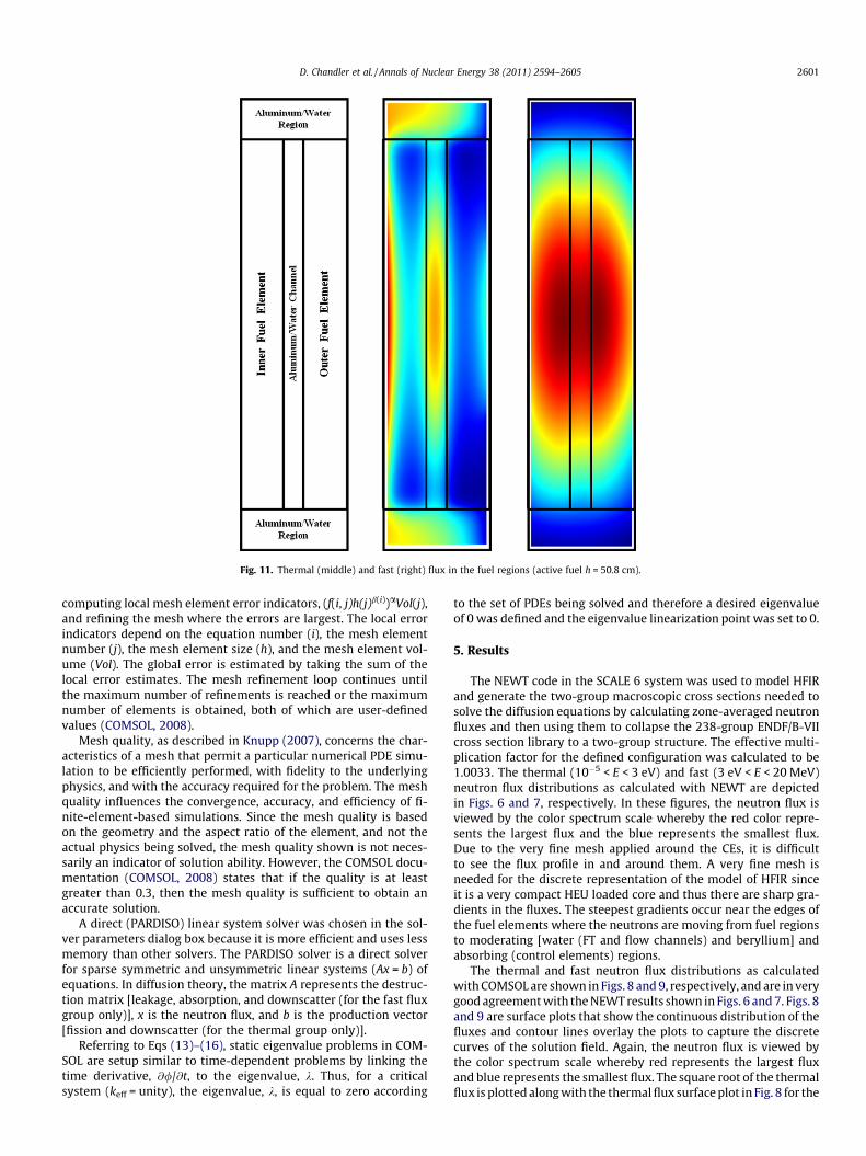
Fig. 11. Thermal (middle) and fast (right) flux in the fuel regions (active fuel h = 50.8 cm).


computing local mesh element error indicators, (f(i, j)h(j)b(i))aVol(j),and refining the mesh where the errors are largest. The local errorindicators depend on the equation number (i), the mesh elementnumber (j), the mesh element size (h), and the mesh element vol-ume (Vol). The global error is estimated by taking the sum of thelocal error estimates. The mesh refinement loop continues untilthe maximum number of refinements is reached or the maximumnumber of elements is obtained, both of which are user-definedvalues (COMSOL, 2008).

Mesh quality, as described in Knupp (2007), concerns the char-acteristics of a mesh that permit a particular numerical PDE simu-lation to be efficiently performed, with fidelity to the underlyingphysics, and with the accuracy required for the problem. The meshquality influences the convergence, accuracy, and efficiency of fi-nite-element-based simulations. Since the mesh quality is basedon the geometry and the aspect ratio of the element, and not theactual physics being solved, the mesh quality shown is not neces-sarily an indicator of solution ability. However, the COMSOL docu-mentation (COMSOL, 2008) states that if the quality is at leastgreater than 0.3, then the mesh quality is sufficient to obtain anaccurate solution.

A direct (PARDISO) linear system solver was chosen in the sol-ver parameters dialog box because it is more efficient and uses lessmemory than other solvers. The PARDISO solver is a direct solverfor sparse symmetric and unsymmetric linear systems (Ax = b) ofequations. In diffusion theory, the matrix A represents the destruc-tion matrix [leakage, absorption, and downscatter (for the fast fluxgroup only)], x is the neutron flux, and b is the production vector[fission and downscatter (for the thermal group only)].

Referring to Eqs (13)–(16), static eigenvalue problems in COM-SOL are setup similar to time-dependent problems by linking thetime derivative, @//@t, to the eigenvalue, k. Thus, for a criticalsystem (keff = unity), the eigenvalue, k, is equal to zero according

to the set of PDEs being solved and therefore a desired eigenvalueof 0 was defined and the eigenvalue linearization point was set to 0.

5. Results

The NEWT code in the SCALE 6 system was used to model HFIRand generate the two-group macroscopic cross sections needed tosolve the diffusion equations by calculating zone-averaged neutronfluxes and then using them to collapse the 238-group ENDF/B-VIIcross section library to a two-group structure. The effective multi-plication factor for the defined configuration was calculated to be1.0033. The thermal (10�5 < E < 3 eV) and fast (3 eV < E < 20 MeV)neutron flux distributions as calculated with NEWT are depictedin Figs. 6 and 7, respectively. In these figures, the neutron flux isviewed by the color spectrum scale whereby the red color repre-sents the largest flux and the blue represents the smallest flux.Due to the very fine mesh applied around the CEs, it is difficultto see the flux profile in and around them. A very fine mesh isneeded for the discrete representation of the model of HFIR sinceit is a very compact HEU loaded core and thus there are sharp gra-dients in the fluxes. The steepest gradients occur near the edges ofthe fuel elements where the neutrons are moving from fuel regionsto moderating [water (FT and flow channels) and beryllium] andabsorbing (control elements) regions.

The thermal and fast neutron flux distributions as calculatedwith COMSOL are shown in Figs. 8 and 9, respectively, and are in verygood agreement with the NEWT results shown in Figs. 6 and 7. Figs. 8and 9 are surface plots that show the continuous distribution of thefluxes and contour lines overlay the plots to capture the discretecurves of the solution field. Again, the neutron flux is viewed bythe color spectrum scale whereby red represents the largest fluxand blue represents the smallest flux. The square root of the thermalflux is plotted along with the thermal flux surface plot in Fig. 8 for the

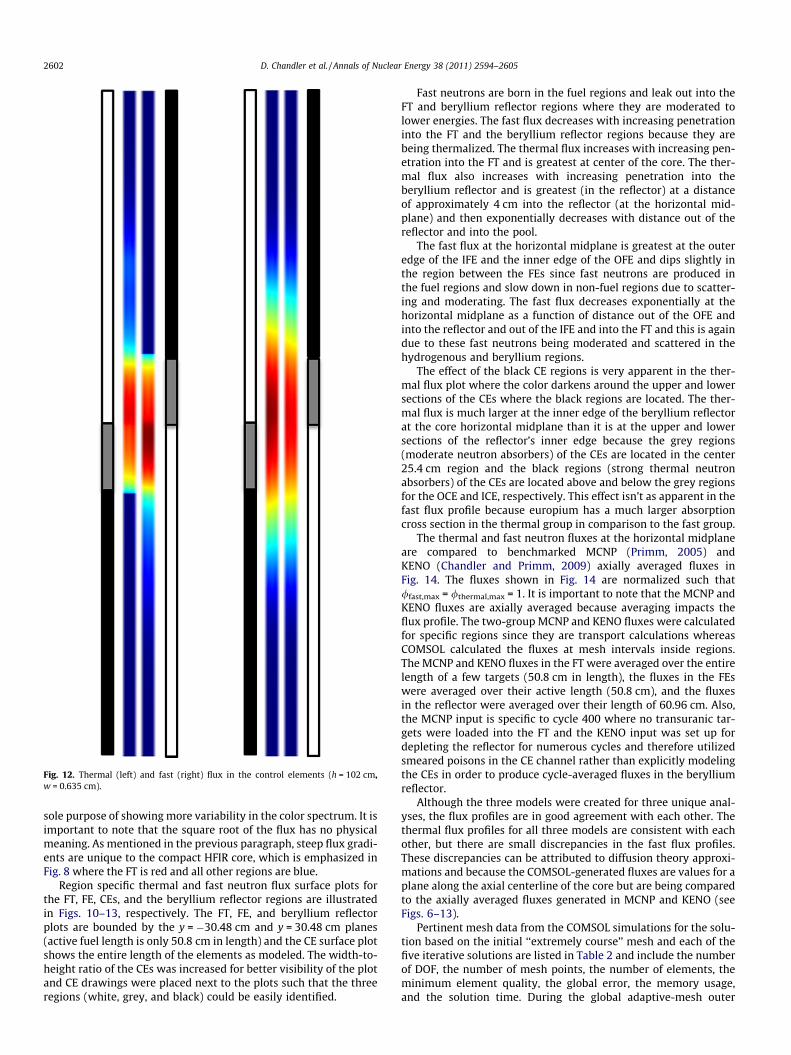
Fig. 12. Thermal (left) and fast (right) flux in the control elements (h = 102 cm,w = 0.635 cm).


sole purpose of showing more variability in the color spectrum. It isimportant to note that the square root of the flux has no physicalmeaning. As mentioned in the previous paragraph, steep flux gradi-ents are unique to the compact HFIR core, which is emphasized inFig. 8 where the FT is red and all other regions are blue.

Region specific thermal and fast neutron flux surface plots forthe FT, FE, CEs, and the beryllium reflector regions are illustratedin Figs. 10–13, respectively. The FT, FE, and beryllium reflectorplots are bounded by the y = �30.48 cm and y = 30.48 cm planes(active fuel length is only 50.8 cm in length) and the CE surface plotshows the entire length of the elements as modeled. The width-to-height ratio of the CEs was increased for better visibility of the plotand CE drawings were placed next to the plots such that the threeregions (white, grey, and black) could be easily identified.

Fast neutrons are born in the fuel regions and leak out into theFT and beryllium reflector regions where they are moderated tolower energies. The fast flux decreases with increasing penetrationinto the FT and the beryllium reflector regions because they arebeing thermalized. The thermal flux increases with increasing pen-etration into the FT and is greatest at center of the core. The ther-mal flux also increases with increasing penetration into theberyllium reflector and is greatest (in the reflector) at a distanceof approximately 4 cm into the reflector (at the horizontal mid-plane) and then exponentially decreases with distance out of thereflector and into the pool.

The fast flux at the horizontal midplane is greatest at the outeredge of the IFE and the inner edge of the OFE and dips slightly inthe region between the FEs since fast neutrons are produced inthe fuel regions and slow down in non-fuel regions due to scatter-ing and moderating. The fast flux decreases exponentially at thehorizontal midplane as a function of distance out of the OFE andinto the reflector and out of the IFE and into the FT and this is againdue to these fast neutrons being moderated and scattered in thehydrogenous and beryllium regions.

The effect of the black CE regions is very apparent in the ther-mal flux plot where the color darkens around the upper and lowersections of the CEs where the black regions are located. The ther-mal flux is much larger at the inner edge of the beryllium reflectorat the core horizontal midplane than it is at the upper and lowersections of the reflector’s inner edge because the grey regions(moderate neutron absorbers) of the CEs are located in the center25.4 cm region and the black regions (strong thermal neutronabsorbers) of the CEs are located above and below the grey regionsfor the OCE and ICE, respectively. This effect isn’t as apparent in thefast flux profile because europium has a much larger absorptioncross section in the thermal group in comparison to the fast group.

The thermal and fast neutron fluxes at the horizontal midplaneare compared to benchmarked MCNP (Primm, 2005) andKENO (Chandler and Primm, 2009) axially averaged fluxes inFig. 14. The fluxes shown in Fig. 14 are normalized such that/fast,max = /thermal,max = 1. It is important to note that the MCNP andKENO fluxes are axially averaged because averaging impacts theflux profile. The two-group MCNP and KENO fluxes were calculatedfor specific regions since they are transport calculations whereasCOMSOL calculated the fluxes at mesh intervals inside regions.The MCNP and KENO fluxes in the FT were averaged over the entirelength of a few targets (50.8 cm in length), the fluxes in the FEswere averaged over their active length (50.8 cm), and the fluxesin the reflector were averaged over their length of 60.96 cm. Also,the MCNP input is specific to cycle 400 where no transuranic tar-gets were loaded into the FT and the KENO input was set up fordepleting the reflector for numerous cycles and therefore utilizedsmeared poisons in the CE channel rather than explicitly modelingthe CEs in order to produce cycle-averaged fluxes in the berylliumreflector.

Although the three models were created for three unique anal-yses, the flux profiles are in good agreement with each other. Thethermal flux profiles for all three models are consistent with eachother, but there are small discrepancies in the fast flux profiles.These discrepancies can be attributed to diffusion theory approxi-mations and because the COMSOL-generated fluxes are values for aplane along the axial centerline of the core but are being comparedto the axially averaged fluxes generated in MCNP and KENO (seeFigs. 6–13).

Pertinent mesh data from the COMSOL simulations for the solu-tion based on the initial ‘‘extremely course’’ mesh and each of thefive iterative solutions are listed in Table 2 and include the numberof DOF, the number of mesh points, the number of elements, theminimum element quality, the global error, the memory usage,and the solution time. During the global adaptive-mesh outer

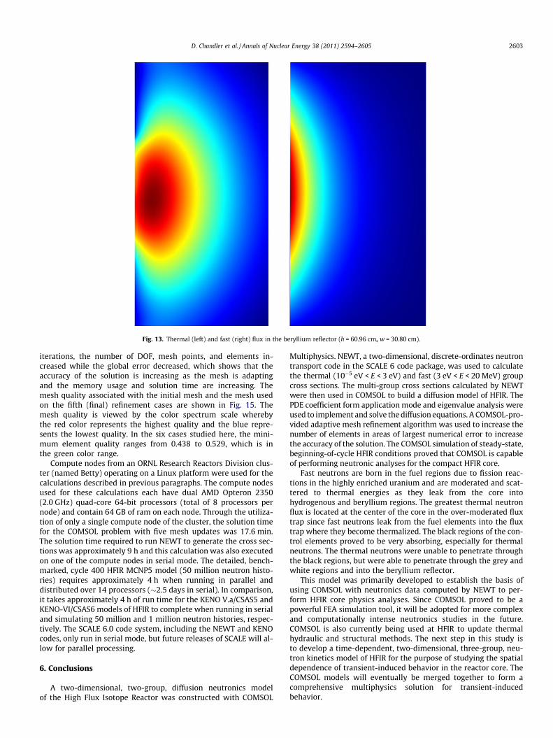
Fig. 13. Thermal (left) and fast (right) flux in the beryllium reflector (h = 60.96 cm, w = 30.80 cm).


iterations, the number of DOF, mesh points, and elements in-creased while the global error decreased, which shows that theaccuracy of the solution is increasing as the mesh is adaptingand the memory usage and solution time are increasing. Themesh quality associated with the initial mesh and the mesh usedon the fifth (final) refinement cases are shown in Fig. 15. Themesh quality is viewed by the color spectrum scale wherebythe red color represents the highest quality and the blue repre-sents the lowest quality. In the six cases studied here, the mini-mum element quality ranges from 0.438 to 0.529, which is inthe green color range.

Compute nodes from an ORNL Research Reactors Division clus-ter (named Betty) operating on a Linux platform were used for thecalculations described in previous paragraphs. The compute nodesused for these calculations each have dual AMD Opteron 2350(2.0 GHz) quad-core 64-bit processors (total of 8 processors pernode) and contain 64 GB of ram on each node. Through the utiliza-tion of only a single compute node of the cluster, the solution timefor the COMSOL problem with five mesh updates was 17.6 min.The solution time required to run NEWT to generate the cross sec-tions was approximately 9 h and this calculation was also executedon one of the compute nodes in serial mode. The detailed, bench-marked, cycle 400 HFIR MCNP5 model (50 million neutron histo-ries) requires approximately 4 h when running in parallel anddistributed over 14 processors (�2.5 days in serial). In comparison,it takes approximately 4 h of run time for the KENO V.a/CSAS5 andKENO-VI/CSAS6 models of HFIR to complete when running in serialand simulating 50 million and 1 million neutron histories, respec-tively. The SCALE 6.0 code system, including the NEWT and KENOcodes, only run in serial mode, but future releases of SCALE will al-low for parallel processing.

6. Conclusions

A two-dimensional, two-group, diffusion neutronics modelof the High Flux Isotope Reactor was constructed with COMSOL

Multiphysics. NEWT, a two-dimensional, discrete-ordinates neutrontransport code in the SCALE 6 code package, was used to calculatethe thermal (10�5 eV < E < 3 eV) and fast (3 eV < E < 20 MeV) groupcross sections. The multi-group cross sections calculated by NEWTwere then used in COMSOL to build a diffusion model of HFIR. ThePDE coefficient form application mode and eigenvalue analysis wereused to implement and solve the diffusion equations. A COMSOL-pro-vided adaptive mesh refinement algorithm was used to increase thenumber of elements in areas of largest numerical error to increasethe accuracy of the solution. The COMSOL simulation of steady-state,beginning-of-cycle HFIR conditions proved that COMSOL is capableof performing neutronic analyses for the compact HFIR core.

Fast neutrons are born in the fuel regions due to fission reac-tions in the highly enriched uranium and are moderated and scat-tered to thermal energies as they leak from the core intohydrogenous and beryllium regions. The greatest thermal neutronflux is located at the center of the core in the over-moderated fluxtrap since fast neutrons leak from the fuel elements into the fluxtrap where they become thermalized. The black regions of the con-trol elements proved to be very absorbing, especially for thermalneutrons. The thermal neutrons were unable to penetrate throughthe black regions, but were able to penetrate through the grey andwhite regions and into the beryllium reflector.

This model was primarily developed to establish the basis ofusing COMSOL with neutronics data computed by NEWT to per-form HFIR core physics analyses. Since COMSOL proved to be apowerful FEA simulation tool, it will be adopted for more complexand computationally intense neutronics studies in the future.COMSOL is also currently being used at HFIR to update thermalhydraulic and structural methods. The next step in this study isto develop a time-dependent, two-dimensional, three-group, neu-tron kinetics model of HFIR for the purpose of studying the spatialdependence of transient-induced behavior in the reactor core. TheCOMSOL models will eventually be merged together to form acomprehensive multiphysics solution for transient-inducedbehavior.

0.0

0.1

0.2

0.3

0.4

0.5

0.6

0.7

0.8

0.9

1.0

1.1

0 5 10 15 20 25 30 35 40 45 50 55 60

Nor

mal

ized

Flu

x

Distance from Core Centerline

COMSOL (thermal at horizontal midplane)

MCNP (thermal axially averaged)

KENO VI (thermal axially averaged)

COMSOL (fast at horizontal midplane)

MCNP (fast axially averaged)

KENO VI (fast axially averaged)

Beryllium Reflector

OFEIFEFT

Note: flux trap in MCNP model has no transuranic targets and MCNP/KENO fluxes are axially averaged whereas COMSOL fluxes are at the core horizontal midplane.

Wat

er R

efle

ctor

Fig. 14. Normalized two-group flux profiles.

Fig. 15. COMSOL mesh quality (mesh refinement 0 on left, mesh refinement 5 on right).


Table 2Automatic mesh refinement statistics/parameters.

Mesh refinement DOF Mesh points Elements Min. element quality Global error Memory (GB) Cumulative solution time (s) Solution time (s)

0 5.016E+04 6.293E+03 1.250E+04 0.529 3.024E�01 4.7 5.2 5.21 1.615E+05 2.024E+04 4.025E+04 0.438 5.147E�03 5.0 31.4 26.22 3.510E+05 4.398E+04 8.757E+04 0.438 1.591E�03 5.4 82.6 51.13 7.010E+05 8.778E+04 1.749E+05 0.438 6.924E-04 6.4 185.6 103.04 1.335E+06 1.671E+05 3.331E+05 0.464 3.229E�04 8.2 392.0 206.55 2.501E+06 3.129E+05 6.244E+05 0.438 1.646E�04 11.0 1054.0 662.0


Acknowledgements

This manuscript has been authored by UT-Battelle, LLC, underContract No. DE-AC05-00OR22725 with the US Department of En-ergy. The United States Government retains and the publisher, byaccepting the article for publication, acknowledges that the UnitedStates Government retains a non-exclusive, paid-up, irrevocable,world-wide license to publish or reproduce the published form ofthis manuscript, or allow others to do so, for United States Govern-ment purposes.

References

Chandler, D., Primm III, R.T., Maldonado, G.I., 2009. Reactivity AccountabilityAttributed to Beryllium Reflector Poisons in the High Flux Isotope Reactor,ORNL/TM-2009/188, December 2009.

COMSOL, 2008. COMSOL, Inc., COMSOL Multiphysics User’s Guide, Version 3.5a,Burlington, MA.

DeHart, M.D., 2009. NEWT: A New Transport Algorithm for Two-DimensionalDiscrete Ordinates Analysis in Non-Orthogonal Geometries, ORNL/TM-2005/39,Version 6, vol. II.

Gomes, G., 2008. Comparison between COMSOL and RFSP-IST for a 2-D BenchmarkProblem, Atomic Energy of Canada Limited, Excerpt from the Proceedings of theCOMSOL Conference 2008 Hannover, Germany, November 2008.

Knupp, P.M., 2007. Remarks on Mesh Quality, Sandia National Laboratory, Paperfrom the 45th American Institute of Aeronautics and Astronautics AerospaceSciences Meeting and Exhibit 2007, Reno, NV.

Lamarsh, J.R., Baratta, A.J., 2001. Introduction to Nuclear Engineering, third ed.Prentice Hall, New Jersey.

Memoli, V., et al. 2009. A Preliminary Approach to the Neutronics of the Molten SaltReactor by means of COMSOL Multiphysics, Politecnico di Milano, Excerpt fromthe Proceedings of the COMSOL Conference 2009 Milan.

Primm III, R.T., Xoubi, N., 2005. Modeling of the High Flux Isotope Reactor Cycle 400,ORNL/TM-2004/251, Oak Ridge National Laboratory, August 2005.

Primm III, R.T., et al., 2009. Design Study for a Low Enriched Uranium Core for theHigh Flux Isotope Reactor, ORNL/TM-2009/87, Oak Ridge National Laboratory,March 2009.

Primm III, R.T., et al., 2011. Design Study for a Low-Enriched Uranium Core for theHigh Flux Isotope Reactor, Annual Report for FY 2010, ORNL/TM-2011/06, OakRidge National Laboratory.

SCALE: A Modular Code system for Performing Standardized Computer Analyses forLicensing Evaluations, ORNL/TM-2005/39, Version 6, vols. I–III, January 2009.Available from Radiation Safety Information Computational Center at Oak RidgeNational Laboratory.

Stacey, W.M., 2001. Nuclear Reactor Physics. John Wiley and Sons, Inc., New York.

neutronics modeling of the high flux isotope reactor using comsol

Documents