neural networks pattern association chapter 3. neural networks3: pattern association2 pattern...

Neural Networks

Pattern Association

CHAPTER 3

Neural Networks3: Pattern Association 2

Pattern Association learning is the process of forming associations

between related patterns. The patterns we associate together may be of the

same type or of different types. Memorization of a pattern may be considered to be

associating the pattern with itself. An important characteristic of the associations we

form is that an input stimulus which is similar to the stimulus for the association will invoke the associated response pattern (recognizing a person in a photo or playing new music notes).


Pattern Association Each association is an input-output vector pair, s:t. If each vector t is the same as the vector s with

which it is associated, then the net is called an autoassociative memory.

If the t's are different from the s's, the net is called a heteroassociative memory.

In each of these cases, the net not only learns the specific pattern pairs that were used for training, but also is able to recall the desired response pattern when given an input stimulus that is similar, but not identical, to the training input.


Training Hebb Rule for Pattern Association The Hebb rule is the simplest and most common

method of determining the weights for an associative memory neural net.

It can be used with patterns that are represented as either binary or bipolar vectors


Algorithm


Outer products The weights found by using the Hebb rule (with all

weights initially 0) can also be described in terms of outer products of the input vector-output vector pairs.

The outer product of two vectors:


Outer products


Perfect recall versus cross talk

The suitability of the Hebb rule for a particular problem depends on the correlation among the input training vectors.

If the input vectors are uncorrelated (orthogonal), the Hebb rule will produce the correct weights, and the response of the net when tested with one of the training vectors will be perfect recall of the input vector's associated target .

If the input vectors are not orthogonal, the response will include a portion of each of their target values. This is commonly called cross talk.


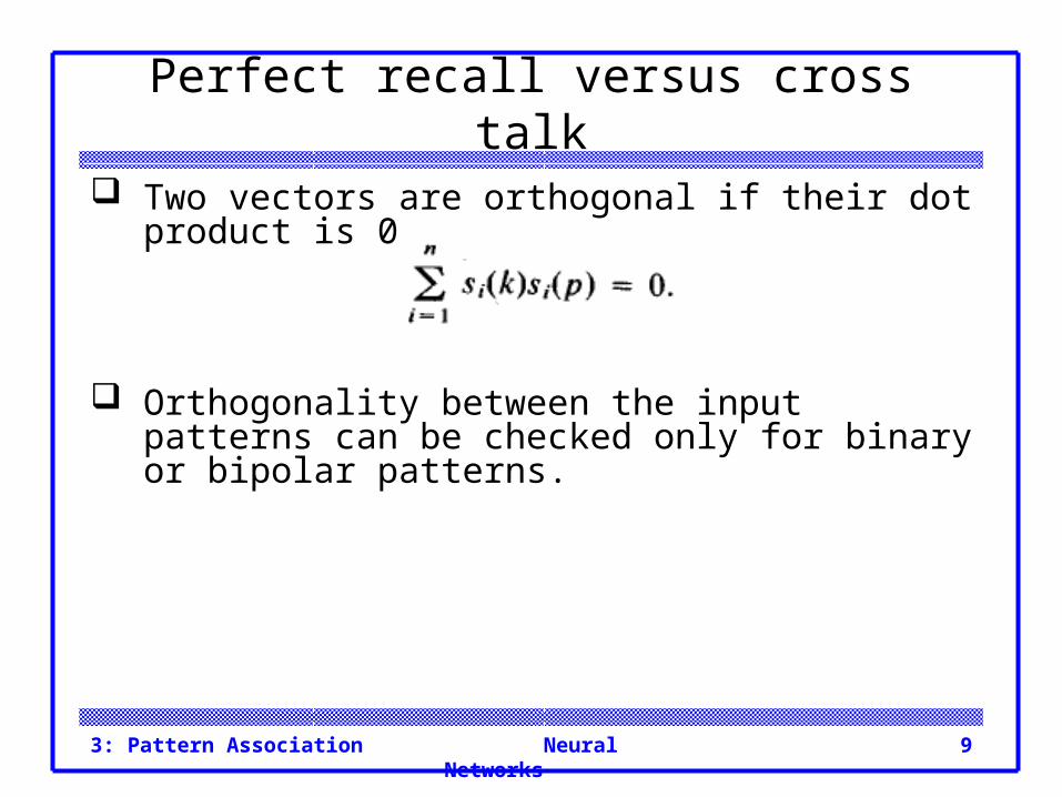
Perfect recall versus cross talk

Two vectors are orthogonal if their dot product is 0.

Orthogonality between the input patterns can be checked only for binary or bipolar patterns.


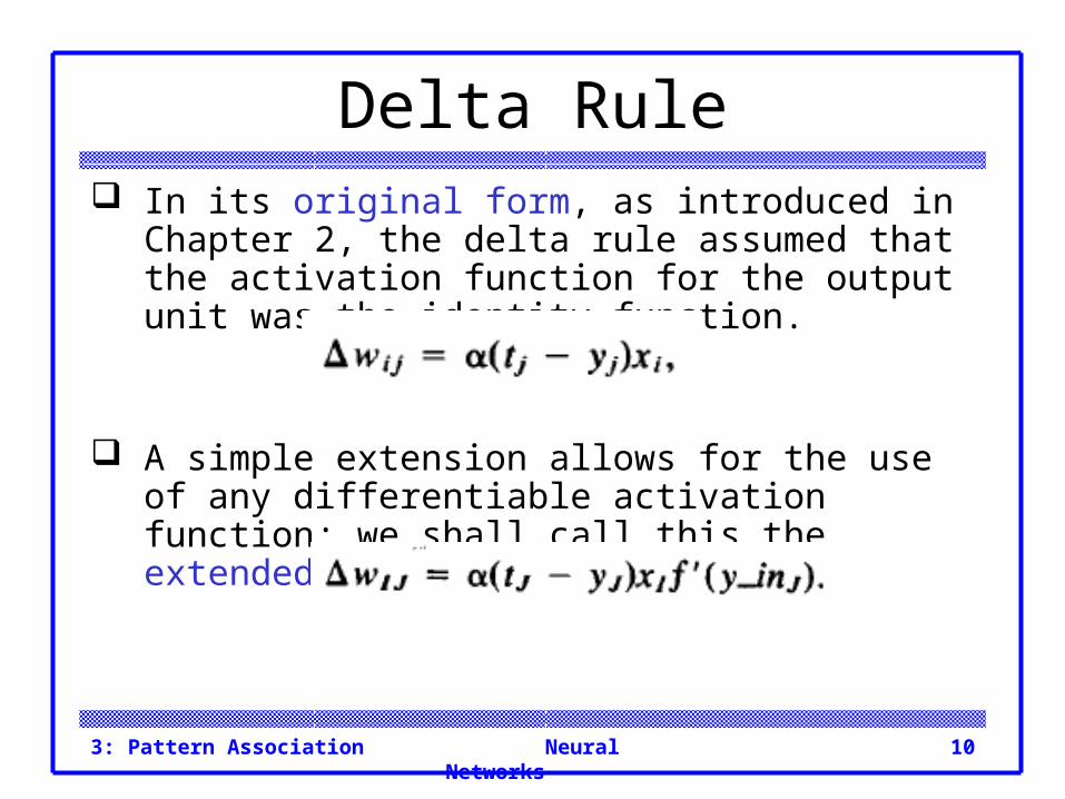
Delta Rule In its original form, as introduced in Chapter 2, the

delta rule assumed that the activation function for the output unit was the identity function.

A simple extension allows for the use of any differentiable activation function; we shall call this the extended delta rule.


Heteroassociative Memory

Associative memory neural networks are nets in which the weights are determined in such a way that the net can store a set of P pattern associations.

Each association is a pair of vectors (s(p), t(p)), with p = 1, 2, . . . , P.

Each vector s(p) is an n-tuple (has n components), and each t(p) is an m-tuple.

The weights may be found using the Hebb rule or the delta rule.


Architecture


Applications


Applications The output vector y gives the pattern associated with

the input vector x. This heteroassociative memory is not iterative.

If the target responses of the net are binary, a suitable activation function is given by


Applications A general form of the preceding activation function

that includes a threshold, and that is used in the bidirectional associative memory (BAM), an iterative net discussed in Section 3.5, is


Example 3.1 A Heteroassociative net trained using the Hebb rule. Suppose a net is to be trained to store the following

mapping from input row vectors s = ( s1, s2, s3, s4) to output row vectors t = (t1, t2).


Example 3.1


Example 3.1 These target patterns are simple enough that the

problem could be considered one in pattern classification; however, the process we describe here does not require that only one of the two output units be "on."

Also, the input vectors are not mutually orthogonal. However, because the target values are chosen to

be related to the input vectors in a particularly simple manner, the cross talk between the first and second input vectors does not pose any difficulties (since their target values are the same).


Example 3.1 The training is accomplished by the Hebb rule, which

is defined as:


Example 3.1 Training:


Example 3.1


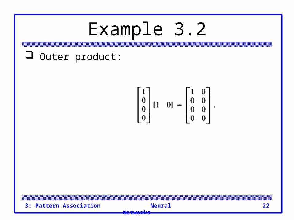
Example 3.2 Outer product:


Example 3.2 Second sample:


Example 3.2 Third sample:


Example 3.2 Fourth sample:


Example 3.2 Final W:


Example 3.3 Testing a heteroassociative net using the training

input. Activation function:

The weights are as found in Examples 3.1 and 3.2.


Example 3.3 First input: (the same for other inputs)


Example 3.3 Using Matrix (First input):


Example 3.4 Testing a heteroassociative net with input similar to

the training input. The test vector x = (0, 1, 0, 0) differs from the

training vector s = (1, 1, 0,0) only in the first component. We have:

Thus, the net also associates a known output pattern with this input.


Example 3.5 Testing a heteroassociative net with input that is not

similar to the traininginput.

The test pattern (0 1, 1, 0) differs from each of the training input patterns in at leas two components.


Example 3.5 The output is not one of the outputs with which the

net was trained; in other words, the net does not recognize the pattern.

In this case, we can view x = (0, 1, 1, 0) as differing from the training vector s = (1, 1, 0, 0) in the first and third components, so that the two "mistakes" in the input pattern make it impossible for the net to recognize it.

This is not surprising, since the vector could equally well be viewed as formed from s = (0, 0, 1, 1), with "mistakes" in the second and fourth components


Example 3.5 In general, a bipolar representation of our patterns is

computationally preferable to a binary representation.

In the first modification (Example 3.6), binary input and target vectors are converted to bipolar representations for the formation of the weight matrix. However, the input vectors used during testing and the response of the net are still represented in binary form.

In the second modification (Example 3.7), all vectors (training input, target output, testing input, and the response of the net) are expressed in bipolar form.


Example 3.6 A heteroassociative net using hybrid (binary/bipolar)

data representation to store a set of binary vector pairs s(p):t(p), p = 1,…

P, where:

using a weight matrix formed from the corresponding bipolar vectors, the weight matrix W = {wij} is given by:


Example 3.6 Using the data from Example 3.1, we have

The weight matrix that is obtained


Example 3.7 A heteroassociative net using bipolar vectors. To store a set of bipolar vector pairs s(p):t(p), p = 1, .

. . , P, where

the weight matrix W = {wij} is given by


Example 3.7 Using the data from Examples 3.1 through 3.6, we

have

The same weight matrix is obtained as in Example 3.6, namely,


Example 3.7 We illustrate the process of finding the weights using

outer products for this example. first pattern pair:


Example 3.7 second pattern pair:

Third pattern pair:


Example 3.7 Fourth pattern pair:

The weight matrix to store all four pattern pairs is the sum of the weight matrices:


Example 3.8 The effect of data representation: bipolar is better

than binary. Example 3.5 illustrated the difficulties that a simple

net (with binary input) experiences when given an input vector-with "mistakes" in two components.

The weight matrix formed from the bipolar representation of training patterns still cannot produce the proper response for an input vector formed from a stored vector with two "mistakes," e.g.,


Example 3.8 However, the net can respond correctly when given

an input vector formed from a stored vector with two components "missing.“

For example, consider the vector x = (0, 1, 0, - I), which is formed from the training vector s = (1, 1, - 1, -1I), with the first and third components "missing" rather than "wrong." We have:

the correct response for the stored vector s = (1, 1, - 1, - 1).


Example 3.9 A heteroassociative net for associating letters from

different fonts: A heteroassociative neural net was trained using the

Hebb rule (outer products) to associate three vector pairs.

The x vectors have 63 components, the y vectors 15.


Example 3.9 Training samples:


Example 3.9 The noise took the form of turning pixels "on" that

should have been "off" and vice versa. These are denoted as follows:


Example 3.9 Noisy samples and net response:


Example 3.9 Noisy samples with 30% noise :


AUTOASSOCIATIVE NET For an autoassociative net, the training input and

target output vectors are identical. The process of training is often called storing the

vectors, which may be binary or bipolar. The performance of the net is judged by its ability to

reproduce a stored pattern from noisy input; performance is, in general, better for bipolar vectors than for binary vectors.


AUTOASSOCIATIVE NET It is often the case that, for autoassociative nets, the

weights on the diagonal) are set to zero. Setting these weights to zero may improve the net's

ability to generalize or may increase the biological plausibility of the net.

Setting them to zero is necessary for extension to the iterative case or if the delta rule is used.


Architecture


Algorithm


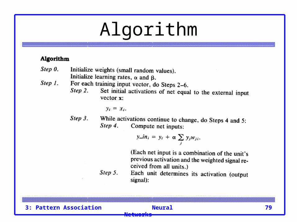
Algorithm As discussed earlier, in practice the weights are

usually set from the formula

rather than from the algorithmic form of Hebb learning.


Example 3.10 An autoassociative net to store one vector:

recognizing the stored vector. Step 0. The vector s = (1, 1, 1, - 1) is stored with the

weight matrix:

Step 1. For the testing input vector:– Step 2. x = (1, 1, 1, - 1).

– Step 3. y-in = (4, 4, 4, - 4).

– Step4. y = f ( 4 , 4 , 4 , - 4 ) = ( 1 , 1 , 1 , - 1 ) .


Example 3.10 The preceding process of using the net can be

written more succinctly as:

As before, the differences take one of two forms: "mistakes" in the data or "missing" data.

The only "mistakes" we consider are changes from + 1 to - 1 or vice versa.

We use the term "missing" data to refer to a component that has the value 0, rather than either + 1 or -1


Example 3.11 Testing an autoassociative net: one mistake in the

input vector.


Example 3.11 The reader can verify that the net also recognizes

the vectors formed when one component is "missing."

Those vectors are (0, 1, 1, -1), (1, 0, 1, - 1), (1, 1, 0, - 1), and (1, 1, 1, 0).

In general, a net is more tolerant of "missing" data than it is of "mistakes“ in the data, as the examples that follow demonstrate.


Example 3.12 Testing an autoassociative net: two "missing" entries

in the input vector. The vectors formed from (1, 1, 1, - 1) with two

"missing" data are (0, 0, 1, - 1),(0, 1, 0, -1), (0, 1, 1, 0), (1, 0, 0, -1), (1, 0, 1, 0), and (1, 1, 0, 0).


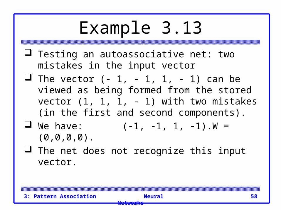
Example 3.13 Testing an autoassociative net: two mistakes in the

input vector The vector (- 1, - 1, 1, - 1) can be viewed as being

formed from the stored vector (1, 1, 1, - 1) with two mistakes (in the first and second components).

We have: (-1, -1, 1, -1).W = (0,0,0,0). The net does not recognize this input vector.


Example 3.14 An autoassociative net with no self-connections:

zeroing-out the diagonal. It is fairly common for an autoassociative network to

have its diagonal terms set to zero, e.g.,


Example 3.14 Consider again the input vector (- 1, - 1, 1, - 1)

formed from the stored vector (1, 1, 1, - 1) with two mistakes (in the first and second components).

We have:

The net still does not recognize this input vector.


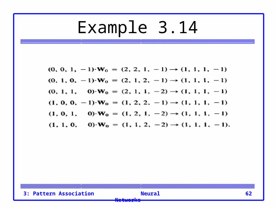
Example 3.14 It is interesting to note that if the weight matrix Wo is

used in the case of "missing" components in the input data, the output unit or units with the net input of largest magnitude coincide with the input unit or units whose input component or components were zero. We have:


Example 3.14


Storage Capacity An important consideration for associative memory

neural networks is the number of patterns or pattern pairs that can be stored before the net begins to forget.

The number of vectors that can be stored in a net is called the capacity of the net.


Example 3.15 Storing two vectors in an autoassociative net. More than one vector can be stored in an

autoassociative net by adding the weight matrices for each vector together.

For example, if W1 is the weight matrix used to store the vector (1, 1, - 1, - 1) and W2 is the weight matrix used to store the vector ( - 1, 1, 1, - 1), then the weight matrix used to store both (1, 1, - 1, - 1) and (- 1, 1, 1, - 1) is the sum of W1 and W2.


Example 3.15

The reader should verify that the net with weight matrix WI + W2 can recognize both of the vectors (1, 1, - 1, - 1) and ( - 1, 1, 1, - 1).


Example 3.16 Attempting to store two non-orthogonal vectors in an

autoassociative net. Not every pair of bipolar vectors can be stored in an

autoassociative net with four nodes; attempting to store the vectors (1, - 1, - 1, 1) and (1, 1, - 1, 1) by adding their weight matrices gives a net that cannot distinguish between the two vectors it was trained to recognize:


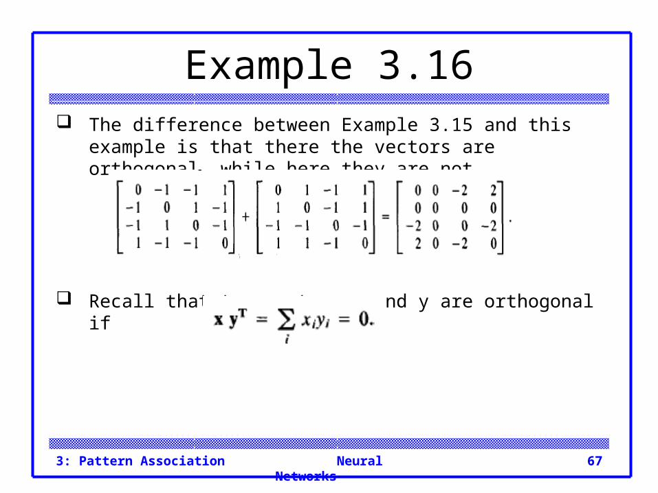
Example 3.16 The difference between Example 3.15 and this example is that

there the vectors are orthogonal, while here they are not.

Recall that two vectors x and y are orthogonal if


Example 3.16 An autoassociative net with four nodes can store three

orthogonal vectors (i.e., each vector is orthogonal to each of the other two vectors).


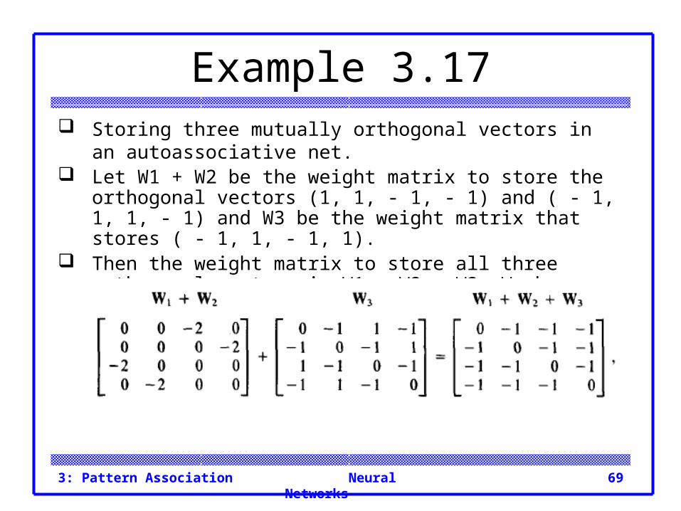
Example 3.17 Storing three mutually orthogonal vectors in an autoassociative

net. Let W1 + W2 be the weight matrix to store the orthogonal

vectors (1, 1, - 1, - 1) and ( - 1, 1, 1, - 1) and W3 be the weight matrix that stores ( - 1, 1, - 1, 1).

Then the weight matrix to store all three orthogonal vectors is W1 + W2 + W3. We have


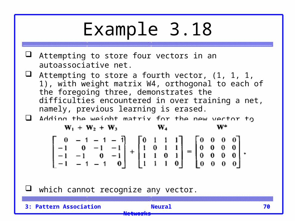
Example 3.18 Attempting to store four vectors in an autoassociative net. Attempting to store a fourth vector, (1, 1, 1, 1), with weight

matrix W4, orthogonal to each of the foregoing three, demonstrates the difficulties encountered in over training a net, namely, previous learning is erased.

Adding the weight matrix for the new vector to the matrix for the first three vectors gives:

which cannot recognize any vector.


Theorem The capacity of an autoassociative net depends on

the number of components the stored vectors have and the relationships among the stored vectors; more vectors can be stored if they are mutually orthogonal.

Expanding on ideas suggested by Szu (1989), we prove that n - 1 mutually orthogonal bipolar vectors, each with n components, can always be stored using the sum of the outer product weight matrices (with diagonal terms set to zero), but that attempting to store n mutually orthogonal vectors will result in a weight matrix that cannot reproduce any of the stored vectors.


ITERATIVE AUTOASSOCIATIVE NET

We see from the next example that in some cases the net does not respond immediately to an input signal with a stored target pattern, but the response may be enough like a stored pattern.


Example 3.19 Testing a recurrent autoassociative net: stored

vector with second, third and fourth components set to zero.

The weight matrix to store the vector (1, 1, 1, - 1) is

The vector (1,0,0,0) is an example of a vector formed from the stored vector with three "missing" components (three zero entries).


Example 3.19 The performance of the net for this vector is given

next. Input vector (1, 0, 0, 0):

– (1, 0, 0, 0).W = (0, 1, 1, - 1) iterate– (0, 1, 1, -1).W = (3,2,2, -2) (1, 1, 1, - 1).

Thus, for the input vector (1, 0, 0, O), the net produces the "known" vector ( 1 , 1, 1, - 1) as its response in two iterations.

For iterative nets, one key question is whether the activations will converge.


Recurrent Linear Autoassociator

One of the simplest iterative Autoassociator neural networks is known as the linear Autoassociator.

This net has n neurons, each connected to all of the other neurons.

The weight matrix is symmetric, with the connection strength wij proportional to the sum over all training patterns of the product of the activations of the two units xi and xj.

In other words, the weights can be found by the Hebb rule.

McClelland and Rumelhart do not restrict the weight matrix to have zeros on the diagonal.



An n x n nonsingular symmetric matrix (such as the weight matrix) has n mutually orthogonal eigenvectors.

A recurrent linear Autoassociator neural net is trained using a set of K orthogonal unit vectors f1 , . . . , fk, where the number of times each vector is presented, say, P1 , . . . , PK, is not necessarily the same.

A formula for the components of the weight matrix could be derived as a simple generalization of the formula given before for the Hebb rule, allowing for the fact that some of the stored vectors were repeated.



It is easy to see that each of these stored vectors is an eigenvector of the weight matrix.

Furthermore, the number of times the vector was presented is the corresponding eigenvalue.

Any input pattern can be expressed as a linear combination of eigenvectors.

The response of the net when an input vector is presented can be expressed as the corresponding linear combination of the eigenvalues (the net's response to the eigenvectors).

The eigenvector to which the input vector is most similar is the eigenvector with the largest component in this linear expansion.


Brain-State-in-a-Box Net The response of the linear associator can be

prevented from growing without bound by modifying the activation function (the identity function for the linear associator) to take on values within a cube (i.e., each component is restricted to be between -1 and 1).

The units in the brain-state- in-a-box (BSB) net (as in the linear associator) update their activations simultaneously.

However, in this net there is a trained weight on the self-connection (i.e., the diagonal terms in the weight matrix are not set to zero).


Algorithm


Algorithm With threshold function:


Example 3.20 A recurrent autoassociative net recognizes all

vectors formed from the stored vector with three "missing components“.

The weight matrix to store the vector ( 1 , 1, 1, - 1) is:


Example 3.20 The vectors formed from the stored vector with three

"missing" components (three zero entries) are (1, 0, 0, 0), (0, 1, 0, 0), (0, 0, 1, 0), and (0, 0, 0, - 1).

The performance of the net on each of these is as follows:

First input vector, (1,.0, 0, 0)– Step 4: (1, 0, 0, 0).W = (0, 1, 1, - 1).– Step 5: (0,1, 1, - 1) is neither the stored vector

nor an activation vector produced previously (since this is the first iteration), so we allow the activations to be updated again.


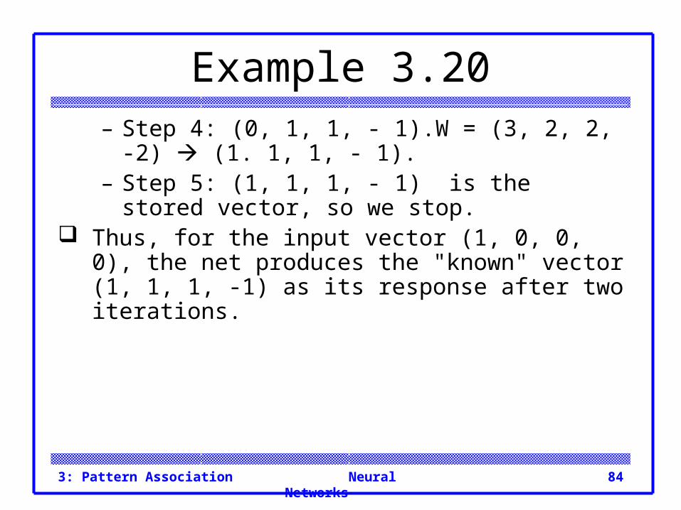
Example 3.20– Step 4: (0, 1, 1, - 1).W = (3, 2, 2, -2) (1. 1, 1, -

1).– Step 5: (1, 1, 1, - 1) is the stored vector, so we

stop. Thus, for the input vector (1, 0, 0, 0), the net

produces the "known" vector (1, 1, 1, -1) as its response after two iterations.


Example 3.20 Second input vector, (0,1,0,0)

– Step4: (0,1,0,0).W= (1,0,1,-1).– Step 5: (1, 0, 1, -1) is not the stored vector or a

previous activation vector, so we iterate.– Step 4: (1, 0, 1, -1)-W = (2, 3,2, -2) (1, 1, 1, -

1).– Step 5: (1, 1, 1, -1) is the stored vector, so we

stop. As with the first testing input, the net recognizes the

input vector (0, 1, 0, 0) as the "known" vector (1, 1, 1, -1).


Example 3.20 Third input vector, (0,0,1,0)

– Step4: (0,0,1,0).W=(1,1,0,-1).– Step 5: (1, 1, 0, -1) is neither the stored vector

nor a previous activation vector, so we iterate.– Step 4: (1, 1, 0, -1l.W = (2, 2, 3, -2) (1, 1, 1, -


stop. Again, the input vector, (0, 0, 1, 0), produces the

"known" vector (1, 1, 1, -1).


Example 3.20 Fourth input vector, (0,0,0, -1)

– Step 4: (0,0,0, -1).W = (1, 1, 1,0)– Step 5: Iterate.– Step 4: (1, 1, 1, 0).W = (2, 2, 2, -3) + (1, 1, 1, , -


stop.


Example 3.21 Testing a recurrent autoassociative net: mistakes in

the first and second components of the stored vector.

stored vector is (1, 1, 1, -1) with mistakes in two components (the first and second) is (-1, -1, 1, -1).

The performance of the net (with the weight matrix given in Example 3.20) is as follows.


Example 3.21 For input vector (-1, -1, 1, -1).

– Step 4: (-1, -1, 1, -1).W = (1, 1, -1, 1).– Step 5: Iterate.– Step 4: (1, 1, -1, 1).W = (-1, -1, 1, -1).– Step 5: Since this is the input vector repeated,

stop.


Example 3.21 (Further iterations would simply alternate the two

activation vectors produced already.) The behavior of the net in this case is called a fixed-

point cycle of length two. It has been proved that such a cycle occurs

whenever the input vector is orthogonal to all of the stored vectors in the.

The vector (- 1, - 1, 1, - 1) is orthogonal to the stored vector (1, 1, 1, - 1).

In general, for a bipolar vector with 2k components, mistakes in k components will produce a vector that is orthogonal to the original vector.


Discrete Hopfield Net An iterative autoassociative net similar to the nets

described in this chapter has been developed by Hopfield (1982, 1984).

The net is a fully interconnected neural net, in the sense that each unit is connected to every other unit.

The net has symmetric weights with no self-connections, i.e.,


Discrete Hopfield Net There are two small differences between this net

and the iterative autoassociative net: 1. only one unit updates its activation at a time

(based on the signal it receives from each other unit) and

2. each unit continues to receive an external signal in addition to the signal from the other units in the net.

The asynchronous updating of the units allows a function, known as an energy or Lyapunov function, to be found for the net.


Discrete Hopfield Net The existence of such a function enables us to prove

that the net will converge to a stable set of activations, rather than oscillating (Example 3.21).


Architecture


Algorithm


Application


Example 3.22 Testing a discrete Hopfield net: mistakes in the first

and second components of the stored vector. Consider again Example 3.21, in which the vector (1,

1, 1,0) (or its bipolar equivalent (1, 1, 1, - 1)) was stored in a net.

The units update their activations in a random order. For this example the update order is Y1 , Y4, Y3, Y2.


Example 3.22


BAM Bidirectional Associative Memory (BAM). A bidirectional associative memory stores a set of

pattern associations by summing bipolar correlation matrices (an n by m outer product matrix for each pattern to be stored).

The architecture of the net consists of two layers of neurons, connected by directional weighted connection paths.

The net iterates, sending signals back and forth between the two layers until all neurons reach equilibrium (i.e., until each neuron's activation remains constant for several steps).


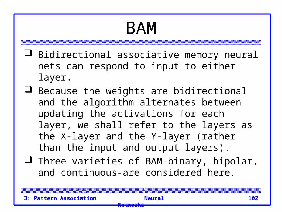
BAM Bidirectional associative memory neural nets can

respond to input to either layer. Because the weights are bidirectional and the

algorithm alternates between updating the activations for each layer, we shall refer to the layers as the X-layer and the Y-layer (rather than the input and output layers).

Three varieties of BAM-binary, bipolar, and continuous-are considered here.


Architecture


Algorithm The two bivalent (binary or bipolar) forms of BAM

are closely related. In each, the weights are found from the sum of the

outer products of the bipolar form of the training vector pairs.

Also, the activation function is a step function, with the possibility of a nonzero threshold.


Algorithm For binary patterns:

For bipolar patterns:


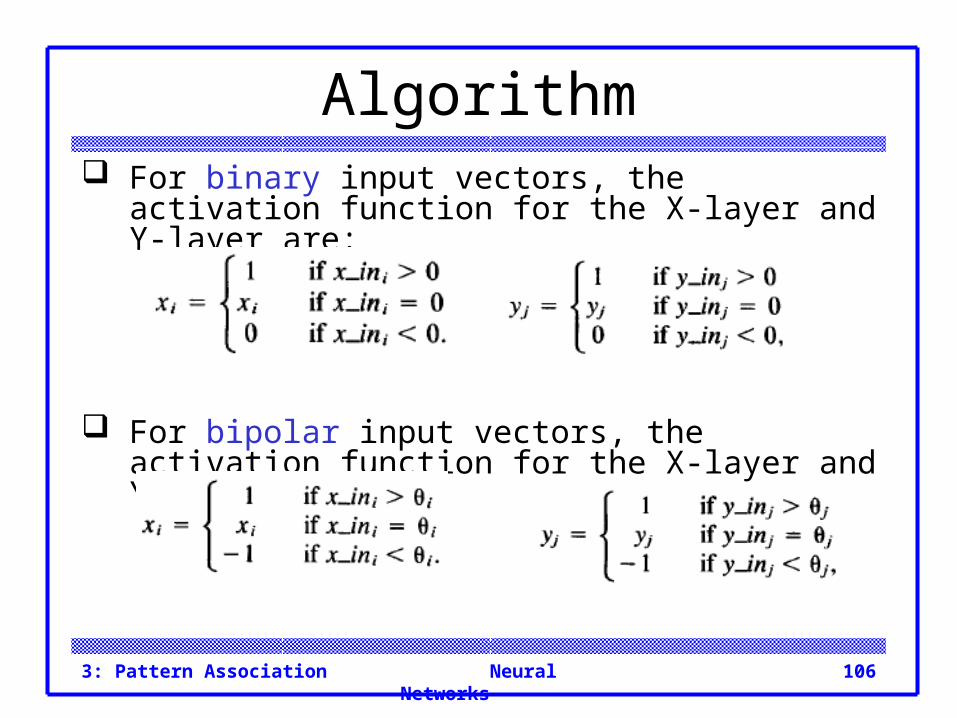
Algorithm For binary input vectors, the activation function for

the X-layer and Y-layer are:

For bipolar input vectors, the activation function for the X-layer and Y-layer are:


Algorithm The algorithm is written for the first signal to be sent

from the X-layer to the Y-layer. Signals are sent only from one layer to the other at

any step of the process, not simultaneously in both directions.


Algorithm


Continuous BAM A continuous bidirectional associative memory

transforms input smoothly and continuously into output in the range [0, 1] using the logistic sigmoid function as the activation function for all units.

For binary input vectors (s(p), t ( p ) ) , p = 1, 2, . . . , P, the weights are determined by the aforementioned formula:

The activation function is the logistic sigmoid:


Example 3.23 A BAM net to associate letters with simple bipolar

codes. Consider the possibility of using a (discrete) BAM

network (with bipolar vectors) to map two simple letters (given by 5 x 3 patterns) to the following bipolar codes:


Example 3.23


Example 3.24 Testing a BAM net with noisy input. In this example, the net is given a y vector as input

that is a noisy version of one of the training y vectors and no information about the corresponding x vector (i.e., the x vector is identically 0).


Example 3.24 This x vector is then sent back to the Y-layer, using

the weight matrix W:


Example 3.24 This result is not too surprising, since the net had no

information to give it a preference for either A or C. The net has converged to a spurious stable state, i.e., the solution is not one of the stored pattern pairs.

If, on the other hand, the net was given both the input vector y, as before, and some information about the vector x, for example,


Example 3.24 the net would be able to reach a stable set of

activations corresponding to one of the stored pattern pairs.

Note that the x vector is a noisy version of:

where the nonzero components are those that distinguish A from C:


Example 3.24


Example 3.24 Since this example is fairly extreme, i.e., every

component that distinguishes A from C was given an input value for A, let us try something with less information given concerning x.

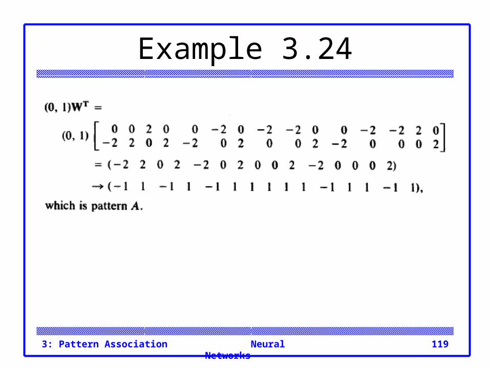
For example, let y = (0 1) and x = (0 0 - 1 0 0 1 0 1 0 0 0 0 0 0 0). Then


Example 3.24 which is not quite pattern A. So we try iterating, sending the x vector back to the

Y-layer using the weight matrix W:


Example 3.24 If this pattern is fed back to the X-layer one more

time, the pattern A will be produced.


Hamming distance The number of different bits in two binary or bipolar

vectors XI and x2 is called the Hamming distance between the vectors and is denoted by H[x1, x2].

The average Hamming distance between the vectors is 1/n.H[x1, X2], where n is the number of components in each vector.


Hamming distance The x vectors

differ in the 3rd, 6th, 8th, 9th, 12th, 13th, and 14th positions.

This gives an average Hamming distance between these vectors of 7/15. The average Hamming distance between the corresponding y vectors is 1/2.


Hamming distance Kosko (1988) has observed that "correlation

encoding" (as is used in the BAM neural net) is improved to the extent that the average Hamming distance between pairs of input patterns is comparable to the average Hamming distance between the corresponding pairs of output patterns.

If that is the case, input patterns that are separated by a small Hamming distance are mapped to output vectors that are also so separated, while input vectors that are separated by a large Hamming distance go to correspondingly distant (dissimilar) output patterns.


Erasing a stored association

The complement of a bipolar vector x is denoted xc ; it is the vector formed by changing all of the 1's in vector x to - 1's and vice versa.

Encoding (storing the pattern pair) sc: tc stores the same information as encoding s: t; encoding sc: t or s:tc will erase the encoding of s: t.


Storage capacity Although the upper bound on the memory capacity

of the BAM is min (n, m), where n is the number of X-layer units and m is the number of Y-layer units, Haines and Hecht-Nielsen [I988] have shown that this can be extended to min (2n:2m) if an appropriate nonzero threshold value is chosen for each unit.


BAM and Hopfield The discrete Hopfield net and the BAM net are

closely related. The Hopfield net can be viewed as an

autoassociative BAM with the X-layer and Y-layer treated as a single layer (because the training vectors for the two layers are identical) and the diagonal of the symmetric weight matrix set to zero.

On the other hand, the BAM can be viewed as a special case of a Hopfield net which contains all of the X- and Y-layer neurons, but with no interconnections between two X-layer neurons or between two Y-layer neurons.


BAM and Hopfield This requires all X-layer neurons to update their

activations before any of the Y-layer neurons update theirs; then all Y field neurons update before the next round of X-layer updates.

The updates of the neurons within the X-layer or within the Y-layer can be done at the same time because a change in the activation of an X-layer neuron does not affect the net input to any other X-layer unit and similarly for the Y layer units.

neural networks pattern association chapter 3. neural networks3: pattern association2 pattern...

Documents