Neural Networks for Epidemic ModellingAlan Reyes-FigueroaModelación Epidemiológica, CIMAT 12.noviembre.2020

Table of Contents

1. Introduction to Neural Networks- Crash course on neural networks- Implement fully connected networks on Keras

2. Epidemic Modelling- Fully connected neural networks- Trying to estimate parameters

3. More advanced models- Recurrent neural networks (LSTM, GRE)- Bayesian neural networks

Introduction to Neural Networks

Crash course on Neural NetworksNeural networks are mathematical / computational models inspired in how the neuronsconnect each other in the brain.The beginnings: (1940’s-1960’s)• (1943). McCulloch-Pitts neuron model, proposed by

Warren S. McCulloch, a neuroscientist, and Walter Pitts,a logician.

• (Late 40’s). Other precursors of neural networks:”Threshold Logic” – converting continuous input todiscrete output; and ”Hebbian Learning” – a model oflearning based on neural plasticity, proposed by DonaldHebb. First Hebbian networks implemented at MIT in1954.

• (1958). Frank Rosenblatt, a psychologist at Cornell,proposed the Perceptron, modelen on theMcCulloch-Pitts neuron. The Mark I Perceptron.

Crash course on neural networksThe beginnings: (1940’s-1960’s)• (1959). Bernard Widrow and Marcian Ho�, atf Stanford, developed models ADALINE

and MADALINE. (Multiple) ADAptive LINear Elements. MADALINE was the first neuralnetwork to be applied to a real-world problem. It is an adaptive filter whicheliminates echoes on phone lines. This neural network is still in commercial use.

• (Late 59’s). Marvin Minsky and Seymour Papert published the book Perceptrons.They proved the perceptron model to be limited. Mayor drawbacks and hiatus.

The XOR problem.

Crash course on neural networksResurgence: (1980’s-1990’s)• (1982). John Hopfield presented a paper to the national Academy of Sciences. His

approach to create useful devices.• (1982). US-Japan Joint Conference on Cooperative/ Competitive Neural Networks.

Funding was flowing once again.• (1985). IEEE first International Conference on Neural Networks.• (1986). Rumelhart, Hinton and Williams rediscover the backpropagation method.• (1992). Belief neural networks and statistical graphical models.• (1997). Long Short-Term Memory (LSTM) was proposed by Schmidhuber Hochreiter.• (1998). Yann LeCun published Gradient-Based Learning Applied to Document

Recognition. Start of the field applied to vision.• (1990’s). Limitations of backpropagation method. Exploding or vanishing gradient

problem.• (2000’s). Neural networks surpassed by other popular methods: SVMs and Random

Forests. Second hiatus.

Crash course on neural networksDecade of Deep Learning: (2010’s–)• (2010–). Development of modern

computation technologies: Morepowerful PC’s, development of GPU’s.

• (2012). ImageNet competition. Firstmassive neural architectures, e.g.AlexNet.

• (2015–). Deep learning tsunami.More information at• https://www.skynettoday.com/overviews/neural-net-history

• https://cs231n.github.io/neural-networks-1/

A multilayer perceptron.

Alexnet, 2014.

Neural NetworksThe area of Neural Networks has originally been primarily inspired by the goal ofmodeling biological neural systems, but has since diverged and become a matter ofengineering and achieving good results in Machine Learning tasks.

Biological motivation and connections: The basic computational unit of the brain is aneuron. Approximately 86 billion neurons can be found in the human nervous systemand they are connected with approximately 1014 − 1015 synapses.

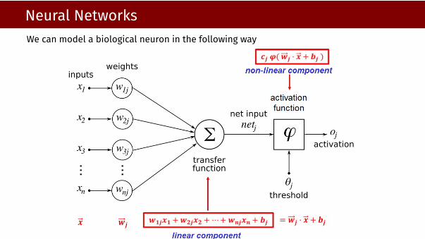
Neural NetworksWe can model a biological neuron in the following way

Neural NetworksEach neuron receives input signals from its dendrites and produces output signals alongits (single) axon. The axon eventually branches out and connects via synapses todendrites of other neurons. In the computational model of a neuron, the signals thattravel along the axons (e.g. x) interact multiplicatively (e.g. wT

j x) with the dendrites ofthe other neuron based on the synaptic strength at that synapse (e.g. wj). The idea isthat the synaptic strengths (the weights wij) are learnable and control the strength ofinfluence (and its direction: excitory (positive weight) or inhibitory (negative weight)) ofone neuron on another. In the basic model, the dendrites carry the signal to the cellbody where they all get summed. If the final sum is above a certain threshold, theneuron can fire, sending a spike along its axon. In the computational model, we assumethat the precise timings of the spikes do not matter, and that only the frequency of thefiring communicates information. Based on this rate code interpretation, we model thefiring rate of the neuron with an activation function ϕ, which represents the frequency ofthe spikes along the axon. Historically, a common choice of activation function is thesigmoid function σ, since it takes a real-valued input (the signal strength after the sum)and squashes it to range between 0 and 1.

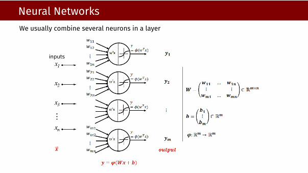
Neural NetworksWe usually combine several neurons in a layer

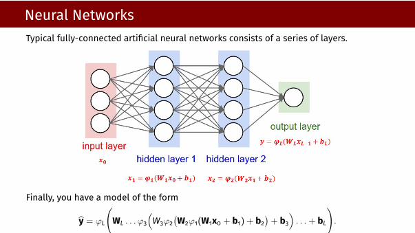
Neural NetworksTypical fully-connected artificial neural networks consists of a series of layers.

Finally, you have a model of the form

y = ϕL

(WL . . . ϕ3

(W3ϕ2

(W2ϕ1(W1x0 + b1) + b2

)+ b3

). . .+ bL

).

Deep Neural NetworksIn the era of deep learning, neural networks are specialized and specifically designed:• Convolutional neural networks: Are useful for image processing and computer

vision tasks. They use a specialized units called Convolutional Layers.

• Recurrent neural networks: Are useful for image treating sequencial data (e.g. text,time series, speech). They use a specialized repetitive units as LSTM or GRU.

Deep Neural NetworksIn the era of deep learning, neural networks are specialized and specifically designed:• Convolutional neural networks: Are useful for image processing and computer

vision tasks. They use a specialized units called Convolutional Layers.

• Recurrent neural networks: Are useful for image treating sequencial data (e.g. text,time series, speech). They use a specialized repetitive units as LSTM or GRU.

Deep Neural Networks• Graph neural networks: Are useful for processing connected structures as graphs or

networks.

• Bayesian neural networks: They try to produce not single weights, but probabilitydistributions of weights for each neuron. Useful for bayesian analysis.

Deep Neural Networks• Graph neural networks: Are useful for processing connected structures as graphs or

networks.

• Bayesian neural networks: They try to produce not single weights, but probabilitydistributions of weights for each neuron. Useful for bayesian analysis.

Activation FunctionsSome of the most common activation functions are

Activation FunctionsToday, the most used activation function is the so-called ReLU (Rectified Linear Unit). Ithas useful convergence properties.

Obs: The activation function of the output layer must be set depending on the problemobjective, or the purpose of the neural network. For example, in a classificationproblem, common activation functions are the sigmoid (binary classification) or thesoft-max (multi-classification). In a regression problem, usually one defines the linearactivation function (no activation).

ParametersThe weights WL = (wij)`, and the biases b`, ` = 1, . . . , L are the learnable parameters ofthe model. This means that we will develop an automated way to compute the weightsto ”learn” an specific task. This automated mechanism come in the way of anoptimization algorithm.Neural networks can bee seen in two di�erent forms:• As classifiers. Suppose we want to solve a classification problem (we have data,

each corresponding to a one of k di�erent labels. I this case, usually one has kneurons in the last layer (output layer) of the network. Each of this neurons,encodes the probability of the data being in each class

yi = output at neuron i = P(x is in the class i).

• As function approximators. Suppose we want to solve a regression of fittingproblem (we want to approximate a function y = f (x)). I this case, usually one has dneurons in the last layer, where y ∈ Rd. Each of this neurons, encodes theapproximation of the data y at the i−th dimensional component

yi = output at neuron i, and y = (y1, . . . , yd) is the approximation of y.

Learn by examplesNeural networks are supervised machine learning models. This means they learn byexamples. That means the following.

Suppose we have a sample of data{(xi), yi)

}ni=1. Here the xi ∈ Rp are the input data,

while the yi ∈ Rd are the ”desired” data (the ground-truth). For each i = 1, 2, . . . ,n, theneural network will produce an approximation (this is what we want) of each yi. We willdenote yi the output of the neural network when we input xi, respectively.

Learn by examplesNeural networks are supervised machine learning models. This means they learn byexamples. That means the following.

Suppose we have a sample of data{(xi), yi)

}ni=1. Here the xi ∈ Rp are the input data,

while the yi ∈ Rd are the ”desired” data (the ground-truth). For each i = 1, 2, . . . ,n, theneural network will produce an approximation (this is what we want) of each yi. We willdenote yi the output of the neural network when we input xi, respectively.

Learn by examplesNeural networks are supervised machine learning models. This means they learn byexamples. That means the following.

Suppose we have a sample of data{(xi), yi)

}ni=1. Here the xi ∈ Rp are the input data,

while the yi ∈ Rd are the ”desired” data (the ground-truth). For each i = 1, 2, . . . ,n, theneural network will produce an approximation (this is what we want) of each yi. We willdenote yi the output of the neural network when we input xi, respectively.

Thus, a neural network can be seen as an approximation f : xi → yi of the functionf : xi → yi.

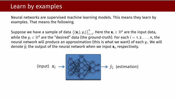
Learn by examplesNeural networks are supervised machine learning models. This means they learn byexamples. That means the following.

Suppose we have a sample of data{(xi), yi)

}ni=1. Here the xi ∈ Rp are the input data,

while the yi ∈ Rd are the ”desired” data (the ground-truth). For each i = 1, 2, . . . ,n, theneural network will produce an approximation (this is what we want) of each yi. We willdenote yi the output of the neural network when we input xi, respectively.

Thus, a neural network can be seen as an approximation f : xi → yi of the functionf : xi → yi.

Loss functionThe loss function is the objective function that describes the di�erence between theapproximations yi and the ground-truths yi, of the given sample. It will measure theerror of the discrepancy between each pair (yi, yi).

• Classification: In a classification problem, one common way to measure thedi�erence between probability values is the binary-crossentropy

L(xi, yi) = −n∑i=1

yi log(yi) + (1− yi) log(1− yi).

(if we have only two labels) or the categorical-crossentropy for a multi-labelclassification

L(xi, yi) = −n∑i=1

labels∑j=1

yij log(yij).

Loss function• Regression: In a regression problem, common ways to measure the di�erence

between the estimation yi and the desired ground-truth yi are the MSE

L(xi, yi) = MSE =1n

n∑i=1

||yi − yi||22,

and MAE errors

L(xi, yi) = MAE =1n

n∑i=1

||yi − yi||1.

Sometimes, the loss function also incorporates some regularizationterms, depending on the problem and user preferences. For example

L(xi, yi) =1n

n∑i=1

||yi − yi||1 + λ1∑i,j

||wij||1 + λ2||∇wyi||22.

BackpropagationBackpropagation is the mechanism that is used to compute the parameters of theneural network (weights wij` and biases bi`) from the loss function.

From a mathematical point of view, this is simply to compute the derivatives∇wij`L(x, y) and ∇bj`L(x, y),

for each parameter wij` and biases bi`.

Backpropagation• In the forward step, given the actual weights wij` in the network, each input xi is

passed trough the network (in fact all xi are passed at the same time), and wecompute te estimations yi. Then, the los function L is computed.

• In the backward step, we compute the derivatives ∇wij`L and ∇bj`L. Then theweights wij` and biases bi` are recalculated.

• Both steps are repeated until we reach convergence, or some other stop criterionholds.

The re-calculation process is done by using the gradient descent optimization algorithm,

w(k+1)ij` = w(k)

ij` − α∇w(k)ij`L(x, y),

b(k+1)i` = b(k)i` − α∇b(k)i`

L(x, y),

Here, α > 0 is the step size of learning rate. In practice, today we use any of thestochastic variants of gradient descent.

Backpropagation Example

Backpropagation Example

Stochastic gradient descent• Classic gradient descent: It computes the loss function L from all samplesx1, . . . , xn, and then actualize the weights.

• Stochastic gradient descent: At each iteration, it randomly chooses one sample xi(with equal probability and no replacement), it computes the loss L using only thesample xi, and then actualize the weights. This is repeated until all the sampleswere chosen. After all samples are used, we complete one epoch.

• Mini-batch gradient descent: We split the sample in b subsets or batches B1, . . . ,Bb.At each iteration, it randomly chooses one batch Bj (with equal probability and noreplacement), it computes the loss L using only the samples in batch Bj, and thenactualize the weights. This is repeated until all batches are chosen. After allsamples are used, we complete one epoch.

There are a lot of variants and improvements of stochastic gradient descent. Seehttps://ruder.io/optimizing-gradient-descent/

Optimization process

Di�erences between gradient descent and stochastic gradient descent: (a) gradient de-scent. (b) Stochastic gradient descent.

In summaryParameters: (learnable by gradient descent)• weights wij` and biases bi`, for ` = 1, . . . , L.

Hyper-parameters: (user-defined, non-learnable by gradient descent)• Number of layers, and the type of each layer.• Size of each layer (number of neurons in each layer).• Activation function of each layer.• Connections between the layers.

• Loss function (and other metrics).• Optimization algorithms (GD, SGD, Nesterov, Adam, Adagrad, Adamax, RMSProp, ...),

and parameters of those algorithms.• learning rate or step-size α.• Size ob the batch.• Number of epochs.

• Training / Validation / Test partition size ...

Train / Validation / TestTo evaluate the performance of our neural network model, and evaluate the trainingprocess, we usually split our data in two (or three) subsets: training data, validationdata, test data.• Training data: used for the training process, this is the sample to compute loss

function and weights.• Validation data: used also in the training process, but just to evaluate the loss with

new data. They are not used to compute the weights.• Test data: used at the end for the final evaluation of the performance. Typically

used to report performance in papers.

EvaluationThere is no a recipe for the size or percentage of each subset. Common values are:Training (80%), Validation (10%), Test (10%),Training (60%), Validation (20%), Test (20%),Training (50%), Validation (40%), Test (10%),Depends on how much data you have, how much data you can sacrifice for testing, ...

We want to evaluate our model to see if it generalizes well new unseen samples(bias-variance trading).

EvaluationThere is no a recipe for the size or percentage of each subset. Common values are:Training (80%), Validation (10%), Test (10%),Training (60%), Validation (20%), Test (20%),Training (50%), Validation (40%), Test (10%),Depends on how much data you have, how much data you can sacrifice for testing, ...

We want to evaluate our model to see if it generalizes well new unseen samples(bias-variance trading).

Evaluation

Training/validation learning curves. The ideal case is the red curve.

Evaluation

Examples of training/validation learning curves

Evaluation

Other useful insights from the learning curves.

Implement neural networks inKeras

Libraries for deep learningThere are a lot of libraries and online resources to do deep learning.

Libraries for deep learningThe most popular are

Keras documentation: https://keras.io/api/

KerasKeras was created by Francois Chollet (2015-2016), while working at Google. It began asan independent library, but today comes as a module inside Tensorflow.

Books by F. Chollet. (2018). Deep Learning with Python. Deep Learning with Python. Manning.

Other ReferencesManning and O’Reilly are editorial with good practical books on deep learning, andmachine learning in general (as well as other computational resources).

Other ReferencesThere are few (serious) books on deep learning. The most part of material comes in theform of papers. In the web there are a lot of resources in form of blogs and tutorials.

Objectives for Practical Session 1• Implement a fully-connected neural network on Keras, suitable for a regression

problem.

• Learn how to prepare the data ready for input the neural network.• Learn how to define the optimization algorithm.• Learn how to define the loss function and evaluation metrics.• Learn how to set some hyper-parameters: (learning rate, batch size, stop criteria).

• Fitting the model.• Learn how to plot learning curves, and get useful information of the model from

them.• Learn how to predict from new data.• Evaluate the performance on new data.