neural network modeling and an uncertainty analysis in...
TRANSCRIPT

Neural network modeling and an uncertainty analysisin Bayesian framework: A case study from the KTBborehole site
Saumen Maiti1 and Ram Krishna Tiwari2
Received 11 January 2010; revised 5 June 2010; accepted 25 June 2010; published 26 October 2010.
[1] A new probabilistic approach based on the concept of Bayesian neural network (BNN)learning theory is proposed for decoding litho‐facies boundaries from well‐log data.We show that how a multi‐layer‐perceptron neural network model can be employedin Bayesian framework to classify changes in litho‐log successions. The method isthen applied to the German Continental Deep Drilling Program (KTB) well‐log datafor classification and uncertainty estimation in the litho‐facies boundaries. In thisframework, a posteriori distribution of network parameter is estimated via the principleof Bayesian probabilistic theory, and an objective function is minimized following thescaled conjugate gradient optimization scheme. For the model development, we inflicta suitable criterion, which provides probabilistic information by emulating differentcombinations of synthetic data. Uncertainty in the relationship between the data and themodel space is appropriately taken care by assuming a Gaussian a priori distributionof networks parameters (e.g., synaptic weights and biases). Prior to applying the newmethod to the real KTB data, we tested the proposed method on synthetic examples toexamine the sensitivity of neural network hyperparameters in prediction. Within thisframework, we examine stability and efficiency of this new probabilistic approach usingdifferent kinds of synthetic data assorted with different level of correlated noise. Ourdata analysis suggests that the designed network topology based on the Bayesian paradigmis steady up to nearly 40% correlated noise; however, adding more noise (∼50% or more)degrades the results. We perform uncertainty analyses on training, validation, and testdata sets with and devoid of intrinsic noise by making the Gaussian approximation of the aposteriori distribution about the peak model. We present a standard deviation error‐map atthe network output corresponding to the three types of the litho‐facies present over theentire litho‐section of the KTB. The comparisons of maximum a posteriori geologicalsections constructed here, based on the maximum a posteriori probability distribution,with the available geological information and the existing geophysical findings suggestthat the BNN results reveal some additional finer details in the KTB borehole data atcertain depths, which appears to be of some geological significance. We also demonstratethat the proposed BNN approach is superior to the conventional artificial neural networkin terms of both avoiding “over‐fitting” and aiding uncertainty estimation, which arevital for meaningful interpretation of geophysical records. Our analyses demonstratethat the BNN‐based approach renders a robust means for the classification of complexchanges in the litho‐facies successions and thus could provide a useful guide forunderstanding the crustal inhomogeneity and the structural discontinuity in manyother tectonically complex regions.
Citation: Maiti, S., and R. K. Tiwari (2010), Neural network modeling and an uncertainty analysis in Bayesian framework:A case study from the KTB borehole site, J. Geophys. Res., 115, B10208, doi:10.1029/2010JB000864.
1. Introduction
[2] Litho‐facies classification based on experimental datais one of the important problems in geophysical well‐logstudies. Since permeability and fluid saturation for a givenporosity varies considerably among the litho‐facies at a
1Indian Institute of Geomagnetism, Navi‐Mumbai, India.2National Geophysical Research Institute, Hyderabad, India.
Copyright 2010 by the American Geophysical Union.0148‐0227/10/2010JB000864
JOURNAL OF GEOPHYSICAL RESEARCH, VOL. 115, B10208, doi:10.1029/2010JB000864, 2010
B10208 1 of 28

certain depths, classification of litho‐facies and their ade-quate representation in a 3‐D cellular geophysical/geologicalmodel is vital for understanding the crustal inhomogeneity,the permeability, and the fluid saturation for exploration ofoil and gas. The best sources of litho‐facies informationare core samples of reservoir rocks collected from wells.However, cores are not commonly taken due to high costs.The availability of core samples is also limited in comparisonto the number of drilled wells in the geological/geophysicalfield. Hence, in a situation where core information is notavailable, the down‐hole geophysical logs can be used as analternative to infer the nature of surrounding rocks/lithology[Benaouda et al., 1999].[3] During the past decades, several researchers have
attempted to solve the problems of litho‐facies classificationusing conventional methods like, graphical cross‐plottingand multivariate statistical analyses [Rogers et al., 1992]. Inthe graphical cross‐plotting technique [Pickett 1963; Gassawayet al., 1989], two or more well‐logs data are cross‐plotted toyield lithologies. Multivariate statistical methods such as“principle component” and “cluster analysis” [Busch et al.,1987; Wolff and Pelissier‐Combescure, 1982] and “dis-criminant function analysis” [Delfiner et al., 1987] have alsoinvariably been used for the interpretation of borehole data.These techniques are, however, semi‐automatic and require alarge amount of data, which is costly and not easily available.Further the existing methods are also very tedious and time‐consuming, particularly when it deals with the large numberof noisy and complex borehole data.[4] Appropriate mathematical modeling and statistical
techniques can be applied to extract the meaningful infor-mation about the subsurface properties of the real earth (e.g.,lithology, porosity, density, hydraulic conductivity, resis-tivity, salinity, water/oil saturation, etc.) using surface and/or borehole measurements [Aristodemou et al., 2005]. Inorder to convalesce the model parameters correctly, an errorfunction, which is a measure of discrepancy between theobservables and the predictions from a forward‐modelingcalculation, is minimized [Mosegaard and Tarantola, 1995;Tarantola, 1987, 2006; Devilee et al., 1999; Bosch, 1999;Bosch et al., 2001; Aristodemou et al., 2005; Meier et al.,2007]. However, well‐log signals, which are a proxy oflithology/litho‐facies, are essentially the result of complexnonlinear geophysical processes arising primarily due to thevariability and interactions of several factors, such as porefluid, effective pressure, fluid saturation, pore shape, andgrain size. Further, the well‐log records are often found tobe contaminated with inescapable correlated red noise pri-marily due to the deplorable borehole conditions. Therefore,estimation of lithology/litho‐facies from well‐log signalsessentially constitutes a nonlinear geophysical inverseproblem.[5] In the recent past, artificial neural network (ANN)‐based
techniques have been extensively applied to solve nonlinearproblems in almost all branches of geophysics [Van der Baanand Jutten, 2000; Poulton, 2001]. Examples include (1) seis-mic event classification [Dystart and Pulli, 1990; Dai andMacBeth, 1995], (2) well‐log analysis [Baldwin et al., 1990;Rogers et al., 1992; Helle et al., 2001; Aristodemou et al.,2005; Maiti et al., 2007; Maiti and Tiwari, 2009], (3) firstarrival picking [Murat and Rudman, 1992;McCormack et al.,1993], (4) earthquake time series modeling [Feng et al.,
1997], (5) inversion [Raiche, 1991; Roth and Tarantola,1994; Devilee et al., 1999; Meier et al., 2007], (6) param-eter estimation in geophysics [Calderon‐Macias et al.,2000], (7) prediction of aquifer water level [Coppolaet al., 2005], (8) magneto‐telluric data inversion [Spichakand Popova, 2000], (9) magnetic interpretations [Bescobyet al., 2006], and (10) signal discrimination [Maiti andTiwari, 2010]. This type of network, however, does yieldmean solutions to the inverse problem whose solution isessentially probabilistic in nature [Devilee et al., 1999]. Inaddition to this, there are several other drawbacks inconventional neural network approaches [Bishop, 1995;Coulibaly et al., 2001; Aires, 2004; Maiti and Tiwari, 2009,2010]. One of the major limitations in the conventionalANN approach is frequent appearance of local and globalminima in the modeled results. To surmount this problem,the network is trained by maximizing a likelihood functionof the parameters or equivalently minimizing an errorfunction to obtain the best set of parameters starting with aninitial random set of parameters. Sometimes a regularizationterm with an error function is also included in the process ofanalysis for preventing over‐fitting. However, in the con-ventional ANN approach, a complex model can fit trainingdata well, but it does not necessarily guarantee smaller errorsin the unseen data [Bishop 1995; Coulibaly et al., 2001].This is because the conventional ANN does not take accountof uncertainty in the estimation of parameters [Bishop 1995;Nabney, 2004].[6] Roth and Tarantola [1994] have assessed the stability
and the effectiveness of an ANN inversion scheme in thepresence of noise while inverting seismogram records torecover the crustal velocity structure. After several experi-ments, they have concluded that the ANN‐based methodsare not stable for analyzing strongly correlated noisy geo-physical signals; however, the methods could be used forsolving the nontrivial inverse problem. More recently,Devilee et al. [1999] proposed an efficient probabilisticANN‐based approach to determine the Eurasian crustalthickness from surface wave velocities data. FollowingDevilee et al. [1999], some researchers [Meier et al., 2007]have provided a similar ANN‐based approach by a mixturedensity network (MDN), which actually combines the con-cept of both histogram and median type network, to estimatethe global crustal thickness from the surface wave data.Solving the inverse problems requires precise estimation ofuncertainties to know what it means to fit the data. MacKay[1992] introduced first a fully Bayesian approach where thescalar hyperparameters of a network are estimated via theso‐called evidence program. While inverting the remote‐sensing data, Aires [2004] has given a theoretical treatmentfor ANN uncertainty estimation using the Bayesian statis-tics. This made use of the fully Bayesian concept via theevidence program. However, this approach is not tested onthe data contaminated with different levels of correlated/colored noise.[7] In the present work, we employ a newly developed
BNN probabilistic approach [Bishop, 1995; Nabney, 2004],for classification of changes in litho‐facies units from theGerman Continental Deep Drilling Project (KTB) well‐logdata. We use multiple output node histogram networks,which return probabilistic information equidistantly ongeophysical inverse problems by emulating the solution
MAITI AND TIWARI: BNN MODELING OF KTB WELL LOG DATA B10208B10208
2 of 28

from samples. The stability and effectiveness of theBayesian neural network (BNN) approach on noisy as wellas on noise‐free data are also examined. The algorithmessentially allows us to estimate uncertainty in the datamixed with or devoid of correlated/colored noises. Wecompared our results of KTB well‐log data with the existingresults from other methods. Our results suggest that theBNN technique is superior to the other conventional ANNtechniques in a sense that it takes care of the problems ofuncertainty analysis, over‐fitting and under‐fitting in anatural way even if the data are contaminated with somepercentage of noise. The comparison of regression resultsbetween the BNN and the super self adaptive back‐propa-gation (SSABP) [Maiti et al., 2007] and the result ofuncertainty analysis along the entire length of the litho‐section are quite encouraging. Thus, besides introducing anew ANN approach based on the Bayesian paradigm formodeling the international quality of well‐log data, thepresent analysis has also brought out some new results thus,exploring the generality of the method from the point ofview of the actual application in other domains.
2. About the KTB
[8] The German Continental Deep Drilling Project (KTB)explores a metamorphic complex in northeastern Bavaria,southern Germany [Maiti et al., 2007, Figure 1]. Litholog-ically, the continental crust at the drill site consists of threemain facies units: paragneisses, metabasites, and heteroge-neous series having alternations of gneiss‐amphibolites, withminor occurrence of marbles, calcsilicates, orthogeneisses,lamprophyres, and diorites [Franke, 1989; Berckhemer et al.,1997; Emmermann and Lauterjung, 1997; Pechnig et al.,1997; Leonardi and Kumpel, 1998, 1999]. The detailedinformation concerning the KTB data and its geophysicalsignificance can be found in several earlier papers [Franke,1989; Berckhemer et al., 1997; Pechnig et al., 1997;Emmermann and Lauterjung, 1997; Leonardi and Kumpel,1998, 1999]. We used here three types of well‐log data,density, neutron porosity, and gamma ray intensity for con-straining the litho‐facies boundaries for the KTB modelingstudy. Total depths of the main hole and pilot hole are 9101m and 4000 m, respectively. The borehole data are sampledat 0.15 m (6 inch) intervals [Maiti et al., 2007].[9] The rocks were metamorphosed at a pressure of 6–
8 kbar and a temperature of 650°C–700°C. This mediumgrade metamorphism took place in the Lower to middleDevonian (410–380 Ma ago) [Leonardi and Kumpel, 1998].The crustal heterogeneities at the KTB borehole site are welldocumented [Leonardi and Kumpel, 1998]. These recordsare a complete, continuous, and uninterrupted series andhence could be appropriately utilized for the classification ofthe litho‐facies units in a new perspective of Bayesian
framework. A brief summary of the data and its geophysical/geological significance pertinent to this study is, however,presented here to preserve self‐sufficiency of the paper.
2.1. Data
[10] Density data were measured using gamma raysemanating from a 137Cs source that enters the wall rocks andare backscattered to a gamma detector (Litho Density Tool,LDT). Its vertical resolution is 1 m (Table 1). Neutronporosity values too are determined by using devices withradioactive sources. For the porosity logging, neutrons areemanated from an Am‐Be radioactive source, and the rocksresponse, in the form of either gamma rays or fast neutronsor slow neutrons, is determined by an appropriate sensor(Neutron Compensated Log, NCL). For a constant boreholegeometry. the response is a measure of the concentration ofhydrogen atoms, which in the case of fluids‐saturated rocksis related to the porosity of the geological formations. TheNCL has a vertical resolution of 1 m (Table 1).[11] The gamma ray radiation was measured using a
Neutral Gamma Ray Spectrometer (NGS). This tool quan-tifies the natural gamma ray spectra of the isotopes 40K,232Th, and 238U. The bulk gamma ray intensity, deducedfrom the NGS data, is directly proportional to the concen-tration of the corresponding isotopes in a geological for-mation. The variations within a recorded log thus indicatechanges in the lithology. High concentrations of K, Th, andU in crystalline successions reveal the presence of acidicrocks such as paragneisses, whereas the basic compositionsare reflected by a scarcity of radio nuclides [Leonardi andKumpel, 1999]. The gamma intensity is measured in theconventional American Petroleum Institute (API) unit. Thevertical resolution is estimated to be 0.5 m (Table 1)[Leonardi and Kumpel, 1998].
2.2. Relationship Between the Log Responseand Regional Geology
[12] Gamma ray activity exhibits a general increase fromthe most mafic rocks (ultramafites) to the most acidic rocks(potassium‐feldspar gneisses) because of the chemicalcomposition. In the KTB crystalline metamorphic basement,the total gamma ray is the most crucial physical parameterfor differentiating the succession. In general, amphibolitesand metagabbros, which are the main rock types of themassive metabasite units, are physically characterized bylower gamma ray activity and higher density than the rocksof the paragneisses sections. This is related to the mineralcontent, which within metabasites consists of more maficand dense minerals like hornblende and garnet biotite.Paragneisses sections are composed mainly of quartz, pla-gioclase, and micas [Berckhemer et al., 1997; Emmermannand Lauterjung, 1997; Pechnig et al., 1997]. Since porespace in the crystalline basement is very low, neutron
Table 1. Showing Physical Properties, Recording Tool, and Vertical Resolution of Well Log Data Used in the Study
Physical Properties ToolVertical
Resolution Unit Principle
Bulk density Litho density tool (LDT) 1 m Grams per cubic centimeter Absorption/scattering of gamma raysNeutron porosity Compensated neutron porosity (CNT) 1 m % (limestone porosity unit) Absorption of neutronsGamma ray intensity Natural gamma ray spectrometer (NGS) 0.5 m American Petroleum Institute (API) Natural gamma ray emissions
MAITI AND TIWARI: BNN MODELING OF KTB WELL LOG DATA B10208B10208
3 of 28

porosity response is found to be dependent upon the min-eralogical composition. Enhanced porosity is, in general,restricted to discrete zones of faulting and fracturing; how-ever, neutron porosity in undisturbed depth sections is pre-dominantly reacting to the water bound minerals likephyllosilicates or amphiboles [Pechnig et al., 1997]. Hence,rock types poor in these minerals, such as quartz and feldspar‐rich gneisses show very low neutron porosities. In contrast,rocks with high phyllosilicate and amphibole contents pro-duce high values in the neutron porosity. We note thatgeneral log response knowledge is used for constructingnetwork samples.[13] The 3‐D cross plot of density (g/cc), neutron porosity
(%) and gamma ray (API) of the KTB main hole and pilothole shows the strong overlapping/superposing well‐logsignal characteristics in 3‐D parameter space (Figure 1).This overlapping signals could be characterized partly dueto the physics (amalgamated rock structure limited byresolving power of data characteristics) and partly due to thenoise (that may be of any kind, white Gaussian, red, pink,
blue, etc.) in the well‐log data. The complex nonlinearoverlapping pattern of observed well‐log data apparentlyevident in Figures 1a and 1b suggests that it may not beappropriate to apply linear inversion method to classifylitho‐facies units. It is therefore prudent to employ a non-linear inversion scheme to obtain a general probabilitydensity function (pdf) in Bayesian framework to exploreprecisely the successions of litho‐facies units.
3. Probabilistic Solution of Inverse Problem
[14] The solution to a general inverse problem can begiven in the form of a pdf, P(x, d) [Tarantola, 1987; Sen andStoffa, 1996; Bosch, 1999; Sambridge and Mosegaard,2002], where d represents a set of distinct measurementsand x is a set of model parameters. In the Bayesian frame-work, the solution can be given by
P x j dð Þ ¼ P d j xð ÞP xð ÞP dð Þ ð1Þ
Figure 1. (a) Cross plot of density (g/cc), porosity (%), and gamma ray intensity (API) of KTB pilot holeshowing strong nonlinearity and difficulty to establish parametric boundaries (b) same for KTB mainhole.
MAITI AND TIWARI: BNN MODELING OF KTB WELL LOG DATA B10208B10208
4 of 28

Where, P() stands for probability, d represents a set of dis-tinct measurements, and x is a set of model parameters.Thus, P(d∣x) represents a pdf of observed data given themodel, (likelihood); P(d) is the pdf of the data d (scale factorin version represents limitations on the data space imposedby the physics and prior constraints on the model space),and P(x) is the pdf of the model parameter x, independent ofthe data (prior information on model). The solution of theinverse problem for a specific experiment may be approxi-mated by the sampling based method according to P(x, d).But forming the solution requires too many forward calcu-lations [Devilee et al., 1999]. Instead, a neural networkproperly trained on a finite data set {d, x} can emulate theconditional pdf P(x∣d).
4. Artificial Neural Networks
[15] An artificial neural network is an abstract model ofthe brain, consisting of simple processing units—similar to“neurons” in the human brain—connected layer by layer toform a network [Rosenblatt, 1958; Meier et al., 2007]. Amulti‐layer perceptron (MLP) is a special configuration ofan ANN [Bishop, 1995] that ranges among the most pow-erful methods for solving the nonlinear classification andboundaries detection problems. The MLP model consists ofone input layer, one output layer, and at least one interme-diate hidden layer between the input and output layer. In afully connected MLP, a neuron (node) of each layer isconnected to a neuron of the next layer through a synapticweight. Output of the input layer is then fed to the input ofthe hidden layer and the output of the hidden layer is thenfed to the input of the output layer (Figure 2a). The infor-mation propagates in one direction from the input layer tothe output layer.[16] The ANN works by adapting weights and biases in
order to minimize error functions between the “networkoutput” and the “target values” via a suitable algorithm. Thepopularly known back‐propagation (BP) algorithm uses thescaled conjugate gradients (SCG) and quasi‐Newton meth-ods for optimization of synaptic weights and biases[Rumelhart et al., 1986] (Figure 2a). In our work we use anonlinear hyperbolic tan sigmoid transfer function of theform
fj net lð Þj
� �¼ e� net lð Þ
jð Þ � e�� net lð Þjð Þ
e� net lð Þjð Þ þ e�� net lð Þ
jð Þ : ð2Þ
Here, e denotes the basis of the natural logarithm (Figure 2a),and b is a constant that determines the stiffness of thefunction near
net lð Þj ¼
Xni¼1
w lð Þji d
l�1ð Þi �Q lð Þ
j ¼ 0 ð3Þ
in layer (l) [Roth and Tarantola, 1994]. netj(l) is a value
received by the jth node in layer (l ), wji(l) is a connection
weight between the ith node in layer (l − 1) and the jth nodein layer (l ), and di be an input is a variable for the ith node inlayer (l − 1). Qj
(l) is a bias unit for the jth node in layer (l ).The value of b is adopted as 1.0 to keep the transfer functionin sigmoidal shape [Roth and Tarantola, 1994]. Henceforth,it might be more convenient to put the first and second layer
synaptic weight and bias term into a single networkparameter w.[17] The principle goal of the neural network approach is
to learn the relationship between an input and an output inspace/domain from a finite data set s = {dk, xk; k = 1, ..., N}by adjusting network parameters w (weight and biases). Thisis done by maximizing the likelihood of the data set S (orequivalently by minimizing its negative logarithm), whichforms a conventional least squares error measure in the form
E ¼ 1
2
XNk
xk � ok dk ;wkð Þ2n o
; ð4Þ
where xk and ok are, respectively, the target/desired and theactual output at each node in the output layer. We note thatinput d consists of three types of well‐log data (viz. density,neutron porosity, and gamma ray intensity) and output xconsists of three types of litho‐facies present over the KTBsuper deep borehole. We construct the histogram networkintroduced by Devilee et al. [1999] which emulates theconditional pdf P(x∣d) directly to the new input d. We willreturn to that in section 4.1.
4.1. Histogram Network
[18] Devilee et al. [1999] introduced a histogram‐typenetwork which provides a finite discritization of P(x, d). Thek‐output of a histogram network emulates equidistantlysampled approximation of the solution, i.e., pdf P(x∣d).Suppose, we consider the case of a scalar x and apply thefollowing operator to discritize its value using k‐segmentswith length Dx:
xk xð Þ ¼1 kDx < x < ðk þ 1ÞDx
0 otherwise
8<: : ð5Þ
The k‐output ok (d) of the optimally trained network gives
ok dð Þ ¼Zxoþ kþ1ð ÞDx
x0þkDx
P x j dð Þdx � Pk dð Þ: ð6Þ
For each set of inputs d, the trained network has k‐outputsok (d) which return the probabilities that x takes a value in thekth window of width Dx. With k = 3, we obtain our appli-cation of classification of input into one of the three states.We note that the solution approximately satisfiesX
Pk ¼ 1: ð7Þ
4.2. Bayesian Neural Networks
[19] In a conventional neural network approach, often aregularization term is incorporated to solve equation (4) andoptimize the objective function:
E wð Þ ¼ �ES þ �ER: ð8Þ
Here l and m, which control other parameters (synapticweight and biases), are known as hyperparameters. For
ER = 12
PRi¼1
wi2, R is the total number of weights and biases in
MAITI AND TIWARI: BNN MODELING OF KTB WELL LOG DATA B10208B10208
5 of 28

Figure 2. (a) Layout of the MLP with a three layer neural networks with d representing input and sub-script i representing the number of “nodes” in the input layer. At each node of the hidden layer, the netarguments are squashing through a nonlinear activation function of type hyperbolic tangent where wji
represents the connection weight between the ith node in the input layer and the jth node in the hiddenlayer. wjk, represents the connection weight between the jth node in the hidden layer and the kth node inthe output layer; Qj and Qk are bias vectors for the hidden and the output layer. Now aj = fj(netj) is theoutput of the weighted sum through the activation function following equation (2). When the sum of theargument of a neuron is comparable to the threshold value Qj, the sigmoid function squashes linearly;otherwise, it saturates with value +1; –1 gives nonlinearity for nonlinear mapping between an input and anoutput space. (b) A simple example of the application of BNN to a “regression” problem. Here 50 datapoints have been generated by sampling the function defined by equation (25); the network consists of aMLP with five hidden units having tanh activation functions and one linear output unit/node. The“network” shows the BNN results with the weight vector set to wMLP corresponding to the maximum ofthe posterior distribution, and the “error bar” representing ±1d from equation (45). Notice how the errorbars are larger in regions of low data density. (c) Same when the standard deviation of noise distribution is0.5. (d) Example when no regularization is used and the standard deviation of noise distribution is 0.1.(e) Example when the data are sampled at point 0.25 and 0.90 and the standard deviation of noise dis-tribution is 0.1.
MAITI AND TIWARI: BNN MODELING OF KTB WELL LOG DATA B10208B10208
6 of 28

Figure 2. (continued)
MAITI AND TIWARI: BNN MODELING OF KTB WELL LOG DATA B10208B10208
7 of 28

the network. This corresponds to the use of simple weight‐decay regularizer, which gives a prior distribution of theform [Bishop, 1995] of
P wð Þ ¼ 1
QR �ð Þ exp ��
2k w k2
� �: ð9Þ
Thus, when kwk is large, ER is large, and P(w) is small, andso this choice of prior distribution says that we expect theweight values to be small rather than large. Thus, the reg-ularization term favors small values for network weight andbiases and decreases the tendency of a model to “over‐fit”noise in the training data. In the traditional approach, thetraining of a network begins by initializing a set of weightsand biases and ends up with the single best set of weightsand biases given the objective function is optimized.[20] In the Bayesian approach, a suitable prior distribu-
tion, say P(w) of weights is considered before observing thedata instead of a single set of weights. Using Bayes’ rule,one can write a posteriori probability distribution for theweights, as [Bishop , 1995; Aires , 2004; Khan andCoulibaly, 2006]
P w j sð Þ ¼ P s j wð ÞP wð ÞP sð Þ ; ð10Þ
where P(s ∣ w) is a data set likelihood function and thedenominator P(s) is a normalization factor. Integrating outover the weight space, we obtain [Bishop, 1995; Aires 2004;Nabney, 2004; Khan and Coulibaly, 2006]
P sð Þ ¼Z
P s j wð ÞP wð Þdw: ð11Þ
Equation (11) ensures that the left‐hand side of equation (10)gives unity when integrated over all the weight space. Oncethe posterior has been calculated, all types of inference areobtained by integrating out over that distribution. Therefore,implementing the Bayesian method, expressions for the priordistributions P(w) and likelihood function P(s∣w) are needed.The prior distribution P(w) can be expressed in terms of aweight decay regularizer, ER of the conventional learningmethod. For example, if a Gaussian prior is considered,we can write the distribution as an exponential of the form[Bishop, 1995; Nabney, 2004]
P wð Þ ¼ 1
QR �ð Þ exp ��ERð Þ; ð12Þ
where QR (l) is a normalization factor and can be given by[Bishop, 1995; Nabney, 2004]
QR �ð Þ ¼Z
exp ��ERð Þdw: ð13Þ
Equation (12) ensures thatRp(w)dw = 1. The hyperpara-
meter l can be fixed or could be optimized as part of thetraining process [Nabney, 2004]. Note that in practice it isdifficult to know the prior state of information about thenetwork weight in advance. It is the Bayesian machineryemployed to provide a neat, tractable, and sound mathe-matical framework to update the network parameter distri-
bution. Here a Gaussian prior is chosen because it simplifiesthe calculation of the normalization coefficient QR (l) usingequation (13) giving [Bishop, 1995; Nabney, 2004]
QR �ð Þ ¼ 2�
�
� �R=2
: ð14Þ
[21] Alternative choices for the prior P(w) have beendiscussed in great length by Buntine and Weigend [1991],Neal [1993], and Williams [1995]. The data‐dependentlikelihood function in Bayes’ theorem can be formed interms of the error function, ES of the conventional method.For instance, if the noise (error) model is Gaussian, anequation we write for likelihood function is [Bishop, 1995;Aires, 2004; Nabney, 2004; Khan and Coulibaly, 2006]
P s jwð Þ ¼ 1
QS �ð Þ exp ��ESð Þ: ð15Þ
The function QS (m) is a normalization factor given by
QS �ð Þ ¼Z
exp ��ESð Þds; ð16Þ
whereRds =
Rdx1…dxN represent integration out over the
target variables. If it is assumed that the target data aregenerated from a smooth function with additive zero meanGaussian noise, the probability of observing the data value xfor a given input vector d would be
P x j d;wð Þ / exp ��
2x� o d;wð Þf g2
� �; ð17Þ
where o(d; w) represents a network function governing themean of the distributions, w denotes the correspondingweight vector, and the parameter m controls the variance ofthe noise. Provided the data points are drawn independentlyfrom this distribution, we have the expression for the like-lihood as [Bishop, 1995; Aires, 2004; Khan and Coulibaly,2006]
P s j wð Þ ¼YNk¼1
P xk j dk ;wð Þ ¼ 1
QS �ð Þ exp ��
2
XNk¼1
xk � ok dk ;wð Þf g2 !
:
ð18Þ
The expression in equation (16) for the normalization factorQS (m) is then the product of N independent Gaussianintegrals, which have been evaluated by Bishop [1995].Accordingly, we can write
QS �ð Þ ¼ 2�
�
� �N=2
: ð19Þ
After deriving the expressions for prior and likelihoodfunctions and the posterior distribution of weights and usingthose expressions in equation (10), we obtain [Bishop, 1995;Aires, 2004; Khan and Coulibaly, 2006]
P w j sð Þ ¼ 1
QEexp ��ES � �ERð Þ ¼ 1
QEexp �E wð Þð Þ; ð20Þ
MAITI AND TIWARI: BNN MODELING OF KTB WELL LOG DATA B10208B10208
8 of 28
where
E wð Þ ¼ �ES þ �ER ¼ �
2
XNk¼1
xk � ok dk ;wð Þf g2þ�
2
XRi¼1
w2i ð21Þ
and
QE �; �ð Þ ¼Z
exp ��ES � �ERð Þdw: ð22Þ
In equation (20), the objective function in the Bayesianmethod corresponds to the inference from the posteriordistributions of the network parameters w. After defining theposterior distributions, the network is trained with a suit-able optimization algorithm to minimize the error functionE(w) or equivalently to maximize the posterior distributionP(w∣s). Using the rules of conditional probability, the dis-tribution of outputs for a given input vector, d, we can writein the form of [Bishop, 1995; Aires, 2004; Khan andCoulibaly, 2006]
P x j d; sð Þ ¼Z
P x j d;wð ÞP w j sð Þdw: ð23Þ
We note that P(x ∣ d, w) is simply the model for distributionof noise on the target data for a fixed value of weight vectorwMLP and can be expressed by equation (17), and P(w ∣ s) isthe posterior probability distribution of weight. If the data setis large, the posterior distribution P(w ∣ s) may be approxi-mated to Gaussian distribution [Walker, 1969]. After somesimplification, we can write the integral of equation (23) as[Bishop, 1995]
P x j d; sð Þ ¼ 1
2��2ið Þ1=2exp � x� o d;wMLPð Þðf g2
2�2i
!; ð24Þ
whose mean is o(d; wMLP), and variance is given by [Bishop,1995]
�2i ¼1
�þ gTH�1g: ð25Þ
Here, m is a hyperparameter and is actually the inverse vari-ance of the noise model, and g denotes the gradient of o(d; w)with respect to the weights w evaluated at wMLP and H is theHessian matrix of the total(regularized) error function withelements, which we can write [Bishop, 1995; Aires, 2004;Khan and Coulibaly, 2006]
H ¼ rrE wMLPð Þ ¼ �rrES wMLPð Þ þ �I ; ð26Þ
where I is an identity matrix. The standard deviation di of thepredictive distribution for the target model x can be inter-preted as error bar on the mean value o(d; wMLP).
4.3. Evidence Approximation
[22] The evidence approximation is the main importantconcept when the Gaussian approximation of Bayesianneural network is used. It is an iterative algorithm fordetermining optimal weights and hyperparameters. Theevidence method has been discussed in detail by MacKay
[1992] and is similar to the type II maximum likelihoodmethod (MLM).[23] In this approach, the posterior distribution of network
weights can be written as [MacKay, 1992; Bishop, 1995;Nabney, 2004]
P w j sð Þ ¼Z Z
P w; �; � j sð Þd�d� ¼
¼Z Z
P w j �; �; j sð ÞP �; � j sð Þd�d�: ð27Þ
The evidence procedure approximates the posterior densityof the hyperparameters P(l, m∣s) which is sharply peakedaround lMLP and mMLP, the most probable values of thehyperparameters. This is known as Laplace approximation[Nabney, 2004]. Then we can write [Bishop, 1995]
P w j sð Þ � P w j �MLP; �MLP; sð ÞZ Z
P �; � j sð Þd�d�� P w j �MLP; �MLP; sð Þ: ð28Þ
This suggests that we need to evaluate the values of hyper-parameters which maximize the posterior probability ofweight and then perform the remaining calculations with thehyperparameter values set to these evaluated values [Bishop,1995]. For the case of a nonlinear model like MLP, it ismore complex to perform an integral of equation (28). Thisapproximation should be viewed as a purely local onearound a particular mode wMLP based on a second‐orderTaylor series expansion of E(w) [Mackay, 1992; Nabney,2004]:
E wð Þ � E wMLPð Þ þ 1
2w� wMLPð ÞTH w� wMLPð Þ: ð29Þ
Since the error function is a negative log probability of theweight posterior probability, it is clear that the weight pos-terior probability would be Gaussian. Thus, we can write[MacKay, 1992; Bishop, 1995; Nabney, 2004]
P wj�; �; sð Þ ¼ 1
Q*Sexp �E wMLPð Þ � 1
2DwTHDw
� �; ð30Þ
where Dw = w − wMLP and Qs* are the normalization con-stants for approximating Gaussian and can be thereforewritten as [MacKay, 1992; Bishop, 1995; Nabney, 2004]
Q*s �; �ð Þ ¼ exp �E wMLPð Þ 2�ð ÞR=2 detHð Þ�1=2�
: ð31Þ
In order to evaluate lMLP and mMLP, we can consider themodes of their posterior distribution: [MacKay, 1992;Bishop, 1995; Nabney, 2004],
P �; � j sð Þ ¼ P s j �; �ð ÞP �; �ð ÞP sð Þ ð32Þ
The term P(l, m) denotes a prior over the hyperparameters, itis called a hyperprior. The denominator in equation (32) isindependent of l and m; hence, the maximum posteriorvalues for these hyperparameters could be obtained bymaximizing the likelihood term P(s∣l, m). This term is called
MAITI AND TIWARI: BNN MODELING OF KTB WELL LOG DATA B10208B10208
9 of 28

the evidence for l and m [Bishop, 1995]. We evaluate thisterm by integrating the data likelihood over all possibleweights w [MacKay, 1992; Bishop, 1995; Nabney, 2004]:
P s j �; �ð Þ ¼Z
P s j w; �; �ð ÞP w j �; �ð Þdw ð33Þ
¼Z
P s j w; �ð ÞP w j �ð Þdw: ð34Þ
Here, we have used the fact that the prior is independent ofm and the likelihood function is independent of l. Usingequations (12) and (15), we obtain [MacKay, 1992; Nabney,2004; Bishop, 1995]
P s j �; �ð Þ ¼ 1
QS �ð Þ1
QR �ð ÞZ
expð�E wð Þdw ¼ QE �; �ð ÞQS �ð ÞQR �ð Þ :
ð35Þ
We can write the log of evidence as [MacKay, 1992; Bishop,1995; Nabney, 2004]
ln P s j �; �ð Þ ¼ ��EMLPR � �EMLP
S � 1
2ln jH j þ R
2ln�
þ N
2ln�� N
2ln 2�ð Þ: ð36Þ
Here we must consider the problem of finding the maximumwith respect to l. In order to differentiate ln∣H∣ with respectto l, we write H = HUR + lI, where HUR = rrES is theHessian of the unregularized error function. Let y1,…, yR
be the eigenvalues of the data Hessian H. Then H has ei-genvalues y i + l, and we have [MacKay, 1992; Bishop,1995; Nabney, 2004]
d
d�ln jH j ¼ d
d�lnYRi
y i þ �ð Þ !
¼ d
d�
XRi
ln y i þ �ð Þ
¼XRi¼1
1
y i þ �¼ tr H�1
� � ð37Þ
Note that in this derivation we have implicitly assumed thatthe eigenvalues y i do not themselves depend on l [Bishop,1995]. For nonlinear network models, the Hessian H is afunction of w. Since the Hessian is evaluated at wMLP,and since wMLP depends on l, we can find the result ofequation (37) which actually neglects the term involvingdy i
d�[MacKay, 1992].
[24] With this approximation, the maximization ofequation (36) with respect to l is then straightforward withthe result that, at maximum, we can now write [MacKay,1992; Bishop, 1995; Nabney, 2004]
2�EMLPR ¼ R�
XRi¼1
�
y i þ �¼ �; ð38Þ
where the quantity g is defined by [MacKay, 1992; Bishop,1995; Nabney, 2004]
� ¼XRi¼1
y i
y i þ �: ð39Þ
Since y i is the eigenvalue of HUR = mrrES, it follows thaty i is directly proportional to m and hence that [MacKay,1992; Bishop, 1995; Nabney, 2004],
dy i
d�¼ y i
�: ð40Þ
Thus, we have [MacKay, 1992; Bishop, 1995; Nabney,2004]
d
d�ln jH j ¼ d
d�
XRi
ln y i þ �ð Þ ¼ 1
�
XRi
y i
y i þ �: ð41Þ
This leads to the following condition satisfied at the maxi-mum of equation (36) with respect to m [MacKay, 1992;Bishop, 1995; Nabney, 2004]:
2�EMLPS ¼ N �
XRi¼1
y i
y iþ �¼ N � �: ð42Þ
In a practical implementation of this approach, one shouldbegin by finding the optimum value of wMLP using a stan-dard iterative optimization algorithm, while periodically thevalues of l and m are restricted as [MacKay, 1992; Bishop,1995; Nabney, 2004]
�new ¼ �
2ER; ð43Þ
�new ¼ N � �
2ES: ð44Þ
4.4. Synthetic Example
[25] We use the recently developed scaled conjugategradient algorithm [Moller, 1993] for the optimization pro-cess, which avoids the expensive line‐search procedure ofconventional conjugate gradients. Experiments have shownthis is an extremely efficient algorithm outperforming boththe conjugate gradients and quasi‐Newton algorithms whenthe cost function and gradient evaluation is relatively small[Nabney, 2004].[26] We conduct a practical numerical experiment fol-
lowing Nabney [2004]. For example, to illustrate theapplication of the Bayesian techniques to a “regression”problem, we consider a one‐input one–output exampleinvolving data generated from the smooth function
f xð Þ ¼ 0:25þ 0:07 sin 2�xð Þ; ð45Þ
with additive Gaussian noise having a standard deviation ofd = 0.1. The values for x were generated by sampling anisotropic Gaussian mixture distribution. Figures 2b–2e showthe trained BNN approximation corresponding to the meanof the predictive distributions. The error bar represents onestandard deviation (±1d) of the predictive distribution. Thispredictive distribution allows us to provide error bars for thenetwork output instead of just a single answer. It may benoted that the size of the error bar varies approximately withthe inverse data density [Williams, 1995]. A prior of theform of P(w) (equation (9)) and weight‐decay regularizationwere used, and the values of m and l were chosen by an on‐line evidence re‐estimation schedule. In this first set ofexperiments we have used that (1) the number of nodes used
MAITI AND TIWARI: BNN MODELING OF KTB WELL LOG DATA B10208B10208
10 of 28

in a single hidden layer is 5, (2) the number of trainingsamples used in the experiments is 50, (3) the initial priorhyperparameters values are l = 0.01 and m = 50.0, (4) thetolerance for the weight optimization is set to a very lowvalue (10−7). This is because the Gaussian approximationto the weight posterior depends on being at a minimum ofthe error function [Nabney, 2004]. The converged valuesfor the hyperparameters are m = 80.512 and l = 0.176. Inthis case, the true value of m is 100, so that the procedureis slightly overestimating the noise variance. Notice that thetrue function still lies within the error bar limit in theregion where no training sampled data is available (>0.5)(Figures 2b–2d). We see that the error bar in this region isentirely due to regularization, whereas no regularization isused to smooth the function in practice because we obtainthe identical results without the use of real prior information(l ≈ 0.0) on the smoothness of the function (Figure 2d).After several experiments with varying initial sets of hy-perparameters, it is concluded that with a sufficient numberof training samples N > 5, the true function lies within
the error bound while we keep the ratio�
�< 0.015. When l
and m are kept fixed, as N increases, the first term ofequation (21) becomes more and more dominant, until thesecond term becomes insignificant. The maximum likeli-hood solution is then a very good approximation to the mostprobable solution wMLP. But, for very small data sets, theprior term plays an important role in determining the loca-tion of the most probable solution. An effective value of theregularization parameter (the coefficient of the regularizing
term) depends only on the ratio�
�, since an overall multi-
plicative factor is found to be unimportant [Bishop, 1995].The second experiments demonstrate that if the underlyingfunction is sampled more densely over the entire range(>0.5), the chances of the true function to lie beyond theerror bound is less (Figure 2e). Note that for all experimentsof the second phase we set the initial hyperparameters as l =0.01, m = 50.0, and the standard deviation of additiveGaussian noise as 0.1 (d = 0.1). Our experiment clearlyshows that the BNN estimates the true function well wherethe data samples are more condensed and less noisy and theuncertainty is more where the true function is poorly sam-pled. Given that there are no training samples, the error barsin that interval are entirely due to the posterior distributionof network weights. In the next section we will discuss themodeling strategy and initialization of all model parameters.
5. Model Initiation and Implementation
5.1. Hidden Layers, Connection Weights, and Output
[27] The network has three nodes in the input layer. Eachnode takes the well‐log data of density (g/cc), neutron
porosity (%), and gamma ray intensity (API). In Bayesianneural network modeling, we do not necessarily need toestimate the optimal number of the weights (hidden layer) tohave a good generalization [Bishop, 1995]. However, in thepresent classification problem, we find by trial and error thata single hidden layer with twenty individual nodes isappropriate. The output layer of network consists of threenodes which return a posterior pdf corresponding to thethree types of litho‐facies units viz. paragneisses, meta-basites, and heterogeneous series.
5.2. Number of Training Samples
[28] The published results of core sample analysis fromthe KTB site [Pechnig et al., 1997] are shown in Table 2.We consider a total of 702 representative input/output pairswithin the bounds defined in Table 2 for the BNN training.The purpose for considering a limited number of training setwas to maintain comparative status with the published his-togram model. In order to get desired accuracy of (1 − ") ofa MLP network on unseen data, at least (N/") examples mustbe provided [Van der Bann and Jutten, 2000], where " is anerror and N represents the network internal variables(weights and biases) which can be found as
N � Ni þ 1ð ÞNh þ Nh þ 1ð Þ½ �No: ð46Þ
Here, Ni (Input) = No (Output) = 3; Nh (hidden layer) = 20(Figure 2a). According to this relation, the present networkhas N ≈ [(3 + 1) × 20 + (20 + 1) × 3)] ≈ 143 internalvariables which is less than the number of training samples(351) available. This ensures that the present network wouldprovide at least 70% accuracy in prediction [Van der Bannand Jutten, 2000].
5.3. Input Data Scaling and Model Parameterization
[29] We scaled all the input/output pair values between 0and 1 (−1 and +1) by using a simple linear transformationalgorithm, [Poulton, 2001]; normalized input = 2 × (input‐minimum input)/(maximum input‐minimum input) − 1. Weinitialize the model by computing the probability distribu-tion functions of the model parameters. In view of compu-tational simplicity [Bishop, 1995] and to avoid largecurvature [Nabney, 2004], the initial values of model para-meters (synaptic weight and biases) are formed by followinga Gaussian prior distribution function of a zero mean and aninverse variance, l (also known as regularization coefficientor prior hyperparameter). The implementation of zero meanGaussian prior can be done in two ways: one way is toconsider a single hyperparameter l for all the weights andalternatively to consider a separate hyperparameter for dif-ferent groups of weights [Nabney, 2004]. We used a singlehyperparameter l for all the weights in a network followingthe equation (9). This is useful because a broad prior weightdistribution is usually appropriate for this case as we use a
Table 2. A Priori Information on Model Parameter to Generate Forward Model for Neural Network Training Indicating that Gamma RayIntensity Value is the Most Crucial Factor to Categorize Litho‐Facies Unit in Metamorphic Area
Litho‐Facies Unit Density (g/cc) Neutron Porosity (%) Gamma Ray Intensity (API) Desired Output/Binary Code
Paragneisses 2.65–2.85 5–15 70–130 100Metabasites 2.75–3.1 5–20 0–50 010Heterogeneous series 2.60–2.9 1–15 40–90 & 120–190 001
MAITI AND TIWARI: BNN MODELING OF KTB WELL LOG DATA B10208B10208
11 of 28

local nonlinear optimization algorithm for online re‐estimatinghyperparameter values. In order to define an objectivefunction in the Bayesian framework, an error model for thedata likelihood is required. Having assumed that the targetdata is formed from a smooth function with additive zeromean Gaussian noise, we estimated the hyperparameters m isfor both hidden and output layer weights.[30] After defining the prior and the likelihood functions,
the objective function has been estimated by the posteriordistribution of weights. The maximum a posteriori (MAP)model is derived from an iterative optimization process thatmaximizes a posteriori probability distribution or equiva-lently minimizes the objective/cost functions. In Bayesianneural networks, the objective function/cost function isoptimized by the SCG with evidence re‐estimation of hy-perparameters scheme. The evidence approximations couldbe performed in two steps: (1) computing the wMLP inmaximizing penalized likelihood and (2) periodically re‐estimating the hyperparameterslMLP. In our experiments,the first step has been attained by optimizing the penalizedlikelihood with the SCG algorithm for 250 iterations. There‐estimation of the hyperparameters lMLP was carried outfour times, and the Hessian matrix was calculated with there‐estimated hyperparameters (Table 3).
5.4. Data Division for Model Validation and Testing
[31] Over‐fitting is one of the serious drawbacks of ANNmodeling. In that, the selected training set is memorized insuch a way that performance of the network is excellent onlyon this set but not on other data. In order to circumvent thisproblem, several researchers have recommended cross vali-dations and early stopping skills [Van der Bann and Jutten,2000; Maiti et al., 2007]. Attaining good “generalization” ofa model is, however, somewhat difficult where the data arecomplex, nonlinear and beset with deceptive noise. TheBayesian learning approach control “effective complexity”by considering many adjustable parameters and the param-eter uncertainty is considered in form of probability distri-bution [Bishop, 1995; Nabney, 2004]. For the BNNlearning, we keep the validation and the test sets separately:one is for noise analysis and another is for improving thetraining set in case the training set is not appropriately
representative of all types of “model” information. But thevalidation error is not explicitly monitored during training[Bishop, 1995]. For noise analysis, the total database isshuffled appropriately and partitioned into three randomsubsets [Maiti et al., 2007]: the training, the validation andthe test set. The first 50% of the total data set is used fortraining. The remaining 50% is used for examining the“generalization” capability of the trained network. Here,again 24.93% (i.e., 175) of the data is kept for validation andthe remaining 25.07% (i.e. 176) is for testing (Figures 3a–3h).
5.5. Generalization Capacity of the Network
[32] Generalization capacity of the trained network can beevaluated by error analysis on the validation and the testdata sets. Error deviation is simply calculated by taking thedifference between the target (binary output target, 100 forparagneisses, 010 for metabasites, and 001 for hetero‐series)and the predicted network values at the output layer. We candenote error deviation as
ei ¼ di � oi; ð47Þ
where di is the target and oi is the network output. Figures3a–3h show error‐deviation plots of the validation and thetest data sets for the paragneisses, metabasites and hetero-geneous series. Table 4 shows the overall accuracy of thenetwork prediction corresponding to the three types of litho‐facies units. Evidently the accuracy of network prediction onthe validation data set is comparatively better than the testdata sets (Figure 3). Particularly the error prediction for themetabasites units is comparatively less than the para-gneisses and the heterogeneous units (Figure 3). This couldbe explained by the fact that the heterogeneous series unitis composed of some components as a result of the alter-ation between the paragneisses and the metabasites unit.
6. Network Sensitivity to Correlated Noise
[33] In many geological/geophysical situations, we inva-riably observe some kind of deceptive/correlated noisewhich dominates the field observations and corrupts thesignal. In the present case, we do not have any precise ideaabout the “percentage” of noise present in the actual well‐
Table 3. Showing Estimated Network Training Hyperparameters m and l Via “Evidence Program” to Enable Efficient Learning of thePresent Problema
MLP Structure with Different Hidden Node Epoch (0–250) Epoch (250–500) Epoch (500–750) Epoch (750–1000)
3‐5‐3 m = 10.20 m = 10.58 m = 10.69 m = 10.80l = 0.06 l = 0.04 l = 0.03 l = 0.03
3‐10‐3 m = 10.05 m = 10.45 m = 10.65 m = 10.71l = 0.11 l = 0.10 l = 0.09 l = 0.09
3‐20‐3 m = 8.98 m = 9.57 m = 9.84 m = 10.14l = 0.25 l = 0.22 l = 0.21 l = 0.20
3‐30‐3 m = 8.99 m = 9.66 m = 9.86 m = 9.9l = 0.33 l = 0.29 l = 0.26 l = 0.26
3‐40‐3 m = 8.49 m = 8.99 m = 9.24 m = 9.40l = 0.45 l = 0.45 l = 0.40 l = 0.36
aThe parameters m and l which control other parameters (weight and biases) of MLP network are known as hyperparameters. The re‐estimation of thehyperparameters is carried out four times.
Figure 3. Error deviation and error bar map of validation and test data pertaining to paragneisses, metabasites, and het-erogeneous series. (a)–(d) When the input generalization set is corrupted with 30% red noise. (e)–(h) When the input gen-eralization set is corrupted with 50% red noise. Error bar defines 90% confidence limit.
MAITI AND TIWARI: BNN MODELING OF KTB WELL LOG DATA B10208B10208
12 of 28
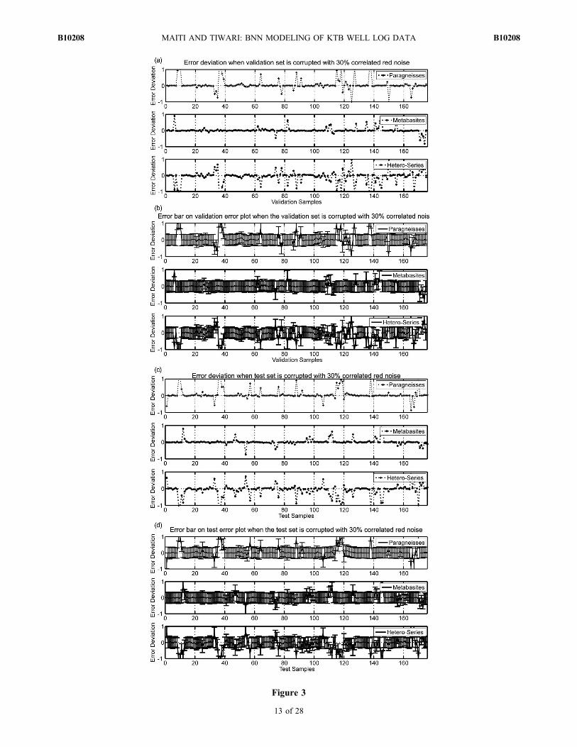
Figure 3
MAITI AND TIWARI: BNN MODELING OF KTB WELL LOG DATA B10208B10208
13 of 28

Figure 3. (continued)
MAITI AND TIWARI: BNN MODELING OF KTB WELL LOG DATA B10208B10208
14 of 28

log data. Assuming that there is some possibility of ines-capable noise in the data, it would be prudent to test therobustness and the stability of the results. For this, wegenerated correlated noise using the first‐order auto-regressive model [Fuller, 1976],
d nð Þ ¼ Ad n� 1ð Þ þ "n: ð48Þ
Here, d(n) is a stationary space series at space n and "n is aGaussian white noise with zero mean and unit variance. Theconstant A represents the maximum likelihood estimator(MLE) and can be computed from the data as [Fuller, 1976]
A nð Þ ¼P
dn�1 � dmð Þ dn � dmð Þ½ �ffiffiffiffiffiffiffiffiffiffiffiffiffiffiffiffiffiffiffiffiffiffiffiffiffiffiffiffiffiffiffiffiffiffiffiffiffiffiffiffiffiffiffiffiffiffiffiffiffiffiffiffiffiffiffiffiffiffiffiffiffiffiffiPdn�1 � dmð Þ2P dn � dmð Þ2
h ir ; ð49Þ
where d(n) is a data value at the point n, and dm is the meanvalue. Using equation (49), the MLE constant A(n) is esti-mated as 0.52 for the density data series, 0.21 for theporosity data series, and 0.53 for the gamma ray data seriesfrom the validation data sets and 0.47 for the density series,0.23 for the porosity series, and 0.55 for the gamma rayseries from the test data sets. We generated the Gaussiannoise "n using a MATLAB library function. The correlatednoisy time series (equation (48)) for each well‐log data setis, then, normalized between [−1 and +1] using
"norc nð Þ ¼ 2� "c nð Þ � "cminf Þg"cmax � "cminð Þ � 1; ð50Þ
where "cnor (n) is the normalized correlated noise and "c (n) is
the unnormalized correlated noise; "cmax and "cmin are re-presented as the maximum and the minimum value of "c (n),respectively. The normalized correlated noise for a dataseries is, then, taken to the level of the well‐log data using
d"c nð Þ ¼ d nð Þ � "norc ; ð51Þ
where d(n) is the synthetic data series (we assume synthetictraining data is noise free). Now, the correlated noise d"c (n)from equation (51) is added to the d(n) according to theequation
du nð Þ ¼ d nð Þ þ u
100
� �� d"c nð Þ: ð52Þ
Here du (n) is the data corrupted with a certain “percentage”of correlated noise in the above equation and u = 1, 2, 3,…,100. We prepared the individual data sets corrupted withdifferent level of correlated red noise. The results of stability
in presence of correlated noise are presented in Table 4. Theaccuracy of network prediction is examined using the vali-dation and the test data sets when both the data sets arecontaminated with different levels (10%–50%) of deceptivered noise. The error‐deviation plot for well‐log data cor-rupted by 30% and 50% correlated noise is presented inFigures 3a–3h. Our analyses suggest that the predictiveefficiency of the BNN is considerably robust, even if theinput well‐log data is contaminated with “red” noise up to40% or so; however, the predictive capability is degeneratedbeyond 50% noise contamination.
7. Uncertainty Analysis
[34] The uncertainty at the network output, (covariancematrix Covo = Covm + gTH−1g) is due to the intrinsic noisein the data embodied in m and the theoretical error describedby the posterior distribution of the weight vector w embod-ied in gTH−1g [Aires, 2004]. For the forward linear operator,the posterior pdf will be Gaussian, and in that case, one canassume that all uncertainties are also Gaussian. However, forthe nonlinear neural network, even if the pdf of the neuralnetwork weight is Gaussian, the pdf of the output can benon‐Gaussian [Aires, 2004]. The derivative of forwardfunction is evaluated at wMLP. Here, the mean standarddeviation (STD) ( =
ffiffiffiffiffiffiffiffiffiffiffiffiffiffiffiffiffiffiffiffiffiffidiag Covoð Þp
) is estimated by takingthe square root of the diagonal terms in Covo. The elementsalong the main diagonal of output covariance matrix showsthe “variances” of the fluctuations about the mean of theGaussian probability densities that characterizes the uncer-tainties, and the off‐diagonal elements show the extent towhich these fluctuations are correlated [Tarantola, 1987].Figure 3 shows error bars plotted on error deviation curvefor the input data which are corrupted with different level ofcorrelated deceptive noise. All error bars are ± unit standard‐deviations estimated from the a posteriori covariance matrix.Figures 4 and 5 present the mean standard deviation or threeoutputs: paragneisses, metabasites, and heterogeneousseries. The ± unit standard deviations/error bar shows the90% confidence interval (CI) [Nabney, 2004]. The mini-mum, maximum, and average values of the standard devi-ation of output error over the entire length of litho‐sectionare documented in sections 8–10.
8. Examples
[35] We used three sets of borehole data viz. density,neutron porosity, and gamma ray obtained from the German
Table 4. Showing Percentage of Accuracy While Validation and Test Data Sets are Corrupted with Different Level of Red Noise
Red Noise Level
Percentage of Accuracy in Generalization Data Set
Validation Data Set Test Data Set
Average Stability ± 5%Error LimitsParagneisses Metabasites
HeterogeneousSeries Paragneisses Metabasites
HeterogeneousSeries
0% 89.14% 85.14% 74.29% 89.20% 82.95% 72.16% 82.14%10% 86.16% 86.29% 73.14% 87.50% 82.95% 70.45% 81.08%20% 84.00% 85.71% 68.57% 84.66% 82.92% 67.31% 78.86%30% 81.14% 85.71% 66.29% 82.39% 81.82% 64.77% 77.02%40% 80.57% 85.71% 65.71% 80.68% 80.11% 61.36% 75.69%50% 78.86% 84.57% 62.86% 78.98% 79.55% 59.09% 73.98%
MAITI AND TIWARI: BNN MODELING OF KTB WELL LOG DATA B10208B10208
15 of 28

Continental Deep Drilling Program site. These data areapplied to the trained BNN network to classify the litho‐facies succession, and the BNN‐based results are comparedwith the results of the published geological section[Emmermann and Lauterjung, 1997], and our earlier resultsbased on super self adaptive back‐propagation neural net-works [Maiti et al., 2007]. Maiti et al. [2007] have devel-oped a classification scheme based on the very fast SSABPneural network theory where the learning rate is variable andadaptive to the complexity of the error surface. In thatapproach the solution obtained is based on maximum like-lihood method, where a single “best” set of weight values isevaluated by minimization of a suitable error function. TheBNN approach considers a probability distribution functionover weight space instead of a single “best” set of weights.Thus, it is quite sensible to compare the BNN results with theresults based on SSABP. The comparative results obtainedby both neural network techniques for the pilot and the mainborehole data are displayed in Figures 4 and 5, respectively.The outputs of the network represent the posterior proba-bility distribution. Further, the standard deviation errormaps, corresponding to the three types of litho‐facies arepresented to quantify the prediction uncertainties of thenetwork output over the entire KTB litho‐section. All thecomparative results shown in Figures 4 and 5 are presentedin a three‐column gray‐shaded matrix with black repre-senting 1 and white representing 0. The interpretation of themaximum a posteriori geological section (MAPGS) is asfollows: if the litho‐facies of a particular class exists, theoutput value of the node in the last layer is 1 or very close to1, and if not, it is 0 or very close to 0.
8.1. Comparisons of the BNN ResultsWith the Published Results
[36] The published results of litho‐facies successions byEmmermann and Lauterjung [1997] were re‐drawn for thesake of clarity [Maiti et al., 2007, Figure 2]. The MAPGSderived from the BNN modeling via the SCG optimizationfor both the KTB boreholes are displayed at 500 m datawindows for critical and thorough examination and com-pared with published subsections (“Subsection of KTB‐VB/HB” in Figures 4 and 5). A careful visual inspection of thesefigures suggests that the BNN results correlate fairly wellwith the published results over the entire litho‐section.
8.2. Pilot Borehole (KTB‐VB) (up to 4000 m Depth)
[37] The results based on the BNN modeling confirm, ingeneral, the presence of paragneisses, metabasites, andheterogeneous series within the first 500 m depths. How-ever, a close examination and comparison of the BNNresults with the published results reveal some dissimilaritytoo (Figure 4a). For instance, in the depth range of 30–100 m,the BNN model indicates the presence of heterogeneous
series, whilst the published subsection shows the para-gneisses unit. Likewise at the depth range of 240–250 m, theBNN results indicate the presence of paragneisses, while thepublished subsection shows the heterogeneous series. If wego further down, at the depth range of 305–340 m, the BNNresults show the presence of paragneisses, heterogeneousseries and metabasites instead of the heterogeneous seriesalone. There is also some mismatch at 400–430 m depthrange where the BNN shows the metabasites, instead of theheterogeneous series, and at the 430–490 m depth range, theBNN indicates the paragneisses instead of the heterogeneousseries.[38] There is a positive correlation between the BNN
model results and the published results (Figures 4b and 4c)at the 500–1500 m depth range which shows good confor-mity with the three litho‐facies successions (e.g., para-gneisses, metabasites and heterogeneous series). Howeverthere are some divergences too. The BNN results suggestthe presence of the paragneisses instead of the heteroge-neous series at the depth intervals 520–556 m, the hetero-geneous series instead of the paragneisses at the depthinterval of 579–582 m, the heterogeneous series instead ofthe paragneisses at the depth interval of 598–601 m, theheterogeneous series instead of the paragneisses at the depthinterval of 707–712 m, and the metabasites instead of theparagneisses at the depth interval of 1145–1168 m. Thepresent results also show good match within the depth rangeof 1500–2500 m (Figures 4d and 4e) with a few exceptions,for example, the presence of heterogeneous series at thedepth range of 1597–1618 m and the paragneisses at thedepth range of 1744–1817 m and 2442–2467 m. The BNNresults show the dominance of the paragneisses at the depthintervals of 2500–3000 m, 2562–2623 m, and 2852–2953 min addition to an inter‐bedded thin metabasites structures atthe depth range of 2640–2646 m (Figure 4f). Figure 4gexhibits the presence of the paragneisses and the heteroge-neous series that are consistent with the published resultsexcept for the depth range of 3408–3421 m. In addition tothis, the BNN results also suggest the presence of theparagneisses and the heterogeneous series at the depths in-tervals of 3204–3248 m and 3409–3418 m, respectively.Comparison of the present results at the depth range of3500–4000 m shows a depositional sequence of the para-gneisses and the metabasites that exactly match with thepublished results (Figure 4h). The minor deviations andsome differences observed between the published and thepresent result is explained in the discussion section. Theaverage standard deviation estimated at the network outputcorresponding to the paragneisses, metabasites and hetero-geneous series is ±0.30 for the entire KTB pilot hole (downto 4000 m), except for depths 58.52 m, 381.60 m, 1186.75 m,1238.09 m, and 1286.86 m, where the STD is ±0.58, ±0.78,±0.99 ±0.54 and ±0.79, respectively.
Figure 4. (a) Comparison of the maximum a posteriori geological section (MAPGS) obtained by BNN with the SCGapproach with a maximum likelihood geological section (MLGS) obtained by the SSABP neural network, and the publishedlitho‐facies subsection of pilot hole (KTB‐VB) (published litho‐subsection is redrawn after Emmermann and Lauterjung[1997]) and the standard deviation (std) error map estimated at the network output by BNN approach at the depth inter-val of 0–500 m. In this interval 0–28 m, data are not available. (b)–(h) Same for the depth range of 500–1000 m, …, 3500–4000 m in KTB pilot hole(KTB‐VB).
MAITI AND TIWARI: BNN MODELING OF KTB WELL LOG DATA B10208B10208
16 of 28

Figure 4
MAITI AND TIWARI: BNN MODELING OF KTB WELL LOG DATA B10208B10208
17 of 28

Figure 4. (continued)
MAITI AND TIWARI: BNN MODELING OF KTB WELL LOG DATA B10208B10208
18 of 28

Figure 4. (continued)
MAITI AND TIWARI: BNN MODELING OF KTB WELL LOG DATA B10208B10208
19 of 28

Figure 4. (continued)
MAITI AND TIWARI: BNN MODELING OF KTB WELL LOG DATA B10208B10208
20 of 28

8.3. Main Borehole (KTB‐HB) (up to 7000 m Depth)
[39] Comparison of the BNN modeling result of the mainKTB borehole data also exhibits, in general, good correlationwith the published results of Emmermann and Lauterjung[1997] (Figures 5a–5d). However, there are some varia-tions too. For instance, there is an evidence of bimodalcombination of the hetero‐series and the metabasitessequence at the depth interval of 4400–4500 m instead of asingle depositional sequence of the metabasites as reportedin previous investigation. Further there is also evidence forthe thinner heterogeneous series at the depths range of4580–4583 m, 4809–4812 m, and 4580–4583 m instead of asingle metabasites unit. Again at the depth interval of 5440–5500 m, there is evidence of a bimodal sequence of thehetero‐series and the metabasites instead of the metabasitesonly. Further, a closer look at Figures 5a–5d reveal thepresence of heterogeneous series, metabasites, and para-gneissess at the depth range of 5500–5650 m instead of onlymetabasites and results also suggest the presence of het-erogeneous series at the depth range of 5820–5840 minstead of the metabasites unit. It is interesting to note herethat the BNN modeling results also reveal successions of anadditional structure at the depth ranges of 6017–6026 m,6322–6334 m, and 6400–6418 m in the heterogeneousseries (Figure 5e), in addition to the main classes at thedepth interval of 5543–5560 m (Figure 5d). Figure 5f showsthe dominance of heterogeneous series. But the BNN resultsshow the presence of heterogeneous series at the depth rangeof 6550–6665 m instead of the metabasites and the hetero-geneous series and results also indicate the presence ofheterogeneous series and the metabasites at the depthinterval of 6710–7000 m instead of a single metabasites unit.The average standard deviation estimated at the networkoutput corresponding to the paragneisses, metabasites, andheterogeneous series is ±0.30 for the entire KTB main hole(here, 4000–7000 m), except for depths 4624.73 m,5647.33–5650.38 m, and 5682.38 m, where the standarddeviation is ±0.44, ±0.68, and ±0.87, respectively.
9. Computation Time
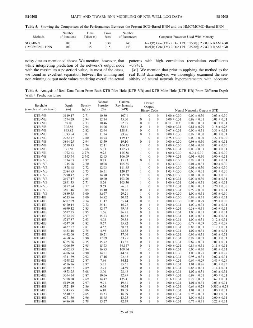
[40] Table 5 compares performances in terms of the exe-cution(CPU) time, error bars, number of iterations, numberof parameters, and processor/memory used between thecurrent SCG‐based BNN method and the hybrid MonteCarlo (HMC)/Markov Chain Monte Carlo (MCMC)‐basedBNN method [Maiti and Tiwari, 2009, 2010]. We selected afixed number (100) of iterations instead of an arbitrarystopping criterion. For the comparison, the simulations weredone with MLP network with 20 hidden nodes. The initialprior hyperparameters and the number of training examples(351) were also kept unchanged for both the simulation.Table 5 shows that the SCG‐based BNN requires less exe-cution time at the cost of error bars compared to the HMC/
MCMC‐based BNN. Experimental results show that usinglarge amounts of training data the SCG‐based BNN andHMC/MCMC‐based BNN performance are similar, but theMCMC method seems superior on smaller‐sized trainingsets. We note that the disadvantage of the present SCG‐based BNN method for small data sets, namely that a largepart of the computational effort is taken up with the inver-sion of the Hessian. Thus, the Bayesian approach is unde-niably expensive in computational load, but in complexreal‐world problems there are few cheap alternatives.
10. Discussions
[41] Comparison of the MAPGS with the published litho‐species section of Emmermann and Lauterjung [1997]exhibits more or less matching patterns (Figures 4 and 5).In addition to this, the BNN model reveals some finerstructural details, which might be geologically significant.We note, however, that in such complex geological situa-tions, it is somewhat intricate to assert an exact geologicalinterpretation for these thin successions as to whether theseapparently visible finer details inferred from our study aretruly meaningful geological structures or simply an artifactof our analysis. To examine the authenticity of these struc-tural details, we manually checked a few samples producedby the trained network with the limited core knowledgedefined in Table 2 (comparison is given in Table 6). It isinteresting to see that the trained network produces more orless identical results that are consistent with the trainingdata. We note, however, that the present probabilistic his-togram model of litho‐facies classification cannot beuniquely constrained and/or compared with the existinglitho‐section [Maiti et al., 2007, Figure 2]. The reason beingthat the published results are mostly gross‐average depthsections estimated from the litho‐sections. The second rea-son could be that the observed data may be biased withsome deceptive “red noise” signals with nonzero mean.Hence, it is likely that there could be some possibility oferror due to lack of resolution in the KTB data. It is note-worthy, however, that most of the deviations and differencesbetween the published and the BNN model were observed inthe pilot borehole and moreover in the upper part of thecrust.[42] Further we note that there are some mismatches
between the present model and the published model. Thestandard deviation error map, which shows uncertainty inthe classification of the litho‐facies boundaries, is preparedbased on the clear distinction between the winner and thenon‐winner node values. A standard deviations with a largerthan average value shows more uncertainty in prediction andvice versa. In some cases, however, we found that thestandard deviation values are more even when the maximuma posteriori probability is comparable to the litho‐faciesunits. This seems to have occurred in the estimation ofuncertainty in terms of probability distribution functions of
Figure 5. (a) Comparison of a maximum a posteriori geological section (MAPGS) obtained by BNN with the SCGapproach with the maximum likelihood geological section (MLGS) obtained by the SSABP neural network approach withthe published litho‐facies subsection of main hole (KTB‐HB) (published litho‐subsection is redrawn after Emmermann andLauterjung [1997]) and the standard deviation (std) error map estimated at the network output by the BNN approach at thedepth interval of 4000–4500 m. (b)–(f) Same for the depth range of 4500–5000 m, …, 6500–7000 m in KTB main hole(KTB‐HB).
MAITI AND TIWARI: BNN MODELING OF KTB WELL LOG DATA B10208B10208
21 of 28

Figure 5
MAITI AND TIWARI: BNN MODELING OF KTB WELL LOG DATA B10208B10208
22 of 28
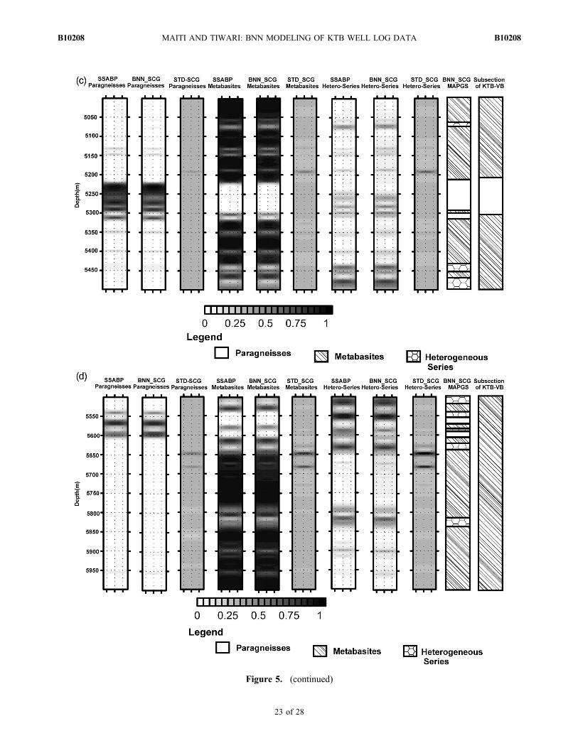
Figure 5. (continued)
MAITI AND TIWARI: BNN MODELING OF KTB WELL LOG DATA B10208B10208
23 of 28

Figure 5. (continued)
MAITI AND TIWARI: BNN MODELING OF KTB WELL LOG DATA B10208B10208
24 of 28
noisy data as mentioned above. We mention, however, thatwhile interpreting prediction of the network’s output nodewith the maximum a posteriori value, in most of the cases,we found an excellent separation between the winning andnon‐winning output node values rendering overall the actual
patterns with high correlation (correlation coefficients∼0.943).[43] We mention that prior to applying the method to the
real KTB data analysis, we thoroughly examined the sen-sitivity of neural network hyperparameters with adequate
Table 6. Analysis of Real Data Taken From Both KTB Pilot Hole (KTB‐VB) and KTB Main Hole (KTB‐HB) From Different DepthWith ± Prediction Error
Borehole(samples of data taken)
Depth(m)
Density(g/cc)
NeutronPorosity(%)
GammaRay Intensity
(API)
DesiredOutput/
Binary Code Neural Networks Output ± STD
KTB‐VB 3119.17 2.71 10.80 107.1 1 0 0 1.00 ± 0.30 0.00 ± 0.30 0.03 ± 0.30KTB‐VB 1574.29 2.94 12.34 45.00 0 1 0 0.00 ± 0.31 0.98 ± 0.31 0.01 ± 0.31KTB‐VB 89.00 2.73 10.46 82.05 0 0 1 0.05 ± .0.31 0.02 ± 0.31 0.83 ± 0.31KTB‐VB 305.86 2.94 14.06 32.61 0 1 0 0.00 ± 0.31 0.81 ± 0.29 0.18 ± 0.28KTB‐VB 893.82 2.82 12.94 128.41 0 0 1 0.67 ± 0.31 0.00 ± 0.31 0.31 ± 0.31KTB‐VB 1393.54 3.01 11.24 23.26 0 1 0 0.00 ± 0.30 0.99 ± 0.30 0.01 ± 0.31KTB‐VB 2252.47 2.80 14.94 119.17 1 0 0 0.75 ± 0.30 0.00 ± 0.30 0.22 ± 0.30KTB‐VB 3864.25 2.94 13.59 19.10 0 1 0 0.00 ± 0.30 0.98 ± 0.30 0.01 ± 0.31KTB‐VB 3559.45 2.74 12.11 104.35 1 0 0 1.00 ± 0.30 0.01 ± 0.30 0.03 ± 0.30KTB‐VB 771.60 2.68 5.33 112.73 1 0 0 0.96 ± 0.31 0.00 ± 0.31 0.01 ± 0.31KTB‐VB 1072.43 2.776 9.72 115.58 1 0 0 1.00 ± 0.30 0.0 ± 0.30 0.02 ± 0.30KTB‐VB 1145.74 2.745 12.03 106.69 1 0 0 0.99 ± 0.31 0.01 ± 0.30 0.00 ± 0.31KTB‐ VB 1374.03 2.97 8.73 15.83 0 1 0 0.00 ± 0.30 0.99 ± 0.31 0.01 ± 0.31KTB‐ VB 1715.26 2.70 10.08 105.55 1 0 0 1.02 ± 0.30 0.01 ± 0.31 0.00 ± 0.30KTB‐ VB 1878.48 2.72 12.03 111.65 1 0 0 1.00 ± 0.30 0.01 ± 0.30 0.00 ± 0.30KTB‐ VB 2084.83 2.75 16.51 120.17 1 0 0 1.03 ± 0.30 0.00 ± 0.31 0.01 ± 0.30KTB‐ VB 2290.42 2.75 14.70 119.58 1 0 0 0.96 ± 0.30 0.01 ± 0.30 0.02 ± 0.30KTB‐ VB 2697.17 2.65 10.00 103.20 1 0 0 1.02 ± 0.31 0.00 ± 0.30 0.01 ± 0.31KTB‐ VB 2891.33 2.71 8.76 103.30 1 0 0 1.00 ± 0.31 0.01 ± 0.31 0.02 ± 0.31KTB‐ VB 3177.84 2.77 9.69 96.31 1 0 0 0.78 ± 0.31 0.02 ± 0.31 0.20 ± 0.30KTB‐ VB 3801.16 3.04 14.10 30.46 0 1 0 0.00 ± 0.31 0.99 ± 0.30 0.01 ± 0.31KTB‐ VB 3889.55 3.00 8.677 29.21 1 0 0 0.00 ± 0.30 1.00 ± 0.31 0.03 ± 0.30KTB‐HB 6515.86 3.00 14.82 20.32 0 1 0 0.00 ± 0.30 0.99 ± 0.31 0.00 ± 0.31KTB‐HB 6807.09 2.74 11.17 55.44 0 0 1 0.00 ± 0.30 0.05 ± 0.29 0.95 ± 0.30KTB‐HB 6470.14 2.72 25.11 16.72 0 1 0 0.00 ± 0.31 1.00 ± 0.31 0.01 ± 0.31KTB‐HB 6999.12 2.85 12.47 49.45 0 0 1 0.00 ± 0.31 0.38 ± 0.31 0.61 ± 0.31KTB‐HB 5677.35 2.95 1.66 26.75 0 1 0 0.00 ± 0.31 1.00 ± 0.31 0.03 ± 0.31KTB‐HB 5372.25 2.97 15.23 16.83 0 1 0 0.00 ± 0.31 1.00 ± 0.31 0.02 ± 0.31KTB‐HB 5217.87 2.93 4.08 29.53 0 1 0 0.00 ± 0.31 1.00 ± 0.31 0.12 ± 0.31KTB‐HB 4547.00 2.82 8.67 35.92 0 1 0 0.00 ± 0.30 0.79 ± 0.29 0.22 ± 0.29KTB‐HB 4427.37 2.81 4.52 38.63 0 1 0 0.00 ± 0.31 0.88 ± 0.31 0.17 ± 0.31KTB‐HB 4433.16 2.75 4.89 42.33 0 1 0 0.00 ± 0.31 1.02 ± 0.31 0.01 ± 0.31KTB‐HB 4442.00 2.92 10.21 37.06 0 1 0 0.00 ± 0.31 0.99 ± 0.31 0.01 ± 0.31KTB‐HB 4950.56 2.90 12.09 33.75 0 1 0 0.01 ± 0.31 0.99 ± 0.31 0.03 ± 0.31KTB‐HB 6325.36 2.75 15.72 13.35 0 1 0 0.01 ± 0.31 0.87 ± 0.31 0.01 ± 0.31KTB‐HB 4006.59 2.95 15.73 36.147 0 1 0 0.00 ± 0.31 0.84 ± 0.31 0.15 ± 0.31KTB‐HB 4002.93 2.84 16.83 109.94 1 0 0 1.00 ± 0.31 0.00 ± 0.30 0.01 ± 0.31KTB‐HB 4206.24 2.90 14.51 44.58 0 1 0 0.00 ± 0.30 1.00 ± 0.27 0.05 ± 0.27KTB‐HB 4311.39 2.92 17.16 22.42 0 1 0 0.00 ± 0.31 0.98 ± 0.31 0.02 ± 0.31KTB‐HB 4548.22 2.87 7.96 34.12 0 1 0 0.00 ± 0.31 0.64 ± 0.29 0.41 ± 0.29KTB‐HB 4556.76 2.97 5.31 25.51 0 1 0 0.00 ± 0.31 1.01 ± 0.26 0.03 ± 0.25KTB‐HB 4630.67 2.89 2.73 24.59 0 1 0 0.01 ± 0.31 0.85 ± 0.31 0.14 ± 0.31KTB‐HB 4873.75 3.08 3.00 28.48 0 1 0 0.00 ± 0.31 1.02 ± 0.31 0.01 ± 0.31KTB‐HB 5054.34 2.87 10.66 32.95 0 1 0 0.00 ± 0.31 0.99 ± 0.31 0.00 ± 0.31KTB‐HB 5058.30 2.69 14.47 135.41 0 0 1 0.16 ± 0.31 0.22 ± 0.31 0.62 ± 0.31KTB‐HB 5149.90 2.97 9.91 19.61 0 1 0 0.00 ± 0.31 1.01 ± 0.31 0.03 ± 0.31KTB‐HB 5321.19 2.86 6.56 40.54 0 1 0 0.03 ± 0.31 0.64 ± 0.28 0.380 ± 0.28KTB‐HB 5743.95 3.06 6.10 18.39 0 1 0 0.00 ± 0.31 1.01 ± 0.31 0.00 ± 0.31KTB‐HB 5840.27 2.65 14.53 16.09 0 1 0 0.00 ± 0.31 0.98 ± 0.31 0.00 ± 0.31KTB‐HB 6271.56 2.96 18.45 13.75 0 1 0 0.00 ± 0.31 1.00 ± 0.31 0.00 ± 0.31KTB‐HB 6486.90 2.78 15.27 42.39 0 1 0 0.00 ± 0.31 0.77 ± 0.31 0.22 ± 0.31
Table 5. Showing the Comparison of the Performances Between the Present SCG‐Based BNN and the HMC/MCMC‐Based BNN
MethodsNumber
of IterationsTime
Taken (s)ErrorBars
Numberof Parameters Computer Processor Used With Memory
SCG‐BNN 100 3 0.30 143 Intel(R) Core(TM) 2 Due CPU E7500@ 2.93GHz RAM 4GBHMC/MCMC‐BNN 100 15 0.15 143 Intel(R) Core(TM) 2 Due CPU E7500@ 2.93GHz RAM 4GB
MAITI AND TIWARI: BNN MODELING OF KTB WELL LOG DATA B10208B10208
25 of 28

empirical examples for network prediction. The experimentguided us to choose appropriate hyperparameters for theactual data analysis. In this way, we could also fairly ruleout the uncertainty due to choosing the appropriate hy-perparameters in interpretation. The experimental dataanalysis suggests that the true prediction heavily depends on
the ratio�
�. Accordingly, the hyperparameter was set in for
the real KTB data analysis. Further regression analysis ofboth borehole results and between two approaches (SSABPand BNN–SCG) also shows consistent and good agreements(R ∼ 0.97) (Figures 6a–6f).[44] It may thus be emphasized that the BNN algorithm
employed here combined with its validation, test and
regression analyses do provide credentials to the presentresults. As discussed above, despite various sources oferrors, the apparently visible changes in litho‐logs succes-sions appears to be the inter‐bedded geological structuresthat remained ambiguous/unrecognized in earlier qualitativeinvestigations. The output of the histogram type networksfor choosing a maximum a posterior probability value, asdiscussed in detail by Bishop [1995], is more appropriateand provides better guidance on data analysis for such acomplex data analysis.
11. Conclusions
[45] A new BNN approach [Nabney, 2004] is employed todecode changes in layer successions from well‐log data. The
Figure 6. (a–f) Regression analysis of pilot hole (KTB‐VB) and KTB main hole (KTB‐HB) correspondsto the paragneisses, metabasites, and hetero‐series shows very good agreement between the BNN and theSSABP results. A dashed line indicates the best linear fit (slope 1 and y‐intercept 1). The solid line in thefigure shows the perfect fit. The correlation coefficient (R), between the two approaches actually, mea-sures how well the variation is in two results. If this number is equal to 1, there is a perfect correlationbetween the two approaches.
MAITI AND TIWARI: BNN MODELING OF KTB WELL LOG DATA B10208B10208
26 of 28

stability and the efficiency of the BNN approach areexamined on empirically generated noisy as well as noise‐free data sets. The BNN has inherent ability to approximatethe functional relationship between the input and the outputspace/domain by learning through examples, even if there isno deterministic relationship between the input and theoutput space/domain. The method provides a neat andtractable mathematical framework in which the networkweights could be adjusted in a fully probabilistic way. Theproposed method is robust for uncertainty analysis and takescare of over‐fitting and under‐fitting in a natural way. TheBNN technique is also an efficient and cost‐effective tool tointerpret a large amount of borehole log data. This providesa good testimony to use the BNN‐based techniques to solvethe nonlinear inversion problem for borehole geophysics.[46] The BNN approach is then successfully applied to
classify changes in the litho‐facies boundaries from the realwell‐log data obtained from the German Continental DeepDrilling site. The method essentially allows us to estimateuncertainty in network prediction along the entire length oflitho‐section of the KTB. Some mismatching observed inthe BNN analysis might result due to the presence of redsignals with nonzero mean and/or lack of resolution in theKTB data. Over all the results of present analyses suggestthat, besides corroborating well with the existing results onthe KTB site, the method also uncovers additional finerdetails of intervening layer successions in the bigger geo-logical units, which seem to be of some geological signifi-cance and should form the basis for more detailedquantitative examination. Thus, besides introducing a newprobabilistic inversion scheme to the problems of well‐logdata for litho‐facies classification, the present analysis alsoreveals some new results and thus explores the generality ofthe new method for its actual application to other domains ofearth sciences. Because of its computational efficiency, it isproposed that the BNN methods could be further exploitedfor analyzing a large amount of borehole data in some othergeologically complex areas of interest.
[47] Acknowledgments. We would like to thank Ian T. Nabney forproviding the Netlab tool box from which some of the routines have beenused in the work. Saumen Maiti expresses sincere thanks to Department ofScience and Technology, Government of India to carry out the researchwork. We are also grateful to the Director of the National GeophysicalResearch Institute (CSIR) and the Director of the Indian Institute of Geo-magnetism, Navi‐Mumbai, for their kind permission to publish this work.We are also thankful to Prof. Hans‐Joachim Kumpel for providing the KTBdata.
ReferencesAires, F. (2004), Neural network uncertainty assessment using Bayesianstatistics with application to remote sensing: 1. Network weights,J. Geophys. Res., 109, D10303, doi:10.1029/2003JD004173.
Aristodemou, E., C. Pain, C. Oliveira, and T. Goddard (2005), Inversion ofnuclear well‐logging data using neural networks, Geophys. Prospect., 53,103–120.
Baldwin, J., A. R. M. Bateman, and C. L. Wheatley (1990), Application ofneural network to the problem of mineral identification from well logs,Log Anal., 31, 279–293.
Benaouda, D., G.Wadge, R. B.Whitmarsh, R. G. Rothwell, and C.MacLeod(1999), Inferring the lithology of borehole rocks by applying neuralnetwork classifiers to downwhole logs: An example from the OceanDrilling Program, Geophys. J. Int., 136, 477–491.
Berckhemer, H., A. Rauen, H. Winter, H. Kern, A. Kontny, M. Lienert,G. Nover, J. Pohl, T. Popp, A. Schult, J. Zinke, and H. C. Soffel (1997),
Petrophysical properties of the 9‐km deep crustal section at KTB,J. Geophys. Res., 102(B8), 18337–18361.
Bescoby, D. J., G. C. Cawley, and P. N. Chroston (2006), Enhanced inter-pretation of magnetic survey data from archaeological sites using artifi-cial neural networks, Geophysics, 71(5), H45–H53.
Bishop, C. M. (1995), Neural Networks for Pattern Recognition, OxfordUniversity Press, Oxford.
Bosch, M. (1999), Lithologic tomography: From plural geophysical data tolithology estimation, J. Geophys. Res., 104(B1), 749–766.
Bosch, M., and J. McGaughey (2001), Joint inversion of gravity and mag-netic data under lithologic constraints, Leading Edge, 20, 877–881.
Bosch, M., A. Gullen, and P. Ledru (2001), Lithologic tomography: Anapplication to geophysical data from the Cadomian belt of northernBrittany, France, Tecton., 331, 197–227.
Buntine, W. L., and A. S. Weigend (1991), Bayesian back propagation,Complex Syst., 5, 603–643.
Busch, J. M., W. G. Fortney, and L. N. Berry (1987), Determination oflithology from well logs by statistical analysis, SPE Form. Eval., 2,412–418.
Calderon‐Macias, C., M. K. Sen, and P. L. Stoffa (2000), Artificial neuralnetworks for parameter estimation in geophysics, Geophys. Prosp., 48,21–47.
Coppola, E. A., Jr., A. J. Rana, M. M. Poulton, F. Szidarovszky, and V. W.Uhl (2005), A neural network model for predicting aquifer water levelelevations, Ground Water, 43(2), 231–241.
Coulibaly, P., F. Anctil, and B. Bobee (2001), Multivariate reservoir inflowforecasting using temporal neural networks, J. Hydrol. Eng., 6, 367–376.
Dai, H., and C. Macbeth (1995), Automatic picking of seismic arrivals inlocal earthquake data using an artificial neural network, Geophys. J. Int.,120, 758–774.
Delfiner, P., O. Peyret, and O. Serra (1987), Automatic determination oflithology from well logs, SPE Form. Eval., 2, 303–310.
Devilee, R. J. R., A. Curtis, and K. Roy‐Chowdhury (1999), An efficientprobabilistic neural network approach to solving inverse problems:Inverting surface wave velocities for Eurasian crustal thickness, J. Geophys.Res., 104(12), 28,841–28,856.
Dystart, P. S., and J. J. Pulli (1990), Regional seismic event classification atthe NORESS array: Seismological measurements and use of trainedneural network, Bull. Seis. Soc. Am., 80, 1910–1933.
Emmermann, R., and J. Lauterjung (1997), The German Continental DeepDrilling Program KTB: Overview and major results, J. Geophys. Res.,102, 18179–18201.
Feng, X.‐T., M. Seto, and K. Katsuyama (1997), Neural dynamic modelingon earthquake magnitude series, Geophys. J. Int., 128, 547–556.
Franke, W. (1989), The geological framework of the KTB drill site, inThe German Continental Deep Drilling Program (KTB), edited byR. Emmermann and J. Wohlenberg, pp. 38–54, Springer, Berlin.
Fuller, W. A. (1976), Introduction to Statistical Time Series, John Wiley,New York.
Gassaway, G. R., D. R. Miller, L. E. Bennett, R. A. Brown, M. Rapp, andV. Nelson (1989), Amplitude variations with offset: Fundamentals andcase histories, SEG Continuing Education Course Notes.
Helle, H. B., A. Bhatt, and B. Ursin (2001), Porosity and permeability pre-diction from wireline logs using artificial neural networks: A North Seacase study, Geophys. Prosp., 49, 431–444.
Khan, M. S., and P. Coulibaly (2006), Bayesian neural network for rainfall‐runoff modeling, Water Resour. Res., 42, W07409, doi:10.1029/2005WR003971.
Leonardi, S., and H. Kumpel (1998), Variability of geophysical log dataand signature of crustal heterogeneities at the KTB, Geophys. J. Int.,135, 964–974.
Leonardi, S., and H. Kumpel (1999), Fractal variability in super deepborehole‐implications for the signature of crustal heterogeneities, Tecto-nophysics, 301, 173–181.
MacKay, D. J. C. (1992), A practical Bayesian framework for back‐propagation networks, Neural Comput., 4(3), 448–472.
Maiti, S., and R. K. Tiwari (2009), A hybrid Monte Carlo method basedartificial neural networks approach for rock boundaries identification:A case study from the KTB bore hole, Pure Appl. Geophys., 166,2059–2090, doi:10.1007/s00024-009-0533-y.
Maiti, S., and R. K. Tiwari (2010), Automatic discriminations of geophysicalsignals using the Bayesian neural networks approach, Geophysics, 75(1),E67–E78, doi:10.1190/1.3298501.
Maiti, S., R. K. Tiwari, and H. J. Kumpel (2007), Neural network modelingand classification of lithofacies using well log data: A case study fromKTB borehole site, Geophys. J. Int., 169, 733–746.
McCormack, M. D., D. Zaucha, and D. Dushek (1993), First break refrac-tion event picking and seismic data trace editing using neural networks,Geophysics, 58, 67–78.
MAITI AND TIWARI: BNN MODELING OF KTB WELL LOG DATA B10208B10208
27 of 28

Meier, U., A. Curtis, and J. Trampert (2007), Global crustal thickness fromneural network inversion of surface wave data, Geophys. J. Int., 169,706–722.
Moller, M. (1993), A scaled conjugate gradient algorithm for fast super-vised learning, Neural Networks, 6, 525–533.
Mosegaard, K., and A. Tarantola (1995), Monte Carlo sampling of solu-tions to inverse problem, J. Geophys. Res., 100(B7), 12,431–12,447.
Murat, M. E., and A. J. Rudman (1992), Automated first arrival picking: Aneural network approach, Geophys. Prosp., 40, 587–604.
Nabney, I. T. (2004), Netlab Algorithms for Pattern Recognition, Springer,New York.
Neal, R. M. (1993), Bayesian learning via stochastic dynamics, in Advancesin Neural Information Processing Systems, vol. 5, edited by C. L. Gileset al., pp. 475–482, Morgan Kaufmann, San Francisco, Calif.
Pechnig, P., S. Haverkamp, J. Wohlenberg, G. Zimmermann, andH. Burkhardt (1997), Integrated interpretation in the German ContinentalDeep Drilling Program: Lithology, porosity, and fracture zones, J. Geo-phys. Res., 102, 18,363–18,390.
Pickett, G. R. (1963), Acoustic character logs and their application in for-mation evaluation, J. Petr. Tech., 15, 659–667.
Poulton, M., (Ed.) (2001), Computational Neural Networks for GeophysicalData Processing, Pergamon, Oxford, U.K.
Raiche, A. (1991), A pattern recognition approach to geophysical inversionusing neural nets, Geophys. J. Int., 105, 629–648.
Rogers, S. J., J. H. Fang, C. L. Karr, and D. A. Stanley (1992), Determinationof lithology from well logs using a neural network, AAPG Bull., 76(5),731–739.
Rosenblatt, F. (1958), The perceptron: A probabilistic model for informa-tion storage and organization in the brain, Psychol. Rev., 65, 386–408.
Roth, G., and A. Tarantola (1994), Neural networks and inversion ofseismic data, J. Geophys. Res., 99, 6753–6768.
Rumelhart, D. E., G. E. Hinton, and R. J. Williams (1986), Learning repre-sentations by back‐propagating errors, Nature, 323, 533–536.
Sambridge, M., and K. Mosegaard (2002), Monte Carlo methods in geo-physical inverse problems, Rev. Geophys., 40(3), 1009, doi:10.1029/2000RG000089.
Sen, M. K., and P. Stoffa (1996), Bayesian inference, Gibbs’ sampler anduncertainty estimation in geophysical inversion, Geophys. Prospect., 44,313–350.
Spichak, V., and I. Popova (2000), Artificial neural network inversion ofMagnetotelluric data in terms of three‐dimensional earth macropara-meters, Geophys. J. Int., 142, 15–26.
Tarantola, A. (1987), Inverse Problem Theory, Elsevier, New York.Tarantola, A. (2006), Popper, Bayes and the inverse problem, Nat. Phys.,492–494.
Van der Baan, M., and C. Jutten (2000), Neural networks in geophysicalapplications, Geophysics, 65, 1032–1047.
Walker, A. M. (1969), On the asymptotic behaviour of posterior distribu-tions, J. R. Stat., 31, 80–88.
Williams, P. M. (1995), Bayesian regularization and pruning using aLaplace prior, Neural Comput., 7, 117–143.
Wolff, M., and J. Pelissier‐Combescure (1982), FACIOLOG: Automaticelectrofacies determination: SPWLA Annual Logging Symposium paperFF, 6–9.
S. Maiti, Indian Institute of Geomagnetism, Navi‐Mumbai‐410218,India. ([email protected])R. K. Tiwari, National Geophysical Institute (CSIR), Hyderabad‐500007,
India.
MAITI AND TIWARI: BNN MODELING OF KTB WELL LOG DATA B10208B10208
28 of 28