neural flight control autopilot system
TRANSCRIPT
NNEEUURRAALL FFLLIIGGHHTT CCOONNTTRROOLL AAUUTTOOPPIILLOOTT SSYYSSTTEEMM
Qiuxia Liang Technical / Report DKS-04-04/ICE 09 July, 2004 Mediamatics / Data and Knowledge Systems group

Q.Liang ([email protected]) “Neural Flight Control Autopilot System” Technical / Report DKS-04-04/ICE 09 July, 2004 Mediamatics / Data and Knowledge Systems group Faculty of Electrical Engineering, Mathematics and Computer Science Delft University of Technology, The Netherlands http://www.kbs.twi.tudelft.nl

i
Abstract Nowadays as the need for automatic vehicle control grows, more and more researches have been done in this field, and different approaches have been adopted to design a controller system. The aim of this project is to design and implement a neural flight control system handling the basic flight behaviors of an airplane in a computer simulation environment. The whole system is divided into 3 modules, the Graphic User Interface module, the Flight Planning Module and the Neural Controller Module. The GUI module will accept the flight order from the user. The Neural Controller Module is used to provide the adaptive flight control. The Flight Planning Module is working in the higher level to manage the global control in this autopilot system. The results demonstrate that this neural flight control system is able to control the airplane, Cessna 172, to take off, fly up and to fly down, and the airplane under control is flying stably.
ii
Preface This is my final project report for the degree of Master of Science. I am doing the final project at the Knowledge Based Systems group of the faculty of Electrical Engineering, Mathematics and Computer Science at the Delft University of Technology. This goal of my project is to build a neural flight control system and investigate the ability of the neural network used in the flight control. This report is divided into 3 parts, the system design part, the system implementation part, and the conclusions part. The report starts with an introduction that explains this project and its goals. In the following chapter 2, with a brief background introduction to the airplane, I give an airplane system model used for this application. Chapter 3 talks about the neural network controller, including its background, its principle and its topologies. I explain 3 mostly used neural network controller topologies in detail and make a comparison between them, which finally results in the topology suitable for my application. Chapter 4 and chapter 5 explain the structures of the neural flight controller system, how each module has been divided and the functions for each module. Chapter 6, 7, 8 present the implementation process for the 3 system modules. Finally you may find the system testing result and the conclusions in chapter 9 and chapter 10. Acknowledgement I would like to thank dr. drs. L.J.M. Rothkrantz and ir. P.A.M. Ehlert, who give me many helpful advises and information during the project. Also thanks should be given to those people working on the SNNS project. Their powerful and open source neural network simulator takes many extra troubles from me. Finally I want to give my special thanks to my parents and all my friends.

Contents
iii
Contents 1 Introduction ………………………………………………………………………….1
1.1 Crew Assistance System – Intelligence Cockpit Environment ……………….1 1.2 The Neural Flight Control System ……………………………………………..1 1.3 Project Goal ……………………………………………………………………...3
Part I System Design 2 Flying Analysis ………………………………………………………………………7
2.1 Aviation Introduction……………………………………………………………..7 2.2 Flying Process Analysis…………………………………………………………..8 2.3 The Aviation Parameters in Modeling ………………………………………….10
3 Neural Network in Adaptive Control …………………………………………….13
3.1 Introduction ……………………………………………………………………13 3.2 The Non-hybrid and Desired Output Signal Control Strategy …………..…15
3.2.1 Direct Inverse Control …………………………………………..……….15 3.2.2 Forward Modeling and Inverse Control ………………………...……….16 3.2.3 Neural Predictive Control ……………………………………….………17 3.2.4 Comparisons …………………………………………………………….18
3.3 Identifier ……...………………………………………………………………...20 3.3.1 The Memory PE …………………………………………………………20 3.3.2 TDNN Applications ……………………………………………………..22 3.3.3 Partial Recurrent Neural Network ………………………………………23
4 SystemDesign ……………………………………………………….……………25
4.1 General System Scheme……………………………………………………..25 4.2 The Graphic User Interface Module ……………………………………….26 4.3 The Flight Planning Module………………………………………………...27 4.4 The Neural Network Controller Module ………………….……………….30
5 Module Specifications ……………………………………………………………...33
5.1 Modules and Module Specifications …………………………………………..33 5.2 The Interaction Relationship ………………………………………………….33 5.3 The Server-Client Structure …………………………………………………..35
Contents
iv
Part II System Implementation 6 Neural Controller Module Implementation ……………………………….……...…39
6.1 Process Analysis and Flow Chart …………………………………………...…..39 6.2 Stuttgart Neural Network Simulator ……………………………………….……41 6.3 Identifier Modeling ………………………………………………………..…….41
6.3.1 NARMA vs. Jordan Network …………………………………………...41 6.3.2 Identifiers’ Constructing ….…………………..…………………………42 6.3.3 Data Scaling …………. …………………………………………………45 6.3.4 The Training Set and the Pattern File …………………………………...45 6.3.5 The Identifiers’ Training ………………………………………………...47 6.3.6 Comparison ……………………………………………………………...48
6.4 The Forward Modeling and Inverse Controller ………………………….……..49 6.5 Module Test …………………………………………………………………….49
7 Flight Plan Module Implementation …………………………………………...…53
7.1 Process Analysis and Flow Chart …………………………………………….53 7.2 Module’s Programming and Testing ………………………………………...55
8 Graphic User Interface Module Implementation ………………………………..57
8.1 Implementation …………………………………………………………….…..57 8.2 Module Testing …………………………………………………………….…...58
Part III Results, Conclusions and Recommendations 9 System Testing and Improvements ……………………………………………….63
9.1 Using this Neural Flight Controller Program ………………………………..63 9.1.1 Setting a Flight Order and Start Flying ………………………………….63 9.1.2 Change the Flight Goal ………………………………………………….64 9.1.3 Stop once Flight Controlling …………………………………………….65 9.1.4 Visualizing the Flying Data ……………………………………………..65 9.1.5 Quit ………...……………………………………………………………65
9.2 System Testing …………………………………………………………………66 9.2.1 Testing the Control Function ……………………………………………66 9.2.2 Testing the Visualization Function ……………………………………...68 9.2.3 Estimating the Identifier Output ………………………………………...71 9.2.4 Testing the Miscellaneous Function …………………………………….72
9.3 Improvements ………………………………………………………………….72 9.4 Controller Stability Analysis ………………………………………………….76
10 Conclusions and Discussions ………………………………………………………79
10.1 Conclusions ……………………………………………………………………79 10.2 Discussions and Future Work ………………………………………………..81

Contents
v
Appendix
A. Aviation Introduction ………………………………………….…………………..85
A.1 Flight Controls – Ailerons, Elevator, and Rudder …………………………..85 A.2 Primary Instruments ………………………………………………………….88
B. Stuttgart Neural Network Simulator ………………………………………….….90
C. FSUIPC Module …………………………………………………………………….93
D. Neural Controller Module Implementation Details ………………………………94 References

6
Chapter 1 Introduction
1
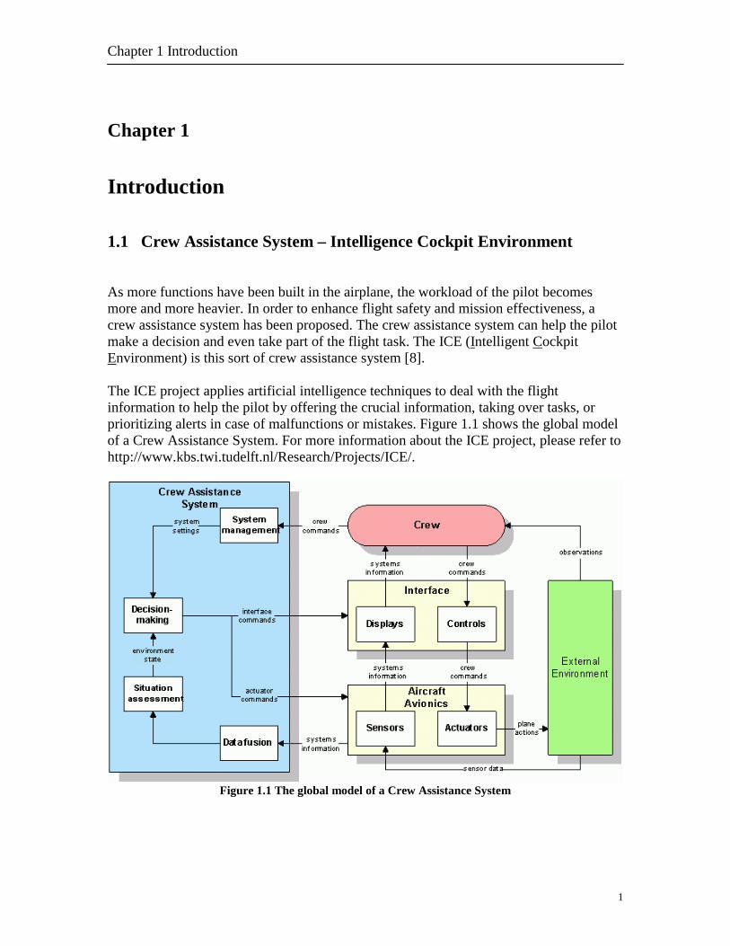
Chapter 1 Introduction 1.1 Crew Assistance System – Intelligence Cockpit Environment As more functions have been built in the airplane, the workload of the pilot becomes more and more heavier. In order to enhance flight safety and mission effectiveness, a crew assistance system has been proposed. The crew assistance system can help the pilot make a decision and even take part of the flight task. The ICE (Intelligent Cockpit Environment) is this sort of crew assistance system [8]. The ICE project applies artificial intelligence techniques to deal with the flight information to help the pilot by offering the crucial information, taking over tasks, or prioritizing alerts in case of malfunctions or mistakes. Figure 1.1 shows the global model of a Crew Assistance System. For more information about the ICE project, please refer to http://www.kbs.twi.tudelft.nl/Research/Projects/ICE/.
Figure 1.1 The global model of a Crew Assistance System
Neural Flight Control Autopilot System
2
1.2 The Neural Flight Control System While the Intelligent Cockpit Environment is designed to help the pilot to make decisions and to take part of flight task, the Neural Flight Control Autopilot system is developed as part of the ICE project, the objective of which is to control some basic flight tasks. In order to provide the consistent controlling qualities the neural network based approach has been selected for the controller module, instead of the expert system or the conventional controller. Choosing this could avoid indicating the explicit flight rules or avoid looking for the extensive gainscheduling parameters, because the flight rules and the parameters may differ in airplanes and flight environment. There are many neural controller structures available. The control structure I used for this application is called the Feed Forward and Inverse Control, which is build by two neural networks. One is a pre-trained network and another is an online learning network for inverse control. The reasons I choose this structure and the characteristics of this structure are explained in chapter 3. Once built, the neural flight control system could be applied to different aircraft applications. The architecture will remain the same. The required work is only to replace the pre-trained neural network (identifier) to another suitable one and to indicate the desired output of the airplane for each flight procedure. In this application the evaluation is performed in the Microsoft Flight Simulator 2002, and the airplane used to control is the Cessna 172. 1.3 The Project Goal The general goal for this project is to develop a neural flight control system handling the basic flight behaviors of an airplane, which are taking off, flying up, and flying down, in a computer simulation environment. The general goal can be elaborated as the following: - Design a flight control system adopting the neural network control technique; - Develop a prototype running in a computer simulated environment; - Investigate the ability of this neural flight control system. The requirements for this neural flight control system are: - Providing a graphic user interface to accept the order from the user, in which the user
could set the flight goal and corresponding altitude parameter; - The available flight goals are Taking Off, Flying Up, and Flying Down; - The system must be able to run with the Microsoft Flight Simulator which is a larger
CPU time consuming application, and function well; - The airplane under control should fly in a stable way; - During the running process the user will be informed of the current flight goal and the
current flight situation;
Chapter 1 Introduction
3
- The program should also provide the evaluation data, which is better in a friendly way, in a table format or in visualization;
- It should not take too much effort to adapt the system to make it work with other airplanes other than Cessna 172.

4

5
Part I
System Design

6

Chapter 2 Flying Analysis
7
Chapter 2
Flying Analysis 2.1 Aviation Introduction When the plane is in the air, it suffers four forces, which is lift, weight, thrust, and drag. Figure 2.1 shows the action of the four forces. All the figures in this chapter and in appendix A are from the Rod Machado’s Ground School, which is one of the help documents in the Microsoft Flight Simulator. The pilot’s job is to manage the resources available in order to balance these forces [4].
Figure 2.1 The Four Forces acting on an airplane in flight
A - Lift, B – Thrust, C – Weight and D – Drag Lift is the upward-acting force created when an airplane’s wings move through the air. Forward movement produces a slight difference in pressure between the wing’s upper and lower surfaces. This difference becomes lift. It is lift that keeps an airplane airborne. Weight is the downward-acting force. With the exception of fuel burn, the airplane’s actual weight is difficult to change in flight. Thrust is a forward-acting force produced by an engine-spun propeller. Generally, the bigger the engine the greater the thrust produced and the faster the airplane can fly up to a point. Forward movement always generates an opposite forces called drag. Thrust causes the airplane to accelerate, but drag determines its final speed. As the airplane’s velocity increase, its drag also increases. Eventually, the rearward pull of drag equals the engine’s thrust, and a constant speed is attained.
Neural Flight Control Autopilot System
8
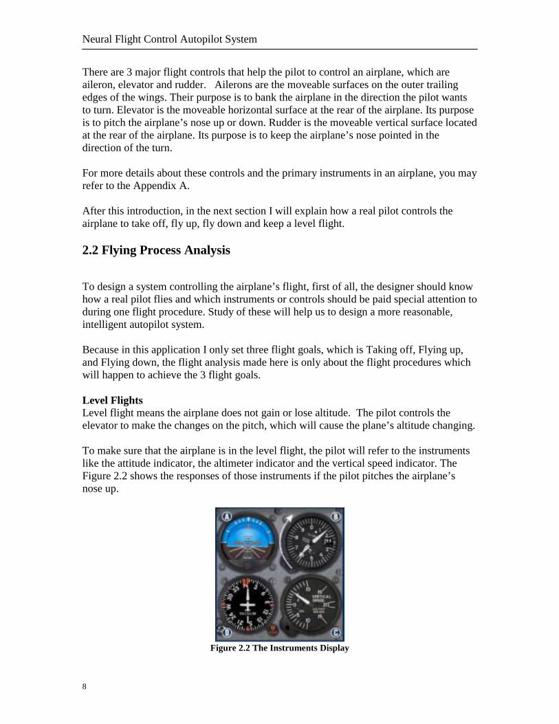
There are 3 major flight controls that help the pilot to control an airplane, which are aileron, elevator and rudder. Ailerons are the moveable surfaces on the outer trailing edges of the wings. Their purpose is to bank the airplane in the direction the pilot wants to turn. Elevator is the moveable horizontal surface at the rear of the airplane. Its purpose is to pitch the airplane’s nose up or down. Rudder is the moveable vertical surface located at the rear of the airplane. Its purpose is to keep the airplane’s nose pointed in the direction of the turn. For more details about these controls and the primary instruments in an airplane, you may refer to the Appendix A. After this introduction, in the next section I will explain how a real pilot controls the airplane to take off, fly up, fly down and keep a level flight. 2.2 Flying Process Analysis To design a system controlling the airplane’s flight, first of all, the designer should know how a real pilot flies and which instruments or controls should be paid special attention to during one flight procedure. Study of these will help us to design a more reasonable, intelligent autopilot system. Because in this application I only set three flight goals, which is Taking off, Flying up, and Flying down, the flight analysis made here is only about the flight procedures which will happen to achieve the 3 flight goals. Level Flights Level flight means the airplane does not gain or lose altitude. The pilot controls the elevator to make the changes on the pitch, which will cause the plane’s altitude changing. To make sure that the airplane is in the level flight, the pilot will refer to the instruments like the attitude indicator, the altimeter indicator and the vertical speed indicator. The Figure 2.2 shows the responses of those instruments if the pilot pitches the airplane’s nose up.
Figure 2.2 The Instruments Display
Chapter 2 Flying Analysis
9
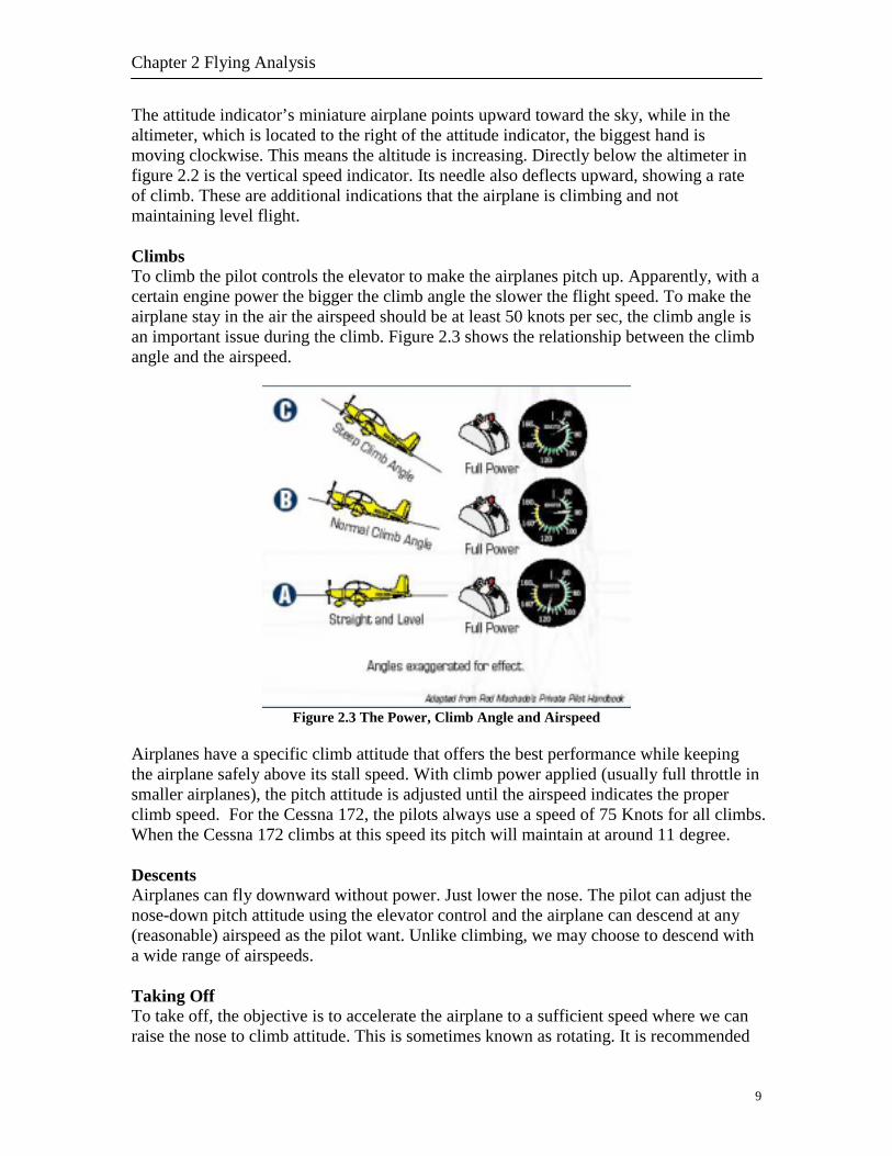
The attitude indicator’s miniature airplane points upward toward the sky, while in the altimeter, which is located to the right of the attitude indicator, the biggest hand is moving clockwise. This means the altitude is increasing. Directly below the altimeter in figure 2.2 is the vertical speed indicator. Its needle also deflects upward, showing a rate of climb. These are additional indications that the airplane is climbing and not maintaining level flight. Climbs To climb the pilot controls the elevator to make the airplanes pitch up. Apparently, with a certain engine power the bigger the climb angle the slower the flight speed. To make the airplane stay in the air the airspeed should be at least 50 knots per sec, the climb angle is an important issue during the climb. Figure 2.3 shows the relationship between the climb angle and the airspeed.
Figure 2.3 The Power, Climb Angle and Airspeed
Airplanes have a specific climb attitude that offers the best performance while keeping the airplane safely above its stall speed. With climb power applied (usually full throttle in smaller airplanes), the pitch attitude is adjusted until the airspeed indicates the proper climb speed. For the Cessna 172, the pilots always use a speed of 75 Knots for all climbs. When the Cessna 172 climbs at this speed its pitch will maintain at around 11 degree. Descents Airplanes can fly downward without power. Just lower the nose. The pilot can adjust the nose-down pitch attitude using the elevator control and the airplane can descend at any (reasonable) airspeed as the pilot want. Unlike climbing, we may choose to descend with a wide range of airspeeds. Taking Off To take off, the objective is to accelerate the airplane to a sufficient speed where we can raise the nose to climb attitude. This is sometimes known as rotating. It is recommended
Neural Flight Control Autopilot System
10
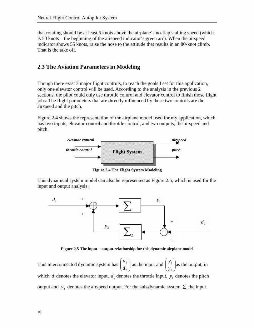
that rotating should be at least 5 knots above the airplane’s no-flap stalling speed (which is 50 knots – the beginning of the airspeed indicator’s green arc). When the airspeed indicator shows 55 knots, raise the nose to the attitude that results in an 80-knot climb. That is the take off. 2.3 The Aviation Parameters in Modeling Though there exist 3 major flight controls, to reach the goals I set for this application, only one elevator control will be used. According to the analysis in the previous 2 sections, the pilot could only use throttle control and elevator control to finish those flight jobs. The flight parameters that are directly influenced by these two controls are the airspeed and the pitch. Figure 2.4 shows the representation of the airplane model used for my application, which has two inputs, elevator control and throttle control, and two outputs, the airspeed and pitch.
elevator control airspeed throttle control pitch
Figure 2.4 The Flight System Modeling
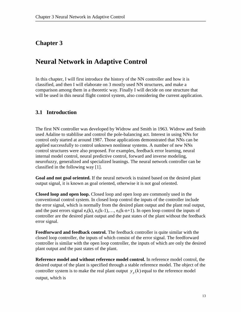
This dynamical system model can also be represented as Figure 2.5, which is used for the input and output analysis.
Figure 2.5 The input – output relationship for this dynamic airplane model
This interconnected dynamic system has
2
1
dd
as the input and
2
1
yy
as the output, in
which 1d denotes the elevator input, 2d denotes the throttle input, 1y denotes the pitch
output and 2y denotes the airspeed output. For the sub-dynamic system 1∑ the input
Flight System
∑1
1d
2d
1y
2y
+
++
+∑2

Chapter 2 Flying Analysis
11
21 yd + produces the output 1y , which means the current elevator input and current airspeed value determine the pitch value of the next time. For the sub-dynamic system
2∑ the input 12 yd + produces the output 2y , which means the current throttle input and
current pitch value determine the airspeed value of the next time. Besides of the airspeed and pitch, there are also some other parameters influenced by the throttle and the elevator, like the altitude and the vertical speed. Compared with the airspeed and pitch, those parameters are more like the indirect results of the throttle and the elevator control. For example, if the airplane is in air and pitches up, then the altitude will increase and the vertical speed will be a positive value, and vice versa. So it is better to regarded the altitude value and the vertical speed value as the references, instead of as the parameters that should be used in the system modeling. For example, when the user sets a flight order for the airplane, besides the flight action he (she) will also be asked to set the altitude the airplane should fly to; and during the flight control, the autopilot system will always check the altitude value for the flight situation analysis. Therefore, to model a flight system which is used to finished the 3 goals, I will only use 2 inputs and 2 outputs. The flight system indicates an airplane only can flight straight. The inputs are the throttle control and the elevator control, while the outputs are the airspeed value and pitch value. To control an airplane make a turn I should think about more parameters, e.g. the rudder control, the aileron control, the bank degree and etc. As explained in Appendix A.1, the ailerons control is used to bank the airplane in the direction one wants to turn, and the rudder control is used to keep the nose of the airplane pointing to the direction of turn. The airplane model then will be represented as shown in Figure 2.6.
elevator control airspeed throttle control pitch rudder control heading direction
aileron control bank degree
Figure 2.6 The Flight System Modeling
Flight System

12
Chapter 3 Neural Network in Adaptive Control
13
Chapter 3 Neural Network in Adaptive Control In this chapter, I will first introduce the history of the NN controller and how it is classified, and then I will elaborate on 3 mostly used NN structures, and make a comparison among them in a theoretic way. Finally I will decide on one structure that will be used in this neural flight control system, also considering the current application. 3.1 Introduction The first NN controller was developed by Widrow and Smith in 1963. Widrow and Smith used Adaline to stablilise and control the pole-balancing act. Interest in using NNs for control only started at around 1987. Those applications demonstrated that NNs can be applied successfully to control unknown nonlinear systems. A number of new NNs control structures were also proposed. For examples, feedback error learning, neural internal model control, neural predictive control, forward and inverse modeling, neurofuzzy, generalized and specialized leanings. The neural network controller can be classified in the following way [1]. Goal and not goal oriented. If the neural network is trained based on the desired plant output signal, it is known as goal oriented, otherwise it is not goal oriented. Closed loop and open loop. Closed loop and open loop are commonly used in the conventional control system. In closed loop control the inputs of the controller include the error signal, which is normally from the desired plant output and the plant real output, and the past errors signal es(k), es(k-1),…, es(k-n+1). In open loop control the inputs of controller are the desired plant output and the past states of the plant without the feedback error signal. Feedforward and feedback control. The feedback controller is quite similar with the closed loop controller, the inputs of which consist of the error signal. The feedforward controller is similar with the open loop controller, the inputs of which are only the desired plant output and the past states of the plant. Reference model and without reference model control. In reference model control, the desired output of the plant is specified through a stable reference model. The object of the controller system is to make the real plant output )(ky p equal to the reference model output, which is
Neural Flight Control Autopilot System
14
ε≤−∞→
||)()(||lim kyky mpk
for some specified constant 0≥ε . Direct and indirect control. In direct control the controller is trained to reduce the error between the plant and the desired output. In indirect adaptive control, it is focused on some parameters of the plant, which may not be the output of plant. The controller is trained to produce the same value on those parameters as the plant does. Hybrid and non-hybrid type. In the hybrid controller system the neural networks are used as an aid to improve the performance of some conventional controller or the fuzzy controller. In the non-hybrid control the controller system is implemented by the neural networks only. Generalized and specialized learning. When the neural network is trained to simulate the behavior of the plant in all situations, it is called generalized learning. If the neural network is trained to simulate the plant only in a special situation, it is referred to as specialized learning. Inverse and Non-inverse control. When the neural network controller performs as an inverse model of the plant, this control is referred to as inverse control. Most neural networks used for the control function are the inverse controller. To have an overview of all possible control structures, people group them into multi-levels. On the top level it is classified by the hybrid and non-hybrid classification. On the second level it is classified by the controller updating signal, which are
- Control signal - Desired output signal - Feedback controller output signal
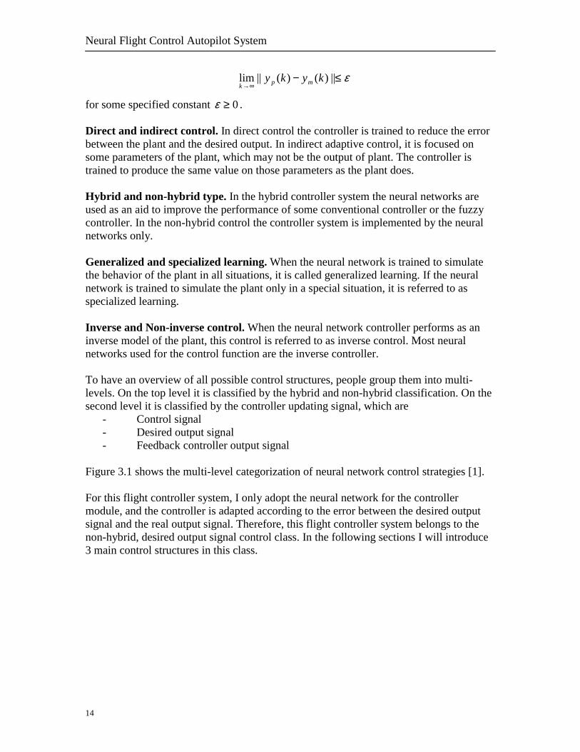
Figure 3.1 shows the multi-level categorization of neural network control strategies [1]. For this flight controller system, I only adopt the neural network for the controller module, and the controller is adapted according to the error between the desired output signal and the real output signal. Therefore, this flight controller system belongs to the non-hybrid, desired output signal control class. In the following sections I will introduce 3 main control structures in this class.
Chapter 3 Neural Network in Adaptive Control
15
Neural Predictive Control
Forward Modeling Inverse Control
Direct Inverse Control
Mimic Expert
Neural Network Control
Hybrid Non-hybrid
Control Signal Desired Output Signal Feedback Controller Signal
Indirect Learning Architecture
Mimic Conventional Controller
Feedback error Learning
NNc Plant
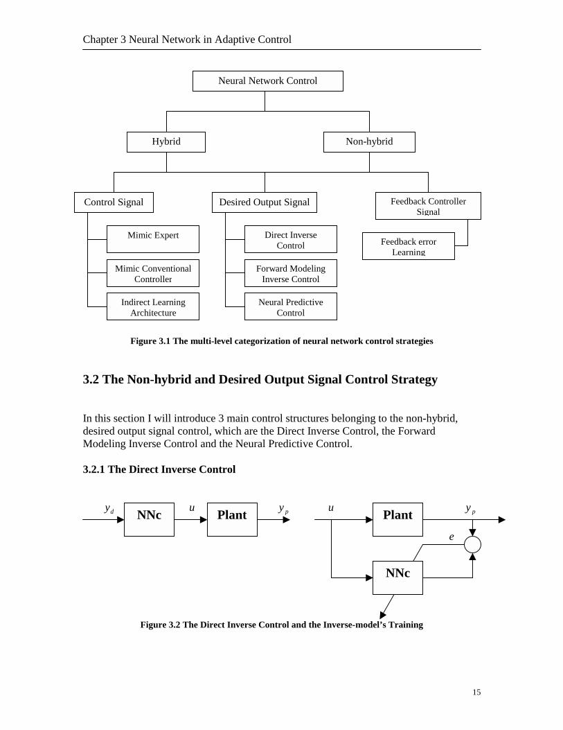
Figure 3.1 The multi-level categorization of neural network control strategies 3.2 The Non-hybrid and Desired Output Signal Control Strategy In this section I will introduce 3 main control structures belonging to the non-hybrid, desired output signal control, which are the Direct Inverse Control, the Forward Modeling Inverse Control and the Neural Predictive Control. 3.2.1 The Direct Inverse Control dy u py u py e
Figure 3.2 The Direct Inverse Control and the Inverse-model’s Training
Plant
NNc
Neural Flight Control Autopilot System
16
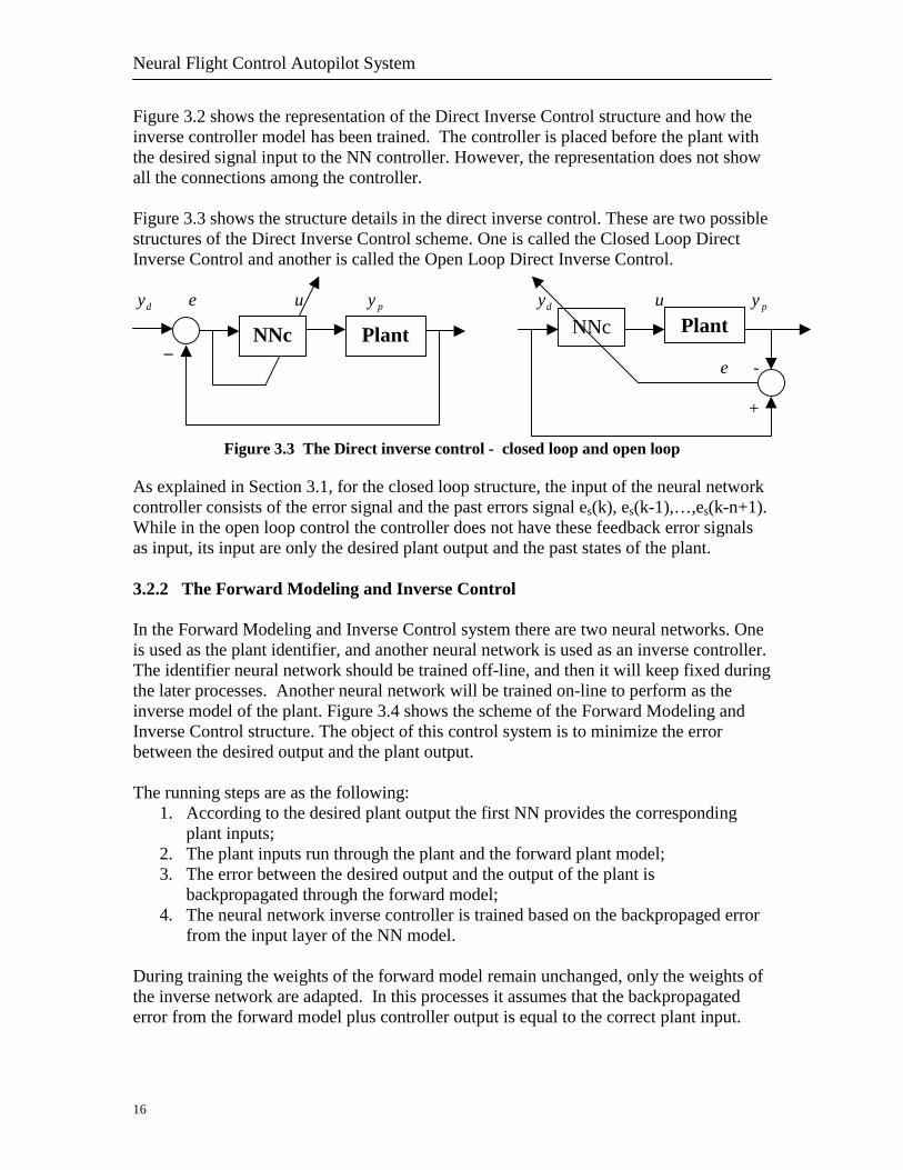
Figure 3.2 shows the representation of the Direct Inverse Control structure and how the inverse controller model has been trained. The controller is placed before the plant with the desired signal input to the NN controller. However, the representation does not show all the connections among the controller. Figure 3.3 shows the structure details in the direct inverse control. These are two possible structures of the Direct Inverse Control scheme. One is called the Closed Loop Direct Inverse Control and another is called the Open Loop Direct Inverse Control.
dy e u py dy u py _ e - +
Figure 3.3 The Direct inverse control - closed loop and open loop As explained in Section 3.1, for the closed loop structure, the input of the neural network controller consists of the error signal and the past errors signal es(k), es(k-1),…,es(k-n+1). While in the open loop control the controller does not have these feedback error signals as input, its input are only the desired plant output and the past states of the plant.
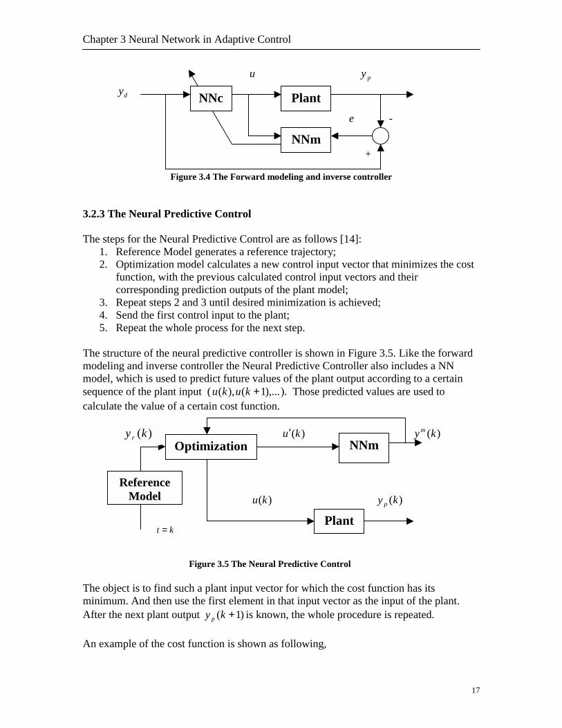
3.2.2 The Forward Modeling and Inverse Control In the Forward Modeling and Inverse Control system there are two neural networks. One is used as the plant identifier, and another neural network is used as an inverse controller. The identifier neural network should be trained off-line, and then it will keep fixed during the later processes. Another neural network will be trained on-line to perform as the inverse model of the plant. Figure 3.4 shows the scheme of the Forward Modeling and Inverse Control structure. The object of this control system is to minimize the error between the desired output and the plant output. The running steps are as the following:
1. According to the desired plant output the first NN provides the corresponding plant inputs;
2. The plant inputs run through the plant and the forward plant model; 3. The error between the desired output and the output of the plant is
backpropagated through the forward model; 4. The neural network inverse controller is trained based on the backpropaged error
from the input layer of the NN model. During training the weights of the forward model remain unchanged, only the weights of the inverse network are adapted. In this processes it assumes that the backpropagated error from the forward model plus controller output is equal to the correct plant input.
PlantNNc NNc Plant
Chapter 3 Neural Network in Adaptive Control
u py
dy e - +
Figure 3.4 The Forward modeling and inverse controller
3.2.3 The Neural Predictive Control The steps for the Neural Predictive Control are as follows [14]:
1. Reference Model generates a reference trajectory; 2. Optimization model calculates a new control input vector that minimizes the cost
function, with the previous calculated control input vectors and their corresponding prediction outputs of the plant model;
3. Repeat steps 2 and 3 until desired minimization is achieved; 4. Send the first control input to the plant; 5. Repeat the whole process for the next step.
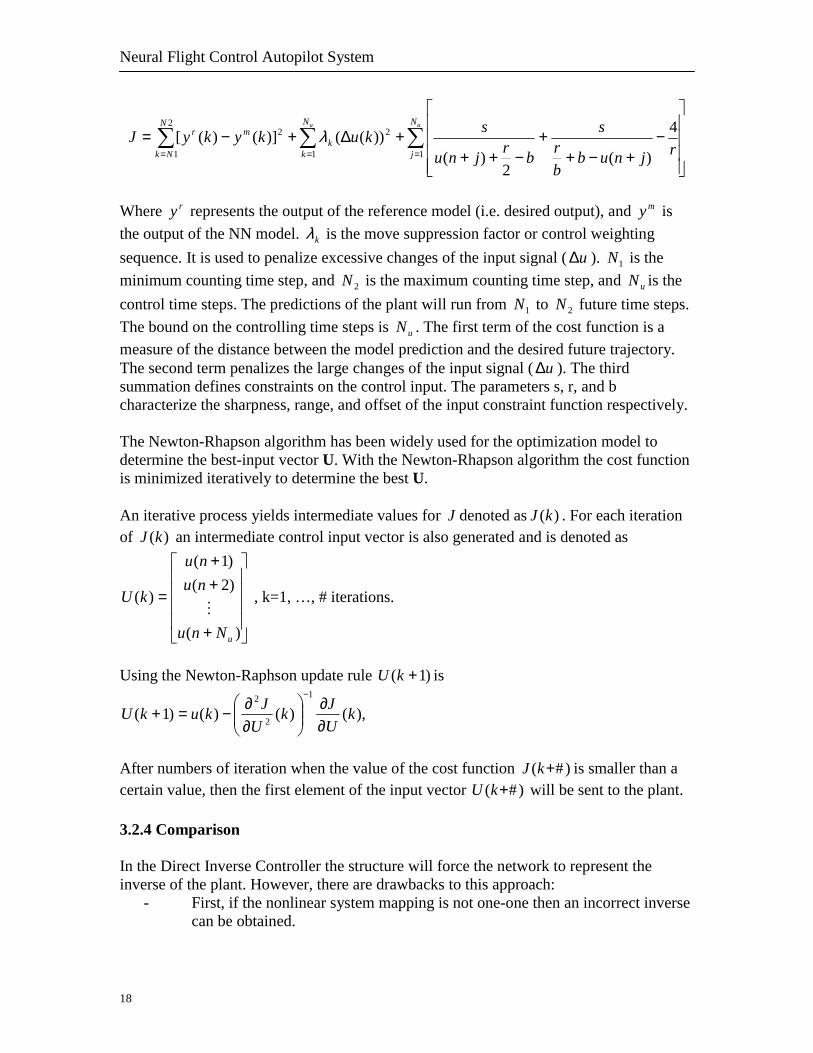
The structure of the neural predictive controller is shown in Figure 3.5. Like the forward modeling and inverse controller the Neural Predictive Controller also includes a NN model, which is used to predict future values of the plant output according to a certain sequence of the plant input ( ),...1(),( +kuku ). Those predicted values are used to calculate the value of a certain cost function.
The objeminimuAfter th An exam
Plant
NNm
NNc
)(ku ′ )(ky m
)(ku )(ky p
ct is tom. Ande next p
ple of
NNm
Plant
Optimization
Reference Model
)(kyr
17
Figure 3.5 The Neural Predictive Control
find such a plant input vector for which the cost function has its then use the first element in that input vector as the input of the plant. lant output )1( +ky p is known, the whole procedure is repeated.
the cost function is shown as following,
kt =
Neural Flight Control Autopilot System
18
∑ ∑ ∑= = =
−+−+
+−++
+∆+−=2
1 1 1
22 4
)(2
)())(()]()([
N
Nk
N
k
N
jk
mru u
rjnubbr
s
brjnu
skukykyJ λ
Where ry represents the output of the reference model (i.e. desired output), and my is the output of the NN model. kλ is the move suppression factor or control weighting sequence. It is used to penalize excessive changes of the input signal ( u∆ ). 1N is the minimum counting time step, and 2N is the maximum counting time step, and uN is the control time steps. The predictions of the plant will run from 1N to 2N future time steps. The bound on the controlling time steps is uN . The first term of the cost function is a measure of the distance between the model prediction and the desired future trajectory. The second term penalizes the large changes of the input signal ( u∆ ). The third summation defines constraints on the control input. The parameters s, r, and b characterize the sharpness, range, and offset of the input constraint function respectively. The Newton-Rhapson algorithm has been widely used for the optimization model to determine the best-input vector U. With the Newton-Rhapson algorithm the cost function is minimized iteratively to determine the best U. An iterative process yields intermediate values for J denoted as )(kJ . For each iteration of )(kJ an intermediate control input vector is also generated and is denoted as
+
++
=
)(
)2()1(
)(
uNnu
nunu
kUM
, k=1, …, # iterations.
Using the Newton-Raphson update rule )1( +kU is
),()()()1(1
2
2
kUJk
UJkukU
∂∂
∂∂−=+
−
After numbers of iteration when the value of the cost function )#( +kJ is smaller than a certain value, then the first element of the input vector )#( +kU will be sent to the plant. 3.2.4 Comparison In the Direct Inverse Controller the structure will force the network to represent the inverse of the plant. However, there are drawbacks to this approach:
- First, if the nonlinear system mapping is not one-one then an incorrect inverse can be obtained.

Chapter 3 Neural Network in Adaptive Control
19
- Second, the inversed plant models are often instable, which may lead to the instability of the whole control-system. Therefore, in the traditional control-system design it is usually avoided to adopt. Frequently, the control signal calculated by the inverse controller attains high magnitudes, so that it has to be limited before applying to the plant.
Compared with the Direct Inverse Control, the Forward Modeling and Inverse Control has an additional NN plant model, which is used in the inverse neural network training processes. The error signal is propagated back through the forward model and then the inverse model, however, only the inverse network model is adapted during this procedure. The error signal for the training algorithm in this case is the difference between the training signal and the system output (it may also be the difference between the training signal and the forward model output in the case of noisy systems, which is adopted when the real system is not viable). Jordan and Rumelhar [6] show that using the real system output can produce an exact inverse controller even when the forward model is inexact, which will not happen when the forward model output is used. In comparison with Direct Inverse Control the Forward Modeling and Inverse Control approach has the following features:
- In case where the system forward mapping is not one-one a particular inverse will still be found [6]
- Since the controller neural network gets trained assuming the correct plant input is equal to the backpropagated error from the forward model plus controller output, the training process will be stable.
Therefore, the Forward Modeling and Inverse Control could be regarded as an improved version of the direct inverse control. The Neural Predictive Controller consists of four components, a plant to be controlled, a reference model that specifies the desired performance of the plant, a neural network modeling the plant, and an optimization model used to produce the plant input vector. The object is to have an input vector for which the value of the cost function is lower than a defined value. Then the first element of the plant input for current time will be applied to the plant. In section 3.2.3 I have given an example of the cost function and the Newton-Raphson cost function minimization algorithm. The disadvantages of the Neural Predictive Control are
- Numerical minimization algorithms, e.g. Newton-Raphson, are usually very time consuming (especially if a minimum of a multivariable function has to be found), what may make them unsuitable for certain real time applications. When sampling intervals are small, there may be no time to perform minimum searching between the sampling times.

Neural Flight Control Autopilot System
20
- The prediction controller asks for a neural network model which could do a very good job to simulate the plant, since the result of the whole controller system depends on the correct prediction value. However, in some applications it could not be realized.
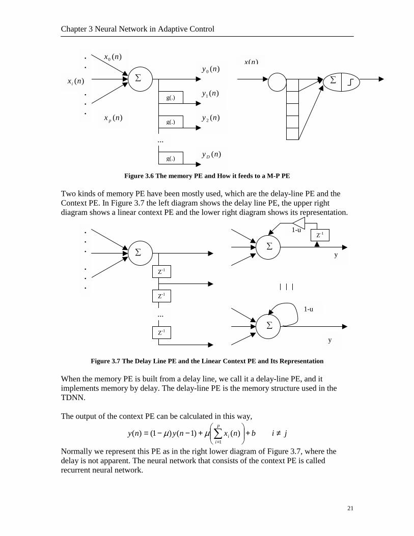
For this neural flight control system it is evaluated in the Microsoft Flight Simulator environment. While the Microsoft Flight Simulator is running, it will occupy so much CPU time, therefore the time-consuming problem should be taken very seriously here. Though there are some other optimal algorithm other than Newton-Raphson which will simplify the optimization operation, it cannot ensure that the system will work properly associated with another big program like Microsoft Flight Simulator. Moreover, in the Neural Predictive Control model a precise identifier has been asked. That is, we need to train an excellent aircraft neural network model beforehand. The problem in this application is that it is too hard to find that sets of training data covering all situations to train the aircraft NN model. However, it is not the problem for Forward modeling and inverse control. As mentioned above, Jordan and Rumelhart have showed that in the Forward Modeling and Inverse Control it can still produce an exact inverse controller even when the forward model is inexact if using the real system output to adapt the controller. On these points the Forward Modeling and Inverse Control is more suitable for this application. Therefore, I choose for the Forward Modeling and Inverse Control structure to build the control module. 3.3 Identifier The identifier is a neural network model of the plant. In this application the identifier is a neural network model of the aircraft plant. There are many topologies available to construct a neural network. Normally, to model a dynamic system people prefer to choose the time delayed topology, or the recurrent topology. In this section I will first introduce a neural component, memory PE, which makes the difference between the Time Delayed Neural Network and the Recurrent Neural Network. 3.3.1 The Memory PE Figure 3.6 shows the general structure of a memory PE and how the memory PE feeds an M-P PE. The g(.) is a delay function. The memory PE receives in general many inputs )(nxi from the previous layer, and then produces multiple outputs
[ ]TD nynyy )(),...,(0= , which are delayed versions of )(0 ny . The right diagram of the
figure 3.9 shows how the memory PE feeds a normal M-P PE. It is important to emphasize that the memory PE is a short-term memory mechanism, while the network weights represent the long-term memory of the network [3].
Chapter 3 Neural Network in Adaptive Control
21
Figure 3.6 The memory PE and How it feeds to a M-P PE Two kinds of memory PE have been mostly used, which are the delay-line PE and the Context PE. In Figure 3.7 the left diagram shows the delay line PE, the upper right diagram shows a linear context PE and the lower right diagram shows its representation.
Figure 3.7 The Delay Line PE and the Linear Context PE and Its Representation
When the memory PE is built from a delay line, we call it a delay-line PE, and it implements memory by delay. The delay-line PE is the memory structure used in the TDNN. The output of the context PE can be calculated in this way,
bnxnynyp
ii +
+−−= ∑
=1)()1()1()( µµ ji ≠
Normally we represent this PE as in the right lower diagram of Figure 3.7, where the delay is not apparent. The neural network that consists of the context PE is called recurrent neural network.
)(0 ny
)(1 ny
)(2 ny
)(nyD
)(0 nx...
.
.
.
g(.)
…
g(.)
g(.)
)(nx p
)(nxi
)(nx
∑ ∑
y
1-u ...
.
.
.
Z-1
Z-1
…
Z-1
∑∑
Z-1
∑
1-u
y
Neural Flight Control Autopilot System
22
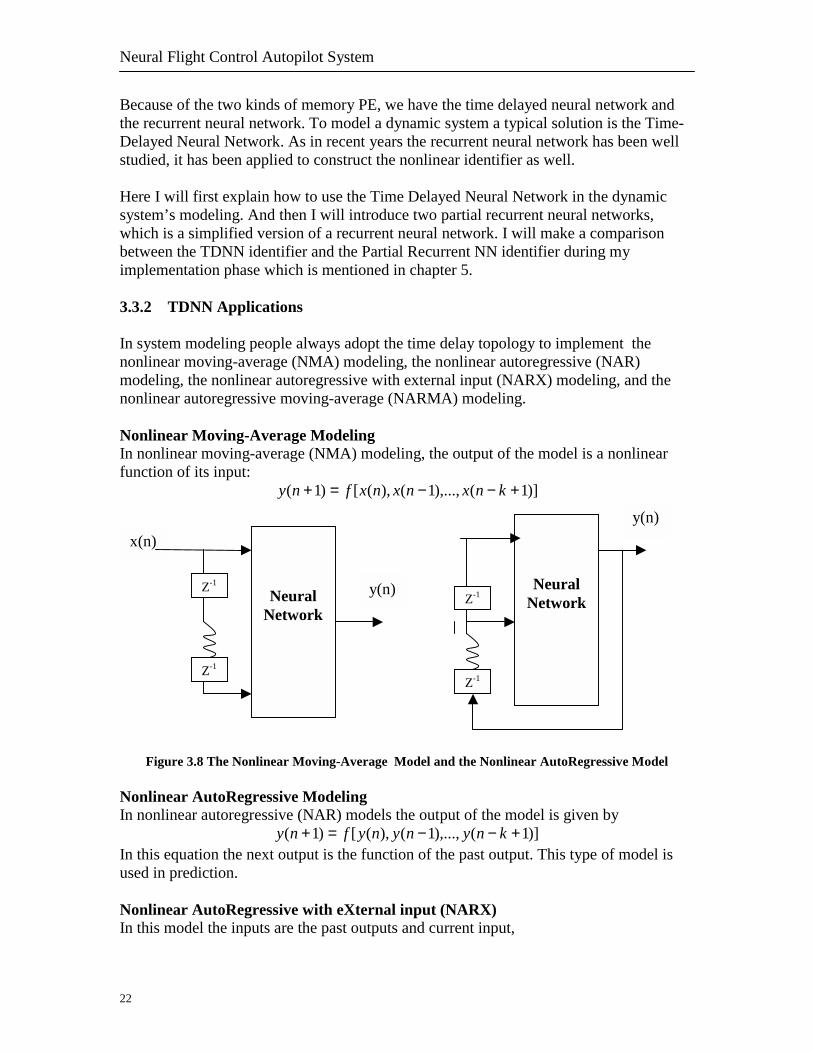
Because of the two kinds of memory PE, we have the time delayed neural network and the recurrent neural network. To model a dynamic system a typical solution is the Time-Delayed Neural Network. As in recent years the recurrent neural network has been well studied, it has been applied to construct the nonlinear identifier as well. Here I will first explain how to use the Time Delayed Neural Network in the dynamic system’s modeling. And then I will introduce two partial recurrent neural networks, which is a simplified version of a recurrent neural network. I will make a comparison between the TDNN identifier and the Partial Recurrent NN identifier during my implementation phase which is mentioned in chapter 5. 3.3.2 TDNN Applications In system modeling people always adopt the time delay topology to implement the nonlinear moving-average (NMA) modeling, the nonlinear autoregressive (NAR) modeling, the nonlinear autoregressive with external input (NARX) modeling, and the nonlinear autoregressive moving-average (NARMA) modeling. Nonlinear Moving-Average Modeling In nonlinear moving-average (NMA) modeling, the output of the model is a nonlinear function of its input:
)]1(),...,1(),([)1( +−−=+ knxnxnxfny
Figure 3.8 The Nonlinear Moving-Average Model and the Nonlinear AutoRegressive Model
Nonlinear AutoRegressive Modeling In nonlinear autoregressive (NAR) models the output of the model is given by
)]1(),...,1(),([)1( +−−=+ knynynyfny In this equation the next output is the function of the past output. This type of model is used in prediction. Nonlinear AutoRegressive with eXternal input (NARX) In this model the inputs are the past outputs and current input,
Neural
Network
x(n)
Z-1
Z-1
y(n)
Neural
Network Z-1
Z-1
y(n)
Chapter 3 Neural Network in Adaptive Control
23
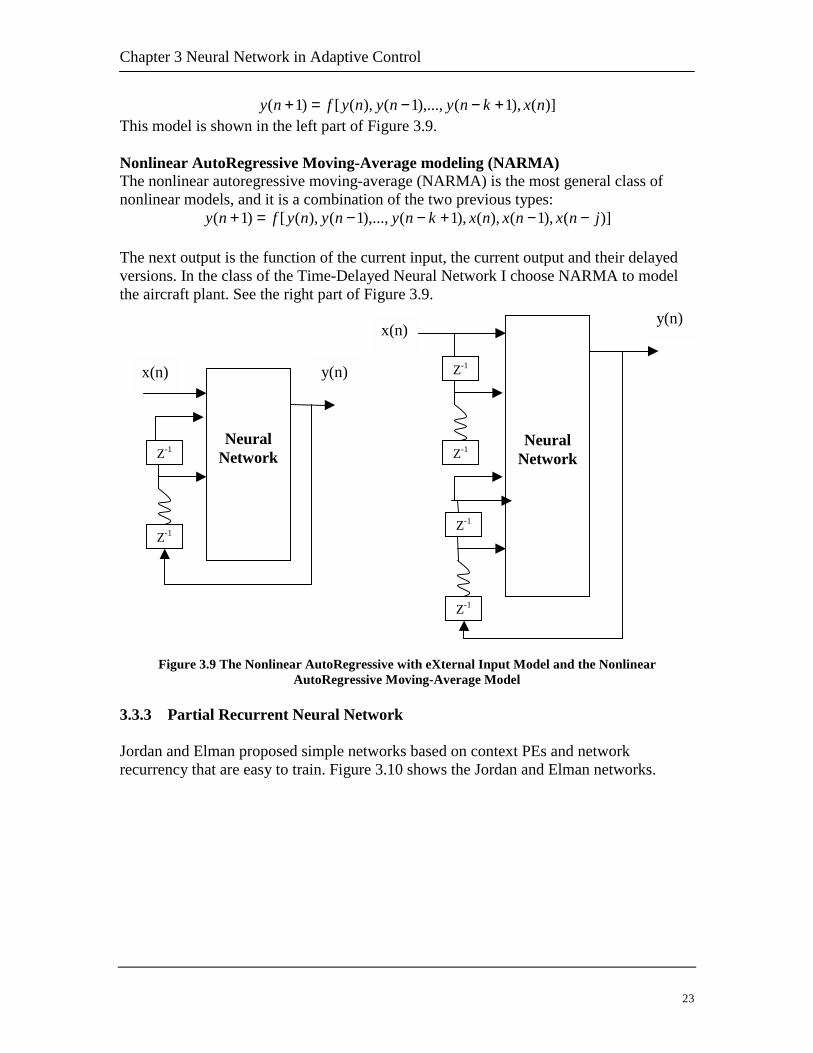
)](),1(),...,1(),([)1( nxknynynyfny +−−=+ This model is shown in the left part of Figure 3.9. Nonlinear AutoRegressive Moving-Average modeling (NARMA) The nonlinear autoregressive moving-average (NARMA) is the most general class of nonlinear models, and it is a combination of the two previous types:
)](),1(),(),1(),...,1(),([)1( jnxnxnxknynynyfny −−+−−=+ The next output is the function of the current input, the current output and their delayed versions. In the class of the Time-Delayed Neural Network I choose NARMA to model the aircraft plant. See the right part of Figure 3.9.
Figure 3.9 The Nonlinear AutoRegressive with eXternal Input Model and the Nonlinear
AutoRegressive Moving-Average Model 3.3.3 Partial Recurrent Neural Network Jordan and Elman proposed simple networks based on context PEs and network recurrency that are easy to train. Figure 3.10 shows the Jordan and Elman networks.
x(n) y(n)
x(n)y(n)
Neural Network
Z-1
Z-1
Z-1
Z-1
Neural
Network Z-1
Z-1

Neural Flight Control Autopilot System
24
BoregthesimbaJo 3.4 Boustheimimtrach
µ
11
Figure 3.10 The Jo
th the Jordan and Elman nets have fixeard the output of the context layer as e input-output path. The special architecplifies the training process. They can b
ckpropagation. Elman’s context layer rerdan’s context layer receives input from
.3 The Comparison
th TDNN and Jordan network are desiged in the nonlinear dynamic system mooretical way. I plan to compare them inplementation I have built two identifierplementing the NARMA model and anining result, finally I decide the one useapter 5.
µ
rdan and Elman network
d the feedback parameters µ and we could xternal inputs so that there is no recurrency in ture of the Jordan and Elman network e approximately trained with straight ceives input from the hidden layer, while the output.
ned to remember the past, and both of them are deling. It is hard to decide which one to use in a the practical way. Therefore, in the s, one is a time delayed neural network other one is a Jordan network. From their d in my application. I describe this process in
Chapter 4 System Design
25
Flight Plan Module
Plant
Environment
Graphic User Interface
Neural Controller Moduel
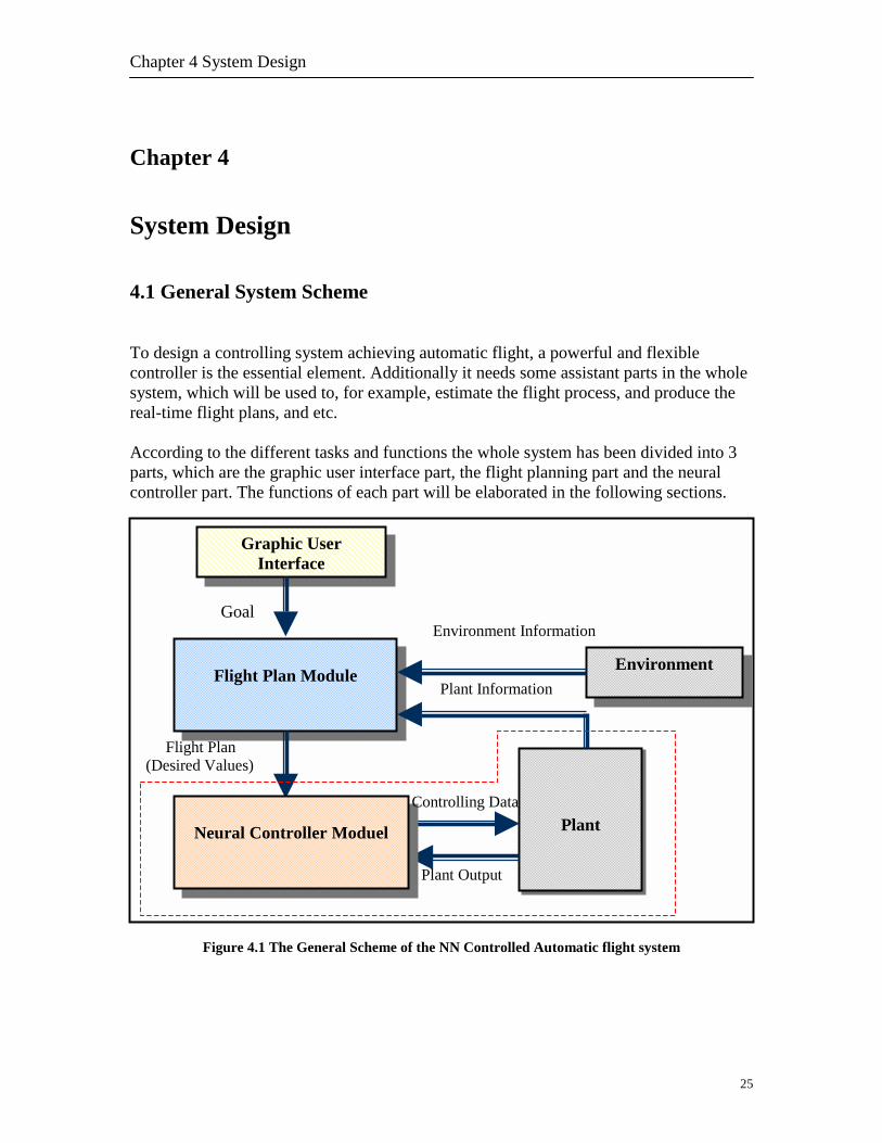
Chapter 4 System Design 4.1 General System Scheme To design a controlling system achieving automatic flight, a powerful and flexible controller is the essential element. Additionally it needs some assistant parts in the whole system, which will be used to, for example, estimate the flight process, and produce the real-time flight plans, and etc. According to the different tasks and functions the whole system has been divided into 3 parts, which are the graphic user interface part, the flight planning part and the neural controller part. The functions of each part will be elaborated in the following sections. Goal Environment Information
Plant Information
Flight Plan (Desired Values) Controlling Data
Plant Output
Figure 4.1 The General Scheme of the NN Controlled Automatic flight system
Neural Flight Control Autopilot System
26
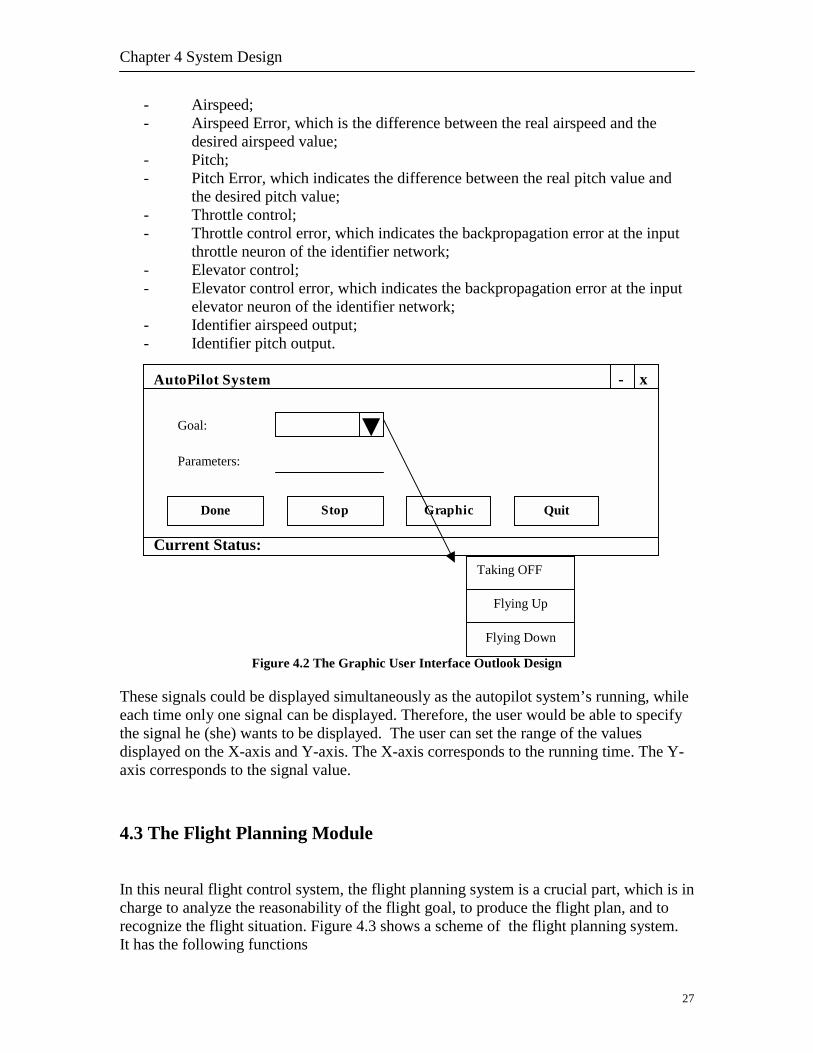
Figure 4.1 shows the general system scheme. From it you may see how the system works and see the relationship between the user interface, the flight plan and the neural controller parts. In the beginning, the user set the flight order in the user interface, e.g. Fly Up to 3000 feet, which includes the flight action and the altitude parameter. Then user interface sends this order to the flight planning system. Here the flight order will be analyzed to determine whether it is reasonable or not. If it is reasonable, the planning system will create a flight plan which may consist of several steps. Corresponding to each step the planning system will send different data to the controller module. In this case the data sent from the planning module to the controller module are the desired plant output. After receiving these desired plant output data the controller will then produce the corresponding controlling data that will finally be applied to the airplane plant. The flight planning system will also keep eye on the whole flight process, update its flight records to provide the proper plant output data. In the following sections I will elaborate these 3 modules in details. 4.2 The Graphic User Interface Through the graphic interface the user is able to set the flight order, which includes the goal and relative parameters. For example, the user could set the goal as “Taking Off”, and then set the altimeter parameters as 3000 feet. The outlook of the Graphic User Interface is shown in Figure 4.2. There is a combo control in the GUI which is used to select the flight action, and the text field under it is used to accept the parameter indicating the altitude that the airplane is expected to meet. There are also 4 buttons in the interface, done, stop, graphic, and quit. After the user presses the Done button, the interface module will send the flight goal parameter and the altitude parameter to the Flight Planning Module if both parameters are exist. The Stop button is used to stop a flight. It will reset all the parameter and reload the flight in Microsoft Flight Simulator. When the user presses the Quit button, the autopilot system will end and all the other sub-windows will also end. Before it quits from the operation system a credit window will show up. After the user click the credit window the whole autopilot system will quit. The “Graphic” function is used to visualize the evaluation data. The following signals can be displayed:
- Altitude;
Chapter 4 System Design
- Airspeed; - Airspeed Error, which is the difference between the real airspeed and the
desired airspeed value; - Pitch; - Pitch Error, which indicates the difference between the real pitch value and
the desired pitch value; - Throttle control; - Throttle control error, which indicates the backpropagation error at the input
throttle neuron of the identifier network; - Elevator control; - Elevator control error, which indicates the backpropagation error at the input
elevator neuron of the identifier network; - Identifier airspeed output; - Identifier pitch output.
Figure 4.2 The Graphic U These signals could be displayed simultaneoeach time only one signal can be displayed.the signal he (she) wants to be displayed. Tdisplayed on the X-axis and Y-axis. The X-axis corresponds to the signal value. 4.3 The Flight Planning Module In this neural flight control system, the flighcharge to analyze the reasonability of the flirecognize the flight situation. Figure 4.3 shoIt has the following functions
AutoPilot System - x Current Status:
Goal:
Parameters:
Done Stop
feet.
27
ser Interface Outlook Design
usly as the autopilot system’s running, while Therefore, the user would be able to specify he user can set the range of the values axis corresponds to the running time. The Y-
t planning system is a crucial part, which is in ght goal, to produce the flight plan, and to ws a scheme of the flight planning system.
Graphic Quit
Taking OFF
Flying Up
Flying Down

Neural Flight Control Autopilot System
28
Flight Plan Module Current Situation
Situation Recognition
Flight Plan
Data Base
Flight Plan Strategy
Goal Environment Plant
- analyzing the reasonability of the current goal; - deciding the flight plans; - providing the desired data pairs corresponding to each flight plan; - checking the current flight situation.
Current Environment Plant Information
Goal Information
Figure 4.3 The Flight Planning System Model After the user sets the desired goal and the corresponding altitude parameter in the user interface, this order will be sent to the flight planning system to analysis its reasonability, also considering the current flight situation. For example, if now the aircraft is in the taxiing procedure and the current speed is not enough to take off while the user asks to fly up immediately, after the analysis the flight planning system will ignore this order and send an error message back to let the user know this order is not possible. When the current goal has been proved reasonable and realizable, the flight plan module will then consider how to realize this goal, that is, which strategy should be carried out. For example, if the current goal is ‘Taking off’ , then the strategy center will decide to use the “Taxiing - Flying up – Default Flying” strategy instead of only the Taxiing or only the Flying up strategy. For each flight procedure the flight plan module will produce the corresponding desired plant output data pairs, which will be in the next module, the neural network controller module. In this application I have set 3 flight goals, which are the ‘Taking Off”, “Flying Up”, and “Flying Down”. The 3 flight goals include different flight procedures. For example, for
Desired Plant Output
Chapter 4 System Design
29
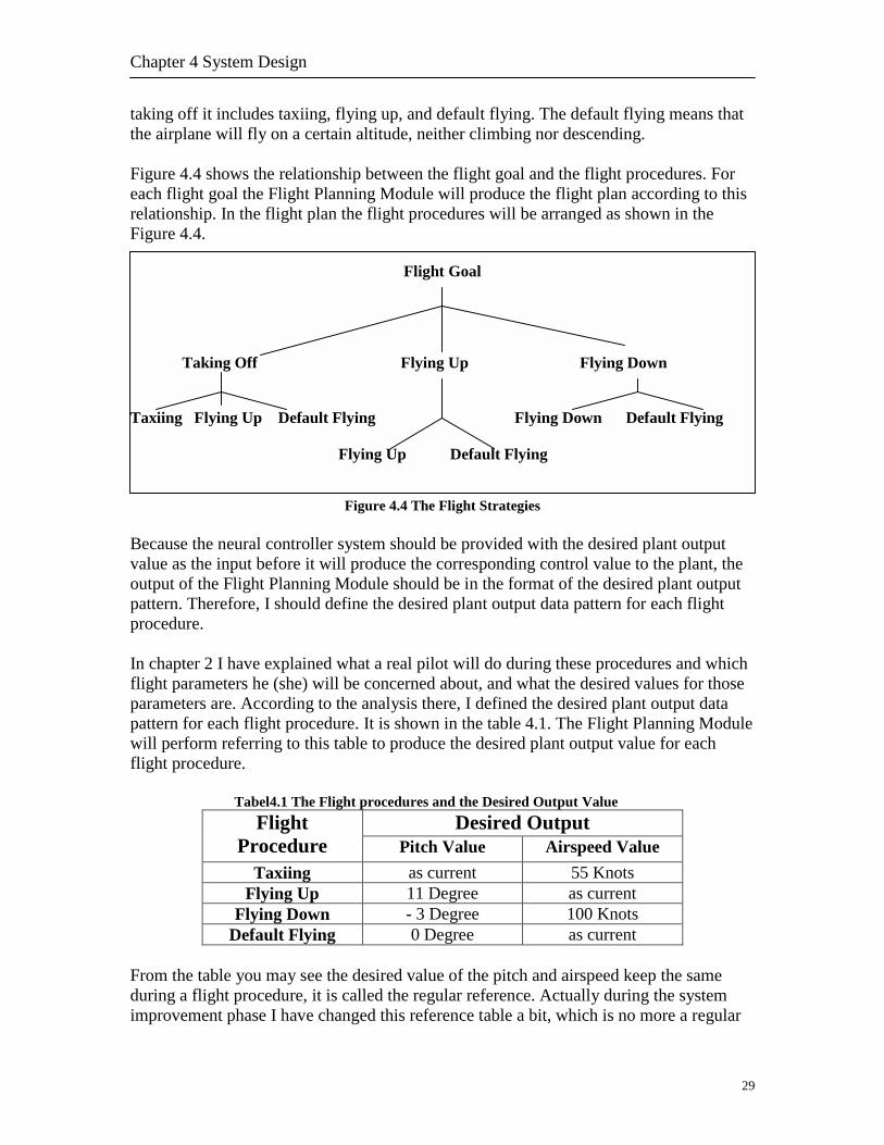
taking off it includes taxiing, flying up, and default flying. The default flying means that the airplane will fly on a certain altitude, neither climbing nor descending. Figure 4.4 shows the relationship between the flight goal and the flight procedures. For each flight goal the Flight Planning Module will produce the flight plan according to this relationship. In the flight plan the flight procedures will be arranged as shown in the Figure 4.4.
Flight Goal Taking Off Flying Up Flying Down Taxiing Flying Up Default Flying Flying Down Default Flying
Flying Up Default Flying
Figure 4.4 The Flight Strategies
Because the neural controller system should be provided with the desired plant output value as the input before it will produce the corresponding control value to the plant, the output of the Flight Planning Module should be in the format of the desired plant output pattern. Therefore, I should define the desired plant output data pattern for each flight procedure. In chapter 2 I have explained what a real pilot will do during these procedures and which flight parameters he (she) will be concerned about, and what the desired values for those parameters are. According to the analysis there, I defined the desired plant output data pattern for each flight procedure. It is shown in the table 4.1. The Flight Planning Module will perform referring to this table to produce the desired plant output value for each flight procedure.
Tabel4.1 The Flight procedures and the Desired Output Value Desired Output Flight
Procedure Pitch Value Airspeed Value Taxiing as current 55 Knots
Flying Up 11 Degree as current Flying Down - 3 Degree 100 Knots
Default Flying 0 Degree as current From the table you may see the desired value of the pitch and airspeed keep the same during a flight procedure, it is called the regular reference. Actually during the system improvement phase I have changed this reference table a bit, which is no more a regular
Neural Flight Control Autopilot System
30
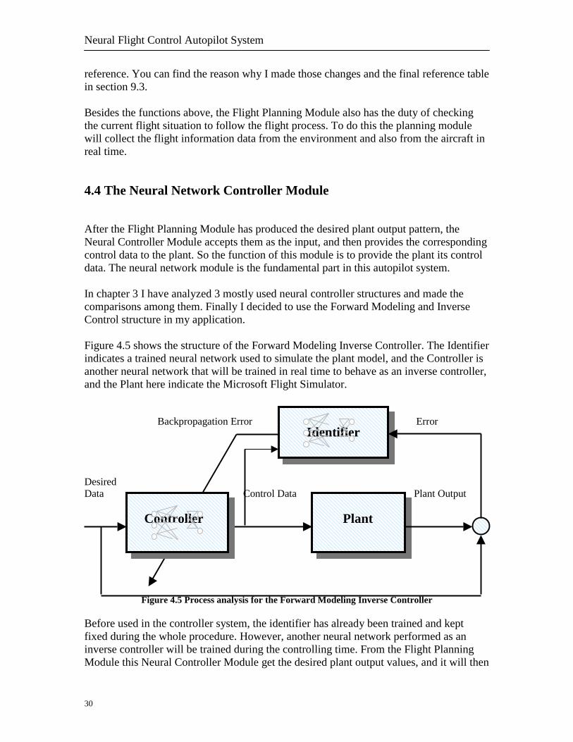
reference. You can find the reason why I made those changes and the final reference table in section 9.3. Besides the functions above, the Flight Planning Module also has the duty of checking the current flight situation to follow the flight process. To do this the planning module will collect the flight information data from the environment and also from the aircraft in real time. 4.4 The Neural Network Controller Module After the Flight Planning Module has produced the desired plant output pattern, the Neural Controller Module accepts them as the input, and then provides the corresponding control data to the plant. So the function of this module is to provide the plant its control data. The neural network module is the fundamental part in this autopilot system. In chapter 3 I have analyzed 3 mostly used neural controller structures and made the comparisons among them. Finally I decided to use the Forward Modeling and Inverse Control structure in my application. Figure 4.5 shows the structure of the Forward Modeling Inverse Controller. The Identifier indicates a trained neural network used to simulate the plant model, and the Controller is another neural network that will be trained in real time to behave as an inverse controller, and the Plant here indicate the Microsoft Flight Simulator. Backpropagation Error Error
Desired Data Control Data Plant Output
Figure 4.5 Process analysis for the Forward Modeling Inverse Controller Before used in the controller system, the identifier has already been trained and kept fixed during the whole procedure. However, another neural network performed as an inverse controller will be trained during the controlling time. From the Flight Planning Module this Neural Controller Module get the desired plant output values, and it will then
Plant
Identifier
Controller
Chapter 4 System Design
31
produce the corresponding control data. The control data will be sent to the plant to control the aircraft and also be sent to the identifier. According to the error between the real plant output and the desired plant output value the neural controller will be trained then.

32
Chapter 5 Module Specification
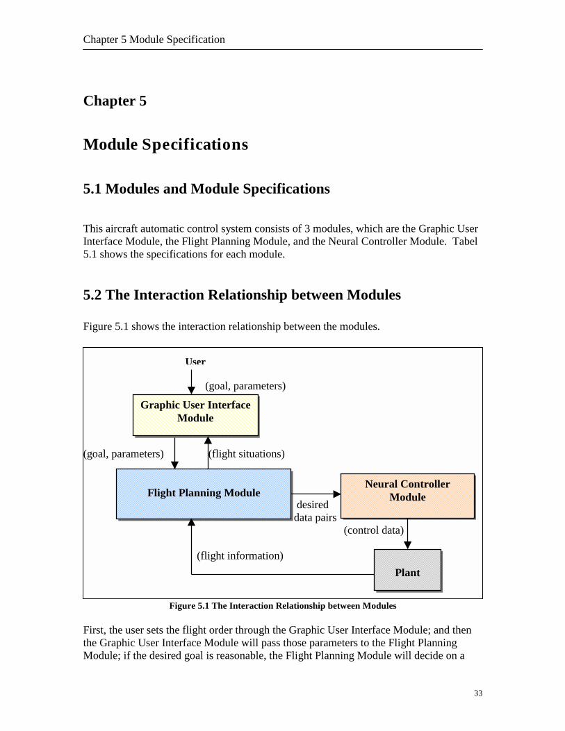
Chapter 5 Module Specifications 5.1 Modules and Module Specifications This aircraft automatic control system consists of 3 modules, which are the Graphic User Interface Module, the Flight Planning Module, and the Neural Controller Module. Tabel 5.1 shows the specifications for each module. 5.2 The Interaction Relationship between Modules Figure 5.1 shows the interaction relationship between the modules. (goal, parameters)
Fig First, the user sets thethe Graphic User InteModule; if the desired
Flight
GraphicM
User
33
(goal, parameters)
(flight situations)
desired
data pairs (control data) (flight information)
ure 5.1 The Interaction Relationship between Modules
flight order through the Graphic User Interface Module; and then rface Module will pass those parameters to the Flight Planning goal is reasonable, the Flight Planning Module will decide on a
Neural Controller Module Planning Module
User Interface odule
Plant
Neural Flight Control Autopilot System
34
flight plan and continuously provide the desired plant output pairs to the Neural Controller Module. The Flight Planning Module will follow the flight process and return current flight situation to Graphic User Interface Module. For each desired plant output patterns received from the Flight Planning Module the Neural Controller Module will produce the control data applied to the plant.
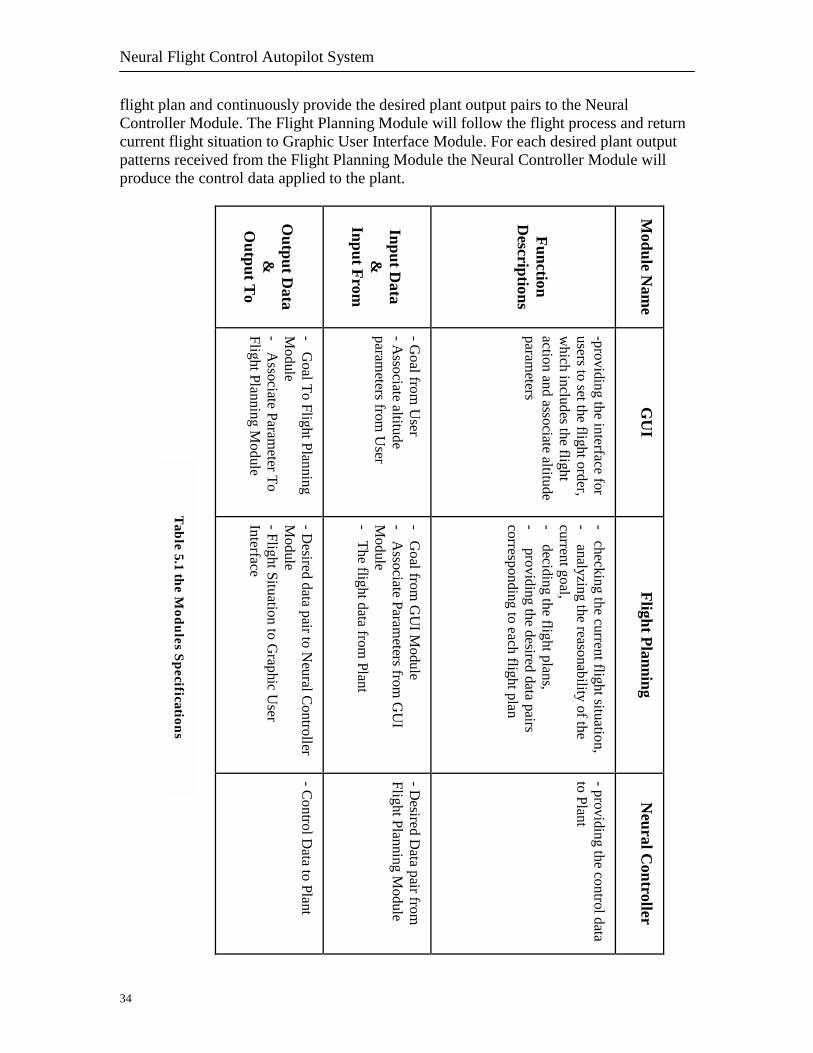
O
utput Data
&
Output T
o
Input D
ata &
Input From
Function
Descriptions
Module N
ame
- Goal To Flight Planning
Module
- Associate Param
eter To Flight Planning M
odule
- Goal from
User
- Associate altitude
parameters from
User
-providing the interface for users to set the flight order, w
hich includes the flight action and associate altitude param
eters GU
I
- Desired data pair to N
eural Controller
Module
- Flight Situation to Graphic U
ser Interface
- Goal from
GU
I Module
- Associate Param
eters from G
UI
Module
- The flight data from Plant
- checking the current flight situation, - analyzing the reasonability of the current goal, - deciding the flight plans, - providing the desired data pairs corresponding to each flight plan
Flight Planning
- Control D
ata to Plant
- Desired D
ata pair from
Flight Planning Module
- providing the control data to Plant
Neural C
ontroller
Table 5.1 the Modules Specifications

Chapter 5 Module Specification
5.3 The Server-Client Structure The interaction diagram only shows the function relationships without explaining how they collaborate in time. During the working process, the user can set the goal at any time no matter whether or not the Flight Planning Module and the Neural Controller Module is working on the current goal, the Flight Planning Module will accept the new goal and analyze its reasonability, while in the mean time it may be still providing the Neural Controller Module the desired data pairs for the current flight procedure. If the new goal is reasonable the Flight Planning Module will stop the current control process and start another process working on the new goal and set it as the current goal. If the new goal is not reasonable the Flight Planning Module will continue current controlling process and wait for another goal from the user. Therefore, the working structure of this system is more like a server-client structure. The user and the GUI module represent the client part which sends the requests to the server program and the Flight Planning Module represents the server program which accept the clients’ request and decide which one will be processed. In one time there is only one request that will be accepted and be processed. Figure 5.2 shows this server-client structure. Client
Figure 5.2 The
Flight P
NN M
GU
Server
User
35
server-client structure analysis
lanning Module
Controller odule Plant
I Module

36
37
Part II
System Implementation

38

Chapter 6 Neural Controller Module Implementation
39
Chapter 6 Neural Controller Module Implementation 6.1 Process Analysis and Flow Chart After the analysis and design I will now discuss the implementation. In this chapter first I will analysis the modules’ working processes in detail, and then draw a flow char. All the programs are written in Visual C++ 6.0 environment and in C language. Figure 6.1 shows the structure of the Forward Modeling Inverse Controller marked on the process steps and the transferring data. Here, the Identifier indicates a neural network trained as the plant model, and the Controller is another neural network that will be trained in real time, and the Plant here indicates the Microsoft Flight Simulator. Backpropagation Error 8 7 Error
3
Desired 9 Data Control Data Plant Output 1 2 4 5 6
Figure 6.1 The Process analysis for the Forward Modeling Inverse Controller During the whole process,
- Step 1 is to propagate a desired output pattern through the neural controller; - Step 2 is to get the control data out of the corresponding neural controller for
that desired value pattern; - Step 3 is to propagate the control data pattern through the neural identifier; - Step 4 is to send the control data to the plant; - Step 5 is to read out the real output value from the plant; - Step 6 is to get the error between the real output values and the desired values; - Step 7and 8 is to backpropagate the error through neural identifier, and then
get the corresponding error at the input layer;
Plant
Identifier
Controller
Neural Flight Control Autopilot System
40
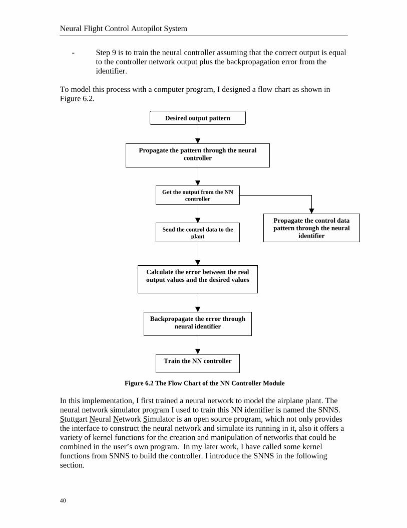
- Step 9 is to train the neural controller assuming that the correct output is equal to the controller network output plus the backpropagation error from the identifier.
To model this process with a computer program, I designed a flow chart as shown in Figure 6.2.
Figure 6.2 The Flow Chart of the NN Controller Module In this implementation, I first trained a neural network to model the airplane plant. The neural network simulator program I used to train this NN identifier is named the SNNS. Stuttgart Neural Network Simulator is an open source program, which not only provides the interface to construct the neural network and simulate its running in it, also it offers a variety of kernel functions for the creation and manipulation of networks that could be combined in the user’s own program. In my later work, I have called some kernel functions from SNNS to build the controller. I introduce the SNNS in the following section.
Desired output pattern
Propagate the pattern through the neural controller
Get the output from the NN controller
Propagate the control data pattern through the neural
identifier Send the control data to the
plant
Calculate the error between the real output values and the desired values
Backpropagate the error through neural identifier
Train the NN controller
Chapter 6 Neural Controller Module Implementation
41
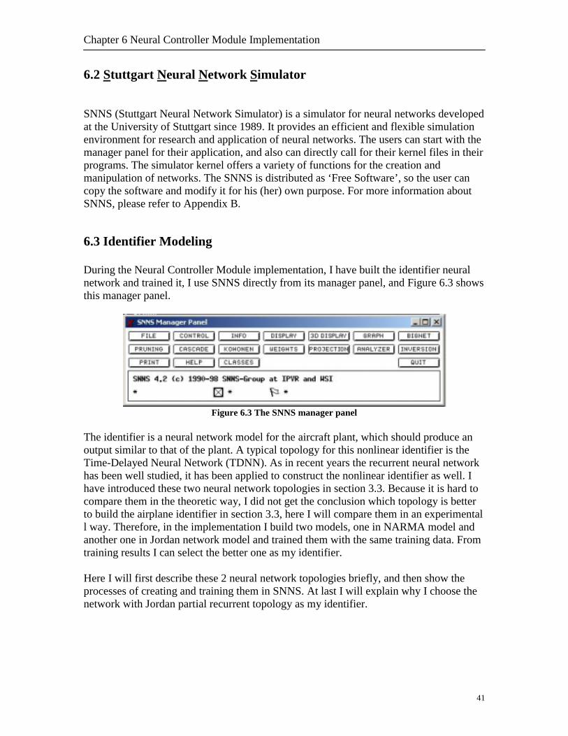
6.2 Stuttgart Neural Network Simulator SNNS (Stuttgart Neural Network Simulator) is a simulator for neural networks developed at the University of Stuttgart since 1989. It provides an efficient and flexible simulation environment for research and application of neural networks. The users can start with the manager panel for their application, and also can directly call for their kernel files in their programs. The simulator kernel offers a variety of functions for the creation and manipulation of networks. The SNNS is distributed as ‘Free Software’, so the user can copy the software and modify it for his (her) own purpose. For more information about SNNS, please refer to Appendix B. 6.3 Identifier Modeling During the Neural Controller Module implementation, I have built the identifier neural network and trained it, I use SNNS directly from its manager panel, and Figure 6.3 shows this manager panel.
Figure 6.3 The SNNS manager panel
The identifier is a neural network model for the aircraft plant, which should produce an output similar to that of the plant. A typical topology for this nonlinear identifier is the Time-Delayed Neural Network (TDNN). As in recent years the recurrent neural network has been well studied, it has been applied to construct the nonlinear identifier as well. I have introduced these two neural network topologies in section 3.3. Because it is hard to compare them in the theoretic way, I did not get the conclusion which topology is better to build the airplane identifier in section 3.3, here I will compare them in an experimental l way. Therefore, in the implementation I build two models, one in NARMA model and another one in Jordan network model and trained them with the same training data. From training results I can select the better one as my identifier. Here I will first describe these 2 neural network topologies briefly, and then show the processes of creating and training them in SNNS. At last I will explain why I choose the network with Jordan partial recurrent topology as my identifier.

Neural Flight Control Autopilot System
42
6.3.1 NARMA vs. Jordan Network The nonlinear autoregressive moving-average (NARMA) is the most general class of nonlinear models, which can be represented as following,
)](),1(),(),1(),...,1(),([)1( jnxnxnxknynynyfny −−+−−=+ That is, we drive TDNN with its past outputs and also with the input and its delayed versions. See the left figure in Figure 6.4. Jordan network is based on context PEs. The feed back parameters µ are fixed. Its topology is shown in the right part of Figure 6.4.
Figure 6.4 The NARMA Model and the Jordan Network Model
6.3.2 Identifiers’ Constructing Referring to the analysis in chapter 2, for this identifier it only has 4 input-output parameters. The input parameters are the elevator control and the throttle control, and the output parameters are the pitch value and the airspeed value. Using SNNS I first built two neural networks respectively in the NARMA topology and the Jordan network topology. Based on the preliminary experience, I have already come to the conclusion that for an identifier whose input and output relationship is not so complex one hidden layer with around 20 neurons is enough. Of course, one can construct a multi hidden layer neural network with each hidden layer having around 12 neurons. However, it will not help so much, but only waste time in training. Therefore, in this application both in the NARMA network and in the Jordan network I set only one hidden layer. After deciding the neural network’s structure and the layer, I constructed them in SNNS. The panel used to construct a time delayed neural network is shown in the left part of Figure 6.5, and the panel shown in the right part of the Figure 6.5 is used to construct the Jordan network.
µ
1
x(n) y(n)
NeuralNetwork
Z-1
Z-1
Z-1
Z-1

Chapter 6 Neural Controller Module Implementation
43
Figure 6.5 The management panel for TDNN and Jordan Network in SNNS The time-delayed length for the TDNN is set to 5. Figure 6.6 shows this 5 time-delayed NARMA neural network and the Jordan network.
Figure 6.6 The 5 time-delayed NARMA neural network and Jordan Network
Neural Flight Control Autopilot System
44
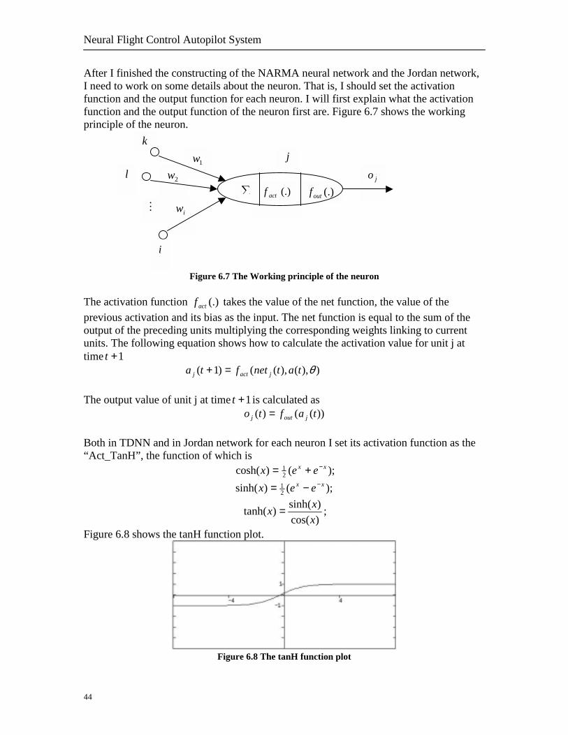
After I finished the constructing of the NARMA neural network and the Jordan network, I need to work on some details about the neuron. That is, I should set the activation function and the output function for each neuron. I will first explain what the activation function and the output function of the neuron first are. Figure 6.7 shows the working principle of the neuron.
Figure 6.7 The Working principle of the neuron
The activation function (.)actf takes the value of the net function, the value of the previous activation and its bias as the input. The net function is equal to the sum of the output of the preceding units multiplying the corresponding weights linking to current units. The following equation shows how to calculate the activation value for unit j at time 1+t
)),(),(()1( θtatnetfta jactj =+ The output value of unit j at time 1+t is calculated as
))(()( tafto joutj = Both in TDNN and in Jordan network for each neuron I set its activation function as the “Act_TanH”, the function of which is
);()cosh( 21 xx eex −+=
);()sinh( 21 xx eex −−=
)cos()sinh()tanh(
xxx = ;
Figure 6.8 shows the tanH function plot.
Figure 6.8 The tanH function plot
jo
k
iw
2w1w
(.)outf∑ (.)actf
…
jl
i
Chapter 6 Neural Controller Module Implementation
45
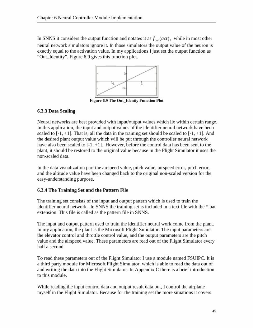
In SNNS it considers the output function and notates it as )(actfout , while in most other neural network simulators ignore it. In those simulators the output value of the neuron is exactly equal to the activation value. In my applications I just set the output function as “Out_Identity”. Figure 6.9 gives this function plot.
Figure 6.9 The Out_Identiy Function Plot
6.3.3 Data Scaling Neural networks are best provided with input/output values which lie within certain range. In this application, the input and output values of the identifier neural network have been scaled to [-1, +1]. That is, all the data in the training set should be scaled to [-1, +1]. And the desired plant output value which will be put through the controller neural network have also been scaled to [-1, +1]. However, before the control data has been sent to the plant, it should be restored to the original value because in the Flight Simulator it uses the non-scaled data. In the data visualization part the airspeed value, pitch value, airspeed error, pitch error, and the altitude value have been changed back to the original non-scaled version for the easy-understanding purpose. 6.3.4 The Training Set and the Pattern File The training set consists of the input and output pattern which is used to train the identifier neural network. In SNNS the training set is included in a text file with the *.pat extension. This file is called as the pattern file in SNNS. The input and output pattern used to train the identifier neural work come from the plant. In my application, the plant is the Microsoft Flight Simulator. The input parameters are the elevator control and throttle control value, and the output parameters are the pitch value and the airspeed value. These parameters are read out of the Flight Simulator every half a second. To read these parameters out of the Flight Simulator I use a module named FSUIPC. It is a third party module for Microsoft Flight Simulator, which is able to read the data out of and writing the data into the Flight Simulator. In Appendix C there is a brief introduction to this module. While reading the input control data and output result data out, I control the airplane myself in the Flight Simulator. Because for the training set the more situations it covers

Neural Flight Control Autopilot System
4
the better the training result will be, I try not to make a straight and level flight during the process. To make sure that the frequency in which I read the data out of the Flight Simulator is sufficient, I wrote a program to write these input and output pattern data into the Flight Simulator through the FSUIPC module in the same frequency. As the flight behavior is exactly the same as before I flied, I can make sure the frequency I choose to read the data out is sufficient. To train the neural networks, I have created 2 training sets for each of them. One is used in training, and another one is used in the validation. The training sets used for the Jordan network include 400 patterns each. The training sets used for TDNN include 396 patterns each. In SNNS the training set is represented in a pattern file. The pattern file has its own structure. Figure 6.10 shows an example of the header of the pattern file, which will indicate the number of the training patterns and the number of input and output parameters.
Tawf
SNNS pattern definition file V1.4generated at Fri Nov 07 08:57:27 2003 No. of patterns: 400 No. of input units: 20 No. of output units: 2
Figure 6.10 An Example of the Pattern File with Header
he contents of the pattern file are the input and output patterns, which are also written in special format. For each pattern, it starts with the input parameter, and then followed ith the output parameters. Figure 6.11 shows an example of the contents of the pattern
ile for the Jordan network.
# Input pattern 1:0.000000 0.000000 # Output pattern 1: 0.000000 -0.101089 # Input pattern 2: 0.000000 0.000000 # Output pattern 2: 0.000000 -0.101089 … …
6
Figure 6.11 An Example of the Pattern File with Contents
Chapter 6 Neural Controller Module Implementation
47
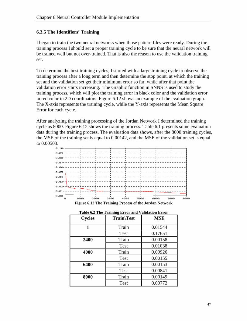
6.3.5 The Identifiers’ Training I began to train the two neural networks when those pattern files were ready. During the training process I should set a proper training cycle to be sure that the neural network will be trained well but not over-trained. That is also the reason to use the validation training set. To determine the best training cycles, I started with a large training cycle to observe the training process after a long term and then determine the stop point, at which the training set and the validation set get their minimum error so far, while after that point the validation error starts increasing. The Graphic function in SNNS is used to study the training process, which will plot the training error in black color and the validation error in red color in 2D coordinators. Figure 6.12 shows an example of the evaluation graph. The X-axis represents the training cycle, while the Y-axis represents the Mean Square Error for each cycle. After analyzing the training processing of the Jordan Network I determined the training cycle as 8000. Figure 6.12 shows the training process. Table 6.1 presents some evaluation data during the training process. The evaluation data shows, after the 8000 training cycles, the MSE of the training set is equal to 0.00142, and the MSE of the validation set is equal to 0.00503.
Figure 6.12 The Training Process of the Jordan Network
Table 6.2 The Training Error and Validation Error Cycles Train\Test MSE
Train 0.01544 1 Test 0.17651 Train 0.00158 2400 Test 0.01038 Train 0.00926 4000 Test 0.00155 Train 0.00153 6400 Test 0.00841 Train 0.00149 8000 Test 0.00772

Neural Flight Control Autopilot System
48
For TDNN I set the training cycle to 800. Figure 6.13 shows this training process. Table 6.2 presents some evaluation data during the training process. The evaluation data shows, after the 800 training cycles, the MSE of the training set is equal to 0.00149, and the MSE of the validation set is equal to 0.00534.
Figure 6.13 The Training Process of the TDNN
Table 6.2 The Training Error and Validation Error Cycles Train\Test MSE
Train 0.02911 1 Test 0.08965 Train 0.00207 240 Test 0.00711 Train 0.71387 400 Test 0.00864 Train 0.00157 620 Test 0.00790 Train 0.00149 800 Test 0.00534
6.3.6 Comparisons The training result shows that for this Jordan network identifier and this 5-delayed TDNN identifier they have the same ability to model the airplane plant, because at last the MSE of the training set is around 0.00149. However, the 5-delayed TDNN has much shorter training cycles than the Jordan network, which is 8000: 800. When the Jordan network has been trained 800 cycles, the MSE of the training set is around 0.00194. The advantage of the Jordan network is the simpler structure. Because of this for a single training cycle it needs a shorter training time. In the Feed Forward and Inverse neural network controller, except the pre-trained neural network identifier, there is another neural network performed as an inverse controller which normally has the same structure as the identifier. This controller neural network will be trained in real time. The Jordan network identifier has the same quality as the NARMA identifier to model the airplane plant, while the Jordan network has a simpler
Chapter 6 Neural Controller Module Implementation
49
structure which makes it more suitable for real time training, therefore, I choose the Jordan network structure both for the identifier and the inversed neural network controller. 6.4 The Controller Module Programming After training the aircraft identifier, I continued implementing this controller module. Referring to the flow chart I have drawn in section 6.2, I have written the programs for each running step, and then combined them together. In this procedure, I also call some kernel functions from SNNS kernel files. In Appendix D I list those programs used for each step. What should be mentioned here is that the controller neural network in this module is also built with the Jordan network. It will be trained in real time, while the identifier has kept unchanged all the time.
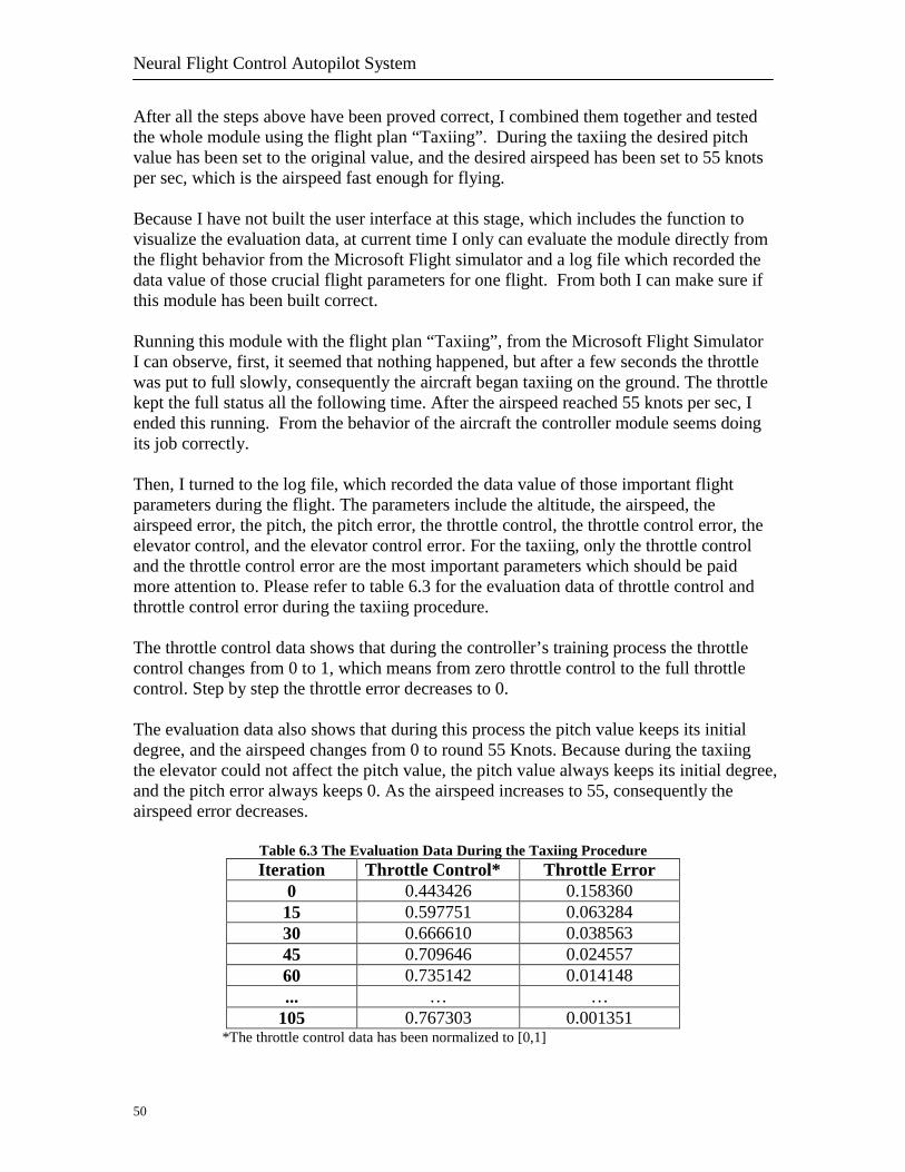
6.5 Module Test During the programming, for each step I have performed a test. For example, in step 1 and step 2, I have to propagate the data pair through the neural network and get the output result from network. To test I compared the result from my program with the result from the SNNS after loading the same network and the same input. If they are the same, it means my program is correct. In step 4 and step 5, I have to write the data into the Flight Simulator and read the data from the Flight Simulator, since I have already used those functions before (in the getting training set process), they should be correct here. In step 7 and 8, I have to backpropagate the error through the neural identifier, and then to get the corresponding error at the input layer. What I have done for the testing was repeating the evaluations several times with different error value as the input, and then comparing the output of the functions. If those outputs had a reasonable trend, then I would presume the function I have written was correct. For example, as the error increases the absolute value of the backpropagation error should also increase. In step 9, I have to train the neural controller based on single data pattern. I used the same neural network and the same pattern data both in my program and in the SNNS, and then set the same learning parameter, λ , and asked them to learn in the same cycles. After this was finished, I propagated the same pattern through the neural network both in my program and in SNNS. From the output value of the network I made sure my program was correct.
Neural Flight Control Autopilot System
50
After all the steps above have been proved correct, I combined them together and tested the whole module using the flight plan “Taxiing”. During the taxiing the desired pitch value has been set to the original value, and the desired airspeed has been set to 55 knots per sec, which is the airspeed fast enough for flying. Because I have not built the user interface at this stage, which includes the function to visualize the evaluation data, at current time I only can evaluate the module directly from the flight behavior from the Microsoft Flight simulator and a log file which recorded the data value of those crucial flight parameters for one flight. From both I can make sure if this module has been built correct. Running this module with the flight plan “Taxiing”, from the Microsoft Flight Simulator I can observe, first, it seemed that nothing happened, but after a few seconds the throttle was put to full slowly, consequently the aircraft began taxiing on the ground. The throttle kept the full status all the following time. After the airspeed reached 55 knots per sec, I ended this running. From the behavior of the aircraft the controller module seems doing its job correctly. Then, I turned to the log file, which recorded the data value of those important flight parameters during the flight. The parameters include the altitude, the airspeed, the airspeed error, the pitch, the pitch error, the throttle control, the throttle control error, the elevator control, and the elevator control error. For the taxiing, only the throttle control and the throttle control error are the most important parameters which should be paid more attention to. Please refer to table 6.3 for the evaluation data of throttle control and throttle control error during the taxiing procedure. The throttle control data shows that during the controller’s training process the throttle control changes from 0 to 1, which means from zero throttle control to the full throttle control. Step by step the throttle error decreases to 0. The evaluation data also shows that during this process the pitch value keeps its initial degree, and the airspeed changes from 0 to round 55 Knots. Because during the taxiing the elevator could not affect the pitch value, the pitch value always keeps its initial degree, and the pitch error always keeps 0. As the airspeed increases to 55, consequently the airspeed error decreases.
Table 6.3 The Evaluation Data During the Taxiing Procedure Iteration Throttle Control* Throttle Error
0 0.443426 0.158360 15 0.597751 0.063284 30 0.666610 0.038563 45 0.709646 0.024557 60 0.735142 0.014148 ... … …
105 0.767303 0.001351 *The throttle control data has been normalized to [0,1]
Chapter 6 Neural Controller Module Implementation
51
From the evaluation above, I can confirm the current controller module works correct and I could move to next step, which is to implement the Flight Planning Module.

52
Chapter 7 Flight Planning Module Implementation
53
Chapter 7 Flight Planning Module Implementation 7.1 Process Analysis and Flow Chart In the designing phase I have defined the structures and the functions of the Flight Planning Module, and also the flight plans for each flight goal and the desired plant output for each flight procedure. Here I will analyze this module from the implementation view point, the object of which is to make clear the running process and then to draw a flow chart. As the analysis in section 5.3 shows that the interaction among the controller system is a bit like a server-client. It is not that the Flight Planning Module will accept requests from the user (actually it is from the GUI module) at any time. If at current time it is analyzing a flight order from the user, but the user sets another order requested for processing, the Flight Planning Module will deny the later request until current analysis has been finished. However, while the Flight Planning Module is working on the new order’s analyzing, it will still provide the Neural Controller Module the desired plant output pattern for current flight procedure. Therefore, the Flight Planning Module is working via a multi-thread way. Considering all these aspects, I draw a flow chart to model the working process of the Flight Planning Module. See Figure 7.1.
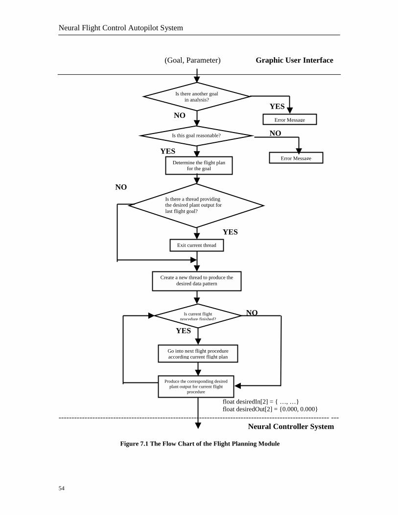
Neural Flight Control Autopilot System
54
(Goal, Parameter) Graphic User Interface
YES NO
NO
YES
NO
YES
YES
NO
YES
float desiredIn[2] = { …, …} float desiredOut[2] = {0.000, 0.000} -------------------------------------------------------------------------------------------------------- --- Neural Controller System
Figure 7.1 The Flow Chart of the Flight Planning Module
Error Message
Is this goal reasonable?
Is there another goal in analysis?
Error Message
Determine the flight plan for the goal
Is there a thread providing the desired plant output for last flight goal?
Is current flight procedure finished?
Go into next flight procedure according current flight plan
Produce the corresponding desired plant output for current flight
procedure
Exit current thread
Create a new thread to produce the desired data pattern
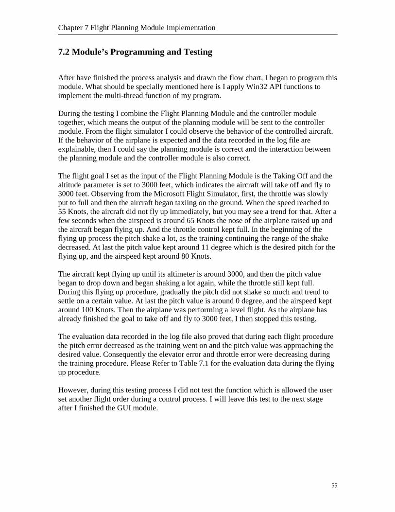
Chapter 7 Flight Planning Module Implementation
55
7.2 Module’s Programming and Testing After have finished the process analysis and drawn the flow chart, I began to program this module. What should be specially mentioned here is I apply Win32 API functions to implement the multi-thread function of my program. During the testing I combine the Flight Planning Module and the controller module together, which means the output of the planning module will be sent to the controller module. From the flight simulator I could observe the behavior of the controlled aircraft. If the behavior of the airplane is expected and the data recorded in the log file are explainable, then I could say the planning module is correct and the interaction between the planning module and the controller module is also correct. The flight goal I set as the input of the Flight Planning Module is the Taking Off and the altitude parameter is set to 3000 feet, which indicates the aircraft will take off and fly to 3000 feet. Observing from the Microsoft Flight Simulator, first, the throttle was slowly put to full and then the aircraft began taxiing on the ground. When the speed reached to 55 Knots, the aircraft did not fly up immediately, but you may see a trend for that. After a few seconds when the airspeed is around 65 Knots the nose of the airplane raised up and the aircraft began flying up. And the throttle control kept full. In the beginning of the flying up process the pitch shake a lot, as the training continuing the range of the shake decreased. At last the pitch value kept around 11 degree which is the desired pitch for the flying up, and the airspeed kept around 80 Knots. The aircraft kept flying up until its altimeter is around 3000, and then the pitch value began to drop down and began shaking a lot again, while the throttle still kept full. During this flying up procedure, gradually the pitch did not shake so much and trend to settle on a certain value. At last the pitch value is around 0 degree, and the airspeed kept around 100 Knots. Then the airplane was performing a level flight. As the airplane has already finished the goal to take off and fly to 3000 feet, I then stopped this testing. The evaluation data recorded in the log file also proved that during each flight procedure the pitch error decreased as the training went on and the pitch value was approaching the desired value. Consequently the elevator error and throttle error were decreasing during the training procedure. Please Refer to Table 7.1 for the evaluation data during the flying up procedure. However, during this testing process I did not test the function which is allowed the user set another flight order during a control process. I will leave this test to the next stage after I finished the GUI module.
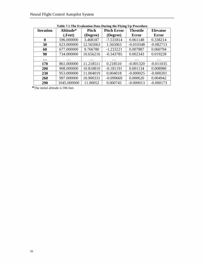
Neural Flight Control Autopilot System
56
Table 7.1 The Evaluation Data During the Flying Up Procedure Iteration Altitude*
(.Feet) Pitch
(Degree) Pitch Error
(Degree) Throttle
Error Elevator
Error 0 596.000000 3.468187 -7.531814 0.061148 0.338214 30 623.000000 12.565063 1.565063 -0.010348 -0.082713 60 677.000000 9.766780 -1.233221 0.007887 0.060794 90 734.000000 10.656216 -0.343785 0.002343 0.019228 … … … … … …
170 861.000000 11.218511 0.218510 -0.001320 -0.011035 200 908.000000 10.818810 -0.181191 0.001134 0.008980 230 953.000000 11.004019 0.004018 -0.000025 -0.000201 260 997.000000 10.900331 -0.099669 0.000620 0.004942 290 1045.000000 11.00052 0.000745 -0.000013 -0.000173
*The initial altitude is 596 feet.

Chapter 8 Graphic User Interface Module Implementation
57
Chapter 8 Graphic User Interface Module Implementation 8.1 Implementation Based on the design of the graphic user interface shown in section 4.2, I have written the programs with the help of Windows API functions. I applied Windows GDI (Graphic Device Interface) to implement the visualization function.
Figure 8.1 The Graphic User Interface
Figure 8.1 shows this graphic user interface and Figure 8.2 shows the sub-window which is used to visualize the evaluation data. This window will appear when the Graph button in the main window has been pressed.
Figure 8.2 The Graph Window
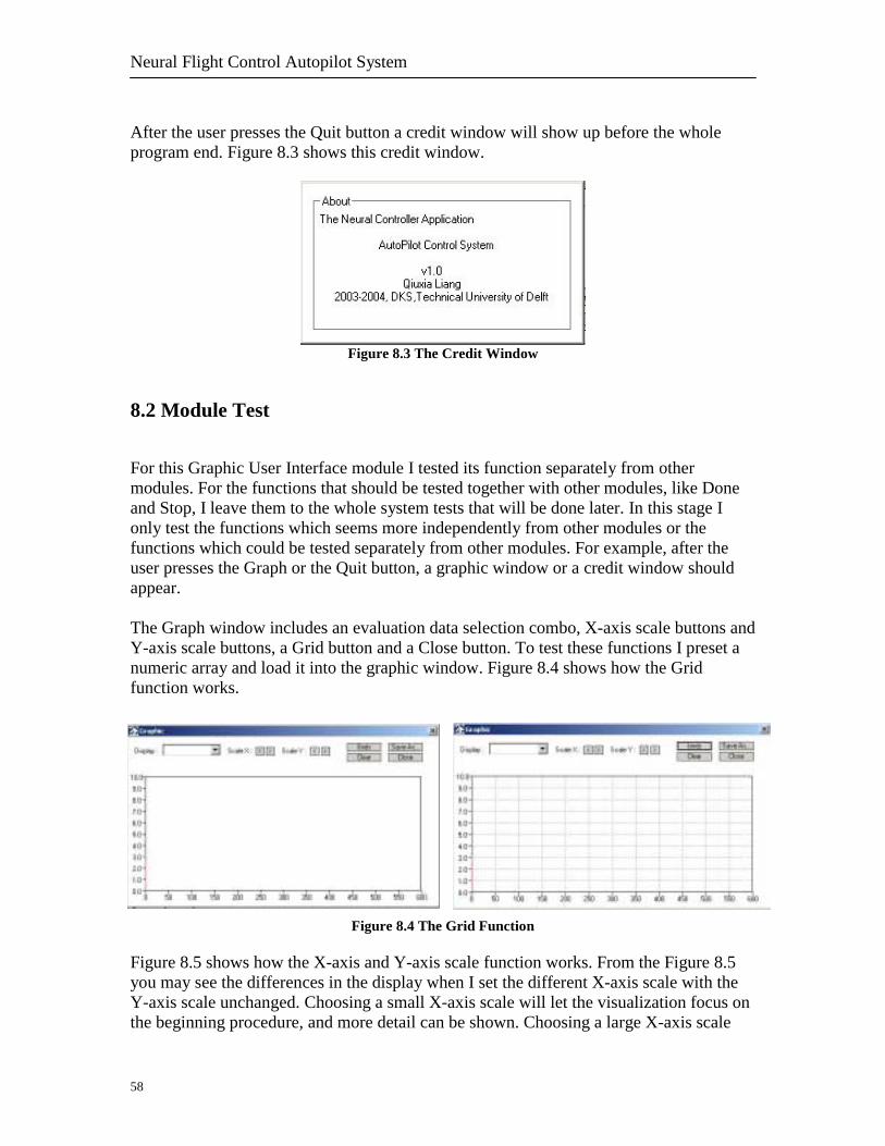
Neural Flight Control Autopilot System
58
After the user presses the Quit button a credit window will show up before the whole program end. Figure 8.3 shows this credit window.
Figure 8.3 The Credit Window
8.2 Module Test For this Graphic User Interface module I tested its function separately from other modules. For the functions that should be tested together with other modules, like Done and Stop, I leave them to the whole system tests that will be done later. In this stage I only test the functions which seems more independently from other modules or the functions which could be tested separately from other modules. For example, after the user presses the Graph or the Quit button, a graphic window or a credit window should appear. The Graph window includes an evaluation data selection combo, X-axis scale buttons and Y-axis scale buttons, a Grid button and a Close button. To test these functions I preset a numeric array and load it into the graphic window. Figure 8.4 shows how the Grid function works.
Figure 8.4 The Grid Function Figure 8.5 shows how the X-axis and Y-axis scale function works. From the Figure 8.5 you may see the differences in the display when I set the different X-axis scale with the Y-axis scale unchanged. Choosing a small X-axis scale will let the visualization focus on the beginning procedure, and more detail can be shown. Choosing a large X-axis scale
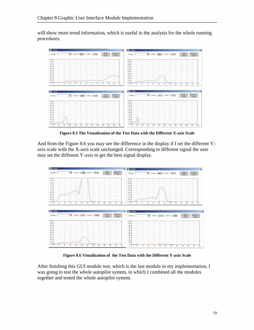
Chapter 8 Graphic User Interface Module Implementation
59
will show more trend information, which is useful in the analysis for the whole running procedures.
Figure 8.5 The Visualization of the Test Data with the Different X-axis Scale And from the Figure 8.6 you may see the difference in the display if I set the different Y-axis scale with the X-axis scale unchanged. Corresponding to different signal the user may set the different Y-axis to get the best signal display.
Figure 8.6 Visualization of the Test Data with the Different Y-axis Scale After finishing this GUI module test, which is the last module in my implementation, I was going to test the whole autopilot system, in which I combined all the modules together and tested the whole autopilot system.

60

61
Part III
Results, Conclusions and Recommendations

62
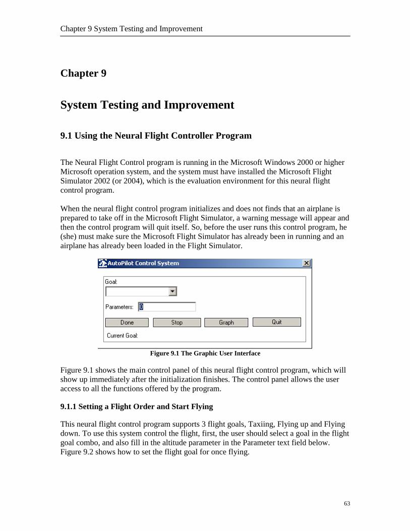
Chapter 9 System Testing and Improvement
63
Chapter 9 System Testing and Improvement 9.1 Using the Neural Flight Controller Program The Neural Flight Control program is running in the Microsoft Windows 2000 or higher Microsoft operation system, and the system must have installed the Microsoft Flight Simulator 2002 (or 2004), which is the evaluation environment for this neural flight control program. When the neural flight control program initializes and does not finds that an airplane is prepared to take off in the Microsoft Flight Simulator, a warning message will appear and then the control program will quit itself. So, before the user runs this control program, he (she) must make sure the Microsoft Flight Simulator has already been in running and an airplane has already been loaded in the Flight Simulator.
Figure 9.1 The Graphic User Interface
Figure 9.1 shows the main control panel of this neural flight control program, which will show up immediately after the initialization finishes. The control panel allows the user access to all the functions offered by the program. 9.1.1 Setting a Flight Order and Start Flying This neural flight control program supports 3 flight goals, Taxiing, Flying up and Flying down. To use this system control the flight, first, the user should select a goal in the flight goal combo, and also fill in the altitude parameter in the Parameter text field below. Figure 9.2 shows how to set the flight goal for once flying.
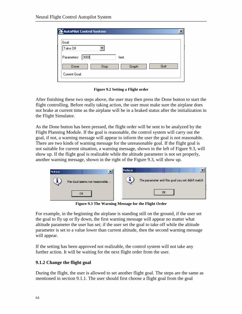
Neural Flight Control Autopilot System
64
Figure 9.2 Setting a Flight order
After finishing these two steps above, the user may then press the Done button to start the flight controlling. Before really taking action, the user must make sure the airplane does not brake at current time as the airplane will be in a braked status after the initialization in the Flight Simulator. As the Done button has been pressed, the flight order will be sent to be analyzed by the Flight Planning Module. If the goal is reasonable, the control system will carry out the goal, if not, a warning message will appear to inform the user the goal is not reasonable. There are two kinds of warning message for the unreasonable goal. If the flight goal is not suitable for current situation, a warning message, shown in the left of Figure 9.3, will show up. If the flight goal is realizable while the altitude parameter is not set properly, another warning message, shown in the right of the Figure 9.3, will show up.
Figure 9.3 The Warning Message for the Flight Order For example, in the beginning the airplane is standing still on the ground, if the user set the goal to fly up or fly down, the first warning message will appear no matter what altitude parameter the user has set; if the user set the goal to take off while the altitude parameter is set to a value lower than current altitude, then the second warning message will appear. If the setting has been approved not realizable, the control system will not take any further action. It will be waiting for the next flight order from the user. 9.1.2 Change the flight goal During the flight, the user is allowed to set another flight goal. The steps are the same as mentioned in section 9.1.1. The user should first choose a flight goal from the goal
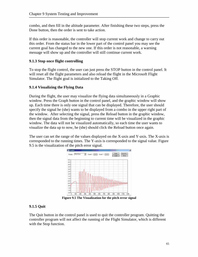
Chapter 9 System Testing and Improvement
65
combo, and then fill in the altitude parameter. After finishing these two steps, press the Done button, then the order is sent to take action. If this order is reasonable, the controller will stop current work and change to carry out this order. From the status bar in the lower part of the control panel you may see the current goal has changed to the new one. If this order is not reasonable, a warning message will show up and the controller will still continue current work. 9.1.3 Stop once flight controlling To stop the flight control, the user can just press the STOP button in the control panel. It will reset all the flight parameters and also reload the flight in the Microsoft Flight Simulator. The flight goal is initialized to the Taking Off. 9.1.4 Visualizing the Flying Data During the flight, the user may visualize the flying data simultaneously in a Graphic window. Press the Graph button in the control panel, and the graphic window will show up. Each time there is only one signal that can be displayed. Therefore, the user should specify the signal he (she) wants to be displayed from a combo in the upper right part of the window. After selecting the signal, press the Reload button in the graphic window, then the signal data from the beginning to current time will be visualized in the graphic window. The data will not be visualized automatically, so each time the user wants to visualize the data up to now, he (she) should click the Reload button once again. The user can set the range of the values displayed on the X-axis and Y-axis. The X-axis is corresponded to the running times. The Y-axis is corresponded to the signal value. Figure 9.5 is the visualization of the pitch error signal.
Figure 9.5 The Visualization for the pitch error signal 9.1.5 Quit The Quit button in the control panel is used to quit the controller program. Quitting the controller program will not affect the running of the Flight Simulator, which is different with the Stop function.

Neural Flight Control Autopilot System
66
Before the controller program quits, a credit window will appear. It will vanish after you click the left mouse button in it, and then the whole neural flight controller program will quit from the operation system. 9.2 System Testing During the implementation phase of each module, I have already tested their functions separately. Here I combine all the 3 modules together and test the functions of the whole neural flight control system. The objectives of the system testing include:
- Test the controlling function for each flight goal, make sure the controller system can work properly;
- Test the function that allows the user changing the flight goal during the flight controlling;
- Test the Stop function, make sure it can reset all the flight parameters and reload a flight in Flight Simulator to wait for a new control process;
- Test the Graph function, make sure it can be used to visualize the evaluation data in real-time and all functions under it work properly;
- Test the Quit function, make sure it is able to end this Neural Flight Control program and all the sub windows belonging to this program will quit together;
- Test and compare the output value from the identifier and the real output value from the airplane plant;
- Evaluate the stability of control; 9.2.1 Testing the Controlling Function For this testing, first, I set the flight goal to take off to 3000 feet. Observing from the Flight Simulation directly, in the taxiing process, as the throttle was put to full slowly the aircraft began taxiing on the ground. The status bar in the bottom of the control panel indicated current status was Taxiing, as shown in the left of Figure 9.6. When the speed reached to 55 Knots, the aircraft did not fly up immediately, however, you could see from the Flight Simulator, the airplane had the trend to leave the ground. After a few seconds when the airspeed was around 65 knots the pitch raised up and the aircraft began flying up.
Figure 9.6 The Control Panel with the Status Bar

Chapter 9 System Testing and Improvement
67
From the status bar in the main control panel you might see the airplane has already gone to the flying up status, as shown in the right of Figure 9.6. The throttle control still kept full. In the beginning of the flying up process the pitch shakes upward and downward a lot. As the training continued the range of the shake decreased. At last the pitch value kept around 11 degree which is the desired pitch for the flying up, and the airspeed kept around 70 knots. People can always refer to the flight instruments to get the airplane information during the flight. Figure 9.7 shows the 6 most important flight instruments. You can ignore the lower left two instruments because in this application the airplane only performs the straight flight. This figure was captured when the pitch settled on a certain degree during the flying up procedure.
Figure 9.7 The Flight Instruments at the final procedure of the Flying up The airspeed indicator shows that currently the airplane was flying at the speed of 70 Knots. The attitude indicator shows the pitch value of the airplane is around 12 degree, and the altimeter, which is located to the right of the attitude indicator, shows that the current altitude is around 2800 feet. The vertical speed indicator proved the airplane was flying up, and the vertical speed is around 600 Knots. 50 feet before the airplane reached the desired altitude, its flight behavior changed again. From the status bar I could see the flight was going into the default flying, which means the level flight. Similar to the procedure of going from taxiing to flying up, in the beginning of the default flying the airplane pitched a lot. As the flight (training) went on, the pitching magnitude decreased and the pitch value turned to keep on a certain value. Observed from the attitude indicator the pitch was exactly kept on 0 degree. However, from the altitude indicator the biggest hand (the hundred-foot hand) was moving counterclockwise, which means the altitude of the airplane was decreasing. The vertical speed indicator has proved this. Figure 9.8 shows what those instruments indicate at this moment of the default flying.
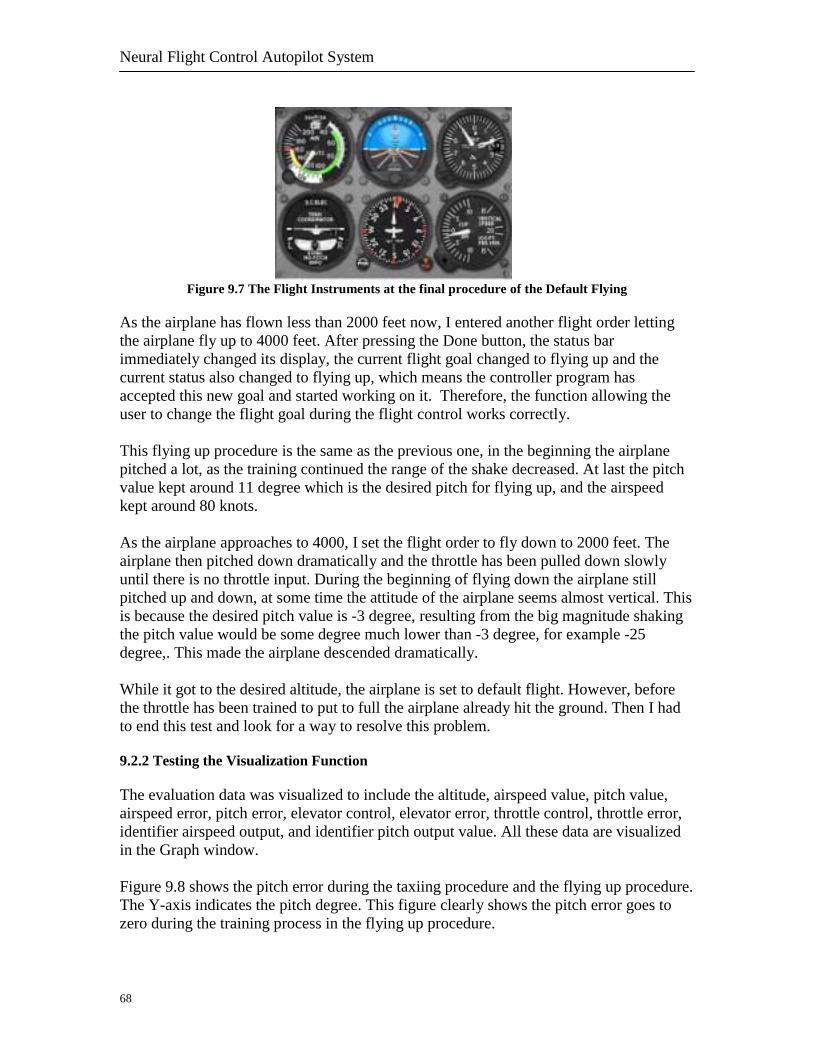
Neural Flight Control Autopilot System
68
Figure 9.7 The Flight Instruments at the final procedure of the Default Flying As the airplane has flown less than 2000 feet now, I entered another flight order letting the airplane fly up to 4000 feet. After pressing the Done button, the status bar immediately changed its display, the current flight goal changed to flying up and the current status also changed to flying up, which means the controller program has accepted this new goal and started working on it. Therefore, the function allowing the user to change the flight goal during the flight control works correctly. This flying up procedure is the same as the previous one, in the beginning the airplane pitched a lot, as the training continued the range of the shake decreased. At last the pitch value kept around 11 degree which is the desired pitch for flying up, and the airspeed kept around 80 knots. As the airplane approaches to 4000, I set the flight order to fly down to 2000 feet. The airplane then pitched down dramatically and the throttle has been pulled down slowly until there is no throttle input. During the beginning of flying down the airplane still pitched up and down, at some time the attitude of the airplane seems almost vertical. This is because the desired pitch value is -3 degree, resulting from the big magnitude shaking the pitch value would be some degree much lower than -3 degree, for example -25 degree,. This made the airplane descended dramatically. While it got to the desired altitude, the airplane is set to default flight. However, before the throttle has been trained to put to full the airplane already hit the ground. Then I had to end this test and look for a way to resolve this problem. 9.2.2 Testing the Visualization Function The evaluation data was visualized to include the altitude, airspeed value, pitch value, airspeed error, pitch error, elevator control, elevator error, throttle control, throttle error, identifier airspeed output, and identifier pitch output value. All these data are visualized in the Graph window. Figure 9.8 shows the pitch error during the taxiing procedure and the flying up procedure. The Y-axis indicates the pitch degree. This figure clearly shows the pitch error goes to zero during the training process in the flying up procedure.
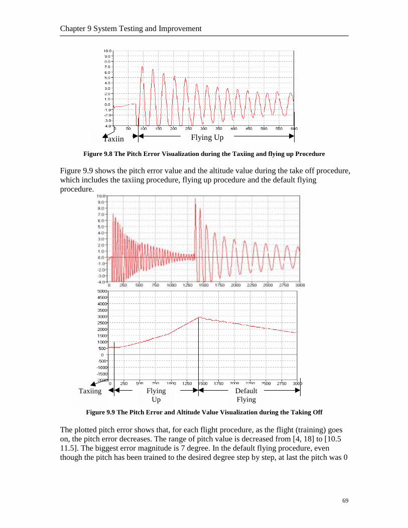
Chapter 9 System Testing and Improvement
69
Figure 9.8 The Pitch Error Visualization during the Taxiing and flying up Procedure
Figure 9.9 shows the pitch error value and the altitude value during the take off procedure, which includes the taxiing procedure, flying up procedure and the default flying procedure.
Figure 9.9 The Pitch Error and Altitude Value Visualization during the Taking Off
The plotted pitch error shows that, for each flight procedure, as the flight (training) goes on, the pitch error decreases. The range of pitch value is decreased from [4, 18] to [10.5 11.5]. The biggest error magnitude is 7 degree. In the default flying procedure, even though the pitch has been trained to the desired degree step by step, at last the pitch was 0
Default Flying
Flying Up
Taxiing
Flying Up Taxiin

Neural Flight Control Autopilot System
70
Degree, the airplane has kept descending all the time and in a fast way. During this flight the biggest pitch error magnitude is 8 degree.
Altitude Airspeed Airspeed Error
Elevator Input Elevator Error Pitch
Pitch Error Throttle Input Throttle Error
Figure 9.10 The visualization of the evaluation signals during the Taking Off and Flying Up
Besides of the pitch error signal and the altitude signal, I tested the visualization function for all the other signals also. Figure 9.10 shows the plots of those signals during the taking off to 3000 feet flight procedures. The testing helped me to make sure all the functions in the graph window, like the scaling function, Reload function, and etc, are working properly.
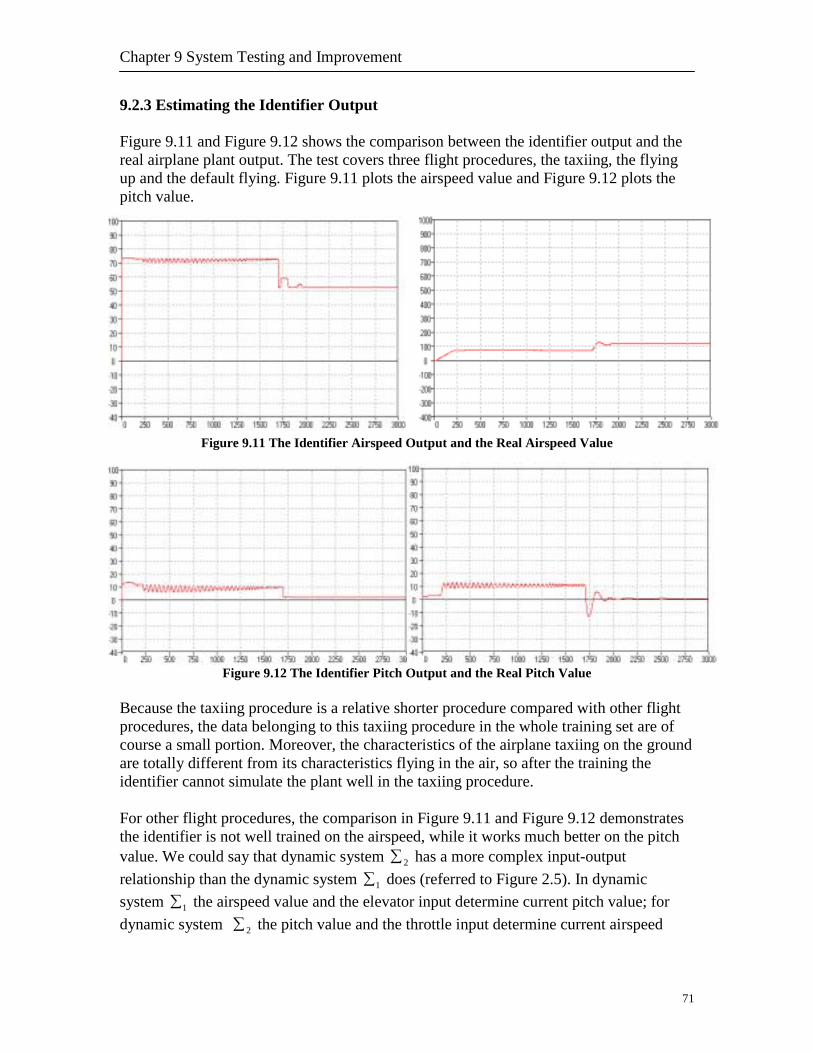
Chapter 9 System Testing and Improvement
71
9.2.3 Estimating the Identifier Output Figure 9.11 and Figure 9.12 shows the comparison between the identifier output and the real airplane plant output. The test covers three flight procedures, the taxiing, the flying up and the default flying. Figure 9.11 plots the airspeed value and Figure 9.12 plots the pitch value.
Figure 9.11 The Identifier Airspeed Output and the Real Airspeed Value
Figure 9.12 The Identifier Pitch Output and the Real Pitch Value Because the taxiing procedure is a relative shorter procedure compared with other flight procedures, the data belonging to this taxiing procedure in the whole training set are of course a small portion. Moreover, the characteristics of the airplane taxiing on the ground are totally different from its characteristics flying in the air, so after the training the identifier cannot simulate the plant well in the taxiing procedure. For other flight procedures, the comparison in Figure 9.11 and Figure 9.12 demonstrates the identifier is not well trained on the airspeed, while it works much better on the pitch value. We could say that dynamic system 2∑ has a more complex input-output relationship than the dynamic system 1∑ does (referred to Figure 2.5). In dynamic system 1∑ the airspeed value and the elevator input determine current pitch value; for dynamic system 2∑ the pitch value and the throttle input determine current airspeed

Neural Flight Control Autopilot System
72
value. With the same training data the airspeed variable requires more effort to be trained, compared with the pitch variable. The interesting thing is even though there is an inaccuracy in the identifier, the controller neural network has not been affected so much, and still been trained more and more better to control the flight. 9.2.4 Testing the Miscellaneous Functions Besides the testing above, I have also tested the Stop function and the Quit function to make sure they work correctly. Stop is used to stop the current flight procedure, reset all the parameters, and let the Flight Simulator reload the airplane to wait for another flight control. After pressing the Stop button, the flight goal in the control panel has been reset to Taking Off, there is no display in the status bar, and the Flight Simulator stops the current flying process and begins to reload a flight. After the airplane in the Flight Simulator has been loaded, I made the flight order from the control panel to test if the system really has been reset properly. The test results prove the Stop function works correctly. The testing on the Quit function, which is used to quit the whole controller program, also shows it is working correctly. 9.3 Improvements From the testing above, I should do some improvements on the current neural flight control system to solve the following problems,
- The dramatically shakings during in the beginning phase of each flight procedure; - From the flying down procedure going to the default flying procedure the
controller neural network has not enough time to get trained before it hits the ground;
- During the default flying procedure even the pitch has been trained to 0 Degree gradually, the airplane has kept descending all the time and in a fast way. See Figure 9.9;
- When the flight is going from the taxiing procedure to the flying up procedure, or from the flying up procedure to default flying procedure or to flying down procedure, the airplane pitches in a large degree.
Corresponding to these problems, my solutions are,
- Limit the controller’s output range, because the controller’s output is the input of the plant. The limiting on the elevator control value could consequently reduce the shaking range of the pitch;
- From one flight procedure going to another, the controller neural network always need some time to be trained properly. Since a general controller neural network cannot be trained, it is better use a different controller neural network for different
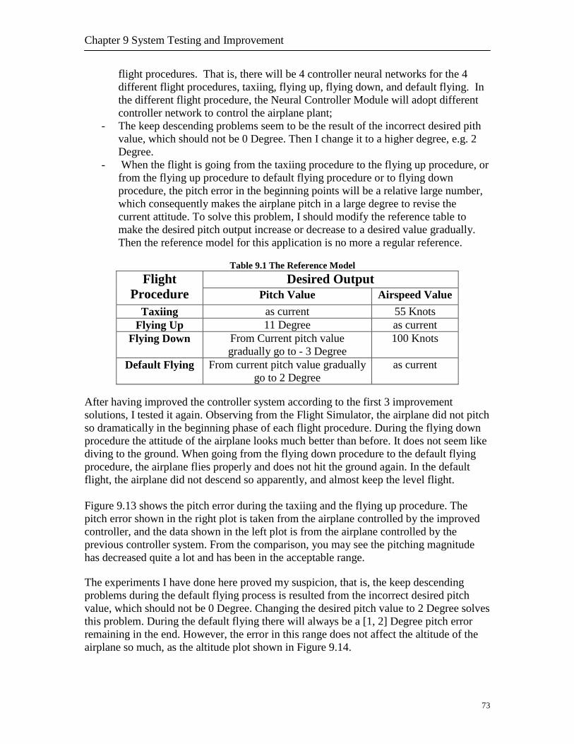
Chapter 9 System Testing and Improvement
73
flight procedures. That is, there will be 4 controller neural networks for the 4 different flight procedures, taxiing, flying up, flying down, and default flying. In the different flight procedure, the Neural Controller Module will adopt different controller network to control the airplane plant;
- The keep descending problems seem to be the result of the incorrect desired pith value, which should not be 0 Degree. Then I change it to a higher degree, e.g. 2 Degree.
- When the flight is going from the taxiing procedure to the flying up procedure, or from the flying up procedure to default flying procedure or to flying down procedure, the pitch error in the beginning points will be a relative large number, which consequently makes the airplane pitch in a large degree to revise the current attitude. To solve this problem, I should modify the reference table to make the desired pitch output increase or decrease to a desired value gradually. Then the reference model for this application is no more a regular reference.
Table 9.1 The Reference Model
Desired Output Flight Procedure Pitch Value Airspeed Value
Taxiing as current 55 Knots Flying Up 11 Degree as current
Flying Down From Current pitch value gradually go to - 3 Degree
100 Knots
Default Flying From current pitch value gradually go to 2 Degree
as current
After having improved the controller system according to the first 3 improvement solutions, I tested it again. Observing from the Flight Simulator, the airplane did not pitch so dramatically in the beginning phase of each flight procedure. During the flying down procedure the attitude of the airplane looks much better than before. It does not seem like diving to the ground. When going from the flying down procedure to the default flying procedure, the airplane flies properly and does not hit the ground again. In the default flight, the airplane did not descend so apparently, and almost keep the level flight. Figure 9.13 shows the pitch error during the taxiing and the flying up procedure. The pitch error shown in the right plot is taken from the airplane controlled by the improved controller, and the data shown in the left plot is from the airplane controlled by the previous controller system. From the comparison, you may see the pitching magnitude has decreased quite a lot and has been in the acceptable range. The experiments I have done here proved my suspicion, that is, the keep descending problems during the default flying process is resulted from the incorrect desired pitch value, which should not be 0 Degree. Changing the desired pitch value to 2 Degree solves this problem. During the default flying there will always be a [1, 2] Degree pitch error remaining in the end. However, the error in this range does not affect the altitude of the airplane so much, as the altitude plot shown in Figure 9.14.
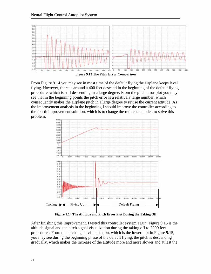
Neural Flight Control Autopilot System
74
Figure 9.13 The Pitch Error Comparison From Figure 9.14 you may see in most time of the default flying the airplane keeps level flying. However, there is around a 400 feet descend in the beginning of the default flying procedure, which is still descending in a large degree. From the pitch error plot you may see that in the beginning points the pitch error is a relatively large number, which consequently makes the airplane pitch in a large degree to revise the current attitude. As the improvement analysis in the beginning I should improve the controller according to the fourth improvement solution, which is to change the reference model, to solve this problem.
After finaltitude proceduyou maygraduall
g p
TaxiinFigure 9
ishing this imsignal and thres. From the see during ty, which mak
Flying U
.14 The Altitude and Pitch Err
provement, I tested this cone pitch signal visualization d pitch signal visualization, whe beginning phase of the dees the increase of the altitud
Default Flying
or Plot During the Taking Off
troller system again. Figure 9.15 is the uring the taking off to 2000 feet hich is the lower plot in Figure 9.15, fault flying, the pitch is descending e more and more slower and at last the
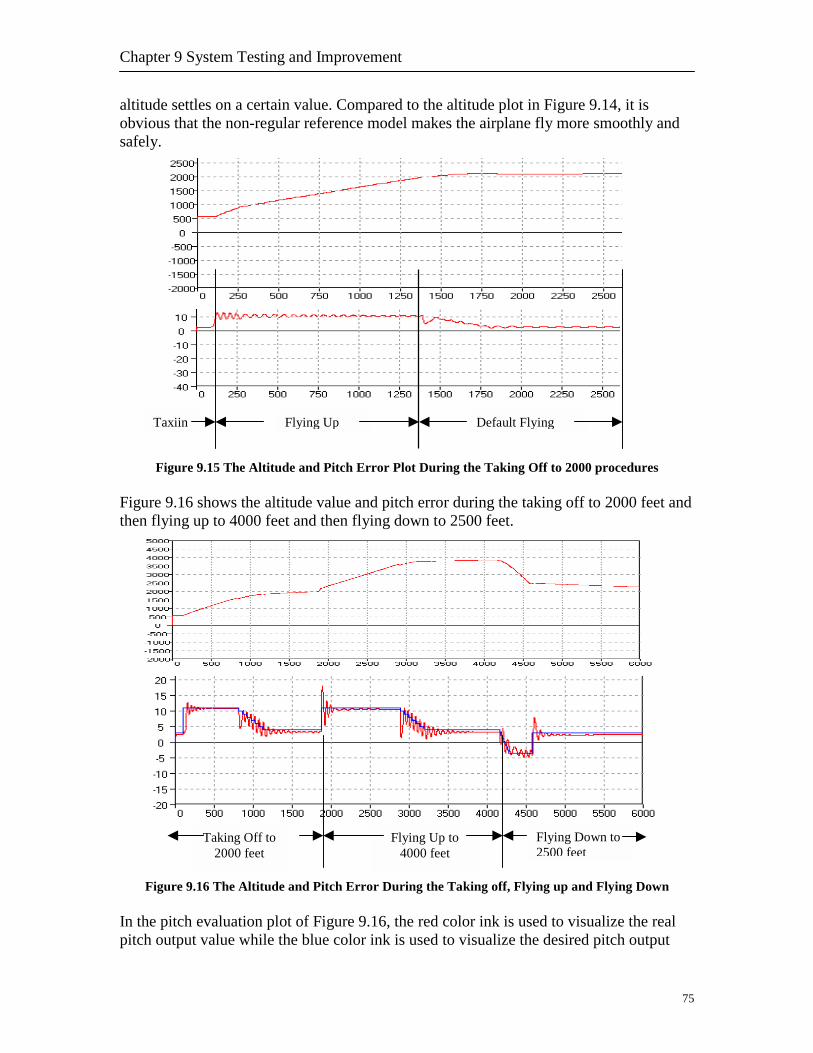
Chapter 9 System Testing and Improvement
altitude settles on a certain value. Compared to the altitude plot in Figure 9.14, it is obvious that the non-regular reference model makes the airplane fly more smoothly and safely.
Figure 9.15 The Altitude and Pitch Error Plot During the Taking Off to 2000 procedures
Figure 9.16 shows the altitude value and pitch error during the taking off to 2000 feet and then flying up to 4000 feet and then flying down to 2500 feet.
Figure 9.16 The Altitude and Pitch Error During the Taking off, Fly In the pitch evaluation plot of Figure 9.16, the red color ink is uspitch output value while the blue color ink is used to visualize th
Taking Off to 2000 feet
Flying Up to 4000 feet
Taxiin Flying Up Default Flying
Flying Down to 2500 feet
75
ing up and Flying Down
ed to visualize the real e desired pitch output

Neural Flight Control Autopilot System
76
value. From the comparison we can see that the neural controller can respond to the changes of the desired pitch value immediately. In another words, this neural controller has fast reaction ability. These testing results show the problems existing in the old controller system have been solved. Now the current neural flight controller system can achieve controlling the airplane to take off, fly up and flying down; the pitching magnitude during this flight procedures have been in an acceptable range; during flight the user can change the flight goal; the system provides the current flight situation to user and visualize the evaluation data in a 2D coordinators in real time. Therefore, all the required functions I defined for this controller system in the beginning have been achieved. 9.4 Controller Stability Analysis There are several ways to analyze the stability. For example, we may characterize stability from an input-output viewpoint, or we can characterize stability by studying the asymptotic behavior of the state of the system near steady-state solutions, like equilibrium points. Here I prefer to use the steady-state stability analysis. If this nonlinear aircraft system is represented by the state model,
)(xfx =& (9.1) where the x is a 2-dimensional vector, which include the parameters of the elevator control and the throttle control, defined in a domain nRD ⊂ . )(xf is locally Lipschitz functions of x . Suppose Dx ∈ is an equilibrium point of equation 9.1. Whenever the state of the system starts at x , it will remain at x for all future time. It is said to be asymptotically stable if it is stable and )(tx approaches to x as t tends to infinity. Starts with any element in a set of x , if the state approaches to x as t tends to infinity, then this set is called region of attraction (also called region of asymptotic stability, domain of attraction, or basin). When the region of attraction is the whole space nR , we define that the region is globally asymptotically stable. My goal is to study if the current system is asymptotic stable and characterize the attraction region.
Figure 9.17 The Elevator Input and the Throttle Input during the Flying Up Procedure
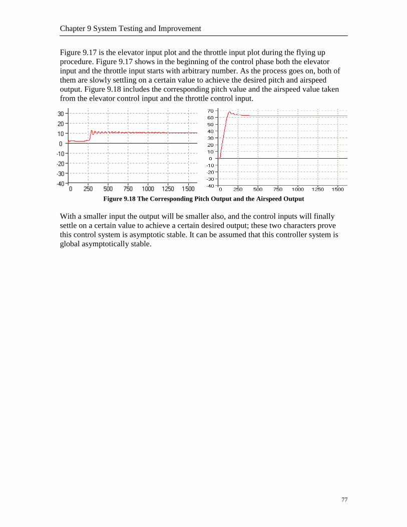
Chapter 9 System Testing and Improvement
77
Figure 9.17 is the elevator input plot and the throttle input plot during the flying up procedure. Figure 9.17 shows in the beginning of the control phase both the elevator input and the throttle input starts with arbitrary number. As the process goes on, both of them are slowly settling on a certain value to achieve the desired pitch and airspeed output. Figure 9.18 includes the corresponding pitch value and the airspeed value taken from the elevator control input and the throttle control input.
Figure 9.18 The Corresponding Pitch Output and the Airspeed Output With a smaller input the output will be smaller also, and the control inputs will finally settle on a certain value to achieve a certain desired output; these two characters prove this control system is asymptotic stable. It can be assumed that this controller system is global asymptotically stable.

78
Chapter 10 Conclusions and Discussions
79
Chapter 10 Conclusions and Discussions 10.1 Conclusions In this project I have developed a neural flight control system to control an airplane’s flight. The structure of the neural controller is called Feed Forward and Inverse Control, in which a pre-trained neural network is used to provide the error of the dynamic control, and an online learning neural network is used to compensate for the errors and then produce the control input. While the Neural Controller Module is producing the control data to the plant, a Flight Planning Module is working on the higher level to manage the global control in this autopilot system. The duties of the Flight Planning Module are producing the flight plans, building the corresponding reference model, and determining current flight situation. Except of these two modules there is another module, the Graphic User Interface Module, used to accept the flight order from the user, together with which they construct this neural flight control autopilot system. The results presented in the previous chapter demonstrate that the current neural flight controller system can - achieve controlling the airplane to take off, fly up and flying down; - run companied by the Microsoft Flight Simulator, which is a larger CPU time
consuming application; - control the airplane so that it achieves a stable flight; - has the ability to respond to the changes of the desired plant output immediately; - provide an graphic user interface to accept the order from the user, in which the user
could set flight order; - let the user set another flight order during flight; - provide the current flight situation to the user and visualize the evaluation data in 2D
coordinates in real time; The tests results also show that the training of the controller neural network is affected by the pre-defined desired plant output quite a lot. Therefore, setting the proper desired plant output for each flight procedure is very crucial for this neural flight controller system. During the improvement I have limited the output range of the elevator control to decrease the pitching magnitude, but the pitching phenomena still happens in the beginning phase of each flight procedure, which will directly cause the unsmooth flying. This pitching will disappear as the training goes on, though. Figure 10.4 shows the normalized elevator input, the pitch output during the flying up procedure, and the flying track of the airplane during this procedure.
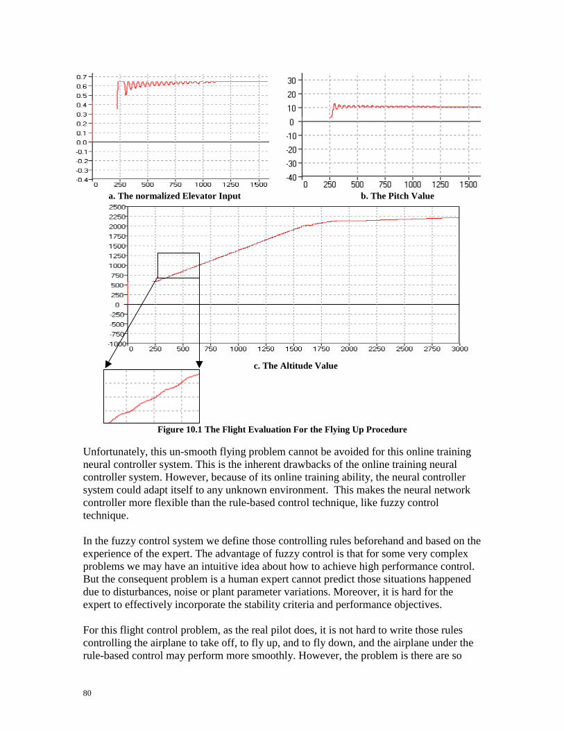
80
a. The normalized Elevator Input b. The Pitch Value
c. The Altitude Value
Figure 10.1 The Flight Evaluation For the Flying Up Procedure Unfortunately, this un-smooth flying problem cannot be avoided for this online training neural controller system. This is the inherent drawbacks of the online training neural controller system. However, because of its online training ability, the neural controller system could adapt itself to any unknown environment. This makes the neural network controller more flexible than the rule-based control technique, like fuzzy control technique. In the fuzzy control system we define those controlling rules beforehand and based on the experience of the expert. The advantage of fuzzy control is that for some very complex problems we may have an intuitive idea about how to achieve high performance control. But the consequent problem is a human expert cannot predict those situations happened due to disturbances, noise or plant parameter variations. Moreover, it is hard for the expert to effectively incorporate the stability criteria and performance objectives. For this flight control problem, as the real pilot does, it is not hard to write those rules controlling the airplane to take off, to fly up, and to fly down, and the airplane under the rule-based control may perform more smoothly. However, the problem is there are so
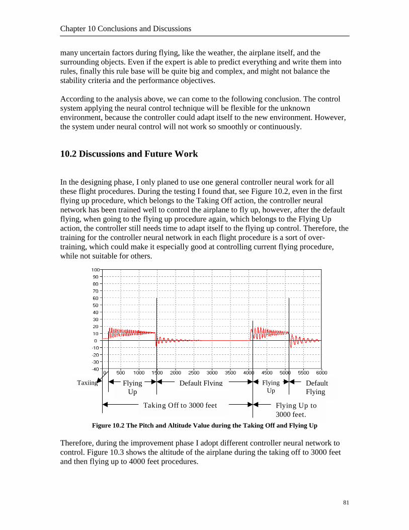
Chapter 10 Conclusions and Discussions
many uncertain factors during flying, like the weather, the airplane itself, and the surrounding objects. Even if the expert is able to predict everything and write them into rules, finally this rule base will be quite big and complex, and might not balance the stability criteria and the performance objectives. According to the analysis above, we can come to the following conclusion. The control system applying the neural control technique will be flexible for the unknown environment, because the controller could adapt itself to the new environment. However, the system under neural control will not work so smoothly or continuously. 10.2 Discussions and Future Work In the designing phase, I only planed to use one general controller neural work for all these flight procedures. During the testing I found that, see Figure 10.2, even in the first flying up procedure, which belongs to the Taking Off action, the controller neural network has been trained well to control the airplane to fly up, however, after the default flying, when going to the flying up procedure again, which belongs to the Flying Up action, the controller still needs time to adapt itself to the flying up control. Therefore, the training for the controller neural network in each flight procedure is a sort of over-training, which could make it especially good at controlling current flying procedure, while not suitable for others.
Thercontand
Flying g Flying g Default
TaxiinFigure 10.2 The Pitch and Alt
efore, during the improvement rol. Figure 10.3 shows the altituthen flying up to 4000 feet proc
Up
Taking Of
Default Flyin
81
itude Value during the Taking Off and Flying Up
phase I adopt different controller neural network to de of the airplane during the taking off to 3000 feet edures.
Up Flying
f to 3000 feet Flying Up to 3000 feet.

82
Figure 1 According to thand the Flying Uthe same controtrained well in tneeds time for t One reason couthe pitch equal faster the airspeon the elevator procedure and tdifferent from tbeen trained we
F As discussed insmoothly. Thouto constrain it. Tsolution is the fthere is a traininTherefore, not tcould be trained
Flying Up
Default Flyingp
Flying U0.3 The Altitude and Pitch Error Plot during the Taking Of
e pitch error data in the flying up procedures belongip respectively, you could see the problem has not b
ller neural network is applied to the Flying Up procehe Taking Off, when it is used again the controller nhe training.
ld be used to explain this situation. The proper elevato the desire value is depended on a current airspeed,ed, the more pressure the rear of airplane will have, control could get a larger change on the pitch value. he default flying procedure, the airspeed in the beginhe airspeed in the ending phase. That is why even if ll in the last time, when used again it still gets the tim
igure 10.4 How the Elevator Control Changes the airplane
the last section, the neural control system will makegh this un-smooth flying problem cannot be avoidedo make the airplane fly more smoothly under the ne
ollowing. For current neural network controller it geg pattern available, which will make the controller qraining the controller every time when one training p when, for example, 10 training patterns available. T
t
Default Flying
t
Taking Off to 3000 fee Flying up to 4000 feef and Flying Up
ng to the Taking Off een solved. Even if dure, after it has been eural network still
tor control to make see Figure 10.4, the so a smaller change For the flying up ning phase is the controller has
e to be trained well.
’s pitch
the airplane fly not , there are solutions ural controller, my ts trained at each time uite “sensitive”. attern is available, it hen the airplane
Chapter 10 Conclusions and Discussions
83
could keep the current pitch for a while, though the pitch will change after the next training, the airplane will seem to be flying more smoothly. For current neural flight control autopilot system, it only can control the airplane perform the straight flight. For future’s work, I hope to add more functions and take more things into account, e.g. the oil mixture rate, the weather information, the air transport information. The adding functions could make this neural flight control autopilot system
- control the airplane to make a turn; - control the airplane to land; - make the airplane fly more safely and smoothly.

84

Appendix
85
Appendix A. Aviation Introduction A.1 Flight Controls – Ailerons, Elevator, and Rudder Figure A.1 shows the three imaginary axes of the airplane. By use of the flight controls, the airplane can be made to rotate about one or more of these axes. [4]
Figure A.1 The Three Axes for an Airplane,
A – Vertical Axis (Yaw), B – Longitudinal Axis (Roll), C – Lateral Axis (Pitch)
The longitudinal axis runs through the centerline of the airplane from nose to tail. Airplanes roll about their longitudinal axis. The lateral axis runs sideways through the airplane from wingtip to wingtip. Airplanes pitch about their lateral axis. The vertical axis of the airplane runs up and down from the cockpit to the belly. Airplanes yaw about their vertical axis. Ailerons Ailerons are the moveable surfaces on the outer trailing edges of the wings. Their purpose is to bank the airplane in the direction you want to turn. When the control wheel is turned to the right, as shown in the left of Figure A.2, the ailerons simultaneously move in opposite directions. The left wing aileron lowers, increasing the lift on the left wing. The right wing aileron raises, decreasing the lift on the right wing. This causes the airplane to bank to the right. The right diagram in figure A.2 shows the situation when the control wheel is turned to the left.

Neural Flight Control Autopilot System
86
Figure A.2 Banking to the Right and Banking to the Left
Ailerons allow one wing to develop more lift and the other to develop less. Differential lift banks the airplane, which produces the total lifting force in the direction you want to turn. Elevator The elevator is the moveable horizontal surface at the rear of the airplane (Figure A.3). Its purpose is to pitch the airplane’s nose up or down.
Figure A.3 How the Elevator Control Changes the airplane’s pitch
The elevator control works on the same aerodynamic principle as the aileron. Applying back pressure on the control wheel of the airplane, as shown in the left of the Figure A.3, deflects the elevator surface upward.
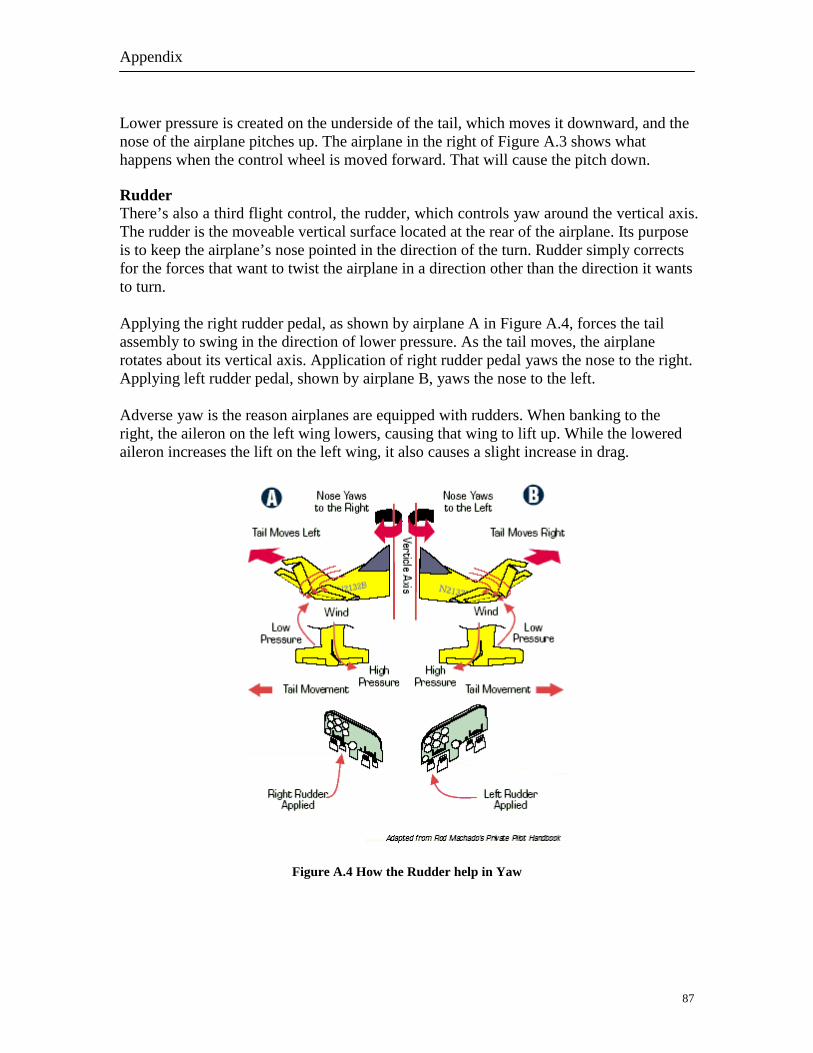
Appendix
87
Lower pressure is created on the underside of the tail, which moves it downward, and the nose of the airplane pitches up. The airplane in the right of Figure A.3 shows what happens when the control wheel is moved forward. That will cause the pitch down. Rudder There’s also a third flight control, the rudder, which controls yaw around the vertical axis. The rudder is the moveable vertical surface located at the rear of the airplane. Its purpose is to keep the airplane’s nose pointed in the direction of the turn. Rudder simply corrects for the forces that want to twist the airplane in a direction other than the direction it wants to turn. Applying the right rudder pedal, as shown by airplane A in Figure A.4, forces the tail assembly to swing in the direction of lower pressure. As the tail moves, the airplane rotates about its vertical axis. Application of right rudder pedal yaws the nose to the right. Applying left rudder pedal, shown by airplane B, yaws the nose to the left. Adverse yaw is the reason airplanes are equipped with rudders. When banking to the right, the aileron on the left wing lowers, causing that wing to lift up. While the lowered aileron increases the lift on the left wing, it also causes a slight increase in drag.
Figure A.4 How the Rudder help in Yaw
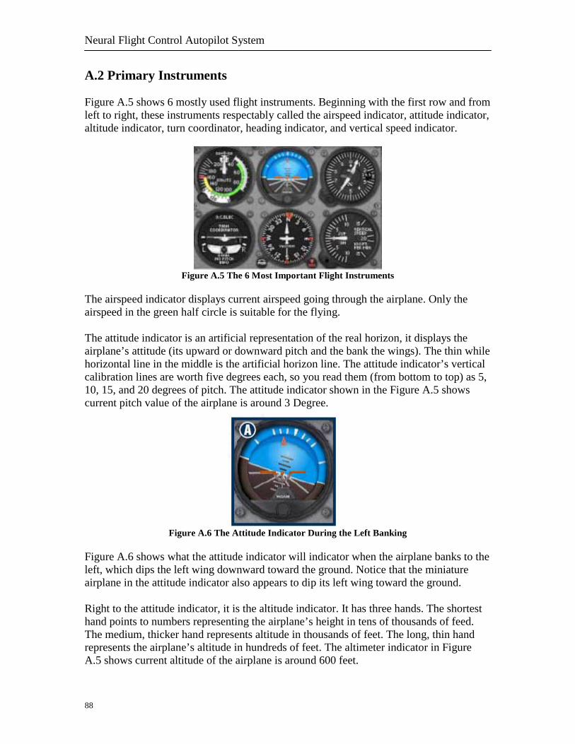
Neural Flight Control Autopilot System
88
A.2 Primary Instruments Figure A.5 shows 6 mostly used flight instruments. Beginning with the first row and from left to right, these instruments respectably called the airspeed indicator, attitude indicator, altitude indicator, turn coordinator, heading indicator, and vertical speed indicator.
Figure A.5 The 6 Most Important Flight Instruments The airspeed indicator displays current airspeed going through the airplane. Only the airspeed in the green half circle is suitable for the flying. The attitude indicator is an artificial representation of the real horizon, it displays the airplane’s attitude (its upward or downward pitch and the bank the wings). The thin while horizontal line in the middle is the artificial horizon line. The attitude indicator’s vertical calibration lines are worth five degrees each, so you read them (from bottom to top) as 5, 10, 15, and 20 degrees of pitch. The attitude indicator shown in the Figure A.5 shows current pitch value of the airplane is around 3 Degree.
Figure A.6 The Attitude Indicator During the Left Banking Figure A.6 shows what the attitude indicator will indicator when the airplane banks to the left, which dips the left wing downward toward the ground. Notice that the miniature airplane in the attitude indicator also appears to dip its left wing toward the ground. Right to the attitude indicator, it is the altitude indicator. It has three hands. The shortest hand points to numbers representing the airplane’s height in tens of thousands of feed. The medium, thicker hand represents altitude in thousands of feet. The long, thin hand represents the airplane’s altitude in hundreds of feet. The altimeter indicator in Figure A.5 shows current altitude of the airplane is around 600 feet.

Appendix
89
The heading indicator is a mechanical compass that shows which way the airplane points. Notice the numbers on the face of the heading indicator. Add a single zero to any number on the face to get the airplane’s actual heading. Directly below the altimeter is the vertical speed indicator (VSI). As its name suggests, its needle indicate the vertical speed of the airplane showing a rate of climb or descend.
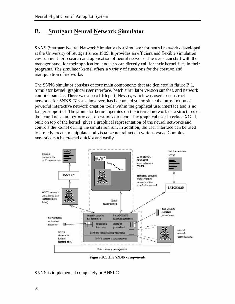
Neural Flight Control Autopilot System
90
B. Stuttgart Neural Network Simulator SNNS (Stuttgart Neural Network Simulator) is a simulator for neural networks developed at the University of Stuttgart since 1989. It provides an efficient and flexible simulation environment for research and application of neural network. The users can start with the manager panel for their application, and also can directly call for their kernel files in their programs. The simulator kernel offers a variety of functions for the creation and manipulation of networks. The SNNS simulator consists of four main components that are depicted in figure B.1, Simulator kernel, graphical user interface, batch simullator version snnsbat, and network compiler snns2c. There was also a fifth part, Nessus, which was used to construct networks for SNNS. Nessus, however, has become obsolete since the introduction of powerful interactive network creation tools within the graphical user interface and is no longer supported. The simulator kernel operates on the internal network data structures of the neural nets and performs all operations on them. The graphical user interface XGUI, built on top of the kernel, gives a graphical representation of the neural networks and controls the kernel during the simulation run. In addition, the user interface can be used to directly create, manipulate and visualize neural nets in various ways. Complex networks can be created quickly and easily.
Figure B.1 The SNNS components
SNNS is implemented completely in ANSI-C.
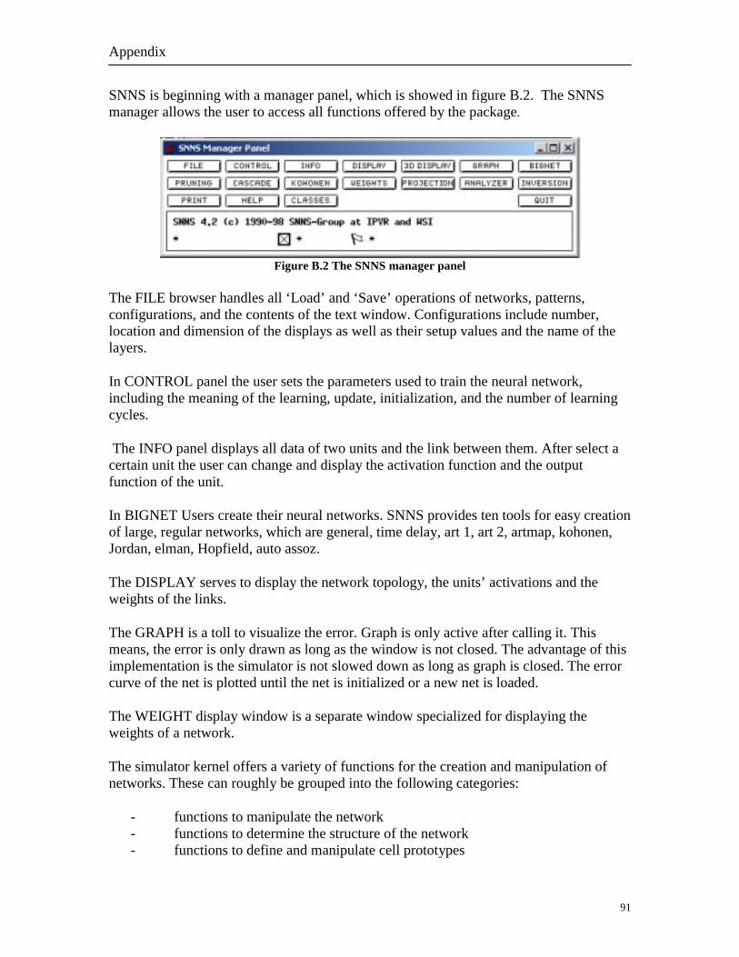
Appendix
91
SNNS is beginning with a manager panel, which is showed in figure B.2. The SNNS manager allows the user to access all functions offered by the package.
Figure B.2 The SNNS manager panel
The FILE browser handles all ‘Load’ and ‘Save’ operations of networks, patterns, configurations, and the contents of the text window. Configurations include number, location and dimension of the displays as well as their setup values and the name of the layers.
In CONTROL panel the user sets the parameters used to train the neural network, including the meaning of the learning, update, initialization, and the number of learning cycles.
The INFO panel displays all data of two units and the link between them. After select a certain unit the user can change and display the activation function and the output function of the unit.
In BIGNET Users create their neural networks. SNNS provides ten tools for easy creation of large, regular networks, which are general, time delay, art 1, art 2, artmap, kohonen, Jordan, elman, Hopfield, auto assoz.
The DISPLAY serves to display the network topology, the units’ activations and the weights of the links.
The GRAPH is a toll to visualize the error. Graph is only active after calling it. This means, the error is only drawn as long as the window is not closed. The advantage of this implementation is the simulator is not slowed down as long as graph is closed. The error curve of the net is plotted until the net is initialized or a new net is loaded.
The WEIGHT display window is a separate window specialized for displaying the weights of a network.
The simulator kernel offers a variety of functions for the creation and manipulation of networks. These can roughly be grouped into the following categories:
- functions to manipulate the network - functions to determine the structure of the network - functions to define and manipulate cell prototypes
Neural Flight Control Autopilot System
92
- functions to propagate the network - learning functions - functions to manipulate patterns - functions to load and save the network and pattern files - functions for error treatment, search functions for names, functions to change
default values etc.
In programming SNNS has its own way to represent the unit, the network, and the pattern. For more details about SNNS, you may refer to their home page,
http://www-ra.informatik.uni-tuebingen.de/SNNS/.
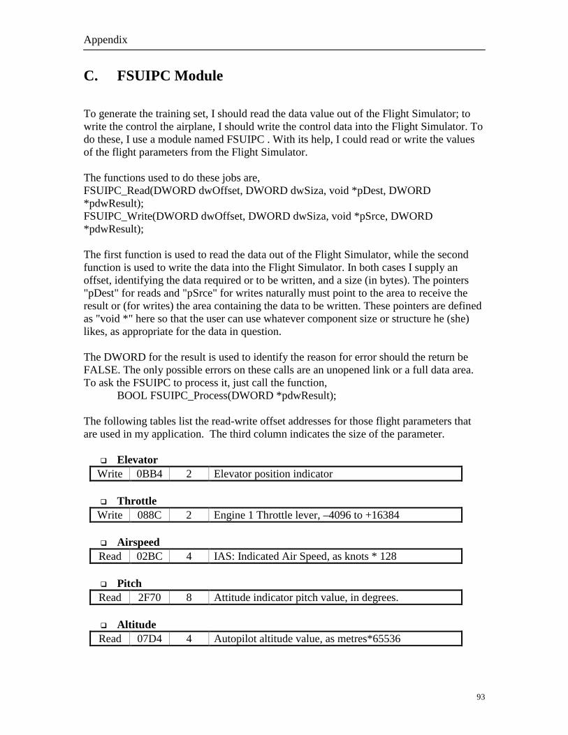
Appendix
93
C. FSUIPC Module To generate the training set, I should read the data value out of the Flight Simulator; to write the control the airplane, I should write the control data into the Flight Simulator. To do these, I use a module named FSUIPC . With its help, I could read or write the values of the flight parameters from the Flight Simulator. The functions used to do these jobs are, FSUIPC_Read(DWORD dwOffset, DWORD dwSiza, void *pDest, DWORD *pdwResult); FSUIPC_Write(DWORD dwOffset, DWORD dwSiza, void *pSrce, DWORD *pdwResult); The first function is used to read the data out of the Flight Simulator, while the second function is used to write the data into the Flight Simulator. In both cases I supply an offset, identifying the data required or to be written, and a size (in bytes). The pointers "pDest" for reads and "pSrce" for writes naturally must point to the area to receive the result or (for writes) the area containing the data to be written. These pointers are defined as "void *" here so that the user can use whatever component size or structure he (she) likes, as appropriate for the data in question. The DWORD for the result is used to identify the reason for error should the return be FALSE. The only possible errors on these calls are an unopened link or a full data area. To ask the FSUIPC to process it, just call the function, BOOL FSUIPC_Process(DWORD *pdwResult); The following tables list the read-write offset addresses for those flight parameters that are used in my application. The third column indicates the size of the parameter.
! Elevator Write 0BB4 2 Elevator position indicator
! Throttle
Write 088C 2 Engine 1 Throttle lever, –4096 to +16384
! Airspeed Read 02BC 4 IAS: Indicated Air Speed, as knots * 128
! Pitch Read 2F70 8 Attitude indicator pitch value, in degrees.
! Altitude Read 07D4 4 Autopilot altitude value, as metres*65536

Neural Flight Control Autopilot System
94
D. Neural Controller Module Implementation Details The following shows those sub-functions I used for each step to construct the Feed Forward and Inverse Controller, Step 1, to propagate a desired output pattern through the neural controller - krui_loadNet(char *filename, char **netname); load the net file
- krui_loadNewPatterns(char *filename, int *set_no); load the pattern file, optional, only for the first time loading the desired value patterns
- krui_setPatternNo(int pattern_no) ; sets the current pattern - krui_showPattern(int mode) ; according to the mode, krui_showPattern stores
the current Pattern into the units activation (or output) values. - krui_setUpdateFunc(char *update_func) ; changes the current update function,
because the default one is set to “Serial Order” , while in this application I need “Topological_Order”
- krui_updateNet(float *parameterInArray, int NoOfInParams); Updates the network according to update function
Step 2, to get the control data out of the corresponding neural controller for that desired value pattern - krui_getUnitOutput(int UnitNo) ; Returns the output value of the unit Step 3, to propagate the control data pattern through the neural identifier - krui_loadNet(char *filename, char **netname); load the net file
- krui_loadNewPatterns(char *filename, int *set_no); load the pattern file, optional, only for the first time loading the desired value patterns
- krui_setPatternNo(int pattern_no) ; sets the current pattern - krui_showPattern(int mode) ; according to the mode, krui_showPattern stores
the current Pattern into the units activation (or output) values. - krui_setUpdateFunc(char *update_func) ; changes the current update function,
because the default one is set to “Serial Order” , while in this application I need “Topological_Order”
- krui_updateNet(float *parameterInArray, int NoOfInParams); Updates the network according to update function
Step 4, to send the control data to the plant
- FSUIPC_Write(DWORD dwOffset, DWORD dwSize, void *pSrce, DWORD *pdwResult); Prepare the parameters used to write data to MS FS
- FSUIPC_Process(DWORD *pdwResult); Process the action Step 5, to read out the real output information from the plant
- FSUIPC_Read(DWORD dwOffset, DWORD dwSize, void *pDest, DWORD *pdwResult) ; Prepare the parameters used to write data to MS FS
- FSUIPC_Process(DWORD *pdwResult) ; Process the action Step 6, to get the error between the real output values and the desired values

Appendix
95
- The error is equal to the desired plant output value minus the real plant output value
Step 7and 8, to backpropage the error through neural identifier, and then get the corresponding error at the input layer
- float * Error_Backprop(int pattern_no, float learn_parameter, float delta_max); Calculate the Backpropagation Error for the Input units
Step 9, to train the neural controller assuming that the correct output is equal to the controller network output plusing the backpropagation error from the identifier - krui_setLearnFunc(char *learning_func); hangs the current learning function - krui_DefTrainSubPat(int *insize, int *outsize, int *instep, int *outstep, int *max_n_pos); define how sub patterns should be generated during training - krui_learnSinglePattern(int pattern_no, float *parameterInArray,
int NoOfInParams, float **parameterOutArray, int *NoOfOutParams); learns only based on the current pattern pair

96
References
97
References [1] G.W.Ng, 1997, Application of Neural Networks to Adaptive Control of Nonlinear System, Research Studies Press LTD. [2] K.J.Hunt and D.Sbarboro, 1995, Studies in artifical neural network based control, IEE Control Engineering Series. Vol. 53, PP 109-139
[3] J.C. Principe, N.R. Euliano and W.C. Lefebvre , 2000, Neural and Adaptive Systems: Fundamentals through Simulations, John Wiley & Sons, Inc. [4] R. Machado, Rod Machado’s Ground School, Available from the help documents in Microsoft Flight Simulator [5] J. Jarmulak, 1994, Neuro Control Workbench, MSc Thesis, Delft University of Technology [6] M.I. Jordan and D.E. Rumelhart, 1992, Forward models: Supervised learning with a distal teacher, Cognitive Science 16, no.3: 307-354 [7] Cleared for Takeoff, 1998, King Scholls, Available from King Schools or Cessna Pilot Centers. [8] P.A.M. Ehlert and L.J.M. Rothkrantz, 2003, The Intelligent Cockpit Environment Project, Research Report DKS03-04 / ICE 04, Delft University of Technology [9] H. Demircioglu and P.J. Gawthrop, 1991, Continuous-time generalized predictive control. Automatica 27, no. 1: 55-74
Neural Flight Control Autopilot System
98
[10] E. Hernandez and Y. Arkun, 1993, Control of nonlinear systems using polynomial ARMA models. AICHE Jouranl 39: 446-460 [11] S. Chen, S.A. Billings, C.F. Cowan and P.m. Grant, 1990, Practical identification of NARMAX models using radial basis functions. International Journal of Control 53: 1327-1350 [12] J. Kaneshige, J, Bull and J.J. Totah, 2000, Generic Neural Flight Control and Autopilot System, Available from http://ic.arc.nasa.gov/publications/pdf/2000-0172.pdf [13] I. Mareels and J. W. Polderman, 1996, Adaptive system: an introduction, Birkhauser Boston [14] D. Soloway and P.J.Haley, 1996, Neural Generalized Predictive Control, Proceedings of the 1996 IEEE International Symposium on Intelligent Control, PP 277-282 [15] P.J. Werbos, 1990, Backpropagation through time: What it does and how to do it? Proceedings of IEEE 78: 1550-1560