network planning - telenor group – telenor group is ... · pdf filenetwork planning 1...
TRANSCRIPT

Network Planning
1 Guest Editorial Terje Jensen
3 A Tale of a Technical Officer’s DayTerje Jensen
9 Network Planning – Introductory IssuesTerje Jensen
47 Optimization-Based Network Planning Tools in Telenor During the Last 15 Years – A SurveyRalph Lorentzen
68 Network Strategy StudiesTerje Jensen
99 Portfolio Evaluation Under UncertaintyRalph Lorentzen
110 Forecasting – An Important Factor for Network PlanningKjell Stordahl
122 Traffic Forecasting Models for the Incumbent Based on New Drivers in the MarketKjell Stordahl
128 Planning Dependable Network for IP/MPLS Over OpticsTerje Jensen
163 Terms and Acronyms – Network Planning
177 Telektronikk Index 2001 – 2003
Contents
Telektronikk
Volume 99 No. 3/4 – 2003
ISSN 0085-7130
Editors:
Ola Espvik
Tel: (+47) 913 14 507
Per Hjalmar Lehne
Tel: (+47) 916 94 909
Editorial assistant:
Gunhild Luke
Tel: (+47) 415 14 125
Editorial office:
Telenor ASA
Telenor R&D
NO-1331 Fornebu
Norway
Tel: (+47) 810 77 000
www.telenor.com/rd/telektronikk
Editorial board:
Berit Svendsen, CTO Telenor
Ole P. Håkonsen, Professor
Oddvar Hesjedal, Director
Bjørn Løken, Director
Graphic design:
Design Consult AS (Odd Andersen), Oslo
Layout and illustrations:
Gunhild Luke and Åse Aardal,
Telenor R&D
Prepress and printing:
Gan Optimal as, Oslo
Circulation:
3,100
1
Chance favours a prepared mind!– reflect on it ...
Spending some effort on systemising one’s situ-ation allows for a revelation of one’s strengthsand weaknesses. Moreover, it leads to steps totake in order to gain from “chances” by effi-ciently incorporating means into one’s portfolio.Spotting opportunities and smoothly turningthese into profitable operations is a key issue forany actor. As the market matures and the safe/traditional services and systems are deployed,new products and systems are required to main-tain more profitable operation. In particular asthe number of competing actors grows it isimportant not to lose out on the chances that turnup. Not every chance is to be seized though;only the ones that are expected to strengthenone’s situation.
So how can network planning assist? First, inorder to carry out the planning the actual situa-tion must be characterised, hence describing theoverall situation to the operator. This also out-lines strengths and weaknesses. Second, strate-gic planning commonly applies scenario workthat captures the possible future an operator mayexperience. The scenarios are characterised bya number of factors attached with uncertainties.These factors should therefore be particularlymonitored as time evolves. Third, relating poten-tial target states with the current situation revealsa roadmap describing specific events that mayhappen. These events may well reflect pointswhere decisions are to be made. Naturally, sev-eral factors have to be evaluated when preparingfor the decision, and these are also part of thenetwork planning. Fourth, simply discussing andelaborating the plans is likely to reveal furtheropportunities. That is, gathering a number ofindividuals from different departments helps toform several profitable ideas.
The ultimate outcome of a planning exercise isquantified numbers related to specific networksolutions. However, a mixture of qualitative andquantitative evaluations is included in the full-blown planning. One example of a fruitful mix-ture is to apply qualitative approaches for thewide set of options that might appear, while amore limited set is selected for the calculationexercise. The cases will also be taken intoaccount when conducting a number of what-ifevaluations. This also leads to the fundamental
role of network planning as a basis for manage-ment decision support.
Network planning has a range of scopes, asdescribed later in this issue. Several types ofinput and aspects have to be considered. In sepa-rating the time frames it is important that strate-gic, tactical and operational means are har-monised, which implies a need for good coordi-nation between the commonly different groupsmanaging the different scopes. A consequenceof this is that the strategic plans have to be con-nected to current operations in order to showeffects. This is one example that actions result-ing from planning would be organised along atime axis and be reflected in the organisation.
Considering the operator’s set of interdependentsystems, products, traffic flows and customers, itis essential to have a methodical support of theplanning exercises. Covering all combinations ofoptions, the tasks frequently become too tediousfor mere manual analyses. This also assists inassessing consequences and selecting betteractions for urgent questions, like responding tocompetitors’ product rollouts, sudden trafficincreases, offers from vendors, and so forth.
More than 125 years after Alexander GrahamBell’s invention in 1876, few people oppose thenotion that the electronic communication meansis one of the major indicators of a community’swelfare. This shows the essence of having ade-quately operational telecommunication networksand corresponding systems in a nation. Thenumber of people who are aware of the opportu-nities and are able to put the practical solutionsinto operation grows in importance as more can-didate solutions and arrangements are faced andcompetition levels fluctuate. Hence, the speedytechnological, market and service changes makeit more challenging for a network planner tokeep ahead of efficient network solutions. Theconvergence of telecommunications, informationsystems, broadcasting, user devices – partiallyfuelled by transition from complexity in hard-ware to software – requires that the networkplanning methodology is flexible and able toconsider the holistic view and take into accountfuture optional migration tracks.
The drivers for network planning include tech-nology, markets, business and customer service.It is the financial turmoil in the telecom industrythat has produced the latest changes. There is a
Guest EditorialT E R J E J E N S E N
Terje Jensen
Telektronikk 3/4.2003
Front cover:Network Planning
The overall basis for implementinga network plan is a global techno-economical optimal network solu-tion created through an optimisa-tion process. Such a global pro-cess involves a number of localdisciplines and problems.
The artist Odd Andersen visu-alises the iterative optimisationprocess as a spiral reaching in-wards to a desired target. In thesame manner the local processeshave to find their optimal solutionsgiven global constraints. The localprocesses are visualised as minorspirals interacting with – andadjusting the path of the globalprocess. This myriad of adjust-ments goes on until an acceptableglobal optimum is achieved. Toillustrate the new plans’ depen-dency on logical and physical net-work structures already present,Odd Andersen locates the optimi-sation process on top of the exist-ing band of possibilities.
Ola Espvik, Editor in Chief

2 Telektronikk 3/4.2003
renewed interest in cost reduction and maximis-ing use of resources which increases the need fornetwork planning. However, this also comes at atime of great technological change with IP-basedarchitectures and wireless access producing agreat potential for new applications, and there-fore additional planning challenges to be solved– and there is no sign that the pace of change isslowing.
The network planning area is too wide to be cov-ered by a single issue. However, a number ofaspects are treated in the following articles. Thefirst article provides a survey of network plan-ning, relating network planning to management/financial topics and the technical questions to betreated. Going directly to the core of the plan-ning task a survey of between one and twodecades of implementing planning tools isdescribed in the subsequent article.
The next area considered places more weight onthe strategic perspective. This is described by asurvey article as well as a more in-depth descrip-tion of risk considerations. Gone are the dayswith “never-failure” as the sole objective withless focus on delivery time-scales and solutioncost. Risk management is now a key as technicaland commercial risks are balanced against theneed to meet market opportunities on time and inaccordance with budget.
The essentials of markets must be understood asit profoundly affects network planning objec-tives. This is also documented in articles onforecasting, describing methodologies andresults for obtaining estimates of number ofcustomers and amount of traffic.
The final article returns to one of the centralquestions for backbone networks; that is, how toefficiently utilise the capacity of transport net-works.
As stated above, a full coverage is beyond thescope of any single issue. The main objective ofthis issue is to provide insight into systematicsand methodology applied for network planning.This also points to the need for awarenessregarding adequate planning competence, defin-ing relevant planning tasks and continuingassessment of input data and surveying the criti-cal events revealed through the planning work.The wider scope of planning is taken on describ-ing the need for on-going activities and linksbetween different planning tasks. In particular,linkage between long and short term planning, aswell as relations between different systems mustbe obeyed.
In order to provide the material in this issue ofTelektronikk, interesting discussions with a widerange of individuals have been appreciated. Theinterest for the questions addressed during pro-jects in later years clearly shows that networkplanning activities engage most people involvedin electronic communications.
Enjoy your reading!
3
IntroductionBleep – bleep, a message arrives on TO’smobile. The market survey group has spotted acompetitor launching a new product. Immediatequestion: “How do we respond to that?” Well,our technical officer, we will call him TO forshort, receives the news in a relaxed manner.Having gone through a set of possible scenarios,the one emerging has already been examined.And it turned out that the launched product doesnot allow sufficient profit margins compared tothe ones already offered. All calculation results,internal as well as jointly with others, showedthat this product will disappear from the marketagain – or the competitor will experienceincreasing loss. So a quick messaging reply wasissued: “Don’t worry – stay happy – and have alook at the strategy document on scenarios point6.4.” “Well, being prepared is rarely a disad-vantage,” TO thinks as he continues his break-fast. Soon he receives a reply, “Thanks – corre-sponding media action is under preparation”.“Well, a nice start to a sunny day,” TO thinks,pouring another glass of milk.
On the way to his office, TO happened to ob-serve the cars changing lanes without signalling,causing sudden breaking and changing speeds.Like most systems involving humans or uncoor-dinated instances – efficiency measured on theindividual level differs from that measured onthe overall system level. In this case a singledriver might believe that he is reaching his desti-nation very fast, while the total effect on all theother cars on the same road may be that they areall delayed. This could well be applied to tele-com systems. In fact, the inherent stochasticnature of systems, user behaviour and technicalcapabilities, competitors, governmental bodies,etc. further adds to the complexity of findingwhich steps to take to achieve company goals.Commonly these days, such goals are given asmaximising growth profit. In a telecom system,
however, traffic can mostly be directed morefreely than what is accepted on the road.
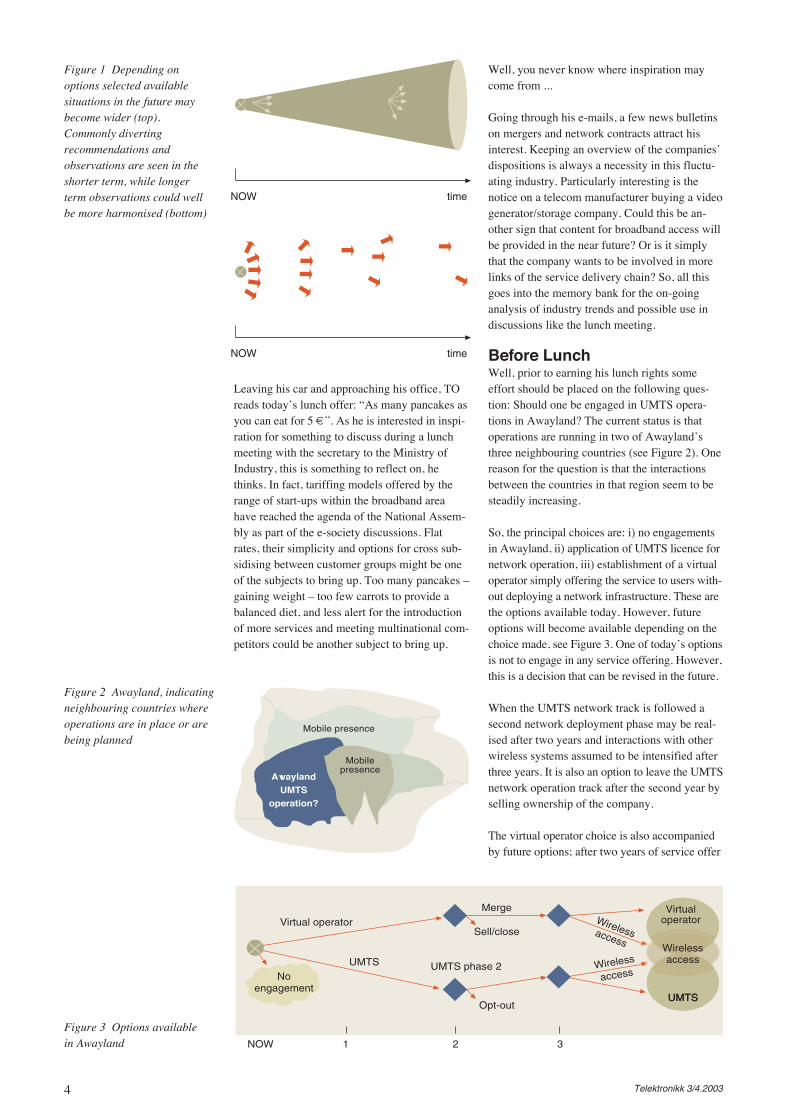
Approaching this in a systematic manner, thequestions can be arranged along a time axis. Thenthe number of options will likely grow with time.One pictorial model for this is to think of thefuture options as constructing a cone – a widerset of outcomes and actions are available in thelonger time horizon (see Figure 1). On the otherhand, one may also have a clearer picture of themajor trends dominating the picture. Hence, byshifting the scope in the longer term, the choicesto be made may be clearer on a general levelwhen considering the technical areas. Besides,several other areas have to be taken into accounteven though technical decisions have to be made.Such areas include financial means, customerrequests, competitors, regulatory issues, etc.Factors from these areas may well inspire addi-tional actions relating to technological choices.
Still, although there are a lot of uncertainties anumber of decisions have to be made. In order toensure a robust company portfolio, several strat-egies could be pursued, although this must be aclear company choice and not simply somethingthat happens because of lack of coordination.“Hm, this is almost on a philosophical level,”TO reflects.
Before Morning CoffeeParking his car around 07.30 our technical offi-cer TO notices that the car parking places areabout to be re-arranged into a common pool. Sofar, department-specific places have been allo-cated. To TO, with his planning background, thisseems like a natural step to take to increase theefficiency of the parking area; yet an example ofthe scale effect – loosely described as “the big-ger the better”. Again, some similarities betweencontrolling vehicular traffic and telecom trafficcould be recognised.
A Tale of a Technical Officer’s DayT E R J E J E N S E N
Imagine being a technical officer – or maybe you are? A long list of questions are raised about how to
get the highest return by smart spending of the company’s money. In a broader perspective everyone
involved in network evolution is faced with similar questions; how to organise the systems and system
management and how to allocate resources to achieve company goals. An intuitive statement, however,
is that the choices made have more dramatic effects when made at a higher level in the company. On
the other hand, every function must work in a coherent way to allow for flexible, rapid and efficent
service provisioning.
The following imaginary story tells about a workday of a technical officer, called TO. So, let us follow
this imaginary technical officer during a day to see how various aspects of network planning could be
utilised to ensure effective company operation in the shorter and longer term.Dr. Terje Jensen (41) isResearch Manager at TelenorResearch and Development. Inrecent years he has mostly beenengaged in network strategystudies addressing the overallnetwork portfolio of an operator.Besides these activities he hasbeen involved in internal andinternational projects on networkplanning, performance model-ling/analyses and dimensioning.
Telektronikk 3/4.2003
4 Telektronikk 3/4.2003
Leaving his car and approaching his office, TOreads today’s lunch offer: “As many pancakes asyou can eat for 5 €”. As he is interested in inspi-ration for something to discuss during a lunchmeeting with the secretary to the Ministry ofIndustry, this is something to reflect on, hethinks. In fact, tariffing models offered by therange of start-ups within the broadband areahave reached the agenda of the National Assem-bly as part of the e-society discussions. Flatrates, their simplicity and options for cross sub-sidising between customer groups might be oneof the subjects to bring up. Too many pancakes –gaining weight – too few carrots to provide abalanced diet, and less alert for the introductionof more services and meeting multinational com-petitors could be another subject to bring up.
Well, you never know where inspiration maycome from ...
Going through his e-mails, a few news bulletinson mergers and network contracts attract hisinterest. Keeping an overview of the companies’dispositions is always a necessity in this fluctu-ating industry. Particularly interesting is thenotice on a telecom manufacturer buying a videogenerator/storage company. Could this be an-other sign that content for broadband access willbe provided in the near future? Or is it simplythat the company wants to be involved in morelinks of the service delivery chain? So, all thisgoes into the memory bank for the on-goinganalysis of industry trends and possible use indiscussions like the lunch meeting.
Before LunchWell, prior to earning his lunch rights someeffort should be placed on the following ques-tion: Should one be engaged in UMTS opera-tions in Awayland? The current status is thatoperations are running in two of Awayland’sthree neighbouring countries (see Figure 2). Onereason for the question is that the interactionsbetween the countries in that region seem to besteadily increasing.
So, the principal choices are: i) no engagementsin Awayland, ii) application of UMTS licence fornetwork operation, iii) establishment of a virtualoperator simply offering the service to users with-out deploying a network infrastructure. These arethe options available today. However, futureoptions will become available depending on thechoice made, see Figure 3. One of today’s optionsis not to engage in any service offering. However,this is a decision that can be revised in the future.
When the UMTS network track is followed asecond network deployment phase may be real-ised after two years and interactions with otherwireless systems assumed to be intensified afterthree years. It is also an option to leave the UMTSnetwork operation track after the second year byselling ownership of the company.
The virtual operator choice is also accompaniedby future options; after two years of service offer
Figure 2 Awayland, indicatingneighbouring countries whereoperations are in place or arebeing planned
Figure 3 Options availablein Awayland
Figure 1 Depending onoptions selected availablesituations in the future maybecome wider (top).Commonly divertingrecommendations andobservations are seen in theshorter term, while longerterm observations could wellbe more harmonised (bottom)
NOW time
NOW time
AwaylandUMTS
operation?
Mobilepresence
Mobile presence
Virtual operator
UMTS
Merge
Sell/close
UMTS phase 2
Wirelessaccess
Wireless
access
UMTS
Noengagement
NOW 1 2 3
Opt-outUMTS
Virtualoperator
Wirelessaccess
5Telektronikk 3/4.2003
one would consider merging with others or sellthe ownership. The same options are also seenafter three years, although an additional option toenhance the operation with wireless access sys-tems (similar to the UMTS track) is also present.
As we can see, four different combinations mayhappen: UMTS operation with or without wire-less access, or virtual operator with or withoutwireless access. It is also believed that the trackto be followed should be given a period of abouttwo years before further steps are chosen. How-ever, the actual criteria for making these deci-sions are rather based on market demand, com-petition level, price of equipment, and so forth.The current estimation shows that the chosentactic can be followed in the next two years.
Preparing the basis for the current decision to bemade, numbers should be estimated for each ofthe tracks – cost levels, income levels and proba-bility estimates. Thanks to the harmonised wayof preparing and describing the decision basiswithin the corporation, outlined in [Jens03a], TOdoes not have to spend any time explaining thequestions to be answered in order to prepare thiscase to the corporate management. So basically,the task can be separated into problems to beaddressed by a number of groups. However, eventhough the overall problem could look like atedious assignment, efficient tools have beenimplemented to make most of the calculations.Moreover, the input data is readily obtained fromsurvey activities in the company. Today’s duty isto assess some more information for the UMTStrack. The virtual operator track has already beencovered. Meetings have also been held to esti-mate the likelihood levels. So most of the basisis complete, and an offer for UMTS equipmentat significantly reduced prices has just been re-ceived, which has to be inserted into the calcula-tions.
Facing this fairly simple decision map, all pointsand data can be inserted into the same calcula-tion. The problem size also allows for using dis-tributions for main variables such as demands,price levels, cost and timing of technical sys-tems. Naturally, in several cases exact distribu-tions are not known. However, running severalcombinations gives a broader foundation formaking the decision.
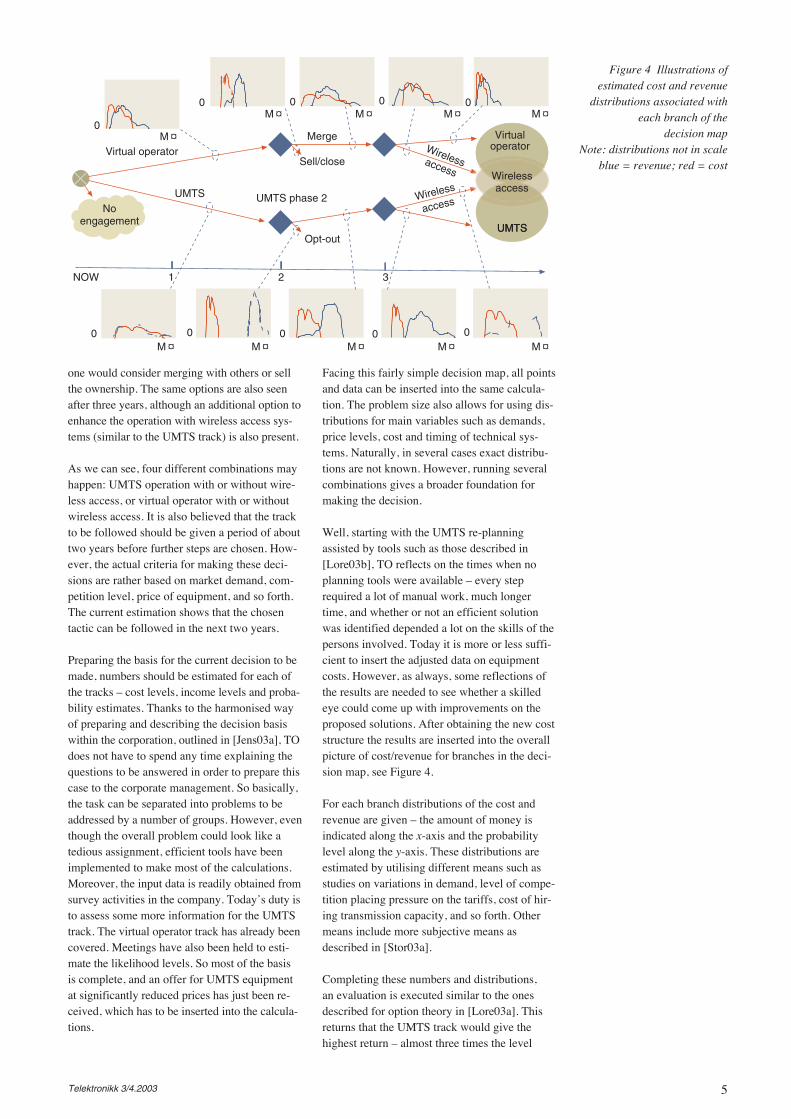
Well, starting with the UMTS re-planningassisted by tools such as those described in[Lore03b], TO reflects on the times when noplanning tools were available – every steprequired a lot of manual work, much longertime, and whether or not an efficient solutionwas identified depended a lot on the skills of thepersons involved. Today it is more or less suffi-cient to insert the adjusted data on equipmentcosts. However, as always, some reflections ofthe results are needed to see whether a skilledeye could come up with improvements on theproposed solutions. After obtaining the new coststructure the results are inserted into the overallpicture of cost/revenue for branches in the deci-sion map, see Figure 4.
For each branch distributions of the cost andrevenue are given – the amount of money isindicated along the x-axis and the probabilitylevel along the y-axis. These distributions areestimated by utilising different means such asstudies on variations in demand, level of compe-tition placing pressure on the tariffs, cost of hir-ing transmission capacity, and so forth. Othermeans include more subjective means asdescribed in [Stor03a].
Completing these numbers and distributions,an evaluation is executed similar to the onesdescribed for option theory in [Lore03a]. Thisreturns that the UMTS track would give thehighest return – almost three times the level
Figure 4 Illustrations ofestimated cost and revenue
distributions associated witheach branch of the
decision mapNote: distributions not in scale
blue = revenue; red = cost
0 0 0
0 00
0
M ¤0
0
0
Virtual operator
UMTS
Merge
Sell/close
UMTS phase 2No
engagement
NOW 1 2 3
Opt-out
M ¤
M ¤ M ¤ M ¤
M ¤ M ¤ M ¤ M ¤ M ¤
UMTSUMTS
Virtualoperator
Wirelessaccess
Wirelessaccess
Wireless
access
6 Telektronikk 3/4.2003
obtained if the virtual operator track were to befollowed.
Although this could be run more or less mechan-ically, it is essential to have some additionalthoughts on the case. TO’s experience in thisfield motivates for further contemplation. Eventhough it is an extensive model, there are alwayssome factors that are not fully captured. In thiscase there is a bill underway to the NationalAssembly of Awayland proposing to lift therequirement that data on the country’s residentscannot be stored in a base abroad. In case this islifted common bases can be utilised for severalcountries, further reducing the cost level. An-other factor is that a general agreement with anequipment manufacturer may be finalised, alsoallowing for lower equipment and operationcosts for the network operator. Both these fac-tors are to be settled within the coming month.Settling these may eliminate some uncertainties,hence TO forwards a recommendation to themanagement board to postpone the decision.
On the other hand, the decision to go for a UMTSroll-out could be made based on the availableresults. However, there is no need to push throughsuch a decision as there is enough lead-time in theplans to wait for about three months.
The complete documentation set together witha short note explaining the recommendation isfinalised and submitted for the board’s meetingnext Monday. “Well, better be prepared forwhat may be decided next month,” TO thinkswhile swiftly going through the e-mails thathave appeared during this morning’s exercise.
Then, it’s time for lunch …
Lunch MeetingThe small delegation from the Ministry appearsin the lobby. As reservations have been made atthe restaurant TO guides the group to thereserved seats. Well, perhaps one should avoidthe pancakes for lunch although this morning’spoint could be applied. One could say that thelunch table is rigged in such a way that a screenis placed close by – “accidentally” running a
slide show close to the topic to be brought up.Basically two issues are expected; firstly mis-conceptions regarding industry trends and glob-alisation, secondly the social effect of flat rates.
Without going into detail in the conversations,the pancake example comes in handy for the lat-ter topic just as a few visual illustrations flash onthe nearby screen. The documentation preparedproviding examples of TO’s view on these mat-ters is also well received. Nice to have collectedreferences from industry magazines and variousstatements – you never know when these can beapplied.
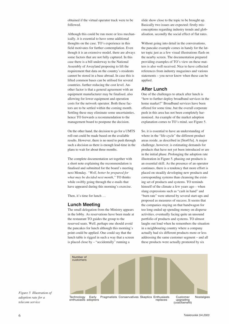
After LunchOne of the challenges to attack after lunch is“how to further deploy broadband services in thehome market?” Broadband services have beenoffered for some time, but the overall corporatepush in this area has not been completely har-monised. An example of the market adoptionexplanation comes to TO’s mind, see Figure 5.
So, it is essential to have an understanding ofwhere in the “life-cycle” the different productareas reside, as described in [Stor03a]. A majorchallenge, however, is estimating demands forproducts that have not yet been introduced or arein the initial phase. Prolonging the adoption rateillustration in Figure 5, phasing out products isan essential skill. As the presence of an operatorcontinues, there is a tendency that more effort isplaced on steadily developing new products andcorresponding systems than cleansing the exist-ing set of products and systems. TO remindshimself of the climate a few years ago – whenslang expressions such as “cash in hand” and“burn rate” were uttered by several start-ups andproposed as measures of success. It seems thatthe companies staying on that bandwagon fortoo long ended up spending money on disperseactivities, eventually facing quite an unsoundportfolio of products and systems. TO almostlaughs out loud when he remembers the situationin a neighbouring country where a companyactually had six different products more or lessaddressing the same customer segment – and allthese products were actually promoted by six
Figure 5 Illustration ofadoption rate for atelecom service
Technologyenthusiasts
Earlyadopters
Pragmatists Conservatives Skeptics Enthusiastsreplaces
Customerupgrading
(cost/benefit)
Nostalgies
Number ofcustomers
7Telektronikk 3/4.2003
different sales representatives holding meetingswith the same customers. Well, some diversifi-cation is often good, but too much is surely nothealthy in the long run.
So, returning to today’s task – TO’s companyhas been in the telecom market for some decadesand a necessary product and system washoutwas carried out last year. The main results wereplans to phase out products and systems. Besidesthe direct cost savings obtained when fewer sys-tems are in operation, a dramatic increase inproduct rollout speed is achieved as the develop-ment and deployment procedures are harmon-ised. The effect on the sales side is also begin-ning to pay back as clear market communicationstrengthens reputation.
In order to make decisions on which productand system to remove from the list, a portfoliomanagement perspective was introduced, see[Jens03a]. This allows for including several fac-tors in the decision such as profit level and risks.Moreover, both shorter and longer terms weretaken into account.
Still, while the overall plan is to reduce the num-ber of systems and products, new ones are alsoconsidered. So today the analysis model is to beprepared for a new product group. The mainquestion is whether or not to introduce this prod-uct group and in case the product is to beoffered, how to do that.
In the overall mature market a new productwould cannibalise existing products in somesense. Hence, the motivation is to avoid com-petitors capturing customers, improving theproduction efficiency (reduced costs allowinghigher margins), appearing as an actor in themarket forefront in accordance with trends, andso forth. Then, the evaluations must always con-sider the alternatives as before.
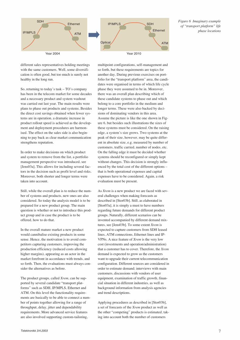
The product groups, called Xrem, can be sup-ported by several candidate “transport plat-forms” such as SDH, IP/MPLS, Ethernet andATM. On this level the functionality require-ments are basically to be able to connect a num-ber of points together allowing for a range ofthroughput, delay, jitter and dependabilityrequirements. More advanced service featuresare also involved supporting custom-tailoring,
multipoint configurations, self-management andso forth, but these requirements are topics foranother day. During previous exercises on port-folio for the “transport platform” area, the candi-dates were organised in terms of which life cyclephase they were assumed to be in. Moreover,there was an overall plan describing which ofthese candidate systems to phase out and whichbelong to a core portfolio in the medium andlonger terms. These were also backed by deci-sions of dominating vendors in this area.Assume the picture is like the one shown in Fig-ure 6, but besides such illustrations the sizes ofthese systems must be considered. On the raisingedge, a system’s size grows. Two systems at thepeak of their size, however, may be quite differ-ent in absolute size, e.g. measured by number ofcustomers, traffic carried, number of nodes, etc.On the falling edge it must be decided whethersystems should be reconfigured or simply keptwithout changes. This decision is strongly influ-enced by the total cost of the different options –that is both operational expenses and capitalexpenses have to be considered. Again, a riskevaluation must be present.
As Xrem is a new product we are faced with sev-eral challenges when making forecasts asdescribed in [Stor03b]. Still, as elaborated in[Stor03a], it is simply a must to have numbersregarding future demands for different productgroups. Naturally, different scenarios can beinvented accompanied by different demand mix-tures, see [Jens03b]. To some extent Xrem isexpected to capture customers from SDH leasedlines, ATM connections, Ethernet lines and IP-VPNs. A nice feature of Xrem is the very lowcost (investments and operation/administration)that a customer has to cover. Therefore, the Xremdemand is expected to grow as the customerswant to upgrade their current telecommunicationconfiguration. Different sources are considered inorder to estimate demand; interviews with maincustomers, discussions with vendors of userequipment, examination of traffic growth, finan-cial situation in different industries, as well asbackground information from analysis agenciesand trend descriptions.
Applying procedures as described in [Stor03b],a set of forecasts of the Xrem product as well asthe other “competing” products is estimated, tak-ing into account both the number of customers
Figure 6 Imaginary exampleof “transport platform” life
phase locationsIP/MPLS
SDH
Year 2004
Ethernet
ATM
Optical
IP/MPLS SDH
Ethernet
ATM
Year 2010
8 Telektronikk 3/4.2003
and the traffic loads. So today’s task is to pre-pare some reasoning around the forecasts. Hav-ing established a corporate approach for fore-casts, TO prepares input for tomorrow’s meetingon these issues. Then the forecasts are to be pre-sented and consequences on other productgroups assessed. This is a significant factor forestimating overall profit improvements of intro-ducing the Xrem product. Other factors are thoseexpressing the costs – both investments andoperational expenses. Having all the variousproduct groups within the corporation, decisionsare to be made on the overall level, which iswhether the overall profit will increase ordecrease.
More challenges are faced because Xrem is anew product and limited information is avail-able. So nearby products are looked at and thediffusion for the demand of Xrem may be esti-mated. Still, the price levels have to be takeninto account arguing for assessing the product(cross) elasticities. The result is a product pene-tration ratio for Xrem. Then, factors providingthe effective traffic loads must also be estimated,as described in [Stor03b]. For each area thenumber of customer sites, average and peakpacket loads, etc. must be found in orderto decide on the effective load and hence theneeded capacity of network nodes and links.
Finding an optimal network design given theeffective load, methods and tools as described in[Lore03b] can be applied. The result is typicallylocations, dimensions and handling of traffic.Several time periods could be considered, possi-bly running a multi-period optimisation algo-rithm. However, in several cases, much uncer-tainty is attached, and a simpler techno-eco-nomic approach could be applied (see e.g.[Stor03a], [Jens03a]) in order to provide a firstassessment of the financial aspects. Treating theuncertainties more systematically, risk manage-ment procedures can be applied as described in[Lore03a] and [Jens03b]. It also needs verifyingthat realising the Xrem product still fits with theoverall network strategy, complying with the setof decisions to be made. However, in case itturns out to be a strong case for realising Xrem,the overall network strategy should be adapted.
“Well, well,” TO thinks – “Having all this pre-defined and an organisation tuned into the sameway of working greatly simplifies the evaluationsand planning activities that need to be under-taken. Having demonstrated the swift work pro-cedure, the top management have gained aninterest in exporting this to other subsidiaries.”
So, there seems to be several options open in thefuture, allowing for more features and concerns tobe incorporated in the work procedure. Returning
his coffee cup to the dishwasher, TO thinks thatbetter insight should be incorporated in phasingout products and networks/systems. In fact,clearer decision criteria for how and when sys-tems should be switched off would greatlyimprove the evaluation procedure. As time goes,it is a lot easier to introduce new systems than toget rid of current systems. As TO takes on theoverall portfolio perspective he thinks that havingall the systems of various levels of success may insome cases be justified. But in most cases it islikely that too much attention from the operationand administration side is spent on less fruitfulsolutions. Again, it is a question of devoting moreattention to the real challenges and allowingprogress to be made in these matters withouttedious managerial bother. For example, shouldone have a steady argument on when to start thedishwasher or which powder to use, the officewould likely run out of clean cups. Moreover, ifthe dishwasher should be restarted every timesomeone returned with a dirty cup, the result ofclean cups would also be delayed.
On his way out TO reflects on the advantages ofhaving clear lines of duties and result handovers.Efficient network planning tasks – from strategyto operational matters – fit very well into thispicture. Similar principles also apply to otherareas of business – and lessons could be learnedfrom those areas. “Keeping one’s eyes and mindopen there is always more to learn,” TO thinks;perhaps examples from the food industry couldbe applied in the telecom industry as well –something to bring up during tomorrow’s “freestyle” discussions?
References[Jens03a] Jensen, T. Network planning – intro-ductory issues. Telektronikk, 99 (3/4), 9–46,2003 (this issue).
[Jens03b] Jensen, T. Network strategy studies.Telektronikk, 99 (3/4), 68–98, 2003 (this issue).
[Lore03a] Lorentzen, R. Portfolio evaluationunder uncertainty. Telektronikk, 99 (3/4),99–109, 2003 (this issue).
[Stor03a] Stordahl, K. Forecasting – an impor-tant factor for network planning. Telektronikk,99 (3/4), 110–121, 2003 (this issue).
[Stor03b] Stordahl, K. Traffic forecasting mod-els for the incumbent based on new drivers inthe market. Telektronikk, 99 (3/4), 122–127,2003 (this issue).
9
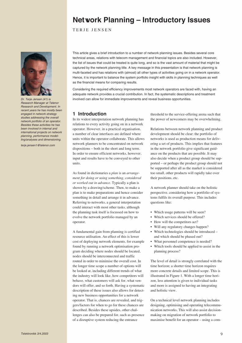
1 IntroductionIn its widest interpretation network planning hasrelations to every activity going on in a networkoperator. However, in a practical organisation,a number of clear interfaces are defined whereunits within the operator collaborate. This allowsnetwork planners to be concentrated on networkdispositions – both in the short and long term.In order to ensure efficient networks, however,input and results have to be conveyed to otherunits.
As found in dictionaries a plan is an arrange-ment for doing or using something, consideredor worked out in advance. Typically a plan isshown by a drawing/scheme. Then, to make aplan is to make preparations and hence considersomething in detail and arrange it in advance.Referring to networks, a general interpretationcould interact with most other tasks, althoughthe planning task itself is focussed on how toevolve the network portfolio managed by anoperator.
A fundamental gain from planning is certifiedresource utilisation. An effect of this is lowercost of deploying network elements, for examplefound by running a network optimisation pro-gram deciding where nodes should be located,nodes should be interconnected and trafficrouted in order to minimise the overall cost. Inthe longer time scope a number of options willbe looked at, including different trends of whatthe industry will look like, how competitors willbehave, what customers will ask for, what ven-dors will offer, and so forth. Having a systematicdescription of these issues also allows for detect-ing new business opportunities for a networkoperator. That is, chances are revealed, and trig-gers/factors for when to go for these chances aredescribed. Besides these upsides, other chal-lenges can also be prepared for, such as presenceof a disruptive system reducing the entrance
threshold to the service-offering arena such thatthe power of newcomers may be overwhelming.
Relations between network planning and productdevelopment should be clear; the portfolio ofnetworks is used as production means for deliv-ering a set of products. This implies that featuresin the network portfolio give significant guid-ance on the products that are possible. It mayalso decide when a product group should be sup-ported – or perhaps the product group should notbe supported after all as the market is consideredtoo small, other products will rapidly take overtheir positions, etc.
A network planner should take on the holisticperspective, considering how a portfolio of sys-tems fulfils its overall purpose. This includesquestions like:
• Which usage patterns will be seen?• Which services should be offered?• How will the competitors act?• Will any regulatory changes happen?• Which technologies should be introduced –
and which should be phased out?• What personnel competence is needed?• Which tools should be applied to assist in the
planning process?
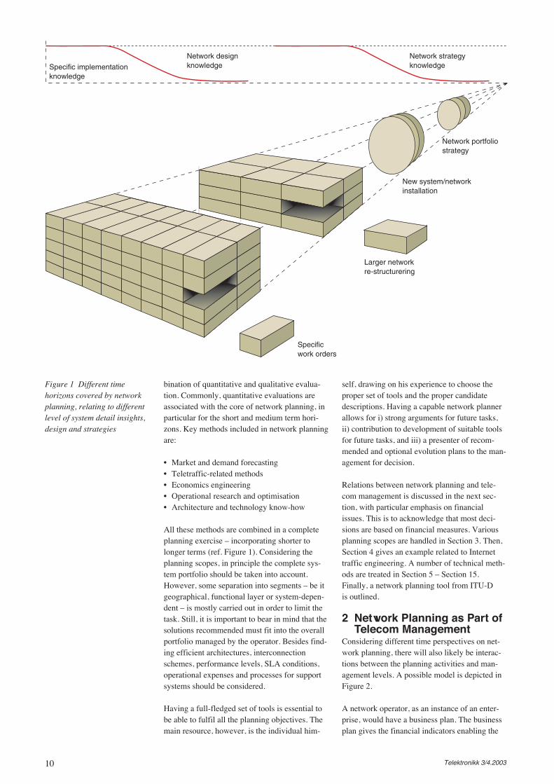
The level of detail is strongly correlated with thetime horizon; a shorter time horizon requiresmore concrete details and limited scope. This isillustrated in Figure 1. With a longer time hori-zon, less attention is given to individual tasksand more is assigned to having an integratingand holistic view.
On a technical level network planning includesdesigning, optimising and operating telecommu-nication networks. This will also assist decision-making on migration of network portfolio tomaximise benefit for an operator – using a com-
Network Planning – Introductory IssuesT E R J E J E N S E N
This article gives a brief introduction to a number of network planning issues. Besides several core
technical areas, relations with telecom management and financial topics are also included. However,
the list of issues that could be treated is quite long, and so is the vast amount of material that might be
captured by the network planning title. A key message in this presentation is that network planning is
multi-faceted and has relations with (almost) all other types of activities going on in a network operator.
Hence, it is important to balance the system portfolio insight with skills in planning techniques as well
as the financial means for comparing results.
Considering the required efficiency improvements most network operators are faced with, having an
adequate network provides a crucial contribution. In fact, the systematic descriptions and treatment
involved can allow for immediate improvements and reveal business opportunities.Dr. Terje Jensen (41) isResearch Manager at TelenorResearch and Development. Inrecent years he has mostly beenengaged in network strategystudies addressing the overallnetwork portfolio of an operator.Besides these activities he hasbeen involved in internal andinternational projects on networkplanning, performance model-ling/analyses and dimensioning.
Telektronikk 3/4.2003
10 Telektronikk 3/4.2003
bination of quantitative and qualitative evalua-tion. Commonly, quantitative evaluations areassociated with the core of network planning, inparticular for the short and medium term hori-zons. Key methods included in network planningare:
• Market and demand forecasting• Teletraffic-related methods• Economics engineering• Operational research and optimisation• Architecture and technology know-how
All these methods are combined in a completeplanning exercise – incorporating shorter tolonger terms (ref. Figure 1). Considering theplanning scopes, in principle the complete sys-tem portfolio should be taken into account.However, some separation into segments – be itgeographical, functional layer or system-depen-dent – is mostly carried out in order to limit thetask. Still, it is important to bear in mind that thesolutions recommended must fit into the overallportfolio managed by the operator. Besides find-ing efficient architectures, interconnectionschemes, performance levels, SLA conditions,operational expenses and processes for supportsystems should be considered.
Having a full-fledged set of tools is essential tobe able to fulfil all the planning objectives. Themain resource, however, is the individual him-
self, drawing on his experience to choose theproper set of tools and the proper candidatedescriptions. Having a capable network plannerallows for i) strong arguments for future tasks,ii) contribution to development of suitable toolsfor future tasks, and iii) a presenter of recom-mended and optional evolution plans to the man-agement for decision.
Relations between network planning and tele-com management is discussed in the next sec-tion, with particular emphasis on financialissues. This is to acknowledge that most deci-sions are based on financial measures. Variousplanning scopes are handled in Section 3. Then,Section 4 gives an example related to Internettraffic engineering. A number of technical meth-ods are treated in Section 5 – Section 15.Finally, a network planning tool from ITU-Dis outlined.
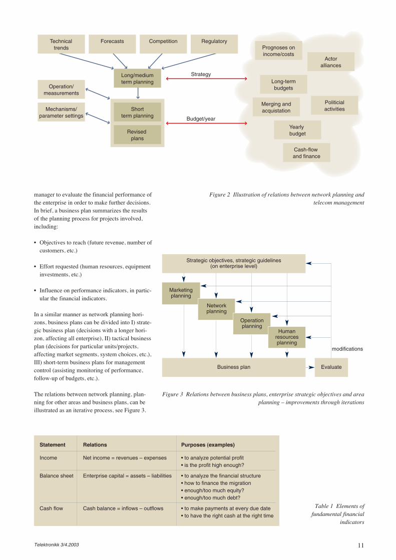
2 Network Planning as Part ofTelecom Management
Considering different time perspectives on net-work planning, there will also likely be interac-tions between the planning activities and man-agement levels. A possible model is depicted inFigure 2.
A network operator, as an instance of an enter-prise, would have a business plan. The businessplan gives the financial indicators enabling the
Figure 1 Different timehorizons covered by networkplanning, relating to differentlevel of system detail insights,design and strategies
Specific implementationknowledge
Network designknowledge
Network strategyknowledge
Network portfoliostrategy
New system/network installation
Larger network re-structurering
Specific work orders
11Telektronikk 3/4.2003
manager to evaluate the financial performance ofthe enterprise in order to make further decisions.In brief, a business plan summarizes the resultsof the planning process for projects involved,including:
• Objectives to reach (future revenue, number ofcustomers, etc.)
• Effort requested (human resources, equipmentinvestments, etc.)
• Influence on performance indicators, in partic-ular the financial indicators.
In a similar manner as network planning hori-zons, business plans can be divided into I) strate-gic business plan (decisions with a longer hori-zon, affecting all enterprise), II) tactical businessplan (decisions for particular units/projects,affecting market segments, system choices, etc.),III) short-term business plans for managementcontrol (assisting monitoring of performance,follow-up of budgets, etc.).
The relations between network planning, plan-ning for other areas and business plans, can beillustrated as an iterative process, see Figure 3.
Figure 2 Illustration of relations between network planning and telecom management
Statement Relations Purposes (examples)
Income Net income = revenues – expenses • to analyze potential profit• is the profit high enough?
Balance sheet Enterprise capital = assets – liabilities • to analyze the financial structure• how to finance the migration• enough/too much equity?• enough/too much debt?
Cash flow Cash balance = inflows – outflows • to make payments at every due date• to have the right cash at the right time
Table 1 Elements offundamental financial
indicators
Technicaltrends
Forecasts Competition Regulatory
Strategy
Budget/year
Prognoses onincome/costs
Actoralliances
Long-termbudgetsOperation/
measurements
Long/mediumterm planning
Merging andacquistation
PoliticialactivitiesMechanisms/
parameter settingsShort
term planning
Yearly budgetRevised
plans
Cash-flow and finance
Strategic objectives, strategic guidelines(on enterprise level)
EvaluateBusiness plan
modifications
Figure 3 Relations between business plans, enterprise strategic objectives and areaplanning – improvements through iterations
Marketingplanning
Networkplanning
Operationplanning
Humanresourcesplanning
12 Telektronikk 3/4.2003
Besides the outer iteration, there may also beinteractions between the different planninggroups. However, a fundamental message is thatthese have to be coherent in order to efficientlysupport the enterprise’s objectives.
The elements in the business plan contain finan-cial indicators, models for costs and revenues aswell as sensitivity studies. These may be updatedduring planning exercises, both parameter rangesand modelling considerations; through evalua-tion of effects from activities, change of techni-cal/organization/etc. solutions, portfolio adjust-ments, strength-weakness-opportunities-threatsanalyses, and so forth. As shown in the figure,iterations allows for steady improvements.
It is hard to describe business plans and businessmodelling without entering an arena of financialindicators. All fundamental financial indicatorsare carried out with elements as given in Table 1.
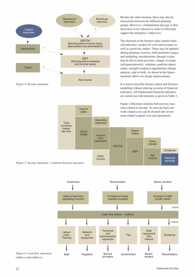
Figure 4 illustrates relations between key mea-sures related to income. As seen the basic net-work-related costs can be divided into invest-ment-related (capital cost) and operational
Capitalexpenses
Operationalexpenses
Revenues(top-line)
Depreciation
EBITDA(Earning before income taxes, depreciation and amortisation)
EBIT(Earning before interests
and income taxes)
Net income
Taxes
–
–
– +
Figure 4 Income statement
Otherincome
Operatingexpenses
Incomefrom
operations
Retainedearnings
Dividends
Cost ofsales
Netincome
Taxes,interest
EBIT
Depre-ciation
Grossmargin
EBITDA
Totalrevenues
(sales/top-line)
Figure 5 Income statement – relations between measures
Sales of services(operating income)
Customers Shareholders Banks, lenders
Inflows
Outflows
Labourcosts,
Training
Staff
Networkand
equipment
Suppliers
Technicaland
administrativeexpenses
Serviceproviders
Tax
Government
Debtrepayment
withinterest
Banks,lenders
Dividends
Shareholders
Increase of equity(capital increase)
Increase of debt(credit, loans)
Cash flow (inflow – outflow)
Figure 6 Cash flow statement(inflows and outflows)
13Telektronikk 3/4.2003
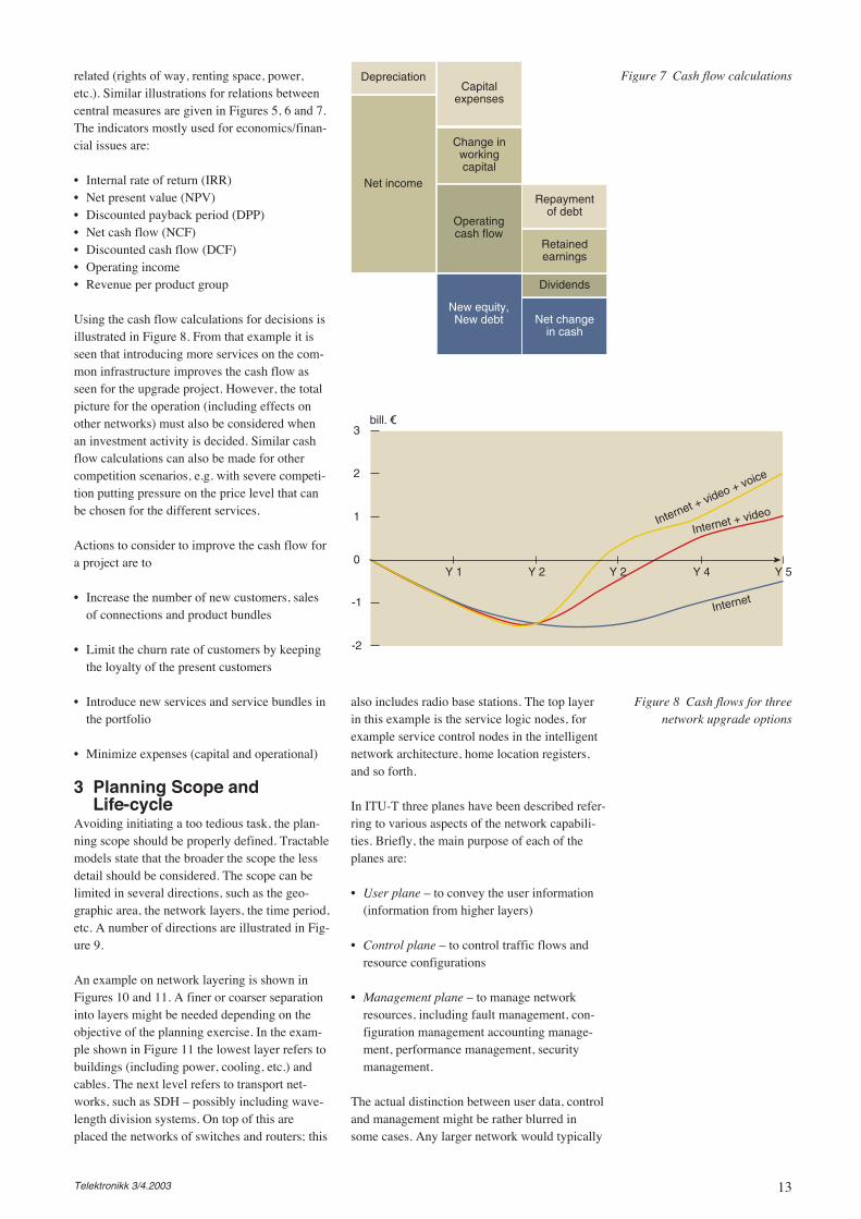
related (rights of way, renting space, power,etc.). Similar illustrations for relations betweencentral measures are given in Figures 5, 6 and 7.The indicators mostly used for economics/finan-cial issues are:
• Internal rate of return (IRR)• Net present value (NPV)• Discounted payback period (DPP)• Net cash flow (NCF)• Discounted cash flow (DCF)• Operating income• Revenue per product group
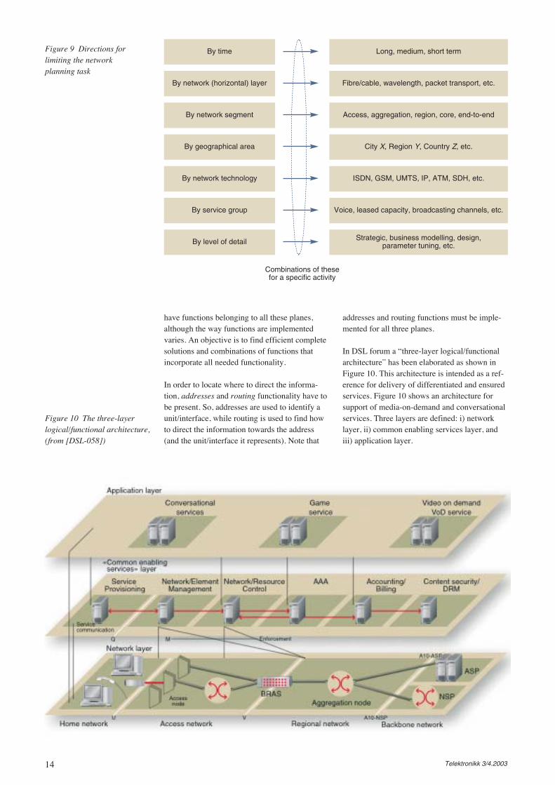
Using the cash flow calculations for decisions isillustrated in Figure 8. From that example it isseen that introducing more services on the com-mon infrastructure improves the cash flow asseen for the upgrade project. However, the totalpicture for the operation (including effects onother networks) must also be considered whenan investment activity is decided. Similar cashflow calculations can also be made for othercompetition scenarios, e.g. with severe competi-tion putting pressure on the price level that canbe chosen for the different services.
Actions to consider to improve the cash flow fora project are to
• Increase the number of new customers, salesof connections and product bundles
• Limit the churn rate of customers by keepingthe loyalty of the present customers
• Introduce new services and service bundles inthe portfolio
• Minimize expenses (capital and operational)
3 Planning Scope andLife-cycle
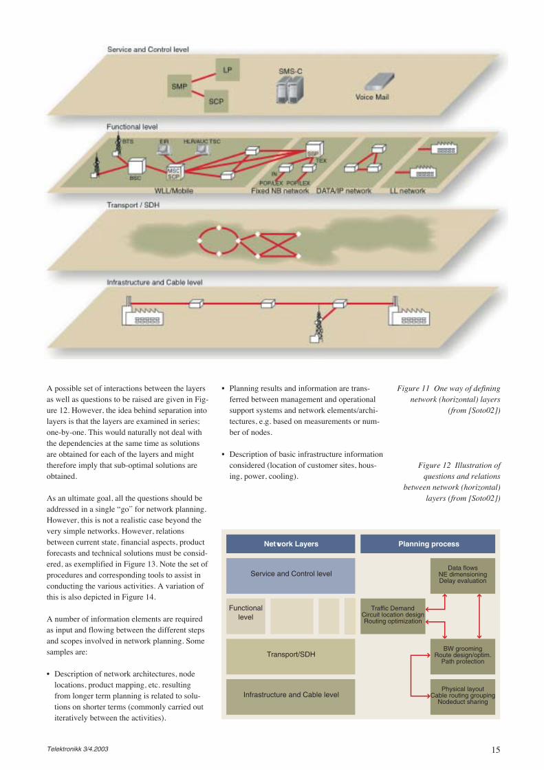
Avoiding initiating a too tedious task, the plan-ning scope should be properly defined. Tractablemodels state that the broader the scope the lessdetail should be considered. The scope can belimited in several directions, such as the geo-graphic area, the network layers, the time period,etc. A number of directions are illustrated in Fig-ure 9.
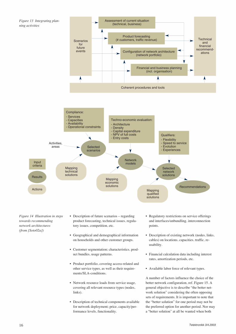
An example on network layering is shown inFigures 10 and 11. A finer or coarser separationinto layers might be needed depending on theobjective of the planning exercise. In the exam-ple shown in Figure 11 the lowest layer refers tobuildings (including power, cooling, etc.) andcables. The next level refers to transport net-works, such as SDH – possibly including wave-length division systems. On top of this areplaced the networks of switches and routers; this
also includes radio base stations. The top layerin this example is the service logic nodes, forexample service control nodes in the intelligentnetwork architecture, home location registers,and so forth.
In ITU-T three planes have been described refer-ring to various aspects of the network capabili-ties. Briefly, the main purpose of each of theplanes are:
• User plane – to convey the user information(information from higher layers)
• Control plane – to control traffic flows andresource configurations
• Management plane – to manage networkresources, including fault management, con-figuration management accounting manage-ment, performance management, securitymanagement.
The actual distinction between user data, controland management might be rather blurred insome cases. Any larger network would typically
Figure 8 Cash flows for threenetwork upgrade options
Net income
DepreciationCapital
expenses
Change inworkingcapital
Operatingcash flow
New equity,New debt
Repaymentof debt
Retainedearnings
Dividends
Net changein cash
Figure 7 Cash flow calculations
Internet + video + voice
Internet + video
Internet-1
0
1
2
3
-2
Y 1 Y 2 Y 2 Y 4 Y 5
14 Telektronikk 3/4.2003
have functions belonging to all these planes,although the way functions are implementedvaries. An objective is to find efficient completesolutions and combinations of functions thatincorporate all needed functionality.
In order to locate where to direct the informa-tion, addresses and routing functionality have tobe present. So, addresses are used to identify aunit/interface, while routing is used to find howto direct the information towards the address(and the unit/interface it represents). Note that
addresses and routing functions must be imple-mented for all three planes.
In DSL forum a “three-layer logical/functionalarchitecture” has been elaborated as shown inFigure 10. This architecture is intended as a ref-erence for delivery of differentiated and ensuredservices. Figure 10 shows an architecture forsupport of media-on-demand and conversationalservices. Three layers are defined: i) networklayer, ii) common enabling services layer, andiii) application layer.
By time Long, medium, short term
Fibre/cable, wavelength, packet transport, etc.
Access, aggregation, region, core, end-to-end
City X, Region Y, Country Z, etc.
ISDN, GSM, UMTS, IP, ATM, SDH, etc.
Voice, leased capacity, broadcasting channels, etc.
Strategic, business modelling, design, parameter tuning, etc.
By network (horizontal) layer
By network segment
By geographical area
By network technology
By service group
By level of detail
Combinations of thesefor a specific activity
Figure 9 Directions forlimiting the networkplanning task
Figure 10 The three-layerlogical/functional architecture,(from [DSL-058])
15Telektronikk 3/4.2003
A possible set of interactions between the layersas well as questions to be raised are given in Fig-ure 12. However, the idea behind separation intolayers is that the layers are examined in series;one-by-one. This would naturally not deal withthe dependencies at the same time as solutionsare obtained for each of the layers and mighttherefore imply that sub-optimal solutions areobtained.
As an ultimate goal, all the questions should beaddressed in a single “go” for network planning.However, this is not a realistic case beyond thevery simple networks. However, relationsbetween current state, financial aspects, productforecasts and technical solutions must be consid-ered, as exemplified in Figure 13. Note the set ofprocedures and corresponding tools to assist inconducting the various activities. A variation ofthis is also depicted in Figure 14.
A number of information elements are requiredas input and flowing between the different stepsand scopes involved in network planning. Somesamples are:
• Description of network architectures, nodelocations, product mapping, etc. resultingfrom longer term planning is related to solu-tions on shorter terms (commonly carried outiteratively between the activities).
• Planning results and information are trans-ferred between management and operationalsupport systems and network elements/archi-tectures, e.g. based on measurements or num-ber of nodes.
• Description of basic infrastructure informationconsidered (location of customer sites, hous-ing, power, cooling).
Figure 11 One way of definingnetwork (horizontal) layers
(from [Soto02])
Figure 12 Illustration ofquestions and relations
between network (horizontal)layers (from [Soto02])
Planning processNetwork Layers
Data flowsNE dimensioningDelay evaluation
Service and Control level
Traffic DemandCircuit location designRouting optimization
Functionallevel
BW groomingRoute design/optim.
Path protectionTransport/SDH
Physical layoutCable routing grouping
Nodeduct sharingInfrastructure and Cable level
16 Telektronikk 3/4.2003
• Description of future scenarios – regardingproduct forecasting, technical issues, regula-tory issues, competition, etc.
• Geographical and demographical informationon households and other customer groups.
• Customer segmentation; characteristics, prod-uct bundles, usage patterns.
• Product portfolio, covering access-related andother service types, as well as their require-ments/SLA-conditions.
• Network resource loads from service usage,covering all relevant resource types (nodes,links).
• Description of technical components availablefor network deployment; price, capacity/per-formance levels, functionality.
• Regulatory restrictions on service offeringsand interfaces/unbundling, interconnectionpoints.
• Description of existing network (nodes, links,cables) on locations, capacities, traffic, re-usability.
• Financial calculation data including interestrates, amortization periods, etc.
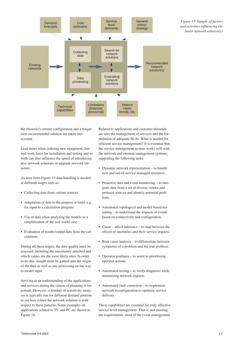
• Available labor force of relevant types.
A number of factors influence the choice of thebetter network configuration, ref. Figure 15. Ageneral objective is to describe “the better net-work solution” considering the often opposingsets of requirements. It is important to note thatthe “better solution” for one period may not bethe preferred option for another period. Nor maya “better solution” at all be wanted when both
Scenarios for
futureevents
Technicaland
financialrecommend-
ations
Assessment of current situation(technical, business)
Product forecasting(# customers, traffic revenue)
Configuration of network architecture(network portfolio)
Financial and business planning(incl. organisation)
Coherent procedures and tools
Figure 13 Integrating plan-ning activities
Actions
Mappingtechnicalsolutions
Activities,areas
Mappingeconomicsolutions
Mappingqualifiedsolutions
Compliance:- Services- Capacities- Availability- Operational constraints
Techno-economic evaluation:- Architecture- Density- Capital expenditure- NPV of full costs- Entry costs
Qualifiers:- Flexibility- Speed to service- Evolution- Experiences
Inputcriteria
Results
Selectedscenarios
Networkmodels
Selectednetworksolutions
Recommendations
Figure 14 Illustration in stepstowards recommendingnetwork architectures(from [Soto02a])
17Telektronikk 3/4.2003
the (historic/) current configuration and a longerterm recommended solution are taken intoaccount.
Lead times when ordering new equipment, lim-ited work force for installation and testing and soforth can also influence the speed of introducingnew network solutions or upgrade network ele-ments.
As seen from Figure 15 data handling is neededat different stages such as:
• Collecting data from various sources
• Adaptation of data to the purpose at hand, e.g.for input to a calculation program
• Use of data when analysing the models as asimplification of the real world case
• Evaluation of results/output data from the cal-culations.
During all these stages, the data quality must beassessed, including the uncertainty attached andwhich values are the most likely ones. In orderto do this, insight must be gained into the originof the data as well as any processing on the wayto model input.
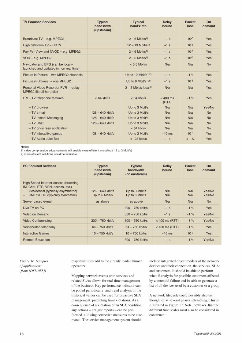
Arriving at an understanding of the applicationsand services during the course of planning is im-portant. However, a number of sensitivity analy-ses is typically run for different demand patternsto see how robust the network solution is withrespect to these patterns. Some examples onapplications related to TV and PC are shown inFigure 16.
Related to applications and customer demandsare also the management of services and the for-mulation of adequate SLAs. What is needed forefficient service management? It is essential thatthe service management system works well withthe network and element management systems,supporting the following tasks:
• Dynamic network representation – to handlenew and out-of-service managed resources.
• Proactive data and event monitoring – to inte-grate data from a set of diverse vendor andprotocol sources and identify potential prob-lems.
• Automated topological and model-based rea-soning – to understand the impacts of eventsbased on connectivity and configuration.
• Cause – effect inference – to map between theeffects of anomalies and their service impacts.
• Root cause analysis – to differentiate betweensymptoms of a problem and the true problem.
• Operator guidance – to assist to prioritisingoperator actions.
• Automated testing – to verify diagnoses whileminimizing network impacts.
• Automated fault correction – to implementnetwork reconfiguration to optimise servicedelivery.
These capabilities are essential for truly effectiveservice level management. That is, not meetingthe requirements, most of the event management
Demandforecasts
Technicalcapabilities
Limitations(financial,personnel)
Historicviews,
trends, etc.
Existingnetworks
Recommendednetwork
solution(s)
Collectingdata
Search fornetworksolutions
Evaluatingnetworksolutions
Dataprocessing
Costestimates
Servicelevel
demands
Generalpolicy/
strategy
Figure 15 Sample of factorsand activities influencing the
better network solution(s)
18 Telektronikk 3/4.2003
responsibilities add to the already loaded humanoperators.
Mapping network events onto services andrelated SLAs allows for real-time managementof the business. Key performance indicator canbe polled periodically, and trend analysis of thehistorical values can be used for proactive SLAmanagement, predicting limit violations. As aconsequence of a violation of an SLA condition,any actions – not just reports – can be per-formed, allowing corrective measures to be auto-mated. The service management system should
include integrated object models of the networkdevices and their connection, the services, SLAsand customers. It should be able to performwhat-if analysis for possible customers affectedby a potential failure and be able to generate alist of all devices used by a customer or a group.
A network lifecycle could possibly also bethought of as several phases interacting. This isillustrated in Figure 17. Note, however, that thedifferent time scales must also be considered incoherence.
TV Focused Services Typical Typical Delay Packet Onbandwidth bandwidth bound loss demand(upstream)
Broadcast TV – e.g. MPEG2 2 – 6 Mbit/s1) ~1 s 10-5 Yes
High definition TV – HDTV 12 – 19 Mbit/s1) ~1 s 10-5 Yes
Pay Per View and NVOD – e.g. MPEG2 2 – 6 Mbit/s1) ~1 s 10-5 Yes
VOD – e.g. MPEG2 2 – 6 Mbit/s1) ~1 s 10-5 Yes
Navigator and EPG (can be locally < 0.5 Mbit/s N/a N/a Nolaunched and updated in non real time)
Picture in Picture – two MPEG2 channels Up to 12 Mbit/s1,2) ~1 s ~1 % Yes
Picture in Browser – one MPEG2 Up to 9 Mbit/s1,2) ~1 s 10-5 Yes
Personal Video Recorder PVR – replay 2 – 6 Mbit/s local1) N/a N/a YesMPEG2 file off hard disk
ITV – TV telephone features < 64 kbit/s < 64 kbit/s < 400 ms ~1 % Yes(RTT)
– TV browser Up to 3 Mbit/s N/a N/a Yes/No
– TV e-mail 128 – 640 kbit/s Up to 3 Mbit/s N/a N/a No
– TV Instant Messaging 128 – 640 kbit/s Up to 3 Mbit/s N/a N/a No
– TV Chat 128 – 640 kbit/s Up to 3 Mbit/s N/a N/a No
– TV on-screen notification < 64 kbit/s N/a N/a No
– TV interactive games 128 – 640 kbit/s Up to 3 Mbit/s ~10 ms 10-5 Yes
– TV Audio Juke Box < 128 kbit/s ~1 s < 1 % Yes
Notes:1) video compression advancements will enable more efficient encoding (1.5 to 3 Mbit/s)2) more efficient solutions could be available
PC Focused Services Typical Typical Delay Packet Onbandwidth bandwidth bound loss demand(upstream) (downstream)
High Speed Internet Access (browsing,IM, Chat, FTP, VPN, access, etc.)– Residential (typically asymmetric) 128 – 640 kbit/s Up to 3 Mbit/s N/a N/a Yes/No– SME/SOHO (typically symmetric) Up to 6 Mbit/s Up to 6 Mbit/s N/a N/a Yes/No
Server based e-mail as above as above N/a N/a No
Live TV on PC 300 – 750 kbit/s ~1 s ~1 % Yes
Video on Demand 300 – 750 kbit/s ~1 s ~1 % Yes/No
Video Conferencing 300 – 750 kbit/s 300 – 750 kbit/s < 400 ms (RTT) ~1 % Yes/No
Voice/Video telephony 64 – 750 kbit/s 64 – 750 kbit/s < 400 ms (RTT) ~1 % Yes
Interactive Games 10 – 750 kbit/s 10 – 750 kbit/s ~10 ms 10-5 Yes
Remote Education 300 – 750 kbit/s ~1 s ~1 % Yes/No
Figure 16 Samples of applications (from [DSL-058])
19Telektronikk 3/4.2003
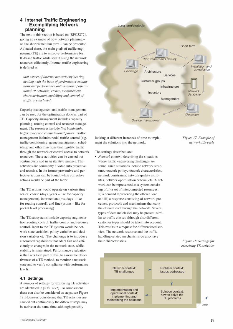
4 Internet Traffic Engineering– Exemplifying Networkplanning
The text in this section is based on [RFC3272],giving an example of how network planning –on the shorter/medium term – can be presented.As stated there, the main goals of traffic engi-neering (TE) are to improve performance forIP-based traffic while still utilising the networkresources efficiently. Internet traffic engineeringis defined as
that aspect of Internet network engineeringdealing with the issue of performance evalua-tions and performance optimisation of opera-tional IP networks. Hence, measurement,characterisation, modelling and control oftraffic are included.
Capacity management and traffic managementcan be used for the optimisation done as part ofTE. Capacity arrangement includes capacityplanning, routing control and resource manage-ment. The resources include link bandwidth,buffer space and computational power. Trafficmanagement includes nodal traffic control (e.g.traffic conditioning, queue management, sched-uling) and other functions that regulate trafficthrough the network or control access to networkresources. These activities can be carried outcontinuously and in an iterative manner. Theactivities are commonly divided into proactiveand reactive. In the former preventive and per-fective actions can be found, while correctiveactions would be part of the latter.
The TE actions would operate on various timescales; coarse (days, years – like for capacitymanagement), intermediate (ms, days – likefor routing control), and fine (ps, ms – like forpacket level processing).
The TE subsystems include capacity augmenta-tion, routing control, traffic control and resourcecontrol. Input to the TE system would be net-work state variables, policy variables and deci-sion variables etc. The challenge is to introduceautomated capabilities that adapt fast and effi-ciently to changes in the network state, whilestability is maintained. Performance evaluationis then a critical part of this, to assess the effec-tiveness of a TE method, to monitor a networkstate and to verify compliance with performancelevels.
4.1 SettingsA number of settings for exercising TE activitiesare identified in [RFC3272]. To some extentthese can also be considered as steps, see Figure18. However, considering that TE activities arecarried out continuously the different steps maybe active at the same time, although possibly
looking at different instances of time to imple-ment the solutions into the network.
The settings described are:• Network context; describing the situations
where traffic engineering challenges arefound. Such situations include network struc-ture, network policy, network characteristics,network constraints, network quality attrib-utes, network optimisation criteria, etc. A net-work can be represented as a system consist-ing of, i) a set of interconnected resources,ii) a demand representing the offered load,and iii) a response consisting of network pro-cesses, protocols and mechanisms that carrythe offered load through the network. Severaltypes of demand classes may be present, simi-lar to traffic classes although also differentcustomer types should be taken into account.This results in a request for differentiated ser-vice. The network resource and the traffichandling-related mechanisms do also havetheir characteristics.
Figure 17 Example of network life-cycle
ArchitectureRe-design
Procurement and delivery
Installation and commission
Networkdatabase
Service management
Operation
Long term/strategic
Short term
Services
Customer groups
Infrastructure
Inventory
Management
Network context:TE challenges
Problem context:issues addressed
Solution context:how to solve the
TE problems
Implementation andoperational context:implementing and
maintaining the solutions
time
Figure 18 Settings forexercising TE activities
20 Telektronikk 3/4.2003
• Problem context; defining the issues that TEaddresses, like identification, abstraction, rep-resentation, formulation, requirement specifi-cation, solution space specification, etc. Oneclass of problems is how to formulate thequestions that traffic engineering shouldsolve; how to describe requirements on thesolution space, how to describe desirable fea-tures of good solutions, how to solve the prob-lems and how to characterise and measure theeffectiveness of the solutions. Another prob-lem is how to measure and assess the networkstate parameters, including the network topol-ogy. A third class of problems is how to char-acterise and evaluate network states under avariety of scenarios. This can be addressedboth on system level (macro states – “macroTE”) and resource level (micro state – “microTE”). Solving congestion is an essential partof performance improvement. Handling con-gestion can be divided into demand side poli-cies (restrictive) and supply side policies(expansive).
• Solution context; elaborating how to solvethe TE problems. This typically means evalua-tion of alternatives, which requires estimatingtraffic load, characterising network state, elab-orating solutions on TE problems and settingup a set of control actions. The instrumentsrelevant include i) a set of policies, objectivesand requirements for network performanceevaluation and optimisation, ii) a set of toolsand mechanisms for measurement, characteri-sation, modelling and controlling traffic andallocation to network resources, iii) a set ofconstraints on the operating environment, net-work protocols and TE system, iv) a set ofquantitative and qualitative techniques and
methods for abstracting, formulating and solv-ing TE problems, v) a set of administrativecontrol parameters that may be managed bya configuration management system, vi) a setof guidelines for network performance evalua-tion, optimisation/improvement. Traffic esti-mates can be derived from customer subscrip-tion information, traffic projections, trafficmodels, and from empirical measurements.Polices for handling the congestion problemcan be categorised according to the criteriai) response time scale (long – weeks tomonths, e.g. capacity planning; medium –minutes to days, e.g. setting routing parame-ters, adjusting Label Switched Path (LSP)design; short – ps to minutes, e.g. packet pro-cessing of marking, queue management),ii) reactive versus preventive, and iii) supplyside (increase available capacity, redistributetraffic flows) versus demand side (control theoffered traffic).
• Implementation and operational context;implementing the actual solutions, involvingplanning (e.g. a priori determined actionsbased on triggers), organisation (e.g. assigningresponsibilities to different units and co-ordi-nating activities), and execution (e.g. measure-ment and application of corrective and perfec-tive actions).
These context descriptions may also be lookedupon as gradually getting more precise andcloser to the implementation.
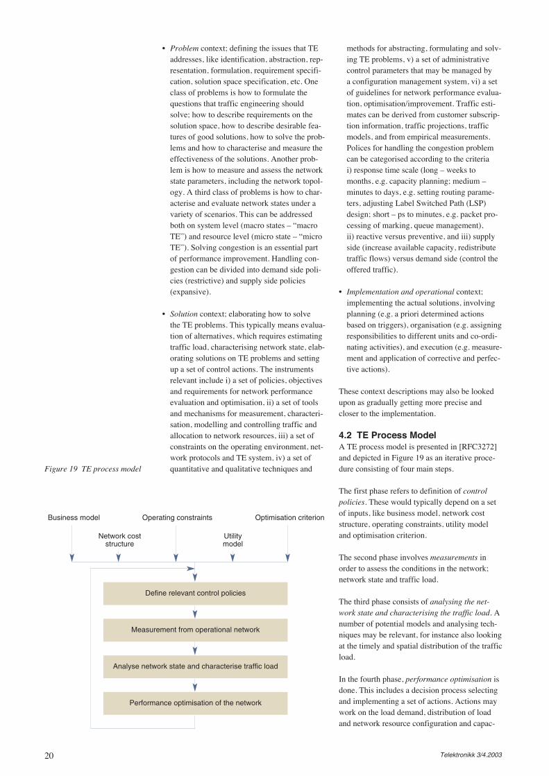
4.2 TE Process ModelA TE process model is presented in [RFC3272]and depicted in Figure 19 as an iterative proce-dure consisting of four main steps.
The first phase refers to definition of controlpolicies. These would typically depend on a setof inputs, like business model, network coststructure, operating constraints, utility modeland optimisation criterion.
The second phase involves measurements inorder to assess the conditions in the network;network state and traffic load.
The third phase consists of analysing the net-work state and characterising the traffic load. Anumber of potential models and analysing tech-niques may be relevant, for instance also lookingat the timely and spatial distribution of the trafficload.
In the fourth phase, performance optimisation isdone. This includes a decision process selectingand implementing a set of actions. Actions maywork on the load demand, distribution of loadand network resource configuration and capac-
Business model
Network coststructure
Utilitymodel
Operating constraints Optimisation criterion
Define relevant control policies
Measurement from operational network
Analyse network state and characterise traffic load
Performance optimisation of the network
Figure 19 TE process model
21Telektronikk 3/4.2003
ity. This may also initiate a network planning inorder to improve network design, capacity, tech-nology, and element configuration.
4.3 TE Key ComponentsThe key components of the TE process modelare:
• Measurement subsystem: Carrying out mea-surement is essential to provide feedback onthe system state and performance. It is alsocritical in order to assess the service level pro-vided (and QoS) and effect of TE actions. Abasic distinction between monitoring andevaluation is to be observed; monitoring refersto provision of raw data, while evaluationrefers to use of the raw data for inferring onthe system state and performance. Measure-ments can be carried out at different levels ofaggregation, e.g. packet level, flow level, userlevel, traffic aggregate level, component level,network-wide level, and so forth. In order toperform measurements systematically, severalquestions have to be answered, like[RFC3272]: Which parameters are to bemeasured? How should the measurementsbe accomplished? Where should the measure-ment be performed? When should the mea-surement be performed? How frequentlyshould the monitored variables be measured?What level of measurement accuracy and reli-ability is desirable and realistic? To whatextent can the measurement system permissi-bly interfere with the operational network con-ditions? What is the acceptable cost of mea-surements?
• Modelling and analysis subsystem: A centralpart of the modelling is to elaborate a represen-tation of the relevant traffic characteristics andnetwork behaviour. In case a structural modelis used, the organisation of the network and itscomponents are the main emphasis. Whenbehavioural models are used, the dynamics ofthe network and traffic are the key issues. Thelatter model is particularly relevant whendoing performance studies. Then adequatemodels of the traffic sources are also needed.
• Optimisation subsystem: Optimisation can becategorised as real-time and non-real-time.The former operates on short to medium timescales (e.g. ms to hours) and works to adjustparameters in mechanisms in order to relievecongestion and improve performance. Exam-ples of means are tuning of routing parame-ters, tuning of buffer management mecha-nisms and changing Label Switched Paths(LSPs). Non-real-time is also seen as networkplanning, typically working on a longer scale.For both of these, stability and robustness areessential concerns.
Routing is a central component in efficient han-dling of traffic flows in an IP-based network.When introducing a number of service classes,some additional constraints can also be consid-ered when deciding upon the possible routing.Examples of such constraints are available band-width, hop count, and delay. This implies thatpossible paths as seen from a router must havethe corresponding attributes attached.
4.4 Requirements on TE Systems[RFC3272] describes a number of requirementsthat a TE system should meet. Here a require-ment is understood as a capability needed tosolve a TE problem or to achieve a TE objective.The requirements are either non-functional orfunctional. A non-functional requirement relatesto the quality attributes of state characteristics ofa TE system. A functional requirement gives thefunction a TE system should perform in order toreach an objective or address a problem.
4.4.1 Non-functional RequirementsThe generic non-functional requirements givenin [RFC3272] are:
• Usability. This is a human factor aspect refer-ring to the ease of deployment and operationof a TE system.
• Automation. Usually, as many functions aspossible should be automated, reducing thehuman effort to control and analyse the infor-mation and network state. This is evenstronger for a larger network.
• Scalability. The TE system should scale wellwhen the number of routers, links, trafficflows, subscribers, etc. grows. This may implythat a scalable TE architecture is applied.
• Stability. This is an essential requirement foran operational system avoiding adverse resultsfor certain combinations of input and stateinformation.
• Flexibility. A TE system should be flexibleboth in terms of the optimisation policy andthe scope. An example of scope is that addi-tional classes should be considered in casethese are introduced into the network. Anotheraspect of flexibility is that some subsystems ofthe TE system could be enabled/disabled.
• Visibility. Mechanisms to collect informationfrom the network elements and analyse thedata have to be present in a TE system. Thesewould then allow for presenting the opera-tional conditions of the network.
• Simplicity. A TE system should be as simpleas possible; that is, considered from the out-
22 Telektronikk 3/4.2003
side, not necessarily using simple algorithms.Simplicity is particularly important for thehuman interface.
• Efficiency. As little demanding as possible, interms of processing and memory resources, isrequested. However, this also refers to the factthat a result from the TE system should beobtained in a timely manner.
• Reliability. A TE system should be availablein the operational state when needed.
• Survivability. Recovering from a failure andmaintaining the operation is requested, in par-ticular for the more critical functions of a TEsystem. Commonly, this requires that someredundancy is introduced.
• Correctness. A correct response (accordingto the algorithms implemented) has to be ob-tained from a TE system.
• Maintainability. It should be simple to main-tain a TE system.
• Extensibility. It should be easy to extend a TEsystem, e.g. when introducing new functionsand when the underlying network is extended.
• Interoperability. Open standards should beused for the interfaces in order to simplifyinteroperation with other systems.
• Security. Means supporting integrity, informa-tion concealment, etc. have to be imple-mented.
As mentioned, some of these requirements maybe mandatory while others are optional for a par-ticular TE system.
4.4.2 Functional RequirementsSome functional requirements are also describedin [RFC3272], such as those related to:
• Routing. An efficient routing system shouldtake both traffic characteristics and networkconstraints into account when deriving thebetter routing schemes. A load splitting ratioamong alternative paths should be config-urable allowing for more flexibility in the traf-fic distribution. Some routes of subsets of traf-fic should also be controllable without affect-ing routes of other traffic flows. This is partic-ularly relevant when several classes are pre-sent in the network. In order to convey infor-mation on topology, link characteristics andtraffic load, several of the relevant routingprotocols have to be enhanced. An exampleis constraint-based routing, which is gainingmore interest. This addresses the selection of
paths for packets and may work well withpath-oriented solutions, that is LSPs.
• Traffic mapping. This refers to assigning traf-fic flows onto paths to meet certain require-ments considering the set of relevant policies.A central issue arises when several paths arepresent between the same pair of originatingand destination router. Appropriate measuresshould be taken to distribute the traffic acc-ording to some defined ratios, while keepingthe ordering of packets belonging to the sameapplication (or micro-flow).
• Measurement. Mechanisms for monitoring,collecting and analysing statistical data haveto be in place. Such data may relate to perfor-mance and traffic. In particular, being able toconstruct traffic matrices per service class isan essential part of a TE system.
• Network survivability. Survivability refers tothe capability to maintain service continuityin the presence of faults. This can be realisedby rapid recovering or by redundancy. Co-ordinating of protection and restoration capa-bilities across multiple layers is a challengingtask. At the different layers protection andrestoration would typically occur at differenttemporal and bandwidth granularity. At thebottom layer, an optical network layer maybe present, e.g. utilising WDM. Then, SDHand/or ATM could be present below the IPlayer. Restoration at the IP layer is commonlydone by the routing protocols, which mayrequire some minutes to complete. Somemeans being proposed relate to MPLS allow-ing for faster recovery. A common suite ofcontrol plane protocols has been proposedfor the MPLS and optical transport networks.This may support more sophisticated restora-tion capabilities. When multiple serviceclasses are present, their requirements onrestoration may differ introducing furtherchallenges on the mechanisms to be used.Resilience attributes can be attached to anLSP telling how traffic on that LSP can berestored in case of failure. A basic attributemay indicate if all traffic trunks in the LSP aretransferred on a backup LSP or some of thetraffic is to be routed outside, e.g. followingthe routing protocols. Extended attributes maybe introduced giving indications such asbackup LSP is to be pre-established, con-straints for routing the backup LSP, prioritieswhen routing backup LSP, and so forth.
• Servers and content distribution. Location andallocation of content on servers have signifi-cant impact on the traffic distribution, in par-ticular as long as much of the traffic is similarto client–server interactions. Hence, load bal-
23Telektronikk 3/4.2003
ancing directing traffic on the different serversmay improve the overall performance. This issometimes called traffic directing, operatingon the application layer.
• DiffServ issues. As DiffServ is more widelydeployed, adequate TE systems become morecritical to ensure that conditions in ServiceLevel Agreements (SLAs) are met. Serviceclasses can be offered by defining Per-HopBehaviours (PHBs) along the path, exercisingDiffServ in the nodes, in particular by configur-ing mechanisms like traffic classification,marking, policing and shaping (mainly in edgerouters). A PHB is a forwarding treatmentincluding buffer management and scheduling.In addition the amount of service capacity, e.g.bandwidth, allocated to the different serviceclasses has to be decided upon. The followingissues, from [ID_tepri], give some requirementson TE in a DiffServ/MPLS environment:
- An LSP should provide configurable maxi-mum reservable bandwidth and/or bufferfor each supported service class.
- An LSR may provide configurable mini-mum available bandwidth and/or buffer foreach class on each of its links.
- In order to perform constraint-based routingon a per-class basis for LSPs, the routingprotocols should support extensions topropagate per-class resource information.When delay bounds is an issue, path selec-tion algorithms for traffic trunks withbounded delay requirement should takedelay constraints into account.
- When an LSR dynamically adjusts resourceallocation based on per-class LSP resourcerequests, adjusting weights for the schedul-ing algorithms should not adversely impactdelay and jitter characteristics.
- An LSR should provide configurable maxi-mum allocation multiplier on a per-classbasis.
- Measurement-based admission control maybe used to improve resource usage, espe-cially for classes not having strict loss ordelay/jitter requirements.
• Controlling the network. In order to see theeffect of having a TE system, the relevantdecisions must be introduced into the network.Control mechanisms may be manual or auto-matic, the latter being a goal for most. Net-work control functions must be secure, reli-able and stable, in particular during failure sit-uations.
4.5 TE TaxonomyA taxonomy of TE systems is given in[RFC3272] according to the following criteria:
• Time-dependent vs. state-dependent vs. event-dependent. A static TE system implies that noTE methods are applied on the time scale con-sidered. Therefore, it is commonly assumedthat all TE schemes are dynamic (on the timescale looked at). A time-dependent scheme isbased on timely variations in traffic patternsand used to pre-program changes in the traffichandling. A state-dependent scheme adaptsthe traffic handling based on state of the net-work, allowing for taking actual variations inthe traffic patterns into account. The state of anetwork may be based on resource utilisation,delay measures, etc. Accurate informationavailable is crucial for adaptive TE schemes.This information has to be gathered and dis-tributed to the relevant routers. A challenge isto limit the amount of information that mustbe exchanged between routers, still allowingfor sufficiently updated data in each of therouters to take the traffic handling decisions.Event-dependent schemes may lead to lessinformation exchanges compared to state-dependent schemes. Then, certain events areused as input when updating the traffic han-dling, like traffic load crossing a threshold,unsuccessful establishment of an LSP, etc.
• Offline vs. online. In case changes in traffichandling do not need to be done in real time,the computations can be done offline, e.g.allowing for more thorough searches over thefeasible solutions finding the best one toapply. On the other hand, when traffic han-dling is to adapt to changing traffic patterns,it is to be done online. For online calculations,relatively simple algorithms are applied lead-ing to short response times until the updatedtraffic handling can be activated. Still thealgorithm should present a solution that isclose to the optimal one.
• Centralised vs. distributed. In a centralisedscheme a central function decides upon thetraffic handling in each of the routers. Then,the central function has to collect and returnthe information. In order to limit the overhead,infrequent information exchanges are sought;however, more frequent exchanges are askedfor to keep an accurate picture of the networkstate in the central function. This results in aclassic trade-off problem, finding the timeinterval for collecting and returning the infor-mation. A similar trade-off is also seen for thedistributed scheme, although then the deci-sions are made by each router. A drawback ofa centralised scheme is often that a singlepoint of failure is introduced, implying that
24 Telektronikk 3/4.2003
the central function is available and has suffi-cient processing capacity for the scheme towork efficiently.
• Local vs. global information. Local informa-tion refers to a portion of the region/domainconsidered by the TE system. An example isdelay for a particular LSP. Global informationrefers to the whole region/domain considered.
• Prescriptive vs. descriptive. When a prescrip-tive approach is used, a set of actions wouldbe suggested by the TE system. Such anapproach can be either corrective (an actionto solve an existing or predicted anomaly) orperfective (an action suggested without identi-fying any particular anomaly). A descriptiveapproach characterises the network state andassesses the impact from exercising variouspolicies without suggesting any specificaction.
• Open loop vs. closed loop. In an open loopapproach, the control actions do not use feed-back information from the network. Suchfeedback information is used when a closedloop approach is followed.
• Tactical vs. strategic. A tactical approach con-siders a specific problem, without taking intoaccount the overall solutions, tending to be adhoc in nature. A strategic approach considersthe TE problem from a more organised andsystematic perspective, including immediateand longer-term consequences.
• Intradomain vs. interdomain. Interdomaintraffic engineering is primarily concerned withperformance of traffic and networks when thetraffic flows crosses a domain, e.g. betweentwo operators. Both technical and administra-tive/business concerns make such a TE activ-ity more complicated. One example is basedon the fact that Border Gateway Protocol ver-sion 4 being the (default) standard routingprotocol does not carry full information likean interior gateway protocol (e.g. no topologyand link state information). In a business senseit would not be likely that two parties, beingpotential competitors, would reveal all thatdata of its network. Another aspect is the pres-ence of relevant SLAs that govern the inter-connection, including description of trafficpatterns, QoS, measurements and reactions.An SLA may explicitly or implicitly specify aTraffic Conditioning Agreement, whichdefines classifier rules as well as metering,marking, discarding and shaping rules (fromTE framework).
A specific TE system can then be categorised byapplying the criteria listed above.
5 Key Technical Activities– Overview
A number of basic methods are seen for struc-tured handling of network planning tasks. Thesecould be described as:
• Mathematical, analytical methods:- Optimisation: linear programming, integer
programming, dynamic programming.Applied to find a better solution (“opti-mum”) given a number of criteria/con-straints, objective functions, parametersto be found.
- Complexity analysis, e.g. for scalabilitystudies
- Queueing theory, including Markovian pro-cesses. Applied for dimensioning, depend-ability, etc.
- Network theory
• Simulations: Commonly used for complex,inter-dependent subsystems as they maybecome too involved for analytical treatment(or not solvable at all).
• Measurements/testing: Applied for actualimplementations of systems in operation orconfigurations mimicking the system to beplaced into operation.
A characteristic of modelling teletraffic phenom-ena is that fairly simple models can be treated byanalytical means. Approximations are com-monly introduced implying that the resultsachieved strictly are valid within certain regionsof the system loads. Common simplifications arePoisonian distributed arrival rates, exponentiallyserving times, independence between arrivals,service periods, servers. These are seldom com-pletely met, but usually allow observations withsufficient accuracy. On the other hand, it isimportant to be aware of the limitations of theapplied methods, avoiding conclusions to beinvalidly made.
Analytic algorithms may be used to identifyprinciple behaviour or theoretic phenomena.Some of these observations may be fed into sim-ulation models – also incorporating more depen-dencies and time-varying behaviour. Measure-ments, either by a laboratory or in the field, arehowever from the outset closer to the real sys-tem. The measurement system must then mimicthe actual behaviour.
Then, commonly, observations from measure-ments can be abstracted to add to the knowledgeas well as potentially be fed back into both ana-lytic and simulation models. The three cate-
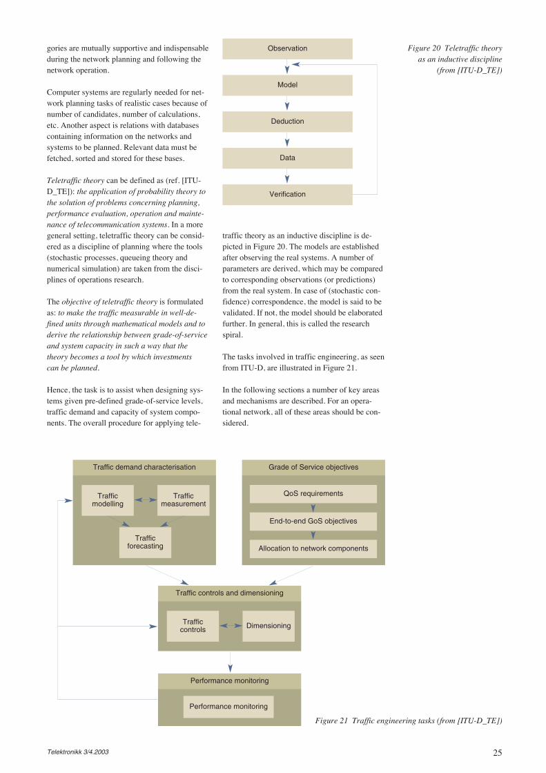
25Telektronikk 3/4.2003
gories are mutually supportive and indispensableduring the network planning and following thenetwork operation.
Computer systems are regularly needed for net-work planning tasks of realistic cases because ofnumber of candidates, number of calculations,etc. Another aspect is relations with databasescontaining information on the networks andsystems to be planned. Relevant data must befetched, sorted and stored for these bases.
Teletraffic theory can be defined as (ref. [ITU-D_TE]): the application of probability theory tothe solution of problems concerning planning,performance evaluation, operation and mainte-nance of telecommunication systems. In a moregeneral setting, teletraffic theory can be consid-ered as a discipline of planning where the tools(stochastic processes, queueing theory andnumerical simulation) are taken from the disci-plines of operations research.
The objective of teletraffic theory is formulatedas: to make the traffic measurable in well-de-fined units through mathematical models and toderive the relationship between grade-of-serviceand system capacity in such a way that thetheory becomes a tool by which investmentscan be planned.
Hence, the task is to assist when designing sys-tems given pre-defined grade-of-service levels,traffic demand and capacity of system compo-nents. The overall procedure for applying tele-
traffic theory as an inductive discipline is de-picted in Figure 20. The models are establishedafter observing the real systems. A number ofparameters are derived, which may be comparedto corresponding observations (or predictions)from the real system. In case of (stochastic con-fidence) correspondence, the model is said to bevalidated. If not, the model should be elaboratedfurther. In general, this is called the researchspiral.
The tasks involved in traffic engineering, as seenfrom ITU-D, are illustrated in Figure 21.
In the following sections a number of key areasand mechanisms are described. For an opera-tional network, all of these areas should be con-sidered.
Observation
Model
Deduction
Data
Verification
Figure 20 Teletraffic theoryas an inductive discipline
(from [ITU-D_TE])
Traffic demand characterisation Grade of Service objectives
Trafficmodelling
Trafficforecasting
Trafficmeasurement
QoS requirements
End-to-end GoS objectives
Allocation to network components
Traffic controls and dimensioning
Trafficcontrols Dimensioning
Performance monitoring
Performance monitoring
Figure 21 Traffic engineering tasks (from [ITU-D_TE])
26 Telektronikk 3/4.2003
where n(t) expresses the (number of) occupiedservers at time t.
Often the unit used for traffic intensity is erlang(referring to the Danish mathematician E.K.Erlang, 1878 – 1929). This unit is actuallydimensionless.
Carried traffic, Ac – The amount of traffic car-ried by the group of servers during a time inter-val. This can be measured by observing theamount of servers being busy in that interval.
The total traffic carried during a time interval isnamed the traffic volume, e.g.
6 Basic Traffic TermsOne commonly meets the term traffic when dis-cussion network planning. Traffic is used todenote traffic intensity; that is, traffic per timeunit. The definition is: Traffic intensity –The instantaneous traffic intensity on a pool ofresources is the number of busy resources ata given instant of time. The pool of resourcesmay be a group of servers. Note that one mayget association of a discrete number of serversalthough the term is generally applicable also fora “continuum” of resources (e.g. for link band-width).
Statistical moment of the traffic intensity can becalculated for a time interval, say from 0 to T,e.g. for the mean value:
That is, Ar = A – Ac = A . (1 – b), where b is theprobability of a request being blocked/rejected.
In the general case, carried traffic is the onlymeasurable dimension (as one does not actuallyknow service times for requests being rejected).
Assuming that a system (pool of servers) hascapacity C, the normalised load is given by
Ac(T ) =1
T
∫T
0
n(t)dt
∫T
0
n(t)dt,
being equal to the sum of all occupation timesinside the time interval. The carried traffic cannever exceed the capacity of the server pool (i.e.a single server unit can never carry more thanone erlang).
Offered traffic, A – The traffic that would be car-ried if no requests were to be rejected due to lackof server capacity. Two types of parameters areoften seen to describe traffic:
• The request intensity, λ, which is the meannumber of requests offered per time unit.
• The mean service time, s, for a request (notethat this must be given with the same time unitas the request intensity).
The offered traffic is then equal to A = λ . s.Again, it is recognized that traffic is dimensionless.
Rejected traffic, Ar – The difference betweenoffered traffic and carried traffic.
ρ =
λ · s
C.
The observed utilisation (i.e. referring to carriedtraffic) is in the interval [0,1].
In a multiservice system different request typesmay occupy different amounts of server unitcapacity. This must be considered when the traf-fic is calculated. Assuming that traffic type ioccupies a server capacity di, the offered trafficfor K request types is found as:
A =
K∑
i=1
λi · si · di
Traffic characterisation is often done by estab-lishing models that approximate the stochasticbehaviour of the traffic flows. As few trafficparameters as possible is strived for (e.g. meanvalue, variance, etc.) while still being able tocapture the pertinent characteristics of the trafficflow. In fact, the key trick in traffic modelling isto identify the simplifying assumptions to bemade and the set of parameters to use.
When possible, measurements are conducted tovalidate the traffic models. On the other hand,measurements could only be done in order toassess the parameter values to be used, for exam-ple when the traffic models as such are fixed orapplied due to previous experience.
For an expected future situation forecasting tech-niques are required in order to estimate the traf-fic demand. A list of ITU-T recommendations inthis area is given in Box A.
Examples of characteristics of the traffic are per-sistence (on-demand or permanent), informationtransfer mode (circuit switched or packetswitched), configuration (point-to-point, multi-point-to-multipoint, etc.), transfer bit rate, QoSparameter requirements, symmetry (unidirec-tional, bi-directional asymmetric, bi-directionalsymmetric), and so forth. These are all related tothe session and connections being parts of thesession.
A session can be initiated according to a process– such as the request initiation process – forexample given by the arrival rate or duration.

27Telektronikk 3/4.2003
Going further into the time scale, phenomenarelating to individual information units (e.g.packets) are considered. These would be packetinterarrival times or packet lengths.
A further dimension is needed for mobile sys-tems where the users’ whereabouts also need tobe considered. That is, the spatial effect has tobe taken into account.
The offered traffic varies as a function of time –in accordance with the activity of the environ-ment of the system considered. For PSTN/ISDNthe term Busy Hour has been defined. Thisrefers to the highest traffic during a day. TheTime Consistent Busy Hour (TCBH) is definedas those 60 minutes (determined with an accu-racy of 15 minutes), which has the highest aver-age traffic over a long period. With this defini-tion it may well happen that the traffic offered inthe busiest hour on some days is higher than thetraffic in the TCBH.
The traffic variations can also be divided intodifferent time scales such as:
• The 24 hours daily variations
• The weekly variations
• The yearly variations; some days or seasonsare expected to have higher traffic such asNew Year’s Eve
• Traffic trends (increases or decreases)
Depending on how the system at hand operates,we may distinguish loss-systems from waiting-time systems. For the former, requests arerejected if all servers are occupied; this is typi-cally the case for calls offered to trunk groups.For waiting-time systems the request is placedinto a queue if it finds the servers occupied uponarrival.
A loss-system has a number of indicators toexpress the level of inadequacy:
• Request congestion: The fraction of requeststhat observes all servers busy upon arrival.
• Time congestion: The fraction of time allservers are busy.
• Traffic congestion: The fraction of the offeredtraffic that is not carried.
Typically, these indicators are used to establishdimensioning standards for server groups.
An inconvenience of waiting-time systems is theresulting waiting time. Not only the mean wait-ing time is of interest, but also the distribution ofthe waiting time. For example some short wait-ing time would barely be noticeable. The rela-tion between the waiting time and the level ofinconvenience for a user is not obvious.
Having finite financial means, it is often notcost-effective to build a system that meets any
Box A – Selected ITU-T Recommendations in the Area ofTraffic Demand Characterisation
Traffic Modelling• E.711 – User demand modelling
• E.712 – User plane traffic modelling
• E.713 – Control plane traffic modelling
• E.716 – User demand modelling in Broadband-ISDN
• E.760 – Terminal mobility traffic modelling
• E.523 – Standard traffic profiles for international traffic streams
Traffic Measurements• E.490 – Traffic measurement and evaluation – general survey
• E.491 – Traffic measurement by destination
• E.500 – Traffic intensity measurement principles
• E.501 – Estimation of traffic offered in the network
• E.502 – Traffic measurement requirements for digital telecommunicationexchanges
• E.503 – Traffic measurement data analysis
• E.504 – Traffic measurement administration
• E.505 – Measurements of the performance of common channel signallingnetwork
• E.743 – Traffic measurements for SS no 7 dimensioning and planning
• E.745 – Cell level measurement requirements for the B-ISDN
Traffic Forecasting• E.506 – Forecasting international traffic
• E.507 – Models for forecasting international traffic
• E.508 – Forecasting new telecommunication services
A-user error Technical errorsand blocking B-user busy
B-user answer Conversation
No answer byB-user
Figure 22 Sequence ofpotential events during a
PSTN set-up
28 Telektronikk 3/4.2003
imaginable situation of request rates. One of theobjectives of teletraffic theory is to find relationsbetween the offered traffic, the system capacityand the resulting service level.
For a loss-system a block-diagram (in severalways similar to the ones used for dependabilityanalyses) can be set up. An example is shown inFigure 22. Such diagrams may also be found forother services, e.g. for accessing a web page/sitewhen browsing, although this service is ratherimplemented by waiting-time servers.
Naturally, the schema depicted in Figure 22 canalso be used to study repeated call attempts. Thatis, the users’ response to unsuccessful requestsimpacts the resulting load on the systems andhence an essential part of dimensioning the system.
One may make a distinction between characteri-sation and modelling, ref. [Macf02]. Characteri-sation refers to a phenomenological descriptionof traffic, i.e. the analyses of measurement data,and the production of high-level statisticaldescriptions. Modelling covers the detailed low-level production of probabilistic models of traf-fic that can actually be used to make predictionsabout network and system behaviour. These twoperspectives come together by the requirementof compatibility – the high-level profile derivedfrom the low-level model must fit the experi-mentally observed characterisation.
On the shorter time scales, traffic descriptors areused as inputs for performance estimation andsystem sizing. A number of usefulness criteriashould be fulfilled for such descriptors [Macf02].Of most basic nature, the descriptors should allowfor mathematically tractable handling and result-ing in useful results. Moreover, they should be:
• Stable – a given stationary traffic flow shouldnot have wildly fluctuating parameters fromone day to another;
• Parsimonious – only a small number ofparameters should be necessary;
• Comprehensible – the significance of theparameters should be easily understood;
• Aggregatable – the parameters of the super-position of two flows should bear a simplerelation to those of its components;
• Scalable – natural growth in traffic should notresult in complex changes in parameters.
7 Controlling Network LoadGeneric requirements on the behaviour of a net-work overload control include:
• Convergence to a state which maximises thethroughput of an overloaded resource subjectto keeping its response times short enough toreduce the occurrence of user abandons.Achieving such convergence automaticallyover a realistic range of overload scenarios(including a range of overloaded resourcecapacitates and number of active trafficsources).
• Minimising ineffective traffic flows by selec-tively throttling flows experiencing high drop-ping ratios.
• Fairness between traffic flows in a certainsense.
Overload situations are typically stimulated bya few events:
• Media-stimulated, e.g. invitations to initiatesessions/accessing pages, casting votes, com-petitions, marketing;
• Emergency situations;
• Network equipment failures, including soft-ware/configuration errors;
• Auto-scheduled session initiations, includingDenial of Service attempts.
In the absence of effective control mechanisms,such overload-triggering events would threatenthe stability of network systems and cause asevere reduction in service levels. Ultimately,systems might fail and the service would not beavailable to users.
End-users are commonly intolerant with respectto long response times to their service requests.Typically, when a user has to wait more than afew seconds, re-attempts are made or the servicerequest is abandoned altogether. Similar phe-nomena are found for different types of services,such as telephone calls, web page accesses andso forth.
User impatience combined with an excessivelylong response time can cause the effectivethroughput of a network resource to collapseto a low level when the original request load ishigh enough. This may come from the resourcespending more of its capacity on partially pro-cessing the requests, not finalising any. Hence, ahuge backlog of requests can occur, while mostof the users’ requests are not being completedbefore a certain threshold is met (the userreleases, re-tries, protocol time-out, etc.).
The user model of this is often assumed to bedescribed by (see Figure 23), i) the persistence
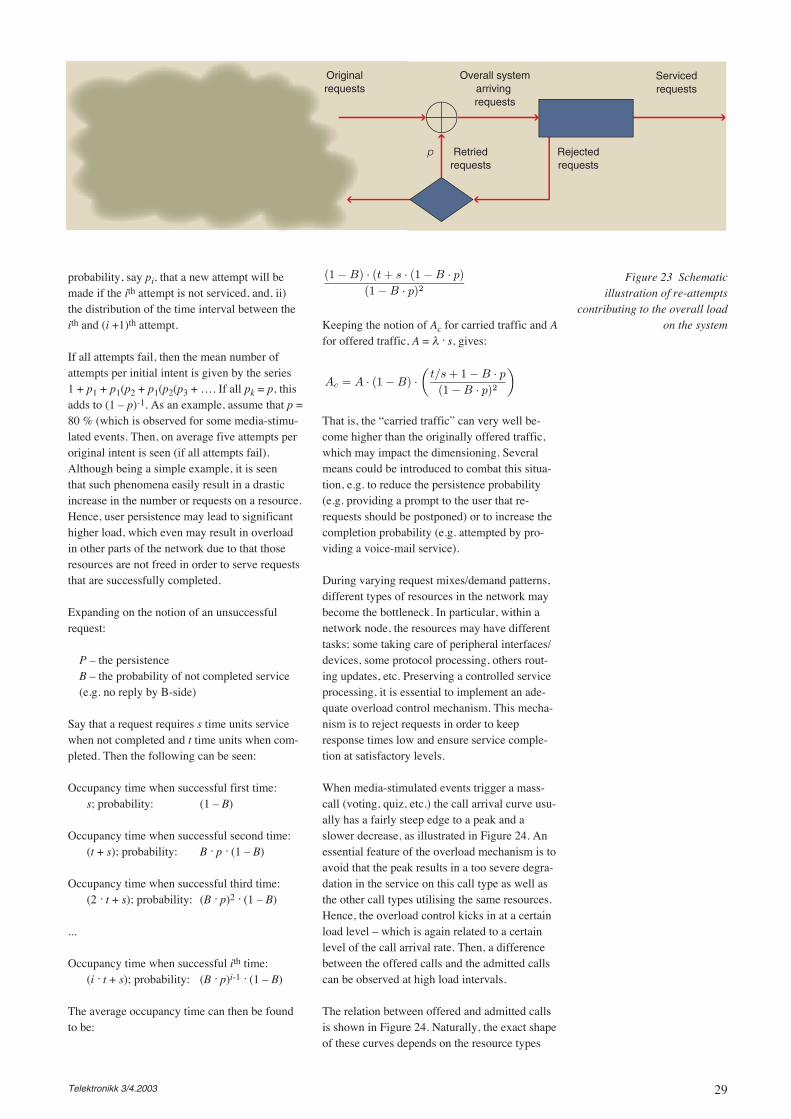
29Telektronikk 3/4.2003
probability, say pi, that a new attempt will bemade if the ith attempt is not serviced, and, ii)the distribution of the time interval between theith and (i +1)th attempt.
If all attempts fail, then the mean number ofattempts per initial intent is given by the series1 + p1 + p1(p2 + p1(p2(p3 + …. If all pk = p, thisadds to (1 – p)-1. As an example, assume that p =80 % (which is observed for some media-stimu-lated events. Then, on average five attempts peroriginal intent is seen (if all attempts fail).Although being a simple example, it is seenthat such phenomena easily result in a drasticincrease in the number or requests on a resource.Hence, user persistence may lead to significanthigher load, which even may result in overloadin other parts of the network due to that thoseresources are not freed in order to serve requeststhat are successfully completed.
Expanding on the notion of an unsuccessfulrequest:
P – the persistenceB – the probability of not completed service(e.g. no reply by B-side)
Say that a request requires s time units servicewhen not completed and t time units when com-pleted. Then the following can be seen:
Occupancy time when successful first time:s; probability: (1 – B)
Occupancy time when successful second time:(t + s); probability: B . p . (1 – B)
Occupancy time when successful third time:(2 . t + s); probability: (B . p)2 . (1 – B)
...
Occupancy time when successful ith time:(i . t + s); probability: (B . p)i-1 . (1 – B)
The average occupancy time can then be foundto be:
Originalrequests
Overall systemarriving requests
Retriedrequests
Rejectedrequests
Servicedrequests
p
Figure 23 Schematicillustration of re-attempts
contributing to the overall loadon the system
(1 − B) · (t + s · (1 − B · p)
(1 − B · p)2
Keeping the notion of Ac for carried traffic and Afor offered traffic, A = λ . s, gives:
Ac = A · (1 − B) ·
(t/s + 1 − B · p
(1 − B · p)2
)
That is, the “carried traffic” can very well be-come higher than the originally offered traffic,which may impact the dimensioning. Severalmeans could be introduced to combat this situa-tion, e.g. to reduce the persistence probability(e.g. providing a prompt to the user that re-requests should be postponed) or to increase thecompletion probability (e.g. attempted by pro-viding a voice-mail service).
During varying request mixes/demand patterns,different types of resources in the network maybecome the bottleneck. In particular, within anetwork node, the resources may have differenttasks; some taking care of peripheral interfaces/devices, some protocol processing, others rout-ing updates, etc. Preserving a controlled serviceprocessing, it is essential to implement an ade-quate overload control mechanism. This mecha-nism is to reject requests in order to keepresponse times low and ensure service comple-tion at satisfactory levels.
When media-stimulated events trigger a mass-call (voting, quiz, etc.) the call arrival curve usu-ally has a fairly steep edge to a peak and aslower decrease, as illustrated in Figure 24. Anessential feature of the overload mechanism is toavoid that the peak results in a too severe degra-dation in the service on this call type as well asthe other call types utilising the same resources.Hence, the overload control kicks in at a certainload level – which is again related to a certainlevel of the call arrival rate. Then, a differencebetween the offered calls and the admitted callscan be observed at high load intervals.
The relation between offered and admitted callsis shown in Figure 24. Naturally, the exact shapeof these curves depends on the resource types
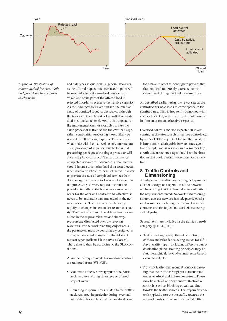
30 Telektronikk 3/4.2003
and call types in question. In general, however,as the offered request rate increases, a point willbe reached where the overload control is in-voked and some part of the offered load isrejected in order to preserve the service capacity.As the load increases even further, the relativeshare of admitted requests decreases, althoughthe trick is to keep the rate of admitted requestsat almost the same level. Again, this depends onthe implementation. For example, in case thesame processor is used to run the overload algo-rithm, some initial processing would likely beneeded for all arriving requests. This is to seewhat to do with them as well as to complete pro-cessing/serving of requests. Due to the initialprocessing per request the single processor willeventually be overloaded. That is, the rate ofcompleted services will decrease, although thisshould happen at a higher load than would occurwhen no overload control was activated. In orderto prevent the rate of completed services fromdecreasing, the load control – as well as any ini-tial processing of every request – should beplaced externally to the bottleneck resource. Inorder for the overload control to be effective, itneeds to be automatic and embedded in the net-work resource. This is to react sufficientlyrapidly to changes in demand or resource capac-ity. The mechanism must be able to handle vari-ations in the request mixtures and the wayrequests are distributed over the relevantresources. For network planning objectives, allthe parameters must be coordinately assigned incorrespondence with targets for the differentrequest types (reflected into service classes).These should then be according to the SLA con-ditions.
A number of requirements for overload controlsare (adopted from [Whit02]):
• Maximise effective throughput of the bottle-neck resource, during all ranges of offeredrequest rates.
• Bounding response times related to the bottle-neck resource, in particular during overloadintervals. This implies that the overload con-
trols have to react fast enough to prevent thatthe total load too greatly exceeds the pro-cessed load during the load increase phase.
As described earlier, using the reject rate as thecontrolled variable leads to convergence in theadmitted rate. This is frequently combined witha leaky bucket algorithm due to its fairly simpleimplementation and effective response.
Overload controls are also expected in severalcoming applications, such as service control, e.g.by SIP or HTTP requests. On the other hand, itis important to distinguish between messages.For example, messages releasing resources (e.g.circuit disconnect message) should not be throt-tled as that could further worsen the load situa-tion.
8 Traffic Controls andDimensioning
An objective of traffic engineering is to provideefficient design and operation of the networkwhile assuring that the demand is served withinthe requirements stated. Network dimensioningassures that the network has adequately config-ured resources, including the physical networkelements and the logical network elements (e.g.virtual paths).
Several items are included in the traffic controlscategory ([ITU-D_TE]):
• Traffic routing: giving the set of routingchoices and rules for selecting routes for dif-ferent traffic types (including different source-destination pairs). Routing principles may beflat, hierarchical, fixed, dynamic, state-based,event-based, etc.
• Network traffic management controls: ensur-ing that the traffic throughput is maintainedunder overload and failure conditions. Thesemay be restrictive or expansive. Restrictivecontrols, such as blocking or call gapping,throttle the traffic sources. The expansive con-trols typically reroute the traffic towards thenetwork portions that are less loaded. Often,
Capacity
Load Serviced load
Rejected loadLoad control
activated
Gaia by activityload control
Load controlactivated
Time Offeredload
Figure 24 Illustration ofrequest arrival for mass-callsand gains from load controlmechanisms
31Telektronikk 3/4.2003
real-time monitoring of the performance/loadlevels triggers these actions related to pre-defined levels. For example, when the numberof calls on a link is equal to a given threshold,additional calls are rejected.
• Service protection methods: controlling thegrade of service of certain traffic types by util-ising discriminatory restriction of access toresource groups.
One example is to balance GoS between traffictypes requesting bandwidth. Another example isto provide stability in networks without hierar-chical routing schemes by restricting overflowtraffic to an alternative route that is shared withfirsts-choice traffic.
When several traffic types compete for the net-work resources, the requirements of the individ-ual types have to be checked to ensure that theirservice levels should be met. Several systemssupport prioritisation of traffic, including sepa-rate criteria for admission control, schedulingand dropping rules.
Designing systems that continue to operate atmaximum capacity even during overloads, vari-ous overload strategies can be introduced. Forprocessing and signalling tasks leaky bucket,gapping and level priorities are seen. For infor-mation transfer modes, bandwidth reservationand circuit channels protection can be used,besides various routing separations.
Bandwidth reservations can for example be usedin hierarchical networks with alternative routingwhere the primary traffic could be protectedagainst load from overflow traffic (overflowtraffic refers to flows that are rerouted onto sec-ondary choices, e.g. when the primary route iscongested). A common rule is that overflow traf-fic is only accepted if more than a given band-width is available.
Virtual channel protection includes two schemes;i) each traffic type is allocated a minimum band-width ensuring a minimum service level, and, ii)a maximum allocation per traffic type avoidingthat a single traffic type dominates.
Packet-level traffic controls assure the packet-level GoS objectives under any network condi-tion and that a cost-efficient GoS differentiationis made between services with different packet-level QoS requirements. A selection of ITU-Trecommendations for traffic controls and dimen-sioning is listed in Box B.
In some respects, an incorrectly dimensionednetwork will have a degraded performance levelin a similar manner as a network experiencing
failures. Hence, dependability analyses and traf-fic analyses should be considered together. Fordependability analyses the phenomenon that afault may appear might be modelled as a processwith given distributions, as well as the repairtime of the failure. A fairly simple model of asystem is expressed by a block diagram, whereall essential components are reflected. Then,series and parallel branches are resolved to esti-mate the overall system dependability.
A growing part of telecom systems is made ofsoftware modules in different nodes interacting.Considering replication of data and program rou-tines, a certain level of dependency may be pre-sent although from a (hardware) point of viewthe resources are completed. It is vital to con-sider the commonalities and dependencies in adependability model to avoid that incorrect con-clusions are drawn.
In one way, technical risk analyses are related tothe dependability. Then the risk can be definedas the product of the probability and the conse-quence of an event. The overall risk becomes thesum over all the events. In several cases, quanti-tative estimates of the events are challenging toestimate, resulting in risk diagrams having con-sequence and probability on the axes – cate-
Box B – Selected ITU-T Recommendations for TrafficControls and Dimensioning
Circuit-switched Networks• E.510 – Determination of the number of circuits in manual operation
• E.520 – Number of circuits to be provided in automatic and/or semi-automaticoperation, without overflow facilities
• E.521 – Calculations of the number of circuits in a group carrying overflowtraffic
• E.522 – Number of circuits in a high-usage group
• E.524 – Overflow approximations for non-random inputs
• E.525 – Designing network to control grade of service
• E.526 – Dimensioning a circuit group with multi-slot bearer services and nonoverflow inputs
• E.527 – Dimensioning a circuit group with multi-slot bearer services andoverflow traffic
• E.528 – Dimensioning of digital circuit multiplication equipment (DCME)systems
• E.529 – Network dimensioning using end-to-end GoS objectives
• E.731 – Methods for dimensioning resources operating in circuit switched mode
Broadband Integrated Services Digital Network• E.735 – Framework for traffic control and dimensioning in B-ISDN
• E.736 – Methods for cell level traffic control in B-ISDN
• E.737 – Dimensioning methods for B-ISDN
Signalling and Service Control• E.733 – Methods for dimensioning resources in Signalling System no. 7
networks
• E.734 – Methods for allocating and dimensioning Intelligent Network (IN)resources
32 Telektronikk 3/4.2003
one may say that a future standpoint is takenlooking back towards today to reveal thecauses of that scenario to appear. A character-istic of Delphi and expert panels is that severalrounds are carried out, where the participantsmay get feedback on the statements of othersin between. This is to try to achieve a conver-gence on opinions.
Traffic forecasting is necessary both for strategicstudies as well as when designing systems on amedium term. Broadly, two basic approachesmight be identified for forecasting:
• Descriptive approach, where the basicassumption is that the underlying process gen-erating the demand in the past continues intothe future. Statistical model is for exampleapplicable in this case, whereby the timeseries (or demand history) is analysed forcomponents such as the base or constant com-ponent, trends, etc. Then, this description isextrapolated into the future. Naturally, knowl-edge of any impending events should beincluded in the extrapolation.
• Explanatory approach, where casual relation-ships are built into the model. Several modelscan be found in the literature, such as wideeconometric models to models predicting thepurchasing patterns for a group of customers.
For all the forecasting a random error compo-nent (sometimes referred to as noise) is present.This composes the unexplained deviation of thedata from the basic demand generating process.
When returning to the descriptive models, thefollowing patterns are commonly consideredwhen relevant, see Figure 25:
• Base – representing a central tendency of thetime series at any given time
• Trend – exhibiting a consistent long-run shiftof the average
• Seasonal – showing a repetitive variation, e.g.a one-year periodicity. This is commonlysuperposed upon a background process, e.g.showing a trend.
As time passes, new information is gained andthe models can be updated. When doing thiseither the time origin can be fixed or the timeorigin can be shifted to the end of the currentperiod. In the former, the parameters have to berecomputed every time in order to incorporatethe latest observations. In the latter, also calledadaptive smoothing, the parameters are updatedby combining the old estimates and the latestforecast error recorded.
gorised by small, medium and high. The riskprofile of a company then decides which mea-sures to apply trying to eliminate the events thatare most unwanted.
A part of the network planning area is to formu-late contingency plans. These may be expressedas; what to do when XX happens. Then, respon-sible units and their actions have to be clear tothe parties involved. Moreover, all XX eventsshould be captured. Examples of events are firein a station, major vehicle accidents involvingpolice, ambulance, etc.
9 ForecastingConsidering the steadily changing environmentof a telecom actor, it is essential to have ideas onwhat the future situation will be like. In particu-lar this is relevant for the demand patterns. Vari-ous forecasting techniques are applied to get anobjective view of the future situation – this iscommonly done by looking at the forces work-ing in the past, present and future periods.
Two basically different approaches for makingforecasts are:
• Quantitative – including trend and factor meth-ods, analogy methods and potentials. A trend isa statistical description of a historic and rele-vant development that is prolonged into thefuture. A basic precondition for doing this isthat factors that influence the developmenthave been examined and their potentiallychanging magnitudes in the future captured inthe predictions. An analogy method can beapplied when the case at hand is believed to fol-low a similar evolution as another known case(e.g. another region/nation, another product,another customer segment, etc.). This methodmay also be applied when relating productswith other industries. A potential for a productor customer segment (also referred to as satura-tion level) could possible be transferred fromother industries or other product groups. Forexample, the number of internet subscriptionswill not likely exceed the number of PCs.
• Qualitative – including perspective and sce-nario analyses, and interviews and question-naires (such as Delphi and expert panels). Theperspective method aims at describing likelydevelopment tracks commonly based on dis-cussions on technological, market, social andeconomic evolution in the period. Hence, thiswill take today’s standpoint and derive thepotential future based on that view. In a sce-nario method a more or less remote future istaken on. Potential alternative futures – sce-narios – are then elaborated, possibly withoutdescribing what happened between today andthat point in the future. Hence, for a scenario
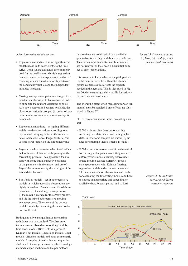
33Telektronikk 3/4.2003
In case there are no historical data available,qualitative forecasting models are most relevant.Time series models and Kalman filter modelsare not relevant as they need a substantial num-ber of (pre-)observations.
It is essential to know whether the peak periodsfor different services for different customergroups coincide as this affects the capacityneeded in the network. This is illustrated in Fig-ure 26, demonstrating a daily profile for residen-tial and business customers.
The averaging effect when measuring for a giveninterval must be handled. Some effects are illus-trated in Figure 27.
ITU-T recommendations in the forecasting areaare:
• E.506 – giving directions on forecastingincluding base data, social and demographicdata. In case some samples are missing, guid-ance for obtaining these elements is found.
• E.507 – presents an overview of mathematicalforecasting techniques: curve-fitting models,autoregressive models, autoregressive inte-grated moving average (ARIMA) models,state space models with Kalman filtering,regression models and econometric models.This recommendation also contains methodsfor evaluating the forecasting models and howto choose an appropriate one depending onavailable data, forecast period, and so forth.
A few forecasting techniques are:
• Regression methods – fit some hypothesizedmodel, linear in its coefficients, to the timeseries. Least square estimators are commonlyused for the coefficients. Multiple regressioncan also be used as an explanatory method ofrecasting when a causal relationship betweenthe dependent variables and the independentvariables is present.
• Moving average – computes an average of theconstant number of past observations in orderto eliminate the random variations or noise.As a new observation becomes available, theoldest observation is dropped (in order to keeptheir number constant) and a new average iscomputed.
• Exponential smoothing – assigning differentweights to the observations according to anexponential decaying factor as the time dis-tance increases. Hence, longer (historic) val-ues get lower impact on the forecasted value.
• Bayesian methods – useful when faced with alack of historical data at the beginning of theforecasting process. The approach is then tostart with some initial subjective estimateof the parameters in the model, and use ofBayes’ theorem to modify them in light of theactual data observed.
• Box-Jenkins models – set of autoregressivemodels in which successive observations arehighly dependent. Three classes of models areconsidered; i) the autoregressive process,ii) the moving average (or the errors) process,and iii) the mixed autoregressive-movingaverage process. The choice of the correctmodel is made by examining the autocorrela-tion coefficients.
Both quantitative and qualitative forecastingtechniques can be exercised. The first groupincludes models based on smoothing models,time series models (Box Jenkins approach),Kalman filter models, Regression models, Logitmodels, diffusion models and other econometricmodels. Examples of qualitative techniques in-clude market surveys, scenario methods, analogymethods, expert methods and Delphi methods.
(a) (b) (c)
Demand Demand Demand
Time Time Time
Figure 25 Demand patterns:(a) base, (b) trend, (c) trend
and seasonal variations
Sum of business and residential
Residential
Business
Integration gain
Time-of-day
Traffic load
1
2 4 6 8 10 12 14 16 18 20 22 24
2
3
4
5 Sum of max (business) and max (residential)
Figure 26 Daily trafficprofiles for different
customer segments
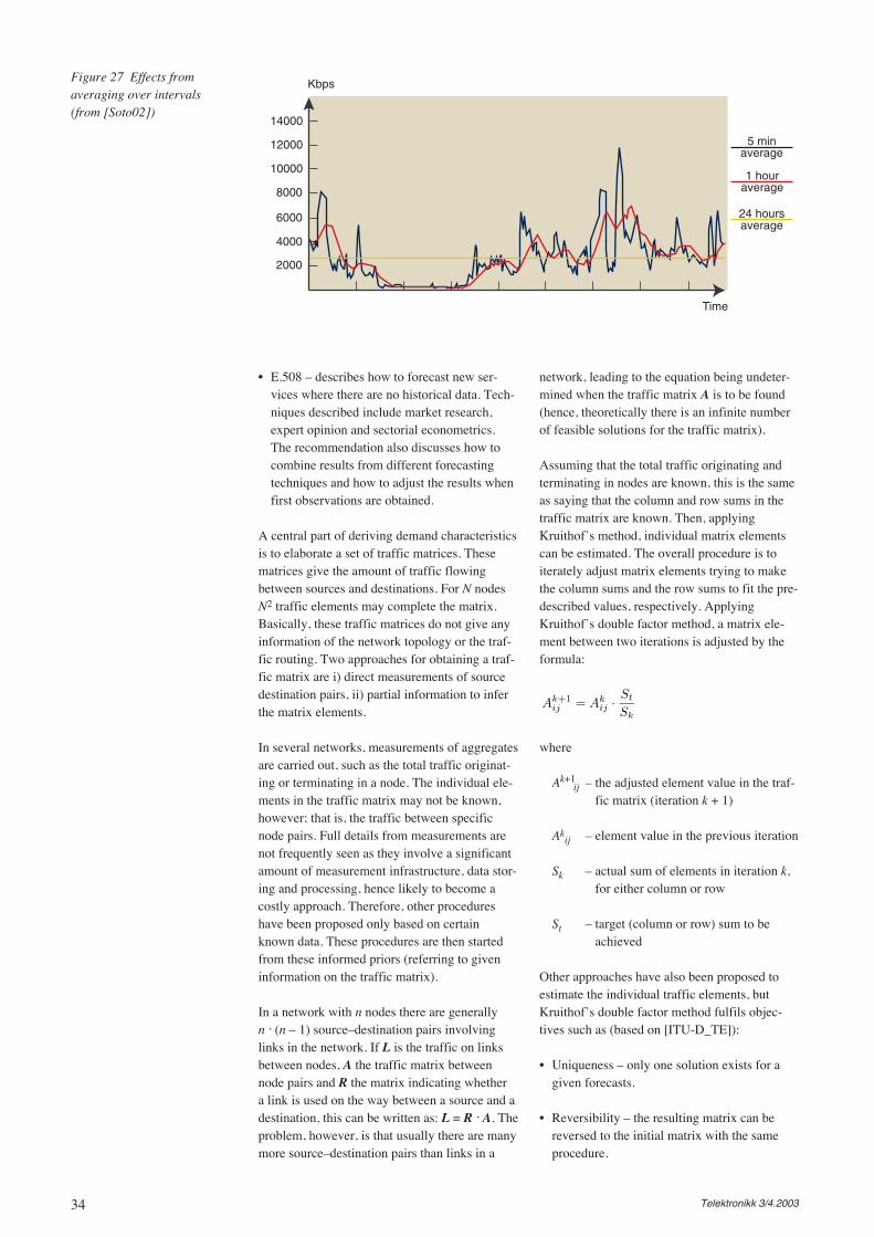
34 Telektronikk 3/4.2003
• E.508 – describes how to forecast new ser-vices where there are no historical data. Tech-niques described include market research,expert opinion and sectorial econometrics.The recommendation also discusses how tocombine results from different forecastingtechniques and how to adjust the results whenfirst observations are obtained.
A central part of deriving demand characteristicsis to elaborate a set of traffic matrices. Thesematrices give the amount of traffic flowingbetween sources and destinations. For N nodesN2 traffic elements may complete the matrix.Basically, these traffic matrices do not give anyinformation of the network topology or the traf-fic routing. Two approaches for obtaining a traf-fic matrix are i) direct measurements of sourcedestination pairs, ii) partial information to inferthe matrix elements.
In several networks, measurements of aggregatesare carried out, such as the total traffic originat-ing or terminating in a node. The individual ele-ments in the traffic matrix may not be known,however; that is, the traffic between specificnode pairs. Full details from measurements arenot frequently seen as they involve a significantamount of measurement infrastructure, data stor-ing and processing, hence likely to become acostly approach. Therefore, other procedureshave been proposed only based on certainknown data. These procedures are then startedfrom these informed priors (referring to giveninformation on the traffic matrix).
In a network with n nodes there are generallyn . (n – 1) source–destination pairs involvinglinks in the network. If L is the traffic on linksbetween nodes, A the traffic matrix betweennode pairs and R the matrix indicating whethera link is used on the way between a source and adestination, this can be written as: L = R . A. Theproblem, however, is that usually there are manymore source–destination pairs than links in a
network, leading to the equation being undeter-mined when the traffic matrix A is to be found(hence, theoretically there is an infinite numberof feasible solutions for the traffic matrix).
Assuming that the total traffic originating andterminating in nodes are known, this is the sameas saying that the column and row sums in thetraffic matrix are known. Then, applyingKruithof’s method, individual matrix elementscan be estimated. The overall procedure is toiterately adjust matrix elements trying to makethe column sums and the row sums to fit the pre-described values, respectively. ApplyingKruithof’s double factor method, a matrix ele-ment between two iterations is adjusted by theformula:
Time
5 minaverage
1 houraverage
24 hoursaverage
Kbps
2000
4000
6000
8000
10000
12000
14000
Figure 27 Effects fromaveraging over intervals (from [Soto02])
Ak+1
ij = Akij ·
St
Sk
where
Ak+1ij – the adjusted element value in the traf-
fic matrix (iteration k + 1)
Akij – element value in the previous iteration
Sk – actual sum of elements in iteration k,for either column or row
St – target (column or row) sum to beachieved
Other approaches have also been proposed toestimate the individual traffic elements, butKruithof’s double factor method fulfils objec-tives such as (based on [ITU-D_TE]):
• Uniqueness – only one solution exists for agiven forecasts.
• Reversibility – the resulting matrix can bereversed to the initial matrix with the sameprocedure.
35Telektronikk 3/4.2003
• Transitivity – the resulting matrix is the sameindependent of whether it is obtained in onestep or via a series of intermediate transforma-tions.
• Invariance – regarding the sequence of nodes;their sequence may be changed without influ-encing the results.
• Fractioning – the individual nodes can be splitinto sub-nodes or be aggregated into largernodes without influencing the result. Note thatthis is not completely met for Kruithof’s dou-ble factor method, but deviations are small.
10 Performance Objectivesand Service Constraints
Grade of Service (GoS) is defined as a numberof traffic engineering parameters to provide ameasure of adequacy of plant under specifiedconditions. GoS parameters are expressed asprobability of blocking delay distribution, etc.Network Performance (NP) is defined as theability of a network or network portion to pro-vide the functions related to communicationsbetween users. GoS is the traffic-related part ofNP, although NP also covers non-traffic relatedaspects (including dependability, charging, etc.).
NP and GoS objectives are derived from Qualityof Service requirements. Basically, QoS shouldbe user-oriented and, in principle, independentof the network. NP parameters though, are net-work-oriented; i.e. they can be used when speci-fying performance requirements.
A common approach followed so far by ITU-Tis to define a so-called reference connection inorder to derive GoS conditions for a networkportion. Then, an end-to-end connection is parti-tioned into portions and the QoS requirementsare divided into contributions from each of theportions. In several cases, an interface betweentwo portions refers to an interface between twooperators/providers. A number of recommenda-tions address reference connections, including:
• E.701 – Reference connections for trafficengineering
• E.751 – Reference connections for trafficengineering of land mobile networks
• E.752 – Reference connections for trafficengineering of maritime and aeronauticalsystems
• E.755 – Reference connections for UPT trafficperformance and GoS
• E.651 – Reference connections for trafficengineering of IP access networks
As described above, defining the reference con-nection is followed by elaborating GoS objec-tives. A number of recommendations are foundfor this purpose too:
• E.540 – Overall grade of service of the inter-national pert of an international connection
• E.541 – Overall grade of service for interna-tional connections (subscriber-to-subscriber)
• E.543 – Grades of service in digital interna-tional telephone exchanges
• E.550 – Grade of service and new perfor-mance criteria under failure conditions ininternational telephone exchanges
• E.720 – ISDN grade of service concept
• E.721 – Network grade of service parametersand target values for circuit-switched servicesin the evolving ISDN
• E.723 – Grade-of-service parameters forSignalling System No. 7 networks
• E.724 – GoS parameters and target GoSobjectives for IN Services
• E.726 – Network grade of service parametersand target values for B-ISDN
• E.728 – Grade of service parameters forB-ISDN signalling
• E.770 – Land mobile and fixed network inter-connection traffic grade of service concept
• E.771 – Network grade of service parametersand target values for circuit-switched landmobile services
• E.773 – Maritime and aeronautical mobilegrade of service concept
• E.774 – Network grade of service parametersand target values for maritime and aeronauti-cal mobile services
• E.775 – UPT Grade of service concept
• E.776 – Network grade of service parametersfor UPT
• E.671 – Post selection delay for PSTN/ISDNsusing Internet telephony for a portion of theconnection
• E.651 – Reference connections for trafficengineering of IP access networks
36 Telektronikk 3/4.2003
• Y.1540 – Internet protocol data communica-tion service – IP packet transfer and availabil-ity performance parameters
• Y.1541 – Network performance objectives forIP-based services
Looking into these one finds a separationbetween the user data performance and sig-nalling performance. Examples of parameters ofthe former are information transfer delay, infor-mation delay variation, information loss ratio,etc. Examples of the latter are set-up delay, dis-connection delay, connection set-up blocking,etc. In most cases the GoS requirements referto a fully operational network, not taking intoaccount network failures. One exception isE.550 which combines the effect of availabilityand traffic congestion and defines parametersand target values that consider their joint effect.
11 Performance TestingPerformance testing belongs to the non-func-tional verification of a system operation. That is,not the does the system deliver a proper result(being a functional examination), but rather howdoes the system deliver a proper result. Theremay be several goals for carrying out perfor-mance testing, including:
• Identify bottlenecks and determine configura-tion for maximal performance
• Determine capacity of a system and effectsunder overload
• Examine effects of introducing additionalmodules, new releases, etc.
One advantage by performance testing is that itcould work on the final system, avoiding testingon models which might – or might not – fullyreflect the behaviour of the system. However,this is also a drawback as a complete testing thenmust be delayed until the system is fully config-ured – coming rather late in the developmentcycle. Moreover, the testing may become moreexpensive compared to testing on a model. Thismay also come in addition to real traffic beingoffered to the system, potentially impacting thecustomer. Due to the steady pressure on releas-ing new systems/products, vendors often choosenot to conduct full testing, but rather restrict theexaminations to so-called representative tests.However, these tests may not fully cover theoperational situation the system might experi-ence.
Performance modelling is the abstraction of areal system into a simplified representation toenable the prediction of performance. Note,however, that this term commonly means differ-
ent things to different people. When new sys-tems are to be introduced the components’capacity should be known. This can be obtainedby measuring, under controlled conditions, or bymodelling the components before the system isdeployed. This allows for a more accurate di-mensioning and provides a basis for followingthe performance during operation.
Performance and traffic analyses should be car-ried out for several phases of a system life,including:
• Design – the design principles may be studiedto find which ones to choose
• Delivery – the specifications are to be verifiedby the receiver of a system
• Operation – performance under varying condi-tions, also when the system is enhanced ormodified in other ways.
When an actual system is to be modelled, theamount of technical specification and data to becaptured may be overwhelming, although moreintriguing to concisely formulate in a model. Inprinciple, a balance between the completeness ofthe model and its tractability can be faced. Thismakes the art of system modelling even morepleasing.
One goal of including performance engineeringat all stages of the product life-cycle is to pre-vent problems. This also applies to systems inoperation. Measuring during operation also givesadditional insight as successful services tend togrow whereas unsuccessful ones usually shrink.Monitoring, comparing results to forecasts andthe capacity can give early warnings of any sys-tem enhancements to be planned. Depending onthe lead-time for enhancements this can be cru-cial during operation.
Detecting faults is also a result of performanceengineering. Fault-tolerant systems, distributedsystems and data inconsistence etc. may lead todegradation only, which could be detected withperformance testing – possibly assisted by trac-ing capabilities.
In one way, when a system’s data and process-ing become more distributed, the performancerisk does as well. Rapid development and auto-generation of program code may also add to theperformance risk. This underlines the need forperformance engineering, in particular the per-formance prediction using adequate tools andmodels. The following benefits of performancemodelling are listed in [Sing02]:
37Telektronikk 3/4.2003
• Relatively inexpensive prediction of futureperformance
• Design support allowing objective choices tobe made
• Decision support for further development ofexisting systems
• A clearer understanding of a system’s perfor-mance characteristics
• A mechanism for risk management and reduc-tion.
Relations with different phases of the systemdevelopment are illustrated in Figure 28.
For analytic treatment, simulation and measure-ments several common aspects are seen, includ-ing ([Sing02]):
I Model requirements – what questions are tobe answered by the model
II System understanding – gathering all theperformance characteristics of the system orprocess
III Model design and development – translatingthe system design into a model design, deter-mining what to include and to exclude
IV Data collection – usually takes the most(elapsed) time and should be started as soonas possible, e.g. low-level system data notreadily available, such as the number of CPUseconds taken by a process to perform a par-ticular task
V Model verification – ensuring the modeldesign reflects the system design by testingthe model at various levels and model walk-throughs in conjunction with the systemdesigners, developers and users
VI Model validation – if possible running themodel to reflect the real system using the sameinput and checking the similarity of the output“what if” scenarios, predictions and answers tothe questions – exercising the model withspecific inputs designed to answer the ques-tions defined in the model r equirements
Iterations are often done for several of the stagesin the process, e.g. as requirements are changed,a greater understanding gained and improveddata quality of data is gathered. Simpler modelscan be produced early to give an initial predic-tion. As time evolves more design informationand input data are available, models could berefined and accuracy gained.
12 Measurements andMonitoring
Basically, measurements are carried out in orderto obtain quantitative estimates about the systembehaviour, traffic characteristics, performancelevels and so forth. A number of objectives ofmeasuring can be identified, including estimat-ing performance, characterising traffic flows,charging inputs, documenting SLA conditions,and so forth. Hence, different measurementschemes have been defined. Although a networkmay be correctly dimensioned, overload andfailure situations are likely to occur where net-work traffic management actions have to be ini-tiated. Moreover forecast errors or approxima-tions, statistical variations in the demand, alsolead to degraded service levels. GoS monitoringis needed to detect these problems and providefeedback for network design and traffic charac-terisation. Depending on the problems faced,network re-configuration, changes in routingpatters, adjustment in traffic control parametersor network extensions may be initiated.
In ITU-T a number of recommendations arefound relating to measurements and monitoring;a short list follows:
• E.490 – Introduction to the series on trafficand performance measurements, includinga survey and application of results for shortterm (input to network management actions),medium term (inputs to maintenance andreconfiguration), and long term (foundationsfor network extensions).
• E.491 – Application of traffic measurementsby destination for network planning, describ-ing the approaches of call detail recording anddirect measurements.
• E.492 – Traffic reference period
• E.493 – Grade of Service (GoS) monitoring
• E.504 – Describing operation procedures formeasurements (by human operators and byunderlying system).
• E.503 – Potential applications of the measure-ments and operational procedures for obtain-ing the analysis results.
• E.500 – Describing the principles for trafficintensity measurements, including a generali-sation of the busy interval approach. Termslike estimates for daily peak traffic intensity,normal load and high load for month and yearare introduced.
• E.501 – Describing methods for estimatingoffered traffic to a resource group and the ori-
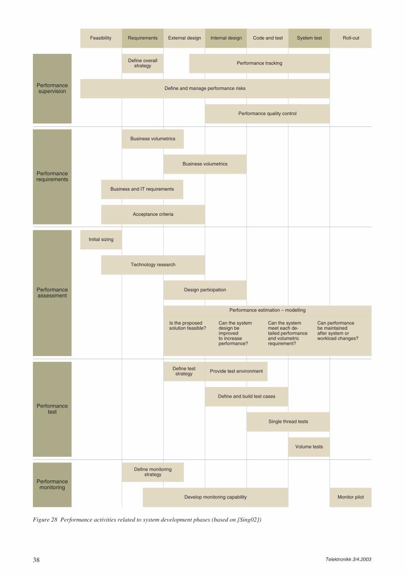
38 Telektronikk 3/4.2003
Roll-outSystem testCode and testInternal designExternal designFeasibility Requirements
Define overallstrategy
Business volumetrics
Initial sizing
Technology research
Design participation
Define teststrategy
Define monitoringstrategy
Monitor pilotDevelop monitoring capability
Provide test environment
Define and build test cases
Single thread tests
Volume tests
Is the proposed Can the system Can the system Can performancesolution feasible? design be meet each de- be maintained
improved tailed performance after system orto increase and volumetric workload changes?performance? requirement?
Performance estimation – modelling
Business volumetrics
Business and IT requirements
Acceptance criteria
Performance tracking
Define and manage performance risks
Performance quality control
Performancesupervision
Performancerequirements
Performanceassessment
Performancetest
Performancemonitoring
Figure 28 Performance activities related to system development phases (based on [Sing02])
39Telektronikk 3/4.2003
gin-destination traffic demand based on mea-surements on a circuit group.
• E.502, E.505, E.745 – Specifies traffic andperformance measurement requirements forPSND/SIDN, common signalling system no.7 networks, B-ISDN exchanges, respectively
• E.743 – Identifies the subset of measurements(of E.505) to be used for dimensioning andplanning of common signalling system no. 7networks.
The type of measurements and parameters to beestimated must be in accordance with the objec-tive of the measurements. Defining the measure-ment procedure implies balancing the technicaland administrative efforts against informationgained. According to the stochastic nature oftraffic, a time limited measurement gives obser-vation of certain realisation of the traffic pro-cess. Thus, this can be seen as a sample of theunderlying traffic process. Repeating the mea-suring one often sees different values. Therefore,one can commonly only state statistical mea-sures of the traffic process, e.g. a mean value,variation. Having full information of the trafficprocess implies that the distribution function isknown.
A traffic process that is discrete in state and con-tinuous in time can, in principle, be measured bycombining:
• Measurements of number of events, e.g. num-ber of requests, number of errors.
• Measurements of time intervals, e.g. process-ing times, session times, waiting times.
Two broad categories of measurement methodsare; i) continuous measurements, and, ii) discretemeasurements. Another categorisation is, i) pas-sive measurements, and ii) active measurements.In the latter case test traffic is typically injectedinto the system, possibly influencing the result-ing system behaviour and performance and fac-ing the challenge of defining patterns of the testtraffic for it to mimic the process that is to beestimated.
A general challenge for sampling, including bothmeasurements and simulations, is to derive anestimate of the level of confidence that should beplaced on the values estimated. Let us assumethat we have N independent and identically dis-tributed observations {X1, X2, …, XN} of a ran-dom variable with unknown finite mean value mand finite variance σ2.
The mean and variance of the sample are definedas:
Both and s2 are functions of a random vari-able and hence, random variables themselves,defined by a distribution called the sample distri-bution. The first is the main estimator for thepopulation mean value;
X =1
N·
N∑i=1
Xi, s2
=1
N − 1·
[N∑
i=1
X2
i− N · X2
].
E[X] = m
σ2
[X
]=
s2
N
X ± tN−1,(1−α/2) ·
√s2
N,
X
s2/N is an estimator of the variance of the samplemean, , that is:X
The accuracy of an estimate of a sample parame-ter is described by the confidence interval. Theconfidence interval specifies how the estimateis placed relatively to the unknown theoreticalvalue with a given probability. Given theassumptions above, this confidence interval ofthe mean value becomes:
where tN-1, (1-α/2) is the upper (1 – α/2) per-centile of the t-distribution with N – 1 degrees offreedom. (1 – α) is called the level of confidenceand expresses the probability that the confidenceinterval includes the unknown theoretical meanvalue. When N becomes larger the t-distributionconverges to a Normal distribution.
Note the assumption of independence of thesampling events. This assumption might be bro-ken if the observations are made too close as thevalues then can be correlated. Similar for simu-lations, different starting seeds should be appliedto strive for independence of the simulationtraces.
13 Traffic HandlingMechanisms
Three main groups of traffic handling mecha-nisms are:
• Classification: At the ingress, the traffic isclassified on a packet-by packet basis into oneof the defined service classes. Typically anapplication may be looked for by means ofstatic field information, e.g. in the packetheaders.
• Traffic conditioning (policing and marking):Commonly some form of policing to some orall of the defined service classes, to ensurethat usage remains within prescribed levels.This is particularly vital for the more appreci-ated classes, which should often receive bettertreatment, and thereby result in higher cost tothe network operator. Policing refers to decid-
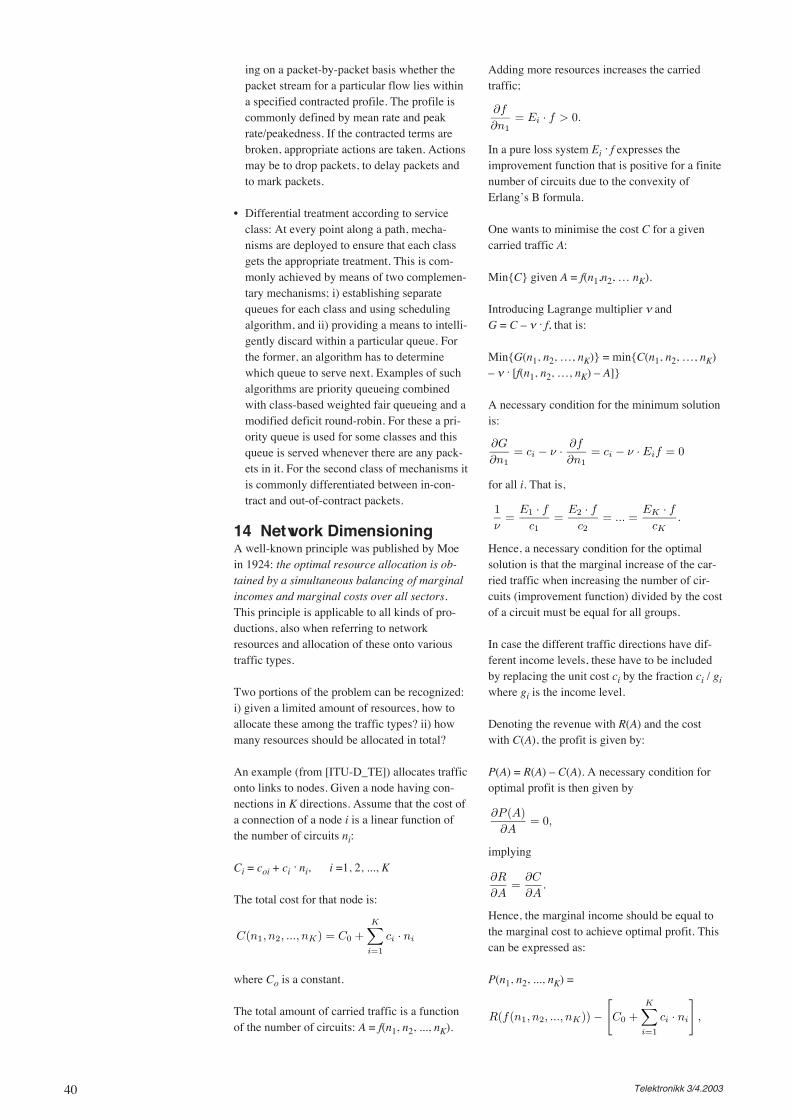
40 Telektronikk 3/4.2003
Hence, a necessary condition for the optimalsolution is that the marginal increase of the car-ried traffic when increasing the number of cir-cuits (improvement function) divided by the costof a circuit must be equal for all groups.
In case the different traffic directions have dif-ferent income levels, these have to be includedby replacing the unit cost ci by the fraction ci / gi
where gi is the income level.
Denoting the revenue with R(A) and the costwith C(A), the profit is given by:
P(A) = R(A) – C(A). A necessary condition foroptimal profit is then given by
ing on a packet-by-packet basis whether thepacket stream for a particular flow lies withina specified contracted profile. The profile iscommonly defined by mean rate and peakrate/peakedness. If the contracted terms arebroken, appropriate actions are taken. Actionsmay be to drop packets, to delay packets andto mark packets.
• Differential treatment according to serviceclass: At every point along a path, mecha-nisms are deployed to ensure that each classgets the appropriate treatment. This is com-monly achieved by means of two complemen-tary mechanisms; i) establishing separatequeues for each class and using schedulingalgorithm, and ii) providing a means to intelli-gently discard within a particular queue. Forthe former, an algorithm has to determinewhich queue to serve next. Examples of suchalgorithms are priority queueing combinedwith class-based weighted fair queueing and amodified deficit round-robin. For these a pri-ority queue is used for some classes and thisqueue is served whenever there are any pack-ets in it. For the second class of mechanisms itis commonly differentiated between in-con-tract and out-of-contract packets.
14 Network DimensioningA well-known principle was published by Moein 1924: the optimal resource allocation is ob-tained by a simultaneous balancing of marginalincomes and marginal costs over all sectors.This principle is applicable to all kinds of pro-ductions, also when referring to networkresources and allocation of these onto varioustraffic types.
Two portions of the problem can be recognized:i) given a limited amount of resources, how toallocate these among the traffic types? ii) howmany resources should be allocated in total?
An example (from [ITU-D_TE]) allocates trafficonto links to nodes. Given a node having con-nections in K directions. Assume that the cost ofa connection of a node i is a linear function ofthe number of circuits ni:
Ci = coi + ci. ni, i =1, 2, ..., K
The total cost for that node is:
Adding more resources increases the carriedtraffic;
C(n1, n2, ..., nK) = C0 +K∑
i=1
ci · ni
∂f
∂n1
= Ei · f > 0.
∂G
∂n1
= ci − ν ·
∂f
∂n1
= ci − ν · Eif = 0
1
ν=
E1 · f
c1
=E2 · f
c2
= ... =EK · f
cK
.
∂P (A)
∂A= 0,
∂R
∂A=
∂C
∂A.
R(f(n1, n2, ..., nK)) −
[C0 +
K∑i=1
ci · ni
],
In a pure loss system Ei. f expresses the
improvement function that is positive for a finitenumber of circuits due to the convexity ofErlang’s B formula.
One wants to minimise the cost C for a givencarried traffic A:
Min{C} given A = f(n1,n2, … nK).
Introducing Lagrange multiplier ν andG = C – ν . f, that is:
Min{G(n1, n2, …, nK)} = min{C(n1, n2, …, nK)– ν . [f(n1, n2, …, nK) – A]}
A necessary condition for the minimum solutionis:
for all i. That is,
implying
where Co is a constant.
The total amount of carried traffic is a functionof the number of circuits: A = f(n1, n2, ..., nK).
Hence, the marginal income should be equal tothe marginal cost to achieve optimal profit. Thiscan be expressed as:
P(n1, n2, ..., nK) =
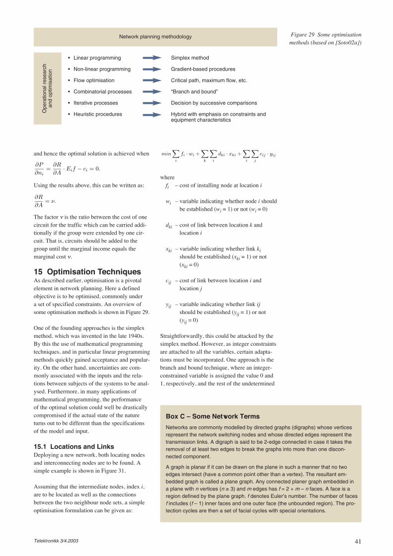
41Telektronikk 3/4.2003
wherefi – cost of installing node at location i
wi – variable indicating whether node i shouldbe established (wi = 1) or not (wi = 0)
dki – cost of link between location k andlocation i
xki – variable indicating whether link ki
should be established (xki = 1) or not(xki = 0)
cij – cost of link between location i andlocation j
yij – variable indicating whether link ijshould be established (yij = 1) or not(yij = 0)
Straightforwardly, this could be attacked by thesimplex method. However, as integer constraintsare attached to all the variables, certain adapta-tions must be incorporated. One approach is thebranch and bound technique, where an integer-constrained variable is assigned the value 0 and1, respectively, and the rest of the undetermined
Box C – Some Network Terms
Networks are commonly modelled by directed graphs (digraphs) whose verticesrepresent the network switching nodes and whose directed edges represent thetransmission links. A digraph is said to be 2-edge connected in case it takes theremoval of at least two edges to break the graphs into more than one discon-nected component.
A graph is planar if it can be drawn on the plane in such a manner that no twoedges intersect (have a common point other than a vertex). The resultant em-bedded graph is called a plane graph. Any connected planer graph embedded ina plane with n vertices (n ≥ 3) and m edges has f = 2 + m – n faces. A face is aregion defined by the plane graph. f denotes Euler’s number. The number of facesf includes (f – 1) inner faces and one outer face (the unbounded region). The pro-tection cycles are then a set of facial cycles with special orientations.
∂P
∂ni
=∂R
∂A· Eif − ci = 0.
∂R
∂A= ν.
and hence the optimal solution is achieved when
Network planning methodologyO
pera
tiona
l res
earc
h an
d op
timis
atio
n
• Linear programming Simplex method
• Non-linear programming Gradient-based procedures
• Flow optimisation Critical path, maximum flow, etc.
• Combinatorial processes “Branch and bound”
• Iterative processes Decision by successive comparisons
• Heuristic procedures Hybrid with emphasis on constraints andequipment characteristics
Figure 29 Some optimisationmethods (based on [Soto02a])
Using the results above, this can be written as:
The factor ν is the ratio between the cost of onecircuit for the traffic which can be carried addi-tionally if the group were extended by one cir-cuit. That is, circuits should be added to thegroup until the marginal income equals themarginal cost ν.
15 Optimisation TechniquesAs described earlier, optimisation is a pivotalelement in network planning. Here a definedobjective is to be optimised, commonly undera set of specified constraints. An overview ofsome optimisation methods is shown in Figure 29.
One of the founding approaches is the simplexmethod, which was invented in the late 1940s.By this the use of mathematical programmingtechniques, and in particular linear programmingmethods quickly gained acceptance and popular-ity. On the other hand, uncertainties are com-monly associated with the inputs and the rela-tions between subjects of the systems to be anal-ysed. Furthermore, in many applications ofmathematical programming, the performanceof the optimal solution could well be drasticallycompromised if the actual state of the natureturns out to be different than the specificationsof the model and input.
15.1 Locations and LinksDeploying a new network, both locating nodesand interconnecting nodes are to be found. Asimple example is shown in Figure 31.
Assuming that the intermediate nodes, index i,are to be located as well as the connectionsbetween the two neighbour node sets, a simpleoptimisation formulation can be given as:
min∑
i
fi · wi +
∑
k
∑
i
dki · xki +
∑
i
∑
j
cij · yij
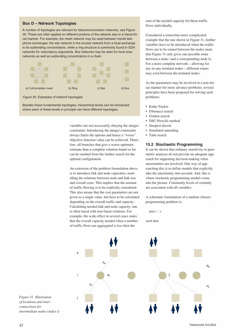
42 Telektronikk 3/4.2003
variables are not necessarily obeying the integerconstraints. Introducing the integer constraintsalways limits the options and hence a “worse”objective function value can be achieved. There-fore, all branches that give a worse optimumestimate than a complete solution found so farcan be omitted from the further search for theoptimal configuration.
An extension of the problem formulation aboveis to introduce link and node capacities; mod-elling the relations between node and link sizeand overall costs. This implies that the amountof traffic flowing is to be explicitly considered.This also means that the cost parameters are notgiven as a single value, but have to be calculateddepending on the overall traffic and capacity.Calculating needed link and node capacity, oneis often faced with non-linear relations. Forexample, the scale effect in several cases statesthat the overall capacity needed when a numberof traffic flows are aggregated is less then the
sum of the needed capacity for these trafficflows individually.
Considered a somewhat more complicatedexample that the one shown in Figure 31, furthervariables have to be introduced when the trafficflows are to be routed between the nodes (notethat Figure 31 only gives one possible routebetween a node i and a corresponding node k).For a more complete network – allowing forany-to-any terminal nodes – different routesmay exist between the terminal nodes.
As the parameters may be involved in a non-lin-ear manner for more advance problems, severalprinciples have been proposed for solving suchproblems:
• Kuhn-Tucker• Fibonacci search• Golden search• DSC-Powells method• Steepest decent• Simulated annealing• Tabu search
15.2 Stochastic ProgrammingIt can be shown that ordinary sensitivity or para-metric analyses do not provide an adequate app-roach for supporting decision-making whenuncertainties are involved. One way of app-roaching this is to define models that explicitlytake the uncertainty into account. And, this iswhere stochastic programming models comeinto the picture. Commonly levels of certaintyare associated with all variables.
A schematic formulation of a random (linear)programming problem is:
min c . x
such that
Box D – Network Topologies
A number of topologies are relevant for telecommunication networks, see Figure30. These are often applied on different portions of the network also in a hierarchi-cal manner. For example, the mesh network may be used between transit tele-phone exchanges, the star network in the access network from a local exchangeto its subtending concentrators, while a ring structure is commonly found in SDHnetworks for redundancy arguments. Bus networks may be seen for local areanetworks as well as subtending concentrators in a chain.
Besides these fundamental topologies, hierarchical levels can be introducedwhere each of these levels in principle can have different topologies.
Figure 30 Examples of network topologies
a) Full/complete mesh b) Ring c) Star d) Bus
k
xki
yij
wi fi
cij
dki
i
jFigure 31 Illustration of locations and inter-connections for intermediate nodes (index i)
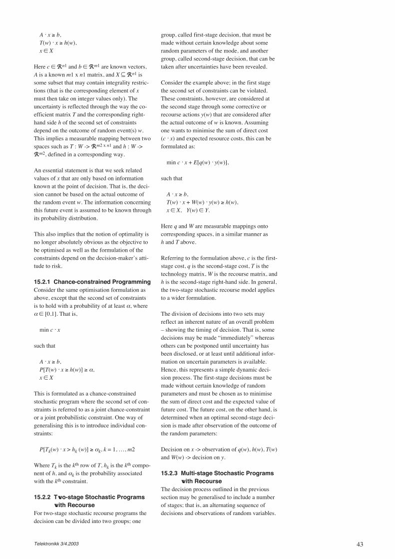
43Telektronikk 3/4.2003
A . x ≥ b,T(w) . x ≥ h(w),x ∈ X
Here c ∈ RRn1 and b ∈ RRm1 are known vectors,A is a known m1 x n1 matrix, and X ⊆ RRn1 issome subset that may contain integrality restric-tions (that is the corresponding element of xmust then take on integer values only). Theuncertainty is reflected through the way the co-efficient matrix T and the corresponding right-hand side h of the second set of constraintsdepend on the outcome of random event(s) w.This implies a measurable mapping between twospaces such as T : W -> RRm2 x n1 and h : W ->RRm2, defined in a corresponding way.
An essential statement is that we seek relatedvalues of x that are only based on informationknown at the point of decision. That is, the deci-sion cannot be based on the actual outcome ofthe random event w. The information concerningthis future event is assumed to be known throughits probability distribution.
This also implies that the notion of optimality isno longer absolutely obvious as the objective tobe optimised as well as the formulation of theconstraints depend on the decision-maker’s atti-tude to risk.
15.2.1 Chance-constrained ProgrammingConsider the same optimisation formulation asabove, except that the second set of constraintsis to hold with a probability of at least α, whereα ∈ [0,1]. That is,
min c . x
such that
A . x ≥ b,P[T(w) . x ≥ h(w)] ≥ α,x ∈ X
This is formulated as a chance-constrainedstochastic program where the second set of con-straints is referred to as a joint chance-constraintor a joint probabilistic constraint. One way ofgeneralising this is to introduce individual con-straints:
P[Tk(w) . x > hk (w)] ≥ αk, k = 1, …, m2
Where Tk is the kth row of T, hk is the kth compo-nent of h, and αk is the probability associatedwith the kth constraint.
15.2.2 Two-stage Stochastic Programswith Recourse
For two-stage stochastic recourse programs thedecision can be divided into two groups; one
group, called first-stage decision, that must bemade without certain knowledge about somerandom parameters of the mode, and anothergroup, called second-stage decision, that can betaken after uncertainties have been revealed.
Consider the example above; in the first stagethe second set of constraints can be violated.These constraints, however, are considered atthe second stage through some corrective orrecourse actions y(w) that are considered afterthe actual outcome of w is known. Assumingone wants to minimise the sum of direct cost(c . x) and expected resource costs, this can beformulated as:
min c . x + E[q(w) . y(w)],
such that
A . x ≥ b,T(w) . x + W(w) . y(w) ≥ h(w),x ∈ X, Y(w) ∈ Y.
Here q and W are measurable mappings ontocorresponding spaces, in a similar manner ash and T above.
Referring to the formulation above, c is the first-stage cost, q is the second-stage cost, T is thetechnology matrix, W is the recourse matrix, andh is the second-stage right-hand side. In general,the two-stage stochastic recourse model appliesto a wider formulation.
The division of decisions into two sets mayreflect an inherent nature of an overall problem– showing the timing of decision. That is, somedecisions may be made “immediately” whereasothers can be postponed until uncertainty hasbeen disclosed, or at least until additional infor-mation on uncertain parameters is available.Hence, this represents a simple dynamic deci-sion process. The first-stage decisions must bemade without certain knowledge of randomparameters and must be chosen as to minimisethe sum of direct cost and the expected value offuture cost. The future cost, on the other hand, isdetermined when an optimal second-stage deci-sion is made after observation of the outcome ofthe random parameters:
Decision on x -> observation of q(w), h(w), T(w)and W(w) -> decision on y.
15.2.3 Multi-stage Stochastic Programswith Recourse
The decision process outlined in the previoussection may be generalised to include a numberof stages; that is, an alternating sequence ofdecisions and observations of random variables.
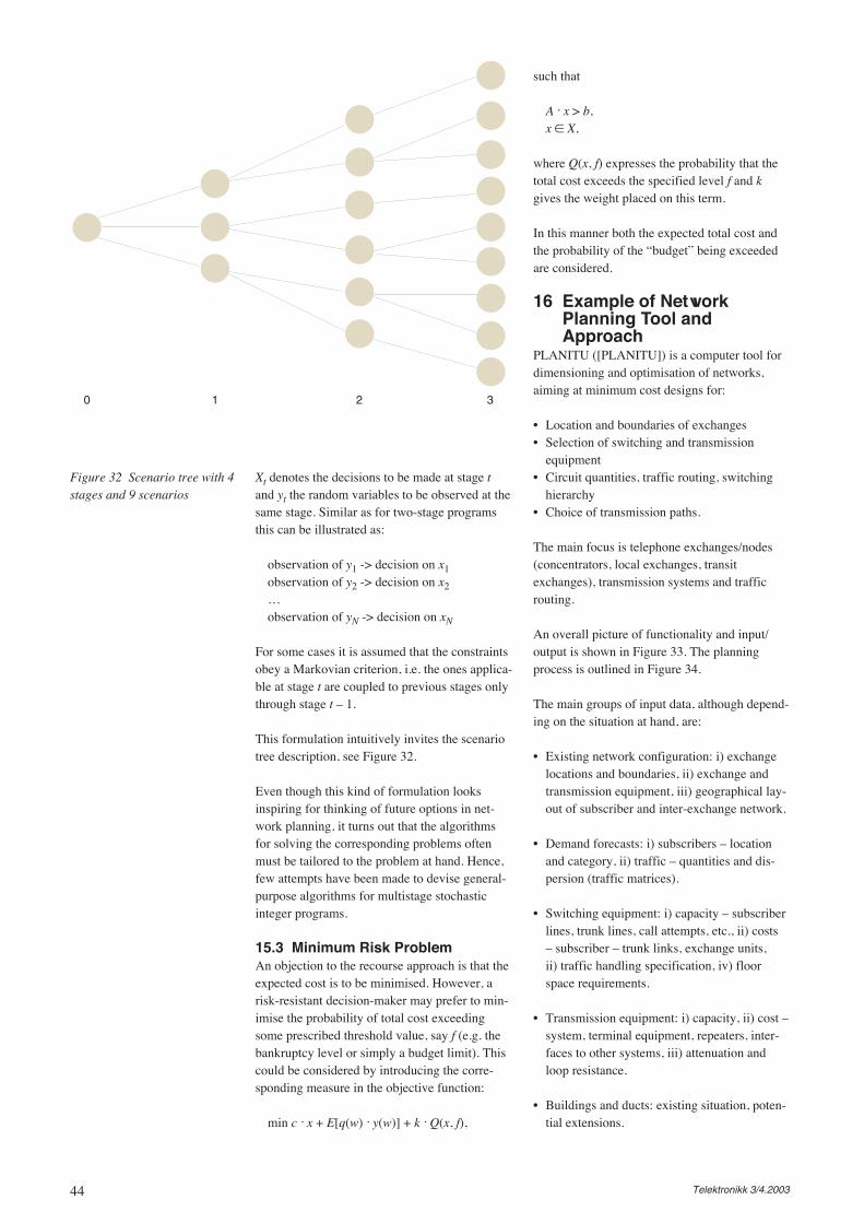
44 Telektronikk 3/4.2003
Xt denotes the decisions to be made at stage tand yt the random variables to be observed at thesame stage. Similar as for two-stage programsthis can be illustrated as:
observation of y1 -> decision on x1observation of y2 -> decision on x2…observation of yN -> decision on xN
For some cases it is assumed that the constraintsobey a Markovian criterion, i.e. the ones applica-ble at stage t are coupled to previous stages onlythrough stage t – 1.
This formulation intuitively invites the scenariotree description, see Figure 32.
Even though this kind of formulation looksinspiring for thinking of future options in net-work planning, it turns out that the algorithmsfor solving the corresponding problems oftenmust be tailored to the problem at hand. Hence,few attempts have been made to devise general-purpose algorithms for multistage stochasticinteger programs.
15.3 Minimum Risk ProblemAn objection to the recourse approach is that theexpected cost is to be minimised. However, arisk-resistant decision-maker may prefer to min-imise the probability of total cost exceedingsome prescribed threshold value, say f (e.g. thebankruptcy level or simply a budget limit). Thiscould be considered by introducing the corre-sponding measure in the objective function:
min c . x + E[q(w) . y(w)] + k . Q(x, f),
such that
A . x > b,x ∈ X,
where Q(x, f) expresses the probability that thetotal cost exceeds the specified level f and kgives the weight placed on this term.
In this manner both the expected total cost andthe probability of the “budget” being exceededare considered.
16 Example of NetworkPlanning Tool andApproach
PLANITU ([PLANITU]) is a computer tool fordimensioning and optimisation of networks,aiming at minimum cost designs for:
• Location and boundaries of exchanges• Selection of switching and transmission
equipment• Circuit quantities, traffic routing, switching
hierarchy• Choice of transmission paths.
The main focus is telephone exchanges/nodes(concentrators, local exchanges, transitexchanges), transmission systems and trafficrouting.
An overall picture of functionality and input/output is shown in Figure 33. The planningprocess is outlined in Figure 34.
The main groups of input data, although depend-ing on the situation at hand, are:
• Existing network configuration: i) exchangelocations and boundaries, ii) exchange andtransmission equipment, iii) geographical lay-out of subscriber and inter-exchange network.
• Demand forecasts: i) subscribers – locationand category, ii) traffic – quantities and dis-persion (traffic matrices).
• Switching equipment: i) capacity – subscriberlines, trunk lines, call attempts, etc., ii) costs– subscriber – trunk links, exchange units,ii) traffic handling specification, iv) floorspace requirements.
• Transmission equipment: i) capacity, ii) cost –system, terminal equipment, repeaters, inter-faces to other systems, iii) attenuation andloop resistance.
• Buildings and ducts: existing situation, poten-tial extensions.
0 1 2 3
Figure 32 Scenario tree with 4stages and 9 scenarios
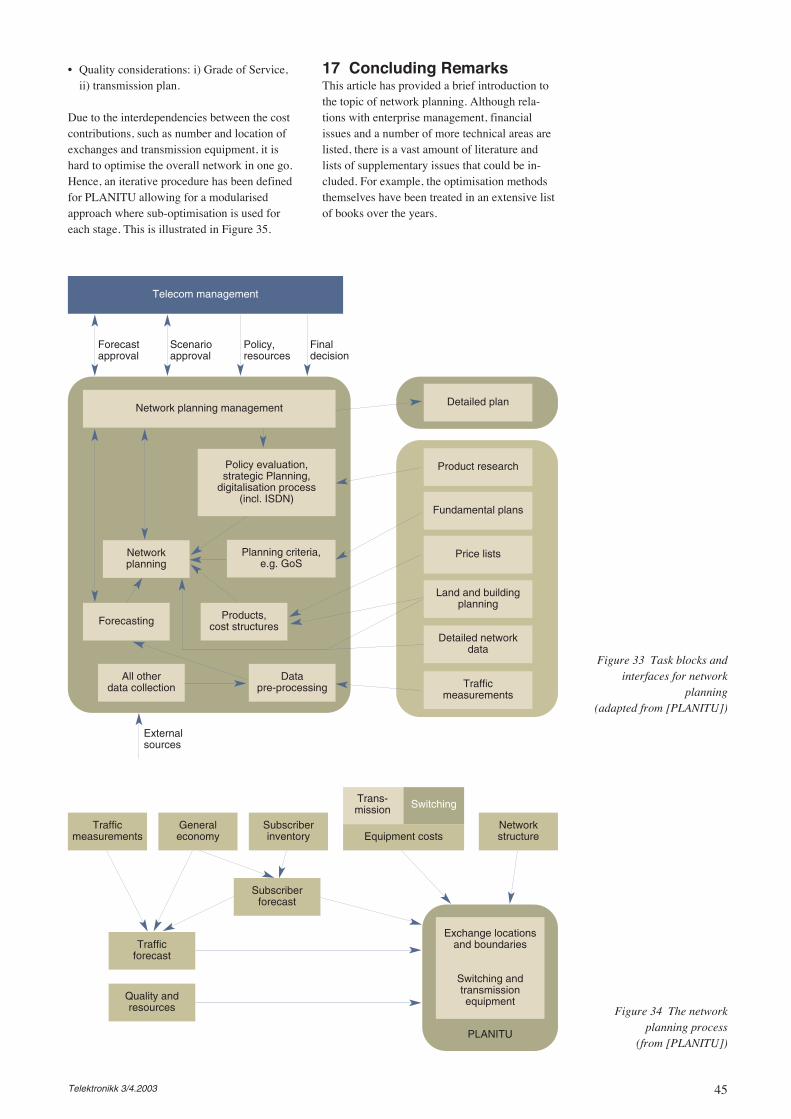
45Telektronikk 3/4.2003
• Quality considerations: i) Grade of Service,ii) transmission plan.
Due to the interdependencies between the costcontributions, such as number and location ofexchanges and transmission equipment, it ishard to optimise the overall network in one go.Hence, an iterative procedure has been definedfor PLANITU allowing for a modularisedapproach where sub-optimisation is used foreach stage. This is illustrated in Figure 35.
17 Concluding RemarksThis article has provided a brief introduction tothe topic of network planning. Although rela-tions with enterprise management, financialissues and a number of more technical areas arelisted, there is a vast amount of literature andlists of supplementary issues that could be in-cluded. For example, the optimisation methodsthemselves have been treated in an extensive listof books over the years.
Telecom management
Network planning management
Networkplanning
Forecasting Products,cost structures
All otherdata collection
Datapre-processing
Policy evaluation,strategic Planning,
digitalisation process(incl. ISDN)
Planning criteria,e.g. GoS
Product research
Fundamental plans
Price lists
Land and buildingplanning
Detailed networkdata
Trafficmeasurements
Detailed plan
Externalsources
Forecastapproval
Scenarioapproval
Policy,resources
Finaldecision
Figure 33 Task blocks andinterfaces for network
planning (adapted from [PLANITU])
Trans-mission Switching
Trafficmeasurements
Trafficforecast
Quality andresources
Generaleconomy
Subscriberinventory Equipment costs
Networkstructure
Subscriberforecast
Exchange locationsand boundaries
Switching andtransmissionequipment
PLANITU
Figure 34 The networkplanning process
(from [PLANITU])
46 Telektronikk 3/4.2003
A key message in this presentation is that net-work planning is multi-faceted and has relationswith (almost) all other types of activities goingon in a network operator. Hence, it is importantto balance the system portfolio insight withskills in planning techniques as well as the finan-cial means for comparing results. In additioncomes the different time horizons one has todeal with – from strategic planning to tuning ofparameters for traffic handling.
A key point for an operator is to provide the setof services asked for by the customers – and thisshould be done more cost-effectively and fasterthan the competitors. As shown in Figure 36 thecustomers’ demands can often be arranged alonga scale with the corresponding service levels.Whether this is done by a single network or notis not shown in the illustration.
The increasing awareness of network planningis particularly crucial when efficiency improve-ments are to be implemented in an organisation.In fact, the systematic views that network plan-ning techniques provide also support thesmoother interactions between units within theorganisation as well as between the operatorsand other actors in the market.
References[DSL-058] DSL forum. Multi-Service Architec-ture & Framework Requirements. September2003. Technical Report TR-058. (www.dslforum.org)
[Macf02] MacFadyen, N W. Traffic characteri-sation and modelling. BT Technology Journal,20 (3), 14–30, 2002.
[PLANITU] ITU-D PLANITU Network Plan-ning Software. Februar 25, 2004 [online] – URL:www.itu.int/ITU-D/planitu/index.html 2003
[RFC372] Awduche, D et al. Overview andPrinciples of Internet Traffic Engineering. IETFRFC 3272, May 203.
[Sing02] Singleton, P. Performance modelling –what, why, when and how. BT Technology Jour-nal, 20 (3), 133–143, 2002.
[Soto02] Soto, O. Integrated Planning method-ology. Scenario analysis and data gathering.ITU-D workshop on network planning strategiesfor evolving network architectures, Nairobi,Kenya, 7–11 October 2002.
[Soto02a] Soto, O. Requirements for decisionmaking in network evolution, Strategic planningand new Technologies, Solution mapping forgeo-scenarios. ITU-D workshop on networkplanning strategies for evolving network archi-tectures, Nairobi, Kenya, 7–11 October 2002.
Exchangelocations
BoundariesCircuits
Input: Output:
LocationsDistances
Exchangeboundaries
LocationsCost/erlang
BoundariesSubs/exchange
Inter-exchangetraffic
BoundariesSubs/exchange
Trafficdistribution
Inter-exchangecircuits
TrafficCost/circuit
CircuitsRouting
CircuitsDistances
Cost/linkCost/circuit
Transmissionsystems
Currentnetwork
Improvednetwork
Networkchanges
Figure 35 Activities forexchange network planning,based on [PLANITU]
Price (service level) Price (service level) Price (service level)
Number of customers Number of customers Number of customers
Figure 36 Illustrating theawareness of diverse demandsand offering adequate servicelevels and price levels mayimprove the operator’smargins
47
1 IntroductionThe rapid technological development in thetelecommunications field during the last twodecades made it necessary for the operators torepeatedly reevaluate the structure, design andapplication of their networks. In order to estab-lish cost-effective network design and utilizationmany telecommunication operators developedand used optimization-based network planningtools. This happened also in Telenor. The ratio-nale was that the frequent technological shiftsdid not give the planners sufficient time toacquire an intuitive feeling of what constitutedgood network designs. So the requirement forcomprehensive, cost-effective and robustdesigns excluded simple back of the envelopeor spread sheet calculations. The idea was thatmathematical models could be used to optimizenetwork structures and thus contribute to reducecosts, ensure network reliability and improveoperational efficiency.
The approach was said to be pragmatic but thor-ough; heuristic but nevertheless intelligent. Theaim was not to give a black box answer, but adeeper understanding of the issues and of theconsequences of proposed solutions. The opti-mization tools were not meant to give a finalanswer, but to constitute instruments to be inte-grated into the decision process of the planners.
Common to all the tools were that they werebased on mathematical programming. The dif-ferent network components were modeled asdecision variables with associated costs. Techno-logical constraints were modeled by equationsand inequalities that the decision variables hadto satisfy. Commercially available optimizationsoftware together with tailor-made programmodules were used to find cost-effective solu-tions. The fact that the tools were to be used byothers than the ones who developed them im-plied that they had to be incorporated in highquality user interfaces and linked up to relevantdata sources in an appropriate way. In generalthe effort spent on the development of user inter-faces exceeded the effort spent on implementa-tion of optimization algorithms by a factor ofthree to four.
In 1986 Telenor R&D together with the consul-tant company Veritas established a group ofthree people who started building optimizationmodels for key network design problems.Telenor R&D was mainly responsible for the
modelling whilst Veritas was given the task ofimplementing the models. Later on the consul-tants at Veritas moved to the consultant com-pany Computas, and the cooperation with Com-putas has continued to this day.
From the outset a good cooperation was estab-lished with network operators in the field whoallocated time and energy to specification andtesting.
The initiative was triggered by a situation wherea local cable TV network planner compared twoalternative network layouts which both seemedreasonable, but discovered afterwards that thecost of one of the layouts was twice the cost ofthe other. The group worked together on and offover a period of about 15 years and designed andimplemented a series of network planning toolsbased on integer programming. Some of thetools will be described in the sequel, namelyKABINETT, ABONETT, FABONETT,PETRA, MOBANETT, and MOBINETT.
2 KABINETT – A Cable TV Net-work Planning Tool
2.1 GeneralAt the time when the cable TV network planningtool KABINETT was developed the networksshould have a tree structure. Manual planningwas time-consuming, and the planners hadcapacity for analyzing a few alternatives only.One important feature of the planning problemwas to secure that the subscribers received suffi-cient voltage with a minimum number of ampli-fiers. Also, the cost of civil work constituted alarge portion of the total cost. Of course, theplanning problem became much simpler laterwhen the decision was made to go for star net-works in lieu of tree networks.
2.2 The Cable TV Network DesignProblem
Here will be given a short description of thecable TV network design problem KABINETTattempted to solve.
We were given a signal source and a set of sub-scribers. The signal source was to be connectedto the subscribers by copper cables via ampli-fiers, splitters and taps.
The amplifiers, splitters and taps had to beplaced in cabinets. There were two types of cabi-
Optimization-Based Network Planning Toolsin Telenor During the Last 15 Years – A SurveyR A L P H L O R E N T Z E N
Ralph Lorentzen (67) is dailyleader of the companyLorentzen LP Service whichdoes consulting work withinmathematical programming. Heretired July 1, 2003 from his jobas senior scientist in TelenorR&D. Ralph Lorentzen gradu-ated in mathematics at the Uni-versity of Oslo, where heworked for some time as assis-tant professor giving lectures instatistics and operationsresearch. He worked as distribu-tion planner in Norske Esso, asprincipal scientist at ShapeTechnical Centre, as systemsengineer in IBM, and as chiefconsultant in Control Data Nor-way, before joining Telenor R&Din 1985.
Telektronikk 3/4.2003
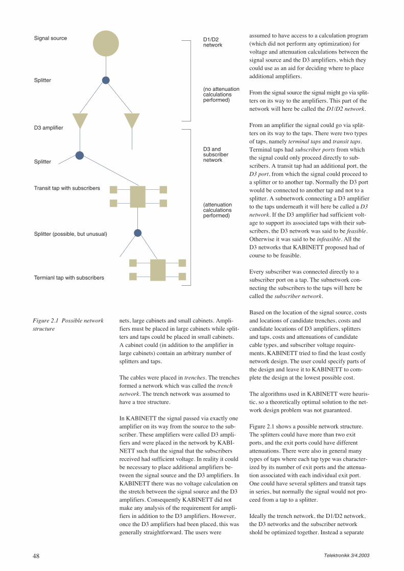
48 Telektronikk 3/4.2003
nets, large cabinets and small cabinets. Ampli-fiers must be placed in large cabinets while split-ters and taps could be placed in small cabinets.A cabinet could (in addition to the amplifier inlarge cabinets) contain an arbitrary number ofsplitters and taps.
The cables were placed in trenches. The trenchesformed a network which was called the trenchnetwork. The trench network was assumed tohave a tree structure.
In KABINETT the signal passed via exactly oneamplifier on its way from the source to the sub-scriber. These amplifiers were called D3 ampli-fiers and were placed in the network by KABI-NETT such that the signal that the subscribersreceived had sufficient voltage. In reality it couldbe necessary to place additional amplifiers be-tween the signal source and the D3 amplifiers. InKABINETT there was no voltage calculation onthe stretch between the signal source and the D3amplifiers. Consequently KABINETT did notmake any analysis of the requirement for ampli-fiers in addition to the D3 amplifiers. However,once the D3 amplifiers had been placed, this wasgenerally straightforward. The users were
assumed to have access to a calculation program(which did not perform any optimization) forvoltage and attenuation calculations between thesignal source and the D3 amplifiers, which theycould use as an aid for deciding where to placeadditional amplifiers.
From the signal source the signal might go via split-ters on its way to the amplifiers. This part of thenetwork will here be called the D1/D2 network.
From an amplifier the signal could go via split-ters on its way to the taps. There were two typesof taps, namely terminal taps and transit taps.Terminal taps had subscriber ports from whichthe signal could only proceed directly to sub-scribers. A transit tap had an additional port, theD3 port, from which the signal could proceed toa splitter or to another tap. Normally the D3 portwould be connected to another tap and not to asplitter. A subnetwork connecting a D3 amplifierto the taps underneath it will here be called a D3network. If the D3 amplifier had sufficient volt-age to support its associated taps with their sub-scribers, the D3 network was said to be feasible.Otherwise it was said to be infeasible. All theD3 networks that KABINETT proposed had ofcourse to be feasible.
Every subscriber was connected directly to asubscriber port on a tap. The subnetwork con-necting the subscribers to the taps will here becalled the subscriber network.
Based on the location of the signal source, costsand locations of candidate trenches, costs andcandidate locations of D3 amplifiers, splittersand taps, costs and attenuations of candidatecable types, and subscriber voltage require-ments, KABINETT tried to find the least costlynetwork design. The user could specify parts ofthe design and leave it to KABINETT to com-plete the design at the lowest possible cost.
The algorithms used in KABINETT were heuris-tic, so a theoretically optimal solution to the net-work design problem was not guaranteed.
Figure 2.1 shows a possible network structure.The splitters could have more than two exitports, and the exit ports could have differentattenuations. There were also in general manytypes of taps where each tap type was character-ized by its number of exit ports and the attenua-tion associated with each individual exit port.One could have several splitters and transit tapsin series, but normally the signal would not pro-ceed from a tap to a splitter.
Ideally the trench network, the D1/D2 network,the D3 networks and the subscriber networkshold be optimized together. Instead a separate
Figure 2.1 Possible networkstructure
Signal source
Splitter
D3 amplifier
Transit tap with subscribers
Splitter
Splitter (possible, but unusual)
Termianl tap with subscribers
D1/D2network
(no attenuationcalculationsperformed)
D3 andsubscribernetwork
(attenuationcalculationsperformed)
49Telektronikk 3/4.2003
cost minimization of the trench network wasdone first. Then an optimization of the sub-scriber network was done followed by the opti-mization of the D3 networks, and finally theD1/D2 network was determined. The separateoptimization of the trench network was partlyjustified by the fact that usually well above 70 %of the total network cost was the cost of trenches.
2.3 InputThe input to KABINETT specified
• the location of the subscribers to be connectedto the network
• the location of the signal source node• the location of the nodes where D3 amplifiers,
splitters and taps could be placed• trench route alternatives• cable types• splitter types• tap types• the D3 amplifier type• cabinet types
The trench routes consisted of trench sections,each of which was characterized by geographicallocation, length, and cost per metre.
The cable types were characterized by attenua-tion and cost per metre.
The splitter types were characterized by thenumber of ports and the attenuation at each indi-vidual port.
The tap types were characterized by the numberof ports and the attenuation at each individualport and whether they were transit taps or termi-nal taps.
KABINETT operated with one type of D3amplifier which was characterized by cost andthe voltage at the exit port.
There were two cabinet types, namely large andsmall. Each type was characterized by cost.
2.4 OutputThe output from KABINETT described the pro-posed solution to the cable TV network designproblem. It showed• the trenches to be dug• what types of cables should be used where• where D3 amplifiers should be placed• what type of splitters and taps should be
placed where• which subscribers should be connected to
which ports on which taps• a table showing labour costs and bill of mate-
rials
The output could be fed into an interactive cal-culation program (not described here) for place-ment of amplifiers in the D1/D2 network. Thisprogram also gave a schematic description of thesolution.
2.5 Determining the Trench NetworkThe trench network cost minimization problemis an example of the classical Steiner problemin undirected graphs. A network of candidatetrenches was given, and the problem was to findthe cheapest possible subnetwork (which mustnecessarily be a tree) which connected a subsetof nodes. The nodes to be connected includedthe signal source node and the subscriber nodes.In addition the planner could include amongstthe special nodes some of the equipment nodes,i.e. candidate nodes for placement of D3 ampli-fiers, splitters and/or taps.
There could be subscribers who were connectedto the rest of the candidate trench network bytwo or more candidate trenches. However, onemight want to avoid using these candidatetrenches for transit cables to other subscribers.This was achieved by multiplying the cost ofthese trenches by a large number before the opti-mization.
In KABINETT an approximate solution to theSteiner problem was found using Rayward-Smith’s algorithm [1].
2.6 Determining the SubscriberNetwork
The model used for the subscriber network wasa classical capacitated plant location model.
The subscribers were to be connected to taps bycables. In this module all taps were consideredto be terminal taps. One cable type only wasconsidered for each subscriber. In practice theplanner would assume a default cable type forall subscribers in an initial run. As a result of in-specting the initial solution he could change thecable type for some of the subscribers and runthe optimization again.
Each candidate tap was given a cost which wasthe sum of the tap cost, the cost of a small cabi-net, and the cost of the copper cable needed toconnect the tap to the closest equipment nodein the direction of the signal source node.
The cost of connecting a given subscriber to atap in a given equipment node was set to the sumof the material and labour cost associated withconnecting them with the appropriate cable.
Attenuation was not considered in the subscribernetwork optimization. Voltage and attenuation
50 Telektronikk 3/4.2003
considerations were postponed to the D3 net-work optimization.
The subscriber network optimization model isdescribed in mathematical terms below.
The following notation is used:
Subscripts
n denotes equipment nodes,s denotes subscribers,t denotes terminal tap types.
Costs
cns denotes the cost of connecting subscriber s toequipment node n;cnt denotes the cost of placing a terminal tap oftype t in equipment node n. This cost is the sumof the tap cost and the cost of a cable from thetap to the nearest equipment node on the route tothe signal source node.
Capacities
pt denotes the number of subscriber ports on atap of type t.
Variables
xns = 1 if subscriber s should be connected to atap in equipment node n, and = 0 otherwise.
ynt = 1 if a tap of type t should be placed inequipment node n, and = 0 otherwise.
Using this notation the optimization problem canbe formulated as follows:
minimize Σnscnsxns + Σntcntynt (2.1)
subject to
Σnxns = 1 (2.2)
Σsxns ″ Σtptynt (2.3)
xns ″ Σtynt (2.4)
where xns and ynt are 0 – 1 variables.
This optimization problem was solved using aconventional branch and bound code.
The planner could preset part of the solution byfixing some of the xns or ynt variables to 1.
When the subscriber network was determined,the voltage requirement at the taps were calcu-lated and recorded.
2.7 Determining the D3 Network
2.7.1 GeneralThe method for determining the D3 networksconsisted of three algorithms, namely the con-struction algorithm, the partitioning algorithmand the move/exchange algorithm.
Typically, KABINETT started with attemptingto cover all the taps with one D3 amplifier. Ifthis failed, two D3 amplifiers were tried, etc. Ifthe minimum number of D3 amplifiers whichKABINETT found was needed was K, and theparameter ‘extra’ was set to a positive integer,then KABINETT tried to find the least expen-sive solution with K, K + 1, …, or K + extraamplifiers.
The construction algorithm took as input a sub-set of the taps with their voltage requirementsand placed a D3 amplifier in a node such thateither a feasible D3 network was formed or an(infeasible) D3 network was formed where thevoltage requirement in the D3 amplifier nodewas as low as possible.
The partitioning algorithm was a one pass algo-rithm for partitioning the taps into a specifiednumber of subsets and constructing a (feasibleor infeasible) D3 network for each of the subsets.
The move/exchange algorithm was an iterativealgorithm which tried to improve on the solutionfound by the partitioning algorithm. The move/exchange algorithm tried first of all to make aninfeasible solution feasible, and tried thereafterto find a solution with reduced cost.
Before we treat these algorithms we willdescribe the splap concept.
2.7.2 SplapsIn the D3 network KABINETT could placemore than one splitter and/or tap in an equip-ment node. The result was a collection of split-ters and taps which could be characterized by itstotal cost, a set of D3 ports with their individualattenuations, and a set of subscriber ports withtheir individual attenuations. Such a collectionof splitters and taps in a node was in KABI-NETT denoted a splap (see Figure 2.2).
Before the D3 network optimization was startedKABINETT compiled a list of candidate splapsbased on the splitter and tap types in the input.As mentioned earlier the D3 port of a transit tapwould normally be connected to another tap andnot to a splitter, and the splap list was based oncollections of splitters and taps where this wasthe case. The planner decided the size of this listby specifying the maximal number of subscriberand D3 ports of the splaps.
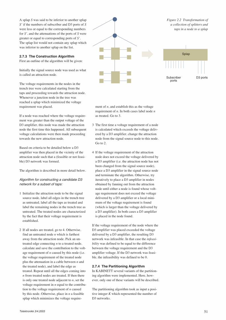
51Telektronikk 3/4.2003
A splap S was said to be inferior to another splapS’ if the numbers of subscriber and D3 ports of Swere less or equal to the corresponding numbersfor S’, and the attenuations of the ports of S weregreater or equal to corresponding ports of S’.The splap list would not contain any splap whichwas inferior to another splap on the list.
2.7.3 The Construction AlgorithmFirst an outline of the algorithm will be given:
Initially the signal source node was used as whatis called an attraction node.
The voltage requirements in the nodes in thetrench tree were calculated starting from thetaps and proceeding towards the attraction node.Whenever a junction node in the tree wasreached a splap which minimized the voltagerequirement was placed.
If a node was reached where the voltage require-ment was greater than the output voltage of theD3 amplifier, this node was made the attractionnode the first time this happened. All subsequentvoltage calculations were then made proceedingtowards the new attraction node.
Based on criteria to be detailed below a D3amplifier was then placed in the vicinity of theattraction node such that a (feasible or not feasi-ble) D3 network was formed.
The algorithm is described in more detail below.
Algorithm for constructing a candidate D3network for a subset of taps:
1 Initialize the attraction node to be the signalsource node, label all edges in the trench treeas untreated, label all the taps as treated andlabel the remaining nodes in the trench tree asuntreated. The treated nodes are characterizedby the fact that their voltage requirement isestablished.
2 If all nodes are treated, go to 4. Otherwise,find an untreated node n which is farthestaway from the attraction node. Pick an un-treated edge connecting n to a treated node,calculate and save the contribution to the volt-age requirement of n caused by this node (i.e.the voltage requirement of the treated nodeplus the attenuation in a cable between n andthe treated node), and label the edge astreated. Repeat until all the edges coming inton from treated nodes are treated. If then thereis only one treated node adjacent to n, set thevoltage requirement in n equal to the contribu-tion to the voltage requirement of n causedby this node. Otherwise, place in n a feasiblesplap which minimizes the voltage require-
ment of n, and establish this as the voltagerequirement of n. In both cases label node nas treated. Go to 3.
3 The first time a voltage requirement of a nodeis calculated which exceeds the voltage deliv-ered by a D3 amplifier, change the attractionnode from the signal source node to this node.Go to 2.
4 If the voltage requirement of the attractionnode does not exceed the voltage delivered bya D3 amplifier (i.e. the attraction node has notbeen changed from the signal source node),place a D3 amplifier in the signal source nodeand terminate the algorithm. Otherwise, tryiteratively to place a D3 amplifier in nodesobtained by fanning out from the attractionnode until either a node is found whose volt-age requirement does not exceed the voltagedelivered by a D3 amplifier or a local mini-mum of the voltage requirement is found(which is larger than the voltage delivered bya D3 amplifier). In both cases a D3 amplifieris placed in the node found.
If the voltage requirement of the node where theD3 amplifier was placed exceeded the voltagedelivered by a D3 amplifier, the resulting D3network was infeasible. In that case the infeasi-bility was defined to be equal to the differencebetween the voltage requirement and the D3amplifier voltage. If the D3 network was feasi-ble, the infeasibility was defined to be 0.
2.7.4 The Partitioning AlgorithmIn KABINETT several variants of the partition-ing algorithm were implemented. Here, how-ever, only one of these variants will be described.
The partitioning algorithm took as input a posi-tive integer K which represented the number ofD3 networks.
Subscriberports
D3 ports
Splap
Figure 2.2 Transformation ofa collection of splitters and
taps in a node to a splap
52 Telektronikk 3/4.2003
A description of the partitioning algorithm fol-lows.
Partitioning algorithm for creating K(feasible or infeasible) D3 networks:
1 Start with all the K networks empty. Select theK taps which are farthest apart, i.e. the K tapst1, …, tK which maximize mini<j d(ti, tj).Include one of these taps in each of the Knetworks. Go to 2.
2 For each network find its close node, i.e. theclosest node which has not been included inany of the networks. If none of the networkshave a close node, terminate (every node be-longs to a network). Otherwise, order theclose nodes in a list according to how closethey are to their associated network. Labelall the close nodes as untreated. Go to 3.
3 If there are no untreated nodes, go to 5. Other-wise, go to 4.
4 Pick the first untreated close node on the list.If this close node does not contain a tap, in-clude the node in its associated network, andgo to 2. If the close node contains a tap andthe node can be included in its associated net-work without making the network infeasible(this is checked by the construction algorithm),make this inclusion and go to 2. Otherwise,label the close node as treated and go to 3.
5 Include the first close node on the list andgo to 2.
2.7.5 The Move/Exchange AlgorithmWhen a solution was found by the partitioningalgorithm, it was natural to try to improve on it.Whether the solution is feasible or not, attemptswere made to change it into a feasible solutionwith the same number of D3 amplifiers, andwith the lowest cost possible. This was the func-tion of the move/exchange algorithm.
In the description of the move/exchange algo-rithm the following concepts will be used:
Let N1 and N2 denote D3 networks and let tdenote a tap.
If N2 is infeasible with t in N1, let r1(t, N1, N2)denote the reduction in the sum of infeasibilitiesobtained by moving t to N2.
If N1 is feasible with t in N1, and if N2 is feasibleafter t is moved to N2, let rC(t, N1, N2) denote thereduction in cost obtained by moving t.
If N1 is infeasible with t in N1 or if N2 is infeasi-ble after t is moved to N2, let rV(t, N1, N2) denotethe reduction in the sum of voltage requirementsobtained by moving t to N2.
Now we can describe the move/exchange algo-rithm.
Move/exchange algorithm between acollection of D3 networks:
1 If all networks are feasible, go to 2. Other-wise, calculate r = max r1(t, N1, N2) where themaximization is done over all N1, N2 and t inN1. If r > 0, make a move which gives theinfeasibility reduction r. Repeat until either allnetworks are feasible or r ″ 0. If all networksare feasible, go to 2. If r ″ 0 and 3 has beenexecuted – stop, otherwise, go to 3.
2 Calculate r = max rC(t, N1, N2) (as usualmaximization over the empty set is definedto be –∞), where the maximization is doneover all t, N1 and N2 for which rC(t, N1, N2) isdefined.If r > 0, make a move which gives the costreduction r. Repeat until r < 0. If 4 has beenexecuted, terminate. Otherwise, go to 4.
3 Calculate max rV(t, N1, N2) and max rV(t, N2,N1), where the maximizations are made overall t, N1 and N2 for which the expressions aredefined. Let t1 and t2 be taps which maximizethe two expressions respectively. If moving t1from N1 to N2 and t2 from N2 to N1 results in areduction in the sum of infeasibilities, do thesemoves. (This is an ‘exchange’.) Repeat untilall networks are feasible or no reduction ininfeasibility results. If all networks are feasi-ble, go to 4. Otherwise, go to 1.
4 Calculate max rC(t, N1, N2) and max rC(t, N2,N1), where the maximizations are made overall t, N1 and N2 for which the expressions aredefined. Let t1 and t2 be taps which maximizethe two expressions respectively. If moving t1from N1 to N2 and t2 from N2 to N1 results ina reduction in cost, do these moves. Repeat aslong as cost reduction results. Then go to 2.
2.8 Determining the D1/D2 networkOnce the D3 networks were determined the de-termination of the D1/D2 network was straight-forward. KABINETT just cabled up the trenchtree which connects the D3 amplifiers with thesignal source node, and placed appropriate split-ters wherever necessary.
As mentioned earlier no voltage and attenuationcalculation was done in the D1/D2 network, soKABINETT did not place amplifiers in this net-work.
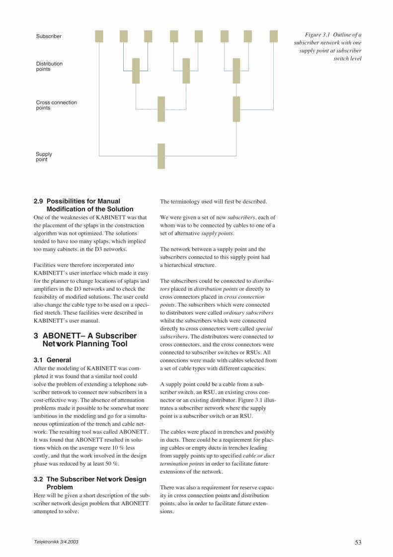
53Telektronikk 3/4.2003
2.9 Possibilities for ManualModification of the Solution
One of the weaknesses of KABINETT was thatthe placement of the splaps in the constructionalgorithm was not optimized. The solutionstended to have too many splaps, which impliedtoo many cabinets, in the D3 networks.
Facilities were therefore incorporated intoKABINETT’s user interface which made it easyfor the planner to change locations of splaps andamplifiers in the D3 networks and to check thefeasibility of modified solutions. The user couldalso change the cable type to be used on a speci-fied stretch. These facilities were described inKABINETT’s user manual.
3 ABONETT– A SubscriberNetwork Planning Tool
3.1 GeneralAfter the modeling of KABINETT was com-pleted it was found that a similar tool couldsolve the problem of extending a telephone sub-scriber network to connect new subscribers in acost-effective way. The absence of attenuationproblems made it possible to be somewhat moreambitious in the modeling and go for a simulta-neous optimization of the trench and cable net-work. The resulting tool was called ABONETT.It was found that ABONETT resulted in solu-tions which on the average were 10 % lesscostly, and that the work involved in the designphase was reduced by at least 50 %.
3.2 The Subscriber Network DesignProblem
Here will be given a short description of the sub-scriber network design problem that ABONETTattempted to solve.
The terminology used will first be described.
We were given a set of new subscribers, each ofwhom was to be connected by cables to one of aset of alternative supply points.
The network between a supply point and thesubscribers connected to this supply point hada hierarchical structure.
The subscribers could be connected to distribu-tors placed in distribution points or directly tocross connectors placed in cross connectionpoints. The subscribers which were connectedto distributors were called ordinary subscriberswhilst the subscribers which were connecteddirectly to cross connectors were called specialsubscribers. The distributors were connected tocross connectors, and the cross connectors wereconnected to subscriber switches or RSUs. Allconnections were made with cables selected froma set of cable types with different capacities.
A supply point could be a cable from a sub-scriber switch, an RSU, an existing cross con-nector or an existing distributor. Figure 3.1 illus-trates a subscriber network where the supplypoint is a subscriber switch or an RSU.
The cables were placed in trenches and possiblyin ducts. There could be a requirement for plac-ing cables or empty ducts in trenches leadingfrom supply points up to specified cable or ducttermination points in order to facilitate futureextensions of the network.
There was also a requirement for reserve capac-ity in cross connection points and distributionpoints, also in order to facilitate future exten-sions.
Figure 3.1 Outline of asubscriber network with one
supply point at subscriberswitch level
Subscriber
Distributionpoints
Cross connectionpoints
Supplypoint
54 Telektronikk 3/4.2003
The ABONETT user specified the subscribers,candidate supply points, candidate trenches, can-didate cross connection points and distributionpoints, and requirements for cables/ducts tospecified cable/duct termination points.
ABONETT tried to find a network design whichsatisfied all the given requirements and whichwas as inexpensive as possible.
The ABONETT user had full control over thesolution in the sense that he could specify asmany characteristics of the design as he wanted.In the extreme he could specify the solutioncompletely and use ABONETT just to check thevalidity of the solution and calculate its cost.
3.3 InputThe input to ABONETT described the sub-scribers to be connected to the network, the sup-ply point(s), cross connection and distributionpoint alternatives, reserve capacity requirements,cable or duct requirements (if any), and trenchroute alternatives.
The trench routes consisted of trench sections,each of which was characterized by geographicallocation, length and the required trench type. Incertain cases it was desired to reserve trenchusage. If a subscriber could connect to the net-work via more than one trench alternativethrough his property, it was important to preventABONETT from considering the possibility ofusing these trench alternatives as “transittrenches” for reaching other subscribers. Techni-cally this was treated in ABONETT by adding ahigh artificial cost to such trenches.
The trench types were described by cost permetre.
The subscribers were characterized by their geo-graphical location, the capacity they required,whether they should be connected to a distribu-tion point or directly to a cross connection point,and whether the adjacent trench sections shouldbe reserved.
The supply points were characterized by theirgeographical location, whether they wereswitches/RSUs, cross connectors or distributors,capacity, reserve capacity requirement, and max-imal distance to cross connection points, cabletermination points, distribution points or sub-scribers they could offer connection to.
The cross connection points were characterizedby their geographical location, the types of crossconnectors which could be placed there, the re-quired reserve capacity in percent, and maximaldistance to distribution points or special sub-scribers they could offer connection to.
The distribution points were likewise character-ized by their geographical location, the types ofdistributors which could be placed there, therequired spare capacity in percent, and maximaldistance to subscribers they could offer connec-tion to.
The cross connector types, distributor types,cable types, and ducts were characterized bycapacity and cost.
3.4 OutputThe output from ABONETT described the pro-posed solution to the subscriber network designproblem.
It listed the supply points, cross connectionpoints and distribution points with the equipmentselected by ABONETT, which trenches shouldbe dug, and which cables and ducts should beused. A simplified bill of materials was alsogiven.
3.5 The Trench and the CableNetworks
Two networks were introduced, namely an un-directed trench network and a directed cable net-work.
The edges in the trench network were the trenchsections, and the nodes were the end points ofthe trench sections.
The nodes in the cable network representedexisting supply points, existing and candidatecross connection and distribution points, sub-scribers, and cable/duct termination points. Inaddition an extra node was introduced, namelythe root node.
The arcs in the cable network connected the rootnode to the supply points, the supply points tothe cross connection points and cable/duct termi-nation points, the cross connection points to thedistribution points and special subscribers, andthe distribution points to the ordinary subscribers.
The cable network thus constituted a rooteddirected acyclic graph.
3.6 The Trench, Cable andCombined Optimizations
In order to keep the computation time withinreasonable limits three optimizations were made;namely the cable optimization, the trench opti-mization, and the combined optimization.
In the cable optimization ABONETT tried tofind the cheapest cabling which satisfied all therequirements under the assumption that all thetrenches are available free of charge.
55Telektronikk 3/4.2003
In the trench optimization ABONETT first triedto find the cheapest trench network which con-nected together the subscribers, the supplypoints, the cross connection points, the distribu-tion points, and the duct/cable terminationpoints. Then ABONETT tried to find the cheap-est cabling in this trench network which satisfiedall the requirements.
In the combination optimization ABONETTconsidered both trench costs and cable costs.However, the only trenches which were takeninto consideration were those selected either inthe trench optimization or in the cable optimiza-tion (or both). Trenches which were selectedboth in the trench and cable optimization, and inthe trench optimization were selected to containeither two or more cables or at least one cableterminating at a subscriber, are made available atno cost. All other trenches which were selectedeither in the cable or the trench optimizationwere made available at their real digging cost ifthey belonged to a circle in the resulting trenchnetwork, and at no cost if they did not belong toa circle.
The solution resulting from the combinationoptimization was ABONETT’s suggested solu-tion to the network design problem.
3.7 Finding the Cheapest PossibleTrench Network
In the trench optimization the cheapest trenchnetwork connecting the subscribers, cross con-nection points, distribution points and the duct/cable termination points was sought. It is obvi-ous that the cheapest network is a tree.
This was an example of the classical Steinerproblem in undirected graphs. In ABONETTan approximate solution to the Steiner problemis found using Rayward-Smith’s algorithm [1].
3.8 The Integer Programming Modelfor Finding the Cheapest Cablingin a Given Trench Network
The problem of finding the cheapest cabling in agiven trench network was in ABONETT formu-lated as an integer linear programming problem.
The following notation was used:
xijt = 1 if there is a cable of type t carrying sig-
nals from node i to node j, and 0 otherwise.
at is the capacity of cable type t.
nijt is the capacity used in cable type t from node
i to node j.
bi is the capacity of supply point i.
pj is the capacity required in the cable leading tosubscriber or cable termination point j.
cijt is the cost of a cable of type t carrying signals
from node i to node j. This cost included the costof any technical equipment (cross connector,distributor) this cable necessitated in node j, andit was calculated under the assumption that thecable followed the shortest path from i to j in thegiven trench network. For the trench optimiza-tion this shortest path is the only path leadingfrom i to j. For the cable optimization the shortestpath was calculated using Dijkstra’s algorithm.
Ducts were looked upon as a “cable type” whichserved a special class of “subscribers”, namelyduct termination points.
The integer linear programming problem can beformulated as follows:
minimize
subject to
(3.1)
if j is a cross connection or distribution point,
(3.2)
if j is a subscriber or a cable termination point,
(3.3)
if i is a supply point,
ntij ″ at, (3.4)
xtij = 0 or 1, nt
ij integer. (3.5)
3.9 Approximate Solution of theInteger Programming Problemby Lagrange Relaxation
In order to reduce the integer linear program-ming problem in the previous chapter to a prob-lem which can be handled by graph theoreticalalgorithms, Lagrange relaxation combined withsubgradient optimization was used. We relaxedthe constraints expressing capacity requirementswhile we retained the requirement that the net-work should connect the root node with all thesubscribers and the cable/duct termination points.
Before relaxation we made an approximation:We replaced the constraints
∑
it
atx
tij ≥
∑
kt
ntjk
z =
∑
ijt
ctijx
tij
∑
it
ntij ≥ pj
∑
jt
ntij ≤ bi
56 Telektronikk 3/4.2003
by (3.6)
, (3.7)
and we disregarded the other constraints involv-ing nij
t.
This had the effect of reducing the subproblemto a pure ‘cabling problem’. The n-s, which con-stituted the corresponding ‘usage solution’, wereuniquely determined by the cabling.
However, when we updated the dual variablescorresponding to the modified constraints abovein the subgradient method, we did this based onto what extent the following inequalities are sat-isfied:
(3.8)
In this way we were led to solve a sequence ofcabling subproblems which were Steiner prob-lems in directed acyclic graphs. We elected touse Wong’s method [2] augmented by Pachecoand Maculan’s solution improvement procedure[3] to solve these subproblems. For the sake ofcompleteness we describe in 3.11 and 3.12 thespecialization of these methods to acyclic graphs.
3.10 The Integer ProgrammingModel for Simultaneous Cableand Trench Optimization
In the combined optimization cables andtrenches were optimized simultaneously. Theproblem was again formulated as an integer lin-ear program. This model is an extension of themodel described in the previous chapter.
Several trench paths between nodes were madeeligible as alternatives in the optimization. Firstof all the trench paths found in the cable andtrench optimizations were eligible. New pathsup to a prescribed maximum number were gen-erated by shortest paths whilst successivelyblocking trench sections which were given a costin the combined optimization. Here paths con-taining few of these trenches were given priority.
The following notation was used:
The eligible trench paths between node i and jare referred to by the superscript r.
xijrt =1 if there is a cable of type t carrying sig-
nals from node i to node j following trenchpath r, and 0 otherwise.
cijrt is the cost of a cable of type t following
trench path r from i to j.
nijrt is the capacity used in cable type t from
node i to node j following trench path r.
bi is the capacity of supply point i.
pj is the capacity required in the cable leadingto subscriber or cable termination point j.
yg = 1 if trench section g is dug, and 0otherwise.
dg is the cost of digging trench section g.
δijgr = 1 if trench section g is on the trench
path r from i to j, and 0 otherwise.
The variables yg were only defined for the trenchsections which were available at their true dig-ging cost in the combination optimization.
The integer linear programming problem wasformulated as follows:
minimize (3.9)
subject to
(3.10)
if j is a cross connection or distribution point,
(3.11)
if j is a subscriber or a cable termination point,
(3.12)
if i is a supply point,
nijrt ″ at, (3.13)
δijgr xij
rt ″ yg, (3.14)
xijrt, yg = 0 or 1 integer. (3.15)
Ducts were again looked upon as a “cable type”which served a special class of “subscribers”,namely duct termination points.
This problem was again solved by Lagrangerelaxation where in addition the relationshipbetween cables and trenches were relaxed, andwhere the same type of approximations weremade as when the trench network was given.
∑
it
atx
tij ≥
∑
kt
ntjk
∑
it
atx
tij ≥
∑
kt
atx
tjk
∑
irt
atx
rtij ≥
∑
krt
nrtjk
∑
it
ntij ≥
∑
kt
ntjk.
z =
∑
ijrt
crtijx
rtij +
∑
g
cgyg
∑
irt
nrtij ≥ pj
∑
krt
nrtjk ≤ bi

57Telektronikk 3/4.2003
3.11 Wong’s Dual Ascent Method forthe Steiner Problem Specializedto Rooted Directed AcyclicGraphs
Here we describe Wong’s dual ascent methodspecialized to rooted directed acyclic graphs inthe form it is implemented in ABONETT.
Let G(N, A) be rooted directed acyclic graphwhere arc (i, j) has length c(i, j) ≥ 0.
Let r be the root node, S the set of special nodesto be connected to the root node and v(s) an aux-iliary function to be defined for the nodes s in S.
Initialization:Set v(s) = 0 for all s in S.Set d(i, j) = c(i, j) for all lines (i, j).Let G’ be the subgraph with node set N and nolines.
1)For all nodes s in S, let C(s) be the set ofnodes from which there are directed paths tos in G’. Choose an arbitrary s in S such that rdoes not belong to C(s). If there is no such s,go to 3). Otherwise, find nodes i and j such thati does not belong to C(s), j belongs to C(s),d(i, j) = min d(k, 1) for k not in C(s) and 1 inC(s).
2)Set
v(s) = v(s) + d(i, j)d(k, l) = d(k, l) – d(i, j) for k not in C(s)and l in C(s).
Include the line (i, j) in G’ and go to 1).
3)Find the shortest directed spanning tree in G’from r to the nodes which can be reachedfrom r in G’ and prune this tree.
It can be remarked that becomes a lowerbound on the minimum length of a Steiner tree.
3.12 Pacheco/Maculan’s Improve-ment Algorithm for the SteinerProblem Specialized to RootedDirected Acyclic Graphs
Pacheco and Maculan have designed an algo-rithm which in many cases improves signifi-cantly the solution of the Steiner problem whichresults from Wong’s algorithm. We describehere the specialization of this algorithm to root-ed directed acyclic graphs in the form it has beenimplemented in ABONETT.
Let G(N, A) be a rooted directed acyclic graphwhere arc (i, j) has length l(i, j) ≥ 0. Let r be theroot node, and let S be the set of special nodes tobe connected to r in a Steiner tree.
Definition:The Steiner length of a directed spanning tree inG(N, A) is equal to the sum of the length of thearcs in the Steiner tree it contains.
Definition:The Steiner function f(i, j) defined for the arcs ina directed spanning tree is equal to the numberof special nodes which can be reached via thearc (i, j) in the Steiner tree it contains.
Definition:A fragment in a directed spanning tree withSteiner function f is a maximal chain of arcswith the same value of f. A node belongs bydefinition to the fragment which the incomingarc belongs to.
The definition above secures that every nodebelongs to one fragment only.
Definition:The segment of a node is the subchain of thefragment to which the node belongs that termi-nates at the node.
In a directed spanning tree where (u, v) is an arc,the predecessor u of v is denoted by p(v).
The algorithmic iterates from one spanning treeto another such that the Steiner length either isreduced or stays constant while the prospect ofobtaining Steiner length reductions in later itera-tions is increased.
We operate with type 1 and type 2 iterationswhich we describe below:
Type 1 iteration:
We consider a node i and an out-of-tree arc (i, j).If we obtain reduction in the Steiner length byreplacing (p(j), j) by (i, j), this is done, and theiteration is terminated.
If f(p(j), j) = 0, the Steiner length will remainunchanged by such a replacement. Nevertheless.the replacement is carried out and the iterationterminated if the length of j’s segment is reducedby it.
Assume now that f(p(j), j) > 0, f(p(i), i) = 0, andthat the change in the Steiner length whichwould result by replacing (p(j), j) by (i, j) isδ ≥ 0. Then we look for nodes j’ such that (i, j’)are out-of-tree arcs and such that replacing(p(j’), j’) by (i, j’) would contribute to a reduc-tion of the Steiner length. If we can find a setof such nodes whose total contribution ∆ to thereduction of the Steiner length is greater than δ,all the replacements are carried out, and the iter-ation is terminated.
∑v(s)
58 Telektronikk 3/4.2003
If the largest total reduction ∆ we can find is ″ δ,we back up one node from i. If ∆ – δ ″ l(p(i), i),then the iteration is terminated without carryingout any replacement. Otherwise we look for out-of-tree nodes j’ such that replacing (p(j’), j’) by(p(i), j’) would contribute to a reduction of theSteiner length. If we can find a set of such nodeswhose total contribution to the reduction of theSteiner length is > δ – ∆, all the replacementsare carried out, and the iteration is terminated.Otherwise we back up one node from p(i) andcontinue in the same way. If this process doesnot terminate in accordance with the criteriagiven, we terminate it without replacementswhen we reach the beginning of i’s segment.
Type 2 iteration:
Here we consider a node n not in S with f(n, j) >0 for at least two j-s. We will try to find an alter-native spanning tree with less Steiner lengthwhere f(p(n), n) = 0. This is done by searchingfor one suitable replacement arc for each frag-ment with f > 0 which succeeds n.
First we calculate the length l of the fragmentwhich ends in node n. For each fragment startingat node n we then search for the candidate out-of-tree replacement arc leading to the fragmentwhich would increase least (or reduce most) theSteiner length. If the sum of these increases isless than l, the replacements are carried out, andwe obtain a reduction of the Steiner length.
The improvement algorithm consists of carryingout iterations of type 1 and 2 until no replace-ments can be made.
3.13 Post-Processing the SolutionExperience has shown that Lagrangian relax-ation and subgradient optimization not necessar-ily yield acceptable primal solutions. Thereforea simple post-processing of a selection of solu-tions obtained in the final stages of the iterationprocess was done, and the cheapest solutionobtained in this way was selected.
Typical elements in the postprocessing were:
• Increase the cable capacity to all nodes withinsufficient cable supply;
• Reduce the cable capacity to all nodes wherethis is possible;
• Move a subscriber to another distributor if thisis profitable;
• Replace a cross connector or distributor withone of another type if this is profitable;
• Try to eliminate nodes with low utilization.
3.14 Related WorkIn the combination optimization, only a subset ofthe trench sections are considered at their realcost. A formulation was implemented where allcable and trench options were considered simul-taneously.
4 FABONETT– Planning theAccess Network
When it was decided to place Service AccessPoints (SAPs) and ring structures in the accessnetwork, Telenor R&D was requested to make aplanning tool, which could assist in finding cost-effective access network designs.
A local switch (LS) and a set of main distribu-tion points (MDs) together with a set of what wecall special subscribers (SSs) were given. TheMDs and the SSs could be connected directlyto LS or via service access points (SAPs) wheremultiplexing was done. FABONETT operatedwith copper cables, fibre cables and, by abuseof language, radio cables. An SS should be con-nected to LS or to a SAP by either fibre or radiocables. An MD should be connected to LS or toa SAP by copper cables. A sequence of cableswhich connected an MD or an SS to a SAP or toLS, or which connected a SAP to another SAP orto LS, was called a connection. The SAPs maybelong to SDH rings, which must go through LS.In an SDH ring there were connections betweenpairs of contiguous SAPs in the ring, and con-nections between LS and SAPs adjacent to LS inthe ring. Each cable was placed in a sequence ofcontiguous trace sections. A trace section wascharacterized by its cost, length, type and one ormore section codes. The trace section type deter-mined inter alia which cable types that could beplaced in the trace section. Typical trace sectiontypes were conduits and ducts (existing or new),trenches of different categories, air cable sec-tions and radio sections. A section code wassimply a positive integer. Two trace sectionsshared a common section code if events causingdamage to the two trace sections were assumedto be positively correlated. A connection inher-ited the section codes from the trace sectionsused by the cables forming the connection. Twoconnections belonging to the same SDH ringcould not share a section code. FABONETToperated with PDH SAPs and SDH SAPs. AllSDH SAPs were assumed to contain add/dropmultiplexers (ADMs). If an MD was directlyconnected to a SAP, the SAP had to containRSS/RSU. An SDH SAP could be a Transmis-sion Point (TP). A TP did not contain RSS/RSU.Consequently, SSs and other SAPs, but no MDs,could be directly connected to a TP.
All SDH rings passed through LS and wereeither STM1 or STM4 SNCP rings. The SDHSAPs were ordered hierarchically: SDH SAPs
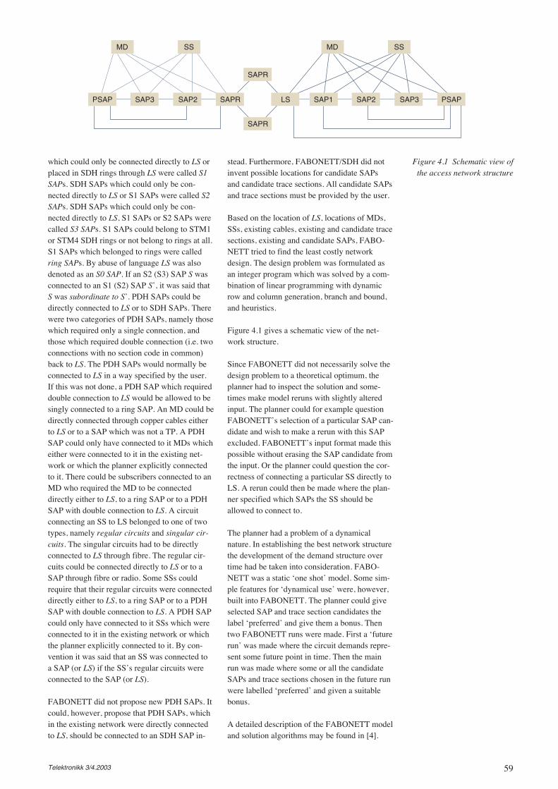
59Telektronikk 3/4.2003
which could only be connected directly to LS orplaced in SDH rings through LS were called S1SAPs. SDH SAPs which could only be con-nected directly to LS or S1 SAPs were called S2SAPs. SDH SAPs which could only be con-nected directly to LS, S1 SAPs or S2 SAPs werecalled S3 SAPs. S1 SAPs could belong to STM1or STM4 SDH rings or not belong to rings at all.S1 SAPs which belonged to rings were calledring SAPs. By abuse of language LS was alsodenoted as an S0 SAP. If an S2 (S3) SAP S wasconnected to an S1 (S2) SAP S’, it was said thatS was subordinate to S’. PDH SAPs could bedirectly connected to LS or to SDH SAPs. Therewere two categories of PDH SAPs, namely thosewhich required only a single connection, andthose which required double connection (i.e. twoconnections with no section code in common)back to LS. The PDH SAPs would normally beconnected to LS in a way specified by the user.If this was not done, a PDH SAP which requireddouble connection to LS would be allowed to besingly connected to a ring SAP. An MD could bedirectly connected through copper cables eitherto LS or to a SAP which was not a TP. A PDHSAP could only have connected to it MDs whicheither were connected to it in the existing net-work or which the planner explicitly connectedto it. There could be subscribers connected to anMD who required the MD to be connecteddirectly either to LS, to a ring SAP or to a PDHSAP with double connection to LS. A circuitconnecting an SS to LS belonged to one of twotypes, namely regular circuits and singular cir-cuits. The singular circuits had to be directlyconnected to LS through fibre. The regular cir-cuits could be connected directly to LS or to aSAP through fibre or radio. Some SSs couldrequire that their regular circuits were connecteddirectly either to LS, to a ring SAP or to a PDHSAP with double connection to LS. A PDH SAPcould only have connected to it SSs which wereconnected to it in the existing network or whichthe planner explicitly connected to it. By con-vention it was said that an SS was connected toa SAP (or LS) if the SS’s regular circuits wereconnected to the SAP (or LS).
FABONETT did not propose new PDH SAPs. Itcould, however, propose that PDH SAPs, whichin the existing network were directly connectedto LS, should be connected to an SDH SAP in-
stead. Furthermore, FABONETT/SDH did notinvent possible locations for candidate SAPsand candidate trace sections. All candidate SAPsand trace sections must be provided by the user.
Based on the location of LS, locations of MDs,SSs, existing cables, existing and candidate tracesections, existing and candidate SAPs, FABO-NETT tried to find the least costly networkdesign. The design problem was formulated asan integer program which was solved by a com-bination of linear programming with dynamicrow and column generation, branch and bound,and heuristics.
Figure 4.1 gives a schematic view of the net-work structure.
Since FABONETT did not necessarily solve thedesign problem to a theoretical optimum, theplanner had to inspect the solution and some-times make model reruns with slightly alteredinput. The planner could for example questionFABONETT’s selection of a particular SAP can-didate and wish to make a rerun with this SAPexcluded. FABONETT’s input format made thispossible without erasing the SAP candidate fromthe input. Or the planner could question the cor-rectness of connecting a particular SS directly toLS. A rerun could then be made where the plan-ner specified which SAPs the SS should beallowed to connect to.
The planner had a problem of a dynamicalnature. In establishing the best network structurethe development of the demand structure overtime had be taken into consideration. FABO-NETT was a static ‘one shot’ model. Some sim-ple features for ‘dynamical use’ were, however,built into FABONETT. The planner could giveselected SAP and trace section candidates thelabel ‘preferred’ and give them a bonus. Thentwo FABONETT runs were made. First a ‘futurerun’ was made where the circuit demands repre-sent some future point in time. Then the mainrun was made where some or all the candidateSAPs and trace sections chosen in the future runwere labelled ‘preferred’ and given a suitablebonus.
A detailed description of the FABONETT modeland solution algorithms may be found in [4].
Figure 4.1 Schematic view ofthe access network structure
MD SS
SAPR
SAPR
PSAP SAP3 SAP2 SAPR
SAPR
SAPR
MD SS
LS SAP1 SAP2 SAP3 PSAP
60 Telektronikk 3/4.2003
5 RUGSAM/RUGINETT/PETRA–Transport Network Planning
Up to the early 1980s the routing and groupingof circuits in what is now called the transportnetwork was done manually. Telenor had experi-mented with the use of planning tools from othertelecommunication administrations withoutmuch success, and it was decided to give Tele-nor R&D the task of developing an optimizationtool. The development of the tool went throughseveral phases. In the first phase routing andgrouping of circuits in a pure PDH network wasconsidered. The tool RUGSAM consisted of twooptimization models where the first model opti-mized routing without considering grouping.Then the model was changed into a singlemodel, RUGINETT, which optimized routingand grouping simultaneously. RUGINETT wasgeneralized to consider a combined PDH andSDH network. In RUGINETT the cable andradio connections were considered as given, andthe tool proposed cost-effective routing andgrouping of demands in the given network.Eventually it was found that this scope was toonarrow, and that the RUGINETT methodologycould be generalized to also propose newtrenches, ducts, cables, and radio connections,and thus become a combined network designand network utilization tool. Even if the basicideas were the same, the generalization was sofundamental that the tool was renamed and wascalled PETRA. PETRA contained an optimiza-tion model based on integer programming whichproposed the installation of new components likemultiplexers, cables and radio connections andring structures, and at the same time how thenetwork should be used to service forecasteddemands. PETRA did not pretend to solve theinteger program to optimality. However, the userinterface allowed the planner to make modifica-tions to the proposed solutions and check feasi-bility and costs.
We shall briefly describe the basic concepts thatwere used in PETRA. The term route objectswere used as a common name for connectionsand equipment. The route objects were parti-tioned into connection objects (short: connec-tions) and equipment objects (short: equipment).Equipment objects were situated in nodes. Everyroute object belonged to a route object type.
Connections were generally routed on other con-nections in the connections hierarchy and possi-bly on nodes according to a set of inputted rout-ing rules. In general, however, existing connec-tions or connections specified by the plannercould have partial routing only, or no routingat all. The routing rules were visualized by anacyclic routing graph. The nodes representedroute objects. An arc from node R to node R’indicated that a route object of type R could be
routed on a route object of type R’. One or moreweight factors could be associated with arc (R,R’) in the graph indicating the fraction of the dif-ferent capacities of type R’ taken up by a routeobject of type R routed on R’.
Connections that service circuit demandsdirectly were called demand connections. Theplanner could specify that demand connectionsassociated with a certain demand could or couldnot be routed on by other connections. If ademand could be routed on, it was denotedaccessible. Otherwise it was denoted inaccessi-ble. Accessible demands were treated in the fol-lowing manner in the optimization module:
• For every accessible demand, one or moreconnections (which might be routed on) with-out routing were established which the opti-mization regarded as existing. Normally noexisting connections were routed on theseconnections, but the planner could specifyany partial use of them.
• Each accessible demand was changed into aninaccessible demand where a possible require-ment for diversified routing was maintained.
• After the optimization (which operated withinaccessible demands only), whatever wasrouted on the accessible connections withoutrouting was shifted over to the connectionswhich covered the created demands.
A connection belonged to exactly one connec-tion type. Typical connection types were
• different variants of 2 Mb groups/circuits• x Mb PDH groups/circuits/transmission
systems• x Mb SDH virtual containers/multiplex
sections/groups/circuits• x Mb SDH ring sections• x Mb WDM groups• cables and radio links• XDSL connections, point-to-multipoint con-
nections, conduits and ducts
A connection could be one-way, two-way orundirected and was characterized by capacities,costs and how it was governed by the routingrules. In particular, one-way connections couldbe routed on one-way, two-way, and undirectedconnections, whilst two-way connections couldbe routed on two-way and undirected connec-tions only, and undirected connections couldbe routed on undirected connections only.
The number of possible connections is huge, andit would be impossible to introduce them all asdecision variables in the optimization. Theywere therefore generated dynamically through
61Telektronikk 3/4.2003
a column generation technique. Another meansof keeping the number of variables down wasto operate with connection sets in lieu of connec-tions, where a connection set was a set of con-nections with identical routing.
The (mixed integer) optimization problem couldin principle be solved to optimality by a branch-and-generate algorithm. However, the very sizeof the problem made this prohibitive, and theproblem was instead solved by a combinationof linear programming and heuristics.
Like the access network planner, the transportnetwork planner had a problem of a dynamicalnature. In establishing the best design, the devel-opment of the demands over time had to be takeninto consideration. Like FABONETT, PETRAwas a static ‘one shot’ model, and the same fea-tures for ‘dynamical use’ were built into PETRA.Two PETRA runs could be made, first a ‘futurerun’ where the demands represent some futurepoint in time, and then a main run where someor all the route objects chosen in the future runcould be labelled ‘preferred’ and given a bonus.
A detailed description of an early version ofRUGINETT may be found in [5].
6 MOBANETT – GSM AccessNetwork Planning
Like for the other networks we have discussed,planners of mobile networks in Telenor hadfound that manual planning of the GSM accessnetwork was time-consuming, and that theywould have capacity for analyzing a few alterna-tives only. Therefore Telenor R&D was againgiven the task of developing a suitable PC-basedplanning tool. The result was the tool MOBA-NETT which attempted to find a GSM accessnetwork which minimized total cost. Like theother tools, MOBANETT did not pretend tosolve the cost minimization problem to optimal-ity. However, the accompanying user interfaceallowed the planner to make modifications to thesolution found by MOBANETT and check feasi-bility and cost.
6.1 GeneralMOBANETT consisted of several moduleswhich could be put into one of two categories:
• optimization modules which found solutionsto the cost minimization problem by mathe-matical and graph teoretical methods;
• modules which enabled the user to interfacewith MOBANETT via (input and output)tables and which prepared the data formatssuitable for the optimization modules.
6.2 The GSM Access NetworkDesign Problem
The mobile subscribers can connect to a set ofgiven Base Transceiver Stations (BTSs).
Several BTSs can be connected together forminga rooted tree. The BTS sitting at the root of sucha tree is called an anchor BTS.
Each anchor BTS must be connected to a BaseStations Controller (BSC), possibly via a DigitalAccess Cross Connect System (DACS). InMOBANETT each BTS is characterized by anumber of 64 kbit/s radio channels. The connec-tion must have sufficient capacity to be able tocarry the total number of radio channels for allBTSs in the rooted tree associated with theanchor BTS.
Each BSC must in turn be connected to a MobileServices Switching Centre (MSC). The connec-tion must have sufficient capacity to carry thetraffic from the BSC subject to a given blockingprobability.
Each MSC must be connected to one or twoMain Switches (FS2s). The connection musthave sufficient capacity to carry the traffic fromthe MSC subject to a given blocking probabilityand a given so-called redundancy factor. Tosimplify the presentation we shall assume thateach MSC should be connected to two FS2s.
An MSC and a BSC can be collocated in orderto reduce cost.
Thus the GSM access network has a tree struc-ture. This structure is shown in Figure 6.1.
6.3 Cost Minimization,General Description
In Figure 6.1 the network to be designed liesbetween the two horizontal lines.
The locations of the FS2s and the BTSs and thenumber of radio channels between the anchorBTSs and the BSC/DACS were input to MOBA-NETT. MOBANETT tried to determine
• where MSCs, BSCs and DACSs should beplaced;
• which BTSs should be connected to whichDACS/BSCs;
• which BSCs should be connected to whichMSCs;
in order to obtain a feasible access network atthe lowest possible cost.
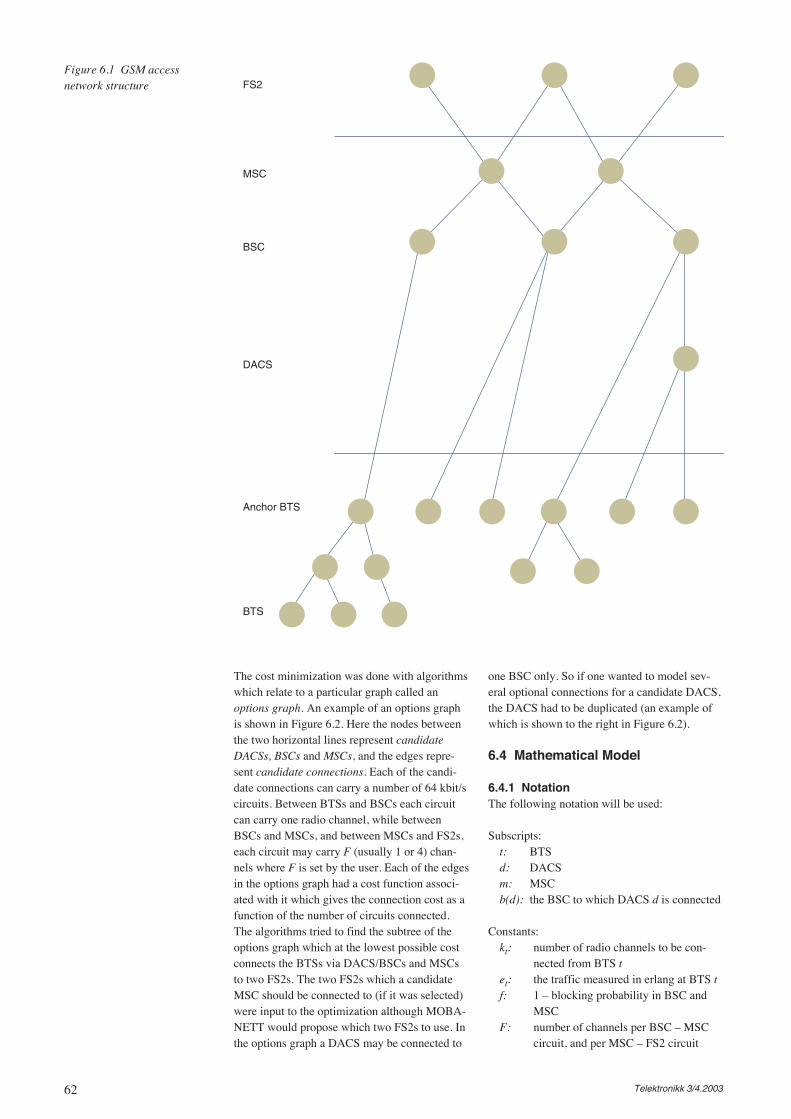
62 Telektronikk 3/4.2003
The cost minimization was done with algorithmswhich relate to a particular graph called anoptions graph. An example of an options graphis shown in Figure 6.2. Here the nodes betweenthe two horizontal lines represent candidateDACSs, BSCs and MSCs, and the edges repre-sent candidate connections. Each of the candi-date connections can carry a number of 64 kbit/scircuits. Between BTSs and BSCs each circuitcan carry one radio channel, while betweenBSCs and MSCs, and between MSCs and FS2s,each circuit may carry F (usually 1 or 4) chan-nels where F is set by the user. Each of the edgesin the options graph had a cost function associ-ated with it which gives the connection cost as afunction of the number of circuits connected.The algorithms tried to find the subtree of theoptions graph which at the lowest possible costconnects the BTSs via DACS/BSCs and MSCsto two FS2s. The two FS2s which a candidateMSC should be connected to (if it was selected)were input to the optimization although MOBA-NETT would propose which two FS2s to use. Inthe options graph a DACS may be connected to
one BSC only. So if one wanted to model sev-eral optional connections for a candidate DACS,the DACS had to be duplicated (an example ofwhich is shown to the right in Figure 6.2).
6.4 Mathematical Model
6.4.1 NotationThe following notation will be used:
Subscripts:t: BTSd: DACSm: MSCb(d): the BSC to which DACS d is connected
Constants:kt: number of radio channels to be con-
nected from BTS tet: the traffic measured in erlang at BTS tf: 1 – blocking probability in BSC and
MSCF: number of channels per BSC – MSC
circuit, and per MSC – FS2 circuit
Figure 6.1 GSM accessnetwork structure FS2
MSC
BSC
DACS
Anchor BTS
BTS
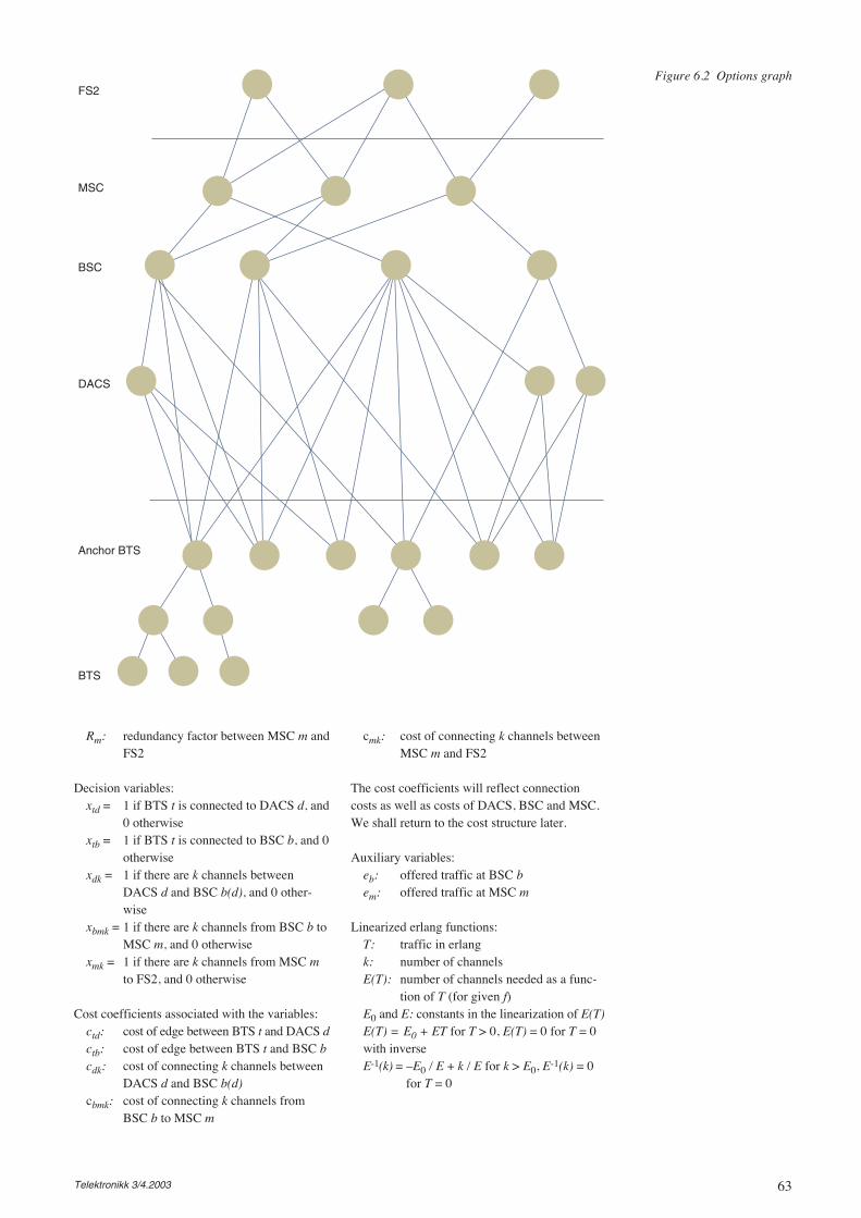
63Telektronikk 3/4.2003
Rm: redundancy factor between MSC m andFS2
Decision variables:xtd = 1 if BTS t is connected to DACS d, and
0 otherwisextb = 1 if BTS t is connected to BSC b, and 0
otherwisexdk = 1 if there are k channels between
DACS d and BSC b(d), and 0 other-wise
xbmk = 1 if there are k channels from BSC b toMSC m, and 0 otherwise
xmk = 1 if there are k channels from MSC mto FS2, and 0 otherwise
Cost coefficients associated with the variables:ctd: cost of edge between BTS t and DACS dctb: cost of edge between BTS t and BSC bcdk: cost of connecting k channels between
DACS d and BSC b(d)cbmk: cost of connecting k channels from
BSC b to MSC m
cmk: cost of connecting k channels betweenMSC m and FS2
The cost coefficients will reflect connectioncosts as well as costs of DACS, BSC and MSC.We shall return to the cost structure later.
Auxiliary variables:eb: offered traffic at BSC bem: offered traffic at MSC m
Linearized erlang functions:T: traffic in erlangk: number of channelsE(T): number of channels needed as a func-
tion of T (for given f)E0 and E: constants in the linearization of E(T)E(T) = E0 + ET for T > 0, E(T) = 0 for T = 0with inverseE-1(k) = –E0 / E + k / E for k > E0, E-1(k) = 0
for T = 0
Figure 6.2 Options graphFS2
MSC
BSC
DACS
Anchor BTS
BTS
64 Telektronikk 3/4.2003
6.4.2 Optimization ModelThe cost minimization problem was formulatedas follows:
minimize Σctdxtd + Σctbxtb + Σcdkxdk +Σcbmkxbmk + Σcmkxmk
subject to
Σtktxtd ″ Σkkxdk (balance in DACS d) (6.1)
E(eb) ″ FΣmkkxbmk (balance in BSC b) (6.2)
RmE(em) ″ Σkkxmk (balance in MSC m) (6.3)
where
eb = Σt,d∈betxtd + Σtetxtb
and
em = ΣbfE-1 (FΣkkxbmk)
Using the formulas for E(T) and E-1(k) trans-forms (2) and (3) to (4) and (5):
E Σt,d∈betxtd + EΣtetxtb ″ Σmk(Fk – E0)xbmk(6.4)
RmfΣbk(Fk – E0)xbmk ″ Σk(k – RmE0)xmk (6.5)
Note that we must have k ≥ E0 / F in BSCs andk ≥ RmE0 in MSCs. This defines the minimalvalues kmin which k can take.
Thus the optimization model becomes:
minimize Σctdxtd + Σctbxtb + Σcdkxdk +Σcbmkxbmk + Σcmkxmk
subject to
Σtktxtd ″ Σkkxdk (balance in DACS d) (6.6)
E Σt,d∈betxtd + EΣtetxtb ″ Σmk(Fk – E0)xbmk
(balance in BSC b) (6.7)
RmfΣbk(Fk – E0)xbmk ″ Σk(k – RmE0)xmk
(balance in MSC m) (6.8)
where
k ≥ E0 / F in BSCs and k ≥ RmE0 in MSCs.
6.5 Cost StructureA detailed presentation of the cost elementswhich the planner gives via tables to MOBA-NETT is not given here. Prior to the optimiza-tion the costs of components (DACS, BSC,MSC) and connections as a function of the num-ber of radio channels c were approximated byfunctions C(c) which in general were sums ofup to three terms. These terms were
a constant part = C,a linear part Lc, anda ‘saw tooth’ part T(c) = T . (1 – c(mod 30) / c)
Thus C(c) = C + Lc + T(c).
The saw tooth part reflected cost elements whichdepended on the number of 2 Mbit/s circuits.
We shall now describe the individual cost func-tions and how they were allocated to the edgesin the options graph.
6.5.1 DACS CostThe cost of a DACS consisted of a cost per2 Mbit/s circuit connected to a BTS or a BSC.The cost decomposed into a linear part and asaw tooth part. The linear part translated into aconstant part which was put on each of the edgesconnecting to BTSs. The saw tooth part was puton the edge connecting to the BSC.
6.5.2 BSC CostThe cost of a BSC consists of a fixed cost plusa cost per radio channel coming from the BTSswhich are connected to it (possibly via DACS).The cost decomposed into a constant part anda linear part. The constant part was put on theedges connecting to MSCs. The linear part trans-lated into constant parts on the edges betweenBTSs and the BSC and on the edges betweenBTSs and the DACSs associated with the BSC.
6.5.3 MSC CostThe cost of an MSC consisted of a fixed costplus a cost per 2 Mbit/s circuit connecting to aBSC or FS2. The cost decomposed into a con-stant part on the edges to the FS2s, a linear parton the edges to the BSCs, a saw tooth part oneach of the edges to BSCs and a saw tooth partfor each of the edges to FS2s.
6.5.4 Cost of Connection Between BTSand DACS/BSC
The cost of the connection between a BTS anda DACS/BSC consisted of a cost per 64 kbit/s orper 2 Mbit/s. In both cases this translated into aconstant cost on the edge between the BTS andDACS.
6.5.5 Cost of Connection Between DACSand BSC
The cost of the connection between a DACSand a BSC consisted of a cost per 2 Mbit/s. Thisdecomposed into a linear part which translatesinto constant parts on the BTS – DACS edgesand a saw tooth part on the DACS – BSC edge.
6.5.6 Cost of Connection Between BSCand MSC
The cost of the connection between a BSC andan MSC consisted of a cost per 2 Mbit/s. This

65Telektronikk 3/4.2003
decomposed into a linear part which translatedinto linear parts and saw tooth parts on the BSC– MSC edges.
6.5.7 Cost of Connection Between MSCand FS2
The cost of the connection between an MSC andan FS2 consisted of a cost per 2 Mbit/s. Thisdecomposed into a linear part which translatedinto a linear part and a saw tooth part on theMSC – FS2 edge.
6.5.8 Collocation of BSC and MSCIt could be cost effective to place a BSC and anMSC in the same node. This was treated simplyby introducing into the options graph additionalnodes for a candidate MSC and a candidate BSCwith reduced costs and a zero cost connectionbetween them.
6.5.9 Shifting Linear Edge CostsTowards BTS
It was believed that the optimization algorithmsfunction better if the cost elements were shiftedto edges in the options graph which are as closeto the BTSs as possible. We shall now describehow this shifting is done in principle.
We have already seen how linear costs associ-ated with connections between DACS and BSCwere changed to constant costs on DACS – BTSedges. We similarly translated the linear costs onthe FS2 – MSC edges to corresponding MSC –BSC edges. In order to do this it was necessaryto find the number k of channels between FS2sand an MSC as a function of the number k’ ofchannels between the MSC and MSCs. Inequal-ity (6.5), which could just as well have beenwritten as an equality, gives
RmfΣb(Fk’ – E0) = k – RmE0 (6.9)
where the sum is over the BSCs connected to theMSC.
This gives
k = RmE0 + Σb(RmfFk’ – RmfE0) (6.10)
A linear term Lc on the edge MSC – FS2 thustranslates into
a constant term –LRmfE0 on each BSC – MSCedge
a linear term LRmfFk’ on each BSC – MSCedge
a constant term LRmE0 on the FS2 – MSCedge
Linear costs on the edges between MSCs andBSCs cannot be moved towards the DACS/BTSsin the same way because a BSC can be con-nected to several alternative MSCs. The best wecan do is for a BSC to move a part of each linearMSC – BSC cost equal to the minimal linearMSC – BSC cost for this BSC. This was doneafter all other costs had been allocated and pos-sibly shifted. Let Lmin be the minimal coefficientfor the linear costs on the edges from MSCs andlet L be the corresponding coefficient for the edgeto an arbitrary MSC. The linear cost coefficienton the BSC – MSC edge was changed to L – Lmin.
Considerations analogous to those above givethe number k of channels between BSC andMSC equal to
k = E0 / F + EΣt,d∈bet / F + EΣtet / F.
The cost shifting thus resulted in
a constant term LminEet / F on each BTS –DACS edge
a constant term LminEet / F on each BTS –BSC edge
a constant term LminE0 / F on each BTS –DACS edge
a linear term (L – Lmin)k on the BSC – MSCedge
6.6 Candidate BSC and MSC Nodesand Connections
In order to relieve the planner of the tedious taskof inputting all locations for candidate BSClocations a simple algorithm was developedwhich proposed candidate BSC nodes.
The geographical locations of the BTSs andFS2s were given as input to MOBANETT. Inaddition it was possible to give as input the loca-tions of NMT base stations and NMT switches(MTXs). All these geographical points had thepossibility of becoming candidate BSC nodes.
The MTXs were automatically made into candi-date BSC nodes, and the planner would add onmore candidate BSC nodes of his choice. There-after he could apply the algorithm below.
Algorithm which proposes additionalcandidate BSC nodes:
1 Draw the largest circle possible around everycandidate node (with the node as centre) so thatthe total traffic generated by the BTSs in thecircle is below a given limit (the exclusionlimit), and exclude all points in the circles fromthe possibility of becoming candidate nodes.
66 Telektronikk 3/4.2003
2 If every geographical point is either a candi-date node or excluded, stop. Otherwise drawthe largest possible circle around every geo-graphical point (with the point as centre)which is not yet a candidate node and whichis not yet excluded, so that the total trafficgenerated by the BTSs in the circle is belowa given limit (the inclusion limit). Define thepoint with the smallest circle as a candidateBSC node. Go to 1.
After the candidate BSC nodes had been decidedupon the planner selected a subset of these, pos-sibly augmented by some other geographicalpoints, as candidate MSC nodes.
The planner could also get some assistance insetting up candidate connections. MOBANETTwould for every MSC candidate propose connec-tions to the two closest FS2s and to the closestcandidate BSC nodes up to a given number andwithin a certain distance. Furthermore MOBA-NETT would for each candidate BSC proposeconnections to the closest BTSs up to a givennumber and within a given distance. Connec-tions via DACS were also proposed according tocertain criteria which we shall not go into here.
6.7 Solving the Optimization Model
6.7.1 Use of Lagrange RelaxationThe optimization model as defined in 3.2 wassolved by using Lagrange relaxation and subgra-dient optimization. The technicalities connectedwith the use of the subgradient method are stan-dard and will not be described here. Inequalities(1), (4) and (5) were relaxed. However, the con-dition that the BTSs must be connected to FS2sin a tree structure was retained as a constraint.The relaxed problem thus became a classicalSteiner problem in a rooted directed acyclicgraph. The root node was an auxiliary node con-nected to the candidate MSC nodes where thecost of the connection reflected the cost of con-necting the MSC to its two FS2s, and where thespecial nodes to be connected to the root repre-sented the BTSs.
6.7.2 Solving the Steiner SubproblemSince the Steiner subproblem had to be solved asubstantial number of times a heuristic is used.The heuristic chosen was Wong’s dual ascentalgorithm [2] followed by Pacheco-Maculan’ssolution improvement algorithm [3], both spe-cialized to rooted directed acyclic graphs.
7 GSM Frequency Planningby MOBINETT
The requirements for GSM services increasedrapidly in the early 1990s, and it was realizedthat it was crucial to have access to a good PC-based tool for frequency planning. Telenor R&D
had earlier experimented with algorithms forfinding the least number of frequencies neces-sary to carry a given traffic in a network with agiven set of BTSs with sufficiently low level ofinterference. Telenor R&D was then given thetask of instead making an optimization toolwhich assigned a given number of frequencies toeach BTS such that the level of interference wasacceptable and minimized. The input was a setof admissible frequencies (which needed notbe contiguous) and a symmetric compatibilitymatrix which for each pair of BTSs indicatedwhether they interfered on neighboring frequen-cies, on same frequencies only, or not at all.MOBINETT went through several stages.
The first variant considered only BTSs whichsupported neither baseband nor synthesizer hop-ping. This problem was formulated as a pureinteger programming problem which was ini-tially solved by a combination of linear pro-gramming and heuristics. For realistic cases thenumber of variables was reasonably small (about10,000) whilst the number of constraints couldbe rather large (> 150,000). Since the linear pro-gramming software we used performed betterwith a high number of variables and a low num-ber of constraints than vice versa, the transposedproblem (where the dual variables had to be inte-gers) was solved instead. In order to solve theproblem to optimality the heuristic was replacedby a dual ‘branch and cut and generate’ softwarepackage that was designed and implemented atTelenor R&D.
As new BTSs which supported baseband andsynthesizer hopping became available, MOBI-NETT had to be modified accordingly. The com-patibility matrix was replaced by two asymmet-ric interference matrices, one describing interfer-ences from interfering BTSs to victim BTSs onthe same frequency, and one describing corre-sponding interferences on neighboring frequen-cies. Thresholds were set for acceptable interfer-ence. This necessitated a complete remodelingof the problem, and new solution algorithms hadto be implemented. The new MOBINETT triedto allocate frequencies to cells such that the fre-quency requirements were satisfied and such thata weighted sum of interference contributionsabove given thresholds were minimized.
The planner could partition the cells into subsetsand solve the allocation problem for one subsetat a time. The basic approach was to formulatethe subproblems as integer programs which wassolved by classical branch and bound. In addi-tion, postprocessors based on tabu search andsimulated annealing were implemented. MOBI-NETT is at the time of writing still in use.

67Telektronikk 3/4.2003
8 ConclusionWe see that Telenor R&D over the years hasbeen involved in the establishment of networkplanning tools for most parts of the physical net-work. This had not been possible without theparticipation and support from dedicated net-work planners in Telenor. The main hurdleshave been:
• The varying quality of the data in the networkdatabases. A spin-off effect of the planningtool development has been a substantial in-crease in the accuracy of some of the datasources.
• The responsibility for the planning of the dif-ferent networks was in the past decentralized.The local planners had a variety of responsi-bilities, and it was often difficult for them toallocate the time necessary to acquire andmaintain the necessary familiarity with thetools. Also, the ICT equipment available tothe planners at the local level was not alwayssufficient for making effective use of the tools.
There are reasons to believe that these hurdleswill be easier to overcome in the future:
• The requirement for high accuracy in the net-work databases is becoming more and morepronounced, not only because of requirementsfrom planning tools.
• There is a tendency to centralize the networkplanning activity. This implies that plannerscan dedicate more of their time to get the mostout of sophisticated planning tools.
• The reliability, capacity and speed of ICTequipment has become more than sufficient tosupport the optimization algorithms that formthe motor in modern network planning tools.
Finally it should be observed that the develop-ment, implementation, and use of network plan-ning tools ought to be an ongoing process. Boththe demands for new services and the technol-ogy that can be used to serve them evolve atincreasing speed.
9 References1 Rayward-Smith, V J, Clare, A. On Finding
Steiner Vertices. Networks, 16, 283–294,1986.
2 Wong, R T. A Dual Ascent Approach forSteiner Tree Problems on a Directed Graph.Mathematical Programming, 28, 271–287,1984.
3 Pacheco, O I P, Maculan, N. Metodo Heuris-tic para o Problema de Steiner num GrafoDirecionado. Proceedings of the III CLAIO,Santiago, Chile, August 1986.
4 Lorentzen, R. Mathematical Model andAlgorithms for FABONETT/SDH. Telek-tronikk, 94 (1), 135–145, 1998.
5 Lorentzen, R. Mathematical Methods andAlgorithms in the Network Utilization Plan-ning Tool RUGINETT. Telektronikk, 90 (4),73–82, 1994.
Telektronikk 3/4.2003
1 IntroductionIn today’s world, change and uncertainty seemto be constants. On the one hand this is nice, asimprovements are captured in the evolution pro-cess. On the other hand, the ongoing dynamicsis hard to capture in network planning with alonger time horizon. In fact, a claim could bethat there is no point at all in looking a few yearsahead as for (almost) certain, the future will notbe exactly as predicted. It is fair to say that thisclaim is missing the main objectives of carryingout strategic planning, for networks as well asfor other areas. Besides being incorrect, theclaim disregards the benefits following from asystematic analysis of a company’s surroundingsand future options.
A motivation for evaluating the coming avail-able choices is to use the results to elaborate arobust action plan to cover triggers for makingdecisions or to initiate actions as well as optionalactions. As described later a robust plan supportsa flexible roadmap of system/network evolution,that is what to do for each of the systems givencertain factors. Hence, a consequence of this isto try to postpone final decisions until theactions have to be started. This gives the optionto not start the action or carry out another action.
In an economic sense, there are at least twomotivations why flexibility should be includedin an investment evaluation: Firstly, the estimateof the activity value is improved, better reflect-ing the actual characteristics of the challenge.Another motivation is the improved insightgained for uncertainties and hence a betterunderstanding of the flexibility and the optionsexpected. Commonly real options are applied toinclude these options in the evaluation. Bringingreal options into the equation increases the levelof activity values, although the increase differsfor the different nature of activities.
The following sections give an overall descrip-tion of strategy work, both the intention (Section2) and the overall approach (Section 3). A num-ber of criteria are needed to choose between the
different options, as elaborated in Section 4. Aspresented in Section 5, a sound strategy mustalso relate to trends at various levels. Section 6presents how scenario work can be applied inorder to assist when deriving strategies, followedby examples in Section 7. A quantitativeapproach is then given in Section 8. Assessingrisk is also an essential element in any strategyas described in Section 9. Some overall discus-sions are then given in the last two sections.
2 Relating Long and ShortTerm – the Scope and theChallenges
It is fundamental to understand that the strategicevaluations and planning are not carried out fortheir own purposes per se, but need to be relatedto the current situation in order to get practicalimplications. Naturally a number of steps in thestrategy can be located some time ahead, andhence do not necessarily influence today’s activ-ities. This means that one result is to sort out thedecisions to be made in a timely manner. How-ever, one main result is to devise the actionsneeded in the actual situation an actor finds itselfin. The overall process is depicted in Figure 1.
A number of general steps can be identified:
i. The “frame” of the task is described by theelements: a) Current network portfolio, b)Forecasts and trends, c) Set of (optional) tar-get states. Naturally, these are interrelated asa potential target state is influenced by one’sposition in the existing situation and a sce-nario for further development. That is, a sce-nario-based approach will likely apply forthis step. Included in the current portfoliogoes also an assessment of short-term devel-opment, e.g. given through a “historic”description in the traffic/user developmentin a system.
ii. The “gap” between the current situation andthe target states is explained with a set ofpossible paths. That is, a path will tell a storyfor how the current network portfolio will
Network Strategy StudiesT E R J E J E N S E N
Every network operator needs to have a network strategy covering the complete network portfolio. The
strategy must also be operational, meaning to be related to decisions and actions in near-time. One
main goal for having a strategy is to be prepared for chances that can be revealed with time. That is,
the strategy is likely to assist in detecting business opportunities.
A number of methods can be applied when elaborating the strategy, including scenarios, cost/benefit
calculations and risk assessment – these aspects are briefly presented in this article.
Dr. Terje Jensen (41) isResearch Manager at TelenorResearch and Development. Inrecent years he has mostly beenengaged in network strategystudies addressing the overallnetwork portfolio of an operator.Besides these activities he hasbeen involved in internal andinternational projects on networkplanning, performance model-ling/analyses and dimensioning.
68
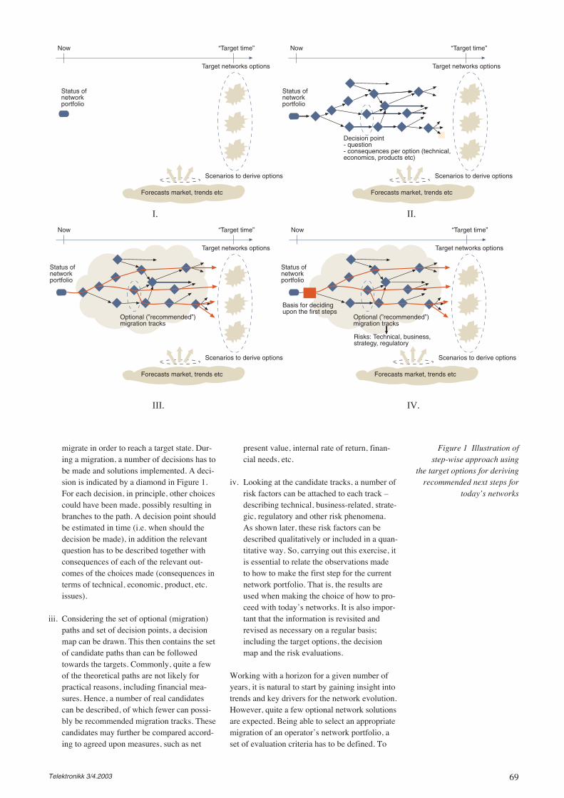
69Telektronikk 3/4.2003
migrate in order to reach a target state. Dur-ing a migration, a number of decisions has tobe made and solutions implemented. A deci-sion is indicated by a diamond in Figure 1.For each decision, in principle, other choicescould have been made, possibly resulting inbranches to the path. A decision point shouldbe estimated in time (i.e. when should thedecision be made), in addition the relevantquestion has to be described together withconsequences of each of the relevant out-comes of the choices made (consequences interms of technical, economic, product, etc.issues).
iii. Considering the set of optional (migration)paths and set of decision points, a decisionmap can be drawn. This then contains the setof candidate paths than can be followedtowards the targets. Commonly, quite a fewof the theoretical paths are not likely forpractical reasons, including financial mea-sures. Hence, a number of real candidatescan be described, of which fewer can possi-bly be recommended migration tracks. Thesecandidates may further be compared accord-ing to agreed upon measures, such as net
present value, internal rate of return, finan-cial needs, etc.
iv. Looking at the candidate tracks, a number ofrisk factors can be attached to each track –describing technical, business-related, strate-gic, regulatory and other risk phenomena.As shown later, these risk factors can bedescribed qualitatively or included in a quan-titative way. So, carrying out this exercise, itis essential to relate the observations madeto how to make the first step for the currentnetwork portfolio. That is, the results areused when making the choice of how to pro-ceed with today’s networks. It is also impor-tant that the information is revisited andrevised as necessary on a regular basis;including the target options, the decisionmap and the risk evaluations.
Working with a horizon for a given number ofyears, it is natural to start by gaining insight intotrends and key drivers for the network evolution.However, quite a few optional network solutionsare expected. Being able to select an appropriatemigration of an operator’s network portfolio, aset of evaluation criteria has to be defined. To
Figure 1 Illustration ofstep-wise approach using
the target options for derivingrecommended next steps for
today’s networks
Now “Target time”
Target networks options
Scenarios to derive options
Forecasts market, trends etc
Now “Target time”
Target networks options
Scenarios to derive options
Forecasts market, trends etc
Status ofnetworkportfolio
Decision point- question- consequences per option (technical,economics, products etc)
Now “Target time”
Target networks options
Scenarios to derive options
Forecasts market, trends etc
Status ofnetworkportfolio
Status ofnetworkportfolio
Optional (”recommended”)migration tracks
Now “Target time”
Target networks options
Scenarios to derive options
Forecasts market, trends etc
Status ofnetworkportfolio
Optional (”recommended”)migration tracks
I. II.
Risks: Technical, business,strategy, regulatory
III. IV.
Basis for decidingupon the first steps
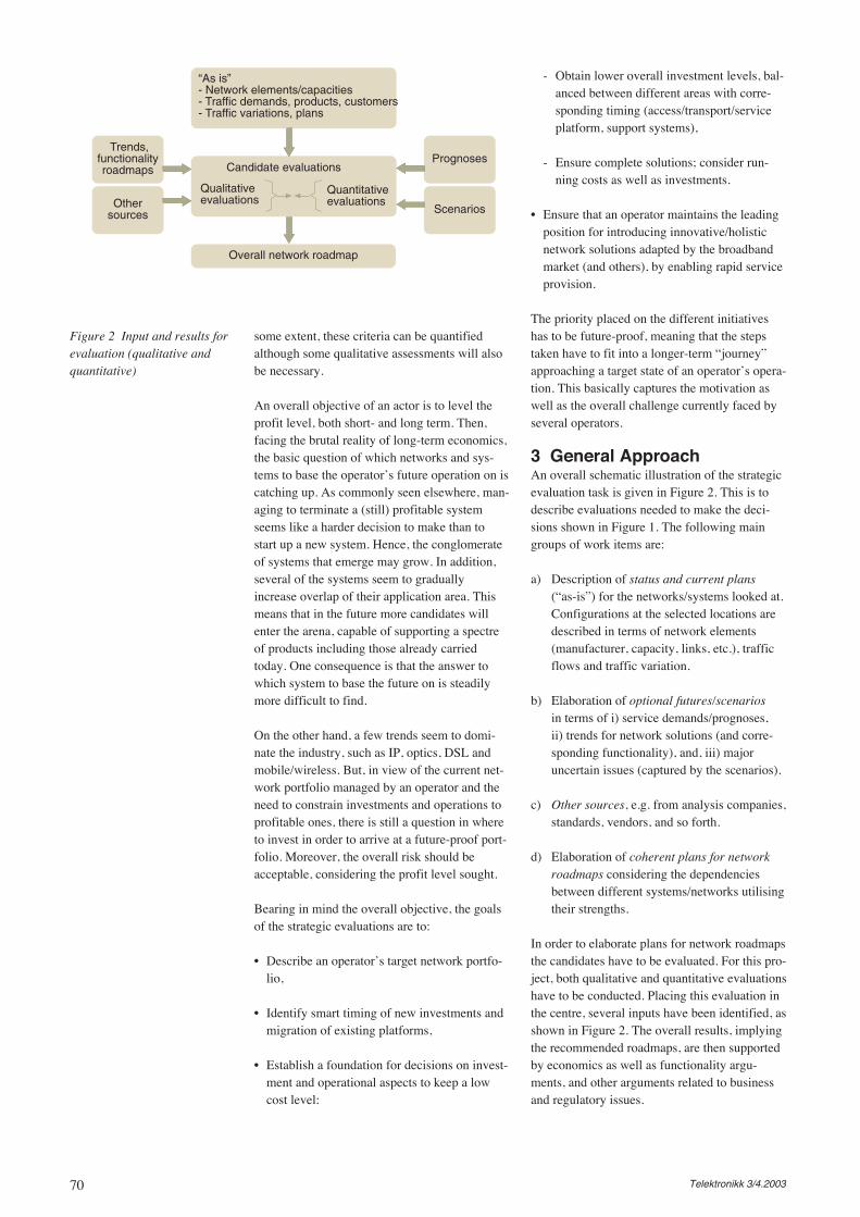
70 Telektronikk 3/4.2003
some extent, these criteria can be quantifiedalthough some qualitative assessments will alsobe necessary.
An overall objective of an actor is to level theprofit level, both short- and long term. Then,facing the brutal reality of long-term economics,the basic question of which networks and sys-tems to base the operator’s future operation on iscatching up. As commonly seen elsewhere, man-aging to terminate a (still) profitable systemseems like a harder decision to make than tostart up a new system. Hence, the conglomerateof systems that emerge may grow. In addition,several of the systems seem to graduallyincrease overlap of their application area. Thismeans that in the future more candidates willenter the arena, capable of supporting a spectreof products including those already carriedtoday. One consequence is that the answer towhich system to base the future on is steadilymore difficult to find.
On the other hand, a few trends seem to domi-nate the industry, such as IP, optics, DSL andmobile/wireless. But, in view of the current net-work portfolio managed by an operator and theneed to constrain investments and operations toprofitable ones, there is still a question in whereto invest in order to arrive at a future-proof port-folio. Moreover, the overall risk should beacceptable, considering the profit level sought.
Bearing in mind the overall objective, the goalsof the strategic evaluations are to:
• Describe an operator’s target network portfo-lio,
• Identify smart timing of new investments andmigration of existing platforms,
• Establish a foundation for decisions on invest-ment and operational aspects to keep a lowcost level:
- Obtain lower overall investment levels, bal-anced between different areas with corre-sponding timing (access/transport/serviceplatform, support systems),
- Ensure complete solutions; consider run-ning costs as well as investments.
• Ensure that an operator maintains the leadingposition for introducing innovative/holisticnetwork solutions adapted by the broadbandmarket (and others), by enabling rapid serviceprovision.
The priority placed on the different initiativeshas to be future-proof, meaning that the stepstaken have to fit into a longer-term “journey”approaching a target state of an operator’s opera-tion. This basically captures the motivation aswell as the overall challenge currently faced byseveral operators.
3 General ApproachAn overall schematic illustration of the strategicevaluation task is given in Figure 2. This is todescribe evaluations needed to make the deci-sions shown in Figure 1. The following maingroups of work items are:
a) Description of status and current plans(“as-is”) for the networks/systems looked at.Configurations at the selected locations aredescribed in terms of network elements(manufacturer, capacity, links, etc.), trafficflows and traffic variation.
b) Elaboration of optional futures/scenariosin terms of i) service demands/prognoses,ii) trends for network solutions (and corre-sponding functionality), and, iii) majoruncertain issues (captured by the scenarios).
c) Other sources, e.g. from analysis companies,standards, vendors, and so forth.
d) Elaboration of coherent plans for networkroadmaps considering the dependenciesbetween different systems/networks utilisingtheir strengths.
In order to elaborate plans for network roadmapsthe candidates have to be evaluated. For this pro-ject, both qualitative and quantitative evaluationshave to be conducted. Placing this evaluation inthe centre, several inputs have been identified, asshown in Figure 2. The overall results, implyingthe recommended roadmaps, are then supportedby economics as well as functionality argu-ments, and other arguments related to businessand regulatory issues.
Figure 2 Input and results forevaluation (qualitative andquantitative)
Trends,functionalityroadmaps Candidate evaluations
Qualitativeevaluations
Quantitativeevaluations
Overall network roadmap
“As is”- Network elements/capacities- Traffic demands, products, customers- Traffic variations, plans
Othersources
Prognoses
Scenarios

71Telektronikk 3/4.2003
4 Criteria for SelectingMigration Branches
4.1 Overall – FinancialIn detailing future network candidates, a numberof options are revealed in terms of choosingwhich candidates to base a further networkmigration on. Hence, there is a need to definea set of criteria to use when selecting whichoptions are the better ones. Some criteria aredescribed in the following.
One basic criterion is the profit levels expectedby taking certain steps. Requirements on the ex-pected profit are given considering the accompa-nying risk level. Hence, higher risk would likelyask for a higher profit level than a lower riskaction. Profit can be estimated in different ways.For example, assuming that network solution isirrelevant to income level, the cost of the solu-tion is to be minimised. In general, however,various solutions may support different levels ofservice and product type. The income side musttherefore also be considered in the equation.
A fundamental challenge on the income side isthat the price level is influenced by many factorsoutside the operator considered, such as com-petitors and regulator. Theoretical models andanalyses exist for similar configurations and willnot be dealt with in this article.
Concerning financial aspects a number of topicsshould be looked at, such as:
• Financing needs, e.g. peak funding,
• Value and profitability evaluations, e.g. netpresent value, internal return rate, paybacktime,
• Sensitivity analyses of major factors.
As for risks, the technology risk addresses onearea. However, a number of additional areascould also be treated:
• Political and market economic risk
• Market and commercial risk (including regu-latory)
• Partner risk (also including vendors)
• Financial risk
• Organisational risk (to follow the activitiesand realise profits)
In order to realise the profit, appropriate stepshave to be prepared for in a timely manner, likeorganisational efficiency, increased revenue,reduced cost, etc. Moreover, exit strategies haveto be elaborated to cover alternative steps/pathsto follow in case some of the planned steps turnout to be unwanted later on in the process.Which exit strategies that are possible shouldalso be discussed. This corresponds with themap of decision points shown in Figure 1.
The interplay with vendors and customers mustalso be obeyed. That is, trends among the usershave to be observed and possibly matched inorder to increase the service demands. Likewise,choices and prioritisations made by the vendorshave to be followed, as it could turn out verycostly to install and maintain a system from avendor that is leaving the market or decides notto support that system in the future.
Keeping in mind the broader set of criteria, afew criteria groups are treated in the following(Figure 3):
• Product-related: capabilities of supporting rel-evant products,
Figure 3 Selectedcriteria classes
Cost-related
Coordination-related
What are others (vendors, competitors etc) doing?
Ris
ks,
Fle
xibi
lity
(”ex
it op
tions
”)
Product-related
Regulatory-related
Profit
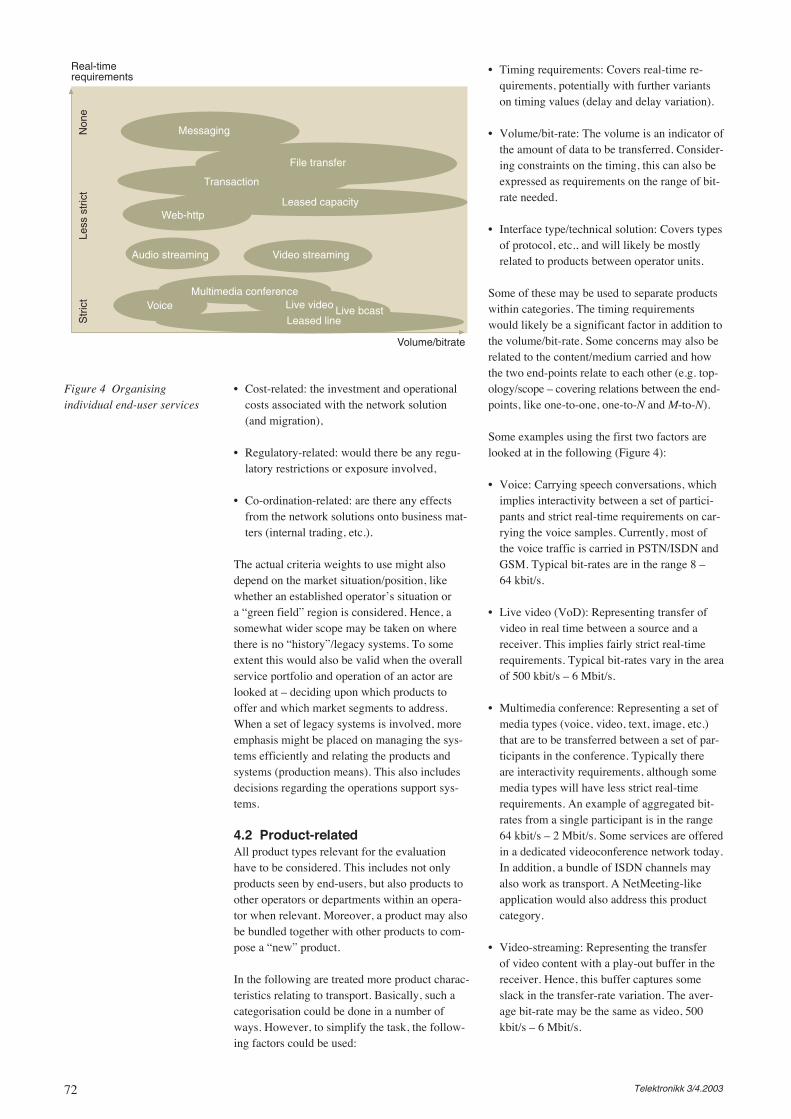
72 Telektronikk 3/4.2003
• Cost-related: the investment and operationalcosts associated with the network solution(and migration),
• Regulatory-related: would there be any regu-latory restrictions or exposure involved,
• Co-ordination-related: are there any effectsfrom the network solutions onto business mat-ters (internal trading, etc.).
The actual criteria weights to use might alsodepend on the market situation/position, likewhether an established operator’s situation ora “green field” region is considered. Hence, asomewhat wider scope may be taken on wherethere is no “history”/legacy systems. To someextent this would also be valid when the overallservice portfolio and operation of an actor arelooked at – deciding upon which products tooffer and which market segments to address.When a set of legacy systems is involved, moreemphasis might be placed on managing the sys-tems efficiently and relating the products andsystems (production means). This also includesdecisions regarding the operations support sys-tems.
4.2 Product-relatedAll product types relevant for the evaluationhave to be considered. This includes not onlyproducts seen by end-users, but also products toother operators or departments within an opera-tor when relevant. Moreover, a product may alsobe bundled together with other products to com-pose a “new” product.
In the following are treated more product charac-teristics relating to transport. Basically, such acategorisation could be done in a number ofways. However, to simplify the task, the follow-ing factors could be used:
• Timing requirements: Covers real-time re-quirements, potentially with further variantson timing values (delay and delay variation).
• Volume/bit-rate: The volume is an indicator ofthe amount of data to be transferred. Consider-ing constraints on the timing, this can also beexpressed as requirements on the range of bit-rate needed.
• Interface type/technical solution: Covers typesof protocol, etc., and will likely be mostlyrelated to products between operator units.
Some of these may be used to separate productswithin categories. The timing requirementswould likely be a significant factor in addition tothe volume/bit-rate. Some concerns may also berelated to the content/medium carried and howthe two end-points relate to each other (e.g. top-ology/scope – covering relations between the end-points, like one-to-one, one-to-N and M-to-N).
Some examples using the first two factors arelooked at in the following (Figure 4):
• Voice: Carrying speech conversations, whichimplies interactivity between a set of partici-pants and strict real-time requirements on car-rying the voice samples. Currently, most ofthe voice traffic is carried in PSTN/ISDN andGSM. Typical bit-rates are in the range 8 –64 kbit/s.
• Live video (VoD): Representing transfer ofvideo in real time between a source and areceiver. This implies fairly strict real-timerequirements. Typical bit-rates vary in the areaof 500 kbit/s – 6 Mbit/s.
• Multimedia conference: Representing a set ofmedia types (voice, video, text, image, etc.)that are to be transferred between a set of par-ticipants in the conference. Typically thereare interactivity requirements, although somemedia types will have less strict real-timerequirements. An example of aggregated bit-rates from a single participant is in the range64 kbit/s – 2 Mbit/s. Some services are offeredin a dedicated videoconference network today.In addition, a bundle of ISDN channels mayalso work as transport. A NetMeeting-likeapplication would also address this productcategory.
• Video-streaming: Representing the transferof video content with a play-out buffer in thereceiver. Hence, this buffer captures someslack in the transfer-rate variation. The aver-age bit-rate may be the same as video, 500kbit/s – 6 Mbit/s.
Figure 4 Organisingindividual end-user services
Messaging
File transfer
Transaction
Leased capacityWeb-http
Video streamingAudio streaming
Multimedia conferenceVoice Live video Live bcast
Leased line
Volume/bitrate
Real-timerequirements
Str
ict
Less
str
ict
Non
e
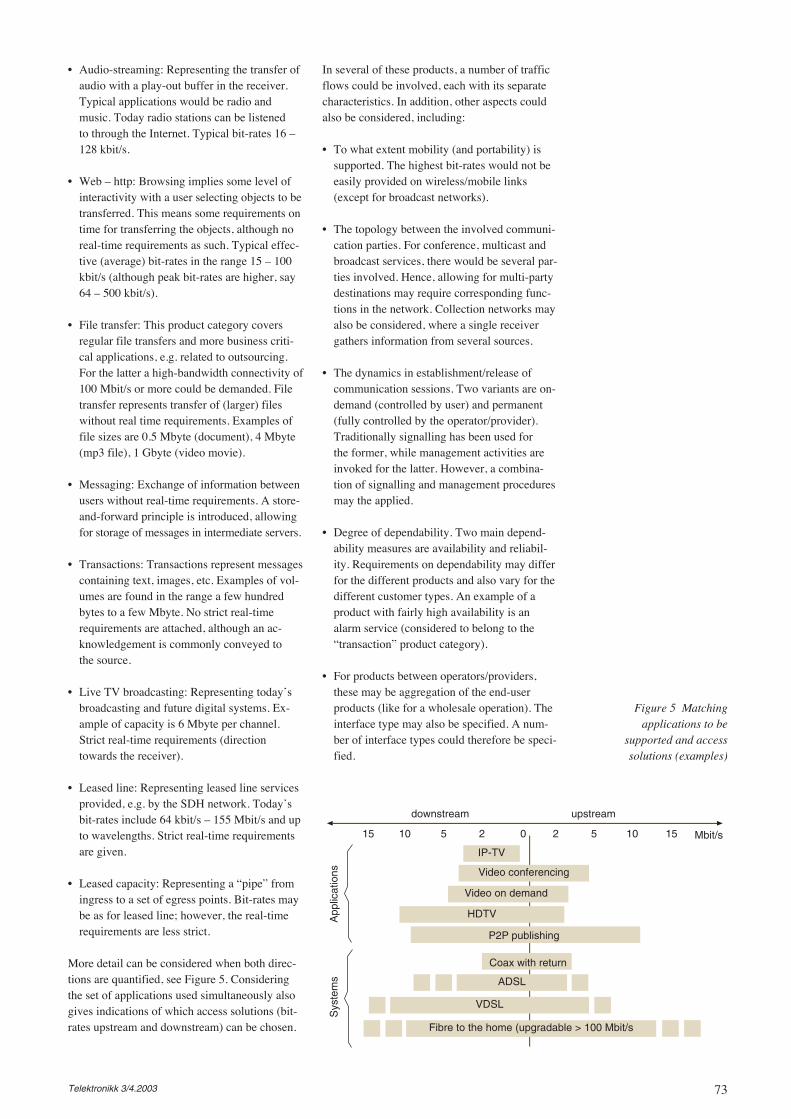
73Telektronikk 3/4.2003
• Audio-streaming: Representing the transfer ofaudio with a play-out buffer in the receiver.Typical applications would be radio andmusic. Today radio stations can be listenedto through the Internet. Typical bit-rates 16 –128 kbit/s.
• Web – http: Browsing implies some level ofinteractivity with a user selecting objects to betransferred. This means some requirements ontime for transferring the objects, although noreal-time requirements as such. Typical effec-tive (average) bit-rates in the range 15 – 100kbit/s (although peak bit-rates are higher, say64 – 500 kbit/s).
• File transfer: This product category coversregular file transfers and more business criti-cal applications, e.g. related to outsourcing.For the latter a high-bandwidth connectivity of100 Mbit/s or more could be demanded. Filetransfer represents transfer of (larger) fileswithout real time requirements. Examples offile sizes are 0.5 Mbyte (document), 4 Mbyte(mp3 file), 1 Gbyte (video movie).
• Messaging: Exchange of information betweenusers without real-time requirements. A store-and-forward principle is introduced, allowingfor storage of messages in intermediate servers.
• Transactions: Transactions represent messagescontaining text, images, etc. Examples of vol-umes are found in the range a few hundredbytes to a few Mbyte. No strict real-timerequirements are attached, although an ac-knowledgement is commonly conveyed tothe source.
• Live TV broadcasting: Representing today’sbroadcasting and future digital systems. Ex-ample of capacity is 6 Mbyte per channel.Strict real-time requirements (directiontowards the receiver).
• Leased line: Representing leased line servicesprovided, e.g. by the SDH network. Today’sbit-rates include 64 kbit/s – 155 Mbit/s and upto wavelengths. Strict real-time requirementsare given.
• Leased capacity: Representing a “pipe” fromingress to a set of egress points. Bit-rates maybe as for leased line; however, the real-timerequirements are less strict.
More detail can be considered when both direc-tions are quantified, see Figure 5. Consideringthe set of applications used simultaneously alsogives indications of which access solutions (bit-rates upstream and downstream) can be chosen.
In several of these products, a number of trafficflows could be involved, each with its separatecharacteristics. In addition, other aspects couldalso be considered, including:
• To what extent mobility (and portability) issupported. The highest bit-rates would not beeasily provided on wireless/mobile links(except for broadcast networks).
• The topology between the involved communi-cation parties. For conference, multicast andbroadcast services, there would be several par-ties involved. Hence, allowing for multi-partydestinations may require corresponding func-tions in the network. Collection networks mayalso be considered, where a single receivergathers information from several sources.
• The dynamics in establishment/release ofcommunication sessions. Two variants are on-demand (controlled by user) and permanent(fully controlled by the operator/provider).Traditionally signalling has been used forthe former, while management activities areinvoked for the latter. However, a combina-tion of signalling and management proceduresmay the applied.
• Degree of dependability. Two main depend-ability measures are availability and reliabil-ity. Requirements on dependability may differfor the different products and also vary for thedifferent customer types. An example of aproduct with fairly high availability is analarm service (considered to belong to the“transaction” product category).
• For products between operators/providers,these may be aggregation of the end-userproducts (like for a wholesale operation). Theinterface type may also be specified. A num-ber of interface types could therefore be speci-fied.
Figure 5 Matchingapplications to be
supported and accesssolutions (examples)
10 5 2 0
Fibre to the home (upgradable > 100 Mbit/s
15 2 5 10 15
downstream upstream
Mbit/s
IP-TV
Video on demand
Video conferencing
HDTV
P2P publishing
Coax with return
ADSL
VDSL
App
licat
ions
Sys
tem
s
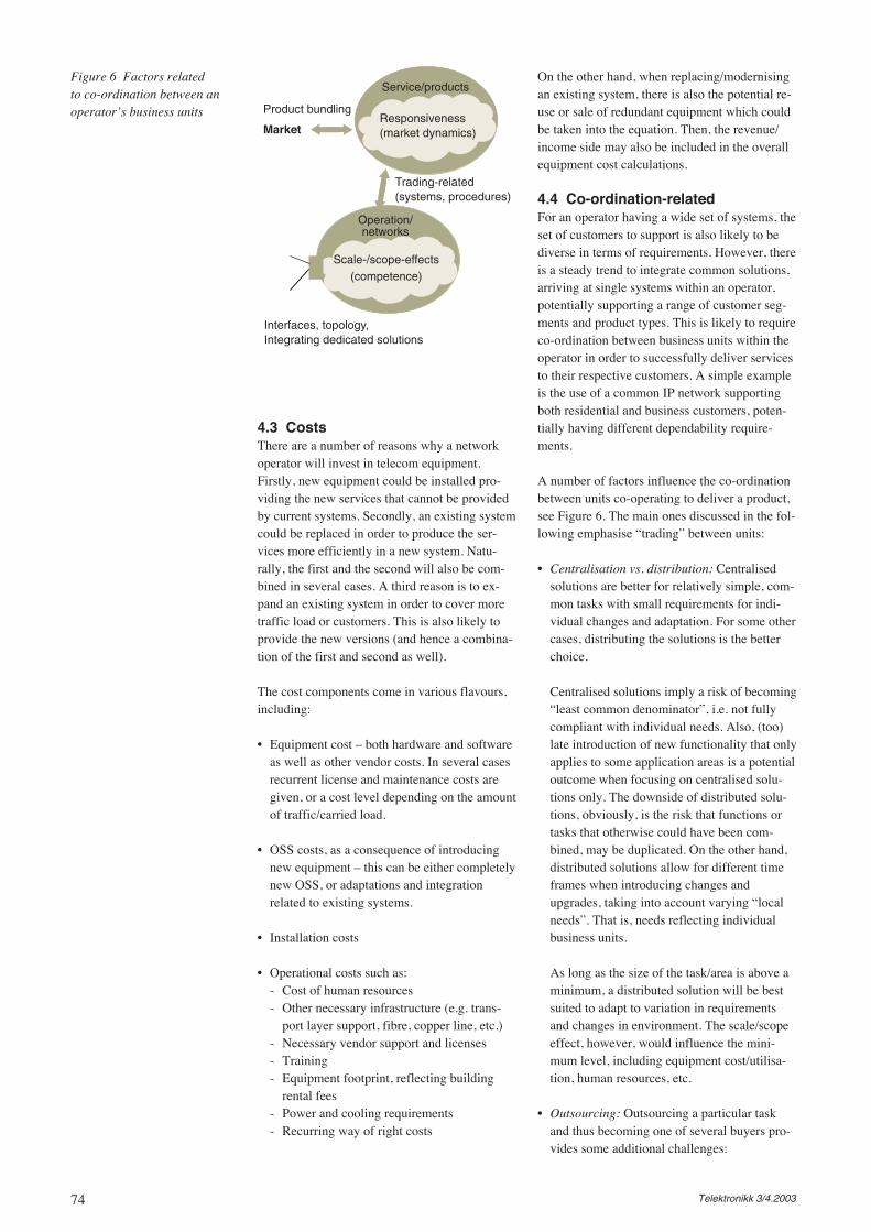
74 Telektronikk 3/4.2003
4.3 CostsThere are a number of reasons why a networkoperator will invest in telecom equipment.Firstly, new equipment could be installed pro-viding the new services that cannot be providedby current systems. Secondly, an existing systemcould be replaced in order to produce the ser-vices more efficiently in a new system. Natu-rally, the first and the second will also be com-bined in several cases. A third reason is to ex-pand an existing system in order to cover moretraffic load or customers. This is also likely toprovide the new versions (and hence a combina-tion of the first and second as well).
The cost components come in various flavours,including:
• Equipment cost – both hardware and softwareas well as other vendor costs. In several casesrecurrent license and maintenance costs aregiven, or a cost level depending on the amountof traffic/carried load.
• OSS costs, as a consequence of introducingnew equipment – this can be either completelynew OSS, or adaptations and integrationrelated to existing systems.
• Installation costs
• Operational costs such as:- Cost of human resources- Other necessary infrastructure (e.g. trans-
port layer support, fibre, copper line, etc.)- Necessary vendor support and licenses- Training- Equipment footprint, reflecting building
rental fees- Power and cooling requirements- Recurring way of right costs
On the other hand, when replacing/modernisingan existing system, there is also the potential re-use or sale of redundant equipment which couldbe taken into the equation. Then, the revenue/income side may also be included in the overallequipment cost calculations.
4.4 Co-ordination-relatedFor an operator having a wide set of systems, theset of customers to support is also likely to bediverse in terms of requirements. However, thereis a steady trend to integrate common solutions,arriving at single systems within an operator,potentially supporting a range of customer seg-ments and product types. This is likely to requireco-ordination between business units within theoperator in order to successfully deliver servicesto their respective customers. A simple exampleis the use of a common IP network supportingboth residential and business customers, poten-tially having different dependability require-ments.
A number of factors influence the co-ordinationbetween units co-operating to deliver a product,see Figure 6. The main ones discussed in the fol-lowing emphasise “trading” between units:
• Centralisation vs. distribution: Centralisedsolutions are better for relatively simple, com-mon tasks with small requirements for indi-vidual changes and adaptation. For some othercases, distributing the solutions is the betterchoice.
Centralised solutions imply a risk of becoming“least common denominator”, i.e. not fullycompliant with individual needs. Also, (too)late introduction of new functionality that onlyapplies to some application areas is a potentialoutcome when focusing on centralised solu-tions only. The downside of distributed solu-tions, obviously, is the risk that functions ortasks that otherwise could have been com-bined, may be duplicated. On the other hand,distributed solutions allow for different timeframes when introducing changes andupgrades, taking into account varying “localneeds”. That is, needs reflecting individualbusiness units.
As long as the size of the task/area is above aminimum, a distributed solution will be bestsuited to adapt to variation in requirementsand changes in environment. The scale/scopeeffect, however, would influence the mini-mum level, including equipment cost/utilisa-tion, human resources, etc.
• Outsourcing: Outsourcing a particular taskand thus becoming one of several buyers pro-vides some additional challenges:
Figure 6 Factors relatedto co-ordination between anoperator’s business units
Market
Product bundling
Trading-related(systems, procedures)
Scale-/scope-effects(competence)
Interfaces, topology,Integrating dedicated solutions
Service/products
Responsiveness(market dynamics)
Operation/networks
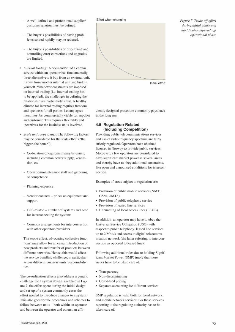
75Telektronikk 3/4.2003
- A well-defined and professional supplier/customer relation must be defined.
- The buyer’s possibilities of having prob-lems solved rapidly may be reduced.
- The buyer’s possibilities of prioritising andcontrolling error corrections and upgradesare limited.
• Internal trading: A “demander” of a certainservice within an operator has fundamentallythree alternatives: i) buy from an external unit,ii) buy from another internal unit, iii) build ityourself. Whenever constraints are imposedon internal trading (i.e. internal trading hasto be applied), the challenges in defining therelationship are particularly great. A healthyclimate for internal trading requires freedomand openness for all parties, i.e. any agree-ment must be commercially viable for supplierand customer. This requires flexibility andincentives for the business units involved.
• Scale and scope issues: The following factorsmay be considered for the scale effect (“thebigger, the better”):
- Co-location of equipment may be easier,including common power supply, ventila-tion, etc.
- Operation/maintenance staff and gatheringof competence
- Planning expertise
- Vendor contacts – prices on equipment andsupport
- OSS-related – number of systems and needfor interconnecting the systems
- Common arrangements for interconnectionwith other operators/providers
The scope effect, advocating collective func-tions, may allow for an easier introduction ofnew products and transfer of products betweendifferent networks. Hence, this would affectthe service bundling challenge, in particularacross different business units’ responsibili-ties.
The co-ordination effects also address a genericchallenge for a system design, sketched in Fig-ure 7; the effort spent during the initial designand set-up of a system commonly eases theeffort needed to introduce changes to a system.This also goes for the procedures and schemes tofollow between units – both within an operatorand between the operator and others; an effi-
ciently designed procedure commonly pays backin the long run.
4.5 Regulation-Related (Including Competition)
Providing public telecommunications servicesand use of radio frequency spectrum are fairlystrictly regulated. Operators have obtainedlicenses in Norway to provide public services.Moreover, a few operators are considered tohave significant market power in several areasand thereby have to obey additional constraints,like open and announced conditions for intercon-nection.
Examples of areas subject to regulation are:
• Provision of public mobile services (NMT,GSM, UMTS)
• Provision of public telephony service• Provision of leased line services• Unbundling of local access lines (LLUB)
In addition, an operator may have to obey theUniversal Service Obligation (USO) withrespect to public telephony, leased line servicesup to 2 Mbit/s and access to digital telecommu-nication network (the latter referring to intercon-nection as opposed to leased line).
Following additional rules due to holding Signif-icant Market Power (SMP) imply that moreissues have to be taken care of:
• Transparency• Non-discriminating• Cost-based pricing• Separate accounting for different services
SMP regulation is valid both for fixed networkand mobile network services. For these servicesreporting to the regulating authority has to betaken care of.
Figure 7 Trade-off effortduring initial phase andmodification/upgrading/
operational phase
Effort when changing
Initial effort
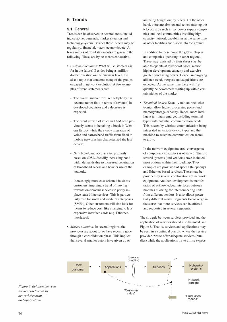
76 Telektronikk 3/4.2003
5 Trends
5.1 GeneralTrends can be observed in several areas, includ-ing customer demands, market situation andtechnology/system. Besides these, others may beregulatory, financial, macro-economic, etc. Afew samples of trend statements are given in thefollowing. These are by no means exhaustive.
• Customer demands: What will customers askfor in the future? Besides being a “million-dollar” question on the business level, it isalso a topic that concerns many of the groupsengaged in network evolution. A few exam-ples of trend statements are:
- The overall market for fixed telephony hasbecome rather flat (in terms of revenue) indeveloped countries and a decrease isexpected.
- The rapid growth of voice in GSM seen pre-viously seems to be taking a break in West-ern Europe while the steady migration ofvoice and narrowband traffic from fixed tomobile networks has characterized the lastdecade.
- New broadband accesses are primarilybased on xDSL. Steadily increasing band-width demands due to increased penetrationof broadband access and heavier use of thenetwork.
- Increasingly more cost-oriented businesscustomers, implying a trend of movingtowards on-demand services to partly re-place leased-line services. This is particu-larly true for small and medium enterprises(SMEs). Other customers will also look formeans to reduce cost, like changing to lessexpensive interface cards (e.g. Ethernet-interfaces).
• Market situation: In several regions, theproviders are about to, or have recently gonethrough a consolidation phase. This impliesthat several smaller actors have given up or
are being bought out by others. On the otherhand, there are also several actors entering thetelecom area such as the power supply compa-nies and local communities installing highcapacity network capabilities at the same timeas other facilities are placed into the ground.
In addition to these come the global playersand companies operating in other regions.These may, assisted by their sheer size, beable to operate at lower cost bases, realisehigher development capacity and exercisegreater purchasing power. Hence, an on-goingalliance trend, mergers and acquisitions areexpected. At the same time there will fre-quently be newcomers starting up within cer-tain niches of the market.
• Technical issues: Steadily miniaturized elec-tronics allow higher processing power andmemory/storage capacity. Hence, more intel-ligent terminals emerge, including terminaltypes with potential communication needs.This is seen by wireless communication beingintegrated in various device types and thatmachine-to-machine communication seemsto grow.
In the network equipment area, convergenceof equipment capabilities is observed. That is,several systems (and vendors) have includedmost options within their roadmap. Twoexamples are provision of speech (telephony)and Ethernet-based services. These may beprovided by several combinations of networkequipment. Another development is manifes-tation of acknowledged interfaces betweenmodules allowing for interconnecting unitsfrom different vendors. It also allows poten-tially different market segments to converge inthe sense that more services can be offeredand requested in several segments.
The struggle between services provided and theapplication of services should also be noted, seeFigure 8. That is, services and applications maybe seen in a continual pursuit; where the serviceprovider tries to offer adequate services (bun-dles) while the applications try to utilise expect-
Figure 8 Relation betweenservices (delivered bynetworks/systems) and applications
User/
customerApplications Services Networks/
systems
Servicebundling
Networkportions
”Productionmeans”
”Customervalue”
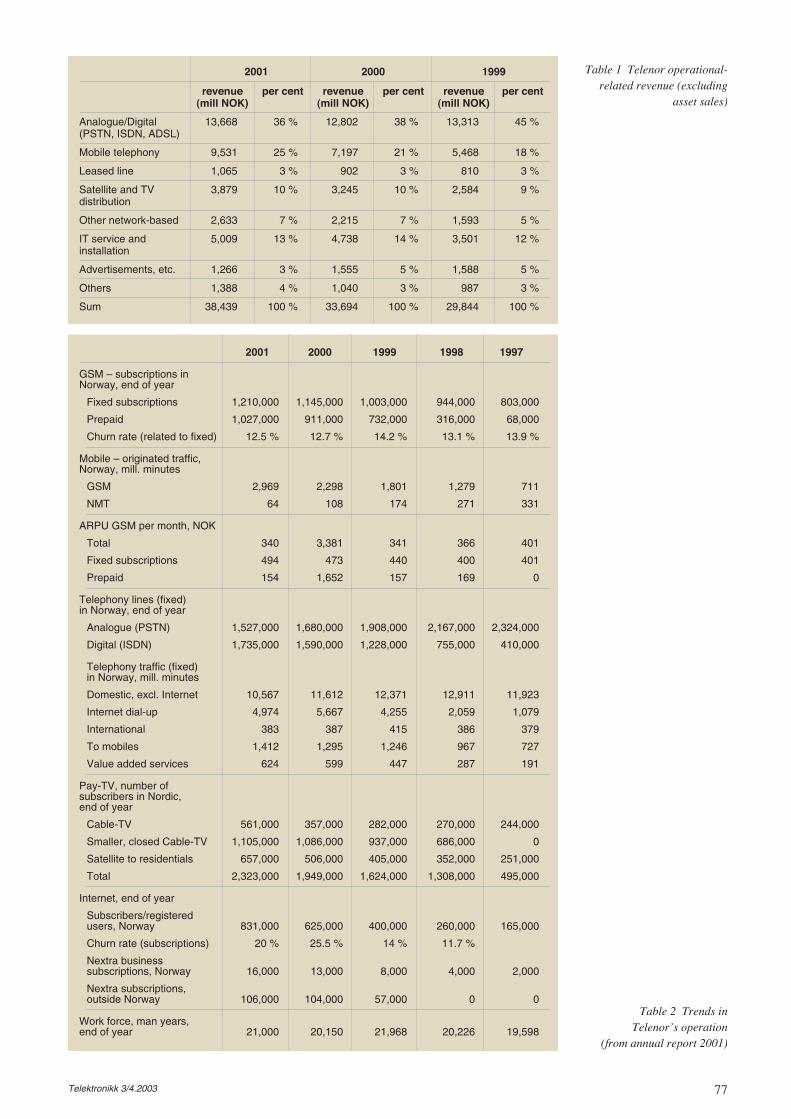
77Telektronikk 3/4.2003
2001 2000 1999
revenue per cent revenue per cent revenue per cent(mill NOK) (mill NOK) (mill NOK)
Analogue/Digital 13,668 36 % 12,802 38 % 13,313 45 %(PSTN, ISDN, ADSL)
Mobile telephony 9,531 25 % 7,197 21 % 5,468 18 %
Leased line 1,065 3 % 902 3 % 810 3 %
Satellite and TV 3,879 10 % 3,245 10 % 2,584 9 %distribution
Other network-based 2,633 7 % 2,215 7 % 1,593 5 %
IT service and 5,009 13 % 4,738 14 % 3,501 12 %installation
Advertisements, etc. 1,266 3 % 1,555 5 % 1,588 5 %
Others 1,388 4 % 1,040 3 % 987 3 %
Sum 38,439 100 % 33,694 100 % 29,844 100 %
Table 1 Telenor operational-related revenue (excluding
asset sales)
2001 2000 1999 1998 1997
GSM – subscriptions in Norway, end of year
Fixed subscriptions 1,210,000 1,145,000 1,003,000 944,000 803,000
Prepaid 1,027,000 911,000 732,000 316,000 68,000
Churn rate (related to fixed) 12.5 % 12.7 % 14.2 % 13.1 % 13.9 %
Mobile – originated traffic, Norway, mill. minutes
GSM 2,969 2,298 1,801 1,279 711
NMT 64 108 174 271 331
ARPU GSM per month, NOK
Total 340 3,381 341 366 401
Fixed subscriptions 494 473 440 400 401
Prepaid 154 1,652 157 169 0
Telephony lines (fixed) in Norway, end of year
Analogue (PSTN) 1,527,000 1,680,000 1,908,000 2,167,000 2,324,000
Digital (ISDN) 1,735,000 1,590,000 1,228,000 755,000 410,000
Telephony traffic (fixed) in Norway, mill. minutes
Domestic, excl. Internet 10,567 11,612 12,371 12,911 11,923
Internet dial-up 4,974 5,667 4,255 2,059 1,079
International 383 387 415 386 379
To mobiles 1,412 1,295 1,246 967 727
Value added services 624 599 447 287 191
Pay-TV, number of subscribers in Nordic, end of year
Cable-TV 561,000 357,000 282,000 270,000 244,000
Smaller, closed Cable-TV 1,105,000 1,086,000 937,000 686,000 0
Satellite to residentials 657,000 506,000 405,000 352,000 251,000
Total 2,323,000 1,949,000 1,624,000 1,308,000 495,000
Internet, end of year
Subscribers/registeredusers, Norway 831,000 625,000 400,000 260,000 165,000
Churn rate (subscriptions) 20 % 25.5 % 14 % 11.7 %
Nextra business subscriptions, Norway 16,000 13,000 8,000 4,000 2,000
Nextra subscriptions, outside Norway 106,000 104,000 57,000 0 0
Work force, man years, end of year 21,000 20,150 21,968 20,226 19,598
Table 2 Trends inTelenor’s operation
(from annual report 2001)
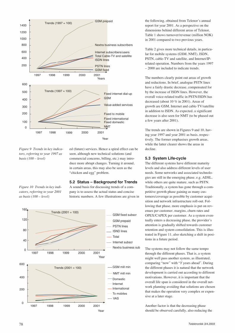
78 Telektronikk 3/4.2003
ed (future) services. Hence a spiral effect can beseen, although new technical solutions (andcommercial concerns, billing, etc.) may intro-duce more abrupt changes. Turning it around,in certain areas, this may also be seen as the“chicken and egg” problem.
5.2 Status – Background for TrendsA sound basis for discussing trends of a com-pany is to assess the actual status and concisehistoric numbers. A few illustrations are given in
the following, obtained from Telenor’s annualreport for year 2001. As a perspective on thedimensions behind different areas of Telenor,Table 1 shows turnover/revenue (million NOK)in 2001 compared to two previous years.
Table 2 gives more technical details, in particu-lar for mobile systems (GSM, NMT), ISDN,PSTN, cable-TV and satellite, and Internet/IP-related operation. Numbers from the years 1997– 2000 are included to indicate trends.
The numbers clearly point out areas of growthand reductions. In brief, analogue PSTN lineshave a fairly drastic decrease, compensated forby the increase of ISDN lines. However, theoverall voice-related traffic in PSTN/ISDN hasdecreased (about 10 % in 2001). Areas ofgrowth are GSM, Internet and cable-TV/satellitein addition to ISDN. As expected, a significantdecrease is also seen for NMT (to be phased outa few years after 2001).
The trends are shown in Figures 9 and 10, hav-ing year 1997 and year 2001 as basis, respec-tively. The former emphasises growth areas,while the latter clearer shows the areas indecline.
5.3 System Life-cycleThe different systems have different maturitylevels and also address different levels of userneeds. Some networks and associated technolo-gies are still in the emerging phase, e.g. ADSL,while others are quite mature, such as PSTN.Traditionally, a system has gone through a com-petitive growth phase gaining as many cus-tomers/coverage as possible by customer acqui-sition and network infrastructure roll-out. Fol-lowing that phase, more emphasis is put on rev-enues per customer, margins, churn rates andOPEX/CAPEX per customer. As a system even-tually enters a decreasing phase, the provider’sattention is gradually shifted towards customerretention and system consolidation. This is illus-trated in Figure 11, also sketching a shift in posi-tions in a future period.
The systems may not follow the same tempothrough the different phases. That is, a systemmight well pass another system, as illustrated,comparing “now” with “Y years ahead”. Duringthe different phases it is natural that the networkdevelopment is carried out according to differentmotivations. However, it is important that theoverall life span is considered in the overall net-work planning avoiding that solutions are chosenthat makes the operation very complex or expen-sive at a later stage.
Another factor is that the decreasing phaseshould be observed carefully, also reducing the
Figure 9 Trends in key indica-tors, referring to year 1997 asbasis (100 – level)
Figure 10 Trends in key indi-cators, referring to year 2001as basis (100 – level)
Trends (1997 = 100)
200
400
600
800
1000
1200
1400
1997 1998 1999 2000 2001Years
GSM prepaid
Nextra business subscribers
Internet subscribers/usersTotal Cable-TV and satelliteISDN lines
GSM fixedPSTN lines
Trends (1997 = 100)
0
100
200
300
400
500
600
1997 1998 1999 2000 2001
Year
Fixed internet dial-up
GSM
Value-added services
Fixed to mobile
Fixed domestic
NMT
Fixed international
Trends (2001 = 100)
0
40
80
120
160
1997 1998 1999 2000 2001Year
Total
PSTN lines
GSM fixed subscr
ISND lines
Internet subscr
Nextra business sub
GSM prepaid
0
200
400
600
1997 1998 1999 2000 2001
Year
Trends (2001 = 100) GSM mill min
NMT mill min
Domestic
Internet
International
To mobiles
VAS
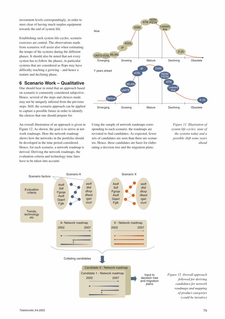
79Telektronikk 3/4.2003
investment levels correspondingly, in order tosteer clear of having much surplus equipmenttowards the end of system life.
Establishing such system life-cycles, scenarioexercises are central. The observations madefrom scenarios will assist also when estimatingthe tempo of the systems during the differentphases. It should also be noted that not everysystem has to follow the phases, in particularsystems that are considered as flops may havedifficulty reaching a growing – and hence amature and declining phase.
6 Scenario Work – QualitativeOne should bear in mind that an approach basedon scenario is commonly considered subjective.Hence, several of the steps and choices mademay not be uniquely inferred from the previoussteps. Still, the scenario approach can be appliedto capture a possible future in order to identifythe choices that one should prepare for.
An overall illustration of an approach is given inFigure 12. As shown, the goal is to arrive at net-work roadmaps. Here the network roadmapshows how the networks in the portfolio shouldbe developed in the time period considered.Hence, for each scenario, a network roadmap isderived. Deriving the network roadmaps, theevaluation criteria and technology time lineshave to be taken into account.
Using the sample of network roadmaps corre-sponding to each scenario, the roadmaps arerevisited to find candidates. As expected, fewersets of candidates are seen than there are scenar-ios. Hence, these candidates are basis for elabo-rating a decision tree and the migration plans.
Figure 11 Illustration ofsystem life-cycles; state of
the systems today and apossible shift some years
ahead
Mature Obsolete
Leasedline
Emerging Growing Declining
ISDN/PSTNATM
X.25
GSM
IP
ADSL
VDSLUMTS
Now
Y years ahead
WLAN
Optical
Leasedline
ISDN/PSTN
ATM
GSM
UMTS
WLAN
xDSL
IP
X.25
Mature ObsoleteEmerging Growing Declining
Scenario factors
Evaluationcriteria
Trends,technology
etc
Scenario A
AsdfSdf
FgoqeAsdfGqertFglk
asdfdfaf
dfoqrdfasdigwtoiurt
AsdfSdf
FgoqeAsdfGqertFglk
asdfdfaf
dfoqrdfasdigwtoiurt
Scenario X
X - Network roadmap
2002 2007
A- Network roadmap
2002 2007
Candidate 1 - Network roadmap
2002 2007
Candidate X - Network roadmap
Collating candidates
Input todecision treeand migration
plans
Figure 12 Overall approachfollowed for deriving
candidates for networkroadmaps and mapping
of product categories (could be iterative)
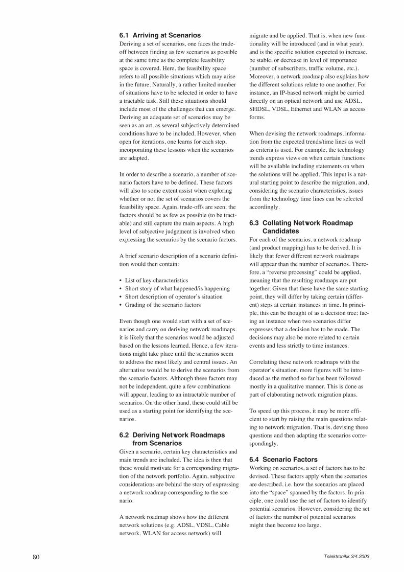
80 Telektronikk 3/4.2003
6.1 Arriving at ScenariosDeriving a set of scenarios, one faces the trade-off between finding as few scenarios as possibleat the same time as the complete feasibilityspace is covered. Here, the feasibility spacerefers to all possible situations which may arisein the future. Naturally, a rather limited numberof situations have to be selected in order to havea tractable task. Still these situations shouldinclude most of the challenges that can emerge.Deriving an adequate set of scenarios may beseen as an art, as several subjectively determinedconditions have to be included. However, whenopen for iterations, one learns for each step,incorporating these lessons when the scenariosare adapted.
In order to describe a scenario, a number of sce-nario factors have to be defined. These factorswill also to some extent assist when exploringwhether or not the set of scenarios covers thefeasibility space. Again, trade-offs are seen; thefactors should be as few as possible (to be tract-able) and still capture the main aspects. A highlevel of subjective judgement is involved whenexpressing the scenarios by the scenario factors.
A brief scenario description of a scenario defini-tion would then contain:
• List of key characteristics• Short story of what happened/is happening• Short description of operator’s situation• Grading of the scenario factors
Even though one would start with a set of sce-narios and carry on deriving network roadmaps,it is likely that the scenarios would be adjustedbased on the lessons learned. Hence, a few itera-tions might take place until the scenarios seemto address the most likely and central issues. Analternative would be to derive the scenarios fromthe scenario factors. Although these factors maynot be independent, quite a few combinationswill appear, leading to an intractable number ofscenarios. On the other hand, these could still beused as a starting point for identifying the sce-narios.
6.2 Deriving Network Roadmapsfrom Scenarios
Given a scenario, certain key characteristics andmain trends are included. The idea is then thatthese would motivate for a corresponding migra-tion of the network portfolio. Again, subjectiveconsiderations are behind the story of expressinga network roadmap corresponding to the sce-nario.
A network roadmap shows how the differentnetwork solutions (e.g. ADSL, VDSL, Cablenetwork, WLAN for access network) will
migrate and be applied. That is, when new func-tionality will be introduced (and in what year),and is the specific solution expected to increase,be stable, or decrease in level of importance(number of subscribers, traffic volume, etc.).Moreover, a network roadmap also explains howthe different solutions relate to one another. Forinstance, an IP-based network might be carrieddirectly on an optical network and use ADSL,SHDSL, VDSL, Ethernet and WLAN as accessforms.
When devising the network roadmaps, informa-tion from the expected trends/time lines as wellas criteria is used. For example, the technologytrends express views on when certain functionswill be available including statements on whenthe solutions will be applied. This input is a nat-ural starting point to describe the migration, and,considering the scenario characteristics, issuesfrom the technology time lines can be selectedaccordingly.
6.3 Collating Network RoadmapCandidates
For each of the scenarios, a network roadmap(and product mapping) has to be derived. It islikely that fewer different network roadmapswill appear than the number of scenarios. There-fore, a “reverse processing” could be applied,meaning that the resulting roadmaps are puttogether. Given that these have the same startingpoint, they will differ by taking certain (differ-ent) steps at certain instances in time. In princi-ple, this can be thought of as a decision tree; fac-ing an instance when two scenarios differexpresses that a decision has to be made. Thedecisions may also be more related to certainevents and less strictly to time instances.
Correlating these network roadmaps with theoperator’s situation, more figures will be intro-duced as the method so far has been followedmostly in a qualitative manner. This is done aspart of elaborating network migration plans.
To speed up this process, it may be more effi-cient to start by raising the main questions relat-ing to network migration. That is, devising thesequestions and then adapting the scenarios corre-spondingly.
6.4 Scenario FactorsWorking on scenarios, a set of factors has to bedevised. These factors apply when the scenariosare described, i.e. how the scenarios are placedinto the “space” spanned by the factors. In prin-ciple, one could use the set of factors to identifypotential scenarios. However, considering the setof factors the number of potential scenariosmight then become too large.
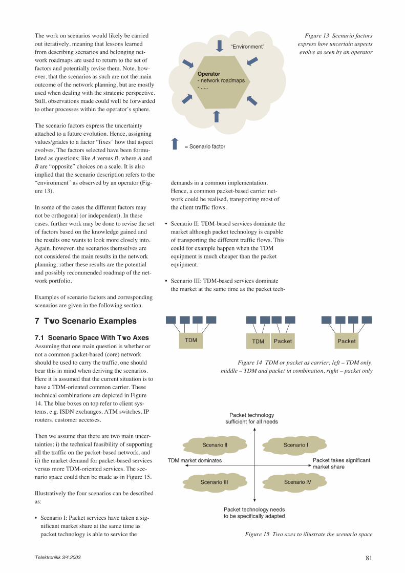
81Telektronikk 3/4.2003
The work on scenarios would likely be carriedout iteratively, meaning that lessons learnedfrom describing scenarios and belonging net-work roadmaps are used to return to the set offactors and potentially revise them. Note, how-ever, that the scenarios as such are not the mainoutcome of the network planning, but are mostlyused when dealing with the strategic perspective.Still, observations made could well be forwardedto other processes within the operator’s sphere.
The scenario factors express the uncertaintyattached to a future evolution. Hence, assigningvalues/grades to a factor “fixes” how that aspectevolves. The factors selected have been formu-lated as questions; like A versus B, where A andB are “opposite” choices on a scale. It is alsoimplied that the scenario description refers to the“environment” as observed by an operator (Fig-ure 13).
In some of the cases the different factors maynot be orthogonal (or independent). In thesecases, further work may be done to revise the setof factors based on the knowledge gained andthe results one wants to look more closely into.Again, however, the scenarios themselves arenot considered the main results in the networkplanning; rather these results are the potentialand possibly recommended roadmap of the net-work portfolio.
Examples of scenario factors and correspondingscenarios are given in the following section.
7 Two Scenario Examples
7.1 Scenario Space With Two AxesAssuming that one main question is whether ornot a common packet-based (core) networkshould be used to carry the traffic, one shouldbear this in mind when deriving the scenarios.Here it is assumed that the current situation is tohave a TDM-oriented common carrier. Thesetechnical combinations are depicted in Figure14. The blue boxes on top refer to client sys-tems, e.g. ISDN exchanges, ATM switches, IProuters, customer accesses.
Then we assume that there are two main uncer-tainties; i) the technical feasibility of supportingall the traffic on the packet-based network, andii) the market demand for packet-based servicesversus more TDM-oriented services. The sce-nario space could then be made as in Figure 15.
Illustratively the four scenarios can be describedas:
• Scenario I: Packet services have taken a sig-nificant market share at the same time aspacket technology is able to service the
demands in a common implementation.Hence, a common packet-based carrier net-work could be realised, transporting most ofthe client traffic flows.
• Scenario II: TDM-based services dominate themarket although packet technology is capableof transporting the different traffic flows. Thiscould for example happen when the TDMequipment is much cheaper than the packetequipment.
• Scenario III: TDM-based services dominatethe market at the same time as the packet tech-
Figure 15 Two axes to illustrate the scenario space
Figure 13 Scenario factorsexpress how uncertain aspectsevolve as seen by an operator
Figure 14 TDM or packet as carrier; left – TDM only, middle – TDM and packet in combination, right – packet only
Operator- network roadmaps- .....
“Environment”
= Scenario factor
TDM TDM Packet Packet
Packet technologysufficient for all needs
Packet technology needsto be specifically adapted
Packet takes significantmarket share
TDM market dominates
Scenario III
Scenario II
Scenario IV
Scenario I
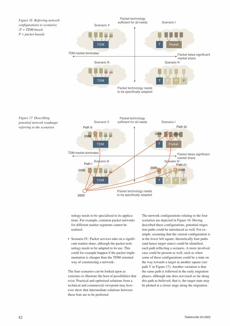
82 Telektronikk 3/4.2003
nology needs to be specialised to its applica-tions. For example, common packet networksfor different market segments cannot berealised.
• Scenario IV: Packet services take on a signifi-cant market share, although the packet tech-nology needs to be adapted to its use. Thiscould for example happen if the packet imple-mentation is cheaper than the TDM-orientedway of constructing a network.
The four scenarios can be looked upon asextremes to illustrate the host of possibilities thatexist. Practical and optimised solutions from atechnical and commercial viewpoint may how-ever show that intermediate solutions betweenthese four are to be preferred.
The network configurations relating to the fourscenarios are depicted in Figure 16. Havingdescribed these configurations, potential migra-tion paths could be introduced as well. For ex-ample, assuming that the current configuration isat the lower left square, theoretically four paths(and hence target states) could be identified,each path reflecting a scenario. A more involvedcase could be present as well, such as whensome of these configurations could be a state onthe way towards a target in another square (seepath V in Figure 17). Another variation is thatthe same path is followed in the early migrationphases, although one does not reach as far alongthis path as believed; that is, the target state maybe plotted at a closer stage along the migration.
Figure 16 Referring networkconfigurations to scenarios(T = TDM-based, P = packet-based)
Figure 17 Describingpotential network roadmapsreferring to the scenarios
Packet technologysufficient for all needs
Packet technology needsto be specifically adapted
Packet takes significantmarket share
TDM market dominates
PacketT
Scenario IIScenario I
TDM
Scenario III
TDM T
Scenario IV
P P P
Packet technologysufficient for all needs
Packet technology needsto be specifically adapted
Packet takes significantmarket share
TDM market dominates
PacketT
Scenario II Scenario I
TDM
Scenario III
TDM T
Scenario IV
P P P
Path II
Path IV
Path III
Path I
2003
20052008
200820082008
2008
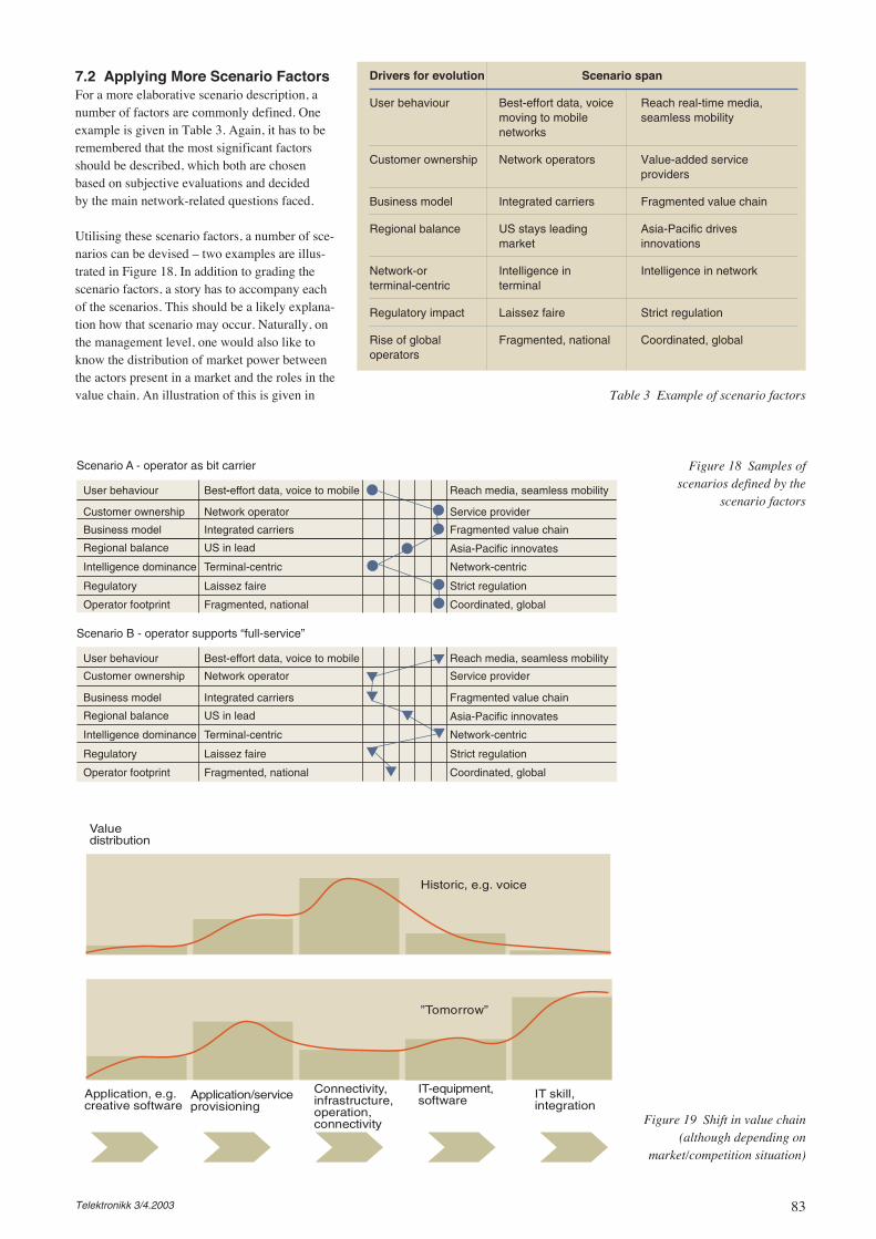
83Telektronikk 3/4.2003
7.2 Applying More Scenario FactorsFor a more elaborative scenario description, anumber of factors are commonly defined. Oneexample is given in Table 3. Again, it has to beremembered that the most significant factorsshould be described, which both are chosenbased on subjective evaluations and decidedby the main network-related questions faced.
Utilising these scenario factors, a number of sce-narios can be devised – two examples are illus-trated in Figure 18. In addition to grading thescenario factors, a story has to accompany eachof the scenarios. This should be a likely explana-tion how that scenario may occur. Naturally, onthe management level, one would also like toknow the distribution of market power betweenthe actors present in a market and the roles in thevalue chain. An illustration of this is given in
Drivers for evolution Scenario span
User behaviour Best-effort data, voice Reach real-time media, moving to mobile seamless mobilitynetworks
Customer ownership Network operators Value-added serviceproviders
Business model Integrated carriers Fragmented value chain
Regional balance US stays leading Asia-Pacific drivesmarket innovations
Network-or Intelligence in Intelligence in networkterminal-centric terminal
Regulatory impact Laissez faire Strict regulation
Rise of global Fragmented, national Coordinated, globaloperators
Table 3 Example of scenario factors
Figure 18 Samples ofscenarios defined by the
scenario factors
Figure 19 Shift in value chain(although depending on
market/competition situation)
Coordinated, globalFragmented, nationalOperator footprint
Strict regulationLaissez faireRegulatory
Network-centricTerminal-centricIntelligence dominance
Asia-Pacific innovatesUS in leadRegional balance
Fragmented value chainIntegrated carriersBusiness model
Service providerCustomer ownership
Reach media, seamless mobility-User behaviour
Network operator
Best-effort data, voice to mobile
Scenario A - operator as bit carrier
Scenario B - operator supports “full-service”
Coordinated, globalFragmented, nationalOperator footprint
Strict regulationLaissez faireRegulatory
Network-centricTerminal-centricIntelligence dominance
Asia-Pacific innovatesUS in leadRegional balance
Fragmented value chainIntegrated carriersBusiness model
Service providerCustomer ownership
Reach media, seamless mobilityUser behaviour
Network operator
Best-effort data, voice to mobile
Valuedistribution
Historic, e.g. voice
”Tomorrow”
Application, e.g.creative software
Application/serviceprovisioning
Connectivity,infrastructure,operation,connectivity
IT-equipment,software IT skill,
integration
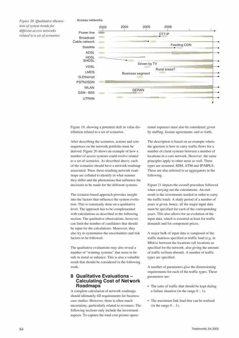
84 Telektronikk 3/4.2003
Figure 19, showing a potential shift in value dis-tribution related to a set of scenarios.
After describing the scenarios, actions and con-sequences on the network portfolio must bederived. Figure 20 shows an example of how anumber of access systems could evolve relatedto a set of scenarios. As described above, eachof the scenarios should have a network roadmapassociated. Then, these resulting network road-maps are collated to identify in what mannerthey differ and the phenomena that influence thedecisions to be made for the different systems.
The scenario-based approach provides insightinto the factors that influence the system evolu-tion. This is commonly done on a qualitativelevel. The approach has to be complementedwith calculations as described in the followingsection. The qualitative observations, however,can limit the number of candidates that shouldbe input for the calculations. Moreover, theyalso try to systematise the uncertainties and riskfactors to be followed.
The qualitative evaluations may also reveal anumber of “winning systems” that seem to besafe to instal or enhance. This is also a valuableresult that should be considered in the followingwork.
8 Qualitative Evaluations –Calculating Cost of NetworkRoadmaps
A complete calculation of network roadmapsshould ultimately fill requirements for businesscase studies. However, there is often muchuncertainty, particularly related to revenues. Thefollowing sections only include the investmentaspects. To capture the total cost picture opera-
tional expenses must also be considered, givenby staffing, license agreements, and so forth.
The description is based on an example wherethe question is how to carry traffic flows for anumber of client systems between a number oflocations in a core network. However, the sameprinciples apply to other areas as well. Threetypes are assumed, SDH, ATM and IP/MPLS.These are also referred to as aggregators in thefollowing.
Figure 21 depicts the overall procedure followedwhen carrying out the calculations. An end-result is the investments needed in order to carrythe traffic loads. A study period of a number ofyears is given, hence, all the major input datamust be specified for each of the correspondingyears. This also allows for an evolution of theinput data, which is essential at least for trafficdemands and for component prices.
A major bulk of input data is composed of thetraffic matrices specified as traffic load (e.g. inMbit/s) between the locations (all locations asspecified for the network, also giving the amountof traffic to/from abroad). A number of traffictypes are specified.
A number of parameters give the dimensioningrequirements for each of the traffic types. Theseparameters are:
• The ratio of traffic that should be kept duringa failure situation (in the range 0 .. 1),
• The maximum link load that can be realised(in the range 0 .. 1),
Figure 20 Qualitative illustra-tion of system trends fordifferent access networksrelated to a set of scenarios
2005 200620042003
Power line
BroadcastCable network
Satellite
Access networks
ADSL
SHDSL
VDSL
LMDS
G.Ethernet
PSTN/ISDN
WLAN
UTRAN
Feeding CDN
Rural areas?
Driven by TV
Business segment
GERAN
HDSL
GSM - BSS
DTT-IP
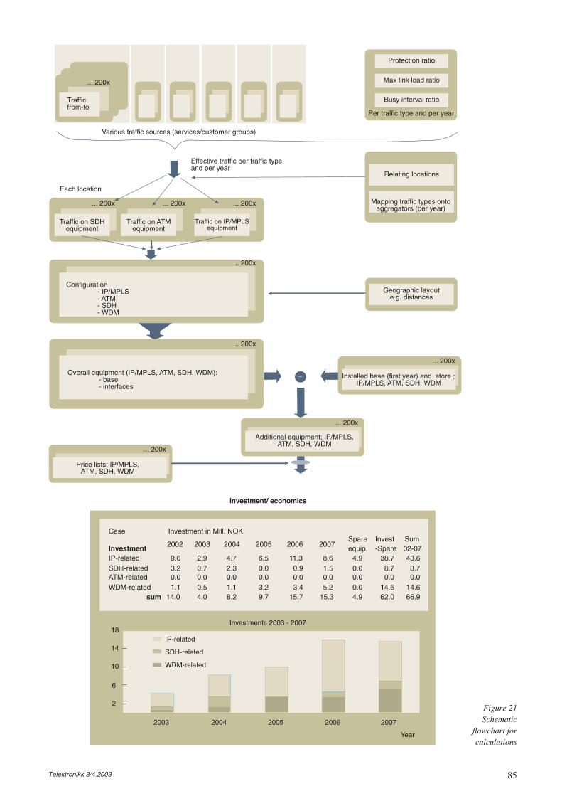
85Telektronikk 3/4.2003
... 200x
... 200x
Various traffic sources (services/customer groups)
Protection ratio
Max link load ratio
Per traffic type and per year
Relating locations
Busy interval ratio
Mapping traffic types ontoaggregators (per year)
Effective traffic per traffic typeand per year
Each location
... 200x ... 200x ... 200x
Traffic on SDHequipment
Traffic on ATMequipment
Traffic on IP/MPLSequipment
Configuration- IP/MPLS- ATM- SDH- WDM
... 200x
Geographic layoute.g. distances
Overall equipment (IP/MPLS, ATM, SDH, WDM):- base- interfaces
... 200x
... 200x
Additional equipment; IP/MPLS,ATM, SDH, WDM
Trafficfrom-to
Relating locations
Mapping traffic types ontoaggregators (per year)
Installed base (first year) and store ;IP/MPLS, ATM, SDH, WDM
... 200x
Price lists; IP/MPLS,ATM, SDH, WDM
Case Investment in Mill. NOK
2002 2003 2004 2005 2006 2007Spare Invest Sum
Investment equip. -Spare 02-07IP-related 9.6 2.9 4.7 6.5 11.3 8.6 4.9 38.7 43.6SDH-related 3.2 0.7 2.3 0.0 0.9 1.5 0.0 8.7 8.7ATM-related 0.0 0.0 0.0 0.0 0.0 0.0 0.0 0.0 0.0WDM-related 1.1 0.5 1.1 3.2 3.4 5.2 0.0 14.6 14.6
sum 14.0 4.0 8.2 9.7 15.7 15.3 4.9 62.0 66.9
Investments 2003 - 2007
2
6
10
14
18
2003 2004 2005 2006 2007
Year
IP-related
SDH-related
WDM-related
Investment/ economics
_
Figure 21 Schematic
flowchart forcalculations
86 Telektronikk 3/4.2003
• The relative portion of the peak traffic loadthat is present in the dimensioning interval,i.e. a busy interval indicator (in the range 0 ..1).
In combination, the two former indicate the traf-fic situation during a failure situation. For in-stance when a failure occurs, a ratio of the traffic(on the failed link) is carried by an alternativelink and the maximum load on that link is givenby the “maximum link load” parameter.
The result of taking these parameters intoaccount is called the effective traffic load. Thistraffic load is given for each traffic type andeach year. A step further is to consider the rela-tions between the locations. This means to con-sider where links are placed (present betweencertain locations). Relating the effective trafficloads, mapping of traffic types onto aggregatorsand presence of links decide the traffic load oneach aggregator type at each location.
The traffic loads on the aggregators give theconfigurations of each aggregator. “Directions”must also be included (that is where links aregoing) as well as the distances between the loca-tions (in particular for WDM equipment).
Adding equipment types on all locations givesthe overall needed equipment (for base configu-ration, interfaces, etc.). In order to consideractual deployment and equipment reuse betweendifferent years, an “equipment store” is present.Hence, only when needed equipment of a certaintype in a year exceeds the sum of that equipmenttype in the previous year and the number in the“store” is additional equipment bought.
The result after looking at installed equipment,“stored” equipment and needed equipment is alist of additional equipment that needs invest-ment funds. Considering the price of that equip-ment for the corresponding year gives an invest-ment level. These investments can be aggregatedin different ways, for instance per equipmentclass, per year, for the whole period, etc.
Figure 22 Costs of IP/MPLS, ATM, SDH and WDMequipment for cases and demand variations
Internet access pessimistic, L1LL baseline
0
20
40
60
80
100
Case A1 Case A2 Case B1 Case B2 Case C1 Case C2 Case D Case E
IP
ATM
SDH
WDM
Internet access optimistic, L1LL maximum
0
20
40
60
80
100
Case A1 Case A2 Case B1 Case B2 Case C1 Case C2 Case D Case E
IP
ATM
SDH
WDM
Internet access optimistic (50 % abroad), L1LL baseline
0
20
40
60
80
100
Case A1 Case A2 Case B1 Case B2 Case C1 Case C2 Case D Case E
IP
ATM
SDH
WDM
Internet access optimistic, L1LL baseline100
0
20
40
60
80
Case A1 Case A2 Case B1 Case B2 Case C1 Case C2 Case D Case E
WDM
IP
ATM
SDH
IP
ATM
SDH
WDM
Internet access optimistic, L1LL minimum
0
20
40
60
80
100
Case A1 Case A2 Case B1 Case B2 Case C1 Case C2 Case D Case E
87Telektronikk 3/4.2003
In addition to economic output, traffic andcapacity results can also be recorded.
Typically, calculations are carried out for a num-ber of cases and the results are compared. Thesecases can be specified by the technology used,years for introducing functionality, variation intraffic demands, changes in equipment prices,and so forth. In addition different network archi-tectures would be examined. An intention is tofind out the more critical parameters, that is,those significantly influencing the results and thenetwork roadmaps that should be preferred. Atthe end of the calculation period, the installedequipment could be assigned a value (“terminalvalue”) depending on how investment levelsshould be estimated.
For most transmission systems the capacity oftencomes in certain granularities, e.g. 155 Mbit/s,622 Mbit/s for SDH. This has to be included inaddition to any consequent costs such as man-agement systems and installation work.
An example of investment results is given inFigure 22. These are shown for five differentcombinations of traffic demands and where eightcases are examined (A1, .., E). One reason be-hind breaking up the investment cost showingnetwork types is to give ideas on where moreinvestment savings could be obtained.
An immediate observation from the resultsabove is the fairly high ratio of costs relating toIP/MPLS equipment. In order to look moreclosely into the effect of varying costs of thisequipment the following calculations were con-ducted; all IP/MPLS equipment costs werechanged by x % (in the interval from –75 % to+50 %). Only cases A1, A2 and D are shown inFigure 23 as the objective was to estimate pointsof intersections. Two demand variants areincluded: Internet access pessimistic + L1LL
baseline and Internet access optimistic + L1LLmaximum.
For the variant ‘Internet access optimistic +L1LL maximum’ cases A1 and D come out withequal overall investments when the IP/MPLScost is reduced by 25 %. For other combinationsthe IP/MPLS costs have to be reduced by about75 % in order for the lines to intersect.
9 Risk Analysis and ExitStrategies
As described earlier, a number of decisions willcommonly be revealed during the network strat-egy evaluations. For each step, a certain risklevel is associated. In this section a generalintroduction to incorporate risks into the evalua-tion given.
9.1 Risk – General IntroductionConsidering the constant change and uncer-tainty, an integrated risk management practicewithin an organisation is required to strategicallydeal with uncertainty and thereby capitalise onopportunities. The stakeholders in the decisionprocess will also be involved in order to ensurebetter decisions in the future.
A risk management arrangement should coverall types of risks that face the organisation,including policy, operational, human resources,financial, legal, health and safety, environment,reputation. Hence, it is essential to integrate riskmanagement into strategic decision-making. Byestablishing a risk management framework, amechanism will be in place allowing to discuss,compare and evaluate different risk types.
Deploying a risk management regime alsoallows for a so-called risk-smart workforce thatsupports innovative and responsible risk-takingwhile ensuring legitimate precautions.
Figure 23 Impact on IP/MPLScost variations for Cases A1,
A2 and D
IP/MPLS price variations
25 % 50 %
mill. NOK
Intern-pes; L1LL-base A1 sum
Intern-pes; L1LL-base A2 sum
Intern-pes; L1LL-base D sum
Intern-opt; L1LL-max A1 sum
Intern-opt; L1LL-max A2 sum
Intern-opt; L1LL-max D sum0
20
40
60
80
100
120
140
-75 % -50 % -25 % 0 %
88 Telektronikk 3/4.2003
Risk is unavoidable and present in almost everysituation in every-day life, for private as well asbusiness roles. A number of definitions of riskare in use. However, a common concept in alldefinitions is that a certain level of uncertaintyof the outcome is involved. One way the defini-tions differ is the characterisation of the out-comes; some describe risk as having onlyadverse consequences, while others are neutral.An ongoing discussion takes place arriving at anacceptable (common) generic definition of riskthat recognizes the fact that when assessed andmanaged properly, risk management can lead toinnovation and opportunity. This appears evenmore prevalent when dealing with operationalrisks and in the context of technological risks.One definition found is the expression of likeli-hood and impact of an event with the potentialto influence the achievement of an actor’s objec-tive. Hence, risk refers to uncertainty aroundfuture events and outcome.
Other definitions found are e.g.:
• Combination of the probability of an eventand its consequences. Note – in some situa-tions, risk is a deviation from the expected,
• The chance of something happening that willhave an impact on objectives. It is measuredin terms of consequences and likelihood,
• The chance of injury or loss defined as ameasure of the probability and severity of anadverse effect to health, property, the environ-ment or other things of value,
• The possibility that one or more individuals ororganizations will experience adverse conse-quences from an event or circumstance.
A risk measure can be formalised as
risk =
els as it concerns making decisions that con-tribute to the achievement of an actor’s objec-tives. Hence, integrated risk management is acontinuous, proactive and systematic process tounderstand, manage and communicate risk froman actor-wide perspective. It is about makingstrategic decisions that contribute to the achieve-ment of an actor’s overall corporate objectives.Integrated risk management requires an ongoingassessment of potential risks. Hence, it should beembedded in the actor’s strategy and risk man-agement culture. As stated above it is not limitedto minimising the risks, but rather to foster inno-vation in order to achieve greatest returns withacceptable results, costs and risks. Hence, anoptimal balance is strived for at the corporatelevel.
As pointed out in [Cari01], four key elementsare included in an integrated risk managementframework:
1. Develop the corporate risk profile – consider-ing objectives and available resourcesa. Identify risks; resulting in description of
threats and opportunities, i) type of risk –technological, financial, human resources,health, ii) source of risk – external, internal,iii) what is at risk – area of impact/type ofexposure, iv) level of ability to control therisk – high (operational), moderate (reputa-tion), low (natural disasters).
b. Assess current risk management status;resulting in descriptions of challenges/opportunities, capacity, practices.
c. Identify risk profile; description of key riskareas, risk tolerance, ability and capacity tomitigate and needs for learning. In general,there seems to be lower risk tolerance forthe unknown, where impacts are new, un-observable or delayed. In addition a higherrisk tolerance is observed where people feelmore in control (e.g. for car travel com-pared to air travel).
2. Establish an integrated risk management func-tiona. Communicate, understand and apply man-
agement direction on risk management; riskmanagement needs to be aligned with anactor’s overall objectives, corporate focus,strategic direction, operating practices andinternal culture. When a strategic risk man-agement direction is set up, both internaland external concerns, perceptions and risktolerances are taken into account. It isimperative to identify acceptable risk toler-ance levels so the unfavourable outcomescan be remedied promptly and effectively.
The summation is taken over all events consid-ered and the product of each event’s probabilityof occurring and consequence is added.
In order to take advantage of the present risk fac-tors a management framework should be intro-duced. Risk management is defined as a system-atic approach to setting the best course of actionunder uncertainty by identifying, assessing,understanding, acting on and communicatingrisk issues. As risk management is directed atuncertainty related to future events and out-comes, it is implied that all planning exercisesencompass some form of risk management. Riskmanagement is also impacting people at all lev-
∑
event i
probability(event i) · consequence(event i)
89Telektronikk 3/4.2003
b. Implement operational integrated risk man-agement through existing decision-makingand reporting structures. Integrating the riskmanagement function into existing strategicmanagement and operational processesensures that risk management is an integralpart of day-to-day activities.
c. Build capacity through development oflearning plans and tools. Building risk man-agement capacity is an ongoing challengeeven after integrated risk management hasbecome firmly entrenched. Environmentalscanning will continue to identify new areasand activities that require attention, as wellas the risk management skills, processes,and practices that need to be developed.
3. Practise integrated risk managementa. Consistent application of common risk
management at all levels. A common, con-tinuous risk management process assists anactor in understanding, managing and com-municating risk.
b. Integrate results of risk management prac-tices at all levels into informed decision-making and priority setting
c. Apply tools and methods
d. Consult and communicate with stakeholders
4. Ensure continuous risk management learninga. Establish supportive work environment
where learning from experience is valued,and lessons are shared
b. Build learning plans into actor’s risk man-agement practices
c. Evaluate results of risk management to sup-port innovation, learning and continuousimprovement
d. Share experiences and best practices
A potential risk management process wheel isillustrated in Figure 24. Internal and externalcommunication and continuous learning improveunderstanding and skills for risk managementpractice at all levels of an organisation, fromcorporate through to front-line operations. Thefollowing steps may be included in a risk man-agement process (from [Cari01]):
A. Risk Identification1. Identify issues, set context:
- Define the problems or opportunities,scope, context (social, cultural, scien-tific evidence, etc.) and associated riskissues.
- Decide on necessary people, expertise,tools and techniques (e.g. scenarios,brainstorming, checklists).
- Perform a stakeholder analysis (deter-mine risk tolerances, stakeholder posi-tion, attitudes).
B. Risk assessment2. Assess key risk areas:
- Analyse context/results of environmen-tal scan and define types/categories ofrisk to be addressed, significant organi-sation-wide issues, and vital localissues.
3. Measure likelihood and impact:- Determine degree of exposure, ex-
pressed as likelihood and impact, ofassessed risks, choose tools.
- Consider both the empirical/scientificevidence and public context.
4. Rank risks:- Rank risks, consider risk tolerance, use
existing or developing criteria and tools.
C. Respond to risk5. Set desired results:
- Define objectives and expected outcomefor ranked risks, short/long term.
6. Develope options:- Identify and analyse options – ways to
minimise threats and maximise opportu-nities – approaches, tools.
Practise integrated riskmanagement (from
corporate strategy andplans to front-line
operations – people andprocesses)
Continuous learningand communication
1: Identifyissues, settingcontext
2: Assessingkey riskareas
3: Measuringlikelihooodand impact
4: Rankingrisks
5: Settingdesiredresults
6:Developingoptions
7: Selectinga strategy
8: Imple-mentingthe strategy
9: Monitoring,evaluating andadjusting
Figure 24 A potential riskmanagement process
(adapted from [Cari01])
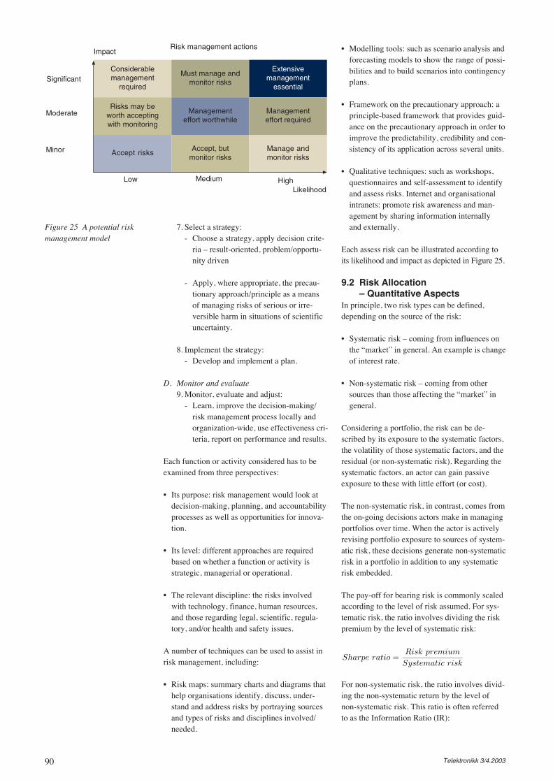
90 Telektronikk 3/4.2003
7. Select a strategy:- Choose a strategy, apply decision crite-
ria – result-oriented, problem/opportu-nity driven
- Apply, where appropriate, the precau-tionary approach/principle as a meansof managing risks of serious or irre-versible harm in situations of scientificuncertainty.
8. Implement the strategy:- Develop and implement a plan.
D. Monitor and evaluate9. Monitor, evaluate and adjust:
- Learn, improve the decision-making/risk management process locally andorganization-wide, use effectiveness cri-teria, report on performance and results.
Each function or activity considered has to beexamined from three perspectives:
• Its purpose: risk management would look atdecision-making, planning, and accountabilityprocesses as well as opportunities for innova-tion.
• Its level: different approaches are requiredbased on whether a function or activity isstrategic, managerial or operational.
• The relevant discipline: the risks involvedwith technology, finance, human resources,and those regarding legal, scientific, regula-tory, and/or health and safety issues.
A number of techniques can be used to assist inrisk management, including:
• Risk maps: summary charts and diagrams thathelp organisations identify, discuss, under-stand and address risks by portraying sourcesand types of risks and disciplines involved/needed.
• Modelling tools: such as scenario analysis andforecasting models to show the range of possi-bilities and to build scenarios into contingencyplans.
• Framework on the precautionary approach: aprinciple-based framework that provides guid-ance on the precautionary approach in order toimprove the predictability, credibility and con-sistency of its application across several units.
• Qualitative techniques: such as workshops,questionnaires and self-assessment to identifyand assess risks. Internet and organisationalintranets: promote risk awareness and man-agement by sharing information internallyand externally.
Each assess risk can be illustrated according toits likelihood and impact as depicted in Figure 25.
9.2 Risk Allocation – Quantitative Aspects
In principle, two risk types can be defined,depending on the source of the risk:
• Systematic risk – coming from influences onthe “market” in general. An example is changeof interest rate.
• Non-systematic risk – coming from othersources than those affecting the “market” ingeneral.
Considering a portfolio, the risk can be de-scribed by its exposure to the systematic factors,the volatility of those systematic factors, and theresidual (or non-systematic risk). Regarding thesystematic factors, an actor can gain passiveexposure to these with little effort (or cost).
The non-systematic risk, in contrast, comes fromthe on-going decisions actors make in managingportfolios over time. When the actor is activelyrevising portfolio exposure to sources of system-atic risk, these decisions generate non-systematicrisk in a portfolio in addition to any systematicrisk embedded.
The pay-off for bearing risk is commonly scaledaccording to the level of risk assumed. For sys-tematic risk, the ratio involves dividing the riskpremium by the level of systematic risk:
Figure 25 A potential riskmanagement model
ImpactRisk management actions
Significant
Moderate
Minor
Low Medium HighLikelihood
Considerablemanagement
required
Must manage andmonitor risks
Extensivemanagement
essential
Risks may beworth acceptingwith monitoring
Managementeffort worthwhile
Accept risks Accept, butmonitor risks
Manage andmonitor risks
Managementeffort required
For non-systematic risk, the ratio involves divid-ing the non-systematic return by the level ofnon-systematic risk. This ratio is often referredto as the Information Ratio (IR):
Sharpe ratio =
Risk premium
Systematic risk
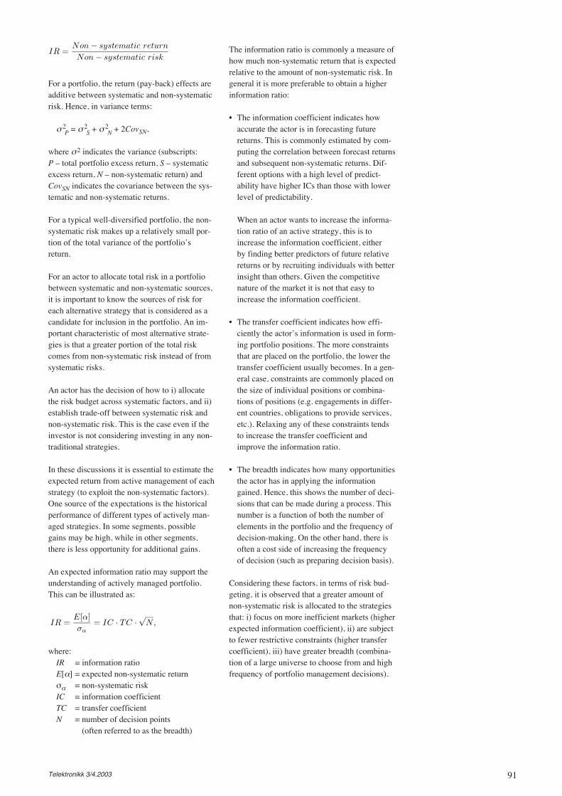
91Telektronikk 3/4.2003
For a portfolio, the return (pay-back) effects areadditive between systematic and non-systematicrisk. Hence, in variance terms:
σ 2P = σ 2
S + σ 2N + 2CovSN,
where σ2 indicates the variance (subscripts:P – total portfolio excess return, S – systematicexcess return, N – non-systematic return) andCovSN indicates the covariance between the sys-tematic and non-systematic returns.
For a typical well-diversified portfolio, the non-systematic risk makes up a relatively small por-tion of the total variance of the portfolio’sreturn.
For an actor to allocate total risk in a portfoliobetween systematic and non-systematic sources,it is important to know the sources of risk foreach alternative strategy that is considered as acandidate for inclusion in the portfolio. An im-portant characteristic of most alternative strate-gies is that a greater portion of the total riskcomes from non-systematic risk instead of fromsystematic risks.
An actor has the decision of how to i) allocatethe risk budget across systematic factors, and ii)establish trade-off between systematic risk andnon-systematic risk. This is the case even if theinvestor is not considering investing in any non-traditional strategies.
In these discussions it is essential to estimate theexpected return from active management of eachstrategy (to exploit the non-systematic factors).One source of the expectations is the historicalperformance of different types of actively man-aged strategies. In some segments, possiblegains may be high, while in other segments,there is less opportunity for additional gains.
An expected information ratio may support theunderstanding of actively managed portfolio.This can be illustrated as:
The information ratio is commonly a measure ofhow much non-systematic return that is expectedrelative to the amount of non-systematic risk. Ingeneral it is more preferable to obtain a higherinformation ratio:
• The information coefficient indicates howaccurate the actor is in forecasting futurereturns. This is commonly estimated by com-puting the correlation between forecast returnsand subsequent non-systematic returns. Dif-ferent options with a high level of predict-ability have higher ICs than those with lowerlevel of predictability.
When an actor wants to increase the informa-tion ratio of an active strategy, this is toincrease the information coefficient, eitherby finding better predictors of future relativereturns or by recruiting individuals with betterinsight than others. Given the competitivenature of the market it is not that easy toincrease the information coefficient.
• The transfer coefficient indicates how effi-ciently the actor’s information is used in form-ing portfolio positions. The more constraintsthat are placed on the portfolio, the lower thetransfer coefficient usually becomes. In a gen-eral case, constraints are commonly placed onthe size of individual positions or combina-tions of positions (e.g. engagements in differ-ent countries, obligations to provide services,etc.). Relaxing any of these constraints tendsto increase the transfer coefficient andimprove the information ratio.
• The breadth indicates how many opportunitiesthe actor has in applying the informationgained. Hence, this shows the number of deci-sions that can be made during a process. Thisnumber is a function of both the number ofelements in the portfolio and the frequency ofdecision-making. On the other hand, there isoften a cost side of increasing the frequencyof decision (such as preparing decision basis).
Considering these factors, in terms of risk bud-geting, it is observed that a greater amount ofnon-systematic risk is allocated to the strategiesthat: i) focus on more inefficient markets (higherexpected information coefficient), ii) are subjectto fewer restrictive constraints (higher transfercoefficient), iii) have greater breadth (combina-tion of a large universe to choose from and highfrequency of portfolio management decisions).
IR =
Non − systematic return
Non − systematic risk
where:IR = information ratioE[α] = expected non-systematic returnσα = non-systematic riskIC = information coefficientTC = transfer coefficientN = number of decision points
(often referred to as the breadth)
IR =E[α]
σα
= IC · TC ·√
N,
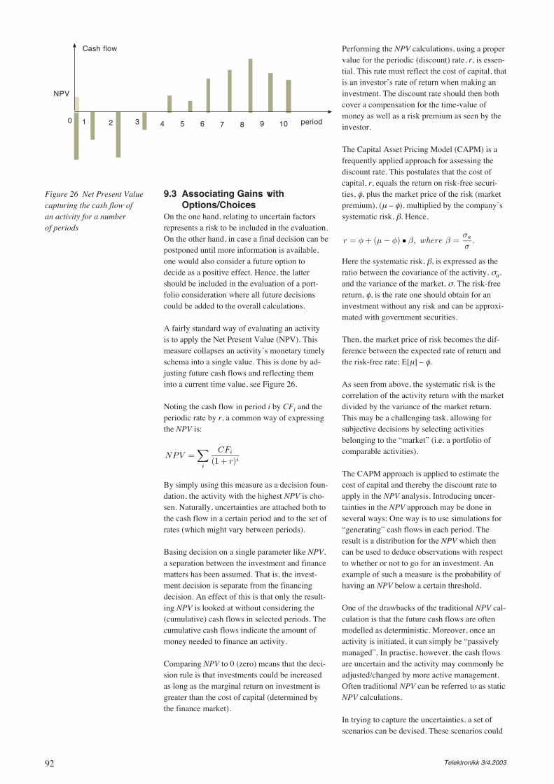
92 Telektronikk 3/4.2003
9.3 Associating Gains withOptions/Choices
On the one hand, relating to uncertain factorsrepresents a risk to be included in the evaluation.On the other hand, in case a final decision can bepostponed until more information is available,one would also consider a future option todecide as a positive effect. Hence, the lattershould be included in the evaluation of a port-folio consideration where all future decisionscould be added to the overall calculations.
A fairly standard way of evaluating an activityis to apply the Net Present Value (NPV). Thismeasure collapses an activity’s monetary timelyschema into a single value. This is done by ad-justing future cash flows and reflecting theminto a current time value, see Figure 26.
Noting the cash flow in period i by CFi and theperiodic rate by r, a common way of expressingthe NPV is:
Performing the NPV calculations, using a propervalue for the periodic (discount) rate, r, is essen-tial. This rate must reflect the cost of capital, thatis an investor’s rate of return when making aninvestment. The discount rate should then bothcover a compensation for the time-value ofmoney as well as a risk premium as seen by theinvestor.
The Capital Asset Pricing Model (CAPM) is afrequently applied approach for assessing thediscount rate. This postulates that the cost ofcapital, r, equals the return on risk-free securi-ties, φ, plus the market price of the risk (marketpremium), (µ – φ), multiplied by the company’ssystematic risk, β. Hence,
Figure 26 Net Present Valuecapturing the cash flow ofan activity for a numberof periods
period1 2 3 4 5 6 7 8 9 10
Cash flow
NPV
0
By simply using this measure as a decision foun-dation, the activity with the highest NPV is cho-sen. Naturally, uncertainties are attached both tothe cash flow in a certain period and to the set ofrates (which might vary between periods).
Basing decision on a single parameter like NPV,a separation between the investment and financematters has been assumed. That is, the invest-ment decision is separate from the financingdecision. An effect of this is that only the result-ing NPV is looked at without considering the(cumulative) cash flows in selected periods. Thecumulative cash flows indicate the amount ofmoney needed to finance an activity.
Comparing NPV to 0 (zero) means that the deci-sion rule is that investments could be increasedas long as the marginal return on investment isgreater than the cost of capital (determined bythe finance market).
NPV =∑
i
CFi
(1 + r)i
Here the systematic risk, β, is expressed as theratio between the covariance of the activity, σa,and the variance of the market, σ. The risk-freereturn, φ, is the rate one should obtain for aninvestment without any risk and can be approxi-mated with government securities.
Then, the market price of risk becomes the dif-ference between the expected rate of return andthe risk-free rate; E[µ] – φ.
As seen from above, the systematic risk is thecorrelation of the activity return with the marketdivided by the variance of the market return.This may be a challenging task, allowing forsubjective decisions by selecting activitiesbelonging to the “market” (i.e. a portfolio ofcomparable activities).
The CAPM approach is applied to estimate thecost of capital and thereby the discount rate toapply in the NPV analysis. Introducing uncer-tainties in the NPV approach may be done inseveral ways; One way is to use simulations for“generating” cash flows in each period. Theresult is a distribution for the NPV which thencan be used to deduce observations with respectto whether or not to go for an investment. Anexample of such a measure is the probability ofhaving an NPV below a certain threshold.
One of the drawbacks of the traditional NPV cal-culation is that the future cash flows are oftenmodelled as deterministic. Moreover, once anactivity is initiated, it can simply be “passivelymanaged”. In practise, however, the cash flowsare uncertain and the activity may commonly beadjusted/changed by more active management.Often traditional NPV can be referred to as staticNPV calculations.
In trying to capture the uncertainties, a set ofscenarios can be devised. These scenarios could
r = φ + (µ − φ) • β, where β =σa
σ.
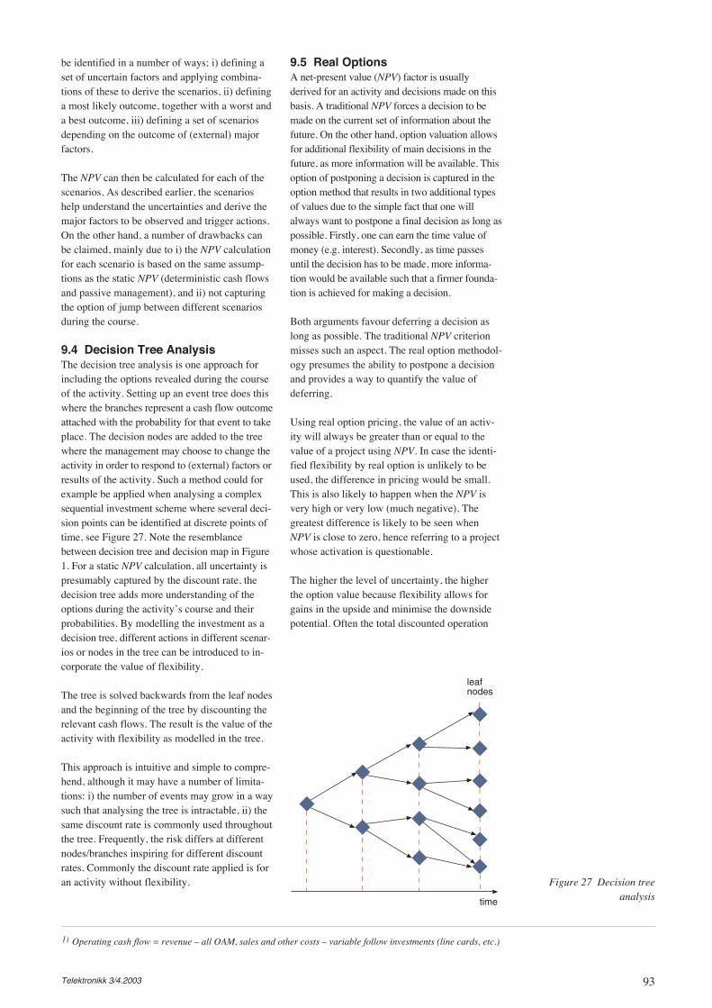
93Telektronikk 3/4.2003
be identified in a number of ways; i) defining aset of uncertain factors and applying combina-tions of these to derive the scenarios, ii) defininga most likely outcome, together with a worst anda best outcome, iii) defining a set of scenariosdepending on the outcome of (external) majorfactors.
The NPV can then be calculated for each of thescenarios. As described earlier, the scenarioshelp understand the uncertainties and derive themajor factors to be observed and trigger actions.On the other hand, a number of drawbacks canbe claimed, mainly due to i) the NPV calculationfor each scenario is based on the same assump-tions as the static NPV (deterministic cash flowsand passive management), and ii) not capturingthe option of jump between different scenariosduring the course.
9.4 Decision Tree AnalysisThe decision tree analysis is one approach forincluding the options revealed during the courseof the activity. Setting up an event tree does thiswhere the branches represent a cash flow outcomeattached with the probability for that event to takeplace. The decision nodes are added to the treewhere the management may choose to change theactivity in order to respond to (external) factors orresults of the activity. Such a method could forexample be applied when analysing a complexsequential investment scheme where several deci-sion points can be identified at discrete points oftime, see Figure 27. Note the resemblancebetween decision tree and decision map in Figure1. For a static NPV calculation, all uncertainty ispresumably captured by the discount rate, thedecision tree adds more understanding of theoptions during the activity’s course and theirprobabilities. By modelling the investment as adecision tree, different actions in different scenar-ios or nodes in the tree can be introduced to in-corporate the value of flexibility.
The tree is solved backwards from the leaf nodesand the beginning of the tree by discounting therelevant cash flows. The result is the value of theactivity with flexibility as modelled in the tree.
This approach is intuitive and simple to compre-hend, although it may have a number of limita-tions: i) the number of events may grow in a waysuch that analysing the tree is intractable, ii) thesame discount rate is commonly used throughoutthe tree. Frequently, the risk differs at differentnodes/branches inspiring for different discountrates. Commonly the discount rate applied is foran activity without flexibility.
9.5 Real OptionsA net-present value (NPV) factor is usuallyderived for an activity and decisions made on thisbasis. A traditional NPV forces a decision to bemade on the current set of information about thefuture. On the other hand, option valuation allowsfor additional flexibility of main decisions in thefuture, as more information will be available. Thisoption of postponing a decision is captured in theoption method that results in two additional typesof values due to the simple fact that one willalways want to postpone a final decision as long aspossible. Firstly, one can earn the time value ofmoney (e.g. interest). Secondly, as time passesuntil the decision has to be made, more informa-tion would be available such that a firmer founda-tion is achieved for making a decision.
Both arguments favour deferring a decision aslong as possible. The traditional NPV criterionmisses such an aspect. The real option methodol-ogy presumes the ability to postpone a decisionand provides a way to quantify the value ofdeferring.
Using real option pricing, the value of an activ-ity will always be greater than or equal to thevalue of a project using NPV. In case the identi-fied flexibility by real option is unlikely to beused, the difference in pricing would be small.This is also likely to happen when the NPV isvery high or very low (much negative). Thegreatest difference is likely to be seen whenNPV is close to zero, hence referring to a projectwhose activation is questionable.
The higher the level of uncertainty, the higherthe option value because flexibility allows forgains in the upside and minimise the downsidepotential. Often the total discounted operation
1) Operating cash flow = revenue – all OAM, sales and other costs – variable follow investments (line cards, etc.)
time
leafnodes
Figure 27 Decision treeanalysis
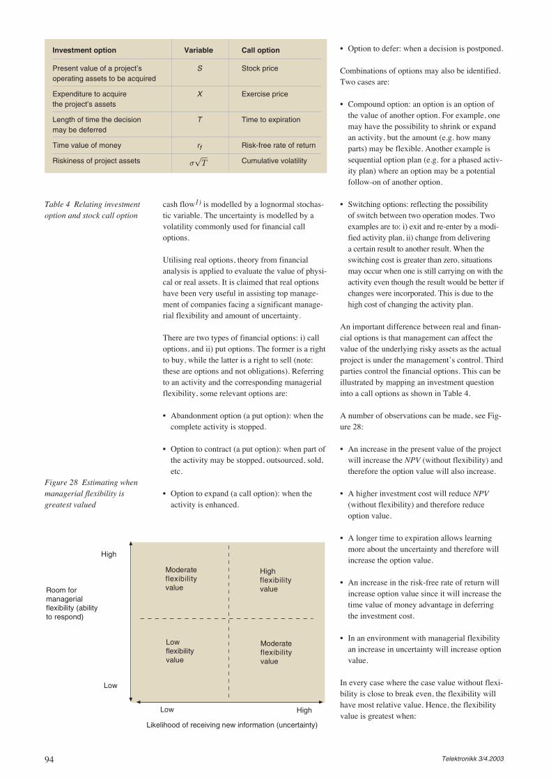
94 Telektronikk 3/4.2003
cash flow1) is modelled by a lognormal stochas-tic variable. The uncertainty is modelled by avolatility commonly used for financial calloptions.
Utilising real options, theory from financialanalysis is applied to evaluate the value of physi-cal or real assets. It is claimed that real optionshave been very useful in assisting top manage-ment of companies facing a significant manage-rial flexibility and amount of uncertainty.
There are two types of financial options: i) calloptions, and ii) put options. The former is a rightto buy, while the latter is a right to sell (note:these are options and not obligations). Referringto an activity and the corresponding managerialflexibility, some relevant options are:
• Abandonment option (a put option): when thecomplete activity is stopped.
• Option to contract (a put option): when part ofthe activity may be stopped, outsourced, sold,etc.
• Option to expand (a call option): when theactivity is enhanced.
• Option to defer: when a decision is postponed.
Combinations of options may also be identified.Two cases are:
• Compound option: an option is an option ofthe value of another option. For example, onemay have the possibility to shrink or expandan activity, but the amount (e.g. how manyparts) may be flexible. Another example issequential option plan (e.g. for a phased activ-ity plan) where an option may be a potentialfollow-on of another option.
• Switching options: reflecting the possibilityof switch between two operation modes. Twoexamples are to: i) exit and re-enter by a modi-fied activity plan, ii) change from deliveringa certain result to another result. When theswitching cost is greater than zero, situationsmay occur when one is still carrying on with theactivity even though the result would be better ifchanges were incorporated. This is due to thehigh cost of changing the activity plan.
An important difference between real and finan-cial options is that management can affect thevalue of the underlying risky assets as the actualproject is under the management’s control. Thirdparties control the financial options. This can beillustrated by mapping an investment questioninto a call options as shown in Table 4.
A number of observations can be made, see Fig-ure 28:
• An increase in the present value of the projectwill increase the NPV (without flexibility) andtherefore the option value will also increase.
• A higher investment cost will reduce NPV(without flexibility) and therefore reduceoption value.
• A longer time to expiration allows learningmore about the uncertainty and therefore willincrease the option value.
• An increase in the risk-free rate of return willincrease option value since it will increase thetime value of money advantage in deferringthe investment cost.
• In an environment with managerial flexibilityan increase in uncertainty will increase optionvalue.
In every case where the case value without flexi-bility is close to break even, the flexibility willhave most relative value. Hence, the flexibilityvalue is greatest when:
Investment option Variable Call option
Present value of a project’s S Stock priceoperating assets to be acquired
Expenditure to acquire X Exercise pricethe project’s assets
Length of time the decision T Time to expirationmay be deferred
Time value of money rf Risk-free rate of return
Riskiness of project assets Cumulative volatility
Table 4 Relating investmentoption and stock call option
Likelihood of receiving new information (uncertainty)
Low High
High
Room formanagerialflexibility (abilityto respond)
Low
Moderateflexibilityvalue
Lowflexibilityvalue
Highflexibilityvalue
Moderateflexibilityvalue
Figure 28 Estimating whenmanagerial flexibility isgreatest valued
σ
√T

95Telektronikk 3/4.2003
• Great uncertainty about the future. Very likelyto receive new information over time.
• Much room for managerial flexibility. Allowsmanagement to respond appropriately to thisnew information.
• NPV without flexibility near zero. If the activ-ity is neither obviously good nor obviouslybad, flexibility to change course is more likelyto be used and is therefore more valuable.
In the financial world, the Black-Scholes for-mula is well-applied for valuing real options.This is an analytical solution to a differentialequation describing the value of a European calloption. The underlying risky asset is assumed tofollow a geometric Brownian Motion with aMarkov-Wiener stochastic process. When S isthe value, the percent change is given by:
to the binomial lattice approaches the time con-tinuous solution of Black-Scholes as the numberof time-steps in the binomial tree gets larger.
The calculations are started from the leaf nodesof the tree (similar to Figure 27) where the ques-tion of whether to exercise the option or not is atrivial one (being the end-points). The calcula-tions are run backwards to the beginning of thetree, choosing the best decision of whether toexercise or not at each branch/node of the tree.At each branch/ node the market-replicatingportfolios or the risk-neutral approach can beapplied, both being equivalent to each other. Theformer refers to finding an equivalent combina-tion of risky and risk-free assets, while the latterrefers to adjusting the cash flows in the NPV cal-culations.
Naturally, one may raise the question of how tofind an equivalent portfolio when referring to anactivity “never-seen-before” for a certain com-pany. On the one hand, it can be claimed thatthese are all models used as background whenmaking the actual decisions. On the other hand,the static NPV of an activity could be used as abest-guess on the unbiased estimate of the mar-ket value of the activity. Considering the valueincluding flexibility, one could consider this asplacing one part of the money on the activity andanother part in bonds.
The binomial event tree describes the evolvinguncertainty of the underlying risky asset and thestochastic process is based on a single volatility.Monte Carlo simulation is commonly used toproduce the volatility for the return of activity.This is however based on the assumption that theuncertainty is resolved continuously over time.There are often different causes for uncertainties,such as market and technology. These may wellbe resolved differently with time; an examplebeing that technological uncertainties decreasewith time while market uncertainties increasewith time.
Figure 29 Potentialcategorisation ofvendor’s strength
0
1
2
3
4Breadth of vision
External expression of vision
Internal expression of vision
Ability to execute
Ability of change direction
Financial stability
δS
S= µ · δt + σ · ε ·
√δt
where
µ is a drift term or growth parameter thatincreases at a factor of time steps δt.
δ is the volatility parameter, growing at a rateof the square root of time.
ε is simulated, usually following a normal distri-bution with a mean of zero and variance of one.
The first term is the deterministic part and thesecond term is the stochastic part.
A number of limitations on this formula are:there is only one source of uncertainty, no com-pound options are included, the underlyingstochastic process is assumed to be known, thevariance of return is constant through time, theunderlying risky asset follows a GeometricBrownian Motion with a Markov-Wienerstochastic process.
One way of modelling real options is to applybinomial lattices. Market-replicating portfoliosand risk-neutral approach could for instance beused when calculating the values of the optionsets. The basic idea is to represent the evolvinguncertainty of the value of a risky asset by abinominal tree. The risk itself may or may notincrease with time, but uncertainty increases withtime. This can be considered as an uncertaintycone (hence growing as time passes). In the sameway as the Black-Scholes formula this relies ona Geometric Brownian Motion following aMarkov-Wiener process. As for any tree, timeis discretised, and hence it may become quitedemanding to compute every combination. As alimit, the value of an option calculated according

96 Telektronikk 3/4.2003
Real Options – Referring to Stocks
One model for stock behaviour is a so-called geometric Brownian motion. The time discreteversion is expressed as:
where:
S(t) – stock price at time t
∆S(t) – change in stock price during a short time interval, ∆t
rf – drift rate (risk-free rate of return)
σ – volatility
ε – random number drawn from a standard normal distribution (~N(0,1)).
Now it can be shown that S(t) is log normally distributed with mean value given as
and standard deviation of
The measure under consideration, here the total discounted value of the operating cash flow of aproject, T, is estimated at S(0) with the current information. Up to decision time, T, the manage-ment receives information of relevant value and the measure value will therefore move up ordown with accumulated volatility .
The project investment is only incurred if S(T) > X’’ = X + (1 + rD)2V, where X is the initialinvestment at time T and V is the NPV of the second phase of the project if the uncertain actionis not carried out. rD is the discount rate.
The NPV at time T is found as:
where
After some reordering and variable substitution (e.g. w = ln(S(t)) -> S(T) = ew, dS(t) = ewdw),one gets
NPV = e–rfT (S N(d1)erfT – X N(d2)) + V (1 – N(d2))
where
and
N(.) is the cumulative standard normal distribution (~N(0,1)).
9.6 Stochastic OptimisationStochastic optimisation is an operationalresearch technique for handling uncertainty. Thisis applied in order to optimise simulation modelsby defining a stochastic model and accompany-ing decision variables. Iterations are carried outbetween drawing input parameters from selecteddistributions and optimising the decision vari-ables for each set of draws. In some sense thisis similar to solving the task of finding the bestpath in a decision tree.
9.7 Evaluating VendorsOne element in the risk assessment is evaluatingthe situation of the current vendors. Both techni-cal and financial criteria have to be considered.
Having an assessment of the key vendors for anoperator is also central. Several criteria could bederived, of which some are (from [Heav03]):
• Breadth of vision• External expression of vision• Internal expression of vision
∆S(t)
S(t)= rf∆t + σε
√∆t
µt = ln(S(0)) +
(rf −
σ2
2
)t
σt = σ
√t.
σ
√t
NPV = E[max(S(T ) − X, (1 + rD)2V )
]
=
∫∞
X′′
(S(T ) − X)p(S(T ))dS(T ) +
∫X
′′
0
(1 + rD)2V p(S(T ))dS(T )
p(S(T )) =1
σT
√2πS(T )
e
−(ln(S(T ))−µT )2
2σ2T
d1 =
ln(
SX′′
)+
(rf +
σ2
2
)T
σ√
T
d2 =
ln(
SX′′
)+
(rf − σ2
2
)T
σ√
T= d1 − σ
√T .
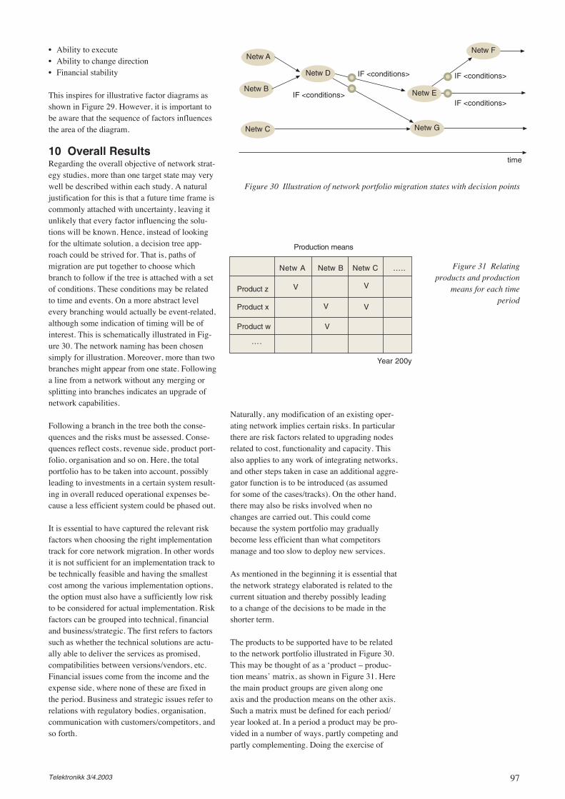
97Telektronikk 3/4.2003
• Ability to execute• Ability to change direction • Financial stability
This inspires for illustrative factor diagrams asshown in Figure 29. However, it is important tobe aware that the sequence of factors influencesthe area of the diagram.
10 Overall ResultsRegarding the overall objective of network strat-egy studies, more than one target state may verywell be described within each study. A naturaljustification for this is that a future time frame iscommonly attached with uncertainty, leaving itunlikely that every factor influencing the solu-tions will be known. Hence, instead of lookingfor the ultimate solution, a decision tree app-roach could be strived for. That is, paths ofmigration are put together to choose whichbranch to follow if the tree is attached with a setof conditions. These conditions may be relatedto time and events. On a more abstract levelevery branching would actually be event-related,although some indication of timing will be ofinterest. This is schematically illustrated in Fig-ure 30. The network naming has been chosensimply for illustration. Moreover, more than twobranches might appear from one state. Followinga line from a network without any merging orsplitting into branches indicates an upgrade ofnetwork capabilities.
Following a branch in the tree both the conse-quences and the risks must be assessed. Conse-quences reflect costs, revenue side, product port-folio, organisation and so on. Here, the totalportfolio has to be taken into account, possiblyleading to investments in a certain system result-ing in overall reduced operational expenses be-cause a less efficient system could be phased out.
It is essential to have captured the relevant riskfactors when choosing the right implementationtrack for core network migration. In other wordsit is not sufficient for an implementation track tobe technically feasible and having the smallestcost among the various implementation options,the option must also have a sufficiently low riskto be considered for actual implementation. Riskfactors can be grouped into technical, financialand business/strategic. The first refers to factorssuch as whether the technical solutions are actu-ally able to deliver the services as promised,compatibilities between versions/vendors, etc.Financial issues come from the income and theexpense side, where none of these are fixed inthe period. Business and strategic issues refer torelations with regulatory bodies, organisation,communication with customers/competitors, andso forth.
Naturally, any modification of an existing oper-ating network implies certain risks. In particularthere are risk factors related to upgrading nodesrelated to cost, functionality and capacity. Thisalso applies to any work of integrating networks,and other steps taken in case an additional aggre-gator function is to be introduced (as assumedfor some of the cases/tracks). On the other hand,there may also be risks involved when nochanges are carried out. This could comebecause the system portfolio may graduallybecome less efficient than what competitorsmanage and too slow to deploy new services.
As mentioned in the beginning it is essential thatthe network strategy elaborated is related to thecurrent situation and thereby possibly leadingto a change of the decisions to be made in theshorter term.
The products to be supported have to be relatedto the network portfolio illustrated in Figure 30.This may be thought of as a ‘product – produc-tion means’ matrix, as shown in Figure 31. Herethe main product groups are given along oneaxis and the production means on the other axis.Such a matrix must be defined for each period/year looked at. In a period a product may be pro-vided in a number of ways, partly competing andpartly complementing. Doing the exercise of
time
Netw A
Netw B
Netw C
Netw F
IF <conditions>
IF <conditions>IF <conditions>
IF <conditions>
Netw G
Netw E
Netw D
Figure 30 Illustration of network portfolio migration states with decision points
Production means
Netw A
Product z
Product x
Product w
Netw B Netw C …..
….
V
V
V
V
V
Year 200y
Figure 31 Relatingproducts and production
means for each timeperiod
98 Telektronikk 3/4.2003
relating products to production means will revealfurther areas of potential gains.
To some extent products to be supported havebeen described earlier. A few basic trends havealso been outlined earlier. Regarding the demandpatterns, most sources indicate a growth in mostissues, leading to rather questionable aggregateddemands. However, trends showing main growthareas within mobile, IP and xDLS are repeatedlyobserved.
Defining how to efficiently support the differentproducts belongs to the network portfolio man-agement. A basic challenge is to relate the ser-vices and market segments. An example of howthis may be carried out is depicted in Figure 32.
11 Concluding RemarksA network strategy is needed for every soundnetwork operation. The strategy must also berelated to decisions and actions in near-time –hence, the strategy must be made operational.A main goal of having a strategy is to be pre-pared for chances that can be revealed duringthe course of events. That is, the strategy islikely to assist when detecting business opportu-nities. The total network portfolio must beincluded, also seeing synergies between the dif-ferent systems in the shorter and longer terms.
In elaborating the strategy a number of methodscan be applied, including scenarios, cost/benefitcalculations and risk assessment. A descriptionof various aspects is outlined in this article.
AcknowledgementAlthough the material in this text is the soleresponsibility of the author, fruitful discussionswith all colleagues involved in Telenor strategywork in later years are appreciated.
References[Cari01] Canadian Treasury Board. IntegratedRisk Management Framework. 2001. Online:http://www.tbs-sct.gc.ca
[Heav03] Heavy Reading: Incumbents’ wirelinestrategies, 1 (3), 2003.
Figure 32 Example of relatingservices/customer segments toproduction means (Note: notall relevant systems areincluded, e.g. the mobilesystems)
VoiceDial - up IP
Residential tolarge enterprises CU LE TE TE LE Cu
ISDN/PSTN
VoiceIP
Residential,SoHo,SME
xDSL
xDSL
Sw
ATM IP
ISPs
xDSL WDMSMEHSDSL HSDSLWDM
Large enterpriseSDH
SDH
CU - Concentration UnitLE - Local ExchangeTE - Transit ExchangeSw - SwitchR - Router
VoiceLL
LL
xx
SDH
xDSL
R
Services Customers
99
1 IntroductionPrinciples for evaluation of the risk associatedwith a portfolio of investment projects withina company are based on models that describepotential changes in the factors that influence theprofit of the individual projects and the interac-tion between these. Many different models aredescribed in the literature. Some approaches aresimple and may border towards the trivial, whilstothers are more involved and rely on advancedstochastic models. During the last years it hasbecome popular to apply principles and theoryfrom the mathematics of finance (see e.g. [1] and[2]). Analogy is drawn between investment insecurities on the one hand and investment inprojects on the other. Both situations are charac-terised by the investment of an amount of moneyat one or several points in time with the hope ofreceiving larger sums of money at one or morefuture points in time. Such analogy has its strongand weak sides.
In this paper we describe an approach based onwhat we call Risk-Adjusted Expected Net Pre-sent Value (RAENPV) and contrast it to the morecommon Net Present Value (NPV) with RiskAdjusted Discount Rate. We also propose a wayof describing the uncertainty associated with thecash flow of each individual candidate project ina portfolio and how it interacts with each of theother candidate projects. Our guiding principlehas been to establish an approach, which on theone hand is not too narrow but on the other handavoids relying on complicated models that can-not be justified because of lack of knowledgeabout the future.
2 Evaluation of a SingleProject
2.1 Risk-adjusted Discount RateWe shall first briefly comment in general termson an approach which is often used where aproject is rated according to its NPV calculatedusing a risk-adjusted discount rate that reflectsthe uncertainties in the cash flow. The approachis usually based on variants of the Capital AssetPricing Model (CAPM). A thorough descriptionof CAPM may be found in [1]. A feature of thisapproach is that high uncertainty in the cashflow leads to a high risk-adjusted discount rate.The approach is not without problems, even forprojects with a lifetime of one period only.We mention some of the conditions that mustbe satisfied:
• Investors have expectations about assetreturns that are normally distributed.
• Investors may borrow or lend unlimitedamounts of a risk-free asset.
• All projects (and parts of projects) can bebought/sold in a perfect market.
Even stronger are the conditions that must besatisfied if we want to use a risk-adjusted dis-count rate for projects with a lifetime of morethan one period. Then it must be assumed thatthe cash flow in one period is a deterministicfunction of the cash flow in the previous periodplus a random variable that is independent ofwhat has happened in all previous periods.
2.2 Problems with the Use of aRisk-adjusted Discount Rate– Examples
In many situations it is not reasonable to assumethat the conditions mentioned in the previoussection are satisfied. We shall show by threeproject examples what happens when theseconditions are not fulfilled. The examples arestylised to visualise the effect of risk-adjustingthe discount rate. However, their basic featuresare not unrealistic.
The cost of capital is assumed to be 12 %, andwe assume that the relevant risk-adjusted dis-count rate has been found (using for exampleCAPM type arguments) to be 13 % for all threeprojects. All amounts are in millions of dollars.
Example 1:We invest 98 in year 0 in building a VDSL access
network. There is uncertainty as to whether the
revenue from subscribers will commence in year
1 or 2. With probability 1/2 we receive a net
income of 13 in year 1. In the years 2, 3, … we
receive with probability 1 a yearly net income of
13. The uncertainty is thus whether the income
stream starts in year 1 or 2 (see Figure 1 where
the income that occurs with probability 1/2 is
hatched).
Situation A – Net income 13 in year 1:The NPV becomes (13/1.12) / (1 – 1/1.12) – 98
= 10.3.
Situation B – Net income 0 in year 1:The NPV becomes (13/1.122) / (1 – 1/1.12) – 98
= –1.3.
Portfolio Evaluation Under UncertaintyR A L P H L O R E N T Z E N
Ralph Lorentzen (67) is dailyleader of the companyLorentzen LP Service whichdoes consulting work withinmathematical programming. Heretired July 1, 2003 from his jobas senior scientist in TelenorR&D. Ralph Lorentzen gradu-ated in mathematics at the Uni-versity of Oslo, where heworked for some time as assis-tant professor giving lectures instatistics and operationsresearch. He worked as distribu-tion planner in Norske Esso, asprincipal scientist at ShapeTechnical Centre, as systemsengineer in IBM, and as chiefconsultant in Control Data Nor-way, before joining Telenor R&Din 1985.
Telektronikk 3/4.2003
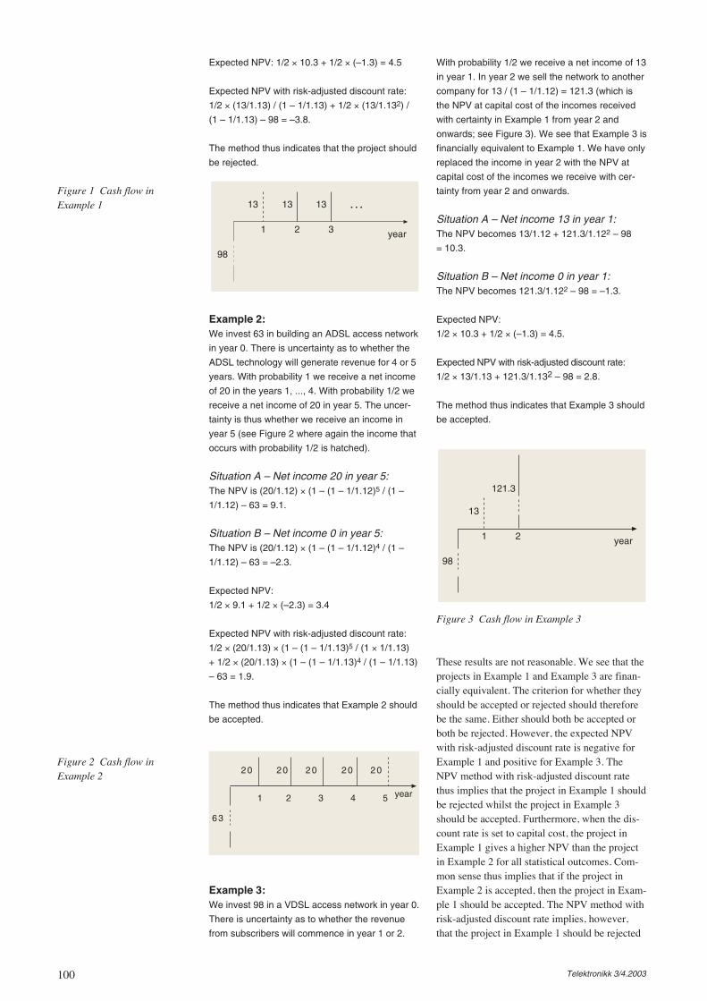
100 Telektronikk 3/4.2003
Expected NPV: 1/2 × 10.3 + 1/2 × (–1.3) = 4.5
Expected NPV with risk-adjusted discount rate:
1/2 × (13/1.13) / (1 – 1/1.13) + 1/2 × (13/1.132) /
(1 – 1/1.13) – 98 = –3.8.
The method thus indicates that the project should
be rejected.
With probability 1/2 we receive a net income of 13
in year 1. In year 2 we sell the network to another
company for 13 / (1 – 1/1.12) = 121.3 (which is
the NPV at capital cost of the incomes received
with certainty in Example 1 from year 2 and
onwards; see Figure 3). We see that Example 3 is
financially equivalent to Example 1. We have only
replaced the income in year 2 with the NPV at
capital cost of the incomes we receive with cer-
tainty from year 2 and onwards.
Situation A – Net income 13 in year 1:The NPV becomes 13/1.12 + 121.3/1.122 – 98
= 10.3.
Situation B – Net income 0 in year 1:The NPV becomes 121.3/1.122 – 98 = –1.3.
Expected NPV:
1/2 × 10.3 + 1/2 × (–1.3) = 4.5.
Expected NPV with risk-adjusted discount rate:
1/2 × 13/1.13 + 121.3/1.132 – 98 = 2.8.
The method thus indicates that Example 3 should
be accepted.
Figure 1 Cash flow inExample 1
Figure 2 Cash flow inExample 2
Figure 3 Cash flow in Example 3
…13 13 13
1 32
98
year
Example 2:We invest 63 in building an ADSL access network
in year 0. There is uncertainty as to whether the
ADSL technology will generate revenue for 4 or 5
years. With probability 1 we receive a net income
of 20 in the years 1, ..., 4. With probability 1/2 we
receive a net income of 20 in year 5. The uncer-
tainty is thus whether we receive an income in
year 5 (see Figure 2 where again the income that
occurs with probability 1/2 is hatched).
Situation A – Net income 20 in year 5:The NPV is (20/1.12) × (1 – (1 – 1/1.12)5 / (1 –
1/1.12) – 63 = 9.1.
Situation B – Net income 0 in year 5:The NPV is (20/1.12) × (1 – (1 – 1/1.12)4 / (1 –
1/1.12) – 63 = –2.3.
Expected NPV:
1/2 × 9.1 + 1/2 × (–2.3) = 3.4
Expected NPV with risk-adjusted discount rate:
1/2 × (20/1.13) × (1 – (1 – 1/1.13)5 / (1 × 1/1.13)
+ 1/2 × (20/1.13) × (1 – (1 – 1/1.13)4 / (1 – 1/1.13)
– 63 = 1.9.
The method thus indicates that Example 2 should
be accepted.
63
20 2020
1 2 3 4 5 year
2020
year
13
1 2
98
121.3
These results are not reasonable. We see that theprojects in Example 1 and Example 3 are finan-cially equivalent. The criterion for whether theyshould be accepted or rejected should thereforebe the same. Either should both be accepted orboth be rejected. However, the expected NPVwith risk-adjusted discount rate is negative forExample 1 and positive for Example 3. TheNPV method with risk-adjusted discount ratethus implies that the project in Example 1 shouldbe rejected whilst the project in Example 3should be accepted. Furthermore, when the dis-count rate is set to capital cost, the project inExample 1 gives a higher NPV than the projectin Example 2 for all statistical outcomes. Com-mon sense thus implies that if the project inExample 2 is accepted, then the project in Exam-ple 1 should be accepted. The NPV method withrisk-adjusted discount rate implies, however,that the project in Example 1 should be rejected
Example 3:We invest 98 in a VDSL access network in year 0.
There is uncertainty as to whether the revenue
from subscribers will commence in year 1 or 2.
101Telektronikk 3/4.2003
whilst the project in Example 2 should beaccepted.
The examples demonstrate that any methodbased on risk-adjusting the discount rate isunable to differentiate correctly between differ-ent risk structures. By risk-adjusting the discountrate one tries to satisfy two masters. The discountrate should reflect
• Capital cost (i.e. the rate of return which canbe achieved by alternative application of themoney which are tied up/released in the pro-ject over time). This has nothing to do withthe risk of the project under consideration;
• The risk associated with the project
These two requirements are fundamentally dif-ferent, and it is difficult to satisfy both by adjust-ing the discount rate. The main reason to lookfor an alternative approach is to be able to differ-entiate between capital cost and risk.
2.3 Risk-adjusted Expected NetPresent Value
We shall now describe our suggested approach.The expected NPV is calculated using capitalcost w as discount rate. The capital cost shouldreflect the average expected rate of return foralternative projects in the company and hasnothing to do with the risk associated with theproject under evaluation.
Then an amount is subtracted from the expectedNPV. This amount adjusts the Expected NPVbecause of the risk of the project. The suggestedmeasure of utility of a project is
Expected NPV – α × risk (2.3.1)
where α is a parameter to be determined. Infinancial theory the risk is traditionally ex-pressed through the standard deviation of theNPV. This is a reasonable measure for portfoliosof securities. Such portfolios consist of a numberof different securities, and the return is the sumof the returns of the individual securities. Thecentral limit theorem in probability theory indi-cates that this sum is approximately normallydistributed. Risk should reflect the down side ofthe distribution of the NPV. However, the nor-mal distribution is symmetric, so the standarddeviation expresses the down side as well as theup side of the distribution. For individual invest-ment projects in a company the assumption thatthe NPV has a symmetric probability distribu-tion is obviously unreasonable. The NPV willoften have a skewed distribution. As the stan-dard deviation also reflects the up side of thedistribution, we may have a large standard de-viation even if the risk of the project is small.
Therefore we choose to measure risk by usingthe well-known concept Value-at-Risk at q(VaRq). VaRq is defined as the q-point in theprobability distribution of the NPV (see Figure4).
q is usually chosen to be 1 % or 5 %. The sug-gested RAENPV then becomes
Expected NPV – α × (–VaRq) (2.3.2)
where the NPV is calculated using the capitalcost w as discount rate and where the parameterα reflects how the company (or its shareholders)weigh expected profit versus risk. We shall seelater that the term – α × (–VaRq) can be inter-preted as the insurance premium the company iswilling to pay in order to be guaranteed against anegative NPV.
We shall now show how we determine α. For aperfect security market which contains a risk-free asset it is established knowledge that thesubstitution rate γ (price of risk) between ex-pected return and risk (measured by the standarddeviation of the return) in equilibrium is thesame for all investors independent of their will-ingness to take risk (see e.g. [1] chapter 6). Thevalue of γ can be obtained from stock exchangedata and is not specific for a particular industrialsector. So for any investor an increment ∆σ inrisk needs to be compensated by an increment of∆σ/γ in expected return. This is shown in [1] forinvestments in a portfolio of securities where theportfolio is sold after one period, but it seemsreasonable to use the same trade-off for multi-period projects. It is reasonable to measure theutility of an investment in a portfolio of securi-ties by E – γσ where E is expected return and σis the standard deviation of the return.
Figure 5 shows the classical picture where thedots represent securities in a diagram with thestandard deviation of the return along the horizon-tal axis and the expected return along the verticalaxis. The lower curve – the opportunity set bordercurve – limits all possible portfolios of securities.The straight line which starts at the risk-free assetand is tangent to the opportunity set border curveis the so-called capital budget line.
Figure 4 Value-at-Risk
Prob. density
q
VaRq 0 NPV
102 Telektronikk 3/4.2003
The point where the capital budget line touchesthe opportunity set border curve represents themarket portfolio and is marked by a small squarein Figure 5. The upper curve in Figure 5 repre-sents an indifference curve for an investor. Thepoint where this curve touches the capital budgetline, and which is marked by a small circle, rep-resents the combination of the market portfolioand the risk-free asset which is considered to beoptimal for this particular investor.
Figure 5 can be transformed to Figure 6 wherewe have replaced the standard deviation of thereturn by –Value-at-Risk for the NPV based on
a discount rate r and the expected return by theexpected NPV.
The rate of increase γ in Figure 5 has here beentransformed to the rate of increase α in Figure 6.It can be shown (see the Appendix) that α isindependent of which discount rate r weapply. We note further that the indifferencecurve for any investor has rate of increase equalto α at the point where it touches the trans-formed capital budget line. That is, α representsthe optimal weighting between expected NPVand –Value-at-Risk. As mentioned earlier, therate of increase γ can be found from capital mar-ket data. The formula for calculating α from γis derived in the Appendix and is
(2.3.3)
where nq is the (1 – q)-point in the standardisednormal distribution.
Since the market portfolio can be regarded asa yardstick, it is of interest to calculate theRAENPV for the market portfolio. In the Ap-pendix it is shown that it can be expressed as
(2.3.4)
where i is the internal rate of return for the mar-ket portfolio.
A project should then be accepted if theRAENPV is greater than this. That will be in theinterest of the shareholders. The project can thenbe represented by a point in Figure 6 that liesabove the transformed capital market line. If theproject is considered as a new investment possi-bility in the capital market, a larger opportunityset, a new transformed capital market line, andhence an improved market portfolio would arise.In Figure 7 the new opportunity set, capital mar-ket line, and market portfolio are indicated bybroken lines. The new market portfolio wouldnecessarily include the project.
An investment possibility represented by a pointunderneath the transformed capital market linemight still improve the revised market portfolioand thus be a profitable investment. This would,however, be rather difficult to ascertain in gen-eral. We therefore propose to be conservativeand leave to the planner the decision whethera project with a negative RAENPV should beaccepted or not.
2.4 Analysis of the Examples UsingRisk-adjusted Net Present Value
We shall now apply our criterion on the threeexamples described earlier where we assumethat a has been estimated to be 0.2 and that theRAENPV of the market portfolio is very small.
Figure 7 Project with higherrisk-adjusted NPV than themarket portfolio
Figure 5 The capital budget line
Figure 6 Transformed capitalbudget line
α
αf
1
γ
σ
α
1
N
Nf
-VaRq
N
Nf
-VaRq
New project
New market portfolio
α =
γ
nq − γ
i − r
(1 + r)(1 − γ/nq)
103Telektronikk 3/4.2003
In all three examples VaRq at capital cost is thesame whether q is 1 % or 5 % since the probabil-ity distributions of the NPV are different fromzero for two values only, and for those valuesthe probabilities are equal to 50 %.
Example 1:The expected NPV and VaRq with discount rate
equal to capital cost are 4.5 and –1.3 respective-
ly. The RAENPV becomes 4.5 – 0.2 × 1.3 = 4.24.
The project should therefore be accepted.
Example 2:The expected NPV and VaRq with discount rate
equal to capital cost are 3.4 and –2.3 respective-
ly. The RAENPV becomes 3.4 – 0.2 × 2.3 = 2.94.
The project should therefore be accepted. We
see that the RAENPV is less than for the project
in Example 1, which is reasonable since the pro-
ject in Example 1 has a higher NPV at capital cost
than the project in Example 2 under both statisti-
cal outcomes.
Example 3:The expected NPV and VaRq with discount rate
equal to capital cost are 4.5 and –1.3 respec-
tively. The RAENPV becomes 4.5 – 0.2 × 1.3 =
4.24. The project should therefore be accepted.
The RAENPV is the same as for the project in
Example 1, which is logical since the two projects
are financially equivalent.
2.5 Establishing the necessary Datafor Evaluation of a Single Project
The cash flow of a project is considered as astochastic process. For every realisation of theprocess the NPV with capital cost as the dis-count rate can be calculated. This NPV is thus arandom variable, and we propose the followingprocedure for estimating its probability distribu-tion.
1 Establish a finite set of alternative future sce-narios and assign a subjective probability ofoccurrence for each scenario.
2 For each scenario establish a pessimistic, anoptimistic and a most probable cash flow forthe project and calculate the NPV for each ofthose three realisations.
3 For each scenario specify an interval aroundthe most probable realisation in which theNPV supposedly will lie with probability 1/2.
4 Fit a Beta distribution to the NPV for eachscenario. Based on the mixture of these Betadistributions using the scenario probabilities,calculate the RAENPV.
Based on the resulting probability distribution ofthe NPV N one can calculate project characteris-tics like:
• Expected NPV (EN)• Value at risk at q (VaRq(N))• Standard deviation (σ(N))• Risk-adjusted ENPV (EN – α(–VaRp(N)))
Example 4:We assume a single scenario. Based on a de-
tailed analysis of the elements contributing to the
cash flow the pessimistic and the optimistic esti-
mates of the NPV for this scenario have been
evaluated to be –400 and 300 respectively, and
the most probable NPV is evaluated to be –100.
The NPV is assumed to lie in the interval (-200, 0)
with probability 1/2. (All figures are in mill. USD.)
The Beta distribution fit gives an expected NPV
equal to –82.5 with standard deviation 134.4. The
probability that the NPV is negative becomes 0.72
and VaR5% becomes –296. If α = .2, the
RAENPV becomes –82.5 – .2 × 296 = –141.7.
3 Evaluation of ProjectPortfolios
3.1 Project Portfolio AlternativesWe shall consider the situation where we havea series of mutually exclusive portfolio alterna-tives. If we have n projects, there are in principleup to 2n portfolio alternatives. In practice thenumber of alternatives will be much lower. Typ-ically, some projects can be started only if someother projects are also started. Similarly theremay be projects that cannot be part of the sameportfolio. The planner must specify such restric-tions, and a planning tool must facilitate thespecification of such restrictions.
3.2 ScenariosWe can specify scenarios for project portfoliosin two alternative ways:
• We can specify scenario alternatives across allprojects.
• We can specify scenario alternatives for eachindividual project.
The two ways are in principle equivalent. If wefor each project p specify the mutually exclusivescenarios , we can definescenarios of the formwhich run across projects. We shall in the sequelassume that the scenarios are defined across theprojects.
∏k(p)
(Si1
1∩ S
i2
2∩ L ∩ S
in
n)
S1p , K, Sk(p)
p
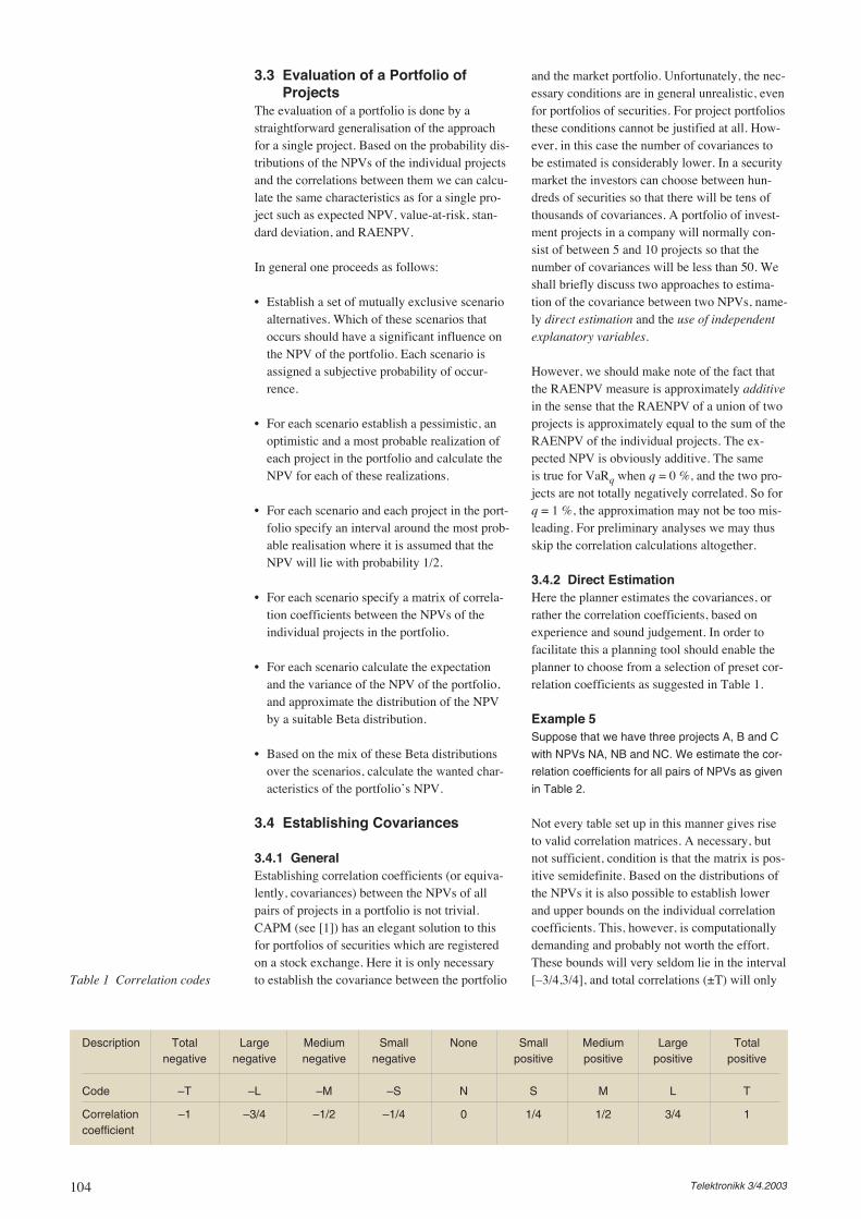
104 Telektronikk 3/4.2003
3.3 Evaluation of a Portfolio ofProjects
The evaluation of a portfolio is done by astraightforward generalisation of the approachfor a single project. Based on the probability dis-tributions of the NPVs of the individual projectsand the correlations between them we can calcu-late the same characteristics as for a single pro-ject such as expected NPV, value-at-risk, stan-dard deviation, and RAENPV.
In general one proceeds as follows:
• Establish a set of mutually exclusive scenarioalternatives. Which of these scenarios thatoccurs should have a significant influence onthe NPV of the portfolio. Each scenario isassigned a subjective probability of occur-rence.
• For each scenario establish a pessimistic, anoptimistic and a most probable realization ofeach project in the portfolio and calculate theNPV for each of these realizations.
• For each scenario and each project in the port-folio specify an interval around the most prob-able realisation where it is assumed that theNPV will lie with probability 1/2.
• For each scenario specify a matrix of correla-tion coefficients between the NPVs of theindividual projects in the portfolio.
• For each scenario calculate the expectationand the variance of the NPV of the portfolio,and approximate the distribution of the NPVby a suitable Beta distribution.
• Based on the mix of these Beta distributionsover the scenarios, calculate the wanted char-acteristics of the portfolio’s NPV.
3.4 Establishing Covariances
3.4.1 GeneralEstablishing correlation coefficients (or equiva-lently, covariances) between the NPVs of allpairs of projects in a portfolio is not trivial.CAPM (see [1]) has an elegant solution to thisfor portfolios of securities which are registeredon a stock exchange. Here it is only necessaryto establish the covariance between the portfolio
and the market portfolio. Unfortunately, the nec-essary conditions are in general unrealistic, evenfor portfolios of securities. For project portfoliosthese conditions cannot be justified at all. How-ever, in this case the number of covariances tobe estimated is considerably lower. In a securitymarket the investors can choose between hun-dreds of securities so that there will be tens ofthousands of covariances. A portfolio of invest-ment projects in a company will normally con-sist of between 5 and 10 projects so that thenumber of covariances will be less than 50. Weshall briefly discuss two approaches to estima-tion of the covariance between two NPVs, name-ly direct estimation and the use of independentexplanatory variables.
However, we should make note of the fact thatthe RAENPV measure is approximately additivein the sense that the RAENPV of a union of twoprojects is approximately equal to the sum of theRAENPV of the individual projects. The ex-pected NPV is obviously additive. The sameis true for VaRq when q = 0 %, and the two pro-jects are not totally negatively correlated. So forq = 1 %, the approximation may not be too mis-leading. For preliminary analyses we may thusskip the correlation calculations altogether.
3.4.2 Direct EstimationHere the planner estimates the covariances, orrather the correlation coefficients, based onexperience and sound judgement. In order tofacilitate this a planning tool should enable theplanner to choose from a selection of preset cor-relation coefficients as suggested in Table 1.
Example 5Suppose that we have three projects A, B and C
with NPVs NA, NB and NC. We estimate the cor-
relation coefficients for all pairs of NPVs as given
in Table 2.
Not every table set up in this manner gives riseto valid correlation matrices. A necessary, butnot sufficient, condition is that the matrix is pos-itive semidefinite. Based on the distributions ofthe NPVs it is also possible to establish lowerand upper bounds on the individual correlationcoefficients. This, however, is computationallydemanding and probably not worth the effort.These bounds will very seldom lie in the interval[–3/4,3/4], and total correlations (±T) will only
Description Total Large Medium Small None Small Medium Large Totalnegative negative negative negative positive positive positive positive
Code –T –L –M –S N S M L T
Correlation –1 –3/4 –1/2 –1/4 0 1/4 1/2 3/4 1coefficient
Table 1 Correlation codes

105Telektronikk 3/4.2003
Using (3.4.6) and (3.4.7) we can find an expres-sion for cov(N1, N2). Analogously we may findformulas for var Np for relevant portfolios p.
Example 6N1 = 10V1 + V2N2 = 2V1 – 3V2
where V1 is Beta distributed over (0,1) with
parameters µn1= 3 and νn1
= 6, whilst V2 is Beta
distributed over (0,1) with parameters µn2= 4 and
νn2= 2, and where V1 and V2 are independent.
Then
We may approximate the distributions of N1 and
N2 by Beta distributions. The intervals are deter-
mined by:
aN1= 0, bN1
= 11, aN2= –3, bN2
= 2.
In order to find the parameters we normalize N1and N2:
This gives
NB NC
NA M –L
NB –S
Table 2 Specification ofcorrelations
be used when the NPVs are linearly dependent.Then the bounds will be –1 and +1 and thus bewithout value.
If the planner has set up a correlation matrixwhich is not positive semidefinite, the planningtool should be able to suggest a modified corre-lation matrix which is positive semidefinite.
3.4.3 Use of Independent ExplanatoryVariables
We assume that we can write the NPVs N1 andN2 for two investment projects 1 and 2 as func-tions of F independent random variables V1, V2,..., VF with known distributions:
Np = Np(V1, V2, ..., VF) for p = 1,2. (3.4.1)
The V-s are explanatory variables which deter-mine e.g. equipment costs, total markets, andmarket shares. Furthermore, we assume that thefunctions Np can be approximated by generalisedpolynomials:
(3.4.2)
where i1, ..., iF may take a finite number of inte-ger values which are not necessarily positive.We are then able to calculate the covariancebetween N1 and N2:
cov(N1, N2) = E(N1N2) – EN1EN2 (3.4.3)
where
(3.4.4)
and
(3.4.5)
such that
(3.4.6)
We assume furthermore that Vf is normalized tolie between 0 and 1 and is Beta distributed withparameters µf and νf. Then
(3.4.7)
Np(V1, V2, K, VF ) ≈
∑
i1,K,iF
αp
i1KiFV
i11
KViF
F
E(N1N2) =
∑
i1,K,iF
j1,K,jF
α1i1KiF
α2j1KjF
EVi1+j11 KEV
iF +jF
F
EN1EN2 =
∑
i1,K,iF
j1,K,jF
α1
i1KiFα
2
j1KjFEV
i11
EVj11
KEViF
F EVjF
F
cov(N1, N2) =∑
i1,K,iF
j1,K,jF
α1
i1KiFα2
j1KjF
(EVi1+j11 KEV
iF +jF
F − EVi11 EV
j11 KEV
iF
F EVjF
F )
EV if =
Γ(µf + νf )Γ(µf + i)
Γ(νf )Γ(µf + νf + i)
EV1 =6
3 + 6=
2
3, EV2 =
2
2 + 4=
1
3
varV1 =3 × 6
(3 + 6)2(3 + 6 + 1)=
1
45,
varV2 =4 × 2
(4 + 2)2(4 + 2 + 1)=
2
63,
cov(N1, N2) = cov(10V1 + V2, 2V1 − 3V2)
= 20varV1 − 3varV2 =22
63
EN1 = 10EV1 + EV2 = 7,
EN2 = 2EV1 − 3EV2 =1
3
varN1 = 100varV1 + varV2 =142
63,
varN2 = 4varV1 + 9varV2 =118
315.
N1 =N1
11, EN1 =
7
11, varN1 =
142
7623,
N2 =N2 + 3
5, EN2 =
2
3, varN2 =
118
7875.
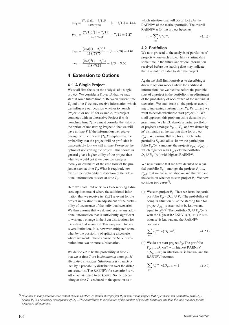
106 Telektronikk 3/4.2003
4 Extension to Options
4.1 A Single ProjectWe shall first focus on the analysis of a singleproject. We consider a Project A that we maystart at some future time T. Between current timeT0 and time T we may receive information whichcan influence our decision whether to launchProject A or not. If, for example, this projectcompetes with an alternative Project B withlaunching time T0, we must consider the value ofthe option of not starting Project A that we willhave at time T. If the information we receiveduring the time interval [T0,T] implies that theprobability that the project will be profitable isunacceptably low we will at time T exercise theoption of not starting the project. This should ingeneral give a higher utility of the project thanwhat we would get if we base the analysismerely on estimates of the cash flow of the pro-ject as seen at time T0. What is required, how-ever, is the probability distribution of the addi-tional information as seen at time T0.
Here we shall limit ourselves to describing a dis-crete options model where the additional infor-mation that we receive in [T0,T] relevant for theproject in question is an adjustment of the proba-bility of occurrence of the individual scenarios.We thus assume that we do not receive any addi-tional information that is sufficiently significantto warrant a change in the Beta distributions forthe individual scenarios. This may seem to be asevere limitation. It is, however, mitigated some-what by the possibility of splitting a scenariowhere we would like to change the NPV distri-bution into two or more subscenarios.
We define λm to be the probability at time T0that we at time T are in situation m amongst Malternative situations. Situation m is character-ized by a probability distribution over the differ-ent scenarios. The RAENPV for scenario i is ni.All ni are assumed to be known. So the uncer-tainty at time T is reduced to the question as to
which situation that will occur. Let n be theRAENPV of the market portfolio. The overallRAENPV n for the project becomes
(4.1.2)
4.2 PortfoliosWe now proceed to the analysis of portfolios ofprojects where each project has a starting datesome time in the future and where informationreceived before the starting date may indicatethat it is not profitable to start the project.
Again we shall limit ourselves to describing adiscrete options model where the additionalinformation that we receive before the possiblestart of a project in the portfolio is an adjustmentof the probability of occurrence of the individualscenarios. We enumerate all the projects accord-ing to increasing starting time: P1, P2, ..., and wewant to decide whether to start project P1. Weshall approach this problem using dynamic pro-gramming. We let Dp denote a partial portfolioof projects amongst P1, ..., Pp, and we denote bym’ a situation at the starting time for projectPp+1. We assume that we for all such partialportfolios Dp and all m’ know the partial port-folio Dp’(m’) amongst the projects Pp+1, Pp+2 ...which together with Dp yield the portfolioDp ∪ Dp’(m’) with highest RAENPV.
We now assume that we have decided on a par-tial portfolio Dp-1 amongst the projects P1, ...,Pp-1, that we are in situation m, and that we facethe decision whether to start project Pp. We nowconsider two cases1):
(i) We start project Pp. Then we form the partialportfolio Dp = Dp-1 ∪ Pp. The probability ofbeing in situation m’ at the starting time forproject Pp+1 is assumed to be known andequal to . The portfolio Dp ∪ Dp’(m’)with the highest RAENPV n(Dp, m’) in situ-ation m’ is known, and the RAENPVbecomes
(4.2.1)
(ii) We do not start project Pp. The portfolioDp-1 ∪ Dp’(m’) with highest RAENPVn(Dp-1, m’) in situation m’ is known, and theRAENPV becomes
(4.2.2)
1) Note that in many situations we cannot choose whether we should start project Pp or not. It may happen that Pp either is not compatible with Dp-1or that Pp is a necessary consequence of Dp-1. This contributes to a reduction of the number of possible portfolios and thus the time required for thenecessary calculations.
µN 1=
(7/11)(1 − 7/11)2
142/7623− (1 − 7/11) = 4.15,
νN 1 =(7/11)2(1 − 7/11)
142/7623− 7/11 = 7.27
µN 2=
(2/3)(1 − 2/3)2
118/7875− (1 − 2/3) = 4.61,
νN 2 =(2/3)2(1 − 2/3)
118/7875− 1/3 = 9.55.
n =
∑
m
λm
nm
.
λmm
′
p
∑
m′
λmm′
pn(Dp, m
′)
∑
m′
λmm′
pn(Dp−1, m
′)
107Telektronikk 3/4.2003
If (4.2.1) is larger than (4.2.2), we choose tostart project Pp. If (4.2.1) is less than or equalto (4.2.2) we choose not to start project Pp. Forevery partial portfolio Dp-1 of the projects P1, ...,Pp-1, and every situation m at the start time forproject Pp, we thus know the partial portfolioDp-1’(m) of the projects Pp, Pp+1 ..., whichtogether with Dp-1 yield the portfolio Dp-1 ∪Dp-1’(m) with highest RAENPV n(Dp-1, m).
This then forms the basis for a dynamic pro-gramming algorithm for finding the project port-folio with the highest RAENPV. The input weneed in addition to what we have discussed ear-lier is the Markov chain matriceswhere is the probability of being in situa-tion m’ at the starting time of project Pp+1 giventhat we are in situation m at the starting time ofproject Pp.
To get going we start with the project Pn withthe latest starting time and then work our waybackwards in time:
For every partial portfolio Dn-1 of projects fromP1, ..., Pn-1, and every situation m at the startingtime for project Pn we consider two cases:
(i) We start project Pn, form the portfolio Dn =Dn-1 ∪ Pn and calculate the RAENPV n(Dn).
(ii) We do not start project Pn, put Dn = Dn-1 andcalculate the RAENPV n(Dn).
If the RAENPV we calculated in (i) is greaterthan the RAENPV we calculated in (ii), wechoose to start project Pn. If the RAENPV wecalculated in (i) is less than or equal to theRAENPV we calculated in (ii), we choose not tostart project Pn. For every partial portfolio Dn-1from the projects P1, ..., Pn-1, and every situationm at the starting time for project Pn we thusknow whether it is profitable or not to start pro-ject Pn and can therefore for every situation mestablish the extension of the partial portfolioDn-1 to a complete portfolio with the highestRAENPV. The set of relevant situations mayof course vary from one project starting pointto the next.
Example 7We assume that we have five situations S1, ...,
S5, and three projects P1, P2 and P3 with startup
times t1 < t2 < t3. At t1 we are in situation S1.
We assume that the transitions between the situ-
ations are as depicted in Figure 8.
The transition probabilities are given in Table 3.
Figure 8 Situation transitions
S2 S3 S4 S5
S1 1/2 1/2
S2 2/3 1/3
S3 1/3 2/3
Table 3 Transitionprobabilities
P1 P2 P3
S1 1
S2 –5/4
S3 1/4
S4 5/2
S5 –1/2
Table 4 RANPVs for theindividual projects
S5
S4
S3
S2
S1
t1 t1 t1
The RANPVs of the three projects in the relevant
situations are given in Table 4.
We assume further that P3 cannot be started if P2is not started. Thus the possible portfolios are Ø,
P1, P2, P1 ∪ P2, P2 ∪ P3, P1 ∪ P2 ∪ P3. We
want to know whether we shall start project P1 at
time t1. We also make use of the approximate
additivity of RAENPV mentioned in 3.4.1. We
shall fill in Table 5 where the entries are to be
interpreted as RAENPVs disregarding contribu-
tions from projects started earlier in time, and
optimal decisions are made at later points in time.
From Table 4 we see that we at time t3 start pro-
ject P3 in situation S4 whilst we do not start pro-
ject P3 in situation S5. Thus the rightmost column
in Table 5 is easily established.
If we do not start P2, the tail RAENPV becomes 0.
If we start P2 in S2, the expected tail RAENPV
becomes –5/4 + 2/3 × 5/2 = 5/12.
If we start P2 in S3, the expected tail RAENPV
becomes 1/4 + 1/3 × 5/2 = 13/12.
If we do not start P1, the expected RAENPV
becomes 1/2 × 5/12 + 1/2 × 13/12 = 3/4.
Λp = (λmm′
p)
λmm
′
p
108 Telektronikk 3/4.2003
If we start P1, the expected RAENPV becomes
1 + 1/2 × 5/12 + 1/2 × 13/12 = 7/4.
Thus we conclude that project P1 should be
started.
We thus have
EA = (1 + r)ENrM + r. (A4)
Let aq be the q-point in the distribution of A.Then
(A5)
such that
(A6)
We can estimate aq based on the empirical distri-bution of A by using the q-point in this distribu-tion. Since the return of the market portfolio isa weighted sum of the returns of the individualsecurities that constitute the portfolio we mayalternatively permit ourselves to assume that Ais normally distributed N(EA, σA). Then we canestablish the following relation
q = P(A ″ aq)
(A7)
which gives
(A8)
where –nq is the q-point in the standardized nor-mal distribution. (A8) can be written as
aq = EA – nqσA. (A9)
This gives further
(A10)
which gives the following expression for σA:
(A11)
The capital market line is given by:
EA = f + γσA (A12)
where f is the risk free interest rate. γ reflectshow the market portfolio balances expectedreturn against risk2).
2) A new investment possibility that lies above the capital market line will be included in the market portfolio and thus alter it. The investment will there-fore be considered profitable in a perfect capital market. (An investment possibility below the capital market line could also be profitably included inthe market portfolio, but this is considerably more difficult to ascertain.)
P1 P2 P3
S1 7/4
S2 5/12
S3 13/12
S4 5/2
S5 0
Table 5 RANPVs for the tailportfolios
5 ConclusionWe have argued that it makes more sense toevaluate portfolios based on a utility measurethat balances expected net present value at capi-tal cost against value-at-risk, rather than to usea risk-adjusted discount rate. The concepts usedare fairly simple, and the approach can readilybe implemented in a spreadsheet tool that calcu-lates the total utility of all relevant portfolio can-didates and ranks them according to decreasingtotal utility. We believe that the output of such atool will be useful for the planners responsiblefor portfolio analysis and investment recommen-dations.
Appendix:Risk-Adjusted Expected NPV – Detailed Analysis
A1 The Market PortfolioWe consider a suitable market portfolio M andoperate with a fixed period length which we forsimplicity set equal to one year. At the begin-ning of the year we buy for one dollar worth ofthe market portfolio and sell it at the end of theyear for W dollars. The rate of return A is thengiven by
(A1)
The NPV NrM with discount factor r then
becomes
(A2)
with expected value
(A3)
A =W − 1
1= W − 1.
NM
r=
W
1 + r− 1 =
A − r
1 + r.
ENM
r=
EA − r
1 + r.
q = P(A ≤ aq) = P
(A − r
1 + r≤
aq − r
1 + r
)
= P
(N
Mr ≤
aq − r
1 + r
)
VaRq(NMr ) =
aq − r
1 + r.
= P
(A − EA
σA
≤aq − EA
σA
)
aq − EA
σA
= −nq
VaRq(NMr ) =
EA − nqσA − r
1 + r
= ENMr −
nqσA
1 + r
σA =1 + r
nq
(EN
Mr − VaRq(N
Mr )
)

109Telektronikk 3/4.2003
From (A9) we see that
EA = aq + nqσA (A13)
We assume that the market portfolio is not riskfree, in other words that aq < f. (A12) og (A13)then imply that the coefficient of substitution γbetween return and risk is less than nq. (A12)gives the following expression for γ:
(A14)
By substituting (A4) and (A11) into (A12) weget an analogous ‘capital market line’ which tiestogether ENr
M and VaRq(NrM):
(A15)
or
(A16)
where . This is meaningful since
γ < nq.
α represents the balancing of expected NPVagainst risk. We observe that α is independentof r.
A2 The Profitability of a ProjectWe propose to measure the profitability of a pro-ject by balancing the expected NPV against thevalue-at-risk where α is used as the weightingcoefficient. Thus we choose to let the company’swillingness to take risk be the same as for themarket portfolio. The expected NPV and thevalue at risk depend on the choice of discountrate. We suggest the use of the company’s esti-mated average capital cost as a value for r. Itrepresents the average return on investmentwithin the company and is thus a good estimateof what the company may obtain through analternative use of the money. (We are not dog-matic here. Other considerations may cause thechoice of another discount factor.) Thus theprofitability of a project P is measured by therisk-adjusted expected NPV (RAENPV) givenby
ENr – α (–VaRq(Nr)). (A17)
The definition (2.3.2) together with (A16) givesthat the RAENPV of the market portfolio is
(A18)
References1 Copeland, T E, Weston, J F. Financial
Theory and Corporate Policy. Boston, Mass,Addison Wesley, 1992.
2 Mina, J, Xiao, J Y. Return to Risk Metrics:The Evolution of a Standard. New York,RiskMetrics, 2001.
γ =EA − f
σA
.
(1 + r)ENM
r+ r =
f + γ1 + r
nq
(ENm
r − VaRq(NMr )
)
ENMr =
(f − r)nq
(1 + r)(nq − γ)+
α[−VaRq(N
Mr )
]
α =
γ
nq − γ
f − r
(1 + r)(1 − γ/nq).
Telektronikk 3/4.2003
1 Is Forecasting Necessary forNetwork Planning?
Network planning is an important activity for theoperators. In order to utilise the resources andinvestment means in the best possible way, it isof crucial importance to have insight in futuretelecommunication demand. A professional fore-casting process will show the expected evolutionof the telecommunication demand.
Questions to be solved in the network planningprocess are:
• Choice of technology and network components• Design of network structure• Routing principles and redundancy in the net-
work• Dimensioning of nodes and routes in the net-
work• Timing of network expansion• Implementation of additional functionality• Introduction of new and enhanced services• Integration of functionality on various OSI
levels• Replacement strategies for old network com-
ponents/old technology• Long-term strategy planning for network evo-
lution
Important forecasts to support the planning pro-cess are:
• Forecasts for service demand• Forecasts for enhanced services demand• Identification of demand for new services• Subscription/access forecasts for the services• Traffic volume forecasts for services and
applications• Busy hour traffic forecasts for services and
applications• Forecasts based on market segmentation• Forecasts taking into account competition and
market share• Forecasts separated into national level,
regional level and local level• Forecasts allocated to the various networks• Forecasts allocated to transport network,
regional network and access network
Specific forecasts are defined by combining theitems on the list.
For example, Telenor SHDSL subscription fore-casts for the business market for one specificlocal access area are based on the following:
• Estimation of potential DSL accesses for dif-ferent market segments, especially type ofindustry (SIC code) and size in the specificarea
• Forecasts of the DSL business penetration inthe area
• Forecasts of the evolution of demand of sym-metric business access demand in the specificarea
• Prediction of expected market share in thespecific area
There are different players in the telecommuni-cation market. Because of open network provi-sioning additional operators have been estab-lished in the market. The access network isavailable based on Local Loop UnBundling andseveral operators hire the copper pair from theincumbents. In addition wholesale has beenintroduced to create a more open and competi-tive telecommunication market with new serviceproviders. The telecommunication market ismore complex and there are even more need forforecast modelling taking into account the newenvironments.
There are always economic risks related to net-work planning. The forecasting process shouldgenerate reduced risks by identifying the newand enhanced applications and make predictionsof access and traffic demand generated by thenew and traditional services in environmentswhere the competition and evolution of expectedmarket share are described.
Of course there are significant uncertaintiesrelated to the forecasting process. Hence, animportant part of the process is to describe theuncertainty and try to incorporate the uncertaintyevaluations into the network planning process.
2 Network Evolution and theForecasts
The circuit switched telephone network hasevolved through certain milestones from beingan analogue network to a network consisting ofonly digital exchanges. The next step was the
Forecasting – An Important Factor forNetwork PlanningK J E L L S T O R D A H L
Kjell Stordahl (58) received hisM.S. in statistics from Oslo Uni-versity in 1972. He worked withTelenor R&D for 15 years andwith Telenor Networks for 15years, mainly as manager ofPlanning Department RegionOslo and then Market analysis.Since 1992 he has participatedin various techno-economic EUprojects (TITAN, OPTIMUM,TERA, TONIC) analysing rolloutof different broadband technolo-gies. Kjell Stordahl has beenresponsible for working pack-ages on broadband demand,forecasting and risk analysis inthese projects. He has pub-lished more than 140 papers ininternational journals and con-ferences.
The paper gives an overview of forecasts and forecast methodology used for network planning. Specific
attention is given to how forecasts are applied for development of strategies and planning. An extensive
list of references is annexed for more detailed studies.
110
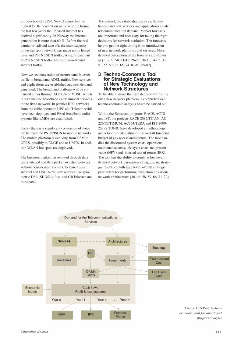
111Telektronikk 3/4.2003
introduction of ISDN. Now, Telenor has thehighest ISDN penetration in the world. Duringthe last few years the IP based Internet hasevolved significantly. In Norway the Internetpenetration is more than 60 %. Before the resi-dential broadband take off, the main capacityin the transport network was made up by leasedlines and PSTN/ISDN traffic. A significant partof PSTN/ISDN traffic has been narrowbandInternet traffic.
Now we see conversion of narrowband Internettraffic to broadband ADSL traffic. New servicesand applications are established and new demandgenerated. The broadband platform will be en-hanced either through ADSL2+ or VDSL, whichin turn include broadband entertainment servicesin the fixed network. In parallel HFC networksfrom the cable operators UPC and Telenor Avidihave been deployed and Fixed broadband radiosystems like LMDS are established.
Today there is a significant conversion of voicetraffic from the PSTN/ISDN to mobile networks.The mobile platform is evolving from GSM toGPRS, possibly to EDGE and to UMTS. In addi-tion WLAN hot spots are deployed.
The business market has evolved through dataline switched and data packet switched networkwithout considerable success, to leased lines,Internet and DSL. Now, new services like sym-metric DSL (SHDSL), fast- and GB Ethernet areintroduced.
The market, the established services, the en-hanced and new services and applications createtelecommunication demand. Market forecastsare important and necessary for taking the rightdecisions for network evolution. The forecastshelp to get the right timing from introductionof new network platforms and services. Moredetailed description of the forecasts are shownin [1, 3, 5, 7-8, 11-13, 26-27, 30-31, 34-35, 37,51, 55, 57, 63, 65, 74, 82-83, 85-87].
3 Techno-Economic Toolfor Strategic Evaluationsof New Technology andNetwork Structures
To be able to make the right decision for rollingout a new network platform, a comprehensivetechno-economic analysis has to be carried out.
Within the European programs RACE, ACTSand IST, the projects RACE 2087/TITAN, AC226/OPTIMUM, AC364/TERA and IST-2000-25172 TONIC have developed a methodologyand a tool for calculation of the overall financialbudget of any access architecture. The tool han-dles the discounted system costs, operations,maintenance costs, life cycle costs, net presentvalue (NPV) and internal rate of return (IRR).The tool has the ability to combine low level,detailed network parameters of significant strate-gic relevance with high level, overall strategicparameters for performing evaluation of variousnetwork architectures [40–46, 58–59, 66, 71–72].
Figure 1 TONIC techno-economic tool for investment
projects analysisNPV IRR
Investments
Services Architectures
Year Year Year Year. . .
PaybackPeriod
EconomicInputs
Revenues
OA&MCosts
Life CycleCost
First InstalledCost
Topology
ServicesServices Architectures
Year 0 Year m. . .
Demand for the TelecommunicationsServices
DB
Cash flows,Profit & loss accounts
Year 1 Year n
112 Telektronikk 3/4.2003
Figure 1 shows a techno-economic tool used indifferent international EU projects.
The figure shows that telecommunication de-mand is an input to the tool and to the techno-economic calculations. The TONIC tool iswidely used to analyse economic consequencesby implementing new network platforms. Impor-tant parts of the tool are:
• Service definitions• Subscription and traffic forecasts• Service tariff predictions• Revenue model• A topology model mapping geographic areas
with given penetrations into the tool• Network component cost data base including
more than 300 network components• Network component cost prediction model• Investment model• Operation and maintenance model• Model for economic calculations• Risk analysis model
The following steps are needed in the techno-economic evaluations of the network solutions:
The services to be provided must be specified.The market penetration of these services over thestudy period will be defined. The services haveassociated tariffs, i.e. the part of the tariff that isattributed to the network under study. From thecombination of yearly market penetration andyearly tariff information TONIC calculates therevenues for each year for the selected service set.
Next, the architecture scenarios to provide theselected service set must be defined. This needsnetwork design expertise and is mostly outsideof the framework of TONIC methodology. How-ever, TONIC includes several geometric models,which facilitate the network design by automati-cally calculating lengths for cables and ducting.These geometric models are optional parts of themethodology and TONIC can be used withoutthem. The result of an architecture scenario defi-nition is a so-called shopping list. This list indi-cates the volumes of all network cost elements(equipment, cables, cabinets, ducting, installa-tion etc.) for each year of the study period andthe location of these network components in dif-ferent flexibility points and link levels.
The costs of the network components are calcu-lated using an integrated cost database devel-oped within the TONIC project, containing datagathered from many European sources. Archi-tecture scenarios together with the cost databasegive investments for each year.
The OA&M costs are divided into differentcomponents like cost of repair parts includingcivil work and operations and administrationcosts. Typically the OA&M costs are beingdriven by services, say by number of customersand number of critical network elements.
Investment costs together with the OA&M costsgive the life-cycle cost for the selected architec-ture scenario. Finally, by combining service rev-enues, investments, operating costs and generaleconomic inputs (e.g. discount rate, tax rate)OPTIMUM, cash flows and other economic fac-tors (NPV, IRR, Payback period etc) are calcu-lated.
4 Strategic Evaluationsof New Technology andNetwork Structures
The possibility to introduce new services, en-hanced services, new applications, additionaltraffic growth and generation of additional rev-enue is important for network operators. Strate-gies for introduction of new technologies andnetwork platforms open the possibilities for gen-eration of additional revenue. Some examples ofintroduction of new technology during the last20 years are:
• Establishment of NMT• Deployment of optical fibre and fibre technol-
ogy in the network• Digitalisation of the PSTN• Introduction of ISDN• Establishment of GSM• Introduction of Internet• Establishment of ATM network• Establishment of IP networks• Establishment of SDH transmission technology• Introduction of ADSL
The next step is enhancement of the ADSL plat-form to ADSL2+ or VDSL and for the mobilenetwork UMTS, WLAN and 4G. Importantinput for making the right decisions of introduc-ing new technology has been demand forecastsfor new and enhanced services. The forecastsand tariff predictions give revenue forecasts,which are used together with techno-economicanalysis to support decisions of introduction ofnew technology.
The traffic forecasts are also fundamental fordimensioning the networks and establishingoptimal network structures.
Techno-economic evaluations of new networktechnology is analysed in [2, 4, 14–15, 18–25,28–29, 33, 36, 38–39, 48, 50, 52–54, 60, 68, 70,76, 81, 84, 88–89].
113Telektronikk 3/4.2003
5 Subscriber/AccessForecasting
Network planning of the access network dependsheavily on subscriber forecasts. Until recently,substantial investments in the local telephoneexchanges have been based on forecasts of thesubscriber growth in the local area. The sub-scriber forecasts indicated time for expansionof the telephone exchange. In addition the sub-scriber forecasts were used together with queu-ing models to estimate the busy hour traffic vol-ume in the exchange. When the data traffic waslimited, Erlang’s dimensioning rule was used fortraffic dimensioning taking into account the dis-tribution of residential and business customers.30 years ago the business customer traffic wasdominating and the busy hour was around lunch.Now, traffic from residential customers is domi-nating on the main part of the Norwegian ex-changes. During the last few years the busy hourhas been moved from after the main televisionnews programme to the 21.00–22.00 period,mainly because of the Internet traffic.
ISDN was introduced in the Norwegian market10 years ago. There have been significant substi-tution effects between ISDN and PSTN in thisperiod. The ISDN forecasts consist of: 2B+Dresidential, 2B+D business and 30B+D business.Also multiple ISDN line forecasts will be imple-mented.
The ISDN forecasts have been important for plan-ning and providing new network components.
Because of competition and substitution effectsbetween services, the penetration of PSTN andISDN have saturated the Norwegian network.Now, the new PSTN and ISDN forecasts reflecta smaller number of subscribers. There are twomain reasons for the decrease:
• Some residential customers substitute theirmain telephone subscriptions with mobilesubscriptions
• Some residential customers substitute theirPSTN/ISDN Internet connections with ADSL.
These forecasts are crucial for network planning.The forecasts show as a function of time thespare capacity in the network regarding trafficcapacity and number of connections.
The subscriber forecasts have been importantalso for restructuring the access network. Theforecasts are used for planning and establishingservice connection points in the access networkand for dimensioning the access lines and fibrerings between the service connection points.
Subscription forecasts have been developed for(narrowband) Internet, ATM, ADSL, SHDSL,SHDSL point-to-point, Fast Ethernet and GBEthernet and leased lines. The subscription fore-casts give valuable information for planning, di-mensioning and expanding the network structure.
However, it is important to take into account sig-nificant substitution effects between the services.The ISDN and PSTN forecasts are mutuallydependent. The ADSL forecasts influence sig-nificantly the narrowband Internet forecastsand ISDN and PSTN forecasts. Lost PSTN andISDN market shares for the incumbent increasethe leased line demand forecasts. Subscriptionforecasts for 2.5G and 3G increase the leasedlines forecasts. Increased ADSL subscriber fore-casts and demand for LLUB increase the leasedline forecasts because of expansion of the trafficcapacity between DSLAM and broadband accesspoint, and because of additional traffic in thetransport network. Subscriber demand forecastsfor SHDSL and SHDSL point-to-point andpoint-to-multipoint will lower the leased linesforecasts, since the new services are leased linessubstitutes with cheaper tariffs and a degradedservice quality.
To be able to control the dependencies, forecast-ing models for the different services are linkedtogether.
6 Traffic ForecastingAn important part of network planning is designof network structures. The PSTN/ISDN consistsof the access network including local exchanges,region networks including group exchanges andthe long distance network including long dis-tance exchanges and national exchanges. Tomaintain a high degree of reliability, indepen-dent routes are established between local ex-changes and group exchanges on the one handand between group exchanges and long distanceexchanges on the other hand. Between the longdistance exchanges there is a logical mesh net-work. However, even when there is a mesh net-work there is a simpler physical network takinginto account the logical mesh network abilities.The physical network is based on deployed fibrerings and SDH transmission equipment.
Network planning designs optimal structure ofthe network with the nodes (exchanges) and theroutes by minimising the costs for a given redun-dancy. Important factors are the exchange sites,the route length and the capacity on the routes.Specific network planning tools have also beendeveloped to minimise the investments. Differ-ent tools have been developed for the access net-work and for the transport network. The toolscan be applied for establishing new networkstructures or for expanding the network.
114 Telektronikk 3/4.2003
The traffic forecasts are important input fordesigning the network and for dimensioning theexchanges and capacity on the different routesand as input to the network planning tools.
The busy hour traffic forecasts quantify increases/decreases in the traffic. The dimensioning calcu-lations based on queuing theory add some extracapacity to control random variation in the traf-fic load during the busy hours. When the trafficon a route or in an exchange approaches thecapacity, an expansion will be carried out. Theexpansion of the capacity will be based on theforecasts for a given planning period.
The forecasting procedure described is used notonly for the PSTN/ISDN but for other networkslike PSDN, Frame relay/ATM, Digital CrossConnect, various IP networks, networks formobile operators and leased lines. There are dif-ferent possibilities for making traffic forecasts.One possibility is to measure the traffic and usethe traffic measurements as a historic databasefor the forecasts. One problem is rerouting of thetraffic based on new network structures orbecause of change of interconnection sites in thenetwork. Such changes affect the traffic mea-surements, which have to be adjusted before theforecasts can be developed. Another possibilityis to analyse the total traffic growth in the givennetwork and make the forecasts on the aggre-gated level.
A detailed description of the traffic forecastingprocedure for the transport network is describedin [1]. The traffic forecasting procedure for thetransport network is rather complex since thenetwork carries business and residential trafficfrom all the other networks.
7 Capacity ForecastsModels for making traffic forecasts during thebusy hour have been described. However, thecapacity needed to carry the traffic is higher.Additional capacity has to be dimensioned tak-ing into account stochastic variations around themean traffic in the busy hour. Usually Erlang’sblocking formula is applied for voice traffic,while Lindberger’s approximation is useful fordimensioning the data traffic capacity [90]. Thetraffic will probably be transported on SDH sys-tems where packet overhead is added. In addi-tion the systems’ average load factor is less thanthe maximum capacity. Finally there will in gen-eral be some extra dimensioning since the ex-pansion of the network is planned and deployedstepwise. A planning period is defined as thetime between two expansions. The duration ofthe planning period is found by taking intoaccount the repeating costs by performing theexpansion and the unused investment meansduring part of the period. The optimal planning
period is found by minimising the total costs.The estimation of additional capacity depends onthe planning process and the technical systemsand will vary from one incumbent to another.
8 Forecasting MethodologiesA variety of forecasting models are used for pre-dicting the evolution of the telecommunicationmarket. An important task is collection and anal-ysis of statistics – historical data. A lot of re-sources are used to maintain rather large cus-tomer based systems. An extraction of datafrom these systems is used to create subscriptionstatistics, which is a base for subscriber fore-casts. In addition specific measurement systemsare established to extract traffic measurementson specific points in the networks and also onthe aggregated level.
The forecasting models take into account histori-cal data. The most common models for accessforecasts are:
• Diffusion models• Regression models• Econometric models• ARIMA models• Kalman filter models• Smoothing models
The access forecasting models have to take intoaccount substitution effects between services aspointed out in chapter 5. Even the competitionbetween the incumbent and the other operatorsinfluences not only the access forecasts but alsothe BOT and leased lines forecasts. Telenor isusing a rather comprehensive composite modelwhere the substitution effects between PSTN,ISDN, Leased lines, ADSL, VDSL/ADSL2+,HFC, FTTH, FWA are included. Important fac-tors in the model are the predicted technologycoverage for the coming years, the predictedmarket shares etc.
The most common models for traffic forecastsare:
• Regression models• Econometric models• ARIMA models• Kalman filter models• Smoothing models
In addition specific forecasting procedures canbe used. The traffic is generated by sources andmoves in a network from source to a set of sinks.To dimension the network, it is important toknow the traffic behaviour from the edge routersor the local exchanges. The traffic streams aremapped in a traffic matrix. Each element in thematrix denotes the traffic between two ex-changes. Suppose the number of exchanges is
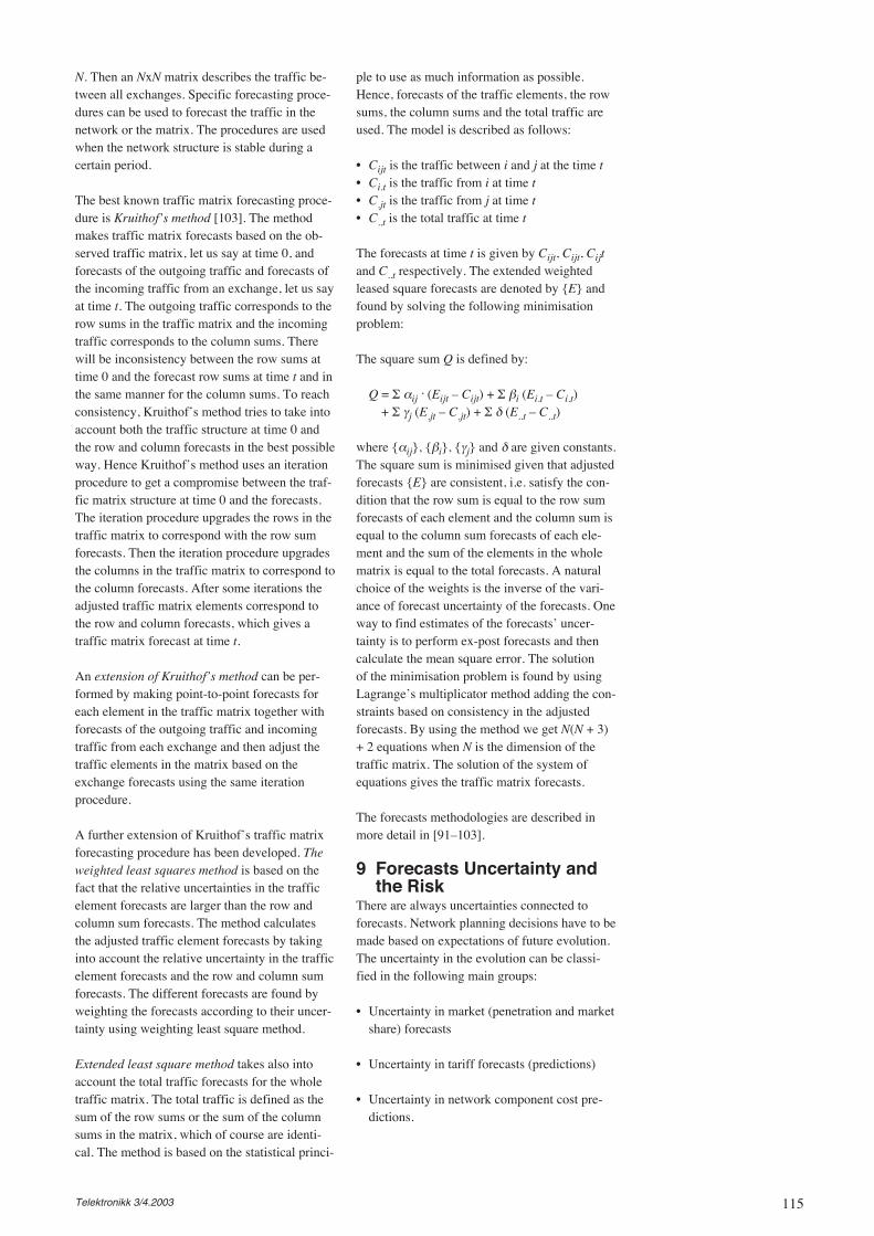
115Telektronikk 3/4.2003
N. Then an NxN matrix describes the traffic be-tween all exchanges. Specific forecasting proce-dures can be used to forecast the traffic in thenetwork or the matrix. The procedures are usedwhen the network structure is stable during acertain period.
The best known traffic matrix forecasting proce-dure is Kruithof’s method [103]. The methodmakes traffic matrix forecasts based on the ob-served traffic matrix, let us say at time 0, andforecasts of the outgoing traffic and forecasts ofthe incoming traffic from an exchange, let us sayat time t. The outgoing traffic corresponds to therow sums in the traffic matrix and the incomingtraffic corresponds to the column sums. Therewill be inconsistency between the row sums attime 0 and the forecast row sums at time t and inthe same manner for the column sums. To reachconsistency, Kruithof’s method tries to take intoaccount both the traffic structure at time 0 andthe row and column forecasts in the best possibleway. Hence Kruithof’s method uses an iterationprocedure to get a compromise between the traf-fic matrix structure at time 0 and the forecasts.The iteration procedure upgrades the rows in thetraffic matrix to correspond with the row sumforecasts. Then the iteration procedure upgradesthe columns in the traffic matrix to correspond tothe column forecasts. After some iterations theadjusted traffic matrix elements correspond tothe row and column forecasts, which gives atraffic matrix forecast at time t.
An extension of Kruithof’s method can be per-formed by making point-to-point forecasts foreach element in the traffic matrix together withforecasts of the outgoing traffic and incomingtraffic from each exchange and then adjust thetraffic elements in the matrix based on theexchange forecasts using the same iterationprocedure.
A further extension of Kruithof’s traffic matrixforecasting procedure has been developed. Theweighted least squares method is based on thefact that the relative uncertainties in the trafficelement forecasts are larger than the row andcolumn sum forecasts. The method calculatesthe adjusted traffic element forecasts by takinginto account the relative uncertainty in the trafficelement forecasts and the row and column sumforecasts. The different forecasts are found byweighting the forecasts according to their uncer-tainty using weighting least square method.
Extended least square method takes also intoaccount the total traffic forecasts for the wholetraffic matrix. The total traffic is defined as thesum of the row sums or the sum of the columnsums in the matrix, which of course are identi-cal. The method is based on the statistical princi-
ple to use as much information as possible.Hence, forecasts of the traffic elements, the rowsums, the column sums and the total traffic areused. The model is described as follows:
• Cijt is the traffic between i and j at the time t• Ci.t is the traffic from i at time t• C.jt is the traffic from j at time t• C..t is the total traffic at time t
The forecasts at time t is given by Cijt, Cijt, Cijtand C..t respectively. The extended weightedleased square forecasts are denoted by {E} andfound by solving the following minimisationproblem:
The square sum Q is defined by:
Q = Σ αij. (Eijt – Cijt) + Σ βi (Ei.t – Ci.t)
+ Σ γj (E.jt – C.jt) + Σ δ (E..t – C..t)
where {αij}, {βi}, {γj} and δ are given constants.The square sum is minimised given that adjustedforecasts {E} are consistent, i.e. satisfy the con-dition that the row sum is equal to the row sumforecasts of each element and the column sum isequal to the column sum forecasts of each ele-ment and the sum of the elements in the wholematrix is equal to the total forecasts. A naturalchoice of the weights is the inverse of the vari-ance of forecast uncertainty of the forecasts. Oneway to find estimates of the forecasts’ uncer-tainty is to perform ex-post forecasts and thencalculate the mean square error. The solutionof the minimisation problem is found by usingLagrange’s multiplicator method adding the con-straints based on consistency in the adjustedforecasts. By using the method we get N(N + 3)+ 2 equations when N is the dimension of thetraffic matrix. The solution of the system ofequations gives the traffic matrix forecasts.
The forecasts methodologies are described inmore detail in [91–103].
9 Forecasts Uncertainty andthe Risk
There are always uncertainties connected toforecasts. Network planning decisions have to bemade based on expectations of future evolution.The uncertainty in the evolution can be classi-fied in the following main groups:
• Uncertainty in market (penetration and marketshare) forecasts
• Uncertainty in tariff forecasts (predictions)
• Uncertainty in network component cost pre-dictions.
116 Telektronikk 3/4.2003
The effect of uncertainty in the predictions shouldbe quantified to examine the consequences. Thefirst step is to find the most critical variables inthe project. The next step is to perform calcula-tions based on variation in the critical variablesto identify the consequences.
One possibility is to apply sensitivity analysis.Another and more advanced method is to usethe risk analysis. The output in an economic riskanalysis is net present value (NPV), internal rateof return (IIR) and pay back period. One of theoutputs or all of them simultaneously can beused in risk analysis.
Instead of using the expected forecast, say attime t, a probability distribution of the forecastat time t has to be used. Similar probability dis-tributions have to be constructed for all criticalvariables. Usually truncated Normal distribu-tions or Beta distributions are used.
A Monte Carlo simulation with 1000 – 5000 tri-als is performed. In each trial, a random numberis picked from the predefined probability distri-butions; one for each of the critical variables.The simulation gives as output the cumulativedistribution of NPV, IIR and pay back periodand the ranking of the critical variables accord-
ing to their impact. This uncertainty ranking isbased on the percentage to the contribution tothe variance of the NPV or the rank correlationwith the NPV.
A commercial spreadsheet application CrystalBall has been integrated with the techno-eco-nomic tool. A graphical interface in Crystal Ballmakes it possible to specify the distributionfunctions directly from a palette type of menuinside the techno-economic model.
The risk analysis has been applied on a set ofdifferent cases studying strategies for rolling outnew network technology [6, 9–10, 16–17, 32,37, 47, 49, 56, 61–64, 67, 69, 73, 75, 77, 78–80].
10 ConclusionsThe paper documents that forecasts and forecastmethodology are important factors in the net-work planning process and strategy process forrolling out new technology platforms. Since theforecasts are uncertain, it is recommended to userisk analysis to evaluate the risk generated byforecasts and predictions of other critical vari-ables. For more detailed studies the papers inthe reference list should be studied.
Figure 2 Risk analysis
• Statistical Variation of the inputparameters
• Using Monte Carlo Simulation• Results: probability distribution,
risk profile of the business case• Extended basis for investment
decisions
Component Price
Service Penetration
Revenue per customer
0.68 0.74 0.80 0.86 0.92
1.09 1.54 2.00 2.46 2.91
0.55 0.78 1.00 1.23 1.45
kECU
Frequency Chart
.000
.007
.013
.020
.027
0
67.25
134.5
201.7
269
-3000 -1000 1000 3000 5000
10 000 Trials 52 Outliers
NPV

117Telektronikk 3/4.2003
References1 Stordahl, K. Traffic forecasting models for
the incumbent based on new drivers in themarket. Telektronikk, 99 (3/4), 122–127,2003 (this issue).
2 Elnegaard, N K, Olsen, B T, Stordahl, K.Broadband deployment in rural and noncompetitive areas: The European perspec-tive. In: Proc FITCE 2003, Berlin, Germany,September 1–4, 2003.
3 Stordahl, K, Kalhagen K O. Broadband fore-cast modelling. Evaluation of methodologyand results. International Symposium onForecasting 2003, Merida, Mexico, June16–19, 2003.
4 Welling, I et al. Techno-Economic Evalua-tion 3G & WLAN Business Case FeasibilityUnder Varying Conditions. In: Proc 10thInternational Conference on Telecommuni-cations, Tahiti, French Polynesia, February23 – March 1, 2003.
5 Stordahl, K, Kalhagen, K O. BroadbandAccess Forecasts for the European Market.Telektronikk, 98 (2/3), 21–32, 2002.
6 Elnegaard, N, Stordahl, K. Deciding on opti-mal timing of VDSL and ADSL roll-outs forincumbents. Telektronikk, 98 (2/3), 63–70,2002.
7 Kalhagen, K O, Elnegaard, N K. AssessingBroadband Investment Risk Trough OptionTheory. Telektronikk, 98 (2/3), 51–62, 2002.
8 Stordahl, K. Developing demand forecastsand tariff predictions for different telecomservices both for fixed and mobile based onresults from the IST TONIC project. IIRTelecoms Market Forecasting 2002, Prague,Czech Republic, October 7–10, 2002.
9 Kalhagen, K O, Elnegaard, N K. The Eco-nomics and Risks of 3rd Generation MobileService Deployment. Launching AppealingMobile Services, September 18–19, London,UK.
10 Elnegaard, N K. How to incorporate thevalue of flexibility in broadband access net-work rollout investment projects. 41st Euro-pean Telecommunications Congress (FITCE),Genova, Italy, September 4–7, 2002.
11 Stordahl, K, Kalhagen, K O, Olsen, B T.Broadband technology demand in Europe.2002 International Communications Fore-casting Conference, San Francisco, USA,June 25–28, 2002.
12 Hjelkrem, C, Stordahl, K, Bøe, J. Forecast-ing residential broadband demand with lim-ited information. A long term supply anddemand model. 2002 International Commu-nications Forecasting Conference, San Fran-cisco, USA, June 25–28, 2002.
13 Olsen, B T, Stordahl, K. Traffic forecastmodels for the transport network. In: ProcNetworks 2002, Munich, Germany, June23–27, 2002.
14 Monath, T et al. Economics of Ethernet ver-sus ATM-based access networks for broad-band IP services. In: Proc Networks 2002,Munich, Germany, June 23–27, 2002.
15 Varoutas D et al. Economic viability of 3GMobile Virtual Network Operators. In: Proc3G Wireless 2002, San Francisco, USA,May 28–31, 2002.
16 Kalhagen, K O, Elnegaard, N K. The Eco-nomics and Risks of 3rd Generation MobileService Deployment. In: Proc 3G 2002,Amsterdam, Netherlands, May 20–23, 2002.
17 Stordahl, K, Elnegaard, N K. Battle betweencable operator and incumbent: OptimalADSL/VDSL rollout for the incumbent. In:Proc. XIV International Symposium on Ser-vices in the Local access, ISSLS 2002, Seoul,Korea, April 14–18, 2002.
18 Olsen, B T, Kalhagen, K O, Stordahl, K.Provisioning of broadband services in non-competitive areas. In: Proc. XIV Interna-tional Symposium on Services in the Localaccess, ISSLS 2002, Seoul, Korea, April14–18, 2002.
19 Elnegaard, N K, Stordahl, K. Deciding onthe right timing of VDSL rollouts: A realoptions approach. In: Proc. XIV Interna-tional Symposium on Services in the Localaccess, ISSLS 2002, Seoul, Korea, April14–18, 2002.
20 Monath, T et al. Economics of Fixed AccessNetworks for broadband IP services (in Ger-man). 3. ITG-Fachtagung Netze und Anwen-dungen, Duisburg, Germany, February 28 –March 1, 2002.
21 Katsianis, D et al. The financial perspectiveof the mobile networks in Europe. IEEE Per-sonal Communications Magazine, 8 (6),58–64, 2001.

118 Telektronikk 3/4.2003
22 Ims, L A et al. Building a solid business planfor developing fibre in the access network.In: Proc. Optical Access Networks, London,UK, Oct 3–5, 2001.
23 Ims, L A et al. End-to-end-solutions for Tel-cos – is it a Broadcaster’s World? In: Proc.Interactive Convergence, London, UK, Sep3–5, 2001.
24 Ims, L A et al. From a large scale VDSLmarket trial towards commercial services –key issues. In: Proc. DSLCon Asia, HongKong, China, Aug 13–16, 2001.
25 Elnegaard, N K et al. From VDSL markettrials to commercial launch – The key issueson content, services, technical platform andthe business case. In: Proc. XDSL Summit,Geneva, Switzerland, July 11–13, 2001.
26 Hjelkrem, C. Forecasting with limited infor-mation: A study of the Norwegian ISDNaccess market. Journal of Business Fore-casting, 20 (3), 2001.
27 Stordahl, K, Elnegaard, N K, Olsen, B T.Broadband access rollout strategies in acompetitive environment. In: Proc. OpticalHybrid Access Network/Full Service AccessNetwork workshop, Yokohama, Japan, April3–5, 2001.
28 Ims, L A et al. Market driven deploymentof next generation networks – increasingthe service footprint by hybrid broadbandaccess. In: Proc. Hybrid Optical AccessNetwork 2001 (HOAN 2001), Yokohama,Japan, April 3–5, 2001.
29 Elnegaard, N K, Stordahl, K. Broadbandrollout strategies. In: Proc. 17th EuropeanNetwork Planning Workshop, Les Arcs,France, March 19–23, 2001.
30 Stordahl, K, Elnegaard, N K. Broadbandmarket evolution in Europe and the upgraderisks. 2000 International CommunicationsForecasting Conference, Seattle, USA,September 26–29, 2000.
31 Stordahl, K, Moe, M, Ims, L A. Broadbandmarket – The driver for network evolution.In: Proc. Networks 2000, Toronto, Canada,September 10–16, 2000.
32 Elnegaard, N K, Stordahl, K, Ims, L A. Therisks of DSL access network rollouts. In:Proc. Networks 2000, Toronto, Canada,September 10–16, 2000.
33 Stordahl, K et al. Optimal roll out strategiesfor XDSL broadband upgrades of the accessnetwork. In: Proc. International Telecommu-nication Society 2000, Buenos Aires,Argentina, July 2–5, 2000.
34 Stordahl, K, Ims, L A, Moe, M. Forecasts ofbroadband market evolution in Europe. In:Proc. International TelecommunicationSociety 2000, Buenos Aires, Argentina, July2–5, 2000.
35 Hjelkrem, C. Forecasting access demandwhen information is scarce : A case study ofthe Norwegian ISDN market. In: Proc. Inter-national Telecommunication Society 2000,Buenos Aires, Argentina, July 2–5, 2000.
36 Cerboni, A et al. Evaluation of demand fornext generation mobile services. In: Proc.International Telecommunication Society2000, Buenos Aires, Argentina, July 2–5,2000.
37 Stordahl, K et al. Broadband upgrading andthe risk of lost market shares Under Increas-ing Competition. In: Proc. ISSLS 2000,Stockholm, Sweden, June 19–23, 2000.
38 Elnegaard, N K, Stordahl, K, Ims, L A. Roll-Out Strategies for the Copper Access Net-work: Evolution towards a Full ServiceAccess Network. In: Proc. ISSLS 2000,Stockholm, Sweden, June 19–23, 2000.
39 Katsianis, D et al. The Economics of NextGeneration Mobile Systems. ISSLS 2000,Stockholm, Sweden, June 19–23, 2000.
40 Olsen, B T. Introduction to telecom invest-ments and techno-economics. SAS session.Techno-economics of multimedia servicesand networks, ICC 2000, New Orleans,USA, June 18–22, 2000.
41 Stordahl, K. Broadband market evolution –demand forecasting and tariffs. SAS session.Techno-economic methodologies and casestudies, ICC 2000, New Orleans, June18–22, 2000.
42 Ims, L A. Designing case studies. SAS ses-sion. Techno-economics of multimedia ser-vices and networks, ICC 2000, New Orleans,USA, June 18–22, 2000.
43 Olsen, B T. The TERA project – main objec-tives and results. SAS session. Techno-eco-nomics of multimedia services and networks.ICC 2000, New Orleans, USA, June 18–22,2000.

119Telektronikk 3/4.2003
44 Stordahl, K. Overview of risks in multimedianetworks. SAS session. Techno-economicmethodologies and case studies, ICC 2000,New Orleans, June 18–22, 2000.
45 Ims, L A. Case studies on broadband access:HFC, LMDS, VDSL, ADSL. SAS session.Techno-economics of multimedia servicesand networks, ICC 2000, New Orleans,USA, June 18–22, 2000.
46 Olsen, B T. The challenge of predicting costevolution. SAS session. Techno-economicsof multimedia services and networks, ICC2000, New Orleans, USA, June 18–22, 2000.
47 Stordahl, K. Case studies on broadbandaccess: Market risk analysis for fiber roll-out. SAS session. Techno-economics of mul-timedia services and networks, ICC 2000,New Orleans, USA, June 18–22, 2000.
48 Olsen, B T, Stordahl, K, Ims, L A. Evolutionof network architectures. In: Proc. 16thEuropean Network Planning Workshop,Les Arcs, France, March 20–24, 2000.
49 Stordahl, K et al. Overview of risks in Multi-media Broadband Upgrades. In: Proc.Globecom ’99, Rio de Janeiro, Brazil,December 5–10, 1999.
50 Ims, L A et al. The economics of broadbandinfrastructure upgrade investments in variousEuropean markets : The EURESCOM view.Telecom 99 Forum, Geneva, Switzerland,October 9–17, 1999.
51 Stordahl, K. Identifying the key risks in net-work development, taking into accountuncertainties in market forecasts and compe-tition. In: Proc. Future proof network plan-ning strategies, Vision in Business, Berlin,Germany, September 27–28, 1999.
52 Ims, L A. Introduction to broadband accessnetworks. Telektronikk, 95 (2/3), 2–22, 1999.
53 Ims, L A. Wireline broadband access net-works. Telektronikk, 95 (2/3), 73–87, 1999.
54 Ims, L A. Design of access network casestudies. Telektronikk, 95 (2/3), 251–253, 1999.
55 Stordahl K, Rand, L. Long term forecasts forbroadband demand. Telektronikk, 95 (2/3),34–44, 1999.
56 Stordahl, K, Ims, L A, Olsen, B T. Riskmethodology for evaluating broadbandaccess network architectures. Telektronikk,95 (2/3), 273–285, 1999.
57 Istad, S, Stordahl, K. Broadband demandsurvey in the residential and SOHO marketin Norway. Telektronikk, 95 (2/3), 45–49,1999.
58 Olsen, B T. OPTIMUM – a techno-eco-nomic tool. Telektronikk, 95 (2/3), 239–250,1999.
59 Tahkokorpi, M, Lähteenoja, M. Techno-Eco-nomic Guidelines for TelecommunicationNetworks and Services. Telektronikk, 95(2/3), 236–238, 1999.
60 Ims, L A et al. Towards broadband access inNorway – the view from Telenor. Telektron-ikk, 95 (2/3), 191–201, 1999.
61 Elnegaard, N K, Ims, L A, Stordahl, K.Techno-economic risk assessment of PNOaccess network evolutionary paths. Telek-tronikk, 95 (2/3), 286–290, 1999.
62 Stordahl, K et al. Risk methodology formultimedia projects assessments. In: Proc.ECMAST 1999, Madrid, Spain, May 26–28,1999.
63 Stordahl, K. Evaluation of key risks inbroadband network development taking intoaccount uncertainties in market forecasts andcompetition. In: Proc. Future Network Plan-ning Strategies, Vision in Business, London,March 2–4, 1999.
64 Elnegaard, N K, Stordahl, K. Technologychoice risk analysis and its impact on yourbusiness development and market position-ing. In: Proc. Future Proof Network Plan-ning Strategies, Vision in Business, London,UK, March 2–4, 1999.
65 Hjelkrem, C. Forecasting the demand forISDN accesses when the information isscarce : A case study from the Norwegianmarket. International Business Forecasting99, Las Vegas, USA, February 26, 1999.
66 Budry, L et al. The economics of broadbandservice introduction : Area specific invest-ments for broadband upgrade. In: Proc.TRIBAN, Bern, Switzerland, November17–19, 1998.
67 Stordahl, K et al. Broadband access networkcompetition – analysis of technology andmarket risks. In: Proc. Globecom ‘98, Syd-ney, November 8–12, 1998.

120 Telektronikk 3/4.2003
68 Ims, L A et al. Economics of broadbandaccess network upgrade strategies: TheEuropean perspective. In: Proc. Globecom’98 Access Networks Mini Conference,Sydney, November 8–12, 1998.
69 Stordahl, K et al. Evaluating broadbandstrategies in a competitive market using riskanalysis. In: Proc. Networks 98, Sorrento,October 18–23, 1998.
70 Ims, L A, Myhre, D, Olsen, B T. Investmentcosts of broadband capacity upgrade strate-gies in residential areas. In: Proc. Networks98, Sorrento, Italy, October 18–23, 1998.
71 Lähteenoja, M et al. Broadband access net-works: techno-economic methodology andtool application results. IEEE symposiumon planning and design of broadband Net-works, Montebello, Quebec, October 8–11,1998.
72 Ims, L A (ed). Broadband Access networks :Introduction Strategies and Techno-eco-nomic Evaluation. London, Chapman &Hall, 1998. (ISBN 0 412 82820 0)
73 Stordahl, K, Ims, L A, Olsen, B T. Riskanalysis of residential broadband upgradesbased on market evolution and competition.In: Proc. Supercom ICC ’98, Atlanta, June7–11, 1998.
74 Stordahl, K. Forecasting long term demandfor broadband services. In: Proc. Marketforecasts in the telecoms industry, Instituteof International Research (IIR), Hong Kong,May 25–27, 1998.
75 Olsen, B T et al. Multimedia business casesin a deregulated environment : Opportunitiesand risks. ISSLS 1998, Venice, March22–27, 1998.
76 Ims, L A et al. Key factors influencinginvestment strategies of broadband accessnetwork upgrades. In: Proc. ISSLS ‘98,Venice, Italy, March 22–27, 1998.
77 Stordahl, K. Evaluating broadband upgradestrategies in a competitive market using riskanalysis. Institute of International Research(IIR). In: Proc. Evaluating Broadband Ser-vice Strategies, London, UK, February18–20, 1998.
78 Ims, L A, Stordahl, K, Olsen, B T. Riskanalysis of residential broadband upgrade ina competitive environment. IEEE Communi-cation Magazine, June, 1997.
79 Ims, L A, Olsen, B T, Myhre, D. Economicsof residential broadband access networktechnologies and strategies. IEEE Networks,11 (1), 58–64, 1997.
80 Stordahl, K. Risk assessments of broadbandupgrade strategies. In: Proc. Broadbandstrategies – the battle for the customer, IBCconference, London, December 4–5, 1997.
81 Ims, L A et al. Evolution of technologies andarchitectures to a full services network. In:Proc. Broadband strategies – the battle forthe customer, IBC conference London,December 4–5, 1997.
82 Stordahl, K. Forecasting long term demandfor broadband services and their influenceon broadband evolution. Institute of Interna-tional Research (IIR). In: Proc. MarketForecasting in the Telecoms Industry,London, UK, December 1–4, 1997.
83 Stordahl, K, Ims, L A, Olsen, B T. Forecastsand risk analysis of PNO and Cable opera-tors by introducing broadband upgrades inthe access network. 1997 InternationalCommunication Forecasting Conference,San Francisco, June 24–27, 1997.
84 Ims, L A et al. Key factors influencing theoverall costs and project values of broadbandaccess network upgrades. NOC ‘97,Antwerp, Belgium, June 17–20, 1997.
85 Stordahl, K. Forecasting long term demandfor broadband services in the residentialmarket: Devising a method for developingforecasts for new services. Institute of Inter-national Research (IIR). In: Proc. MarketForecasting in the Telecoms Industry, Lon-don, UK, May 19–21, 1997.
86 Hjelkrem, C. Forecasting models for ISDNaccesses in the Norwegian market and theirinfluences on the investments strategies.Institute of International Research (IIR). In:Proc. Market Forecasting in the TelecomsIndustry, London, UK, May 19–21, 1997.
87 Stordahl, K. Techno-economic analysis,market forecasts and risk analysis of broad-band access network upgrading. In: Proc.13th European Network Planning Workshop,Les Arcs, France, March 9–15, 1997.
88 Olsen, B T. Access Network Evolution. In:Proc. 13th European Network PlanningWorkshop, Les Arcs, France, March 9–15,1997.

121Telektronikk 3/4.2003
89 Olsen, B T et al. Techno-economic evalua-tion of narrowband and broadband accessnetwork alternatives and evolution scenarioassessment. IEEE Journal of Selected Areasin Communications, 14 (8), 1996.
90 Lindberger, K. Analytical methods for thetraffical problems with statistical multiplex-ing in ATM network. In: Proc. 13th Interna-tional Teletraffic Congress, Copenhagen,June 19–26, 1991.
91 Stordahl, K. Methods for traffic matrix fore-casting. In: Proc. 12th International Tele-traffic Congress, Torino, Italy, June 1–8,1988.
92 Stordahl, K. Extended weighted minimumsquared method for forecasting traffic matri-ces. In: Proc. VII Nordic TeletrafficSeminar, Lund, Sweden, August 25–27,1987.
93 Stordahl, K. Forecasting models for networkplanning. In: Proc. VI Nordic TeletrafficSeminar, Copenhagen, Denmark, August28–30, 1986.
94 Stordahl, K, Damsleth, E. Traffic forecastingmethods for network planning. In: Proc. 6thInternational Conference on Forecastingand analysis for business in the informationage, Tokyo, Japan, August 1986.
95 ITU. Procedures for traffic matrix forecast-ing. Geneva, ITU, 1986. CCITT Com II 50-E.
96 Stordahl, K. Prognoser som grunnlag forplanlegging. (“Forecasts as a base for plan-ning”). Telektronikk, 82 (3), 1986.
97 Stordahl, K, Holden, L. Traffic forecastingmodels based on top down and bottom upprocedures. In: Proc. 11th InternationalTeletrafic Congress, Kyoto, Japan, Septem-ber 1985.
98 Stordahl, K. Routing algorithms based ontraffic forecast modelling. Time series analy-ses – Theory and practice. O D Anderson(ed.). Amsterdam, North Holland PublishingCompany, 1985.
99 Stordahl, K. Forecasting models for traffic inthe future broadband network. In: Proc. VNordic Teletraffic Seminar, Trondheim, Nor-way, June 5–7, 1984.
100 ITU. Forecasting of traffic. Geneva, ITU,1984. CCITT Red Book Rec E.506.
101Stordahl, K. Routing algorithms based ontraffic forecast modelling. Time series analy-ses – Theory and practice. Toronto, Canada,August 18–21, 1983.
102Stordahl, K. Centralized routing based onforecasts of the telephone traffic. In: Proc.10th International Teletraffic Congress,Montreal, Canada, June 1983.
103Kruithof, J. Telefoonverkeerrsrekening. DeIngenieur, 52 (8), 1937.
Telektronikk 3/4.2003
1 IntroductionThe circuit switched voice traffic has tradition-ally been a significant part of the traffic in thetransport network. However, during recent yearsLeased lines ordered by different operators andalso the Leased lines ordered from the businessmarket have expanded the transport networkcapacity. A new capacity wave has also started:the data traffic moving from narrowband tobroadband. The data traffic is increasing expo-nentially and will for some years be the dominat-ing traffic in the transport network. Importanttraffic drivers are broadband applications carriedby HFC, ADSL, VDSL, LMDS, UMTS andWLAN.
This paper analyses the traffic and capacity evo-lution of the transport network of an incumbentoperator having the possibility to integrate dif-ferent type of traffic into the network. A trafficvolume indicator is developed for traffic in-crease in the transport network. The access fore-cast modelling has been developed based onparts of the results from the projects ACT 384TERA and IST-2000-25172 project TONIC[1–16].
2 Market Segments
ServicesTraffic from the services is transported on differ-ent network platforms or on leased lines. Impor-tant services for the transport network are:PSTN/ISDN, Internet, Leased lines, PSDN(packet switched data network), Frame relay,ATM, IP Virtual private network (VPN),ADSL/SDSL, VDSL/LMDS, Fast Ethernet,Gigabit Ethernet, Lamda wavelength, Dynamicbandwidth allocation.
Market SegmentsAn incumbent operator leases transport capacityto other operators. In addition the incumbentoffers transport capacity to the residential andthe business market. The incumbent operatoroffers transport capacity either via own serviceprovider or as wholesale. A segmentation of themarket will be:
Residential market: PSTN, ISDN, Internet,ADSL, VDSL, LMDS, HFC.
Business market: PSTN, ISDN, IP VPN, Inter-net, PSDN, Frame Relay, ATM, ADSL, SDSL,VDSL, LMDS, Leased lines, Fast Ethernet,
Gigabit Ethernet, Lamda wavelength, Dynamicbandwidth allocation.
Operators: ADSL, SDSL, VDSL, LMDS,Leased lines, Fast Ethernet, Gigabit Ethernet IP-VPN, Lamda wavelength, Dynamic bandwidthallocation. (mobile operators, ISPs, other opera-tors).
Network PlatformsRelevant network platforms are: PSTN/ISDN,PSDN, Frame Relay/ATM, Digital Cross Con-nect, Various IP Networks including IP net-works for mobile operators, Leased lines.PSTN/ISDN is a circuit switched network.Leased lines have no concentration effect at all,while the other network platforms also havepacket switched concentration.
3 Traffic From the ResidentialMarket
The residential market generates different typesof traffic: Voice traffic, Dialled Internet traffic,ADSL traffic, VDSL/LMDS traffic.
The voice traffic has nearly reached saturation.During the next years, the circuit switched voicetraffic will be rather stable before parts of thecircuit switched voice traffic are substituted byIP voice. The dialled Internet traffic will reachmaximum within a few years. Then the dialledInternet traffic will continuously be substitutedby broadband traffic. A battle has already startedbetween broadband operators to capture partsof the broadband market.
Broadband access forecasts have been developedin the IST-2000-25172 project TONIC. Figure 1shows the market share evolution of ADSL,VDSL, FWA (Fixed wireless broadband access)and HFC/cable modem for West European coun-tries.
Figure 2 shows total broadband penetration. Thetotal broadband penetration forecasts are ad-justed compared to the forecasts developed inthe TONIC projects. A combination of the fig-ures gives the broadband penetration for eachtechnology.
Now, the question is which traffic is carried inthe incumbent’s transport network. Usually thecable TV/HFC traffic is carried outside the trans-port network, while a part (market share) of the
Traffic Forecasting Models for the Incum-bent Based on New Drivers in the MarketK J E L L S T O R D A H L
Kjell Stordahl (58) received hisM.S. in statistics from Oslo Uni-versity in 1972. He worked withTelenor R&D for 15 years andwith Telenor Networks for 15years, mainly as manager ofPlanning Department RegionOslo and then Market analysis.Since 1992 he has participatedin various techno-economic EUprojects (TITAN, OPTIMUM,TERA, TONIC) analysing rolloutof different broadband technolo-gies. Kjell Stordahl has beenresponsible for working pack-ages on broadband demand,forecasting and risk analysis inthese projects. He has pub-lished more than 140 papers ininternational journals and con-ferences.
122
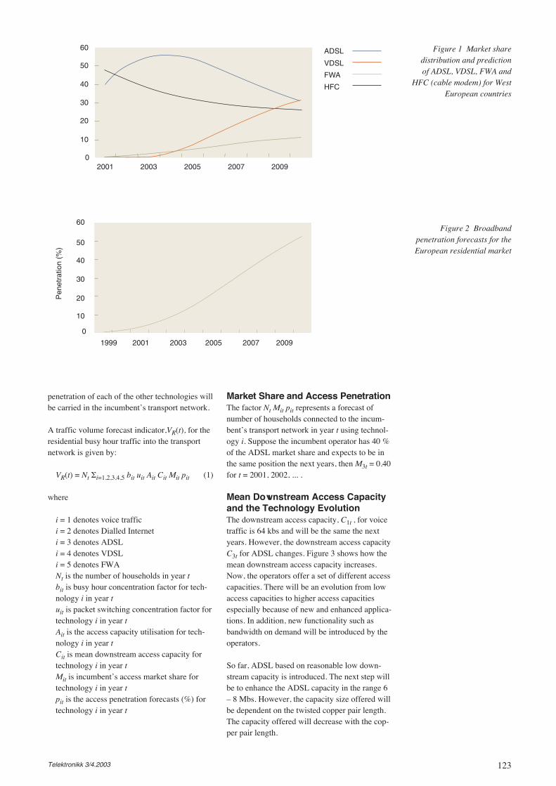
123Telektronikk 3/4.2003
penetration of each of the other technologies willbe carried in the incumbent’s transport network.
A traffic volume forecast indicator,VR(t), for theresidential busy hour traffic into the transportnetwork is given by:
VR(t) = Nt Σi=1,2,3,4,5 bit uit Ait Cit Mit pit (1)
where
i = 1 denotes voice traffici = 2 denotes Dialled Interneti = 3 denotes ADSLi = 4 denotes VDSLi = 5 denotes FWANt is the number of households in year tbit is busy hour concentration factor for tech-nology i in year tuit is packet switching concentration factor fortechnology i in year tAit is the access capacity utilisation for tech-nology i in year tCit is mean downstream access capacity fortechnology i in year tMit is incumbent’s access market share fortechnology i in year tpit is the access penetration forecasts (%) fortechnology i in year t
Market Share and Access PenetrationThe factor Nt Mit pit represents a forecast ofnumber of households connected to the incum-bent’s transport network in year t using technol-ogy i. Suppose the incumbent operator has 40 %of the ADSL market share and expects to be inthe same position the next years, then M3t = 0.40for t = 2001, 2002, ... .
Mean Downstream Access Capacityand the Technology EvolutionThe downstream access capacity, C1t , for voicetraffic is 64 kbs and will be the same the nextyears. However, the downstream access capacityC3t for ADSL changes. Figure 3 shows how themean downstream access capacity increases.Now, the operators offer a set of different accesscapacities. There will be an evolution from lowaccess capacities to higher access capacitiesespecially because of new and enhanced applica-tions. In addition, new functionality such asbandwidth on demand will be introduced by theoperators.
So far, ADSL based on reasonable low down-stream capacity is introduced. The next step willbe to enhance the ADSL capacity in the range 6– 8 Mbs. However, the capacity size offered willbe dependent on the twisted copper pair length.The capacity offered will decrease with the cop-per pair length.
Figure 2 Broadbandpenetration forecasts for theEuropean residential market
Figure 1 Market sharedistribution and predictionof ADSL, VDSL, FWA and
HFC (cable modem) for WestEuropean countries
0
10
20
30
40
50
60
2001 2003 2005 2007 2009
ADSL
VDSL
FWA
HFC
0
10
20
30
40
50
60
1999 2001 2003 2005 2007 2009
Pen
etra
tion
(%)
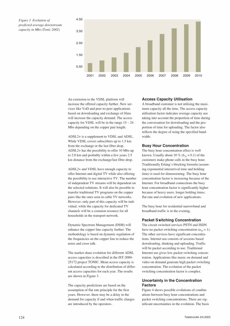
124 Telektronikk 3/4.2003
An extension to the VDSL platform willincrease the offered capacity further. New ser-vices like VoD and peer-to-peer applicationsbased on downloading and exchange of filmswill increase the capacity demand. The accesscapacity for VDSL will be in the range 15 – 24Mbs depending on the copper pair length.
ADSL2+ is a supplement to VDSL and ADSL.While VDSL covers subscribers up to 1.5 kmfrom the exchange or the last fibre drop,ADSL2+ has the possibility to offer 10 Mbs upto 2.0 km and probably within a few years 2.5km distance from the exchange/last fibre drop.
ADSL2+ and VDSL have enough capacity tooffer Internet and digital TV while also offeringthe possibility to use interactive TV. The numberof independent TV streams will be dependent onthe selected solutions. It will also be possible totransfer traditional TV programs on the copperpairs like the ones seen in cable TV networks.However, only part of this capacity will be indi-vidual, while the capacity for dedicated TVchannels will be a common resource for allhouseholds in the transport network.
Dynamic Spectrum Management (DSM) willenhance the copper line capacity further. Themethodology is based on dynamic regulation ofthe frequencies on the copper line to reduce thenoise and cross talk.
The market share evolution for different ADSLaccess capacities is described in the IST-2000-25172 project TONIC. Mean access capacity iscalculated according to the distribution of differ-ent access capacities for each year. The resultsare shown in Figure 3.
The capacity predictions are based on theassumption of flat rate principle for the firstyears. However, there may be a delay in thedemand for capacity if and when traffic chargesare introduced by the operators.
Access Capacity UtilisationA broadband customer is not utilising the maxi-mum capacity all the time. The access capacityutilisation factor indicates average capacity usetaking into account the proportion of time duringthe conversation for downloading and the pro-portion of time for uploading. The factor alsoreflects the degree of using the specified band-width.
Busy Hour ConcentrationThe busy hour concentration effect is wellknown. Usually about 10 % (b1t = 0.1) of thecustomers make phone calls in the busy hour.Traditionally Erlang’s blocking formula (assum-ing exponential interarrival time and holdingtime) is used for dimensioning. The busy hourconcentration factor is increasing because of theInternet. For broadband connections the busyhour concentration factor is significantly higherbecause of heavy users, longer holding times,flat rate and evolution of new applications.
The busy hour for residential narrowband andbroadband traffic is in the evening.
Packet Switching ConcentrationThe circuit switched services PSTN and ISDNhave no packet switching concentration (u1t = 1).The other services have significant concentra-tions. Internet use consists of sessions baseddownloading, thinking and uploading. Trafficwill be packet according to use. TraditionalInternet use gives low packet switching concen-tration. Applications like music on demand andvideo on demand generate high packet switchingconcentration. The evolution of the packetswitching concentration factor is complex.
Uncertainty in the ConcentrationFactorsFigure 4 shows possible evolutions of combin-ations between busy hour concentrations andpacket switching concentrations. There are sig-nificant uncertainties in the evolution. The basis
Figure 3 Evolution ofpredicted average downstreamcapacity in Mbs (Tonic 2002)
0.50
1.50
2.50
3.50
4.50
2001 2002 2003 2004 2005 2006 2007 2008 2009 2010
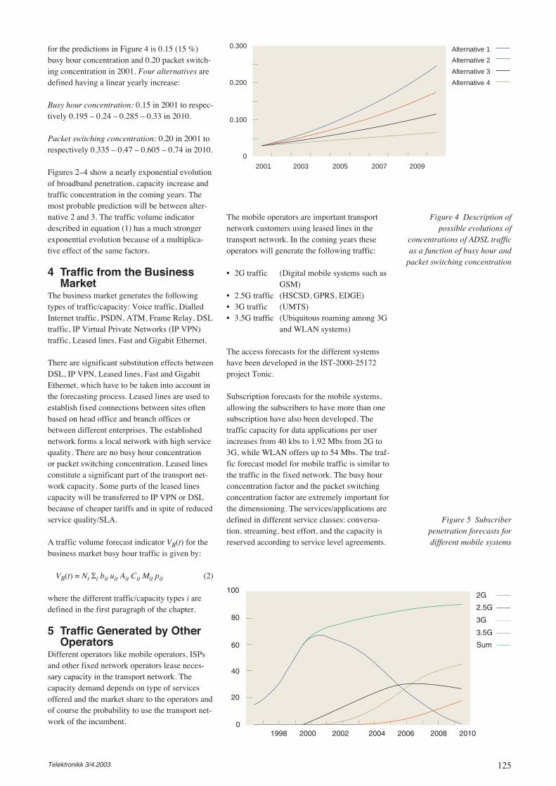
125Telektronikk 3/4.2003
for the predictions in Figure 4 is 0.15 (15 %)busy hour concentration and 0.20 packet switch-ing concentration in 2001. Four alternatives aredefined having a linear yearly increase:
Busy hour concentration: 0.15 in 2001 to respec-tively 0.195 – 0.24 – 0.285 – 0.33 in 2010.
Packet switching concentration: 0.20 in 2001 torespectively 0.335 – 0.47 – 0.605 – 0.74 in 2010.
Figures 2–4 show a nearly exponential evolutionof broadband penetration, capacity increase andtraffic concentration in the coming years. Themost probable prediction will be between alter-native 2 and 3. The traffic volume indicatordescribed in equation (1) has a much strongerexponential evolution because of a multiplica-tive effect of the same factors.
4 Traffic from the BusinessMarket
The business market generates the followingtypes of traffic/capacity: Voice traffic, DialledInternet traffic, PSDN, ATM, Frame Relay, DSLtraffic, IP Virtual Private Networks (IP VPN)traffic, Leased lines, Fast and Gigabit Ethernet.
There are significant substitution effects betweenDSL, IP VPN, Leased lines, Fast and GigabitEthernet, which have to be taken into account inthe forecasting process. Leased lines are used toestablish fixed connections between sites oftenbased on head office and branch offices orbetween different enterprises. The establishednetwork forms a local network with high servicequality. There are no busy hour concentrationor packet switching concentration. Leased linesconstitute a significant part of the transport net-work capacity. Some parts of the leased linescapacity will be transferred to IP VPN or DSLbecause of cheaper tariffs and in spite of reducedservice quality/SLA.
A traffic volume forecast indicator VB(t) for thebusiness market busy hour traffic is given by:
VB(t) = Nt Σi bit uit Ait Cit Mit pit (2)
where the different traffic/capacity types i aredefined in the first paragraph of the chapter.
5 Traffic Generated by OtherOperators
Different operators like mobile operators, ISPsand other fixed network operators lease neces-sary capacity in the transport network. Thecapacity demand depends on type of servicesoffered and the market share to the operators andof course the probability to use the transport net-work of the incumbent.
The mobile operators are important transportnetwork customers using leased lines in thetransport network. In the coming years theseoperators will generate the following traffic:
• 2G traffic (Digital mobile systems such asGSM)
• 2.5G traffic (HSCSD, GPRS, EDGE)• 3G traffic (UMTS)• 3.5G traffic (Ubiquitous roaming among 3G
and WLAN systems)
The access forecasts for the different systemshave been developed in the IST-2000-25172project Tonic.
Subscription forecasts for the mobile systems,allowing the subscribers to have more than onesubscription have also been developed. Thetraffic capacity for data applications per userincreases from 40 kbs to 1.92 Mbs from 2G to3G, while WLAN offers up to 54 Mbs. The traf-fic forecast model for mobile traffic is similar tothe traffic in the fixed network. The busy hourconcentration factor and the packet switchingconcentration factor are extremely important forthe dimensioning. The services/applications aredefined in different service classes: conversa-tion, streaming, best effort, and the capacity isreserved according to service level agreements.
Figure 4 Description ofpossible evolutions of
concentrations of ADSL trafficas a function of busy hour and
packet switching concentration
Figure 5 Subscriberpenetration forecasts fordifferent mobile systems
0
0.100
0.200
0.300
2001 2003 2005 2007 2009
Alternative 1
Alternative 2
Alternative 3
Alternative 4
0
20
40
60
80
1002G
2.5G
3G
3.5G
Sum
2010200820062004200220001998

126 Telektronikk 3/4.2003
The traffic forecasting model VM(t) for mobileoperators is given by:
VM(t) = Nt Σi bit uit Ait Cit Mit pit (3)
Here Nt is number of persons, not number ofhouseholds. Mit denotes the market share to theoperator and i = 1, 2, 3, 4 the system generations2G, 2.5G, 3G and 3.5G. The penetration fore-casts pit are shown in Figure 5. The capacity Cit
is a mean capacity. A 3.5G subscriber has thepossibility to use a data rate up to 144 kbs usingUMTS but a significantly higher capacity inWLAN hot spot. The number of hot spots avail-able and the proportion of time the subscriberuses WLAN compared with UMTS give themean capacity C4t . The factor Ait indicates thereal utilisation of the capacity.
Let VO(t) be the busy hour traffic forecasts forthe other operators, then the total of busy hourtraffic forecasts V(t) is given by:
V(t) = VR(t) + VB(t) + VM(t) + VO(t) (4)
There are definitely possibilities to reduce V(t)since the business traffic has busy hour before/after lunch, while the residential traffic has busyhour in the evening. Since the operators useleased lines, day and night capacity is equal. LetVBL(t) be the leased line capacity and VBP(t) bethe packet switched traffic in the business mar-ket. Then VB(t) = VBL(t) + VBP(t). The residentialbroadband traffic is larger than the packetswitched business traffic in the busy hour. Sup-pose that ∆ = 0.2 (20 %) of the packet switchedbusiness busy hour traffic is transferred duringthe residential busy hour the adjusted busy hourtraffic forecast V * (t) is:
V * (t) = VR(t) + ∆VBP(t) + VBL(t) + VM(t) + VO(t) (5)
6 Capacity ForecastsModels for making traffic forecasts during busyhour have been described. However, the capacityneeded to carry the traffic is higher. Additionalcapacity has to be dimensioned taking intoaccount stochastic variations around the meantraffic in the busy hour. Usually Erlang’s block-ing formula is applied for voice traffic, whileLindberger’s approximation is useful for dimen-sioning the data traffic capacity [12]. The trafficwill probably be transported on SDH systemswhere packet overhead is added. In addition thesystem’s load average factor is less than the max-imum capacity, and finally there will in generalbe some extra dimensioning since the expansionof the network is planned and deployed stepwise.The estimation of additional capacity depends onthe planning process and the technical systemsand will vary from one incumbent to another.
7 ConclusionsA traffic volume indicator has been developed toestimate busy hour traffic increase in the trans-port network. The indicator estimates the trafficentering the transport network. The traffic vol-ume indicator does not include redundancy andprotection capacity in the core network. Telenoruses the traffic volume indicator forecasts asinput to the transport network planning process –evaluation of new network structures, expansionof the network and introduction of new corenetwork technology.
The indicator depends on the application evolu-tion and also the tariff regime for broadbandservices. So far, most countries use a flat ratefor broadband traffic. However, specific applica-tions will overload the transport network heavilyif no actions are performed. There exist no in-citements to control the size of the traffic in thetransport network. A probable solution will beto introduce a tariff on high capacity traffic andon bandwidth on demand and specific applica-tions. The traffic forecasts used assume that anew tariff regime for broadband services willbe implemented within the next two years.
References1 Stordahl, K, Kalhagen, K O. Broadband
Access Forecasts for the European Market.Telektronikk, 98 (2/3), 21–32, 2002.
2 Elnegaard, N, Stordahl, K. Deciding on opti-mal timing of VDSL and ADSL roll-outs forincumbents. Telektronikk, 98 (2/3), 63–70,2002.
3 Stordahl, K, Kalhagen, K O, Olsen, B T.Broadband technology demand in Europe.ICFC 2002, San Francisco, USA, June25–28, 2002.
4 Stordahl, K, Elnegaard, N K. Battle betweencable operator and incumbent : OptimalADSL/VDSL rollout for the incumbent. In:Proc. XIV International Symposium on Ser-vices in the Local Access – ISSLS 2002,Seoul, Korea, April 14–18, 2002.
5 Monath, T et al. Economics of Ethernetbased Access Networks for broadband IPServices. Proc. ISSLS 2002, Seoul, Korea,April 14–18, 2002.
6 Stordahl, K, Elnegaard, N K. Risk analysisof broadband access rollout strategies in acompetitive environment. In: Proc. OpticalHybrid Access Network/Full Service AccessNetwork workshop, Yokohama, Japan, April4–6, 2001.

127Telektronikk 3/4.2003
7 Stordahl, K, Elnegaard, N K. Broadbandmarket evolution in Europe and the upgraderisks. ICFC, Seattle, September 26–29,2000.
8 Stordahl, K et al. Broadband market, thedriver for network evolution. In: Proc. Net-works 2000, Toronto, Canada, September10–15, 2000.
9 Elnegaard, N K, Ims, L A, Stordahl, K. Therisks of DSL access network rollouts. In:Proc. Networks 2000, Toronto, Canada,September 10–15, 2000.
10 Stordahl, K, Ims, L A, Moe, M. Forecasts ofbroadband market evolution in Europe. In:Proc. ITS 2000, Buenos Aires, Argentina,July 2–5, 2000.
11 Stordahl, K. Broadband market evolution –demand forecasting and tariffs. ICC 2000,SAS session. Techno-economics of multi-media services and networks. New Orleans,USA, June 18–22, 2000.
12 Stordahl, K et al. Broadband upgrading andthe risk of lost market share under increasingcompetition. In: Proc. ISSLS 2000, Stock-holm, Sweden, June 19–23, 2000.
13 Elnegaard, N K, Ims, L A, Stordahl, K. Roll-out strategies for the copper access network– evolution towards a full service access net-work. In: Proc. ISSLS 2000, Stockholm,Sweden, June 19–23, 2000.
14 Stordahl, K et al. Overview of risks in Multi-media Broadband Upgrades. In: Proc.Globecom ’99, Rio de Janeiro, Brazil, Dec5–10, 1999.
15 Stordahl, K et al. Evaluating broadbandstrategies in a competitive market using riskanalysis. In: Proc. Networks 98, Sorrento,Italy, Oct 18–23, 1998.
16 Ims, L A (ed.). Broadband Access Networks– Introduction strategies and techno-eco-nomic analysis. Chapman-Hall, 1998.
17 Lindberger, K. Dimensioning and designmethods for integrated ATM networks. In:Proc. 14th ITC, Antibes, France, June, 1994.
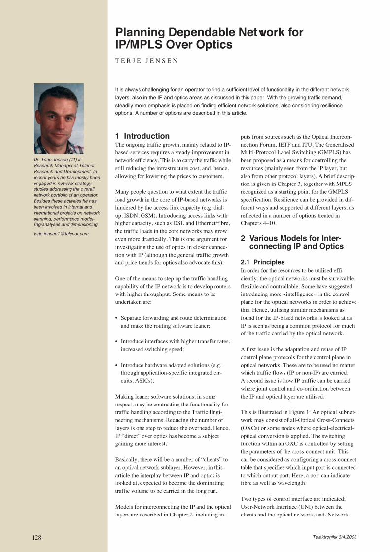
Telektronikk 3/4.2003
1 IntroductionThe ongoing traffic growth, mainly related to IP-based services requires a steady improvement innetwork efficiency. This is to carry the traffic whilestill reducing the infrastructure cost, and, hence,allowing for lowering the prices to customers.
Many people question to what extent the trafficload growth in the core of IP-based networks ishindered by the access link capacity (e.g. dial-up, ISDN, GSM). Introducing access links withhigher capacity, such as DSL and Ethernet/fibre,the traffic loads in the core networks may groweven more drastically. This is one argument forinvestigating the use of optics in closer connec-tion with IP (although the general traffic growthand price trends for optics also advocate this).
One of the means to step up the traffic handlingcapability of the IP network is to develop routerswith higher throughput. Some means to beundertaken are:
• Separate forwarding and route determinationand make the routing software leaner;
• Introduce interfaces with higher transfer rates,increased switching speed;
• Introduce hardware adapted solutions (e.g.through application-specific integrated cir-cuits, ASICs).
Making leaner software solutions, in somerespect, may be contrasting the functionality fortraffic handling according to the Traffic Engi-neering mechanisms. Reducing the number oflayers is one step to reduce the overhead. Hence,IP “direct” over optics has become a subjectgaining more interest.
Basically, there will be a number of “clients” toan optical network sublayer. However, in thisarticle the interplay between IP and optics islooked at, expected to become the dominatingtraffic volume to be carried in the long run.
Models for interconnecting the IP and the opticallayers are described in Chapter 2, including in-
puts from sources such as the Optical Intercon-nection Forum, IETF and ITU. The GeneralisedMulti-Protocol Label Switching (GMPLS) hasbeen proposed as a means for controlling theresources (mainly seen from the IP layer, butalso from other protocol layers). A brief descrip-tion is given in Chapter 3, together with MPLSrecognized as a starting point for the GMPLSspecification. Resilience can be provided in dif-ferent ways and supported at different layers, asreflected in a number of options treated inChapters 4–10.
2 Various Models for Inter-connecting IP and Optics
2.1 PrinciplesIn order for the resources to be utilised effi-ciently, the optical networks must be survivable,flexible and controllable. Some have suggestedintroducing more «intelligence» in the controlplane for the optical networks in order to achievethis. Hence, utilising similar mechanisms asfound for the IP-based networks is looked at asIP is seen as being a common protocol for muchof the traffic carried by the optical network.
A first issue is the adaptation and reuse of IPcontrol plane protocols for the control plane inoptical networks. These are to be used no matterwhich traffic flows (IP or non-IP) are carried.A second issue is how IP traffic can be carriedwhere joint control and co-ordination betweenthe IP and optical layer are utilised.
This is illustrated in Figure 1: An optical subnet-work may consist of all-Optical Cross-Connects(OXCs) or some nodes where optical-electrical-optical conversion is applied. The switchingfunction within an OXC is controlled by settingthe parameters of the cross-connect unit. Thiscan be considered as configuring a cross-connecttable that specifies which input port is connectedto which output port. Here, a port can indicatefibre as well as wavelength.
Two types of control interface are indicated;User-Network Interface (UNI) between theclients and the optical network, and, Network-
Planning Dependable Network forIP/MPLS Over OpticsT E R J E J E N S E N
It is always challenging for an operator to find a sufficient level of functionality in the different network
layers, also in the IP and optics areas as discussed in this paper. With the growing traffic demand,
steadily more emphasis is placed on finding efficient network solutions, also considering resilience
options. A number of options are described in this article.
Dr. Terje Jensen (41) isResearch Manager at TelenorResearch and Development. Inrecent years he has mostly beenengaged in network strategystudies addressing the overallnetwork portfolio of an operator.Besides these activities he hasbeen involved in internal andinternational projects on networkplanning, performance model-ling/analyses and dimensioning.
128
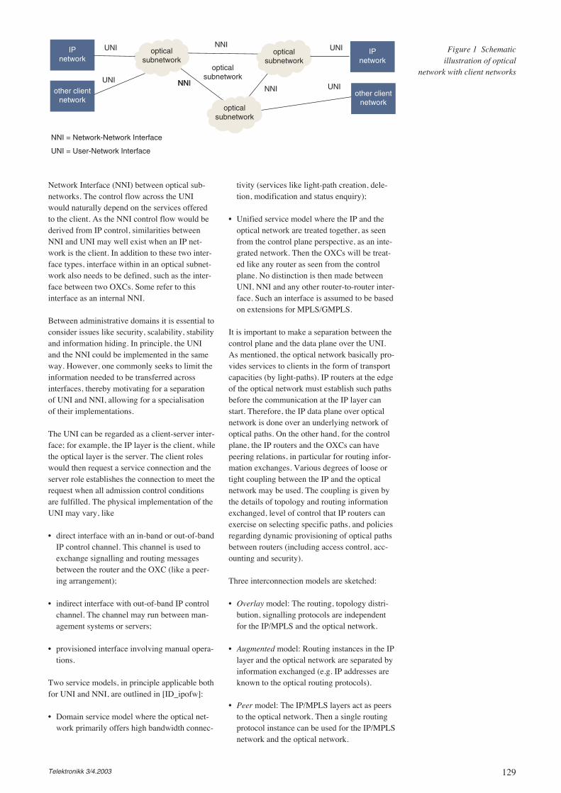
129Telektronikk 3/4.2003
Network Interface (NNI) between optical sub-networks. The control flow across the UNIwould naturally depend on the services offeredto the client. As the NNI control flow would bederived from IP control, similarities betweenNNI and UNI may well exist when an IP net-work is the client. In addition to these two inter-face types, interface within in an optical subnet-work also needs to be defined, such as the inter-face between two OXCs. Some refer to thisinterface as an internal NNI.
Between administrative domains it is essential toconsider issues like security, scalability, stabilityand information hiding. In principle, the UNIand the NNI could be implemented in the sameway. However, one commonly seeks to limit theinformation needed to be transferred acrossinterfaces, thereby motivating for a separationof UNI and NNI, allowing for a specialisationof their implementations.
The UNI can be regarded as a client-server inter-face; for example, the IP layer is the client, whilethe optical layer is the server. The client roleswould then request a service connection and theserver role establishes the connection to meet therequest when all admission control conditionsare fulfilled. The physical implementation of theUNI may vary, like
• direct interface with an in-band or out-of-bandIP control channel. This channel is used toexchange signalling and routing messagesbetween the router and the OXC (like a peer-ing arrangement);
• indirect interface with out-of-band IP controlchannel. The channel may run between man-agement systems or servers;
• provisioned interface involving manual opera-tions.
Two service models, in principle applicable bothfor UNI and NNI, are outlined in [ID_ipofw]:
• Domain service model where the optical net-work primarily offers high bandwidth connec-
tivity (services like light-path creation, dele-tion, modification and status enquiry);
• Unified service model where the IP and theoptical network are treated together, as seenfrom the control plane perspective, as an inte-grated network. Then the OXCs will be treat-ed like any router as seen from the controlplane. No distinction is then made betweenUNI, NNI and any other router-to-router inter-face. Such an interface is assumed to be basedon extensions for MPLS/GMPLS.
It is important to make a separation between thecontrol plane and the data plane over the UNI.As mentioned, the optical network basically pro-vides services to clients in the form of transportcapacities (by light-paths). IP routers at the edgeof the optical network must establish such pathsbefore the communication at the IP layer canstart. Therefore, the IP data plane over opticalnetwork is done over an underlying network ofoptical paths. On the other hand, for the controlplane, the IP routers and the OXCs can havepeering relations, in particular for routing infor-mation exchanges. Various degrees of loose ortight coupling between the IP and the opticalnetwork may be used. The coupling is given bythe details of topology and routing informationexchanged, level of control that IP routers canexercise on selecting specific paths, and policiesregarding dynamic provisioning of optical pathsbetween routers (including access control, acc-ounting and security).
Three interconnection models are sketched:
• Overlay model: The routing, topology distri-bution, signalling protocols are independentfor the IP/MPLS and the optical network.
• Augmented model: Routing instances in the IPlayer and the optical network are separated byinformation exchanged (e.g. IP addresses areknown to the optical routing protocols).
• Peer model: The IP/MPLS layers act as peersto the optical network. Then a single routingprotocol instance can be used for the IP/MPLSnetwork and the optical network.
Figure 1 Schematicillustration of optical
network with client networksUNI
UNIIPnetwork
other clientnetwork
opticalsubnetwork
opticalsubnetwork
opticalsubnetwork
opticalsubnetwork
IPnetwork
other clientnetwork
UNI
UNI
NNINNI
NNI
NNI = Network-Network Interface
UNI = User-Network Interface
NNI
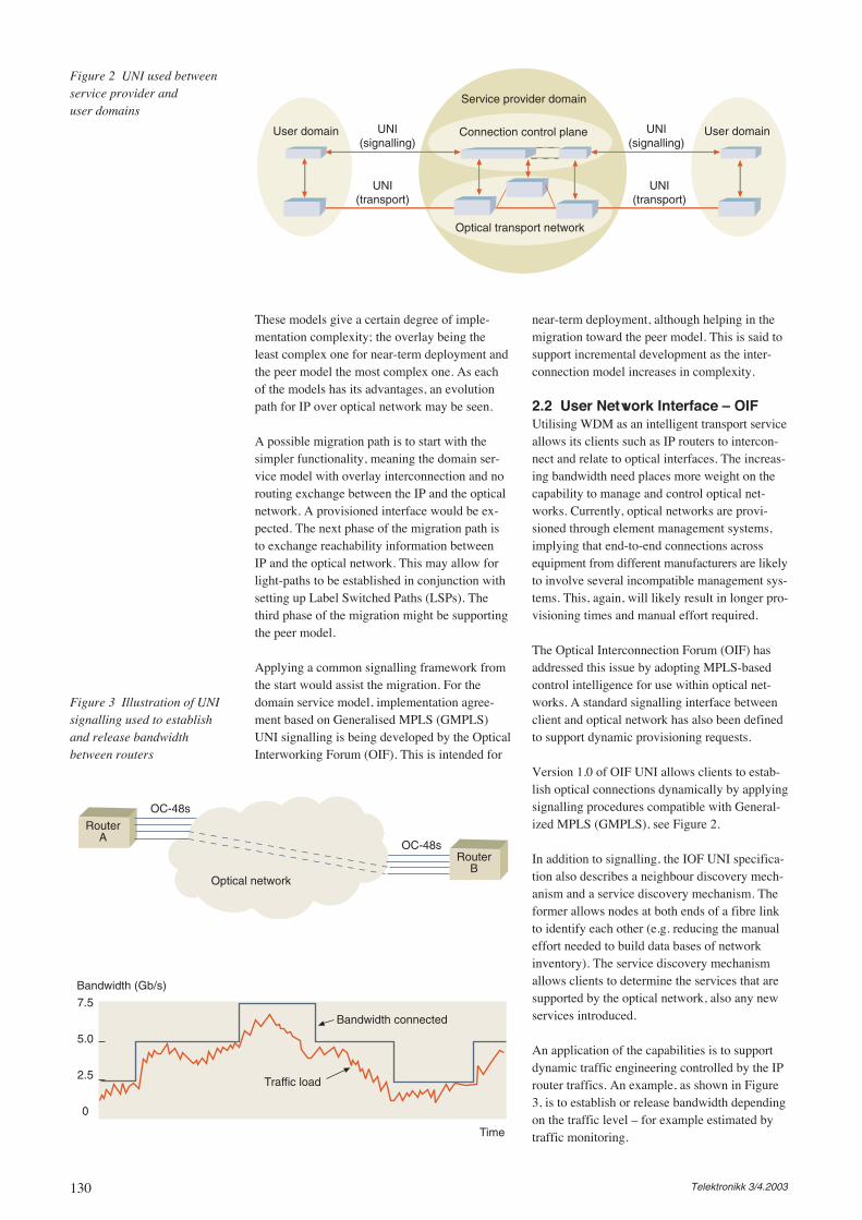
130 Telektronikk 3/4.2003
These models give a certain degree of imple-mentation complexity; the overlay being theleast complex one for near-term deployment andthe peer model the most complex one. As eachof the models has its advantages, an evolutionpath for IP over optical network may be seen.
A possible migration path is to start with thesimpler functionality, meaning the domain ser-vice model with overlay interconnection and norouting exchange between the IP and the opticalnetwork. A provisioned interface would be ex-pected. The next phase of the migration path isto exchange reachability information betweenIP and the optical network. This may allow forlight-paths to be established in conjunction withsetting up Label Switched Paths (LSPs). Thethird phase of the migration might be supportingthe peer model.
Applying a common signalling framework fromthe start would assist the migration. For thedomain service model, implementation agree-ment based on Generalised MPLS (GMPLS)UNI signalling is being developed by the OpticalInterworking Forum (OIF). This is intended for
near-term deployment, although helping in themigration toward the peer model. This is said tosupport incremental development as the inter-connection model increases in complexity.
2.2 User Network Interface – OIFUtilising WDM as an intelligent transport serviceallows its clients such as IP routers to intercon-nect and relate to optical interfaces. The increas-ing bandwidth need places more weight on thecapability to manage and control optical net-works. Currently, optical networks are provi-sioned through element management systems,implying that end-to-end connections acrossequipment from different manufacturers are likelyto involve several incompatible management sys-tems. This, again, will likely result in longer pro-visioning times and manual effort required.
The Optical Interconnection Forum (OIF) hasaddressed this issue by adopting MPLS-basedcontrol intelligence for use within optical net-works. A standard signalling interface betweenclient and optical network has also been definedto support dynamic provisioning requests.
Version 1.0 of OIF UNI allows clients to estab-lish optical connections dynamically by applyingsignalling procedures compatible with General-ized MPLS (GMPLS), see Figure 2.
In addition to signalling, the IOF UNI specifica-tion also describes a neighbour discovery mech-anism and a service discovery mechanism. Theformer allows nodes at both ends of a fibre linkto identify each other (e.g. reducing the manualeffort needed to build data bases of networkinventory). The service discovery mechanismallows clients to determine the services that aresupported by the optical network, also any newservices introduced.
An application of the capabilities is to supportdynamic traffic engineering controlled by the IProuter traffics. An example, as shown in Figure3, is to establish or release bandwidth dependingon the traffic level – for example estimated bytraffic monitoring.
Figure 2 UNI used betweenservice provider anduser domains
Figure 3 Illustration of UNIsignalling used to establishand release bandwidthbetween routers
User domain UNI(signalling)
UNI(transport)
Service provider domain
Connection control plane
Optical transport network
UNI(signalling)
UNI(transport)
User domain
RouterA
RouterB
OC-48s
OC-48s
Optical network
7.5
5.0
2.5
0
Bandwidth (Gb/s)
Traffic load
Bandwidth connected
Time
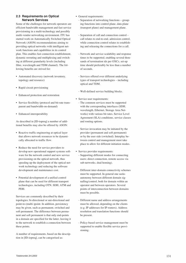
131Telektronikk 3/4.2003
2.3 Requirements on OpticalNetwork Services
Some of the challenges for network operators areefficient bandwidth management and fast serviceprovisioning in a multi-technology and possiblymulti-vendor networking environment. ITU hasstarted work on Automatically Switched OpticalNetwork (ASON) recommendations aiming toproviding optical networks with intelligent net-work functions and capabilities in its controlplan. This enables fast connection establishment,dynamic rerouting and multiplexing and switch-ing at different granularity levels (includingfibre, wavelength and TDM channel). The fol-lowing benefits are strived for:
• Automated discovery (network inventory,topology and resource)
• Rapid circuit provisioning
• Enhanced protection and restoration
• Service flexibility (protocol and bit-rate trans-parent and bandwidth-on-demand)
• Enhanced interoperability
As described in [ID-iopreq] a number of addi-tional benefits may also be offered by ASON:
• Reactive traffic engineering at optical layerthat allows network resources to be dynami-cally allocated to traffic flow.
• Reduce the need for service providers todevelop new operational support systems soft-ware for the network control and new serviceprovisioning on the optical network, thusspeeding up the deployment of the optical net-work technology and reducing the softwaredevelopment and maintenance cost.
• Potential development of a unified controlplane that can be used for different transporttechnologies, including OTN, SDH, ATM andPDH.
Services are commonly described by theirtopologies; bi-directional or uni-directional andpoint-to-(multi-)point. In addition, persistencymay be given, such as permanent, switched andsoft permanent. The difference between perma-nent and soft permanent is that only end-pointsin a domain are specified for the latter, leaving itto the network to establish a connection betweenthese points.
A number of requirements, based on the descrip-tion in [ID-iopreq], can be categorised as:
• General requirements:- Separation of networking functions – group-
ing functions into control plane, data plane(transport plane) and management plane.
- Separation of call and connection control –call relates to end-to-end, admission control,while connection control relates to establish-ing and releasing the connections for a call.
- Network and service scalability and responsetimes to be supported, enabling several thou-sands of termination ids per OXCs, set-uptime should preferably be less than a numberof seconds.
- Services offered over different underlyingtypes of transport technologies – includingoptical and TDM.
- Well-defined service building blocks.
• Service user requirements:- The common services must be supported
with the corresponding interfaces (SDH,wavelength, Ethernet, Storage Area Net-works) with various bit rates, Service LevelAgreement (SLA) conditions, service classesand routing options.
- Service invocation may be initiated by theprovider (permanent and soft permanent)or by the user side (switched). Interplay be-tween control and management must takeplace to allow for different initiation modes.
• Service provider requirements:- Supporting different modes for connecting
users; direct connection, remote access viasub-networks, dual homing).
- Different inter-domain connectivity schemesmust be supported. In general one seeksautonomy between different domain sig-nalling/control, both for domain within anoperator and between operators. Severalpoints of interconnection between domainsmust be possible.
- Different name and address arrangementsmust be allowed, depending on the clients(e.g. IP addresses for IP routers). Addressresolution and translation functions shouldbe present.
- Policy-based service management must besupported to enable flexible service provi-sioning.
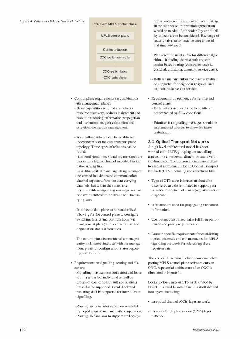
132 Telektronikk 3/4.2003
• Control plane requirements (in combinationwith management plane):- Basic capabilities required are network
resource discovery, address assignment andresolution, routing information propagationand dissemination, path calculation andselection, connection management.
- A signalling network can be establishedindependently of the data transport planetopology. Three types of relations can befound: i) in-band signalling: signalling messages arecarried in a logical channel imbedded in thedata-carrying link; ii) in-fibre, out-of-band: signalling messagesare carried in a dedicated communicationchannel separated from the data-carryingchannels, but within the same fibre; iii) out-of-fibre: signalling messages are car-ried over a different fibre than the data-car-rying links.
- Interface to data plane to be standardisedallowing for the control plane to configureswitching fabrics and port functions (viamanagement plane) and receive failure anddegradation status information.
- The control plane is considered a managedentity and, hence, interacts with the manage-ment plane for configuration, status report-ing and so forth.
• Requirements on signalling, routing and dis-covery:- Signalling must support both strict and loose
routing and allow individual as well asgroups of connections. Fault notificationsmust also be supported. Crank-back andrerouting shall be supported for inter-domainsignalling.
- Routing includes information on reachabil-ity, topology/resource and path computation.Routing mechanisms to support are hop-by-
hop, source-routing and hierarchical routing.In the latter case, information aggregationwould be needed. Both scalability and stabil-ity aspects are to be considered. Exchange ofrouting information may be trigger-basedand timeout-based.
- Path selection must allow for different algo-rithms, including shortest path and con-straint-based routing (constraints such ascost, link utilization, diversity, service class).
- Both manual and automatic discovery shallbe supported for neighbour (physical andlogical), resource and service.
• Requirements on resiliency for service andcontrol plane:- Different service levels are to be offered,
accompanied by SLA conditions.
- Priorities for signalling messages should beimplemented in order to allow for fasterrestoration.
2.4 Optical Transport NetworksA high level architectural model has beenworked on in IETF, grouping the modellingaspects into a horizontal dimension and a verti-cal dimension. The horizontal dimension refersto special requirements for an Optical TransportNetwork (OTN) including considerations like:
• Type of OTN state information should bediscovered and disseminated to support pathselection for optical channels (e.g. attenuation,dispersion).
• Infrastructure used for propagating the controlinformation.
• Computing constrained paths fulfilling perfor-mance and policy requirements.
• Domain specific requirements for establishingoptical channels and enhancements for MPLSsignalling protocols for addressing theserequirements.
The vertical dimension includes concerns whenporting MPLS control plane software onto anOXC. A potential architecture of an OXC isillustrated in Figure 4.
Looking closer into an OTN as described byITU-T, it should be noted that it is itself dividedinto layers, including
• an optical channel (OCh) layer network;
• an optical multiplex section (OMS) layernetwork;
Figure 4 Potential OXC system architectureOXC with MPLS control plane
MPLS control plane
OXC switch fabrc
OXC data plane
Control adaption
OXC switch controller
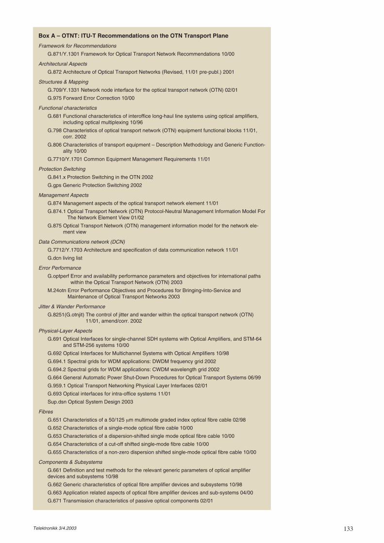
133Telektronikk 3/4.2003
Box A – OTNT: ITU-T Recommendations on the OTN Transport Plane
Framework for Recommendations
G.871/Y.1301 Framework for Optical Transport Network Recommendations 10/00
Architectural Aspects
G.872 Architecture of Optical Transport Networks (Revised, 11/01 pre-publ.) 2001
Structures & Mapping
G.709/Y.1331 Network node interface for the optical transport network (OTN) 02/01
G.975 Forward Error Correction 10/00
Functional characteristics
G.681 Functional characteristics of interoffice long-haul line systems using optical amplifiers,including optical multiplexing 10/96
G.798 Characteristics of optical transport network (OTN) equipment functional blocks 11/01,corr. 2002
G.806 Characteristics of transport equipment – Description Methodology and Generic Function-ality 10/00
G.7710/Y.1701 Common Equipment Management Requirements 11/01
Protection Switching
G.841.x Protection Switching in the OTN 2002
G.gps Generic Protection Switching 2002
Management Aspects
G.874 Management aspects of the optical transport network element 11/01
G.874.1 Optical Transport Network (OTN) Protocol-Neutral Management Information Model ForThe Network Element View 01/02
G.875 Optical Transport Network (OTN) management information model for the network ele-ment view
Data Communications network (DCN)
G.7712/Y.1703 Architecture and specification of data communication network 11/01
G.dcn living list
Error Performance
G.optperf Error and availability performance parameters and objectives for international pathswithin the Optical Transport Network (OTN) 2003
M.24otn Error Performance Objectives and Procedures for Bringing-Into-Service andMaintenance of Optical Transport Networks 2003
Jitter & Wander Performance
G.8251(G.otnjit) The control of jitter and wander within the optical transport network (OTN)11/01, amend/corr. 2002
Physical-Layer Aspects
G.691 Optical Interfaces for single-channel SDH systems with Optical Amplifiers, and STM-64and STM-256 systems 10/00
G.692 Optical Interfaces for Multichannel Systems with Optical Amplifiers 10/98
G.694.1 Spectral grids for WDM applications: DWDM frequency grid 2002
G.694.2 Spectral grids for WDM applications: CWDM wavelength grid 2002
G.664 General Automatic Power Shut-Down Procedures for Optical Transport Systems 06/99
G.959.1 Optical Transport Networking Physical Layer Interfaces 02/01
G.693 Optical interfaces for intra-office systems 11/01
Sup.dsn Optical System Design 2003
Fibres
G.651 Characteristics of a 50/125 µm multimode graded index optical fibre cable 02/98
G.652 Characteristics of a single-mode optical fibre cable 10/00
G.653 Characteristics of a dispersion-shifted single mode optical fibre cable 10/00
G.654 Characteristics of a cut-off shifted single-mode fibre cable 10/00
G.655 Characteristics of a non-zero dispersion shifted single-mode optical fibre cable 10/00
Components & Subsystems
G.661 Definition and test methods for the relevant generic parameters of optical amplifierdevices and subsystems 10/98
G.662 Generic characteristics of optical fibre amplifier devices and subsystems 10/98
G.663 Application related aspects of optical fibre amplifier devices and sub-systems 04/00
G.671 Transmission characteristics of passive optical components 02/01
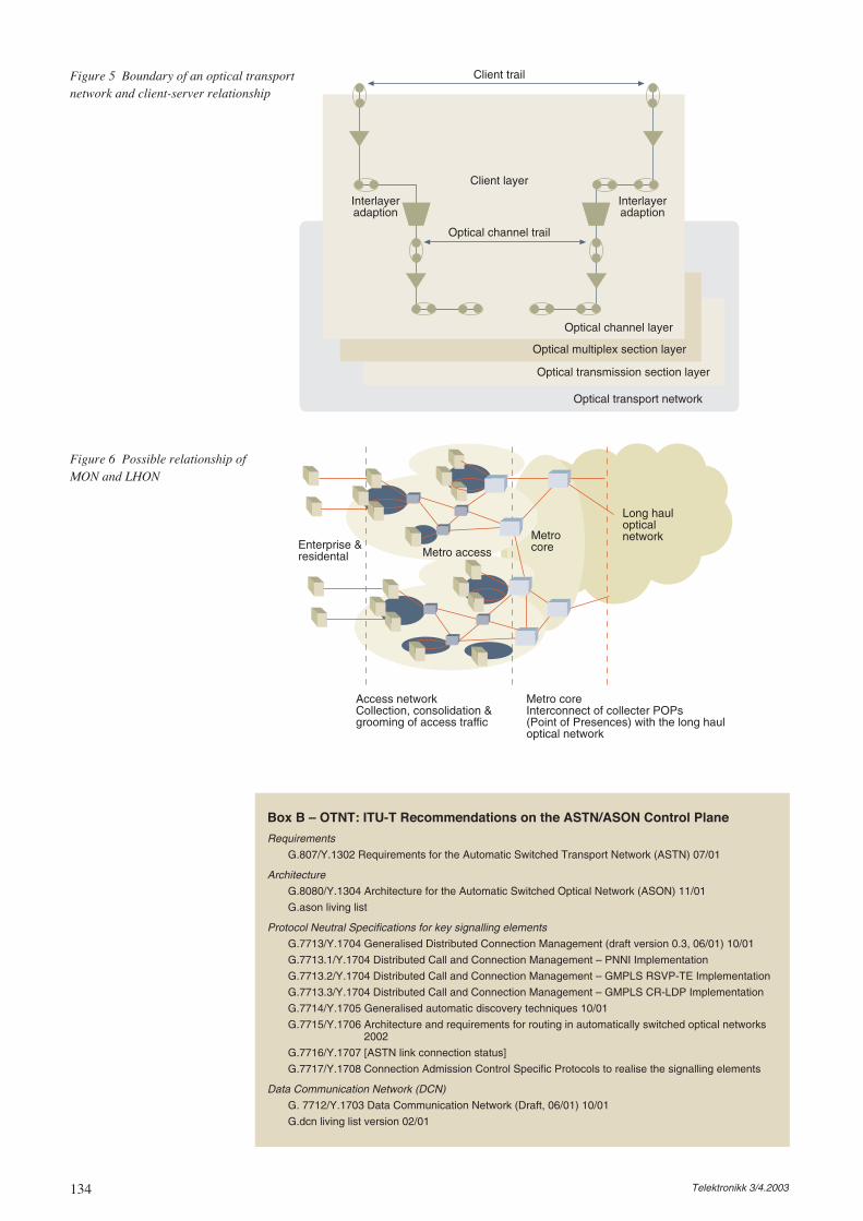
134 Telektronikk 3/4.2003
Box B – OTNT: ITU-T Recommendations on the ASTN/ASON Control Plane
Requirements
G.807/Y.1302 Requirements for the Automatic Switched Transport Network (ASTN) 07/01
Architecture
G.8080/Y.1304 Architecture for the Automatic Switched Optical Network (ASON) 11/01
G.ason living list
Protocol Neutral Specifications for key signalling elements
G.7713/Y.1704 Generalised Distributed Connection Management (draft version 0.3, 06/01) 10/01
G.7713.1/Y.1704 Distributed Call and Connection Management – PNNI Implementation
G.7713.2/Y.1704 Distributed Call and Connection Management – GMPLS RSVP-TE Implementation
G.7713.3/Y.1704 Distributed Call and Connection Management – GMPLS CR-LDP Implementation
G.7714/Y.1705 Generalised automatic discovery techniques 10/01
G.7715/Y.1706 Architecture and requirements for routing in automatically switched optical networks2002
G.7716/Y.1707 [ASTN link connection status]
G.7717/Y.1708 Connection Admission Control Specific Protocols to realise the signalling elements
Data Communication Network (DCN)
G. 7712/Y.1703 Data Communication Network (Draft, 06/01) 10/01
G.dcn living list version 02/01
Figure 6 Possible relationship ofMON and LHON
Interlayeradaption
Interlayeradaption
Client trail
Client layer
Optical channel trail
Optical channel layer
Optical multiplex section layer
Optical transmission section layer
Optical transport network
Figure 5 Boundary of an optical transportnetwork and client-server relationship
Enterprise &residental Metro access
Metrocore
Long haulopticalnetwork
Access networkCollection, consolidation &grooming of access traffic
Metro coreInterconnect of collecter POPs(Point of Presences) with the long hauloptical network
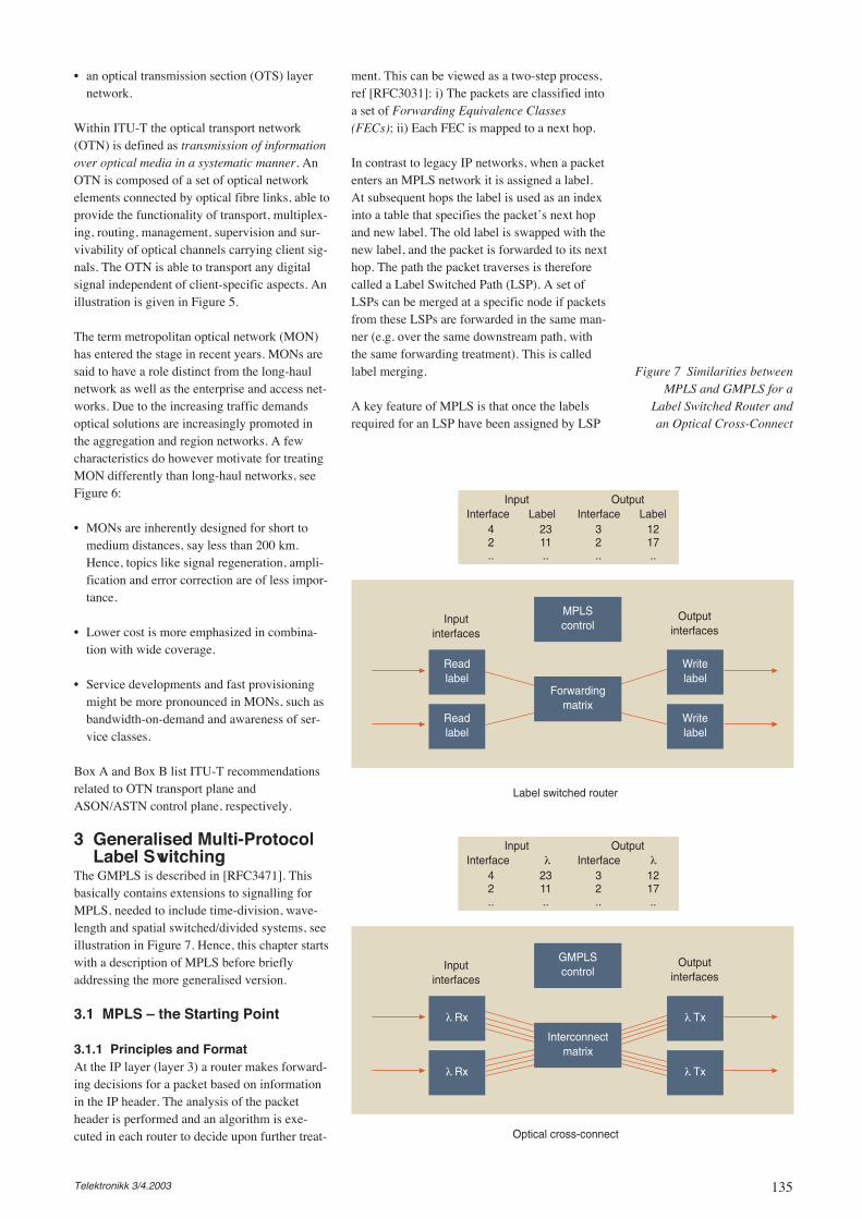
135Telektronikk 3/4.2003
• an optical transmission section (OTS) layernetwork.
Within ITU-T the optical transport network(OTN) is defined as transmission of informationover optical media in a systematic manner. AnOTN is composed of a set of optical networkelements connected by optical fibre links, able toprovide the functionality of transport, multiplex-ing, routing, management, supervision and sur-vivability of optical channels carrying client sig-nals. The OTN is able to transport any digitalsignal independent of client-specific aspects. Anillustration is given in Figure 5.
The term metropolitan optical network (MON)has entered the stage in recent years. MONs aresaid to have a role distinct from the long-haulnetwork as well as the enterprise and access net-works. Due to the increasing traffic demandsoptical solutions are increasingly promoted inthe aggregation and region networks. A fewcharacteristics do however motivate for treatingMON differently than long-haul networks, seeFigure 6:
• MONs are inherently designed for short tomedium distances, say less than 200 km.Hence, topics like signal regeneration, ampli-fication and error correction are of less impor-tance.
• Lower cost is more emphasized in combina-tion with wide coverage.
• Service developments and fast provisioningmight be more pronounced in MONs, such asbandwidth-on-demand and awareness of ser-vice classes.
Box A and Box B list ITU-T recommendationsrelated to OTN transport plane andASON/ASTN control plane, respectively.
3 Generalised Multi-ProtocolLabel Switching
The GMPLS is described in [RFC3471]. Thisbasically contains extensions to signalling forMPLS, needed to include time-division, wave-length and spatial switched/divided systems, seeillustration in Figure 7. Hence, this chapter startswith a description of MPLS before brieflyaddressing the more generalised version.
3.1 MPLS – the Starting Point
3.1.1 Principles and FormatAt the IP layer (layer 3) a router makes forward-ing decisions for a packet based on informationin the IP header. The analysis of the packetheader is performed and an algorithm is exe-cuted in each router to decide upon further treat-
ment. This can be viewed as a two-step process,ref [RFC3031]: i) The packets are classified intoa set of Forwarding Equivalence Classes(FECs); ii) Each FEC is mapped to a next hop.
In contrast to legacy IP networks, when a packetenters an MPLS network it is assigned a label.At subsequent hops the label is used as an indexinto a table that specifies the packet’s next hopand new label. The old label is swapped with thenew label, and the packet is forwarded to its nexthop. The path the packet traverses is thereforecalled a Label Switched Path (LSP). A set ofLSPs can be merged at a specific node if packetsfrom these LSPs are forwarded in the same man-ner (e.g. over the same downstream path, withthe same forwarding treatment). This is calledlabel merging.
A key feature of MPLS is that once the labelsrequired for an LSP have been assigned by LSP
Figure 7 Similarities betweenMPLS and GMPLS for a
Label Switched Router andan Optical Cross-Connect
Input OutputInterface Label Interface Label
42..
2311..
32..
1217..
Inputinterfaces
Outputinterfaces
Readlabel
MPLScontrol
Readlabel
Label switched router
Forwardingmatrix
Writelabel
Writelabel
Input OutputInterface λ Interface
42..
2311..
32..
1217..
Inputinterfaces
Outputinterfaces
λ Rx
GMPLScontrol
Interconnectmatrix
λ
λ Rx
λ Tx
λ Tx
Optical cross-connect
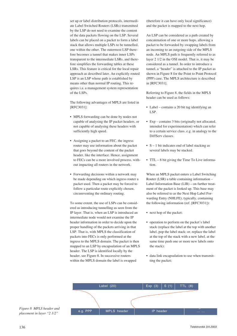
136 Telektronikk 3/4.2003
set up or label distribution protocols, intermedi-ate Label Switched Routers (LSRs) transmittedby the LSP do not need to examine the contentof the data packets flowing on the LSP. Severallabels can be placed on a packet to form a labelstack that allows multiple LSPs to be tunnelled,one within the other. The outermost LSP there-fore becomes a tunnel that makes inner LSPstransparent to the intermediate LSRs, and there-fore simplifies the forwarding tables at theseLSRs. This feature is critical for the local repairapproach as described later. An explicitly routedLSP is an LSP whose path is established bymeans other than normal IP routing. This re-quires i.a. a management system representationof the LSPs.
The following advantages of MPLS are listed in[RFC3031]:
• MPLS forwarding can be done by nodes notcapable of analysing the IP packet headers, ornot capable of analysing these headers withsufficiently high speed.
• Assigning a packet to an FEC, the ingressrouter may use information about the packetthat goes beyond the content of the packetheader, like the interface. Hence, assignmentto FECs can be a more involved process, with-out impacting all routers in the network.
• Forwarding decisions within a network maybe made depending on which ingress router apacket used. Then a packet may be forced tofollow a particular route explicitly chosen,circumventing the ordinary routing.
To some extent, the use of LSPs can be consid-ered as introducing tunnelling as seen from theIP layer. That is, when an LSP is introduced anintermediate node would not examine the IPheader information in order to decide upon theproper handling of the packets arriving in thatLSP. That is, with MPLS the classification ofpackets into FECs is only performed at theingress to the MPLS domain. The packet is thenmapped to an LSP by encapsulation of an MPLSheader. The LSP is identified locally by theheader, see Figure 8. In successive routerswithin the MPLS domain the label is swapped
Figure 8 MPLS header andplacement in layer “2 1/2”
(therefore it can have only local significance)and the packet is mapped to the next hop.
An LSP can be considered as a path created byconcatenation of one or more hops, allowing apacket to be forwarded by swapping labels froman incoming to an outgoing side of the MPLSnode. An MPLS path is frequently referred to aslayer 2 1/2 in the OSI model. That is, it may beconsidered as a tunnel. In order to introduce atunnel, a “header” is attached to the IP packet asshown in Figure 8 for the Point to Point Protocol(PPP) case. The MPLS architecture is describedin [RFC3031].
Referring to Figure 8, the fields in the MPLSheader can be used as follows:
• Label – contains a 20 bit tag identifying anLSP.
• Exp – contains 3 bits (originally not allocated,intended for experimentation) which can referto a certain service class, e.g. in analogy to theDiffServ classes.
• S – 1 bit indicates end of label stacking asseveral labels may be stacked.
• TTL – 8 bit giving the Time To Live informa-tion.
When an MPLS packet enters a Label SwitchingRouter (LSR) a table containing information –Label Information Base (LIB) – on further treat-ment of the packet is looked up. This base mayalso be referred to as the Next Hop Label For-warding Entry (NHLFE), typically, containingthe following information (ref. [RFC3031]):
• next hop of the packet;
• operation to perform on the packet’s labelstack (replace the label at the top with anotherlabel, pop the label stack; or, replace the labelat the top of the stack with a new label, at thesame time push one or more new labels ontothe stack);
• data link encapsulation to use when transmit-ting the packet;
Label (20) Exp (3) S (1) TTL (8)
e.g. PPP MPLS header IP header … …
137Telektronikk 3/4.2003
• way of encoding the label stack when trans-mitting the packet;
• other information relevant for forwardingtreatment.
In a given LSR, the “next hop LSR” may be thesame LSR, implying that the top level labelshould be popped and the packet “forwarded” toitself, allowing for more forwarding decisions.
At the ingress of an MPLS domain an FEC-to-NHLFE mapping is needed; that is when packetsarrive without an MPLS label.
Within an MPLS domain an incoming labelmapping is executed, mapping the packet ontoa set of NHLFEs.
MPLS can operate on a label stack. Operationson this stack are push, pop and swap. This canbe used to merge and split traffic streams. Thepush operation adds a new label at the top of thestack and the pop operation removes one labelfrom the stack. The MPLS stack functionalitycan be used to aggregate traffic trunks. A com-mon label is added to the stack of labels. Theresult is an aggregated trunk. When this MPLSpath is terminated the result will be a splitting(de-aggregation) of the aggregated trunk intoits individual components. Two trunks can beaggregated in this way if they share a portion oftheir path. Hence, MPLS can provide hierarchi-cal forwarding, potentially becoming an impor-tant feature. A consequence may be that the tran-sit provider need not carry global routing infor-mation, thus making the MPLS network morestable and scalable than a full-blown routed net-work.
3.1.2 Traffic Engineering and MPLSWhen utilising MPLS with Traffic Engineering,a number of mapping relations is asked for:
• Mapping packets onto FECs. An FEC com-poses a group of packets to be forwarded overthe same path with the same forwarding treat-ment. In order to carry out this mapping fieldsin the IP packet are examined.
• Mapping FECs onto traffic trunks. A traffictrunk is an aggregation of traffic flows of thesame class. A traffic trunk can again be routed(placed inside an LSP; i.e. a traffic trunk isonly given for one LSP and not a sequence ofLSPs).
• Mapping traffic trunks onto LSPs.
• Mapping LSPs onto links in the physical net-work.
In several sources, the terms traffic trunk andLSP are used synonymously. A fundamentaldifference between traffic trunk and LSP can beobserved, though. That is, a traffic trunk is anabstract representation of traffic to which spe-cific characteristics can be associated. An LSPis a description of a path in the network throughwhich the traffic traverses.
Trunks having the same egress point may bemerged into a common tree towards the egress.This may reduce the number of trees signifi-cantly. Trunks can also be aggregated by addinga new label to the stack for each trunk (that is,bundling the trunks into a single path/tunnel).
Designing an MPLS network “on top of” a phys-ical network could be looked upon as relatingtwo graphs to each other:
• Physical graph, G = (V, E, c) is a capacitatedgraph depicting the physical topology of thenetwork. V is the set of nodes in the networkand E is the set of links. For v to w in V, (v, w)represents the link in E when v and w aredirectly connected under G. c indicates the setof capacity and other constraints associatedwith E and V.
• MPLS graph, H = (U, F, d), where U is a sub-set of V representing the LSRs; that is the setof LSRs that are endpoint of at least one LSP.F is the set of LSPs. For x and y in U, (x, y) isin F if there is an LSP going from x to y. drepresents the set of demands and restrictionsassociated with F.
The fundamental problem of designing an MPLSnetwork is to relate the two graphs such that anobjective function is optimised.
One of the requirements from Traffic Engineer-ing is to be able to reroute an LSP under a num-ber of conditions (failure, better route available,etc.). It is desirable that this is done without dis-turbing the traffic flows. This could be done byestablishing the new LSP before the old/existingLSP is released, which is called make-before-break. In case the existing and new LSP competefor the same resources, particular concerns haveto be made, also considered by the admissioncontrol.
In addition to attributes related to traffic trunks,see Box C, some attributes are also related toresources (frequently thought of as the links).These attributes are ([RFC2702]):
• Maximum allocation multiplier attribute. Thevalue of this attribute tells what proportion ofthe link and buffer capacity is available. Then,

138 Telektronikk 3/4.2003
“over-allocation” could be achieved (as wellas “under-allocation”).
• Resource class attributes. The attributesexpress the resource type (e.g. thought of ascolours). These are matched with the traffictrunk affinity attribute when finding pathsonto which the traffic trunks are routed.
Basic operations on traffic trunks are([RFC2702]):
• Establish a traffic trunk• Activate a traffic trunk, to start passing packets• Deactivate a traffic trunk• Modify attributes for a traffic trunk• Reroute a traffic trunk• Remove a traffic trunk.
In addition to these basic operations, a few more,like policing and shaping could also be defined.
A traffic trunk is defined as unidirectional. Asa bidirectional transfer capability is commonlyasked for, two traffic trunks having the sameend-points but passing packets in opposite direc-tions can be defined. In case these are alwayshandled as a unit, it is called a bidirectional traf-fic trunk (they are established as an atomic oper-ation and one may not exist without the other).If a trunk is routed through a different physicalpath from the corresponding trunk in the oppo-site direction, the bidirectional traffic trunk iscalled topological asymmetric. Otherwise, it iscalled topological symmetric.
3.2 GMPLS Multiplexing HierarchyMPLS uses labels to support forwarding ofpackets. Label Switching Routers (LSRs) havea forwarding table recognising the cells/frameswith the labels, or the IP packet headers (at theborder of the MPLS domain). This is extendedin GMPLS where the following interfaces aregiven for an LSR:
• Interfaces that recognise packet/cell/frameboundaries and forward the data based on thecontent in the packet or label/cell header. Thisis referred to as Packet-Switch Capable. Ex-amples are MPLS-capable routers and ATMswitches.
• Interfaces that forward data based on time slotin a periodic cycle. This is referred to as Time-Division Multiplex Capable. SDH cross-con-nect is one example.
• Interfaces that forward data based on thewavelength. Such interfaces are referred toas Lambda Switch Capable. An optical cross-connect is an example.
• Interfaces that forward data based on physicalspace position of data. This is referred to asFibre-Switch Capable. An optical cross-con-nect operating on a level of single or multiplefibres is an example.
These can be organised in a hierarchical manneras shown in Figure 9 and corresponding labelsand Label Switched Paths (LSPs) defined. Then,
Figure 9 Organising “labels”hierarchically
Box C – Attributes characterising traffic trunks are ([RFC2702]):
• Traffic parameter attributes. These are used to describe the traffic flows (theFECs) transported in the traffic trunk. Relevant parameters include peak rates,average rates, maximal burst size, etc. Possibly, equivalent measures could beapplied, like the effective bandwidth.
• Explicit path specification attribute. An explicit path assignment for a traffictrunk is a path that is specified through “operator” action (e.g. managementprocedures). Such a path can be completely or partially specified. Path prefer-ence rules may be associated with explicit paths, telling whether the explicitpath is “mandatory” (has to be followed) or “optional” (other paths could beselected in case sufficient resources are not available on the preferred path).
• Resource class affinity attribute. This attribute can be used to specify whichresource types can be explicitly included or excluded from the path throughwhich the traffic trunk is routed. If no affinity attribute is given a “don’t care”condition is assumed. Routing traffic trunks onto resources has to take theseattributes into account, matching the requirements.
• Adaptivity attribute. As network state and traffic state change over time, moreoptimal routes of traffic trunks could appear. Setting this attribute tells whetheror not the route can be re-optimised for the traffic trunk. However, appropriatethresholds should be given avoiding too frequent changes of routing.
• Load distribution attribute. In case several traffic trunks are used between thepair of nodes, the load distribution attribute can tell whether or not the load(traffic trunk) can be distributed on these trunks. In general the packet ordershould be maintained, implying that packets belonging to the same traffic floware transferred on the same traffic trunk.
• Priority attribute. This attribute gives the relative importance of the traffic trunk.The value can be used to determine the order in which trunks are assigned topaths under establishment and failure situations. Priorities will also be usedtogether with preemption.
• Preemption attribute. The value of this attribute tells whether or not a traffictrunk can preempt another traffic trunk, and whether or not another traffic trunkcan preempt a specific traffic trunk. This will assist to ensure that high prioritytraffic trunks are routed through even though the capacity is not sufficient tohandle all traffic trunks.
• Resilience attribute. The resilience attribute gives the behaviour of a traffictrunk when faults occur along the path followed by a traffic trunk. In case offault the traffic trunk could be rerouted or not depending on the value of thisattribute. For rerouting, the constraints given (e.g. by affinity) could be observedor not.
• Policing attribute. The value of this attribute tells which actions to take when thetraffic on the trunk is not complying (traffic is exceeding). Examples of actionsare packet dropping (rate limiting), packet tagging and packet shaping.
IP packet packet-switchtime-division
multiplexlambdaswitch
fibreswitch
139Telektronikk 3/4.2003
an LSP that starts and ends on a packet-switchcapable interface can be grouped together withother similar LSPs into a common LSP thatstarts and ends on a time-division multiplexinterface. This LSP can be grouped together withother similar LSPs into an LSP that starts andends on a lambda switch capable interface, andso forth. This is similar to a multiplexing hierar-chy. Note that all these levels may not be presentin all cases.
Compared with MPLS, the GMPLS introducesadditional interface types. The formats of thelabels on the interfaces are given in [RFC3471].
Motivations for combining solutions for MPLS,in particular related to Traffic Engineering, andmechanisms for control plane in OXCs are:
• to provide a framework for real-time provi-sioning of optical channels in automaticallyswitched optical networks;
• to foster the expedited development anddeployment of a new class of versatile OXCs;
• to allow the use of uniform semantics for net-work management and operation control andhybrid networks consisting of OXCs and labelswitching routers (LSRs).
A particular emphasis may be placed on supportof various protection and restoration schemes.
3.3 GMPLS Signalling FunctionalDescription
Extensions to MPLS signalling to supportGMPLS are described in [RFC3471]. A general-ized label contains sufficient information for areceiving node to program its cross connectfabric. Between nodes generalized labels areexchanged in order to allow these nodes to knowhow to handle the information attached withthese labels in the next phase. Generalized labelrequests are used consisting of
• 8 bit LSP encoding type: gives the LSP types,such as 1 = packet, 2 = Ethernet, 5 = SDH,8 = lambda, 9 = fibre
• 8 bit switching type: gives the type of switch-ing (packet switch, layer 2 switch, TDMswitch, lambda switch, fibre switch)
• 16 bit Generalized payload identifier: givesthe type of client layer to the LSP (IP, MPLS,Ethernet, SDH, lambda, fibre)
The label itself depends on the link type it isreferring to. For fibre and lambda a 32 bit labelhas been described being significant betweentwo neighbour nodes. Allowing for a range of
(close-by) lambdas to be switched along thesame route a waveband label has been devised,giving the start and end label (and thereby therange of wavelengths to be routed together).
GMPLS allows for bi-directional LSPs to beestablished as an atomic activity (compared withhaving to set up two uni-directional LSPs forMPLS). This allows for reduced set-up times,although one label each has to be assigned in thedifferent directions.
Link-related protection can also be carried by thesignalling field called Protection Information.The use of this field is optional. The protectioncapabilities of a link may be advertised by therouting scheme. The Protection Information fieldalso indicates whether the LSP is primary or sec-ondary (backup). The resources of the secondaryLSP may be used by other LSPs until the pri-mary LSP fails over to the secondary LSP.
The Protection Information field consists ofthree units:
• 1 bit secondary flag – set to 1 for a secondaryLSP
• 25 bit reserved (set to zero)
• 6 bit link flags – indicates protection type (e.g.1 + 1, 1 : 1, shared, unprotected)
4 Single-Layer SurvivabilityFour options exist for a two-layer structure ifeach of the layers is considered in isolation:i) no survivability mechanism; ii) survivabilitymechanisms in the lower layer; iii) survivabilitymechanisms in the upper layer; and iv) surviv-ability mechanisms both in the lower and upperlayer, but without any coordination. The firstoption is of little relevance for this discussion.Factors to be considered for the others are(adapted from [Coll02]):
• Lower layer survivability only: A basic advan-tage for having recovery mechanisms in thelower layer is that simple root failure has tobe treated and recovery actions are performedon the coarsest granularity. This results in thelowest number of required recovery actions.Moreover, failures do not need to propagatethrough other layers before triggering anyrecovery actions. A drawback, however, isthat failure in upper layers may not be re-solved. In addition, when a failure occurs in alower layer node, this layer recovers affectedtraffic where this node is involved, possiblyleaving upper layer nodes in isolation (seeFigure 10).
140 Telektronikk 3/4.2003
• Upper layer survivability only: An advantageof upper layer survivability is that it can han-dle node or higher layer failures more easily.A disadvantage is that several recovery ac-tions may be needed because of finer granular-ity of the traffic flows in the upper layer, seeFigure 11. On the other hand, this finer granu-larity allows for a differentiation of trafficflows, both in speed of recovery and decisionon whether or not recovery actions should beactivated. In some cases finer granularitymight also lead to more efficient capacityusage. One cause of this is that aggregatedflows (at lower layer), poorly filled withworking traffic flows, may have quite a lot ofspare resources. A second cause is that finergranularity allows distributing flows on morealternative paths.
• Single layer survivability combinations:A number of variants considering recoverymechanisms in different layers can also beincluded under the single layer survivability.The argument is that for each failure scenario,the responsibility to recover traffic is the situ-ation on only one layer. A variant to the aboveis survivability at the lowest detecting layer.That is in a multi-layer configuration, the(single) layer detecting the (root) failure is the
only layer taking any recovery actions. Hence,a failure in a higher layer node will then bedetected and dealt with in that layer. A situa-tion depicted in Figure 10 may still not behandled. Another variant is survivability at thehighest possible layer. This addresses the situ-ations where traffic flows are injected at dif-ferent layers (e.g. combination of opticalchannels, SDH-based leased lines and IP traf-fic flows). A recovery strategy could be todeal with failures at the layers where the dif-ferent traffic flows are injected.
5 Multi-Layer SurvivabilityA common design goal for a network with multi-ple technological layers is to provide the desiredlevel of service in the most cost-effective man-ner. Multi-layer survivability may allow theoptimisation of spare resources through theimprovement of resource utilization by sharingspare capacity across different layers. Coordina-tion during recovery among different networklayers might necessitate the development of avertical hierarchy. The benefits of proving sur-vivability mechanisms at multiple layers and theoptimisation to the overall approach must beweighed with the associated cost and serviceimpacts.
Figure 10 Only recoverymechanisms in the lower layermay result in isolated upperlayer nodes
Figure 11 Single failure atlower layer may result inseveral failure indications atupper layer
a c
d
e
f
A
B
C
D
E
F
b
a c
d
e
f
A
B
C
D
E
F
b
141Telektronikk 3/4.2003
A default coordination mechanism for inter-layerinteraction could be the use of nested timers andcurrent SDH fault monitoring, as has been donetraditionally for backward compatibility. Thus,when lower-layer recovery happens in a longertime period than higher-layer recovery, a hold-off timer is utilized to avoid contention betweenthe different single-layer survivability schemes.In other words, multiplayer interaction isaddressed by having successively higher multi-plexing levels operate at a protection/restorationtime scale greater than the net lowest layer. Thiscan impact the overall time to restore service.For example, if SDH protection switching isused, MPLS recovery timers must wait untilSDH has had time to switch. Setting such timersinvolves a trade-off between rapid recovery andcreation of a race condition where multiple lay-ers are responding to the same fault, potentiallyallocating resources in an inefficient manner.
In other configurations where the lower layerdoes not have a restoration capability or is notexpected to protect, say an unprotected SDH lin-ear circuit, then there must be a mechanism forthe lower layer to trigger the higher layer to takerecovery action immediately. This differencein network configuration means that implemen-tations must allow for adjustment of hold-offtimer values and/or a means for the lower layerto immediately indicate to a higher layer that thefault has occurred so that the higher layer cantake restoration or protection actions.
Moreover, faults at higher layers should nottrigger restoration or protection actions at lowerlayers.
The fact that there are a number of layers presentraises the question of whether these could beutilised in a coordinated manner to improvethe recovery schemes. Three main classes ofschemes are:
• Uncoordinated approach: This may be con-sidered as the simplest approach, that is to
install recovery mechanisms in several layers,but without any coordination between them.An advantage is that it is simple to install andoperate. A main disadvantage is that eachrecovery mechanism requires spare resources.This implies that spare resources are seen foreach layer (and the overall situation could befairly low resource utilisation). Moreover,more extra traffic (that is pre-emptable andunprotected) could be disrupted during a fail-ure. An example (Figure 12) is where thelower layer switches traffic from a workinglink to a recovery path and hence pre-emptsextra traffic on that link. However, the upperlayer may gradually route the traffic onanother path (possibly also pre-empting addi-tional traffic along that path). For the examplein Figure 12 link A – D fails and the lowerlayer moves traffic to links A – B – D. How-ever, the upper layer may find that anotherpath is better so the traffic is effectivelymoved onto links A – C – E (potentially re-sulting in poor utilisation of links A – B – D).
• Sequential approach: Realising that somecoordination would likely result in improvedutilisation, different options are investigated.The next level of complexity is seen where theresponsibility for recovery is handed over tothe next layer when it is clear that the currentlayer is not able to fulfil the recovery task. Inprinciple any sequence of layers can bethought of, however, two obvious ones arebottom-up and top-down. For the former thelowest detecting layer starts the recovery andtraffic that cannot be resolved by this layer(e.g. due to capacity shortage) will be restoredby a higher layer. This has the advantage thatrecovery actions are taken at the appropriategranularity and more complex secondary fail-ures are only treated when needed. For thetop-down approach the upper layer starts therecovery action and only if that layer is unableto restore all traffic are actions at lower layersinitiated. An advantage of this is that higherlayers may differentiate traffic due to require-
Figure 12 Illustration ofuncoordinated recovery; lowerlayer routes on neighbour link,while upper layer may find thatanother path is better
a c
de
A
B
C
DE
b
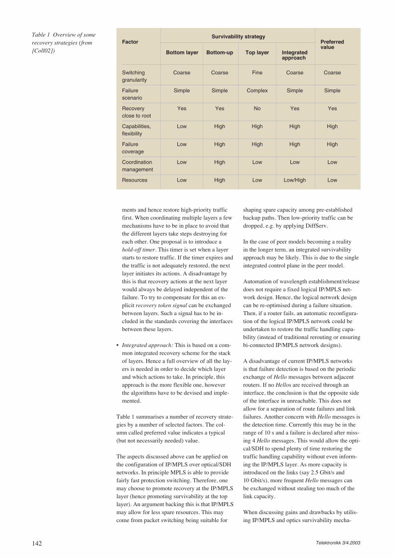
142 Telektronikk 3/4.2003
ments and hence restore high-priority trafficfirst. When coordinating multiple layers a fewmechanisms have to be in place to avoid thatthe different layers take steps destroying foreach other. One proposal is to introduce ahold-off timer. This timer is set when a layerstarts to restore traffic. If the timer expires andthe traffic is not adequately restored, the nextlayer initiates its actions. A disadvantage bythis is that recovery actions at the next layerwould always be delayed independent of thefailure. To try to compensate for this an ex-plicit recovery token signal can be exchangedbetween layers. Such a signal has to be in-cluded in the standards covering the interfacesbetween these layers.
• Integrated approach: This is based on a com-mon integrated recovery scheme for the stackof layers. Hence a full overview of all the lay-ers is needed in order to decide which layerand which actions to take. In principle, thisapproach is the more flexible one, howeverthe algorithms have to be devised and imple-mented.
Table 1 summarises a number of recovery strate-gies by a number of selected factors. The col-umn called preferred value indicates a typical(but not necessarily needed) value.
The aspects discussed above can be applied onthe configuration of IP/MPLS over optical/SDHnetworks. In principle MPLS is able to providefairly fast protection switching. Therefore, onemay choose to promote recovery at the IP/MPLSlayer (hence promoting survivability at the toplayer). An argument backing this is that IP/MPLSmay allow for less spare resources. This maycome from packet switching being suitable for
shaping spare capacity among pre-establishedbackup paths. Then low-priority traffic can bedropped, e.g. by applying DiffServ.
In the case of peer models becoming a realityin the longer term, an integrated survivabilityapproach may be likely. This is due to the singleintegrated control plane in the peer model.
Automation of wavelength establishment/releasedoes not require a fixed logical IP/MPLS net-work design. Hence, the logical network designcan be re-optimised during a failure situation.Then, if a router fails, an automatic reconfigura-tion of the logical IP/MPLS network could beundertaken to restore the traffic handling capa-bility (instead of traditional rerouting or ensuringbi-connected IP/MPLS network designs).
A disadvantage of current IP/MPLS networksis that failure detection is based on the periodicexchange of Hello messages between adjacentrouters. If no Hellos are received through aninterface, the conclusion is that the opposite sideof the interface in unreachable. This does notallow for a separation of route failures and linkfailures. Another concern with Hello messages isthe detection time. Currently this may be in therange of 10 s and a failure is declared after miss-ing 4 Hello messages. This would allow the opti-cal/SDH to spend plenty of time restoring thetraffic handling capability without even inform-ing the IP/MPLS layer. As more capacity isintroduced on the links (say 2.5 Gbit/s and10 Gbit/s), more frequent Hello messages canbe exchanged without stealing too much of thelink capacity.
When discussing gains and drawbacks by utilis-ing IP/MPLS and optics survivability mecha-
Survivability strategyFactor Preferred
valueBottom layer Bottom-up Top layer Integrated
approach
Switching Coarse Coarse Fine Coarse Coarsegranularity
Failure Simple Simple Complex Simple Simplescenario
Recovery Yes Yes No Yes Yesclose to root
Capabilities, Low High High High Highflexibility
Failure Low High High High Highcoverage
Coordination Low High Low Low Lowmanagement
Resources Low High Low Low/High Low
Table 1 Overview of somerecovery strategies (from[Coll02])
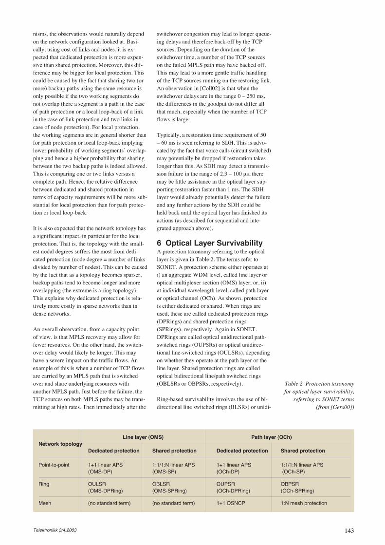
143Telektronikk 3/4.2003
nisms, the observations would naturally dependon the network configuration looked at. Basi-cally, using cost of links and nodes, it is ex-pected that dedicated protection is more expen-sive than shared protection. Moreover, this dif-ference may be bigger for local protection. Thiscould be caused by the fact that sharing two (ormore) backup paths using the same resource isonly possible if the two working segments donot overlap (here a segment is a path in the caseof path protection or a local loop-back of a linkin the case of link protection and two links incase of node protection). For local protection,the working segments are in general shorter thanfor path protection or local loop-back implyinglower probability of working segments’ overlap-ping and hence a higher probability that sharingbetween the two backup paths is indeed allowed.This is comparing one or two links versus acomplete path. Hence, the relative differencebetween dedicated and shared protection interms of capacity requirements will be more sub-stantial for local protection than for path protec-tion or local loop-back.
It is also expected that the network topology hasa significant impact, in particular for the localprotection. That is, the topology with the small-est nodal degrees suffers the most from dedi-cated protection (node degree = number of linksdivided by number of nodes). This can be causedby the fact that as a topology becomes sparser,backup paths tend to become longer and moreoverlapping (the extreme is a ring topology).This explains why dedicated protection is rela-tively more costly in sparse networks than indense networks.
An overall observation, from a capacity pointof view, is that MPLS recovery may allow forfewer resources. On the other hand, the switch-over delay would likely be longer. This mayhave a severe impact on the traffic flows. Anexample of this is when a number of TCP flowsare carried by an MPLS path that is switchedover and share underlying resources withanother MPLS path. Just before the failure, theTCP sources on both MPLS paths may be trans-mitting at high rates. Then immediately after the
switchover congestion may lead to longer queue-ing delays and therefore back-off by the TCPsources. Depending on the duration of theswitchover time, a number of the TCP sourceson the failed MPLS path may have backed off.This may lead to a more gentle traffic handlingof the TCP sources running on the restoring link.An observation in [Coll02] is that when theswitchover delays are in the range 0 – 250 ms,the differences in the goodput do not differ allthat much, especially when the number of TCPflows is large.
Typically, a restoration time requirement of 50– 60 ms is seen referring to SDH. This is advo-cated by the fact that voice calls (circuit switched)may potentially be dropped if restoration takeslonger than this. As SDH may detect a transmis-sion failure in the range of 2.3 – 100 µs, theremay be little assistance in the optical layer sup-porting restoration faster than 1 ms. The SDHlayer would already potentially detect the failureand any further actions by the SDH could beheld back until the optical layer has finished itsactions (as described for sequential and inte-grated approach above).
6 Optical Layer SurvivabilityA protection taxonomy referring to the opticallayer is given in Table 2. The terms refer toSONET. A protection scheme either operates ati) an aggregate WDM level, called line layer oroptical multiplexer section (OMS) layer; or, ii)at individual wavelength level, called path layeror optical channel (OCh). As shown, protectionis either dedicated or shared. When rings areused, these are called dedicated protection rings(DPRings) and shared protection rings(SPRings), respectively. Again in SONET,DPRings are called optical unidirectional path-switched rings (OUPSRs) or optical unidirec-tional line-switched rings (OULSRs), dependingon whether they operate at the path layer or theline layer. Shared protection rings are calledoptical bidirectional line/path switched rings(OBLSRs or OBPSRs, respectively).
Ring-based survivability involves the use of bi-directional line switched rings (BLSRs) or unidi-
Line layer (OMS) Path layer (OCh)Network topology
Dedicated protection Shared protection Dedicated protection Shared protection
Point-to-point 1+1 linear APS 1:1/1:N linear APS 1+1 linear APS 1:1/1:N linear APS(OMS-DP) (OMS-SP) (OCh-DP) (OCh-SP)
Ring OULSR OBLSR OUPSR OBPSR(OMS-DPRing) (OMS-SPRing) (OCh-DPRing) (OCh-SPRing)
Mesh (no standard term) (no standard term) 1+1 OSNCP 1:N mesh protection
Table 2 Protection taxonomyfor optical layer survivability,
referring to SONET terms(from [Gers00])
144 Telektronikk 3/4.2003
rectional path-switched rings (UPSRs) as self-protecting transmission system overlaid on thenetwork topology. More recent variants ofUPSR- and BLSR-based transport networks areoptical path protection ring (OPPR) and opticalshared protection ring (OSPR) variants in aWDM context. An important factor is that ringsmay use simple switching mechanisms, whichpermits restoration in about 50 – 60 ms, althoughby nature they require 100 % redundancy. Inparticular, the BLSR uses a working-to-protec-tion loop-back switching mechanisms at the twonodes adjacent to a failure. In essence, this isidentical to the switching mechanism employedfor p-cycles (in WDM or SDH). According to[Stam00], in conventional multi-ring networkdesigns, where the working fibres of channelgroups are not fully utilizable, effective protec-tion-to-working capacity ratios (capacity redun-dancy) can be 200 – 300 %. This may show thatrings allow fast restoration but may not becapacity-efficient.
Mesh-based survivability is more capacity-effi-cient due to the fact that each unit of sparecapacity can be used in several manners, i.e. forseveral failures. Hence, overall performanceclose to the ideal maximum-flow routing-effi-ciency can be realised. Mesh restoration has tra-ditionally been based on cross-connect systemsembedded in a mesh-like set of point-to-pointtransmission systems. This is one factor forslower restoration compared with ring systems.In addition comes the more general nature ofsolving a capacitated multiple-path reroutingproblem for mesh networks compared withrings.
Hence, mesh and ring both have their strengthsand weaknesses. Mesh networks tend to be app-lied in the long-haul networks where capacity ontransmission links is expensive. Rings tend to bemore cost-efficient in the metro areas where costis dominated by terminal equipment and not somuch with the link and through-connect (due toshort links). A method named p-cycle has beenpromoted trying to merge the advantages of ringand mesh. p-cycles are based on the formation ofclosed paths (elementary cycles in graph theo-retic terms), called p-cycles, in the protectioncapacity of a mesh-restorable network. They areformed in advance of any failure, out of the pre-viously unconnected protection capacity units ofa restorable network. A p-cycle protects both on-cycle and straddling failures (the latter refers topaths not following the cycle during normalworking situation, but may follow the cycle dur-ing failure of any link not being part of thecycle). This implies that protection capacity on ap-cycle is more widely accessible, i.e. morehighly shared for restoration compared with tra-ditional rings. Still, the cycle formation allows
for fast restoration. Moreover, a few cases (e.g.ref. [Stam00]) show that p-cycles can be aboutas capacity-efficient as mesh networks. Com-pared to rings, p-cycles also de-couple the rout-ing of working and protecting paths by the factthat the working paths may be routed along theshortest paths, while protecting paths follow thecycle.
The reason for p-cycles being as fast as rings isthat only two traffic-substituting connections aremade for any working path failure to be restored.The two end nodes perform the switching onlyby transmitting a control signal as they know inadvance which working-to-protection functionsare needed for any given failure. p-cycles can beintroduced, in principle, on optical, SDH, andMPLS layers.
It is quite common to find mesh physical topolo-gies in the backbone networks. The SDH layerplaced on that, however, is in most cases pro-tected in the form of rings. These rings are inter-connected to provide an overall network connec-tivity and protection. It is a question whetherthese schemes are less bandwidth efficient toprotect a physical meshed network. Efficiencyimprovements in the area 20 – 60 % have beendemonstrated by introducing mesh protectionschemes, although these observations naturallydepend on the topology, traffic patterns and pro-tection scheme. Taxonomy of mesh protectionvariations including trade-offs between them asdepicted in Figure 13.
Deploying a robust mesh protection scheme, anumber of challenges have to be met (adaptedfrom [Gers00]):
• A fast signalling mechanism is needed topropagate information about failure events torelevant nodes so they can reconfigure theswitches to accommodate the recovery path.
• The recovery routing tables become large ifpre-computed routes are used to expedite theprotection and full flexibility in the choice ofroutes for protection is requested (to maximisethe bandwidth efficiency). In particular main-taining large sets of routing tables is a non-trivial task, e.g. with regard to ensuring con-sistency.
• Failure propagation may be easier in a meshnetwork than in a ring topology. Larger por-tions of a network may therefore be affected.This is essential to consider as the protectionscheme in itself may be inadequate, e.g. notconsidering all failure configurations that canoccur (such as multiple failures), operatorerrors, software bugs, and so forth.
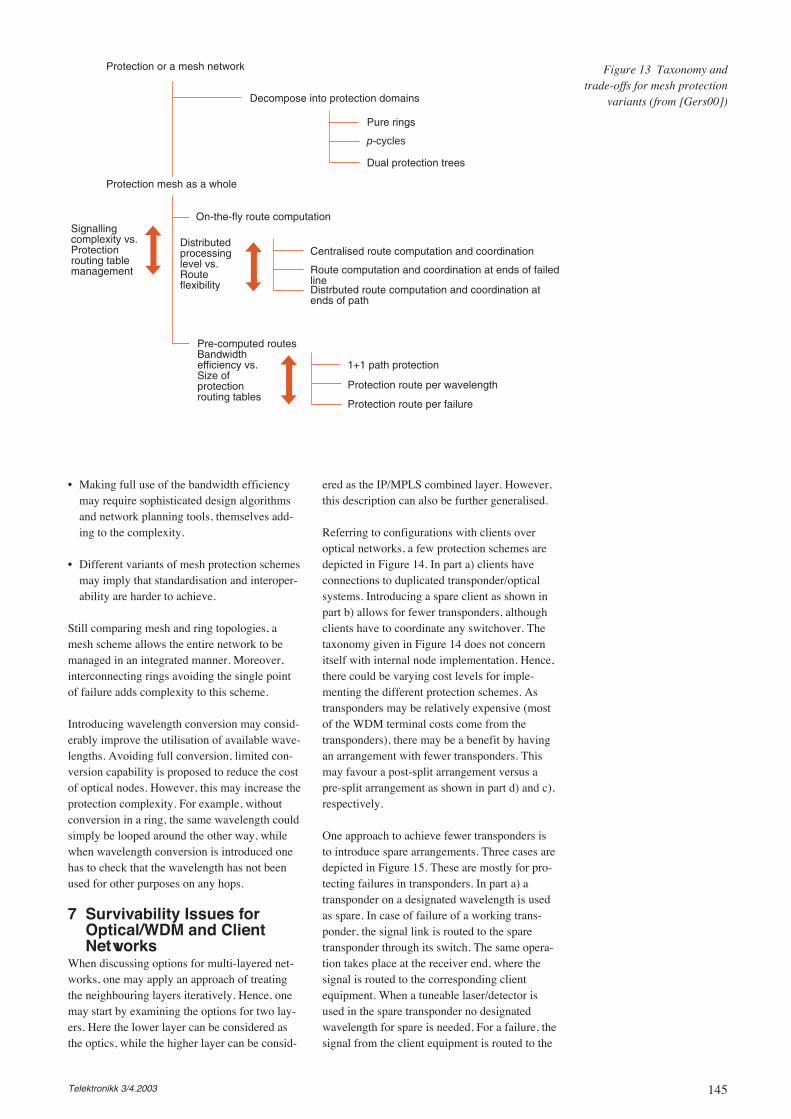
145Telektronikk 3/4.2003
• Making full use of the bandwidth efficiencymay require sophisticated design algorithmsand network planning tools, themselves add-ing to the complexity.
• Different variants of mesh protection schemesmay imply that standardisation and interoper-ability are harder to achieve.
Still comparing mesh and ring topologies, amesh scheme allows the entire network to bemanaged in an integrated manner. Moreover,interconnecting rings avoiding the single pointof failure adds complexity to this scheme.
Introducing wavelength conversion may consid-erably improve the utilisation of available wave-lengths. Avoiding full conversion, limited con-version capability is proposed to reduce the costof optical nodes. However, this may increase theprotection complexity. For example, withoutconversion in a ring, the same wavelength couldsimply be looped around the other way, whilewhen wavelength conversion is introduced onehas to check that the wavelength has not beenused for other purposes on any hops.
7 Survivability Issues forOptical/WDM and ClientNetworks
When discussing options for multi-layered net-works, one may apply an approach of treatingthe neighbouring layers iteratively. Hence, onemay start by examining the options for two lay-ers. Here the lower layer can be considered asthe optics, while the higher layer can be consid-
ered as the IP/MPLS combined layer. However,this description can also be further generalised.
Referring to configurations with clients overoptical networks, a few protection schemes aredepicted in Figure 14. In part a) clients haveconnections to duplicated transponder/opticalsystems. Introducing a spare client as shown inpart b) allows for fewer transponders, althoughclients have to coordinate any switchover. Thetaxonomy given in Figure 14 does not concernitself with internal node implementation. Hence,there could be varying cost levels for imple-menting the different protection schemes. Astransponders may be relatively expensive (mostof the WDM terminal costs come from thetransponders), there may be a benefit by havingan arrangement with fewer transponders. Thismay favour a post-split arrangement versus apre-split arrangement as shown in part d) and c),respectively.
One approach to achieve fewer transponders isto introduce spare arrangements. Three cases aredepicted in Figure 15. These are mostly for pro-tecting failures in transponders. In part a) atransponder on a designated wavelength is usedas spare. In case of failure of a working trans-ponder, the signal link is routed to the sparetransponder through its switch. The same opera-tion takes place at the receiver end, where thesignal is routed to the corresponding clientequipment. When a tuneable laser/detector isused in the spare transponder no designatedwavelength for spare is needed. For a failure, thesignal from the client equipment is routed to the
Protection or a mesh network
Decompose into protection domains
Pure rings
Dual protection trees
On-the-fly route computationSignallingcomplexity vs.Protectionrouting tablemanagement
Distributedprocessinglevel vs.Routeflexibility
Centralised route computation and coordination
Route computation and coordination at ends of failedlineDistrbuted route computation and coordination atends of path
Pre-computed routesBandwidthefficiency vs.Size ofprotectionrouting tables
1+1 path protection
Protection route per wavelength
Protection route per failure
Protection mesh as a whole
p-cycles
Figure 13 Taxonomy andtrade-offs for mesh protection
variants (from [Gers00])
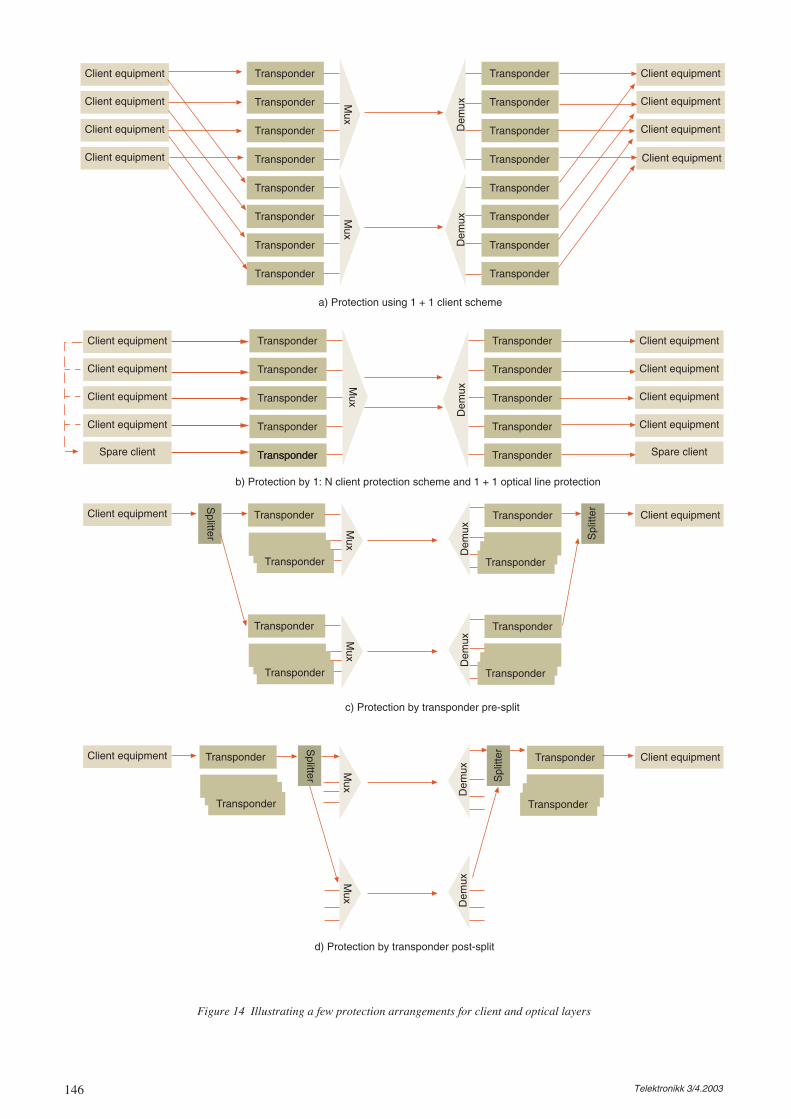
146 Telektronikk 3/4.2003
Figure 14 Illustrating a few protection arrangements for client and optical layers
Client equipment
Client equipment
Client equipment
Client equipment
Transponder
Transponder
Transponder
Transponder
Transponder
Transponder
Transponder
Transponder
Mux
Mux
Transponder
Transponder
Transponder
Transponder
Transponder
Transponder
Transponder
Transponder
Dem
uxD
emux
Client equipment
Client equipment
Client equipment
Client equipment
a) Protection using 1 + 1 client scheme
Client equipment
Client equipment
Client equipment
Client equipment
Transponder
Transponder
Transponder
Transponder
Transponder
Mux
Transponder
Transponder
Transponder
Transponder
TransponderD
emux
Client equipment
Client equipment
Client equipment
Client equipment
b) Protection by 1: N client protection scheme and 1 + 1 optical line protection
Spare client Spare client
c) Protection by transponder pre-split
Transponder
Transponder
Transponder
Client equipment
Splitter
Mux
Dem
ux
Transponder
Transponder
Client equipment
Spl
itter
Transponder
Transponder
Mux
Dem
ux
Transponder
Transponder
d) Protection by transponder post-split
Transponder
Transponder
Client equipment
Splitter
Mux
Dem
ux
Transponder
Transponder
Client equipment
Spl
itter
Mux
Dem
ux
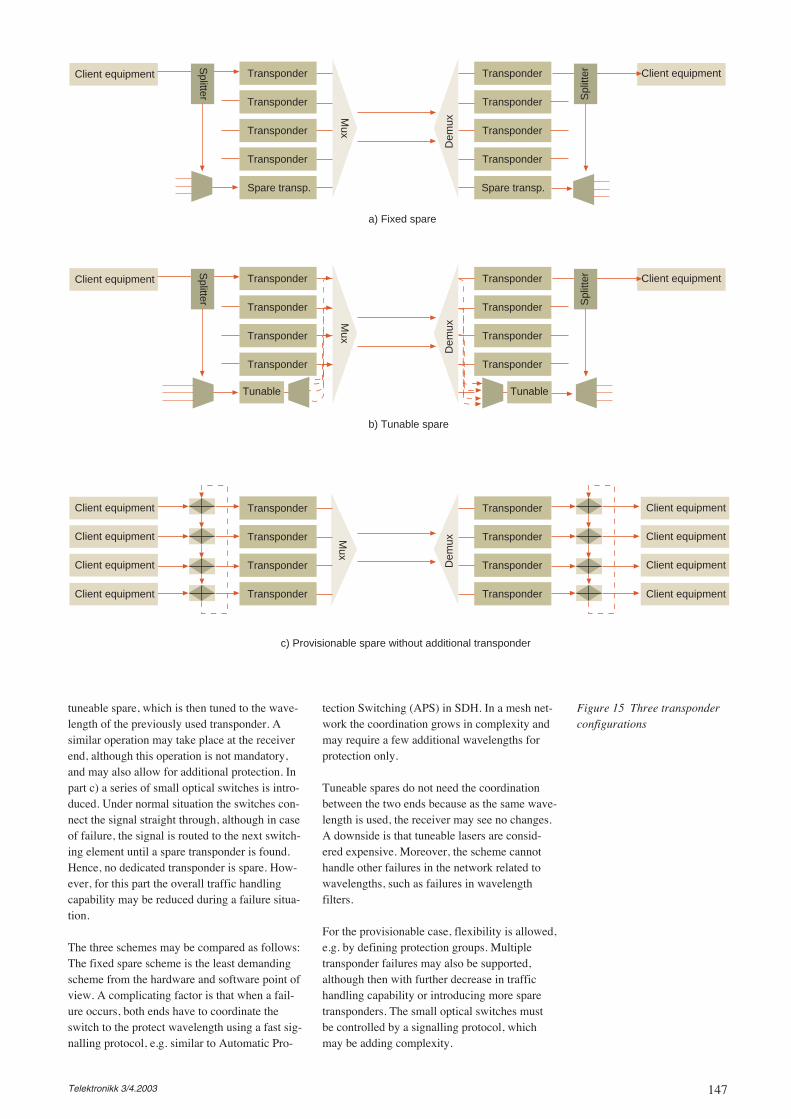
147Telektronikk 3/4.2003
Figure 15 Three transponderconfigurations
Client equipment Transponder
Transponder
Transponder
Transponder
Spare transp.
Mux
Transponder
Transponder
Transponder
Transponder
Dem
ux
Client equipment
a) Fixed spare
Splitter S
plitt
er
Client equipment Transponder
Transponder
Transponder
Transponder
Tunable
Mux
Transponder
Transponder
Transponder
Transponder
Dem
ux
Client equipment
b) Tunable spare
Splitter S
plitt
er
Spare transp.
Tunable
Client equipment Transponder
Transponder
Transponder
Transponder
Mux
Transponder
Transponder
Transponder
Transponder
Dem
ux
c) Provisionable spare without additional transponder
Client equipment
Client equipment
Client equipment
Client equipment
Client equipment
Client equipment
Client equipment
tuneable spare, which is then tuned to the wave-length of the previously used transponder. Asimilar operation may take place at the receiverend, although this operation is not mandatory,and may also allow for additional protection. Inpart c) a series of small optical switches is intro-duced. Under normal situation the switches con-nect the signal straight through, although in caseof failure, the signal is routed to the next switch-ing element until a spare transponder is found.Hence, no dedicated transponder is spare. How-ever, for this part the overall traffic handlingcapability may be reduced during a failure situa-tion.
The three schemes may be compared as follows:The fixed spare scheme is the least demandingscheme from the hardware and software point ofview. A complicating factor is that when a fail-ure occurs, both ends have to coordinate theswitch to the protect wavelength using a fast sig-nalling protocol, e.g. similar to Automatic Pro-
tection Switching (APS) in SDH. In a mesh net-work the coordination grows in complexity andmay require a few additional wavelengths forprotection only.
Tuneable spares do not need the coordinationbetween the two ends because as the same wave-length is used, the receiver may see no changes.A downside is that tuneable lasers are consid-ered expensive. Moreover, the scheme cannothandle other failures in the network related towavelengths, such as failures in wavelengthfilters.
For the provisionable case, flexibility is allowed,e.g. by defining protection groups. Multipletransponder failures may also be supported,although then with further decrease in traffichandling capability or introducing more sparetransponders. The small optical switches mustbe controlled by a signalling protocol, whichmay be adding complexity.
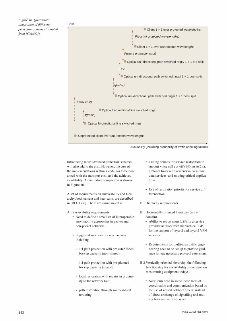
148 Telektronikk 3/4.2003
Introducing more advanced protection schemeswill also add to the cost. However, the cost ofthe implementations within a node has to be bal-anced with the transport cost, and the achievedavailability. A qualitative comparison is shownin Figure 16.
A set of requirements on survivability and hier-archy, both current and near-term, are describedin [RFC3386]. These are summarised as:
A. Survivability requirements:• Need to define a small set of interoperable
survivability approaches in packet andnon-packet networks
• Suggested survivability mechanismsincluding
- 1:1 path protection with pre-establishedbackup capacity (non-shared)
- 1:1 path protection with pre-plannedbackup capacity (shared)
- local restoration with repairs in proxim-ity to the network fault
- path restoration through source-basedrerouting
• Timing bounds for service restoration tosupport voice call cut-off (140 ms to 2 s),protocol timer requirements in premiumdata services, and missing critical applica-tions
• Use of restoration priority for service dif-ferentiation
B. Hierarchy requirements
B.1 Horizontally oriented hierarchy (intra-domain)• Ability to set up many LSPs in a service
provider network with hierarchical IGP,for the support of layer 2 and layer 2 VPNservices
• Requirements for multi-area traffic engi-neering need to be set up to provide guid-ance for any necessary protocol extensions.
B.2 Vertically oriented hierarchy; the followingfunctionality for survivability is common onmost routing equipment today:
• Near-term need in some loose form ofcoordination and communication based onthe use of nested hold-off timers, insteadof direct exchange of signalling and rout-ing between vertical layers
Figure 16 Qualitativeillustration of differentprotection schemes (adaptedfrom [Gers00])
Client 1 + 1 over protected wavelengths
F(cost of protected wavelengths)
Client 1 + 1 over unprotected wavelengths
F(client protection cost)
Optical uni-directional path switched rings/ 1 + 1 pre-split
x 2
Optical uni-directional path switched rings/ 1 + 1 post-split
Optical uni-directional path switched rings/ 1 + 1 post-split
f(traffic)
Optical bi-directional line switched rings
f(traffic)
Optical bi-directional line switched rings
Unprotected client over unprotected wavelengths
Cost
Availability (including probability of traffic affecting failure)
f(mux cost)
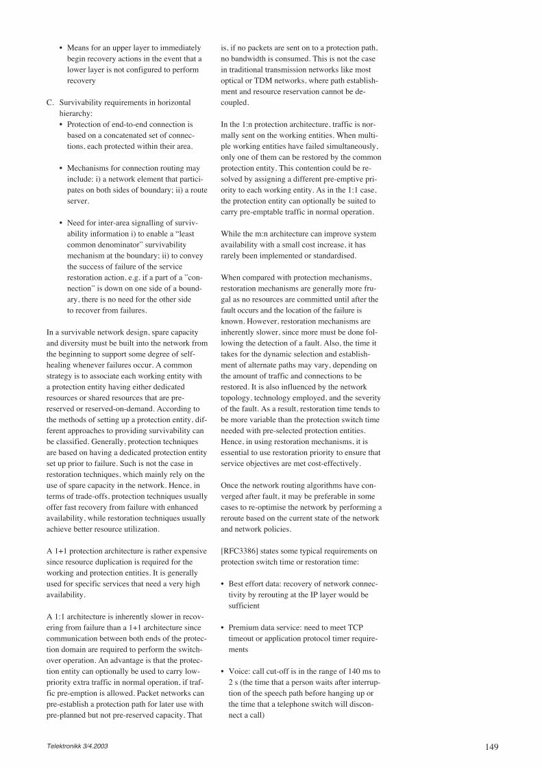
149Telektronikk 3/4.2003
• Means for an upper layer to immediatelybegin recovery actions in the event that alower layer is not configured to performrecovery
C. Survivability requirements in horizontalhierarchy:• Protection of end-to-end connection is
based on a concatenated set of connec-tions, each protected within their area.
• Mechanisms for connection routing mayinclude: i) a network element that partici-pates on both sides of boundary; ii) a routeserver.
• Need for inter-area signalling of surviv-ability information i) to enable a “leastcommon denominator” survivabilitymechanism at the boundary; ii) to conveythe success of failure of the servicerestoration action, e.g. if a part of a ”con-nection” is down on one side of a bound-ary, there is no need for the other sideto recover from failures.
In a survivable network design, spare capacityand diversity must be built into the network fromthe beginning to support some degree of self-healing whenever failures occur. A commonstrategy is to associate each working entity witha protection entity having either dedicatedresources or shared resources that are pre-reserved or reserved-on-demand. According tothe methods of setting up a protection entity, dif-ferent approaches to providing survivability canbe classified. Generally, protection techniquesare based on having a dedicated protection entityset up prior to failure. Such is not the case inrestoration techniques, which mainly rely on theuse of spare capacity in the network. Hence, interms of trade-offs, protection techniques usuallyoffer fast recovery from failure with enhancedavailability, while restoration techniques usuallyachieve better resource utilization.
A 1+1 protection architecture is rather expensivesince resource duplication is required for theworking and protection entities. It is generallyused for specific services that need a very highavailability.
A 1:1 architecture is inherently slower in recov-ering from failure than a 1+1 architecture sincecommunication between both ends of the protec-tion domain are required to perform the switch-over operation. An advantage is that the protec-tion entity can optionally be used to carry low-priority extra traffic in normal operation, if traf-fic pre-emption is allowed. Packet networks canpre-establish a protection path for later use withpre-planned but not pre-reserved capacity. That
is, if no packets are sent on to a protection path,no bandwidth is consumed. This is not the casein traditional transmission networks like mostoptical or TDM networks, where path establish-ment and resource reservation cannot be de-coupled.
In the 1:n protection architecture, traffic is nor-mally sent on the working entities. When multi-ple working entities have failed simultaneously,only one of them can be restored by the commonprotection entity. This contention could be re-solved by assigning a different pre-emptive pri-ority to each working entity. As in the 1:1 case,the protection entity can optionally be suited tocarry pre-emptable traffic in normal operation.
While the m:n architecture can improve systemavailability with a small cost increase, it hasrarely been implemented or standardised.
When compared with protection mechanisms,restoration mechanisms are generally more fru-gal as no resources are committed until after thefault occurs and the location of the failure isknown. However, restoration mechanisms areinherently slower, since more must be done fol-lowing the detection of a fault. Also, the time ittakes for the dynamic selection and establish-ment of alternate paths may vary, depending onthe amount of traffic and connections to berestored. It is also influenced by the networktopology, technology employed, and the severityof the fault. As a result, restoration time tends tobe more variable than the protection switch timeneeded with pre-selected protection entities.Hence, in using restoration mechanisms, it isessential to use restoration priority to ensure thatservice objectives are met cost-effectively.
Once the network routing algorithms have con-verged after fault, it may be preferable in somecases to re-optimise the network by performing areroute based on the current state of the networkand network policies.
[RFC3386] states some typical requirements onprotection switch time or restoration time:
• Best effort data: recovery of network connec-tivity by rerouting at the IP layer would besufficient
• Premium data service: need to meet TCPtimeout or application protocol timer require-ments
• Voice: call cut-off is in the range of 140 ms to2 s (the time that a person waits after interrup-tion of the speech path before hanging up orthe time that a telephone switch will discon-nect a call)
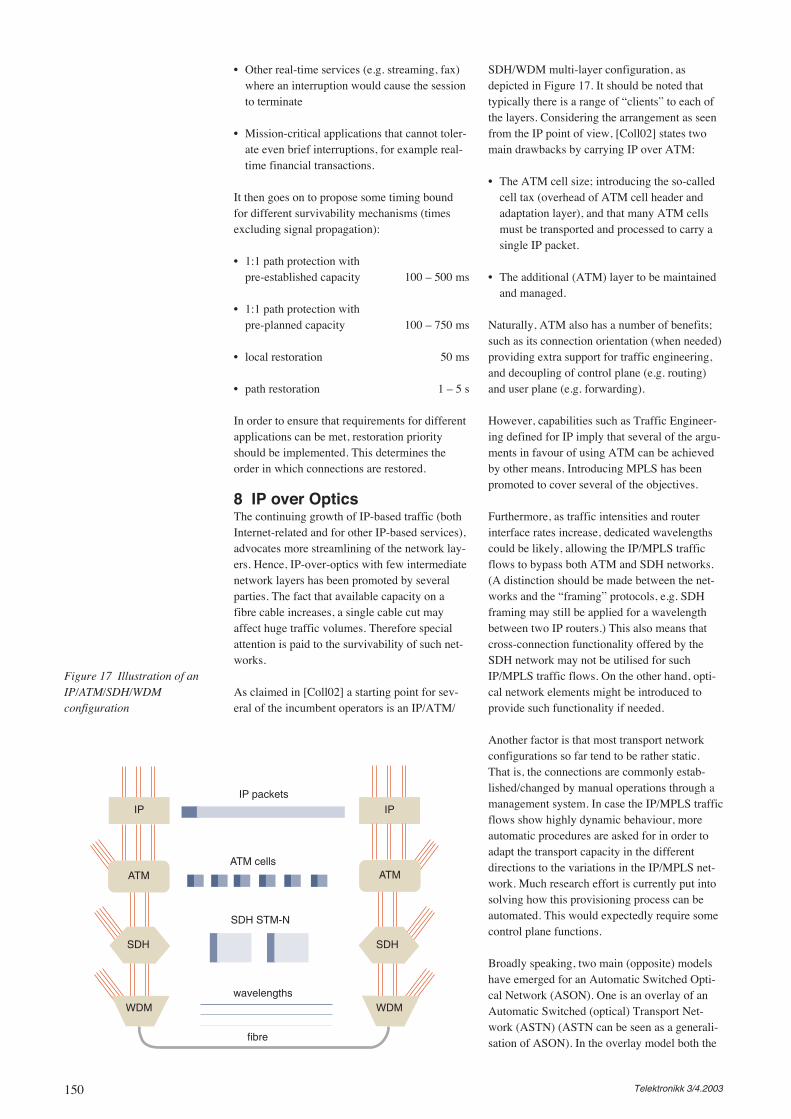
150 Telektronikk 3/4.2003
• Other real-time services (e.g. streaming, fax)where an interruption would cause the sessionto terminate
• Mission-critical applications that cannot toler-ate even brief interruptions, for example real-time financial transactions.
It then goes on to propose some timing boundfor different survivability mechanisms (timesexcluding signal propagation):
• 1:1 path protection with pre-established capacity 100 – 500 ms
• 1:1 path protection with pre-planned capacity 100 – 750 ms
• local restoration 50 ms
• path restoration 1 – 5 s
In order to ensure that requirements for differentapplications can be met, restoration priorityshould be implemented. This determines theorder in which connections are restored.
8 IP over OpticsThe continuing growth of IP-based traffic (bothInternet-related and for other IP-based services),advocates more streamlining of the network lay-ers. Hence, IP-over-optics with few intermediatenetwork layers has been promoted by severalparties. The fact that available capacity on afibre cable increases, a single cable cut mayaffect huge traffic volumes. Therefore specialattention is paid to the survivability of such net-works.
As claimed in [Coll02] a starting point for sev-eral of the incumbent operators is an IP/ATM/
SDH/WDM multi-layer configuration, asdepicted in Figure 17. It should be noted thattypically there is a range of “clients” to each ofthe layers. Considering the arrangement as seenfrom the IP point of view, [Coll02] states twomain drawbacks by carrying IP over ATM:
• The ATM cell size; introducing the so-calledcell tax (overhead of ATM cell header andadaptation layer), and that many ATM cellsmust be transported and processed to carry asingle IP packet.
• The additional (ATM) layer to be maintainedand managed.
Naturally, ATM also has a number of benefits;such as its connection orientation (when needed)providing extra support for traffic engineering,and decoupling of control plane (e.g. routing)and user plane (e.g. forwarding).
However, capabilities such as Traffic Engineer-ing defined for IP imply that several of the argu-ments in favour of using ATM can be achievedby other means. Introducing MPLS has beenpromoted to cover several of the objectives.
Furthermore, as traffic intensities and routerinterface rates increase, dedicated wavelengthscould be likely, allowing the IP/MPLS trafficflows to bypass both ATM and SDH networks.(A distinction should be made between the net-works and the “framing” protocols, e.g. SDHframing may still be applied for a wavelengthbetween two IP routers.) This also means thatcross-connection functionality offered by theSDH network may not be utilised for suchIP/MPLS traffic flows. On the other hand, opti-cal network elements might be introduced toprovide such functionality if needed.
Another factor is that most transport networkconfigurations so far tend to be rather static.That is, the connections are commonly estab-lished/changed by manual operations through amanagement system. In case the IP/MPLS trafficflows show highly dynamic behaviour, moreautomatic procedures are asked for in order toadapt the transport capacity in the differentdirections to the variations in the IP/MPLS net-work. Much research effort is currently put intosolving how this provisioning process can beautomated. This would expectedly require somecontrol plane functions.
Broadly speaking, two main (opposite) modelshave emerged for an Automatic Switched Opti-cal Network (ASON). One is an overlay of anAutomatic Switched (optical) Transport Net-work (ASTN) (ASTN can be seen as a generali-sation of ASON). In the overlay model both the
Figure 17 Illustration of anIP/ATM/SDH/WDMconfiguration
IP IP
ATM ATM
SDH
WDM
SDH
WDM
IP packets
ATM cells
SDH STM-N
wavelengths
fibre
151Telektronikk 3/4.2003
transport network and its client networks have aseparated and independent control plane. This isdescribed in ITU-T recommendations.
The IETF seems to target a peer model with theGeneralised MPLS (GMPLS) concept. This con-cept stems from MPλS, where the underlyingidea was that a wavelength is a “label” like anyother layer and therefore the MPLS concept canbe adopted in the optical domain to serve theneed for fast and automatic provisioning ofwavelengths. GMPLS is more generic in thesense that it considers any type of label: a headerstring for packet switch capable LSR (PSC-LSR), a time slot for a TDM switch capable LSR(TSC-LSR, e.g. by SDH), a wavelength for alambda-switch capable LSR (LSC-LSR, e.g. anoptical cross-connect), or a fibre in a fibre-switch capable LSR (FSC-LSR). These aredescribed in Section 3.2.
Although both client and transport networksmay have their own separate and independent(G)MPLS control planes, an integration of thesecontrols planes into a singe one seems tempting.This then results in the so-called peer model.The following advantages are seen for the peermodel:
• Avoiding duplication of control plane func-tionality in distinct layers;
• Avoiding the requirements of standardisationof a User-Network Interface betweenIP/MPLS routers and optical network compo-nents.
A basic drawback, however, is the fact that inte-gration and compatibility among multiple clienttype networks seem hard, as well as the require-ment that all necessary information of the opticalnetwork (e.g. the topology) will be accessible inthe client domain.
9 All Protection at IP LayerSome people claim there is a trend that most ofthe protection is located at the IP/MPLS layer.This is backed by arguments such as:
• Protection at SDH is considered as expensiveas seen by the IP/MPLS layer (one pays for aback-up capacity that is rarely used).
• Supporting differentiated protection schemesimplies that such mechanisms must be locatedat the IP/MPLS layer.
• Several people would remove the SDH net-work as such for carrying the IP/MPLS traffic(although SDH framing may still be applied).
A consequence of this is that links between IProuters should be disjoint in order to handle fail-ures. In this perspective, one can consider the IPnetwork as consisting of a set of logical linksthat are mapped onto a set of physical links inthe fibre/WDM network. In the WDM networkthe logical links are assigned a wavelength, orpossibly a sequence of wavelengths if wave-length conversion is present. In this way severallogical links could go on the same fibre (or con-duit), which is not a preferred situation as a sin-gle cable cut could affect several links.
When a failure occurs in the optical equipment,one should still have a connected topology at theIP layer. Hence, for every possible failure, alter-native operational logical links (or combinationsof logical links) must exist so that alternativeroutes can be found by the IP routing protocol.
A requirement may then be that the alternativelink offers about the same delay as the normaloperating link. For example, a voice-over-IPapplication may suffer if the end-to-end delayincreases by more than 50 ms after switchingover to the alternative link. This comes in addi-tion to the fact that the primary operating linkusually follows the shortest path and thereby hasthe shortest delay.
Hence, designing the robust IP network, bothdisjoint links as well as delay concerns have tobe included. The latter would naturally berelated to the link loads. Having two differenttypes of requirements commonly asks for atrade-off (or combination) to be included. Thebasic problem can be formulated as an IntegerProgramming problem (integer refers to the factthat one must choose from certain capacities andthat logical links must be mapped onto physicallinks). Generally this is known as an NP-com-plete problem, where delay constraints, limitednumber of wavelengths and fibre/WDM networkstructure have to be considered.
10 MPLS-Based ProtectionSeveral of today’s networks are firstly built forconnectivity, and secondly to support one ser-vice class. The migration of real-time andhigher-priority traffic to IP networks means thatmodern IP networks increasingly carry mission-critical business data and must therefore providereliable transmission. Current routing algo-rithms, despite being robust and survivable, cantake a substantial amount of time to recoverfrom a failure, which can be in the order of sev-eral seconds to minutes and can cause seriousdisruption of service in the interim. This is unac-ceptable for many applications that require ahighly reliable service, and has motivated net-work providers to give serious consideration tothe issues of network survivability.
152 Telektronikk 3/4.2003
Multi Protocol Label Switching (MPLS) canbe utilised to integrate forwarding based onlabel-swapping of a local label and hence allowsmore advanced forwarding mechanisms to beapplied. One area of these mechanisms is QoS,where MPLS can be used to transport data reli-ably and efficiently and also to support a rangeof service classes. One of the drawbacks withcurrent IP routing algorithms is the relativelylong time to recover from a fault, which is inthe order of seconds or minutes. This may wellcause a disruption of service as observed by theapplications/users. As more business-criticalapplications/usages and real-time demandingapplications are placed on IP networks, suchlong recovery times may be unacceptable. It isoften seen that applications require recoverytimes down to tens of milliseconds; examplesbeing virtual leased lines, voice traffic, realvideo transfers, stock exchange data. For severalof these applications SLA conditions have beenstated which do not allow for long recoverytimes.
Generally, operators would provide the fastestand best protection mechanisms that can be pro-vided at a reasonable cost. However, the higherlevel of protection, the more resources con-sumed. Hence, it is naturally expected that oper-ators will offer a range of service levels. MPLS-based recovery should give the flexibility toselect the recovery mechanism, choose the gran-ularity of which traffic to protect and also tochoose the specific types of traffic that are pro-tected in order to give operators more controlover that trade-off.
Based on the above, one motivation for MPLS isthe notion that the current IP routing algorithmshave limited potential for improving the recov-ery times. Introducing recovery mechanisms onthe MPLS level, or partly enhance the currentrouting algorithms with MPLS aspects may alle-viate the underlying restriction.
Another motivation for introducing recoverymechanisms operating on the MPLS level is thepresence of MPLS in several of the IP networks.Moreover, MPLS is commonly promoted as abase solution for IP-based transport networks.Hence, it is natural that MPLS provides protec-tion and restoration of the traffic that has suchrequirements.
MPLS may facilitate the convergence of net-work functionality on a common control andmanagement plane. Further, a protection prioritycould be used as a differentiating mechanism forpremium services that require high reliability.
TermsThe intent of protection is to protect against anylink or node fault on a path or a segment of apath. The protected path is commonly referred toas a working path. A set of paths used for carry-ing traffic on the working path in case of failurealong it, is commonly referred to as recoverypaths. An LSR that can select to use the workingpath or the recovery path is called a Path SwitchLSR (PSL). The LSR where the working andrecovery paths meet has to decide which packetsthat should be forwarded. This LSR is com-monly called a Path Merge LSR (PML).
As LSPs are unidirectional and recovery maywell require notification of faults being carriedto the LSR responsible for switch-over to therecovery path, a mechanism must be providedfor propagating fault and repair indications fromthe point of occurrence of the fault back to thatLSR. These are called Fault Indication Signal(FIS) and Fault Repair Signal (FRS).
10.1 Recovery PrinciplesA nomenclature for recovery principles is alsodrafted in [Shar02]. Firstly it is noted that MPLS-based recovery refers to the ability to quicklyand completely restore capabilities for servingtraffic affected by a fault in an MPLS network.The fault may be detected at the IP layer or inlower layers. To some extent the different termscan be arranged in a “nomenclature tree” asdepicted in Figure 18.
The issues and corresponding options are:
1. Configuration of recovery:• Default recovery: no MPLS-based re-
covery is enabled; hence traffic must berecovered using IP layer or lower layermechanisms.
• Recoverable: MPLS-based recovery isenabled; hence one or more MPLS re-covery paths are identified for a workingMPLS path.
2. Initiation of path set-up:• Pre-established: recovery paths are estab-
lished prior to any failure of the workingpath. This is also called protectionswitching.
• Pre-qualified: a path created for otherpurposes is also designated as a recoverypath for a working path.
• Established on-demand: a recovery pathis established after a failure on its work-ing path has been detected and notifiedto the Path Switched LSR (PSL). This isalso called re-routing option.
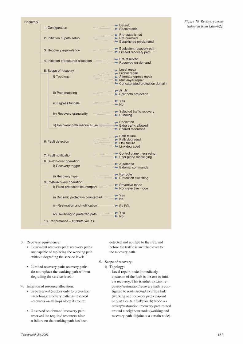
153Telektronikk 3/4.2003
Recovery
1. Configuration
2. Initiation of path setup
3. Recovery equivalence
4. Initiation of resource allocation
5. Scope of recovery
i) Topology
ii) Path mapping
iii) Bypass tunnels
iv) Recovery granularity
v) Recovery path resource use
6. Fault detection
7. Fault notification
8. Switch-over operationi) Recovery trigger
ii) Recovery type
9. Post-recovery operationi) Fixed protection counterpart
ii) Dynamic protection counterpart
iii) Restoration and notification
iv) Reverting to preferred path
10. Performance – attribute values
DefaultRecoverable
Pre-establishedPre-qualifiedEstablished on-demand
Equivalent recovery pathLimited recovery path
Pre-reservedReserved on-demand
Local repairGlobal repairAlternate egress repairMulti-layer repairConcatenated protection domain
N : MSplit path protection
YesNo
Selected traffic recoveryBundling
DedicatedExtra traffic allowedShared resources
Path failurePath degradedLink failureLink degraded
Control plane messagingUser plane messaging
AutomaticExternal commands
Re-routeProtection switching
Revertive modeNon-revertive mode
YesNo
By PSL
YesNo
Figure 18 Recovery terms(adapted from [Shar02])
3. Recovery equivalence:• Equivalent recovery path: recovery paths
are capable of replacing the working pathwithout degrading the service levels.
• Limited recovery path: recovery pathsdo not replace the working path withoutdegrading the service levels.
4. Initiation of resource allocation:• Pre-reserved (applies only to protection
switching): recovery path has reservedresources on all hops along its route.
• Reserved on-demand: recovery pathreserved the required resources aftera failure on the working path has been
detected and notified to the PSL andbefore the traffic is switched over tothe recovery path.
5. Scope of recovery:i) Topology:
- Local repair: node immediatelyupstream of the fault is the one to initi-ate recovery. This is either a) Link re-covery/restoration/recovery path is con-figured to route around a certain link(working and recovery paths disjointonly at a certain link); or, b) Node re-covery/restoration: recovery path routedaround a neighbour node (working andrecovery path disjoint at a certain node).

154 Telektronikk 3/4.2003
- Global repair: Point Of Repair (POR) isat the ingress of a path (segment), hencealso covering end-to-end path recovery.In case the recovery path is completelydisjoint from the working path, this pro-tects against any link and node faults.
- Alternate egress repair: the recoverypath may have a different egress pointfrom the working path.
- Multi-layer repair: several networklayers are managed together in order toachieve adequate protection of the traf-fic flows (ref. Chapter 5).
- Concatenated protection domains: re-covery provided for traffic flows cross-ing a number of network domains. Asthese domains may apply differentrecovery mechanisms it is still impor-tant that the end-to-end protection isadequate.
ii) Path mapping (mapping of traffic fromworking path to set of recovering paths):- N:M protection: up to N working paths
are protected using M recovery paths.Common configurations are 1:1 and N:1protection.
- Split path protection: multiple recoverypaths carry the traffic of a working pathaccording to configurable splittingratios. Typically, this is used when nosingle recovery paths can carry theentire traffic load of the working path.This may require the Path Merge LSR,PML(s) to correlate the traffic arrivingon multiple recovery paths with theworking path. In principle a 1+1 config-uration could be seen as a special casewhere the traffic is carried on two pathsbetween the PSL and PML, and thePML correlates the packets arrivingalong the two paths.
iii)Bypass tunnels: creation of a tunnel(MPLS path) for a Path Protection Group(PPG) between a PSL and PML. Thenone MPLS path – the tunnel – carries anumber of paths by label stacking, there-by making all the “inner paths” transpar-ent to intermediate LSRs.
iv) Recover granularity (refers to the ratio oftraffic requiring protection (e.g. rangingfrom a fraction of a path to a bundle ofpaths):- Selective traffic recovery: protection
of a fraction of traffic within the same
path, referred to a protection traffic por-tion (PTP).
- Bundling: grouping several workingpaths allowing for simultaneous recov-ery. The logical bundling of these work-ing paths routing between the same PSLand PML is called a Protected PathGroup (PPG). When a fault occurs onthe working path carrying the PPG, thePPG as a whole can be protected.
v) Recovery path resource use (referring tooptional use of pre-reserved recoverypaths when that path is not in use – nofault on the working path):- Dedicated resource: the recovery path
resources may not be used by other traf-fic flows.
- Extra traffic allowed: the recovery pathmay carry other traffic flows when thatcapacity is not needed by traffic on theworking path, e.g. when there is no faulton the working path. Extra traffic can bedisplaced whenever the recovery pathresources are needed to carry the work-ing path traffic.
- Shared resource: recovery path re-sources are used by several workingpaths (where all of the working pathsare not assumed to fail simultaneously).
6. Fault detection• Path Failure (PF): an indication to the
MPLS mechanisms that the connectivityof the path is lost. This could, for exam-ple, be identified by path continuity testor liveness messages/probes.
• Path Degraded (PD): an indication to theMPLS mechanisms that the service levelon the path is unacceptable. This maytypically be done local to an LSR, e.g. byreceiving many packets with incorrectlabels or TTL.
• Link Failure (LF): an indication from alower layer to MPLS recovery mecha-nisms that the link has failed. This mayfor example be Loss Of Signal (LOS)from SDH.
• Link Degraded (LD): an indication froma lower layer to MPLS recovery mecha-nisms that the link gives an unacceptableservice level.
7. Fault notification (when a fault is severeenough to require path recovery, an inform-ed node must take appropriate actions. In

155Telektronikk 3/4.2003
case the node is not capable of initiateddirect actions, notification of the faultsshould be sent to the POR):• Notification by control plane messaging:
relaying hop-by-hop along the path untila POR is reached.
• Notification by user plane messaging:typically sent downstream to the PMLwhich then takes corrective action (e.g. asPOR for 1+1) or communicate with aPOR (by control plane messaging or userplane messaging for a bi-directionalLSP).
8. Switch-over operation:i) Recovery trigger: MPLS protection
switching may be initiated because ofautomatic inputs of external commands.Automatic inputs include fault notifica-tions received (when several notificationsare received for the same fault case, theseshould be correlated).
ii) Recovery action: a POR executes therecovery actions, either re-routing or pro-tection switching as described earlier.
9. Post-recovery operation (refers to decisionsmade after traffic flows on the recovery path):i) Fixed protection counterparts:
- Revertive mode: when the fault on the(original) working path is cleared, thetraffic is switched back to this path,from the (original) recovery path.
- Non-revertive mode: a switch back tothe (original) working path is not imme-diately carried out even after the faulthas been cleared. When the fault in the(original) working path is cleared, thatpath may be used for other purposes, orbe defined as a recovery path for the onewhere traffic has been switched on to.
ii) Dynamic protection counterparts: whenthe network reaches a stable state after thefault, traffic on the recovery path may beswitched over to a different preferred path(not the original working path).
iii)Restoration and notification: reversion isperformed by the PSL by receiving notifi-cation that the working path is repaired orthat a new working path is established.
iv) Reverting to preferred path (or controlledrearrangement): typically this involves a“make before break” switching.
10. Performance: the recovery paths will typi-cally have a number of attributes, including
i) resource class attributes (in case of equiva-lence these are the same as the workingpath), ii) path priority attributes, iii) pathpre-emption attributes.
When several MPLS-based recovery schemesare compared, a set of criteria has to be defined.[Shar02] proposes the following criteria:
• Recovery time: this time can be defined as theinterval from the fault occurred until a recov-ery path is carrying the relevant traffic. Hence,it is the sum of the fault detection time, hold-off time, notification time, recovery operationtime and traffic restoration time.
• Full restoration time: this time is defined asthe interval from the fault occurred until a per-manent restoration is reached. A permanentrestoration reflects the state when traffic flowson links capable of or having been engineeredto handle traffic as expected. This time maydiffer from the recovery time depending onwhen limited recovery paths are used (asopposed to equivalent paths).
• Set up vulnerability: the amount of time a setof working paths is left unprotected duringrecovery (such as path computation and set-up).
• Back-up capacity: capacity needed duringrecovery (also depending on traffic character-istics as well as protection plan selection algo-rithms and signalling and re-routing methods.
• Additive latency: additional delays along therecovery path compared with the workingpath.
• Quality of protection: includes relative andabsolute survivability. Relative means that thetraffic flow in question has the same serviceclass as other flows (contending for the sameresources). Absolute means that explicit guar-antees may be given to the protected traffic.
• Re-ordering: packets may arrive in a differentorder than sent during recovery (the same mayhappen during restoration)
• State overhead: the amount of informationneeded to maintain the paths
• Loss: a certain amount of packet loss may beintroduced during switch-overs.
• Coverage: representing various types of fail-overs: i) Fault types (link faults, node faults,degraded service level, etc.), ii) Number ofconcurrent faults, iii) Number of recoverypaths, iv) Percentage of coverage (certain per-centage of fault types), and v) Number of pro-
156 Telektronikk 3/4.2003
tected paths compared with the total numberof paths (e.g. given as n/N where n is the num-ber of protected paths and N is the total num-ber of paths).
10.2 MPLS Recovery ObjectivesAs stated in [Shar02], MPLS-based recovery ismotivated by a number of arguments:
• Ability to increase network availability by en-abling faster response to faults than possiblewith mechanisms only related to the IP layer.
• IP rerouting may often be too slow for a coreMPLS network that needs to support recoverytimes smaller than convergence times of IProuting protocols.
• Utilising lower layers (e.g. optical channels –sometimes referred to as layer 0, and SDH –sometimes referred to as layer 1) may result inwasteful use of resources. That is, the granu-larity of the resources may be too coarse forthe group of traffic flows that should be pro-tected.
• IP-traffic can be put directly over WDM chan-nels to provide recovery options without anintervening SDH layer (supports building IP-over-WDM networks). Commonly mecha-nisms on optical layer and SDH layer do nothave visibility into higher layer operations.Hence, they may provide e.g. link protectionby not easily providing node protection orprotection of traffic transported at the IP layer.Moreover, this may prevent the lower layersfrom providing restoration based on the needsof the traffic flows. An example is that fastrestoration could be provided only to trafficflows that need this, while slower restorationcould be used for traffic flows that do notneed fast restoration (slower restoration mayalso allow for time to find more optimal use ofthe resources). For cases where the latter traf-fic type is dominant, providing fast restorationto all traffic types may not be most effectivefrom an operator’s point of view.
MPLS Recovery Goals[Shar02] also states a number of goals forMPLS-based recovery. These may be broadlydivided into:
A. Resource-related:• Allow for better overall use of the network
resources, e.g. subject to traffic engineer-ing goals
• Maximise network reliability and avail-ability, e.g. by minimising number of sin-gle points of failure in the MPLS-pro-tected domain
• Recovery techniques may be applicablefor an entire end-to-end path or for seg-ments thereof.
• MPLS-based recovery mechanisms shouldtake into account recovery actions forlower layers. MPLS-based mechanismsshould not trigger lower layer protectionswitching.
• Minimise the state overhead incurred foreach recovery path maintained.
• Preserve the constraints on traffic afterswitch-over. That is, if desired, the recov-ery path should meet the resource require-ments of, and achieve the same perfor-mance characteristics as the working path.
B. Traffic-related:• Facilitate restoration times that are suffi-
ciently fast for the end-user application,i.e. matching the application’s require-ments.
• Enhance the reliability of the protectedtraffic while minimally or predictablydegrading the traffic carried by thediverted resources.
• Protection of traffic at various granulari-ties. For example to specify MPLS-basedrecovery for a portion of the traffic on anindividual path, for all traffic on an indi-vidual path, or for all traffic on a group ofpaths.
• Minimise loss of data and packet reorder-ing during recovery operations.
Several of these goals may be in conflict witheach other. Moreover, engineering compromiseswould be done based on a range of factors suchas cost, application requirements, network effi-ciency, and revenue considerations.
FeaturesFrom an operational point of view, [Shar02] liststhe following desirable features:
• MPLS recovery provides an option to identifyprotection groups (PPGs) and protection por-tions (PTPs).
• Each PSL is capable of performing MPLSrecovery upon detection of impairments orreceipt of notification of impairments.
• Manual protection switching commands arenot precluded.
157Telektronikk 3/4.2003
• A PSL is capable of performing a switch backto the original working path when the fault iscleared or a switch-over to a new working path.
• Path merging at intermediate LSRs must bepossible. If a fault affects the merged segmentall the paths sharing that merged segmentshould be able to recover. If a fault affectsa non-merged segment only the path that isaffected by the fault should be recovered.
10.3 Recovery and ProtectionSchemes
Basically, there are two models for path recov-ery: rerouting and protection switching. Recov-ery by rerouting is defined as establishing newpaths or path segments on demand for restoringtraffic after the occurrence of a fault. For protec-tion switching mechanisms a recovery path (orpath segment) is pre-established. The pre-estab-lished path may or may not be link and node dis-joint with the working path. If it is not disjoint,the overall reliability is degraded.
As traffic dynamics grows, requirements onnetwork survivability are not becoming morerelaxed. During recent years, much work andinterest have been attached to finding efficientways of allocating spare capacity in survivablenetworks. Several approaches still utilise NP-hardoptimisation process based on static working traf-fic demands [Ho02]. Most of the static schemescan be used for reallocating the spare capacitywhile the network is running. However, this ismostly after a time-consuming optimisation pro-cess. Hence the derived solution can be far fromoptimal as traffic rapidly changes. A conclusionin [Ho02] is that the static schemes are moresuited for use in designing small-sized networks,or networks where demands are less dynamic.
One attempt to overcome the computationalcomplexity is to introduce heuristic algorithms,introducing a compromise between performance(efficient resource utilisation) and computationalefficiency. [Ho02] names this process a surviv-able routing. A survivable routing algorithm isused to dynamically allocate the current connec-tion request into a network with protection ser-vice, while maximising the probability of suc-cessfully allocating subsequent connectionrequests in the network.
In contrast to dedicated protection such as 1+1,when a shared protection scheme is used, severalworking paths may use the same protectionresource. However, when two working pathsshare the same risk of failure (e.g. caused by thesame fault), they may not share the same protec-tion resources. Obeying this, it is possible toguarantee the level of impact that a single fault(link or node) would have.
Basically, two shared protection schemes are:
• Path-based: the source node of a working pathcomputes a protection path by ensuring thatthe protection path is diversely routed fromthe working path. If a fault occurs on theworking path, the terminating node in its con-trol plane detects the fault and sends a notifi-cation to the first node in the path to activate aswitch-over. The source node switches overthe traffic from the working path to the protec-tion path. As the path length influences therestoration time, a short failure recovery timemay be hard to reach.
• Link-based: fault localisation and restorationis done at upstream neighbour node of thefailed link or node and the traffic merged backto the original working path at the down-stream neighbour node. This may allow fastrestoration due to rapid fault localisation.
In addition to the short restoration times, fineservice granularity and high network throughputare sought.
Protection domains are commonly introduced.Subsequently, a diversely routed protection pathsegment is sought for each working path seg-ment within a protection domain. A domaindiameter may then be introduced, defined as theshortest path (hop count) between a source pathnode and termination path node. Referring tothis measure, link-based would have a diameterequal to one, while path-based would have adiameter equal to the working path length. Adja-cent protection domains must overlap in order toprotect against every single link/node failurealong the working path (e.g. the node on theedge of a domain), see Figure 19.
When a fault occurs on a working path, the firstnode in the protection domain where the faultoccurs is notified and activates a trafficswitchover. For example, a fault on link C – Dis detected by node D and signalled to node Athat switches the traffic to the protection path.A fault on link G – H is detected by node H andsignalled to node E that switches over the traffic.
As argued in [Ho02], introducing protectiondomains allows for shorter restoration times(only within a domain), less computationalcomplexity (needs to find restoration within thedomain only), and potentially higher resourceutilisation (protection paths could be shared out-side the domain). From a network managementperspective, it allows a trade-off between restor-ation time and amount of protection resourcesconsumed. A major drawback is the increase ofsignalling.
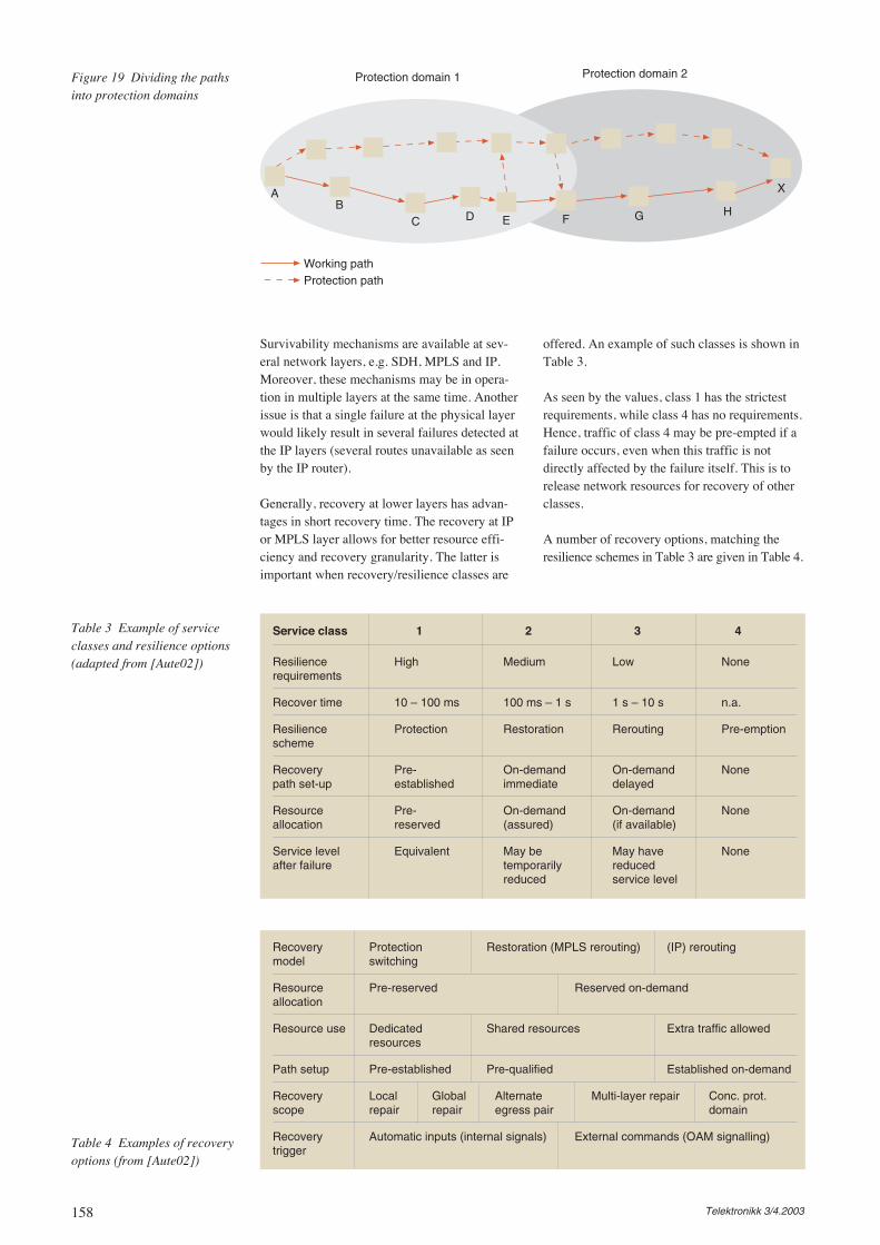
158 Telektronikk 3/4.2003
Survivability mechanisms are available at sev-eral network layers, e.g. SDH, MPLS and IP.Moreover, these mechanisms may be in opera-tion in multiple layers at the same time. Anotherissue is that a single failure at the physical layerwould likely result in several failures detected atthe IP layers (several routes unavailable as seenby the IP router).
Generally, recovery at lower layers has advan-tages in short recovery time. The recovery at IPor MPLS layer allows for better resource effi-ciency and recovery granularity. The latter isimportant when recovery/resilience classes are
offered. An example of such classes is shown inTable 3.
As seen by the values, class 1 has the strictestrequirements, while class 4 has no requirements.Hence, traffic of class 4 may be pre-empted if afailure occurs, even when this traffic is notdirectly affected by the failure itself. This is torelease network resources for recovery of otherclasses.
A number of recovery options, matching theresilience schemes in Table 3 are given in Table 4.
Protection domain 1 Protection domain 2
Working pathProtection path
AB
C D E F G H
X
Figure 19 Dividing the pathsinto protection domains
Service class 1 2 3 4
Resilience High Medium Low Nonerequirements
Recover time 10 – 100 ms 100 ms – 1 s 1 s – 10 s n.a.
Resilience Protection Restoration Rerouting Pre-emptionscheme
Recovery Pre- On-demand On-demand Nonepath set-up established immediate delayed
Resource Pre- On-demand On-demand Noneallocation reserved (assured) (if available)
Service level Equivalent May be May have Noneafter failure temporarily reduced
reduced service level
Table 3 Example of serviceclasses and resilience options(adapted from [Aute02])
Recovery Protection Restoration (MPLS rerouting) (IP) reroutingmodel switching
Resource Pre-reserved Reserved on-demandallocation
Resource use Dedicated Shared resources Extra traffic allowedresources
Path setup Pre-established Pre-qualified Established on-demand
Recovery Local Global Alternate Multi-layer repair Conc. prot.scope repair repair egress pair domain
Recovery Automatic inputs (internal signals) External commands (OAM signalling)trigger
Table 4 Examples of recoveryoptions (from [Aute02])
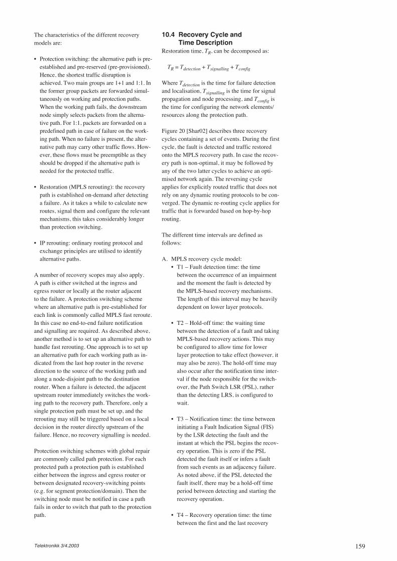
159Telektronikk 3/4.2003
The characteristics of the different recoverymodels are:
• Protection switching: the alternative path is pre-established and pre-reserved (pre-provisioned).Hence, the shortest traffic disruption isachieved. Two main groups are 1+1 and 1:1. Inthe former group packets are forwarded simul-taneously on working and protection paths.When the working path fails, the downstreamnode simply selects packets from the alterna-tive path. For 1:1, packets are forwarded on apredefined path in case of failure on the work-ing path. When no failure is present, the alter-native path may carry other traffic flows. How-ever, these flows must be preemptible as theyshould be dropped if the alternative path isneeded for the protected traffic.
• Restoration (MPLS rerouting): the recoverypath is established on-demand after detectinga failure. As it takes a while to calculate newroutes, signal them and configure the relevantmechanisms, this takes considerably longerthan protection switching.
• IP rerouting: ordinary routing protocol andexchange principles are utilised to identifyalternative paths.
A number of recovery scopes may also apply.A path is either switched at the ingress andegress router or locally at the router adjacentto the failure. A protection switching schemewhere an alternative path is pre-established foreach link is commonly called MPLS fast reroute.In this case no end-to-end failure notificationand signalling are required. As described above,another method is to set up an alternative path tohandle fast rerouting. One approach is to set upan alternative path for each working path as in-dicated from the last hop router in the reversedirection to the source of the working path andalong a node-disjoint path to the destinationrouter. When a failure is detected, the adjacentupstream router immediately switches the work-ing path to the recovery path. Therefore, only asingle protection path must be set up, and thererouting may still be triggered based on a localdecision in the router directly upstream of thefailure. Hence, no recovery signalling is needed.
Protection switching schemes with global repairare commonly called path protection. For eachprotected path a protection path is establishedeither between the ingress and egress router orbetween designated recovery-switching points(e.g. for segment protection/domain). Then theswitching node must be notified in case a pathfails in order to switch that path to the protectionpath.
10.4 Recovery Cycle andTime Description
Restoration time, TR, can be decomposed as:
TR = Tdetection + Tsignalling + Tconfig
Where Tdetection is the time for failure detectionand localisation, Tsignalling is the time for signalpropagation and node processing, and Tconfig isthe time for configuring the network elements/resources along the protection path.
Figure 20 [Shar02] describes three recoverycycles containing a set of events. During the firstcycle, the fault is detected and traffic restoredonto the MPLS recovery path. In case the recov-ery path is non-optimal, it may be followed byany of the two latter cycles to achieve an opti-mised network again. The reversing cycleapplies for explicitly routed traffic that does notrely on any dynamic routing protocols to be con-verged. The dynamic re-routing cycle applies fortraffic that is forwarded based on hop-by-hoprouting.
The different time intervals are defined asfollows:
A. MPLS recovery cycle model:• T1 – Fault detection time: the time
between the occurrence of an impairmentand the moment the fault is detected bythe MPLS-based recovery mechanisms.The length of this interval may be heavilydependent on lower layer protocols.
• T2 – Hold-off time: the waiting timebetween the detection of a fault and takingMPLS-based recovery actions. This maybe configured to allow time for lowerlayer protection to take effect (however, itmay also be zero). The hold-off time mayalso occur after the notification time inter-val if the node responsible for the switch-over, the Path Switch LSR (PSL), ratherthan the detecting LRS, is configured towait.
• T3 – Notification time: the time betweeninitiating a Fault Indication Signal (FIS)by the LSR detecting the fault and theinstant at which the PSL begins the recov-ery operation. This is zero if the PSLdetected the fault itself or infers a faultfrom such events as an adjacency failure.As noted above, if the PSL detected thefault itself, there may be a hold-off timeperiod between detecting and starting therecovery operation.
• T4 – Recovery operation time: the timebetween the first and the last recovery
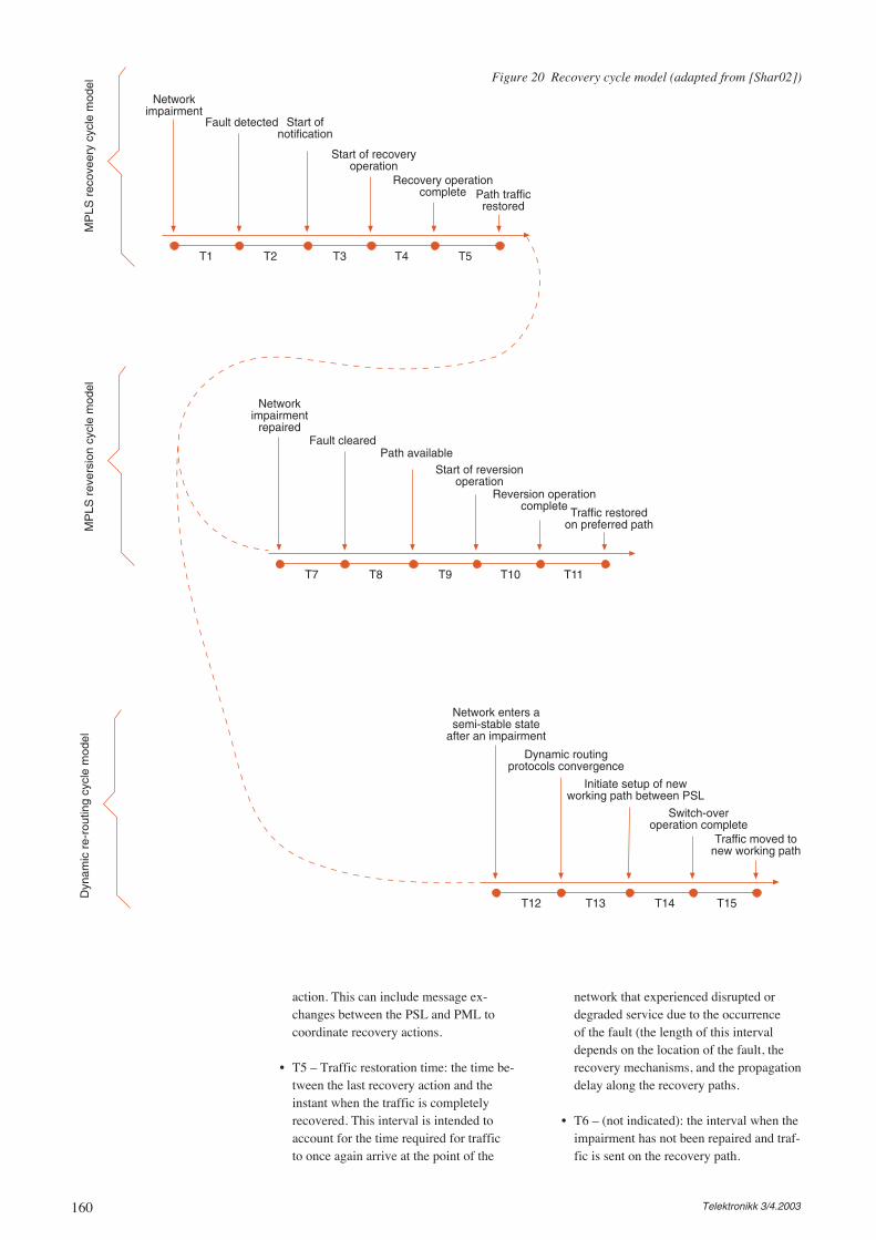
160 Telektronikk 3/4.2003
action. This can include message ex-changes between the PSL and PML tocoordinate recovery actions.
• T5 – Traffic restoration time: the time be-tween the last recovery action and theinstant when the traffic is completelyrecovered. This interval is intended toaccount for the time required for trafficto once again arrive at the point of the
network that experienced disrupted ordegraded service due to the occurrenceof the fault (the length of this intervaldepends on the location of the fault, therecovery mechanisms, and the propagationdelay along the recovery paths.
• T6 – (not indicated): the interval when theimpairment has not been repaired and traf-fic is sent on the recovery path.
Networkimpairment
Fault detected Start ofnotification
Start of recoveryoperation
Recovery operationcomplete Path traffic
restored
T1 T2 T3 T4 T5
Networkimpairment
repairedFault cleared
Path availableStart of reversion
operationReversion operation
complete Traffic restoredon preferred path
T7 T8 T9 T10 T11
Network enters asemi-stable state
after an impairment
Dynamic routingprotocols convergence
Initiate setup of newworking path between PSL
Switch-overoperation complete
Traffic moved tonew working path
T12 T13 T14 T15
MP
LS r
ecov
eery
cyc
le m
odel
MP
LS r
ever
sion
cyc
le m
odel
Dyn
amic
re-
rout
ing
cycl
e m
odel
Figure 20 Recovery cycle model (adapted from [Shar02])

161Telektronikk 3/4.2003
B. MPLS reversion cycle model (executed toswitch the traffic back to the preferred pathafter the fault on that path has been cleared):
• T7 – Fault clearing time: the time betweenthe repair of an impairment and instantwhen the MPLS-based mechanisms learnthat the fault has been cleared. This willlikely be heavily dependent on lower layerprotocols.
• T8 – Wait-to-restore time: the waitingtime between the clearing of a fault andMPLS-based recovery actions. The wait-ing time may be configured to ensure thatthe path is stable and to avoid flapping incases where a fault is intermitted. Thistime may also be set to zero. The waitingtime may occur after the notification timeinterval if the PSL is configured to wait.
• T9 – Notification time: the time betweeninitiating a Fault Recovery Signal (FRS)by the LSR clearing the fault and the timeat which the PSL begins the reversionoperation. This is zero if the PSL clearsthe fault itself. As noted above, there maystill be a Wait-to-restore time period be-tween fault clearing and the start of thereversion operation.
• T10 – Reversion operation time: the timebetween the first and last reversion actions.This may include message exchangesbetween the PSL and PML to coordinatereversion actions.
• T11 – Traffic restoration time: the timebetween the last reversion action andinstant when traffic is completely restoredon the preferred path. This interval isexpected to be small since both paths areworking and care may be taken to limit thetraffic disruption.
In practise, the most interesting times are theWait-to-restore time and the Traffic restora-tion time. As this cycle is completed whenpaths are in operation, there would likely belittle need for a rapid operation. Hence, awell-controlled operation is sought withminimal disruption.
C. Dynamic re-routing cycle model (aims tobring the network to a stable state after im-pairment has occurred. Hence, a re-opti-mised network is sought after the routingprotocols have converged and the traffic hasbeen moved from a recovery path to a (pos-sibly) new working path.
• T12 – Network route convergence time: thetime taken for the routing protocols to con-verge and the network to reach a stable state.
• T13 – Hold-down time: the time for whicha recovery path must be used. This is toprevent flapping of traffic between aworking and a recovery path.
• T14 – Switch-over operation time: thetime between the first and the last switch-over actions. This may include messageexchanges between the PSL and PML tocoordinate the switch-over actions.
• T15 – Traffic restoration time: the timewhen all traffic has been moved to work-ing paths and a new stable network situa-tion reached.
[Huan02] presents a protection mechanismthat is built on the following principles:
• Tree structure for efficient distribution offault and/or recovery information (calledreverse notification tree).
• Hello packets to detect faults as comple-mentary fault detection (in addition to anylower layer mechanism).
• Notification transport protocol, e.g. utilis-ing UDP.
As pointed out in that article, one of the majorconsiderations in a path protection mechanism isto control the delay that must be met by the noti-fication message travelling from the fault detec-tion node to the protection switching node, i.e.POR. This delay may cause additional packetloss and misordering.
A key aspect considered in that article is thatLSPs may be merged; several working pathsmay converge to form a multipoint-to-point treewith the PSLs as leaves. The fault indicationsand repair notifications should then be sentalong a reverse path of the working path to allthe PSLs affected by the fault. This is in case anend-to-end recovery is to be initiated. If a singlesegment is to be recovered, the notificationwould be stopped in the PSL at the beginningof that segment.
Each LSR must be able to detect certain faulttypes, such as path failure, path degraded, linkfailure and link degraded, and send correspond-ing FIS message to the PSL. Hence, a nodeupstream of the fault must be able to detect orlearn about the fault. This motivates for use of ahello protocol commonly using a much shortertimer than applied for most routing protocols.
162 Telektronikk 3/4.2003
11 Concluding RemarksConsidering the steadily increasing growth oftraffic, in particular related to IP-based services,it is essential for an operator to configure an effi-ciently operating network. The interplay of IPand optics has been promoted as a strong candi-date in the core network. This is also the maintopic in this article, with particular emphasis onhow to achieve resilience for the traffic flowsthat have such requirements.
Several studies and international projects havebeen carried out in this area, only a few of theresults and questions are addressed in this arti-cle. Currently it can be observed that several ofthe vendors are taking positions in both the IPand the optics area, also proposing networkingsolutions to manage the topics raised. However,a final answer on how to take care of theresilience seems not to be found yet. Neitheris the general model for IP and optics interplaysettled, advocating for continuing effort.
References[Aute02] Autenrieth, A, Kirstädter, A. Engineer-ing End-to-End IP Resilience Using Resilience-Differentiated QoS. IEEE CommunicationsMagazine, 4 (1), 50–57, 2002.
[Coll02] Colle, D et al. Data-Centric OpticalNetworks and Their Survivability. IEEE Journalon Selected Areas in Communications, 20 (1),6–20, 2002.
[Ho02] Ho, P-H, Mouftah, H T. A Frameworkfor Service-Guaranteed Shared Protection inWDM Mesh Networks. IEEE CommunicationsMagazine, 40 (2), 97–103, 2000.
[Huan02] Huang, C et al. Building ReliableMPLS Networks Using a Path Protection Mech-anism. IEEE Communications Magazine, 40(3),156–162, 2002.
[ID_ipofw] Rajagopalan, B et al. IP over OpticalNetworks: A Framework. IETF draft. Draft-ietf-ipo-framework-05.txt. Oct.2003. Work inprogress.
[ID-iporeq] Xue, Y. Optical Network ServiceRequirements. IETF draft. Draft-ietf-ipo-carrier-requirements-05.txt. Dec 2002. Work inprogress.
[Gers00] Gerstel, O, Ramaswami, R. OpticalLayer Survivability – An Implementation Per-spective. IEE Journal on Selected Areas in Com-munications, 18 (10), 1885–1899, 2000.
[RFC3386] Lai, W, McDysan, D. Network Hier-arch and Multilayer Survivability. IETF RFC3386, Nov. 2002.
[RFC3471] Berger, L. Generalized Multi-Proto-col Label Switching (GMPLS) Signaling Func-tional Description. IETF RFC 3471, Jan. 2003.
[Shar02] Sharma, V, Hellstrand, F. Frameworkfor MPLS-based Recovery. IETF draft Draft-ietf-mpls-recovery-frmwrk-07.txt. Mar. 2002. Workin progress
[Stam00] Stamatelakis, D, Grover, W D. IPLayer Restoration and Network Planning Basedon Virtual Protection Cycles. IEEE Journal onSelected Areas in Communications, 18 (10),1938–1949, 2000.

163Telektronikk 3/4.2003
2.5 GTwo and a half Commonly used term for enhancements in dataGeneration capabilities and bit rates of second generation systems(mobile system) (GSM, TDMA, etc) like EDGE.
2B+DISDN basic ISDN term: 2 channels 64 kbit/s (user traffic), 1 channelaccess 16 kbit/s (signalling, maintenance and user traffic).
30B + DISDN enhanced ISDN term: 30 channels 64 kbit/s (user traffic), 1 channelaccess 64 kbit/s (signalling, maintenance and user traffic).
3G3rd generation The generation of mobile systems which is a (mobile system) descendant of today’s widespread and voice centric
second generation mobile systems like GSM. 3Gsystems are characterised by multimedia capabilityand data rates up to 2 Mbit/s. Ref. UMTS
4G4th generation Term often used to denote future broadband mobile com-(mobile system) munication systems or standards to follow third gene-
ration. Often referred to as “systems beyond 3G” (B3G).
AAAAuthentication, Key functions to intelligently control access, enforceAuthorization policies, audit usage and provide the necessary inform-and Accounting ation for billing of Internet services.
Accounting Tracking which services are used, by whom, when andfor how long. Accounting is carried out by the loggingof session statistics and usage information and is usedfor authorization control billing, trend analysis,resource utilization, and capacity planning activities.
ACTSAdvanced Thematic Programme of the Fourth Framework Communications Research Programme funded by the European Union. It Technologies ran from 1994 to 1998 (the last projects ended in 2000) and Services with a total funding from the EU of 681 million Euro.
http://www.cordis.lu/acts
ADMAdd-dropmultiplexer
Aggregator/ An entity providing access to several underlying net-Aggregation works/systems. This is commonly done by trading ser-broker vices (e.g. bandwidth) between member providers. Bro-
kers typically provide centralized authentication servicesin order to compute and validate the broadband traffic.
APAccess Point A point where users access the system/network,
e.g. a base station in a wireless network.
APSAutomatic Pro-tection Switching
ARIMAAutoregressive Time series modellingIntegrated Moving Average
ASICApplication-Specific Inte-grated Circuit
ASONAutomaticallySwitched OpticalNetwork
ASPApplicationService Provider
ASTNAutomaticallySwitched Trans-port Network
ATMAsynchronousTransfer Mode
AUCAuthenticationCentre
Authentication The process of determining who the user is. It can takethe form of ensuring that data has come from itsclaimed source, or of corroborating the claimed identityof a communication party.
Authentication The server that is responsible for authenticating theserver content user {source [BCD01a]}.
Authorization The process of enforcing policies – of determining thetypes or qualities of activities, resource, or services auser is permitted. Usually, authorization is in the con-text of authentication; once you have authenticated auser, (s)he may be authorized for different types ofaccess or activities.
Authorization Determines if an authenticated user is authorized toserver view content with a particular set of delivery para-
meters. May also bill the user for use and generate abilling record that is sent to the content provider. Thecontent provider or a third-party could own this server{source [BCD01a]}.
B-ISDNBroadbandIntegratedServices DigitalNetwork
BABehaviour A collection of packets with the same (DiffServ) codeAggregate point crossing a link in a particular direction.
{source [RFC3564]}
Baseline A study conducted to serve as a baseline for com-analysis paring to the actual behaviour of the network.
{source [RFC3272]}
Billing cycle The period between the creation of billing files. Typi-cally, this is done once a day at a specific time. Thebilling file contains the traffic of all end users per roam-ing partner for one billing cycle. The shorter the billingcycle, the better the risk of fraud can be monitored inroaming environments.
BLSRBi-directionalline switchedring
Terms and Acronyms
Note: Several of the acronyms have been described in articles of this issue.
164 Telektronikk 3/4.2003
Bluetooth A short-range wireless specification that allows radioconnection between devices within a 10-metre rangeof each other. Bluetooth is designed as a Personal AreaNetwork (PAN) technology with a wide variety oftheoretical uses.
BGPBorder GatewayProtocol
BOTBuild, operate Telenor product offering to cover deployment,and Telenor operation and maintenance of ICT equipment incollocation addition to collocation of technical equipment.
Bottleneck A network element whose input traffic rate tends to begreater than its output rate. {source [RFC3272]}
Branch and A tree of linear programs is formed in which eachbound problem has the same constraints and objectives except
for some additional bounds on certain variables. At theroot of this tree is the original problem without addi-tional requirements. The solution to this root problemwill not, in general, have all integer components. Wenow choose some non-integer solution component anddefine two variants by fixing one of the variables. Thisgives rise to two sub-problems. The left-child andright-child problems separate the solution space. Thisbranching process can be carried out recursively; eachof the two new problems will give rise to two moreproblems when we branch on one of the non-integercomponents of their solution. It follows from thisconstruction that the tree is binary.Eventually, after enough new bounds are placed on thevariables, integer solutions are obtained. The value forthe best integer solution found so far is retained andused as a basis for pruning the tree. If the continuousproblem at one of the tree nodes has a final objectivevalue different from the value obtained in a node, sohave all of the node’s descendants, since they havesmaller feasible regions and hence even larger optimalobjective values. The branch emanating from such anode cannot give rise to a better integer solution thanthe one obtained so far, so we consider it no further;that is, we prune it. Pruning also occurs when we haveadded so many new bounds to some continuous prob-lem that its feasible region disappears altogether.Two strategies for solving the node problems aredepth-first and width-first, of which the former isfrequently preferred.
BRASBroadbandRemote AccessServer
BSCBase Station Network node in the GSM network controlling aController number of BTSs. http://www.etsi.org
BTSBase Trans- The radio base station of a GSM network. It consists ofceiver Station one or more transmitter-receiver units, each serving
one carrier frequency. http://www.etsi.org
Busy hour A one hour period within a specified interval of time(typically 24 hours) in which the traffic load in a net-work or sub-network is greatest. {source [RFC3272]}
BWBandwidth
Bypass tunnel A path that serves to back up a set of working pathsusing the label stacking approach. The working pathsand the bypass tunnel must all share the same PSL andPML {source [Shar02]}.
CAPEXCapital Expenses
CAPMCapital AssetPricing Model
CaTVCable TV
CDMACode Division Multiple access method used e.g. in UMTS. AllowingMultiple Access for multiple transmissions to be carried simultaneously
on a single wireless channel (same time slot and carrierfrequency). This is done by spreading the signal acrossthe frequency band using one of a set of spreadingcodes such that one user’s signal appears as noise/interference for other (non-intentional) receivers.
CDNContent A collection of network elements arranged for moreDistribution/ effective delivery of content to clients. Typically aDelivery CDN consists of a request-routing system, surrogatesNetwork (a content server other than the origin server), a distri-
bution network, and an accounting system. {source[BCD01a] – from IETF content peering group}
Clearing house A provider of roaming billing data services. A clearinghouse typically provides post-connection services byhandling the billing data, offering validation and ratingservices as well as settling the financial liabilities. Adistinction should be made between data and financialclearing house. The latter is also referred to as settle-ment house. The former only delivers the data process-ing service whereas the latter also provides invoice andpayment services.
Congestion A state of a network resource in which the traffic inci-dent on the resource exceeds its output capacity over atime interval. {source [RFC3272]}
Congestion An approach to congestion management that attemptsavoidance to obviate the occurrence of congestion.
{source [RFC3272]}
Congestion An approach to congestion management that attemptscontrol to remedy congestion problems that have already
occurred. {source [RFC3272]}
Constraint A class of routing protocols that take specified trafficbased attributes, network constraints, and policy constraints routing into account when making routing decisions. Constraint-
based routing is applicable to traffic aggregates as wellas flows. It is a generalization of QoS routing. {source[RFC3272]}
Content A conceptual identifier of a media object and its con-stituent digital bit streams. An identifier is a movietitle, a song name, and – in the case of a live event – anevent identifier. Note that content could be comprisedof several different bit streams. For example, a particu-lar movie could be encoded in three different qualitiesand have several language tracks. A live event could alsobe encoded in different qualities. {source: [BCD01a]}
Content server The server that is responsible for sending the stream toa target device over some network. This may be theoriginal server or a surrogate server owned by the con-tent network.
CPUCentral Pro-cessing Unit
CTClass Type The set of Traffic Trunks crossing a link that is
governed by a specific set of bandwidth constraints.CT is used for the purposes of the link bandwidth allo-cation, constraint based routing and admission control.A given Traffic Trunk belongs to the same CT on alllinks. {source [RFC3564]}
165Telektronikk 3/4.2003
CWDMCoarse wave- A relatively low-cost WDM technology that uses widelength division spacing (about 10 nm) between wavelengths andmultiplexing un-cooled optics.
DACSDigital accesscross-connectsystem
DBDatabase
DCFDiscountedCash Flow
DCMEDigital CircuitMultiplicationEquipment
Demand side A congestion management scheme that addressescongestion congestion problems by regulating or conditioningmanagement offered load. {source [RFC3272]}
Dijkstra’s An algorithm to find the shortest paths from a singlealgorithm source node to all other nodes in a weighted, directed graph.
DPPDiscountedPayback Period
DPRingsDedicated pro-tection rings
DRMDigital RightsManagement
DSDiffServ– DifferentiatedServices
DSLDigital Sub-scriber Line
DSLAMDigital sub-scriber lineaccess module
DSMDynamicspectrummanagement
DTHDirect to home Satellite access
DWDMDense A carrier-class WDM technology that uses expensive,wavelength cooled optics and tight spacing between wavelengths division of less than a nanometre based on the specifications of multiplexing the International Telecommunications Union (ITU)
DWDM wavelength grid. http//www.itu.int
E-LAN service Ethernet LAN service provides multipoint connectivityby connecting two or more users. One or more of theconnected users can receive data. At each site the useris connected to a multipoint Ethernet Virtual Connec-tion (EVC). As new sites are added they are connectedto the same multipoint EVC. From a user point of viewthe E-LAN service makes the carrier network (metroand wide areas) look like a switched LAN. For an easycomparison the Virtual Private Line Service (VPLS)
can be seen as an E-LAN service that is centred on theuse of MPLS labels in the forwarding plane as opposedto the use of CLAN tags in the Metro Ethernet Forum(MEF) definitions. Both E-LAN and VPLS focus onenabling carriers to deliver true VPN services to users.{source [MEFsite]}
E-Line service Ethernet line service providing point-to-point EthernetVirtual Connection (EVC) between two subscribers.The E-line service is used for Ethernet point-to-pointconnectivity. {source [MEFsite]}
EBITEarnings BeforeInterests andIncome Taxes
EBITDAEarnings BeforeIncome Taxes,Depreciation andAmortisation
EDGEEnhanced Data A modulation method for GSM and IS-136 TDMAfor GSM networks that allows for wireless data transfer up toEvolution 384 kbit/s. Standardized by ETSI. http://www.etsi.org
Edge server A network element close to the edge of a backbone net-work that is able to perform content services. Serviceexamples include caching, video/audio stream servingand splitting, insertion, transcoding, content listing, etc.{source [BCD01a]}
Effective The minimum amount of bandwidth that can bebandwidth assigned to a flow or traffic aggregate in order to
deliver ‘acceptable service quality’ to the flow ortraffic aggregate.
Egress traffic Traffic exiting a network or network element.
EIREquipmentIdentity Register
EPGElectronic Pro-gramme Guide
Erlang’s Well-applied formula for calculating the blockingblocking probability (used for decades in telephony networks).formula
Ethernet International standard networking technology forwired implementations. Basic, traditional networksoffer a bandwidth of about 10 Mbit/s. Fast Ethernet(100 Mbit/s) and Gigabit Ethernet (1000 Mbit/s), aswell as 10 Gigabit, are also available.
ETSIEuropean Tele- A non-profit membership organisation founded incommunications 1988. The aim is to produce telecommunicationsStandards standards to be used throughout Europe. The efforts areInstitute coordinated with the ITU. Membership is open to any
European organisation proving an interest in promotingEuropean standards. It was responsible for the makingof the GSM standard, among others. The headquartersare in Sophia Antipolis, France. http://www.etsi.org
Extra traffic Traffic carried over the protection entity while the(also referred to working entity is active. Extra traffic is not protected,as pre-emptable i.e. when the protection entity is required to protect thetraffic) traffic that is being carried over the working entity, the
extra traffic is pre-empted. {source [RFC3386]}
FECForward Equi-valence Class
166 Telektronikk 3/4.2003
FISFault Indication A signal that indicates that a fault along a path hasSignal occurred. It is relayed by each intermediate LSR to its
upstream or downstream neighbour until it reaches anLSR that is set up to perform MPLS recovery (thePOR). The FIS is transmitted periodically by the node(closest to the point of failure) for some configurablelength of time. {source [Shar02]}
Forecasting Statement in advance of traffic characteristics, includ-traffic ing volume (e.g. measured in Mbit/s) and number of
customers.
Flow The term flow is commonly used to signify the smallestnon-separable stream of data from the point of view ofan end-point or termination point (source or destinationpoints). {based on [ID-ipofw]}
Footprint A network of access points referring to the overallcoverage of the network.
FRSFault Recovery A signal that indicates that a fault along a working path Signal has been repaired. Again, like the FIS, it is relayed by
each intermediate LSR to its upstream or downstreamneighbour until it reaches the LSR that performs recov-ery of the original path. The FRS is transmitted periodi-cally by the node/nodes closest to the point of failurefor some configurable length of time. {source [Shar02]}
FTPFile TransferProtocol
FTTHFibre to the home
FWAFixed Wireless Fixed Wireless Access consists of a radio link to theAccess home or the office from a cell site or base station. It
replaces the traditional wireless local loop, either if thewire based infrastructure is sparse or to gain rapidexpansion in denser urban and suburban areas.
GBGigabit ‘One billion bits’. Term used to denote the number
1 073 741 824 bits (230).
GMPLSGeneralizedMulti-ProtocolLabel Switching
GoSGrade of Service
GPRSGeneral Packet An enhancement to the GSM mobile communicationsRadio Service system that supports data packets. GPRS enables con-
tinuous flows of IP data packets over the system forsuch applications as web browsing and file transfer.Supports up to 160 kbit/s gross transfer rate. Practicalrates are from 12–48 kbit/s. http://www.etsi.org
Greenfield A service provider that introduces itself to a newprovider market/region without prior engagements.
GSMGlobal System A digital cellular phone technology that is the pre-for Mobile dominant system in Europe, but is also used aroundcommunication the world. Development started in 1982 by CEPT and
was transferred to the new organisation ETSI in 1989.Originally, the acronym was the group in charge,‘Groupe Special Mobile’, but later the group changedits name to SMG, and GSM became the name of thesystem. GSM was first deployed in seven Europeancountries in 1992. It operates in the 900 MHz and1.8 GHz bands in Europe and the 1.9 GHz PCS band
in North America. GSM defines the entire cellular sys-tem, from the air interface to the network nodes andprotocols. As of 2000 there were more than 250 millionGSM users, which is more than half the world’s mobilephone population. http://www.etsi.org
GSM Alliance Consortium of North American GSM 1900 operators.
GSM World’s leading wireless industry representative body, Association consisting of more than 660 second- and third-genera-
tion wireless network operators and key manufacturersand suppliers to the wireless industry.www.gsmworld.com
HB@Hybrid Broad- Telenor project running from 2000–2002 with the aim band Access of investigating and testing how different access tech-
nologies could be combined in order to develop a com-plete broadband network able to provide comparablebroadband services both in urban, suburban and ruralparts. The aim was to develop Telenor’s superior strat-egy and specific solutions on the implementation androll-out of a hybrid access infrastructure suitable fortelevision and personal computer centric broadbandservices in the period 2001–2005.Four different technical solutions were tested inStavanger, Svolvær, Beito and Oslo providing a selec-tion of next generation interactive broadband services.http://www.telenor.no/prosjekt/hba/indeks.shtml (inNorwegian)
HDTVHigh DefinitionTV
HFCHybrid FibreCoax
Hierarchy A technique used to build scalable complex systems.It is based on an abstraction, at each level, of what ismost significant regarding the details and internalstructures of the levels further away. This approachmakes use of a general property of all hierarchical sys-tems composed of relevant subsystems that interactionsbetween subsystems decrease as the level of communi-cation between subsystems decreases.
HLRHome Location A database that holds subscription information aboutRegister every subscriber in a mobile network. An HLR is a per-
manent SS7 database used in cellular networks. TheHLR is located at the SCP (Signal Control Point) of thecellular provider of record, and is used to identify/ver-ify a subscriber. It also contains subscriber data relatedto features and services. http://www.etsi.org
Home operator The provider that owns the relationship with the userof the service by way of a subscription agreementallowing the provider to bill the user for services.
Horizontal The abstraction that allows a network at one tech-hierarchy nology layer, for instance a packet network, to scale.
Examples of horizontal hierarchy include BGP confed-erations, separate autonomous systems and multi-areaOSPF. In the horizontal hierarchy, a large network ispartitioned into multiple smaller, non-overlapping sub-networks. The partitioning criteria can be based ontopology, network function, administrative policy, orservice domain demarcation. Two networks at the“same” hierarchical level, e.g. two autonomous sys-tems in BGP, may share a peer relation with each otherthrough some loose form of coupling. On the otherhand, for routing in large networks using multi-areaOSPF, abstraction through the aggregation of routinginformation is achieved through a hierarchical parti-tioning of the network. {source [RFC3386]}
167Telektronikk 3/4.2003
Hot spot • A venue where a commercial public WLAN servicecan be accessed. Hotspots are typically found inhotels, airports and cafés.
• A network element or subsystem, which is in a stateof congestion. {source [RFC3272]}
HSCSDHigh speed An addition to GSM for adding faster data trans-circuit switched mission. While GSM originally supports 9.6 kbit/s,data HSCSD supports from 14.4 up to 57.6 kbit/s circuit
switched data connections. http://www.etsi.org
HSSGHigher speed The group commissioned by the IEEE 802.3 Ethernetstudy group working group with drafting the technical scope and
objectives of the standards effort.
Hub A multi-port device used to connect PCs to a network,typically via Ethernet cabling or via wireless access(WLAN). Wired hubs can have numerous ports andcan transmit data at speeds ranging from 10 Mbit/s tomulti-gigabyte rates per second. A hub transmits thepackets it receives to all the connected ports. A smallwired hub may only connect four computers; a largehub can connect 48 or more, whereas a wireless hubcan connect hundreds.
ICTInformation andcommunicationtechnologies
IECInternational An organization that sets international electrical andElectrotechnical electronics standards founded in 1906. It is made up ofCommission national committees from over 40 countries. Headquar-
ters in Geneva, Switzerland. http://www.iec.ch
IEC/ISO 11801 The international and European standard for buildingcabling.
IEEEThe Institute USA based organisation open to engineers andof Electrical researchers in the fields of electricity, electronics,and Electronics computer science and telecommunications. EstablishedEngineers in 1884. The aim is to promote research through jour-
nals and conferences and to produce standards intelecommunications and computer science. IEEE hasproduced more than 900 active standards and has morethan 700 standards under development. Divided intodifferent branches, or ‘Societies’. Has daughter organi-sations, or ‘chapters’ in more than 175 countries world-wide. Headquarters in Piscataway, New Jersey, USA.http://www.ieee.org
IEEE 802.11 Refers to a family of specifications developed by theIEEE for wireless local area networks. It also refers tothe “Wireless LAN working group” of the IEEE 802project. 802.11 specifies an over-the-air interfacebetween a wireless client and a base station, or betweentwo wireless clients. The IEEE accepted the specifica-tion in 1997. There are several specifications in the802.11 family, including i) 802.11 – provides 1 or 2Mbit/s transmission in the 2.4 GHz band; ii) 802.11a –an extension that provides up to 54 Mbit/s in the 5 GHzband (it uses an orthogonal frequency division multi-plexing encoding scheme rather than FHSS or DSSS);iii) 802.11b – provides 11 Mbit/s transmission in the2.4 GHz band and was ratified in 1999 allowing wire-less functionality comparable to Ethernet; iv) 802.11gprovides 20+ Mbit/s in the 2.4 GHz band; v) 802.11zis a method for transporting an authentication protocolbetween the client and access point, and the TransportLayer Security (TLS) protocol. More variants are alsounder preparation, including support of 100 Mbit/straffic flows. http://www.ieee802.org/11/
IEEE 802.3 The permanent CSMA/CD (Ethernet) working groupWorking Group of the IEEE 802 project. http://www.ieee802.org/3/
IEEE 802.3ae The Task Force chartered by the IEEE 802.3 workingTask Force group with writing the specification for 10 Gigabit
Ethernet. IEEE 802.3ae is also the name of the docu-ment produced by the Task Force.http://www.ieee802.org/3/ae/index.html
IETFThe Internet The Internet Engineering Task Force is a large openEngineering international community of network designers,Task Force operators, vendors, and researchers concerned with the
evolution of the Internet architecture and the smoothoperation of the Internet. It is open to any interestedindividual. The actual technical work of the IETF isdone in its working groups, which are organized bytopic into several areas (e.g. routing, transport, security,etc.). The IETF working groups are grouped into areas,and managed by Area Directors (AD). The ADs aremembers of the Internet Engineering Steering Group(IESG). Providing architectural oversight is the InternetArchitecture Board, (IAB). The IAB also adjudicatesappeals when someone complains that the IESG hasfailed. The IAB and IESG are chartered by the InternetSociety (ISOC) for these purposes. The General AreaDirector also serves as the chair of the IESG and of theIETF, and is an ex-officio member of the IAB.http://www.ietf.org
IGPInternal Gate-way Protocol
IMInstant Message
INIntelligentNetwork
Industry A non-profit organisation that helps to create commonorganisation technical or commercial recommendations and specifi-
cations that streamline the marketplace.
Ingress traffic Traffic entering a network or network element. {source [RFC3272]}
Integer Optimisation formulation with integer constraints onprogramming some variables.
Integrator A company that offers consulting services to help puteverything together.
Inter-domain Traffic that originates in one autonomous system andtraffic terminates in another. {source [RFC3272]}
Intermediate An LSR on a working or recovery path that is neither aLSR PSL nor a PML for that path. {source [Shar02]}
IPInternet Protocol A protocol for communication between computers,
used as a standard for transmitting data over networksand as the basis for standard Internet protocols.http://www.ietf.org
IOTInter Operator Rate that the settlement price between Wireless ISPsTariff for roaming traffic is based on. The roaming agreement
between the home and the visited WISPs regulates therebate (if any) that the home operator is entitled to relativeto the IOT. The IOT is often roughly equal to the normalper minute price for users in the operator’s network.
IRRInternal rate ofreturn
168 Telektronikk 3/4.2003
ISDNIntegrated A digital telecommunication network that providesServices Digital end-to-end digital connectivity to support a wide rangeNetwork of services, including voice and non-voice services, to
which users have access by a limited set of standardmulti-purpose user-network interfaces. The user isoffered one or more 64 kbit/s channels. http://www.itu.int
ISOInternational The International Organization for StandardizationOrganization for (ISO) is a world-wide federation of national standardsStandardization bodies from more than 140 countries, one from each
country. ISO is a non-governmental organization estab-lished in 1947. The mission of ISO is to promote thedevelopment of standardization and related activities inthe world with a view to facilitating the internationalexchange of goods and services, and to developingcooperation in the spheres of intellectual, scientific,technological and economic activity. http://www.iso.org/
ISPInternet Service A vendor who provides access for customers to theProvider Internet and the World Wide Web. The ISP also
typically provides a core group of Internet utilitiesand services like e-mail and news group readers.
ISTInformation Thematic Programmes of the 5th and 6th FrameworkSociety Research Programmes funded by the European Union.Technologies The first IST programme runs from 2000 to 2004, while
the IST programme of the 6th Framework ResearchProgramme started in 2003 and will run until 2006.http://www.cordis.lu/ist/
ITUInternational The ITU is a United Nations (UN) body with approx.Telecommuni- 200 member countries. It is the top forum for dis-cation Union cussion and management of technical and administra-
tive aspects of international telecommunications. Itsmain objective is to promote connectivity and inter-operability between its member countries and to fosterthe development of all kinds of telecommunicationsworldwide. It was established in 1865 as an intergov-ernmental organization with the aim of streamlininginterconnection of the national telegraph networks.In 1947 it became a specialized agency of the UN.http://www.itu.int
ITVInteractive TV
LDLink Degraded A lower layer indication to MPLS-based recovery
mechanisms that the link is performing below anacceptable level. {source [Shar02]}
LEXLocal Exchange
LFLink Failure A lower layer fault indicating that link continuity is lost.
This may be communicated to the MPLS-based recov-ery mechanisms by the lower layer. {source [Shar02]}
LIBLabel Inform-ation Base
Link-disjoint Two connections are link-disjoint if they do not shareany link along the path.
Liveness A message exchanged periodically between twomessage adjacent LSRs that serves as a link proving mechanism.
It provides an integrity check of the forward and back-ward directions of the link between the two LSRs as wellas a check of neighbour aliveness. {source [Shar02]}
LLLeased Line
LLUBLocal Loop Option to rent only the local loop (e.g. copper accessUnbundling line to a customer) by a non-incumbent operator.
LMDSLocal Multipoint System for Wireless Local Loop applications whichDistribution can replace cable based access to private and corporateSystem customers. Typically operates in the millimetre wave
band. Can provide bandwidth of several Mbit/s to theend customer.
Loss network A network that does not provide adequate buffering fortraffic, so that traffic entering a busy resource withinthe network will be dropped rather than queued.{source [RFC3272]}
LPLocation Point
LSLocal switch
LSPLabel SwitchedPath
LSRLabel SwitchingRouter
MACMedia accesscontrol protocol
MAC AddressMedia Access A hardwire address that uniquely identifies each nodeControl of a network.
Management The process by which managers assure that resourcescontrol/tactical are obtained and used effectively and efficiently in theplanning accomplishment of the organisation’s objective.
{source [Anth65]}
Mbit/sMegabit per ‘One million bits per second’. Term used to denote asecond data signalling rate of 1 048 576 b/s (220).
MDMain distribu-tion point
Measurement Measurements can be classified on the basis of wherebasis and at which level of aggregation the traffic data are
gathered. This refers to a set of packets, possibly rela-tive to a particular pair of source and destination, forthe purposes of defining performance parameters.Typical measurement bases are; flow-based, interface-based, link-based, node-based, node-pair-based, path-based. {source [ID_Temea03]}
Measurement A measurement entity defines what is measured; it is aentity quantity for which data collection must be performed
with a certain measurement. A measurement type canbe specified by a (meaningful) combination of a mea-surement entity with the measurement basis. {source[ID_Temea03]}
Measurement A measurement interval is the time interval over whichinterval measurements are taken. Some traffic data are collected
continuously, while other data are collected by sam-pling, or on a scheduled basis. A measurement intervalconsists of a sequence of consecutive read-out periods.Summarisation is usually done by integrating the rawdata over a pre-specified read-out period. The periodmust be short enough to capture – with acceptableaccuracy – the bursty nature of the traffic, while notbeing so short that the volume of data produced getstoo voluminous.
MPLS label The hop between two MPLS nodes, on which forward-switch hop ing is done by use of labels. {from [RFC3031]}
MPLS label The path through one of more Label Switched Routersswitched path (LSRs) at one level of the hierarchy followed by a
packet of a particular FEC. {from [RFC3031]}
MPLS merge A node at which label merging is done. {frompoint [RFC3031]}
MPLS node A node which runs MPLS. An MPLS node will beaware of MPLS control protocols, will operate one ormore layer 3 routing protocols, and will be capable offorwarding packets based on labels. {from [RFC3031]}
MPLS The set of LSRs over which a working path and itsprotection corresponding recovery path are routed. {source domain [Shar02]}
MPLSprotection plan The set of all LSP protection paths and the mapping
from working to protection paths deployed in an MPLSprotection domain at a given time. {source [Shar02]}
MRAMultilateral Cooperation agreement between a wireless ISP and aRoaming central legal entity where the former guarantees theAgreement provision of services to the need users of the members
of the latter. The central legal entity guarantees thesetting of minimum standards of service for existingand future members. The result of the cooperationagreement is that end users can roam in the networkof the members of the platform.
MSCMobile Switch- The switching node in a GSM network.ing Centre http://www.etsi.org
MTXMobile The switching node in an NMT network.TelephoneExchange
MVNOMobile Virtual An actor offering mobile services not having its ownNetwork mobile network, but relying on other actors to provideOperator the network resources. (Ref. Telektronikk, 97 (4), 2001)
NBNarrowband
NCFNet Cash Flow
NENetworkElement
Network Handover of an uninterrupted session between differenthandover networks or access points.
Network An abstraction of part of a network’s topology, routinghierarchy and signalling mechanism. The abstraction may be
used as a mechanism to build large networks or as atechnique to enforce administrative, topological, orgeographic boundaries. For example, network hierar-chy might be used to separate the metropolitan andlong-haul regions of a network, or to separate theregional and backbone sections of a network, or tointerconnect service provider networks (with BGPwhich reduces a network to an autonomous system).Two perspectives may be taken on:• Vertically oriented: between two network technology
layers;• Horizontally oriented: between two areas or adminis-
trative subdivisions within the same network tech-nology layer. {source [RFC3386]}
169Telektronikk 3/4.2003
Measurement A repeatable measurement technique used to derivemethodology one or more metrics of interest. {source [RFC3272]}
Metric A parameter defined in terms of standard units ofmeasurement. {source [RFC3272]}
Mesh optical A topologically connected collection of optical sub-network networks whose node degree may exceed 2. Such an
optical network is assumed to be under purview of asingle administrative entity. It is also possible to con-ceive a large scale global mesh optical network consist-ing of the voluntary interconnection of autonomousoptical networks, each of which is owned and adminis-tered by an independent entity. In such an environment,abstraction can be used to hide the internal details ofeach autonomous optical cloud from external clouds.{based on [ID-ipofw]}
MONMetropolitanOptical Network
MPEGMoving Pictures MPEG is a committee of ISO/IEC that is open toExpert Group experts duly accredited by an appropriate National
Standards Body. It is in charge of the development ofstandards for coded representation of digital audio andvideo. Established in 1988, the group has producedMPEG-1, the standard on which such products asVideo CD and MP3 are based, MPEG-2, the standardon which such products as Digital Television set topboxes and DVD are based, MPEG-4, the standard formultimedia for the fixed and mobile web and MPEG-7,the standard for description and search of audio andvisual content. Work on the new standard MPEG-21“Multimedia Framework” has started in June 2000.http://www.chiariglione.org/mpeg/
MPLSMulti Protocol An IETF standard intended for Internet application.Label Switching A widely supported method of speeding up IP-based
data communication. {RFC 2702}
MPLS domain A continuous set of nodes which operate MPLS routingand forwarding and which are also in one routing ofadministrative domain. {from [RFC3031]}
MPLS edge An MPLS node that connects an MPLS domain with a node node which is outside of the domain, either because it
does not run MPLS and/or because it is in a differentdomain. Note that if an LSR has a neighbouring hostwhich is not running MPLS, that LSR is an MPLS edgenode. {from [RFC3031]}
MPLS egress An MPLS edge node in its role in handling traffic as itnode leaves an MPLS domain. {from [RFC3031]}
MPLS ingress An MPLS edge node in its role in handling traffic as itnode enters an MPLS domain. {from [RFC3031]}
MPLS label A label which is carried in a packet header and whichrepresents the packet’s FEC. A short fixed length phys-ically continuous identifier used to identify an FEC oflocal significance. {from [RFC3031]}
MPLS label The replacement of multiple incoming labels for a partic-merging ular FEC with a single outgoing label. {from [RFC3031]}
MPLS label An ordered set of labels. {from [RFC3031]}stack
MPLS label The basic forwarding operation consisting of lookingswap up an incoming label to determine the outgoing label,
encapsulating, port, and other data handling informa-tion. {from [RFC3031]}
MPLS label A forwarding paradigm allowing streamlined forward-swapping ing of data by using labels to identify classes of data
packets which are treated indistinguishably whenforwarding. {from [RFC3031]}
170 Telektronikk 3/4.2003
Network The capability to provide a prescribed level of QoS forsurvivability existing services after a given number of failures occur
within the network. {source [RFC3272]}
Next-gen SDH Including the Ethernet functionality in SDH andSONET equipment using GFP, LCAS and virtualconcatenation. Next-gen SDH may also supportvirtual switching, including multipoint connections.
NHLFENext Hop LabelForwarding Entry
NMTNordic mobile Automatic mobile telephone system based on analoguetelephony transmission technology. NMT was developed by the
Nordic public telephone administrations (Norway,Sweden, Denmark, Finland and Iceland) in the period1969 to 1980. The first version operated in the 450 MHzband (NMT-450) and was launched in 1981/1982.Later the system was enhanced to operate in the900 MHz band (NMT-900, 1986). The system offeredvoice telephony with international roaming. The tech-nology used was narrowband frequency modulation(FM) with 25 kHz user channels. The NMT-900 ser-vice was discontinued to release the frequencyresources in 2001 when the GSM coverage had reacheda sufficiently high level. In Norway the NMT-450 sys-tem will be discontinued at the end of 2004. (Ref.Telektronikk, 91 (4), 1995)
NNINetwork-Network Interface
Node-disjoint Two connections are node-disjoint if they do not shareany node along the path except the ingress and egressnodes.
Non-revertive Case where there is no preferred path or it may bemode desirable to minimize further disruption of the service
brought on by a revertive switching operation. Aswitch-back to the original working path is not desiredor not possible since the original path may no longerexist after the occurrence of a fault on that path. {source[RFC3386]}A recovery mode in which traffic is not automaticallyswitched back to the original working path after thispath is restored to a fault-free condition. {source[Shar02]}
NOCNetwork The physical space from which a typically largeOperations telecommunication network is managed, monitored andCentre supervised. The NOC coordinates network troubles,
provides problem management and router configura-tion services, manages network changes, allocates andmanages domain names and IP addresses, monitorsrouters, switches, hubs and UPS that keep the networkoperating smoothly, manages the distribution andupdating of software and coordinates with affiliatednetworks.
Normalization Sequence of events and actions taken by a network thatreturns the network to the preferred state upon complet-ing repair of a failure. This could include the switchingor rerouting of affected traffic to the original repairedworking entities or new routes. Revertive mode refersto the case where traffic is automatically returned to arepaired working entity (also called switch-back).{source [RFC3386]}
NPNetworkPerformance
NPVNet presentvalue
NSPNetwork ServiceProvider
NVoDNear Videoon Demand
OAOrdered A set of BAs that share an ordering constraint. The setAggregate of PHBs that are applied to this set of Behaviour
Aggregates constitutes a PHB scheduling class. {source [RFC3564]}
OA&MOperation,Administration & Maintenance
OBLSROptical bi-directional lineswitched ring
OBPSROptical bi-directional pathswitched ring
OChOptical Channel
Offline traffic A traffic engineering system that exists outside of theengineering network. {source [RFC3272]}
OIFOptical Inter-working Forum
OMSOptical The optical multiples section layer provides transportMultiplex for the optical channels. The information contained inSection – this layer is a data stream comprising a set of opticallayer network channels, which may have a defined aggregate band-
width.
Online traffic A traffic engineering system that exists within theengineering network, typically implemented on or as adjuncts to
operational network elements. {source [RFC3272]}
Opaque vs. A transparent optical network is an optical network intransparent which optical signals are transported from transmitteroptical networks to receiver entirely in the optical domain without OEO
conversion. Generally, intermediate switching nodes ina transparent optical network do not have access to thepayload carried by the optical signals. Note that ampli-fication of signals at transit nodes is permitted in trans-parent optical networks.On the other hand, in opaque optical networks transitnodes may manipulate optical signals traversingthrough them. An example of such manipulation wouldbe OEO conversion which may involve 3R operations(reshaping, retiming, regeneration, and perhaps ampli-fication). {based on [ID-ipofw]}
Operational The process of assuring that specific tasks are carriedcontrol out effectively and efficiently. {source [Anth65]}
OPEXOperationsExpenses
OPPROptical pathprotection ring
171Telektronikk 3/4.2003
Optical channel An optical channel trail is a point-to-point optical layertrail of lightpath connection between two access points in an optical
network. {based on [ID-ipofw]}
Optical An optical internetwork is a mesh-connected collectioninternetwork of optical networks. Each of these networks may be
under a different administration. {based on [ID-ipofw]}
Optical mesh An optical sub-network is a network of OXCs thatsub-network supports end-to-end networking of optical channel
trails providing functionality like routing, monitoring,grooming, and protection and restoration of opticalchannels. The interconnection of OXCs in this networkcan be based on a general mesh topology. The follow-ing sub-layers may be associated with this network.
OPTIMUMOptimised Research project in the European Union’s 4th Frame-Network Archi- work Research Programme ACTS. The objective of thetectures for project was to establish guidelines for the introductionMultimedia of advanced communications networks and multimediaServices services in a competitive multiservice environment.
The project used techno-economic evaluation of differ-ent case studies derived from field trials and projectswithin and outside ACTS. Project duration was from1996 to 1998. http://www.cordis.lu/infowin/acts/rus/projects/ac226.htm,http://www.telenor.no/fou/prosjekter/optimum/
OSIOpen System Reference model from ISO for data communicationInterconnection divided into 7 main layers; 1 – physical, 2 – data link,
3 – network, 4 – transport, 5 – session, 6 – presenta-tion, 7 – application.
OSPFOpen ShortestPath First
OSPROptical sharedprotection ring
OSSOperationsSupport System
OTNOptical Trans-port Network
OTNTOptical Trans-port Networks &Technologies
OTSOptical Trans- This layer provides functionality for transmission ofmission Section optical signals through different types of optical media.– layer network {based on [ID-ipofw]}
OULSROptical unidi-rectional line-switching ring
OUPSROptical unidi-rectional path-switched ring
OXCOptical A space-division switch that can switch an optical dataCross-Connect stream from an input port to an output port. Such a
switch may utilise optical-electrical conversion at theinput port and electrical-optical conversion at the out-put port, or it may be all-optical. An OXC is assumedto have a control plane processor that implements the
signalling and routing protocols necessary for comput-ing and instantiating optical channel connectivity in theoptical domain. {based on [ID-ipofw]}
P2PPeer-to-Peer
Path continuity A test that verifies the integrity and continuity of a pathtest or path segment. {source [Shar02]}
PDHPlesiochronousDigital Hierarchy
Peering A collection of network elements supporting someform of interconnected operation among two or moreentities owned by separate organizations. Examplesinclude accounting peering, content list peering anddistribution peering. {source [BCD01a]}
Performance A systematic approach to improving effectiveness inmanagement the accomplishment of specific networking goals
related to performance improvement. {source[RFC3272]}
Performance Metrics that provide quantitative or qualitativemeasures measures of the performance of systems or subsystems
of interest. {source [RFC3272]}
Performance A performance parameter defined in terms of standardMetric units of measurement. {source [RFC3272]}
PDPath Fault detected by MPLS-based recovery mechanismsDegradation indicating that the quality of the path is unacceptable.
{source [Shar02]}
PDBPer-Domain The expected treatment that an identifiable or targetBehaviour group of packets will receive from edge-to-edge of a
DS domain. A particular PHB (or – if applicable – listof PHBs) and traffic conditioning requirements areassociated with each PDB. {source [RFC3564]}
PFPath Failure Fault detected by MPLS-based recovery mechanisms
that is defined as the failure of the liveness messagetest or a path continuity test, which indicates that thepath connectivity is lost. {source [Shar02]}
PGPath group A logical bundling of multiple working path, each of
which is routed identically between a PSL and a PML.{source [Shar02]}
PHBPer-Hop- The externally observable forwarding behaviourBehaviour applied at a DiffServ-compliant node to a DiffServ
behaviour aggregate. {source [RFC3564]}
PHYPhysical layer The Ethernet PHY at Layer 1 of the OSI model definesdevice the electrical and optical signalling, line states, clock-
ing guidelines, data encoding, and circuitry needed fordata transmission and reception. Contained within thePHY are several sub-layers that perform these func-tions including the physical coding sub-layer (PCS)and the optical transceiver or physical media dependent(PMD) sub-layer for fibre media. The Ethernet PHYconnects the media to the MAC (Layer 2).
PMLPath Merge LSR An LSR that is responsible for receiving the recovery
path traffic and either merges the traffic back on to theworking path or, if it is itself the destination, passes thetraffic on to the higher layer protocols. {source[Shar02]}
172 Telektronikk 3/4.2003
PNOPublic NetworkOperator
PoPPoint of Presence
PORPoint Of Repair An LSR that is set up to perform MPLS recovery. In
other words, an LSR that is responsible for carrying outthe repair of an LSP. The POR can be a PSL or a PMLdepending on the recovery scheme employed. {source[Shar02]}
PPGProtected path A path group that requires protection. {sourcegroup [Shar02]}
Provisioning The process of assigning or configuring networkresources to meet certain requests.
PSCPHB Scheduling A PHB group for which a common constraint is thatClass ordering of at least those packets belonging to the same
micro-flow must be preserved. {source [RFC3564]}
PSDNPublic SwitchedData Network
PSTNPublic SwitchedTelephonyNetwork
Pre-emption A method of determining which traffic can be dis-priority connected in the event that not all traffic with higher
restoration priority is restored after the occurrence ofa failure. {source [RFC3386]}
Protection Survivability technique based on predetermined failure(also called recovery; as the working entity is established, aprotection protection entity is also established. Protection tech-switching) niques can be implemented by several architectures;
1+1, 1:1, 1:n and m:n. In the context of SDH they arereferred to as Automatic Protection Switching (APS).{source [RFC3386]}
1+1 protection A protection entity is dedicated to each working entity.architecture The dual-feed mechanisms is used whereby the work-
ing entity is permanently bridged onto the protectionentity at the source of the protected domain. In normaloperation mode, identical traffic is transmitted simulta-neously on both the working and protection entities.At the other end (sink) of the protection domain, bothfeeds are monitored for alarms and maintenance sig-nals. A selection between the working and protectionentity is made based on some predetermined criteria,such as the transmission performance requirements ordefect indication. {source [RFC3386]}
1:1 protection A protection entity is also dedicated to each workingarchitecture entity. The protection traffic is normally transmitted by
the working entity. When the working entity fails, theprotected traffic is switched to the protection entity.The two ends of the protected domain must signaldetection of the fault and initiate the switchover. {source [RFC3386]}
1:n protection A dedicated protection entity is shared by n workingarchitecture entities. In this case, not all of the affected traffic may
be protected. {source [RFC3386]}
m:n protection A generalisation of the 1:n architecture. Typicallyarchitecture m < n where m dedicated protection entities are shared
by n working entities. {source [RFC3386]}
Protection The ‘other’ path when discussing pre-planned pro-counterpart tection switching schemes. The protection counterpart
for the working path is the recovery path and vice versa.{source [Shar02]}
Protection entity Entity that is used to carry protected traffic in recovery(also called operation mode, i.e. when the working entity is in errorbackup entity or has failed. {source [RF3386]}or recoveryentity)
Protection A recovery mechanism in which the recovery path orswitching path segments are created prior to the detection of a
fault on the working path. Hence, the recovery path ispre-established. {source [Shar02]}
Protection Time interval from the occurrence of a network faultswitch time until the completion of the protection-switching opera-
tions. It includes the detection time necessary to initiatethe protection switch, a hold-off time to allow for theinterworking of protection schemes, and the switchcompletion time. {source [RFC3386]}
PSLPath Switch LSR An LSR that is responsible for switching or replicating
the traffic between the working path and the recoverypath. {source [Shar02]}
PTPProtected Traffic The portion of the traffic on an individual path thatPortion requires protection. {source [Shar02]}
PVRPersonal VideoRecorder
QoS routing Class of routing systems that select paths to be usedby a flow based on the QoS requirements of the flow{source [RFC3272]}.
RACEResearch in Name of the 2nd and 3rd Thematic Programmes inAdvanced Information and Communication Technologies fundedCommuni- by the European Union. In the 1st Framework Researchcations in Programme (FP) the ‘Community Action’ RACE 0Europe was the definition phase from 1985–1986 and formu-
lated a reference model for Integrated BroadbandCommunications (IBC). The first RACE programme(RACE 1) ran from 1987 to 1992 as a “Communityprogramme in the field of telecommunications tech-nologies”. The 2nd RACE programme (RACE 2) ranfrom 1990 to1994. In the 4th FP it was followed by theACTS Thematic Programme. http://www.cordis.lu
RADIUSRemote An authentication and accounting system used by manyAuthentication (W)ISPs. When logging into a public Internet serviceDial-In User you must enter your user name and password. ThisService information is passed to a RADIUS service, which
checks that the information is correct, and then autho-rises access to the WISP. Though not an official stan-dard, the RADIUS specification is maintained by aworking group of the IETF. http://www.ietf.org/
RAENPVRisk-adjustedexpected netpresent value
Recovery Sequence of events and actions taken by a networkafter the detection of a failure to maintain the requiredperformance level for existing services (e.g. accordingto service level agreements) and to allow normalisationof the network. The actions include notification of thefailure followed by two parallel processes: i) a repairprocess with fault isolation and repair of the failedcomponents; and ii) a reconfigurations process usingsurvivability mechanisms to maintain service continu-
173Telektronikk 3/4.2003
ity. In protection, reconfiguration involves switchingthe affected traffic from a working entity to a protec-tion entity. In restoration, reconfiguration involves pathselection and rerouting of the affected traffic. {source[RFC3386]}
Recovery path The path by which traffic is restored after the occur-rence of a fault. Hence, the path onto which the trafficis directed by the recovery mechanisms. Back-up path,alternative path and protection path are also seen assynonyms to recovery path. {source [Shar02]}
Request The system that responds to the user’s request to view amanager particular piece of content. This is usually determined
by the URI of the content. It could also be a fixedproxy. This system could be owned by the contentprovider or content network. {source [BCD01a]}
Rerouting A recovery mechanism where the recovery path or pathsegments are created dynamically after the detection ofa fault on the working path. Hence, the recovery path isnot pre-established. {source [Shar02]}
Restoration A survivability technique that establishes new paths or(also called path segments on demand, for restoring affected trafficrecovery by after the occurrence of a fault. The resources in thesererouting) alternate paths are the currently unassigned (unreserved
resource in the same layer). Pre-emption of extra trafficmay also be used if spare resources are not available tocarry the higher-priority protected traffic. As initiatedby detection of a fault on the working path the selectionof a recovery path may be based on pre-planned config-urations, network routing policies, or current networkstatus such as network topology and fault information.Signalling is used to establish the new paths to bypassthe fault. Thus, restoration involves a path selectionprocess followed by rerouting of the affected trafficfrom a working entity to the recovery entity. {source[RFC3386]}
Restoration Method of giving preference to protect higher-prioritypriority traffic ahead of lower-priority traffic. Its use is to help
determine the order of restoring traffic after a failurehas occurred. The purpose is to differentiate servicerestoration time as well as to control access to availablespare capacity for different classes of traffic. {source[RFC3386]}
Restoration time Time interval from the occurrence of a network fault tothe instant when the affected traffic is either completelyrestored, or until spare resources are exhausted, and/orno more extra traffic exists that can be pre-empted tomake room. {source [RFC3386]}
Revertive mode Procedure in which revertive action, i.e. switch-backfrom the protection entity to the working entity, istaken once the failed working entity has been repaired.In non-revertive mode, such action is not taken. Tominimize service interruption, switch-back in revertivemode should be performed at a time when there is leastimpact on the traffic concerned, or by using the make-before-break concept. {source [RFC3386]}A recovery mode in which traffic is automaticallyswitched back from the recovery path to the originalworking path upon the restoration of the working pathto a fault-free condition. This assumes a failed workingpath does not automatically surrender resources to thenetwork. {source [Shar02]}
Roaming The possibility of changing operator or end user.Roaming does not refer to technical handover betweenaccess points or different networks such as GPRS andWLAN.
RSSRemote sub-scriber stage
RSURemote sub-scriber unit
SAPService accesspoint
SCPService ControlPoint
SDHSynchronousDigital Hierarchy
SIMSubscriberIdentity Module
SLAService Level A contract between a provider and a customer thatAgreement guarantees specific levels of performance and reliabil-
ity at a certain cost. {source [RFC3272]}
SMATVSatellite masterantennatelevision
SMESmall MediumEnterprise
SMPService Manage-ment Point
SMPSignificantMarket Power
SMS-CShort MessageService Centre
SNCPSubnetwork SDH protection schema.ConnectionProtection
SOHOSmall OfficeHome Office
SONETSynchronousOpticalNETwork
SPRingsShared protection rings
SRGShared risk Set of network elements that are collectively impactedgroup by a specific fault or fault type. For example, a shared
risk link group (SRLG) is the union of all the links onthose fibres that are routed in the same physical conduitin a fibre-span network. Besides shared conduit, thisconcept includes other types of compromise such asshared fibre cable, shared right of way, shared opticalring, shared office without power sharing, etc. Thespan of an SRG, such as the length of the sharing forcompromised outside plant, needs to be considered ona per fault basis. The concept of SRG can be extendedto represent a ‘risk domain’ and its associated capabili-ties and summarisation for traffic engineering. {source[RFC3386]}
174 Telektronikk 3/4.2003
A group of links or nodes that share a common riskcomponent, whose failure can potentially cause thefailure of all the links or nodes in the group. Whenreferring to link resources, Shared Risk Link Group(SRLG) applies – an example being fibre links in thesame conduit (all links are affected when the conduit isbroken).
SSSpecialsubscriber
SSno7Signalling A signalling protocol defined by the InternationalSystem No. 7 Telecommunication Union (ITU), basically as a way to
control circuit switched connections in ISDN althoughused in several systems (including GSM, IN).
SSPServiceSwitching Point
Stability An operational state in which a network does not oscil-late in a disruptive manner from one mode to another.{source [RFC3272]}
STMSynchronoustransport module
Strategic The process of deciding on the objectives of theplanning organisation, on changes in these objectives, on the
resources used to attain these objectives, and on thepolicies that are to govern the acquisition, use and dis-position of these resources. {source [Anth65]}
Supply side A congestion management scheme that provisionscongestion additional network resources to address existing and/ormanagement anticipated congestion problems. {source [RFC3272]}
Survivability The capability of a network to maintain service conti-nuity in the presence of faults within the network. Sur-vivability mechanisms such as protection and restora-tion are implemented either on a per-ink basis, on aper-path basis, or throughout an entire network to alle-viate service disruption at affordable costs. The degreeof survivability is determined by the network’s capabil-ity to survive single failures, multiple failures, andequipment failures. {source [RFC3386]}
Switch-back The process of returning the traffic from one or morerecovery paths back to the working paths. {source[Shar02]}
Switch-over The process of switching the traffic from the path thatthe traffic is flowing on onto one or more recoverypaths. This may involve moving traffic from a workingpath onto recovery paths or may involve moving trafficfrom a recovery path onto more optimal working paths.{source [Shar02]}
TATraffic A collection of packets with a code-point that maps toAggregate the same PHB, usually in a DS domain or some subset
of a DS domain. A traffic aggregate marked for PHB xis referred to as the x traffic aggregate or x aggregate.This generalizes the concept of Behaviour Aggregatefrom a link to a network. {source [RFC3564]}
TAPTransferred A standard maintained by the GSM organization, byAccount which GSM operators exchange roaming billingProcedure information. This is how roaming partners are able to
bill each other for the use of network and servicesthrough a standard process. The TAP files are gener-ated and sent, at the latest 36 hours from call end time.This means that operators can send one or many TAPfiles per day. TAP files contain rated call information
according to the operator’s Inter-operator Tariff (IOT),plus any bilaterally agreed arrangements or discountingschemes. The transfer of TAP records between the vis-ited and the home mobile networks may be performeddirectly, or more commonly, via clearing house.Invoicing between the operators then normally happensonce per month.
TCBHTime-ConsistentBusy Hour
TCPTransmissionControl Protocol
TDMTime DivisionMultiplexing
TETrafficEngineering
TERATechno- Research project in the ACTS programme in FP4. TheEconomic main objective of this project is to support consolida-Results tion, condensing and rationalising of deploymentfrom ACTS guidelines for introduction of advanced communication
services and networks. http://www.telenor.no/fou/prosjekter/tera/;http://www.cordis.lu/infowin/acts/rus/projects/ac364.htm
TEXTransitExchange
TIA 568 The U.S. standard for building cabling.
TITANTool for Intro- EU research project.duction strategiesand Techno-economic evaluation of Access Network
TONICTechnO- Research project in the IST programme in FP5.ecoNomICs of It concentrates on techno-economic evaluation of newIP optimised communication networks and services, in order tonetworks and identify the economically viable solutions that canservices make the Information Society to really take place.
http://www-nrc.nokia.com/tonic/
TPTransmissionpoint
Traffic A description of the temporal behaviour or acharacteristic description of the attributes of a given traffic flow or
traffic aggregate. {source [RFC3272]}
Traffic A collection of objects, mechanisms and protocols thatengineering are used conjunctively to accomplish traffic engineer-system ing objectives. {source [RFC3272]}
Traffic flow A stream of packets between two end-points that canbe characterized in a certain way. A micro-flow has amore specific definition: A micro-flow is a stream ofpackets with the same source and destination addresses,source and destination ports, and protocol ID. {source[RFC3272]}
Traffic intensity A measure of traffic loading with respect to a resourcecapacity over a specified period of time. In classicaltelephony systems traffic intensity is measured in unitsof Erlang. {source [RFC3272]}
175Telektronikk 3/4.2003
Traffic matrix A representation of the traffic demand between a set oforiginating and destination abstract nodes. An abstractnode can consist of one or more network elements.{source [RFC3272]}
Traffic The process of observing traffic characteristics at amonitoring given point in a network and collecting the traffic
information for analysis and further action. {source[RFC3272]}
Traffic trunk An aggregation of traffic flows of the same class whichare placed inside a Label Switched Path. {source[RFC3564]}A traffic trunk is an abstraction of traffic flow travers-ing the same path between two access points whichallow some characteristics and attributes of the trafficto be parameterised. {based on [ID-ipofw]}An aggregation of traffic flows belonging to the sameclass which are forwarded through a common path. Atraffic trunk may be characterized by an ingress andegress node, and a set of attributes which determine itsbehavioural characteristics and requirements from thenetwork. {source [RFC3272]}
Transit traffic Traffic whose origin and destination are both outside ofthe network under consideration. {source [RFC3272]}
Trust domain A trust domain is a network under a single technicaladministration in which adequate security measures areestablished to prevent unauthorized intrusion from out-side the domain. Hence, it may be assumed that mostnodes in the domain are deemed to be secured to trustedin some fashion. Generally, the rule of ‘single’ admin-istrative control over a trust domain may be relaxed inpractice if a set of administrative entities agree to trustone another to form an enlarged heterogeneous trustdomain. However, within a trust domain, any subvertednode can send control messages which can compromisethe entire network. {based on [ID-ipofw]}
TSCTransit Switch-ing Centre
UDPUser DatagramProtocol
UMTSUniversal Mobile The candidate for a 3rd generation system standardisedTelecommuni- and promoted by 3GPP. The standardisation workcation System began in 1991 by ETSI but was transferred in 1998 to
3GPP as a cooperation between Japanese, Chinese,Korean and American organisations. It is based on theuse of WCDMA technology and is currently deployedin several European countries. The first European ser-vices opened in 2003 and more are expected in 2004and 2005. In Japan, NTT DoCoMo opened its ‘pre-UMTS’ service FOMA (Freedom Of Mobile multi-media Access) in 2000. The system operates in the 2.1GHz band and is capable of carrying multimediatraffic. It offers a maximum user bit rate of 2 Mbit/s,however more realistic rates are 144 kbit/s and 384kbit/s for data services. http://www.3gpp.org/
UPSRUni-diretionalpath switchedring
UPTUniversalPersonal Tele-communications
URIUniversalResourceIdentity
USOUniversalServiceObligation
Vertical An abstraction, or reduction in information, whichhierarchy would be of benefit when communicating information
across network technology layers, as in propagationinformation between optical and router networks.In the vertical hierarchy the total network functions arepartitioned into a series of functional or technologicallayers with clear logical, and maybe even physical sep-aration between adjacent layers. Survivability mecha-nisms either currently exist or are being developed atmultiple layers in networks. The optical layer is nowbecoming capable of providing dynamic ring and meshrestoration functionality, in addition to traditional 1+1or 1:1 protection. The SDH layer provides survivabilitycapability with automatic protection switching (APS),as well as self-healing ring and mesh restoration archi-tectures. Similar functionality has been defined in theATM layer with work ongoing to also provide suchfunctionality using MPLS. At the IP layer rerouting isused to restore service continuity following link andnode outages. Rerouting at the IP layer, however,occurs after a period of rerouting convergence, whichmay require from a few seconds to several minutes tocomplete. {source [RFC3386]}
Visited provider The provider that provides services to a user withwhom the service providing provider does not haveany legal ties but who is a subscriber of a providerwith whom a roaming agreement exists.
VoDVideo on demand
VoIPVoice-over-IP Voice transmission using Internet Protocol to create
digital packets.
VPNVirtual Private A network that is constructed by using public wires toNetwork connect nodes. For example there are a number of sys-
tems that enable you to create networks using the Inter-net as the medium for transporting data. These systemsuse encryption and other security mechanisms toensure that only authorized users can access thenetwork and that the data cannot be intercepted.
Wavelength A lightpath is said to satisfy the wavelength continuitycontinuity property if it is transported over the same wavelengthproperty end-to-end. Wavelength continuity is required in opti-
cal networks with no wavelength conversion feature.{based on [ID-ipofw]}
Wavelength A lightpath that satisfies the wavelength continuitypath property is called a wavelength path. {based on
[ID-ipofw]}
WDMWavelength A means of data transmission that uses optical multi-division plexing to enable two or more wavelengths, each withmultiplexing its own data source, to share a common fibre optic
medium.Wavelength Division Multiplexing is a technology thatallows optical signals operating at different wave-lengths to be multiplexed onto a single optical fibreand transported in parallel through the fibre. In general,each optical wavelength may carry digital client pay-loads at a different data rate and in a different format.For example, a mixture of SDH 2.5 Gbit/s and 10Gbit/s can be carried over a single fibre. An opticalsystem with WDM capability can achieve paralleltransmission of multiple wavelengths gracefully whilemaintaining high system performance and reliability.

176 Telektronikk 3/4.2003
In the near future, commercial dense WDM systemsare expected to concurrently carry more than 160wavelengths at rates 10 Gbit/s or above, resulting inmore than 1.6 Tb/s. {based on [ID-ipofw]}
Wi-Fi alliance A non-profit international association formed in 1999to certify interoperability of wireless Local Area Net-work products based on IEEE 802.11 specification.Currently the Wi-Fi Alliance has 207 member compa-nies from around the world, and over 1000 productshave received Wi-Fi® certification since certificationbegan in March 2000. http://www.wifialliance.org/
WISPWireless Internet A commercial provider of WLAN services in publicService Provider places.
WLANWireless Local Usually used to define wireless access to local area net-Area Network works based on IP. The term is often used specifically
to denote the 802.11 standards, or Wi-Fi. A WLANaccess point (AP) usually has a range of 20–300 m. AWLAN may consist of several APs and may or may notbe connected to the Internet.
WLLWireless Local A means of provisioning a local loop facility withoutLoop wires. Usually employing low power radio systems
running in the microwave range. Widely deployed inAsia and other developing countries where they offerthe advantages of rapid deployment, and rapid configu-ration and reconfiguration, as well as avoidance of thecost of burying wires and cables. WLL is also attractiveto new operators bypassing the incumbent PNOs in aderegulated, and competitive environment.
Working entity Entity that is used to carry traffic in normal operationmode. Depending upon the context, an entity can bea channel or a transmission link in the physical layer,a Label Switched Path (LPS) in MPLS or a logicalbundle of one or more LSPs. {source {RFC3386]}
Working path The protected path that carries traffic before the occur-rence of a fault. The working path exists between aPSL and PML. The path is a hop-by-hop routed path,a trunk, a link, an LSP or part of a multipoint-to-pointLSP. Commonly primary path and active path are alsoseen as synonyms to working path. {source [Shar02]}
WTSAWorld Tele- The World Telecommunication Standardizationcommunication Assembly (WTSA) is held every four years by theStandardization International Telecommunication Union (ITU), aAssembly specialised agency of the United Nations, to define
general policy for ITU’s Telecommunication Standard-ization Sector (ITU-T Sector). WTSA adopts the workprogramme, sets up the necessary Study Groups (SGs),designates chairmen and vice-chairmen of the StudyGroups, reviews the working methods and approvesRecommendations. The WTSA is open for participa-tion from both Member States and Sector Members(operators and industry) of the T-Sector.http://www.itu.int/
xDSL Various configurations of digital subscriber line:X = ADSL – asymmetric, VDSL – very high speed,SHDSL – single pair high speed, SDSL – symmetric,HDSL – high speed.
References[Anth65] Anthony, R N. Planning and Control System; A Framework forAnalysis. Cambridge, MA, Harvard University Press, 1965.
[BCD01a] Broadband Content Delivery forum: Requirements for end-to-end delivery of broadband content. 2001.
[ID_ipofw] Rajagopalan, B et al. IP over Optical Networks: A Framework.IETF draft. Draft-ietf-ipo-framework-05.txt. Oct. 2003. Work in progress.
[ID-Temea03] Lai, W S, Tibbs, R W, Van den Berghe, S. Requirementsfrom Internet Traffic Engineering Measurement. Draft-ietf-tewg-measure-06.txt. July 2003. Work in progress.
[MEFsite] Metro Ethernet Forum. www.metroethernetforum.com
[RFC3272] D. Awduche et al. Overview and Principles of Internet TrafficEngineering. IETF RFC 3272. May 2002.
[RFC3386] Lay, W, McDysan, D. Network hierarchy and multiplayer sur-vivability. IETF RFC 3886. Nov. 2002.
[RFC3564] Le Faucheur, F, Lai, W. Requirements for Support of Differenti-ated Services-aware MPLS Traffic Engineering. IETF RFC 3564. July 2003.
[Shar02] Sharma, V, Hellstrand, F. Framework for MPLS-based Recovery.IETF draft. Draft-ietf-mpls-recovery-frmwrk-07.txt. Mar. 2002.