network layer (routing) - university of washington · 2018-12-07 · network layer (routing) where...
TRANSCRIPT

Network Layer (Routing)

Where we are in the Course
• Moving on up to the Network Layer!
CSE 461 University of Washington 2
Physical
Link
Network
Transport
Application

Routing versus Forwarding
• Forwarding is the process of sending a packet on its way
• Routing is the process of deciding in which direction to send traffic
CSE 461 University of Washington 3
Forward!packet
Which way?
Which way?
Which way?

Improving on the Spanning Tree
• Spanning tree provides basic connectivity
• e.g., some path BC
• Routing uses all links to find “best” paths
• e.g., use BC, BE, and CE
CSE 461 University of Washington 4
A B C
D E F
A B C
D E F
Unused

Perspective on Bandwidth Allocation
• Routing allocates network bandwidth adapting to failures; other mechanisms used at other timescales
CSE 461 University of Washington 5
Mechanism Timescale / Adaptation
Load-sensitive routing Seconds / Traffic hotspots
Routing Minutes / Equipment failures
Traffic Engineering Hours / Network load
Provisioning Months / Network customers

Delivery Models
• Different routing used for different delivery models
CSE 461 University of Washington 6
Unicast(§5.2)
Multicast(§5.2.8)
Anycast(§5.2.9)
Broadcast(§5.2.7)

Goals of Routing Algorithms
• We want several properties of any routing scheme:
CSE 461 University of Washington 7
Property Meaning
Correctness Finds paths that work
Efficient paths Uses network bandwidth well
Fair paths Doesn’t starve any nodes
Fast convergence Recovers quickly after changes
Scalability Works well as network grows large

Rules of Routing Algorithms
• Decentralized, distributed setting• All nodes are alike; no controller• Nodes only know what they learn by exchanging messages
with neighbors • Nodes operate concurrently • May be node/link/message failures
CSE 461 University of Washington 8
Who’s there?

Recap: Classless Inter-Domain Routing (CIDR)
• In the Internet:• Hosts on same network have IPs in the same IP prefix• Hosts send off-network traffic to nearest router to handle• Routers discover the routes to use• Routers use longest prefix matching to send packets to
the right next hop
CSE 461 University of Washington 9

Longest Matching Prefix
CSE 461 University of Washington 10
Prefix Next Hop
192.24.0.0/19 D
192.24.12.0/22 B
192.24.0.0
192.24.63.255
/19
/22
192.24.12.0
192.24.15.255
IP address
More specific

Host/Router Combination
• Hosts attach to routers as IP prefixes (usually /32)• Router needs table to reach all hosts
CSE 461 University of Washington 11
Rest ofnetwork
IP router“A”
Single network(One IP prefix “P”)
LAN switch

Network Topology for Routing
• Send out routes for hosts you have paths to• And the routes they’ve sent you
CSE 461 University of Washington 12
PA
B
EE
B
A,B,E
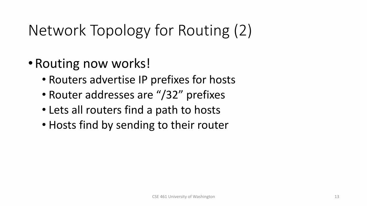
Network Topology for Routing (2)
• Routing now works!• Routers advertise IP prefixes for hosts• Router addresses are “/32” prefixes• Lets all routers find a path to hosts• Hosts find by sending to their router
CSE 461 University of Washington 13
Hierarchical Routing

CSE 461 University of Washington 15
Internet Growth
• At least a billion Internet hosts and growing …

CSE 461 University of Washington 16
Internet Routing Growth
• Internet growth translates into routing table growth (even using prefixes) …
Source: By Mro (Own work), CC-BY-SA-3.0 , via Wikimedia Commons
Year
Nu
mb
er o
f IP
Pre
fixe
s
Ouch!
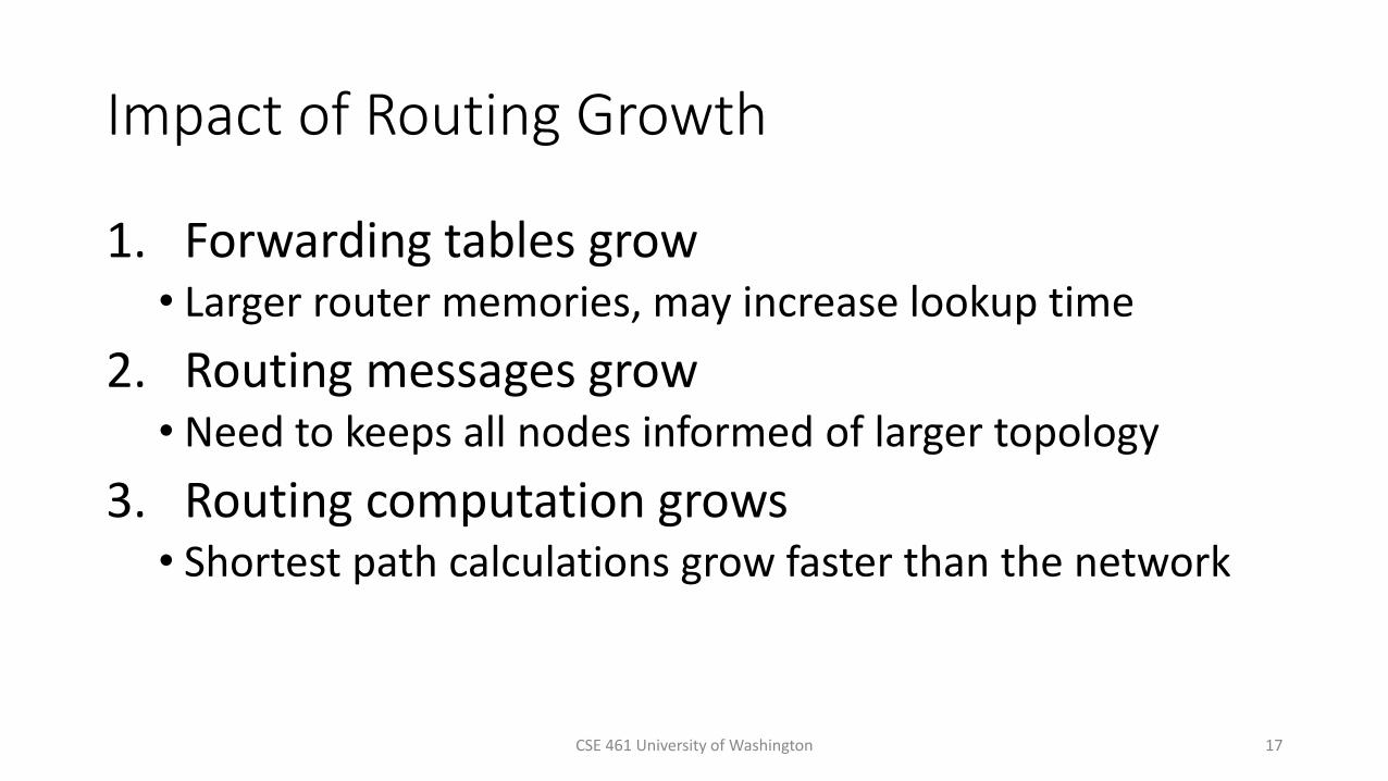
Impact of Routing Growth
1. Forwarding tables grow• Larger router memories, may increase lookup time
2. Routing messages grow• Need to keeps all nodes informed of larger topology
3. Routing computation grows• Shortest path calculations grow faster than the network
CSE 461 University of Washington 17

Techniques to Scale Routing
• First: Network hierarchy• Route to network regions
• Next: IP prefix aggregation• Combine, and split, prefixes
CSE 461 University of Washington 18

Idea
• Scale routing using hierarchy with regions• Route to regions, not individual nodes
CSE 461 University of Washington 19
To the West!
West East
Destination

Hierarchical Routing
• Introduce a larger routing unit• IP prefix (hosts) from one host• Region, e.g., ISP network
• Route first to the region, then to the IP prefix within the region
• Hide details within a region from outside of the region
CSE 461 University of Washington 20

Hierarchical Routing (2)
CSE 461 University of Washington 21

Hierarchical Routing (3)
CSE 461 University of Washington 22
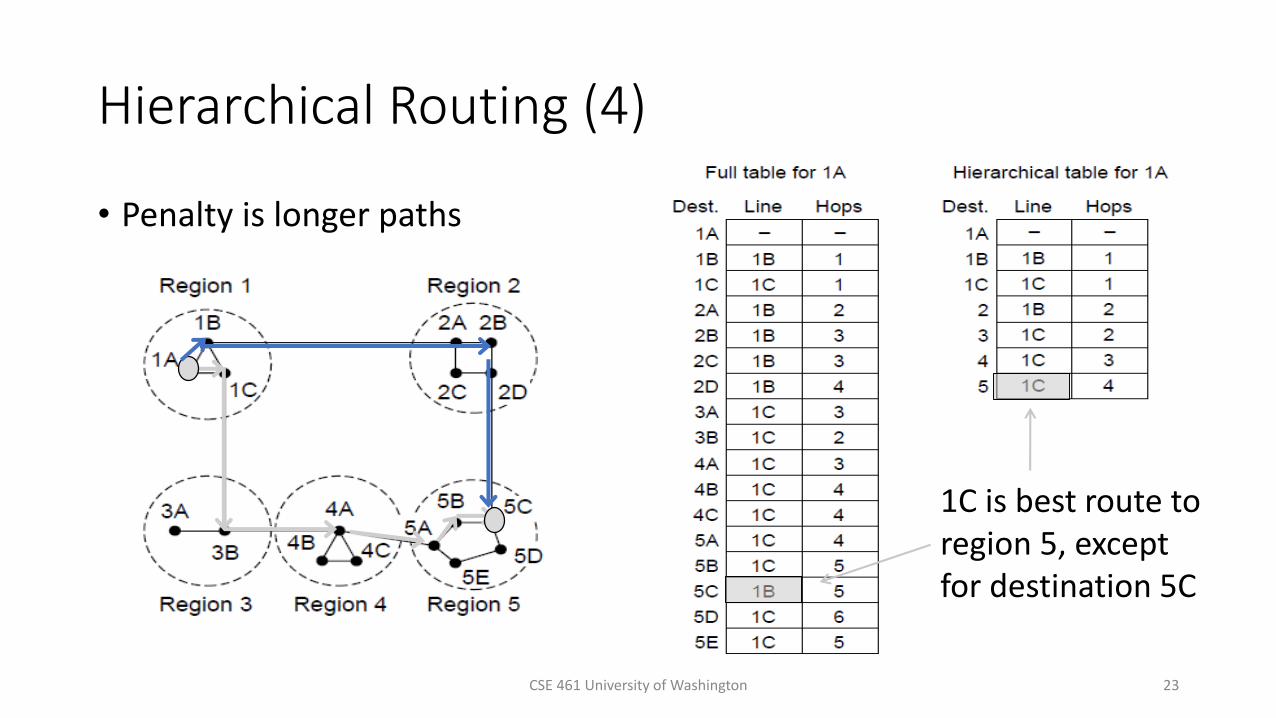
Hierarchical Routing (4)
• Penalty is longer paths
CSE 461 University of Washington 23
1C is best route to region 5, except for destination 5C

Observations
• Outside a region, nodes have one route to all hosts within the region
• This gives savings in table size, messages and computation
• However, each node may have a different route to an outside region
• Routing decisions are still made by individual nodes; there is no single decision made by a region
CSE 461 University of Washington 24

IP Prefix Aggregation and Subnets

Idea
• Scale routing by adjusting the size of IP prefixes• Split (subnets) and join (aggregation)
CSE 461 University of Washington 26
I’m the whole region
Region1
2
3
IP /16IP1 /19
IP2 /18
IP3 /17

Recall
• IP addresses are allocated in blocks called IP prefixes, e.g., 18.31.0.0/16
• Hosts on one network in same prefix
• “/N” prefix has the first N bits fixed and contains 232-N addresses
• E.g., a “/24” has 256 addresses
• Routers keep track of prefix lengths• Use it as part of longest prefix matching
27
Routers can change prefix lengths without affecting hosts
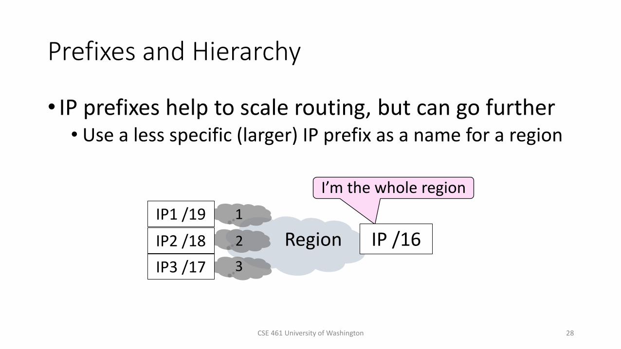
Prefixes and Hierarchy
• IP prefixes help to scale routing, but can go further• Use a less specific (larger) IP prefix as a name for a region
CSE 461 University of Washington 28
I’m the whole region
Region
1
2
3
IP /16
IP1 /19
IP2 /18
IP3 /17
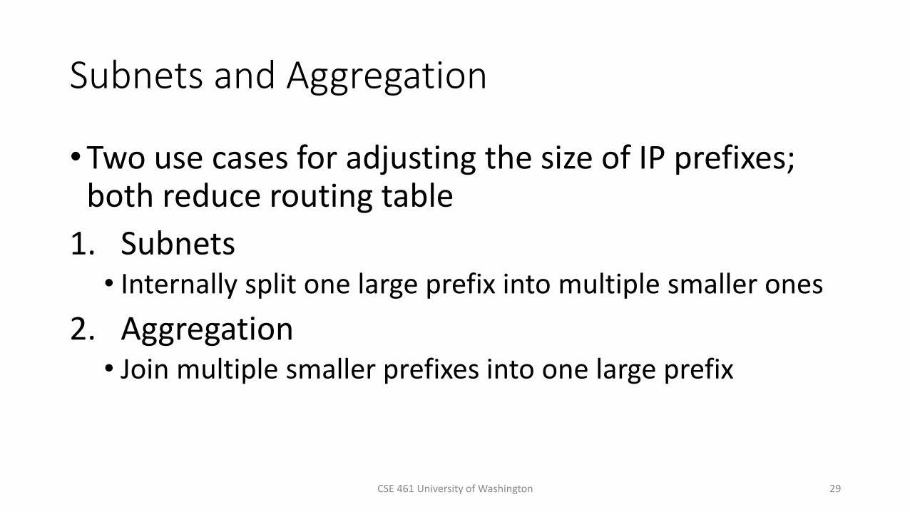
Subnets and Aggregation
• Two use cases for adjusting the size of IP prefixes; both reduce routing table
1. Subnets• Internally split one large prefix into multiple smaller ones
2. Aggregation• Join multiple smaller prefixes into one large prefix
CSE 461 University of Washington 29

Subnets
• Internally split up one IP prefix
32K addresses
One prefix sent to rest of Internet16K
8K
4K Company Rest of Internet

Aggregation
• Externally join multiple separate IP prefixes
One prefix sent to rest of Internet
\
ISPRest of Internet

Routing Process
1. Ship these prefixes or regions around to nearby routers
2. Receive multiple prefixes and the paths of how you got them
3. Build a global routing table

Best Path Routing
CSE 461 University of Washington 34
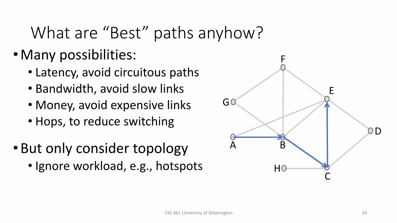
What are “Best” paths anyhow?• Many possibilities:
• Latency, avoid circuitous paths• Bandwidth, avoid slow links• Money, avoid expensive links• Hops, to reduce switching
• But only consider topology• Ignore workload, e.g., hotspots
A B
C
D
E
F
G
H

Shortest Paths
We’ll approximate “best” by a cost function that captures the factors
• Often call lowest “shortest”
1. Assign each link a cost (distance)
2. Define best path between each pair of nodes as the path that has the lowest total cost (or is shortest)
3. Pick randomly to any break ties
CSE 461 University of Washington 35

CSE 461 University of Washington 36
Shortest Paths (2)
• Find the shortest path A E
• All links are bidirectional, with equal costs in each direction
• Can extend model to unequal costs if needed A B
C
D
E
F
G
H
2
1
10
2
2
4
24
4
3
3
3

CSE 461 University of Washington 37
Shortest Paths (3)
• ABCE is a shortest path
• dist(ABCE) = 4 + 2 + 1 = 7
• This is less than:• dist(ABE) = 8• dist(ABFE) = 9• dist(AE) = 10• dist(ABCDE) = 10
A B
C
D
E
F
G
H
2
1
10
2
2
4
24
4
3
3
3

CSE 461 University of Washington 38
Shortest Paths (4)
• Optimality property:• Subpaths of shortest paths are
also shortest paths
• ABCE is a shortest pathSo are ABC, AB, BCE, BC, CE
A B
C
D
E
F
G
H
2
1
10
2
2
4
24
4
3
3
3
CSE 461 University of Washington 39
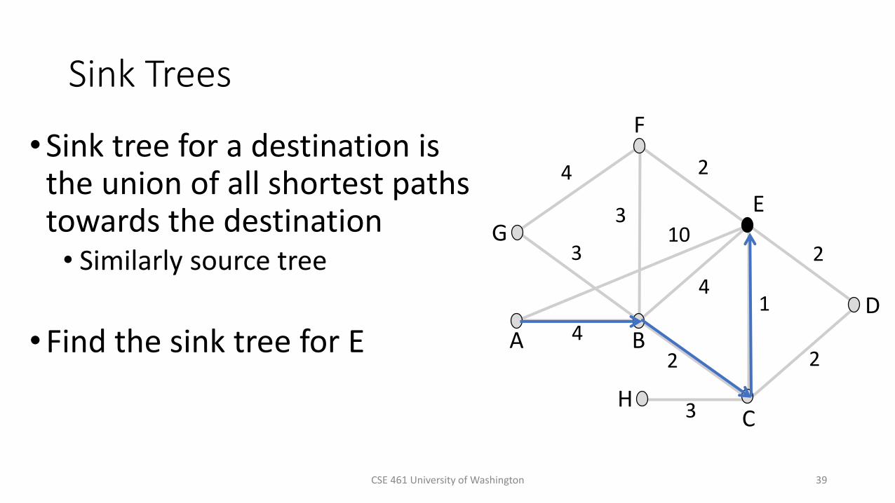
Sink Trees
• Sink tree for a destination is the union of all shortest paths towards the destination
• Similarly source tree
• Find the sink tree for E A B
C
D
E
F
G
H
2
1
10
2
2
4
24
4
3
3
3

CSE 461 University of Washington 40
Sink Trees (2)
• Implications:• Only need to use destination to
follow shortest paths• Each node only need to send to
the next hop
• Forwarding table at a node• Lists next hop for each
destination• Routing table may know more
A B
C
D
E
F
G
H
2
1
10
2
2
4
24
4
3
3
3

Distance Vector Routing
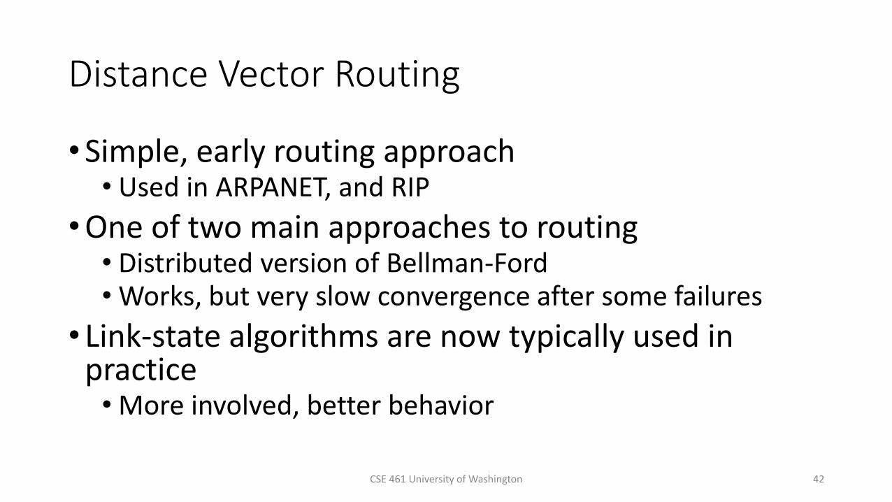
Distance Vector Routing
• Simple, early routing approach• Used in ARPANET, and RIP
• One of two main approaches to routing• Distributed version of Bellman-Ford• Works, but very slow convergence after some failures
• Link-state algorithms are now typically used in practice
• More involved, better behavior
CSE 461 University of Washington 42

Distance Vector Setting
Each node computes its forwarding table in a distributed setting:
1. Nodes know only the cost to their neighbors; not topology
2. Nodes can talk only to their neighbors using messages
3. All nodes run the same algorithm concurrently
4. Nodes and links may fail, messages may be lost
CSE 461 University of Washington 43

Distance Vector Algorithm
Each node maintains a vector of distances (and next hops) to all destinations1. Initialize vector with 0 (zero) cost to self, ∞ (infinity) to
other destinations
2. Periodically send vector to neighbors
3. Update vector for each destination by selecting the shortest distance heard, after adding cost of neighbor link
4. Use the best neighbor for forwarding
CSE 461 University of Washington 44

Distance Vector (2)
• Consider from the point of view of node A• Can only talk to nodes B and E
CSE 461 University of Washington 45
A B
C
D
E
F
G
H
2
1
10
2
2
4
24
4
3
3
3
To Cost
A 0
B ∞
C ∞
D ∞
E ∞
F ∞
G ∞
H ∞
Initialvector

Distance Vector (3)
• First exchange with B, E; learn best 1-hop routes
46
A B
C
D
E
F
G
H
2
1
10
2
2
4
24
4
3
3
3
A’s
Cost
A’s
Next
0 --
4 B
∞ --
∞ --
10 E
∞ --
∞ --
∞ --
ToB
says
E
says
A ∞ ∞
B 0 ∞
C ∞ ∞
D ∞ ∞
E ∞ 0
F ∞ ∞
G ∞ ∞
H ∞ ∞
B
+4
E
+10
∞ ∞
4 ∞
∞ ∞
∞ ∞
∞ 10
∞ ∞
∞ ∞
∞ ∞
Learned better route

Distance Vector (4)
• Second exchange; learn best 2-hop routes
CSE 461 University of Washington 47
A B
C
D
E
F
G
H
2
1
10
2
2
4
24
4
3
3
3
A’s
Cost
A’s
Next
0 --
4 B
6 B
12 E
8 B
7 B
7 B
∞ --
ToB
says
E
says
A 4 10
B 0 4
C 2 1
D ∞ 2
E 4 0
F 3 2
G 3 ∞
H ∞ ∞
B
+4
E
+10
8 20
4 14
6 11
∞ 12
8 10
7 12
7 ∞
∞ ∞

Distance Vector (4)
• Third exchange; learn best 3-hop routes
CSE 461 University of Washington 48
A B
C
D
E
F
G
H
2
1
10
2
2
4
24
4
3
3
3
A’s
Cost
A’s
Next
0 --
4 B
6 B
8 B
7 B
7 B
7 B
9 B
ToB
says
E
says
A 4 8
B 0 3
C 2 1
D 4 2
E 3 0
F 3 2
G 3 6
H 5 4
B
+4
E
+10
8 18
4 13
6 11
8 12
7 10
7 12
7 16
9 14

Distance Vector (5)
• Subsequent exchanges; converged
CSE 461 University of Washington 49
A B
C
D
E
F
G
H
2
1
10
2
2
4
24
4
3
3
3
A’s
Cost
A’s
Next
0 --
4 B
6 B
8 B
8 B
7 B
7 B
9 B
ToB
says
E
says
A 4 7
B 0 3
C 2 1
D 4 2
E 3 0
F 3 2
G 3 6
H 5 4
B
+4
E
+10
8 17
4 13
6 11
8 12
7 10
7 12
7 16
9 14

Distance Vector Dynamics
• Adding routes:• News travels one hop per exchange
• Removing routes:• When a node fails, no more exchanges, other nodes forget
CSE 461 University of Washington 50
Problem?

DV Dynamics (2)
• Good news travels quickly, bad news slowly (inferred)
CSE 461 University of Washington 51
“Count to infinity” scenario
Desired convergence
X

DV Dynamics (3)
• Various heuristics to address• “Split horizon”
• Don’t send route back to where you learned it from. • Poison reverse
• Send “infinity” when you notice a disconnect
• But none are very effective• Link state now favored in practice• Except when very resource-limited
CSE 461 University of Washington 52

RIP (Routing Information Protocol)
• DV protocol with hop count as metric• Infinity is 16 hops; limits network size• Includes split horizon, poison reverse
• Routers send vectors every 30 seconds• Runs on top of UDP• Time-out in 180 secs to detect failures
• RIPv1 specified in RFC1058 (1988)
CSE 461 University of Washington 53
Link-State Routing

Link-State Routing
• Other broad class of routing algorithms• Trades more computation than distance vector for better
dynamics
• Widely used in practice• Used in Internet/ARPANET from 1979• Modern networks use OSPF (L3) and IS-IS (L2)
CSE 461 University of Washington 55
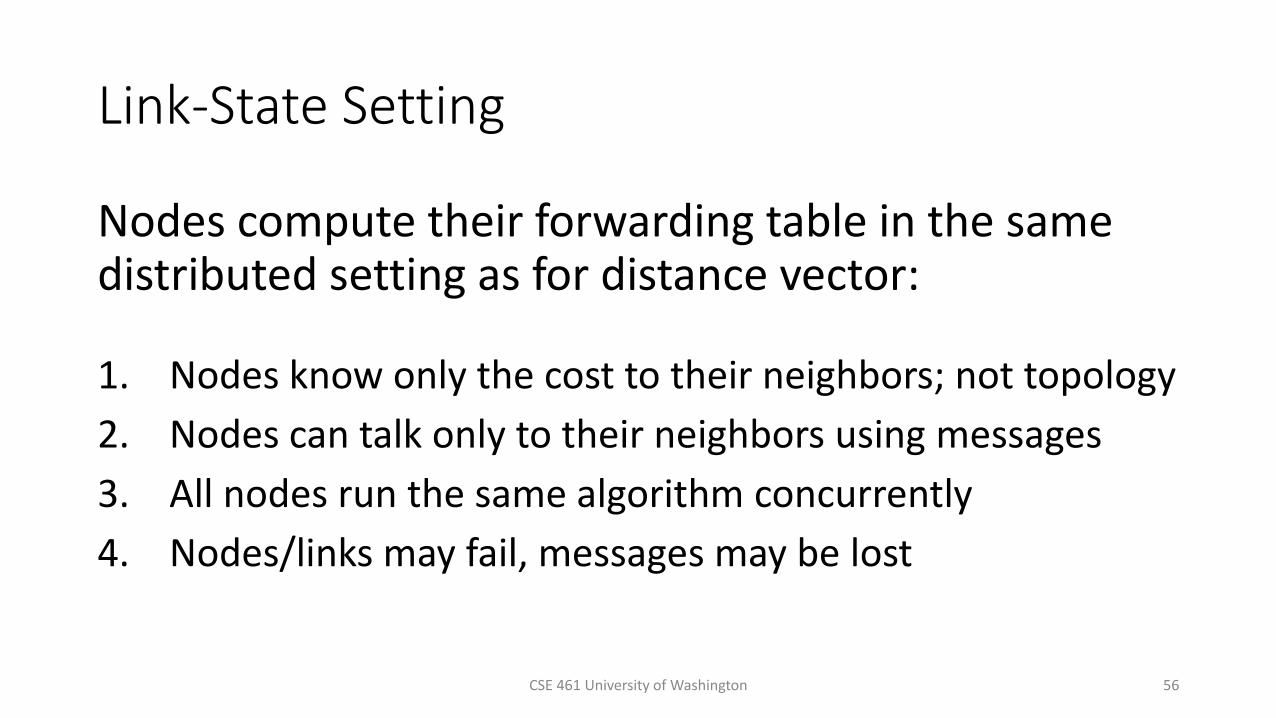
Link-State Setting
Nodes compute their forwarding table in the same distributed setting as for distance vector:
1. Nodes know only the cost to their neighbors; not topology
2. Nodes can talk only to their neighbors using messages
3. All nodes run the same algorithm concurrently
4. Nodes/links may fail, messages may be lost
CSE 461 University of Washington 56

Link-State Algorithm
Proceeds in two phases:
1. Nodes flood topology with link state packets• Each node learns full topology
2. Each node computes its own forwarding table• By running Dijkstra (or equivalent)
CSE 461 University of Washington 57

Part 1: Flood Routing

Flooding
• Rule used at each node:• Sends an incoming message on to all other neighbors• Remember the message so that it is only flood once
CSE 461 University of Washington 59

Flooding (2)
• Consider a flood from A; first reaches B via AB, E via AE
CSE 461 University of Washington 60
A B
C
D
E
F
G
H

Flooding (3)
• Next B floods BC, BE, BF, BG, and E floods EB, EC, ED, EF
CSE 461 University of Washington 61
A B
C
D
E
F
G
H
E and B send to each other

Flooding (4)
• C floods CD, CH; D floods DC; F floods FG; G floods GF
62
A B
C
D
E
F
G
H
F gets another copy

Flooding (5)
• H has no-one to flood … and we’re done
CSE 461 University of Washington 63
A B
C
D
E
F
G
H
Each link carries the message, and in at least one direction

Flooding Details
• Remember message (to stop flood) using source and sequence number
• So next message (with higher sequence) will go through
• To make flooding reliable, use ARQ• So receiver acknowledges, and sender resends if needed
CSE 461 University of Washington 64
Problem?

Flooding Problem
• F receives the same message multiple times
CSE 461 University of Washington 65
A B
C
D
E
F
G
H
E and B send to each other too

Part 2: Dijkstra’s Algorithm

CSE 461 University of Washington 67
Edsger W. Dijkstra (1930-2002)
• Famous computer scientist• Programming languages• Distributed algorithms• Program verification
• Dijkstra’s algorithm, 1969• Single-source shortest paths, given
network with non-negative link costs
By Hamilton Richards, CC-BY-SA-3.0, via Wikimedia Commons
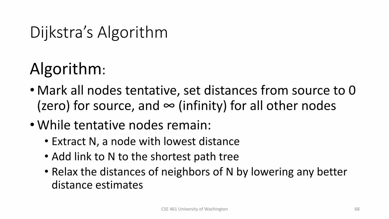
Dijkstra’s Algorithm
Algorithm:
• Mark all nodes tentative, set distances from source to 0 (zero) for source, and ∞ (infinity) for all other nodes
• While tentative nodes remain:• Extract N, a node with lowest distance• Add link to N to the shortest path tree• Relax the distances of neighbors of N by lowering any better
distance estimates
CSE 461 University of Washington 68

Dijkstra’s Algorithm (2)
• Initialization
CSE 461 University of Washington 69
A B
C
D
E
F
G
H
2
1
10
2
2
4
24
4
3
3
3
0 ∞
∞ ∞
∞
∞
∞
We’ll compute shortest paths
from A ∞
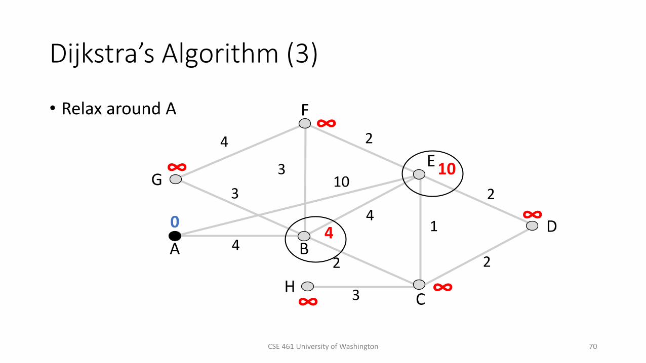
Dijkstra’s Algorithm (3)
• Relax around A
CSE 461 University of Washington 70
A B
C
D
E
F
G
H
2
1
10
2
2
4
24
4
3
3
3
0 ∞
∞ 10
4
∞
∞
∞

Dijkstra’s Algorithm (4)
• Relax around B
CSE 461 University of Washington 71
A B
C
D
E
F
G
H
2
1
10
2
2
4
24
4
3
3
3
0∞
8
4
Distance fell!
6
7
7
∞

Dijkstra’s Algorithm (5)
• Relax around C
CSE 461 University of Washington 72
A B
C
D
E
F
G
H
2
1
10
2
2
4
24
4
3
3
3
0
7
4
Distance fellagain!
6
7
7
8
9
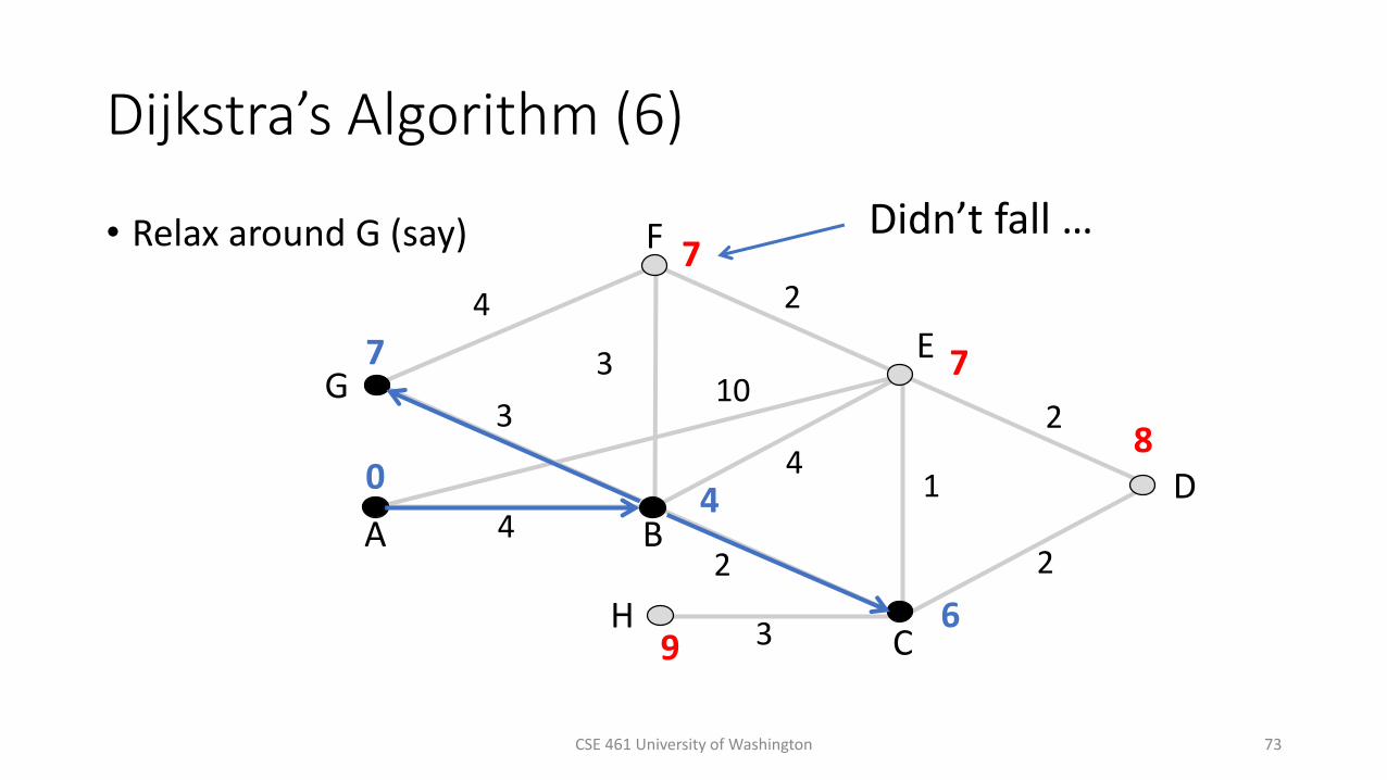
Dijkstra’s Algorithm (6)
• Relax around G (say)
CSE 461 University of Washington 73
A B
C
D
E
F
G
H
2
1
10
2
2
4
24
4
3
3
3
0
7
4
Didn’t fall …
6
7
7
8
9

Dijkstra’s Algorithm (7)
• Relax around F (say)
CSE 461 University of Washington 74
A B
C
D
E
F
G
H
2
1
10
2
2
4
24
4
3
3
3
0
7
4
Relax has no effect
6
7
7
8
9

Dijkstra’s Algorithm (8)
• Relax around E
CSE 461 University of Washington 75
A B
C
D
E
F
G
H
2
1
10
2
2
4
24
4
3
3
3
0
7
4
6
7
7
8
9

Dijkstra’s Algorithm (9)
• Relax around D
CSE 461 University of Washington 76
A B
C
D
E
F
G
H
2
1
10
2
2
4
24
4
3
3
3
0
7
4
6
7
7
8
9

Dijkstra’s Algorithm (10)
• Finally, H … done
CSE 461 University of Washington 77
A B
C
D
E
F
G
H
2
1
10
2
2
4
24
4
3
3
3
0
7
4
6
7
7
8
9

Dijkstra Comments
• Finds shortest paths in order of increasing distance from source
• Leverages optimality property
• Runtime depends on cost of extracting min-cost node• Superlinear in network size (grows fast) • Using Fibonacci Heaps the complexity turns out to be
O(|E|+|V|log| V|)
• Gives complete source/sink tree• More than needed for forwarding!• But requires complete topology
CSE 461 University of Washington 78

Bringing it all together…

CSE 461 University of Washington 80
Phase 1: Topology Dissemination• Each node floods link state packet
(LSP) that describes their portion of the topology
A B
C
D
E
F
G
H
2
1
10
2
2
4
24
4
3
3
3
Seq. #
A 10
B 4
C 1
D 2
F 2
Node E’s LSP flooded to A, B, C, D, and F

Phase 2: Route Computation
• Each node has full topology• By combining all LSPs
• Each node simply runs Dijkstra• Replicated computation, but finds required routes directly• Compile forwarding table from sink/source tree• That’s it folks!
CSE 461 University of Washington 81

Forwarding Table
CSE 461 University of Washington 82
To Next
A C
B C
C C
D D
E --
F F
G F
H CA B
C
D
E
F
G
H
2
1
10
2
2
4
24
4
3
3
3
Source Tree for E (from Dijkstra) E’s Forwarding Table

Handling Changes
• On change, flood updated LSPs, re-compute routes• E.g., nodes adjacent to failed link or node initiate
CSE 461 University of Washington 83
A B
C
D
E
F
G
H
2
1
10
2
24
24
4
3
3
3
XXXXSeq. #
A 4
C 2
E 4
F 3
G ∞
B’s LSPSeq. #
B 3
E 2
G ∞
F’s LSPFailure!

Handling Changes (2)
• Link failure• Both nodes notice, send updated LSPs• Link is removed from topology
• Node failure• All neighbors notice a link has failed• Failed node can’t update its own LSP• But it is OK: all links to node removed
CSE 461 University of Washington 84

Handling Changes (3)
• Addition of a link or node• Add LSP of new node to topology• Old LSPs are updated with new link
• Additions are the easy case …
CSE 461 University of Washington 85

Link-State Complications
• Things that can go wrong:• Seq. number reaches max, or is corrupted• Node crashes and loses seq. number• Network partitions then heals
• Strategy:• Include age on LSPs and forget old information that is not
refreshed
• Much of the complexity is due to handling corner cases
CSE 461 University of Washington 86

DV/LS Comparison
CSE 461 University of Washington 87
Goal Distance Vector Link-State
Correctness Distributed Bellman-Ford Replicated Dijkstra
Efficient paths Approx. with shortest paths Approx. with shortest paths
Fair paths Approx. with shortest paths Approx. with shortest paths
Fast convergence Slow – many exchanges Fast – flood and compute
Scalability Excellent – storage/compute Moderate – storage/compute

IS-IS and OSPF Protocols
• Widely used in large enterprise and ISP networks• IS-IS = Intermediate System to Intermediate System• OSPF = Open Shortest Path First
• Link-state protocol with many added features• E.g., “Areas” for scalability
CSE 461 University of Washington 88

Equal-Cost Multi-Path Routing

Multipath Routing
• Allow multiple routing paths from node to destination be used at once
• Topology has them for redundancy• Using them can improve performance
• Questions:• How do we find multiple paths?• How do we send traffic along them?
CSE 461 University of Washington 90

CSE 461 University of Washington 91
Equal-Cost Multipath Routes• One form of multipath routing
• Extends shortest path model by keeping set if there are ties
• Consider AE• ABE = 4 + 4 = 8• ABCE = 4 + 2 + 2 = 8• ABCDE = 4 + 2 + 1 + 1 = 8• Use them all!
A B
C
D
E
F
G
H
2
2
10
1
1
4
24
4
3
3
3

Source “Trees”
• With ECMP, source/sink “tree” is a directed acyclic graph (DAG)
• Each node has set of next hops• Still a compact representation
CSE 461 University of Washington 92
Tree DAG
CSE 461 University of Washington 93
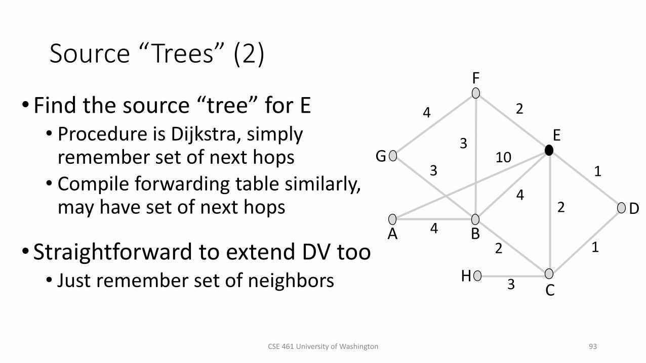
Source “Trees” (2)
• Find the source “tree” for E• Procedure is Dijkstra, simply
remember set of next hops• Compile forwarding table similarly,
may have set of next hops
• Straightforward to extend DV too• Just remember set of neighbors
A B
C
D
E
F
G
H
2
2
10
1
1
4
24
4
3
3
3

Source “Trees” (3)
CSE 461 University of Washington 94
Source Tree for E E’s Forwarding Table
A B
C
D
E
F
G
H
2
2
10
1
1
4
24
4
3
3
3
Node Next hops
A B, C, D
B B, C, D
C C, D
D D
E --
F F
G F
H C, D
New for ECMP

Forwarding with ECMP
• Could randomly pick a next hop for each packet based on destination
• Balances load, but adds jitter
• Instead, try to send packets from a given source/destination pair on the same path
• Source/destination pair is called a flow• Map flow identifier to single next hop• No jitter within flow, but less balanced
CSE 461 University of Washington 95

Forwarding with ECMP (2)
CSE 461 University of Washington 96
A B
C
D
E
F
G
H
2
2
10
1
1
4
24
4
3
3
3
Multipath routes from F/E to C/H E’s Forwarding Choices
FlowPossible
next hops
Example
choice
F H C, D D
F C C, D D
E H C, D C
E C C, D C
Use both paths to getto one destination

Border Gateway Protocol (BGP)

Structure of the Internet
• Networks (ISPs, CDNs, etc.) group with IP prefixes• Networks are richly interconnected, often using IXPs
CDN C
Prefix C1
ISP A
Prefix A1
Prefix A2Net F
Prefix F1
IXPIXP
IXPIXP
CDN D
Prefix D1
Net E
Prefix E1
Prefix E2
ISP B
Prefix B1
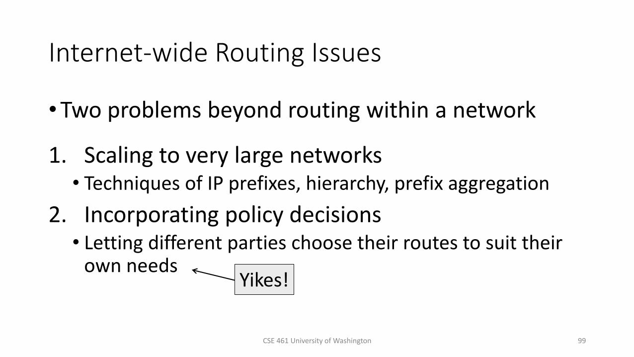
Internet-wide Routing Issues
• Two problems beyond routing within a network
1. Scaling to very large networks• Techniques of IP prefixes, hierarchy, prefix aggregation
2. Incorporating policy decisions• Letting different parties choose their routes to suit their
own needs
CSE 461 University of Washington 99
Yikes!

CSE 461 University of Washington 100
Effects of Independent Parties
• Each party selects routes to suit its own interests
• e.g, shortest path in ISP
• What path will be chosen for A2B1 and B1A2?
• What is the best path? Prefix B2
Prefix A1
ISP A ISP B
Prefix B1
Prefix A2

CSE 461 University of Washington 101
Effects of Independent Parties (2)
• Selected paths are longer than overall shortest path
• And symmetric too!
• This is a consequence of independent goals and decisions, not hierarchy
Prefix B2
Prefix A1
ISP A ISP B
Prefix B1
Prefix A2

Routing Policies
• Capture the goals of different parties• Could be anything• E.g., Internet2 only carries non-commercial traffic
• Common policies we’ll look at:• ISPs give TRANSIT service to customers• ISPs give PEER service to each other
CSE 461 University of Washington 102

CSE 461 University of Washington 103
Routing Policies – Transit• One party (customer) gets TRANSIT
service from another party (ISP)• ISP accepts traffic for customer from
the rest of Internet• ISP sends traffic from customer to the
rest of Internet• Customer pays ISP for the privilege
Customer 1
ISP
Customer 2
Rest ofInternet
Non-customer

CSE 461 University of Washington 104
Routing Policies – Peer• Both party (ISPs in example) get
PEER service from each other• Each ISP accepts traffic from the other
ISP only for their customers• ISPs do not carry traffic to the rest of
the Internet for each other• ISPs don’t pay each other
Customer A1
ISP A
Customer A2
Customer B1
ISP B
Customer B2

Routing with BGP (Border Gateway Protocol)
• iBGP is for internal routing
• eBGP is interdomain routing for the Internet• Path vector, a kind of distance vector
105
ISP APrefix A1
Prefix A2Net F
Prefix F1
IXP
ISP BPrefix B1 Prefix F1 via ISP
B, Net F at IXP

Routing with BGP (2)
• Parties like ISPs are called AS (Autonomous Systems)• AS numbers assigned by regional Internet Assigned
Numbers Authority (IANA) like APNIC• AS’s MANUALLY configure their internal BGP
routes/advertisements• External routes go through complicated filters for
forwarding/filtering• AS BGP routers communicate with each other to
keep consistent routing rules
CSE 461 University of Washington 106

Routing with BGP (2)
•Border routers of ASes announce BGP routes
•Route announcements have IP prefix, path vector, next hop• Path vector is list of ASes on the way to the prefix• List is to find loops
•Route announcements move in the opposite direction to traffic
CSE 461 University of Washington 107

Routing with BGP (3)
CSE 461 University of Washington 108
Prefix

Routing with BGP (4)
Policy is implemented in two ways:
1. Border routers of ISP announce paths only to other parties who may use those paths
• Filter out paths others can’t use
2. Border routers of ISP select the best path of the ones they hear in any, non-shortest way
CSE 461 University of Washington 109
Routing with BGP (5)
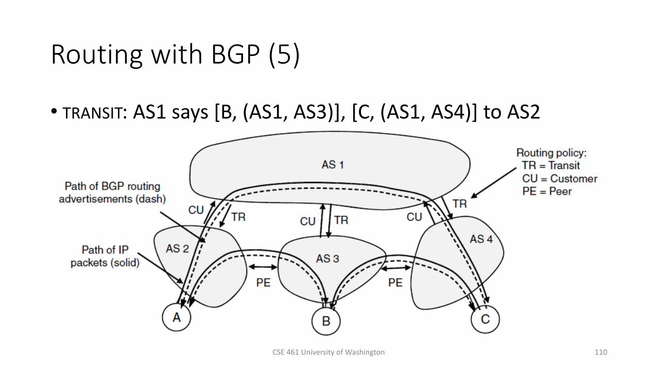
• TRANSIT: AS1 says [B, (AS1, AS3)], [C, (AS1, AS4)] to AS2
CSE 461 University of Washington 110

Routing with BGP (6)
• CUSTOMER (other side of TRANSIT): AS2 says [A, (AS2)] to AS1
CSE 461 University of Washington 111

Routing with BGP (7)
• PEER: AS2 says [A, (AS2)] to AS3, AS3 says [B, (AS3)] to AS2
CSE 461 University of Washington 112

Routing with BGP (8)
• AS2 has two routes to B (AS1, AS3) and chooses AS3 (Free!)
CSE 461 University of Washington 113


BGP Thoughts
• Much more beyond basics to explore!• Policy is a substantial factor
• Can independent decisions be sensible overall?
• Other important factors:• Convergence effects• How well it scales• Integration with intradomain routing• And more …
CSE 461 University of Washington 115
Cellular Routing
Addressing in Cellular
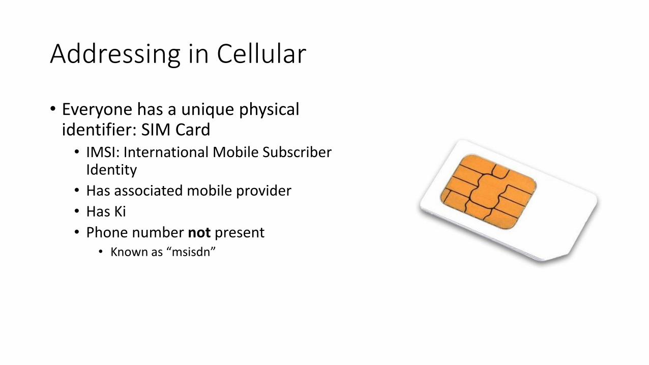
• Everyone has a unique physical identifier: SIM Card
• IMSI: International Mobile Subscriber Identity
• Has associated mobile provider
• Has Ki
• Phone number not present• Known as “msisdn”

Cellular Core Networks

In-network routing
1. User dials phone number
2. Number is “looked up” in some database
3. If local, we get the associated IMSI
4. Check that sender and send and receiver can receive
5. Look up tower group of IMSIs last registration
6. Page the receiver
7. Bill them both

Out-of-network Routing
• Signaling System No. 7 (SS7)• Performs number translation, local number portability,
prepaid billing, Short Message Service (SMS), roaming, and other stuff
• Either directly connected or connected through aggregators such as Cybase
• Business vs Protocols

Cellular Lookups
• An SSP telephone exchange receives a call to an 0800 number. This causes a trigger within the SSP that causes an SCP (Service Control Point) to be queried using SS7 protocols (INAP, TCAP). The SCP responds with a geographic number, e.g. 0121 XXX XXXX, and the call is actually routed to a phone.
