sensors

Article

A Hybrid Spectral Clustering and Deep NeuralNetwork Ensemble Algorithm for Intrusion Detectionin Sensor NetworksTao Ma 1,2, Fen Wang 2, Jianjun Cheng 1, Yang Yu 1 and Xiaoyun Chen 1,*

1 School of Information Science and Engineering, Lanzhou University, Lanzhou 730000, China;matlzu@163.com (T.M.); chengjianjun@lzu.edu.cn (J.C.); yuyang_1102@163.com (Y.Y.)

2 School of Mathematical and Computer Science, Ningxia Normal University, Guyuan 756000, China;wangfen_2015@163.com

* Correspondence: chenxy@lzu.edu.cn; Tel.: +86-136-0931-9826

Academic Editors: Muhammad Imran, Athanasios V. Vasilakos, Thaier Hayajneh and Neal N. XiongReceived: 26 July 2016; Accepted: 8 October 2016; Published: 13 October 2016

Abstract: The development of intrusion detection systems (IDS) that are adapted to allow routers andnetwork defence systems to detect malicious network traffic disguised as network protocols or normalaccess is a critical challenge. This paper proposes a novel approach called SCDNN, which combinesspectral clustering (SC) and deep neural network (DNN) algorithms. First, the dataset is divided intok subsets based on sample similarity using cluster centres, as in SC. Next, the distance between datapoints in a testing set and the training set is measured based on similarity features and is fed into thedeep neural network algorithm for intrusion detection. Six KDD-Cup99 and NSL-KDD datasets anda sensor network dataset were employed to test the performance of the model. These experimentalresults indicate that the SCDNN classifier not only performs better than backpropagation neuralnetwork (BPNN), support vector machine (SVM), random forest (RF) and Bayes tree models indetection accuracy and the types of abnormal attacks found. It also provides an effective tool of studyand analysis of intrusion detection in large networks.

Keywords: intrusion detection system; deep neural network; ensemble model; wireless sensornetwork; spectral clustering

1. Introduction

Networking has become ubiquitous in people’s lives and work; hence, network security bearsincreasing importance for network users and operators. Network intrusion detection is a networksecurity mechanism designed to detect, prevent and repel unauthorized access to a communicationor computer network. IDSs play a crucial role in maintaining safe and secure networks. In recentyears, vast amounts of network data have been generated due to the application of new networktechnologies and equipment, which has led to declining detection rates. The intrusion detectionprocess is complicated due to the dynamic nature of networks and the power available for processinghigh volumes of data from distrusted network systems, making it difficult to achieve high detectionaccuracy at rapid speeds [1].

Many researchers have proposed innovative approaches to intrusion detection in recent years.These methods, based on detecting behaviour and access resource type, are divided into four categories.The first uses statistical analysis to detect attack types based the relationships between nodes ina network, such as with Bayesian [2], decision tree and fuzzy logic models. These techniques buildmodels of normal network data and calculate the probability that a given sample deviates fromthese models. If the probability that a sample value’s deviation is greater than threshold, then thesample is classified as a type of attack [3]. The second category is an anomaly detection approach

Sensors 2016, 16, 1701; doi:10.3390/s16101701 www.mdpi.com/journal/sensors

Sensors 2016, 16, 1701 2 of 23

in which most methods require a set of standard normal datasets to train a classifier and determinewhether new samples fit the model. Examples of such methods include SC, self-organizing map (SOM)and unsupervised support vector machine approaches [4]. The third category employs classificationtechniques to detect attack types by taking advantage of machine learning algorithms such as SVM [5],RFs [6], genetic algorithms (GA) and artificial neural networks (ANN), which can prioritize solutions tocertain problems. The last category includes hybrid and ensemble detection methods that integrate theadvantages of various methods in order to increase detection accuracy [7]. These approaches includebagging, AdaBoost [8], and the Particle Swarm Optimization (PSO)-K-means ensemble approach [9].The PSO-k-means method can achieve an optimal number of clusters, as well as increasing detectionrates while decreasing false positive rate, and can be successful in detecting network intrusion.In addition, the SVM-KNN-PSO ensemble method proposed by [10] can obtain the best results.However this work is based on binary classification methods, which can distinguish between onlytwo states.

Recently, deep learning has become a popular topic of research, and methods based on deeplearning have successfully been widely applied in image identification and speech recognition.In recent literature, deep learning has been used in network security detection. The self-taught learning(STL) model, based on deep learning techniques, was proposed for network intrusion detection.This model utilized a sparse auto-encoder (SAE) to learn dataset features; the NSL-KDD datasetwas used to test its detection performance [11]. Deep belief networks (DBN) are used to initialisethe parameters of DNN through a pre-training process. Initialising a DNN with probability-basedfeature vectors is used to detect vehicular networks and significantly improves detection rates [12].Fiore et al. [13] proposed a novel model for network anomaly detection based on a semi-superviseddiscriminative restricted Boltzmann machine (DRBM), which decouples training and generalizes theneural networks. In a previous hybrid model, Salama et al. [14] proposed a combination of a DBNand SVM. The DBN is used to reduce the dimensionality of the input dataset and the SVM is used toclassify attack types.

For complicated network attacks, some research has focused on rule-based expert detection,which utilizes pre-designed processing rules to detect attacks [15]; however, for very large datasets,rule-based expert approaches become less capable. Additionally, wireless sensor networks (WSN),a new post-Internet network architecture, are widely and increasingly used in a variety of smartenvironment applications. Adding these to conventional and mobile networks, and taking intoconsideration the diverse intrusion methods available to malicious agents, the technical requirementsof intrusion detection are more complex than ever before [16]. Attacks on WSNs are easier to carry outthan those on wired networks because the distribution of WSNs is inherently limited, and because ofthe multi-hop communication, bandwidth and battery power used therein. Therefore, designingan effective IDS for WSNs is very important. Due to this new environment, new attacks havebeen devised (e.g., black hole, sink hole, abnormal transmission and packet dropping attacks). Theattacks are divided by mechanism into signature, anomaly and hybrid intrusion detection methods.The anomaly detection method, for instance, is widely used for security in WSNs [17].

However, intrusion detection has been insufficient in several ways. First, the learning capacity oftraditional detection approaches that sum features of the raw data, map them into vectors, and thenfeed them to a classifier is limited. When network structure is complicated, learning efficiencyfurther decreases. Second, this primary method only partially represents one or two levels ofinformation; it is insufficient for identifying additional attack types. Third, in real network datasets,the types of network intrusion are similar to those in normal datasets, which confine classifiersfrom having enough information with which to categorize them. Next, the intrusion actions behaveunpredictably, which causes IDS to make costly errors in detecting intrusions. Therefore, it is necessaryto find an effective intrusion detection method [18]. Finally, the variety of network types has generatedlarge-scale data with high-dimensional structures, for which traditional intrusion detection approachesare unsuitable [19].

Sensors 2016, 16, 1701 3 of 23

Literature concerning fields in which many-layered learners represent network dataset featuresis quite limited. Lin et al. [20] proposed combining the k-means and k-Nearest Neighbour(KNN) algorithms to select dataset features and to categories network attack types. Samples arereconstructed into clusters and a two-dimensional vector dataset is generated with different features.Then, the training dataset is divided into subsets by the KNN algorithm. This approach more efficientlydetects normal data and Denial of service (DoS) attacks with high accuracy, but it does not performwell in detecting user-to-root (U2R) and remote-to-local (R2L) attacks, which means that the selectedfeatures represent these attack types poorly and the proposed model can only learn limited patterns.

Taking the above into consideration, this paper proposes the SCDNN model, which uses spectralclustering to capture raw data features and divide the dataset into subsets. Each subset is then fedto a DNN. These DNNs can learn information about different characteristics of the subset. The testdatasets have previously been divided by training dataset features into subsets. Finally, the test subsetsare fed to the trained DNN for intrusion detection. Because the SC algorithm can extract similarfeatures and acquire more information from a dataset, the DNN can obtain sufficient information viaprior learning, which enables the DNN to familiarize itself with as many of the rules and features ofnetwork attack types as possible. Deep learning is believed to be able to extract features from massiveand complex datasets; hence, it can solve non-linear problems with complex and large-scale data(e.g., it has been applied in weather forecasting) [21,22]. Experimental results based on the KDD-CUP99dataset and NLS-KDD datasets show that an SCDNN generates better accuracy and more robust resultsthan other well-known algorithms, and excels in parallel computing [23–26].

The contribution of this study is as follows: First, we adopt SC to capture the features of complexnetwork datasets, for attack types similar to normal access, using clustering to find features thatdivide the dataset into subsets with different cluster centres. Second, taking advantage of multi-layerDNNs, attack types can be learned at high, abstract levels of network data and complex networkintrusion rules can be found. The intrusion process is becoming more variable and easily disguisedas normal network activity. This situation is particularly common in large datasets and complicatesthe relationship between distributed processing protocols. Knowledge of categories in a dataset issufficient for the SCDNN model to be able to learn. Finally, our experimental results indicate that theaccuracy, detection and false alarm rates of SCDNN are better than those of conventional methods.

The rest of the paper is organized as follows. The related literature concerning IDS is reviewed inSection 2. Section 3 presents a detailed definition of the proposed approach and describes how thealgorithm works. Section 4 describes the experimental dataset and illustrates the data preparation,evaluation criteria, results and discussions of experiments. Finally, the conclusions and suggestions forfuture work are provided in Section 5.

2. Related Works

In this section, the spectral clustering and DNN algorithms are briefly introduced. To overcome thelimitations of traditional auto-encoders, this study adapts a SAE and denoising auto-encoders (DAEs)for the DNN. IDSs are a classification problem in which dataset features are very important, because thelearner acquires knowledge and patterns based on the characteristics of the data. Additionally, thelevel of feature representation determines a learner’s performance.

2.1. Spectral Clustering Algorithm

Spectral clustering uses the top eigenvectors of a matrix derived from the input data andtransforms the clustering problem into a graph cut problem. The graph cutting approach clustersdata points by attribute such that densely packed points are in same cluster, whereas the sparse are indifferent clusters. The minimum cut formula is written as:

cut(x, y) = ∑i∈A,j∈B Wij (1)

Sensors 2016, 16, 1701 4 of 23

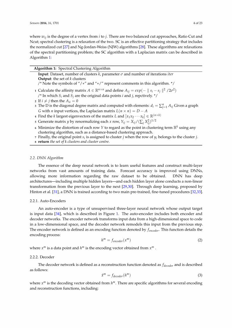
where wij is the degree of a vertex from i to j. There are two balanced cut approaches, Ratio Cut andNcut; spectral clustering is a relaxation of the two. SC is an effective partitioning strategy that includesthe normalized cut [27] and Ng-Jordan-Weiss (NJW) algorithms [28]. These algorithms are relaxationsof the spectral partitioning problem; the SC algorithm with a Laplacian matrix can be described inAlgorithm 1:

Algorithm 1: Spectral Clustering AlgorithmInput: Dataset, number of clusters k, parameter σ and number of iterations iterOutput: the set of k clusters/* Note the symbols of “/∗” and “∗/” represent comments in this algorithm. */

1 Calculate the affinity matrix A ∈ Rn×n and define Aij = exp(− ‖ si − sj ‖2 /2σ2)

/* In which Si and Sj are the original data points i and j, repctively. */2 If i 6= j then the Aii = 03 The D is the diagonal degree matrix and computed with elements: di = ∑n

j=1 Aij Given a graphG with n input vertices, the Laplacian matrix L(n× n) = D− A

4 Find the k largest eigenvectors of the matrix L and [x1x2 · · · xk] ∈ R(n×k)

5 Generate matrix y by renormalizing each x row, Yij = Xij/(∑j X2ij)

1/2

6 Minimize the distortion of each row Y to regard as the point in clustering term Rk using anyclustering algorithm, such as a distance-based clustering approach.

7 Finally, the original point si is assigned to cluster j when the row of yi belongs to the cluster j.8 return the set of k clusters and cluster centre.

2.2. DNN Algorithm

The essence of the deep neural network is to learn useful features and construct multi-layernetworks from vast amounts of training data. Forecast accuracy is improved using DNNs,allowing more information regarding the raw dataset to be obtained. DNN has deeparchitectures—including multiple hidden layers—and each hidden layer alone conducts a non-lineartransformation from the previous layer to the next [29,30]. Through deep learning, proposed byHinton et al. [31], a DNN is trained according to two main pre-trained, fine-tuned procedures [32,33].

2.2.1. Auto-Encoders

An auto-encoder is a type of unsupervised three-layer neural network whose output targetis input data [34], which is described in Figure 1. The auto-encoder includes both encoder anddecoder networks. The encoder network transforms input data from a high-dimensional space to codein a low-dimensional space, and the decoder network remodels this input from the previous step.The encoder network is defined as an encoding function denoted by fencoder. This function details theencoding process:

hm = fencoder(xm) (2)

where xm is a data point and hm is the encoding vector obtained from xm .

2.2.2. Decoder

The decoder network is defined as a reconstruction function denoted as fdecoder and is describedas follows:

x̂m = fdecoder(hm) (3)

where xm is the decoding vector obtained from hm. There are specific algorithms for several encodingand reconstruction functions, including:

Sensors 2016, 16, 1701 5 of 23

Logsig : fencoder(xm) =1

1 + e−xm (4)

Satline : fencoder(xm) =

0 i f xm ≤ 0z i f 0 < xm < 11 i f xm ≥ 1

(5)

Pureline : fencoder(xm) = xm (6)

encoder decoder

input dataoutput data

1

mx

2

mx

m

nx

1̂

mx

2ˆmx

ˆm

nx

mh

Figure 1. Architecture of an auto-encoder and decoder in a deep neural network (DNN).

2.2.3. Sparse Auto-Encoder (SAE)

The default auto-encoder attempts to learn feature approximation, and the function of theauto-encoder of x′ is close to the raw input data of x. It is seems that the identity function is able tolearn most features of the input data. However, the number of units in each layer of the neural networkis constrained, with x′ as the minimum original size. When the number of hidden units increases,runtime efficiency decreases for the analysis of input data features, although the auto-encoder will stilllearn the features of the raw data. From the above analysis, a sparsity coder can constrain the inputdata with useful identification information [35]. Let a(2)j (x) represent the activation of the jth hiddenunits by the auto-encoder from the input x, so that the average activation of the jth unit in the hiddenlayer is defined as follows [36]:

ρ̂j =1m

m

∑i=1

[a(2)j (x(i))] (7)

Averaged over the input set, let ρ̂j represent the degree of sparsity, where ρ is a sparsity parameter.Let ρ̂j = ρ, which is a small value close to 0; typically, the value of ρ is set to 0.05. To satisfy thecondition that the activation is near 0, a penalty term is added to optimise the deviation of ρ̂j from ρ.The optimisation formula is defined as follows:

s2

∑j=1

ρlogρ

ρ̂j+ (1− ρ)log

1− ρ

1− ρ̂j(8)

in which the number of hidden-layer units is s2 and j denotes hidden units in the network.The Kullback-Leibler (KL) divergence is written as follows [37]:

s2

∑j=1

KL(ρ ‖ ρ̂j) (9)

where the KL divergence between a Bernoulli random variable with a mean of ρ and ρ̂j is definedas below:

Sensors 2016, 16, 1701 6 of 23

KL(ρ ‖ ρ̂j) = ρlogρ

ρ̂j+ (1− ρ)log

1− ρ

1− ρ̂j(10)

If ρ̂j equals ρ, then the value of Equation (9) is equal to 0, which means that the KL divergencereaches the minimum value and close to 0, so the overall cost function is defined as follows:

Jsparse(W, b) = J(W, b) + βs2

∑j=1

KL(ρ ‖ ρ̂j) (11)

where J(w, b) is the squared error cost function and defined as:

Jsparse(W, b) =

[1m

m

∑i=1

J(w, b; x(i), y(i))

]+

λ

2

nl−1

∑l=1

sl

∑i=1

sl+1

∑j=1

(W(l)ji )2 (12)

The first term of the function J(W, b) is an average sum of squared error over m samplesand outputs. The second term is a weight decay term which can decrease the magnitude of each weightin a neural network and can effectively prevent overfitting. From Equation (11), β is a coefficient toadjust the weight of the sparsity penalty term. The term ρ̂j depends on the neural network parametersW and b, and it is optimised using a derivative checking method [38]. The stochastic gradient descent(SGD) approach is adopted to optimise W and b, and can be written as follows:

Wij(l) = Wij(l)− ε∂

∂Wij(l)Csparse(W, b) (13)

bi(l) = bi(l)− ε∂

∂bi(l)Csparse(W, b) (14)

in Equations (13) and (14), ε is the learning rate; squared errors are obtained by training over examplesand calculating the average ρ̂j. The best values of W and b are obtained by back propagation with SGD.

2.2.4. Denoising Auto-Encoders (DAEs)

There is a way to capture something useful about the hidden units with input data. DAEs are usedto discover more robust hidden-layer features and can effectively prevent the networks from simplylearning features. The DAE is a stochastic auto-encoder that tries to represent information about theinput data that can only be learned by capturing the statistical attributes between the encoded andinput data. The DAEs can be represented in a variety of ways, including from stochastic operator,bottom-up-information and top-down-generative model perspectives. In this paper, the DAEs learnedfeature representations by adjusting partial corruption from the input pattern [39]. A fixed number ofcomponents in each input x(i) are chosen randomly and their value set to zero; this distribution iscalled qD(·), then the joint distribution of input and output is defined as follows:

q0(X, χ, y) = q0(X)qD(χ|X)δ fθ(χ)(y) (15)

in which the encoding of X is a stochastic mapping by the distribution χ ∼ qD(χ|X). If the conditionfθ(x) 6= y · q0(X) is satisfied, then δ fθ(χ)

(y) indicates the empirical distribution associated with theinput data and set to 0. χ can be determined by y. In order to obtain the best reconstructed version ofX′ with consideration between χ and y, let θ be a parameter of the joint distribution of Equation (15),and calculate the minimum error of the cost function of the input matrix X from y as follows:

arg minθ,θ′

Eq0(X,χ)[L(X, X′)] (16)

Sensors 2016, 16, 1701 7 of 23

where [L(X, X′)] is the error function depending on input x and the reconstructed X′. The best costfunction value is then obtained using SGD. To encode optimised denoising codes, there is a trickin encoder process. Let y be a hidden representation obtained with the function sigmoid(Wχ + b),where χ is a generated corrupted version of the input data and the parameters of the function aredenoted as θ = {W, b}. Each corrupted code contains some elements of input X randomly set to 0.Then, the final corrupted version can be minimised in Equation (16).

2.2.5. Pre-Training

N auto-encoders can be stacked to pre-train an N-hidden-layer DNN. When given an inputdataset, the input layer and the first hidden layer of the DNN are treated as the encoder network ofthe first auto-encoder. Next, the first auto-encoder is trained by minimising its reconstruction error.The trained parameter set of the encoder network is used to initialise the first hidden layer of the DNN.Then, the first and second hidden layers of the DNN are regarded as the encoder network of thesecond auto-encoder. Accordingly, the second hidden layer of the DNN is initialised by the secondtrained auto-encoder. This process proceeds until the Nth auto-encoder is trained to initialise thefinal hidden layer of the DNN. Thus, all hidden layers of the DNN are stacked in an auto-encoderin each training N times, and are regarded as pre-trained. This pre-training process is proven to besignificantly better than random initialisation of the DNN and conducive to achieving generalisationin classification [40,41].

2.2.6. Fine-Tuning

Fine-tuning is a supervised process that improves the performance of a DNN. The network isretrained, training data are labelled, and errors calculated by the difference between real and predictedvalues are back-propagated using SGD for all multi-layer networks. SGD randomly selects datasetsamples and iteratively updates the gradient direction with weight parameters. The best gradientdirection is obtained with a minimum loss function. The advantage of SGD is that it converges fasterthan the traditional gradient descent methods do, and does not consider the entire dataset, making itsuitable for complex neural networks. The SGD equation is defined below:

E =12 ∑

j=1M(yi − ti)

2 (17)

where E is the loss function, y is the real label and t is the network output. The gradient of weightparameter w is obtained by the derivative of the error equation.

∂E∂wij

=∂E∂yj·

∂yj

∂uj·

∂uj

∂wij(18)

With the gradient of wij, the updated SGD equation is defined as:

wnewij = wold

ij − η · (yj − tj) · yj(1− yj) · hi (19)

where η is the step size and is greater than 0, and h is the number of hidden layers in the DNN [42].This process is tuned and optimised by the weight and threshold based on the correctly labelled datain the DNNs. In this way, the DNN can learn important knowledge for its final output and direct theparameters of the entire network to perform correct classifications [43].

3. The Proposed Approach of SCDNN

Several classification engines (BPNN, SVM, RF, Bayes and DNN) perform well given theadvantages of their algorithms, which can efficiently handle complex classification problems;hence, these models can be successfully applied to intrusion detection. They usually perform

Sensors 2016, 16, 1701 8 of 23

poorly when facing the complex randomness and camouflage of network intrusion dataflow.Therefore, in this section, the proposed approach is employed to solve the above problems. First, thetraining data subsets divide the training process and calculate centre points by SC from eachtraining point. Second, each training data subset is trained by the corresponding DNNs, where thescale of DNNs is the same as the number of clusters. In this way, the DNNs have learned differentcharacteristics from each subset. Third, the testing data subsets are divided into test datasets by SC,which uses the previous cluster centres in its first step, and these subsets are applied to detect intrusionattack types by pre-trained DNNs. Finally, the output of every DNN is aggregated for the final resultof the intrusion detection classifiers.

3.1. SCDNN

The SCDNN model includes three steps, and the general task in each step is described as followsand shown in Figure 2.

StageⅠ

t1 t2 tk...

output

1 2 kC C CL

d1 d2 dk...

traindataset

featurecluster

Spectral clustering

testdataset

aggregate

The testing sub datasets areobtained from the testingdataset, which were completedby the training data subsetskin Stage 1.

StageⅡ

Stage Ⅲ

...softmax

22exp( 2 )

ij i jA s s s= - -

( )L n n D - A´ =

2 1/2/ ( )ij ij ijjY X X= å

These testing sub datasetsare applied to detectintrusion attack types.

Dataset 1 Dataset 2 Dataset 3 Dataset 4 Dataset 5 Dataset 6

Data sets

0

20

40

60

80

100

Av

era

ge

accu

racy

(%

)

SVM BPNN RF Bayes SCDNN

softmax

Figure 2. The SCDNN flow chart is divided into three steps and shows each process in detail.

Step 1: The dataset is divided into two components: training and testing datasets. The trainingdataset is clustered by SC and this output is regarded as the training subset labelled Training Datasets1–k. The SC centres from the training dataset clustering process are stored to serve as initialisationcluster centre for generating the testing dataset clusters. Because intrusion data features indicate

Sensors 2016, 16, 1701 9 of 23

similar attributes of each type in the raw dataset, points in the training dataset with similar featuresare aligned into groups and regarded as the same subset. In order to improve SCDNN performance,different cluster numbers and values of sigma are considered. The number of clusters ranged from 2to 6 and sigma from 0.1 to 1.0. The samples are assigned to one cluster by similarity. The minimumdistance from a data point to each cluster centre is measured by Algorithm 1 and each point is assignedto a cluster. The training subsets generated by clusters are given as input to the DNNs. In order to trainthe different subsets, the number of DNNs is equal to the number of data subsets. The architectureof each DNN consists of five layers: two hidden layers, one input layer, one softmax layer and oneoutput layer. In this paper, the two hidden layers learn features from each training subset and thetop layer is a five-dimensional output vector. Each training subset which are generated from thekth cluster centre by SC algorithm in clustering process, regarded as input data to feed into the kthDNN, respectively. These trained sub-DNN models are marked as sub-DNN 1 through sub-DNN k.

Step 2: The testing dataset, which has been divided from the raw dataset, is used to generatek datasets. The previous cluster centres obtained from SC cluster in Step 1, are regarded as theinitialization cluster centres of the SC algorithm in this step. The test dataset which are divided by SCcluster, are regarded testing subsets. These subsets are denoted as Test 1 through Test k.

Step 3: The k testing data subsets are fed into k sub-DNNs, which were completed by the k trainingdata subsets in Step 1. The output of each sub-DNN is integrated as the final output and employed toanalyse positive detection rates. Then, a confusion matrix is used to analyse the detection performanceof the five classifications: Normal, DoS, Probe, U2R and R2L.

3.2. The SCDNN Algorithm

The SCDNN algorithm adopts a deep learning approach to categorise network attack types andfine-tune its weights and thresholds using backpropagation. The input vectors map low-dimensionalspace with DAEs and SAE to discover patterns in the data. The SCDNN algorithm is detailed inAlgorithm 2.

Algorithm 2: SCDNNInput: dataset, cluster number, number of hidden-layer nodes HLN, number of hidden layers HL.Output: Final prediction results/*Note the symbols of “/∗” and “∗/” represent comments in this algorithm.*/

1 Divide the raw dataset into two components: a training dataset and a testing dataset./*get the largest matrix eigenvectors and training data subsets*/

2 Obtain the cluster centres and SC results using Algorithm 1. Here, the clustering results are regarded as training datasubsets./*Train each DNN with each training data subset*/

3 The learning rate, denoising and sparsity parameters are set and the weight and bias are randomly initialised.4 The HL are set two hidden layers, HLN is set 40 nodes of the first hidden layer and 20 nodes of second hidden layer.5 Compute the sparsity cost function Jsparse(W, b) = J(W, b) + β ∑s2

j=1 KL(ρ ‖ ρ̂j).

6 Parameter weights and bias are updated as Wij(l) = Wij(l)− ε∂

∂Wij(l)Csparse(W, b) and

bi(l) = bi(l)− ε ∂∂bi(l)

Csparse(W, b).

7 Train k sub-DNNs corresponding to the training data subsets.8 Fine-tune the sub-DNNs by using backpropagation to train them.9 The final structure of the trained sub-DNNs is obtained and they are labelled with each training data subset.

10 Divide the testing dataset into subsets with SC. Cluster centre parameters from the training data clusters are used.11 The testing data subsets are used to test corresponding sub-DNNs, based on each corresponding cluster centre

between the testing and training data subsets./*aggregate each prediction result*/

12 Results are generated by each sub-DNN, are integrated and the final outputs are obtained.13 return classification result = final output

Sensors 2016, 16, 1701 10 of 23

The eigenvectors of the point matrix and training dataset are generated by the SC output inLines 1–2, the k DNNs are trained in Lines 3–9, the testing data subsets are obtained by calculatingdistance with the NJW algorithm in Line 10, the testing data subsets are used to test the DNNs, and thefinal results are predicted by the aggregation in Lines 11–13.

4. Experimental Results

These experiments examine and compare SCDNNs with other detection models: SVMs, BPNNs,RFs and Bayes. Six datasets from the KDD-CUP99 and NSL-KDD are used to evaluate the performanceof all models. Then, the parameters, number of cluster and DNN weights are discussed and analysed.

4.1. Evaluation Methods

In this study, accuracy, recall, error rate (ER) and specificity are used to evaluate the performanceof the detection models. The formulas of the above criteria are calculated as follows [44]:

Accuracy =TP + TN

TP + TN + FP + FN(20)

Recall =TP

TP + FN(21)

ErrorRate =FP + FN

FP + TP + TN + FN(22)

SPEC =TN

TN + FP(23)

A true positive (TP) is a case that correctly distinguishes network attack type, a true negative(TN) shows normal network data classified correctly as normal, a false negative (FN) denotes a case inwhich an attack was classified as normal dataflow, and a false positive (FP) means that the a normalcase was classified as an attack. The accuracy rate shows the overall correct detection accuracy of thedataset, ER refers to the robustness of the classifier, recall indicates the degree of correctly detectedattack types of all cases classified as attacks, and specificity shows the percentage of correctly classifiednormal data. In the above, higher accuracy and recall and lower ER indicate good performance.

4.2. The Dataset

To evaluate the performance of our proposed approach, a series of experiments on theKDD-CUP-99 [31] and NLS-KDD datasets [22] were conducted. The 10% knowledge KDD-CUP-99datasets are used in these experiments, as it is most comprehensive dataset that is widely usedas a benchmark for the performance intrusion detection network models. Each record contains41-dimensional feature data that of various continuous, discrete and symbolic type. This is unsuitablefor network data records because it includes four attack categories (DoS, probe, R2L and U2R) [45].

In order to solve the above problem, pre-trained data are processed in three steps. First, the valuesof three symbolic features are mapped as a series of numeric values ranging from 1 to N, where Nis the total number of symbols for each feature. Second, the KDD’99 dataset includes five classes,normal, DoS, probe, U2R, and R2L, which were mapped onto the numeric values 1–5, respectively [46].Finally, because of the range of values of field columns of src_bytes and dst_bytes are quite different,in order to find more patterns and more easily handle the proposed method, the range of valuesof these two fields are mapped onto 0–5000. After data pre-processing, the total number of datasetfeatures was transformed to 65.

The NLS-KDD dataset includes the KDDTrain+, KDDTest+ and KDDTest-21 subsets, whichare used for this experiment because the KDD-CUP-99 datasets contain more frequent and harmfulattack records. The NLS-KDD dataset has removed surplus records and is more suitable to evaluatingthe real-world performance of an intrusion detection algorithm. In order to fairly compare the

Sensors 2016, 16, 1701 11 of 23

capability of each algorithm, six datasets were randomly generated from the two KDD-CUP-99 andNSL-KDD datasets, which reduces the amount of data [47]. These are labelled Datasets 1 through 6.Probe, U2R and R2L attack classes occur with low frequency in the raw dataset, so these three typeswere manually distributed, whereas normal and DoS records were randomly selected based on threescales with 1%, 5% and 10% of total in the KDD-CUP-99 dataset, labelled Dataset 1–3, respectively [48].

For the NLS-KDD dataset, the three data subsets are generated from two training and two testingsets and designated Datasets 4–6. The training sets randomly selected 20% and 50% of the raw dataset,and the testing sets are KDDTest+ and KDDTest-21, respectively. Table 1 describes the six new datasetsin detail. The training data of the six datasets include 24 attack types, and the testing data contain38 attack types. Therefore, the test dataset includes specific attack types which are not presented inthe training dataset, which is closer to the actual condition of network intrusion. In this way, we canevaluate the ability of each model to find new attack types.

Table 1. The distribution of the training and testing sets from the six datasets generated from KDD’99and NSL-KDD.

DatasetTraining Dataset Testing Dataset

Normal% DoS% Probe% U2R% R2L% Normal% DoS% Probe% U2R% R2L%

Dataset 1 17.96 72.28 7.583 0.096 2.079 19.48 73.90 1.339 0.073 5.205Dataset 2 19.48 78.40 1.645 0.021 0.451 19.48 73.90 1.339 0.073 5.205Dataset 3 19.69 79.23 0.831 0.011 0.228 19.48 73.90 1.339 0.073 5.205Dataset 4 53.38 36.65 9.086 0.044 0.860 43.07 33.08 10.73 0.887 12.21Dataset 5 48.56 33.11 16.81 0.075 1.435 43.07 33.08 10.73 0.887 12.21Dataset 6 53.38 36.65 9.086 0.044 0.830 18.16 36.64 20.27 1.688 23.24

The six new datasets are used to evaluate the performance of the SCDNN and to compare it tothe other detection methods previously mentioned. In addition, these experiments evaluate modelperformance for one of the novel network architectures arising in today’s networking environment,such as ad hoc wireless networks, WSNs and wireless mesh networks. These networks have developedrapidly and are easier to attack than wired networks. In order to determine the detection performanceof the proposed model in WSNs, the following experiments were carried out [49].

4.3. SCDNN Experiment I

In this section, the number of clusters k in SCDNN is evaluated on the six datasets, because thevalues of k and σ (a parameter of SC), are different in each dataset. k and σ have a serious impact onthe precision of SCDNN results. Next, the testing datasets are used to compare the performance of theremaining five models.

4.3.1. Efficiency of Varied Cluster Numbers and Values of σ

The SCDNN algorithm is composed of three steps. First is clustering the training dataset;the numbers of clusters k ranges from 2 to 6, and the value range of σ in the SC algorithm is 0.1to 1.0. The training data subsets are divided based on the values of k and σ. Different parametersimpact the experiment results. In order to obtain the best efficiency, the average detection accuracyrate of the SCDNN is determined for the six datasets. These results are shown in Figure 3.

Sensors 2016, 16, 1701 12 of 23

0.1 0.2 0.3 0.4 0.5 0.6 0.7 0.8 0.9 1.0

sigma(a)

60

70

80

90

100

Acc

urac

y (%

)

K=2 K=3 K=4 K=5 K=6

0.1 0.2 0.3 0.4 0.5 0.6 0.7 0.8 0.9 1.0

sigma(b)

75

80

85

90

95

100

Acc

urac

y (%

)0.1 0.2 0.3 0.4 0.5 0.6 0.7 0.8 0.9 1.0

sigma(c)

75

80

85

90

95

100

Acc

urac

y (%

)

0.1 0.2 0.3 0.4 0.5 0.6 0.7 0.8 0.9 1.0

sigma(d)

50

60

70

80

90

Acc

urac

y (%

)

0.1 0.2 0.3 0.4 0.5 0.6 0.7 0.8 0.9 1.0

sigma(e)

50

60

70

80

Acc

urac

y (%

)

0.1 0.2 0.3 0.4 0.5 0.6 0.7 0.8 0.9 1.0

sigma(f)

20

30

40

50

Acc

urac

y (%

)

Figure 3. (a–f) Comparing SCDNN accuracy over several cluster numbers k and σ values for thesix datasets.

Figure 3a–f shows testing results from the six datasets obtained from different values of k and σ.For almost all datasets, SCDNN performs best when σ is between 0.4 and 0.5; likewise, the optimalvalue of k is between 2 and 5. In order to clearly explain the testing selection process, the bestparameters for the five attack types in each dataset are shown in Figure 4.

SCDNN prediction accuracy of the five network intrusion types with optimum σ values arehighly volatile with increasing values of k in all datasets. A high k value can efficiently improveSCDNN accuracy; more clusters can be divided into smaller data subsets, which damages the integrityof the input data features and leads to poor SCDNN performance. U2R and R2L attacks comprisea small proportion of the dataset, which prevents the classifier from learning enough information andcauses unbalanced dataset categories. Cluster number can determine how well the particular featuresof underrepresented attack types are mined; therefore, it is necessary to strikes a balance between thenumber of cluster and efficiency. The optimal values of k for each dataset (that is, those with the bestSCDNN accuracy) are presented in Table 2.

Sensors 2016, 16, 1701 13 of 23

2 3 4 5 6

(a) K

sigma=0.5

0

20

40

60

80

100

Acc

ura

cy (

%)

Normal Dos Probe U2R R2L

2 3 4 5 6

(b) K

sigma=0.4

0

20

40

60

80

100

Acc

ura

cy (

%)

2 3 4 5 6

(c) K

sigma=0.5

0

20

40

60

80

100

Acc

ura

cy (

%)

2 3 4 5 6

(d) K

sigma=0.4

0

20

40

60

80

100

Acc

ura

cy (

%)

2 3 4 5 6

(e) K

sigma=0.4

0

20

40

60

80

100

Acc

ura

cy (

%)

2 3 4 5 6

(f) K

sigma=0.5

0

20

40

60

80

100

Acc

ura

cy (

%)

Figure 4. (a–f) Comparing SCDNN accuracy for different numbers of clusters k for the six datasets.

Table 2. Detection accuracy of five attack types using the optimal number of clusters for each dataset.

Dataset k σ Nor (%) DoS (%) Probe (%) U2R (%) R2L (%) Accuracy (%)

Dataset 1 k = 2 0.5 97.21 96.87 80.32 11.4 6.88 91.97Dataset 2 k = 4 0.4 98.42 97.2 70.64 3.51 1.57 92.03Dataset 3 k = 5 0.5 97.61 97.23 65.96 4.39 6.59 92.1Dataset 4 k = 3 0.4 96.17 75.84 53.37 3.00 3.01 72.64Dataset 5 k = 3 0.4 97.19 74.51 48.37 5.00 0.62 71.83Dataset 6 k = 5 0.5 84.20 50.02 52.66 1.50 0.98 44.55

Figures 3 and 4 and Table 2 show that accuracy rates are volatile when k is less than 4, while greatstability can be obtained when k is greater than 5. The best results occur when k is set to 2 in Dataset 1,with an overall accuracy of 91.97% and high DoS, probe and R2L detection rates. This implies that theclustering process can be classified into normal and attack types, which helps the SCDNN maintainefficient network intrusion categories. In the same way, the best results occur when k is 4, 5, 3 and3 in Datasets 2 to 5, respectively. The total accuracy is 44.55% in the Dataset 6 when k is set to 5.

Sensors 2016, 16, 1701 14 of 23

Accuracy is low across attack types because attack features are similar to those of normal data and arehard to detect. U2R and R2L attack detection results in low accuracy in all datasets except Dataset 1,probably because there are few such records in the dataset and their features are similar to those ofDoS and probe attacks, which provides the DNN with less information and causes increased detectionrate errors.

4.3.2. Results and Comparisons

In this section, the fusion matrix and evaluation criteria are calculated for the SCDNN and thefour traditional detection methods for each of the six datasets. The optimal cluster number k andσ value are fed into each DNN described in Section 3. The DNNs have 65 input dimensions andfive output dimensions, because the original dataset is a 65-dimensional vector and the goal is todistinguish five intrusion attack types. There are two hidden layers, the first has 40 neurons and thesecond has 20. The softmax layer has five dimensions. 10% validation is used to check for overfittingduring the training process. The results of the above experiment are shown in Table 3 and Figure 5.

Table 3. Comparing network intrusion detection results for the six datasets (%).

Dataset Model Normal DoS Probe U2R R2L Acc Recall ER

Dataset 1

SVM 98.21 83 66.01 0.88 3.14 81.52 77.72 18.48BP 96.51 89.49 46.18 9.21 1.93 85.66 83.48 14.34RF 93.65 96.62 59.27 0 0 90.44 91.08 9.56

Bayes 91.51 95.59 61.35 4.39 3.56 89.48 92.57 10.52SCDNN 97.21 96.87 80.32 11.4 6.88 91.97 91.68 8.03

Dataset 2

SVM 96.22 97.1 65.84 0 0.05 91.39 90.52 8.61BP 91.44 97.42 62.69 7.02 5.41 90.93 92.88 9.07RF 98.23 96.48 38.26 0 0 90.95 89.51 9.05

Bayes 95.92 95.98 62.55 4.82 4.38 90.69 91.07 9.31SCDNN 98.42 97.2 70.64 3.51 1.57 92.03 91.35 7.97

Dataset 3

SVM 95.87 97.23 64.86 0 0.06 91.41 90.59 8.59BP 81.53 96.95 8.81 6.14 7.26 88.03 90.05 11.97RF 99.57 96.57 0 0 0 90.76 89.37 9.24

Bayes 96.38 96.29 59.15 7.02 7.46 91.12 90.95 8.88SCDNN 97.61 97.23 65.96 4.39 6.59 92.1 92.23 7.9

Dataset 4

SVM 95.54 70.18 57.37 0 1.63 70.73 53.26 29.27BP 96.35 71.17 65.55 0 0.58 72.16 57.79 27.84RF 99.63 63.11 7.23 0 0 64.57 40.45 35.43

Bayes 93.9 72.18 41.02 0 0 68.73 52.78 31.27SCDNN 96.17 75.84 53.37 3 3.01 72.64 57.48 27.36

Dataset 5

SVM 98.57 18.93 49.89 0 0.11 54.1 20.45 45.9BP 91.79 7.63 66.58 1.5 2.43 49.53 27.56 50.47RF 99.69 62.64 48.99 0 0 68.93 46.43 31.07

Bayes 99.06 61.65 35.4 0 0 66.87 44.28 33.13SCDNN 97.19 74.51 48.37 5 0.62 71.83 55.08 28.17

Dataset 6

SVM 95.81 41.5 43.67 0 0 41.46 30.6 58.54BP 74.72 4.61 88.67 0 1.53 33.59 30.6 66.41RF 99.72 36.15 6.74 0 0 32.73 18.9 67.27

Bayes 82.16 48.25 28.52 0 0 38.37 30.08 61.63SCDNN 84.2 50.02 52.66 1.5 0.98 44.55 37.85 55.45

The records are unbalanced in each of the six datasets; Normal and DoS cases are well-represented,whereas U2R and R2L occur rarely, because the latter two cases require complex intrusion actionsgenerally carried out by an advanced user, resulting in more covert intrusion that is difficult to detect.

From Table 3 and Figure 5, considering overall accuracy, the SCDNN performs better than theother four methods and has the lowest error rates. Moreover, the proposed method shows especiallygood performance for the sparse U2R and R2L attack types in all datasets, and produces a higheraccuracy rate than the other methods. The best accuracy rate for Dataset 1 is 98.21%, obtained by SVM.The SCDNN achieves 97.21% accuracy for normal data, proving that the SVM has better learned the

Sensors 2016, 16, 1701 15 of 23

features of the data than other models. All methods are effective for intrusion detection with thisdataset, except for the RF method, which has low precision and 0% detection accuracy for U2R andR2L attack types. For Dataset 2, the SCDNN attains higher precision for normal, DoS and probe traffic,with rates of 98.42%, 97.20% and 70.64%, respectively, and lower precision for U2R and R2L trafficthan the BPNN. In this experiment the BPNN results in higher recall than other methods for the sparseattack types, which illustrates that the BPNN, with simple layer, has obtained the expected accuracy ina specific dataset, though its performance is unstable. The RF algorithm performs well for the morecommon traffic, but obtained 0% accuracy in detecting cases of U2R and R2L attacks. It may be thatthe construction of the trees used by this method can effectively classify most data, but some sparseattack types belong to false classes.

Normal Dos Probe U2R R2L

(a) Dataset 1

0

20

40

60

80

100

Acc

ura

cy (

%)

SVM BPNN RF Bayes SCDNN

Normal Dos Probe U2R R2L

(b) Dataset 2

0

20

40

60

80

100

Acc

ura

cy (

%)

Normal Dos Probe U2R R2L

(c) Dataset 3

0

20

40

60

80

100

Acc

ura

cy (

%)

Normal Dos Probe U2R R2L

(d) Dataset 4

0

20

40

60

80

100

Acc

ura

cy (

%)

Normal Dos Probe U2R R2L

(e) Dataset 5

0

20

40

60

80

100

Acc

ura

cy (

%)

Normal Dos Probe U2R R2L

(f) Dataset 6

0

20

40

60

80

100

Acc

ura

cy (

%)

Figure 5. (a–f) Prediction accuracy histogram of the five detection models.

In Dataset 3, the SCDNN performs best on DoS and probe intrusions, with precision rates of97.23% and 64.96%, respectively. This result indicates that the proposed method is robust and captures

Sensors 2016, 16, 1701 16 of 23

most patterns in the different datasets; in addition, the Bayes model has the highest rates, 7.02% and7.46%, respectively, for the U2R data among all methods. The traditional machine learning models,RF and SVM, produce good results for normal and DoS data. BPNNs, RFs and the SCDNN show goodand effective detection rates for normal, DoS and probe data in Datasets 4 and 5; the RF has the highestaccuracies, 99.63% and 99.69%, of detecting normal traffic in the two datasets, though the SCDNNproduced higher accuracy for DoS data and is effective in detecting sparse attack types. The RF, SVMand Bayes methods performed poorly in classifying rare attack types, with accuracy rates close to 0%.

Overall precision of all methods is quite low for Dataset 6, although the SCDNN performs betterthan other methods in overall accuracy and recall. Specifically, the RF has the highest accuracy rate,99.72%, for normal data; the precision of the BPNN for probe traffic is 88.67%, significantly better thanthe second highest rate, 52.66%, produced by the SCDNN. One potential explanation for this differenceis that the BPNN learns enough patterns from the dataset to detect this kind of attack type. In summary,the SCDNN is good at detecting probe intrusions and the sparse attack types, U2R and R2L. It obtainshigh overall accuracy and recall; however, the SVM, BP, RF and Bayes methods can serve for detectingnormal traffic and DoS data. Especially, the RF is excellent in capturing the normal class, producingthe highest accuracy rates in Datasets 3–6. These results show that DNNs are robust and capable ofdetecting sparse attack classes and can locate new attack types, which further proves that SCDNN aremore suitable for intrusion detection.

The architecture of the proposed model is a hybrid of spectral clustering technology anddeep neural networks. SC clusters samples by their features, an unsupervised process that canclassify unknown attack type. Therefore, clustering can find patterns hidden in the samples basedtheir attributes. In Experiment 1, SC is used to divide the dataset; initial groups are obtained usingsample attributes. In this way, each sub-DNN is trained with special datasets obtained in the clusteringprocess, and have found more information than they would otherwise, because the DNN model hasmore layers than the other, shallower models and used SAE to resample the raw dataset. The questionof the number of hidden layer to use in the DNN is more complicated, as the DAEs increasescomputational overhead and finds more robust features in hidden layers. As shown in Table 1,the five attacks types are imbalanced. The last three attack types are the rarest. Their features areobtained by the data subsets generated by the clustering stage. This can help the SCDNN learn morefeatures of sparse attack types. According to Table 3, the SCDNN performs well in detecting sparseattacks types: probe, U2R and R2L.

4.4. SCDNN Experiment II with a WSN Dataset

In order to test the performance of SCDNN for maintaining the security of WSNs, in thisexperiment the all-in-one (ns-2) network simulator platform is used to generate a test dataset.Because WSNs are widely used in industry and their multi-hop, distributed nature differs fromthat of exit networks, external intrusion in WSNs has become a popular topic of research in academia.Various kinds of security attack cases increase with the number of sensor nodes in a WSN. Therefore,it is important to adopt the proposed method to detect intrusion attacks in WSNs.

In this experiment, there are 10 to 50 sensor nodes to simulate attacker datasets; the ad hocon-demand distance vector (AODV) protocol is assigned in each nodes. The sensor nodes transportprotocol with a constrained bit rate and generated at a random time. The simulated platform generatesa dataset which include protocol messages and data messages. For convenience, the dataset is adaptedfor the proposed algorithm; synthetic data are labelled with security attack types based on knownmajor attack types on the AODV protocol and are shown in Table 4 [50,51].

Sensors 2016, 16, 1701 17 of 23

Table 4. Basic attacker types with packet routing protocols on the ad hoc on-demand distance vector(AODV) protocol in wireless sensor networks (WSNs).

Attack Name Attack Description Attack Type

Active Reply The route reply is forged with abnormal support to reply. 1Route drop The routing packets are dropped with some specific address. 2Modify Sequence The number of target sequences increases with largest maximal values. 3Rushing Rushing of routing messages. 4Data Interruption A data packet is used to drop the route. 5Route Modification The route is modified in Routing Table Entries. 6Change Hop The route cost in routing tables entries is altered. 7

There are seven attack types that can be categorized based on consideration of their protocolmessages in term of message type, transfer time and the number of hops. In this experiment,the detection methods are run 500 times each and the average detection accuracy if given as thefinal result. The output results are shown in Table 5.

Table 5. Average detection accuracy for five sensor nodes scales by the SCDNN algorithm usingoptimal k and sigma values (%).

Dataset ParameterSensor Nodes

10 Nodes 20 Nodes 30 Nodes 40 Nodes 50 Nodes

5% Attacker in Networksk = 4, σ = 0.1 96.8 96.4 95.8 94.5 94.6k = 4, σ = 0.5 93.1 93.5 92.4 89.3 88.7k = 4, σ = 1.0 89.6 89.2 86.5 82.4 83.3

10% Attacker in Networksk = 4, σ = 0.1 96.8 96.4 95.8 94.5 94.6k = 4, σ = 0.5 93.1 93.5 92.4 89.3 88.7k = 4, σ = 1.0 89.6 89.2 86.5 82.4 83.3

The detection accuracy at each sensor node scale is shown in Figure 6 and Table 5. The SCDNNcan detect all seven attack types with high detection rates. For the 5% attack scale, the proposed modelcan find almost all attackers. Detection rates decrease with increasing the size of the attacker to 10%in the network. Moreover, detection accuracy is impacted for different values of σ. The reason forthis change may be that when the attack process attempts to modify router information, the resultingincrease of transport packets in WSNs makes detection performance more unstable.

10 20 30 40 50

sensor nodes

70

75

80

85

90

95

100

Acc

urac

y (%

)

5% attackers in networks

SCDNN sigma=0.1

SCDNN sigma=0.5

SCDNN sigma=1.0

10 20 30 40 50

sensor nodes

70

75

80

85

90

95

100

Acc

urac

y (1

0%)

10% attackers in networks

SCDNN sigma=0.1SCDNN sigma=0.5SCDNN sigma=1.0

(a) (b)

Figure 6. Detection accuracy with five sensor node scales with 95% confidence interval. Accuracy isshown for (a) a 5% attacker and (b) a 10% attacker, 500 times each.

Sensors 2016, 16, 1701 18 of 23

5. Discussion

In order to evaluate the performance of the SCDNN and compare it with the experimental resultsof the other four models in this section, receiver operating curves (ROC) are obtained for all models [52].The ROC function is widely used to indicate an algorithm’s discriminative capability in this field.The overall category performance of each model, the true positive rate (TPR) from Equation (11) andthe false positive rate (FPR) (calculated as 1-Specificity from Equation (13)) are used to generate theROC in Figure 7.

0 0.2 0.4 0.6 0.8 1

FPR

(a) Dataset 1

0

0.2

0.4

0.6

0.8

1

TP

R

SVM BP RF Bayes SCDNN

0 0.2 0.4 0.6 0.8 1

FPR

(b) Dataset 2

0

0.2

0.4

0.6

0.8

1

TP

R

0 0.2 0.4 0.6 0.8 1

FPR

(c) Dataset 3

0

0.2

0.4

0.6

0.8

1

TP

R

0 0.2 0.4 0.6 0.8 1

FPR

(d) Dataset 4

0

0.2

0.4

0.6

0.8

1

TP

R

0 0.2 0.4 0.6 0.8 1

FPR

(e) Dataset 5

0

0.2

0.4

0.6

0.8

1

TP

R

0 0.2 0.4 0.6 0.8 1

FPR

(f) Dataset 6

0

0.2

0.4

0.6

0.8

1

TP

R

Figure 7. (a–f) Receiver operating curves (ROC) curves of the five models in the six datasets, shownwith optimal values of k and σ.

In this section, there are five network data types to be detected, an example of multiclassclassification. Handling five classes is complex, with the possibility of n positive results and n2 + nerrors to consider. In this situation, multiclass ROC and area under curve (AUC) methods are used toplot ROC curves and calculate each AUC [53]. The compared AUC value results for these ROCs in thesix dataset are shown in Table 6.

Sensors 2016, 16, 1701 19 of 23

Table 6. Area under curve (AUC) values for the ROCs of each model in the six datasets.

Dataset SVM BP RF Bayes SCDNN

Dataset 1 0.88 0.82 0.94 0.93 0.95Dataset 2 0.95 0.78 0.94 0.94 0.95Dataset 3 0.95 0.88 0.94 0.94 0.95Dataset 4 0.82 0.72 0.78 0.80 0.83Dataset 5 0.71 0.61 0.80 0.79 0.82Dataset 6 0.61 0.56 0.58 0.61 0.65

Table 6 and Figure 7 show that the SCDNN has the largest AUC of the five models for thesix datasets. This indicates that the SCDNN performed better than other models and can obtain higherdetection rates in networks. Overall accuracy is used to generate the histograms and compare theresults from the six datasets, as shown in Figure 8. This is a more detailed evaluation of classificationperformance for all five types (one normal and four attacks).

Dataset 1 Dataset 2 Dataset 3 Dataset 4 Dataset 5 Dataset 6

Data sets

0

10

20

30

40

50

60

70

80

90

100

Pre

cisi

on

(%

)

SVM

BPNN

RF

Bayes

SCDNN

Figure 8. Average precision histograms for the five models compared between the six datasets.

In real intrusion data, there is an unbalanced distribution among the four attack cases, andthe scale of the data is larger [54]. Models in literature are difficult to categorise, so it is importantfor intrusion detection models to detect sparse attack cases. The results shown in Figures 7 and 8indicate that the SCDNN produces higher accuracy than other methods in the six datasets; thus, theproposed algorithm performs well on datasets with a range of distributions. In particular, the Bayesalgorithm has best recall of 92.57% and the SCDNN method obtains best accuracy of 91.97% in Dataset 1.In Dataset 2, the BPNN has a best recall, of 92.88%, higher than that of the SCDNN method. The reasonfor this disparity may be that the percentage of attack cases is larger in the training dataset, whichleads to the Bayesian and BPNN approaches developing larger probabilities for these active cases.From the above experiment, we see that the SCDNN algorithm is not only good at detecting normaldataflow, as well as DoS and Probe attacks, but also obtained higher accuracy for sparse attack types,U2R and R2L, in the six datasets. The SCDNN model is a suitable approach for intrusion detection incomplex networks.

From the above discussion, the problem of selection number clusters is a general problem forall clustering methods [7]. In this paper, the proposed method combined the SC clustering technique

Sensors 2016, 16, 1701 20 of 23

and DNN ensemble algorithm; the parameters of the number k of clusters and σ were obtained fromexperiment results of six datasets. For other domain datasets, according the distribution of datasets,the range of k is set 2 through n and the range of σ is set 0.4 through 0.6 can be detected the effectivenessof the proposed method, in which n is number of categories [28,55]. Otherwise, for a large data set,the time complexity should be a major consideration because it spends more time for processing thetraining and detecting intrusion network. The novel optimized algorithm is considered for parallelcomputing and cloud computing.

6. Conclusions

In security technology, low-frequency attack events are challenging to predict and can severelythreaten networks. As such, this paper puts forward a novel approach that takes advantage of spectralclustering and deep neural networks to detect attack types. In the first stage, network features arecaptured by clusters and divided into k subsets in a bid to discover more knowledge and patterns fromsimilar clusters. In the second stage, highly abstract features are obtained by deep learning networksfrom the subsets produced during the clustering process.

Finally, testing subsets are used to detect attacks. This is an efficient way to improve detectionrate accuracy. Experimental results show that the SCDNN performs better than SVM, BPNN, RF andBayesian methods, with the best accuracy rates over the six datasets derived from the KDDCUP99and NSL-KDD. Additionally, the proposed algorithm is more capable of classifying sparse attack casesand effectively improves detection accuracy in real security systems. However, the limitation of theSCDNN is that its weight parameters and the thresholds of each DNN layer need to be optimised, andthe k and σ parameters of the clusters are determined empirically, not through mathematical theory,which deserves further study.

Acknowledgments: This work has been supported by the National Natural Science Foundation of China(Grant No. 11361046 and 61602225). It also has been supported by the Key Research Fund of NingxiaNormal University (Grant No. NXSFZD1517, NXSFZD1603 and NXSFZD1608), the Natural Science Fundof Nigxia (Grant No. NZ16260) and the Fundamental Research Fund for Senior School in Ningxia province(Grant No. NGY2015124).

Author Contributions: Xiaoyun Chen and Jianjun Cheng conceived and designed the experiments basedon the benchmark KDD’99 and NSL-KDD datasets. In addition, Fen Wang wrote and partially revised themanuscript. Tao Ma implemented the SCDNN algorithm and analysed the experimental results. Yang Yuoptimised the experiments.

Conflicts of Interest: The authors declare no conflict of interest.

Abbreviations

The following abbreviations are used in this manuscript:

SVM Support Vector MachineSOM Self-Organizing MapANN Artificial Neural NetworksRF Random ForestDNN Deep Neural NetworkPSO Particle Swarm OptimizationKNN K-Nearest NeighbourIDS Intrusion Detection SystemSGD Stochastic Gradient DescentDoS Denial of serviceR2L Remote to LocalU2R User to RootER Error RateTN True NegativeTP True PositiveFP False PositiveFN False Negative

Sensors 2016, 16, 1701 21 of 23

TPR True Positive RateFPR False Positive RateBPNN Backpropagation Neural NetworkSCDNN Spectral Clustering and Deep Neural NetworkSC Spectral ClusteringSAE Sparse Auto-EncoderDAEs Denoising Auto-EncodersKL Kullback-LeiblerNJW Ng-Jordan-WeissWSN Wireless Sensor NetworkROC Receiver Operating CurvesAUC Area under the ROC CurveDBN Deep Belief NetworksGA Genetic AlgorithmsSTL Self-Taught LearningDRBM Discriminative Restricted Boltzmann MachineAODV Ad hoc On-demand Distance Vector

References

1. Kabiri, P.; Ghorbani, A.A. Research on Intrusion Detection and Response: A Survey. Int. J. Netw. Secur. 2005,1, 84–102.

2. Barbara, D.; Wu, N.; Jajodia, S. Detecting Novel Network Intrusions Using Bayes Estimators. In Proceedingsof the First SIAM International Conference on Data Mining, Chicago, IL, USA, 5–7 April 2001; pp. 1–17.

3. Denning, D.E. An intrusion-detection model. IEEE Trans. Softw. Eng. 1987, SE-13, 222–232.4. Dokas, P.; Ertoz, L.; Kumar, V.; Lazarevic, A.; Srivastava, J.; Tan, P.N. Data mining for network intrusion

detection. In Proceedings of the NSF Workshop on Next Generation Data Mining, Baltimore, MD, USA, 1–3November 2002; pp. 21–30.

5. Chen, W.H.; Hsu, S.H.; Shen, H.P. Application of SVM and ANN for intrusion detection. Comput. Oper. Res.2005, 32, 2617–2634.

6. Zhang, J.; Zulkernine, M.; Haque, A. Random-forests-based network intrusion detection systems. IEEE Trans.Syst. Man Cybern. C Appl. Rev. 2008, 38, 649–659.

7. Tsai, C.F.; Hsu, Y.F.; Lin, C.Y.; Lin, W.Y. Intrusion detection by machine learning: A review. Expert Syst. Appl.2009, 36, 11994–12000.

8. Marin, G. Network security basics. IEEE Secur. Priv. 2005, 3, 68–72.9. Karami, A.; Guerrero-Zapata, M. A fuzzy anomaly detection system based on hybrid pso-kmeans algorithm

in content-centric networks. Neurocomputing 2015, 149, 1253–1269.10. Aburomman, A.A.; Reaz, M.B.I. A novel SVM-kNN-PSO ensemble method for intrusion detection system.

Appl. Soft Comput. 2016, 38, 360–372.11. Javaid, A.; Niyaz, Q.; Sun, W.; Alam, M. A Deep Learning Approach for Network Intrusion Detection System.

In Proceedings of the 9th EAI International Conference on Bio-inspired Information and CommunicationsTechnologies (formerly BIONETICS), New York, NY, USA, 3–5 December 2015; pp. 21–26.

12. Kang, M.J.; Kang, J.W. Intrusion Detection System Using Deep Neural Network for In-VehicleNetwork Security. PLoS ONE 2016, 11, e0155781.

13. Fiore, U.; Palmieri, F.; Castiglione, A.; De Santis, A. Network anomaly detection with the restricted Boltzmannmachine. Neurocomputing 2013, 122, 13–23.

14. Salama, M.A.; Eid, H.F.; Ramadan, R.A.; Darwish, A.; Hassanien, A.E. Hybrid intelligent intrusion detectionscheme. In Soft Computing in Industrial Applications; Springer: Berlin, Germany, 2011; pp. 293–303.

15. Manikopoulos, C.; Papavassiliou, S. Network intrusion and fault detection: A statistical anomaly approach.IEEE Commun. Mag. 2002, 40, 76–82.

16. Qiu, M.; Gao, W.; Chen, M.; Niu, J.W.; Zhang, L. Energy efficient security algorithm for power grid widearea monitoring system. IEEE Trans. Smart Grid 2011, 2, 715–723.

17. Roman, R.; Zhou, J.; Lopez, J. Applying intrusion detection systems to wireless sensor networks.In Proceedings of the IEEE Consumer Communications & Networking Conference (CCNC 2006), Las Vegas,NV, USA, 8–10 January 2006.

Sensors 2016, 16, 1701 22 of 23

18. Sommer, R.; Paxson, V. Outside the closed world: On using machine learning for network intrusion detection.In Proceedings of the 31st IEEE Symposium on Security and Privacy, S&P 2010, Oakland, CA, USA, 16–19May 2010; pp. 305–316.

19. Zhang, Y.; Lee, W.; Huang, Y.A. Intrusion detection techniques for mobile wireless networks. Wirel. Netw.2003, 9, 545–556.

20. Lin, W.C.; Ke, S.W.; Tsai, C.F. CANN: An intrusion detection system based on combining cluster centers andnearest neighbors. Knowl. Based Syst. 2015, 78, 13–21.

21. Grover, A.; Kapoor, A.; Horvitz, E. A Deep Hybrid Model for Weather Forecasting. In Proceedings of the21th ACM SIGKDD International Conference on Knowledge Discovery and Data Mining, Sydney, Australia,10–13 August 2015; pp. 379–386.

22. Tavallaee, M.; Bagheri, E.; Lu, W.; Ghorbani, A.A. A detailed analysis of the KDD CUP 99 data set.In Proceedings of the Second IEEE Symposium on Computational Intelligence for Security and DefenceApplications, Ottawa, ON, Canada, 8–10 July 2009.

23. Chilimbi, T.; Suzue, Y.; Apacible, J.; Kalyanaraman, K. Project adam: Building an efficient and scalable deeplearning training system. In Proceedings of the 11th USENIX Symposium on Operating Systems Designand Implementation (OSDI 14), Broomfield, CO, USA, 6–8 October 2014; pp. 571–582.

24. Huang, P.S.; He, X.; Gao, J.; Deng, L.; Acero, A.; Heck, L. Learning deep structured semantic models for websearch using clickthrough data. In Proceedings of the 22nd ACM International Conference on Information &Knowledge Management, San Francisco, CA, USA, 27 October–1 November 2013; pp. 2333–2338.

25. Dahl, G.E.; Yu, D.; Deng, L.; Acero, A. Context-dependent pre-trained deep neural networks forlarge-vocabulary speech recognition. IEEE Trans. Audio Speech Lang. Process. 2012, 20, 30–42.

26. Hinton, G.; Deng, L.; Yu, D.; Dahl, G.E.; Mohamed, A.R.; Jaitly, N.; Senior, A.; Vanhoucke, V.; Nguyen, P.;Sainath, T.N. Deep neural networks for acoustic modeling in speech recognition: The shared views of fourresearch groups. IEEE Signal Process. Mag. 2012, 29, 82–97.

27. Shi, J.; Malik, J. Normalized cuts and image segmentation. IEEE Trans. Pattern Anal. Mach. Intell. 2000,22, 888–905.

28. Ng, A.Y.; Jordan, M.I.; Weiss, Y. On spectral clustering: Analysis and an algorithm. Adv. Neural Inf.Process. Syst. 2002, 2, 849–856.

29. Schmidhuber, J. Deep learning in neural networks: An overview. Neural Netw. 2015, 61, 85–117.30. Bengio, Y.; Courville, A.; Vincent, P. Representation learning: A review and new perspectives. IEEE Trans.

Pattern Anal. Mach. Intell. 2013, 35, 1798–1828.31. Hinton, G.E.; Salakhutdinov, R.R. Reducing the dimensionality of data with neural networks. Science 2006,

313, 504–507.32. Zheng, Y.; Liu, Q.; Chen, E.; Ge, Y.; Zhao, J.L. Time series classification using multi-channels deep

convolutional neural networks. In Web-Age Information Management; Springer: Berlin, Germany, 2014;pp. 298–310.

33. Glorot, X.; Bengio, Y. Understanding the difficulty of training deep feedforward neural networks.In Proceedings of the 13th International Conference on Artificial Intelligence and Statistics (AISTATS’10),Sardinia, Italy, 13–15 May 2010; pp. 249–256.

34. Hinton, G.E.; Zemel, R.S. Autoencoders, minimum description length, and Helmholtz free energy.In Proceedings of the 6th International Conference on Neural Information Processing Systems, Denver, CO,USA, 29 November–2 December 1993; pp. 3–10.

35. Olshausen, B.A.; Field, D.J. Emergence of simple-cell receptive field properties by learning a sparse code fornatural images. Nature 1996, 381, 607–609.

36. Ng, A. Sparse Autoencoder; CS294A Lecture notes; Stanford University: Stanford, CA, USA, 2011;Volume 72, pp. 1–19.

37. Kullback, S.; Leibler, R.A. On information and sufficiency. Ann. Math. Stat. 1951, 22, 79–86.38. Hinton, G.E. Connectionist learning procedures. Artif. Intell. 1989, 40, 185–234.39. Vincent, P.; Larochelle, H.; Bengio, Y.; Manzagol, P.A. Extracting and composing robust features with

denoising autoencoders. In Proceedings of the 25th international conference on Machine learning, Helsinki,Finland, 5–9 July 2008; pp. 1096–1103.

40. Erhan, D.; Bengio, Y.; Courville, A.; Manzagol, P.A.; Vincent, P.; Bengio, S. Why does unsupervisedpre-training help deep learning? J. Mach. Learn. Res. 2010, 11, 625–660.

Sensors 2016, 16, 1701 23 of 23

41. Hinton, G.E.; Osindero, S.; Teh, Y.W. A fast learning algorithm for deep belief nets. Neural Comput. 2006,18, 1527–1554.

42. Bengio, Y.; Simard, P.; Frasconi, P. Learning long-term dependencies with gradient descent is difficult. IEEETrans. Neural Netw. 1994, 5, 157–166.

43. Palm, R.B. Prediction as a Candidate for Learning Deep Hierarchical Models of Data. Master’s Thesis,Technical University of Denmark, Lyngby, Denmark, 2012.

44. Kayacik, H.G.; Zincir-Heywood, A.N.; Heywood, M.I. A hierarchical SOM-based intrusion detection system.Eng. Appl. Artif. Intell. 2007, 20, 439–451.

45. Wang, G.; Hao, J.X.; Ma, J.A.; Huang, L.H. A new approach to intrusion detection using Artificial NeuralNetworks and fuzzy clustering. Expert Syst. Appl. 2010, 37, 6225–6232.

46. Yi, Y.; Wu, J.; Xu, W. Incremental SVM based on reserved set for network intrusion detection.Expert Syst. Appl. 2011, 38, 7698–7707.

47. Koc, L.; Mazzuchi, T.A.; Sarkani, S. A network intrusion detection system based on a Hidden Naive Bayesmulticlass classifier. Expert Syst. Appl. 2012, 39, 13492–13500.

48. Costa, K.A.; Pereira, L.A.; Nakamura, R.Y.; Pereira, C.R.; Papa, J.P.; Falcão, A.X. A nature-inspired approachto speed up optimum-path forest clustering and its application to intrusion detection in computer networks.Inf. Sci. 2015, 294, 95–108.

49. Japkowicz, N.; Shah, M. Evaluating Learning Algorithms: A Classification Perspective; Cambridge UniversityPress: Cambridge, UK, 2011.

50. Kurosawa, S.; Nakayama, H.; Kato, N.; Jamalipour, A.; Nemoto, Y. Detecting Blackhole Attack onAODV-based Mobile Ad Hoc Networks by Dynamic Learning Method. Int. J. Netw. Sec. 2007, 5, 338–346.

51. Huang, Y.A.; Lee, W. Attack analysis and detection for ad hoc routing protocols. In International Workshop onRecent Advances in Intrusion Detection; Springer: Berlin, Germany, 2004; pp. 125–145.

52. Maxion, R.A.; Roberts, R.R. Proper Use of ROC Curves in Intrusion/Anomaly Detection; University of Newcastleupon Tyne, Computing Science: Tyne, UK, 2004.

53. Fawcett, T. An introduction to ROC analysis. Pattern Recognit. Lett. 2006, 27, 861–874.54. Hu, Q.H.; Zhang, R.J.; Zhou, Y.C. Transfer learning for short-term wind speed prediction with deep

neural networks. Renew. Energy 2016, 85, 83–95.55. Luxburg, U.V. A tutorial on spectral clustering. Stat. Comput. 2007, 17, 395–416.

c© 2016 by the authors; licensee MDPI, Basel, Switzerland. This article is an open accessarticle distributed under the terms and conditions of the Creative Commons Attribution(CC-BY) license (http://creativecommons.org/licenses/by/4.0/).