network coordination for spectrally efficient communications in wireless networks
TRANSCRIPT
NETWORK COORDINATION FOR
SPECTRALLY EFFICIENT
COMMUNICATIONS IN WIRELESS
NETWORKS
BY M. KEMAL KARAKAYALI
A dissertation submitted to the
Graduate School—New Brunswick
Rutgers, The State University of New Jersey
in partial fulfillment of the requirements
for the degree of
Doctor of Philosophy
Graduate Program in Electrical and Computer Engineering
Written under the direction of
Prof. Roy D. Yates and Dr. Gerard J. Foschini
and approved by
New Brunswick, New Jersey
January, 2007
ABSTRACT OF THE DISSERTATION
Network Coordination for Spectrally Efficient
Communications in Wireless Networks
by M. Kemal Karakayali
Dissertation Director: Prof. Roy D. Yates and Dr.
Gerard J. Foschini
In conventional cellular systems, each base station transmits signals intended
for users within its cell coverage. Depending on the users’ channel conditions,
interference caused by the neighboring cell transmissions can sharply degrade the
received signal quality. Thus, the downlink capacity of cellular wireless networks
is limited by inter-cell interference. Fortunately, since the base stations can be
connected via a high-speed backbone, there is an opportunity to coordinate the
base antenna transmissions so as to minimize the inter-cell interference, and hence
to increase the downlink system capacity. In this thesis, we study various aspects
of network coordination in cellular downlink systems.
In the first part of the study, we describe various coordination techniques, and
conduct their performance analysis. The performance of each technique is given
in terms of the max-min fair rate achievable subject to per-base power constraints.
ii

We compare the performance of coordinated transmissions to that of conventional
cellular networks without coordination. It is shown that the coordinated base
station transmissions can help to eliminate inter-cell interference, and result in a
great capacity improvement on the downlink cellular networks.
In the second part of the study, we consider coordinated networks with mul-
tiple antennas. The great advantage of using multiple antennas is that, without
increasing power or bandwidth, the capacity of a point-to-point link scales lin-
early with the minimum of the number of transmit or receive antennas deployed.
The gain, in terms of the marginal increase in rate when an additional antenna is
deployed, is especially large when the signal-to-noise ratio is high. We show that,
without coordination, the link qualities can be very poor because of inter-cell
interference. In this case, the network does not benefit significantly from multiple
antennas. When the coordination is employed, the inter-cell interference is miti-
gated so that the links can operate in the high signal-to-noise ratio regime. This
enables the cellular network to enjoy the great spectral efficiency improvement
associated with using multiple antennas.
In the final part of the study, we investigate linear beamforming design with
per-antenna power constraints. We show that the standard beamforming tech-
niques used mostly in the sum-power constrained systems are suboptimal when
there are per-antenna power constrains. We formulate convex optimization prob-
lems finding the optimum zero-forcing beamforming vectors. We observe that op-
timizing the antenna outputs based on the per-antenna constraints may improve
the rate considerably when the number of transmit antennas is much larger the
number of receive antennas. The network coordination techniques assume the
existence of a high-speed backhaul enabling communications between the base
stations. We conclude the thesis by considering the design of a mesh architecture
providing such a backhaul support in a cellular network.
iii

Acknowledgements
I would like to thank my advisors, Prof. Roy Yates and Dr. Gerard Foschini
for their invaluable technical advice and personal support throughout my PhD
studies. Both Prof. Roy Yates and Dr. Gerard Foschini have been truly inspiring
role models. I am indebted to both of them for their willingness and generosity in
sharing their experiences with me. Their positive and caring attitude made my
graduate school life an enjoyable educational experience.
I would like to extend my thanks to Prof. Narayan Mandayam, Prof. Predrag
Spasojevic and Dr. Reinaldo Valenzuela for being in my thesis committee. Their
comments and suggestions improved the quality of the thesis. Most of the work in
this thesis is a result of collaborative efforts with Bell Labs. In particular, I would
like to thank members of the Wireless Communications Research Department and
the Network Performance and Reliability Department for their contributions in
Chapters 2-4 and Chapter 5 respectively. I learned wireless communications at
WINLAB, and I am thankful to all WINLAB colleagues for making a friendly
and fruitful research environment.
Finally, I would like to thank all my friends, here at Rutgers and elsewhere,
for making my life enjoyable. My deepest thanks go to my family for the lifelong
encouragement, support and love.
iv

Table of Contents
Abstract . . . . . . . . . . . . . . . . . . . . . . . . . . . . . . . . . . . . ii
Acknowledgements . . . . . . . . . . . . . . . . . . . . . . . . . . . . . iv
List of Figures . . . . . . . . . . . . . . . . . . . . . . . . . . . . . . . . viii
1. Introduction . . . . . . . . . . . . . . . . . . . . . . . . . . . . . . . . 1
1.1. Related Work . . . . . . . . . . . . . . . . . . . . . . . . . . . . . 4
1.2. Overview of Dissertation . . . . . . . . . . . . . . . . . . . . . . . 6
2. Network Coordination for Single Antenna Base Stations and Mo-
biles . . . . . . . . . . . . . . . . . . . . . . . . . . . . . . . . . . . . . . . 10
2.1. System Model . . . . . . . . . . . . . . . . . . . . . . . . . . . . . 11
2.2. Conventional Cellular Network . . . . . . . . . . . . . . . . . . . . 12
2.3. Coordinated Network by Zero-Forcing Transmission . . . . . . . . 14
2.4. Coordinated Network by Zero-Forcing Dirty Paper Coding . . . . 17
2.5. Performance Limits of Network Coordination . . . . . . . . . . . . 21
2.5.1. Upper Bounds on the Max-Min Rate of a Coordinated Net-
work . . . . . . . . . . . . . . . . . . . . . . . . . . . . . . 23
Single-User Bound . . . . . . . . . . . . . . . . . . . . . . 24
Multi-User Bound with Sum-Power Constraint . . . . . . . 25
Multi-User Bound with Per-Base Power Constraint . . . . 26
v
Multiple User Bound . . . . . . . . . . . . . . . . . . . . . 28
2.6. Coordination vs. Sectorization . . . . . . . . . . . . . . . . . . . . 29
2.7. Limited Coordination: Partial Channel Information . . . . . . . . 30
2.8. Performance Evaluation . . . . . . . . . . . . . . . . . . . . . . . 33
2.9. Chapter Summary and Conclusion . . . . . . . . . . . . . . . . . 38
3. Multiple Antenna Network Coordination . . . . . . . . . . . . . 40
3.1. System Model . . . . . . . . . . . . . . . . . . . . . . . . . . . . . 40
3.2. Multiple Antenna Network Coordination by Zero-Forcing . . . . . 42
3.3. Multiple Antenna Network Coordination by Zero-Forcing Dirty Pa-
per Coding . . . . . . . . . . . . . . . . . . . . . . . . . . . . . . 46
3.4. Multi-antenna Cellular Networks with Power Control . . . . . . . 49
3.5. Performance Evaluation . . . . . . . . . . . . . . . . . . . . . . . 50
3.6. Chapter Summary and Conclusion . . . . . . . . . . . . . . . . . 54
4. Beamforming Design With Per-Antenna Power Constraints . . 56
4.1. System Model . . . . . . . . . . . . . . . . . . . . . . . . . . . . . 58
4.2. Problem Formulation and Solution . . . . . . . . . . . . . . . . . 59
4.2.1. Optimality/Suboptimality of the Moore-Penrose Zero-Forcing 62
4.3. Performance Evaluation . . . . . . . . . . . . . . . . . . . . . . . 68
4.4. Chapter Summary and Conclusion . . . . . . . . . . . . . . . . . 71
5. Cellular Backhaul Design to Enable Communication and Coor-
dination Between the Base Stations . . . . . . . . . . . . . . . . . . . 73
5.1. Introduction . . . . . . . . . . . . . . . . . . . . . . . . . . . . . . 74
5.2. System Model . . . . . . . . . . . . . . . . . . . . . . . . . . . . . 77
vi

5.2.1. Mesh Network Topology . . . . . . . . . . . . . . . . . . . 78
5.2.2. PHY Model and Transmission Constraints . . . . . . . . . 79
5.2.3. MAC Model and Scheduling Constraints . . . . . . . . . . 81
5.2.4. Routing and Flow Constraints . . . . . . . . . . . . . . . . 83
5.3. Problem Definition and Approach . . . . . . . . . . . . . . . . . . 85
5.3.1. Link Capacity Assignments . . . . . . . . . . . . . . . . . 87
Spatial Water-filling . . . . . . . . . . . . . . . . . . . . . 87
Random Link Assignments with Water-filling . . . . . . . 89
Link-based Water-filling . . . . . . . . . . . . . . . . . . . 89
5.4. Identifying Individual Routing Paths . . . . . . . . . . . . . . . . 90
5.5. Performance Evaluation . . . . . . . . . . . . . . . . . . . . . . . 92
5.6. Chapter Summary and Conclusion . . . . . . . . . . . . . . . . . 99
6. Conclusion . . . . . . . . . . . . . . . . . . . . . . . . . . . . . . . . . 102
References . . . . . . . . . . . . . . . . . . . . . . . . . . . . . . . . . . . 104
vii

List of Figures
1.1. MIMO capacity gains in a point-to-point link. . . . . . . . . . . . 2
2.1. Conventional Cellular Networks (top) vs. Coordinated Networks
(bottom). . . . . . . . . . . . . . . . . . . . . . . . . . . . . . . . 11
2.2. The heuristic user-ordering algorithm. . . . . . . . . . . . . . . . . 20
2.3. Layout for a 64 cells cellular network with a base at the center
of each hexagon. A cell with two concentric hexagonal rings of
surrounding cells is highlighted. . . . . . . . . . . . . . . . . . . . 32
2.4. For each mobile antenna, only the channel information for the two
base station antennas with the strongest links is available. . . . . 33
2.5. Empirical max-min rate CDFs for a 64 base network with 18 dB
reference SNR at the cell border. . . . . . . . . . . . . . . . . . . 34
2.6. Empirical max-min rate CDFs for a 64 base network with 9 dB
reference SNR at the cell border. . . . . . . . . . . . . . . . . . . 35
2.7. Empirical max-min rate CDFs for a 64 base network with 0 dB
reference SNR at the cell border. . . . . . . . . . . . . . . . . . . 36
2.8. Performance limits of network coordination: Upper bounds for a
64 base network with 18 dB reference SNR at the cell border. . . 37
2.9. Empirical max-min rate CDFs for a 36 base network with 6 sec-
torized or omni transmit antennas, and with 18 dB reference SNR
at the cell border. . . . . . . . . . . . . . . . . . . . . . . . . . . . 38
viii

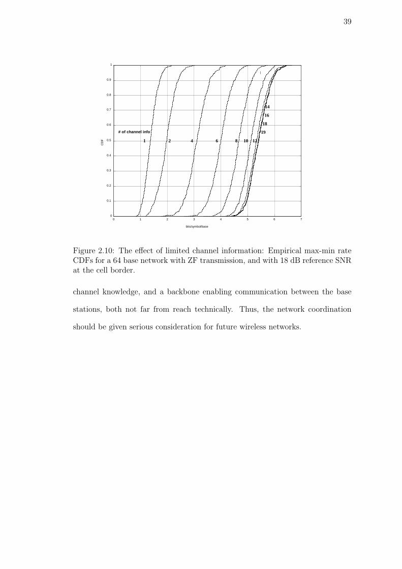
2.10. The effect of limited channel information: Empirical max-min rate
CDFs for a 64 base network with ZF transmission, and with 18 dB
reference SNR at the cell border. . . . . . . . . . . . . . . . . . . 39
3.1. The heuristic user-ordering algorithm for multiple antenna networks. 48
3.2. Empirical max-min rate CDFs: Multiple antenna power control
results for a 64 base network. . . . . . . . . . . . . . . . . . . . . 51
3.3. Empirical max-min rate CDFs: Multiple antenna zero-forcing re-
sults for a 64 base network. . . . . . . . . . . . . . . . . . . . . . 51
3.4. Empirical max-min rate CDFs: Multiple antenna zero-forcing dirty
paper coding results for a 64 base network. . . . . . . . . . . . . . 52
3.5. Spectral efficiency v.s. # of antennas. . . . . . . . . . . . . . . . . 53
3.6. Summary of the multiple antenna results. The results for a conven-
tional network with each base antenna transmitting at the maxi-
mum power limit is also presented. . . . . . . . . . . . . . . . . . 53
4.1. 3 transmit antennas and 2 mobiles with orthogonal channels. . . . 64
4.2. Optimum zero-forcing beamforming vs. Moore-Penrose pseudo-
inverse zero-forcing: 2 users with single antenna receivers. . . . . . 70
4.3. Optimum zero-forcing beamforming vs. Moore-Penrose pseudo-
inverse zero-forcing: 4 users with single antenna receivers. . . . . . 71
4.4. Optimum zero-forcing beamforming vs. Moore-Penrose pseudo-
inverse zero-forcing: 8 users with single antenna receivers. . . . . . 72
5.1. A sample network topology. . . . . . . . . . . . . . . . . . . . . . 77
5.2. The outline of the two steps hierarchical solution. . . . . . . . . . 87
5.3. Simulation setup, 19 cells cellular network (2 rings around the
source node). . . . . . . . . . . . . . . . . . . . . . . . . . . . . . 93
ix

5.4. Results for 19 cells cellular network (2 rings around the source
node). Multi-hop throughput is based on the link-based capacity
assignment method. . . . . . . . . . . . . . . . . . . . . . . . . . . 94
5.5. Simulation setup, 37 cells cellular network (3 rings around the
source node). . . . . . . . . . . . . . . . . . . . . . . . . . . . . . 95
5.6. Results for 37 cells cellular network (3 rings around the source
node). Multi-hop throughput is based on the link-based capacity
assignment method. . . . . . . . . . . . . . . . . . . . . . . . . . . 96
5.7. Simulation setup, 37 cells cellular network with 2 source nodes. . . 97
5.8. Results for 37 cells cellular network with 2 source nodes. Multi-hop
throughput is based on the link-based capacity assignment method. 98
5.9. Simulation setup, 37 cells cellular network with 3 source nodes. . . 99
5.10. Results for 37 cells cellular network with 3 source nodes. Multi-hop
throughput is based on the link-based capacity assignment method. 100
5.11. Single carrier vs OFDMA. 19 cells cellular network (2 rings around
the source node). . . . . . . . . . . . . . . . . . . . . . . . . . . . 101
5.12. Spatial water-filling, random link assignments, link-based water-
filling. 19 cells cellular network (2 rings around the source node).
Results are presented for 0.5µs and 32µs delay spreads. . . . . . . 101
x

1
Chapter 1
Introduction
As the demand for wireless applications continues to grow, future wireless systems
are engineered to provide high-speed broadband services with quality of service
(QoS) support for a wide range of applications, including voice and multimedia
data. The design of such advanced network architectures is a challenging task.
First of all, radio resources such as power and bandwidth are often scarce. There-
fore, efficient resource allocation and network optimization are vital. Secondly,
the wireless channel has its unique impairments such as fading and multi-path.
Also, the mobiles sharing a common communication medium interfere with each
other. The future wireless system designs are expected to address all these chal-
lenges, and networks with high spectral efficiency is a major design goal.
Traditionally, channel fading and multi-path are thought of as impairments
that have to be dealt with. A breakthrough technique which dramatically changed
this point of view is the use of multiple antennas at the transmitters and/or re-
ceivers [1–3]. The advantage of multiple input-multiple output (MIMO) antenna
arrangements is that, when the wireless channel provides a rich scattering envi-
ronment, multiple independent signal paths can be obtained between two com-
municating units employing multiple antennas. In this case, the link capacity
can scale linearly with the number of antennas deployed, even without increasing
transmit power or bandwidth.

2
0 10 20 30 40 50 600
50
100
150
24dB
18 dB
12dB
6 dB
0 dB
# of transmit/receive antennas
Cap
acity
in b
its/s
ymbo
l
Figure 1.1: MIMO capacity gains in a point-to-point link.
The tremendous capacity improvement predicted by the multiple antennas
attracted a huge attention within the research community [4–23]. In addition to
the experimental verification and the measurement of these gains [5], multiple
antennas have been successfully employed in a number of commercial products,
especially in short-range wireless local area networks (WLANs); see for example
[24]. However, the deployment of multiple antennas in cellular networks has not
been successful so far. One important reason is that cellular networks suffer from
inter-cell interference. Therefore, the link qualities in cellular networks can be
relatively poor compared to short-range radio links. On the other hand, the
multiple antenna gain, in terms of marginal increase in rate when an additional
antenna is deployed, is especially large when the signal-to-noise ratio (SNR) is
high [6]. This fact can be observed in Figure 1.1 illustrating capacity gains in
3
a point-to-point link. The figure shows that the slope of the capacity vs. the
number of antennas curve is small when the received SNR is low. For example,
at 0 dB SNR, adding one more antenna to both the transmitter and the receiver
contributes an additional ≈ 0.65 bits/symbol to the spectral efficiency, while the
capacity improves by about 6.5 bits/symbol when the SNR is 24 dB. In realistic
cellular environments, the received SNR is typically around 18 dB when the mobile
is close to the cell border. On the other hand, when the inter-cell interference is
present, the SINR (signal-to-noise-plus-interference ratio) may drop to 0 dB. In
this case, the improvement due to multiple antennas would be very limited if the
interference is not successfully mitigated, as in the conventional cellular networks.
In this dissertation, we propose novel techniques that enable efficient use of
multiple antennas in cellular networks. In particular, we study network coordina-
tion as a means to provide spectrally efficient communications in cellular downlink
systems. When the network coordination is employed, all base antennas act to-
gether as a single network antenna array, and each mobile may receive useful
signals from several nearby base stations. Furthermore, the antenna outputs are
chosen in ways to minimize the out-of-cell interference, and hence to increase
the downlink system capacity. When the out-of-cell interference is mitigated, the
links can operate in the high SNR regime. This enables the cellular network to
enjoy the great spectral efficiency improvement associated with using multiple
antennas.

4
1.1 Related Work
The pioneering multiple antenna studies are due to [1–3]. The initial multiple an-
tenna research mainly focused on point-to-point links. In particular, [1,2] showed
that the link capacity scales linearly with the minimum of the number of trans-
mit and receive antennas. This result requires that the wireless channel provides
enough scattering so that each antenna pair would experience an independent
channel fading and the matrix channel between the transmitter and the receiver
becomes full-rank. Also, the channel information must be available at the re-
ceiver. The availability of the channel information at the transmitter enables
optimal water-filling power allocation on the eigen-modes of the channel [2]. A
number of efficient coding/modulation techniques that help to realize the pre-
dicted capacity gains can be found in [6–10].
Multi-user multiple antenna problems are studied in the context of, first,
multi-access channels [11–15], and then broadcast channels [16–21]. The capac-
ity region of the multiple antenna multi-access channel follows easily from the
capacity region of its scalar counterpart [25]. Basically, successive interference
cancelation extends to the multiple antenna system [11]. In this case, each corner
point on the boundary of the capacity region corresponds to a particular user
order, and each user selects its optimal single-user transmit covariance assuming
the existence of interference due to un-canceled interferers in the user order. The
multiple antenna broadcast channel problem is much more difficult because it is
a nondegraded broadcast channel [25]. Recently, there has been progress towards
characterizing its capacity region. Namely, the dirty paper coding [26,27], which
is a technique to cancel the interference causally known to the transmitter with-
out any transmit power penalty, achieves the boundary of the broadcast capacity

5
region [19, 20]. The multi-access and the broadcast capacity regions are related
through a duality relationship [18]. The usefulness of this relationship is that rel-
atively simple multi-access problem can be solved to find optimum transmission
policies achieving a particular point on the dual broadcast capacity region. Note
that a sum-power constraint is assumed in the above broadcast channel problems.
Moreover, the above results are derived for single-cell systems.
While multiple antennas have been studied extensively in the context of point-
to-point links and single-cell systems, the effectiveness of multiple antennas in
multi-cell systems is not well-understood. In fact, some of the above results apply
to multi-cell systems. For example, an uplink multi-cell system with base station
cooperation is essentially equivalent to a single cell system with an increased
receive antenna count. However, the downlink multi-cell model is fundamentally
different from the single cell model. This is mainly due to the fact that each
base station/antenna has its own power constraint in a multi-cell system. In this
case, the results and the tools, such as the uplink-downlink duality developed for
broadcast channels with sum-power constraints, can not be used easily for the
multi-cell downlink model. Therefore, new tools and approaches are necessary to
analyze the multiple antenna multi-cell downlink networks.
In this thesis, the objective is to contribute to the understanding of the mul-
tiple antennas in cellular networks. To achieve this goal, we consider coordinated
cellular networks where the base stations can communicate and cooperate via a
high-speed backbone. We study the performance limits of such networks with
and without multiple antennas. We investigate the impact of such cooperation
on the effectiveness of multiple antennas. To the best of our knowledge, this
thesis is the first study proposing network coordination as a means to improve
6
the performance of multiple antennas in cellular networks. For earlier studies on
base station cooperation, see [28] for an uplink multi-cell system. We should note
that it is hard to derive analytical expressions in multi-cell formulations since the
results depend heavily on the network topology. Thus, [28] considers a limited
circular network topology to investigate the effect of joint-decoding on the uplink
multi-cell network. For downlink networks, [29] studied the base station coop-
eration. Considering single antenna base stations and mobiles, and assuming a
sum-power constraint relaxation, simple analytical expressions are derived for the
capacity of such networks.
1.2 Overview of Dissertation
The thesis study starts with the analysis of the downlink cellular networks with
single antenna base stations and mobiles. In Chapter 2, we examine coordinated
networks in which a high-speed backbone enables all network antennas to operate
as a single network-wide antenna array. We compare the max-min rate perfor-
mance of practical coordination techniques to that of a conventional network with
power control. We show that the coordinated base antenna transmissions provide
large capacity improvements over the conventional cellular networks.
In Chapter 2, we also study the theoretical performance limits of coordination.
Our system can be modeled as a non-degraded Gaussian broadcast channel for
which the optimal scheme achieving the boundary of the capacity region involves
the dirty paper coding [19, 27]. However, characterizing the max-min rate point
on the capacity region is nontrivial as the dirty paper rate functions are in general
non-concave in transmit covariances [18]. In this case, the optimal policy may

7
involve time-sharing, and one may need to specify time-sharing combinations as
well as a user ordering for the dirty paper encoding. This becomes computa-
tionally infeasible for large systems as one needs to search over all possible user
combinations and encoding orders. Our approach is to develop tight upper bounds
on the max-min rate. We show that the rate achievable by a particular form of
zero-forcing dirty paper coding scheme combined with a heuristic user ordering
is very close to the sharpest upper bound obtained. The established bounds not
only help to avoid a huge computational burden, but also they give insights into
the ultimate performance of the system.
Also in Chapter 2, we discuss the impact of sectorization on the downlink
performance. We compare sectorization with coordination, and then consider a
coordinated network architecture with sectorization. While the sectorization by
itself helps to reduce inter-cell interference, employing network coordination with
sectorization gives substantial additional improvements in system capacity. In
this chapter, we also discuss some implementation issues such as availability of
channel information. In particular, we evaluate the system performance when
only a partial channel information is available at the transmitters.
In Chapter 3, we study the impact of network coordination on multiple an-
tenna systems. We show that the coordinated transmissions are especially effec-
tive when the base stations and the mobiles are equipped with multiple antennas.
Note that deploying multiple antennas in a cellular network is a challenging task
due to its complexity of implementation and the cost of infrastructure upgrades
in the current cellular architecture. In order to justify the use of multiple anten-
nas in a cellular network, the predicted multiple antenna gains must be realized

8
in practice. In this chapter, we show how to design a coordinated network em-
ploying multiple antennas. Our results indicate that the interference mitigation
capability of network coordination enables the cellular network to enjoy the great
spectral efficiency improvement associated with using multiple antennas.
In Chapters 2 and 3, we study coordination techniques that require simple,
practical linear beamforming techniques. While these beamforming methods pro-
vide significant capacity improvements over the conventional cellular networks,
they are not claimed to be the optimal linear coordination techniques. The objec-
tive in Chapter 4 is to find the optimum beamforming vectors. More specifically,
in all problem formulations in the thesis, we consider per-antenna power con-
straints for which well-known beamforming techniques such as the pseudo-inverse
zero-forcing is suboptimal. We show that finding the optimum beamforming vec-
tors requires solving a convex optimization problem. We will see that optimizing
the antenna outputs based on the per-antenna constraints may improve the rate
considerably when the number of transmit antennas is much larger the number
of receive antennas. The reason is that more transmit antennas will give more
degrees of freedom to optimize the antenna outputs. When the number of trans-
mit and receive antennas are close to each other, there are not much room left to
exploit in the signal space.
The network coordination techniques assume the existence of a high-speed
backhaul enabling communications between the base stations. In Chapter 5, we
study the design of such a backhaul in a cellular network. In particular, we con-
sider a mesh backhaul network consisting of fixed base stations (mesh routers)
connected by wireless links. Some of the mesh routers are assumed to have con-
nections to the wired network, and therefore can function as gateways. The

9
network has multi-hop capability where the traffic entering the mesh backhaul
through the gateway routers can be carried over multiple wireless links towards
the destination mesh routers. The objective in this chapter is to study the perfor-
mance limits of such networks. Assuming the use of an OFDMA air-interface for
the mesh backhaul network, we formulate a cross-layer optimization problem that
involves power control, channel allocation, link scheduling and routing. We show
that when the radio resources are optimized carefully, OFDM transmissions may
provide tone-diversity advantage in the form of efficient bandwidth utilization by
choosing better channels for transmissions and scheduling, or in the form of im-
proved routing performance by providing more path options to route the traffic.
Our numerical results indicate that OFDMA-based mesh architecture provides
an efficient backhaul solution in cellular networks.

10
Chapter 2
Network Coordination for Single Antenna Base
Stations and Mobiles
In conventional cellular systems, each base station transmits signals intended for
users within its cell coverage. Depending on the users’ channel conditions, in-
terference caused by the neighboring cell transmissions can sharply degrade the
received signal quality. Thus, the downlink capacity of cellular wireless networks
is limited by inter-cell interference. Fortunately, since the base stations can be
connected via a high-speed backbone, there is an opportunity to coordinate the
base antenna transmissions so as to minimize the inter-cell interference, and hence
to increase the downlink system capacity. In this chapter, we study various as-
pects of network coordination in cellular downlink systems.
Figure 2.1 shows the basic idea of the network coordination. On the top figure,
the base antenna transmissions are not coordinated, and therefore neighboring
base transmissions are received as inter-cell interference (each color represents a
signal useful for a given mobile). The objective of network coordination is to
enable cooperation between the base stations so that useful signals, as opposed
to the interference, can be received from the neighboring base antennas. In the
following, we will describe the transmission techniques achieving this objective.

11
signal (solid, bold)
interference (dotted)
signal (solid, bold)
useful signal (dotted)
Figure 2.1: Conventional Cellular Networks (top) vs. Coordinated Networks(bottom).
2.1 System Model
In general, the system model for a downlink network with M single antenna base
stations and N single antenna mobiles is given by
Y = Hx + n (2.1)
where H = [hij]N×M denotes the channel matrix with hij being the complex
channel gain between mobile i and base station j, x = [x1, x2, . . . , xM ]T denotes
the complex antenna outputs, and n = [n1, n2, . . . , nN ]T denotes an additive
white noise vector with covariance σ2I. When coordination is employed, all M
base stations can act together, and each mobile may receive useful signals from
all base stations. Denoting the vector of data symbols by d = [d1, d2, . . . , dN ]T
where di is the ith mobile’s complex data symbol, a linear spatial pre-filter matrix
A ∈ CM×N is used to map the data symbols to the antenna outputs, i.e. x = Ad.

12
Thus, in the case of coordination, the antenna output at the jth base station is a
linear combination of N data symbols, i.e., xj =∑N
i=1 Ajidi. For the conventional
cellular transmissions, each base station simply transmits the data symbol for the
mobile in its own cell coverage, and the linear pre-filter matrix is not necessary.
In our analysis, we assume that each base is loaded at most with one user, i.e.,
N ≤ M . For example, the system model (2.1) may correspond to the set of
mobiles using a particular orthogonal dimension, i.e., a time slot for TDMA, a tone
for OFDM, an orthogonal spreading code for CDMA etc., in each base station,
and some of the mobiles may be in outage due to their undesirable channel and
interference conditions.
In the following sections, we will present different transmission techniques,
and explain the methodology for their performance evaluations. The metric for
comparison will be the max-min rate achievable subject to per-base power con-
straints. The max-min rate objective is motivated by the fairness concern, i.e.,
the need to guarantee a quality of service (QoS) for a large number of users spread
over many cells.
2.2 Conventional Cellular Network
The baseline for comparison with the coordinated networks is the conventional
cellular systems without network coordination. In this case, each base station
transmits signals intended for the user within its cell coverage, and neighboring
base transmissions cause inter-cell interference. Given the model (2.1), the an-
tenna output at the ith base antenna is the data symbol for its associated mobile,

13
i.e., xi = di. Denoting the power of the ith data symbol by pi, the signal-to-
interference-plus-noise ratio (SINR) for mobile i is given by
ρi =pi|hii|2∑
j 6=i pj|hij|2 + σ2. (2.2)
and the corresponding Shannon rate is given by log2(1 + ρi) bits/symbol/Hz.
The following optimization problem formulates the max-min rate problem for an
uncoordinated network subject to per-base power constraints:
max r (2.3)
s.t. log2
(1 +
pi|hii|2∑j 6=i pj|hij|2 + σ2
)≥ r (2.3a)
0 ≤ pi ≤ pmax, i = 1, . . . , N (2.3b)
r ∈ <+, pi ∈ <+ (2.3c)
where pmax is the maximum transmit power of a base station antenna, and r
can be interpreted as the minimum rate to be maximized, i.e., r = mini log2(1 +
ρi). The max-min rate can be found in an iterative fashion by solving a series
of linear feasibility problems. One can initially start with a small target rate
r, and can solve a simple linear system of equations to find if there exists a
feasible power allocations (either as a centralized LP or using distributed power
control algorithms). The target rate is improved further as long as the power
constraints are satisfied. We note that channel phase knowledge is not needed for
uncoordinated transmissions.
14
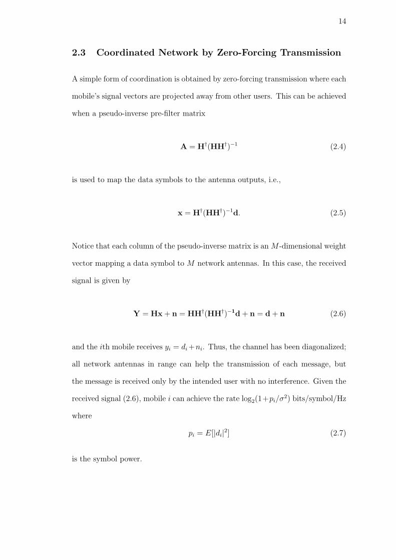
2.3 Coordinated Network by Zero-Forcing Transmission
A simple form of coordination is obtained by zero-forcing transmission where each
mobile’s signal vectors are projected away from other users. This can be achieved
when a pseudo-inverse pre-filter matrix
A = H†(HH†)−1 (2.4)
is used to map the data symbols to the antenna outputs, i.e.,
x = H†(HH†)−1d. (2.5)
Notice that each column of the pseudo-inverse matrix is an M -dimensional weight
vector mapping a data symbol to M network antennas. In this case, the received
signal is given by
Y = Hx + n = HH†(HH†)−1d + n = d + n (2.6)
and the ith mobile receives yi = di +ni. Thus, the channel has been diagonalized;
all network antennas in range can help the transmission of each message, but
the message is received only by the intended user with no interference. Given the
received signal (2.6), mobile i can achieve the rate log2(1+pi/σ2) bits/symbol/Hz
where
pi = E[|di|2] (2.7)
is the symbol power.

15
To formulate the max-min rate optimization problem, one has to specify per-
base power constraints. Notice that each base antenna is subject to an average
power constraint given by E[|xm|2] ≤ pmax, m = 1, . . . , M . These constraints can
be transformed into a set of linear constraints in terms of the power of the data
symbols pi, i = 1, . . . , N . Note that base antenna powers are on the diagonals of
the following transmit covariance matrix
E[xx†] = AE[dd†]A† = A
p1
. . .
pN
A†, (2.8)
where x = Ad, and assuming independent data symbols, the constraints on the
diagonals can be expressed in matrix form as
|A11|2 . . . |A1N |2...
...
|AM1|2 . . . |AMN |2
p1
...
...
pN
≤ pmax1 (2.9)
where 1 = [1, 1, . . . , 1]T is an M-dimensional column vector of 1s. The problem
of maximizing the minimum rate subject to per-base power constraints can be
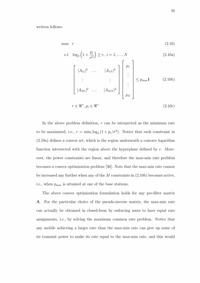
16
written follows:
max r (2.10)
s.t. log2
(1 +
pi
σ2
)≥ r, i = 1, . . . , N (2.10a)
|A11|2 . . . |A1N |2...
...
|AM1|2 . . . |AMN |2
p1
...
...
pN
≤ pmax1 (2.10b)
r ∈ <+, pi ∈ <+ (2.10c)
In the above problem definition, r can be interpreted as the minimum rate
to be maximized, i.e., r = mini log2 (1 + pi/σ2). Notice that each constraint in
(2.10a) defines a convex set, which is the region underneath a concave logarithm
function intersected with the region above the hyperplane defined by r. More-
over, the power constraints are linear, and therefore the max-min rate problem
becomes a convex optimization problem [30]. Note that the max-min rate cannot
be increased any further when any of the M constraints in (2.10b) becomes active,
i.e., when pmax is attained at one of the base stations.
The above convex optimization formulation holds for any pre-filter matrix
A. For the particular choice of the pseudo-inverse matrix, the max-min rate
can actually be obtained in closed-form by enforcing users to have equal rate
assignments, i.e., by solving the maximum common rate problem. Notice that
any mobile achieving a larger rate than the max-min rate can give up some of
its transmit power to make its rate equal to the max-min rate, and this would

17
actually help the power constraints. Under the equal rate constraint, each user’s
received power would be the same p. In this case, the covariance matrix simply
becomes E[xx†] = pAA†. Similarly, the base antenna power constraints on the
diagonals of the covariance matrix can be written as
p[AA†](j,j) = p
N∑i=1
|Aji|2 ≤ pmax, j = 1, . . . , M, (2.11)
where [.](j,j) denotes the jth diagonal element of the matrix. Maximizing the
common rate is equivalent to maximizing the common received power p, which
occurs at p∗ = pmax/ maxj
∑Ni=1 |Aji|2. It follows that the maximum common rate
is given by r∗ = log2(1 + p∗/σ2), which is also equivalent to the max-min rate.
We mention that an MMSE pre-filter is also possible [31, 32], which should
have a performance beyond that of the zero-forcing scheme. However, as we will
see in the numerical examples section, the typical cellular network setup that we
are interested in will have a relatively high SNR, and therefore we expect the
performance improvement due to MMSE pre-filter to be small. Also, complete
channel knowledge (including phase and magnitude) is needed for the zero-forcing
technique, as well as for the zero-forcing dirty paper coding technique of the next
section.
2.4 Coordinated Network by Zero-Forcing Dirty Paper
Coding
Zero-forcing comes with a penalty in the sense that a mobile’s transmissions are
constrained to a smaller subspace after projecting away from the other mobiles’

18
channels. An improved form of coordination is obtained when a limited form of
zero-forcing is combined with dirty paper coding [20,29]. Dirty paper coding can
be employed when the interference is known causally at the transmitter, which
is possible for downlink transmissions. First, mobiles are indexed according to
some order π = [π(1), π(2), . . . , π(N)]. By dirty paper encoding, a mobile can be
made invisible interference-wise to other mobiles with higher indices in the user
ordering [27]. When dirty paper coding is combined with a limited form of zero
forcing, the visible interference is nulled out due to the zero forcing.
The combined zero-forcing dirty paper coding scheme assumes a linear pre-
filter matrix A obtained through LQ decomposition of the channel matrix H, and
is given by A = Q† where H = LQ, L ∈ CN×N is lower triangular, and Q ∈ CN×M
is a unitary matrix with QQ† = I [20,29]. We should note that while this scheme
is shown to be sum-rate optimal at high SNR regime subject to a sum power
constraint, the same scheme is not claimed to be optimal for the max-min rate
problem subject to per-base power constraints. The corresponding system model
(2.1) is given by
Y = Hx + n = HAd + n = LQQ†d + n = Ld + n. (2.12)
Therefore the ith user receives the signal
yi = Liidi +∑j<i
Lijdj + ni. (2.13)
The particular choice of spatial filter matrix A = Q† nulls the interference
from users with indices j > i, and the remaining part of the interference due to

19
users with indices j < i (causally known to the transmitter) is taken care of by
the dirty paper coding [27]. In this case, the ith user experiences a single user
channel, and can achieve the following rate
ri = log2
(1 +
|Lii|2pi
σ2
)(2.14)
where pi = E[|di|2]. Each base station antenna is subject to an average power
constraint given by
E[|xm|2] ≤ Pmax, m = 1, . . . ,M. (2.15)
Next, the base antenna power constraints are transformed into a set of linear
constraints in terms of power of the data symbols pi, i = 1, . . . , N . Note that base
antenna powers are on the diagonals of the following transmit covariance matrix
E[xx†] = Q†E[dd†]Q = Q†
p1
. . .
pN
Q. (2.16)
The constraints on the diagonals can be expressed in matrix form as
|Q11|2 . . . |QN1|2...
...
|Q1M |2 . . . |QNM |2
p1
...
...
pN
≤ pmax1 (2.17)
where 1 = [1, 1, . . . , 1]T is an N-dimensional column vector of 1s. The problem
20
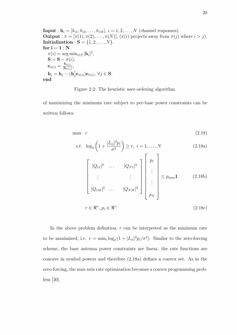
Input : hi = [hi1, hi2, . . . , hiM ], i = 1, 2, . . . , N (channel responses).Output : π = [π(1), π(2), . . . , π(N)], (π(i) projects away from π(j) where i > j).Initialization : S = {1, 2, . . . , N}.for i = 1 : N
π(i) = arg mini∈S |hi|2,S = S− π(i),
eπ(i) =hπ(i)
|hπ(i)| ,
hj = hj − (h†jeπ(i))eπ(i), ∀j ∈ S.end
Figure 2.2: The heuristic user-ordering algorithm.
of maximizing the minimum rate subject to per-base power constraints can be
written follows:
max r (2.18)
s.t. log2
(1 +
|Lii|2pi
σ2
)≥ r, i = 1, . . . , N (2.18a)
|Q11|2 . . . |QN1|2...
...
|Q1M |2 . . . |QNM |2
p1
...
...
pN
≤ pmax1 (2.18b)
r ∈ <+, pi ∈ <+ (2.18c)
In the above problem definition, r can be interpreted as the minimum rate
to be maximized, i.e. r = mini log2 (1 + |Lii|2pi/σ2). Similar to the zero-forcing
scheme, the base antenna power constraints are linear, the rate functions are
concave in symbol powers and therefore (2.18a) defines a convex set. As in the
zero-forcing, the max-min rate optimization becomes a convex programming prob-
lem [30].

21
The above combined zero-forcing dirty paper coding scheme assumes a user
ordering. Notice that when a particular user i’s transmission becomes invisi-
ble to some others due to dirty paper encoding, those users who do not receive
interference from user i do not have to project away from this particular user.
Moreover, dirty paper encoding does not induce any power penalty [27], and
therefore comes for free (except the complexity of its practical implementation).
On the other hand, zero-forcing incurs a penalty in the sense that a user pro-
jecting its signals away from others would give up some part of its signal space.
Since the objective is fairness, we propose a heuristic user ordering based on the
idea that the price should be paid by the users with good channels. In this case,
a user with a good channel “owes a favor” to users with relatively bad channels,
and therefore projects away form those disadvantageous users. In turn, the users
with bad channels “pay the favor back” by being invisible via the dirty paper
encoding. The heuristic user ordering algorithm is shown in Figure 2.2. We will
see in the numerical examples section that the algorithm performs quite well in
our cellular network setup.
2.5 Performance Limits of Network Coordination
Thus far, we have considered coordination techniques that involve practical linear
filtering operations, and thus are analytically tractable. In this section, our ob-
jective is to study the ultimate performance limits of network coordination, and
see how far the techniques of the previous sections are from the ultimate limits.
The system model described in (2.1) is an example of a non-degraded Gaussian
broadcast channel with M geographically separated but perfectly cooperating

22
transmitters, and N non-cooperating receivers. Finding the capacity region for
such channels has been a major research challenge for a long time. Recently,
it has been shown that subject to sum power constraint E[|x|2] ≤ pmax, the
optimal scheme achieving the boundary of the capacity region involves dirty paper
coding [19,20], where the transmitter encodes N data symbols in an order given by
[π(1), . . . , π(N)] such that a user with index π(i) does not suffer any interference
from users with lower indices, i.e., π(j) with j < i. Moreover, the optimal policy
may involve time-sharing, as the dirty paper rate functions are in general non-
concave in transmit covariances [18].
Notice that, unique to our multiple base coordinated network model, we have
a set of constraints and assumptions that adds a new dimension to the classical
broadcast channel problems. First, instead of a sum-power constraint, we are
concerned with per-base (or per-antenna) power constraints as the transmit power
cannot be transferred from one base station to the other. Second, we have a
large number of users spread over many cells, and therefore we would like to
guarantee a quality of service (QoS) for each user. Hence, our objective is to
maximize the minimum rate in the network, instead of a more common sum-rate
objective. The classical approach to solve this problem would be to characterize
the capacity region with per-base power constraints, and then determine the
policy maximizing the minimum of all rates. The difficulty is that even with
the duality results [18], it is computationally hard to derive policies, i.e., an
encoding order and corresponding transmit covariances etc., achieving a specific
point (max-min point in our case) on the broadcast capacity region. Moreover,
when the optimal policy involves time-sharing, one may need to specify time-
sharing combinations as well. This becomes computationally infeasible for large

23
systems as one needs to search over all possible user combinations and encoding
orders. Therefore, our approach is to develop tight upper bounds on the max-min
rate. These bounds not only help to avoid a huge computational burden, but also
they give insights into the ultimate performance of the system.
2.5.1 Upper Bounds on the Max-Min Rate of a Coordi-
nated Network
In this section, we derive upper bounds on the max-min rate achievable in a co-
ordinated network. From the first upper bound to the last, each upper bound
improves the tightness of the previous upper bounds at the expense of an in-
creased computational complexity. The common context of all the derivations
is a configuration that has no user suffering interference. Although, at the first
sight this may seem to be too drastic a departure, we will establish its usefulness.
Recall that the optimum transmission scheme involves some form of dirty paper
coding, with which users causing significant interference can be made invisible to
others. Because of the no-interference assumption, each user enjoys a single user
channel with M transmit antennas. However, multiple users are coupled through
power sharing, i.e., each of them competes for a portion of the total available
power.
The interference-free assumption will enable us to work with concave rate
functions in user covariances so that the standard convex optimization techniques
can be easily employed. On the other hand, for any transmission policy, the set of
rates calculated based on no interference will be an upper bound on the actual user
rates. Importantly, the bounds are valid even when the optimal policy involves

24
time sharing. The reason is that, without interference, we are left with single
user channels in which it is better not to do time sharing due to concavity of the
logarithm function. In other words, time sharing rates, which are already upper
bounded by ignoring the interference, will be further bounded when we restrict our
attention to simpler transmission policies. Also, when users do not interfere with
each other, the issue of dirty paper encoding order becomes irrelevant. Therefore,
the bounds are valid for all encoding orders when the optimal transmission policy
involves the dirty paper coding. In short, by being reasonably optimistic, we
greatly simplify a complex problem as we do not have to deal with all permutations
of dirty paper encoding order, or time-sharing combinations.
Single-User Bound
Our first upper bound is based on a single-user argument that the network does
its best for one of the users by granting him exclusive use of all network re-
sources. In other words, the network operator lets all M base station antennas
serve the user at full power, and produce a coherently reinforced signal at the
user’s antenna. Let us consider user i, and assume that the antenna at the
mth base transmits a voltage vim =√
pimejφim to this user, where pim is the
transmit power and φim is the phase. In this case, the transmit voltage vector
is given by vi = [vi1, vi2, . . . , viM ]T . Given the ith user’s complex vector chan-
nel hi = [hi1, hi2, . . . , hiM ]T , the maximum received signal power is obtained by
having phase matched transmit voltages, and coherent voltage addition at the
receiver side. In this case, the ith user achieves the single user rate given by
ri = log2
(1 +
(√pi1|hi1|+ · · ·+√
piM |hiM |)2
σ2
). (2.19)

25
Given that all base antennas transmit at full power, i.e. pim = pmax for
m = 1, . . . , M , (2.19) can be written as ri = log2(1 + pmax‖hi‖21/σ
2), where ‖hi‖1
denotes L1 norm of the vector channel hi. The first upper bound is based on the
fact that max-min rate of N users cannot exceed the single user Shannon rate of
any user (2.19). Therefore, denoting the max-min rate by r, it follows that
r ≤ mini∈{1,...,N}
log2
(1 +
pmax‖hi‖21
σ2
)(2.20)
Multi-User Bound with Sum-Power Constraint
We can improve the previous upper bound by considering presence of multiple
users in the system. Similar to the first bound, we assume that users do not
suffer any interference, but they are coupled through power sharing. Given the
ith user’s transmit voltage vector vi = [vi1, vi2, . . . , viM ]T , and the channel hi =
[hi1, hi2, . . . , hiM ]T , the received signal power is |vi · hi|2, which is by coherent
voltage addition. In this case, each user achieves the following rate
ri = log2
(1 +
|vi · hi|2Ii + σ2
)i = 1, . . . , N (2.21)
where Ii denotes the total interference power user i would actually suffer. An
upper bound on the max-min rate r can be written as
r ≤ ri = log2
(1 +
|vi · hi|2Ii + σ2
)(a)
≤ log2
(1 +
|vi · hi|2σ2
)
(b)
≤ log2
(1 +
‖vi‖2‖hi‖2
σ2
), (2.22)

26
where (a) is obtained by ignoring the interference term Ii, and (b) is due to
the Cauchy-Schwartz inequality. In the inequality (2.22), the magnitude squared
voltage term ‖vi‖2 represents the total power allocated to the ith user across all
base stations; we denote it by Pi = ‖vi‖2. It follows from (b) that
(2r − 1)σ2
|hi‖2≤ Pi. (2.23)
The sum-power of all users must be smaller than the total available power in
the network implyingN∑
i=1
Pi ≤ Mpmax. (2.24)
This is a relaxation to per-base power constraints, which will be analyzed in
the following subsection, and will lead to a better upper bound. It follows that
(2r − 1)N∑
i=1
σ2
‖hi‖2≤
N∑i=1
Pi ≤ Mpmax (2.25)
The second upper bound follows easily from (2.25):
r ≤ log2
(1 +
Mpmax∑Ni=1
σ2
‖hi‖2
). (2.26)
Multi-User Bound with Per-Base Power Constraint
A tighter upper bound is obtained by considering per-base power constraints, in-
stead of the previous section’s constraint relaxation in the form of a sum-power
constraint. Note in the previous section that Pi represents the sum of contribu-
tions of each antenna power for user i, i.e., Pi =∑M
m=1 pim. Here, we will choose,

27
for each user, transmit powers at each base so as to satisfy per base power con-
straints given byN∑
i=1
pim ≤ pmax, m = 1, . . . , M (2.27)
Consider the following optimization problem:
max r′
(2.28)
s.t. (2r′− 1)
σ2
‖hi‖2−
M∑m=1
pim ≤ 0, i = 1, . . . , N (2.28a)
N∑i=1
pim ≤ pmax, m = 1, . . . , M (2.28b)
r′ ∈ <+, pim ∈ <+ (2.28c)
where the constraint (2.28a) expresses the bound (2.22b) using the definition of
Pi in this section. The solution to the optimization problem, say r∗, is an upper
bound on the max-min rate, i.e., r ≤ r∗. The argument is that, for r′
= r,
the optimum power, and phase allocations maximizing the minimum rate, i.e.,
achieving r, would satisfy (2.22b), and therefore (2.28a) as well. Moreover, the
optimum power allocations are feasible, and therefore the constraint (2.28b) is also
satisfied. Thus, we would at least obtain r by solving the optimization problem
(2.28), and possibly overshoot r due to the constraint relaxation (2.28a). The
optimization problem can easily be solved as a convex program, or as a linear
program (LP) by defining an auxiliary variable t = 2r′ − 1, and maximizing t
subject to the constraints (2.28a)-(2.28c). Since t is an increasing function of r′,
maximizing t would maximize r′
as well. If the solution occurs at t∗, then r∗
simply follows as r∗ = log2 (1 + t∗).
28
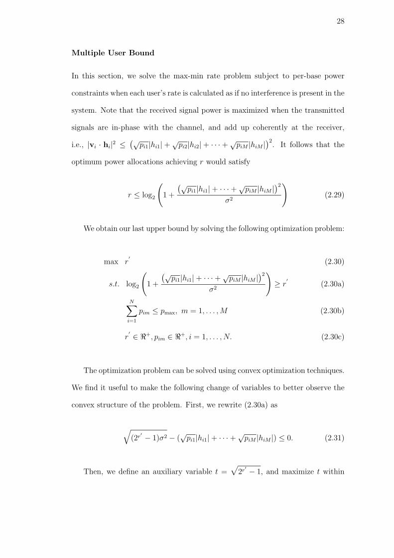
Multiple User Bound
In this section, we solve the max-min rate problem subject to per-base power
constraints when each user’s rate is calculated as if no interference is present in the
system. Note that the received signal power is maximized when the transmitted
signals are in-phase with the channel, and add up coherently at the receiver,
i.e., |vi · hi|2 ≤(√
pi1|hi1|+√pi2|hi2|+ · · ·+√
piM |hiM |)2
. It follows that the
optimum power allocations achieving r would satisfy
r ≤ log2
(1 +
(√pi1|hi1|+ · · ·+√
piM |hiM |)2
σ2
)(2.29)
We obtain our last upper bound by solving the following optimization problem:
max r′
(2.30)
s.t. log2
(1 +
(√pi1|hi1|+ · · ·+√
piM |hiM |)2
σ2
)≥ r
′(2.30a)
N∑i=1
pim ≤ pmax, m = 1, . . . , M (2.30b)
r′ ∈ <+, pim ∈ <+, i = 1, . . . , N. (2.30c)
The optimization problem can be solved using convex optimization techniques.
We find it useful to make the following change of variables to better observe the
convex structure of the problem. First, we rewrite (2.30a) as
√(2r
′ − 1)σ2 − (√
pi1|hi1|+ · · ·+√piM |hiM |) ≤ 0. (2.31)
Then, we define an auxiliary variable t =√
2r′ − 1, and maximize t within

29
the constraints (2.30a)-(2.30c). Since t is an increasing function of r′, maximizing
t would maximize r′as well. Also, we define yim =
√pim, and solve the following
optimization problem:
max t (2.32)
s.t. tσ − (yi1|hi1|+ · · ·+ yiM |hiM |) ≤ 0, (2.32a)
N∑i=1
y2im ≤ pmax, m = 1, . . . , M, (2.32b)
t ∈ <+, yim ∈ <+, i = 1, . . . , N. (2.32c)
The first set of constraints (2.32a) is linear in optimization variables, and
therefore defines a convex region. The second set of constraints (2.32b) defines
an intersection of spheres, which is also convex. Thus, the problem is a convex
optimization problem with linear and non-linear constraints. The solution of such
a convex optimization problem is well-known [30].
2.6 Coordination vs. Sectorization
Another effective method for downlink interference mitigation is the use of sector-
ized antennas at the base station. Sectorization can be interpreted as spatial/fixed
beamforming where directional narrow-beam antennas are used to separate inter-
fering users spatially. On the other hand, the coordination provides user-specific
beamforming, and therefore is more flexible than sectorization. For example, in
our numerical examples, we will present results for a 36 base network with 6 sec-
tors in each cell, and one user per antenna. In this case, when the mobiles are

30
uniformly distributed across the cell area, each sector might have only one user,
and the sectorization can effectively mitigate the intra-cell interference. On the
other hand, if there are more than one user in a sector area, sectorized anten-
nas cannot separate these users while the coordinated antennas can effectively
separate them through zero-forcing or dirty paper coding. We will see in our
numerical examples that while the sectorization by itself helps to reduce inter-cell
interference, employing network coordination with sectorization gives substantial
additional improvements in system capacity.
2.7 Limited Coordination: Partial Channel Information
The coordinated transmission methods require the channel information at the
base station. This could be achieved in practice by using channel estimates on
the uplink in the time division duplexing (TDD) mode, or by a channel feedback
from the mobiles in the frequency division duplexing mode (FDD). However, there
will be channel estimation errors and feedback delays, and therefore availability
of an accurate channel information is a challenge. Here, we consider a limited co-
ordination scenario where only partial information is available about the channel
matrix H. In particular, we assume that, for each mobile antenna, only the chan-
nels of those base antennas with strong enough links can be reliably estimated.
Figure 2.4 shows a sample scenario where only the channel information for the
two base station antennas with the strongest links is available for each mobile
antenna. Here, the partial channel matrix is denoted by Hp. As a case study, we
will consider the zero-forcing coordination where the precoding matrix is chosen
to be A = H†p(HpH
†p)−1 based on the partial channel matrix. In this case, the
31
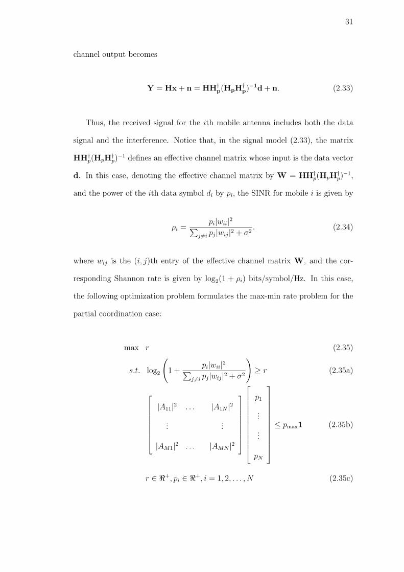
channel output becomes
Y = Hx + n = HH†p(HpH
†p)−1d + n. (2.33)
Thus, the received signal for the ith mobile antenna includes both the data
signal and the interference. Notice that, in the signal model (2.33), the matrix
HH†p(HpH
†p)−1 defines an effective channel matrix whose input is the data vector
d. In this case, denoting the effective channel matrix by W = HH†p(HpH
†p)−1,
and the power of the ith data symbol di by pi, the SINR for mobile i is given by
ρi =pi|wii|2∑
j 6=i pj|wij|2 + σ2. (2.34)
where wij is the (i, j)th entry of the effective channel matrix W, and the cor-
responding Shannon rate is given by log2(1 + ρi) bits/symbol/Hz. In this case,
the following optimization problem formulates the max-min rate problem for the
partial coordination case:
max r (2.35)
s.t. log2
(1 +
pi|wii|2∑j 6=i pj|wij|2 + σ2
)≥ r (2.35a)
|A11|2 . . . |A1N |2...
...
|AM1|2 . . . |AMN |2
p1
...
...
pN
≤ pmax1 (2.35b)
r ∈ <+, pi ∈ <+, i = 1, 2, . . . , N (2.35c)

32
BS
Figure 2.3: Layout for a 64 cells cellular network with a base at the center ofeach hexagon. A cell with two concentric hexagonal rings of surrounding cells ishighlighted.
where the power constraint (2.35b) follows from (2.10b) with the precoding matrix
given by A = H†p(HpH
†p)−1 based on the partial channel.
As in Section 2.2, the max-min rate can be found in an iterative fashion by
solving a series of linear feasibility problems. Notice that the power constraints
(2.35b) are linear. In this case, one can start with a small target rate r, and
can solve a linear system of equations to find if there exists a feasible power
allocations. The target rate is improved further as long as the power constraints
are satisfied.

33
hik
hii
mobile i
×××=
...
...
...
...
Hp ikii hh
base kbase i
Figure 2.4: For each mobile antenna, only the channel information for the twobase station antennas with the strongest links is available.
2.8 Performance Evaluation
In this section, we will present results for a 64 base cellular network. We assume
that each base station is located at the center of an hexagonal cell shown in
Figure 2.3. A flat torus is formed to avoid the boundary effects. From the
base antenna i to the mobile antenna j at a distance of d meters, the channel
propagation characteristic is a triple product, i.e., hij ∝ αijs1/2ij d−ε/2 where in
addition to path-loss with a propagation exponent of ε = 3.8, the channels are
affected by log-normal shadowing sij with 0 mean and 8 dB standard deviation,
and 0 mean unit variance complex Gaussian component αij (Rayleigh piece). We
assume a maximum base power of 10 W, a mean power loss of 134 dB at the

34
1 2 3 4 5 6 7 80
0.1
0.2
0.3
0.4
0.5
0.6
0.7
0.8
0.9
1
bits/symbol/base
CD
F
PCZFZF−DP
Figure 2.5: Empirical max-min rate CDFs for a 64 base network with 18 dBreference SNR at the cell border.
reference distance of 1.6 km from the base (distance from the base station to
any corner of the hexagon), a receiver noise figure of 5 dB, a vertical antenna
gain of 10.3 dBi, a channel bandwidth of 5 MHz, and a receiver temperature of
300oK. Thus, accounting only for path loss and ignoring shadowing and Raleigh
fading, SNR at the reference distance is 18 dB. However, because of inter-cell
interference, the SINR can be much smaller than 18 dB (can even be negative) in
our cellular network setup. In Figure 2.3, two rings around a cell are highlighted to
emphasize that a mobile in the center cell can receive significant signal only from
those colored cells because of the exponential decay in the signal power [35, 36].
In other words, those colored cells may potentially interfere with the mobile in
the center cell, while at the same time they can be coordinated to help overcome
the interference.
Figure 2.5-2.7 show empirical CDFs of the max-min rate for conventional
35
0.5 1 1.5 2 2.5 3 3.5 4 4.5 5 5.50
0.1
0.2
0.3
0.4
0.5
0.6
0.7
0.8
0.9
1
bits/symbol/base
CD
F PCZFZF−DP
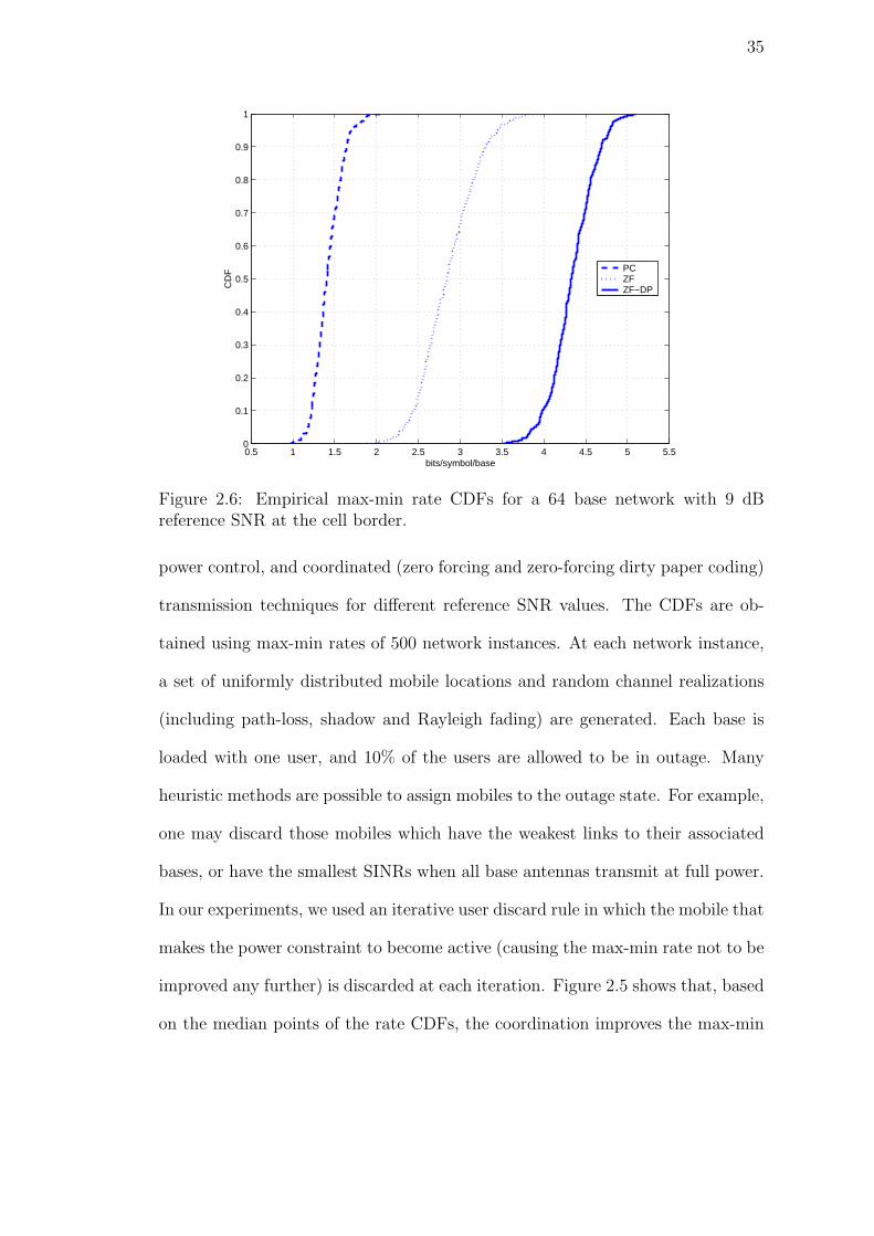
Figure 2.6: Empirical max-min rate CDFs for a 64 base network with 9 dBreference SNR at the cell border.
power control, and coordinated (zero forcing and zero-forcing dirty paper coding)
transmission techniques for different reference SNR values. The CDFs are ob-
tained using max-min rates of 500 network instances. At each network instance,
a set of uniformly distributed mobile locations and random channel realizations
(including path-loss, shadow and Rayleigh fading) are generated. Each base is
loaded with one user, and 10% of the users are allowed to be in outage. Many
heuristic methods are possible to assign mobiles to the outage state. For example,
one may discard those mobiles which have the weakest links to their associated
bases, or have the smallest SINRs when all base antennas transmit at full power.
In our experiments, we used an iterative user discard rule in which the mobile that
makes the power constraint to become active (causing the max-min rate not to be
improved any further) is discarded at each iteration. Figure 2.5 shows that, based
on the median points of the rate CDFs, the coordination improves the max-min

36
0 0.5 1 1.5 2 2.5 30
0.1
0.2
0.3
0.4
0.5
0.6
0.7
0.8
0.9
1
bits/symbol/base
CD
F
PCZFZF−DP
Figure 2.7: Empirical max-min rate CDFs for a 64 base network with 0 dBreference SNR at the cell border.
rate by about a factor-of-3 when the zero-forcing coordination is employed, and by
about a factor-of-5 when the combined zero-forcing dirty paper coding scheme is
used. The reported numbers in Figure 2.5 are based on a typical cellular wireless
channel, and therefore should be interpreted as the potential gains in practical
wireless sytems. To show the dependence of our results to the reference SNR,
we also plotted the rate CDFs for 0 dB and 9 dB reference SNRs in Figure 2.6
and Figure 2.7 respectively. From Figure 2.7, we observe that the zero-forcing,
which performs well at high SNRs, performs far from optimal at very low SNRs.
On the other hand, the combined zero-forcing dirty paper coding scheme has an
advantage over the conventional scheme at all SNR ranges.
In Figure 2.8, we compare the max-min rate of our best coordination tech-
nique with the upper bounds. The figure shows that the rate achievable by the
linear zero-forcing beamforming combined with dirty paper coding is close (≈ 1
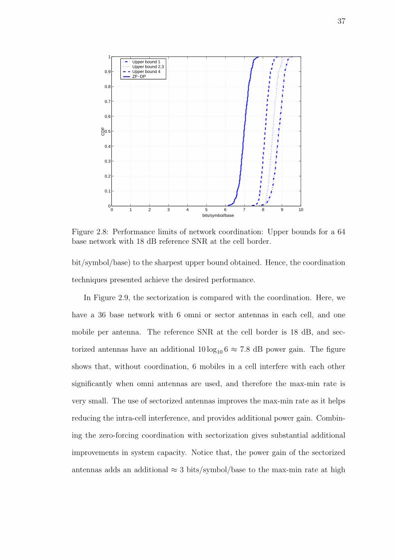
37
0 1 2 3 4 5 6 7 8 9 100
0.1
0.2
0.3
0.4
0.5
0.6
0.7
0.8
0.9
1
CD
F
Upper bound 1Upper bound 2,3Upper bound 4ZF−DP
bits/symbol/base
Figure 2.8: Performance limits of network coordination: Upper bounds for a 64base network with 18 dB reference SNR at the cell border.
bit/symbol/base) to the sharpest upper bound obtained. Hence, the coordination
techniques presented achieve the desired performance.
In Figure 2.9, the sectorization is compared with the coordination. Here, we
have a 36 base network with 6 omni or sector antennas in each cell, and one
mobile per antenna. The reference SNR at the cell border is 18 dB, and sec-
torized antennas have an additional 10 log10 6 ≈ 7.8 dB power gain. The figure
shows that, without coordination, 6 mobiles in a cell interfere with each other
significantly when omni antennas are used, and therefore the max-min rate is
very small. The use of sectorized antennas improves the max-min rate as it helps
reducing the intra-cell interference, and provides additional power gain. Combin-
ing the zero-forcing coordination with sectorization gives substantial additional
improvements in system capacity. Notice that, the power gain of the sectorized
antennas adds an additional ≈ 3 bits/symbol/base to the max-min rate at high

38
0 2 4 6 8 10 120
0.1
0.2
0.3
0.4
0.5
0.6
0.7
0.8
0.9
1ZF− 6 SectorZF− 6 OmniPC− 6 SectorPC− 6 Omni
Figure 2.9: Empirical max-min rate CDFs for a 36 base network with 6 sectorizedor omni transmit antennas, and with 18 dB reference SNR at the cell border.
SNRs. Without the power gain, the coordinated sectorized antennas perform
worse than the coordinated omni antennas. The reason is that the omni antennas
provide mobile-specific beamforming instead of fixed/spatial beamforming, and
have more degrees of freedom for coordination.
In Figure 2.10, the effect of partial channel information is presented in the
context of zero-forcing coordination. We observe that more than half of the
throughput achievable with the full channel information can be obtained when
only the channels of 3− 4 base antennas with the strongest links are available.
2.9 Chapter Summary and Conclusion
Coordinating base antenna transmissions to mitigate inter-cell interference is a
promising idea suggesting large capacity improvements over the conventional cel-
lular networks. Practical concerns regarding the coordination are the need for
39
104 6 128
14
16
2
19
18
0 1 2 3 4 5 6 70
0.1
0.2
0.3
0.4
0.5
0.6
0.7
0.8
0.9
1
bits/symbol/base
CD
F 104 6 128
14
16
2
19
18
# of channel info
1
Figure 2.10: The effect of limited channel information: Empirical max-min rateCDFs for a 64 base network with ZF transmission, and with 18 dB reference SNRat the cell border.
channel knowledge, and a backbone enabling communication between the base
stations, both not far from reach technically. Thus, the network coordination
should be given serious consideration for future wireless networks.

40
Chapter 3
Multiple Antenna Network Coordination
In the previous chapter, we presented network coordination as a means to provide
high spectral efficiency in cellular downlink systems with single antenna units.
Here, we will study the impact of network coordination on multiple antenna
systems. We will show that the coordinated transmissions are especially effective
when the base stations and the mobiles are equipped with multiple antennas.
Without coordination, the link qualities can be very poor because of inter-cell
interference. In this case, the network does not benefit significantly from multiple
antennas since the improvement in rate due to the antenna units is small at low
SNRs. When the coordination is employed, inter-cell interference is mitigated
so that the links can operate in the high SNR regime. This enables the cellular
network to enjoy the great spectral efficiency improvement associated with using
multiple antennas.
3.1 System Model
We consider a cellular network with M base stations, each equipped with t trans-
mit antennas, and N mobiles, each with r receive antennas. All M base stations
can act together, and each user may receive signals from up to tM base antennas.
As in Chapter 2, each base is loaded at most with one user, and also the total

41
number of transmit antennas is assumed to be larger than the total number of
receive antennas, i.e., tM ≥ rN . Taking all the base antennas as input and all
the mobile antennas as output, we have a MIMO network. The received signal
model for the kth mobile is as follows:
yk = Hkx + nk k = 1, 2, . . . , N (3.1)
where yk ∈ Cr×1 is the received signal, Hk = [hij]r×tM denotes the kth user’s
channel matrix with hij being the complex channel gain between the ith receive
antenna and the jth transmit antenna, x ∈ CtM×1 denotes the complex antenna
outputs (without subscript k since it is composed of signals for all N users),
and nk ∈ Cr×1 denotes the white noise vector with covariance σ2Ir. To simplify
our analysis, we redefine the vectors in (3.1) to be in normalized form, meaning
that each vector has been divided by the standard deviation of the additive noise
component, σ. Then, the components of nk have unit variance. Also, the N
vectors {nk}Nk=1 are i.i.d.
The fact that each user has r receive antennas can be exploited in the spatial
domain by transmitting up to r independent symbol streams simultaneously for
each user. Moreover, since all base antennas are coordinated, the complex antenna
output vector x is composed of signals for all N users. Therefore, x can be written
as follows:
x =r∑
j=1
b1jw1j +r∑
j=1
b2jw2j + · · ·+r∑
j=1
bNjwNj (3.2)
where bij denotes the jth symbol of mobile i. In the context of coordinated mul-
tiple antenna transmissions, wij = [w1ij, w
2ij, . . . , w
tMij ]T denotes the complex unit
norm antenna weight vector that is multiplied by bij. The selection of appropriate
42
antenna weight vectors, the mathematical problem, and the solution associated
with each transmission method will be given in the next three sections.
3.2 Multiple Antenna Network Coordination by Zero-Forcing
For the multiple antenna zero-forcing coordination, the antenna weight vectors
are selected so that each user’s data does not interfere with other users’ data. On
the other hand, a user’s own data symbols can interfere with each other. Thus,
each normalized zero-forcing weight vector wij satisfies
Hkwij = 0, ‖wij‖2 = 1, i 6= k, j = 1, . . . , r. (3.3)
In other words, each unit norm weight vector wij has to be orthogonal to the
subspace spanned by other users’ channels. We note that each row of the channel
matrix Hk corresponds to the channel seen by one of the receive antennas of user
k. Let us denote the mth row of the matrix Hk by hkm for m = 1, . . . , r. The
channel vector hkm can be expressed as a sum of two vectors hkm = qkm + q′km
where q′km denotes the part of the vector hkm in the subspace spanned by other
users’ channels. Similarly, we write Hk = Qk + Q′k where qkm and q
′km are the
mth rows of the matrix Qk and Q′k respectively. Notice that the row spaces of
Qk and Q′k are orthogonal spaces. The zero-forcing weight vectors are selected in
such a way that user k’s transmissions do not cause interference to other users,
and therefore are confined into the subspace spanned by the vectors qkm for
m = 1, . . . , r only, or equivalently in the row space of Qk. In order to find the
basis for the row space, we use the singular value decomposition theorem, and
43
write Qk as
Qk = UkSkV†k (3.4)
where Uk ∈ Cr×r and Vk ∈ CtM×tM are unitary, and Sk ∈ Cr×tM is a zero matrix
except for the square roots of r nonzero eigenvalues (r < tM) of the matrix
QkQ†k on the diagonals. We denote each diagonal by λ
1/2kj for j = 1, . . . , r. By
the singular value decomposition theorem, the first r columns of Vk are the bases
for the row space of Qk, and therefore are selected to be the user k’s zero-forcing
weight vectors wkj for j = 1, . . . , r. Using (3.1)-(3.2), and with the particular
selection of zero-forcing weight vectors, the received signal for user k is given by
yk = Hkx + nk (3.5)
= Hk
(r∑
j=1
b1jw1j +r∑
j=1
b2jw2j + · · ·+r∑
j=1
bNjwNj
)+ nk (3.6)
= Hk
(r∑
j=1
bkjwkj
)+ nk (3.7)
= (Qk + Q′k)
(r∑
j=1
bkjwkj
)+ nk (3.8)
= Qk
(r∑
j=1
bkjwkj
)+ nk (3.9)
= UkSkV†k
(r∑
j=1
bkjwkj
)+ nk (3.10)
= Uk
λ1/2k1 bk1
λ1/2k2 bk2
...
λ1/2kr bkr
+ nk (3.11)

44
where (3.7)-(3.9) is due to the fact that each user’s zero-forcing weight vectors are
orthogonal to the subspace spanned by other users’ channels, and (3.11) follows
from the fact that user k’s weight vectors are selected to be the first r columns
of the unitary matrix Vk, and Sk is a diagonal matrix with the square roots of
r nonzero eigenvalues on the diagonals. User k recovers its symbols by match-
filtering the received signal with U†k:
yk = U†kyk =
λ1/2k1 bk1
λ1/2k2 bk2
...
λ1/2kr bkr
+ n (3.12)
where the noise vector nk = U†knk remains white with covariance σ2Ir due to
the unitary transformation. It follows that the rate achievable in the parallel
Gaussian channels (3.12) is given by
Rk =r∑
j=1
log2
(1 + λkjE[|bkj|2]
). (3.13)
Given the antenna weight vector wkj = [w1kj, w
2kj, . . . , w
tMkj ]T , the symbol bkj
with power Pkj = E[|bkj|2] contributes power |wqkj|2Pkj to the total transmit
power at antenna q. The total transmit power at antenna q is the sum of the
contributions of the symbols of all users, i.e.,
Pq =N∑
k=1
r∑j=1
|wqkj|2Pkj. (3.14)

45
Now that we have described how to calculate the achievable rates, and the
individual power constraints at each base antenna, we give the formal problem
statement. The objective is to maximize the minimum rate in the network subject
to per-base (or per-antenna) power constraints. The problem can be defined as
max r0 (3.15)
s.t.r∑
j=1
log2 (1 + λkjPkj) ≥ r0, k = 1, . . . , N (3.15a)
N∑
k=1
r∑j=1
|wqkj|2Pkj ≤ Pmax, q = 1, . . . , tM (3.15b)
r0 ∈ <+, Pkj ∈ <+ ∀ k, j. (3.15c)
Note that r0 can be interpreted as the minimum rate to be maximized, i.e.,
r0 = mink
∑rj=1 log2 (1 + λkjPkj). Also, notice that the constraint in (3.15b)
defines a per-antenna power constraint. However, other types of power constraints
can easily be included in the above optimization problem. For example, if we need
a constraint on the total base power, we need to sum up the contribution of each
base antenna given on the left side of the inequality in (3.15b) and constrain the
sum. In our numerical examples, we will use a per-base power constraint. The
problem (3.15) is a convex optimization problem since the constraints in (3.15b)
are linear, and the constraints in (3.15a) define a convex region. The logarithm
function is concave in the power assignments, and the sum of concave functions is
also concave. Each constraint in (3.15a) defines a convex set, which is the region
underneath a concave function intersected with the region above the hyperplane
defined by r0. This is because the intersection of convex sets is another convex
set. Therefore, standard convex optimization techniques can be used to solve the

46
problem [30].
3.3 Multiple Antenna Network Coordination by Zero-Forcing
Dirty Paper Coding
Similar to the single antenna network coordination schemes, an improved form
of multiple antenna coordination is achieved when zero forcing and dirty paper
coding work together to get rid of the interference. In this section, we will use
a reduced form of zero-forcing to get rid of the interference that the dirty paper
coding does not remove. In the multiple antenna zero forcing coordination, each
user’s interference was nulled out by selecting the weight vectors to be orthogonal
to the other user’s channels. In the dirty paper coding approach, when the inter-
ference is known causally at the transmitter, N users’ codewords can be chosen
such that given an ordering of users [π(1), . . . , π(N)], where π is a permutation,
a user with index π(i) does not suffer any interference from users with lower
indexes, i.e., π(k) with k < i. When dirty paper coding is combined with the
reduced form of zero forcing, the interference still present from dirty paper coding
will be nulled out due to the zero forcing weight vectors. In this case, the weight
vectors for the data symbols of user π(k) with k > i have to be orthogonal to the
user π(i)’s channel. Thus, each zero forcing weight vector wπ(k)j must satisfy
Hπ(i)wπ(k)j = 0, ‖wπ(k)j‖2 = 1, k > i, j = 1, . . . , r. (3.16)
The weight vectors satisfying the above conditions can be found in a similar
way to the zero-forcing case. First, we write the channel vector hπ(k)m as a sum of

47
two vectors hπ(k)m = qπ(k)m + q′π(k)m where q
′π(k)m denotes the part of the vector
hπ(k)m in the subspace spanned by channels of users π(i) with i < k. Similarly,
we write Hπ(k) = Qπ(k) + Q′π(k). The zero-forcing weight vectors are selected in
such a way that user π(k)’s transmissions are confined into the subspace spanned
by the vectors qπ(k)m for m = 1, . . . , r only, or equivalently in the row space of
Qπ(k). In order to find the bases for the row space, we use the singular value
decomposition theorem, and write Qπ(k) = Uπ(k)Sπ(k)V†π(k). The first r columns
of Vπ(k) are selected to be the user π(k)’s zero-forcing weight vectors wπ(k)j for
j = 1, . . . , r. In this case, the received signal for user π(i) is given by
yπ(i) = Hπ(i)x + nπ(i) (3.17)
= Hπ(i)
(r∑
j=1
b1jw1j +r∑
j=1
b2jw2j + · · ·+r∑
j=1
bNjwNj
)+ nπ(i) (3.18)
= Hπ(i)
(r∑
j=1
bπ(i)jwπ(i)j
)+ Hπ(i)
(∑
k>i
r∑j=1
bπ(k)jwπ(k)j
)+ nπ(i)(3.19)
= Hπ(i)
(r∑
j=1
bπ(i)jwπ(i)j
)+ nπ(i) (3.20)
=(Qπ(i) + Q
′π(i)
) (r∑
j=1
bπ(i)jwπ(i)j
)+ nπ(i) (3.21)
= Qπ(i)
(r∑
j=1
bπ(i)jwπ(i)j
)+ nπ(i) (3.22)
= Uπ(i)Sπ(i)V†π(i)
(r∑
j=1
bπ(i)jwπ(i)j
)+ nπ(i) (3.23)
= Uπ(i)
λ1/2π(i)1bπ(i)1
λ1/2π(i)2bπ(i)2
...
λ1/2π(i)rbπ(i)r
+ nπ(i) (3.24)

48
Input : Hk = [hij]r×tM , k = 1, 2, . . . , N (channel response matrices).Output : π = [π(1), π(2), . . . , π(N)], (π(i) projects away from π(j) where i > j).Initialization : S = {1, 2, . . . , N}.for k = 1 : N
π(k) = arg mink∈S log2
[det(Ir + PmaxHkH
†k)
],
S = S− π(k),
eπ(k),i =hπ(k),i
|hπ(k),i| , i = 1, . . . , r, (hπ(k),i : ith column of Hπ(k))
hj,l = hj,l − (h†j,leπ(k),i)eπ(k),i, ∀j ∈ S, i, l = 1, . . . , r.end
Figure 3.1: The heuristic user-ordering algorithm for multiple antenna networks.
where (3.19) follows from the fact that a user with index π(i) does not suffer
any interference from users π(k) with k < i due to the dirty paper coding. The
interference that dirty paper coding cannot get rid of, i.e., the term inside the
second parenthesis in (3.19), is nulled out by appropriate zero forcing weight
vectors (3.16), and accordingly (3.20) represents the received signal after both
dirty paper coding and zero-forcing. Equation (3.22) is due to the fact that the
weight vector wπ(i)j is a basis in the row space of the matrix Qπ(i), which is
orthogonal to the row space of Q′π(i). The remaining steps are due to the singular
value decomposition theorem.
Given the received signal (3.24), the calculation of the achievable rates, and
the power constraints at each base follow the same steps as in the previous section.
Similarly, the problem statement is the same as (3.15), except that the eigenvalues
and the weight vectors have to be determined based on the zero-forcing dirty paper
coding scheme described in this section.
The above multiple antenna network coordination scheme assumes a particular
user ordering. In this case, a similar version of the heuristic we mentioned in the
context of single antenna systems can be used. Namely, the user with the smallest
single-user log-det capacity is a disadvantaged user. Since the objective is fairness,

49
all other users have to project away from this user. In turn, the disadvantaged
user “pays the favor back” by being invisible via the dirty paper encoding. In
the subspace that does not cause interference to this disadvantageous user, the
next user with the smallest log-det capacity is chosen to be the second user in the
ordering. These steps are followed in the same way for the remaining mobiles.
The heuristic user ordering algorithm is shown in Figure 3.1. We will see in the
numerical examples section that the algorithm performs quite well in our cellular
network setup.
3.4 Multi-antenna Cellular Networks with Power Control
Our baseline for comparison with the coordinated schemes is a conventional mul-
tiple antenna cellular network with power control. As an extension of the single
antenna power control scheme, we will assume a simple form of power control
where each antenna of a base station transmits with the same power Pk, and the
power level at each base is controlled. We also assume that xk is Gaussian with co-
variance PkIt. In this case, user k’s rate is given by log2
[det(Ir + PkHkH
†kR
−1)]
where R =∑N
i=1,i6=k PiHiH†i +Ir. To maximize the minimum rate in the network,
we solve the following problem
max r (3.25)
s.t. log2
[det(Ir + PkHkH
†k(
N∑
i=1,i 6=k
PiHiH†i + Ir)
−1)
]≥ r, k = 1, . . . , N
(3.25a)
0 ≤ Pk ≤ Pmax, r ∈ <+. (3.25b)

50
The way we approach this problem is also analogous to the power control
problems in single-antenna systems [37, 38]. First, we start with a very low,
easily achievable target rate r, and initialize all power assignments to zero. Next,
we determine the power level for each user to achieve the target rate given the
interference of other users. In the second iteration, we increase the target rate, and
given the set of power assignments from the previous iteration and corresponding
interference levels, we calculate the new set of power levels to achieve the new
target rate. We follow the same procedure, with higher target rates, until any
of the base station power constraints is violated. By the very nature of this
procedure, the successive iterations generate a bounded sequence of increasing
rates, and therefore the method converges.
3.5 Performance Evaluation
In this section, we will compare the performance of coordinated multiple antenna
networks to that of conventional cellular networks with inter-cell interference. In
Chapter 2, we showed that the coordination is successful in eliminating inter-cell
interference. Our results in this section indicate that the coordination does more
than mitigate the inter-cell interference. Namely, the coordination improves the
effectiveness of multiple antennas in cellular networks.
Our basic experimental setup is the same as in Chapter 2. In particular, each
base is located at the center of one of the 64 hexagonal cells whose sample layout
is shown in Figure 2.3. We denote by (t, r) a configuration in which each base
station has t transmit antennas and each mobile has r receive antennas. Three
antenna configurations will be considered: (1,1), (2,2) and (4,4) where the base

51
0 2 4 6 8 10 120
0.1
0.2
0.3
0.4
0.5
0.6
0.7
0.8
0.9
1
CD
F
bits/symbol/base
(1,1)(2,2)(4,4)
Figure 3.2: Empirical max-min rate CDFs: Multiple antenna power control resultsfor a 64 base network.
0 5 10 15 20 25 300
0.1
0.2
0.3
0.4
0.5
0.6
0.7
0.8
0.9
1
CD
F
bits/symbol/base
(1,1)(2,2)(4,4)
Figure 3.3: Empirical max-min rate CDFs: Multiple antenna zero-forcing resultsfor a 64 base network.

52
0 5 10 15 20 25 300
0.1
0.2
0.3
0.4
0.5
0.6
0.7
0.8
0.9
1
CD
F
bits/symbol/base
(1,1)(2,2)(4,4)
Figure 3.4: Empirical max-min rate CDFs: Multiple antenna zero-forcing dirtypaper coding results for a 64 base network.
stations and the mobiles are equipped with 1, 2 and 4 antennas respectively.
Each base is loaded with one mobile, and 10% of the mobiles are allowed to be
in outage. We assume path-loss with a 3.8 propagation exponent, log-normal
shadowing with 0 mean and 8 dB standard deviation, and Rayleigh fading for
each transmit/receive antenna pair with 0 mean, unit variance complex Gaussian
component. Given a maximum base power of 10 W, a mean power loss of 134 dB
at the reference distance of 1.6 km from the base, a receiver noise figure of 5 dB,
a vertical antenna gain of 10.3 dBi, a channel bandwidth of 5 MHz, and a receiver
temperature of 300oK, the SNR at the reference distance is 18 dB (considering
one transmit/receieve antenna pair), accounting only for path loss and ignoring
shadowing and Raleigh fading. However, because of inter-cell interference, the
SINR can fall below 0 dB in our network setup.
We have seen in the previous chapter that, for cellular networks with single

53
30
(1,1) (2,2) (4,4)
Power Control
Zero Forcing
Dirty Paper Coding
25
bit
s/s
ec/H
z/b
ase
20
15
10
5
0
(# of Transmit antennas per base, # of Receive antennas per user)
Figure 3.5: Spectral efficiency v.s. # of antennas.
Figure 3.6: Summary of the multiple antenna results. The results for a conven-tional network with each base antenna transmitting at the maximum power limitis also presented.
54
antenna terminals, the coordination improves the max-min rate of the network by
about a factor-of-3 when the zero-forcing coordination is employed, and by about
a factor-of-5 when the combined zero-forcing dirty paper coding scheme is used.
Corresponding multiple antenna spectral efficiency results obtained by averaging
over many network instances are shown in Figure 3.2-3.6 for all three antenna
arrangements. The figure shows that the use of multiple antennas improves (lin-
early) the spectral efficiency of the network for all transmission methods. How-
ever, the gain in terms of the marginal increase in rate when an additional an-
tenna is deployed is small without coordination. We observe in Figure 3.5 that
the slope of the rate versus the number of antennas curve is small for the uncoor-
dinated transmissions with power control, while it is significantly improved when
the coordination is employed. More than a factor-of-10 improvement in spectral
efficiency is reported due to both network coordination and (4, 4) antenna ar-
rangements compared to the baseline of uncoordinated transmissions with single
antenna terminals. The results show that the removal of “out of cell” interference
greatly enhances the spectral efficiency improvement associated with increasing
the number of antennas.
3.6 Chapter Summary and Conclusion
In this chapter, we have considered multiple antenna cellular networks with and
without network coordination. We have seen that the network suffers from inter-
cell interference when the coordination is not employed, and this would reduce the
effectiveness of multiple antennas due to relatively low link SNRs. On the other
hand, employing network coordination improves the link qualities, and enables

55
the cellular network to realize the predicted capacity improvement due to the
multiple antennas. This suggests that if the multiple antennas are to be deployed
in a practical interference-limited cellular downlink system, it is necessary to
employ some form of interference mitigation technique to improve link SNRs.
The network coordination is an effective way of achieving this objective.

56
Chapter 4
Beamforming Design With Per-Antenna Power
Constraints
Thus far, we have considered coordination techniques that require simple, prac-
tical linear beamforming techniques. For the single antenna zero-forcing method,
each mobile’s data symbol is multiplied by a beamforming vector given by the col-
umn of the pseudo-inverse matrix. Similarly, for the combined zero-forcing dirty
paper coding scheme with single antenna terminals, the beamforming vectors are
given by the columns of the unitary matrix obtained by the LQ decompositions of
the channel matrix. Both derivations are extended to the multiple antenna sys-
tems as well. While these linear beamforming techniques provide significant ca-
pacity improvements over the conventional cellular networks, they are not claimed
to be the optimal linear coordination techniques. The objective in this chapter is
to find the optimal beamforming vectors for the coordinated transmissions.
Notice that, in our problem formulations, each base station antenna has a
separate power constraint. The optimal system design with per-antenna power
constraints is different than the design based on a sum-power constraint. This
fact can be illustrated by a simple example where M transmit antennas serve one
mobile with a single antenna. Let’s assume that the mobile’s i.i.d. vector channel
is denoted by h = [h1, h2, . . . , hM ]T , and the antenna outputs are denoted by
x = [x1, x2, . . . , xM ]T . When the system is sum-power constrained, the optimal

57
transmission method is the transmit beamforming where the antenna outputs
are aligned with the mobile’s channel, and the beamforming vector is scaled to
the maximum transmit power P . Thus, the optimum antenna output becomes
xopt = Ph†/|h|. When each antenna has a separate power constraint, say P′=
P/M for each antenna, the optimum transmission method is to transmit full
power at each antenna, and phase-match the output voltages to the channels,
i.e., xopt = P′[h†1/|h1|, h†2/|h2|, . . . , h†M/|hM |]T . The problem with the transmit
beamforming in this case is that it gives more weights to the antennas whose
channels are good, and in the case of a per-antenna power constraint, this makes
the antenna power to drain quickly.
So far, our beamforming design ignores the existence of a per-antenna power
constraint, and therefore is similar to the transmit beamforming design. For ex-
ample, when the pseudo-inverse matrix is used for the zero-forcing, each mobile’s
beamforming vector becomes aligned with the part of the mobile’s channel which
does not deposit interference on the others. Similarly, for the multiple antenna
zero-forcing system, beamforming vectors are chosen to be the eigenvectors of
the part of the mobile’s channel matrix which is orthogonal to the others. No-
tice that, despite ignoring the existence of per-antenna power constraints, these
beamforming designs performed quite well as their performance gets very close
to the upper bounds obtained in Chapter 2. The reason is that, as we will see
in the following sections, optimizing the antenna outputs based on per-antenna
power constraints may improve the rate considerably when the number of trans-
mit antennas is much larger the number of receive antennas, i.e., tM À rN in
the multiple antenna system and tM À N in the single antenna system. This is
because more transmit antennas will give more degrees of freedom to optimize the

58
antenna outputs. When the number of transmit and receive antennas are close to
each other, there are not much room left to exploit in the signal space (consider
the zero-forcing design where each mobile’s transmission has to be projected away
from the others), which is the case in the previous two chapters.
4.1 System Model
We consider a broadcast system with a transmitter equipped with M antennas,
and N mobiles, each with a single receive antenna. The received signal model for
the kth mobile is as follows:
yk = h†kx + nk k = 1, 2, . . . , N (4.1)
where yk is the received signal, hk = [hk1, hk2, . . . , hkM ]† denotes the kth mobile’s
complex channel vector, x = [x1, x2, . . . , xM ]† denotes the antenna outputs (with-
out subscript k since it is composed of signals for all N mobiles), and nk denotes
the complex Gaussian noise with variance σ2. In the above model, the M transmit
antennas can be thought of as multiple transmit antennas of a base station in a
single cell system, or alternatively as a network-wide transmit antenna array in a
multi-cell system when M base stations are connected via a high-speed backbone
enabling coordinated base transmissions.
We assume that the transmitter employs linear beamforming where the vector
wk = [wk1, wk2, . . . , wkM ]† is used to map the kth mobile’s data symbol bk to the
antenna outputs. The antenna output x is composed of signals for all N mobiles,

59
and therefore is given by
x =N∑
k=1
bkwk. (4.2)
As a case study, we are interested in the zero-forcing beamforming where
each mobile’s transmissions do not cause interference to others. Our analysis can
simply be extended to the zero-forcing dirty paper coding system design as well.
In the zero-forcing case, the beamforming vector wk is chosen to be orthogonal
to all other mobiles’ channels:
h†jwk = 0, j 6= k. (4.3)
Given the requirement (4.3), and using (4.2), the kth mobile’s received signal
with zero-forcing beamforming becomes yk = bkh†kwk + nk. Assuming that the
data symbol bk is zero-mean Gaussian with unit variance, mobile k’s achievable
rate is given by
rk = log2
(1 +
|h†kwk|2σ2
). (4.4)
Finally, each transmit antenna has a power constraint given by E[|xm|2] ≤
Pmax, m = 1, . . . ,M . Since the data symbols for different mobiles are i.i.d., this
constraint can be written as∑N
k=1 |wkm|2 ≤ Pmax, m = 1, . . . , M .
4.2 Problem Formulation and Solution
The objective is to design a zero-forcing beamforming system so as to maximize
the minimum rate in the network subject to per-antenna power constraints. The

60
optimization problem can be written as
maxwk
r0 (4.5)
s.t. log2
(1 +
|h†kwk|2σ2
)≥ r0, k = 1, . . . , N, (4.5a)
N∑
k=1
|e†mwk|2 ≤ Pmax, m = 1, . . . ,M, (4.5b)
h†jwk = 0 ∀j 6= k, wk ∈ CM×1, r0 ∈ <+. (4.5c)
where em is a standard basis vector which has 1 for its mth component, and 0
for every other component. In the above formulation, r0 can be interpreted as
the minimum rate to be maximized, i.e., r0 = mink log2(1 + |h†kwk|2/σ2). First,
notice that the zero-forcing constraints in (4.5c) are simply linear. Moreover,
the per-antenna power constraints (4.5b) define a convex set, since the function
f(wk) = |e†mwk|2 is convex in wk, the sum of convex functions is convex, and α-
sublevel set of a convex function defined by {wk ∈ dom f | f(wk) ≤ α} is a convex
set [30]. The rate constraints (4.5a) can be written as |h†kwk| ≥√
(2r0 − 1)σ2,
k = 1, . . . , K, which defines a non-convex set since it is the region outside of
a convex set defined by |h†kwk| ≤√
(2r0 − 1)σ2. Therefore, the problem above
is not a convex optimization problem, for which a tractable analytical solution
would be possible.
Fortunately, the problem can be simplified significantly by observing that
the optimum beamforming vectors are invariant to phase-shifts, i.e., if w∗k is an
optimum beamforming vector for the problem (4.5), then the vector ejθw∗k is also
an optimum beamforming vector [33, 34]. This is because of the fact for any
feasible wk, the vector ejθwk would also satisfy the constraints (4.5a)-(4.5c). In

61
this case, without loss of generality, we can search for the optimum beamforming
solutions among the vectors that would result in positive and real projections
h†kwk. Thus, an equivalent optimization problem can be written as
maxwk
t (4.6)
s.t. (h†kwk) ≥ t, k = 1, . . . , N, (4.6a)
Im(h†kwk) = 0 ∀k, (4.6b)
K∑
k=1
|e†mwk|2 ≤ Pmax, m = 1, . . . ,M, (4.6c)
h†jwk = 0 ∀j 6= k, wk ∈ CM×1, t ∈ <+. (4.6d)
where t =√
(2r0 − 1)σ2, and the optimum beamforming vectors maximizing t
would also maximize r0. Similar to (4.5), the constraints (4.6c) and (4.6d) are
convex and linear respectively, and (4.6a) and (4.6b) are linear constraints. Since
the objective function is also linear, the problem (4.6) is a convex optimization
problem.
In the next section, we will consider the conventional zero-forcing technique
based on the Moore-Penrose pseudo-inverse, and investigate why and when this
technique can be an optimal/suboptimal solution to the above problem (4.6).
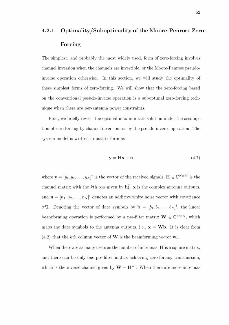
62
4.2.1 Optimality/Suboptimality of the Moore-Penrose Zero-
Forcing
The simplest, and probably the most widely used, form of zero-forcing involves
channel inversion when the channels are invertible, or the Moore-Penrose pseudo-
inverse operation otherwise. In this section, we will study the optimality of
these simplest forms of zero-forcing. We will show that the zero-forcing based
on the conventional pseudo-inverse operation is a suboptimal zero-forcing tech-
nique when there are per-antenna power constraints.
First, we briefly revisit the optimal max-min rate solution under the assump-
tion of zero-forcing by channel inversion, or by the pseudo-inverse operation. The
system model is written in matrix form as
y = Hx + n (4.7)
where y = [y1, y2, . . . , yN ]† is the vector of the received signals, H ∈ CN×M is the
channel matrix with the kth row given by hTk , x is the complex antenna outputs,
and n = [n1, n2, . . . , nN ]† denotes an additive white noise vector with covariance
σ2I. Denoting the vector of data symbols by b = [b1, b2, . . . , bN ]†, the linear
beamforming operation is performed by a pre-filter matrix W ∈ CM×N , which
maps the data symbols to the antenna outputs, i.e., x = Wb. It is clear from
(4.2) that the kth column vector of W is the beamforming vector wk.
When there are as many users as the number of antennas, H is a square matrix,
and there can be only one pre-filter matrix achieving zero-forcing transmission,
which is the inverse channel given by W = H−1. When there are more antennas

63
than users, the pre-filter matrix takes the form of a pseudo-inverse matrix given
by W = H†(HH†)−1. Geometrically speaking, in both cases, each user’s channel
is projected away from all other users’ channels, and the remaining piece of the
channel gives the beamforming direction which would not cause interference to
others. When the above pre-filter matrices are used, each user receives its own
data symbol corrupted by the noise, i.e., yk = bk + nk. Denoting the power of
bk by pk = E[|bk|2], the following convex problem results in the max-min rate
solution for the given pre-filter matrix W:
maxpk
r0 (4.8)
s.t. log2
(1 +
pk
σ2
)≥ r0, k = 1, . . . , N , (4.8a)
|W11|2 . . . |W1N |2...
...
|WM1|2 . . . |WMN |2
p1
...
...
pN
≤ Pmax1, (4.8b)
r0, pk ∈ <+ (4.8c)
In the above problem, (4.8b) represents the per-antenna power constraints,
and is obtained using the fact that the antenna powers are on the diagonals of
the following transmit covariance matrix
E[xx†] = WE[bb†]W† = W
p1
. . .
pN
W†, (4.9)
64
h3
..
h2: mobile 2’s channel
h1: mobile 1’s channel
Figure 4.1: 3 transmit antennas and 2 mobiles with orthogonal channels.
and the constraints on the diagonals can be expressed in the matrix form (4.8b).
We will show in the case of 2 users that, when there is a sum-power constraint
instead of a per-antenna power constraint (4.5b), the columns of the Moore-
Penrose pseudo-inverse matrix defines the optimum beamforming directions, and
the above problem (4.8) would result in the max-min rate solution for the original
problem (4.5). On the other hand, the same zero-forcing form is suboptimal when
there are per-antenna power constraints.
Proposition 1. The beamforming based on the Moore-Penrose pseudo-inverse
matrix W = H†(HH†)−1 is a suboptimal form of zero-forcing when there are
per-antenna power constraints.
Proof. We prove the statement by an example. Consider a broadcast system with
3 transmit antennas and 2 single antenna mobiles with channels h1,h2 ∈ C3×1.
Assume that h1 and h2 are orthogonal, h†1h2 = 0. In three dimensional space,
there is a third vector h3 ∈ C3×1, which is orthogonal to both h1 and h2. These
three vectors are shown in Figure 4.1. The matrix H ∈ C2×3 representing the
channel between the two mobile antennas and the transmit antenna array has hT1
65
and hT2 on its rows. The zero-forcing beamforming directions are on the column
vectors of the pseudo-inverse channel H†(HH†)−1, and are given by h1/|h1|2 and
h2/|h2|2 respectively. In this case, the signals are transmitted in the directions
of h1 and h2 intended for the first and the second mobile respectively. These
particular beamforming selections make sense since they provide interference-free
transmission because h†1h2 = 0, and any signal transmitted in the direction of
h3 cannot add up rate for neither mobiles. However, we will show that the third
orthogonal dimension h3 is in fact useful.
Let us write the antenna outputs as
x = b1
√P1w1 + b2
√P2w2 + b3
√P3w3 (4.10)
where Pk is the transmit power associated with zero-mean unit-variance data
symbol bk, and wk = hk/|hk| is the unit-power beamforming vector. If no sig-
nal is transmitted in the direction of h3, then P3 = 0 which is the case with
the pseudo-inverse zero-forcing. If b3 is chosen to be an independent data sym-
bol, then the total transmit power at the mth antenna is∑3
k=1 Pk|e†mwk|2, and
clearly P3 is wasted as b3 cannot be received by neither mobiles (w3 is orthogonal
to both h1 and h2). The only remaining option is to transmit either b1 or b2
(or a linear combination of them) in the third orthogonal dimension. For exam-
ple, if b3 = b1, then the total transmit power at the mth antenna is given by
P2|e†mw2|2 + |e†m(√
P1w1 +√
P3w3)|2. This shows that, although transmitting b1
in the direction of h3 cannot add up rate for mobile 1, it affects the power con-
straint, and may even help to save some power by coherently nulling out transmit
voltage at an antenna.

66
For example, assume two orthogonal mobile channel vectors h1 = (0, 2, 0)
and h2 = (0.8, 0, 0.6). In this case, the third orthogonal dimension is given by1
h3 = (0.6, 0,−0.8). When the pseudo-inverse zero-forcing is used, the unit-norm
beamforming vectors are given by w1 = (0, 1, 0), w2 = (0.8, 0, 0.6), and
xzf = b1
√P1w1 + b2
√P2w2. (4.11)
Assuming that Pmax = 1 W, the max-min received power is Pmax/(0.8)2 ∼= 1.56
W, which is achieved when P1∼= 0.39 W, P2
∼= 1.56 W. Notice that the power
constraint is active only for the first transmit antenna. Instead, the following
signal can be transmitted
x′= b1
√P′1w1 + b2
√P′2(1.4w2 − 0.2w3), (4.12)
where w3 = (0.6, 0,−0.8), P′1 = 0.49 W and P
′2 = 1 W. In this case, the third
orthogonal dimension is used to send the second mobile’s data, which helps to
increase the max-min rate received power to 1.96 W. This improvement can be
explained in two ways. First, the first and the third antennas transmit at full
power in this case, which improves the second mobile’s received power. Second,
more power is transmitted in the direction of the second mobile’s channel h2, and
the beamforming direction w2. This would not be feasible without w3, since the
power constraint at the first antenna would be violated. Sending signal on w3
has the effect of nulling out part of the transmit voltage on the first antenna, and
1This particular numerical example is given for its simplicity, and is not intended to representrealistic channel realizations. Also, the channel values include both the magnitude and the phasecomponents, and therefore can be negative depending on its phase.

67
therefore easing the power constraint.
Theorem 1. The beamforming based on the Moore-Penrose pseudo-inverse ma-
trix W = H†(HH†)−1 is the optimal form of downlink zero-forcing beamforming
when the system is sum-power constrained.
Proof. We will prove the theorem in the case of 2 users with single antenna
receivers. The same result can be extended to multiple users as well. We have to
show that each mobile’s beamforming vector obtained by the pseudo-inverse zero-
forcing corresponds to the part of the mobile’s channel orthogonal to the other
mobiles’ channels. The optimality of the pseudo-inverse zero-forcing follows from
the fact that, subject to a sum power constraint, the transmit beamforming is
optimal, and therefore there is no need to transmit any signal in any direction
that would not contribute to the data rate.
First, notice that the (i, j)th entry of the matrix HH† is given by hTi hj, which
is the projection of the ith mobile’s channel onto the jth mobile’s channel. For
the 2 user case, its inverse matrix is given by
(HH†)−1 =1
|h1|2|h2|2 − (hT1 h2)2
|h2|2 −hT1 h2
−hT1 h2 |h1|2
(4.13)
The first column of the matrix W = H†(HH†)−1 is the beamforming vector
w1 used to transmit the data symbol b1 (similarly, w2 for b2). Since the kth
column of H† is hk, it follows that
w1 =|h2|2
|h1|2|h2|2 − (hT1 h2)2
(h1 − hT
1 h2
|h2|h2
|h2|)
. (4.14)
68
The term inside the parenthesis in (4.14) is the part of h1 that is orthogonal to
h2. In M -dimensional space, there is a subspace defined by M − 2 basis vectors,
which are orthogonal to both w1 and h2, and therefore can be used to transmit
the data symbol b1 without violating zero-forcing constraints (without causing
interference to the second mobile). Thus, the optimal beamforming vector for the
first mobile can be in the following form
wopt = α1w1 +∑
∀ek⊥w1,h2
αkek (4.15)
where ek is a basis vector in the subspace orthogonal to w1 and h2, and for
some α1, αk ∈ <. Notice that only the signal transmitted in the direction of
w1 can be received by the first mobile. Moreover, when the sum-power is a
concern, any signal transmitted in the direction of ek would be a waste since
E[|b1wopt|2] = p1α21|w1|2 + p1
∑∀ek⊥w1,h2
α2k|ek|2 where p1 = E[|b1|2], and the
second term in the sum does not contribute to the received power. Thus, the
signal intended for the first mobile must be transmitted in the direction of w1,
which is the beamforming direction chosen by the pseudo-inverse zero-forcing.
The same analysis applies to the second mobile as well.
4.3 Performance Evaluation
In this section, we will compare the performance of the optimum zero-forcing
design with that of the zero-forcing based on the Moore-Penrose pseudo-inverse
when there are per-antenna transmit power constraints. We will see that the
pseudo-inverse zero-forcing performs increasingly worse compared to the optimum
design as the number of transmit antennas increases.

69
Our basic experimental setup is as follows. We consider a downlink network
where the transmitter is equipped with multiple antennas, and each mobile has
a single receive antenna. This model is valid for a single cell system with mul-
tiple transmit antennas at the base station, or a multi-cell system with single
or multiple antenna base stations. Each transmit antenna is assumed to have a
separate power constraint. We evaluate the performance improvement due to the
optimum beamforming design in a single-cell system. The total base transmit
power is constrained to 10 Watts, and in the case of t transmit antennas, each
antenna power will be constrained to 10/t Watts. We assume path-loss with a 3.8
propagation exponent, log-normal shadowing with 0 mean and 8 dB standard de-
viation, and Rayleigh fading for each transmit/receive antenna pair with 0 mean,
unit variance complex Gaussian component. Given a mean power loss of 134 dB
at the reference distance of 1.6 km from the base, a receiver noise figure of 5 dB,
a vertical antenna gain of 10.3 dBi, a channel bandwidth of 5 MHz, and a receiver
temperature of 300oK, the SNR at the reference distance is 18 dB (considering
one transmit/receieve antenna pair), accounting only for path loss and ignoring
shadowing and Raleigh fading.
Figure 4.2 compares the spectral efficiency (averaged over many random net-
work realizations) of the optimum zero-forcing and the pseudo-inverse zero-forcing
in the case of a 2 user system. When there are only 2 transmit antennas, there
is only one way of achieving the zero-forcing transmission, which is given by the
channel inversion. In this case, the optimum zero-forcing design and the pseudo-
inverse design have the same spectral efficiency. On the other hand, the optimum
design becomes increasingly better compared to the pseudo-inverse design when

70
0 2 4 6 8 10 12 14 16 18 204
5
6
7
8
9
10
# of transmit antennas
bits
/sec
ond/
Hz
Optimum zero−forcing beamformingPseudo−inverse zero−forcing
Figure 4.2: Optimum zero-forcing beamforming vs. Moore-Penrose pseudo-inverse zero-forcing: 2 users with single antenna receivers.
the number of transmit antennas increases, as it effectively uses available sig-
nal space to optimize the antenna outputs, and to reduce the transmit power at
particular antennas with limited transmit power, while the pseudo-inverse zero-
forcing does not have the same capability. Notice that, according to Figure 4.2,
the optimum zero-forcing design requires only 8 transmit antennas to achieve a
target spectral efficiency of 8 bits/second/Hz, while the pseudo-inverse design re-
quires 16 transmit antennas for the same spectral efficiency. Figures 4.3 and 4.4
also support similar conclusions in the case of 4 users and 8 users respectively.

71
0 2 4 6 8 10 12 14 16 18 20 222
3
4
5
6
7
8
bits
/sec
ond/
Hz
Optimum zero−forcing beamformingPseudo−inverse zero−forcing
# of transmit antennas
Figure 4.3: Optimum zero-forcing beamforming vs. Moore-Penrose pseudo-inverse zero-forcing: 4 users with single antenna receivers.
4.4 Chapter Summary and Conclusion
In this chapter, we studied the optimum zero-forcing beamforming design with
per-antenna power constraints. We observe that the optimum beamforming vec-
tors are invariant to the phase-shifts. This observation helps us to formulate
convex optimization problems finding the optimum vectors. Our numerical re-
sults indicate that optimizing the antenna outputs based on the per-antenna
constraints improves the rate when the number of transmit antennas is larger
the number of receive antennas. In this case, the additional degrees of freedom
given by more transmit antennas helps the per-antenna power constraints. In
particular, the additional degrees is used to null out part of the transmit voltages
at particular antennas with relatively high transmit powers. Our analysis can be

72
0 5 10 15 20 251
2
3
4
5
6
7
# of transmit antennas
bits
/sec
ond/
Hz
Optimum zero−forcing beamformingPseudo−inverse zero−forcing
Figure 4.4: Optimum zero-forcing beamforming vs. Moore-Penrose pseudo-inverse zero-forcing: 8 users with single antenna receivers.
extended to improve the performance of the zero-forcing scheme in the combined
zero-forcing dirty paper coding technique of the previous two chapters. Also, we
plan to extend our analysis to downlink networks with multiple antenna receivers.
73
Chapter 5
Cellular Backhaul Design to Enable
Communication and Coordination Between the
Base Stations
The techniques of the previous chapters assume the existence of a high-speed
backhaul enabling communications between the base stations. In this chapter, we
study the design of such a backhaul in a cellular network. More specifically, we
consider a mesh backhaul network consisting of fixed base stations (mesh routers)
connected by wireless links. Some of the mesh routers have connections to the
wired network, and therefore can function as gateways. The network has multi-
hop capability where the traffic entering the mesh backhaul through the gateway
routers can be carried over multiple wireless links towards the destination mesh
routers. The objective in this work is to study the capacity of such networks.
Assuming the use of an OFDMA air-interface for the mesh backhaul network, we
formulate a cross-layer optimization problem that involves power control, channel
allocation, link scheduling and routing. Our results indicate that OFDMA-based
mesh architecture provides an efficient backhaul solution in cellular networks.

74
5.1 Introduction
Next generation wireless networks are designed to provide broadband services
with quality of service (QoS) support for various applications including voice and
multimedia data. The successful deployment of these all-IP networks requires
advanced network architectures with high spectral efficiency, ubiquitous cover-
age and cross-layer optimized system design. To achieve these goals, a service
provider may deploy a large number of access points (base stations) in a given
service area. On the other hand, the cost of connecting these base stations by
a wired backhaul is too high, mainly because of the cable deployment cost. In
this case, a wireless backhaul is necessary to enable communications between the
base stations. As an efficient backhaul architecture, wireless mesh network is a
promising system design providing interoperability among different wireless tech-
nologies including Wi-Fi and 3G, and its all-IP network design enables extended
network coverage through multi-hop routing. In this study, we consider a mesh
network backhaul architecture for a cellular system, and investigate how a mesh
backhaul can improve the cellular network coverage and the capacity.
In our network architecture, we assume the use of an OFDMA air-interface
for the mesh backhaul. In this case, the wideband channel available in each base-
to-base link is divided into narrowband subchannels, called tones, for efficient use
of spectrum in multipath environments. Our objective is to optimize the radio
resources, such as transmit power and tone allocations, and study efficient routing
and scheduling techniques so as to maximize the end-user throughput. As we
will see, this problem is relatively complex because of the non-linear constraints
involved, and the size of a typical network; hence a large number of parameters
involved (flow control, link scheduling, tone and power allocations for every link
75
in the network). However, the base locations are fixed, and therefore the channels
are relatively static and time-invariant. This fact can be used to perform network
optimization in an off-line fashion.
Wireless mesh networks have been studied extensively in the literature. A
survey paper summarizing the recent state of art, and open research issues can
be found in [39]. A mesh architecture in a cellular network context has been
considered in [40]. Given a set of scheduling modes (sets of simultaneously active
links), and assuming constant transmit power, a linear programming framework
is used to optimize the throughput. Joint routing and scheduling schemes have
been studied to characterize the capacity of mesh networks in [41–43]. Assuming
constant link capacities and no power control, and by modeling the link schedul-
ing feasibility as an explicit constraint in the optimization problem, the authors
develop efficient algorithms to find the set of achievable rates in multi-hop wireless
networks. We will use the same scheduling constraint in our problem formulation
to determine the set of simultaneously active OFDM tones. Joint power control,
scheduling and/or routing in multi-hop adhoc networks is considered in [44–47].
In [44], average power consumption of a link is calculated by taking into account
of the fraction of time the link is scheduled to be active. We will use a similar
model to define the mesh node power constraints in an OFDMA network. Among
the joint power control, scheduling and/or routing problems studied in the litera-
ture, [44,46] are closest to our work. The analysis in both [44,46] apply to single
carrier systems. In the case of a single-carrier system, when a link between two
nodes with bandwidth W is active, the whole bandwidth W is used for transmis-
sion. In the case of multi-carrier systems, the link between the same two nodes
can be partially utilized by using a fraction of the bandwidth W (preferably part

76
of the spectrum with favorable channel conditions) for transmission. This enables
more efficient use of spectrum in the mesh backhaul. Moreover, our scheduling
model is more constrained than the model in [46] in the sense that we impose
per-tone level half-duplex and multi-access/broadcast constraints as we will ex-
plain in more detail in Section 5.2.3. Comparison of different routing metrics and
protocols in multi-hop wireless networks has been studied in [48, 49]. Capacity
limits of adhoc networks and their scaling laws are investigated in [50,51].
Our main contribution in this study is the analysis of the use of an OFDMA
type air-interface [52] in wireless mesh networks. To the best of our knowledge,
this is the first study conducting a detailed analysis of the use of OFDMA in a
mesh backhaul. By providing multiple orthogonal channels in each link, OFDMA
provides multi-radio advantage with a single radio in mesh networks. Moreover,
when the radio resources are optimized carefully, OFDM transmissions may pro-
vide tone-diversity advantage in the form of efficient bandwidth utilization by
choosing better channels for transmissions and scheduling, or in the form of im-
proved routing performance by providing more path options to route the traffic.
To study the performance limits of OFDMA mesh backhaul, and to find effi-
cient algorithms achieving these performance limits, we formulate a cross-layer
optimization problem involving power control, OFDMA resource allocation, link
scheduling and routing. Using our framework, we quantify the throughput of a
mesh backhaul in realistic cellular environments.
The outline of the study is as follows. In Section 5.2, we describe the system
model, and explain transmission constraints in the physical layer, scheduling con-
straints in the link layer, and flow constraints in the routing layer. Cross-layer

77
Figure 5.1: A sample network topology.
throughput optimization problem is defined in Section 5.3. The problem of iden-
tifying individual routing paths achieving the optimal throughput is studied in
Section 5.4. Simulation setup, and the numerical results are given in Section 5.5.
We conclude the study, and give future research directions in Section 5.6.
5.2 System Model
We consider the backhaul of a mesh network consisting of fixed base station
routers connected by wireless links. Some of the mesh routers have connections
to the wired network, and therefore can function as gateways. The network has
multi-hop capability where the traffic entering the network through the gateway
routers can be carried over multiple mesh-to-mesh wireless links towards the des-
tination mesh client. The objective in this work is to study the capacity of such
networks.
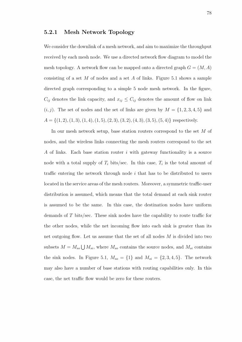
78
5.2.1 Mesh Network Topology
We consider the downlink of a mesh network, and aim to maximize the throughput
received by each mesh node. We use a directed network flow diagram to model the
mesh topology. A network flow can be mapped onto a directed graph G = (M, A)
consisting of a set M of nodes and a set A of links. Figure 5.1 shows a sample
directed graph corresponding to a simple 5 node mesh network. In the figure,
Cij denotes the link capacity, and xij ≤ Cij denotes the amount of flow on link
(i, j). The set of nodes and the set of links are given by M = {1, 2, 3, 4, 5} and
A = {(1, 2), (1, 3), (1, 4), (1, 5), (2, 3), (3, 2), (4, 3), (3, 5), (5, 4)} respectively.
In our mesh network setup, base station routers correspond to the set M of
nodes, and the wireless links connecting the mesh routers correspond to the set
A of links. Each base station router i with gateway functionality is a source
node with a total supply of Ti bits/sec. In this case, Ti is the total amount of
traffic entering the network through node i that has to be distributed to users
located in the service areas of the mesh routers. Moreover, a symmetric traffic-user
distribution is assumed, which means that the total demand at each sink router
is assumed to be the same. In this case, the destination nodes have uniform
demands of T bits/sec. These sink nodes have the capability to route traffic for
the other nodes, while the net incoming flow into each sink is greater than its
net outgoing flow. Let us assume that the set of all nodes M is divided into two
subsets M = Mso
⋃Msi, where Mso contains the source nodes, and Msi contains
the sink nodes. In Figure 5.1, Mso = {1} and Msi = {2, 3, 4, 5}. The network
may also have a number of base stations with routing capabilities only. In this
case, the net traffic flow would be zero for these routers.

79
5.2.2 PHY Model and Transmission Constraints
We assume the use of a multi-carrier (OFDM) technology for the mesh backhaul
network. Given that the total bandwidth available on each link is B Hz, OFDM
transmissions divide the bandwidth into L frequency bands (tones) of size B/L
Hz each. Typically, the wireless channel is frequency-selective across the wide
bandwidth B because of the multi-path propagation. However, when the channel
is divided into many narrowband pieces, it is possible to have a flat fading channel
on each tone. In our network flow model, the existence of multiple non-interfering
(orthogonal) OFDM tones between base station routers can be accounted for by
having L distinct links between node pairs. Let us use a superscript f to denote
each of these links, i.e., xfij denotes the flow on tone f in use between nodes i and
j.
The capacity of each link is defined as the maximum rate that can be trans-
mitted over the link reliably. In this case, the maximum rate achievable on a
particular tone f can be expressed as
Cfij = W log2(1 + ρf
ij) (5.1)
in bits/sec where W = B/L Hz, and ρfij is the received signal-to-interference-
plus-noise ratio (SINR) on this tone. Here, the SINR is given by
ρfij =
pfijh
fij
Ifij + σ2
(5.2)
where pfij is the tone transmit power, hf
ij is the channel fading loss (that may
80
include path-loss, shadow fading and Rayleigh fading), Ifij represents the total in-
terference received by the node j on this particular tone, and σ2 is due to the white
noise. Any rate xfij below Cf
ij is feasible. Notice that the factors contributing to
Ifij are, first, the interference caused by the nodes l 6= i trying to communicate
with node j using the same tone f simultaneously, and second, the interference
caused by other pairs of nodes communicating using the tone f . We will deal
with the first part of the interference by designing appropriate MAC scheduling
schemes. In particular, our MAC design will guarantee that multiple nodes will
not transmit to a particular node using the same tone. We should emphasize that
the mesh backhaul is a fixed wireless network for which the channels are relatively
static and time-invariant, and therefore can be estimated pretty accurately. In
this case, timing offsets and synchronization information necessary for the tone
orthogonality are available. More specifically, a node receiving data from multi-
ple nodes simultaneously can have orthogonal reception with appropriate timing
offset adjustments. The second part of the interference is taken care of by the
use of directional antennas between the base stations. This can be achieved by
employing antenna arrays at the base stations which can beamform the data in
a particular direction by adjusting the antenna weights. Moreover, frequency
domain beamforming [53] can be employed so that a base station can transmit
different groups of subcarriers to different base stations simultaneously.
Each node i has a total power budget P that has to be shared among all
transmitting links/tones of node i. It is well-known that the water-filling policy
maximizes the total rate achievable on a number of parallel/orthogonal chan-
nels subject to a total power constraint [25]. When the water-filling policy is
employed, the tones with favorable channel conditions are allocated more power

81
compared to the ones with deep channel fades, and determining the power al-
locations in this case is a relatively easy task. However, in our network setup,
power control is a much more challenging task. The reason is that, in a network
with many source-destination pairs, a cross-layer design approach is necessary in
which power control, MAC scheduling (which links/tones can be active simulta-
neously), and routing/flow control decisions have to be optimized jointly. For
example, the set of link rates determined by the water-filling policy with the ob-
jective to maximize the sum-rate out of a particular node may not be the set
of rates desired by the routing/flow control unit, i.e., the flow control unit may
wish to route the traffic through a link with a relatively bad channel condition to
avoid congestion in the network, or to provide a minimum service rate to a mesh
router with unfavorable channel conditions, while the water-filling policy tends
to avoid allocating power on such links. Moreover, there is a scheduling unit that
determines which links/tones can be active simultaneously (for example, in the
case of an RTS/CTS protocol in 802.11 type of MAC). In a network with many
source-destination pairs, there might be many active link combinations (trans-
mission modes). In this case, the power control becomes a difficult task since
one needs to specify how the total power is distributed among these transmission
modes as well as among active links/tones in each transmission mode.
5.2.3 MAC Model and Scheduling Constraints
We assume a half-duplex operation per-tone level, i.e., a node cannot receive
from and transmit to other nodes using the same tone simultaneously. Moreover,
a node cannot use the same tone to transmit to multiple nodes (no multicasting,
broadcasting per tone level), and the link/tone transmissions are scheduled so that

82
multiple nodes do not transmit to the same node using the same tone. However,
each node can communicate with multiple nodes simultaneously using different
OFDM tones.1
Notice that the above conditions are related to edge-coloring of a graph.
Namely, corresponding to each OFDM tone, there is a network graph with each
edge representing the particular OFDM tone channel between two nodes. Edge-
coloring is interested in finding the minimum number of colors needed to color the
edges of a graph such that the same color are not incident on the same node [54].
In this case, the set of edges with the same color is a transmission mode describing
a set of links permitted to be active simultaneously using the particular tone, and
the minimum number of colors needed is the same as the number of transmission
modes. In [54], Shannon derived an upper bound on the minimum number of
colors needed. Using this result, it is shown [41,55] that if the following condition
is satisfied, there exists a feasible link scheduling policy satisfying the above MAC
conditions:
∑
(i,j)∈Aout(i)
xfij
Cfij
+∑
(j,i)∈Ain(i)
xfji
Cfji
≤ β, i ∈ M, f = 1, 2, . . . , L, (5.3)
where Aout(i) and Ain(i) are the set of outgoing and incoming links connected
to node i respectively, xfij/C
fij is the fraction of time that tone f on the link
(i, j) is active, and β = 2/3 defines a sufficient condition for a feasible schedule,
1Other types of MAC structures are also possible. For example, multiple nodes may beallowed to communicate with a destination node using the same tone simultaneously. Also, thedestination node may wish to employ multi-user detection or interference cancelation at thephysical layer when decoding multiple signals on the same frequency band. Our MAC structureis relatively simple, and does not require advanced receiver/transmitter architectures. OtherMAC structures, in particular multi-node reception with multi-user detection and interferencecancelation, is one of our future work items.
83
while β = 1 defines a necessary condition. Thus, when the above condition is
satisfied, it is possible to have a net flow of xfij from the base router i to the
base router j using the fth OFDM tone, and there exists a scheduling policy
specifying the set of simultaneously active tones that results in the set of rates in
(5.3) without violating the MAC conditions explained above. Efficient heuristic
graph-coloring/scheduling algorithms are available in the literature [56].
We note that providing a link with capacity Cfij requires a transmit power of
pfij = (2Cf
ij/W − 1)σ2/hfij watts, where the interference term in (5.2) from other
nodes communicating using the same tone is taken care of by a combination of the
MAC scheduling policy avoiding link conflicts and the use of directional antennas
between base routers. Since the link is active xfij/C
fij percent of the time, the
average power pfij consumed in this link is given by
pfij =
xfij
Cfij
(2Cfij/W − 1)σ2
hfij
(5.4)
In this case, the average node power constraints can expressed as:
∑
(i,j)∈Aout(i)
∑
∀f
xfij
Cfij
(2Cfij/W − 1)σ2
hfij
≤ P, i ∈ M. (5.5)
5.2.4 Routing and Flow Constraints
The network has multi-hop capability where the incoming traffic from the base
routers connected to the wired backbone can be carried over multiple wireless
links towards the destination mesh routers. In this case, for each source node i,

84
the following node flow constraint have to be satisfied:
∑
(i,j)∈Aout(i)
∑
∀fxf
ij = Ti, i ∈ Mso (5.6)
where Ti is the total traffic to be distributed to the mesh clients through node
i. Since we consider the downlink of the mesh network, the source nodes which
have wired connections to the internet will not receive traffic from the wireless
mesh backhaul, and will only route the traffic coming from the wired backbone.
This condition, which also encourages forward routing, requires
∑
(j,i)∈Ain(i)
∑
∀fxf
ji = 0, i ∈ Mso. (5.7)
Our objective is to maximize the incoming traffic to each sink router. Using
the fact that the total demand at each sink router is T bits/sec (symmetric traffic-
user distribution in the network), and together with the fact that the sink routers
can help each other by multi-hop routing, the flow constraint for the sink nodes
can be written as
∑
(j,i)∈Ain(i)
∑
f
xfji −
∑
(i,j)∈Aout(i)
∑
f
xfij = T, i ∈ Msi. (5.8)
Finally, the total traffic from the source mesh nodes must be equal to the sum
of the traffic received by the destination mesh nodes. It follows that
∑i∈Mso
Ti =∑
i∈Msi
T. (5.9)

85
5.3 Problem Definition and Approach
The problem is to maximize the throughput received by each destination router
subject to the node power constraints, the scheduling constraints, and the flow
constraints. The problem formulation is as follows:
max T (5.10)
s.t.∑
(j,i)∈Ain(i)
∑
f
xfji −
∑
(i,j)∈Aout(i)
∑
f
xfij = T, i ∈ Msi, (5.10a)
∑
(i,j)∈Aout(i)
∑
f
xfij = Ti, i ∈ Mso, (5.10b)
∑
(j,i)∈Ain(i)
∑
f
xfji = 0, i ∈ Mso, (5.10c)
∑i∈Mso
Ti =∑
i∈Msi
T, (5.10d)
∑
(i,j)∈Aout(i)
∑
f
xfij
Cfij
(2Cfij/W − 1)σ2
hfij
≤ P, i ∈ M, (5.10e)
∑
(i,j)∈Aout(i)
xfij
Cfij
+∑
(j,i)∈Ain(i)
xfji
Cfji
≤ 2
3, i ∈ M, (5.10f)
T, Ti, xfij, C
fij ≥ 0, (i, j) ∈ A, f = 1, 2, . . . , L. (5.10g)
Thus, we are searching for an optimal flow through the mesh network maximiz-
ing the incoming traffic T to each sink node, while each flow xfij meets the source
and the sink net flow constraints (5.10a)-(5.10d), the node power constraints
(5.10e), and the link scheduling constraints (5.10f). Notice that the constraint
(5.10f) implies xfij ≤ Cf
ij. The solution of the above problem results in the set

86
of link rates between each source-destination pairs as well as the set of OFDM
tones allocated, and the power assignments achieving these rates. In the above
problem formulation, the objective function and the constraints (5.10a)-(5.10d)
are linear, while (5.10e) and (5.10f) are non-linear constraints.
With its current form above, (5.10) is a non-linear optimization problem with
non-convex constraints. In this case, approximate solutions can be obtained by
heuristic approaches [44]. Our approach is to decompose the problem into two
smaller but tractable pieces, while allowing partial coupling between the two steps.
In the first step, we determine the link capacities by employing the water-filling
policy [25] for power allocation. When the water-filling is employed at each node
with the objective to maximize the node’s output throughput, only a subset of
the links/tones with favorable channel conditions may be selected at each node.
Although this seems to be a locally efficient solution from a node’s perspective,
it can cause connectivity problems in the network as some of the mesh routers
will not be receiving traffic because of its neighbors’ greedy link selection pref-
erences. One way to deal with this problem is to couple the water-filling power
allocation with the scheduling and the routing decisions by distributing power
efficiently to each link so that the network becomes fully-connected. Then, the
scheduling and the routing unit determine which one of the links/tones will be
active at any given time instance under the constraints on the nodes’ average
transmit power (5.10e). When the link capacities are determined, the remain-
ing (scheduling/routing) problem becomes a linear program, as (5.10e)-(5.10f)
becomes linear constraints. The two step hierarchical solution is summarized in
Figure 5.2. We will see in our numerical examples that our hierarchical approach
results in promising capacity enhancements due to multi-hop routing in the mesh

87
• Step 1: Given sets of L channels, determine the link capacities as follows:
Input : P (initial power level), h = {h1, h2, . . . , hL} (channel responses),σ2
Output : p = {p1, p2, . . . , pL} (power allocations), C = {C1, C2, . . . , CL}(tone capacities)Initialization : p = 0, C = 0Find λ∗ such that
∑Lf=1 max{0, λ∗ − σ2
hf } = P ,
pf = max{0, λ∗ − σ2
hf }, Cf = log2(1 + pf hf
σ2 ), ∀fend
• Step 2: Solve the remaining Linear Program (LP).
Figure 5.2: The outline of the two steps hierarchical solution.
backhaul.
We should note that while we use our framework to obtain the maximum
rate that can be delivered to all mesh routers in the backhaul, other optimiza-
tion objectives, such as sum-rate maximization, can be studied using the same
framework with simple changes in the objective and the constraint functions.
5.3.1 Link Capacity Assignments
In this section, we will outline different link capacity assignment techniques in a
mesh network (Step 1). Among the three techniques given below, the link-based
water-filling method, in which all the links in the network are allocated a non-
zero capacity based on an efficient water-filling algorithm, will provide a good
compromise between network connectivity and the throughput.
Spatial Water-filling
Consider the set of outgoing links from a node i ∈ M denoted by Aout(i). For
example, in Figure 5.1, Aout(1) = {(1, 2), (1, 3), (1, 4), (1, 5)}. Moreover, L OFDM

88
tones are available for use between each of these node pairs in the set Aout(i). The
spatial water-filling distributes available node transmit power across the links in
the set Aout(i). On the other hand, each tone can only be active on one of the links
in the set due to the scheduling constraints given in Section 5.2.3, and therefore L
links have to be selected for L tones. The following theorem states that, in order
to maximize the total rate out of a particular node, each tone must be assigned
to the link which has the strongest channel on that particular tone.
Theorem 1. Given that L orthogonal channels are available for use in N distinct
links, and assuming that each orthogonal channel can be used in at most one of
the N links, the optimal sum-rate maximizing strategy subject to a sum-power
constraint is to pick, for each orthogonal channel, the link with the largest gain
on that channel, and water-fill across the selected L link/channel pairs.
Proof. A power allocation vector p = [p1, p2, . . . , pL] is feasible if∑L
l=1 pl ≤ P ,
where P is the sum-power constraint. Consider two links h and g with channel
gains hl and gl on the lth orthogonal channel. Also, assume hl > gl. For any
feasible power allocation vector p, the sum-rate improves if the channel l is as-
signed to link h instead of link g since log2(1+plhl/σ2) > log2(1+plgl/σ
2). Thus,
the channel l must be assigned to the link with the largest gain among N links.
Since the previous statement is true for any feasible power vector p, one can first
assign L orthogonal channels to the corresponding L strongest links. Given these
link/channel assignments, the water-filling maximizes the sum-rate subject to a
sum-power constraint [25].
In the spatial water-filling, each node makes a greedy attempt by selecting the
links with the strongest channels to maximize its own throughput. When all the

89
nodes in the network make such local decisions, some of the mesh routers with
unfavorable channel conditions may get disconnected from the mesh backhaul.
The following two methods perform better than the spatial water-filling in terms
of the network connectivity.
Random Link Assignments with Water-filling
In the random link assignment case, each tone will be assigned to a link which is
randomly selected in the set Aout(i), and the total node transmit power will be
water-filled across these randomly selected link/tone pairs. In a large mesh back-
haul with many routers, the random link selection will increase the probability
of each mesh router to get connected to some other mesh routers. Thus, random
link assignments increase the likelihood of a fully connected network, while it does
not necessarily maximize each node’s throughput.
Link-based Water-filling
A third strategy, link-based water-filling, will outperform previous two strategies,
and is intended to compromise between these two approaches. In the link-based
water-filling, each node pair will be considered separately, and all the links/pairs
will have non-zero capacities (by water-filling power on each link). This ensures
the connectivity of the network. On the other hand, tones with good channel
conditions will be favored by the water-filling policy. In other words, per-link
level, capacity allocations are performed efficiently. When the water-filling is per-
formed on each link, the power level is assumed to be the node power constraint
P . The rationale is that assuming N links are connected to the node i, the total
node power would be NP if all the links/tones would be used at the same time.
90
However, only one link is active for each tone at any given time out of the N
links. Roughly speaking, this would mean that the total power utilization would
be 1/Nth of NP on the average. We note that the task of determining the trans-
mission modes, i.e., the set of simultaneously active links/tones, is performed by
the scheduling and the routing unit in this case (see [56] for efficient heuristic
graph-coloring/scheduling algorithms). Moreover, the average node power con-
straint is explicitly expressed in (5.10e), and the remaining linear program will
be solved under this constraint.
5.4 Identifying Individual Routing Paths
In the previous section, we were interested in finding the optimum flow assign-
ments so as to maximize the destination throughput. While the resulting solution
specifies how much traffic should be carried over each link, it does not identify
which users’ traffic is carried over the links. In other words, the solution does not
give routing paths. In this section, we are interested in finding the routing paths
for each destination mesh router.
Assume that the optimum link flow assignment for the fth OFDM tone on
the link (i, j) is xfij = af
ij. There are N destination routers, and afij may contain
traffic for all of these destinations. Denoting the part of afij belonging to the
destination node d by afij(d), it follows that af
ij =∑N
d=1 afij(d). Also assume that
the optimum values of T and Ti, i ∈ Mso, occurs a T ∗ and T ∗i respectively. In
this case, the net flow constraints for the source nodes can be written in terms of

91
individual user traffic as
∑
(i,j)∈Aout(i)
∑
f
(N∑
d=1
afij(d)
)= T ∗
i , i ∈ Mso, (5.11)
∑
(j,i)∈Ain(i)
∑
f
(N∑
d=1
afji(d)
)= 0, i ∈ Mso. (5.12)
For the sink routers, we need to modify the net flow constraints (5.8) to
account for the fact that the only traffic that can be routed by a sink router is
the traffic belonging to the others. The following constraints say that the sink
routers do not route their own traffic:
∑
(j,i)∈Ain(i)
∑
f
afji(i) = T ∗, i ∈ Msi, (5.13)
∑
(i,j)∈Aout(i)
∑
f
afij(i) = 0, i ∈ Msi. (5.14)
The fact that the sink routers help each other by routing each other’s traffic
is expressed in the following constraint:
∑
(j,i)∈Ain(i)
∑
f
afji(d) =
∑
(i,j)∈Aout(i)
∑
∀faf
ij(d), i 6= d, i, d ∈ Msi. (5.15)
where the left side of (5.15) denotes the traffic belonging to the destination d,
and to be routed by the node i, and the right side denotes the traffic routed. The
problem of identifying individual routing paths can be solved as a linear feasibility
problem subject to the constraints (5.11)-(5.15). Basically, we solve the following

92
linear program:
find a = [afij(.)]|A|×L×N (or min 0× a) (5.16)
subject to (5.11)− (5.15)
a ≥ 0
Notice that we may have more unknowns than equations as we have |A|×L×N
variables (total number of links is |A|, L tones are available on each link, N users
may share each flow), while the number of equations is limited by the number
of nodes in the network. In this case, there may be multiple solutions satisfying
the constraints (5.11)-(5.15), which means that multiple alternative routing paths
may exist with the same destination throughput. All of these routes are the same
in terms of their power consumption and the link scheduling feasibility, as they all
satisfy the constraints (5.10a)-(5.10f). The differences might exist in the number
of hops required for different routing paths. Finding the paths with minimum
number of hops is one of our future research directions.
5.5 Performance Evaluation
In this section, we will evaluate the capacity improvements in the mesh back-
haul due to multi-hop routing and the use of OFDMA-based air-interface pro-
viding tone diversity in power allocation, scheduling and routing. Our baseline
for comparison will be a mesh backhaul without multi-hop routing capability.
Four network topologies will be considered: 19 cells cellular network with 2 rings
of mesh routers around a source node, 37 cells cellular network with 3 rings of

93
Figure 5.3: Simulation setup, 19 cells cellular network (2 rings around the sourcenode).
mesh routers around a source node, and 37 cells cellular networks with 2 and
3 source nodes. Each base stations is located in an hexagonal cell where the
distance from the center to any of the corners of the hexagon is 0.5 mile. Each
base station antenna can radiate 10 Watts of transmit power on the average, in a
10MHz bandwidth with 1024 OFDM tones available for transmissions. A simple
distance path-loss model is used in which the path loss PL at a distance of D
mile is given by PL = 32.6 + 35 log10(D) dB. An exponential power-delay profile
is assumed with 0.5 µs RMS delay spread, and each channel tap experiences an
independent Rayleigh fading with zero mean, unit variance complex Gaussian
component. Also, log-normal shadow fading is assumed with 8 dB standard devi-
ation. Given the RMS delay spread of the channels, the coherence bandwidth is
about 2 MHz, and therefore 5 groups of independently fading tones can be seen in
a 10 MHz bandwidth. To simply the numerical analysis, we will assume that the
tones are grouped into 16 sub-bands, each with an independent fading realization
as explained above.
For the baseline single-hop scheme, the source node transmits to only one base

94
0 1 2 3 4 5 6 70
0.1
0.2
0.3
0.4
0.5
0.6
0.7
0.8
0.9
1
CD
F
Mbits/sec
Upper boundM−hop, Water−fillingM−hop, Uniform powerS−hop, Water−fillingS−hop, Uniform power
Figure 5.4: Results for 19 cells cellular network (2 rings around the source node).Multi-hop throughput is based on the link-based capacity assignment method.
station at a time, and the transmissions are time-scheduled to provide uniform
demands of all base stations. Denoting the rate that will be delivered to all
bases by R, and the capacity of each single-hop link between the source node and
destination node i by Ri, the fraction of time that has to be allocated to the base
station i is given by ti = R/Ri. Since∑
i ti = 1, it follows that R = 1/∑
i (1/Ri).
For the single-hop multiple sources case, each destination node can be assigned
to the source node with the strongest link, and the sources might time-schedule
transmissions for their assigned bases. For the multi-hop mesh network, among
the three link capacity assignment methods mentioned in Section 5.3.1, we will
use the throughput of the link-based water-filling technique for comparison with
the single-hop schemes. For both single-hop and multi-hop scenarios, two types of
power allocation techniques will be considered: the water-filling power allocation,
and the uniform power allocation where there is no power adaption with respect
to the frequency selective channels.

95
Figure 5.5: Simulation setup, 37 cells cellular network (3 rings around the sourcenode).
We also compare the single-hop and the multi-hop results with a simple upper
bound on the mesh throughput. The upper bound is obtained by the fact that
the total rate delivered to all mesh routers cannot be larger than the maximum
sum-rate out of the source node (sum of the source rates in the case of multiple
sources). The maximum source sum-rate follows from Theorem 1. In this case,
each OFDM tone is used on an outgoing link from the source node with the largest
channel gain, and the total source transmit power is then water-filled across the
selected tone/link pairs. The maximum mesh throughput delivered to each mesh
router is the source sum-rate divided by the number of mesh routers.
Figures 5.3-5.10 show different network topologies, and the corresponding rate
CDFs obtained over 100 random realizations of the channels. For all network
topologies, we observe a significant capacity improvement in the mesh backhaul
due to multi-hop routing. Based on the median points of the rate CDFs, multi-hop
routing with water-filling power allocation improves the rate by about a factor of
5 compared to the single-hop transmissions with water-filling in 19 cells network

96
0 0.5 1 1.5 2 2.5 30
0.1
0.2
0.3
0.4
0.5
0.6
0.7
0.8
0.9
1
CD
F
Mbits/sec
Upper boundM−hop, Water−fillingM−hop, Uniform powerS−hop, Water−fillingS−hop, Uniform power
Figure 5.6: Results for 37 cells cellular network (3 rings around the source node).Multi-hop throughput is based on the link-based capacity assignment method.
topology; by about a factor of 10 in 37 cells topology with one source, and by
about a factor 7 and 4 in 37 cells topology with 2 and 3 sources respectively.
We observe that as transmission ranges for the single-hop schemes get larger,
the single-hopping tends to be more suboptimal, and therefore the gain due to
the multi-hop routing increases. Moreover, the improvement in rate due to the
water-filling type power allocation as opposed to the uniform power allocation
is relatively larger in the single-hop scenarios than in the multi-hop scenarios.
This is due to the fact that, in the multi-hop case, most of the transmissions
occur between the neighboring base stations. These links are relatively high SNR
links because of relatively shorter transmission distances (compared to single-
hop transmissions to 2 or 3 rings away), and hence small path-loss values. In
this case, the water-filling does not improve the rate much as the power level is
significantly higher than the noise level (the noise level on all frequency ranges
looks flat compared to the high power level), and therefore the uniform power

97
Figure 5.7: Simulation setup, 37 cells cellular network with 2 source nodes.
allocation becomes as good as the water-filling power allocation. We should note
that the two-step heuristic is a simple approach to a complicated problem, yet it
provides significant improvement over the single-hop throughput, and performs
well when it is compared to a simple upper bound2.
Figure 5.11 compares the throughput of an OFDMA-based mesh backhaul
with a single carrier mesh network. The network topology and the channels are
the same in both cases. The only difference is that the bandwidth of each link
is divided into L frequency bands in the OFDMA-based architecture, while the
whole bandwidth is used in the single carrier system when the link is selected
to be active. Furthermore, while we use the link-based water-filling heuristic in
the OFDMA-based system, the link capacities are calculated optimally in the
single carrier system (by water-filling across the frequency selective channels).
2The reported multi-hop throughput results are based on β = 2/3 in (5.10f), which defines asufficient condition for the link scheduling feasibility. Further throughput improvement is pos-sible with the two-step hierarchical framework in some cases where only the necessary condition(β = 1) is satisfied.

98
0 1 2 3 4 5 60
0.1
0.2
0.3
0.4
0.5
0.6
0.7
0.8
0.9
1
CD
F
Mbits/sec
Upper boundM−hop, Water−fillingM−hop, Uniform powerS−hop, Water−fillingS−hop, Uniform power
Figure 5.8: Results for 37 cells cellular network with 2 source nodes. Multi-hopthroughput is based on the link-based capacity assignment method.
The figure shows that the OFDMA-based mesh backhaul has a throughput ad-
vantage over the single carrier mesh backhaul. This relative gain is due to the
fact that OFDM transmissions provide tone-diversity advantage in the form of
efficient bandwidth utilization by choosing better channels for transmissions and
scheduling, and in the form of improved routing performance by providing more
path options to route the traffic.
In Figure 5.12, we compare the three link assignment strategies. We observe
that the link-based water-filling is the best strategy among the three as it effec-
tively distributes the link power across the frequency bands by the water-filling
policy, while ensuring the connectivity of the network. The spatial-water filling
suffers from the connectivity problems as the nodes’ local greedy link selections
make some of the mesh routers get disconnected. On the other hand, when the
channel delay spread increases and the coherence bandwidth gets smaller, each
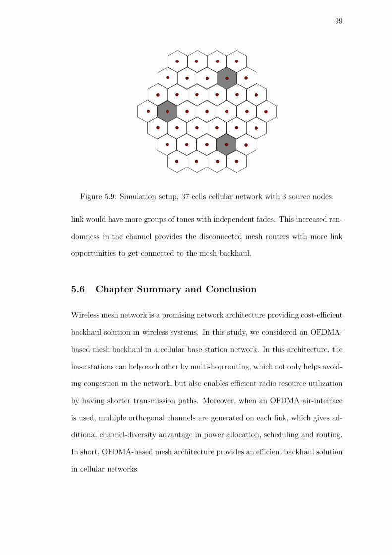
99
Figure 5.9: Simulation setup, 37 cells cellular network with 3 source nodes.
link would have more groups of tones with independent fades. This increased ran-
domness in the channel provides the disconnected mesh routers with more link
opportunities to get connected to the mesh backhaul.
5.6 Chapter Summary and Conclusion
Wireless mesh network is a promising network architecture providing cost-efficient
backhaul solution in wireless systems. In this study, we considered an OFDMA-
based mesh backhaul in a cellular base station network. In this architecture, the
base stations can help each other by multi-hop routing, which not only helps avoid-
ing congestion in the network, but also enables efficient radio resource utilization
by having shorter transmission paths. Moreover, when an OFDMA air-interface
is used, multiple orthogonal channels are generated on each link, which gives ad-
ditional channel-diversity advantage in power allocation, scheduling and routing.
In short, OFDMA-based mesh architecture provides an efficient backhaul solution
in cellular networks.
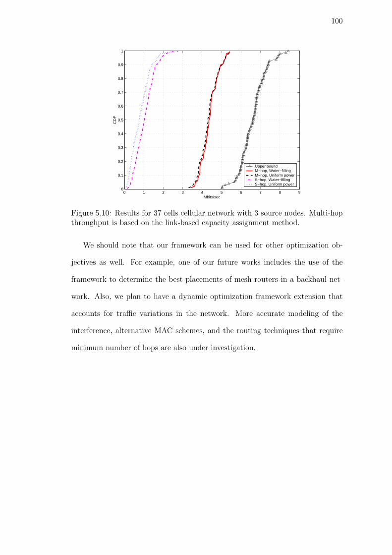
100
0 1 2 3 4 5 6 7 8 90
0.1
0.2
0.3
0.4
0.5
0.6
0.7
0.8
0.9
1
CD
F
Mbits/sec
Upper boundM−hop, Water−fillingM−hop, Uniform powerS−hop, Water−fillingS−hop, Uniform power
Figure 5.10: Results for 37 cells cellular network with 3 source nodes. Multi-hopthroughput is based on the link-based capacity assignment method.
We should note that our framework can be used for other optimization ob-
jectives as well. For example, one of our future works includes the use of the
framework to determine the best placements of mesh routers in a backhaul net-
work. Also, we plan to have a dynamic optimization framework extension that
accounts for traffic variations in the network. More accurate modeling of the
interference, alternative MAC schemes, and the routing techniques that require
minimum number of hops are also under investigation.

101
1 1.5 2 2.5 3 3.5 40
0.1
0.2
0.3
0.4
0.5
0.6
0.7
0.8
0.9
1
CD
F
Mbits/sec
Single carrierOFDMA
Figure 5.11: Single carrier vs OFDMA. 19 cells cellular network (2 rings aroundthe source node).
0 0.5 1 1.5 2 2.5 3 3.5 4 4.50
0.1
0.2
0.3
0.4
0.5
0.6
0.7
0.8
0.9
1
Mbits/sec
CD
F
Spatial water−fillingRandom link assignmentsLink−based water−filling
0.5 micros delay spread
32 micros delay spread
Figure 5.12: Spatial water-filling, random link assignments, link-based water-filling. 19 cells cellular network (2 rings around the source node). Results arepresented for 0.5µs and 32µs delay spreads.

102
Chapter 6
Conclusion
Our results indicate that the network coordination is a promising technique
suggesting large capacity improvements over the conventional cellular networks.
Without network coordination, the downlink system capacity is limited by inter-
cell interference. Furthermore, since the links often operate in the low SINR
regime, the use of multiple antennas does not improve the system capacity signif-
icantly. On the other hand, when network coordination is employed, inter-cell in-
terference is successfully eliminated. Then, the links can operate in the high SNR
regime. This enables the cellular network to enjoy the great spectral efficiency im-
provement associated with using multiple antennas. This strongly suggests that
if the multiple antennas are to be deployed in a practical interference-limited cel-
lular downlink system, it is very advisable to consider employing some form of
coordination to eliminate inter-cell interference.
The coordination requires a high-speed backbone enabling information (data,
control/syncronization and channel state) exchange between the base stations.
Moreover, the coherent methods need channel information at the base stations,
which could be achieved in practice by using channel estimates on the uplink
in the time division duplexing (TDD) mode, or by a channel feedback from the
mobiles in the frequency division duplexing mode (FDD). Also, the timing/phase
synchronization is essential to achieve coherent combining of the signals from

103
multiple base stations. Impairments due to Doppler are another challenge to be
addressed in practice. As processing power required for advanced signal process-
ing techniques improves, implementation of complex transmission techniques such
as dirty paper coding will be closer to reality.
As a future research direction, it would be interesting to have distributed, or
local, implementation of network coordination in cellular networks. To achieve
this, one has to identify essential part of the information (channel state, synchro-
nization etc.) that has to be shared among the base stations to realize significant
portion of the promised gains. For example, it might be enough for each base sta-
tion to have the channel information of a few neighboring base stations. Also, it
is important to quantify the amount of backhaul resources required to implement
network coordination in a practical system. We note that network coordination
is an example of cooperation in cellular systems, and the base stations can ac-
tually cooperate in many different ways. As an example, the base stations can
take advantage of the bursty nature of the data transmissions by sharing on-off
information to avoid interference during the bursty data arrivals. Also, spectrum
allocations can be performed in a coordinated way to avoid overlapping bursty
transmissions.
The base station coordination is a futuristic system design that may poten-
tially offer a significant capacity improvement in cellular networks. Our study
establishes the initial foundations of the design, and quantifies the theoretical
performance gains to encourage further studies striving towards these gains in
practice.

104
References
[1] G. J. Foschini and M. J. Gans, On limits of wireless communications in a fad-ing environment when using multiple antennas, Wireless Personal Commun.:Kluwer Academic Press, no. 6, pp. 311-335, 1998.
[2] E. Telatar, Capacity of multi-antenna Gaussian channels, Eur. Trans.Telecomm. ETT, vol. 10, no. 6, pp. 585-596, Nov. 1999.
[3] J.Winters, On the capacity of radio communication systems with diversityin a Rayleigh fading environment, IEEE J. Select. Areas Commun., vol. 5,pp. 871-878, June 1987.
[4] A. Goldsmith, S. Jafar, N. Jindal and S. Vishwanath, Capacity limits of theMIMO Channel, IEEE Transactions on Information Theory, Vol. 21, No. 5,June 2003, pp 684-702
[5] M. J. Gans, N. Amitay, Y. S. Yeh, H. Xu, T. Damen, R. A. Valenzuela, T.Sizer, R. Storz, D. Taylor, W. M. MacDonald, C. Tran, and A. Adamiecki,Outdoor BLAST measurement system at 2.44 GHz: Calibration and initialresults, IEEE J. Select. Areas Commun., vol. 20, pp. 570-581, Apr. 2002.
[6] G. J. Foschini, D. Chizhik, M. Gans, C. Papadias, and R. A. Valenzuela,Analysis and performance of some basic spacetime architectures, IEEE J.Select. Areas Commun., Special Issue on MIMO Systems, pt. I, vol. 21, pp.303-320, Apr. 2003.
[7] G. J. Foschini, Layered space-time architecture for wireless communicationin fading environments when using multi-element antennas, Bell Labs Tech.J., pp. 41-59, 1996.
[8] V. Tarokh, N. Seshardri, and A. R. Calderbank, Spacetime codes for highdata rate wireless communications: Performance analysis and code construc-tion, IEEE Trans. Inform. Theory, vol. 44, pp. 744-765, Mar. 1998.
[9] G. Rayleigh and J. M. Cioffi, Spatio-temporal coding for wireless channels,IEEE Trans. Commun., vol. 44, pp. 357-366, Mar. 1998.
[10] S. Alamouti, A Simple Transmitter Diversity Scheme for Wireless Commu-nication, IEEE Journal on Selected Areas in Communications, Vol. 17, No10, October 1998, pp 1451-1458.

105
[11] W. Yu, W. Rhee, S. Boyd, and J. Cioffi, Iterative Water-Filling for GaussianVector Multiple-Access Channels, IEEE Trans. Inform. Theory, vol. 50, pp145-152, Jan. 2004.
[12] R. Cheng and S. Verdu, Gaussian multiaccess channels with ISI: Capacityregion and multiuser water-filling, IEEE Trans. Inform. Theory, vol. 39, pp.773-785, May 1993.
[13] D. Tse and S. Hanly, Multiaccess fading channels-Part I: Polymatroid struc-ture, optimal resource allocation and throughput capacities, IEEE Trans.Inform. Theory, vol. 44, pp. 2796-2815, Nov. 1998.
[14] P. Viswanath, D. N. Tse, and V. Anantharam, Asymptotically optimal water-filling in vector multiple-access channels, IEEE Trans. Inform. Theory, vol.47, pp. 241-267, Jan. 2001.
[15] S. Serbetli and A. Yener, “Transceiver Optimization for Multiuser MIMOSystems”, IEEE Transactions on Signal Processing, January 2004, 52(1),pp. 214-226.
[16] Wei Yu, and John Cioffi: Sum Capacity of Gaussian Vector Broadcast Chan-nels, IEEE Transactions on Information Theory, vol. 50, no. 9, pp.1875-1892,September 2004
[17] P. Viswanath and D. N. Tse, Sum capacity of the multiple antenna Gaussianbroadcast channel, in Proc. Int. Symp. Information Theory, June 2002, p.497.
[18] S. Vishwanath, N. Jindal, and A. Goldsmith. Duality, Achievable Rates, andSum-rate Capacity of Gaussian MIMO Broadcast Channels. IEEE Transac-tions on Information Theory, 49:2658-2668, October 2003.
[19] H. Weingarten, Y. Steinberg, and S. Shamai (Shitz). The Capacity Regionof the Gaussian MIMO Broadcast Channel. In 38th Annual Conference onInformation Sciences and Systems (CISS 2004), March 17-19 2004.
[20] G. Caire and S. Shamai. On the Achievable Throughput of a MultiantennaGaussian Broadcast Channel. IEEE Transactions on Information Theory,49(7):1691-1706, July 2003.
[21] D. Samardzija, D. Chizhik and N. Mandayam, “Downlink Multiple AntennaTransmitter Optimization on Spatially and Temporally Correlated Channelswith Delayed Channel State Information”, Conf. on Info. Sciences and Sys-tems (CISS), Princeton, 2004.
[22] D. Samardzija and N. Mandayam, “Pilot Assisted Estimation of MIMO Fad-ing Channel Response and Achievable Data Rates”, IEEE Transactions onSignal Processing, Special Issue on MIMO, Vol. 51, pp. 2882-2890, November2003.
106
[23] D. Samardzija and N. Mandayam, “Unquantized and Uncoded Channel StateInformation Feedback on Wireless Channels”, Conf. on Info. Sciences andSystems (CISS), Princeton, 2004.
[24] http://www.atheros.com/pt/whitepapers/MIMO_WLAN_Perf_
whitepaper.pdf.
[25] T. M. Cover and J. A. Thomas, Elements of Information Theory. New York:Wiley, 1991.
[26] S. I. Gel’fand and M. S. Pinsker, Coding for channel with random parameters,Problems of Control and Information Theory, vol. 9, no. 1, pp. 19-31, 1980.
[27] M. Costa. Writing on Dirty Paper. IEEE Transactions on InformationTheory, 29(3):439-441, May 1983.
[28] S. Shamai and A. D. Wyner, Information-theoretic considerations for sym-metric, cellular, multiple-access fading channels, IEEE Trans. Inform. The-ory, vol. 43, pp. 1877-1991, Nov. 1997.
[29] B.M. Zaidel and S. Shamai. Enhancing the Cellular Downlink Capacity viaCo-processing at the Transmitting End. In Vehicular Technology Conference,pages 1745-1749, May 6-9 2001.
[30] S. Boyd and L. Vandenberghe. Convex Optimization. Cambridge UniversityPress, New York, NY, USA, 2004.
[31] W. Yu and T. Lan, “Transmitter Optimization for the Multi-Antenna Down-link with Per-Antenna Power Constraints”, to appear in IEEE Transactionson Signal Processing, 2006.
[32] W. Yu and T. Lan,“Downlink beamforming with per-antenna power con-straints”, Sixth IEEE International Workshop on Signal Processing Advancesin Wireless Communications (SPAWC), New York City, USA. June 2005.
[33] S. A. Vorobyov, A. B. Gershman, and Z.-Q. Luo, Robust adaptive beam-forming using worstcase performance optimization: A solution to the signalmismatch problem, IEEE Trans. Signal Process., vol. 51, no. 2, pp. 313-324,Feb. 2003.
[34] D. P. Palomar, A. Pascual-Iserte, J. M. Cioffi, and M. A. Lagunas, Con-vex Optimization Theory Applied to Joint Transmitter-Receiver Design inMIMO Channels, in Space-Time Processing for MIMO Communications,Chapter 8, pp. 269-318, John Wiley & Sons, ISBN 0-470-01002-9, April 2005.
[35] EURO-COST231, Urban Transmission Loss Models for Mobile Radio in the900 and 1800 MHz Bands: The Hague, Revision 2, Sept. 1991.

107
[36] M. Hata, Empirical Formula for Propagation Loss in Land Mobile RadioServices, IEEE Trans. Veh. Technology, Vol. VT 29, Aug. 1980
[37] G. J. Foschini and Z. Miljanic, A Simple Distributed Autonomous PowerControl Algorithm and Its Convergence, IEEE Trans. on Vehicular Tech.,Vol. 42, No. 4, Nov. 1993, pp 641-646
[38] R. Yates, A Framework for Uplink Power Control in Cellular Radio Systems,IEEE Journal on Selected Areas In Communications, Vol. 13, No. 7, Sept.1995, pp 1341-1347
[39] I. F. Akyildiz, X. Wang, and W. Wang, Wireless Mesh Networks: A Survey,Computer Networks Journal (Elsevier), vol. 47, no. 4, pp. 445-487, Mar.2005.
[40] S. Mukherjee and H. Viswanathan, Throughput Range Tradeoff of WirelessMesh Backhaul Networks, IEEE Journal on Selected Areas in Communica-tions, Vol. 24, No. 3. (2006), pp. 593-602.
[41] M. S. Kodialam and T. Nandagopal, Characterizing achievable rates in multi-hop wireless mesh networks with orthogonal channels, IEEE/ACM Trans.Netw. 13(4): 868-880 (2005).
[42] M. S. Kodialam and T. Nandagopal, Characterizing the capacity region inmulti-radio multi-channel wireless mesh networks, MOBICOM 2005: 73-87.
[43] M. Alicherry, R. Bhatia and L. Li, Joint Channel Assignment and Rout-ing for Throughput Optimization in Multi-radio Wireless Mesh Networks,Proc. ACM International Conference on Mobile Computing and Networking(MobiCom), Cologne, Germany, August 2005.
[44] R. Bhatia and M. S. Kodialam, On Power Efficient Communication overMulti-hop Wireless Networks: Joint Routing, Scheduling and Power Control,INFOCOM 2004.
[45] T. ElBatt and A. Ephremides, Joint scheduling and power control for wirelessad hoc networks, IEEE Trans. Wireless Commun., vol. 3, no. 1, pp. 74-85,Jan. 2004.
[46] R. L. Cruz and A. V. Santhanam, Optimal routing, link scheduling and powercontrol in multi-hop wireless networks, in Proc. INFOCOM, Mar./Apr. 2003,pp. 702-711.
[47] L. Xiao, M. Johansson and S. Boyd, Simultaneous routing and resource allo-cation via dualdecomposition, IEEE Transactions on Communications, vol.52, pp. 1136-1144, July 2004.
[48] R. Draves, J. Padhye, and B. Zill, Routing in Multi-radio, Multi-hop WirelessMesh Networks, ACM MobiCom, Philadelphia, PA, September 2004.

108
[49] R. Draves, J. Padhye, and B. Zill, Comparison of Routing Metrics for StaticMulti-Hop Wireless Networks, ACM SIGCOMM, Portland, OR, August2004.
[50] P. Gupta and P. R. Kumar, The Capacity of Wireless Networks, IEEE Trans-actions on Information Theory, 46(2):388-404, March 2000.
[51] S. Toumpis and A. J. Goldsmith, Capacity regions for wireless ad hoc net-works, IEEE Trans. Wireless Commun., vol. 2, no. 4, pp. 736-748, Jul. 2003.
[52] L.J. Cimini, Jr., Analysis and simulation of a digital mobile radio channelusing orthogonal frequency division multiplexing, IEEE Trans. Commun.,vol.33, no.7, pp.665-765, July 1985.
[53] K.-W. Wong, R.S.-K. Cheng, K. Ben Letaief and R.D. Murch, “Adaptiveantennas at the mobile and base stations in an OFDM/TDMA system”,IEEE Trans. Comm. 49 (1), pp.195-206, Jan. 2001.
[54] C. E. Shannon, A theorem on coloring the lines of a network, J. Math. Phys.,vol. 28, pp. 148-151, 1949.
[55] B. Hajek and G. Sasaki, Link scheduling in polynomial time, IEEE Trans.Inf. Theory, vol. 34, no. 5, pp. 910-917, Sep. 1988.
[56] T. Nishizeki and K. Kashiwagi, On the 1.1 edge-coloring of multi-graphs, inSIAM J. Discrete Math., vol. 3, no. 3, 1990, pp. 391-410.