network communities and the foreign exchange market
TRANSCRIPT

Network Communities and theForeign Exchange Market
Daniel Fenn
St. Anne’s College
University of Oxford
A thesis submitted for the degree of
Doctor of Philosophy
Trinity 2010


To my parents


Acknowledgements
I would like to thank HSBC bank and the EPSRC for funding this work.
I am grateful to Mark McDonald and Stacy Williams for helping me to
understand the intricacies of the financial data and for many useful (and
occasionally enjoyable) discussions. I would particularly like to thank Nick
Jones and Mason Porter for guiding this research and for the countless sug-
gestions and insights that have helped to shape the ideas that I present.
I would also like to thank them for comments on various manuscripts,
which encouraged me to make my explanations clearer and my arguments
more precise. I am also grateful to Sam Howison for helpful conversations
and guidance and to J.-P. Onnela for many fruitful discussions and sug-
gestions. Finally, I would like to thank Neil Johnson and Peter Mucha for
valuable input at various stages of this work.


Abstract
Many systems studied in the biological, physical, and social sciences are
composed of multiple interacting components. Often the number of com-
ponents and interactions is so large that attaining an understanding of
the system necessitates some form of simplification. A common represen-
tation that captures the key connection patterns is a network in which
the nodes correspond to system components and the edges represent in-
teractions. In this thesis we use network techniques and more traditional
clustering methods to coarse-grain systems composed of many interacting
components and to identify the most important interactions.
This thesis focuses on two main themes: the analysis of financial systems
and the study of network communities, an important mesoscopic feature
of many networks. In the first part of the thesis, we discuss some of the
issues associated with the analysis of financial data and investigate the
potential for risk-free profit in the foreign exchange market. We then use
principal component analysis (PCA) to identify common features in the
correlation structure of different financial markets. In the second part of
the thesis, we focus on network communities. We investigate the evolving
structure of foreign exchange (FX) market correlations by representing the
correlations as time-dependent networks and investigating the evolution
of network communities. We employ a node-centric approach that allows
us to track the effects of the community evolution on the functional roles
of individual nodes and uncovers major trading changes that occurred in
the market. Finally, we consider the community structure of networks
from a wide variety of different disciplines. We introduce a framework
for comparing network communities and use this technique to identify
networks with similar mesoscopic structures. Based on this similarity,
we create taxonomies of a large set of networks from different fields and
individual families of networks from the same field.


Publications
Much of the work in this thesis has been published or a manuscript has been
submitted and is under review. Details of these publications are given below.
[P1] D. J. Fenn, M. A. Porter, M. McDonald, S. Williams, N. F. John-
son, and N. S. Jones, Dynamic Communities in Multichannel Data: An
Application to the Foreign Exchange Market During the 2007-2008 Credit Cri-
sis, Chaos, 19 (2009), 033119.
[P2] D. J. Fenn, S. D. Howison, M. McDonald, S. Williams, and N. F.
Johnson, The Mirage of Triangular Arbitrage in the Spot Foreign Exchange
Market, International Journal of Theoretical and Applied Finance, 12 (2009)
pp. 1–19.
[P3] D. J. Fenn, M. A. Porter, P. J. Mucha, M. McDonald, S. Williams,
N. F. Johnson, and N. S. Jones, Dynamical Clustering of Exchange Rates,
arXiv:0905.4912, submitted (2010).
[P4] J.-P. Onnela∗, D. J. Fenn∗, S. Reid, M. A. Porter, P. J. Mucha,
M. D. Fricker, and N. S. Jones, A Taxonomy of Networks, arXiv:1006.5731,
submitted (2010).
[P5] D. J. Fenn, M. A. Porter, M. McDonald, S. Williams, N. F. John-
son, and N. S. Jones, Temporal Evolution of Financial Market Correlations,
arXiv:1011.3225, submitted (2010).
∗These authors are listed as joint first authors on these papers. I performed all of the analysisthat we describe in publication [P4] and that I present in this thesis.

I have undertaken additional research during my D. Phil. that I do not include
in this thesis due to its disparate nature. For completeness, I list the publications
resulting from this work below.
[P7] Z. Zhao, J.-P. Calderon, C. Xu, G. Zhao, D. J. Fenn, D. Sornette,
R. Crane, P.-M. Hui, and N. F. Johnson, Common group dynamic drives
modern epidemics across social, financial and biological domains, Physical Re-
view E, 81 (2010), 056107. [Selected to appear in Volume 19, Issue 11 (2010)
of the Virtual Journal of Biological Physics Research.]
[P8] D. J. Fenn, Z. Zhao, P.-M. Hui, and N. F. Johnson, Competitive carbon
emission yields the possibility of global self-control, Journal of Computational
Science, 1 (2010) pp. 63–74.
[P9] Z. Zhao, D. J. Fenn, P.-M. Hui, and N. F. Johnson, Self-organized global
control of carbon emissions, Physica A, 389 (2010) pp. 3546–3551.

Statement of Originality
The research in this thesis is a result of collaboration between myself and my coauthors
on the listed publications. My collaborators have helped develop the ideas described
in this thesis, but I have performed all of the analysis leading to the results that I
present.


Contents
1 Introduction 1
1.1 Networks . . . . . . . . . . . . . . . . . . . . . . . . . . . . . . . . . . 1
1.1.1 Topology and weighted networks . . . . . . . . . . . . . . . . 3
1.1.2 Community structure . . . . . . . . . . . . . . . . . . . . . . . 4
1.1.3 Dynamics of and on networks . . . . . . . . . . . . . . . . . . 4
1.2 Financial systems . . . . . . . . . . . . . . . . . . . . . . . . . . . . . 5
1.3 Outline . . . . . . . . . . . . . . . . . . . . . . . . . . . . . . . . . . . 6
2 Triangular Arbitrage in the FX Market 9
2.1 Introduction . . . . . . . . . . . . . . . . . . . . . . . . . . . . . . . . 9
2.1.1 The foreign exchange market . . . . . . . . . . . . . . . . . . . 10
2.1.2 Indicative versus executable prices . . . . . . . . . . . . . . . . 11
2.1.3 Prior studies . . . . . . . . . . . . . . . . . . . . . . . . . . . . 13
2.2 Triangular arbitrage . . . . . . . . . . . . . . . . . . . . . . . . . . . 14
2.3 Data . . . . . . . . . . . . . . . . . . . . . . . . . . . . . . . . . . . . 14
2.4 Arbitrage properties . . . . . . . . . . . . . . . . . . . . . . . . . . . 16
2.4.1 Rate products . . . . . . . . . . . . . . . . . . . . . . . . . . . 16
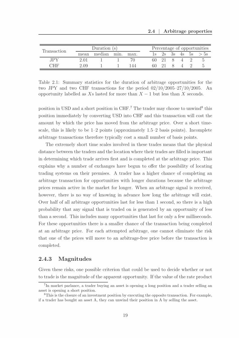
2.4.2 Durations . . . . . . . . . . . . . . . . . . . . . . . . . . . . . 17
2.4.3 Magnitudes . . . . . . . . . . . . . . . . . . . . . . . . . . . . 19
2.4.4 Seasonal variations . . . . . . . . . . . . . . . . . . . . . . . . 21
2.4.5 Annual variations . . . . . . . . . . . . . . . . . . . . . . . . . 23
2.5 Profitability . . . . . . . . . . . . . . . . . . . . . . . . . . . . . . . . 24
2.6 Fill probabilities . . . . . . . . . . . . . . . . . . . . . . . . . . . . . . 26
2.7 Summary . . . . . . . . . . . . . . . . . . . . . . . . . . . . . . . . . 30
3 Financial Market PCA 33
3.1 Introduction . . . . . . . . . . . . . . . . . . . . . . . . . . . . . . . . 33
3.1.1 Components and factors . . . . . . . . . . . . . . . . . . . . . 34
i

Contents
3.1.1.1 Factor models . . . . . . . . . . . . . . . . . . . . . . 34
3.1.1.2 Principal component and factor analysis . . . . . . . 35
3.1.2 Random matrix theory . . . . . . . . . . . . . . . . . . . . . . 37
3.2 Data . . . . . . . . . . . . . . . . . . . . . . . . . . . . . . . . . . . . 38
3.2.1 Description . . . . . . . . . . . . . . . . . . . . . . . . . . . . 38
3.2.2 Returns . . . . . . . . . . . . . . . . . . . . . . . . . . . . . . 40
3.2.3 Correlations . . . . . . . . . . . . . . . . . . . . . . . . . . . . 42
3.2.3.1 Correlations for all assets . . . . . . . . . . . . . . . 42
3.2.3.2 Intra-asset-class correlations . . . . . . . . . . . . . . 43
3.3 Principal component analysis . . . . . . . . . . . . . . . . . . . . . . 44
3.3.1 Eigenvalues . . . . . . . . . . . . . . . . . . . . . . . . . . . . 45
3.3.2 Eigenvectors . . . . . . . . . . . . . . . . . . . . . . . . . . . . 46
3.4 Temporal evolution . . . . . . . . . . . . . . . . . . . . . . . . . . . . 48
3.4.1 Proportion of variance . . . . . . . . . . . . . . . . . . . . . . 50
3.4.2 Significant principal component coefficients . . . . . . . . . . . 51
3.4.3 Number of significant components . . . . . . . . . . . . . . . . 53
3.5 Asset-component correlations . . . . . . . . . . . . . . . . . . . . . . 55
3.6 Summary . . . . . . . . . . . . . . . . . . . . . . . . . . . . . . . . . 58
4 Community Structure in Networks 61
4.1 Introduction . . . . . . . . . . . . . . . . . . . . . . . . . . . . . . . . 61
4.2 Notation . . . . . . . . . . . . . . . . . . . . . . . . . . . . . . . . . . 62
4.3 Community detection methods . . . . . . . . . . . . . . . . . . . . . . 62
4.3.1 k-clique percolation . . . . . . . . . . . . . . . . . . . . . . . . 63
4.3.2 Modularity maximization . . . . . . . . . . . . . . . . . . . . 64
4.3.3 Potts method . . . . . . . . . . . . . . . . . . . . . . . . . . . 65
4.4 Edge communities . . . . . . . . . . . . . . . . . . . . . . . . . . . . . 67
4.5 Clustering networks . . . . . . . . . . . . . . . . . . . . . . . . . . . . 67
4.6 Community dynamics . . . . . . . . . . . . . . . . . . . . . . . . . . . 68
4.6.1 Early studies . . . . . . . . . . . . . . . . . . . . . . . . . . . 69
4.6.2 Comparing and mapping communities . . . . . . . . . . . . . 71
4.6.3 Dynamics of known partitions . . . . . . . . . . . . . . . . . . 72
4.6.4 Dynamic subgraphs and cliques . . . . . . . . . . . . . . . . . 74
4.6.5 Dynamic clique percolation . . . . . . . . . . . . . . . . . . . 76
4.6.6 Edge betweenness methods . . . . . . . . . . . . . . . . . . . . 77
4.6.7 Density methods . . . . . . . . . . . . . . . . . . . . . . . . . 79
ii

Contents
4.6.8 Random walkers . . . . . . . . . . . . . . . . . . . . . . . . . 80
4.6.9 Graph colouring . . . . . . . . . . . . . . . . . . . . . . . . . . 83
4.6.10 Graph segmentation and change points . . . . . . . . . . . . . 83
4.6.11 Node-centric methods . . . . . . . . . . . . . . . . . . . . . . 85
4.6.12 Evolutionary clustering . . . . . . . . . . . . . . . . . . . . . . 88
4.6.13 Summary . . . . . . . . . . . . . . . . . . . . . . . . . . . . . 90
5 Dynamic Communities in the FX Market 93
5.1 Introduction . . . . . . . . . . . . . . . . . . . . . . . . . . . . . . . . 93
5.2 Data . . . . . . . . . . . . . . . . . . . . . . . . . . . . . . . . . . . . 94
5.2.1 Returns . . . . . . . . . . . . . . . . . . . . . . . . . . . . . . 95
5.2.2 Adjacency matrix . . . . . . . . . . . . . . . . . . . . . . . . . 96
5.3 Detecting communities . . . . . . . . . . . . . . . . . . . . . . . . . . 98
5.4 Robust community partitions . . . . . . . . . . . . . . . . . . . . . . 99
5.5 Community detection in dynamic networks . . . . . . . . . . . . . . . 102
5.5.1 Choosing a resolution . . . . . . . . . . . . . . . . . . . . . . . 102
5.5.2 Testing community significance . . . . . . . . . . . . . . . . . 103
5.5.3 Community properties . . . . . . . . . . . . . . . . . . . . . . 105
5.6 Minimum spanning trees . . . . . . . . . . . . . . . . . . . . . . . . . 107
5.7 Exchange rate centralities and community persistence . . . . . . . . . 113
5.7.1 Centrality measures . . . . . . . . . . . . . . . . . . . . . . . . 113
5.7.2 Community tracking . . . . . . . . . . . . . . . . . . . . . . . 114
5.7.3 Exchange rate roles . . . . . . . . . . . . . . . . . . . . . . . . 115
5.8 Major community changes . . . . . . . . . . . . . . . . . . . . . . . . 117
5.8.1 Mexican peso crisis . . . . . . . . . . . . . . . . . . . . . . . . 121
5.8.2 Asian currency crisis . . . . . . . . . . . . . . . . . . . . . . . 121
5.8.3 Credit crisis . . . . . . . . . . . . . . . . . . . . . . . . . . . . 121
5.9 Visualizing changes in exchange rate roles . . . . . . . . . . . . . . . 124
5.9.1 Average roles . . . . . . . . . . . . . . . . . . . . . . . . . . . 124
5.9.2 Annual roles . . . . . . . . . . . . . . . . . . . . . . . . . . . . 125
5.9.3 Quarterly roles . . . . . . . . . . . . . . . . . . . . . . . . . . 127
5.10 Robustness of results . . . . . . . . . . . . . . . . . . . . . . . . . . . 129
5.11 Summary . . . . . . . . . . . . . . . . . . . . . . . . . . . . . . . . . 130
iii

Contents
6 A Taxonomy of Networks 131
6.1 Introduction . . . . . . . . . . . . . . . . . . . . . . . . . . . . . . . . 131
6.2 Multi-resolution community detection . . . . . . . . . . . . . . . . . . 133
6.2.1 Resolution matrix . . . . . . . . . . . . . . . . . . . . . . . . . 133
6.2.2 Problems with comparing networks using resolution . . . . . . 134
6.2.3 Effective fraction of antiferromagnetic links . . . . . . . . . . . 135
6.2.3.1 Properties . . . . . . . . . . . . . . . . . . . . . . . . 136
6.3 Mesoscopic response functions . . . . . . . . . . . . . . . . . . . . . . 137
6.3.1 Example MRFs . . . . . . . . . . . . . . . . . . . . . . . . . . 139
6.3.2 MRFs for Erdos-Renyi networks . . . . . . . . . . . . . . . . . 142
6.3.2.1 Varying the fraction of possible edges . . . . . . . . . 142
6.3.2.2 Varying the number of nodes . . . . . . . . . . . . . 143
6.3.3 Synthetic MRFs . . . . . . . . . . . . . . . . . . . . . . . . . . 145
6.4 Distance measures . . . . . . . . . . . . . . . . . . . . . . . . . . . . 148
6.4.1 PCA distance . . . . . . . . . . . . . . . . . . . . . . . . . . . 149
6.4.2 Distance matrices . . . . . . . . . . . . . . . . . . . . . . . . . 150
6.5 Clustering networks . . . . . . . . . . . . . . . . . . . . . . . . . . . . 151
6.5.1 Network categories . . . . . . . . . . . . . . . . . . . . . . . . 153
6.5.2 Selecting a subset of networks . . . . . . . . . . . . . . . . . . 153
6.5.3 Choosing a linkage clustering algorithm . . . . . . . . . . . . . 155
6.5.4 Comparison of clusterings for different distances . . . . . . . . 156
6.5.4.1 Visual comparison . . . . . . . . . . . . . . . . . . . 156
6.5.4.2 Metric comparison . . . . . . . . . . . . . . . . . . . 158
6.6 Network taxonomies . . . . . . . . . . . . . . . . . . . . . . . . . . . 161
6.6.1 Taxonomy of all networks . . . . . . . . . . . . . . . . . . . . 161
6.6.2 Taxonomy of a sub-set of networks . . . . . . . . . . . . . . . 161
6.6.3 Taxonomy of network categories . . . . . . . . . . . . . . . . . 164
6.6.4 Comparison with prior clusterings . . . . . . . . . . . . . . . . 166
6.6.5 Synthetic networks . . . . . . . . . . . . . . . . . . . . . . . . 167
6.7 Clustering networks using other properties . . . . . . . . . . . . . . . 168
6.7.1 Simple network statistics . . . . . . . . . . . . . . . . . . . . . 168
6.7.2 Strength distribution . . . . . . . . . . . . . . . . . . . . . . . 170
6.8 Robustness of MRFs for different heuristics . . . . . . . . . . . . . . . 171
6.9 Case studies . . . . . . . . . . . . . . . . . . . . . . . . . . . . . . . . 172
6.9.1 U.S. Congressional roll-call voting . . . . . . . . . . . . . . . . 172
6.9.1.1 Party polarization . . . . . . . . . . . . . . . . . . . 173
iv

Contents
6.9.1.2 Using MRFs to identify periods of polarization . . . 174
6.9.1.3 Effect of polarization on the MRFs . . . . . . . . . . 178
6.9.2 United Nations General Assembly voting . . . . . . . . . . . . 178
6.9.3 Facebook . . . . . . . . . . . . . . . . . . . . . . . . . . . . . 181
6.9.4 New York Stock Exchange . . . . . . . . . . . . . . . . . . . . 183
6.9.4.1 NYSE composite index . . . . . . . . . . . . . . . . . 184
6.9.5 Foreign exchange market . . . . . . . . . . . . . . . . . . . . . 187
6.9.6 Case studies summary . . . . . . . . . . . . . . . . . . . . . . 189
6.10 Summary . . . . . . . . . . . . . . . . . . . . . . . . . . . . . . . . . 189
7 Conclusions 191
7.1 Outlook . . . . . . . . . . . . . . . . . . . . . . . . . . . . . . . . . . 193
A Details of Financial Assets 199
B Robustness of FX Communities 203
B.1 Comparison of partition energies . . . . . . . . . . . . . . . . . . . . . 203
B.2 Temporal changes in communities . . . . . . . . . . . . . . . . . . . . 203
B.3 Example community comparison . . . . . . . . . . . . . . . . . . . . . 205
B.4 Node role comparison . . . . . . . . . . . . . . . . . . . . . . . . . . . 207
C Network Details 209
D Hamiltonian and Network Details 233
D.1 Potts Hamiltonian summation . . . . . . . . . . . . . . . . . . . . . . 233
D.2 Removing self-edges . . . . . . . . . . . . . . . . . . . . . . . . . . . . 233
E Robustness of MRFs: Network Perturbations 235
E.1 Rewiring mechanisms . . . . . . . . . . . . . . . . . . . . . . . . . . . 235
E.1.1 Partial rewiring . . . . . . . . . . . . . . . . . . . . . . . . . . 236
E.1.2 Complete rewiring . . . . . . . . . . . . . . . . . . . . . . . . 236
F Robustness of MRFs: Alternative Heuristics 241
F.1 Robustness of MRFs . . . . . . . . . . . . . . . . . . . . . . . . . . . 241
F.2 Robustness of taxonomies . . . . . . . . . . . . . . . . . . . . . . . . 243
F.2.1 Dendrogram correlations . . . . . . . . . . . . . . . . . . . . . 243
F.2.2 Dendrogram randomizations . . . . . . . . . . . . . . . . . . . 244
References 247
v


List of Figures
2.1 Example exchange rate time series . . . . . . . . . . . . . . . . . . . . 15
2.2 Example rate product evolution . . . . . . . . . . . . . . . . . . . . . 16
2.3 Rate product distributions . . . . . . . . . . . . . . . . . . . . . . . . 17
2.4 Arbitrage durations distributions . . . . . . . . . . . . . . . . . . . . 18
2.5 Daily arbitrage statistics . . . . . . . . . . . . . . . . . . . . . . . . . 21
2.6 Hourly arbitrage statistics . . . . . . . . . . . . . . . . . . . . . . . . 22
2.7 Annual arbitrage statistics . . . . . . . . . . . . . . . . . . . . . . . . 24
2.8 Mean arbitrage profit/loss . . . . . . . . . . . . . . . . . . . . . . . . 26
2.9 Total arbitrage profit/loss . . . . . . . . . . . . . . . . . . . . . . . . 27
2.10 Break-even fill probabilities . . . . . . . . . . . . . . . . . . . . . . . 29
3.1 Return distribution examples . . . . . . . . . . . . . . . . . . . . . . 41
3.2 Autocorrelation functions . . . . . . . . . . . . . . . . . . . . . . . . 41
3.3 Correlation coefficients distribution . . . . . . . . . . . . . . . . . . . 43
3.4 Intra-assets-class correlations . . . . . . . . . . . . . . . . . . . . . . . 44
3.5 Eigenvalue distribution . . . . . . . . . . . . . . . . . . . . . . . . . . 47
3.6 Principal component coefficients distribution . . . . . . . . . . . . . . 49
3.7 Fraction of the variance explained by each component . . . . . . . . . 51
3.8 Participation ratio . . . . . . . . . . . . . . . . . . . . . . . . . . . . 54
3.9 Number of significant components . . . . . . . . . . . . . . . . . . . . 56
3.10 Assets-principal component correlations . . . . . . . . . . . . . . . . . 59
5.1 Effect of window length on edge weights . . . . . . . . . . . . . . . . 97
5.2 Effect of window shift on edge weights . . . . . . . . . . . . . . . . . 98
5.3 Network statistics as a function of resolution and time . . . . . . . . 101
5.4 Main plateau properties . . . . . . . . . . . . . . . . . . . . . . . . . 104
5.5 Community size and scaled energy distribution . . . . . . . . . . . . . 105
5.6 Example FX minimum spanning tree . . . . . . . . . . . . . . . . . . 110
5.7 Example FX dendrograms . . . . . . . . . . . . . . . . . . . . . . . . 112
vii
List of Figures
5.8 Community centrality statistics . . . . . . . . . . . . . . . . . . . . . 116
5.9 Community evolution: major market events . . . . . . . . . . . . . . 119
5.10 Major community changes schematic . . . . . . . . . . . . . . . . . . 120
5.11 Carry trade unwinding . . . . . . . . . . . . . . . . . . . . . . . . . . 123
5.12 Average node roles . . . . . . . . . . . . . . . . . . . . . . . . . . . . 126
5.13 Annual node roles . . . . . . . . . . . . . . . . . . . . . . . . . . . . . 127
5.14 Quarterly node roles: 1995–1998 . . . . . . . . . . . . . . . . . . . . . 128
5.15 Quarterly node roles: 2005–2008 . . . . . . . . . . . . . . . . . . . . . 129
6.1 Problems with using resolution parameter . . . . . . . . . . . . . . . 135
6.2 Cumulative resolution distribution . . . . . . . . . . . . . . . . . . . . 137
6.3 Zachary karate club fragmentation . . . . . . . . . . . . . . . . . . . 140
6.4 Example MRFs . . . . . . . . . . . . . . . . . . . . . . . . . . . . . . 141
6.5 MRFs for Erdos-Renyi networks . . . . . . . . . . . . . . . . . . . . . 143
6.6 Distribution of Λij for Erdos-Renyi networks . . . . . . . . . . . . . . 144
6.7 Synthetic MRFs . . . . . . . . . . . . . . . . . . . . . . . . . . . . . . 147
6.8 Example of the distance between mesoscopic response functions . . . 149
6.9 Distance measure correlations . . . . . . . . . . . . . . . . . . . . . . 150
6.10 Distributions of distances . . . . . . . . . . . . . . . . . . . . . . . . . 151
6.11 Block-diagonalized distance matrices . . . . . . . . . . . . . . . . . . 152
6.12 Energy dendrogram . . . . . . . . . . . . . . . . . . . . . . . . . . . . 157
6.13 Entropy dendrogram . . . . . . . . . . . . . . . . . . . . . . . . . . . 157
6.14 Number of communities dendrogram . . . . . . . . . . . . . . . . . . 158
6.15 PCA distance dendrogram . . . . . . . . . . . . . . . . . . . . . . . . 159
6.16 Metric comparison of distance measures . . . . . . . . . . . . . . . . . 160
6.17 All-network dendrogram . . . . . . . . . . . . . . . . . . . . . . . . . 162
6.18 Network category MRFs . . . . . . . . . . . . . . . . . . . . . . . . . 165
6.19 Network category taxonomy . . . . . . . . . . . . . . . . . . . . . . . 166
6.20 Dendrogram showing the positions of the synthetic networks . . . . . 168
6.21 Dendrogram showing basic network statistics . . . . . . . . . . . . . . 169
6.22 Strength distribution dendrogram . . . . . . . . . . . . . . . . . . . . 171
6.23 Metric comparison of the PCA and strength distribution distances . . 172
6.24 U.S. Congress taxonomies . . . . . . . . . . . . . . . . . . . . . . . . 175
6.25 U.S. Congress polarization . . . . . . . . . . . . . . . . . . . . . . . . 177
6.26 U.S. Congress MRFs . . . . . . . . . . . . . . . . . . . . . . . . . . . 179
6.27 Comparison of Congresses with different polarizations . . . . . . . . . 180
viii
List of Figures
6.28 U.N. General Assembly dendrogram . . . . . . . . . . . . . . . . . . . 181
6.29 Facebook dendrogram . . . . . . . . . . . . . . . . . . . . . . . . . . 182
6.30 Facebook mesoscopic response functions . . . . . . . . . . . . . . . . 183
6.31 New York Stock Exchange dendrogram . . . . . . . . . . . . . . . . . 184
6.32 New York Stock Exchange composite index . . . . . . . . . . . . . . . 186
6.33 New York Stock Exchange volatility . . . . . . . . . . . . . . . . . . . 186
6.34 Foreign exchange market dendrogram . . . . . . . . . . . . . . . . . . 188
B.1 Distribution of energies for different heuristics . . . . . . . . . . . . . 204
B.2 Comparison of greedy and simulated annealing partitions . . . . . . . 205
B.3 Heuristic comparison: community change schematic . . . . . . . . . . 206
B.4 Heuristic comparison: quarterly node roles . . . . . . . . . . . . . . . 208
D.1 The problem with summing over all i, j in the Potts Hamiltonian . . 234
E.1 Distance matrices for partially rewired networks . . . . . . . . . . . . 237
E.2 Distribution of the number of edge rewirings . . . . . . . . . . . . . . 239
E.3 Distance matrices for completely rewired networks . . . . . . . . . . . 240
F.1 MRF comparison for different heuristics . . . . . . . . . . . . . . . . 242
F.2 Dendrogram comparison for different heuristics . . . . . . . . . . . . 243
F.3 Ultrametric correlation coefficient distributions . . . . . . . . . . . . . 246
ix


List of Tables
2.1 Arbitrage duration statistics . . . . . . . . . . . . . . . . . . . . . . . 19
2.2 Arbitrage magnitude statistics . . . . . . . . . . . . . . . . . . . . . . 20
2.3 Hours of market liquidity . . . . . . . . . . . . . . . . . . . . . . . . . 22
2.4 Annual arbitrage statistics . . . . . . . . . . . . . . . . . . . . . . . . 23
5.1 Examples of frequently observed communities . . . . . . . . . . . . . 108
5.2 Exchange rates with high centralities . . . . . . . . . . . . . . . . . . 118
6.1 Network categories . . . . . . . . . . . . . . . . . . . . . . . . . . . . 154
A.1 Details of financial assets . . . . . . . . . . . . . . . . . . . . . . . . . 199
C.1 Network details . . . . . . . . . . . . . . . . . . . . . . . . . . . . . . 212
xi


Chapter 1
Introduction
1.1 Networks
A variety of systems studied across a range of academic disciplines are composed of
multiple components that interact with each other in some way. Often these systems
are described as complex [47]. Although there is no precise definition of a complex
system, roughly speaking, a system is considered complex if it possesses many parts,
whose behaviours are highly variable and strongly dependent on the behaviours of
the other parts [270,274]. Many authors also agree that for a system to be considered
complex, it should possess emergent properties that arise through the interactions of
the components in the absence of any central controller [13]. However, the concept of
emergence is also slippery and there is currently no standard definition [25, 51, 172].
Irrespective of the precise definitions of complex systems and emergence, for systems
composed of interacting components, the pattern of connections between the com-
ponents are often crucial to the behaviour of the system. The system cannot be
understood by studying the parts in isolation; it is essential to consider the interac-
tions.
When studying systems that possess many components and interactions, to make
the analysis tractable it is often necessary to simplify the analysis by focusing on a
subset of key interactions. A common way of studying the pattern of interactions
in a given system is to construct a network (or graph) in which the components
are represented as nodes and the connections are represented as edges [9, 60, 217,
223].1 A network is therefore a simplified representation that reduces a system to a
structure that captures only the key connection patterns; however, information is lost
in the simplification process, so for any analysis to be meaningful it is important to
1Nodes are sometimes referred to as vertices and edges as links. In this thesis, we use these termsinterchangeably.
1

Chapter 1 | Introduction
ensure that the discarded details are not critical to the properties of the system being
investigated. Networks can take different forms: they can be embedded in Euclidean
space, such as airline networks and neural networks; or they can be defined in an
abstract space, such as social networks2 and language networks [46].
Traditionally, the study of networks lay within the domain of graph theory [49],
which is usually considered to date back to 1736 when Euler published a solution to
the Konigsberg bridge problem. Initially graph theory focused on regular graphs, but
since the 1950s graph theorists have also investigated random graphs [50]. This shift
was stimulated by the work of Rapoport [249,250,277] and Erdos and Renyi [86–88] on
a simple random graph model. In the model, one begins with N nodes and connects
them uniformly at random with probability p, creating a graph which on average has12pN(N − 1) edges distributed at random.
In addition to the developments in mathematical graph theory, beginning in the
1920s, social scientists started to use networks to study the relationships between
social entities, e.g., [76, 98, 111, 213, 249, 251, 258, 304]. Because of the difficulty in
collecting and analyzing large data sets, most of the early studies of social networks
were very small and the networks usually only included tens of nodes. In many of these
studies, the social scientists were often interested in answering questions relating to
the meaning of edges in the networks, such as whether they arose through friendship,
obligation, strategic alliance, or something else [127].
In the late 1990s, a surge of interest in network research across a wide range of
disciplines [225] was sparked by the publication of seminal papers by Watts and Stro-
gatz [305] and Barabasi and Albert (BA) [26]. These and subsequent developments
in network science were made possible by two key factors: (1) the computerization of
data acquisition, which meant that it was significantly easier to collect data for large
networks, and (2) the increase in computational resources, which enabled researchers
to analyze these data sets. An important observation from the new data was that,
in contrast to ER random graphs, real-world networks often possess significant inho-
mogeneities.3 For example, many networks display the “small-world” phenomenon –
despite the fact that networks contain a large number of nodes, there is often a rela-
tively short path between two nodes (i.e., a small average path length) – studied by
Milgram [209], whose work spawned the phrase the six degrees of separation. Watts
and Strogatz observed that networks that possess the small-world property often also
2Social networks can sometimes contain implicit geographical information.3An example of a homogeneous property of ER random graphs is the degree (number of neigh-
bours) of each vertex. Because there is an equal probability of all edges existing, most nodes in ERnetworks have similar degrees.
2

1.1 | Networks
show high levels of clustering – two nodes with a common neighbour are more likely
to be connected [305]. Another important observation was that the degree distribu-
tion of many real-world networks significantly deviates from the Poisson distribution
expected for random graphs, with some nodes having significantly more edges than
expected. This led Barabasi and Albert (BA) [26] to propose a preferential attach-
ment model for network growth (in which there is a higher probability for new edges
to attach to nodes with high degree) which produces network with a power-law degree
distribution.4
1.1.1 Topology and weighted networks
Much of the early work on networks focused on topological properties and the char-
acterization of unweighted networks. In unweighted networks, two nodes are either
connected or they are not; all edges in the network have the same weight. Many
features of a network depend on its topology. For example, topology is crucial to
the robustness of a network to external perturbations such as random failures or
targeted attacks on nodes [10, 46, 56, 62, 70, 151]. Topology also plays an important
role in the behaviour of different spreading processes operating on the network, such
as the spread of diseases, information, or rumours [46, 191, 213, 236, 316]. In many
networks there are also heterogeneities in the capacity or intensity of the edges [232].
The heterogeneities in the interaction strengths between components has important
effects on the function and behaviours of many systems, which has led to the study
of networks in which a weight (usually a real number) is associated with each edge.
For example, a consideration of weighted networks [232] has provided insights into
Granovetter’s weak ties hypothesis [135], which states that the relative overlap of the
friendship circles of two individuals increases with the strength of the links connect-
ing them. Another network in which connection weights play an important role is
the internet. The internet is a network for transmitting data; in its simplest network
representation, the nodes correspond to computers and other devices and the edges
represent physical connections between them, such as optical fibre lines [223]. These
connections have different bandwidths and different amounts of data flowing down
them at any point in time. Because of these heterogeneities, it is necessary to consider
link weight in order to determine optimal paths for routing data around the internet.
4In fact, this type of “rich get richer” growth mechanism dates back to the works of Yule [314],Simon [273], and Price [246].
3

Chapter 1 | Introduction
1.1.2 Community structure
A further inhomogeneity in the structure of real-world networks is in the local distri-
bution of edges. In many networks, there are high concentrations of edges between
particular groups of vertices, with relatively fewer edges between different groups.
This feature of networks is termed community structure [105,244]. Although there is
no rigorous definition, a “community” is usually considered to be a group of nodes that
are relatively densely connected to each other but sparsely connected to other dense
groups in the network. Network comunities can represent functionally-important sub-
networks [2,75,105,107,121,139,243,244,295] and their identification can have useful
applications. For example, identifying groups of customers with similar interests in
networks representing the relationships between customers and products that they
purchase can lead to the development of improved product recommendation systems
for on-line retailers [253]. The algorithmic detection of communities and the devel-
opment of tools to analyze them is currently one of the most active areas of research
in networks [105,244]. We return to communities in Chapter 4 in which we present a
more detailed discussion of the different community detection methods.
1.1.3 Dynamics of and on networks
Another active area of research is the study of the dynamical behaviour of networks,
both in terms of the structural dynamics of the networks themselves, e.g., [23,185,233]
and the dynamics of processes taking place on the network, e.g., [10,46,56,62,70,123,
151]. Most early studies of networks involved the analysis of a network at a fixed
point in time or the analysis in a single network of all of the cumulative interactions
up to a point in time, e.g., [127]. An example of the latter is the construction of
coauthorship networks that represent all collaborations between researchers during
a time period [216]. Many different approaches have been adopted for constructing
and analyzing the structural dynamics of networks. For example, networks have
been constructed in which the interactions accumulate over time and the network
dynamics investigated by comparing the structure of the aggregate network with its
structure at earlier points in time, e.g., [152]. A related approach is to construct
cumulative networks, but to add an additional decay parameter that reduces the
weight of edges based on the time that had elapsed since the interaction took place
and to remove edges whose weight falls below a threshold. The network dynamics can
then be investigated by observing changes taking place in the network, e.g., [233]. A
4
1.2 | Financial systems
third possibility is the comparison of networks for interactions aggregated over non-
overlapping time windows, e.g., [92].
The spreading processes on network (such as the spread of diseases, information,
or rumours) mentioned earlier in this section in the context of network topology are
particular examples of the more general concept of dynamical systems on networks
[223]. A dynamical system is any system whose state, as represented by some set of
variables, changes over time according to a set of rules or equations [281]. Typically,
dynamical systems on networks consist of independent dynamical variables associated
with each node that are only coupled together along the edges of the network. Many
real-world processes can be represented as dynamical systems operating on a network.
For example, the flow of traffic on roads, electricity over power grids, or the changing
concentrations of metabolites in cells [223]. One particular area of focus is the study of
the synchronization of coupled oscillators on networks, which represents an important
feature of many real-world systems [15,46]. For example, evidence suggests that there
is a pathological synchronization of neural populations during epileptic attacks [46].
In this thesis, we investigate the properties of networks possessing each of the
characteristics described in the previous three sections. In Chapter 5, we analyze
the evolving community structure of a dynamic, weighted network, and in Chapter 6
we compare the community structures of a wide variety of weighted and unweighted
networks.
1.2 Financial systems
In Chapters 2, 3, and 5, we focus on financial markets, which are often considered
to be evolving complex systems [14, 18, 19, 45]. Markets are composed of a myriad
of financial agents, such as banks, consumers, investors, and companies, that con-
tinually adjust their buying and selling decisions, prices and forecasts based on the
state of the market, which is itself determined by these decisions [18]. The state
of the market emerges through this system of interactions and feedback and cannot
be determined by considering the individual components in isolation. Because of
the wealth of components and the complex pattern of connections between them, to
gain any insights into financial systems it is necessary to focus on particular subsets
of components and interactions. For example, insights into to the global economy
can be attained by studying the flow of imports and exports between different coun-
tries [275]. However, even focusing on a particular aspect of the financial system,
the number of interactions is often so large that further simplification is required.
5

Chapter 1 | Introduction
Several studies have attempted to tackle this problem using networks. For example,
networks have been used to analyze the trade relationships between nations [275] and
liabilities in the inter-bank lending market [52]. Perhaps the most common applica-
tion of networks to financial market is in the study of the relationships between the
price time series of financial assets, e.g., [197,198,229]. In this approach, each node in
the network represents an asset and each weighted edge represents a time-dependent
correlation between the asset price time series.
In Chapter 5, we study FX market networks in which each node represents an
exchange rate and the edges represent the correlations between rates. An argument
made to justify the study of networks constructed from asset price time series is as
follows [228]. In markets, traders repeatedly compete for a limited resource, as they
buy and sell assets, with the exact timing of these trading decisions often driven by
exogenous events, such as news announcements, scheduled economic data releases,
and other events. Although the exact nature of the interactions between market
participants is often not known, the asset prices should reflect the complex pattern of
actions, feedback, and adaptation of traders, so the price time series can be considered
as the manifestation of these interactions. Under these assumptions, instead of the
nodes representing the interacting components (i.e., the traders), they represent the
resource that the components are competing for (i.e., the assets) and instead of the
edges representing the interactions between the components (i.e., buying and selling
actions) they represent correlations in a signal that results from this process (i.e., the
asset price).
Irrespective of the exact relationship between the network and the underlying
financial system, it is insightful to investigate networks based on the correlations
between different assets. In fact, this example demonstrates the power of the network
framework. Because we work with networks in an abstract form, the tools of network
analysis can in theory be applied to any system that can be represented as a network
[223]. In essence, networks methods are simply a set of techniques for studying and
identifying patterns in data generated by interacting systems. Of course, the insights
that can be gained using a network approach depend on the suitability of the technique
to the problem and for some systems other methods will be more appropriate.
1.3 Outline
This thesis is organized into six additional chapters. In each chapter in which we
present new research we provide an overview of the relevant literature and a motiva-
6

1.3 | Outline
tion for the work. The chapters are more or less distinct and can be read in isolation.
However, a continuous thread runs through the thesis as we move from an analysis of
financial systems to an investigation of communities in financial systems to a study
of communities in systems from a wide variety of different disciplines.
In Chapter 2, we discuss some of the problems associated with analyzing financial
data and present a study in which the type of data used is critical to the output of the
analysis. We also describe the FX market, which is the focus of Chapters 2 and 5. The
results of Chapter 2 answer a question of particular interest to market practitioners
regarding the possibility of making risk-free profit in the FX market. In Chapter 5, we
continue to investigate financial markets, but we extend the analysis to include assets
from a variety of different markets. We study the correlation structure across these
different markets by using principal component analysis to coarse-grain the data and
identify common features. We then study the way in which these relationships evolve
through time and discuss how the features are affected by different market events.
In the remainder of the thesis, we focus on communities in networks. In Chapter 4
we describe some of the most widely used techniques for detecting communities in
networks and present a relatively comprehensive review of the literature on communi-
ties in dynamic networks. In Chapter 5, we study the structure of the FX market by
representing the correlations between currency exchange rates as time-dependent net-
works and investigating the evolution of network communities. We propose a method
for tracking communities in dynamical networks and use this approach to identify
significant changes in the structure of the FX market. In Chapter 6, we investigate
the community structure of networks from a range of different disciplines, including
biology, sociology, politics, and finance, and introduce a framework for comparing
network communities. We use this technique to identify networks with similar meso-
scopic structures. Based on this similarity, we create taxonomies of a large set of
networks from different fields and individual families of networks from the same field.
Finally, in Chapter 7, we offer some conclusions and suggest some possible directions
for future research.
7


Chapter 2
The Mirage of TriangularArbitrage in the Foreign ExchangeMarket
The work described in this chapter has been published in reference [P2]. We highlight
that this is an empirical chapter and the analysis we present is not technical. However,
this simplicity serves to emphasize one of the main purposes of this chapter which is
to demonstrate that one needs to exercise caution when analyzing financial data. If
one uses data that is inappropriate for a particular analysis, it is easy to reach false
conclusions. We show how even for the simplest financial questions, seemingly similar
data can produce very different results. In demonstrating this, we answer a question
of interest to financial market practitioners.
2.1 Introduction
The advance in computing power during the last two decades has facilitated the stor-
age and analysis of increasingly large data sets. The increased storage capacity is
particularly useful in financial markets because, as well as enabling market partici-
pants to record details of executed transactions, institutions are now able to record
additional market information even if a trade is not executed (such as the best avail-
able price and the volume available at this price). The increased computing power has
also enabled exchanges to publish prices at increasingly higher frequencies, with some
exchanges in the FX market now publishing price updates every 250 milliseconds.
The availability of these enormous, accurate, high-frequency data sets has pro-
vided economists and financial mathematicians with unprecedented resources to test
their models and has resulted in many researchers from other disciplines studying fi-
9

Chapter 2 | Triangular Arbitrage in the FX Market
nancial problems. However, the widespread availability of this data is a double-edged
sword: while it is undoubtedly positive that more financial data is widely accessible,
this has also led to work in which data is used that is not appropriate for the study.
Asset prices provide a good example of where confusion can arise because single
assets can have several prices associated with them. For example, assets can have
an indicative price (a quote providing an indication of the level at which an asset is
currently trading), an executable price (the price at which a trade can actually be
executed in the market at a particular time, although the party posting the price
can remove it before an opposite trade is matched against it), or a traded price (the
price at which a trade is actually executed). The most appropriate price for a study
depends on the question being posed. Financial time series can also have specific
peculiarities associated with them. For example, many currencies are pegged to the
U.S. dollar, which results in their exchange rates tracking the U.S. dollar exchange
rate. If one does not use the correct type of data, or fails to deal properly with
asset-specific artifacts, then the wrong conclusions can easily be reached.
In this chapter, we investigate triangular arbitrage within the spot FX market1
using high-frequency executable prices [73]. Arbitrage is the practice of taking advan-
tage of mis-pricings in financial markets to realize risk-free profits; triangular arbitrage
is the simplest arbitrage in the FX market. As an example of triangular arbitrage,
consider the situation where one initially holds xi euros. If one sells these euros and
buys dollars, converts these dollars into Swiss francs, and then converts these francs
into xf euros, if xf > xi a profit is realized. This is a triangular arbitrage.
Prior studies of triangular arbitrage indicate the existence of large arbitrage op-
portunities that remain in the market for long periods of time, e.g., [7,169]; however,
such profit opportunities would come as something of a surprise to most FX traders.
We demonstrate that the incorrect identification of triangular arbitrage opportunities
in these prior studies results from the use of the wrong type of data. Although the
original objective of this study was to determine whether or not triangular arbitrage
opportunities exist, the study serves as a good example of the care that one needs to
take when analyzing financial data.
2.1.1 The foreign exchange market
The FX market is the world’s largest financial market with an average daily trade
volume of approximately 3.2 trillion U.S. dollars [147]. Prices in the FX market
1In the spot FX market, currencies are bought and sold for immediate delivery (actually twobusiness days after the trade day), rather than for delivery in the future.
10

2.1 | Introduction
are quoted as exchange rates of the form XXX/YYY, which indicate the amount of
currency YYY that one would receive in exchange for one unit of currency XXX. In
this thesis, we refer to currencies with the standard three letter abbreviations (tickers)
used to identify them in the FX market. The codes for the currencies we study are
USD - U.S. dollar, CHF - Swiss franc, JPY - Japanese yen, EUR - euro, DEM -
German mark, AUD - Australian dollar, CAD - Canadian dollar, XAU- gold2, GBP
- pounds sterling, NZD - New Zealand dollar, NOK - Norwegian krone, and SEK -
Swedish krona. In contrast to most other markets, the FX market is liquid 24 hours
a day.3 There are two prices quoted for an exchange rate: a bid and an ask price.
These give the different prices at which one can buy and sell currency, respectively,
with the ask price tending to be larger than the bid price. The exchange rate between
EUR and USD may, for example, be quoted as 1.4085/1.4086. A trader then looking
to convert USD into EUR might have to pay 1.4086 USD for each EUR, while a
trader looking to convert EUR to USD may receive only 1.4085 USD per EUR. The
difference between the bid and ask prices is the bid-ask spread.
2.1.2 Indicative versus executable prices
Although prior studies of triangular arbitrage exist, e.g., [7, 169], there is no robust
study that provides a definitive answer to the question of whether triangular arbitrage
can be profitable. The main reason for this is that, until recently, the available data
has not been sufficiently accurate or of a sufficiently high frequency.
As a result of the size and liquidity of the FX market, price updates occur at
extremely high frequencies. For example, the EUR/USD rate has in excess of 100 price
updates a minute during the most liquid periods. Therefore one requires an equally
high-frequency data set to test for triangular arbitrage opportunities. In addition, it is
necessary to know that the prices are ones at which a trade could indeed be executed
as opposed to simply being indicative price quotes. An indicative bid/ask price is a
quote that gives an approximate price at which a trade can be executed; at a given
time one may be able to trade at exactly this price or, as is often the case, the real price
at which one executes the trade, the executable price, differs from the indicative price
2We include gold in the study because it has many similarities with a currency [204].3There are many different definitions of liquidity [263]. We consider the market to have high
liquidity if there is a large depth of resting orders and this depth is refreshed quickly when ordersare filled. A resting order is an order to buy at a price below or sell at a price above the prevailingmarket price. Such orders are not filled immediately, but instead rest on the order book until theyare matched. High liquidity implies that one can usually find a counterparty to a trade.
11

Chapter 2 | Triangular Arbitrage in the FX Market
by a few basis points4. The main purpose of an indicative price is to supply clients of
banks with a gauge of where the price is. A large body of academic research into the
FX market has been performed using indicative quotes often under the assumption
that, due to reputational considerations, “serious financial institutions” are likely to
trade at exactly the quoted price, especially if they are hit a short time after the
quote is posted [73, 74, 138]. The efficiency of using indicative quote data for certain
analyses has, however, been drawn into question, e.g., [193,200]. In Ref. [193], Lyons
highlights some of the key problems with indicative prices: indicative prices are not
transactable; the indicative bid-ask spread, despite usually “bracketing” the actual
tradeable spread, is usually two to three times as large (i.e., the tradeable bid and
ask prices usually lie between the indicative bid and ask prices); during periods of
high trading intensity market makers are too busy to update their indicative quotes;
and market makers themselves are unlikely to garner much of their high-frequency
information from indicative prices. In the FX market today indicative prices are
typically updated by automated systems, nevertheless the quoted price is still not
necessarily a price at which one could actually execute a trade.
Goodhart et al. [131] performed a comparison of indicative bid-ask quotes from
the Reuters FXFX page and executable prices from the Reuters D2000–2 electronic
broking system over a 7 hour period and found that the behaviour of the bid-ask
spread and the frequency at which quotes arrived were quite different for the two
types of quote. In particular, the spread from the D2000–2 system showed greater
temporal variation, with the variation dependent upon the trading frequency. In
contrast, the indicative price spread tended to cluster at round numbers, a likely
artifact of the use of indicative prices as a market gauge. This discrepancy between
indicative and executable prices is likely to be less important if one is performing a
low frequency study, arguably down to time scales of 10–15 minutes [138]. If, however,
one is considering very high-frequency data, this difference becomes highly significant.
For example, in Ref. [130] Goodhart and Figliuoli find a negative first-order auto-
correlation in price changes at minute-by-minute frequencies using indicative data.
In Ref. [131], however, Goodhart finds no such negative auto-correlation when real
transaction data is used. Indicative data seem particularly unsuitable to many market
analyses today because banks are now able to provide their clients with automated
4A basis point is equal to 1/100th of a percentage point. In this paper we will also discuss points,where a point is the smallest price increment for an exchange rate. For example, for the EUR/JPYexchange rate, which takes prices of the order of 139.60 over the studied period, 1 point correspondsto 0.01. In contrast, for the EUR/USD rate with typical values around 1.2065, 1 point correspondsto 0.0001.
12

2.1 | Introduction
executable prices through an electronic trading platform so there is even less incentive
for them to make their indicative quotes accurate.
2.1.3 Prior studies
Some analyses of triangular arbitrage have been undertaken using indicative data. In
Ref. [7], Aiba et al. investigated triangular arbitrage using indicative quote data pro-
vided by information companies for the set of exchange rates EUR/USD, USD/JPY,
EUR/JPY over a roughly eight week period in 1999. They found that, over the
studied period, arbitrage opportunities appeared to exist about 6.4% of the time,
or around 90 minutes each day, with individual arbitrages lasting for up to approxi-
mately 1, 000 seconds. In Ref. [169], Kollias and Metaxas investigated 24 triangular
arbitrage relationships, using quote data for seven major currencies over a one month
period in 1998, and found that single arbitrages existed for some currency groups for
over two hours, with a median duration of 14 and 12 seconds for the two transactions
formed from USD/DEM, USD/JPY, DEM/JPY.When considering whether triangular arbitrage transactions can be profitable it
is important to consider how long the opportunities persist. The time delay between
identifying an opportunity and the arbitrage transaction being completed is instru-
mental in determining whether a transaction results in a profit because the price may
move during this time interval. Kollias and Metaxas [169] tested the profitability of
triangular arbitrage transactions by considering execution delays of between 0 and
120 seconds and, in a similar manner, Aiba et al. accounted for delays by assuming
that it took an arbitrageur between 0 and 9 seconds to recognize and execute an
arbitrage transaction. Kollias and Metaxas found that for some transactions triangu-
lar arbitrage continued to be profitable for delays of 120 seconds and Aiba et al. for
execution delays of up to 4 seconds. These durations differ markedly from the beliefs
of market participants; we suggest that this discrepancy results from the invalid use
of indicative data in these studies.
In contrast to prior studies, in this chapter we use high-frequency, executable price
data to investigate triangular arbitrage. This means that, for each arbitrage oppor-
tunity that we identify, one could potentially have executed a trade at the arbitrage
price. Furthermore, and importantly, we consider the issue of not completing an ar-
bitrage transaction. In the FX market today, where electronic trading systems are
widely used, it is possible to undertake the three constituent trades of an arbitrage
transaction in a small number of milliseconds; but, despite this execution speed, one
13

Chapter 2 | Triangular Arbitrage in the FX Market
is not guaranteed to complete a triangular arbitrage transaction. We discuss the
reasons for this in Section 2.4.2.
2.2 Triangular arbitrage
In a market as liquid as the FX market, one would expect triangular arbitrage op-
portunities to be limited and, if they do occur, for the potential profits to be small.
This means that when identifying arbitrage opportunities on a second-by-second time
scale the possible discrepancy between an indicative and an executable price becomes
extremely important. It is, in fact, essential to use executable data if one is to draw
reliable conclusions on whether triangular arbitrage opportunities exist.
Triangular arbitrage opportunities can be identified through the rate product
γ(t) =
3∏
i=1
pi(t), (2.1)
where pi(t) denotes an exchange rate at time t [7]. An arbitrage is theoretically
possible if γ > 1, but a profit will only be realized if the transaction is completed at
an arbitrage price.
For each group of exchange rates there are two unique rate products that can be
calculated. For example, consider the set of rates EUR/USD, USD/CHF, EUR/CHF.If one initially holds euros, one possible arbitrage transaction is EUR→USD→CHF→EUR
with a rate product given by
γ1(t) =
[
EUR/USDbid(t)
]
×[
USD/CHFbid(t)
]
×[
1
EUR/CHFask(t)
]
; (2.2)
the second possible arbitrage transaction is EUR→CHF→USD→EUR with a rate
product
γ2(t) =
[
1
EUR/USDask(t)
]
×[
1
USD/CHFask(t)
]
×[
EUR/CHFbid(t)
]
. (2.3)
These two rate products define all possible arbitrage transactions using this set of
exchange rates.
2.3 Data
The data we use for the analysis consists of second-by-second executable prices for
EUR/USD, USD/CHF, EUR/CHF, EUR/JPY, USD/JPY. We investigate trian-
gular arbitrage opportunities for the transactions involving EUR/USD, USD/CHF,
14

2.3 | Data
EUR/CHF and EUR/USD, USD/JPY, EUR/JPY for all week days over the pe-
riod 02/10/2005–27/10/2005 and we compare the results with those for two earlier
periods: 27/10/2003–31/10/2003 and 01/10/2004–05/10/2004.5 The full data set
consists of approximately 2.6 million data points for each of the rate products γ1 and
γ2, 5.2 million data points for each of the currency groups, and 10.4 million data
points in total. A rate product, indicating whether or not a triangular arbitrage op-
portunity existed, was found for each of these points. We show a sample of one of the
sets of exchange rates and the corresponding time series of bid-ask spreads in Fig.
2.1.
00:00 06:00 12:00 18:00 24:001.1950
1.2000
1.2050
pric
e
EUR/USD
00:00 06:00 12:00 18:00 24:001.2800
1.2850
1.2900
1.2950
time
USD/CHF
00:00 06:00 12:00 18:00 24:001.5460
1.5470
1.5480
1.5490EUR/CHF
bidask
00:00 06:00 12:00 18:00 24:00
0
2
4
6
spre
ad
00:00 06:00 12:00 18:00 24:00
0
2
4
6
8
10
time00:00 06:00 12:00 18:00 24:00
0
2
4
6
8
10
Figure 2.1: Exchange rate time series for EUR/USD, USD/CHF and EUR/CHFon 12/10/2005. Upper: bid and ask prices. Lower: bid-ask spread. Each markerrepresents the spread at a single time step. The vertical axes have been truncated tomake the detail around the typical values clearer.
5All times in this paper are given in GMT. The full day 28/10/2005 is excluded from the analysisfor the JPY group of exchange rates due to an error with the data feed on this day. During periodsof lower liquidity it is possible that there were times at which no party was offering a bid and/or askprice. At these times it would not have been possible to complete a triangular transaction involvingthe missing exchange rate so we set the associated rate product to zero.
15

Chapter 2 | Triangular Arbitrage in the FX Market
2.4 Arbitrage properties
2.4.1 Rate products
Figure 2.2 shows an example of the temporal evolution of the rate product γ over one
of the weeks analyzed. If it were possible to buy and sell a currency at exactly the
same price then one would expect the rate product to always equal one. However, the
prices at which currencies can be bought and sold differ, with the ask price exceeding
the bid price, and as a result the rate product is typically expected to be slightly less
than one. Rate products with a value just below one can be considered to fall in a
region of “triangular parity”.6
03/10/05 04/10/05 05/10/05 06/10/05 07/10/050.9980
0.9988
0.9996
1.0004
time
γ
03/10/05 04/10/05 05/10/05 06/10/05 07/10/051.0000
1.0002
1.0004
time
γ
Figure 2.2: Rate product evolution for the period 03/10/2005–07/10/2005 for thetransaction EUR→USD→JPY→EUR. Upper: all rate products, with a few extremevalues removed so that the structure around the typical values is clearer. All pointsabove the red line correspond to potential triangular arbitrages. Lower: the same plottruncated vertically at γ = 1 so that each spike represents an arbitrage opportunity.
The distributions in Fig. 2.3 show that, as expected, the rate product tends to be
slightly less than one and typically γ ∈ [0.9999, 1]. The log-linear plots also highlight
that the distributions possess long tails extending to smaller values of the rate product
and that there are some times when γ > 1. This means that for the majority of
6Triangular parity implies that the direct exchange rate is equal to the exchange rate generatedthrough the cross-rates. For example, EUR/USD = (EUR/JPY)/(USD/JPY), where one needs touse the correct bid and ask price to construct the synthetic exchange rate.
16

2.4 | Arbitrage properties
deviations from triangular parity the individual exchange rates are shifted in such
a direction that triangular arbitrage is not possible, but that occasionally potential
profit opportunities do occur. Over the four week period analyzed there are 10, 018
triangular arbitrage opportunities for the two CHF-based transactions given by Eqs.
(2.2) and (2.3) and 11, 367 for the equivalent JPY transactions.
We now establish both the duration and magnitude of these potential arbitrages
and attempt to determine whether or not they represent genuine, executable profit
opportunities.
0.994 0.996 0.998 1.0000
1
2
3
4
5x 10
5 JPY
γ
freq
uenc
y
0.994 0.996 0.998 1.00010
0
102
104
γ
freq
uenc
y
0.994 0.996 0.998 1.0000
1
2
3
4
5x 10
5
γ
freq
uenc
y
CHF
0.994 0.996 0.998 1.00010
0
102
104
γ
freq
uenc
y
Figure 2.3: Occurrence frequency for rate products of different magnitudes for theperiod 02/10/2005–27/10/2005. Upper: aggregated results for both JPY transactionsand CHF transactions. Any parts of the histograms to the right of the line at γ = 1correspond to potential triangular arbitrages. The JPY panels show all data pointswithin this period and the CHF panels all points except a few at very small and verylarge γ. Lower: the same distributions on a log-linear scale.
2.4.2 Durations
Firstly, we consider the length of periods for which γ > 1 and thus over which trian-
gular arbitrage opportunities exist. We define an X second arbitrage as one for which
γ > 1 for more than X − 1 seconds, but less than X consecutive seconds. In Fig. 2.4,
we show the distributions of the observed durations of arbitrage opportunities and
we provide summary statistics for these distributions in Table 2.1. The vast majority
of arbitrage opportunities are very short in duration; although some opportunities
17
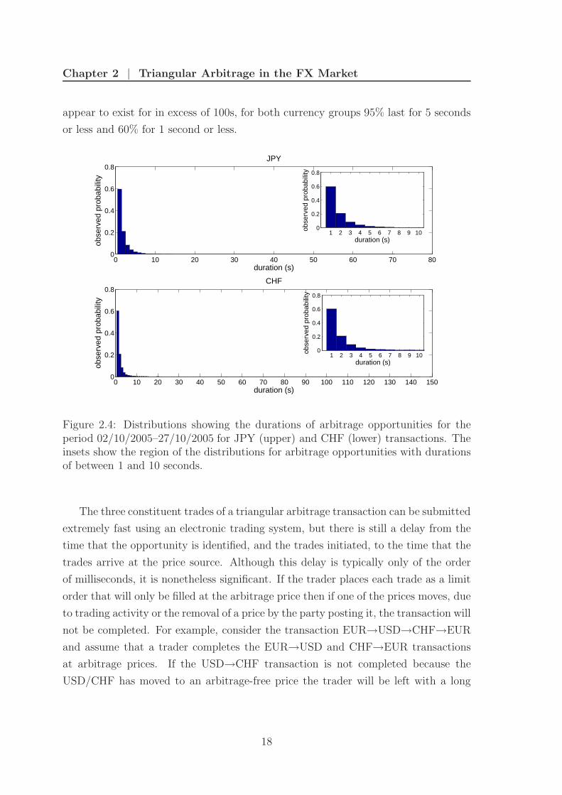
Chapter 2 | Triangular Arbitrage in the FX Market
appear to exist for in excess of 100s, for both currency groups 95% last for 5 seconds
or less and 60% for 1 second or less.
0 10 20 30 40 50 60 70 800
0.2
0.4
0.6
0.8
duration (s)
obse
rved
pro
babi
lity
JPY
0 10 20 30 40 50 60 70 80 90 100 110 120 130 140 1500
0.2
0.4
0.6
0.8
duration (s)
obse
rved
pro
babi
lity
CHF
1 2 3 4 5 6 7 8 9 100
0.2
0.4
0.6
0.8
duration (s)
obse
rved
pro
babi
lity
1 2 3 4 5 6 7 8 9 100
0.2
0.4
0.6
0.8
duration (s)
obse
rved
pro
babi
lity
Figure 2.4: Distributions showing the durations of arbitrage opportunities for theperiod 02/10/2005–27/10/2005 for JPY (upper) and CHF (lower) transactions. Theinsets show the region of the distributions for arbitrage opportunities with durationsof between 1 and 10 seconds.
The three constituent trades of a triangular arbitrage transaction can be submitted
extremely fast using an electronic trading system, but there is still a delay from the
time that the opportunity is identified, and the trades initiated, to the time that the
trades arrive at the price source. Although this delay is typically only of the order
of milliseconds, it is nonetheless significant. If the trader places each trade as a limit
order that will only be filled at the arbitrage price then if one of the prices moves, due
to trading activity or the removal of a price by the party posting it, the transaction will
not be completed. For example, consider the transaction EUR→USD→CHF→EUR
and assume that a trader completes the EUR→USD and CHF→EUR transactions
at arbitrage prices. If the USD→CHF transaction is not completed because the
USD/CHF has moved to an arbitrage-free price the trader will be left with a long
18
2.4 | Arbitrage properties
TransactionDuration (s) Percentage of opportunities
mean median min. max. 1s 2s 3s 4s 5s > 5sJPY 2.01 1 1 70 60 21 8 4 2 5CHF 2.09 1 1 144 60 21 8 4 2 5
Table 2.1: Summary statistics for the duration of arbitrage opportunities for thetwo JPY and two CHF transactions for the period 02/10/2005–27/10/2005. Anopportunity labelled as Xs lasted for more than X − 1 but less than X seconds.
position in USD and a short position in CHF.7 The trader may choose to unwind8 this
position immediately by converting USD into CHF and this transaction will cost the
amount by which the price has moved from the arbitrage price. Over a short time-
scale, this is likely to be 1–2 points (approximately 1.5–2 basis points). Incomplete
arbitrage transactions therefore typically cost a small number of basis points.
The extremely short time scales involved in these trades means that the physical
distance between the traders and the location where their trades are filled is important
in determining which trade arrives first and is completed at the arbitrage price. This
explains why a number of exchanges have begun to offer the possibility of locating
trading systems on their premises. A trader has a higher chance of completing an
arbitrage transaction for opportunities with longer durations because the arbitrage
prices remain active in the market for longer. When an arbitrage signal is received,
however, there is no way of knowing in advance how long the arbitrage will exist.
Over half of all arbitrage opportunities last for less than 1 second, so there is a high
probability that any signal that is traded on is generated by an opportunity of less
than a second. This includes many opportunities that last for only a few milliseconds.
For these opportunities there is a smaller chance of the transaction being completed
at an arbitrage price. For each attempted arbitrage, one cannot eliminate the risk
that one of the prices will move to an arbitrage-free price before the transaction is
completed.
2.4.3 Magnitudes
Given these risks, one possible criterion that could be used to decide whether or not
to trade is the magnitude of the apparent opportunity. If the value of the rate product
7In market parlance, a trader buying an asset is opening a long position and a trader selling anasset is opening a short position.
8This is the closure of an investment position by executing the opposite transaction. For example,if a trader has bought an asset A, they can unwind their position in A by selling the asset.
19

Chapter 2 | Triangular Arbitrage in the FX Market
is large, and thus it appears that a significant profit could potentially be gained, one
may decide that the potential reward outweighs the associated risks and execute the
arbitrage transactions. In this section we consider the magnitudes of the arbitrage
opportunities.
Basis point threshold 0 0.5 1 2 3 4 5 6 7 8 9 10
JPYNo. of arbitrages 17,314 5,657 1,930 220 50 21 7 3 1 1 1 0Mean duration (s) 3.3 3.0 2.6 1.5 1.6 1.4 1.6 1.0 1.0 1.0 1.0 0
CHFNo. of arbitrages 10,018 2,376 649 119 37 20 15 7 6 6 6 5Mean duration (s) 2.1 1.5 1.5 1.9 1.9 1.8 2.0 2.6 2.8 2.8 2.3 2.2
Table 2.2: The number and mean duration of arbitrage opportunities exceeding dif-ferent thresholds for the two JPY transactions and two CHF transactions for theperiod 02/10/2005–27/10/2005. A one basis point threshold corresponds to a rateproduct of γ ≥ 1.0001.
Table 2.2 demonstrates that most arbitrage opportunities have small magnitudes,
with 94% less than 1 basis point for both the JPY and CHF. An arbitrage opportunity
of 1 basis point corresponds to a potential profit of 100 USD on a 1 million USD
trade. A single very large trade (or a large number of smaller trades) would thus be
required in order to realize a significant profit on such an opportunity. Large volume
trades are, however, often not possible at the arbitrage price. For example, consider
the transaction EUR→USD→JPY→EUR at a time when EUR/USDbid = 1.2065,
USD/JPYbid = 115.72 and EUR/JPYask = 139.60, resulting in γ = 1.000115903. If
there are only 10 million EUR available on the first leg of the trade at an arbitrage
price then the potential profit is limited to 1, 159 EUR. In practice, the amount
available at the arbitrage price may be substantially less than 10 million USD and
consequently the potential profit correspondingly smaller.
This calculation also assumes that it is possible to convert the full volume of
currency at an arbitrage price for each of the other legs of the transaction. In practice,
however, the volumes available on these legs will also be limited. For example, again
consider the case where there are 10 million EUR available at an arbitrage price on
the first leg of the above transaction. If the full 10 million are converted into USD,
the trader will hold 12.065 million USD. There may, however, only be 10 million USD
available at an arbitrage price on the next leg of the trade. In order for the full volume
to be traded at an arbitrage price, the trader should therefore limit the initial EUR
trade to 10/1.2065 = 8.29 million EUR. The volume available on the final leg of the
trade would also need to be considered in order to determine the total volume that
20
2.4 | Arbitrage properties
can be traded at an arbitrage price. This volume and the total potential profit are
therefore determined by the leg with the smallest available volume.
Occasionally, larger magnitude arbitrage opportunities can occur. Table 2.2 shows
that, over the studied period, there are potential arbitrages of more than 9 basis points
for both currency groups, with a mean duration9 of in excess of 2 seconds for the large
CHF opportunities. This duration suggests that one would have stood a good chance
of completing an arbitrage transaction for one of these opportunities. However, this
mean was calculated using only six opportunities and so does not represent a reliable
estimate of the expected duration. The fact that these large opportunities occur
so infrequently (with only around 20 potential arbitrages in excess of 4 basis points
occurring for each transaction over the four week period analyzed) means that trading
strategies that only trade on these larger opportunities would need to make large
volume trades in order to realize significant profits. As we have already discussed
though, there is only ever a limited volume available at the arbitrage price.
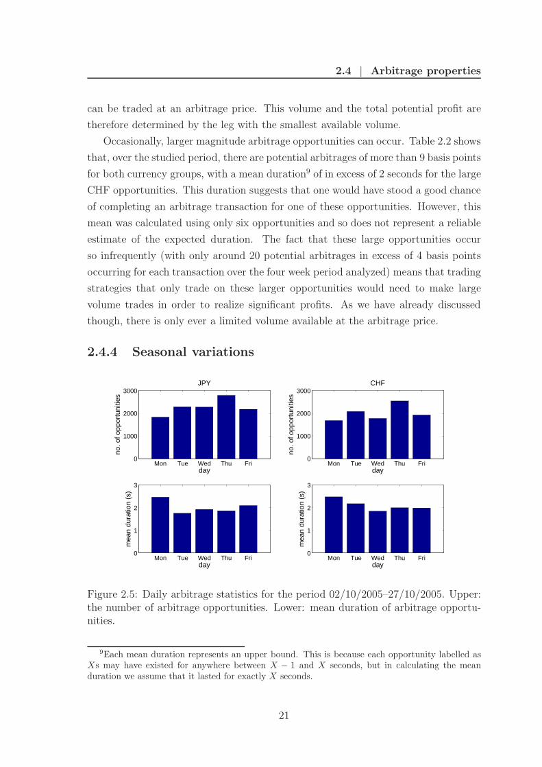
2.4.4 Seasonal variations
Mon Tue Wed Thu Fri0
1000
2000
3000
day
no. o
f opp
ortu
nitie
s
JPY
Mon Tue Wed Thu Fri0
1000
2000
3000
day
no. o
f opp
ortu
nitie
s
CHF
Mon Tue Wed Thu Fri0
1
2
3
day
mea
n du
ratio
n (s
)
Mon Tue Wed Thu Fri0
1
2
3
day
mea
n du
ratio
n (s
)
Figure 2.5: Daily arbitrage statistics for the period 02/10/2005–27/10/2005. Upper:the number of arbitrage opportunities. Lower: mean duration of arbitrage opportu-nities.
9Each mean duration represents an upper bound. This is because each opportunity labelled asXs may have existed for anywhere between X − 1 and X seconds, but in calculating the meanduration we assume that it lasted for exactly X seconds.
21
Chapter 2 | Triangular Arbitrage in the FX Market
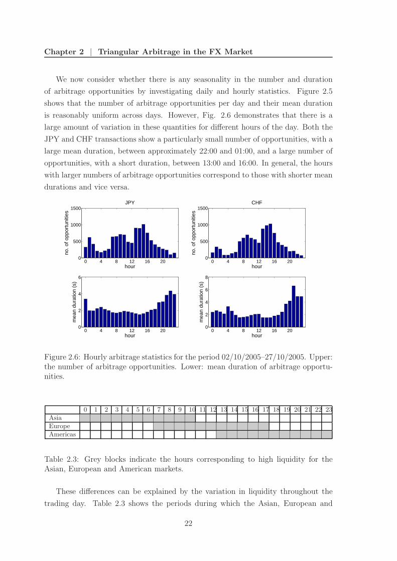
We now consider whether there is any seasonality in the number and duration
of arbitrage opportunities by investigating daily and hourly statistics. Figure 2.5
shows that the number of arbitrage opportunities per day and their mean duration
is reasonably uniform across days. However, Fig. 2.6 demonstrates that there is a
large amount of variation in these quantities for different hours of the day. Both the
JPY and CHF transactions show a particularly small number of opportunities, with a
large mean duration, between approximately 22:00 and 01:00, and a large number of
opportunities, with a short duration, between 13:00 and 16:00. In general, the hours
with larger numbers of arbitrage opportunities correspond to those with shorter mean
durations and vice versa.
0 4 8 12 16 200
500
1000
1500
hour
no. o
f opp
ortu
nitie
s
JPY
0 4 8 12 16 200
500
1000
1500
hour
no. o
f opp
ortu
nitie
s
CHF
0 4 8 12 16 200
2
4
6
hour
mea
n du
ratio
n (s
)
0 4 8 12 16 200
2
4
6
8
hour
mea
n du
ratio
n (s
)
Figure 2.6: Hourly arbitrage statistics for the period 02/10/2005–27/10/2005. Upper:the number of arbitrage opportunities. Lower: mean duration of arbitrage opportu-nities.
0 1 2 3 4 5 6 7 8 9 10 11 12 13 14 15 16 17 18 19 20 21 22 23AsiaEuropeAmericas
Table 2.3: Grey blocks indicate the hours corresponding to high liquidity for theAsian, European and American markets.
These differences can be explained by the variation in liquidity throughout the
trading day. Table 2.3 shows the periods during which the Asian, European and
22

2.4 | Arbitrage properties
American FX markets are at their most liquid. The period of highest liquidity is
from 08:00–16:00; over almost all of this period two of the markets are highly liquid
at similar time. The period of least liquidity is from around 22:00–01:00. The hours
with the largest number of arbitrage opportunities and the shortest mean durations
in Fig. 2.6 thus correspond to the periods of highest liquidity. This observation of
more arbitrage opportunities during the periods of highest liquidity seems counter-
intuitive but can be explained as follows. During liquid periods the bid-ask spread is
narrower (see Fig. 2.1) and prices move around at a higher frequency due to the large
volume of trading. This results in more price mis-alignments and consequently more
potential arbitrages. The high trade frequency, however, also ensures that the mis-
pricings are quickly traded away or removed and that any arbitrage opportunities are
short-lived. In contrast, during less liquid periods the spread is wider and the trading
volume lower which leads to fewer arbitrage opportunities. The smaller number of
traders available to correct any mis-pricings during less liquid times also results in
the arbitrages having longer durations.
2.4.5 Annual variations
The analysis so far has focused on a four week period in October 2005. We now
consider how the number and distribution of triangular arbitrage opportunities has
changed over the years by comparing results for the weeks 27/10/2003–31/10/2003,
01/11/2004–05/11/2004 and 17/10/2005–21/10/2005. These three weeks all fall at
the same time of year, so any seasonal factors are eliminated.
Transaction Year No. arbitragesPercentage of opportunities Rate product statistics
1s 2s 3s 4s 5s > 5s mean stand. dev.2003 4, 220 40 30 14 6 3 7 0.999625 4.32 × 10⁻⁴
JPY 2004 3, 662 49 28 12 5 3 3 0.999723 2.25 × 10⁻⁴
2005 2, 963 62 21 7 4 3 3 0.999758 2.17 × 10⁻⁴
2003 3, 590 41 29 13 6 4 7 0.999549 6.02 × 10⁻⁴
CHF 2004 3, 441 49 27 11 5 3 5 0.999663 3.54 × 10⁻⁴
2005 2, 672 64 20 8 3 1 4 0.999725 3.10 × 10⁻⁴
Table 2.4: Comparison of the number and percentage of arbitrage opportunities ofselected durations and the mean and standard deviation of the rate product for the pe-riods 27/10/2003–31/10/2003, 01/11/2004–05/11/2004 and 17/10/2005–21/10/2005.An opportunity labelled as Xs lasted for more than X − 1 but less than X seconds.
Table 2.4 shows that the number of arbitrage opportunities decreased from 2003–
2005 for the JPY and CHF transactions. This can be explained by the increasingly
wider use of electronic trading platforms and trading algorithms over this period.
23

Chapter 2 | Triangular Arbitrage in the FX Market
0.9980 0.9985 0.9990 0.9995 1.0000 1.0005 1.00100
0.02
0.04
0.06
0.08
0.1
0.12
0.14
γ
obse
rved
pro
babi
lity
JPY
0.9980 0.9985 0.9990 0.9995 1.0000 1.0005 1.0010
10−4
10−2
γ
obse
rved
pro
babi
lity
0.9980 0.9985 0.9990 0.9995 1.0000 1.0005 1.00100
0.02
0.04
0.06
0.08
0.1
0.12
γ
obse
rved
pro
babi
lity
CHF
0.9980 0.9985 0.9990 0.9995 1.0000 1.0005 1.0010
10−4
10−2
γ
obse
rved
pro
babi
lity
200320042005
Figure 2.7: Comparison of the rate product distributions for the periods 27/10/2003–31/10/2003, 01/11/2004–05/11/2004 and 17/10/2005–21/10/2005. Lower: distribu-tions on a log-linear scale.
These systems enabled traders to execute trades faster and to react more quickly
to price changes, which in turn gave rise to increased trading efficiency, fewer mis-
pricings and fewer triangular arbitrage opportunities. Table 2.4 also demonstrates the
significant effect that this increased execution speed had on the duration of arbitrage
opportunities. From 2003–2005, the proportion of opportunities lasting less than 1
second increased from 40% to 62% for the JPY transactions and from 41% to 64%
for the CHF transactions; and the proportion of opportunities lasting in excess of 5
seconds halved for both sets of transactions.
The distributions in Fig. 2.7 and the distribution statistics in Table 2.4 provide
further evidence of the increased pricing efficiency of the FX market from 2003 to
2005. Over this period the distribution of rate products became concentrated in
a sharper peak, with a smaller standard deviation and mean closer to one, which
demonstrates that triangular parity held a larger proportion of the time.
2.5 Profitability
We provide further insights into the profitability of trading on triangular arbitrage
signals by running simulations to determine the profit or loss that could potentially be
achieved using different trading strategies. For the full time series of JPY and CHF
24
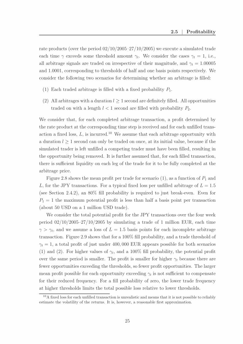
2.5 | Profitability
rate products (over the period 02/10/2005–27/10/2005) we execute a simulated trade
each time γ exceeds some threshold amount γt. We consider the cases γt = 1, i.e.,
all arbitrage signals are traded on irrespective of their magnitude, and γt = 1.00005
and 1.0001, corresponding to thresholds of half and one basis points respectively. We
consider the following two scenarios for determining whether an arbitrage is filled:
(1) Each traded arbitrage is filled with a fixed probability P1.
(2) All arbitrages with a duration l ≥ 1 second are definitely filled. All opportunities
traded on with a length l < 1 second are filled with probability P2.
We consider that, for each completed arbitrage transaction, a profit determined by
the rate product at the corresponding time step is received and for each unfilled trans-
action a fixed loss, L, is incurred.10 We assume that each arbitrage opportunity with
a duration l ≥ 1 second can only be traded on once, at its initial value, because if the
simulated trader is left unfilled a competing trader must have been filled, resulting in
the opportunity being removed. It is further assumed that, for each filled transaction,
there is sufficient liquidity on each leg of the trade for it to be fully completed at the
arbitrage price.
Figure 2.8 shows the mean profit per trade for scenario (1), as a function of P1 and
L, for the JPY transactions. For a typical fixed loss per unfilled arbitrage of L = 1.5
(see Section 2.4.2), an 80% fill probability is required to just break-even. Even for
P1 = 1 the maximum potential profit is less than half a basis point per transaction
(about 50 USD on a 1 million USD trade).
We consider the total potential profit for the JPY transactions over the four week
period 02/10/2005–27/10/2005 by simulating a trade of 1 million EUR, each time
γ > γt, and we assume a loss of L = 1.5 basis points for each incomplete arbitrage
transaction. Figure 2.9 shows that for a 100% fill probability, and a trade threshold of
γt = 1, a total profit of just under 400, 000 EUR appears possible for both scenarios
(1) and (2). For higher values of γt, and a 100% fill probability, the potential profit
over the same period is smaller. The profit is smaller for higher γt because there are
fewer opportunities exceeding the thresholds, so fewer profit opportunities. The larger
mean profit possible for each opportunity exceeding γt is not sufficient to compensate
for their reduced frequency. For a fill probability of zero, the lower trade frequency
at higher thresholds limits the total possible loss relative to lower thresholds.
10A fixed loss for each unfilled transaction is unrealistic and means that it is not possible to reliablyestimate the volatility of the returns. It is, however, a reasonable first approximation.
25

Chapter 2 | Triangular Arbitrage in the FX Market
21.5
10.5
0
00.20.40.60.81−2
−1.5
−1
−0.5
0
0.5
loss per unfilled arbitrage, Lfill probability, P1
mea
n pr
ofit
per
trad
e
−2
−1.5
−1
−0.5
0
0.5
−2
−1.5
−1
−0.5
0
Figure 2.8: Mean profit/loss per trade (in basis points) as a function of the probabilityof a transaction being filled at an arbitrage price and the loss incurred on missedarbitrages for JPY transactions over the period 10/02/2005–10/27/2005. We assumea trade threshold γ = 1 and scenario (1). The grey curve shows the break-even fillprobabilities. The probabilities are averaged over 100 simulations.
In order to achieve the 400, 000 EUR profit, it would have been necessary to stake
1 million EUR more than 17, 000 times. If we estimate transaction fees and settlement
costs at 2 EUR per trade, then each arbitrage transaction costs 6 EUR. The total
cost of 17, 000 transactions is then 102, 000 EUR, which is a significant proportion
of the potential profits. This profit is also likely to be a significant over-estimate.
In the simulations, we assumed that each arbitrage transactions is completed for
the full 1 million EUR initially staked. As discussed in Section 2.4.3, however, the
amount available at the arbitrage price is limited and may be less than this amount.
More importantly, a 100% fill probability is extremely unrealistic and in practice
the achievable fill probability will be significantly smaller. At a still unrealistic fill
probability of P2 = 0.8, for scenario (2), the potential profit is reduced to around
100, 000 EUR. This potential profit is already less than the estimated transaction
costs and there are additional infrastructure costs that also need to be considered.
2.6 Fill probabilities
Finally, we investigate the fill probabilities in more detail to provide more insight
into the chances of completing an arbitrage transaction. For scenario (1), consider a
26

2.6 | Fill probabilities
0 0.2 0.4 0.6 0.8 1−18
−16
−14
−12
−10
−8
−6
−4
−2
0
2
4x 10
5
fill probability, P1
prof
it, Π
1
0 0.2 0.4 0.6 0.8 1−10
−8
−6
−4
−2
0
2
4x 10
5
fill probability, P2
prof
it, Π
2
γt=1
γt=1.00005
γt=1.0001
Figure 2.9: Total profit (in EUR) for JPY transactions over the period 02/10/2005–27/10/2005. Each arbitrage transaction is traded with an initial currency outlay of 1million EUR and each completed transaction is filled for the full traded volume. Weassume a fixed loss L = 1.5 basis points for each incomplete arbitrage transaction.Left: scenario (1). Right: scenario (2). Error bars indicate the standard deviationin the profit over 100 simulations. The standard deviations in the profit for P1 = 0,P1 = 1, P2 = 0, and P2 = 1 are zero because the same arbitrage opportunities arefilled for each simulation.
27

Chapter 2 | Triangular Arbitrage in the FX Market
trading strategy in which a volume V is traded on each of Na arbitrage opportunities
exceeding a threshold γt over some time interval W . The total potential profit Π1
over this interval is then given by
Π1 = NaV [P1〈γ − 1|γ > γt〉 − (1 − P1)L] , (2.4)
where 〈γ − 1|γ > γt〉 denotes the average value of γ − 1 over the interval W given
that γ > γt, and the break-even fill probability P b1 (found when Π1 = 0) is given by
P b1 =
[
1 +〈γ − 1|γ > γt〉
L
]−1
. (2.5)
The break-even fill probability P b1 is therefore independent of the number of arbitrage
opportunities and decreases with increasing 〈γ − 1|γ > γt〉. This can be seen in Fig.
2.10 where the break-even fill probabilities are smaller for larger γt. For scenario (2),
we take Na = ng + n, where ng is the number of opportunities over W that last for
l ≥ 1 second, and n the number with l < 1 second. The total profit Π2 is then given
by
Π2 = ngV 〈γ − 1|γ > γt, l ≥ 1〉 + nV [P2〈γ − 1|γ > γt, l < 1〉 − (1 − P2)L] , (2.6)
and the break-even fill probability by
P b2 =
[
1 − ng〈γ − 1|γ > γt, l ≥ 1〉nL
] [
1 +〈γ − 1|γ > γt, l < 1〉
L
]−1
. (2.7)
For this scenario, the break-even fill probability P b2 therefore depends on the propor-
tion of arbitrage opportunities with length l ≥ 1, the mean value of the rate product
for opportunities with length l ≥ 1, and the mean rate product for opportunities with
l < 1.
Figure 2.10 shows break-even fill probabilities generated by trading simulations
and highlights the fact that P b2 is lower than P b
1 , for the corresponding loss, and that
the break-even fill probabilities tend to be slightly lower for the CHF than for the
JPY transactions. This difference is most marked for scenario (2), with γt = 1.0001.
In this case, if a fixed loss of 2 basis points per unfilled arbitrage is assumed, a fill
probability of only 17% is needed to break-even.
Although this fill probability seems low, it would nevertheless be difficult to
achieve. Consider a strategy where a similar fill probability of 20% is required to
break-even. This implies that one would need to be filled on 1 in 5 of the arbitrage
opportunities traded on. If there are 5 market participants trading on each oppor-
tunity, each able to transact at the same speed, then this fill frequency is feasible.
28

2.6 | Fill probabilities
2 1.5 1 0.5 00
0.1
0.2
0.3
0.4
0.5
0.6
0.7
0.8
0.9
1
loss per unfilled arbitrage, L
brea
k−ev
en fi
ll pr
obab
ility
, P1b
JPY
2 1.5 1 0.5 00
0.1
0.2
0.3
0.4
0.5
0.6
0.7
0.8
0.9
1
loss per unfilled arbitrage, L
brea
k−ev
en fi
ll pr
obab
ility
, P1b
CHF
γt=1
γt=1.00005
γt=1.0001
2 1.5 1 0.5 00
0.1
0.2
0.3
0.4
0.5
0.6
0.7
0.8
0.9
1
loss per unfilled arbitrage, L
brea
k−ev
en fi
ll pr
obab
ility
, Pb 2
2 1.5 1 0.5 00
0.1
0.2
0.3
0.4
0.5
0.6
0.7
0.8
0.9
1
loss per unfilled arbitrage, L
brea
k−ev
en fi
ll pr
obab
ility
, P2b
Figure 2.10: The fill probability required to break-even as a function of the loss in-curred per incomplete arbitrage transaction. Upper: scenario (1). Lower: scenario(2). Error bars indicate the standard deviation in the fill probability over 100 simu-lations.
29

Chapter 2 | Triangular Arbitrage in the FX Market
However, in the FX market there are many more market participants than this com-
peting for each arbitrage opportunity, so to achieve this fill probability one would
need to identify and execute each arbitrage opportunity faster than most of these
competitors. These competitors are also likely to be continually striving to increase
their execution speeds in the electronic trading “arms race”. Given the costs asso-
ciated with staying ahead in this race, it would be extremely costly to maintain the
fastest execution speeds and to regularly beat the majority of other competitors to
the arbitrage prices over a prolonged period of time. The fill probabilities required
to realize the profits indicated in Fig. 2.9 are therefore very difficult to achieve and,
as a consequence, the profit levels are also extremely unrealistic.
The calculated fill probabilities also represent lower bounds of acceptability be-
cause to justify trading on an opportunity a trader would expect a reasonably high
expected profit and not simply to break-even. When one factors in costs such as
brokerage, the internet connections required to access the market, and the cost of
developing and supporting a sophisticated electronic trading system, the actual fill
probabilities necessary to achieve an acceptable level of profit would be substantially
higher than those calculated. It therefore appears that, although mis-pricings do ap-
pear in the FX market, an unfeasibly large fill probability would need to be achieved
over a prolonged period of time to realize any significant profits from them.
2.7 Summary
We have shown that triangular arbitrage opportunities exist in the FX market, but
the vast majority of these opportunities are less than 1 second in duration and 1 basis
point in magnitude. The longer, larger opportunities that do occur appear with a
significantly lower frequency. We showed that, somewhat counter-intuitively, more ar-
bitrage opportunities occur during periods of higher liquidity, but these opportunities
tend to be removed from the market very rapidly. The increased number of oppor-
tunities during liquid periods was attributed to the higher trading frequency, which
resulted in more mis-pricings, but also ensured that they were quickly corrected. We
have also shown that from 2003 to 2005 the market became increasingly efficient at
eliminating mis-pricings and explained this by the increased use of electronic trading
platforms, which enabled traders to react faster to price changes.
Finally, we used trading simulations to investigate the profitability of trading on
triangular arbitrage signals. Considering the strong competition for each arbitrage,
the costs of trading, and the costs required to maintain a technological advantage, it
30

2.7 | Summary
seems that a trader would need to beat other market participants to an unfeasibly
large proportion of arbitrage opportunities for triangular arbitrage to remain prof-
itable in the long-term. We therefore conclude that the FX market appears internally
self-consistent and these results provide a limited verification of FX market efficiency.
This chapter has also demonstrated the critical importance of using the correct
type of data to study financial markets. If one uses data that is inappropriate for
a particular analysis, it is easy to conclude that data artifacts represent meaningful
structure. For example, when indicative FX price data is used to investigate triangular
arbitrage, arbitrage opportunities appear to remain active in the market longer, and
to be more profitable, than when executable data is used.
31


Chapter 3
A Principal Component Analysisof Financial Market Correlations
In this chapter, we continue to investigate financial markets, but extend the analysis
to include assets from other major markets in addition to the FX market. We have
submitted a paper based on this work for publication [P5]. We return to the FX
market in Chapter 5.
3.1 Introduction
The global financial system is composed of a multitude of markets spread across
a range of geographic locations with a wide variety of assets traded in each mar-
ket. There is strong coupling between different financial markets such that the price
changes of particular assets can be driven not only by the price changes of assets
traded in the same market, but also by price changes of assets traded in other
markets. Because of the close relationships between different assets and markets,
a primary concern of market practitioners is estimating the correlations between the
changes in asset price time series. There are many reasons for wanting to understand
correlations in price movements; perhaps the most common motivation is for risk
management purposes. For a portfolio of assets, the likelihood of large losses can
be significantly higher when the assets held in the portfolio are correlated [176]; an
understanding of the correlation between different financial instruments can therefore
help in managing the risk associated with a portfolio. The standard approach for
representing the correlations of a group of financial assets is to calculate the linear
correlation coefficient between pairs of assets. However, for N assets, this results in12N(N −1) correlation coefficients, so simultaneous investigation of these interactions
33

Chapter 3 | Financial Market PCA
is difficult for even moderate N . Attaining an understanding of the market system
therefore necessitates some form of simplification.
In this chapter, we simplify the analysis of financial market correlations by ex-
tracting common features using PCA. We first coarse-grain the correlation matrix by
identifying the principal components (PCs) that account for a large proportion of the
variability of the system. We then characterize the evolving relationships between
the different assets by analyzing the correlations between the asset price times series
and PCs. By focusing on correlations between the price time series and PCs, we
significantly reduce the number of correlations that we need to consider to attain
an understanding of the system. Using this approach, we uncover notable changes
that occurred in financial markets and we identify the assets that were significantly
affected by these changes.
3.1.1 Components and factors
It has been widely observed that price time series for different financial assets display
similar characteristics and, because the prices often depend on the same economic
data and market signals, it is often hypothesized that financial time series can be
decomposed into common drivers or factors [296]. The aim of factor modelling in
finance is to try to identify these factors. Several approaches to factor modelling
are closely related to PCA and some use PCA as a tool for identifying factors [63].
Because of the close ties between the two techniques, we provide an overview of
factor modelling in this section. We highlight, however, that there is an important
difference between what we are trying to achieve using PCA and the objective of factor
modelling. In factor modelling, the aim is to identify a number of “fundamental”
market factors that drive asset prices; these factors can be unobservable and often
factor models incorporate random errors that represent the variability in the system
not explained by the factors. In contrast, we use PCA to produce a parsimonious
representation of market correlations and we make no assumptions about whether the
components that we identify correspond to fundamental market variables. In fact, it
is likely that the PCs are themselves a combination of several underlying factors.
3.1.1.1 Factor models
Factor models can be separated into two classes: confirmatory and exploratory. Al-
though this classification is slightly fuzzy, it helps to illustrate the different techniques.
Many of these models assume that the observed price series can be written as lin-
ear combinations of common factors. In confirmatory factor modelling, a number
34

3.1 | Introduction
of indicator variables are selected that are posited to drive the observed price time
series and a factor model is constructed to test this prediction. There are two main
types of confirmatory factor models in finance [296]: macroeconomic and fundamen-
tal models. Macroeconomic factor models attempt to explain the behaviour of asset
returns using macroeconomic variables, such as interest rates and GDP growth rates.
The relationship between these indicator variables and the observed assets is usually
determined using linear regression. Fundamental factor models try to explain price
movements using fundamental properties of the assets; for example, using properties
such as market capitalization and industrial sector to explain equity price movements.
Again, the relationships between the indicator variables and the observed assets are
usually determined using linear regression [63, 296].
3.1.1.2 Principal component and factor analysis
The second class of factor models are exploratory methods. In contrast to confir-
matory models, exploratory methods make no assumptions about which variables
correspond to the underlying factors; instead, the factors are estimated directly from
the asset return time series. Two widely used exploratory techniques are factor anal-
ysis1 (FA) and PCA [63, 301]. The two names are often used interchangeably in the
literature and the two approaches share the common goal of reducing a set of N
observed variables to a set of m < N new variables [301]. However, there are clear
distinctions between the two techniques.
In FA the aim is first to identify factors that are common to two or more variables
and these factors can either be correlated or uncorrelated. In addition to the common
factors, a set of unique factors are also identified that are specific to each variable and
orthogonal to each other and to all of the common factors [103]. In PCA the PCs are
identified on the basis of variance. The first component accounts for as much of the
variance in the system as possible, the second as much of the remaining variance as
possible, and so on. In PCA the components are chosen such that they are mutually
orthogonal and account for all of the variability in the system; there are no unique
components specific to particular variables.
The differences between PCA and FA can be better understood by considering
the decomposition of the covariance matrix of the observed variables in the two cases.
If we let Z represent an N × T matrix of T observations of the return time series of
1Note the distinction between factor modelling and factor analysis – factor analysis is a type offactor modelling.
35
Chapter 3 | Financial Market PCA
N assets, for FA the covariance matrix ΣZ of Z can be written as
ΣZ = ΩFΣFΩTF − ε2, (3.1)
where ΩF is a matrix of common factor weights, ΣF is the covariance matrix of the
common factors, ε2 is a diagonal matrix of unique factor variances, and T indicates a
matrix transpose. Using PCA the covariance matrix ΣZ can be written as
ΣZ = ΩΣYΩT , (3.2)
where Ω is the matrix of PC coefficients and ΣY is the covariance matrix of the
principal components.2 Equations 3.1 and 3.2 highlight the key differences between
the two models. The additional term ε2 in the FA equation allows for specific factors
that are unique to particular observed variables [297]. In contrast, PCA does not
explicitly allow for unique factors, instead the components represent both unique and
common variance. The components identified using PCA therefore account for all of
the variability of the system, whereas the common factors in FA often do not.
There is some debate on the relative merits of FA and PCA for factor modelling
and on whether the outputs of the two methods are equivalent [297,301,307]. Because
it is not our objective to use PCA to derive a factor model in this chapter, it is not
necessary to perform a comprehensive comparison of the two techniques. Neverthe-
less, it is instructive to highlight some of the main performance differences. It is often
argued that one of the major advantages of PCA over FA is the relative simplicity of
the process of fitting the model [160, 297] and, in fact, some FA techniques use PCA
as just a first step in the process of identifying the factors [103]. Another argument
used in support of PCA is that it is able to identify the elements in the matrix Ω (to
within a sign), whereas the entries in ΩF cannot be determined exactly [297]. Despite
these differences, it has been noted that the two methods produce very similar results
if the error terms in the factor model all have the same variance [66, 72]. In fact, it
can be seen from Eqs. 3.1 and 3.2 that when the unique variances are zero, the two
models are equivalent.
In this chapter, we use PCA in the same way that it is employed in factor mod-
elling: to decompose the correlation matrix of multiple assets into a few explanatory
variables. However, in contrast to factor modelling, we use PCA simply to charac-
terize the changing correlation structures within markets and do not assume that the
components that we identify are fundamental market factors. To emphasize this, we
refer to components rather than factors.
2We discuss this equation in more detail in Section 3.3.
36

3.1 | Introduction
PCA is a well established tool in data analysis for generating lower-dimensional
representations of multivariate data [159] and has provided useful insights in a diverse
range of fields, including chemistry, e.g., [89], genetics, e.g., [245], psychology, e.g.,
[252], and astrophysics, e.g., [149]. In finance, PCA has been used to identify common
factors in international bond returns, e.g., [81, 237] and in equity returns, e.g., [159,
296], and has been applied to other problems, such as arbitrage pricing theory, e.g.,
[66, 72], portfolio theory, e.g., [298], and to produce market indices, e.g., [101].
3.1.2 Random matrix theory
PCA is closely linked to random matrix theory (RMT), which was originally devel-
oped by Wigner to deal with the statistics of the energy levels of many-body quantum
systems [308]. Wigner replaced the Hamiltonian of the system under investigation by
an ensemble of random Hamiltonians (given by real symmetric matrices with inde-
pendent random elements), which were considered to describe the generic properties
of the system [137]. Using this method he successfully described the spectra of atomic
nuclei and complex atoms. Subsequently, RMT has become an important tool in a
wide range of other areas, including quantum field theory and two-dimensional grav-
ity [137, 206], and recently in finance, e.g., [176, 239].
The standard financial approach is to compare the eigenvalues and eigenvectors of
an empirical correlation matrix of asset returns with correlation matrices generated
using time series of randomly distributed returns and with analytic distributions from
RMT. The bulk of the eigenvalues of empirical correlation matrices are found to fall
within the range predicted by RMT, which is usually taken as an indication that to
a large extent the correlation matrix is random and dominated by noise. Further, it
has been found that the smallest eigenvalues of the empirical correlation matrix are
most sensitive to noise and, because the eigenvectors corresponding to the smallest
eigenvalues are used to determine the least risky portfolios in Markowitz portfolio
theory [199], this has implications for risk management [166, 176, 238, 239]. For ex-
ample, if one holds a portfolio of two assets with highly correlated price movements,
a decrease in the value of one of the assets is likely to be accompanied by a decrease
in value of the other asset. If the assets in a portfolio are highly correlated, there is
therefore a higher risk of a significant decrease in the portfolio value. This risk would
be lower if there were a small correlation between the asset values. An understanding
of correlations in asset price movements is therefore an important part of successful
risk management and optimal portfolio selection [166,176,199,238,239]. The degree
37

Chapter 3 | Financial Market PCA
to which it is possible to diversify risk is intrinsically linked to the number of com-
mon factors. If there are only a few significant factors driving markets, one would
expect asset prices to be highly correlated and for it to be more difficult for market
practitioners to hold diversified portfolios and consequently to lower their investment
risk.
Prior studies of financial market price data using RMT and PCA have focused on
specific markets. For example, there is a large body of work analyzing equity markets,
e.g., [166, 176, 238, 239], and there have also been investigations of emerging market
equities, e.g., [64,235,309], the FX market, e.g., [82], and bond markets, e.g., [81,237].
Most prior studies only analyze a single correlation matrix and do not investigate the
temporal evolution of correlations. However, changes in correlations are of critical
importance in many financial applications; for example, changes in the extent to
which assets held in a portfolio are correlated can have a significant impact on the
risk associated with the portfolio. The work in this chapter differs from prior studies
by investigating a diverse range of asset classes and by studying the evolution of the
correlations between these assets. By studying the time dynamics of the correlations,
we uncover periods during which there were major changes in the correlation structure
of markets and identify the assets affected by these changes.
3.2 Data
3.2.1 Description
We study correlations for a wide variety of markets, but several factors limit the
assets that we can include. For example, for some time series there are a large
number of missing data points. One solution to this problem is to fill-in the missing
data by interpolating between the data points that we do have, but this approach
is inappropriate when there are several consecutive missing data points. A second
reason for excluding time series is that they begin too recently. In this study, we use
time series beginning in January 1999 because this time interval contains periods of
very different market behaviour that we can compare. However, data is only available
for some instruments for a few years. For example, although some emerging market
corporate bond indices are now published, they have only been published since 2005
and consequently we do not include them. Other time series are complete and cover
the full time period, but are excluded because of the nature of the data. For example,
38

3.2 | Data
we exclude any exchange rate that has been pegged3 for any of the studied period.
The peg implies that the value of the pegged exchange rate can be determined using
the rate (or rates) to which it is pegged, so the pegged rate is redundant.
Taking all of these factors into account, we include time series for 98 financial
products from all of the major markets. This includes 25 developed market equity
indices, 3 emerging market equity indices, 4 corporate bond indices, 20 government
bond indices, 15 exchange rates, 9 metals, 4 fuel commodities, and 18 other com-
modities. (See Table A.1 in Appendix A for a description of all of the assets that we
include.) For many markets, we study indices rather than specific assets so that we
have an aggregate view of the market.4 For all of the commodities, we use futures5
contracts because commodities are most widely traded in the futures market. How-
ever, for single futures contracts, the price time series will have a discontinuity at the
contract expiry date. To minimize this discontinuity, we use the “Generic 1st futures”
contract for each commodity, which is the price of the nearest dated futures contract
(i.e., the contract with the closest expiry date).
We include assets from a range of geographical regions, so many are traded during
different hours of the day. For example, stocks included in the Nikkei 225 are traded
on the Tokyo Stock Exchange, which operates between midnight and 6 AM GMT,
whereas stocks included in the FTSE 100 index are traded on the London Stock
Exchange, which operates between 8 AM and 4:30 PM GMT. To minimize any effects
resulting from the non-synchronicity of the price time series for markets from different
time zones, we use weekly price data. We take the weekly price of an asset to be the
last price posted each week. In this study, we investigate the period from 08/01/1999–
01/01/2010 and we have 575 prices for each asset.
3A pegged exchange rate is an exchange rate regime wherein a currency’s value is matched tothe value of a single currency or a basket of currencies.
4By using indices the data is also representative of a larger set of assets than if we included timeseries for individual assets. For example, if we studied individual equities, we would need to includeseveral stocks from each industrial sector to obtain a representative cross-section of the market;however, we can only include a limited number of assets in the analysis. We discuss the reasons forthis in Section 3.2.3.
5A future is a standardized contract to buy or sell an asset at a specified future date at a priceagreed on the day that the contract is entered in to.
39

Chapter 3 | Financial Market PCA
3.2.2 Returns
We denote the price of asset i at discrete time t as pi(t), i = 1, . . . , N , and define a
logarithmic return zi(t) for asset i between consecutive time steps as6
zi(t) = ln
[
pi(t)
pi(t − 1)
]
. (3.3)
In Fig. 3.1, we show that there are large differences between the return distributions
for assets from different classes. For example, returns for U.S. government bonds are
concentrated in a sharp peak around zero, whereas the distribution for oil has much
more weight in the tails as a result of regular large moves in the oil price.
In calculating a correlation coefficient for a pair of time series, it is important to
ensure that the time series are stationary [134]. We study returns rather than prices
because, in general, return time series are close to stationary whereas price time series
are not [73]. This can be demonstrated by considering the autocorrelation function
(acf) of the two types of time series. The autocorrelation αi of a time series zi is given
by
αi(τ) =
∑T−τt=1
[
zi(t) − 〈zi〉][
zi(t + τ) − 〈zi〉]
∑Tt=1
[
zi(t) − 〈zi〉]2 , (3.4)
where 〈· · · 〉 indicates a time average over T − τ returns and τ is the lag between time
steps over which the autocorrelation is calculated. For stationary time series, the acf
decays rapidly with increasing lag, but this is usually not the case for non-stationary
series [73]. In Fig. 3.2(a), we demonstrate for the EUR/USD exchange rate that the
return time series acf decays rapidly, whereas the price time series decays slowly. In
Fig. 3.2(b), we show that the return time series for all of the studied assets decay
rapidly, with most values falling within the 95% confidence bounds for Gaussian white
noise.7 The rapid decay of the acfs of the return time series suggests that the return
process is stationary, which implies that these time series are suitable for investigating
market correlations.
6An alternative return is the arithmetic return which is defined as zai (t) = [pi(t)−pi(t−1)]/pi(t−
1). This is equal to the first term in the Taylor expansion of the logarithmic return, so arithmetic andlogarithmic returns are approximately equal for small returns. Logarithmic returns are, however,often used instead of arithmetic returns because logarithmic returns are symmetric [73]. For example,an investment of £100 that yields an arithmetic return of 50% followed by an arithmetic return of-50% results in £75. In contrast, an investment of £100 that yields a logarithmic return of 50%followed by an logarithmic return of -50% results in £100.
7We note that there are two spikes in the acf for frozen pork bellies (PB1) at 26 and 52 weeklags, which suggests that there is an interesting periodicity in this return time series.
40

3.2 | Data
−0.1 −0.05 0 0.05 0.1 0.150
0.1
0.2
0.3
0.4
0.5
z
obse
rved
pro
babi
lity
USGATRMOODCAASPXGBP/USDXAUCO1
Figure 3.1: Observed return distributions for the period 08/01/1999–24/07/2009.We show the S&P equity index (SPX), a U.S. government bond index (USGATR),a AA-rated corporate bonds index (MOODBAA), the sterling-dollar exchange rate(GBP/USD), gold (XAU), and crude oil futures (CO1).
0 20 40 60 80 100−0.2
0
0.2
0.4
0.6
0.8
1
τ
α
0 20 40 60 80 100−0.2
0
0.2
0.4
0.6
0.8
1
τ
α
b)a)
Figure 3.2: a) Comparison of the autocorrelation function for the EUR/USD price(upper green line) and return (lower blue line) time series. The horizontal red linesshow the 95% confidence intervals assuming Gaussian white noise. b) Autocorrelationfunctions for all of the studied return time series. The horizontal red lines show the95% confidence intervals assuming Gaussian white noise.
41
Chapter 3 | Financial Market PCA
3.2.3 Correlations
To simplify the notation for the definition of the empirical correlation matrix, we
define a standardized return as
zi(t) =zi(t) − 〈zi〉
σ(zi), (3.5)
where σ(zi) =√
〈z2i 〉 − 〈zi〉2 is the standard deviation of zi over a time window of
T returns and 〈· · · 〉 indicates a time average over T . We represent the standardized
returns as an N × T matrix Z, so the empirical correlation matrix R is given by
R =1
TZZT , (3.6)
and has elements r(i, j) that lie in the interval [−1, 1]. Note that, because we have
standardized the time series, the correlation matrix R of returns Z is equal to the
covariance matrix ΣZ
of Z.
We create an evolving sequence of correlation matrices by rolling the time window
of T returns through the full data set. The choice of T is a compromise between
overly noisy and overly smoothed correlation coefficients [227, 229], but is usually
chosen such that Θ = T/N ≥ 1.8 In this study, we fix T = 100 (each window then
contains just under two years of data and Θ = 1.02) and we roll the time window
through the data one week at a time. By only shifting the time window by one data
point, there is a significant overlap in the data contained in consecutive windows;
however, this approach enables us to track the evolution of the market correlations
and to identify time steps at which there were significant changes in the correlations.
The choice of T results in 452 correlation matrices for the period 1999–2010.
3.2.3.1 Correlations for all assets
In Fig. 3.3, we show the distribution of empirical correlation coefficients aggregated
over all time windows. To highlight any interesting features in the correlations, we
compare the distribution to corresponding distributions for simulated random returns
and randomly shuffled returns. We generate shuffled data by randomly reordering
the full return time series for each asset independently. This process destroys the
temporal correlations between the return time series, but preserves the distribution of
returns for each series. We then produce correlation matrices for the shuffled returns
by rolling a time window of T returns through the shuffled data and calculating a
8We discuss the compromise between overly noisy and overly smoothed correlations in more detailin Section 5.2.2
42

3.2 | Data
correlation matrix for each position of the window. We produce simulated data by
independently generating N time series of returns (where each series is the same
length as the original data) whose elements are drawn from a Gaussian distribution
with mean zero and unit variance. We again roll a time window of length T through
the data and calculate a correlation matrix for each window.
Figure 3.3 shows that the distribution of correlation coefficients for the market
data is significantly different to the two random distributions, with more large positive
and negative correlations for market returns. The differences between the distribu-
tions demonstrate that there are temporal correlations between returns for financial
assets that are incompatible with the random null models that we consider.
−1 −0.8 −0.6 −0.4 −0.2 0 0.2 0.4 0.6 0.8 10
0.01
0.02
0.03
0.04
0.05
0.06
0.07
0.08
r
obse
rved
pro
babi
lity
observedshuffledsimulated
Figure 3.3: Distribution of correlation coefficients r(i, j) aggregated over all timewindows for the observed, shuffled and simulated data.
3.2.3.2 Intra-asset-class correlations
Figure 3.3 shows the distribution of correlations between the return time series of
all assets, but it is instructive to disaggregate this distribution and to consider only
correlations between assets in the same class. In Fig. 3.4 we show that there are clear
differences in the intra-class correlations for different assets. For example, corporates
bonds and government bonds tend to be highly correlated, whereas many of the
assets within the “other commodities” class are uncorrelated (which is unsurprising
given the variety of commodities that we include in this class). The distributions
of correlation coefficients for all of the asset classes deviate from the distributions
43

Chapter 3 | Financial Market PCA
expected for random returns. The deviations from random distributions imply that
financial market correlation matrices contain structure that warrants investigation.
−1 0 10
0.1
0.2
0.3
0.4
obse
rved
pro
babi
lity
government
−1 0 10
0.2
0.4
0.6
0.8
1corporate
−1 0 10
0.1
0.2
0.3
0.4equities
−1 0 10
0.1
0.2
0.3
0.4currencies
−1 0 10
0.1
0.2
0.3
0.4metals
−1 0 10
0.1
0.2
0.3
0.4
r
fuels
−1 0 10
0.1
0.2
0.3
0.4other commodities
Figure 3.4: The distribution of correlation coefficients r(i, j) between the return timeseries for assets within each class aggregated over all time windows.
3.3 Principal component analysis
We investigate the structure of the correlation matrices using PCA. The aim of PCA
is to find the linear transformation Ω that maps a set of observed variables Z into a
set of uncorrelated variables Y [159]. We define the N × T matrix Y as
Y = ΩZ, (3.7)
where each column yk (k = 1, . . . , N) corresponds to a PC of Z and the transformation
matrix Ω has elements ωij. The first row ω1 of Ω (which contains the first PC
coefficients) is chosen such that the first PC y1 is aligned with the direction of maximal
variance in the N -dimensional space defined by Z. Each subsequent PC accounts for
as much of the remaining variance of Z as possible, subject to the constraint that the
ωk are mutually orthogonal. We further constrain the vectors ωk such that ωkωTk = 1
for all k.
The correlation matrix R is an N ×N diagonalizable, symmetric matrix that can
be written in the form
R =1
TEDET , (3.8)
44

3.3 | Principal component analysis
where D is a diagonal matrix of eigenvalues βk and E is an orthogonal matrix of its
eigenvectors. It can be shown [159] that the eigenvectors of the correlation matrix
correspond to the directions of maximal variance such that Ω = ET and the PCs are
easily found through the diagonalization in Eq. 3.8.9 We note that the signs of the
PCs are arbitrary; if the sign of every coefficient in a component yk is reversed, the
variance of yk and the orthogonality of ωk with all of the other eigenvectors does not
change.
3.3.1 Eigenvalues
In Section 3.1.2, we highlighted the close links between RMT and PCA. A standard
financial application of RMT is to compare the eigenvalues of the correlation matrix
of market returns with the distribution of eigenvalues for random matrices, e.g., [176,
239]. Any deviations from the predictions of RMT are usually considered to indicate
non-random, and potentially insightful, structure in the correlation matrix [176,239].
The correlation matrix for N mutually uncorrelated time series of length T with
elements drawn from a Gaussian distribution is a Wishart matrix [176, 239]. In the
limit N → ∞, T → ∞, and with the constraint that Θ = T/N ≥ 1, the probability
density function ρ(β) of the eigenvalues β of such correlation matrices is given by [269]
ρ(β) =Θ
2πσ2(Z)
√
(β+ − β)(β− − β)
β, (3.9)
where σ2(Z) denotes the variance of the elements of Z, and β+ and β− are the maxi-
mum and minimum eigenvalues and are given by
β± = σ2(Z)
(
1 +1
Θ± 2
√
1
Θ
)
. (3.10)
When Θ = 1, the lower bound of the range of eigenvalues β− = 0, the upper bound
β+ = 4σ2(Z), and as β → β− = 0, the density of eigenvalues ρ(β) diverges as
∼ 1/√
β. The above results are only valid in the limit N → ∞; for finite N , the
boundaries of the eigenvalue distribution are blurred with a non-zero probability of
finding eigenvalues larger than β+ and smaller than β−. For the standardized return
matrix Z that we investigate, σ2(Z) = 1 so β+ = 4.
9PCA is sometimes performed on the covariance matrix rather than the correlation matrix.However, if there are large differences in the variances of the time series used as inputs in the PCA,the variables with the largest variances will tend to dominate the first few PCs when the covariancematrix is used. Figure 3.1 shows that there are differences in the variances of the returns for differentassets, so we use the correlation matrix. Of course, the correlation matrix is simply the covariancematrix for standardized variables.
45

Chapter 3 | Financial Market PCA
In Fig. 3.5, we compare the eigenvalue distribution for market data (aggregated
over all time windows) with the distributions for shuffled and simulated data. In
Fig. 3.5(a), we show that the eigenvalue distribution for market correlations differs
from that of random matrices.There are many eigenvalues larger than the upper bound
β+ = 4 predicted by RMT (with several eigenvalues almost 10 times as large as the
upper bound). In prior studies of equity markets, the eigenvector corresponding to
the largest eigenvalue has been described as a “market” component, with roughly
equal contributions from each of the N equities studied, and the eigenvectors cor-
responding to the other eigenvalues larger than β+ have been identified as different
market sectors [176,239]. In Section 3.5, we discuss the interpretation of the observed
eigenvectors with eigenvalues β > β+. For now, we simply note that the deviations
of the empirical distribution of eigenvalues from the predictions of RMT again im-
ply that the correlation matrices contain structure that is incompatible with the null
models that we consider.
In Figs. 3.5(b) and (c), we illustrate that the distributions for shuffled and simu-
lated data are very similar and that they agree very well with the analytical distribu-
tion given by Eq. (3.9) over most of the range of β. In particular, both distributions
have an upper bound close to the theoretical maximum β+ = 4. However, for Θ ≈ 1.02
(the value that corresponds to the selected T and N), the observed distribution of
eigenvalues for random data does not fit the distribution in Eq. (3.9) as β → 0. For
both the simulated and shuffled data, we observe a much higher probability density
near β = 0 than that predicted by RMT. The high probability density near zero is
a result of the fact that T ≈ N . When we simulate eigenvalue distributions for data
with T ≫ N , we observe a much smaller probability density near zero. In Figs. 3.5(b)
and (c), we also show the theoretical distribution for Θ = 1. In this case, ρ(β) diverges
as β → 0, which fits the randomly generated distributions reasonably well.
3.3.2 Eigenvectors
We now investigate the distribution of the elements ωij (the PC coefficients) of the
eigenvectors of the correlation matrices. We denote the ith element of the kth eigen-
vector as ωk(i) and use the standard approach of normalizing each eigenvector such
that∑N
i=1 ωk(i)2 = N [176,238,239]. Correlation matrices R are real symmetric ma-
trices, so we compare the eigenvector properties of the matrices R with those for real
symmetric random matrices. Such random matrices display the universal properties
of the canonical ensemble of matrices known as the Gaussian orthogonal ensemble
46

3.3 | Principal component analysis
0 5 10 15 20 25 30 35 400
1
2
10 20 30 4050
0.002
0.004
λ
ρ(λ)
0 0.5 1 1.5 2 2.5 3 3.5 40
2
4
λ
0 0.5 1 1.5 2 2.5 3 3.5 40
2
4
ρ(λ)
3 3.5 40
0.05
0.1
ρ(λ)
λ
3 3.5 40
0.05
0.1
λ
ρ(λ)
Q = 1.02
Q = 1
Q = 1.02
Q = 1
a)
c)
b)
Figure 3.5: The distribution of eigenvalues β of the correlation matrices aggregatedover all time windows for (a) market (b) shuffled, and (c) simulated data. In (b) and(c), we show the eigenvalue probability density functions for random matrices givenby Eq. 3.9 for Θ = 1.02 (solid red line) and Θ = 1 (dashed green line). The insetsshow the distributions of the largest eigenvalues. The distributions for shuffled (b)and simulated data (c) both have an upper bound close to the theoretical maximumβ+ = 4.
47

Chapter 3 | Financial Market PCA
(GOE) [238,239]. For the GOE, the probability density ρ(ωk) of the elements of the
kth eigenvector is a Gaussian distribution with mean zero and unit variance [137].
In Fig. 3.6, we show the distribution of elements of the eigenvectors k = 1, . . . , 6(the six components with the largest eigenvalues), k = 25, 40, 50, 75 (whose eigen-
values lie within the interval [β−, β+] for random matrices), and k = 97, 98 (the two
components with the smallest eigenvalues). We aggregate the distributions for each
eigenvector over all time windows; however, the sign of each eigenvector is arbitrary so,
to ensure that the signs of the eigenvectors are consistent through time, we choose the
sign of the kth eigenvector ωtk at time step t to maximize
∑Ni=1 sgn[ωt−1
k (i)] sgn[ωtk(i)],
where sgn[x] is the sign function.10
Figure 3.6 shows that the RMT distribution closely matches the distributions for
shuffled and simulated data, but there are differences between these distributions
and the distributions for the market correlation matrices. These differences are most
pronounced for the first and second PCs; in particular, there are asymmetries in
the distributions for market data that are not present in the random distributions.
The eigenvector distributions for eigenvalues within the interval [β−, β+] also deviate
from the predictions of RMT, which contrasts with the results of similar studies of
equity markets. In Refs. [176, 238], the distributions of elements of the eigenvectors
corresponding to eigenvalues falling within the interval [β−, β+] were found to fit a
Gaussian distribution, which was taken as an indication that these eigenvectors did
not contain any information [176]. However, the eigenvector distributions that we
observe for eigenvalues in the interval [β−, β+] have excess kurtosis compared with a
Gaussian distribution. A key difference between the analysis that we present and prior
studies is that we investigate multiple asset classes, whereas prior studies focused on
a single type of asset. The addition of inter-asset-class correlations may explain the
differences that we observe in the eigenvector distributions.
3.4 Temporal evolution
In Sections 3.3.1 and 3.3.2, we analyzed aggregate results for all time steps. The
results imply that the financial market correlation matrices that we study contain
structure that is incompatible with the random null models that we consider. We
now investigate the evolution of this structure through time.
10That is, for each time step we perform the two summations∑N
i=1sgn[ωt−1
k (i)] sgn[ωtk(i)] and
∑N
i=1sgn[ωt−1
k (i)] sgn[−ωtk(i)] and choose whichever of −ωt
k or ωtk results in the largest value for the
sum.
48

3.4 | Temporal evolution
−4 −2 0 2 40
0.2
0.4
k = 1
−4 −2 0 2 40
0.2
0.4
k = 2
−4 −2 0 2 40
0.2
0.4
k = 3
−4 −2 0 2 40
0.2
0.4
k = 4
−4 −2 0 2 40
0.2
0.4
0.6k = 5
ρ(ω
k)
−4 −2 0 2 40
0.2
0.4
0.6k = 6
−4 −2 0 2 40
0.2
0.4
0.6k = 25
−4 −2 0 2 40
0.2
0.4
0.6k = 40
−4 −2 0 2 40
0.2
0.4
0.6k = 50
−4 −2 0 2 40
0.2
0.4
0.6k = 75
ωk
−4 −2 0 2 40
0.6
1.2k = 97
−4 −2 0 2 40
0.6
1.2k = 98
observed
shuffled
RMT
Figure 3.6: The distribution ρ(ωk) of the elements ωk(i) of the i = 1, . . . , N elementsof the kth eigenvector aggregated over all time windows. We show the distributionsfor k = 1, . . . , 6 (the six eigenvectors with the largest eigenvalues), k = 25, 40, 50, 75whose eigenvalues fall within the range [β−, β+] predicted by RMT, and k = 97, 98(which have very small eigenvalues). The red line histograms show the equivalentdistributions for shuffled data and the green lines show the distribution predicted byRMT.
49

Chapter 3 | Financial Market PCA
3.4.1 Proportion of variance
We begin by investigating the eigenvalues of the correlation matrices. We can write
the covariance matrix ΣY for the PC matrix Y as
ΣY =1
TYYT =
1
TΩZZT ΩT = D. (3.11)
where D is the diagonal matrix of eigenvalues β. The total variance of the returns Z
for the N assets is then given by
N∑
i=1
σ2(zi) = tr(ΣZ) =
N∑
i=1
βi =
N∑
i=1
σ2(yi) = tr(D), (3.12)
where ΣZ
is the covariance matrix for Z and σ2(zi) is the variance of the vector zi
of returns for asset i. The proportion of the total variance in Z explained by the kth
PC is then given byσ2(yk)
∑N
i=1 σ2(zi)=
βk
β1 + . . . + βN
=βk
N, (3.13)
i.e., the ratio of the kth largest eigenvalue βk of the correlation matrix R to the number
of assets studied N is equal to the the proportion of the variance accounted for by
the kth PC.
In Fig. 3.7 we show the fraction of the variance βk/N accounted for by the first
five PCs (k = 1, . . . , 5) as a function of time. From 2001–2004 the fraction of the vari-
ance explained by the first PC increased; between 2004 and 2006 it decreased before
gradually increasing again with a sharp rise as the week including 15th September
2008 entered the rolling time window. This was the day that Lehman Brothers filed
for bankruptcy and Merrill Lynch agreed to be taken over by Bank of America. The
variance explained by the first PC peaks as the week ending 5th December 2008 en-
ters the rolling window (which was the week during which the National Bureau of
Economic Research officially declared that the U.S. was in recession) at which point
it accounts for nearly 40% of the variance in Z.
The amount of variance in market returns explained by a single component is
quite striking and demonstrates that there is a large amount of common variation
in financial markets; this highlights the close links between different assets. The in-
crease in the variance accounted by the first PC between 2001 and 2010 also implies
that markets have become more closely related in recent years. In particular, the
significant rise in the variance of the first PC following the collapse of Lehman Broth-
ers demonstrates that markets became more correlated during the period of crisis
following the failure of this major bank.
50

3.4 | Temporal evolution
Although the changes in the variance accounted for by the higher PCs are smaller
than the changes for the first PC, the variance explained by the second and third
PCs appears to be anti-correlated with the variance explained by the first PC. This
is expected because the total variance is constrained to sum to N , so when the
first PC accounts for a higher proportion, less remains to be explained by the other
components.
It is also instructive to consider the combined variance explained by the first few
PCs. In 2001 the first twelve PCs accounted for approximately 65% of the variance of
market returns; by 2010 only five PCs explained the same proportion of the variance.
The fact that only a few components account for such a large proportion of the
variance in market returns highlights the close ties between different markets. The
larger amount of common variance also suggests that market correlations can be
characterized by fewer than N components.
2001 2002 2003 2004 2005 2006 2007 2008 2009 20100
0.05
0.1
0.15
0.2
0.25
0.3
0.35
0.4
0.45
0.5
date
β k/N
k = 1k = 2k = 3k = 4k = 5
Figure 3.7: Fraction of the variance in Z accounted for by each of the first five PCsas a function of time. The highest line shows the variance accounted for by the firstPC, the next highest line the variance accounted for by the second PC, and so on.The date axis shows the date of the last data point lying in each time window.
3.4.2 Significant principal component coefficients
An increase in the variance accounted for by a PC could be the result of increases in
the correlations amongst only a few assets (which then have large PC coefficients) or
51

Chapter 3 | Financial Market PCA
a market-wide effect in which many assets begin to make significant contributions to
the component. This is an important distinction because the two types of changes
have very different financial implications. For example, in optimal portfolio selection,
when correlations between all assets increase it becomes much more difficult to reduce
risk by diversifying across different asset classes. In contrast, increases in correlations
within an asset class that are not accompanied by increases in correlations between
asset classes have a less significant impact on diversification.
We use the inverse participation ratio (IPR) [238] to investigate temporal changes
in the number of assets that make significant contributions to each component. The
IPR is often applied in localization theory [137, 238] in which it is related to the
probability for a quantum particle to remain at a given site for infinite time [115]. In
the current context, the IPR Ik of the kth PC ωk is defined as11
Ik =
N∑
i=1
[ωk(i)]4. (3.14)
The IPR can be better understood by considering two limiting cases: (1) an eigenvec-
tor with identical contributions ωk(i) = 1/√
N from all N assets has Ik = 1/N ; (2)
an eigenvector with a single component ωk(i) = 1 and remaining components equal
to zero has Ik = 1. The IPR quantifies the reciprocal of the number of elements that
make a significant contribution to each eigenvector. For ease of interpretation, we
define a participation ratio (PR) as 1/Ik. A large PR for a PC indicates that many
assets are contributing to it.
In Fig. 3.8(a), we show the PR of the first three PCs as a function of time. The PR
of the first PC increases from 2001–2010, with sharp increases when the weeks ending
12th May 2006 and 19th September 2008 enter the rolling time window. The second
increase is a result of the market turmoil that followed the collapse of Lehman Brothers
and occurs at the same time as a significant increase in the variance accounted for by
the first PC (see Fig. 3.7). The first increase is largely attributable to surging metal
prices. During the week ending 12th May 2006, the price of gold rose to a 25 year
high, reaching over $700 per ounce, and the prices of several other metals also rose to
record levels: platinum and copper reached all time highs; aluminium hit an 18-year
peak; and silver prices rose to their highest levels since February 1998. In addition,
during the same week, corporate bond prices reached a 2 year high and the price of
emerging market equities reached record levels. Although these events resulted in a
11We now normalize the eigenvectors such that ΣNi=1
ωk(i)2 = 1.
52

3.4 | Temporal evolution
significant increase in the PR of the first PC, this increase was not accompanied by
a sharp rise in the variance explained by this component.
The sharp rise in the PR of the first PC following the collapse of Lehman Brothers
implies that many different assets were highly correlated during this period of market
turmoil. Based on the value of the PR, over 70% of the assets that we study signif-
icantly contribute to the first PC after Lehman’s collapse. To test the significance
of the PR of the first PC, in Fig. 3.8(b) we compare it to the corresponding PR for
random returns. Figure 3.8(b) shows that between 2006 and 2010 the PR of the
observed returns was significantly larger than the PR expected for random returns.
This demonstrates the strength of the correlations between a wide range of different
assets during this period.
We observe very different behaviours for the evolution of the PRs of the higher
components. For example, between 2001 and 2003 the PR of the second PC doubles;
it then fluctuates around the same level until the collapse of Lehman Brothers, at
which point it decreases sharply. Similarly, the PR of the third PC increases from
2001 until Lehman’s collapse when it also falls sharply. This suggests that following
the collapse of Lehman Brothers the first PC influences a large number of assets at the
expense of higher components. The dominance of a single component again implies a
large amount of common variance in asset returns and further suggests that the key
market correlations can be described using only a few PCs.
3.4.3 Number of significant components
We now try to determine how many PCs are needed to describe the main market
correlations. PCA is widely used to generate lower-dimensional representations of
multivariate data in which the first few “significant” components are retained and the
remaining components discarded [159]. Many heuristic methods have been proposed
for determining the number of significant PCs, but there is no widespread agreement
on the optimal approach [153].
We use two alternative methods to determine the number of significant PCs.
The first is the Kaiser-Guttman criterion [143], which assumes that a component is
significant if its eigenvalue β > 1/N . Any component that satisfies this criterion
accounts for at least a fraction (1/N) of the variance of the system. It is considered
significant because it is assumed to summarize more information than any single
original variable. In the second method, we compare the observed eigenvalues to the
eigenvalues for random data. This method can be understood by considering the
scree plot shown in Fig. 3.9(a). A scree plot shows the magnitude of the eigenvalues
53

Chapter 3 | Financial Market PCA
2001 2002 2003 2004 2005 2006 2007 2008 2009 201010
20
30
40
50
60
70
80
date
[Ik ]−1
k = 1k = 2k = 3
(a)
2001 2002 2003 2004 2005 2006 2007 2008 2009 201025
30
35
40
45
50
55
60
65
70
75
date
[Ik ]−1
(b)
Figure 3.8: The participation ratio [Ik]−1 as a function of time for (a) the three PCswith the largest variance (k = 1, 2, 3) (b) the PC with the largest variances (k = 1).The horizontal solid line (green) shows the mean IPR for 100,000 simulations ofrandomized returns with T = 100 and N = 98 and the dashed horizontal lines (red)show the one standard deviation error bars.
54
3.5 | Asset-component correlations
as a function of the eigenvalue index, where the eigenvalues are sorted such that
β1 > β2 > . . . > βN ; the left most data point in a scree plot shows the magnitude
of the largest eigenvalue and the right most the smallest eigenvalue. The number of
significant PCs is considered to be equal to the number of eigenvalues in the scree
plot for which the eigenvalue for the observed data is larger than the corresponding
eigenvalue for random data.
In Figs. 3.9(b) and (c), we show the number of significant components as a function
of time calculated using the Kaiser-Guttman criterion and the scree plot technique,
respectively. There are large differences in the number of significant components iden-
tified using the two approaches, but both agree that the number decreased between
2001 and 2010. The discrepancies in the results for the two methods imply that we
cannot reliably determine the exact number of significant PCs; however, the similar
trends provide evidence that the number of significant components decreased between
2001 and 2010. This again implies that markets have become more closely related in
recent years. Both methods also agree that the number of significant components is
much lower than the number of assets that we study. Therefore, although we cannot
determine the number of significant components using the methods described in this
section, the results nonetheless suggest that market correlations can be characterized
by fewer than N components.
3.5 Asset-component correlations
We now return to the question that we left open in Section 3.3.1 regarding the inter-
pretation of the eigenvectors with eigenvalues β larger than the upper bound β+ pre-
dicted by RMT. To explain the eigenvectors, we investigate the correlations R(zi,yj)
between the asset return time series zi and the PCs yj. These correlations are closely
related to the PC coefficients, which represent the weighting of each asset on the PCs;
but, because the correlations R(zi,yj) exist over the interval [−1, 1], they are slightly
easier to interpret than the PC coefficients. We use these correlations to measure the
strength of the asset-PC relationships and to determine which assets contribute to
each component. In doing this, we also determine the number of PCs that need to
be retained to describe the main features of the correlation matrices.
To derive the relationship between the PC coefficients and the correlation R(zi,yj),
we write the covariance matrix of the original variables Z with the PCs Y as
ΣYZ
=1
TYZT =
1
TΩZZT = ΩΩTDΩ = DΩ. (3.15)
55

Chapter 3 | Financial Market PCA
201 40 60 80 1000
5
10
15
20
25
30
35
40
k
β k
2002 2004 2006 2008 201015
20
25Kaiser−Guttman
2002 2004 2006 2008 20102
4
6
8
date
no. o
f sig
nific
ant c
ompo
nent
s
random comparison
27/11/200909/03/2001random
3 5 7 92
3
4
5
k
β k
a)
b)
c)
Figure 3.9: (a) Scree plot showing the magnitude of the eigenvalues as a function ofthe eigenvalue index, where the eigenvalues are sorted such that β1 > β2 > . . . > βN .We show curves for correlation matrices for time windows ending on 09/03/2001 and27/11/2009. We also show the eigenvalues for random correlation matrices, wherewe have averaged the eigenvalues over 500 realizations of the correlation matrix. Theinset zooms in on the region in which the two example curves for observed data crossthe curve for random data. The two plots on the right show the number of significantcomponents as a function of time determined using (b) the Kaiser-Guttman criterion(c) by comparing the scree plots of the observed and random data.
56
3.5 | Asset-component correlations
This implies that the covariance of the returns of asset i and the jth PC is given by
Σ(zi,yj) = ωijβj and the correlation R(zi,yj) by
R(zi,yj) =ωijβj
σ(zi)σ(yj)= ωij
√
βj , (3.16)
where σ(zi) = 1 is the standard deviation of zi over T returns and σ(yj) =√
βj is the
standard deviation of yj . The correlations between the PCs and the original variables
are therefore simply equal to the PC coefficients scaled by the appropriate eigenvalue.
The signs of the PC coefficients are arbitrary, so the signs of the PCs and the signs
of the correlations R(zi,yj) are also arbitrary. To avoid having to choose a sign
for each correlation coefficient, we consider the absolute correlations |R(zi,yk)|. By
considering absolute correlations, we cannot tell if an asset is positively or negatively
correlated with a PC; however, we are interested only in determining which assets
contribute to each component, so it is reasonable to ignore the signs.
In Fig. 3.10, we show the variation through time of the correlation of every as-
set with each of the first six PCs. Figure 3.10 highlights that the number of large
correlations is significantly lower for the higher components. For the first PC, many
of the correlation coefficients are greater than 0.8, but the correlations between the
asset returns and the sixth PC very rarely exceed 0.5. As one looks at increasingly
higher components the maximum correlation decreases until, for the highest compo-
nents, all correlations are less than 0.2. The low correlations between the asset return
time series and the higher PCs implies that much of the key structure from the cor-
relation matrices is contained within the first few PCs. Based on the correlations
shown in Fig. 3.10, it appears that the first five PCs describe the main features of
the correlations for the studied assets.
Figure 3.10 also demonstrates the changing correlations between the different as-
set classes. From 2001–2002, all of the corporate and government bonds (with the
exception of Japanese government bonds) are strongly correlated with the first PC.
Over the same period, most of the equity indices are strongly correlated with the
second PC and most of the currencies with the third PC; six grain commodities (soy-
bean, soybean meal, soybean oil, corn, wheat oats) are strongly correlated with the
fourth PC; and fuel commodities are strongly correlated with the fifth PC. Therefore,
each of the first five PCs corresponds to a specific market over this period and the
separation into components implies low correlations between different assets classes.
During 2002, however, these relationships begin to break down as bonds and equi-
ties both become strongly correlated with the first PC and both asset-classes have a
57

Chapter 3 | Financial Market PCA
correlation of approximately 0.5 with the second PC. The strong correlation of both
bonds and equities with the same PCs marks the start of a period during which the
coupling between asset classes increased and different markets became more closely
related.
There are three major changes in the correlations between the asset return time
series and the PCs between 2002 and 2009. These changes are most obvious for the
second PC in Fig. 3.10. The first change corresponds to a local peak in corporate bond
prices; the second change corresponds to surging metal prices (see Section 3.4.1); and
the third, and most striking, change occurs following the collapse of Lehman Brothers.
After Lehman’s bankruptcy, the first PC becomes strongly correlated with nearly all of
the assets, including equities, currencies, metals, fuels, other commodities, and some
government bonds. The major exceptions are corporate bonds and, to a lesser extent
government bonds, but both sets of bonds are strongly correlated with the second
PC. During this period, only a few assets are strongly correlated with the third PC,
including EUR/USD, CHF/USD, gold, silver, and platinum; and very few assets are
strongly correlated with any of the higher PCS. The strong correlations between the
majority of the studied assets and the first PC following Lehman Brothers’ collapse
further demonstrates the strength of market correlations during this crisis period and
highlights the common behaviour of nearly all markets.
Figure 3.10 also shows that for a system in which the first few PCs account for
a significant proportion of the variance, a consideration of the correlations between
these components and the original variables provides a parsimonious framework to
uncover the key relationships within the system. Instead of having to identify the
important correlations within a matrix with 12N(N − 1) elements, one only needs to
consider the correlations between the N variables and the first few PCs, which reduces
the number of correlations to consider by a factor of N . Figure 3.10 demonstrates
that this method uncovers the changing relationships between the different asset
classes and highlights assets, such as Japanese government bonds, whose behaviour is
unusual. This approach also uncovers notable changes that occurred in markets and
the assets that were significantly affected by these changes.
3.6 Summary
We used PCA to investigate the evolving correlation structure of a variety of financial
assets and to identify common features across different markets. We found that the
percentage of the variance in market returns accounted for by the first PC steadily
58
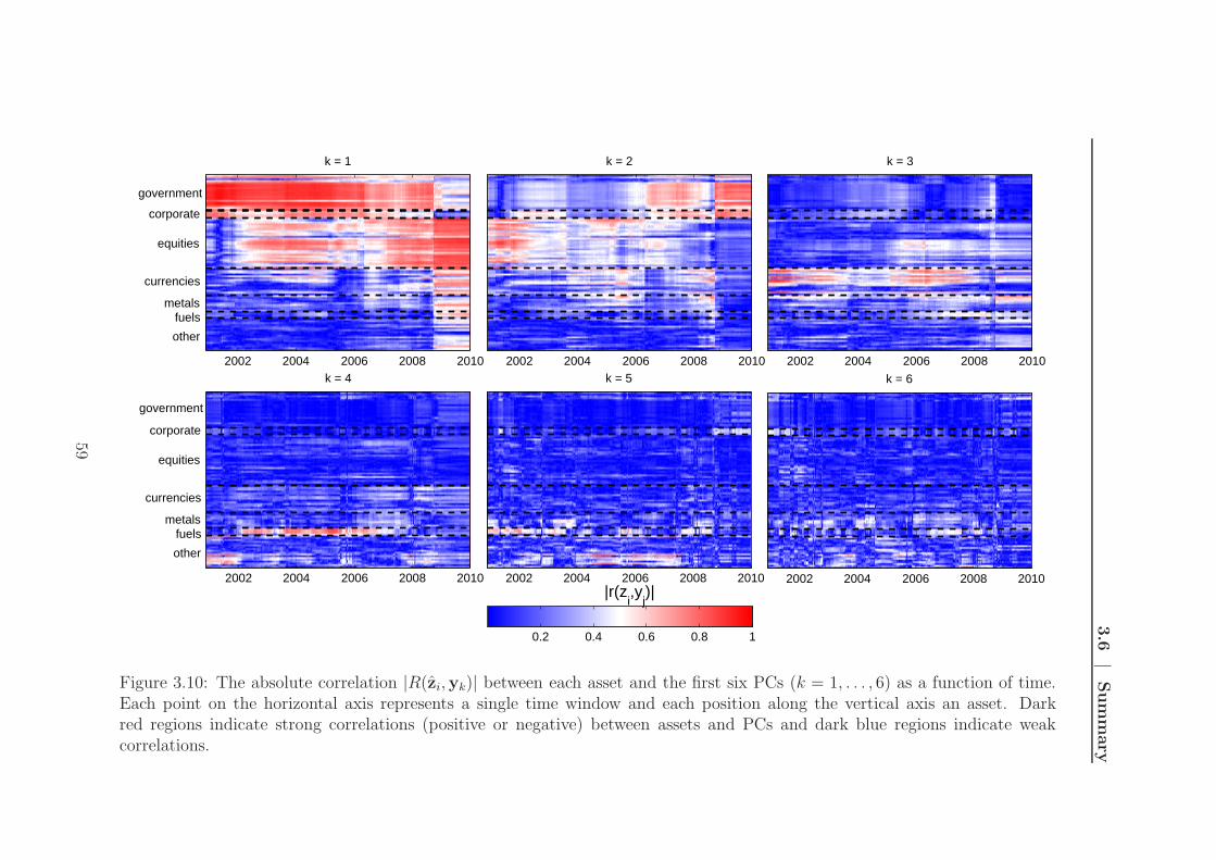
3.6
|Sum
mary
k = 1
2002 2004 2006 2008 2010
k = 3
2002 2004 2006 2008 2010k = 4
2002 2004 2006 2008 2010
k = 5
2002 2004 2006 2008 2010
k = 6
2002 2004 2006 2008 2010
k = 2
2002 2004 2006 2008 2010
0.2 0.4 0.6 0.8 1
corporate
equities
currencies
metalsfuels
other
corporate
currencies
metalsfuels
other
government
equities
government
|r(zi,y
j)|
Figure 3.10: The absolute correlation |R(zi,yk)| between each asset and the first six PCs (k = 1, . . . , 6) as a function of time.Each point on the horizontal axis represents a single time window and each position along the vertical axis an asset. Darkred regions indicate strong correlations (positive or negative) between assets and PCs and dark blue regions indicate weakcorrelations.
59

Chapter 3 | Financial Market PCA
increased from 2001–2010, with a sharp rise following the 2008 collapse of Lehman
Brothers. We further found that the number of significant components decreased and
the number of assets making significant contributions to the first PC increased over
this period. We investigated the evolving relationships between the different assets
by analyzing the correlations between the asset price times series and the first few
PCs. From 2001–2002, each of the first five components corresponded to a specific
market; however, after 2002 these relationships broke down and by 2010 nearly all of
the studied assets were significantly correlated with the first PC. The major changes
in the correlation structure following the collapse of Lehman shows the extent to
which market correlations increased during this crisis period.
60

Chapter 4
Community Structure in Networks
In this chapter, we describe several concepts that we will use in Chapters 5 and
6 in which we study network communities. We define a community, explain some
of the most widely used techniques for detecting communities in static networks,
discuss attempts to cluster networks using mesoscopic structures, and present a rel-
atively comprehensive review of the literature investigating communities in dynamic
networks.
4.1 Introduction
A network community consists of cohesive groups of nodes that are relatively densely
connected to each other but sparsely connected to other dense groups in the network.
Communities can represent functionally-important subnetworks [2, 75, 105, 107, 121,
139,243,244,295]. For example, a community in a cellular or genetic network might be
related to a functional module; a community in a stock market network might corre-
spond to stocks belonging to the same industrial sector; and a community in a social
network might correspond to a group of friends or a group of work colleagues. Com-
munities can affect dynamical processes (such as the spread of opinions and diseases)
that operate on networks [75, 107, 244], so their identification, and an understanding
of their structure, can potentially provide insights into these processes.
In this chapter we review some of the most widely used community detection
techniques. Because there is no rigorous definition of a community, different methods
often define communities in different ways; the main difference between methods is
essentially their precise definition of “relatively densely connected”. A vast amount
of research has been published on community detection in recent years, so this review
is not exhaustive. More detailed reviews of the community detection literature can be
found in Refs. [105,244]. However, these review articles focus on communities in static
61
Chapter 4 | Community Structure in Networks
networks (although there is a brief discussion of the dynamic communities literature
in Ref. [105]). In Chapter 5, we investigate dynamic communities and propose a
method for tracking communities through time; to illustrate how the methods we
present relate to other approaches, in Section 4.6 we review the dynamic communities
literature.
4.2 Notation
First, we introduce some of the notation that we use in the remainder of the thesis.
We consider undirected networks G = (V, E) that consist of a set of vertices V and
a set of edges E . We represent a network as an adjacency matrix A with elements
Aij . For unweighted networks Aij = 1 if an edge exists between nodes i and j and
is 0 otherwise; in weighted networks Aij can take other values (which are always
real numbers for the networks that we consider) that indicate the strength of the tie
between i and j.
We consider partitions P = C1, · · · , Cη of a network G into η disjoint communi-
ties C such that Ck ∩ Ck′
= ∅ and ∪ηk=1Ck = V, where |V| = N is the number of nodes
in the network. We use the letter C to identify a community and the scripted letter Cto represent the set of nodes in that community. We also reference the communities
in two different ways: Ck is the set of nodes in community k (k = 1, · · · , η), whereas
Ci is the set of nodes in the same community as node i (i = 1, · · · , N). We represent
the number of nodes in community k as |Ck| = nk.
4.3 Community detection methods
In statistics and data mining, there are a variety of methods for coarse graining data
to extract patterns and identify clusters of similar objects [84, 105]. Partitional clus-
tering techniques such as k-means clustering [84], multidimensional scaling [84], and
PCA1 have been successfully applied to problems from diverse disciplines. For exam-
ple, multidimensional scaling has been used to analyze voting patterns in the United
States Congress and the United Nations General Assembly (see Refs. [203, 241, 302]
and Chapter 6) and in Chapter 3 we use PCA to investigate correlations in financial
markets. Another widely used set of techniques are hierarchical clustering algorithms,
which can be split into two types: agglomerative and divisive. Agglomerative meth-
ods, such as linkage clustering, begin with a set of individual objects and iteratively
1See Chapter 3 for a detailed discussion of PCA
62

4.3 | Community detection methods
combine them based on their similarity [84].2 In contrast, divisive algorithms (which
include some spectral methods [221]) begin with all objects in a single cluster and
find smaller groups by iteratively splitting clusters.
Data clustering is closely linked to community detection. The widespread inter-
est of statistical physicists and applied mathematicians in community detection was
sparked by the 2002 publication of a paper by Girvan and Newman [121] in which they
proposed a technique for identifying communities using (geodesic) edge betweenness.
Betweenness [110] is widely used in social network analysis to quantify the extent
to which edges lie on paths that connect agents3. In the Girvan-Newman method,
edges with the largest betweenness are iteratively removed from the network. After
each edge removal the betweenness of the remaining edges is recalculated, which is
important because it can cause previously low-betweenness edges to have higher be-
tweenness. As the edges are removed the network breaks up into progressively smaller
isolated communities.
The main problem with the Girvan-Newman approach is that it tends to be slow
for large networks (unless they are very sparse) and typically produces poor results
for dense networks [244]. Nevertheless, Ref. [121] was the catalyst that led to the
explosion of research on community detection in networks and since its publication
many alternative community detection methods have been proposed. We explain
three of the more prominent methods below.
4.3.1 k-clique percolation
Communities are detected in k-clique percolation [234] using k-cliques, which are
complete subgraphs of k nodes that are connected with all k(k− 1)/2 possible edges.
The clique percolation method (CPM) is based on the idea that intra-community
edges are likely to form cliques as a result of their high density, but inter-community
edges are not. In Ref. [234], two k-cliques are described as adjacent if they share k−1
nodes; the union of adjacent k-cliques is called a k-clique chain; and two k-cliques
are considered to be connected if they are part of a k-clique chain. A community
is then defined as the union of a k-clique and all k-cliques that are connected to
it. By construction k-clique communities can share nodes, so the method allows
for the identification of overlapping communities. This is a useful property because
2We discuss linkage clustering in more detail in Chapter 5.3Note that the Girvan-Newman community detection method uses edge betweenness, but the be-
tweenness defined in Ref. [110] is the node betweenness [110]. In Chapter 5, we use node betweennessto study the roles of different exchange rates within the FX market.
63

Chapter 4 | Community Structure in Networks
many empirical networks possess overlapping communities. For example, in social
networks people often simultaneously belong to different communities consisting of
family, work colleagues, university friends, etc. The CPM has also been extended
to weighted networks [99]. The main problem with k-clique percolation is that the
community definition is very stringent and the rigid nature of the cliques means that
dense groups of nodes that are not quite as well connected as cliques are not identified
as communities.
4.3.2 Modularity maximization
Perhaps the most popular approach for detecting communities is a technique that
involves the maximization of a quality function known as modularity [224]. The iden-
tification of communities using graph modularity is based on the idea that random
networks are not expected to demonstrate community structure beyond small fluctu-
ations. Modularity therefore identifies communities by finding subsets of nodes that
are more strongly connected to each other than one would expect for a random null
model. We represent a network by an adjacency matrix A whose elements (edges)
Aij indicate how closely nodes i and j are related to each other. In this thesis, we
will only consider undirected networks, which implies that A is symmetric. If we let
P represent a partition of the n nodes in A into mutually disjoint communities, the
modularity Q of partition P is given by
Q(P) =1
2m
∑
ij
(Aij − Pij)δ(Ci, Cj) , (4.1)
where Ci is the community of node i and the null model Pij denotes the probability
that nodes i and j are connected for unweighted networks and the expected weight of
the link with which nodes i and j are connected for weighted networks. Modularity
is therefore easily extended from unweighted to weighted networks. The quantity m
represents the total number of edges in the network for unweighted networks and
the total edge weight for weighted networks and is given by m = 12
∑
i ki, where
ki =∑
j Aij is known as the degree of node i for unweighted networks and the strength
for weighted networks4.
Communities are identified by finding the partition P that maximizes Q. The
choice of null model is not entirely unconstrained because it is axiomatically the case
that Q = 0 when all of the nodes are placed in a single group.5 One is then restricted
4For an unweighted network a node’s strength is equal to its degree.5When all of the nodes in a network are in a single community, the number of edges within the
community and the expected number of such edges are both equal to m.
64

4.3 | Community detection methods
to null models in which the expected edge weight is equal to the actual edge weight
in the original network [220]. The simplest null model satisfying this criterion is a
uniform null model in which a fixed average edge weight occurs between nodes [244].
However, the strength distribution produced by this model is significantly different
to the distribution observed for many real-world networks. The most popular choice
of null model (introduced by Newman and Girvan [224]) is
Pij =kikj
2m, (4.2)
which preserves the strength distribution of the network and is closely related to the
configuration model [212].6
An important issue with using modularity as a quality function to identify com-
munities is that it suffers from a resolution limit [106]. Modularity optimization has
been shown to fail to find communities smaller than a threshold that depends on the
total size of the network and on the degree of interconnectedness between the network
communities. Communities smaller than the threshold tend to be merged into larger
communities, thereby missing important structures. However, many modularity-
maximization techniques can easily be adapted to other quality functions, and several
alternatives have been proposed that avoid the resolution limit by uncovering com-
munities at multiple resolutions, e.g., [17, 179, 220,254].
4.3.3 Potts method
In Ref. [254], Reichardt and Bornholdt proposed a multiresolution method in which
the network A is represented as an infinite-range, N -state Potts spin glass in which
each node is a spin, each edge is a pairwise interaction between spins, and each
community is a spin state. The Hamiltonian of this system is given by
H(λ) = −∑
ij
Jijδ(Ci, Cj) , (4.3)
where Ci is the state of spin i and Jij is the interaction energy between spins i and j.
The coupling strength Jij is given by Jij = Aij − λPij, where Pij again denotes the
expected weight of the link with which nodes i and j are connected in a null model
and λ is a resolution parameter. If Jij > 0 spins i and j interact ferromagnetically
6The difference between the two models is that the configuration model is conditioned on theactual degree (strength) distribution, whereas Newman and Girvan’s model is conditioned on theexpected degree (strength) distribution. In the configuration model, the probability of an edgefalling between nodes i and j is also given by Eq. 4.2 in the limit of large network size; however, forsmaller networks, there are corrections of order 1/N [220].
65

Chapter 4 | Community Structure in Networks
and seek to align in the same spin-state (join the same community); if Jij < 0
i and j interact antiferromagnetically and try to have different orientations (join
different communities). One can find communities by assigning each spin to a state
and minimizing the interaction energy of these states given by Eq. (4.3). Within
this framework, community identification is equivalent to finding the ground state
configuration of a spin glass.
Tuning λ allows one to find communities at different resolutions; as λ becomes
larger, there is a greater incentive for nodes to belong to smaller communities. The
Potts method therefore allows the investigation of communities below the resolution
limit of modularity. One can write a scaled energy Qs in terms of the Hamiltonian in
Eq. (4.3) as
Qs =−H(λ)
2m. (4.4)
The modularity is then the scaled energy with λ = 1. Community detection using
modularity optimization is therefore a special case of the Potts method.7 In this
thesis, we use the Potts method to detect communities and we employ the standard
model of random link assignment Pij = kikj/2m as the null model.
The number of possible community partitions grows rapidly with the number of
nodes [218], so it is typically computationally impossible to sample the energy space
by exhaustively enumerating all partitions [55]. A number of different heuristic pro-
cedures have been proposed to balance the quality of the identified optimal partition
with computational costs, e.g., [75, 107, 244]. In this thesis, we minimize Eq. (4.3)
at each resolution using the greedy algorithm of Ref. [44] which finds good quality
partitions and is computationally fast, so can be used to detect communities in large
networks. We note that quality functions like Eq. 4.3 have complex energy landscapes
and we are optimizing using an optimization heuristic, so care needs to be taken when
interpreting results for this method for real networks [128]. With this in mind, we
validate the results obtained using the greedy algorithm by reproducing the analysis
using spectral [221] and simulated annealing [141] algorithms.8
7Recently, an alternative version of the Potts method has been proposed that is able to deal withboth positive and negative links [294]. Even more recently, a new framework of network quality func-tions based on modularity has been proposed that can deal with time-evolving networks, networkswith multiple types of links, and multiple scales [214]; we discuss this method in Section 4.6.12
8See Ref. [105] for more details of these and other modularity (energy) optimization heuristics.
66

4.4 | Edge communities
4.4 Edge communities
All of the techniques that we have described thus far define communities as groups of
nodes. Recently, however, some community detection methods have been proposed
in which communities are defined as sets of edges [5, 6, 90]. Edge communities are
identified by considering line graphs [24]. A line graph is a representation of a network
in which the nodes represent edges in the original network and two nodes in the line
graph are connected if the corresponding edges in the original network are attached
to the same node. Identifying communities of nodes in line graphs is equivalent to
finding edge communities in the original network. In Ref. [90], Evans and Lambiotte
present methods for identifying communities in line graphs by maximizing quality
functions (derived from dynamical processes taking place on networks [177]) that are
similar to modularity (see Section 4.3.2).
4.5 Clustering networks
In Chapter 6, we introduce a framework for clustering networks based on comparing
their community structures at multiple resolutions. In this section, we review two
notable prior attempts to cluster networks using mesoscopic structures.
In Ref. [210], Milo et al. clustered a set of networks based on the frequency at
which certain small subgraphs they called motifs appeared in the networks. Motifs
represent small mesoscopic structures and some motifs can be considered as small
communities; for example, a 3-clique can be considered as a community because all
possible connections exist between the members of the motif. Milo et al. created pro-
files for each network indicating the over- or under-representation of motifs compared
to randomized networks with the same degree distribution and clustered the networks
based on these profiles. They studied 19 directed networks and 16 undirected net-
works and identified four families for each type of network. The directed families
included a family containing four gene transcription networks for microorganisms; a
family containing a network of signal-transduction interactions in mammalian cells,
two developmental transcription networks, and a network of synaptic wiring between
neurons; a family of three social networks and three world wide web (WWW) net-
works; and a family including four language networks and a model of a bipartite
network. The undirected network families consisted of a family containing a power
grid network and a “geometric model” network; a family containing another geomet-
ric model network and three protein structure networks; a family of six networks of
67

Chapter 4 | Community Structure in Networks
the internet at the level of autonomous systems; and the final family included four
Barabasi-Albert preferential attachment networks.
In Ref. [142], Guimera et al. clustered networks based on the over- or under-
representation of nodes with particular network roles. Guimera et al. first assigned
each node a role based on the node’s pattern of inter- and intra-community links and
then created profiles indicating the under or over-representation of node roles within
each network compared with randomized networks9. Based on these profiles, Guimera
et al. identified two clusters of networks. The first cluster included metabolic and
airport networks, and the second cluster included protein interaction and internet
networks. The authors hypothesized that the division of the networks into these
two clusters might result from the fact that the networks in the first cluster are
transportation networks, in which strong conservation laws must be obeyed, whereas
the networks in the second cluster could be considered as signalling networks, which do
not obey conservation laws. We discuss further the clustering in Refs. [210] and [142]
in Section 6.6.4.
4.6 Community dynamics
In comparison with the number of papers investigating communities in static net-
works, there are relatively few studies of communities in dynamic networks [105]. An
important reason for this comparatively small volume of work is the limited availabil-
ity of data sets for time-evolving networks. However, in recent years, time-evolving
data for large networks have become more widely available, in part because of the
rapid expansion of online social communities such as social networking sites and blog
communities. A desire to understand the evolution of these communities has led to
more researchers (particularly computer scientists) studying dynamic networks and
trying to answer some of the fundamental questions on community dynamics. These
include: how do communities change over time; what community properties result in
stable communities; and what features of a community determine whether an individ-
ual will join (or leave) that community? These questions are key to understanding the
evolution of many systems: for example, the evolution of groups of employees within
large organizations can provide insights into the organization’s global decision-making
behaviour; an understanding of the dynamics of sub-populations of people can help
develop strategies for preventing the spread of diseases [23]; and an understanding of
9Guimera et al. considered two different ensembles of random networks. In the first ensemble,they preserved only the degree distribution of the original network; in the second ensemble, theypreserved both the degree distribution and the modular structure of each network.
68

4.6 | Community dynamics
the changes in correlations between groups of financial assets can lead to better risk
management tools.
Although the study of dynamic communities is still in its infancy, several methods
have been proposed for detecting and tracking communities in dynamic networks. In
the remainder of this chapter, we describe the different techniques.
4.6.1 Early studies
In an early study of community dynamics, Toyoda and Kitsuregawa investigated the
evolution of communities of web pages [290–293]. They first proposed a method to
identify web page communities in static networks [290] using a modified version of the
Companion algorithm proposed by Dean and Henzinger [78]. Companion finds web
pages related to a particular URL by only exploiting the hyperlink-structure of the
web; i.e., it does not use information about the content or usage levels of web pages.
By following links from seed pages, the algorithm identifies web pages related to the
seed page and considers seed pages to belong to the same community if they are related
to similar sets of pages. In Refs. [291, 292], Toyoda and Kitsuregawa extended this
work to track web communities through time. They mapped communities between
consecutive time steps based on the overlap of nodes (i.e., URLs) and defined the
descendant of a community C(t) as the community C(t + 1) that shared the most
nodes with C(t); if more than one community at t + 1 shared the same number of
nodes with C(t), they selected the community with the largest number of nodes as
the descendant.
Toyoda and Kitsuregawa defined six types of community changes between consec-
utive time steps: emerge (a community C(t+1) emerged if it did not share any nodes
with any of the communities in the network at time t), dissolve (a community C(t)
dissolved if it did not share any nodes with any of the communities in the network at
t+1), grow, shrink, split, and merge. A community C(t) was only considered to grow
or shrink if it shared all of its nodes with one community at t + 1; i.e., a community
grew if the nodes that joined it were new to the network and a community shrunk if
the nodes leaving it disappeared from the network. If a community C(t+1) contained
nodes from more than one community at time t, it was considered to have merged;
similarly, if more than one community at t + 1 contained nodes from a community
C(t), then C(t) was considered to have split.
Based on these events, Toyoda and Kitsuregawa defined several quantities for
describing community evolution, including a growth rate; a stability index; indices
for measuring the rate at which nodes appeared in (disappeared from) communities;
69

Chapter 4 | Community Structure in Networks
and indices for measuring the rate at which split and merge events occurred. They
applied this framework to an evolving sequence of networks of Japanese web archives
for each of the years 1999–2002 and found that changes in the community structure
were largely a result of merge and split events. This observation seems unsurprising
given the tight constraints on nodes’ community membership for the other types of
event. They also found that the distribution of community sizes and the distributions
of the sizes of emerged and dissolved communities followed power laws.
In another early study [152], Hopcroft et al. employed a very different approach
to study the evolution of weighted citation networks10 in which the nodes represented
papers and the weights were given by the cosine similarity [84] between vectors rep-
resenting each paper’s citations. Hopcroft et al. identified communities using ag-
glomerative hierarchical clustering, but found that the clusters were very sensitive to
random perturbations in the network. This led them to define “natural communi-
ties” as clusters that were robust to the random removal of nodes. To identify natural
communities, Hopcroft et al. created n realizations of the network in which 5% of the
nodes were randomly removed and compared clusters C in the original network with
clusters C ′ in the perturbed networks using the similarity function
min
( |C ∩ C′||C| ,
|C ∩ C′||C′|
)
, (4.5)
where |C ∩C′| indicates the cardinality of the intersection of nodes in the two clusters.
They defined a natural community as a cluster in the original network whose similarity
with any cluster in a perturbed network exceeded a pre-defined threshold p for a
fraction f of the networks with nodes removed.11
Hopcroft et al. tested their method by comparing citation data for the years
1990–1998 with data for 1990–2001, which enabled them to identify changes that
occurred in the community structure during the period 1999–2001. They associated
each community with a research topic by considering the most frequent words in the
titles of the papers in the communities. They then classified the natural communities
in the second period as either established or emerging depending on their overlap with
communities in the first period. They found that some of the established communities
grew rapidly while others stagnated, and that some of the communities that emerged
had split from communities that existed in the first period. Based on the evolution
10The citation data covered the period 1990–2001 and was downloaded from the CiteSeer database,which is available at http://citeseer.ist.psu.edu/.
11Hopcroft et al. created n = 45 networks in which 5% of nodes were removed and set f = 0.6;they set p = 0.7 for clusters containing fewer than 1,000 papers and p = 0.5 for larger clusters.
70

4.6 | Community dynamics
of the different communities, they identified new, expanding, and declining fields of
research.
An important issue with the approach proposed by Hopcroft et al. is that hier-
archical trees contain clusters at several different levels and their method does not
identify the level at which the clusters are most appropriate. In addition, there
are several parameters that the user must define, including the fraction of nodes to
randomly remove from the original network to create the comparison networks; the
overlap threshold p for a pair of clusters to be considered similar; and the fraction of
perturbed networks f in which a cluster needs to match another cluster for it to be
considered a natural community. The node compositions of the natural communities
depend on all of these parameters.
4.6.2 Comparing and mapping communities
In Ref. [152], Hopcroft et al. used the similarity function defined in Eq. 4.5 to com-
pare communities, but there are several other functions that can be used (some of
which we describe later in this chapter). For many of the methods that compare
communities using a similarity function, it is also necessary to select an appropriate
overlap threshold that the similarity function must exceed for two clusters to be con-
sidered similar (the parameter p in Hopcroft et al.’s study). In most studies a formal
procedure is not defined for selecting the threshold; instead this parameter is chosen
using ad hoc methods or is simply set to a value that is found a posteriori to produce
meaningful results.
Perhaps the most important issue with methods that identify descendent commu-
nities based on maximum node (or edge) overlap is that they can lead to equivocal
mappings following splits and mergers. For example, consider a community Cf(t) that
splits into two communities Cg(t + 1) and Ch(t + 1). If the overlap between Cf(t)
and Cg(t + 1) is identical to the overlap between Cf (t) and Ch(t + 1) then it is not
obvious which community represents the descendent of Cf (t). For the specific case
of two communities with identical node overlaps with a community at the previous
time step, Toyoda and Kitsuregawa [291,292] chose the descendant as the community
containing the largest number of nodes. However, there are other plausible choices.
For example, a tie in node overlap could be broken by selecting the community with
the highest edge overlap as the descendant.
This highlights the more general question of whether communities should be
mapped based on node or edge overlap. For example, consider a community Cr(t) that
splits into two communities Cs(t+1) and Ct(t+1), such that Cs(t+1) has a greater
71

Chapter 4 | Community Structure in Networks
node overlap with Cr(t), but Ct(t + 1) has a greater link weight in common with
Cr(t). In this case, either community could be identified as the descendant of Cr(t)
depending on whether one considers node or edge overlap to be a more important
measure of community similarity. Most methods that we describe map communities
based on node overlap; in practice, the choice between node or edge overlap is likely
to depend on which measure is most appropriate for a particular analysis.
4.6.3 Dynamics of known partitions
Although in most work on community dynamics methods are presented both for
community detection and community tracking, in some studies the communities are
already known. In Ref. [23], Backstrom et al. investigated the evolution of com-
munities of bloggers on the LiveJournal blogging website12 and communities within
a co-authorship network of computer scientists taken from the Digital Bibliography
and Library Project (DBLP) website13. Backstrom et al. did not detect communities,
but instead studied the evolution of known groups. In the case of LiveJournal the
communities corresponded to blogging groups that the users joined; for the DBLP
network, conferences were used as proxies for communities.
For both data sets, Backstrom et al. found that the probability of a person joining
a community increased with the number of people that they knew in the community,
but that there was a “diminishing return” property in which this probability rose
at an increasingly slower rate as the number of friends already in the community
increased. For the LiveJournal network, they also showed that an individual was
more likely to join a community if the people that they knew in the community
already knew each other, but that groups with a very large number of 3-cliques
grew less quickly than groups with relatively few such cliques. These results imply
that the tendency of an individual to join a community is not just influenced by the
number of friends that individual has within the community, but crucially also by how
those friends are connected to each other. Backstrom et al. hypothesized that the
slower rate of growth of communities containing large numbers of 3-cliques could be
because such “cliquishness” makes communities less attractive to join; alternatively,
they suggested that many 3-cliques could indicate a community that has stopped
gaining new members, but continues to gain new edges between existing members.
Finding an explanation for this observation is an interesting open question because of
12See http://www.livejournal.com/.13DBLP is a database of bibliographic information for computer science journals. See http:
//www.informatik.uni-trier.de/~ley/db/.
72

4.6 | Community dynamics
its implications for the potential rate of growth of online communities such as social
networking websites.
Berger-Wolf and collaborators have proposed several different methods for study-
ing dynamic communities [35]. In Ref. [36], Berger-Wolf and Saia presented a tech-
nique in which it was assumed that the community partition at each time step was
already known. They created a network of these known communities in which two
communities C and C ′ were linked if the similarity
2|C ∩ C′||C| + |C′| (4.6)
exceeded a pre-defined threshold βm. Within this framework two communities could
be connected irrespective of the number of time steps separating the networks in which
they were observed. This is in contrast to other techniques that create networks of
communities but only allow communities to be connected if they appear in networks
separated by a specified number of time steps (e.g., Refs. [91, 93, 96, 97] which we
discuss in Section 4.6.6.).
Using the network of communities, Berger-Wolf and Saia then defined a metagroup
as any connected group of at least αm communities and considered that an individual
node was a member of a metagroup if it belonged to more than γm communities in
that metagroup. They then defined the most persistent metagroup as the metagroup
that contained the most communities; the most stable metagroup as the metagroup
that contained the most links as a fraction of the number of time steps over which
the group persisted; and the largest metagroup as the metagroup that contained the
most nodes.
Berger-Wolf and Saia tested the metagroup framework on the southern women
social network [76], which is a standard benchmark in social network analysis [112].
The southern women data set consists of details of the participation of 18 women
in 14 social events in Mississippi in the 1930s; the network contains 14 communities
corresponding to the groups of women that attended each of the 14 events. Berger-
Wolf and Saia found good agreement between the membership of the most stable
metagroups and the clusters identified in previous studies of the same data. They also
considered the importance of communities and nodes to the existence of metagroups
at different similarity thresholds βm and length thresholds αm and found that the
metagroups were robust to the removal of particular communities and individuals
from the population. Such observations are of practical interest in epidemiology; for
example, targeted vaccination of individuals whose removal results in the break-up of
metagroups might help to prevent the spread of diseases [10,62, 151].
73

Chapter 4 | Community Structure in Networks
4.6.4 Dynamic subgraphs and cliques
There are several studies of dynamic networks in which motifs consisting of repeated
subgraphs, such as cliques, are investigated. As we discussed in Section 4.3.1, a
k-clique in an unweighted network is a set of k nodes that are connected with all
k(k− 1)/2 possible edges, so they represent particularly strong relationships between
a group of nodes. Motifs need not contain all possible links between nodes, but
if a subgraph appears regularly through time it indicates a persistent or recurrent
relationship between a group of nodes.
In Ref. [175], Lahiri and Berger-Wolf defined frequent and periodic subgraphs
as groups of nodes that had the same intra-group links for more than a pre-defined
fraction of observed time steps, and groups of nodes that had the same relationships in
networks separated by a constant number of time steps, respectively. For example, a
3-clique that appeared every fifth time step was considered to be a periodic subgraph.
Lahiri and Berger-Wolf investigated subgraph dynamics for a social network of zebras
[283], a network of e-mail exchanges within Enron14, a co-appearance network for
celebrities in photos on the Internet Movie Database (IMDB)15, and a contact network
of mobile phone users at MIT [85]16. Lahiri and Berger-Wolf identified many frequent
and periodic subgraphs for each of these data sets, including a periodic subgraph of
actresses from the television show Desperate Housewives in the IMDB network. This
subgraph had a period of 364 days and is likely to result from the joint appearance
of these actresses at annual awards shows.
In Ref. [311], Yoneki et al. also studied the MIT contact network data set as well
as three other dynamic contact networks. Yoneki et al. focused on the distribution of
the durations of meetings between particular groups and the distribution of the times
between these meetings. They took a stricter approach than Lahiri and Berger-Wolf
[175] by only investigating cliques – this meant that every node in the studied groups
had to be connected to every other node. They analyzed k-cliques with k = 3, · · · , 8nodes and found that the durations of meeting times for the cliques were power-law
distributed, but the intervals between these meetings were not.
In another study of dynamic motifs [157], Jin et al. investigated the evolution
of weighted subgraphs. They analyzed networks in which there was a time series
associated with each node and the edge weights were a function of the time-dependent
14The data for the Enron e-mail network is available at https://www.cs.cmu.edu/~enron/.15See http://www.imdb.com/.16The contact networks were constructed using mobile phones fitted with proximity tracking
technology that recorded when two individuals were located near to each other.
74

4.6 | Community dynamics
pairwise correlations between these time series. Community detection in networks of
this kind is equivalent to the problem of clustering multivariate time series [187]. Jin
et al. defined a trend motif as any subgraphs whose edge (or node) weights consistently
increased (or decreased) by more than a threshold amount over a specified time period.
They investigated a network of trade between countries, in which the node weights
represented each country’s share of global gross domestic product (GDP) [122], a
stock market network [230], and a protein interaction network [27, 278], and found
several examples of trend motifs in each case. For example, they identified a subgraph
in the trade network over the period 1980–1990 containing the U.K., Japan, and the
U.S. in which each country’s share of global GDP was trending upwards. In another
subgraph for the period 1981–1989 containing the U.S., Mexico, Argentina, and South
Africa, the U.S.’s share of global GDP was trending upwards while the share of each
of the other countries was trending downwards.
Jdidia et al. [154] also identified stable cliques in an evolving co-authorship network
for the Infocom conference on computer communications over the period 1985–2007.
They investigated cliques with three of more nodes and considered a clique to be
stable if it appeared in three or more networks. Using this approach, they identified
many stable cliques of collaborators based on their conference publications.
In the same paper, Jdidia et al. also proposed a method for detecting communities
in dynamic networks based on the behaviour of random walkers.17 They first created
an aggregate network consisting of a combination of the networks for individual time
steps coupled through additional links. They introduced two types of links between
consecutive networks: (1) a node in a network at time t was connected to itself if it
also appeared at t + 1, i.e., a link was added between node i at time step t and node
i at time step t + 1; (2) a link was added between node i at time step t and node j
at t + 1 if there existed a node k such that i and k were linked at time step t and j
and k were linked at t + 1; these edges were called transversal edges.
Jdidia et al. detected communities in this network by maximizing modularity us-
ing a variant of the walktrap algorithm proposed by Pons and Latapy [240]. This
algorithm identifies communities based on the observation that random walkers on a
graph tend to get “trapped” in densely connected parts of the graph that correspond
to communities. Jdidia et al. presented an example of an evolving community of
collaborators in which a stable clique of researchers gained and lost additional collab-
orators through time. They also investigated the probability of an author joining the
conference program committee board as a function of the number of their co-authors
17We describe other methods based on random walkers in Section 4.6.8.
75

Chapter 4 | Community Structure in Networks
already on the board and found that the probability of an author joining the com-
mittee increased with the number of their co-authors already on it. This result is
consistent with Backstrom et al.’s [23] observation that the probability of a person
joining a community increases with the number of people that they know in that
community.
4.6.5 Dynamic clique percolation
All of the studies that we described in Section 4.6.4 uncovered recurrent relationships
between groups of nodes by detecting frequent subgraphs and cliques. The CPM
method described in Section 4.3.1 extends the idea of cliques by defining communities
as groups of overlapping cliques. This method is based on the observation that intra-
community edges are likely to form cliques as a result of their high density, but inter-
community edges are not. In Ref. [233], Palla et al. extended the CPM framework to
investigate community dynamics.
As we discussed in Section 4.3.1, communities detected using CPM can overlap
(i.e., share nodes), which can lead to additional problems when trying to identify
community descendants using node overlap. For example, consider the situation
in which a community C(t) increases in size between time steps t and t + 1 and the
resulting community C(t+1) overlaps with another community C ′(t+1). The overlap
between C(t + 1) and C ′(t) might be larger than the overlap between C(t + 1) and
C(t) resulting in C(t + 1) being identified as the descendant of C ′(t) and not C(t).
Palla et al. tackled this problem by considering the graph G(t, t +1), which consisted
of the union of nodes and edges from the two graphs G(t) and G(t+1). The rationale
for this approach is as follows. Let P(t) denote the set of communities from graph
G(t), P(t + 1) the set of communities from graph G(t + 1), and P(t, t + 1) the set of
communities identified for the combined graph G(t, t+1). For any community in P(t)
or P(t+1) there is exactly one community in P(t, t+1) containing it, which is found
by comparing edges. The descendant of C(t) is then the community contained in the
same community C(t, t + 1) as C(t) with which C(t) has the largest edge overlap.
Palla et al. applied this method to a call network of mobile phone users and to
a co-authorship network of condensed matter physicists. For both networks, they
found that the age of a community was positively correlated with its size (i.e., older
communities tended to be larger on average) and also found that the membership of
large communities varied more than small communities, which tended to be almost
static. They further found that communities whose members had relatively strong
connections with nodes outside their community were more likely to break up, and
76

4.6 | Community dynamics
that nodes that were only loosely connected to their community were more likely
to leave that community than nodes with strong intra-community connections. The
observation that nodes are more likely to leave a community if they are only weakly
connected to that community is complementary to the observation made by Back-
strom et al. [23] and Jdidia et al. [154] that the probability of an individual joining a
community increases with the number of people they know in that community.
Reference [233] provides answers to several of the fundamental questions relating
to community dynamics, but the results should be validated using other techniques.
This is important because there are some issues with the CPM method; for example,
there are several possible choices for the clique size; and the definition of a community
is very stringent (see Section 4.3.1). It would also be interesting to investigate if
similar results are observed for other types of network.
4.6.6 Edge betweenness methods
In contrast to the motif-based methods described in Sections 4.6.4 and 4.6.5, edge
betweenness methods do not require the user to specify the structures to identify.
In Ref. [92], Falkowski et al. investigated community dynamics using the Girvan-
Newman edge betweenness method (see Section 4.3) and a method proposed by
Radicchi et al. [247]. The Radicchi method is similar to the Girvan-Newman method
but, instead of iteratively removing edges with the lowest betweenness centrality,
edges with the lowest edge-clustering coefficient are removed. The edge-clustering
coefficient is analogous to the the node-clustering coefficient [305] and is defined as
the number of 3-cliques to which an edge belongs divided by the total number of
3-cliques the edge could potentially belong to based on the degrees of the nodes it
connects. The basic idea is that edges with a low edge-clustering coefficient belong
to fewer small cliques than edges with high edge-clustering coefficient, so these edges
are considered to be more likely to run between communities.
To create dynamic networks, Falkowski et al. split their network data into time
periods and constructed a network for the interactions within each period.18 Falkowski
et al. mapped communities between consecutive time steps based on the percentage
node overlap exceeding a threshold and defined several community events: persists,
disappears, merges, and splits. They further divided the persist events into grows and
declines transitions. A community grew if the number of members increased between
18This is in contrast to other studies, such as the work of Hopcroft et al. [152], in which communitydynamics were investigated by cumulatively adding data to a network and identifying changes inthe aggregated network.
77

Chapter 4 | Community Structure in Networks
time steps; a community declined if the number of members decreased and/or the
number of edges, or the edge weights, decreased between time steps. In contrast to
the grow and shrink events defined by Toyoda and Kitsuregawa in Refs. [291, 292],
the grow and decline events defined by Falkowski et al. allowed nodes to join from
existing communities, or leave to join other communities; i.e., the nodes joining a
community did not have to be nodes not previously in the network and the nodes
leaving a community were not required to be nodes leaving the network. Falkowski
et al. also introduced software for visualizing community dynamics in Ref. [92], but
they did not provide details of any results found using their method.
Falkowski et al. extended the work of Ref. [92] in a series of papers [91,93,96,97] in
which they matched two communities C and C ′ at different time steps if the overlap
function|C ∩ C′|
min(|C|, |C′|) (4.7)
exceeded a threshold ρm. Instead of simply comparing communities at consecutive
time steps, they matched communities between all networks within τp time steps
of each other. They then constructed a graph in which each community observed
over the full evolution of the network represented a node and they connected all
nodes that appeared in networks within τp time steps of each other for which the
community overlap exceeded ρm. Finally, they found groups of similar communities in
this network of communities using the Girvan-Newman edge betweenness algorithm.
An issue with this method is that it suffers from two of the weaknesses that we
described in Section 4.6.2; namely that the user is required to select values for the
parameters ρm and τp and the detected communities are sensitive to these choices.
Using this method to track dynamic communities, in Ref. [97] Falkowski et al.
defined several quantities that described the relationships between nodes and their
communities. These included the involvement of a node, which measured the number
of intra-community interactions of nodes at a single time step; the participation, which
measured the involvement of nodes in a particular community over all time steps as
a fraction of the total interactions of the node; and the relevance, which measured
the involvement of nodes in a community as a fraction of the total interactions over a
specified period. Falkowski et al. used this framework to perform a “preliminary set
of proof-of-concept experiments” on a social network.19
19Although the network is not specified in Ref. [97], this paper extends the work presented inRef. [93] in which an online social network of students from the University of Magdeburg is studied,so it seems likely that this network is also used in Ref. [97].
78

4.6 | Community dynamics
4.6.7 Density methods
Other authors have proposed techniques for detecting communities based on the den-
sity of nodes in different regions of the network, where the precise definition of density
depends on the method. In Refs. [94, 95], Falkowski et al. proposed a density-based
method for detecting communities in graphs that are growing both in terms of the
number of nodes and the number of edges. They assigned nodes to the same cluster
if they were density connected ; nodes were described as density connected if their was
some overlap in their neighbourhoods, where a node’s neighbourhood was all nodes
on the graph within a specified distance. Dense regions of the graph therefore had
many nodes within a small distance of each other.
Falkowski et al. designed this approach with the analysis of graphs that evolve
incrementally (i.e., only a few nodes join or disappear from the network at a time)
in mind because the insertion (or deletion) of nodes was only considered to affect
the clustering in the neighbourhood of the inserted (deleted) nodes. Because of this
property, this method is potentially useful for uncovering the changes in communities
in networks constructed from generative models involving attachment mechanisms in
which new nodes are iteratively added to the network. Falkowski et al. applied this
technique to the Enron e-mail network and compared the communities with those
obtained using the edge betweenness method discussed in Section. 4.6.6. They found
that the density-based algorithm tended to detect small dense communities whereas
the edge betweenness method often merged small groups. This highlights that differ-
ent community detection methods often identify different communities. These differ-
ences are important because they can affect the conclusions regarding the properties of
dynamic communities. Given this, the most rigorous approach that is currently avail-
able to assess the reliability of the outputs of different dynamic community techniques
is only to consider features that are similar across multiple methods as meaningful.
In Ref. [126], Goldberg et al. proposed another density-based method and used it
to investigate the dynamics of a directed network of blogs from the Russian section
of LiveJournal. They first constructed networks of bloggers in which each node rep-
resented a blogger and there was a directed edge from the author of any comment to
the author of the blog where the comment was posted. They then investigated the
evolution of several microscopic (e.g., mean clustering coefficient) and macroscopic
(e.g., the fraction of nodes in the largest connected component) properties of the
network as well as the community dynamics.
Goldberg et al. defined a community C as a set of nodes C for which for every
node i ∈ C (resp. i /∈ C), removing i from C (resp. adding i to C) resulted in a
79

Chapter 4 | Community Structure in Networks
community C with a smaller value of a “density function” Ψ(C) given by
Ψ(C) =win
win + wout
+ µ2win
|C|(|C| − 1), (4.8)
where win is the number of edges connecting two nodes in C, wout is the number of
edges with only one end connected to a node in C, and µ is a user-defined parameter.
Goldberg et al. then considered a community C(t + 1) to be the descendant of a
community C(t) if the similarity function
|C(t) ∩ C(t + 1)||C(t) ∪ C(t + 1)| (4.9)
exceeded a threshold αt, which they set to 1/3 because it was found to produce
meaningful results. They discovered that the number of blogger communities that
persisted for more than a few weeks was very small, which is unsurprising given that
they also observed that 25% of the nodes changed between some time steps. However,
the persistence of communities determined using this method is affected by the value
of the threshold αt, so the results might have been different for other values of this
parameter. The dependence of the results on αt highlights why it can be undesirable
for dynamic community detection methods to incorporate user-defined parameters.
4.6.8 Random walkers
In Section 4.6.4, we described a dynamic community detection algorithm that iden-
tifies communities using random walkers [154]; several other methods have been pro-
posed that investigate community dynamics using similar techniques.
In Ref. [22], Asur et al. investigated the evolving relationships between nodes
and communities. They detected communities at each time step using the Markov
cluster algorithm introduced by van Dongen [300] and defined five types of community
evolution events: continue (the community contained the same nodes at consecutive
time steps, but not necessarily the same edges), κ-merge (two communities merged if
a community existed at the next time step that included more than κ% of the nodes
belonging to the two communities), κ-split (a community split if more than κ% of
nodes were in different communities at the next time step), form (no pair of nodes in
a community C(t + 1) were in the same community at t), dissolve (no pair of nodes
in a community C(t) were in the same community at t + 1). The final two events are
equivalent to the emerge and dissolve events defined by Toyoda and Kitsuregawa in
Refs. [291, 292].
80

4.6 | Community dynamics
Asur et al. also defined four types of events involving nodes: appear (a node joined
the network), disappear (a node left the network), join (a node joined a community),
and leave (a node left a community). Based on these events, they defined four indices
that measured the behaviour of the nodes in relation to the communities: the stability
index (the tendency of a node to interact with the same nodes over time), the socia-
bility index (the number of different interactions in which a node was involved), the
popularity index (the number of nodes attracted by a community in a time interval),
and the influence index (the number of nodes that left or joined a community at the
same time as a node).
Asur et al. used these measures to describe the community evolution of a co-
authorship network taken from DBLP database and a network of clinical drug trial
patients in which the weights of the edges were based on the correlation in patients’
liver toxicity levels during the trial. For the drug network, they identified several
patients with a low stability index and suggested that this implied that these patients
were suffering from side effects from the drugs. The reasoning behind this suggestion
was that patients with a low stability index regularly switched between communities
because of large variations in their response to the trial drugs, and these variations
implied that they were responding badly to the treatment. Asur et al. also used the
influence index to predict the appearance of links within clusters.
In another method utilizing random walkers, Lin et al. [190] proposed a technique
that identified communities by finding the partition of the network that minimized
the number of steps that the walkers needed to take to reach other nodes within
the same community and maximized the number of steps required to move between
communities. In contrast to many of the methods that we discuss, instead of mapping
communities between time steps based on node or edge overlap, Lin et al. compared
vectors representing the interactions between members of a community at different
time steps. They then defined five types of community evolution: one-to-one mapping,
merge, split, extinct, and emerge. Each of these events corresponds to one of the five
events defined in Ref. [22] by Asur et al.
Lin et al. tested their method on a blog network in which each node represented
a blogger and there was a directed edge from the author of any comment to the
author of the blog where the comment was posted. Based on this network, they then
constructed weighted networks for several different search queries in which the edge
weights in a network for a particular query were based on the relevancy of a post to
that query. For example, they studied the community evolution in a network based on
the query “London bombing” and found that there were initially two distinct political
81

Chapter 4 | Community Structure in Networks
blog communities, with different political interests, which joined together when their
interests converged – in this case, when both communities began to discuss terrorist-
related issues, such as the investigation of terrorist suspects.
The major weakness of the method proposed by Lin et al. which is common to sev-
eral of the methods that we discuss, is that the user is required to input the number of
communities to identify at each time step. In almost all situations, it is desirable that
the appropriate number of communities is determined by the community-detection
algorithm from the structure of the data, rather than being specified by the user.
Random walkers have also been used to investigate communities in dynamic net-
works using methods based on modularity maximization (see Section 4.3.2). In
Ref. [177], Lambiotte et al. demonstrated the equivalence of modularity-like qual-
ity functions and Laplacian dynamics of populations of random walkers. Recently,
Mucha et al. extended this framework to study the community structure of multislice
networks, which are combinations of individual networks coupled through additional
links that connect each node in one network slice to itself in other slices [214].20
Their generalization includes an additional parameter that controls the strength of
the coupling between slices. The different connections between the network slices
are flexible and can represent connections between time slices, connections between
networks including different types of links, or connections across different resolutions.
The method allows one to simultaneously identify communities at different time steps
and to systematically track the development of communities through time.
Mucha et al. tested their method on an evolving roll call voting network for the
U.S. Senate over the period 1789–2008 (see Refs. [241, 306] and Chapter 6). They
uncovered details about the group voting dynamics of U.S. Senators that would not be
captured by simply considering the union of the partitions for the different networks.
In particular, their analysis identified several important changes in U.S. politics, such
as the formation of political parties and the beginning of the Civil War. The method
proposed by Mucha et al. is particularly appealing because it can simultaneously deal
with multiple time steps, multiple types of edge, and multiple resolutions. However,
the user is again required to make a parameter choice; in this case to choose an
appropriate value for the parameter controlling the coupling between different network
slices.
20This approach bears similarities to the method proposed by Jdidia et al. in Ref. [154] (seeSection 4.6.4).
82

4.6 | Community dynamics
4.6.9 Graph colouring
The investigation of community dynamics has also been cast as a graph colouring
problem. In Ref. [286], Tantipathananandh et al. defined a method for investigating
community dynamics in which the colour of a node at a time step represented the
node’s community affiliation. To derive an optimization formulation for the commu-
nity detection problem, they made three explicit assumptions about the behaviour of
nodes: (1) a node tends not to change its community affiliation very frequently (i.e.,
a node does not change colour very often); (2) if a node does change its community
affiliation (colour), it will usually move between only a few communities; (3) nodes in
the same community interact more than nodes in different communities. They then
assigned costs to penalize deviations from each of these behaviours and defined an
optimization problem in which the community affiliation was determined by minimiz-
ing the sum of these costs; they also assigned parameters to each of these costs that
could be tuned by the user to adjust the relative importance of assumptions (1)–(3).
The resulting optimization problem is NP-hard, so in Ref. [286] Tantipathananandh
et al. proposed several computational heuristics to identify approximate solutions and
they presented further heuristics in Ref. [285].
Tantipathananandh et al. tested this framework on the southern women’s data
set [76] and on a social network of zebras [283] and found good agreement between the
communities they identified and the communities found in prior studies. However,
clearly the assumptions about node and community behaviour used to define the
graph colouring problem are very strong and in general they are not valid for other
networks.
4.6.10 Graph segmentation and change points
In several of the studies we have discussed, events have been defined to describe
changes in individual communities (e.g., merge and split events). In this section,
we describe two methods that identify time steps at which the overall community
partition of a network changed.
In Ref. [282], Sun et al. investigated dynamic communities in bipartite networks
using methods of information compression. Instead of identifying communities in the
network for each time step independently and then comparing communities across
time steps, Sun et al. separated the sequence of networks into segments such that
the optimal community partitions of the networks in each segment were similar. The
83

Chapter 4 | Community Structure in Networks
networks in a segment were then considered to represent the same stage of the evo-
lution of the network and were characterized by the same partition of the nodes into
communities. Furthermore, the boundaries between segments were considered to cor-
respond to “change points” in the evolution of the network. Sun et al. determined
the partitions of the sequence of networks into segments and of the segments into
communities using the minimum description length principle [136, 257], which is a
formalization of Occam’s Razor [80] in which the best description of a data set is the
one that results in the largest compression of the data. They calculated an encoding
cost for the description of the communities in each segment and summed this value
over all segments to give a total encoding cost for the sequence of networks. The
optimal partition of the sequence of networks into segments and of the segments into
communities was the partition that minimized the total encoding cost. Sun et al.
applied this technique to several data sets, including the Enron e-mail network, for
which they identified a change point at the time when the investigation into document
shredding at the company began and the CEO resigned.
Duan et al. used a different approach to partition evolving, directed, weighted
networks into segments in which all of the networks had similar optimal partitions
into communities [83]. They began by partitioning the first two instances G(t = 1) and
G(t = 2) of the network into community partitions P(1) and P(2), respectively, by
maximizing modularity for each network.21 They compared the two partitions P(1)
and P(2) using a similarity function based on the intersection of the communities at
the two time steps. They then proceeded in different ways depending on the value of
this similarity:
1. If the similarity exceeded a pre-defined threshold, the two networks were consid-
ered to belong to the same segment. Duan et al. then constructed an aggregate
network G(1, 2), containing all of the nodes and the total edge weight in G(1),
and G(2) and identified communities in this new network. They compared the
community partition P(3) of the third network G(3) with the partition for the
aggregate network G(1, 2) to determine if this network was sufficiently similar to
also join the segment. If it was, they integrated G(3) into the aggregate graph
G(1, 2); if it was not, there was a change point and G(3) began a new segment.
2. If the similarity of the first two partitions P(1) and P(2) did not exceed the
threshold, they were considered to belong to different segments, so there was a
21See Ref. [184] for details of the generalization of modularity to directed networks.
84

4.6 | Community dynamics
change point between time steps 1 and 2 and the community partition P(3) of
the third network was then only compared to the second partition P(2).
They repeated this process for each of the time steps of the evolving network. Duan
et al. also applied their method to the Enron e-mail network and identified stable and
fluctuating periods during which there were few and many changes points, respec-
tively.
4.6.11 Node-centric methods
In Section 4.6.1, we highlighted problems with mapping communities between consec-
utive time steps following splits and mergers using methods based on node (or edge)
overlap. One approach to tackling this issue is to identify descendant communities
according to the community membership of particular nodes.
In Ref. [303], Wang et al. proposed a method for mapping communities between
time steps based on the community membership of core nodes. For each node, they
first summed the difference between the node’s degree and the degree of each of its
nearest neighbours. They then defined a core node as any node for which this sum
was greater than zero; this meant that a community could contain more than one core
node. They defined the descendants of a community C(t) as all communities at t + 1
that contained any of the core nodes in C(t) and identified four possible community
events: split, merge, birth, and death. All of these events are variants of the events
defined by other authors that we have already discussed.
Wang et al. applied this technique to several data sets, including three co-authorship
networks [216]; a network of mobile phone users in China; the Enron email network;
a collaboration network of film actors taken from IMDB; an internet network; a word
adjacency network of computer related vocabulary in which nodes represented words
and nodes were connected by edges if the words appeared in the same article on the
Engineering Village website; and three software networks in which nodes represented
classes and nodes were connected if an invoking relationship existed between the
classes. For each of these networks, Wang et al. uncovered dynamic communities and
calculated correlation coefficients between the size of each comunity and its age (they
called this correlation coefficient growth) and between the lifetime of each community
and its stability (they called this coefficient metabolism). They found positive growth
values for social networks and negative values for all other networks; they further
found negative values of the metabolism coefficient for social networks and positive
values for the other networks.
85

Chapter 4 | Community Structure in Networks
The positive value of the growth coefficient for social networks is in agreement
with the findings of Palla et al. [233] (see Section 4.6.5). However, Palla et al. only
investigated social networks, so it would be interesting to test whether their methods
also find that the age of a community is negatively correlated with its size in other
types of network. If this difference between the two types of network is verified using
other methods, a further question of interest is what properties of the networks lead
to these differences?
There are, however, several problems with Wang et al.’s approach. For example,
it is possible that a community could split in half such that one half contains all of
the core nodes and the other none. In this case, although the two new communities
contain the same fraction of nodes of the original community, only one will be labelled
as a descendant. A second possibility is that a community C(t) with three core nodes
could split into three communities, two of which contain significantly fewer nodes than
the third community. In this case, all three new communities would be considered
to be descendants of the original community; however, it would perhaps be more
reasonable to only consider the largest community as the descendant of C(t).
In another node-centric approach, Asur and Parthasarthy [20, 21] tracked the
evolution of groups of nodes in the local neighbourhood of individual nodes. For each
node i, they defined a viewpoint neighbourhood as the network of nodes rooted at i
that contained only nodes (and their connections) with some degree of importance
to i. To identify the viewpoint neighbourhood of a node, Asur and Parthasarthy
proposed an activation spread model defined as follows. They began at a node i
with an amount M of some resource to allocate; they then distributed this resource
amongst the immediate neighbours of i, assigning the proportion of the resource to
each node based on an activation function. They described any node that received
some of the resource as activated. The activated nodes retained some amount of
the resource for themselves and assigned the rest to their neighbours. This activation
process proceeded with the amount of resource to be allocated decaying as the number
of steps from i increased until a minimum threshold was reached, at which point the
resource was considered indivisible and the activation ceased. Asur and Parthasarthy
defined the viewpoint neighbourhood of node i as the set of all activated nodes. They
considered three activation functions for determining the fraction of the resource
allocated to the nodes at each level: one based on the degree of a node, another
based on edge betweenness, and a third based on the semantic similarity of keywords
with which the nodes were annotated.
86

4.6 | Community dynamics
Asur and Parthasarthy used this technique to investigate the dynamics of a DBLP
co-authorship network and a network of Wikipedia pages. They identified five evolu-
tion events for viewpoint neighbourhoods, which are similar to the events identified in
Ref. [22] by Asur et al. These events are growth, shrinkage, continuity (the nodes in
a viewpoint neighbourhood remained unchanged, but there were possibly changes in
the edges), mutate (a growth or shrinkage event in which more than half of the nodes
in a viewpoint neighbourhood changed between consecutive time steps), κ-attraction
(κ% of the nodes in a viewpoint neighbourhood moved closer), and κ-repulsion (κ%
of the nodes in a viewpoint neighbourhood moved further apart). These events are
not mutually exclusive so, for example, a viewpoint neighbourhood could grow and
attract at the same time. Asur and Parthasarthy found that, for both the DBLP and
Wikipedia networks, growth and shrinkage events were frequent, while continuity
events were rare in the DBLP network, but quite frequent in the Wikipedia network.
Asur and Parthasarthy also defined four indices (which are again similar to the
indices in Ref. [22]) for measuring the changes in a node’s viewpoint neighbourhood:
stability (how much a neighbourhood changed over time), sociability (how many dif-
ferent nodes were affected by a particular node over time), popularity (how many
nodes were attracted to a node’s neighbourhood), and impact (for identifying nodes
that had the highest impact on most viewpoint neighbourhoods). Perhaps unsurpris-
ingly, the authors in the DBLP network with the highest impact scores were those that
were regarded as most influential within their field. Finally, Asur and Parthasarthy
identified stable and short-lived subgraphs within viewpoint neighbourhoods.
Kampis et al. [162] also proposed a method for tracking communities from the
point of view of individual nodes. In Ref. [162], they suggested a community tracking
method based on identifier nodes, which they defined as the nodes within communities
with the highest betweenness centrality. A community was then considered to evolve
from another community if the communities shared the same identifier node. However,
Ref. [162] is a work in progress and Kampis et al. have not produced any results yet
using this framework.
A primary objective of node-centric techniques for investigating community dy-
namics is to make the mapping of communities between consecutive time steps un-
equivocal. However, as we highlighted at the beginning of this section when discussing
the method proposed by Wang et al. in Ref. [303], this mapping can still be ambiguous
for community mappings based on the properties of individual nodes. In Chapter 5,
we introduce an alternative node-centric method for tracking communities in dynam-
ical networks.
87
Chapter 4 | Community Structure in Networks
4.6.12 Evolutionary clustering
Most of the methods described thus far are essentially two-step procedures in which
one first independently partitions the network into communities at each time step and
then uncovers community dynamics by comparing the partitions across time steps.
For noisy data, this can often result in significant variations in the communities
detected in consecutive partitions; however, the community changes can then simply
be an artefact of the data rather than the result of major changes in the underlying
community structure of the network.
To overcome this problem, Chakrabarti et al. introduced the idea of evolutionary
clustering [65], which seeks to simultaneously optimize two criteria: first, the clus-
tering obtained at any time step should closely reflect the data at that time step;
second, the clustering should not change drastically between consecutive time steps.
More formally, if we let P(t) denote the clustering at time step t and M(t) denote a
similarity matrix22 for the objects to be clustered, one can define a snapshot quality
function squality [P(t), M(t)] that gives the quality of the clustering P(t) at time t with
respect to M(t). One can then also define a history cost function hcost [P(t − 1),P(t)]
that gives the history cost of the clustering at time step t. Within this framework,
a good partition should have a high snapshot quality (i.e., the clusters at time step
t should closely reflect the data at this time step) and a low history cost (i.e., the
clustering at time step t should be similar to the clustering at t − 1).
Chakrabarti et al. identified optimal sequences of clusters by finding the partition
P(t) at each time step t that maximized the quality function
squality [P(t), M(t)] − νhcost [P(t − 1),P(t)] , (4.10)
where ν is a tunable parameter that adjusts the relative weights of the snapshot
quality and history cost. This framework is flexible and one can define quality func-
tions and history costs that are appropriate for a particular problem. In Ref. [65],
Chakrabarti et al. derived evolutionary versions of hierarchical clustering and k-means
clustering [84] and tested their algorithm under different parameter settings on a bi-
partite network of photos and photo-tags from the photo-sharing website flickr.com.
Using a similar approach, in Refs. [69] and [68], Chi et al. proposed two evolu-
tionary spectral algorithms. In both algorithms, the optimal clustering was identified
22Chakrabarti et al. defined the similarity of a pair of nodes in a bipartite network as a linearcombination of their cosine similarity and the correlation between time series associated with eachnode. Their method, however, does not depend on this choice, so other similarity measures can beused.
88

4.6 | Community dynamics
by minimizing a cost function with both a snapshot and a history cost, similar to
Eq. 4.10.23 The two approaches proposed by Chi et al. differed in the data that was
used to minimize the history cost. In the first approach, the clustering P(t) was com-
pared to the similarity data at t − 1, whereas in the second approach the clustering
P(t) was compared to the clustering P(t − 1). Chi et al. tested their methods on an
evolving blog network and found that, for certain values of the parameter weighting
the snapshot and history costs, the clusters were stable in the short-term, but evolved
over longer time horizons.
The evolutionary spectral framework proposed by Chi et al. allowed for changing
numbers of clusters, but they also extended it to allow for changing numbers of
nodes. However, the number of clusters required at each time step is not determined
automatically in this method, but must be input by the user. This is also true of the
evolutionary k-means and hierarchical clustering algorithms proposed by Chakrabarti
et al. [65]. Another issue with these evolutionary clustering techniques is that they
do not include a method for automatically selecting the parameter weighting the
snapshot and history costs; instead, the value of this parameter again needs to be
chosen by the user.
In another paper on evolutionary clustering, Lin et al. [188] proposed an algo-
rithm called FacetNet, that produces a soft assignment of nodes to communities, i.e.,
instead of each node belonging to a single community at each time step, the algo-
rithm returns a probability that a node belongs to a community, so nodes can be
considered to belong to more than one community. Lin et al. defined the snapshot
cost as the Kullback-Leibler divergence24 [173] between the similarity matrix at time
t and the matrix describing the community structure of the network at t; they defined
the history cost as the Kullback-Leibler divergence between the matrices describing
the community structures at t and t − 1. They also extended the framework to deal
with the insertion and deletion of nodes and changing numbers of communities. To
determine the number of communities at each time step, they defined a soft mod-
ularity and selected the partition that maximized this function. However, the user
is still required to input an appropriate range of candidate values for the number of
23Note that Chi et al. [69] minimized a cost function whereas Chakrabarti et al. [65] maximizeda quality function. Of course, the two optimizations are closely related: the higher the quality, thelower the cost.
24The Kullback-Leibler divergence is a non-symmetric measure of the distance between two proba-bility distributions. For two matrices X and Y with elements xij and yij , respectively, the Kullback-Leibler divergence is given by D(X ||Y ) =
∑
i,j(xij logxij
yij− xij + yij).
89

Chapter 4 | Community Structure in Networks
communities because evaluating the modularity over all possible community numbers
is computationally expensive.
Lin et al. tested the method on a blog network and a DBLP co-authorship network
and concluded that the identified communities were robust with respect to data noise.
In Ref. [189], they extended this work and provided more detailed algorithms and
proofs. The main problems with FacetNet are that it is not able to deal with the
appearance and disintegration of communities and the computation time needed to
find communities does not scale well with network size. These issues were addressed
in a recent paper by Kim et al. [167].
Evolutionary clustering algorithms have also been developed for multipartite net-
works. In Ref. [284], Tang et al. developed an evolutionary spectral clustering algo-
rithm for multipartite networks and applied this technique to a tripartite represen-
tation of the Enron e-mail network (in which nodes corresponded to users, e-mails
and words, and edges connected users to e-mails and e-mails to words) and to a four-
mode DBLP co-authorship network (in which nodes corresponded to papers, authors,
words in the title, and conferences/journals). For the co-authorship network, they
found that the method was able to successfully detect community changes. For ex-
ample, it identified the shift in focus of the Neural Information Systems Processing
conference from neural networks to machine learning between 1995 and 2004. The
main shortcomings of this approach are that the user must provide weightings indi-
cating the relevant importance of each edge type in the community detection and the
number of communities to identify in each mode.
Finally, in Ref. [319], Zhou et al. proposed an evolutionary spectral clustering
algorithm for identifying dynamic communities in tripartite networks. The algorithm
allows the nodes in the network to change through time, but the user is required input
the number of communities to identify. They applied the method to a co-authorship
network derived from the CiteSeer website in which nodes represented authors, words,
and venues, and they successfully identified communities corresponding to scientific
disciplines.
4.6.13 Summary
Although the study of community dynamics is still in its infancy, many methods have
already been proposed for detecting and tracking communities in dynamic networks.
In this section, we have described several techniques and discussed their application
to different networks. We have also highlighted the problems with some of these
methods; in particular, the difficulty of mapping communities between different time
90

4.6 | Community dynamics
steps. A problem that we have not discussed is the issue of using these methods to
provide insights into data. With a few notable exceptions, the studies that we have
described in this section present a method for detecting dynamic communities and
then validate the method by checking that the communities it identifies in a real-
world network are reasonable. However, many of the studies stop there. They do
not then go on to investigate the mechanisms driving the community evolution or
try to answer some of the fundamental questions that we posed at the beginning of
this section, such as what properties of a community lead to stability. For many of
the studies that we discussed, answering such question was probably not the authors’
objective, but it seems that this is where real insights into these evolving systems can
be gained and this is an obvious direction for future research.
In Chapter 5, we try to answer some of these questions for the FX market. We
begin by presenting a node-centric method for tracking dynamic communities which
side-steps the issue of mapping communities between different time steps. We then
investigate some of the properties of these evolving communities and use them to
provide insights into the changing structure of the FX market.
91


Chapter 5
Dynamic Communities in theForeign Exchange Market
The work described in this chapter has been published in reference [P1] and a further
paper that extends this publication is under review [P3]. The techniques we present
are complementary to the methods described in Chapter 3 and provide an alternative
approach for investigating evolving correlation matrices. In this chapter, we consider
an FX market network in which each node represents an exchange rate and each
weighted edge represents a time-dependent correlation between the rates and we use
community detection to study the temporal evolution of these correlations.
5.1 Introduction
An investigation of a financial market can be formulated as a network problem. In
the most common network description of a market, each node represents an asset,
and each weighted link is a function (the same function for all links) of the pairwise
temporal correlations between the two assets it connects [198]. A wide range of
financial assets have been investigated using network techniques, including equities,
e.g., [197, 198, 229], currencies, e.g., [133, 204, 205], commodities, e.g., [272], bonds,
e.g., [41], and interest rates, e.g, [79]. However, because the network adjacency matrix
is a function of the correlation matrix, a network for N assets contains 12N(N − 1)
links (i.e., the network is fully-connected) so, as with the correlation matrices we
analyzed in Chapter 3, simultaneous investigation of the interactions is difficult for
even moderate N and some simplification is necessary to attain an understanding of
the market system.
The most prevalent method for reducing the complexity of a financial network is
to construct a minimum spanning tree (MST), e.g., [53,197,198,229,231]. The MST
93

Chapter 5 | Dynamic Communities in the FX Market
is generated using a hierarchical clustering algorithm (see Section 4.3) and reduces
the network to N − 1 of its most important microscopic interactions. This approach
has resulted in many useful financial applications, including the construction of a
visualization tool for portfolio optimization [229] and a means for identifying the
effect of news and major events on market structure [205]. Nevertheless, the MST
approach has a number of limitations which we discuss in Section 5.6.
An alternative simplification method is to coarse-grain the network and consider
it at various mesoscopic scales. The properties of the market can then be understood
by considering the dynamics of small groups of similar nodes (communities). From a
financial perspective, communities correspond to groups of closely-related assets, so
this treatment has the potential to suggest possible formulations for coarse-grained
models of markets.
Most prior studies of financial networks find groups of closely-related assets using
traditional hierarchical clustering techniques, e.g., [198, 204, 229] or by thresholding
to create an unweighted network, e.g., [99]. In contrast, in this chapter, we identify
communities using the Potts method described in Section 4.3.3. To the best of my
knowledge, other studies that uses similar approaches to study financial networks have
not examined longitudinal networks or have considered networks of equities rather
than exchange rates, e.g., [148].
To provide insights into the clustering of the exchange rate time series, we intro-
duce a new approach for investigating dynamic communities in networks. Commu-
nity detection in fully-connected networks of the type studied is equivalent to the
problem of clustering multivariate time series [187]. We propose a method to track
communities from the perspective of individual nodes, which removes the undesirable
requirement of determining which community at each time step represents the de-
scendant of a community at the previous time step that we discussed in Section 4.6.
We demonstrate that exchange rate community dynamics provide insights into the
correlation structures within the FX market and uncover the most important ex-
change rate interactions. Although we focus on the FX market, the techniques that
we present in this chapter are general and can be applied to other systems for which
an evolving similarity between the constituent elements can be defined.
5.2 Data
The FX networks we construct have N = 110 nodes, each of which represents an ex-
change rate of the form XXX/YYY (with XXX6=YYY), where XXX, YYY∈AUD,
94

5.2 | Data
CAD, CHF, GBP, DEM, JPY, NOK, NZD, SEK, USD, XAU and we note that
DEM→EUR after 1998. Other authors have recently studied the FX market by con-
structing networks in which all nodes represent exchange rates with the same base
currency, implying that each node can then be considered to represent a single cur-
rency [133]. Exchange rate networks formed with reference to a single base currency
are somewhat akin to ego-centred networks studied in the social networks litera-
ture [304]. Ego-centred networks include links between a number of nodes that all
have ties to an ego which is the focal node of the network. However, this approach has
two major problems for FX networks. First, it neglects a large number of exchange
rates that can be formed from the set of currencies studied and consequently also
ignores the interactions between these rates. Second, the network properties depend
strongly on the choice of base currency and this currency is, in effect, excluded from
the analysis. We therefore construct a network including all exchange rates that can
be formed from the studied set of currencies.
5.2.1 Returns
We take the price pi(t) at discrete time t as the mid-price of the bid and ask prices,
so that
pi(t) =1
2
[
pbidi (t) + pask
i (t)]
. (5.1)
We define the logarithmic return of an exchange rate with price pi(t) as (see Eq. 3.3)
zi(t) = ln
[
pi(t)
pi(t − 1)
]
,
and we use the last posted price within an hour to represent the price for that hour.
To calculate a return at time t, one needs to know the price at both t and t − 1. To
minimize the possibility of a price not being posted in a given hour, we focus on the
FX market’s most liquid period: 07:00-18:00 U.K. time. Nevertheless, there are still
hours for which we do not have price data (this usually occurs as a result of problems
with the data feed). One can calculate a return for hours with missing price data by
assuming the last posted price or interpolating between prices at the previous and
next time step [73]. However, to ensure that all time steps included in the study are
ones at which a trade can actually be made, we take the stricter approach of omitting
all returns for which one of the prices is not known. In order to ensure that the time
series of exchange rates are directly comparable, we consequently remove a return
from all exchange rates if it is missing from any rate.
95
Chapter 5 | Dynamic Communities in the FX Market
For the period 1991–2003, we derive each exchange rate XXX/YYY with XXX,
YYY6=USD from two USD rates. For example, we find the CAD/CHF price at
each time step by dividing the USD/CHF price by the USD/CAD price. For the
period 2005–2008, we derive each exchange rate not included in the set AUD/USD,
EUR/NOK, EUR/SEK, EUR/USD, GBP/USD, NZD/USD, USD/CAD, USD/CHF,
USD/JPY, USD/XAU from pairs of exchange rates in this set. For example, we
find the USD/NOK price at each time step by dividing the EUR/NOK price by the
EUR/USD price. Although this approach appears somewhat artificial, it matches
the way in which many exchange rates are calculated in the actual FX market. For
example, a bank customer wishing to convert CAD to NZD (or vice versa) will need
to be quoted the CAD/NZD prices. Because this is not a standard conversion, the
bank will not be able to quote a direct market price but will instead calculate a price
using the more widely traded USD/NZD and USD/CAD exchange rates. Calculating
the exchange rates in this way implies that there is some intrinsic structure inherent
in the FX market. However, as shown in Ref. [204] and demonstrated further in
Sections 5.5.2 and 5.5.3 of this chapter, this “triangle effect” does not dominate the
results.
5.2.2 Adjacency matrix
We determine the weights of the edges connecting pairs of nodes in the network using
a function of the linear correlation coefficient r between the return time series for
the corresponding exchange rates. This is the same correlation coefficient defined in
Eq. 3.6, but we reproduce the definition here for clarity of exposition. The correlation
between the returns of exchange rates zi and zj over a time window of T returns is
given by
r(i, j) =〈zizj〉 − 〈zi〉〈zj〉
σiσj
, (5.2)
where 〈· · · 〉 indicates a time-average over T returns and σi is the standard deviation of
zi over T . We use the linear coefficient r(i, j) to measure the correlation between pairs
of exchange rates because of its simplicity, but one could use alternative measures that
are capable of detecting more general dependencies [265]. The weighted adjacency
matrix A representing the network then has components
Aij =1
2[r(i, j) + 1] − δij , (5.3)
where the Kronecker delta δij removes self-edges. The matrix elements Aij (which
take values in the interval [0, 1]) quantify the similarity of each pair of exchange rates i
96

5.2 | Data
and j. For example, two exchange rates i and j whose return time series are perfectly
correlated will be connected by a link of unit weight.
We exclude self-edges in order to deal with simple graphs. This approach was
also taken in a previous study of a stock network derived from a correlation matrix
[148]. We note that if we include self-edges, the node compositions of the identified
communities are identical if one makes a small parameter change in the community
detection algorithm. We discuss the the effect of including self-edges in Sections 5.4
and 5.2.2.
Similarly to Section 3.2.3, we create a longitudinal sequence of networks by consec-
utively displacing the time windows by ∆t = 20 hours (approximately 2 trading days)
and fix T = 200 hours (approximately 1 month of data). This choice of T , motivated
in part by the example data in Fig. 5.1, represents a trade-off between over-smoothing
for long time windows and overly-noisy correlation coefficients for small T [227,229].
Figure 5.2 demonstrates that the choice of ∆t has a similar, but less pronounced, ef-
fect on the standard deviation of the edge weights and we again select a compromise
value. The time windows we use to construct the networks overlap, so the single-time
networks are not independent but rather form an evolving sequence through time.
1993 1994 1995 1996 1997 1998
0.18
0.2
0.22
0.24
0.26
time
σ(A
ij)
1993 1994 1995 1996 1997 1998
0.18
0.2
0.22
0.24
0.26
time
σ(A
ij)
1993 1994 1995 1996 1997 1998
0.18
0.2
0.22
0.24
0.26
time
σ(A
ij)
1993 1994 1995 1996 1997 1998
0.18
0.2
0.22
0.24
0.26
time
σ(A
ij)
a) b)
c) d)
Figure 5.1: The standard deviation of the edge weights Aij as a function of timefor the period 1991–1998. For each panel, ∆t = 20 (approximately 2 days), and (a)T = 100 hours, (b) T = 200 hours, (c) T = 400 hours, and (d) T = 1200 hours(approximately 0.5, 1, 2, and 6 months, respectively).
97

Chapter 5 | Dynamic Communities in the FX Market
1993 1994 1995 1996 1997 19980.16
0.18
0.2
0.22
0.24
0.26
time
σ(A
ij)
1993 1994 1995 1996 1997 19980.16
0.18
0.2
0.22
0.24
0.26
time
σ(A
ij)
1993 1994 1995 1996 1997 19980.16
0.18
0.2
0.22
0.24
0.26
time
σ(A
ij)
1993 1994 1995 1996 1997 19980.16
0.18
0.2
0.22
0.24
0.26
time
σ(A
ij)
a) b)
c) d)
Figure 5.2: The standard deviation of the edge weights Aij as a function of time forthe period 1991–1998. For each panel, T = 200 hours, and (a) ∆t = 10, (b) ∆t = 20,(c) ∆t = 50, and (d) ∆t = 200 (approximately 1 day, 2 days, 5 days, and 2 weeks,respectively).
5.3 Detecting communities
We detect communities using the Potts method described in Section 4.3.3. Recall
from Eq. 4.3 that the Hamiltonian of the N -state Potts spin glass is given by
H(λ) = −∑
ij
Jijδ(Ci, Cj) ,
where Ci is the state of spin i and Jij is the interaction energy between spins i and j.
The coupling strength Jij is given by Jij = Aij −λPij , where Pij denotes the expected
weight of the link with which nodes i and j are connected in a null model and λ is a
resolution parameter. We employ the standard null model of random link assignment
Pij = kikj/2m, which preserves the degree distribution of the network.
We construct FX networks by calculating a correlation coefficient between every
pair of exchange rates, resulting in a weighted, fully-connected network. We include
each exchange rate XXX/YYY and its inverse rate YYY/XXX in the network, be-
cause one cannot infer a priori whether a rate XXX/YYY will form a community with
a rate WWW/ZZZ or its inverse ZZZ/WWW. However, the return of an exchange rate
XXX/YYY is related to the return of its inverse YYY/XXX by zXXX
YYY
= −zYYY
XXX
. This
98

5.4 | Robust community partitions
implies that the correlation coefficients between these rates and a rate WWW/ZZZ
are related by r(
XXXYYY
, WWWZZZ
)
= −r(
YYYXXX
, WWWZZZ
)
. Consequently, every node has the
same strength
ki =∑
j
Aij =1
2(N − 2) , (5.4)
so the probability of connection in the standard null model Pij = kikj/2m is also
constant and is given by
Pij =N − 2
2N. (5.5)
In the case of the FX network, the standard null model Pij = kikj/2m and the uniform
null model are thus equivalent. However, the methods we present are general and can
be applied to networks with non-uniform strength distributions.
If we include self-edges in the network, the strength of each node increases by
one. This, in turn, leads to a constant increase in the expected edge weight in
the null model. For a network with self-edges, the expected edge weight is given by
P sij = N/[2(N+2)], a shift by a constant value of P s
ij−Pij = 2/[N(N+2)].= 1.62×10⁻⁴
relative to the network in which self-edges are excluded. Self-edges always occur
within a community, so they will always contribute to the summation in Eq. 4.3
irrespective of exactly how the nodes are partitioned into communities. This implies
that self-edges play no role when determining the community partition that minimizes
the interaction energy at a particular resolution.
Additionally, every community has an equivalent inverse community. For ex-
ample, if there is a community consisting of the three exchange rates XXX/YYY,
XXX/WWW, and ZZZ/WWW in one half of the network, there must be an equiva-
lent community formed of YYY/XXX, WWW/XXX, and WWW/ZZZ in the other
half. The existence of an equivalent inverse community for each community means
that at each time step, the network is composed of two equivalent halves. However,
the exchange rates residing in each half change in time as the correlations evolve.
5.4 Robust community partitions
In many networks, the same community structure persists across a range of resolutions
[17, 107, 254]. As one increases the resolution parameter in the Potts method one is
providing an incentive for nodes to belong to smaller clusters; community partitions
that are robust across a range of resolutions are therefore significant because the
communities do not break up despite an increasing incentive to do so. Communities
in robust partitions have been found to correspond to the communities imposed by
99

Chapter 5 | Dynamic Communities in the FX Market
construction in simulated networks and to known groupings in real-world networks
[17, 107]. This suggests that the communities in partitions that persist over a large
range of resolutions potentially represent important substructures.1
We compare community partitions using the normalized variation of information
V [207, 295]. The entropy of a partition P of the N nodes in A into η communities
Ck (k ∈ 1, . . . , η) is
S(P) = −η∑
k=1
q(k) log q(k) , (5.6)
where q(k) = |Ck|/N is the probability that a randomly-selected node belongs to
community k and |Ck| is the size of communities.2 For a partition P, the entropy
therefore indicates the uncertainty in the community membership of a randomly-
chosen node. Given a second partition P ′ of the N nodes into η′ communities, the
mutual information I(C, C′) is given by
I(C, C′) =
η∑
k=1
η′
∑
k′=1
q(k, k′) logq(k, k′)
q(k)q(k′), (5.7)
where q(k, k′) = |Ck ∩ Ck′|/N . The mutual information is the amount by which
knowledge of a node’s community in P reduces the uncertainty about its community
membership in P ′ (averaged over all nodes). The normalized variation of information
V between P and P ′ is then given by
V (P,P ′) =S(P) + S(P ′) − 2I(P,P ′)
log N. (5.8)
The factor log N normalizes V (P,P ′) to the interval [0, 1], with 0 indicating identi-
cal partitions and 1 indicating that all nodes are in individual communities in one
partition and in a single community in the other. We will use Eq. 5.8 to compare
partitions in networks with the same number of nodes and remark that one should
not normalize by log N when comparing the variation of information in data sets with
different sizes [207].
1In order to find equivalent communities in the network in which self-edges are included, it is nec-essary to decrease the resolution parameter to compensate for the increase in the constant expectededge weight in the null model. If we identify communities in the network in which self-edges areexcluded using the resolution parameter λ, then we find identical communities in the correspondingnetwork with self-edges using a resolution parameter λs = λPij/P s
ij = λ(N +2)(N − 2)/N2. For ex-ample, if we identify communities in the network without self-edges using a resolution of λ = 1.4500,then we identify equivalent communities in the network with self-edges with a resolution parameterof λs = 1.4495.
2Recall that the quantity Ck represents the set of communities indexed by k but that Ci is theset of nodes in the same community as node i.
100

5.4 | Robust community partitions
The variation of information is a desirable measure for quantifying the difference
between partitions of a network because it satisfies the triangle inequality; therefore,
if two partitions are close to a third partition, they cannot differ too much from each
other. It is also a local measure, so the contribution to V (P,P ′) from changes in a
single community does not depend on how the rest of the nodes are clustered [164,207].
λ
date
b)1 1.2 1.4 1.6
03/10/91
06/11/92
11/12/93
15/01/95
19/02/96
25/03/97
29/04/98
03/06/99
07/07/00
11/08/01
15/09/02
20/10/03
23/11/04
28/12/05
01/02/07
07/03/08
norm
aliz
ed p
aram
eter
λ
a)
0.6 0.8 1 1.2 1.4 1.6 1.8 2
0
0.2
0.4
0.6
0.8
1
ηSQ
s
dH/dλV
Figure 5.3: (a) The quantities η, S, Q, and dH/dλ (defined in the text), normalizedby their maximum values, versus the resolution parameter λ for a single time windowbeginning on 17/03/1992. The shaded grey area highlights the main plateau. Thebottom curve gives the normalized variation of information between partitions atresolutions separated by ∆λ = 0.015. (b) The position of the main plateau at eachtime step for the full period 1991–2008. Main plateaus (blue) containing the fixedresolution (set at λ = 1.41 for 1991–2003 and to λ = 1.45 for 2005–2008) and (red)not containing the fixed resolution. The grey block corresponds to 2004, for whichwe do not have data.
One can identify robust communities by detecting communities at multiple res-
olutions and calculating V (P,P ′) between the community partitions for consecutive
values of the investigated resolutions. Robust communities are revealed by intervals
in which there are few spikes in V (P,P ′). In Fig. 5.3(a) we show V (P,P ′) between
community partitions at resolutions λ in the interval [0.6, 2.1]. We focus on this in-
terval in this example because at λ = 0.6 all of the nodes are assigned to the same
community and at λ = 2.1 all of the nodes are assigned to singleton communities. We
investigate 100 resolutions in this interval as a compromise between having too few
resolutions to make meaningful comparisons and the computational costs of investi-
gating more. The resolutions that we study are then separated by ∆λ = 0.015. One
101
Chapter 5 | Dynamic Communities in the FX Market
can also identify robust communities by examining summary statistics that describe
the community structure as a function of the resolution parameter. We consider the
number of communities η, the modularity Q (see Eq. 4.1), the entropy S (see Eq. 5.6),
and the rate of change of the energy with resolution dH/dλ. Robust communities
correspond to plateaus (constant values) in curves of any of these quantities as a
function of the resolution parameter. In Fig. 5.3(a), we plot curves for each of the
summary statistics as a function of λ.
Figure 5.3(a) contains four principal plateaus, corresponding to partitions of the
network into η = 1, 2, 20, and 110 communities. The first and last plateaus, re-
spectively, represent all nodes in a single community and all nodes in individual
communities. The second plateau represents one community of exchange rates and
a corresponding community of inverse rates. The η = 20 plateau occurs over the
interval λ = [1.34, 1.57], in which there is a single plateau in the η plot and a few
smaller plateaus in each of the other plots. In contrast to the other plateaus, this
one was not expected, so the robust communities over this interval can potentially
provide new insights into the correlation structure of the FX market. Although the
community configuration over this interval does not have maximal Q (i.e., it is not
the community configuration corresponding to the maximum value of the traditional
modularity, which is the scaled energy [see Eq. 4.4] with λ = 1.), it provides an ap-
propriate resolution at which to investigate community dynamics due to its resolution
robustness and the financially-interesting features of the detected communities. For
the remainder of this chapter, we will refer to this plateau as the “main” plateau.
5.5 Community detection in dynamic networks
5.5.1 Choosing a resolution
To investigate the community dynamics, we first choose a resolution parameter at
which to detect communities at each time step. One approach is to always select a
resolution λ in the main plateau; as shown in Figs. 5.3(b) and 5.4(a), this plateau
occurs over different λ intervals at different time steps and has different widths. These
intervals need not share common resolution values, so this method seems inappropri-
ate because one would then be comparing communities obtained from many different
resolutions. Therefore, we fix the resolution at the value that occurs within the largest
number of main plateaus. As shown in Fig. 5.4(a), this corresponds to λ = 1.41 for
the period 1991–2003 and λ = 1.45 for the period 2005–2008.
102
5.5 | Community detection in dynamic networks
In order to demonstrate the validity of this technique, we show in Fig. 5.4(b) the
distribution of the λ distance from the fixed resolution to the main plateau and in
Fig. 5.4(c) the distribution of the normalized variation of information between the
community configuration obtained at the fixed resolution and that corresponding to
the main plateau. Both distributions are peaked at zero. The fixed resolution is a
λ distance of less than 0.05 from the main plateau 91% of the time for the period
1991–1998, 93% of the time for 1999–2003, and 88% of the time for 2005–2008. The
community configurations of the main plateau and the fixed resolution differ in the
community assignments of fewer than five nodes in 78% of time steps for the period
1991–1998, in 83% of time steps for 1999–2003, and in 88% of time steps for 2005–2008.
For the majority of time steps, the community configuration at the fixed resolution is
hence identical or very similar to the configuration corresponding to the main plateau.
This supports the proposed method of investigating the community dynamics at a
fixed λ for each period.
5.5.2 Testing community significance
The scaled energy Qs (see Eq. 4.4) measures the strength of communities compared
with some null model, so large scaled energies indicate more significant communities.
To ensure that the identified communities are meaningful, we perform a permutation
test [129] and compare the scaled energies of the observed community partitions with
the scaled energies for community partitions derived from shuffled data. For the
period 1991–2003, we generate shuffled data for each of the USD exchange rates by
randomly reordering the returns of the corresponding time series. We create shuffled
data for each of the non-USD exchange rates using the shuffled USD time series and
the triangle relations described in Section 5.2. We then calculate new correlation
matrices for these shuffled time series, form new adjacency matrices and find the
communities and scaled energies for each of the new networks. Similarly for the period
2005–2008, we shuffle the returns for each of the exchange rates in the set AUD/USD,
EUR/NOK, EUR/SEK, EUR/USD, GBP/USD, NZD/USD, USD/CAD, USD/CHF,
USD/JPY, USD/XAU and calculate the return time series for each of the rates not in
this set by applying the triangle relations to these shuffled time series. This procedure
conserves the return distribution for each of the original USD exchange rates for the
period 1991–2003 and for each of the rates in the above set for 2005–2008. The
shuffling, however, destroys the temporal correlations; any structure in the shuffled
data therefore emerges as a result of the triangle relationships. The shuffled data thus
103

Chapter 5 | Dynamic Communities in the FX Market
1.3 1.35 1.4 1.45 1.5 1.55
0.2
0.3
0.4
0.5
0.6
λ
frac
tion
obse
rved
a)
−0.2 −0.1 0 0.1 0.2 0.30
0.2
0.4
0.6
0.8
λ−interval
norm
aliz
ed fr
eque
ncy
b)
0 0.1 0.2 0.3 0.4 0.50
0.2
0.4
0.6
0.8
1
V
norm
aliz
ed fr
eque
ncy
c)
1991−19981999−20032005−2008
Figure 5.4: (a) Observed fraction of time steps that the resolution λ lies on the mainplateau. The vertical lines indicate λ = 1.41, which lies in the highest number of mainplateaus for the period 1991–2003, and λ = 1.45, which lies in the highest numberof main plateaus for 2005–2008. These are the resolutions at which we investigatethe community dynamics over the two periods. For the full period 1991–2008, weshow in panel (b) the normalized sampled distribution of the main plateau width(blue) and the normalized sampled distribution of the λ-distance between the mainplateau and the fixed resolution (red). The distance is exactly zero for 53% of thetime steps. Again for 1991-2008, we show in panel (c) the normalized variation ofinformation distribution between the community configuration at the fixed resolutionand the configuration corresponding to the main plateau (blue) and the normalizedvariation of information distribution between consecutive time steps (red). The valueof V is exactly zero for 64% of the time steps. The vertical lines give the mean Vwhen (left to right) 1, 2, 5, 10, 20, and 50 nodes are randomly reassigned to differentcommunities (averaged over 100 reassignments for each time step).
104

5.5 | Community detection in dynamic networks
provides some insights into the effects of the triangle relations on the properties of
the actual data.
By inspection, Fig. 5.5(b) shows that the communities identified for the actual
data are stronger than those generated using shuffled data. The sample mean scaled
energy for the actual data is 0.011 (with a standard deviation of 0.0061) and for
shuffled data the sample mean is 0.0039 (with a standard deviation of 0.0013). The
communities observed for the actual data are therefore stronger than the commu-
nities for randomized data in which the structure results from the triangle effect.
This provides strong evidence that the communities represent meaningful structures
within the FX market, so these communities can provide insights into the correlation
structure of the market. We now consider properties of these communities in detail.
0 5 10 15 20 25 30 350
0.2
0.4
0.6
0.8
1
community size
obse
rved
frac
tion a)
−0.005 0 0.005 0.01 0.015 0.02 0.025 0.03 0.035 0.04 0.0450
0.05
0.1
0.15
Qs
norm
aliz
ed fr
eque
ncy
b)
14 15 16 17 18 19 20 21 220
0.2
0.4
0.6
η
obse
rved
frac
tion
Figure 5.5: (a) The fraction of time steps at which a community of a given sizeis observed for 1991–1998 (blue), 1999–2003 (red), 2005–2008 (green), and shuffleddata (grey). The shuffled data distribution combines the results for the period 1991–2003 and for 2005–2008. The distributions were almost identical for the two periods.The inset shows the fraction of time steps at which η communities are observedfor 1991–1998 (blue), 1999-2003 (red), and 2005–2008 (green). (b) Comparison ofthe distribution of the scaled energy for 1991–2003 for market data (blue) and 100realizations of shuffled data (red).
5.5.3 Community properties
The inset of Fig. 5.5(a) shows that the number of communities into which the net-
work is partitioned exhibits only small fluctuations from 1991–2008. Nevertheless,
105
Chapter 5 | Dynamic Communities in the FX Market
as shown in Fig. 5.4(c), there is a considerable variation in the extent of community
reorganization between consecutive time steps. No nodes change community between
some steps, whereas more than twenty nodes change communities between others.
Figure 5.5(a) shows that the community size distribution is bimodal for all three
periods, with a tail extending to large community sizes. There is therefore a large
variation in the sizes of the communities observed at each time step for all three
periods. However, the minimum between the two peaks is not as deep for the period
2005–2008 and has shifted from a community size of six nodes to a community size
of eight nodes.
The peak in the size distribution for communities with 10 members occurs as a
result of the the number of currencies in the network. For each of the eleven currencies
XXX∈AUD, CAD, CHF, GBP, DEM, JPY, NOK, NZD, SEK, USD, XAU, there
are ten exchange rates XXX/YYY with XXX as the base currency (and ten equivalent
inverse rates YYY/XXX). We derive most of the exchange rates in a set of rates with
the same base currency by applying the triangle relation (see Section 5.2) to pairs
of exchange rate time series; one of the rates is common across across all of the
exchange rates in the base currency set and the other rate is different for each rate in
the set. For example, for the period 1991–2003, we derive the CAD/DEM exchange
rate from the USD/CAD and USD/DEM rates while we derive the CAD/GBP rate
from the USD/CAD but with the USD/GBP. Exchange rates with the same base
currency are, therefore, often correlated and consequently they have a tendency to
form communities with ten members. If there is no additional structure beyond these
base-currency correlations that emerge as a result of the triangle relation, then one
would expect to observe communities with 1, 2, . . . , 10 members at each time step
(and equivalent communities of inverse rates). Figure 5.5(a) shows that this size
distribution is indeed observed for shuffled data. However, Fig. 5.5(a) also shows
that the community size distribution for market data is significantly different, so the
community detection techniques are uncovering additional structure in the FX market
correlations. This again demonstrates that the triangle effect is not dominating the
results.
The frequently-observed communities shown in Table 5.1 demonstrate the varia-
tion in community size. Some of the most common communities are single exchange
rates, such as USD/CAD, which are formed of two closely-related currencies. Table
5.1 also highlights that communities often consist of exchange rates with the same
base currency. In Ref. [205], McDonald et al. used the relative clustering strengths
of groups of exchange rates with the same base currency to provide insights into the
106

5.6 | Minimum spanning trees
effects of important news and events on individual currencies. The relative size of
different base-currency communities can provide similar information. For example, if
we observe a community of ten CHF/YYY exchange rates and a community of three
DEM/YYY, the larger size of the CHF/YYY community suggests that the CHF is
more dominant than the DEM in the market at this time.
It is also worth noting that the most frequently observed community of ten ex-
change rates with the same base currency is the gold (XAU) community. We include
gold because there are many similarities between it and a currency. However, gold
also tends to be more volatile than most currencies, so the gold exchange rates tend
to have relatively high correlations and strong links in the network. Given this, it is
unsurprising that the gold rates often form their own community; the absence of a
large gold community at a time step is often a good indication that another currency
is particularly influential.
Importantly, the identified communities do not always contain exchange rates with
the same base currency, providing insights into changes in the inherent values of differ-
ent currencies. For example, consider a community containing several exchange rates
with CHF as the base currency and several rates with DEM as the base currency. The
fact that the exchange rates are in the same community suggests that they are corre-
lated. The structure of this community also provides information about the inherent
values of the CHF and DEM. Exchange rates of the form XXX/YYY quote the value
of one currency in terms of another currency, so if the price of XXX/YYY increases it
is not clear whether this is because XXX has become more valuable or because YYY
has become less valuable. However, if one observes that the price of XXX increases
against a range of different YYY over the same period, then one expects that the
value of XXX has increased. Therefore, returning to the example, if one observes a
community of several CHF/YYY and DEM/YYY exchange rates for many different
YYY then this suggests that these rates are positively correlated. Because the values
of CHF and DEM have increased against a range of other currencies, we expect that
the inherent values of both CHF and DEM are increasing.
5.6 Minimum spanning trees
Perhaps the best-known approach for studying networks of financial assets is to con-
sider the minimum spanning tree (MST) of the network. MSTs have been used
regularly in studies of equity markets to identify clusters of stocks that belong to
the same market sector, e.g., [53, 197, 229, 231]. In this section, we briefly consider
107

Chapter 5 | Dynamic Communities in the FX Market
Table 5.1: Examples of frequently-observed communities for the pre-euro period 1991–1998 and for the two post-euro periods (1999–2003 and 2005–2008). The quantity Frdenotes the fraction of time steps at which each community is observed. The notationXXX/YYY,ZZZ indicates the set of exchange rate XXX/YYY,XXX/ZZZ.
Period Community Fr
1991–1998
USD/CAD 0.62DEM/CHF 0.45NZD/CAD,USD 0.33AUD/CAD,NZD,USD 0.32XAU/AUD,CAD,CHF,DEM,GBP,JPY,NOK,NZD,SEK,USD 0.28SEK/AUD,CAD,CHF,DEM,GBP,JPY,NOK,NZD,USD,XAU 0.17DEM/NOK 0.16AUD/CAD,NZD,USD,XAU 0.14GBP/CHF,DEM,NOK 0.12
1999–2003
EUR/CHF 0.88USD/CAD 0.67XAU/AUD,CAD,CHF,EUR,GBP,JPY,NOK,NZD,SEK,USD 0.64NOK/CHF,EUR 0.59SEK/CHF,EUR,NOK 0.51GBP/CAD,USD 0.24NZD/AUD,CAD,CHF,EUR,GBP,JPY,NOK,SEK,USD 0.21JPY/CAD,GBP,USD 0.17AUD/CAD,CHF,EUR,GBP,JPY,NOK,SEK,USD 0.14
2005–2008
XAU/AUD,CAD,CHF,EUR,GBP,JPY,NOK,NZD,SEK,USD 0.91EUR/CHF 0.65AUD/NZD 0.39CAD/AUD,CHF,EUR,GBP,JPY,NOK,NZD,SEK,USD 0.39GBP/CHF,EUR 0.35SEK/CHF,EUR 0.33NZD/AUD,CAD,CHF,EUR,GBP,JPY,NOK,SEK,USD 0.26NOK/CHF,EUR,SEK 0.21GBP/CHF,EUR,NOK,SEK 0.20
108

5.6 | Minimum spanning trees
the limitations of this approach for community detection and describe the additional
information that the Potts method can provide.
MSTs are constructed using the agglomerative hierarchical clustering technique
known as single-linkage clustering [84, 244]. Agglomerative methods start with N
singleton clusters and create a hierarchy by sequentially linking clusters based on
their similarity. At the first step, the two nodes separated by the smallest distance
are joined in a cluster. At each subsequent step, the distance between the new cluster
and each of the old clusters is recomputed and the two clusters again joined. This
can be repeated until all clusters are connected. The similarity of clusters C and
C ′ is usually expressed as a distance that is determined by considering the distance
dij between each node i ∈ C and each node j ∈ C′. In single-linkage clustering, the
distance between clusters is given by
dsing(C, C′) = mini∈Cj∈C′
dij . (5.9)
Single-linkage clustering thus respresents an extreme because it joins clusters based
on the minimum distance between nodes in each cluster. An alternative is average-
linkage clustering, for which
dave(C, C′) =1
|C||C′|∑
i∈C
∑
j∈C′
dij . (5.10)
For financial networks, the standard measure used for dij is the nonlinear trans-
formation of the correlation coefficient r(i, j) given by [197,198]
dij =√
2 [1 − ρ(i, j)]. (5.11)
The distance takes values dij in the interval [0, 2].
In constructing MSTs, the merging of clusters C and C ′ corresponds to adding
an edge between the closest nodes in C and C ′. The edges must always link clusters,
so that the network never has any closed loops. If the agglomeration is continued
until there is a path from every node to every other node, one obtains a spanning
tree. Because the clusters are joined using the minimum distance between pairs
of nodes, MSTs necessarily possess the minimum total edge length of any possible
spanning tree. A minimum spanning tree is, therefore, a simply connected, acyclic
graph that connects the N nodes in a network with N − 1 links, which is appealing
because its N − 1 links make it much simpler to analyze than the full network with12N(N − 1) links. An alternative representation of the output of a linkage clustering
109

Chapter 5 | Dynamic Communities in the FX Market
algorithm, which shows the full hierarchical structure, is a dendrogram (or hierarchical
tree) [84, 244]. At the first level of the dendrogram, there are N singleton clusters.
As one climbs the vertical distance scale of the dendrogram, clusters are combined
consecutively until all nodes are contained in a single community at the top of the
dendrogram.
Figure 5.6: The minimum spanning tree for the network formed from a time windowof returns beginning on 18/09/1991. The tree is split into two identical halves (in-dicated by © and ), which are connected via the edge (shown in red) between theXAU/USD and USD/AUD exchange rates. For each community of exchange rates,there is an equivalent community of inverse rates in the other half of the tree. Wecolour each node according to its community membership determined using the Pottsmethod with λ = 1.41, and we show each community of exchange rates in the samecolour as the corresponding community of inverse rates.
In earlier studies of equity markets, clusters of closely-related assets were identified
by their proximity on the branches of the MST, e.g., [197, 229, 231] and by finding
the disconnected groups of assets that remained when all tree links weaker than some
threshold were removed, e.g., [53]. Similar analyses have been performed that find
clusters of assets by considering the whole network and removing edges below some
threshold or alternatively by starting with a network with no links and iteratively
adding links above an increasing threshold, e.g., [118, 231]. In Fig. 5.6, we show an
example of an MST of exchange rates. We colour the nodes in this tree according
110
5.6 | Minimum spanning trees
to their community membership as determined using the Potts method. The MST
is partitioned into two halves with communities of exchange rates in one half and
equivalent communities of inverse exchange rates in the other. In this example, nodes
belonging to the same community are always linked in the MST, but this is not always
the case.
The main problem with single-linkage clustering (and, as a consequence, with
MSTs) is that clusters can be joined as a result of single pairs of elements being close
to each other even though many of the elements in the two clusters have large separa-
tions. The MST then contains weak links that might be misinterpreted as being more
financially meaningful than they actually are [231]. It is also difficult to determine
where the community boundaries lie on the MST. For example, a branch of an MST
might include nodes belonging to a single community or the nodes might belong to
several communities. As an example of this phenomenon, and of the additional clus-
tering information provided by the Potts method, consider the branch at the far right
of the tree shown in Fig. 5.6. By simply considering the MST, one might have inferred
the existence of a cluster that includes all of the NOK/YYY rates and USD/CAD.
However, the Potts method highlights the fact that USD/CAD forms a singleton
community and that NOK/XAU belongs to a community with the XXX/XAU rates.
This observation might provide information as to the relative importance of NOK
and XAU in the market over this period.
In Fig. 5.7(a), we show the dendrogram generated using the same single-linkage
clustering algorithm used to produce the MST in Fig. 5.6. If the distances between
different dendrogram levels are reasonably uniform, then no clustering appears more
“natural” than any other [84]. However, large distances between levels (i.e., the same
clusters persist over a large range of distances) might indicate the most appropriate
level at which to view the clusters. This is analogous to investigating communities
that are robust over a range of resolutions. The clusterings observed at some levels of
Fig. 5.7(a) correspond quite closely with the communities identified using the Potts
method, but there is no level at which they correspond exactly. The levels are also rea-
sonably evenly distributed along the distance axis. In the dendrogram in Fig. 5.7(b),
which was generated using average-linkage clustering, there is a range of distances
over which the clustering does not change. The clustering observed over this interval
is identical to the community configuration corresponding to the main plateau found
using the Potts method. Therefore, in this case, average-linkage clustering and the
Potts method identify the same robust communities.
111
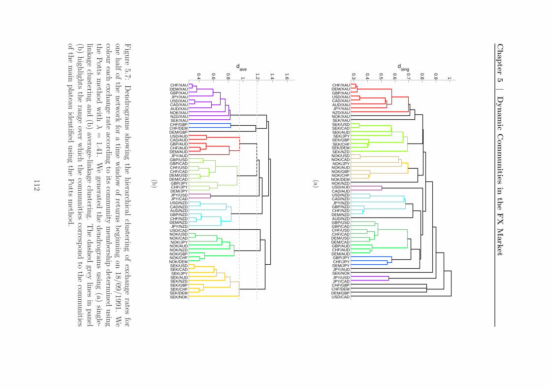
Chapte
r5
|D
ynam
icC
om
munitie
sin
the
FX
Mark
et
0.3
0.4
0.5
0.6
0.7
0.8
0.9 1
CHF/XAUDEM/XAUGBP/XAUUSD/XAUCAD/XAUAUD/XAUJPY/XAUNZD/XAUNOK/XAUSEK/XAUSEK/USDSEK/CADSEK/AUDSEK/JPY
SEK/GBPSEK/CHFSEK/DEMSEK/NZDNOK/USDNOK/CADNOK/JPYNOK/AUDNOK/GBPNOK/CHFNOK/DEMNOK/NZDUSD/AUDCAD/AUDUSD/NZDCAD/NZDJPY/NZDGBP/NZDCHF/NZDDEM/NZDAUD/NZDGBP/USDGBP/CADCHF/USDCHF/CADDEM/USDDEM/CADGBP/AUDCHF/AUDDEM/AUDGBP/JPYCHF/JPYDEM/JPYJPY/AUDSEK/NOKJPY/USDJPY/CADCHF/GBPCHF/DEMDEM/GBPUSD/CAD
dsing
(a)
0.4
0.6
0.8 1
1.2
1.4
1.6
CHF/XAUDEM/XAUGBP/XAUJPY/XAU
USD/XAUCAD/XAUAUD/XAUNOK/XAUNZD/XAUSEK/XAUCHF/GBPCHF/DEMDEM/GBPUSD/AUDCAD/AUDGBP/AUDCHF/AUDDEM/AUDJPY/AUD
GBP/USDGBP/CADCHF/USDCHF/CADDEM/USDDEM/CADGBP/JPYCHF/JPYDEM/JPYJPY/USDJPY/CADUSD/NZDCAD/NZDAUD/NZDGBP/NZDCHF/NZDDEM/NZDJPY/NZD
USD/CADNOK/USDNOK/CADNOK/JPYNOK/AUDNOK/NZDNOK/GBPNOK/CHFNOK/DEMSEK/USDSEK/CADSEK/JPYSEK/AUDSEK/NZDSEK/GBPSEK/CHFSEK/DEMSEK/NOK
dave
(b)
Figu
re5.7:
Den
drogram
ssh
owin
gth
ehierarch
icalclu
stering
ofex
chan
gerates
foron
ehalf
ofth
enetw
orkfor
atim
ew
indow
ofretu
rns
begin
nin
gon
18/09/1991.W
ecolou
reach
exch
ange
rateaccord
ing
toits
comm
unity
mem
bersh
ipdeterm
ined
usin
gth
ePotts
meth
od
with
λ=
1.41.W
egen
eratedth
eden
drogram
susin
g(a)
single-
linkage
clusterin
gan
d(b
)average-lin
kageclu
stering.
The
dash
edgrey
lines
inpan
el(b
)high
lights
the
range
overw
hich
the
comm
unities
correspon
dto
the
comm
unities
ofth
em
ainplateau
iden
tified
usin
gth
ePotts
meth
od.
112

5.7 | Exchange rate centralities and community persistence
5.7 Exchange rate centralities and community per-
sistence
Thus far, we have considered the properties of entire communities. We now investigate
the roles of nodes within communities.
5.7.1 Centrality measures
We describe the relationship between a node and its community using various cen-
trality measures. In the social networks literature, such measures are used to measure
the roles of nodes within the network and to identify which nodes are the most impor-
tant or most prominent [304]. Because there are many notions of importance, several
different centrality measures have been proposed [299]. In the present context, we
use centrality measures to identify exchange rates that occupy important positions
within the FX market.
The betweenness centrality of nodes is defined using the number of geodesic paths
between pairs of vertices in a network [110, 217]. We calculate node betweenness by
taking the distance between nodes i and j as
dij =
0 if i = j or Aij = 1 ,
1/Aij otherwise .(5.12)
The betweenness centrality bi of node i is then given by
bi =∑
s
∑
t
gist
Gst
, for s, t 6= i and s 6= t, (5.13)
where Gst is the total number of shortest paths from node s to node t and gist is the
number of shortest paths from s to t passing through i. Betweenness centrality is
widely used in social network analysis to quantify the extent to which people lie on
paths that connect others. Nodes with high betweenness can be considered to be im-
portant for facilitating communication between others in the network, so betweenness
is used to help measure the importance of nodes for the spread of information around
the network [299].
We also consider the community centrality of each node [220]. We employ the
scaled energy matrix J, with components Jij = Aij − λPij, where we again set Pij =
kikj/2m = (N − 2)/2N . Following the notation in Ref. [220], the energy matrix can
be expressed as J = UDUT , where U = (u1|u2| . . .) is the matrix of eigenvectors of
113
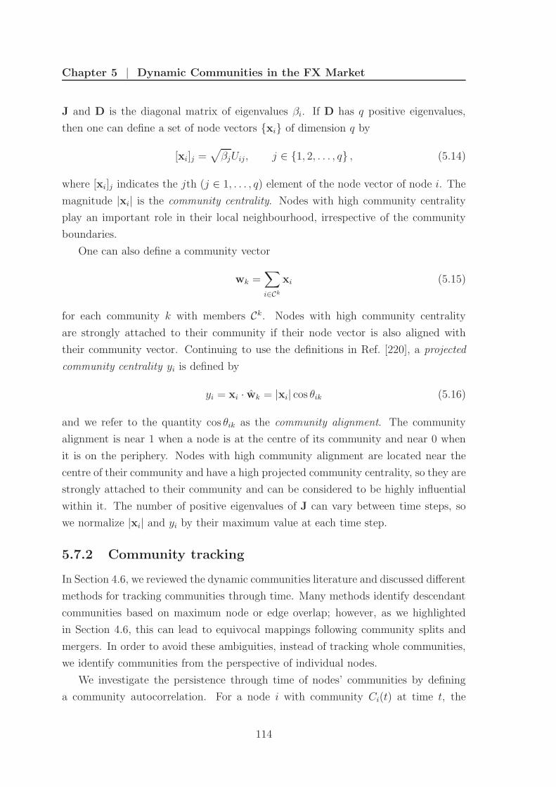
Chapter 5 | Dynamic Communities in the FX Market
J and D is the diagonal matrix of eigenvalues βi. If D has q positive eigenvalues,
then one can define a set of node vectors xi of dimension q by
[xi]j =√
βjUij, j ∈ 1, 2, . . . , q , (5.14)
where [xi]j indicates the jth (j ∈ 1, . . . , q) element of the node vector of node i. The
magnitude |xi| is the community centrality. Nodes with high community centrality
play an important role in their local neighbourhood, irrespective of the community
boundaries.
One can also define a community vector
wk =∑
i∈Ck
xi (5.15)
for each community k with members Ck. Nodes with high community centrality
are strongly attached to their community if their node vector is also aligned with
their community vector. Continuing to use the definitions in Ref. [220], a projected
community centrality yi is defined by
yi = xi · wk = |xi| cos θik (5.16)
and we refer to the quantity cos θik as the community alignment. The community
alignment is near 1 when a node is at the centre of its community and near 0 when
it is on the periphery. Nodes with high community alignment are located near the
centre of their community and have a high projected community centrality, so they are
strongly attached to their community and can be considered to be highly influential
within it. The number of positive eigenvalues of J can vary between time steps, so
we normalize |xi| and yi by their maximum value at each time step.
5.7.2 Community tracking
In Section 4.6, we reviewed the dynamic communities literature and discussed different
methods for tracking communities through time. Many methods identify descendant
communities based on maximum node or edge overlap; however, as we highlighted
in Section 4.6, this can lead to equivocal mappings following community splits and
mergers. In order to avoid these ambiguities, instead of tracking whole communities,
we identify communities from the perspective of individual nodes.
We investigate the persistence through time of nodes’ communities by defining
a community autocorrelation. For a node i with community Ci(t) at time t, the
114

5.7 | Exchange rate centralities and community persistence
autocorrelation ati(τ) of its community after τ time steps is defined by
ati(τ) =
| Ci(t) ∩ Ci(t + τ) || Ci(t) ∪ Ci(t + τ) | . (5.17)
This is a node-centric version of a quantity considered in Ref. [233] and importantly
does not require one to determine which community at each time step represents the
descendant of a community at the previous time step.
5.7.3 Exchange rate roles
In Fig. 5.8(a), we show the mean normalized community centrality of exchange rates
as a function of community size (averaging over all nodes belonging to the same-size
community). The community centrality increases with community size up to sizes
of about 10 members. For larger communities, |xi| remains approximately constant.
Nodes with high |xi| therefore tend to belong to large communities, so exchange rates
with high community centrality tend to be closely linked with many other rates. Ta-
ble 5.2 shows the ten exchange rates that have the highest betweenness centrality,
community centrality, and projected community centrality. For all three periods,
CHF/NZD, CHF/XAU, and SEK/XAU have one of the ten highest community cen-
tralities, so they are closely tied to many other rates. For 1991–2003, exchange rates
formed from one of the major European currencies—DEM (and then EUR, after its
introduction) or CHF—and one of the commodity currencies3 also tend to have high
community centrality. For 2005–2008, however, XAU rates encompass nearly all of
the exchange rates with the highest |xi|.Figure 5.8(b) shows the mean betweenness centrality versus the community align-
ment. We calculate the mean community alignment by splitting the range of b into
10 bins containing equal numbers of data points and then averaging over all commu-
nity alignments falling within these bins. (The observed relationships are robust with
respect to variations in the number of bins.) Nodes with high betweenness centrality
tend to have small values for their community alignment, implying that nodes that are
important for information transfer are usually located on the edges of communities.
Table 5.2 shows that for all three periods, NOK/SEK, AUD/NZD, and AUD/CAD
all tend to have high betweenness centrality on average. They are therefore located on
the edges of communities and are important for information transfer. Interestingly,
for the post-euro period (1999–2008), several USD exchange rates are also impor-
tant for information transfer, but no USD rates regularly have high betweenness for
3A country is said to have a “commodity currency” if its export income depends heavily on acommodity. For example, AUD, NZD and CAD are all considered to be commodity currencies.
115

Chapter 5 | Dynamic Communities in the FX Market
0.4 0.5 0.6 0.7 0.8 0.9 1
0.4
0.5
0.6
0.7
0.8
0.9
1
y
a(τ)
c)
τ=1τ=2τ=5τ=10τ=20τ=50
0 5 10 15 20 25 30 350.75
0.8
0.85
0.9
0.95
1
community size
|x|
a)
0 20 40 60 80 100 120 140
0.82
0.84
0.86
0.88
0.9
0.92
b
cosθ
b)
Figure 5.8: (a) Mean community centrality versus the size of the community to whichthe node belongs. (b) Mean community alignment versus the betweenness central-ity of nodes. (c) Mean community autocorrelation versus the projected communitycentrality. (All error bars indicate the standard error [42].)
the pre-euro period. In contrast, XAU exchange rates are important for information
transfer for the pre-euro period but not after the euro was introduced.
In Fig. 5.8(c), we show the mean community autocorrelation versus the projected
community centrality. We calculate the mean autocorrelation by splitting the range
of y into 15 bins containing equal numbers of data points and then averaging over
all autocorrelations falling within these bins. (Again, the observed relationships are
robust with respect to variations in the number of bins.) As one would expect, the
community autocorrelation for the projected community centrality of a given node is
smaller for larger τ . More interesting is that for all values of τ , the mean community
autocorrelation increases with y. This suggests that nodes that are strongly connected
to their community are likely to persistently share that community membership with
the same subset of nodes. In contrast, exchange rates with a low y experience regular
changes in the set of rates with which they are clustered. This result agrees with the
observation in Ref. [233] for social networks that nodes that are only loosely connected
to their community were more likely to leave that community than nodes with strong
intra-community connections (see Section 4.6.5).
Table 5.2 shows the exchange rates with the highest projected community central-
ity, which in turn reveals the most persistent communities. For 1991–2003, approxi-
116

5.8 | Major community changes
mately half of the ten exchange rates with the highest projected community centrality
also appear in the list of the ten rates with the highest community centrality. For
2005–2008, however, the lists of exchange rates with the highest community centrality
and projected community centrality are dominated by the same set of XAU exchange
rates (though the rankings differ). For 1991–2003, the exchange rates with the high-
est projected community centrality again includes rates formed of DEM (and EUR)
or CHF and one of the commodity currencies. However, there are also a number of
USD exchange rates with high projected community centrality that don’t have high
community centrality. This suggests that these USD rates do not have strong links
with a large number of other exchange rates, but that they strongly influence the
rates within their community.
5.8 Major community changes
We now investigate the insights that short-term community dynamics can provide
into changes in the FX market. Figure 5.9(a) shows a contour plot of the normalized
distribution of the link weights at each time step. The mean link strength remains
constant through time because of the inclusion in the network of each exchange rate
and its inverse but [as one can see in Figs. 5.9(a) and 5.9(b)] there is a large variation
in the standard deviation of the link strengths. The scaled energy and standard
deviation of link weights are closely related. This is expected because the standard
deviation increases as a result of the strengthening of strong ties and the weakening
of weak ties.
In Fig. 5.9(c), we also show V between the community configurations at consec-
utive time steps. Large spikes in V indicate significant changes in the community
configuration over a single time step and potentially also indicate important mar-
ket changes. The correlation coefficient between V and the absolute change in Qs
between consecutive time steps is 0.39 over the period 1991–2003 and 0.47 over the
period 2005–2008. The correlation between V and the absolute change in σ(Aij) is
0.28 over the period 1991–2003 and 0.27 from 2005–2008. Changes in Qs are thus a
better indicator than changes in σ(Aij) that there has been a change in the community
configuration of the network.
In Fig. 5.10, we show three example community reorganizations—two in which V
is more than four standard deviations larger than its mean and a third in which it is
over two standard deviations above the mean.
117
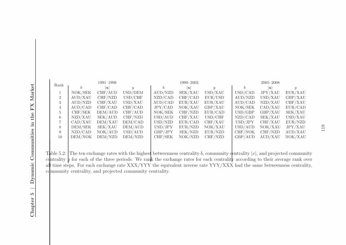
Chapte
r5
|D
ynam
icC
om
munit
ies
inth
eFX
Mark
et Rank
1991–1998 1999–2003 2005–2008b |x| y b |x| y b |x| y
1 NOK/SEK CHF/AUD USD/DEM AUD/NZD SEK/XAU USD/XAU USD/CAD JPY/XAU EUR/XAU2 AUD/XAU CHF/NZD USD/CHF NZD/CAD CHF/CAD EUR/USD AUD/NZD USD/XAU GBP/XAU3 AUD/NZD CHF/XAU USD/XAU AUD/CAD EUR/XAU EUR/XAU AUD/CAD NZD/XAU CHF/XAU4 AUD/CAD CHF/CAD CHF/CAD JPY/CAD NOK/XAU GBP/XAU NOK/SEK CAD/XAU EUR/CAD5 CHF/SEK DEM/AUD CHF/AUD NOK/SEK CHF/NZD EUR/CAD USD/GBP GBP/XAU SEK/XAU6 NZD/XAU SEK/AUD CHF/NZD USD/AUD CHF/XAU USD/CHF NZD/CAD SEK/XAU USD/XAU7 CAD/XAU DEM/XAU DEM/CAD USD/NZD EUR/CAD CHF/XAU USD/JPY CHF/XAU EUR/NZD8 DEM/SEK SEK/XAU DEM/AUD USD/JPY EUR/NZD NOK/XAU USD/AUD NOK/XAU JPY/XAU9 NZD/CAD NOK/AUD USD/AUD GBP/JPY SEK/NZD EUR/NZD CHF/NOK CHF/NZD AUD/XAU10 DEM/NOK DEM/NZD DEM/NZD CHF/SEK NOK/NZD CHF/NZD GBP/AUD AUD/XAU NOK/XAU
Table 5.2: The ten exchange rates with the highest betweenness centrality b, community centrality |x|, and projected communitycentrality y for each of the three periods. We rank the exchange rates for each centrality according to their average rank overall time steps. For each exchange rate XXX/YYY the equivalent inverse rate YYY/XXX had the same betweenness centrality,community centrality, and projected community centrality.
118

5.8 | Major community changes
Aij
0
0.5
1
0
0.05
0.1
Qs
03/10/91 29/06/94 25/03/97 20/12/99 15/09/02 11/06/05 07/03/080
0.2
0.4
date
V
0 0.05 0.1 0.15 0.2 0.25 0.3 0.35 0.4
0.15
0.2
0.25
0.3
σ(A
ij)Qs
σ(Aij)
a)
b)
c)
Figure 5.9: (a) Normalized distribution of the link weights at each time step. (b)Scaled energy Qs (black line) and standard deviation of the link weights (blue line).(c) Normalized variation of information V between the community configurations atconsecutive time steps. The horizontal lines show (from bottom to top) the mean ofV and 1, 2, 3, 4, 5, and 6 standard deviations above the V mean. The green verticalline in panels (b) and (c) separates the pre- and post-euro periods. The red verticallines show the time steps when 22/12/94, 07/02/97, and 15/08/07 enter the rollingtime window. These dates correspond, respectively, to the devaluation of the Thaibaht during the Asian currency crisis, the flotation of the Mexican peso following itssudden devaluation during the tequila crisis, and significant unwinding of the carrytrade during the 2007–2008 credit crisis. The grey blocks mark 2004 (for which wehave no data).
119
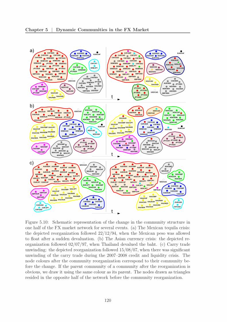
Chapter 5 | Dynamic Communities in the FX Market
Figure 5.10: Schematic representation of the change in the community structure inone half of the FX market network for several events. (a) The Mexican tequila crisis:the depicted reorganization followed 22/12/94, when the Mexican peso was allowedto float after a sudden devaluation. (b) The Asian currency crisis: the depicted re-organization followed 02/07/97, when Thailand devalued the baht. (c) Carry tradeunwinding: the depicted reorganization followed 15/08/07, when there was significantunwinding of the carry trade during the 2007–2008 credit and liquidity crisis. Thenode colours after the community reorganization correspond to their community be-fore the change. If the parent community of a community after the reorganization isobvious, we draw it using the same colour as its parent. The nodes drawn as trianglesresided in the opposite half of the network before the community reorganization.
120

5.8 | Major community changes
5.8.1 Mexican peso crisis
Figure 5.10(a) shows the reorganization on 22/12/1994 when the Mexican peso was
floated following its sudden devaluation.4 This change is accompanied by an increase
in the scaled energy. Although we do not include the Mexican peso in the set of
investigated exchange rates, it appears that its devaluation was a sufficiently serious
event to cause major changes in the community relationships of the studied rates.
Before 22/12/1994, the largest community consisted of a group of exchange rates
constructed from currencies from the set AUD, CAD, NZD, USD, XAU versus
currencies from CHF, DEM, GBP, JPY, NOK. After the flotation, the largest
community consisted of a set of exchange rates formed from the major European
currencies (CHF, DEM, and GBP). It is also noteworthy that there is only a small
gold (XAU) community during this period which, as noted previously, often indicates
that another currency is particularly important in the market.
5.8.2 Asian currency crisis
Figure 5.10(b) shows the community changes following 02/07/1997 when the Thai
baht was devalued during the Asian currency crisis. As with the peso, although we
did not include the baht in the set of studied rates, its devaluation appears to have
had a significant effect on the whole market. There is a large stable gold cluster
during the whole period. Before 02/07/1997, there is also a large AUD cluster, but
after the devaluation, this cluster breaks up and the previously-small GBP cluster
increases in size. This suggests that the GBP is playing a more prominent market
role after the devaluation. Although the reasons for the changes in the sizes of the
AUD and GBP communities are not obvious, both adjustments suggest a sharp and
significant change in the correlation structure of the market.
5.8.3 Credit crisis
The final example in Fig. 5.10(c) shows the community changes following 15/08/07
when there was a significant community reorganization and reveals one of the major
effects on the FX network of the recent credit and liquidity crisis. This example also
demonstrates community changes that occurred as a result of a trading change that
affected the studied rates directly.
4For a floating exchange rate, the value of the currency is allowed to fluctuate according to theFX market. Prior to its floatation the peso had been pegged to the US dollar, so the value of thepeso tracked the value of the dollar.
121

Chapter 5 | Dynamic Communities in the FX Market
The most important effect of the credit crisis on the FX market during the period
2005–2008 was its impact on the carry trade. The carry trade consists of selling
low interest rate funding currencies such as the JPY and CHF and investing in high
interest rate investment currencies such as the AUD and NZD. It yields a profit if the
interest rate differential between the funding and investment currencies is not offset
by a commensurate depreciation of the investment currency [59]. The carry trade is
one of the most commonly used FX trading strategies and requires a strong appetite
for risk, so the trade tends to “unwind” during periods in which there is a decrease in
available credit. A trader unwinds a carry trade position by selling his/her holdings
in investment currencies and buying funding currencies.
One approach to quantifying carry trade activity is to consider the returns that
can be achieved using a carry trade strategy. In Fig. 5.11(b) we show the cumulative
return index Υ for a common carry trade strategy. We consider a strategy in which
one buys equal weights of the three major currencies with the highest interest rates
and sells equal weights of the three currencies with the lowest interest rates. This
is a dynamic trading strategy because the relative interest rates of currencies change
over time. For example, consider the situation in which the interest rate of currency
A (which initially has the third highest interest rate) decreases below the rate of
currency B (which initially has the fourth highest interest rate). In order to maintain
the strategy of only holding the three currencies with the highest interest rates at any
time, one would re-balance the carry portfolio by selling the holding of currency A
and buying currency B. The frequency at which such re-balances occur will depend
on the frequency at which the relative interest rates change. The returns from a carry
strategy like this are widely seen by market participants to provide a good gauge of
carry trade activity. Large negative returns result in large decreases in Υ which are
therefore likely to indicate significant unwinding of the carry trade.
In Fig. 5.11(a) we focus on the period 2005–2008 from Fig. 5.9(c). Again, large
spikes indicate significant changes in the community configuration over a single time
step. Figure 5.11(a) shows that a significant community reorganization occurred on
15/08/07 and in Fig. 5.10(c) we show the observed communities before and after this
date. This community change is a result of massive unwinding of the carry trade.
Figure 5.11(b) shows that leading up to 15/08/07 there was some unwinding of the
carry trade so the initial configuration includes a community containing exchange
rates of the form AUD/YYY, NZD/YYY, and XXX/JPY (which all involve one of
the key carry-trade currencies). In Fig. 5.11(b) it is also clear that following this
date there is a sharp increase in carry unwinding. The second community partition
122
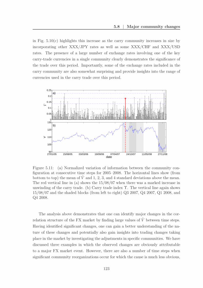
5.8 | Major community changes
in Fig. 5.10(c) highlights this increase as the carry community increases in size by
incorporating other XXX/JPY rates as well as some XXX/CHF and XXX/USD
rates. The presence of a large number of exchange rates involving one of the key
carry-trade currencies in a single community clearly demonstrates the significance of
the trade over this period. Importantly, some of the exchange rates included in the
carry community are also somewhat surprising and provide insights into the range of
currencies used in the carry trade over this period.
0
0.05
0.1
0.15
0.2
0.25
V
a)
date
ϒ
b)
27/01/05 15/08/05 03/03/06 19/09/06 07/04/07 24/10/07 11/05//08 27/11/0890
100
110
120
130
Figure 5.11: (a) Normalized variation of information between the community con-figuration at consecutive time steps for 2005–2008. The horizontal lines show (frombottom to top) the mean of V and 1, 2, 3, and 4 standard deviations above the mean.The red vertical line in (a) shows the 15/08/07 when there was a marked increase inunwinding of the carry trade. (b) Carry trade index Υ. The vertical line again shows15/08/07 and the shaded blocks (from left to right) Q3 2007, Q4 2007, Q1 2008, andQ4 2008.
The analysis above demonstrates that one can identify major changes in the cor-
relation structure of the FX market by finding large values of V between time steps.
Having identified significant changes, one can gain a better understanding of the na-
ture of these changes and potentially also gain insights into trading changes taking
place in the market by investigating the adjustments in specific communities. We have
discussed three examples in which the observed changes are obviously attributable
to a major FX market event. However, there are also a number of time steps when
significant community reorganizations occur for which the cause is much less obvious,
123

Chapter 5 | Dynamic Communities in the FX Market
and the analysis of dynamic communities might help shed light on related market
changes.
5.9 Visualizing changes in exchange rate roles
We now investigate changes in the relationships between specific exchange rates and
their communities. We begin by defining within-community z-scores, which directly
compare the relative importances of different nodes to their community [139]. We
describe the roles of individual nodes at each time step using the within-community
projected community centrality z-score κy and within-community betweenness cen-
trality z-score κb. If a node i belongs to community Ci and has projected community
centrality yi, then
κyi =
yi − yCi
σyCi
, (5.18)
where yCiis the mean of y over all nodes in Ci and σy
Ciis the standard deviation of y
in Ci. The quantity κyi measures how strongly connected node i is to its community
compared with other nodes in the same community. Similarly, if the same node has
betweenness centrality bi, then
κbi =
bi − bCi
σbCi
, (5.19)
where bCiis the average of b over all nodes in Ci and σb
Ciis the standard deviation
of b in Ci. The quantity κbi indicates the importance of node i to the spread of
information compared with other nodes in its community.5 The positions of nodes
in the (κb, κy) plane thereby illuminate the roles of the associated exchange rates in
the FX market and provide information that cannot be gained by simply considering
individual exchange rate time series.
We remark that the methods are robust with respect to the choice of measures used
to construct the parameter plane: we obtain similar results using other notions, such
as dynamical importance [256] instead of the betweenness centrality and the within-
community strength z-score [139] instead of the projected community centrality.
5.9.1 Average roles
In Fig. 5.12, we show the mean position of each exchange rate over the three periods
and highlight some rates that play particularly prominent roles. For example, the
5Note that in order for a within-community z-score to be well defined, a node must belong to acommunity containing two or more nodes.
124

5.9 | Visualizing changes in exchange rate roles
USD/DEM (and then EUR/USD after the introduction of the euro) regularly had
the strongest connection to its community from 1991-2003, but EUR/XAU was more
strongly connected to its community from 2005–2008. The importance of USD/DEM
and EUR/USD is unsurprising given that these rates had the highest daily trading
volume [117]. This provides a reality check that the methods uncover useful in-
formation about the roles of minor exchange rates. Other exchange rates, such as
NOK/SEK and AUD/NZD, were less influential within their communities but were
very important for the transfer of information around the network.
The (κb, κy) plots also highlight exchange rates that play similar roles in the
FX market. For example, exchange rates formed from one of the major European
currencies—DEM or CHF—and one of the commodity currencies—AUD, CAD, and
NZD (or the commodity XAU)—are located close together in the upper left quadrant
of the (κb, κy) plane for 1991–2003. This prominent similarity is not present for
2005–2008.
5.9.2 Annual roles
We can also gain insights into the time dynamics of exchange rate roles by examining
changes in the positions of the rates in the (κb, κy) plane over different time periods.
Changes in a node’s position in the (κb, κy) plane reflect changes in the membership of
a node’s community as well as changes in b and y. In Fig. 5.13, we show six example
annual role evolutions. We determine the annual roles by averaging κy and κb over
all time steps in each year. We see, for example, that the NZD/JPY exchange rate
maintained a consistently influential role within its community over the full period
and similarly the EUR/USD rate also maintained the same influential role played by
the USD/DEM rate before the introduction of the euro.
Other rates changed role over the studied period. The GBP/USD and GBP/CHF
exchange rates evolved in a similar manner, as they changed from being strongly
influential within their communities before 1994 to being less influential within their
communities but more important for information transfer after 1994. The role of both
GBP/AUD and USD/JPY varied significantly from 1991–2008: From 2001 onwards
the GBP/AUD became less influential within its community but more important for
information transfer. Interestingly, the USD/JPY had its highest within-community
influence in the late 1990s during a period of Japanese economic turmoil. One can
construct similar plots to study the change in the role of other exchange rates. These
role plots provide a useful tool for visualizing the changes in the exchange rate corre-
lations.
125

Chapter 5 | Dynamic Communities in the FX Market
κb
κy
−1 −0.5 0 0.5 1 1.5 2
−1.5
−1
−0.5
0
0.5
1
1.5
−2
USD/DEM
USD/CHF
CHF,DEM/commodity
DEM/CHF
NOK/SEK
AUD/XAU
AUD/NZD
USD/XAU
USD/AUD
other
a)
κb
κy
−1 1.5 2−0.5 0 0.5 1
−1.5
−1
−0.5
0
0.5
1
1.5
−2
EUR/USD
USD/CHF
USD/XAU
CHF,EUR/commodity
EUR/CHF
AUD/NZD
AUD/CAD
other
b)
κb
κy
−1 −0.5 0 0.5 1 1.5 2
−1.5
−1
−0.5
0
0.5
1
1.5
−2
EUR/USD
EUR/XAU
EUR/CAD
EUR/CHF
AUD/NZD
USD/CAD
CHF/XAU
NZD/XAU
other
c)
Figure 5.12: Node positions in the (κb, κy) plane averaged over all time steps for theperiods (a) 1991–1998, (b) 1999–2003, and (c) 2005–2008. The radii of each ellipticalmarker equal the standard deviations in the parameters for the corresponding nodescaled by a factor of 1/15 for visual clarity.
126

5.9 | Visualizing changes in exchange rate roles
USD/DEM(EUR/USD)
κy
−2
−1
0
1
2
GBP/CHF
−1 0 1 2
−2
−1
0
1
2
USD/GBP
GBP/AUD
κb−1 0 1 2
USD/JPY
NZD/JPY
−1 0 1 2
19911992199319941995199619971998199920002001200220032005200620072008
Figure 5.13: Annual node role evolutions in the (κb, κy) plane for the full period1991–2008.
5.9.3 Quarterly roles
We also investigate higher-frequency changes in exchange rate market role over shorter
time intervals. In Fig. 5.14 we show quarterly roles changes over the period 1995–1998
for six exchange rates including USD/DEM and GBP/USD for which we also show
the annual changes in Fig. 5.13. Both exchange rates show similar role variations
over both time-scales, with the USD/DEM always playing a relatively influential role
within its community and the GBP/USD role varying significantly. We also show
other examples for which we did not show annual changes. The role of DEM/JPY
varied considerably from 1995–1998: In particular, it was an important information
carrier for the last two quarters in 1996, but was influential within its community
throughout 1998. In contrast the AUD/JPY moves from being unimportant for in-
formation transfer to being an information carrier during 1998. In further contrast,
the AUD/NZD and AUD/XAU were both always information carriers to different ex-
tents, with AUD/NZD being particularly important for information transfer during
1998.
Finally, we consider some examples of quarterly role evolutions for the period
2005–2008. Figure 5.15, shows quarterly role changes for four exchange rates from
2005–2008. The USD/XAU rate provides an interesting example due to the per-
sistence of its community over this period. From 2005–2008, the USD/XAU node
shifted from being an important information carrier within the XAU community to
127

Chapter 5 | Dynamic Communities in the FX Market
being more central to this community. This period of higher influence coincides closely
with the period of financial turmoil during 2007–2008. The CHF is widely regarded as
a “safe haven” currency [248], so one might expect USD/CHF to behave in a similar
manner to USD/XAU. However, the CHF is also a key carry trade currency. Because
CHF is used both as a safe haven and as a carry trade currency, the USD/CHF node
does not move in the same direction as USD/XAU in the (κb, κy) plane. Instead, the
USD/CHF exchange rate is an important information carrier during the 2007–2008
credit crisis. Over the same period, the AUD/JPY and NZD/JPY exchange rates
change from being important for information transfer to being influential within their
communities. The AUD/JPY and NZD/JPY were most influential within their com-
munity during Q3 and Q4 2007 and during Q1 and Q4 2008. Figure 5.11(b) shows
that over all of these periods there was significant carry trade activity so it is unsur-
prising that two exchange rates that are widely used for this trade should increase in
importance. This, however, is a further demonstration that the positions of exchange
rates in the (κb, κy) parameter plane can provide important insights into the role of
exchange rates in the FX market.
USD/DEM
κy
−2
−1
0
1
2
AUD/JPY
−1 0 1 2
−2
−1
0
1
2
GBP/USD
AUD/NZD
κb−1 0 1 2
DEM/JPY
AUD/XAU
−1 0 1 2
Q1 95Q2 95Q3 95Q4 95Q1 96Q2 96Q3 96Q4 96Q1 97Q2 97Q3 97Q4 97Q1 98Q2 98Q3 98Q4 98
Figure 5.14: Quarterly node role evolutions in the (κb, κy) plane for the period 1995–1998.
128

5.10 | Robustness of results
Q1 05Q2 05Q3 05Q4 05Q1 06Q2 06Q3 06Q4 06Q1 07Q2 07Q3 07Q4 07Q1 08Q2 08Q3 08Q4 08
NZD/JPY
κb
−1 0 1 2 3
AUD/JPY
−1 0 1 2 3
−2
−1
0
1
2
USD/XAUUSD/CHF
κy
−2
−1
0
1
2
Figure 5.15: Quarterly node role evolutions in the (κb, κy) plane for the period 2005–2008.
5.10 Robustness of results: alternative computa-
tional heuristics
Thus far, we have detected all communities using a greedy algorithm [44]. However,
as we noted in Chapter 4, several alternative heuristics exist. In Ref. [128], Good et al.
demonstrated that there is extreme degeneracy in the energy function (Eq. 4.3), with
an exponential number of high-energy solutions. Given this, it is unsurprising that,
in some instances, different energy-optimization heuristics have been found to yield
very different partitions for the same network. Good et al. suggest that the reason
for this behaviour is that different heuristics sample different regions of the energy
landscape. Because of the potential sensitivity of results to the choice of heuristic,
one should treat individual partitions output by particular heuristics with caution.
However, one can have more confidence in the validity of the partitions if different
heuristics produce similar results.
With this in mind, we compared the results for the greedy algorithm [44] with those
for a spectral algorithm [221] and simulated annealing [141] for the 563 networks we
constructed for the period 2005–2008. We found that, although there are differences
in the communities identified using different optimization heuristics, the aggregate
129

Chapter 5 | Dynamic Communities in the FX Market
conclusions are the same. We identify the same changes taking place in the FX market
whether we use the greedy algorithm or simulated annealing to minimize energy. The
fact that we obtain very similar results using different optimization techniques, despite
these techniques sampling different regions of the energy landscape, gives confidence
that the effects that we uncover are genuine and that the results are robust. We
present the results of the comparison of the computational heuristics in detail in
Appendix B.
5.11 Summary
We have demonstrated that a network analysis of the FX market is useful for visualiz-
ing and providing insights into the correlation structure of the market. In particular,
we investigated community structure at different times to provide insights into the
clustering dynamics of exchange rate time series. We focused on a node-centric com-
munity analysis that allows one to follow the time dynamics of the functional role of
exchange rates within the market, demonstrating that there is a relationship between
an exchange rate’s functional role and its position within its community. We indi-
cated that exchange rates that are located on the edges of communities are important
for information transfer in the FX market, whereas exchange rates that are located
in the centre of their community have a strong influence on other rates within that
community. We also demonstrated that the community structure of the market can
be used to determine which exchange rates dominate the market at each time step
and identified exchange rates that experienced significant changes in market role.
Our analysis successfully uncovered significant structural changes that occurred in
the FX market, including ones that resulted from major market events that did not
impact the studied exchange rates directly. We further demonstrated that community
reorganizations at specific time steps can provide insights into changes in trading
behaviour and highlighted the prevalence of the carry trade during the 2007–2008
credit and liquidity crisis. Although we focused on networks of exchange rates, the
methodology should be similarly insightful for multivariate time series of other asset
classes. Importantly, the results are robust with respect to the choice of optimization
heuristic.
130

Chapter 6
A Taxonomy of Networks
We now expand the scope of our analysis beyond financial markets and investigate
the community structure of networks from a wide variety of other fields. We have
submitted a paper based on this work for publication [P4].
6.1 Introduction
The study of networks is an interdisciplinary endeavour, with contributions from
researchers in the natural, social, and information sciences [9, 60, 217, 223]. Often
the questions asked by researchers in these different fields are quite similar; however,
techniques have sometimes had difficulty penetrating disciplinary boundaries, perhaps
because the relevance or applicability of the methods from other disciplines is not
always clear. In this chapter, we attempt to connect disciplines by introducing a
framework for clustering networks and using this technique to establish a network
taxonomy. The clustering scheme and taxonomy serve several purposes. First, if
networks from two different fields are close together in the taxonomy, this implies that
there are some similarities in their structure and that techniques from one field might
be insightful in the other field. Second, a taxonomy might help to determine how an
unstudied network might best be analyzed once its position within the taxonomy is
known. Third, the taxonomy can be used to highlight differences within disciplines.
For example, if a network that is expected to be similar to a group of networks based
on their origin is not clustered with those networks, this suggests that the network is
not typical of its family.
In aiming to cluster networks, it is necessary to consider a scale at which to
investigate their structure. Much prior research on networks has focused on micro-
scopic properties (such as the degree) or macroscopic properties (such as the average
131

Chapter 6 | A Taxonomy of Networks
path length), typically finding that most empirically observed networks have heavy-
tailed degree distributions and possess the small-world property (see Section 1.1 and
Refs. [9, 60, 217, 223]). The interpretations of both approaches often implicitly as-
sume that networks are homogeneous and have no mesoscopic structure; however,
as discussed in detail in Chapter 4 and demonstrated in Chapter 5, many networks
possess community structures. The ubiquity of heavy-tailed degree distribution and
the small-world property across a wide variety of networks from different domains
suggests that mesoscopic heterogeneities should be exploited to differentiate effec-
tively between networks. This has led some researchers to try to cluster networks
based on mesoscopic structures, e.g., [142, 210]. In Ref. [142], Milo et al. compare
the statistics of a priori specified subgraphs in networks from different fields, while
in Ref. [142] Guimera et al. investigate the relationships between individual nodes
and communities (see Section 4.5 for a detailed discussion of these methods). Both
approaches focus on a single mesoscopic scale.
In this chapter, we introduce a framework for clustering networks by identifying
communities at multiple mesoscopic scales and create a taxonomy of networks using
this approach. In addition to the fact that mesoscopic heterogeneities enable us to
differentiate between networks, we focus on mesoscopic scales because structures at
this scale have been shown to have a strong bearing on functional units in many
networks [105,244]. In contrast to Ref. [210], we do not specify the topology or sizes
of the structure that we investigate a priori. Networks from different domains can
possess very different sizes and connectivities, which makes comparison difficult [210].
The technique that we propose therefore involves a normalization that enables us
to compare networks of significantly different sizes and connectivities.1 Using this
approach, we create a taxonomy of 714 networks from a variety of disciplines including
sociology, biology, politics, technology, and finance, and include many synthetic model
and benchmark networks. As well as creating an aggregate taxonomy, we also create
taxonomies for sub-sets of networks that represent multiple realizations of the same
type of system and temporal snapshots of time-dependent systems. In the latter case,
we demonstrate that the framework we propose can detect changes in time-ordered
sequences of evolving networks.
1We study networks that range in size from 34 to over 40,000 nodes and possess from 0.1% to100% of possible edges.
132

6.2 | Multi-resolution community detection
6.2 Multi-resolution community detection
In order to compare networks, we create profiles that characterize each network’s
structures across multiple mesoscopic scales. The first step in constructing these
profiles is to select a community detection method. As in the earlier chapters in this
thesis, we detect communities using the the multi-resolution Potts method described
in Section 4.3.3. The Hamiltonian of the infinite-range N -state Potts spin glass is
given by
H(λ) = −∑
i6=j
Jijδ(Ci, Cj) = −∑
i6=j
(Aij − λPij) δ(Ci, Cj), (6.1)
where Ci indicates the state (community) of spin i, λ is a resolution parameter, and
we again use the standard random null model Pij = kikj/(2m), where ki denotes the
degree of node i for an unweighted network (the strength for a weighted network)
and m is the number of edges for an unweighted network (or the total edge weight
for weighted networks) [224].2 By tuning the resolution parameter λ, we detect com-
munities across multiple scales.
6.2.1 Resolution matrix
The second step is to determine the range of values of λ to investigate. We study a
wide variety of networks containing different numbers of nodes and edges; to ensure
that the profiles for different networks are comparable, we sweep λ from the minimum
value Λmin to the maximum value Λmax, so that the number of communities η into
which the network is partitioned varies from 1 to the number of nodes N in the
network.
More formally, we define a coupling matrix J(λ) with entries Jij(λ) that represent
the interaction strength between node i and j in the Potts Hamiltonian in Eq. 6.1.
For each pair of nodes i and j, we find the resolution λ = Λij at which the interaction
Jij between them becomes antiferromagnetic by writing Jij = Aij − ΛijPij = 0 and
solving to get Λij = Aij/Pij. We then define a matrix Λ with entries Λij and define
three resolutions:
Λmin = maxij
Λij |η(λ) = 1 , (6.2)
Λmax = maxij
Λij + ǫ, (6.3)
Λ∗ = minij
Λij |Aij > 0 , (6.4)
2In Chapter 5, we summed over all i and j in the Potts Hamiltonian (see Eq. 4.3). In contrast,in this chapter, we only sum over all i 6= j. We explain the reason for this difference in Section D.1.
133

Chapter 6 | A Taxonomy of Networks
where ǫ > 0 is a small number that ensures that all links are antiferromagnetic at
resolution λ = Λmax. In other words, Λmin is the largest value of the resolution
parameter λ for which the network still forms a single community. However, note
that this is not necessarily the minimum non-zero value of Λij. We do not simply
sweep over the interval [Λ∗, Λmax] because for some sparse networks η > 1 at Λ∗,
whereas for fully-connected networks η does not become greater than one until a
resolution λ ≫ Λ∗. By sweeping λ from Λmin to Λmax, and exploring the full range
of partitions from η = 1 to η = N , we ensure that the profiles are comparable for
different networks.
6.2.2 Problems with comparing networks using resolution
The most common method for studying network community structure across multiple
mesoscopic scales is to consider plots of networks summary statistics as a function
of the resolution parameter, e.g., [17, 105, 244, 254].3 However, there are problems
with this approach for some networks. Consider, Fig. 6.1(a), which shows the cu-
mulative distribution P (Λij ≤ x) for an (unweighted) network of Facebook users at
Caltech [295].4 The vast majority of Λij values are less than 100, but there are a few
interactions with Λij > 8000. The large Λij values are the result of two low degree
nodes being connected. Using the standard null model Pij = kikj/(2m), the inter-
action between two nodes i and j becomes antiferromagnetic when λ > Aij/Pij =
2mAij/(kikj). If there are a large number of edges in the network, but both i and j
have very low degrees, λ needs to be large to make the interaction antiferromagnetic.
Figure 6.1(b) demonstrates the effect of these interactions on a plot of the number of
communities η as a function of λ over the interval [Λmin, Λmax] for the Caltech net-
work. The network breaks up into just under N communities over a small range of λ,
but there is then a long plateau as a few interactions with large λ become antiferro-
magnetic and the remaining communities break up. These few interactions dominate
the figure and obscure the structure at small resolutions.
One way of avoiding this problem is only to sweep λ over a range such that the
number of communities varies between η ∈ [1, fN ], where fN is some fraction of the
total number of nodes in the network. Using this approach, it would not be necessary
to force the nodes with large Λij into individual communities, so the range of λ would
be significantly smaller. However, there are obvious problems with this method: first,
the choice of f is arbitrary; second, in general, the value of f that avoids the long
3In Chapter 5 we use this approach to study communities in FX market networks.4We enumerate all of the networks that we study in Table C.1 in Appendix C.
134

6.2 | Multi-resolution community detection
plateaus is different for different networks; if one wishes to use plots of summary
statistics versus resolution to compare networks, the value of f ought to be constant.
Therefore, this seems like an unsuitable solution.
0 1000 2000 3000 4000 5000 6000 7000 80000
100
200
300
400
500
600
700
800
λ
η
1 100 1000 80000
0.2
0.4
0.6
0.8
1
Λij
P(Λ
ij≤x)
Figure 6.1: A demonstration using the Caltech Facebook network [295] of the prob-lem of using the resolution parameter for networks with low-degree nodes that areconnected to each other. The left figure shows the cumulative distribution of Λij
values P (Λij ≤ x); the majority of Λij are less than 100, but there are a few nodeswith Λij > 8000. The right figure shows the number of communities as a functionof λ and demonstrates that the presence of low strength nodes that are connected toeach other results in a long plateau. Only a few interactions then dominate the plotand obscure the structure at smaller λ.
Of course, the problem of having interactions that require large λ to become
antiferromagnetic stems initially from our choice of null model. An alternative choice
of null model that avoids this problem is one in which Pij is constant for all i and
j. In contrast to the standard null model Pij = kikj/(2m), however, this model does
not preserve the strength distribution of the original network. Given this appealing
property of the null model Pij = kikj/(2m) and its ubiquity within the literature, we
persevere with this model.
6.2.3 Effective fraction of antiferromagnetic links
To avoid the issues arising from a few interactions requiring large resolutions to be-
come antiferromagnetic, instead of considering network properties as a function of the
resolution parameter, we work in terms of the effective fraction of antiferromagnetic
links ξ. We define ξ as
ξ = ξ(λ) =ℓA(λ) − ℓA(Λmin)
ℓA(Λmax) − ℓA(Λmin), (6.5)
135
Chapter 6 | A Taxonomy of Networks
where ℓA(λ) is the total number of antiferromagnetic interactions (Jij < 0) in the
system for the given value of λ and ℓA(Λmin) is the largest number of antiferromag-
netic interactions for which the network still forms a single community. The effective
number of antiferromagnetic interactions ξ(λ) is therefore the number of antiferro-
magnetic interactions in excess of ℓA(Λmin) (normalized to the unit interval) and is a
monotonically increasing function of λ.
To simplify the discussion of the fraction of antiferromagnetic links, it is also
useful to divide the elements of the adjacency matrix A into links (Aij > 0) and non-
links (Aij = 0). Based on the values Λij, we further distinguish between two types
of links: links with 0 < Λij ≤ Λmin are called Λ−-links, and links with Λij > Λmin
are called Λ+-links. The sum of the number of Λ−-links and Λ+-links is then equal
to L, the number of links in the network.5 When λ = Λmin all of the Λ−-links are
antiferromagnetic, but the network nevertheless consists of a single community.
We illustrate the differences between the different types of links in Fig. 6.2 in which
we show examples of the cumulative distributions of links P (Λij ≤ x) for a fully-
connected, weighted network and for an unweighted network. For the unweighted
network, Λmin < Λ∗, so the network does not possess any Λ−-links. As one increases
the resolution parameter, the network begins to break up into communities before
any of the Λ+-links become antiferromagnetic. In contrast, for the fully-connected,
weighted network Λ∗ < Λmin.
6.2.3.1 Properties of the fraction of antiferromagnetic links
In the definition of ξ that we select, we sweep over the values λ ∈ [Λmin, Λmax], so that
the number of communities varies between 1 and N . Although the regime λ < Λmin
affects the energy H(λ) (see Eq. 6.1), there are no further changes in the partition into
communities and, consequently, only the region λ ∈ [Λmin, Λmax] is interesting. The
normalization in our definition of ξ accounts for the existence of antiferromagnetic
Λ−-links, which do not cause the network to break up into communities and ensures
that 0 ≤ ξ ≤ 1. Note that ξ is equal to the fraction of antiferromagnetic Λ+-links.
By working in terms of ξ rather than λ, we ensure that interactions that require
a large resolution to become antiferromagnetic do not dominate plots of community
summary statistics. The existence of such interactions also implies that we do not
necessarily sweep λ uniformly over the interval [Λmin, Λmax]. As demonstrated in
Fig. 6.1, some networks have several orders of magnitude between Λmin and Λmax and
most interactions become antiferromagnetic at λ ≈ Λmin. To ensure that ξ is sampled
5In an unweighted network L = m, the total link weight in the network.
136

6.3 | Mesoscopic response functions
0 1 2 30
0.1
0.2
0.3
0.4
0.5
0.6
0.7
0.8
0.9
1P
(Λij≤x
)
Λij
Λ− links Λ+ links Λ* Λmin
Λmax
0 20 40 60 80 1000
0.1
0.2
0.3
0.4
0.5
0.6
0.7
0.8
0.9
1
P(Λ
ij≤x)
Λij
Λ+ links Λ* Λmin
Λmax
Figure 6.2: The cumulative distribution P (Λij ≤ x) for: (left) the 100th U.S. Houseof Representatives roll-call voting network [203,241,306], (right) the dolphins network[192]. We show the proportions of Λ+ and Λ− links in the distributions and highlightthe position of Λ∗, Λmin, and Λmax. For the House network, Λmin > Λ∗, so there areboth Λ+ and Λ− links. For the dolphins network, Λmin < Λ∗, so all links are Λ+ linksand the network begins to break up into communities at a resolution λ ≤ Λmin.
uniformally, we select the values of λ using the cumulative distribution of Λij for
Λ+-links, instead of simply sampling λ uniformally over the interval [Λmin, Λmax].6
In Appendix D we provide further technical details of the Potts Hamiltonian and
of the structure of the networks that we study.
6.3 Mesoscopic response functions
The third step in creating multi-resolution profiles to characterize a network’s meso-
scopic structures is to select summary statistics to examine as a function of ξ. We
choose to investigate the number of communities η, the energy H (given by Eq. 6.1)
and the partition entropy S (given by Eq. 5.6).7 The values of these quantities vary
across networks; for example, as we show in Section D.1, the energy H is determined
6As we noted in Section 4.3.3, the number of possible community partitions grows rapidly with thenumber of nodes [218], so finding communities in large networks is computationally intensive [55]. Asa result, one cannot find the optimal community configuration at every resolution and, accordingly,the values of Λmin that we find are necessarily approximate.
7We focus on the energy, entropy and number of communities because, as we discuss later inthis section, each statistic provides information on a key property of the community structure of thenetworks. One could examine other summary statistics as a function of ξ; however, in the interestsof parsimony, it is desirable to limit the number of summary statistics. In Section 6.4.1 we use PCAto construct a single measure that summarize the three statistics.
137

Chapter 6 | A Taxonomy of Networks
by the resolution λ, and Λmax depends strongly on the link structure of the network.
As a result, for it to be possible to compare networks using profiles of the summary
statistics versus ξ, we need to normalize H, S, and η. Therefore, we define an effective
energy as
Heff(λ) =H(λ) −Hmin
Hmax −Hmin= 1 − H(λ)
Hmin, (6.6)
where Hmin = H(Λmin) and Hmax = H(Λmax). Similarly, we define an effective entropy
Seff(λ) =S(λ) − Smin
Smax − Smin=
S(λ)
log N, (6.7)
where Smin = S(λmin) and Smax = S(λmax), and an effective number of communities
ηeff(λ) =η(λ) − ηmin
ηmax − ηmin
=η(λ) − 1
N − 1, (6.8)
where ηmin = η(Λmin) and ηmax = η(Λmax). In sweeping ξ from 0 to 1, the number
of communities increases from η(ξ = 0) = 1 to η(ξ = 1) = N , producing a signature
that we call the mesoscopic response function (MRF). Because Heff ∈ [0, 1], Seff ∈[0, 1], ηeff ∈ [0, 1], and ξ ∈ [0, 1] for any network, we can compare the response
functions across networks and use the MRFs to identify groups of networks with
similar mesoscopic structures.
For a given network, at each resolution, Heff, Seff, and ηeff respectively provide
a measure of the frustration level of the spin system, the disorder in the associated
community size distribution (whether most nodes are in a few large communities or
are spread across many small communities), and the number of communities. The
MRFs indicate the way in which these quantities change as the resolution parameter
is increased – at higher resolutions there is a larger incentive for nodes to belong to
smaller communities, so communities fragment. The shapes of the MRFs (gradient,
concavity/convexity, points of inflection etc.) are the non-trivial result of many fac-
tors, including the fraction of possible edges in the network; the relative weights of
inter- versus intra-community edges; the edge weights compared with the expected
edge weights in the random null model; the number of edges that need to become
antiferromagnetic for a community to fragment; and the way in which the commu-
nities fragment (e.g., whether a single node leaves a community if an edge becomes
antiferromagnetic or a community splits in half). The effects of some of these factors
on the shapes of the MRFs can be better understood by considering some examples.
138
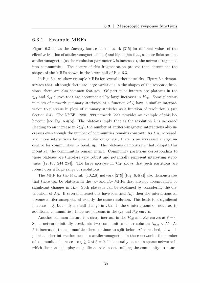
6.3 | Mesoscopic response functions
6.3.1 Example MRFs
Figure 6.3 shows the Zachary karate club network [315] for different values of the
effective fraction of antiferromagnetic links ξ and highlights that, as more links become
antiferromagnetic (as the resolution parameter λ is increased), the network fragments
into communities. The nature of this fragmentation process then determines the
shapes of the MRFs shown in the lower half of Fig. 6.3.
In Fig. 6.4, we show example MRFs for several other networks. Figure 6.4 demon-
strates that, although there are large variations in the shapes of the response func-
tions, there are also common features. Of particular interest are plateaus in the
ηeff and Seff curves that are accompanied by large increases in Heff. Some plateaus
in plots of network summary statistics as a function of ξ have a similar interpre-
tation to plateaus in plots of summary statistics as a function of resolution λ (see
Section 5.4). The NYSE: 1980–1999 network [229] provides an example of this be-
haviour [see Fig. 6.4(b)]. The plateaus imply that as the resolution λ is increased
(leading to an increase in Heff), the number of antiferromagnetic interactions also in-
creases even though the number of communities remains constant. As λ is increased,
and more interactions become antiferromagnetic, there is an increased energy in-
centive for communities to break up. The plateaus demonstrate that, despite this
incentive, the communities remain intact. Community partitions corresponding to
these plateaus are therefore very robust and potentially represent interesting struc-
tures [17, 105, 244, 254]. The large increase in Heff shows that such partitions are
robust over a large range of resolutions.
The MRF for the Fractal: (10,2,8) network [279] [Fig. 6.4(k)] also demonstrates
that there can be plateaus in the ηeff and Seff MRFs that are not accompanied by
significant changes in Heff. Such plateaus can be explained by considering the dis-
tribution of Λij. If several interactions have identical Λij, then the interactions all
become antiferromagnetic at exactly the same resolution. This leads to a significant
increase in ξ, but only a small change in Heff. If these interactions do not lead to
additional communities, there are plateaus in the ηeff and Seff curves.
Another common feature is a sharp increase in the Heff and Seff curves at ξ = 0.
Some networks initially break into two communities at a resolution Λmin < Λ∗. As
λ is increased, the communities then continue to split before Λ∗ is reached, at which
point another interaction becomes antiferromagnetic. In these networks, the number
of communities increases to η ≥ 2 at ξ = 0. This usually occurs in sparse networks in
which the non-links play a significant role in determining the community structure.
139

Chapter 6 | A Taxonomy of Networks
ξ = 0, η = 1 ξ = 0.2, η = 8 ξ = 0.4, η = 12
ξ = 0.6, η = 17 ξ = 0.8, η = 24 ξ = 1, η = 34
ξ = 0.2
ξ = 0.4 ξ = 0.6 ξ = 0.8ξ = 0 ξ = 1
0
0.2
0.4
0.6
0.8
1
ξ
Heff
Seff
ηeff
non−links antiferromagnetic linksferromagnetic links
Figure 6.3: The upper half of the figure shows the Zachary karate club network[315] for different values of the effective fraction of antiferromagnetic links ξ. Theedges are coloured blue if the corresponding interaction is ferromagnetic or red if theinteraction is antiferromagnetic. The nodes are coloured according to their communitymembership. In the lower half of the figure, we show the Heff, Seff, and ηeff MRFsand the interaction matrix J for different values of ξ. We have coloured elements ofthe interaction matrix corresponding to non-links white and elements correspondingto ferromagnetic and antiferromagnetic links blue and red, respectively.
140
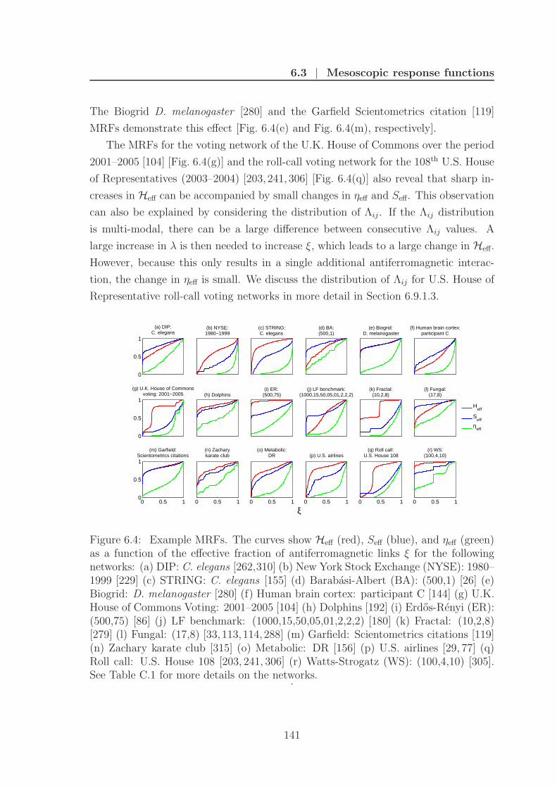
6.3 | Mesoscopic response functions
The Biogrid D. melanogaster [280] and the Garfield Scientometrics citation [119]
MRFs demonstrate this effect [Fig. 6.4(e) and Fig. 6.4(m), respectively].
The MRFs for the voting network of the U.K. House of Commons over the period
2001–2005 [104] [Fig. 6.4(g)] and the roll-call voting network for the 108th U.S. House
of Representatives (2003–2004) [203, 241, 306] [Fig. 6.4(q)] also reveal that sharp in-
creases in Heff can be accompanied by small changes in ηeff and Seff. This observation
can also be explained by considering the distribution of Λij . If the Λij distribution
is multi-modal, there can be a large difference between consecutive Λij values. A
large increase in λ is then needed to increase ξ, which leads to a large change in Heff.
However, because this only results in a single additional antiferromagnetic interac-
tion, the change in ηeff is small. We discuss the distribution of Λij for U.S. House of
Representative roll-call voting networks in more detail in Section 6.9.1.3.
0
0.5
1
(a) DIP:C. elegans
(b) NYSE:1980−1999
(c) STRING:C. elegans
(d) BA:(500,1)
(e) Biogrid:D. melanogaster
(f) Human brain cortex:participant C
0
0.5
1
(g) U.K. House of Commonsvoting: 2001−2005
(h) Dolphins
(i) ER: (500,75)
(j) LF benchmark:(1000,15,50,05,01,2,2,2)
(k) Fractal:(10,2,8)
(l) Fungal:(17,8)
0 0.5 10
0.5
1
(m) Garfield:Scientometrics citations
0 0.5 1
(n) Zacharykarate club
0 0.5 1
(o) Metabolic:DR
ξ0 0.5 1
(p) U.S. airlines
0 0.5 1
(q) Roll call:U.S. House 108
0 0.5 1
(r) WS:(100,4,10)
Heff
Seff
ηeff
Figure 6.4: Example MRFs. The curves show Heff (red), Seff (blue), and ηeff (green)as a function of the effective fraction of antiferromagnetic links ξ for the followingnetworks: (a) DIP: C. elegans [262,310] (b) New York Stock Exchange (NYSE): 1980–1999 [229] (c) STRING: C. elegans [155] (d) Barabasi-Albert (BA): (500,1) [26] (e)Biogrid: D. melanogaster [280] (f) Human brain cortex: participant C [144] (g) U.K.House of Commons Voting: 2001–2005 [104] (h) Dolphins [192] (i) Erdos-Renyi (ER):(500,75) [86] (j) LF benchmark: (1000,15,50,05,01,2,2,2) [180] (k) Fractal: (10,2,8)[279] (l) Fungal: (17,8) [33, 113, 114,288] (m) Garfield: Scientometrics citations [119](n) Zachary karate club [315] (o) Metabolic: DR [156] (p) U.S. airlines [29, 77] (q)Roll call: U.S. House 108 [203, 241, 306] (r) Watts-Strogatz (WS): (100,4,10) [305].See Table C.1 for more details on the networks.
.
141
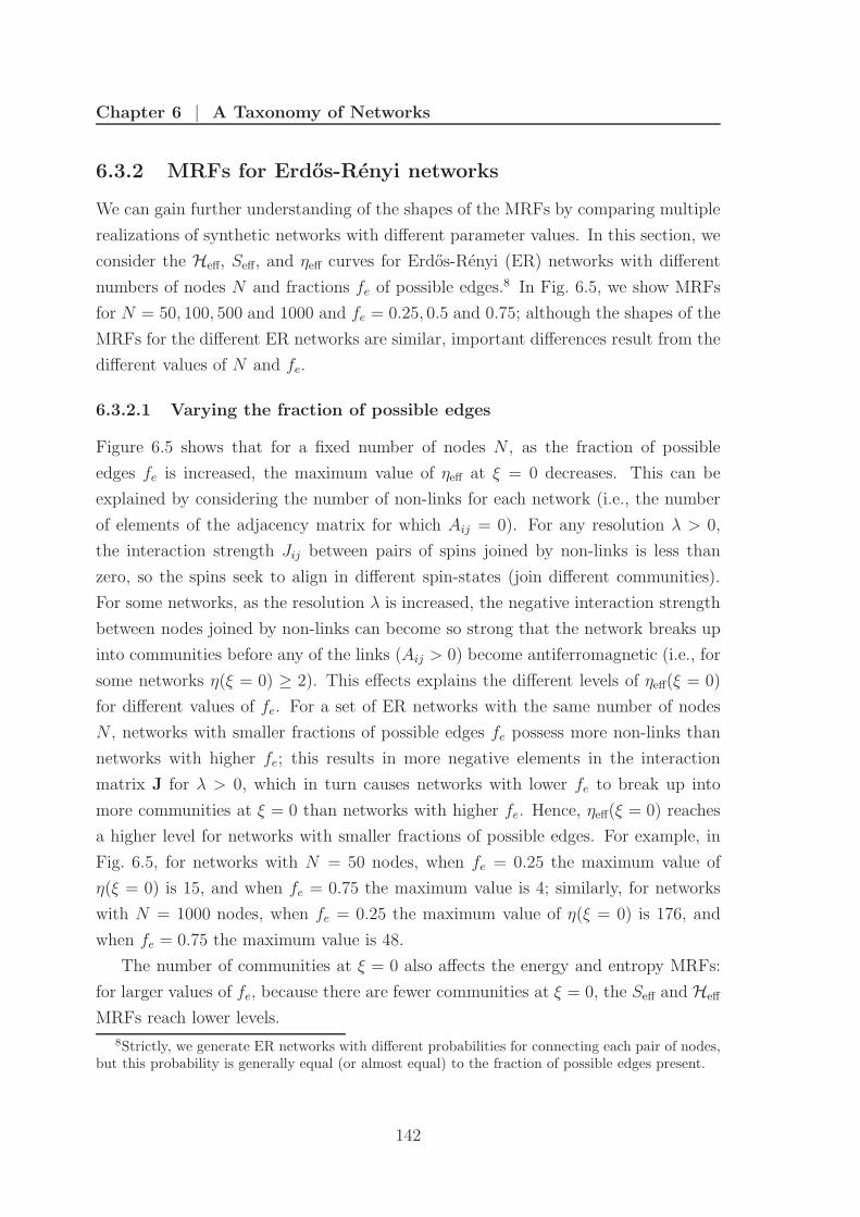
Chapter 6 | A Taxonomy of Networks
6.3.2 MRFs for Erdos-Renyi networks
We can gain further understanding of the shapes of the MRFs by comparing multiple
realizations of synthetic networks with different parameter values. In this section, we
consider the Heff, Seff, and ηeff curves for Erdos-Renyi (ER) networks with different
numbers of nodes N and fractions fe of possible edges.8 In Fig. 6.5, we show MRFs
for N = 50, 100, 500 and 1000 and fe = 0.25, 0.5 and 0.75; although the shapes of the
MRFs for the different ER networks are similar, important differences result from the
different values of N and fe.
6.3.2.1 Varying the fraction of possible edges
Figure 6.5 shows that for a fixed number of nodes N , as the fraction of possible
edges fe is increased, the maximum value of ηeff at ξ = 0 decreases. This can be
explained by considering the number of non-links for each network (i.e., the number
of elements of the adjacency matrix for which Aij = 0). For any resolution λ > 0,
the interaction strength Jij between pairs of spins joined by non-links is less than
zero, so the spins seek to align in different spin-states (join different communities).
For some networks, as the resolution λ is increased, the negative interaction strength
between nodes joined by non-links can become so strong that the network breaks up
into communities before any of the links (Aij > 0) become antiferromagnetic (i.e., for
some networks η(ξ = 0) ≥ 2). This effects explains the different levels of ηeff(ξ = 0)
for different values of fe. For a set of ER networks with the same number of nodes
N , networks with smaller fractions of possible edges fe possess more non-links than
networks with higher fe; this results in more negative elements in the interaction
matrix J for λ > 0, which in turn causes networks with lower fe to break up into
more communities at ξ = 0 than networks with higher fe. Hence, ηeff(ξ = 0) reaches
a higher level for networks with smaller fractions of possible edges. For example, in
Fig. 6.5, for networks with N = 50 nodes, when fe = 0.25 the maximum value of
η(ξ = 0) is 15, and when fe = 0.75 the maximum value is 4; similarly, for networks
with N = 1000 nodes, when fe = 0.25 the maximum value of η(ξ = 0) is 176, and
when fe = 0.75 the maximum value is 48.
The number of communities at ξ = 0 also affects the energy and entropy MRFs:
for larger values of fe, because there are fewer communities at ξ = 0, the Seff and Heff
MRFs reach lower levels.
8Strictly, we generate ER networks with different probabilities for connecting each pair of nodes,but this probability is generally equal (or almost equal) to the fraction of possible edges present.
142

6.3 | Mesoscopic response functions
0
0.5
1N = 50
f e = 0
.25
N = 100 N = 500 N = 1000
0
0.5
1
f e = 0
.5
0 0.5 1 0
0.5
1
f e = 0
.75
0 0.5 1 ξ
0 0.5 1 0 0.5 1
Heff
Seff
ηeff
Figure 6.5: A comparison of the Heff, Seff, and ηeff MRFs for Erdos-Renyi networkswith different numbers of nodes N and fractions of possible edges fe.
6.3.2.2 Varying the number of nodes
Figure 6.5 also shows that as the number of nodes increases, for the same fraction of
possible edges, the maximum value of ηeff at ξ = 0 decreases. For larger values of N ,
the network breaks up into more communities at ξ = 0 than for smaller N ; however,
the number of communities as a fraction of the number of nodes in the network is
lower, hence ηeff(ξ = 0) is lower. For example, for networks with fe = 0.25, when
N = 50 the maximum value of η(ξ = 0) is 15, which corresponds to η/N = 0.3, and
when N = 1000 the maximum value is 176, which corresponds to η/N = 0.18.
In contrast to the ηeff MRFs, for larger values of N at the same value of fe Seff
reaches a higher value at ξ = 0. The entropy can be considered as the uncertainty in
the community membership of a particular node. For a larger number of communities
there is generally greater uncertainty in the community membership of a randonly
chosen node, which results in a higher entropy and is consistent with the observation
that Seff(ξ = 0) is higher for larger N . However, because we normalize the entropy
using the transformation Seff = (S − Smin)/(Smax − Smin) = S/ log N (see Eq. 6.7),
more precisely, the higher value of Seff at ξ = 0 for higher N indicates that there is
greater uncertainty in the community membership of a node relative to the maximum
possible uncertainty (which occurs when all nodes are in singleton communities and
is given by Smax = log N).
143

Chapter 6 | A Taxonomy of Networks
Finally, Fig. 6.5 shows that for larger N the maximum value of Heff at ξ = 0
is higher. This is again explained in part by the fact that networks with larger
numbers of nodes fragment into more communities at ξ = 0 than smaller net-
works. Recall from Eq. 4.3 that the Hamiltonian of the Potts spin glass is given
by H =∑
i6=j Jijδ(Ci, Cj) = −∑i6=j (Aij − λPij) δ(Ci, Cj). The Kronecker delta
δ(Ci, Cj) means that the interaction energies Jij = (Aij − λPij) are only summed
over nodes that belong to the same community. Therefore, as the networks fragment,
the summation includes fewer terms so H becomes progressively less negative and
Heff increases. The higher values Heff at ξ = 0 for networks with more nodes can be
further explained by considering the distribution of Λij for the different networks. In
Fig. 6.6, we show that for larger N the distribution of Λij values is concentrated in a
sharper peak, which means that the resolution λ only needs to be swept over a small
range of values for all of the links to become antiferromagnetic. The small range of λ
also means that there is a relatively small change in energy as the network breaks up
into N communities, which explains the small difference in energy that we observe
between ξ = 0 and ξ = 1 in the Heff MRFs for larger networks in Fig. 6.5.
2 4 6 8 100
0.1
0.2ER: (500,25)
2 4 6 8 100
0.1
0.2ER: (1000,25)
1 2 3 40
0.1
0.2ER: (500,50)
1 2 3 40
0.1
0.2ER: (1000,50)
1 1.5 20
0.1
0.2ER: (500,75)
1 1.5 20
0.1
0.2ER: (1000,75)
2 4 6 8 100
0.1
0.2ER: (50,25)
2 4 6 8 100
0.1
0.2ER: (100,25)
1 2 3 40
0.1
0.2ER: (50,50)
norm
aliz
ed fr
eque
ncy
1 2 3 40
0.1
0.2ER: (100,50)
1 1.5 20
0.1
0.2ER: (50,75)
1 1.5 20
0.1
0.2ER: (100,75)
Λij
Figure 6.6: A comparison of the distribution of Λij values for Erdos-Renyi networkswith different numbers of nodes N and fractions of possible edges fe.
144

6.3 | Mesoscopic response functions
6.3.3 Synthetic MRFs
The shapes of the MRFs reflect the manner in which the network splits into commu-
nities as the resolution is increased. To provide further insights into the mesoscopic
heterogeneities leading to different MRFs it is therefore instructive to consider the ef-
fect of different community fragmentation mechanisms on the MRFs. In this section,
we do not assume any network structure or detect communities; instead, we create
synthetic ηeff and Seff MRFs by considering different rates of community fragmenta-
tion as a function of ξ and different community size distributions.
We begin by assuming a fixed shape for the ηeff response function. Figure 6.4
suggests that most of the ηeff curves are either approximately linear or some convex
function so, as a first approximation, we assume that the ηeff MRFs are either linear,
quadratic, or cubic.9 We create synthetic ηeff MRFs for each of these cases as follows.
We assume that as the resolution λ is increased, the number of communities increases
as
η(i) =
⌈
ik
Nk−1
⌉
, (6.9)
where ⌈x⌉ = minj ∈ Z|j ≥ x, with j denoting an integer, is the ceiling function, i ∈1, . . . , N, N is the number of nodes in the network and we investigate k ∈ 1, 2, 3.The normalization Nk−1 ensures that the number of communities does not exceed N
and the ceiling function ensures that we have only integer numbers of communities.
We normalize these values to effective numbers of communities ηeff lying in the unit
interval through the transformation
ηeff(i) =η(i) − ηmin
ηmax − ηmin=
η(i) − 1
N − 1. (6.10)
We then construct synthetic Seff MRFs based on the number of communities η at
each value of i in the ηeff MRFs. We investigate two extreme cases for the community
fragmentation process:
1. We consider the case in which each increase in the number of communities
η results from a single node leaving the largest community. For example, at
η = 2 we assume that one community contains a single node and the other
community contains N − 1 nodes; at η = 3, we assume that there are two
communities containing single nodes and a third community containing N − 2
nodes; and so on.
9Although this assumption is not strictly true for most networks, it is nevertheless a reasonablestarting point.
145

Chapter 6 | A Taxonomy of Networks
2. We examine the case in which each increase in η results from the largest com-
munity splitting in half. For example, at η = 2 we assume that each community
contains N/2 nodes; at η = 3, we assume that there are two communities con-
taining N/4 nodes and a third community containing N/2 nodes; at η = 4, we
assume that each community contains N/4 nodes; and so on.10
To plot the MRFs we assume that the ξ are uniformly distributed over the interval
[0, 1] such that the ith value is given by
ξ(i) =i − 1
N − 1, (6.11)
where i = 1, . . . , N . We show in Section 6.3.1 that the number of communities
increases to η > 1 at ξ = 0 for many networks, so for each splitting regime we
examine two behaviours for the MRFs at ξ = 0:
1. The number of communities does not exceed η = 1 at ξ = 0. (See columns A
and C in Fig. 6.7.)
2. The number of communities initially increases without an increase in the ef-
fective fraction of antiferromagnetic interactions ξ , i.e., η > 1 at ξ = 0. (See
columns B and D in Fig. 6.7.)
We create MRFs that represent the second type of behaviour by setting the first ι
elements of the ξ vector to zero; increasing ι results in the MRFs reaching a higher
values at ξ = 0.
In Fig. 6.7, we show synthetic MRFs for networks with N = 500 nodes and
ι = 20.11 For all of the curves where we assume that each increase in η results
from a single node leaving the largest community, the Seff MRF closely tracks the ηeff
MRF. For each example in which increases in η result from the largest community
splitting in half, the entropy increases faster than in the equivalent MRF for single
nodes splitting from the largest community. This is because in the former case there
is greater uncertainty in the community membership of individual nodes. Figure 6.7
also demonstrates that for the fragmentation mechanism in which communities split in
10When splitting the kth community into two, if nk/2 is not an integer (where nk is the numberof nodes in the kth community), we assume that one of the communities contains ⌊nk/2⌋ nodes andthat the other community contains ⌈nk/2⌉ nodes. If two communities contain the same number ofnodes, we choose one at random to split – this choice has no effect on the resulting MRF.
11We have also investigated networks with different numbers of nodes N and observe similardifferences in the MRFs for different sized networks to those described in Section 6.3.2 for ERnetworks.
146

6.3 | Mesoscopic response functions
half the MRFs have very different shapes for the different assumptions. For example,
there is a plateau in some, but not all, of the Seff MRFs and there is a large variation
in the amount by which the Seff MRFs increase at ξ = 0.
This is just a simple demonstration of how different fragmentation processes lead
to different shaped MRFs. For real-world networks, the community splitting mech-
anism is likely to be somewhere between these two extreme cases, with single nodes
leaving communities for some changes in ξ and communities splitting more equally
at other values.
0
0.5
1
linea
r
A B
0
0.5
1
quad
ratic
0 0.5 10
0.5
1
cubi
c
0 0.5 1ξ
C D
0 0.5 1 0 0.5 1
ηeff
Seff
Figure 6.7: Synthetic MRFs for ηeff and Seff. We assume that the ηeff responsefunctions are either linear, quadratic, or cubic. We also consider that: (A) Eachincrease in the number of communities η results from a single node leaving the largestcommunity. (B) Again, each increase in η results from a single node leaving thelargest community, but we make the additional assumption that, as the resolution isincreased, η initially increases without there being an increase in the effective numberof antiferromagnetic interactions ξ. (C) Each increase in the number of communities ηresults from the largest community splitting in half. (D) Each increase in the numberof communities η results from the largest community splitting in half and there isan initial increase in η without an increase in ξ. We assume that each network hasN = 500 nodes.
147

Chapter 6 | A Taxonomy of Networks
6.4 Distance measures
In Section 6.3, we demonstrated that there are significant variations in the shapes of
the MRFs for different networks. This variety reflects the diverse range of possible
mesoscopic network structures; if two networks have similar MRFs, this suggests that
the networks have similar mesoscopic properties. We now define a distance measure
that quantifies the differences in the behaviours of the MRFs.
There are several plausible choices of distance measure, but we add the constraint
that the measure should compare MRFs across all network scales (i.e., for all values of
ξ). With this in mind, we define the pairwise distance between networks with respect
to one of the investigated properties as the area between the corresponding MRFs.
For example, the distance between two networks i and j with respect to the effective
energy MRF Heff is given by
dHij =
∫ 1
0
|Hieff −Hj
eff|dξ. (6.12)
Similarly, for the effective entropy and effective number of communities, the distances
are given by
dSij =
∫ 1
0
|Sieff − Sj
eff|dξ (6.13)
and
dηij =
∫ 1
0
|ηieff − ηj
eff|dξ. (6.14)
We represent the three distances in matrix form as DH, DS, and Dη. This definition
of distance between MRFs has several desirable properties. First, as required, it
compares MRFs across all network scales (i.e., for all values of ξ); second, the measure
is bounded between 0 and 1; third, it is simple and transparent, in that the distances
correspond to the geometric area between a pair of MRFs; finally, we find a posteriori
that it seems to cluster networks accurately. We illustrate the distance measures in
Fig. 6.8 using the NYSE: 1984–1987 [229] and Fungal: (4,8) networks [33,113,114,288].
We analyze MRFs for the energy H, entropy S, and number of communities η, but
the techniques that we present work similarly for other summary statistics. However,
if two statistics provide very similar information, then one of them can be excluded
without a significant loss of information. We check whether the summary statistics
that we investigate are sufficiently different for it to be worthwhile to include all
of them in our analysis by calculating the correlation between their distance mea-
sures. In Fig. 6.9, we show scatter density plots for each pairwise combination of the
148
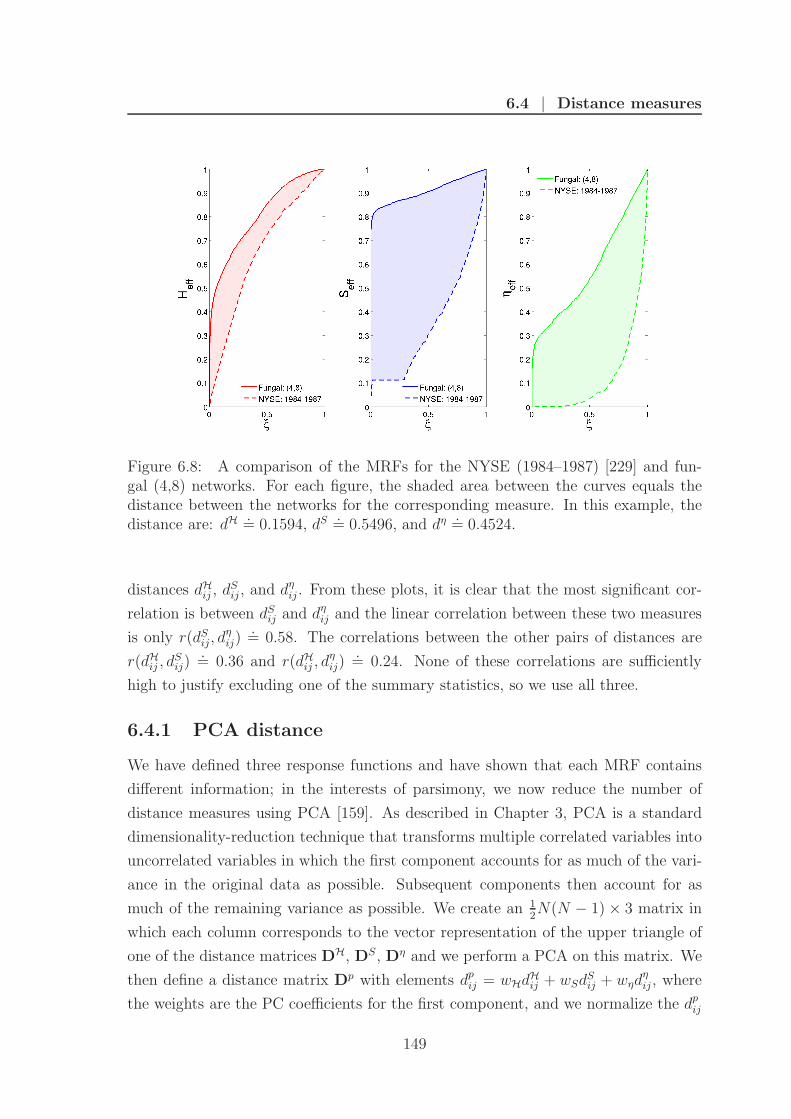
6.4 | Distance measures
Figure 6.8: A comparison of the MRFs for the NYSE (1984–1987) [229] and fun-gal (4,8) networks. For each figure, the shaded area between the curves equals thedistance between the networks for the corresponding measure. In this example, thedistance are: dH .
= 0.1594, dS .= 0.5496, and dη .
= 0.4524.
distances dHij , dS
ij , and dηij . From these plots, it is clear that the most significant cor-
relation is between dSij and dη
ij and the linear correlation between these two measures
is only r(dSij, d
ηij)
.= 0.58. The correlations between the other pairs of distances are
r(dHij , d
Sij)
.= 0.36 and r(dH
ij , dηij)
.= 0.24. None of these correlations are sufficiently
high to justify excluding one of the summary statistics, so we use all three.
6.4.1 PCA distance
We have defined three response functions and have shown that each MRF contains
different information; in the interests of parsimony, we now reduce the number of
distance measures using PCA [159]. As described in Chapter 3, PCA is a standard
dimensionality-reduction technique that transforms multiple correlated variables into
uncorrelated variables in which the first component accounts for as much of the vari-
ance in the original data as possible. Subsequent components then account for as
much of the remaining variance as possible. We create an 12N(N − 1) × 3 matrix in
which each column corresponds to the vector representation of the upper triangle of
one of the distance matrices DH, DS, Dη and we perform a PCA on this matrix. We
then define a distance matrix Dp with elements dpij = wHdH
ij + wSdSij + wηd
ηij , where
the weights are the PC coefficients for the first component, and we normalize the dpij
149

Chapter 6 | A Taxonomy of Networks
0 0.2 0.4 0.6 0.80
0.2
0.4
0.6
0.8
dS
dH
0 0.2 0.4 0.6 0.80
0.2
0.4
0.6
0.8
dSdη
0 0.2 0.4 0.6 0.80
0.2
0.4
0.6
0.8
dH
dη
Figure 6.9: Scatter density plots showing the correlation between the distancesmeasures dH
ij , dSij, and dη
ij. The linear correlations r between the distances are:r(dH
ij , dSij)
.= 0.36, r(dS
ij, dηij)
.= 0.58, and r(dH
ij , dηij)
.= 0.24.
to the unit interval. The PC coefficients are wH.= 0.24, wS
.= 0.79, and wη
.= 0.57.
The first component accounts for 69% of the variance of the system, so the distances
Dp provide a reasonable single-variable representation of the distances DH, DS, and
Dη.
6.4.2 Distance matrices
In Fig. 6.10, we show the distribution of distances for all of the 714 networks studied
(see Table C.1 for the full list of networks). The distribution dSij for the entropy
MRF has more weight at larger distances than the dHij and dη
ij distributions, which
suggests that the entropy MRFs distinguish the networks slightly better then the
other response functions. This is reflected in the fact that the weight wS is larger
than wH and wη.
In Fig. 6.11, we show the distance matrices DH, DS, Dη, and Dp. We have
block-diagonalized the distance matrices by reordering the nodes to maximize the
cost function
Φ =1
N
N∑
i,j=1
Xij |i − j|, (6.15)
which weights each matrix element with its distance to the diagonal (X ∈ dH, dS, dη, dp).Figure 6.11 also suggests that the distance dS
ij better separates the networks than the
distances dHij and dη
ij and it appears from this figure that dSij might separate the net-
works better than the PCA distance dpij. However, we demonstrate in Section 6.5.4
that this is not the case: the PCA distance dpij provides the best measure that we
have investigated for separating the networks into categories.
150

6.5 | Clustering networks
0 0.2 0.4 0.6 0.8 10
0.02
0.04
0.06
0.08
0.1
dH
norm
aliz
ed fr
eque
ncy
0 0.2 0.4 0.6 0.8 10
0.02
0.04
0.06
0.08
0.1
dS
norm
aliz
ed fr
eque
ncy
0 0.2 0.4 0.6 0.8 10
0.02
0.04
0.06
0.08
0.1
dη
norm
aliz
ed fr
eque
ncy
0 0.2 0.4 0.6 0.8 10
0.02
0.04
0.06
dp
norm
aliz
ed fr
eque
ncy
Figure 6.10: Distributions of the distances dHij , dS
ij , dηij, and dp
ij.
The block structure of the distance matrices in Fig. 6.11 suggests the existence
of different clusters of networks. However, for these clusters to be meaningful it is
important that the distance measures we define for comparing networks are robust
to small perturbations in network structure. Because many networks are obtained
empirically, it is expected that the network data will contain false positive and nega-
tive links; that is, there will be links erroneously included in the network that do not
exist, and links that do actually exist will be erroneously omitted from the network.
To test the robustness of our distance measures with respect to such false posi-
tive and negatives, we recalculate the MRFs for a subset of unweighted networks in
which some percentage of the links have been rewired. We investigate two rewiring
mechanisms: one in which the degree distribution and connectivity of each network
is maintained and another in which only the connectivity is maintained. We provide
details of the analysis of the sensitivity of the distance measures to false positive and
negative links in Appendix E. We find in both cases that the block structure in the
distance matrices is robust to random perturbations of the networks. This implies
that the MRF distance measures we define in Section 6.4 are robust and can be used
to identify networks with similar mesoscopic structures across multiple scales.
6.5 Clustering networks
We now use the distance matrices DH, DS, Dη, and Dp to cluster networks. Before
presenting network taxonomies, we provide some additional details that we use to
151

Chapter 6 | A Taxonomy of Networks
DH
0.1
0.2
0.3
0.4
0.5
DS
0.1
0.2
0.3
0.4
0.5
0.6
Dη
0
0.1
0.2
0.3
0.4
0.5
0.6
0.7
0.8
Dp
0
0.2
0.4
0.6
0.8
1
Figure 6.11: Block-diagonalized distance matrices DH, DS, Dη, and Dp.
152

6.5 | Clustering networks
study the clusters.
6.5.1 Network categories
We assign each of the networks to a family group that describes the type of network
(see Table 6.1). One of the primary reasons for assigning each network to a category
is to use this external categorization to help assess the quality of the taxonomy that is
produced by the unsupervised MRF clustering. The assignment of the networks to one
of these groups is subjective because several of the networks could belong to more than
one category. For example, one could categorize the network of hyperlinks between
blogs on U.S. politics [3] as a WWW network or a citation network, and one could
categorize the network of jazz musicians [125] as a collaboration network or a social
network. The initial selection of network categories is of course then also subjective.
One could argue that if one has a social network category, then it is not necessary
to have a collaboration network category as well because collaboration networks are
merely a subset of social networks. However, in choosing the network categories, we
have attempted to maintain a balance between having enough categories to make
it possible to understand the differences that lead to the network clusters without
having so many categories that it is impossible to discern the essential differences.
6.5.2 Selecting a subset of networks
We analyze a total of 714 networks (see Table C.1 for the full list); because of the
data that is available, the networks are not evenly distributed across categories (see
Table 6.1). Many of these networks are either different time-snapshots of the same net-
work or different realizations of the same type of network.12 For example, we include
110 roll-call voting networks for different sessions of the U.S. House of Representa-
tives [203,241,306] and 100 Facebook networks for different U.S. universities [295]. In
some of the analysis we present, we only study a subset of networks to have a more
balanced set across different categories. One of the primary reasons for doing this is
to keep the dendrograms readable. However, it is also true that to understand where
a particular type of networks lies in the taxonomy it is often necessary only to include
a representative subset of networks of that type. Therefore, for some of the analysis,
we focus on a subset of 270 networks (which we highlight in Table C.1).
12We analyze intra-category taxonomies in Section 6.9.
153

Chapter 6 | A Taxonomy of Networks
Table 6.1: Network categories and the number of networks assigned to each category.See Table C.1 for the identities of the networks.
Category No. of networks
Synthetic 64Social 26Facebook 100Political: voting 285Political: cosponsorship 26Political: committee 16Protein interaction 22Metabolic 43Brain 12Fungal 12Financial 69Language 8Collaboration 8WWW 3Electronic circuit 3Citation 3Trade 3Other 11
154

6.5 | Clustering networks
6.5.3 Choosing a linkage clustering algorithm
For each distance measure, we construct a dendrogram for the subset of networks used
in Section 6.5.2 using linkage clustering. As described in Sections 4.3 and 5.6, linkage
clustering is an agglomerative hierarchical clustering technique [84, 244]. The three
most common linkage clustering algorithms are single, average, and complete linkage
clustering, which join clusters of objects based on the smallest, average, and largest
distance between objects in the clusters, respectively. We compare dendrograms con-
structed with the different linkage clustering algorithms using the cophenetic correla-
tion coefficient ζ . We define tij as the distance in the dendrogram between networks
i and j. For example, for a dendrogram constructed from the PCA-distance matrix
Dp with elements dpij using single-linkage clustering, the distance tij between a node
i in cluster C and a node j in cluster C′ is given by (see Eq. 5.9)
tij = dsing(C, C′) = mini∈Cj∈C′
dpij . (6.16)
Similarly, for a dendrogram constructed using average-linkage clustering the distance
tij is given by (see Eq. 5.10)
tij = dave(C, C′) =1
|C||C′|∑
i∈C
∑
j∈C′
dpij, (6.17)
and for complete-linkage clustering by
tij = dcomp(C, C′) = maxi∈Cj∈C′
dpij . (6.18)
The cophenetic correlation, which measures how well each dendrogram preserves the
pairwise distances between the networks, is defined as [276]
ζ =
∑
i<j
(
dpij − dp
)(
tij − t)
√
[
∑
i<j
(
dpij − dp
)2][
∑
i<j
(
tij − t)2]
, (6.19)
where dp is the mean of the distances dpij and t the mean value of the tij .
The cophenetic correlations for the different linkage clustering algorithms are:
ζsing.= 0.65, ζave
.= 0.78, and ζcomp
.= 0.62. This implies that dendrograms con-
structed using average linkage clustering preserve the distances in Dp better than
those constructed using the other clustering techniques, so we use average linkage
clustering to construct all dendrograms in the remainder of this chapter.
155
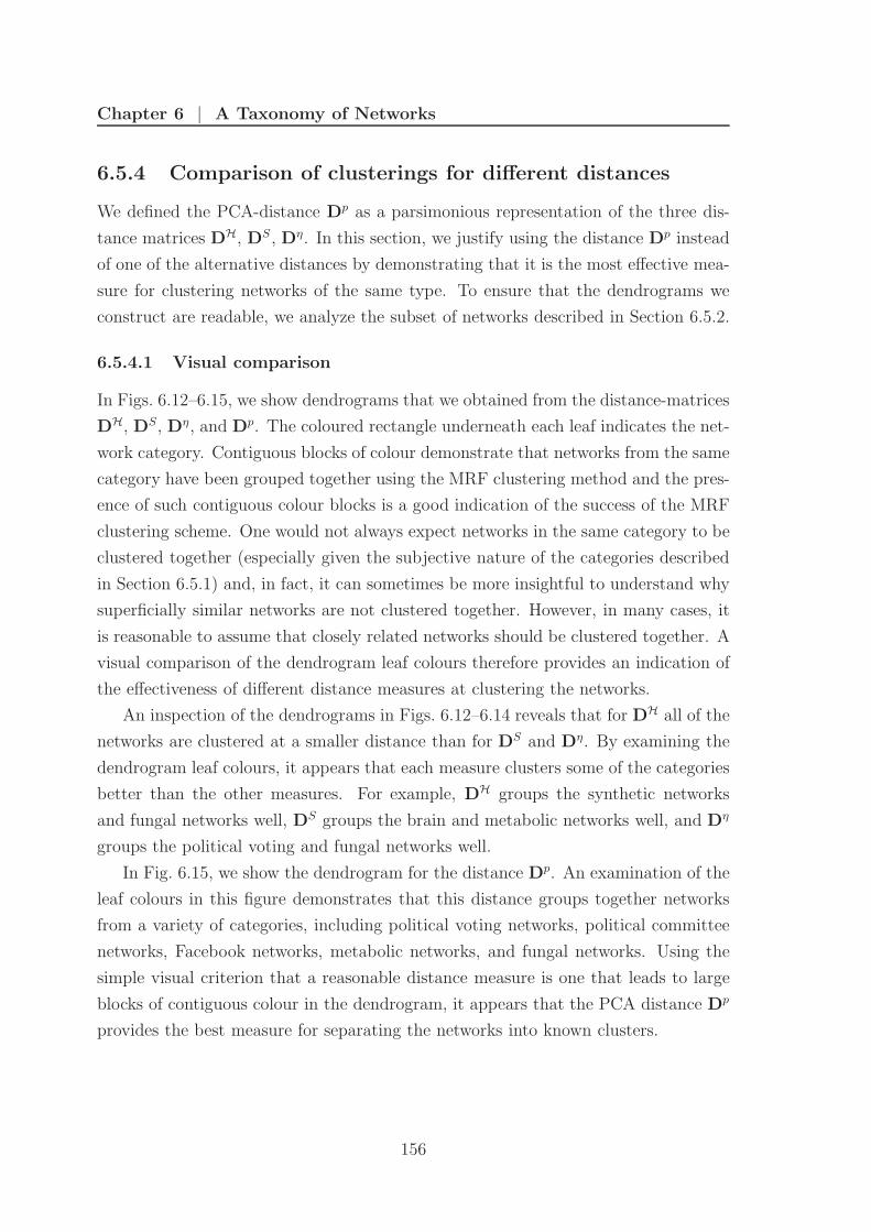
Chapter 6 | A Taxonomy of Networks
6.5.4 Comparison of clusterings for different distances
We defined the PCA-distance Dp as a parsimonious representation of the three dis-
tance matrices DH, DS, Dη. In this section, we justify using the distance Dp instead
of one of the alternative distances by demonstrating that it is the most effective mea-
sure for clustering networks of the same type. To ensure that the dendrograms we
construct are readable, we analyze the subset of networks described in Section 6.5.2.
6.5.4.1 Visual comparison
In Figs. 6.12–6.15, we show dendrograms that we obtained from the distance-matrices
DH, DS, Dη, and Dp. The coloured rectangle underneath each leaf indicates the net-
work category. Contiguous blocks of colour demonstrate that networks from the same
category have been grouped together using the MRF clustering method and the pres-
ence of such contiguous colour blocks is a good indication of the success of the MRF
clustering scheme. One would not always expect networks in the same category to be
clustered together (especially given the subjective nature of the categories described
in Section 6.5.1) and, in fact, it can sometimes be more insightful to understand why
superficially similar networks are not clustered together. However, in many cases, it
is reasonable to assume that closely related networks should be clustered together. A
visual comparison of the dendrogram leaf colours therefore provides an indication of
the effectiveness of different distance measures at clustering the networks.
An inspection of the dendrograms in Figs. 6.12–6.14 reveals that for DH all of the
networks are clustered at a smaller distance than for DS and Dη. By examining the
dendrogram leaf colours, it appears that each measure clusters some of the categories
better than the other measures. For example, DH groups the synthetic networks
and fungal networks well, DS groups the brain and metabolic networks well, and Dη
groups the political voting and fungal networks well.
In Fig. 6.15, we show the dendrogram for the distance Dp. An examination of the
leaf colours in this figure demonstrates that this distance groups together networks
from a variety of categories, including political voting networks, political committee
networks, Facebook networks, metabolic networks, and fungal networks. Using the
simple visual criterion that a reasonable distance measure is one that leads to large
blocks of contiguous colour in the dendrogram, it appears that the PCA distance Dp
provides the best measure for separating the networks into known clusters.
156
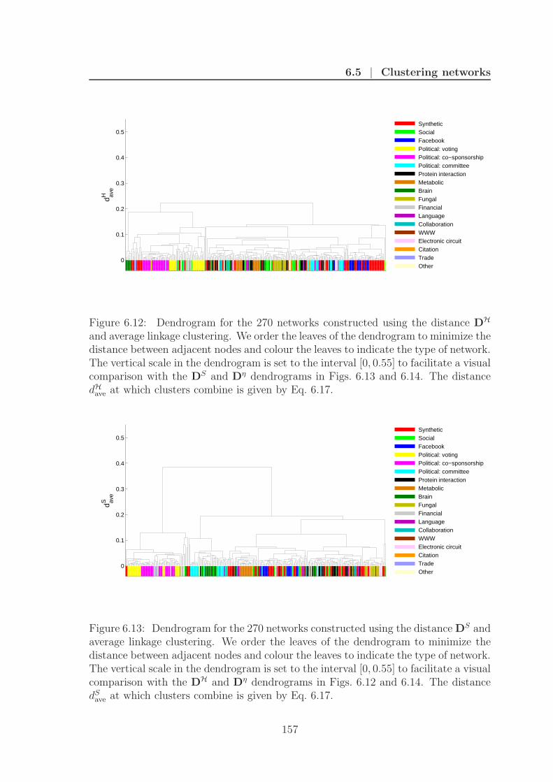
6.5 | Clustering networks
0
0.1
0.2
0.3
0.4
0.5
d ave
H
SyntheticSocialFacebookPolitical: votingPolitical: co−sponsorshipPolitical: committeeProtein interactionMetabolicBrainFungalFinancialLanguageCollaborationWWWElectronic circuitCitationTradeOther
Figure 6.12: Dendrogram for the 270 networks constructed using the distance DH
and average linkage clustering. We order the leaves of the dendrogram to minimize thedistance between adjacent nodes and colour the leaves to indicate the type of network.The vertical scale in the dendrogram is set to the interval [0, 0.55] to facilitate a visualcomparison with the DS and Dη dendrograms in Figs. 6.13 and 6.14. The distancedH
ave at which clusters combine is given by Eq. 6.17.
0
0.1
0.2
0.3
0.4
0.5
d ave
S
SyntheticSocialFacebookPolitical: votingPolitical: co−sponsorshipPolitical: committeeProtein interactionMetabolicBrainFungalFinancialLanguageCollaborationWWWElectronic circuitCitationTradeOther
Figure 6.13: Dendrogram for the 270 networks constructed using the distance DS andaverage linkage clustering. We order the leaves of the dendrogram to minimize thedistance between adjacent nodes and colour the leaves to indicate the type of network.The vertical scale in the dendrogram is set to the interval [0, 0.55] to facilitate a visualcomparison with the DH and Dη dendrograms in Figs. 6.12 and 6.14. The distancedS
ave at which clusters combine is given by Eq. 6.17.
157

Chapter 6 | A Taxonomy of Networks
0
0.1
0.2
0.3
0.4
0.5
d ave
η
SyntheticSocialFacebookPolitical: votingPolitical: co−sponsorshipPolitical: committeeProtein interactionMetabolicBrainFungalFinancialLanguageCollaborationWWWElectronic circuitCitationTradeOther
Figure 6.14: Dendrogram for the 270 networks constructed using the distance Dη andaverage linkage clustering. We order the leaves of the dendrogram to minimize thedistance between adjacent nodes and colour the leaves to indicate the type of network.The vertical scale in the dendrogram is set to the interval [0, 0.55] to facilitate a visualcomparison with the DH and DS dendrograms in Figs. 6.12 and 6.13. The distancedη
ave at which clusters combine is given by Eq. 6.17.
6.5.4.2 Metric comparison
A visual comparison is a good starting point for assessing the effectiveness of differ-
ent distance measures at clustering networks, but it is a subjective assessment. We
therefore introduce a metric to quantify how effectively each distance measure clusters
networks of the same type.
The assignment of networks to family categories is also subjective and some of
the categories include networks of very different types (see Section 6.5.1), so it is
inappropriate to assess the effectiveness of a distance measure based on how well it
clusters all types of networks. Instead, we focus only on groups of networks that are
clustered together in any one of the dendrograms in Figs. 6.12–6.15. This includes
the following 8 categories: Facebook, metabolic, political co-sponsorship, political
committee, political voting, financial, brain, and fungal networks.
For each distance measure, we construct a dendrogram and for each level of the
dendrogram we calculate the maximum fraction of networks of a particular type that
appear in the same cluster. That is, for a particular level of the dendrogram, we
take a network category and find all clusters that contain at least one network from
that category. We then calculate the fraction of networks from that category in each
158

6.5
|C
luste
ring
netw
ork
s
0
0.1
0.2
0.3
0.4
0.5
d ave
p
SyntheticSocialFacebookPolitical: votingPolitical: co−sponsorshipPolitical: committeeProtein interactionMetabolicBrainFungalFinancialLanguageCollaborationWWWElectronic circuitCitationTradeOther
Figure 6.15: Dendrogram for the 270 networks constructed using the distance Dp and average linkage clustering. We orderthe leaves of the dendrogram to minimize the distance between adjacent nodes and colour the leaves to indicate the type ofnetwork. A visual comparison with the DH, DS, and Dη dendrograms in Figs. 6.12, 6.13, and 6.14 shows that the distancematrix Dp provides a better separation of the networks into their groups. The distance dp
ave at which clusters combine is givenby Eq. 6.17.
159
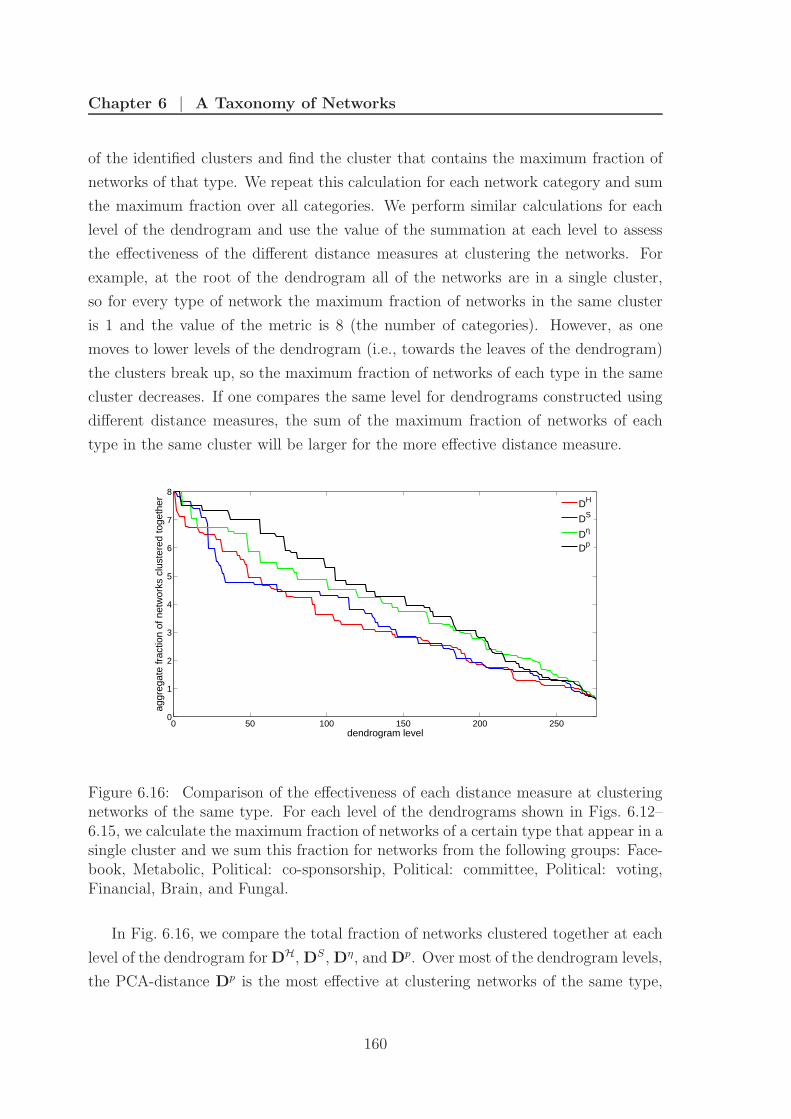
Chapter 6 | A Taxonomy of Networks
of the identified clusters and find the cluster that contains the maximum fraction of
networks of that type. We repeat this calculation for each network category and sum
the maximum fraction over all categories. We perform similar calculations for each
level of the dendrogram and use the value of the summation at each level to assess
the effectiveness of the different distance measures at clustering the networks. For
example, at the root of the dendrogram all of the networks are in a single cluster,
so for every type of network the maximum fraction of networks in the same cluster
is 1 and the value of the metric is 8 (the number of categories). However, as one
moves to lower levels of the dendrogram (i.e., towards the leaves of the dendrogram)
the clusters break up, so the maximum fraction of networks of each type in the same
cluster decreases. If one compares the same level for dendrograms constructed using
different distance measures, the sum of the maximum fraction of networks of each
type in the same cluster will be larger for the more effective distance measure.
0 50 100 150 200 2500
1
2
3
4
5
6
7
8
dendrogram level
aggr
egat
e fr
actio
n of
net
wor
ks c
lust
ered
toge
ther
DH
DS
Dη
Dp
Figure 6.16: Comparison of the effectiveness of each distance measure at clusteringnetworks of the same type. For each level of the dendrograms shown in Figs. 6.12–6.15, we calculate the maximum fraction of networks of a certain type that appear in asingle cluster and we sum this fraction for networks from the following groups: Face-book, Metabolic, Political: co-sponsorship, Political: committee, Political: voting,Financial, Brain, and Fungal.
In Fig. 6.16, we compare the total fraction of networks clustered together at each
level of the dendrogram for DH, DS, Dη, and Dp. Over most of the dendrogram levels,
the PCA-distance Dp is the most effective at clustering networks of the same type,
160
6.6 | Network taxonomies
which agrees with our visual assessment of the different distances in Section 6.5.4.1.13
We therefore focus on PCA-distance dendrograms for the remainder of this chapter.
6.6 Network taxonomies
6.6.1 Taxonomy of all networks
As we noted in Section 6.5.1, there is some subjectivity in selecting categories of
networks and assigning networks to these categories. However, for many of the studied
networks the category assignment is unequivocal, so it is insightful to consider how
networks within categories are distributed across the branches of the dendrogram.
In Fig. 6.17 we show a dendrogram containing leaves for all of the 714 networks
studied. In this dendrogram, there are several large contiguous blocks of leaves that
correspond to networks belonging to the same category. For example, there are
large contiguous blocks of fungal, Facebook, metabolic, political committee, political
voting, and financial networks. These blocks do not always include all of the networks
within a category; when there are separate contiguous blocks for the same category,
the blocks sometimes correspond to different types of networks within a category. For
example, there are separate blocks of FX networks and New York Stock Exchange
networks for the financial networks category. However, because of the number of
networks that we include in the study and the imbalance in the spread of networks
across categories, Fig. 6.17 is quite difficult to interpret and the smaller categories are
obfuscated by the larger categories. Therefore, for a clearer view of the relationships
between the different categories of networks, we return to considering the dendrogram
in Fig. 6.15 for the subset of 270 networks.
6.6.2 Taxonomy of a sub-set of networks
In the dendrogram in Fig. 6.15 all of the networks in some categories appear in
blocks of adjacent leaves. For example, there is a cluster of political voting networks
at the far left of the dendrogram. This cluster includes voting networks from the U.S.
Senate, the U.S. House of Representatives, the U.K. House of Commons, and the
13Figure 6.16 shows that at the highest and lowest levels of the dendrogram the PCA distancedoes not have the largest value of the metric used to assess the effectiveness of the different distances.These extreme levels correspond to most nodes in individual clusters and most nodes in the samecluster, respectively, and are not particularly insightful. The clusters that we observe over theintermediate levels of the dendrogram provide more insights into the relationships between thedifferent types of networks; over these intermediate dendrogram levels the PCA distance is the mosteffective at clustering the networks.
161

Chapte
r6
|A
Taxonom
yofN
etw
ork
s
0
0.05
0.1
0.15
0.2
0.25
0.3
0.35
0.4
d ave
p
Synthetic
Social
Political: voting
Political: co−sponsorship
Political: committee
Protein interaction
Metabolic
Brain
Fungal
Financial
Language
Collaboration
WWW
Electronic circuit
Citation
Trade
Other
Figure 6.17: Dendrogram for the 714 networks constructed using the distance Dp and average linkage clustering. We orderthe leaves of the dendrogram to minimize the distance between adjacent nodes and colour the leaves to indicate the type ofnetwork.
162

6.6 | Network taxonomies
United Nations General Assembly. The clustering of these voting networks suggests
that there are some common features in the MRFs that represent universal properties
of the different parliaments and legislatures. We also obtain single blocks that consist
of all political committee networks and all metabolic networks.
The political cosponsorship networks are split into two blocks that are separated by
a cluster of financial and trade networks. The leftmost block of political cosponsorship
networks consists of all of the House of Representatives cosponsorship networks, and
the rightmost cluster consists of all of the Senate cosponsorship networks. There are
also several categories for which all except one or two networks are clustered together
in a contiguous block. For example, all but two of the fungal networks appear in the
same block and all but one of the Facebook networks are clustered together. The
isolated Facebook network is the Caltech network (which is the smallest network of
this type), and it appears in a cluster next to the cluster containing all of the other
Facebook networks.
There are other categories of network that do not appear in near-contiguous blocks.
For example, protein interaction networks appear in several clusters. These networks
represent interactions within several different organisms, so one might not expect
all of them to be clustered together. However, there are also examples of protein
interaction networks for the same organism in which the interactions were identified
using different experimental techniques that are not clustered together. This supports
previous work that suggests that the properties of protein interaction networks are
extremely sensitive to the experimental procedure used to identify the interactions,
e.g., [145, 313].
Social networks are also distributed throughout the dendrogram. This is unsur-
prising given the extremely broad nature of the category: the social network category
includes networks of very different sizes with links representing a rather diverse range
of social interactions (see Table C.1 for details of the different networks). The leftmost
outlying social network is the network of Marvel comic book characters, which is ar-
guably not a typical social network. Finally, the synthetic networks appear in clusters
in different regions of the dendrogram, which is again unsurprising given that many
of these graphs were developed to model systems with very different characteristics.
It is also worth highlighting the initial split of the dendrogram into two clusters.
One of the clusters contains only three networks, whereas the other cluster contains
all of the other networks. This suggests that the three networks in the smaller cluster
possess unusual mesoscopic structures. The three networks are the NCAA football
163

Chapter 6 | A Taxonomy of Networks
schedule network [61] and two fractal networks [279]. The key feature that distin-
guishes these networks from most of the other networks are their degree distributions.
For each of the networks in the small cluster all of the nodes have one of a limited
number of possible degrees; for example, in the NCAA football networks, all but one
of the nodes have a degree of 12 or 13. Such degree distributions result in MRFs that
contain several plateaus (see Section 6.3.1) and lead to large distances between these
networks and the other networks in the taxonomy.
The observations in this section demonstrate that the MRF framework is able to
cluster categories of networks that are known to have similar structures, which verifies
the effectiveness of this technique. However, sometimes networks that one might
expect to be similar are not clustered together. These outliers might correspond to
anomalous members of a class of networks, so understanding the differences in their
structure is potentially insightful.
6.6.3 Taxonomy of network categories
In the previous sections, we applied the MRF clustering framework to individual net-
works. We now establish a taxonomy of network categories. We consider all empirical
network categories for which we have 8 or more networks.14 In Fig. 6.18, we show
the range of the Heff, Seff, and ηeff MRF curves for each category. Figure 6.18 demon-
strates that the MRFs for some classes of networks (such as political co-sponsorship
and metabolic networks) are very similar, whereas there are large variations in the
MRFs for other categories (such as social and protein interaction networks). The
range of different MRFs for the social and protein interactions explains why these
networks are scattered throughout the dendrogram in Fig. 6.15. Despite these differ-
ences, it instructive to create a taxonomy of network categories.
We compute average intra-class MRFs for each category by calculating the mean
of Heff, Seff, and ηeff over all networks within the category, and create a PCA-distance
matrix and taxonomy using the MRFs. At the highest level, the dendrogram in
Fig. 6.19 is split into two clear clusters. The lower of the two clusters contains finan-
cial, political voting, and political cosponsorship networks. All of these networks are
constructed from measures that characterize the similarity of nodes in the networks;
as this measure can be computed between any two nodes, these networks are typically
weighted and fully connected. The upper cluster contain all of the other categories.
The clear outlier in this cluster is the fungal networks, which are not closely related
14We do not consider synthetic networks because these networks are designed to model networkswith very different characteristics, so do not form a coherent category.
164

6.6 | Network taxonomies
to any of the other categories. This observation is unsurprising given the tree-like
structure of fungal networks [33]. The other categories of networks within this cluster
appear to be more closely related. For example, protein interaction networks cluster
with collaboration networks, Facebook networks cluster with language networks, and
metabolic networks cluster with social networks.
It is tempting to speculate on the reasons for these similarities, but the taxonomy
needs to be treated with some caution because of the differences in the intra-class
MRFs highlighted in Fig. 6.18. Nonetheless, Fig. 6.19 does suggest that networks
that are clustered together have some similarities in their mesoscopic structures; con-
sequently, a detailed comparison of the properties of networks from related categories
might help to identify common structures that support the functions of the differ-
ent types of networks. In addition, the taxonomy in Fig. 6.19 might also help to
identify network analysis techniques that might fruitfully be applied to a particular
network. For example, if biologists have developed techniques that provide insights
into protein interactions networks, the same techniques might successfully be applied
to collaboration networks.
Figure 6.18: MRFs for all of the network categories containing 8 or more networks(see Table 6.1). At each value of ξ, the upper curve shows the maximum value ofHeff, Seff, or ηeff for all networks in the category, the dashed curve shows the mean,and the lower curve shows the minimum value.
165

Chapter 6 | A Taxonomy of Networks
0.05 0.1 0.15 0.2 0.25 0.3 0.35 0.4 0.45 0.5 0.55
Political: co−sponsorship
Political: voting
Financial
Brain
Political: committee
Social
Metabolic
Language
Collaboration
Protein interaction
Fungal
davep
Figure 6.19: Taxonomy of network categories based on the average intra-class MRFs.The dendrogram is constructed using the distance Dp and average linkage clustering.We order the leaves of the dendrogram to minimize the distance between adjacentnodes
6.6.4 Comparison with prior clusterings
It is also worthwhile to compare the clusters that we identify with those found in the
prior studies of Milo et al. [210] and Guimera et al. [142] discussed in Section 4.5.
Such a comparison is difficult because, although we study many more networks, we
do not include all of the networks used in the other studies because they are not all
publicly available. Nevertheless, we can make some comparisons of the clusterings.
We cluster all but one of the language networks studied by Milo et al. in the same
cluster, but we study the undirected versions of these networks whereas Milo et al.
studied the directed networks.15 These networks are not clustered with other networks
in the language category, which are distributed throughout the dendrogram. However,
scrutiny of the language category in Table C.1 shows that the language networks
are constructed from very different sources, so it is unsurprising that they are not
clustered. We only include a single airline network but, in contrast to the study of
Guimera et al., this network is not clustered with the metabolic networks. In further
contrast to the work of Guimera et al., the MRF framework does not cluster all protein
interaction networks in the same cluster. Importantly, as stated above, we include
protein networks that have been derived using different experimental techniques, so
15The network that appears in a different cluster is the English word adjacency network [210].
166

6.6 | Network taxonomies
their appearance in different clusters is unsurprising.
We are only able to make a few comparisons of the different clustering frameworks
because of the differences in the networks used in each study. To perform a more
meaningful comparison it would be necessary to repeat the analyses of Refs. [210]
and [142] using a larger set of networks.
6.6.5 Synthetic networks
It is also insightful to consider the cluster membership of the synthetic networks.
The set of synthetic networks we study includes a wide range of networks models
and benchmark networks introduced to test community detection algorithms (see
Appendix C for a detailed description of the networks). An understanding of the
similarities between the MRFs for real and synthetic networks is important because
if a synthetic network has a similar MRF to a real-world network, the generative
mechanism used to produce the synthetic network might help in understanding the
structure of the real-world network.
In Fig. 6.20, we redraw the dendrogram in Fig. 6.15 with two colour bars under
each leaf: the upper bar indicates the network category and the lower bar indicates
the type of synthetic network. Figure 6.20 shows that the fractal networks are dis-
tributed throughout the dendrogram, whereas the other synthetic networks tend to
be localized in particular clusters. There is only one synthetic network in the left-
most cluster of the dendrogram, which contains weighted, fully-connected networks
constructed from similarity measures. We include random fully-connected networks
in the study but, despite having similar fractions of edges present, the MRFs of these
networks are not similar to those for real-world fully-connected networks. Many of
the synthetic networks lie in similar regions of the dendrogram. For example, there is
a group including LF benchmark, LFR benchmark, KOSKK model, ER, and H13-4
benchmark networks near the centre of the dendrogram. We study a wide range of
synthetic networks (and many of the most widely studied models), but we have not
included an exhaustive set and consequently we need to be careful not to make any
too strong statements based on the synthetic networks16. However, the absence of
any synthetic networks in many regions of the dendrograms suggests that, in terms
of mesoscopic structure, current network models are not representative of the full set
of real-world networks.
16Of course, this is also true of the real-world networks.
167

Chapter 6 | A Taxonomy of Networks
ERWSBAFractalRandom fully−connectedWeightedLFR benchmarkLF benchmarkH13−4 benchmarkLF−NG benhcmarkNon−synthetic
SyntheticSocialFacebookPolitical: votingPolitical: co−sponsorshipPolitical: committeeProtein interactionMetabolicBrainFungalFinancialLanguageCollaborationWWWElectronic circuitCitationTradeOther
Figure 6.20: Dendrogram for the 270 networks constructed using the distance dpij and
average linkage clustering. We order the leaves of the dendrogram to minimize thedistance between adjacent nodes. The upper colour bar indicates the type of networkand the lower colour bar shows all non-synthetic networks in grey and highlights theposition in the dendrogram of different types of synthetic network (see Appendix Cfor a description of the networks).
6.7 Clustering networks using other properties
Having established that the MRF framework produces a sensible clustering of net-
works, we now check that the observed taxonomy cannot be explained using simpler
summary statistics.
6.7.1 Simple network statistics
Perhaps the three simplest properties of an undirected network are whether it has
weighted or unweighted links, the number of nodes N , and the fraction of possible
edges that are present (which is given by 2L/[N(N − 1)]). In Fig. 6.21, we again
reproduce the dendrogram in Fig. 6.15 but now include a coloured bar under the
leaves for each of these properties. The top coloured row in Fig. 6.21 indicates that
many of the weighted networks are clustered together at the far left of the dendrogram.
However, there are also weighted networks scattered throughout the dendrogram, so
whether a network is weighted or unweighted does not explain the observed clustering.
The third coloured row provides a clearer explanation for the leftmost cluster: these
are not simply weighted networks, they are in fact weighted networks that contain all
168

6.7 | Clustering networks using other properties
weighted
unweighted
log(
frac
tion
of p
ossi
ble
edge
s)
−8.6
−7.6
−6.7
−5.7
−4.8
−3.8
−2.9
−1.9
−0.95
0.005
log(
num
ber
of n
odes
)
3.4
4.2
4.9
5.7
6.5
7.3
8
8.8
9.6
10
Figure 6.21: Dendrogram for the 270 networks constructed using the distance dpij and
average linkage clustering. We order the leaves of the dendrogram to minimize thedistance between adjacent nodes. The three colour bars below the dendrogram indi-cate (top): whether the network corresponding to each leaf is weighted or unweighted,(middle) the number of nodes in the networks, and (bottom) the fraction of possibleedges that are present. These colour bars clearly demonstrate that although someof the clustering in the dendrogram is attributable to these simple properties, theycannot explain much of the observed structure.
169

Chapter 6 | A Taxonomy of Networks
(or nearly all) possible edges17. Again, however, this property alone cannot explain
the observed clusters, as several of the weighted networks that possess nearly all
possible links do not appear in the leftmost cluster of the dendrogram. In fact,
there are many clusters in the dendrogram that contain networks with very different
fractions of possible edges. The third property we consider, the number of nodes,
again explains some of the clustering as networks with similar numbers of nodes
are clustered together in some regions of the dendrogram; however, there are also
numerous examples in which networks with the same number of nodes appear in
different clusters. Therefore, none of these simple network metrics can explain the
observed clustering.
6.7.2 Strength distribution
We also consider whether we can obtain a better taxonomy using microscopic network
properties. Of course, our original objective was to cluster networks based on their
mesoscopic structure, but it is nonetheless informative to compare the MRF clustering
with a clustering obtained using microscopic properties. The most widely studied
microscopic property is the vertex degree which has been found to follow a heavy-
tailed distribution in many empirically observed networks [9, 217]. Here we use the
strength distribution (i.e., the generalization of the degree distribution to weighted
networks) to compare networks. We denote the cumulative strength distribution of
the network i as Fi(k), which is the probability that the strength of a randomly
sampled node is greater than or equal to k. We then define the distance ddij between
the strength distributions of networks i and j as the Kolmogorov-Smirnov statistic [42]
ddij = sup
k
|Fi(k) − Fj(k)|, (6.20)
where sup denotes the supremum, and we represent these distances in matrix form
as Dd.
In Fig. 6.22, we show the dendrogram constructed using Dd. In Fig. 6.23, we use
the metric described in Section 6.5.4.2 to compare the effectiveness of Dd and the
PCA-distance Dp at clustering groups of networks belonging to the same category
(see Section 6.5.4.2). Figure 6.23 demonstrates that the PCA-distance performs better
than the strength distribution distance. In addition, the wealth of similar heights of
the branches in the dendrogram in Fig. 6.22 indicates that the strength distribution
17This cluster contains the networks constructed from similarity measures that we discussed inSections 6.6.5 and 6.6.3.
170

6.8 | Robustness of MRFs for different heuristics
clustering is not very robust because very slight methodological differences might lead
to large differences in the clusters.
0
0.1
0.2
0.3
0.4
0.5
0.6
0.7
0.8
0.9
1
d ave
d
SyntheticSocialFacebookPolitical: votingPolitical: co−sponsorshipPolitical: committeeProtein interactionMetabolicBrainFungalFinancialLanguageCollaborationWWWElectronic circuitCitationTradeOther
Figure 6.22: Dendrogram for the 270 networks constructed using the distance be-tween the strength distributions of the networks and average-linkage clustering. Weorder the leaves of the dendrogram to minimize the distance between adjacent nodesand colour them to indicate the type of network. The dendrogram demonstrates thatclustering using the strength distribution does not separate the networks into theirgroups as effectively as the distance matrix Dp that we obtained using MRFs. Thedistance dd
ave at which clusters combine is given by Eq. 6.17.
6.8 Robustness of MRFs for different heuristics
In this chapter we have detected all communities by minimizing the Hamiltonian in
Eq. 6.1 using a greedy algorithm [44]. However, as we noted in Sections 4.3.3 and
5.10, several alternative computational heuristics exist, so it is important to check
that the MRFs and taxonomies that we produce are robust with respect to the choice
of heuristic. In Appendix F, we provide a detailed analysis of the effects on the MRFs
and taxonomies of using spectral [221] and simulated annealing algorithms [141] to
minimize Eq. 6.1. We find small variations in the MRFs generated for the different
algorithms, but these differences have very little effect on the resulting dendrograms.
The taxonomies that we observe are therefore robust with respect to the choice of
optimization heuristic.
171

Chapter 6 | A Taxonomy of Networks
0 50 100 150 200 2500
1
2
3
4
5
6
7
8
dendrogram level
aggr
egat
e fr
actio
n of
net
wor
ks c
lust
ered
toge
ther
Dp
Dd
Figure 6.23: Comparison of the effectiveness of the PCA-distance Dp and the strengthdistribution distance Dd at clustering networks of the same type. For each level ofthe dendrograms shown in Figs. 6.15 and 6.22, we calculate the maximum fraction ofnetworks of a certain type that appear in a single cluster and we sum this fraction fornetworks from the following groups: Facebook, Metabolic, Political: co-sponsorship,Political: committee, Political: voting, Financial, Brain, and Fungal.
6.9 Case studies
Thus far, we have used the MRF framework to create taxonomies of large sets of
networks of different types. We now cluster individual families of networks in order
to demonstrate that our method can generate meaningful intra-class taxonomies.
We present a number of case studies in which we cluster groups of networks that
represent different time snapshots of the same system and groups of network that
represent multiple realizations of the same system. Networks in each of these families
could be studied using field-specific methods, but this approach would not make it
possible to relate different families to each other. By comparing the results of the
MRF framework with those obtained using methods specific to the relevant field we
can further verify that the MRF approach produces meaningful results.
6.9.1 U.S. Congressional roll-call voting
We first consider roll-call voting in the U.S. Congress, which is the legislative branch
of the U.S. federal government. Congress is formed of two chambers: the Senate
and the House of Representatives. The current Congress consists of 100 senators and
172
6.9 | Case studies
435 members of the House. We analyze roll-call voting for the 1st–110th Congresses,
covering the period 1789–2008. We construct networks from the roll call data [241] for
each two-year Congress as follows [306]. The roll calls for each chamber are encoded
in an N × b matrix M, in which each element Mik equals 1 if legislator i voted
yea on bill k, −1 if the legislator voted nay, and 0 otherwise. We are interested in
characterizing the similarities between legislators, so we transform M into an N ×N
adjacency matrix A with elements
Aij =1
bij
∑
k
αijk, (6.21)
where αijk = 1 if legislators i and j voted the same on bill k and 0 otherwise, and bij is
the total number of bills on which i and j both voted [243,306]. The elements Aii all
equal 1, indicating the perfect similarity between each legislator’s voting record with
himself/herself. We set all Aii = 0 to remove self-edges. The matrix A, with elements
Aij in the interval [0, 1], then represents a network of weighted ties between legislators,
where the weights are determined by the similarity of their roll-call voting over a single
two-year Congress. Following Ref. [241], we only consider “non-unanimous” roll call
votes, where a roll call vote is considered “non-unanimous” if more than 3% of the
legislators are in the minority.
6.9.1.1 Party polarization
For each Congress, we calculate MRFs for both the House and Senate and cluster
the Congresses for each chamber by comparing the MRFs. In Figs. 6.24(a) and
6.24(b), we show dendrograms for the House of Representatives and Senate, respec-
tively. Much work on the U.S. Congress has been devoted to the extent of partisan
polarization, the influence of party on roll-call voting, and the degree to which this
has varied over time (see Refs. [203, 306] and references therein). In highly-polarized
legislatures, representatives tend to vote along party lines, so there are strong simi-
larities in the voting patterns of members of the same party, and strong differences
between members of different parties. In contrast, during periods of low polarization,
the party lines become blurred and there are greater similarities in the voting patterns
of members of different parties.
We use the notion of party polarization to understand the taxonomy of Con-
gresses shown in Figs. 6.24(a) and 6.24(b). We consider two measures of polarization.
The first uses DW-Nominate scores, a multi-dimensional scaling technique that is
very popular among political scientists [203, 241]. The DW-Nominate polarization is
173

Chapter 6 | A Taxonomy of Networks
given by the absolute value of the difference between the mean first-dimension DW-
Nominate scores for members of one party and the same mean for members of the
other party (see Refs. [203, 241] for a detailed description of DW-Nominate scores).
The problem with the DW-Nominate polarization is that it assumes a competitive
two-party system and therefore cannot be calculated prior to the 46th Congress. The
second measure we consider is the modularity Q, which was recently shown to be a
good measure of polarization [306], even for Congresses without a clear division into
parties. Modularity is given, in terms of the energy H in Eq. 6.1 as
Q = −H(λ = 1)
2m. (6.22)
The two measures agree fairly closely on the level of polarization of each Congress for
which they can both be calculated, although there are some differences [306].
In Figs. 6.24(a) and 6.24(b), we include bars under the dendrograms that represent
these polarization measures (we have normalized both measures to the interval [0, 1]).
The bars demonstrate that (for both the House and Senate) Congresses with similar
levels of polarization, as measured using both modularity and DW-Nominate, usually
appear in the same cluster. This suggests that our MRF clustering technique groups
Congresses based on the polarization of roll call votes. We have also coloured branches
in the same cluster in the dendrogram according to the level of polarization of the
corresponding Congresses, where brown indicates highly-polarized Congresses and
blue less polarized Congresses.
6.9.1.2 Using MRFs to identify periods of polarization
We now consider in more detail, the Congresses lying within each cluster. In Figs. 6.25(a)
and 6.25(b), we show the variation in the polarization measured using both DW-
Nominate scores and modularity as a function of time. For each Congress, the height
of each stem indicates the level of polarization measured using modularity. The colour
of each stem indicates the cluster membership of each Congress in the dendrograms.
The black curve, running from the 46th Congress onwards, shows the DW-Nominate
polarization. The DW-Nominate and modularity curves suggest that the periods of
maximal polarization in the House and Senate do not correspond exactly. In both
chambers, the 104th − 110th Congresses are highly polarized (the 104th immediately
followed the 1994 “Republican Revolution” in which the Republicans earned major-
ity status in the House for the first time in more than 40 years [203]). However, the
House has a second polarization peak from the 55th−58th Congresses, and the Senate
has a high polarization for the 46th − 51st Congresses. The MRF clustering scheme is
174

6.9 | Case studies
mod
ular
ity(Q
)
D
W−
Nom
inat
e po
lariz
atio
n
0
0.11
0.22
0.33
0.44
0.56
0.67
0.78
0.89
1
(a) House of Representatives
mod
ular
ity(Q
)
D
W−
Nom
inat
e po
lariz
atio
n
0
0.11
0.22
0.33
0.44
0.56
0.67
0.78
0.89
1
(b) Senate
Figure 6.24: Dendrograms for (a) House of Representatives and (b) Senate roll-callvoting networks for the 1st–110th Congresses (covering the period 1789–2008). Eachleaf in the dendrograms represents a single Congress. The upper colour bar below thedendrograms show the polarization of the Congresses measured using modularity. Thelower colour bar shows the polarization measured using DW-Nominate scores. TheDW-Nominate polarization assumes a competitive two-party system and thereforecannot be calculated prior to the 46th Congress. We do not include rectangles at theleaf nodes corresponding to these earlier Congresses in the DW-Nominate colour bar.We also colour groups of branches in the dendrogram that correspond to periods ofsimilar polarization (see the discussion in the text).
175

Chapter 6 | A Taxonomy of Networks
able to detect these differences. In Figs. 6.25(a) and 6.25(b), the brown stems high-
light a group of Congresses that lie within the same cluster in the dendrogram. The
clusters for both the House and Senate closely match the periods of high polarization
identified using modularity and DW-Nominate.
For both the House and Senate, the 104th − 110th and 55th Congresses are iden-
tified in the high-polarization cluster. As mentioned above, this first set corresponds
to a period of high polarization following the 1994 elections. The 55th Congress cor-
responds to a period when a third party known as the Populist Party was strong.
There are also several other Congressional sessions that are part of the highly po-
larized cluster for the House but not the Senate (and vice versa). For example, the
House was also highly polarized for the 5th − 7th Congresses, which is a period fol-
lowing George Washington’s resignation during which John Adams headed a divided
Federalist Party. The same cluster includes the 38th Congress, which occurred during
the Civil War, and the 56th − 58th Congresses, when the Populist party was again
strong. The highly-polarized cluster for the Senate includes the 26th−29th Congresses.
The 25th Congress saw the emergence of the Whigs and the Democratic Party and
during this period, the abolitionist movement was also prevalent, with the Amistad
seizure occurring in 1839 during the 26th Congress. The cluster also includes the
46th − 51st Congresses (1879-1891), which occurred during the period immediately
following Reconstruction.
The MRF clustering also identifies periods during which polarization was low. We
highlight these periods in green in Figs. 6.24(a)–6.25(b). The 75th − 95th Congresses
are recognized as a period of party decline, during which fractionalization decreased
[71]. For the House, we find that the 77th − 97th Congresses are all grouped within
the same cluster. For the Senate, there is a cluster that includes the 68th − 102nd
Congresses. Although this includes all of the Congresses during the period of party
decline, interestingly, the cluster spans a much longer period. The House cluster also
includes most of the 15th − 21st Congresses, which corresponds to the period 1817–
1825 and is known as the “Era of Good Feeling” because of the decline of partisan
politics. One can make similar observations for each of the other clusters identified
in the dendrogram.
For each legislative chamber, it is also worth commenting on the Congresses that
are not assigned to a cluster. For the House, the 17th Congress forms an isolated
cluster. Using modularity, this House, which occurred during the Era of Good Feel-
ing, seems to have an extremely low polarization. For the Senate, the 2nd and 20th
Congresses form isolated clusters. The 20th Congress took place from 1827–1829 and
176

6.9 | Case studies
5 10 15 20 25 30 35 40 45 50 55 60 65 70 75 80 85 90 95 100 105 1100
0.1
0.2
0.3
0.4
0.5
0.6
0.7
0.8
0.9
1
Congress
mod
ular
ity (
Q)
DW
−N
omin
ate
pola
rizat
ion
(a) House of Representatives
5 10 15 20 25 30 35 40 45 50 55 60 65 70 75 80 85 90 95 100 105 1100
0.1
0.2
0.3
0.4
0.5
0.6
0.7
0.8
0.9
1
Congress
mod
ular
ity (
Q)
DW
−N
omin
ate
pola
rizat
ion
(b) Senate
Figure 6.25: Variation in the polarization of (a) the U.S. House of Representatives(b) the Senate as a function of time. The height of each stem indicates the level ofpolarization measured using modularity. The colour of each stem indicates the clustermembership of each Congress in the dendrograms in Fig. 6.24(a) and 6.24(b). Theblack curve shows the DW-Nominate polarization. We have rescaled the modularityand the DW-Nominate polarization to the interval [0, 1].
177

Chapter 6 | A Taxonomy of Networks
included the election of 1828, which was a significant benchmark in the trend towards
broader voter participation.
6.9.1.3 Effect of polarization on the MRFs
The Congresses are assigned to clusters in the dendrograms based on a comparison
of their MRFs. In Figs. 6.26(a) and 6.26(b), we show the Heff, Seff, and ηeff response
functions for the main clusters identified in the dendrograms in Figs. 6.24(a) and
6.24(b). The MRFs are assigned the same colours as the clusters in the dendrograms.
For each group of Congresses, the MRFs for the House have similar shapes to the
corresponding MRFs for the Senate. Figures 6.26(a) and 6.26(b) demonstrate that
the main differences between clusters occur for the Heff response functions. For the
most polarized Congresses, there is a sharp shoulder in the Heff MRF, which becomes
less pronounced as the polarization decreases.
Figure 6.27 helps to explain this behaviour. We compare the Heff MRFs for the
85th and 108th Houses, which have very low and very high polarization, respectively.
The shoulder in the Heff curve for the highly polarized 108th House is very pronounced,
which can be explained by considering the distribution of Λij values. Figure 6.27
shows that for the highly polarized 108th House, the Λij distribution is bimodal, with
the trough between the peaks occurring at Λij = 1. Recall that Λij = Aij/Pij, so Λij
compares the observed voting similarity Aij of legislators i and j with the similarity
Pij = kikj/(2m) expected from random voting. Any Λij < 1 then correspond to
legislators i and j that vote differently a large fraction of the time, and any Λij > 1
to legislators that vote the same a large fraction of the time. The two peaks in the
Λij distribution above and below 1 therefore correspond, respectively, to intra-party
and inter-party voting similarities. For a Congress with low polarization, legislators
from different parties often vote in the same manner, so there is no separation of the
distribution on either side of Λij = 1. These differences in the Λij distributions are
reflected in different Heff curves, which can then be used to cluster the Congresses.
6.9.2 United Nations General Assembly voting
In this section, we consider voting on resolutions in the United Nations General
Assembly (U.N.G.A.) [194, 302]. The U.N.G.A. is one of the five principal organs
of the United Nation (U.N.) and the only one in which all member nations have
equal representation. Most General Assembly (G.A.) resolutions are not legally or
practically enforceable because the G.A. lacks enforcement powers on most issues, so
178

6.9
|C
ase
studie
s
(a) House of Representatives (b) Senate
Figure 6.26: (a) MRFs for all Houses lying in each of the main clusters in the dendrogram in Fig. 6.24(a) (b) MRFs for allSenates lying in each of the main clusters in the dendrogram in Fig. 6.24(b). The colour of each set of MRFs indicates thecluster membership of each House or Senate in the corresponding dendrogram. At each value of ξ, the upper curve shows themaximum value of Heff, Seff, or ηeff for all Houses/Senates in the cluster and the lower curve shows the minimum value.
179

Chapter 6 | A Taxonomy of Networks
0 0.2 0.4 0.6 0.8 10
0.2
0.4
0.6
0.8
1
ξ
Hef
fHouse 85
0.5 1 1.5 2 2.50
0.2
0.4
0.6
0.8
1
Λij
P(Λ
ij≤x)
0 0.2 0.4 0.6 0.8 10
0.2
0.4
0.6
0.8
1
ξ
Hef
f
House 108
0.5 1 1.5 20
0.2
0.4
0.6
0.8
1
Λij
P(Λ
ij≤x)
Figure 6.27: Comparison of the 85th (low polarization) and 108th (high polarization)House of Representatives. The upper curves show the H MRFs, and the lower curvesshow the cumulative distribution of Λij values P (Λij ≤ x).
voting in the U.N.G.A. is considered by some to be merely symbolic. Nevertheless,
it is the only forum in which a large number of states meet and vote regularly on
international issues.
We analyze voting for the 1st–63rd sessions, covering the period 1946–2008, where
each session corresponds to a year.18 For each session, we then define an adjacency
matrix A with elements Aij giving the number of times countries i and j cast the
same vote in a session (i.e., the sum of the number of times both countries voted
yea on the same resolution, both countries voted nay on the same resolution, or
both countries abstained from voting on the same resolution), normalized by the
total number of times a country could have voted in a session. The matrix A, with
elements Aij ∈ [0, 1], then represents a network of weighted ties between countries,
with weights determined by the similarity of their voting over a single G.A. session.
We cluster U.N.G.A. sessions by comparing MRFs for the corresponding voting
networks. In Fig. 6.28, we plot a dendrogram of the U.N.G.A. sessions and highlight
some of the clusters. The red cluster in the middle of the dendrogram consists of all
post Cold War assemblies (1992–2008) except 1995. This group forms a larger cluster
18We exclude the 19th session from our analysis because there was only one resolution voted onby the U.N.G.A.
180
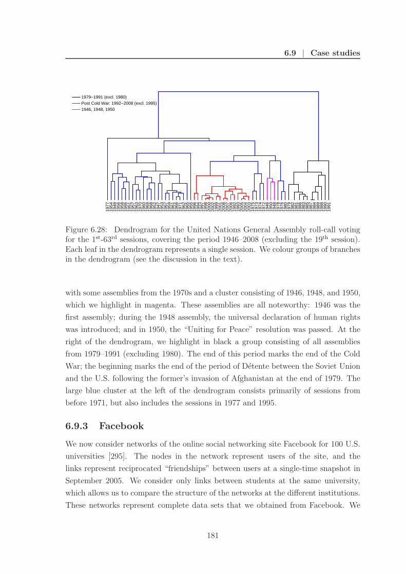
6.9 | Case studies
1977
1954
1949
1956
1958
1995
1951
1957
1963
1970
1960
1969
1968
1952
1947
1953
1967
1959
1961
1966
1971
1962
1965
1955
1996
1994
1997
1998
2000
2002
1999
2001
2008
2007
2006
1992
1993
2005
2004
2003
1975
1973
1974
1972
1946
1950
1948
1978
1976
1980
1979
1982
1981
1986
1983
1985
1987
1984
1989
1988
1990
1991
1979−1991 (excl. 1980)Post Cold War: 1992−2008 (excl. 1995)1946, 1948, 1950
Figure 6.28: Dendrogram for the United Nations General Assembly roll-call votingfor the 1st-63rd sessions, covering the period 1946–2008 (excluding the 19th session).Each leaf in the dendrogram represents a single session. We colour groups of branchesin the dendrogram (see the discussion in the text).
with some assemblies from the 1970s and a cluster consisting of 1946, 1948, and 1950,
which we highlight in magenta. These assemblies are all noteworthy: 1946 was the
first assembly; during the 1948 assembly, the universal declaration of human rights
was introduced; and in 1950, the “Uniting for Peace” resolution was passed. At the
right of the dendrogram, we highlight in black a group consisting of all assemblies
from 1979–1991 (excluding 1980). The end of this period marks the end of the Cold
War; the beginning marks the end of the period of Detente between the Soviet Union
and the U.S. following the former’s invasion of Afghanistan at the end of 1979. The
large blue cluster at the left of the dendrogram consists primarily of sessions from
before 1971, but also includes the sessions in 1977 and 1995.
6.9.3 Facebook
We now consider networks of the online social networking site Facebook for 100 U.S.
universities [295]. The nodes in the network represent users of the site, and the
links represent reciprocated “friendships” between users at a single-time snapshot in
September 2005. We consider only links between students at the same university,
which allows us to compare the structure of the networks at the different institutions.
These networks represent complete data sets that we obtained from Facebook. We
181
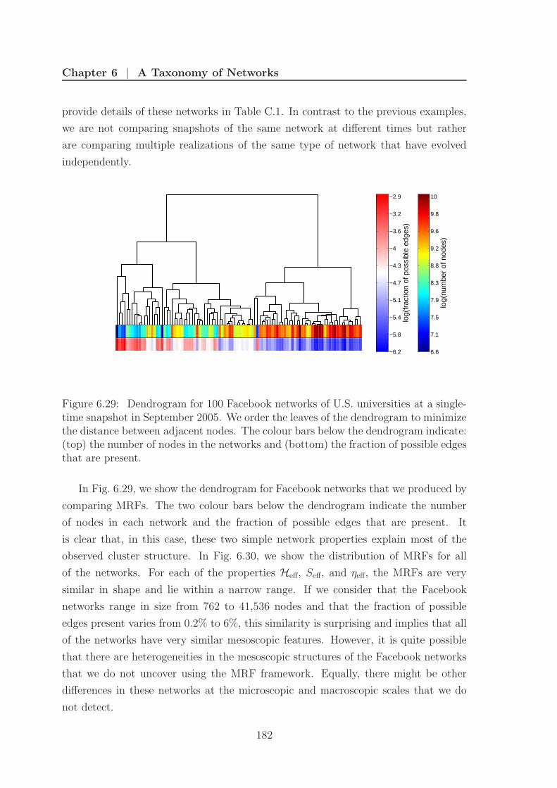
Chapter 6 | A Taxonomy of Networks
provide details of these networks in Table C.1. In contrast to the previous examples,
we are not comparing snapshots of the same network at different times but rather
are comparing multiple realizations of the same type of network that have evolved
independently.
log(
num
ber
of n
odes
)
6.6
7.1
7.5
7.9
8.3
8.8
9.2
9.6
9.8
10
log(
frac
tion
of p
ossi
ble
edge
s)
−6.2
−5.8
−5.4
−5.1
−4.7
−4.3
−4
−3.6
−3.2
−2.9
Figure 6.29: Dendrogram for 100 Facebook networks of U.S. universities at a single-time snapshot in September 2005. We order the leaves of the dendrogram to minimizethe distance between adjacent nodes. The colour bars below the dendrogram indicate:(top) the number of nodes in the networks and (bottom) the fraction of possible edgesthat are present.
In Fig. 6.29, we show the dendrogram for Facebook networks that we produced by
comparing MRFs. The two colour bars below the dendrogram indicate the number
of nodes in each network and the fraction of possible edges that are present. It
is clear that, in this case, these two simple network properties explain most of the
observed cluster structure. In Fig. 6.30, we show the distribution of MRFs for all
of the networks. For each of the properties Heff, Seff, and ηeff, the MRFs are very
similar in shape and lie within a narrow range. If we consider that the Facebook
networks range in size from 762 to 41,536 nodes and that the fraction of possible
edges present varies from 0.2% to 6%, this similarity is surprising and implies that all
of the networks have very similar mesoscopic features. However, it is quite possible
that there are heterogeneities in the mesoscopic structures of the Facebook networks
that we do not uncover using the MRF framework. Equally, there might be other
differences in these networks at the microscopic and macroscopic scales that we do
not detect.
182
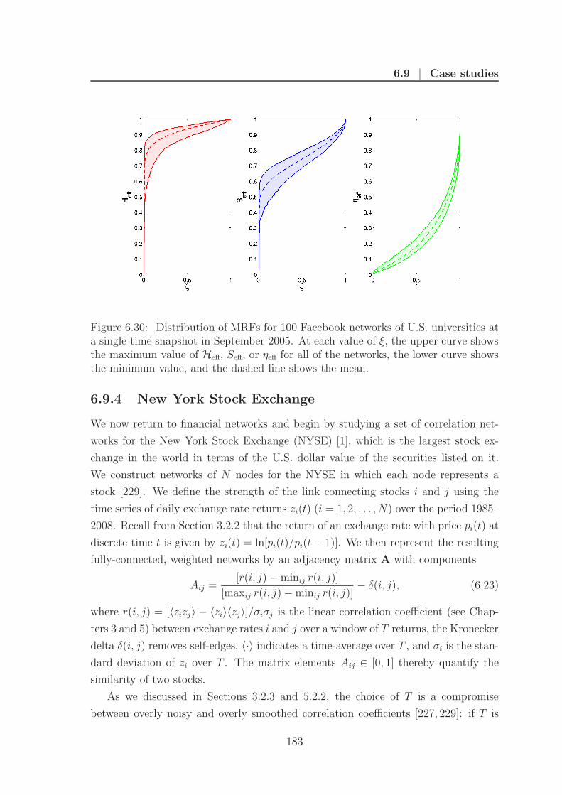
6.9 | Case studies
Figure 6.30: Distribution of MRFs for 100 Facebook networks of U.S. universities ata single-time snapshot in September 2005. At each value of ξ, the upper curve showsthe maximum value of Heff, Seff, or ηeff for all of the networks, the lower curve showsthe minimum value, and the dashed line shows the mean.
6.9.4 New York Stock Exchange
We now return to financial networks and begin by studying a set of correlation net-
works for the New York Stock Exchange (NYSE) [1], which is the largest stock ex-
change in the world in terms of the U.S. dollar value of the securities listed on it.
We construct networks of N nodes for the NYSE in which each node represents a
stock [229]. We define the strength of the link connecting stocks i and j using the
time series of daily exchange rate returns zi(t) (i = 1, 2, . . . , N) over the period 1985–
2008. Recall from Section 3.2.2 that the return of an exchange rate with price pi(t) at
discrete time t is given by zi(t) = ln[pi(t)/pi(t − 1)]. We then represent the resulting
fully-connected, weighted networks by an adjacency matrix A with components
Aij =[r(i, j) − minij r(i, j)]
[maxij r(i, j) − minij r(i, j)]− δ(i, j), (6.23)
where r(i, j) = [〈zizj〉 − 〈zi〉〈zj〉]/σiσj is the linear correlation coefficient (see Chap-
ters 3 and 5) between exchange rates i and j over a window of T returns, the Kronecker
delta δ(i, j) removes self-edges, 〈·〉 indicates a time-average over T , and σi is the stan-
dard deviation of zi over T . The matrix elements Aij ∈ [0, 1] thereby quantify the
similarity of two stocks.
As we discussed in Sections 3.2.3 and 5.2.2, the choice of T is a compromise
between overly noisy and overly smoothed correlation coefficients [227, 229]: if T is
183
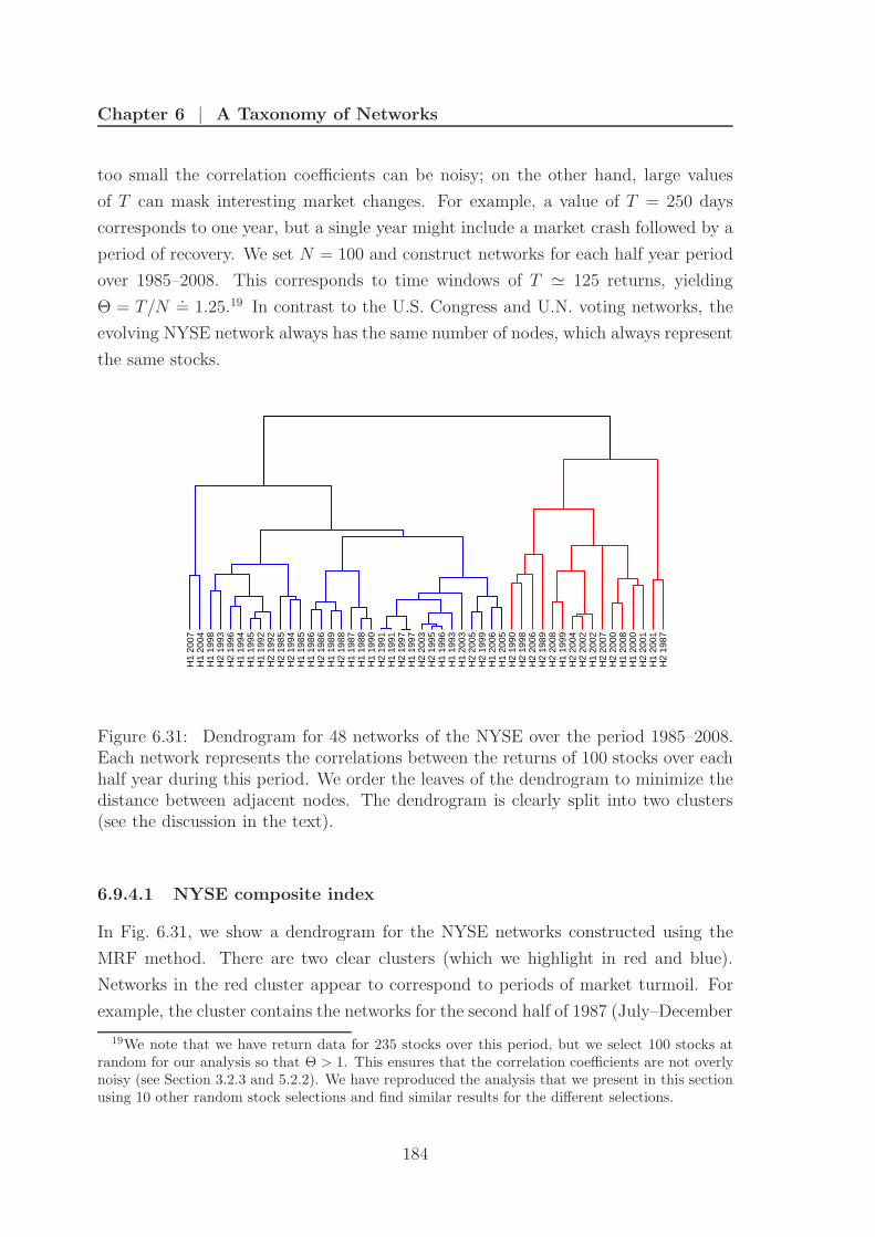
Chapter 6 | A Taxonomy of Networks
too small the correlation coefficients can be noisy; on the other hand, large values
of T can mask interesting market changes. For example, a value of T = 250 days
corresponds to one year, but a single year might include a market crash followed by a
period of recovery. We set N = 100 and construct networks for each half year period
over 1985–2008. This corresponds to time windows of T ≃ 125 returns, yielding
Θ = T/N.= 1.25.19 In contrast to the U.S. Congress and U.N. voting networks, the
evolving NYSE network always has the same number of nodes, which always represent
the same stocks.
H1
2007
H1
2004
H1
1998
H2
1993
H2
1996
H1
1994
H1
1995
H1
1992
H2
1992
H2
1985
H2
1994
H1
1985
H1
1986
H2
1986
H1
1989
H2
1988
H1
1987
H1
1988
H1
1990
H2
1991
H1
1991
H2
1997
H1
1997
H2
2003
H2
1995
H1
1996
H1
1993
H1
2003
H2
2005
H2
1999
H1
2006
H1
2005
H2
1990
H2
1998
H2
2006
H2
1989
H2
2008
H1
1999
H2
2004
H2
2002
H1
2002
H2
2007
H2
2000
H1
2008
H1
2000
H2
2001
H1
2001
H2
1987
Figure 6.31: Dendrogram for 48 networks of the NYSE over the period 1985–2008.Each network represents the correlations between the returns of 100 stocks over eachhalf year during this period. We order the leaves of the dendrogram to minimize thedistance between adjacent nodes. The dendrogram is clearly split into two clusters(see the discussion in the text).
6.9.4.1 NYSE composite index
In Fig. 6.31, we show a dendrogram for the NYSE networks constructed using the
MRF method. There are two clear clusters (which we highlight in red and blue).
Networks in the red cluster appear to correspond to periods of market turmoil. For
example, the cluster contains the networks for the second half of 1987 (July–December
19We note that we have return data for 235 stocks over this period, but we select 100 stocks atrandom for our analysis so that Θ > 1. This ensures that the correlation coefficients are not overlynoisy (see Section 3.2.3 and 5.2.2). We have reproduced the analysis that we present in this sectionusing 10 other random stock selections and find similar results for the different selections.
184

6.9 | Case studies
1987), which includes the Black Monday stock market crash of October 1987; all of
2000–2002, following the bursting of the dot-com bubble; and the second half of 2007
and all of 2008, which includes the recent credit and liquidity crisis.
We provide support for the hypothesis that the constituents of the red cluster
are networks for periods of market turmoil by considering the NYSE composite index
(NYSECI). The NYSECI measures the performance of all common stocks listed on the
NYSE by calculating the changes in their aggregate market value adjusted to eliminate
the effects of capitalization changes, new listings, and delistings. In Fig. 6.32, we
show the NYSECI as a function of time over the period 1985–2008 and highlight the
time periods that correspond to networks in the red cluster in the dendrogram in
Fig. 6.31. In Fig. 6.33, we show the volatility of the NYSECI over each half year
period. Volatility is usually high during periods of market turmoil. If we let χ(t)
represent the value of the index at time t, we can define a log-return zχ for the index
as zχ(t) = ln[χ(t)/χ(t − 1)]. We then define the volatility νχ of the NYSECI over a
window of T returns as [73]
νχ =1
T
T∑
t=1
| zχ(t) | . (6.24)
Figure 6.33 demonstrates that the networks assigned to the red cluster in Fig. 6.31
correspond (with one or two exceptions) to the periods of highest volatility. As we
noted above, the time window for a single network might include periods of both high
and low volatility, so it is unsurprising that the networks assigned to the red cluster
do not correspond exactly to the half year periods with the highest volatilities. This
remains true for all choices of T .
Although we study the same stocks over the full period 1985–2008, it is worth not-
ing that many of the companies might have changed significantly during these years.
For example, some of the companies might have expanded through acquisitions, while
others might have grown organically (i.e., through increased output, sales, or both).
Both of these processes could have altered the industries in which these companies
operate and led to significant changes in the nature of the stocks that we investigate.
The fact that we uncover a cluster corresponding to periods of market turmoil (and
do not simply uncover clusters corresponding to similar time periods) despite such
non-stationarities in the data is a testament to the effectiveness of the MRF clustering
framework.
185
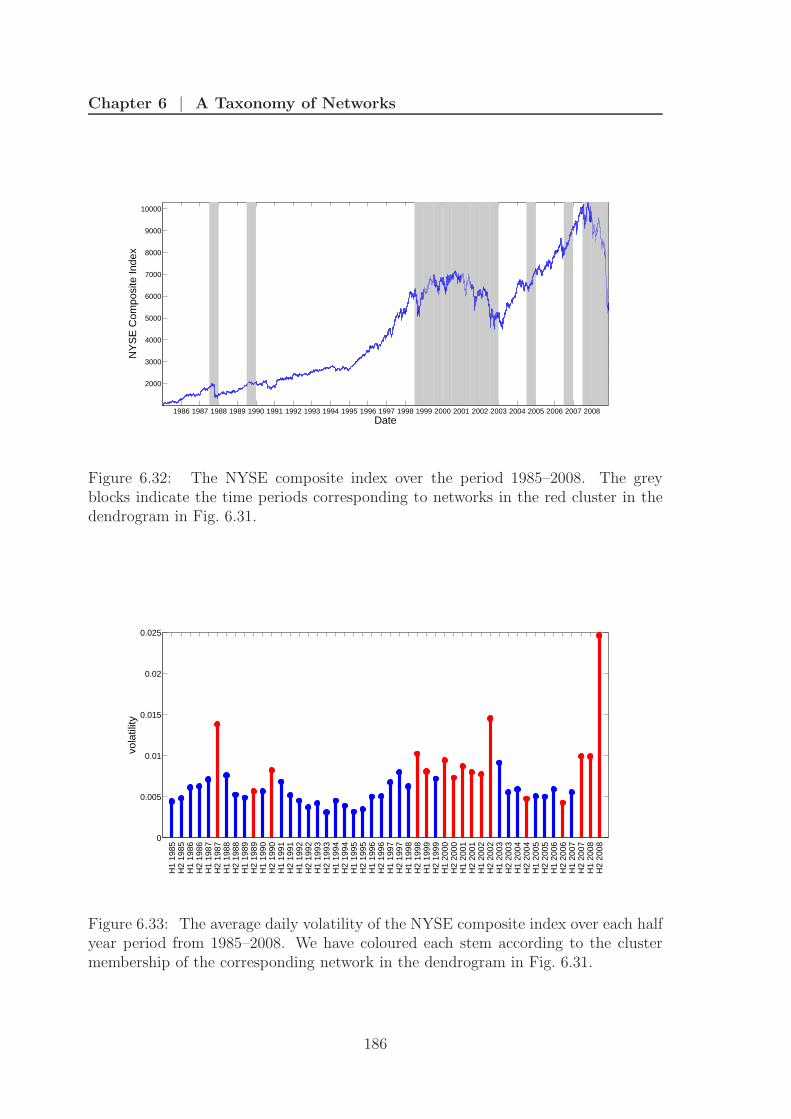
Chapter 6 | A Taxonomy of Networks
1986 1987 1988 1989 1990 1991 1992 1993 1994 1995 1996 1997 1998 1999 2000 2001 2002 2003 2004 2005 2006 2007 2008
2000
3000
4000
5000
6000
7000
8000
9000
10000
Date
NY
SE
Com
posi
te In
dex
Figure 6.32: The NYSE composite index over the period 1985–2008. The greyblocks indicate the time periods corresponding to networks in the red cluster in thedendrogram in Fig. 6.31.
0
0.005
0.01
0.015
0.02
0.025
H1
1985
H2
1985
H1
1986
H2
1986
H1
1987
H2
1987
H1
1988
H2
1988
H1
1989
H2
1989
H1
1990
H2
1990
H1
1991
H2
1991
H1
1992
H2
1992
H1
1993
H2
1993
H1
1994
H2
1994
H1
1995
H2
1995
H1
1996
H2
1996
H1
1997
H2
1997
H1
1998
H2
1998
H1
1999
H2
1999
H1
2000
H2
2000
H1
2001
H2
2001
H1
2002
H2
2002
H1
2003
H2
2003
H1
2004
H2
2004
H1
2005
H2
2005
H1
2006
H2
2006
H1
2007
H2
2007
H1
2008
H2
2008
vola
tility
Figure 6.33: The average daily volatility of the NYSE composite index over each halfyear period from 1985–2008. We have coloured each stem according to the clustermembership of the corresponding network in the dendrogram in Fig. 6.31.
186

6.9 | Case studies
6.9.5 Foreign exchange market
Our final example is a set of foreign exchange market networks. We use the data
described in Chapter 5 and define each network using Eq. 5 from Chapter 5. Each
network represents the correlations between the returns of 110 exchange rates over
each year during the period 1992–2008.20
In Fig. 6.34, we show the dendrogram of annual FX networks, which is clearly
split into two clusters. We highlight in green a sub-cluster within one of these clusters
for which the networks are particularly closely related. The years within this green
cluster are all years during which there was a major financial crisis: the Mexican
tequila crisis in 1994; the Asian crisis in 1997; the beginning of the Argentine crisis
and the devaluation of the Brazilian real in 1999; and the credit and liquidity crisis in
2007/2008. As a result, one could argue that this cluster represents years of financial
crisis. However, there are years during which there were major crises that are not
included in this cluster. For example, the withdrawl of the UK pound from the
European exchange rate mechanism in 1992 and the Russian rouble crisis in 1998.
There therefore seems to be an additional reason for the grouping of the networks in
the green cluster beyond the fact that they are all crisis years.
To further explain the clusters in the dendrogram, we consider the carry trade
return index Υ described in Section 5.8.3. We let Υ(t) represent the value of the
index at time t and define a log-return zΥ for the index as zΥ(t) = ln[Υ(t)/Υ(t− 1)].
We then define the volatility νΥ of the carry trade return index over a window of T
returns as
νΥ =1
T
T∑
t=1
| zΥ(t) | . (6.25)
In Fig. 6.34, we add a coloured bar under each leaf indicating the volatility νΥ of
the carry return index each year. For all of the years in the rightmost cluster (which
we highlight in red), the volatility of carry returns was low. Although other clusters
contain years during which the carry trade return volatility was low, the fact that all
years in the red cluster all have low volatility suggests that the carry trade explains
some of the observed structure in the dendrogram. Given the prevalence and impor-
tance of the carry trade in the FX market, this observation is perhaps unsurprising.
20We exclude 2003 and 2004 because we do not have data for these years.
187

Chapter 6 | A Taxonomy of Networks
2006
1992
1993
1996
1995
2007
2008
1999
1994
1997
2005
1998
2002
2000
2001
log(
ν ϒ)
−5.9
−5.8
−5.7
−5.6
−5.5
−5.4
−5.2
−5.1
−5
−4.9
Figure 6.34: Dendrogram for 15 foreign exchange market networks over the period1992–2008. Each network represents the correlations between the returns of 110 ex-change rates over each year during this period. We order the leaves of the dendrogramto minimize the distance between adjacent nodes. The dendrogram is split into twoclusters. We highlight one of these clusters in red and we highlight in green a sub-cluster within one of these clusters for which the networks are particularly closelyrelated. The colour bar under the dendrogram shows the volatility in the carry tradereturn index νΥ.
188

6.10 | Summary
6.9.6 Case studies summary
In this section, we have considered four case studies to demonstrate that the MRF
clustering scheme is able to produce meaningful taxonomies for a diverse range of
networks. In these examples, we can explain many of the observed clusters by prop-
erties that are unique to each type of network, but the MRF method can be applied
successfully in all of these cases. The wide range of areas for which the MRF cluster-
ing is successful thereby provides supporting evidence that the clusters that we see
in the aggregate taxonomy are meaningful.
6.10 Summary
We have developed a framework based on MRFs for comparing and clustering net-
works using their mesoscopic structures. We used this framework to create a taxon-
omy of networks and to identify groups of closely related networks and anomalous
networks that were not grouped with members of their class. In addition to clustering
networks of different types, we also created taxonomies for sub-sets of networks that
represent multiple realizations of the same type of system (Facebook networks) and
temporal snapshots of time-dependent systems (Congressional roll-call voting, U.N.
resolution, NYSE, and FX networks). For each example of time-ordered sequences of
networks, we identified periods during which there were significant changes in meso-
scopic structure.
189

Chapter 7
Conclusions
We began this thesis by investigating triangular arbitrage in the spot foreign exchange
market in Chapter 2. The aim of Chapter 2 was twofold: first, to answer a question of
interest to market practitioners, namely whether triangular arbitrage opportunities
exist; second, to demonstrate that when investigating financial markets it is essential
to ensure that one is using data that is appropriate to the question being posed. Using
executable price data, we demonstrated that although triangular arbitrage opportu-
nities appear to exist in the foreign exchange market, most of these opportunities
are very short in duration and represent very small profit opportunities. We further
showed that, when one also considers the strong competition for each arbitrage and
trading and technology costs, a trader would need to beat other market participants
to an unfeasibly large proportion of arbitrage opportunities for triangular arbitrage
to remain profitable in the long-term. These results provide a limited verification of
foreign exchange market efficiency.
In Chapter 3, we extended our analysis of financial markets beyond the foreign
exchange market and considered a variety of other markets, including equities, bonds,
and commodities. We investigated these markets by constructing correlation matri-
ces for the time series of asset returns and analyzed the temporal changes in the
structure of these correlations. The number of correlations scales as the square of the
number of assets N , so some simplification was necessary to identify the key relation-
ships. We coarse-grained the correlation matrix using principal component analysis
to identify the important relationships and analyzed the evolution of the system by
considering the changes in the principal components. We found that the percentage
of the variance in market returns accounted for by the first principal component rose
steadily between 1999 and 2008 but then increased sharply following the 2008 collapse
of Lehman Brothers. We further found that during this period the number of signifi-
cant components decreased and the number of assets making significant contributions
191

Chapter 7 | Conclusions
to the first principal component increased. To gain some insights into the relation-
ships between the different assets, we considered the correlations between the asset
return time series and the principal components. Initially, the first few components
appeared to represent different asset classes. For example, the first component corre-
sponded to bonds, the second to equities, and the third to currencies. However, later
in the studied period these relationships began to break down. In fact, by January
2010 nearly all of the studied assets were significantly correlated with the first prin-
cipal component and relatively few assets were significantly correlated with the other
components. This suggests that there are more common features across markets in
2010 than there were in 1999.
In Chapter 4, we described some of the most widely used methods for detecting
communities in networks and presented a relatively comprehensive review of the liter-
ature on communities in dynamic networks. In Chapter 5, we presented an alternative
method for investigating evolving correlation matrices in which we represented the
correlation matrices as time-dependent networks and investigated the dynamics of
network communities. We proposed a method for tracking communities through time
from the perspective of individual nodes, which removes the undesirable requirement
of determining which community at each time step represents the descendant of a
community at the previous time step. We applied this technique to foreign exchange
market networks in which each node represents an exchange rate and each edge rep-
resents a time-dependent correlation between the rates. Our analysis successfully
uncovered significant structural changes that occurred in the foreign exchange mar-
ket, including ones that resulted from major market events, and we demonstrated that
community reorganizations at specific time steps can provide insights into changes in
trading behaviour. We also considered the evolving relationship between individual
nodes and their community and demonstrated that an exchanges rate’s functional
role is related to its position within its community, with exchange rates that are im-
portant for information transfer located on the edges of communities and exchange
rate that have a strong influence on other rates within that community located at the
centre of their community.
Finally, in Chapter 6, we introduced mesoscopic response functions to characterize
the community structures of networks. Importantly, the response functions are nor-
malized so that it is possible to compare networks of significantly different sizes and
connectivities. We used the response functions to compare and cluster networks and
created a taxonomy of networks from a wide variety of different fields. The taxon-
omy contained many clusters that included networks from the same family, but there
192

7.1 | Outlook
were also examples of networks not clustered with networks that were nominally of
the same type. In this way, the framework that we propose can be used to identify
anomalous members of a family of networks.
As well as creating a taxonomy of networks from different fields, we also created
taxonomies for subsets of networks that represent multiple realizations of the same
type of system and temporal snapshots of time-dependent systems. For example, we
created a taxonomy for a time-sequence of New York Stock Exchange networks which
was split into two clusters based on the volatility of the market over the corresponding
period. We also created taxonomies of roll-call voting in the U.S. Senate and House
of Representatives in which the cluster membership of the different Congressional
sessions was determined by the levels of party polarization. Although we can explain
many of the observed clusters by properties that are unique to each type of network
in the intra-family taxonomies, the mesoscopic response function framework provides
insights in all of the different case studies.
7.1 Outlook
For much of this thesis we focused on financial networks and network communities, so
we conclude with some comments on the current state of both fields and we discuss
potential directions for future research.
In Chapter 5, we studied communites in foreign exchange market networks, but
the techniques that we presented are general and can be applied to networks for other
asset classes. In fact, the Potts methods has already been used to study communities
in a network of equities [148]. However, in Ref. [148] Heimo et al. only examine com-
munities in a static network of stocks traded on the New York Stock Exchange and do
not study longitudinal networks. A potential area for future research is, therefore, to
investigate community dynamics in evolving networks of equities. In equity markets,
stocks are usually assigned to industry sectors based on the business activities of the
companies; these sectors provide a useful tool for sorting and comparing different
companies. For example, it is often insightful to compare the performance of stocks
within the same sector to find out if any are under-performing (or over-performing)
compared with the rest of the sector. An interesting avenue for future research would
be to compare the communities identified using the Potts method with the sector
classifications to see if they line up well or if there are periods during which there are
significant differences in the classifications.
193

Chapter 7 | Conclusions
One issue with using the Potts method to investigate communities in longitudinal
equity networks is that in previous work [148] plateaus have not been observed in plots
of the number of communities as a function of the resolution parameter (see Section
5.4).1 The absence of a plateau means that it is not possible to use the approach
described in Section 5.4 to select the resolution at which to investigate community
dynamic, so other methods will need to be developed.
We have focused on financial networks constructed from correlation matrices of
asset price time series, but other types of financial networks have also been studied
(see Ref. [11] for an overview of the applications of networks in finance). For example,
networks have been used to analyze the trade relationships between nations, e.g.,
[266,275], and the credit relationships between financial institutions, e.g., [31,52,116].
The latter subject has received particular attention in the last few years as a result
of the 2007–2008 credit and liquidity crisis. During the credit crisis, difficulties in
the U.S. subprime mortgage market soon spread to debt markets all over the world,
and eventually resulted in credit drying up as banks became unwilling to lend as
freely [11]. The market turmoil clearly demonstrated the interconnectedness of the
global financial system and how this connectivity can lead to outcomes that are
difficult to forecast. As a consequence, the study of credit networks is currently one
of the most active areas of research in financial networks and is an important direction
for future research.
In the standard representation of a credit network, the nodes represent financial
institutions and the edges represent credit relationships. A key concern in the study
of such networks is how the insolvency of particular institutions affects the network;
in particular, whether the failure of individual banks is “contagious” and leads to
a systemic crisis in which a large fraction of the firms in the system fail at the
same time [31]. One of the most important questions for understanding this risk is
how connectivity affects network robustness [31, 116, 202], which is closely related to
questions asked in ecology [202]. In Ref. [12], Allen and Gale studied how the banking
system responds to contagion when banks are connected under different network
structures. They found that networks with higher connectivities are more resilient
and have a lower likelihood of widespread default because the losses sustained by one
bank are transferred to more banks through interbank agreements. However, Gai and
Kapadia [116] reached a different conclusion. They agreed that greater connectivity
1Recall that community partitions that are robust across a range of resolutions are significantbecause the communities do not break up despite an increasing incentive to do so. Communitiesthat persist over a large range of resolutions thus potentially represent important substructures.
194

7.1 | Outlook
reduces the likelihood of contagion, but it also means that if a problem does occur
the shocks could be on a significantly larger scale. Battiston et al. [31] make similar
observations. They found that although increased connectivity can reduce the risk
of the collapse of an individual node through risk sharing, it can also result in crises
being more severe and more frequent.
The lack of a consensus on the most robust structure for banking networks means
that this is a particularly crucial area for future research. One of the major questions
in this context is whether networks organized into communities have lower systemic
risk [31]. Ecologists have suggested that decoupling a system into relatively discrete
components can promote robustness [202]; however, this is not a simple question
because some partitions of financial networks into communities could potentially pre-
clude stabilizing effects such as mechanisms for maintaining liquidity [161]. Some
steps have been taken to investigate communities in credit networks, e.g., [195], but
there are still many unanswered questions. An interesting direction for future re-
search would be to apply the methods that we presented in Chapter 5 to directed
networks representing the evolving credit relationships between financial institutions
during the 2007–2008 credit crisis.2
In the wider study of community structure in networks, significant technical
advances have been made in recent years, and it remains a thriving area of re-
search [105,244]. Typically, the first stage of community analysis is the identification
of the communities; indeed, this is the subject of many of the papers in the literature
and a wealth of different techniques have been proposed for the algorithmic detec-
tion of communities. However, researchers have not yet agreed on which methods
are most appropriate or reliable or when particular methods should be adopted or
avoided. The problem of assessing the reliability of the output of different algorithms
is exacerbated by the fact that there is no rigorous definition of a community. The
most rigorous approach that is currently available is to identify communities using
different detection algorithms and only to consider structures that are similar across
multiple methods as meaningful [244, 289]. In this way, one can be more sure that
the identified structures are genuine features of the data and not simply byproducts
of the detection algorithm.
Even with the focus on developing community detection algorithms, very little
attention has been paid to validating the output of the detection algorithms and
trying to understand what the communities mean, what they actually look like or
2Although we focused on undirected networks in Chapters 5 and 6, the techniques that weintroduced in these chapters can easily be extended to directed networks.
195

Chapter 7 | Conclusions
how they can be used [105, 181, 222, 244]. Some steps have now been taken towards
answering some of these questions. For example, in Ref. [295] the composition of
communities is related to the demographic characteristics of nodes and in Ref. [181]
the structure and properties of communities in a range of different networks, including
biological, social, and communication networks, have been studied and compared. In
this thesis, we have also contributed to this endeavour. For example, in Chapter 5
we used the composition of different communities to uncover changes taking place
in trading behaviour within the foreign exchange market and in Chapter 6 we used
communities to create a taxonomy of networks. However, much still remains to be
done in this direction and this is arguably the most pressing area of research if we
are to gain real insights from studies of network community structures.
There are similar open questions in the study of dynamic communities (see Sec-
tion 4.6.13). With a few exceptions, the studies of dynamic communities present a
method for detecting communities, check that the identified communities make sense,
and then stop. There are very few studies that investigate the mechanisms that drive
the community evolution or try to answer some of the fundamental questions relating
to dynamic communities, such as what community properties result in stable commu-
nities and what features of a community determine whether an individual will join (or
leave) that community. In Chapter 5, we attempted to answer some of these questions
for the foreign exchange market. For example, we demonstrated that nodes that have
strong connections with their communities tend to have more stable community rela-
tionships than nodes with weak connections. The limited progress in the study of the
properties of dynamic communities is perhaps unsurprising given the relative infancy
of the field; hence, it represents an important direction for future research [318].
Another direction for future research is the development of algorithms that can
identify overlapping communities. Most existing community detection algorithms
generate partitions in which each node is assigned to exactly one community. How-
ever, this does not reflect the structure of many real-world systems. For example,
in social networks people can belong to communities of friends, communities of work
colleagues, and family communities. Some methods have been developed that can
identify overlapping communities, e.g., [32, 234]. Perhaps the most widely used is
the clique percolation method [234] that we described in Section 4.3.1; however, as
we highlighted, this approach has limitations, so alternative techniques need to be
developed.
The methods in Refs. [32,234] allow nodes to belong to more than one community,
but do not give any indication of the community with which a node is most closely
196

7.1 | Outlook
associated. Therefore, another possibility is algorithms that do not assign nodes to
one or to multiple communities, but instead assign each node a weight indicating the
strength of its attachment to each community [215, 317]. By normalizing the sum
of each node’s community affiliation to unity, this measure can be interpreted as the
probability that a node belongs to a particular community. Along similar lines, models
have been proposed in the dynamic communities literature that give a probability that
each node belongs to each community at different time steps, e.g., [186].
All of the community detection methods that we have discussed so far have focused
on partitioning the entire network into communities, i.e., all of the methods associate
every node in the network with at least one community. However, many real-world
network contain nodes that do not fit into any community particularly well. With this
in mind, a recent paper [318] has proposed a method that broadens the community
detection framework by allowing a network to contain not only communities but also
background nodes that are not associated with any community.
Finally, the typical motivation for studies of communities is that the community
structure of a network has some bearing on its function. Most studies then use struc-
tural communities as proxies for functional communities. However, the functional
and structural properties of a system sometimes do not map onto each other, so it is
likely that structural communities do not always correspond to functional communi-
ties [271]. For example, studies of neural networks have shown that it is fairly common
for central pattern generators3 to change their functional organization, depending on
the pattern that they are generating, while maintaining a constant anatomical struc-
ture [268]. Consequently, an important avenue for future research is the development
of techniques that detect communities using both functional and structural informa-
tion.
This represents just a small sample of open questions relating to networks com-
munities, which is itself just a sub-area of the field of networks, and many other open
questions exist in the wider field. It will be interesting to see how the analysis of
communities and the field of networks matures over the next few years and whether
it can maintain the current rate of development.
3Central pattern generators are the neuronal circuits that give rise to repetitive or oscillatorypatterns of muscle activity that produce rhythmic movements, such as locomotion, breathing, andchewing [54].
197


Appendix A
Details of Financial Assets
Table A.1: Details of all of the financial assets studied in Chapter 3. The data that weuse in this chapter was downloaded from Bloomberg. See http://www.bloomberg.
com/ for more information on the different financial instruments.
Ticker Sector Description
AEX Equities AEX Index (Netherlands)AS30 Equities Australian All Ordinaries IndexASE Equities Athens Stock Exchange General IndexATX Equities Austrian Traded IndexBEL20 Equities BEL 20 Index (Belgium)BVLX Equities PSI General Index (Portugal)CAC Equities CAC 40 Index (France)DAX Equities DAX Index (Germany)FTSEMIB Equities FTSE MIB Index (Italy)HEX Equities Helsinki Stock Exchange General IndexHSI Equities Hang Seng Index (Hong Kong)IBEX Equities IBEX 35 Index (Spain)INDU Equities Dow Jones Industrial Average Index (U.S.)ISEQ Equities Irish Overall IndexKFX Equities OMX Copenhagen 20 IndexNDX Equities NASDAQ 100 Index (U.S.)NKY Equities Nikkei 225 Index (Japan)NZSE Equities New Zealand All Ordinaries IndexOBX Equities OBX Stock Index (Norway)OMX Equities OMX Stockholm 30 IndexRTY Equities Russell 2000 Index (U.S.)SMI Equities Swiss Market IndexSPTSX Equities S&P/Toronto Stock Exchange IndexSPX Equities Standard and Poor’s 500 (U.S.)UKX Equities FTSE 100 Index (U.K.)GDDUEMEA Equities Emerging markets: Europe, Middle East, AfricaGDUEEGFA Equities Emerging markets: AsiaGDUEEGFL Equities Emerging markets: Latin America
continued on next page
199

Appendix A
Ticker Sector Description
ATGATR Government bonds Austrian government bondsAUGATR Government bonds Australian government bondsBEGATR Government bonds Belgian government bondsCAGATR Government bonds Canadian government bondsDEGATR Government bonds Danish government bondsFIGATR Government bonds Finnish government bondsFRGATR Government bonds French government bondsGRGATR Government bonds German government bondsIEGATR Government bonds Irish government bondsITGATR Government bonds Italian government bondsJNGATR Government bonds Japanese government bondsNEGATR Government bonds Netherlands government bondsNOGATR Government bonds Norwegian government bondsNZGATR Government bonds New Zealand government bondsPTGATR Government bonds Portuguese government bondsSPGATR Government bonds Spanish government bondsSWGATR Government bonds Swedish government bondsSZGATR Government bonds Swiss government bondsUKGATR Government bonds U.K. government bondsUSGATR Government bonds U.S. government bondsAUDUSD Currencies Australian dollarCADUSD Currencies Canadian dollarCHFUSD Currencies Swiss francCZKUSD Currencies Czech korunaEURUSD Currencies EuroGBPUSD Currencies Pounds sterlingIDRUSD Currencies Indonesian rupiahJPYUSD Currencies Japanese yenKRWUSD Currencies Korean wonMXNUSD Currencies Mexican pesoNOKUSD Currencies Norwegian kroneNZDUSD Currencies New Zealand dollarPHPUSD Currencies Philippines pesoSEKUSD Currencies Swedish kronaZARUSD Currencies South African randHG1 Metals CopperLA1 Metals AluminiumLL1 Metals LeadLN1 Metals NickelLT1 Metals TinXAG Metals SilverXAU Metals GoldXPD Metals PalladiumXPT Metals PlatinumCL1 Fuels Crude oil, WTI
continued on next page
200

Details of Financial Assets
Ticker Sector Description
CO1 Fuels Crude oil, brentHO1 Fuels Heating oilNG1 Fuels Natural gasBO1 Commodities Soybean oilC 1 Commodities CornCC1 Commodities CocoaCT1 Commodities CottonFC1 Commodities CoffeeJN1 Commodities Feeder cattleJO1 Commodities Orange juiceKC1 Commodities CoffeeLB1 Commodities LumberLC1 Commodities Live cattleLH1 Commodities Lean hogsO 1 Commodities OatsPB1 Commodities Frozen pork belliesQW1 Commodities SugarRR1 Commodities Rough riceS 1 Commodities SoybeanSM1 Commodities Soybean mealW 1 Commodities WheatMOODCAAA Corporate bonds Moody’s AAA corporate bondsMOODCAA Corporate bonds Moody’s AA corporate bondsMOODCA Corporate bonds Moody’s A corporate bondsMOODCBAA Corporate bonds Moody’s BAA corporate bonds
201


Appendix B
Robustness of FX Communities toAlternative Heuristics
In this section, we demonstrate that the results described in Chapter 5 are robust with
respect to the choice of computational heuristic used to minimize the Hamiltonian in
Eq. 4.3.
B.1 Comparison of partition energies
We begin by comparing the energy H (see Eq. 4.3) of the optimal partitions at
the studied resolution λ = 1.45. Figure B.1 shows the distribution of energies for
the different algorithms and demonstrates that the greedy algorithm and simulated
annealing find better partitions than the spectral algorithm. The spectral algorithm
begins by splitting the network into two components, choosing the split that minimizes
the energy, and then recursively partitions the smaller networks into two groups
until no decrease in energy can be obtained through partitioning. At each step,
the algorithm only finds the optimal partition of each community into two smaller
communities, even though a split into more communities might yield a lower energy.
Given this, it is unsurprising that the spectral algorithm identifies partitions further
from the optimum than the other heuristics. For the remainder of this section, we
will only compare the greedy and simulated annealing algorithms because of the lower
quality of the spectral partitions.
B.2 Temporal changes in communities
First, we compare the community partitions identified by the two heuristics for each
network. In Fig. B.2, we show the distribution of the variation of information be-
203
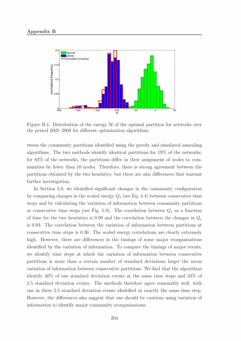
Appendix B
−250 −200 −150 −100 −50 0 500
0.05
0.1
0.15
0.2
H
norm
aliz
ed fr
eque
ncy
spectralgreedysimulated annealing
Figure B.1: Distribution of the energy H of the optimal partition for networks overthe period 2005–2008 for different optimization algorithms.
tween the community partitions identified using the greedy and simulated annealing
algorithms. The two methods identify identical partitions for 19% of the networks;
for 83% of the networks, the partitions differ in their assignment of nodes to com-
munities by fewer than 10 nodes. Therefore, there is strong agreement between the
partitions obtained by the two heuristics, but there are also differences that warrant
further investigation.
In Section 5.8, we identified significant changes in the community configuration
by comparing changes in the scaled energy Qs (see Eq. 4.4) between consecutive time
steps and by calculating the variation of information between community partitions
at consecutive time steps (see Fig. 5.9). The correlation between Qs as a function
of time for the two heuristics is 0.99 and the correlation between the changes in Qs
is 0.93. The correlation between the variation of information between partitions at
consecutive time steps is 0.36. The scaled energy correlations are clearly extremely
high. However, there are differences in the timings of some major reorganizations
identified by the variation of information. To compare the timings of major events,
we identify time steps at which the variation of information between consecutive
partitions is more than a certain number of standard deviations larger the mean
variation of information between consecutive partitions. We find that the algorithms
identify 40% of one standard deviation events at the same time steps and 33% of
2.5 standard deviation events. The methods therefore agree reasonably well, with
one in three 2.5 standard deviation events identified at exactly the same time step.
However, the differences also suggest that one should be cautious using variation of
information to identify major community reorganizations.
204

Robustness of FX Communities
0 0.05 0.1 0.15 0.2 0.25 0.30
0.05
0.1
0.15
0.2
0.25
V
norm
aliz
ed fr
eque
ncy
Figure B.2: The distribution of the variation of information between communitypartitions identified using the greedy algorithm and simulated annealing for networksover the period 2005–2008.
B.3 Example community comparison
One time step at which both heuristics identify a large community change is 15/08/07
which, as described in Section 5.8.3, was a day when there was a significant increase
in carry trade unwinding. It is worth considering the communities at this time step in
detail to help assess the similarity of the results for the two heuristics. In Fig. B.3(a),
we show the communities that we identified using a greedy algorithm [44] immediately
before and after 15/08/07; in Fig. B.3(b) we show communities that we identified
using simulated annealing [141] for the same time steps. Figure B.3(a) shows that,
leading up to 15/08/07, there was some unwinding of the carry trade, so the initial
configuration includes a community containing exchange rates of the form AUD/YYY,
NZD/YYY, and XXX/JPY (which all involve one of the key carry-trade currencies).
After 15/08/07, as the volume of carry trade unwinding increases, this community
incorporates other XXX/JPY rates as well as some XXX/CHF and XXX/USD rates.
Although, the communities in Fig. B.3(b) for the simulated annealing algorithm are
not identical to those in Fig. B.3(a), they are very similar. The main difference is that
for the simulated annealing algorithm, there are two carry trade communities before
15/08/07: one community of exchange rates of the form AUD/YYY, NZD/YYY
(which are all exchange rates that include a carry trade investment currency) and
another community containing exchange rates of the form XXX/CHF and XXX/JPY
(which are all exchange rates that include a carry trade funding currency). After
15/08/07, as carry trade unwinding increases, these two communities combine and
205

Appendix B
two other exchange rates also join the community. The resulting merged community
is very similar to the largest community identified at the same time step using the
greedy algorithm.
Figure B.3 therefore illustrates that there are only small differences in the com-
munity configurations that are identified by the two heuristics. In fact, as Fig. B.2
shows, the two algorithms agree in the assignment of all but about ten nodes approx-
imately 80% of the time. Importantly, Fig. B.3 highlights that, even when there are
differences in the exact community configurations, the communities that are identi-
fied by the two heuristics nonetheless indicate the same changes taking place in the
FX market.
Figure B.3: Comparison of the change in community structure in one half of theFX market network over the same period for different optimization heuristics. Weshow a schematic of the communities for the period following 15/08/07, when therewas significant unwinding of the carry trade during the 2007–2008 credit and liquiditycrisis. We identified communities using (a) a greedy algorithm [44] and (b) a simulatedannealing algorithm [141]. The node colours after the community reorganizationcorrespond to their community before the change. If the parent community of acommunity after the reorganization is obvious, we draw it using the same colour asits parent. The nodes drawn as triangles resided in the opposite half of the networkbefore the community reorganization.
206

Robustness of FX Communities
B.4 Node role comparison
As a further comparison, we investigate the effect of different heuristics on exchange
rate roles (see Section 5.9). In Fig. B.4, we compare quarterly role evolutions over the
period 2005–2008 for the same exchanges rate shown in Fig. 5.15. Although there are
slight differences in the positions of the exchange rates in the (κb, κy) plane for some
periods, we obtain the same aggregate conclusions. For example, for both heuristics,
AUD/JPY is most influential within its community (high κb) during Q3 and Q4 2007
and during Q1 and Q4 2008; however, it is less influential, but more important for
information transfer, during 2005 and 2006.
The positions in the (κb, κy) plane are similarly close for all of the other exchange
rates. We quantify the differences in the positions for the two heuristics by calculating
the mean and standard deviation of the change in position over all exchange rates
and over all time periods. That is, we average the change in position of every node
in the (κb, κy) plane over every quarter. The mean change in position in both the
κb and κy directions is less than 10−4; the standard deviations are 0.15 and 0.17,
respectively. However, because the changes in position are likely to cancel out (i.e.,
an increase in κb for one exchange rate is likely to be offset by a decrease in κb for
another exchange rate), it is more informative to calculate the mean and standard
deviation of the absolute changes in position in the κb and κy directions. In the κb
direction, the mean absolute change in position is 0.08, with a standard deviation
of 0.13; in the κy direction, the mean change is 0.09, with a standard deviation of
0.15. The mean differences in positions in the (κb, κy) are therefore very small for the
two heuristics and, as Fig. B.4 demonstrates, both algorithms uncover the same role
changes in the FX market for the different exchange rates.
Finally, we also checked the relationships shown in Fig. 5.8 between the community
centrality and community size, between the community alignment and betweenness
centrality, and between the community autocorrelation and projected community cen-
trality. Using simulated annealing, we find the same relationships that we uncovered
with the greedy algorithm.
The results of this section demonstrate that, although there are differences in the
communities identified using different optimization heuristics, the aggregate conclu-
sions are the same. We identify the same changes taking place in the FX market
whether we use the greedy algorithm or simulated annealing to minimize energy.
The fact that we obtain very similar results using different optimization techniques,
207
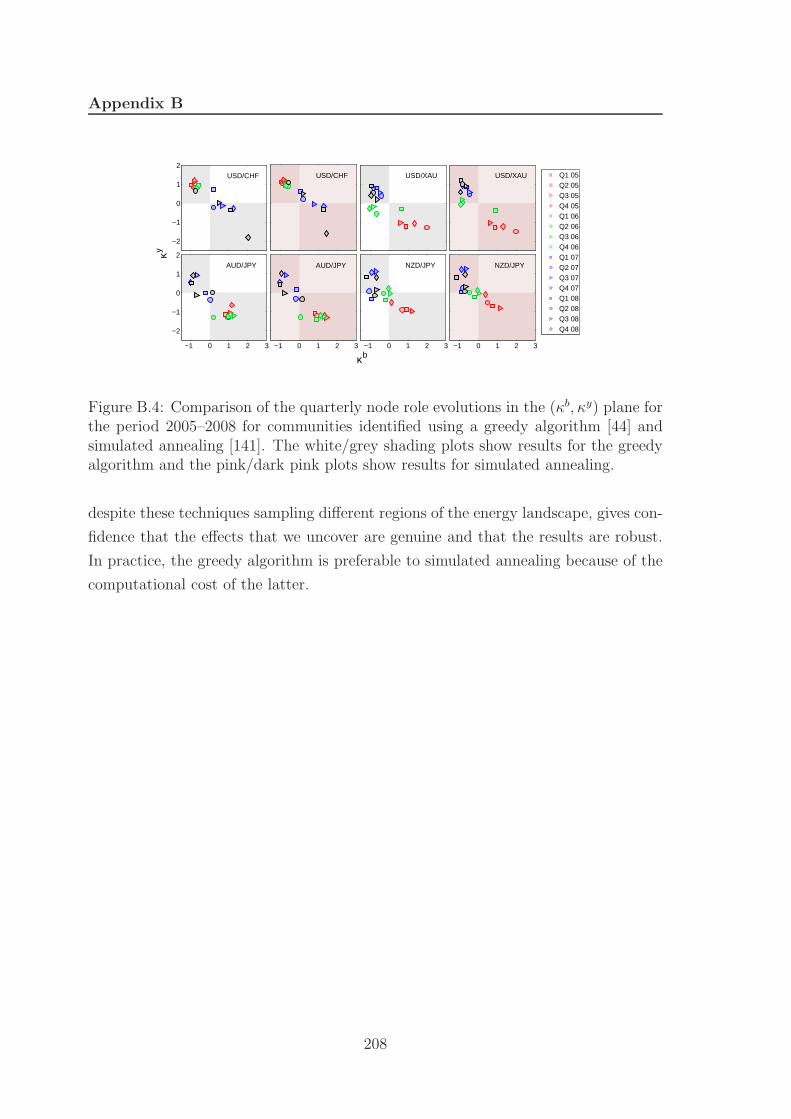
Appendix B
Q1 05Q2 05Q3 05Q4 05Q1 06Q2 06Q3 06Q4 06Q1 07Q2 07Q3 07Q4 07Q1 08Q2 08Q3 08Q4 08
NZD/JPY
κb
−1 0 1 2 3
AUD/JPY
−1 0 1 2 3
−2
−1
0
1
2
USD/XAUUSD/CHF
κy
−2
−1
0
1
2USD/CHF USD/XAU
AUD/JPY
−1 0 1 2 3
NZD/JPY
−1 0 1 2 3
Figure B.4: Comparison of the quarterly node role evolutions in the (κb, κy) plane forthe period 2005–2008 for communities identified using a greedy algorithm [44] andsimulated annealing [141]. The white/grey shading plots show results for the greedyalgorithm and the pink/dark pink plots show results for simulated annealing.
despite these techniques sampling different regions of the energy landscape, gives con-
fidence that the effects that we uncover are genuine and that the results are robust.
In practice, the greedy algorithm is preferable to simulated annealing because of the
computational cost of the latter.
208
Appendix C
Network Details
In Table C.1, we provide details of the networks studied in Chapter 6. We include
several synthetic network families and benchmark networks that were introduced
to test community detection algorithms. For many of these, we include multiple
realizations that we obtained using different parameter values. We briefly describe
these networks and explain the notation we use to label them in Table C.1.
Erdos-Renyi (ER): In an ER network of N nodes, each pair of nodes is connected
by an unweighted edge with probability p and not connected with probability
1 − p [86]. The degree of each node is distributed according to a binomial
distribution. We label the ER networks using the notation “ER: (N ,p)”.
Watts-Strogatz (WS): We consider the small-world network of Watts and Stro-
gatz [305] for a one-dimensional lattice of N nodes with periodic boundary
conditions. The network consists of a ring in which each node is connected with
an unweighted edge to all of its neighbours that are k or fewer lattice spacings
away. Each edge is then visited in turn and one end is rewired with probability
p to a different node selected uniformly at random, subject to the constraint
that there can be no self-edges or double-edges. We label each Watts-Strogatz
network as “WS: (N ,k,p)”.
Barabasi-Albert (BA): BA networks [26] are obtained using a network growth
mechanism in which nodes with degree m are added to the network and the
other end of each edge attaches to another node with a probability proportional
to the degree of that node. We label each BA network “BA: (N ,m)”.
Fractal: We generate fractal networks using the method described in Ref. [279]. We
begin by generating an isolated group of 2m fully-connected nodes, where m is
209

Appendix C
the size of the clusters. These groups correspond to the hierarchical level h = 0.
We then create a second identical group and we link the two groups with a link
density of E−h (h = 1), where the link density is the number of links out of all
possible links between the groups and E gives the connection density fall-off per
hierarchical level. We then duplicate this network and connect the two dupli-
cates at the level h = 2 with a link density E−2. We repeat this until we reach
the desired network size N = 2n, where n is the number of hierarchical lev-
els. At each step the connection density is decreased, resulting in progressively
sparser interconnectivity at higher hierarchical levels. The resulting network
exhibits self-similar properties. We label each network “Fractal: (n, m, E)”.
Random fully-connected: We produce random, fully connected networks of N
nodes by linking every node to every other node with an edge whose weight is
chosen uniformly at random on the unit interval. The networks have N(N−1)/2
edges. We label each network “Random fully-connected: (N)”.
Kumpula-Onnela-Saramaki-Kaski-Kertesz (KOSKK) model: We generate
weighted networks containing communities using the model described in [174].
We create links through two mechanisms: First, at each time step, each node
i selects a neighbour j with probability wij/si, where wij is the weight of of
the link connecting i and j and si =∑
j wij is the strength of i. If j has
other neighbours in addition to i, then one of them is selected with probability
wjk/(sj −wij). If i and k are not connected, then a new link of weight wik = w0
is created with probability pn. If the link already exists, its weight is increased
by an amount δ. In both cases, wij and wjk are also increased by δ. This pro-
cess is termed local attachment. Second, if a node has no links, with probability
pr, it creates a link of weight w0 to a randomly selected node, which is termed
global attachment. A node can be deleted with probability pd, in which case all
of its links are also removed and it is replaced by a new node, so that the total
number of nodes N remains constant. The mechanism begins with an empty
network, and links are added by running the local and global attachment mech-
anisms in parallel. We label each network “Weighted: (N, w0, δ, pn, pr, pd, t)”,
where t is the total number of simulation time steps.
Lancichinetti-Fortunato-Radicchi (LFR) benchmark: The LFR benchmarks,
introduced in Ref. [180], are unweighted networks with non-overlapping com-
munities. The networks are constructed by assigning each node a degree from a
210

Network Details
power law distribution with exponent γ, where the extremes of the distribution
kmin and kmax are chosen such that the mean degree is 〈k〉, and the nodes are
connected using the configuration model [212] to maintain their degree distribu-
tion. Each node shares a fraction µ of its links with nodes in other communities
and 1 − µ with nodes in its own community. The community sizes are taken
from a power law distribution with exponent β, subject to the constraint that
the sum of all of the community sizes equals the number of nodes N in the net-
work. The minimum and maximum community sizes (qmin and qmax) are then
chosen to satisfy the additional constraint that qmin > kmin and qmax > kmax,
which ensures that each node is included in at least one community. We label
each network “LFR: (N, 〈k〉, kmax, γ, β, µ, qmin, qmax)”.
Lancichinetti-Fortunato (LF) benchmark: The LF benchmarks introduced in
Ref. [178] are weighted networks that can contain overlapping communities, al-
though we only consider non-overlapping communities. The node degrees are
again taken from a power law degree distribution, but this time we label the
exponent τ1, and the community sizes are taken from a power law degree distri-
bution with exponent τ2. The strength si of each node is chosen so that si = kβi ,
where ki again gives the degree of node i. There are also two mixing parame-
ters: a topological mixing parameter µt, which measures the proportion of links
outside a node’s community, and a mixing parameter µw, which measures the
weight of a node’s links outside its community. We label each network “LF:
(N, 〈k〉, kmax, µt, µw, β, τ1, τ2)”. For all of the LF networks, we set N = 1000.
One can alternatively set the minimum and maximum community sizes qmin
and qmax. We always use qmin = 20 and qmax = 50, so we do not include these
parameters when we label the networks.
LFR-Newman-Girvan benchmark: We also include a network with parameters
N = 128, 〈k〉 = 16, kmax = 16, γ = 1, β = 1, µ = 0.2, qmin = 32, and qmax = 32,
which is similar to the NG benchmark [178,224].1
1In this case, all of the nodes have the same degree and each community is constrained to containthe same number of nodes so the values of the exponent γ of the degree distribution and the exponentβ of the community size distribution are unimportant.
211
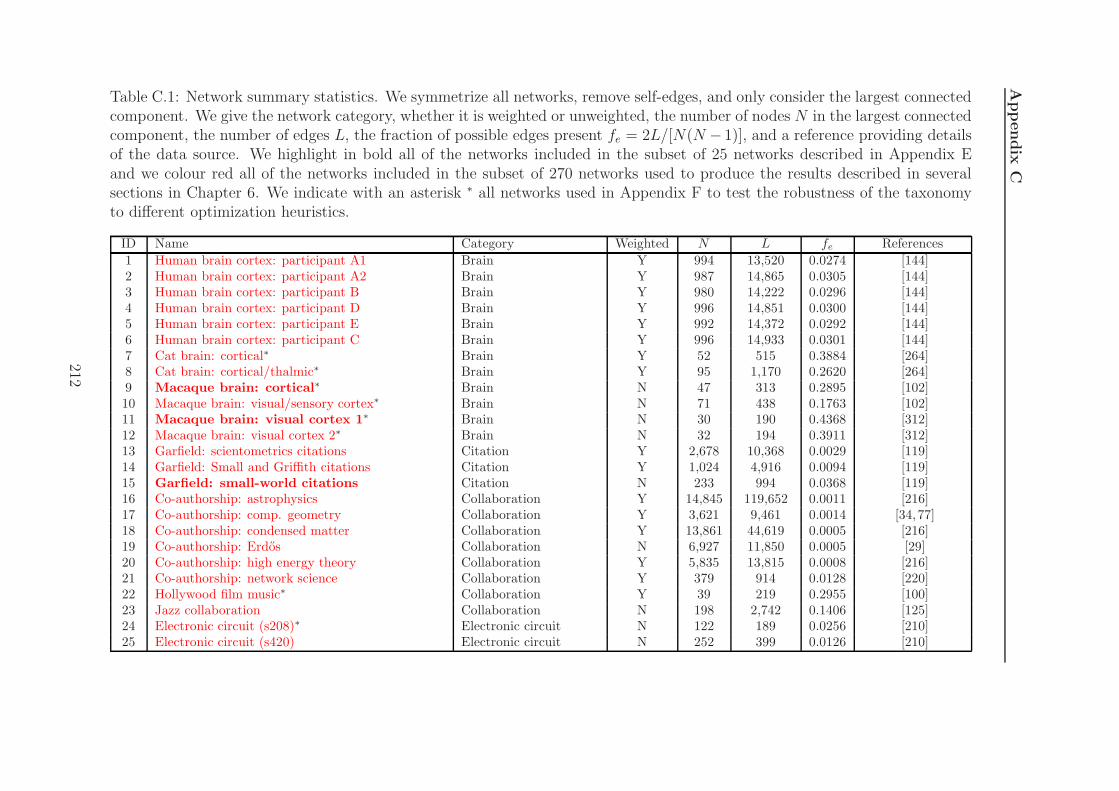
Appendix
CTable C.1: Network summary statistics. We symmetrize all networks, remove self-edges, and only consider the largest connectedcomponent. We give the network category, whether it is weighted or unweighted, the number of nodes N in the largest connectedcomponent, the number of edges L, the fraction of possible edges present fe = 2L/[N(N − 1)], and a reference providing detailsof the data source. We highlight in bold all of the networks included in the subset of 25 networks described in Appendix Eand we colour red all of the networks included in the subset of 270 networks used to produce the results described in severalsections in Chapter 6. We indicate with an asterisk ∗ all networks used in Appendix F to test the robustness of the taxonomyto different optimization heuristics.
ID Name Category Weighted N L fe References
1 Human brain cortex: participant A1 Brain Y 994 13,520 0.0274 [144]2 Human brain cortex: participant A2 Brain Y 987 14,865 0.0305 [144]3 Human brain cortex: participant B Brain Y 980 14,222 0.0296 [144]4 Human brain cortex: participant D Brain Y 996 14,851 0.0300 [144]5 Human brain cortex: participant E Brain Y 992 14,372 0.0292 [144]6 Human brain cortex: participant C Brain Y 996 14,933 0.0301 [144]7 Cat brain: cortical∗ Brain Y 52 515 0.3884 [264]8 Cat brain: cortical/thalmic∗ Brain Y 95 1,170 0.2620 [264]9 Macaque brain: cortical∗ Brain N 47 313 0.2895 [102]10 Macaque brain: visual/sensory cortex∗ Brain N 71 438 0.1763 [102]11 Macaque brain: visual cortex 1∗ Brain N 30 190 0.4368 [312]12 Macaque brain: visual cortex 2∗ Brain N 32 194 0.3911 [312]13 Garfield: scientometrics citations Citation Y 2,678 10,368 0.0029 [119]14 Garfield: Small and Griffith citations Citation Y 1,024 4,916 0.0094 [119]15 Garfield: small-world citations Citation N 233 994 0.0368 [119]16 Co-authorship: astrophysics Collaboration Y 14,845 119,652 0.0011 [216]17 Co-authorship: comp. geometry Collaboration Y 3,621 9,461 0.0014 [34, 77]18 Co-authorship: condensed matter Collaboration Y 13,861 44,619 0.0005 [216]19 Co-authorship: Erdos Collaboration N 6,927 11,850 0.0005 [29]20 Co-authorship: high energy theory Collaboration Y 5,835 13,815 0.0008 [216]21 Co-authorship: network science Collaboration Y 379 914 0.0128 [220]22 Hollywood film music∗ Collaboration Y 39 219 0.2955 [100]23 Jazz collaboration Collaboration N 198 2,742 0.1406 [125]24 Electronic circuit (s208)∗ Electronic circuit N 122 189 0.0256 [210]25 Electronic circuit (s420) Electronic circuit N 252 399 0.0126 [210]
212

Netw
ork
Deta
ils
ID Name Category Weighted N L fe References
26 Electronic circuit (s838) Electronic circuit N 512 819 0.0063 [210]27 Facebook: American Facebook N 6,370 217,654 0.0107 [295]28 Facebook: Amherst Facebook N 2,235 90,954 0.0364 [295]29 Facebook: Auburn Facebook N 18,448 973,918 0.0057 [295]30 Facebook: Baylor Facebook N 12,799 679,815 0.0083 [295]31 Facebook: BC Facebook N 11,498 486,961 0.0074 [295]32 Facebook: Berkeley Facebook N 22,900 852,419 0.0033 [295]33 Facebook: Bingham Facebook N 10,001 362,892 0.0073 [295]34 Facebook: Bowdoin Facebook N 2,250 84,386 0.0334 [295]35 Facebook: Brandeis Facebook N 3,887 137,561 0.0182 [295]36 Facebook: Brown Facebook N 8,586 384,519 0.0104 [295]37 Facebook: BU Facebook N 19,666 637,509 0.0033 [295]38 Facebook: Bucknell Facebook N 3,824 158,863 0.0217 [295]39 Facebook: Cal Facebook N 11,243 351,356 0.0056 [295]40 Facebook: Caltech Facebook N 762 16,651 0.0574 [295]41 Facebook: Carnegie Facebook N 6,621 249,959 0.0114 [295]42 Facebook: Colgate Facebook N 3,482 155,043 0.0256 [295]43 Facebook: Columbia Facebook N 11,706 444,295 0.0065 [295]44 Facebook: Cornell Facebook N 18,621 790,753 0.0046 [295]45 Facebook: Dartmouth Facebook N 7,677 304,065 0.0103 [295]46 Facebook: Duke Facebook N 9,885 506,437 0.0104 [295]47 Facebook: Emory Facebook N 7,449 330,008 0.0119 [295]48 Facebook: FSU Facebook N 27,731 1,034,799 0.0027 [295]49 Facebook: Georgetown Facebook N 9,388 425,619 0.0097 [295]50 Facebook: GWU Facebook N 12,164 469,511 0.0063 [295]51 Facebook: Hamilton Facebook N 2,312 96,393 0.0361 [295]52 Facebook: Harvard Facebook N 15,086 824,595 0.0072 [295]53 Facebook: Haverford Facebook N 1,446 59,589 0.0570 [295]54 Facebook: Howard Facebook N 4,047 204,850 0.0250 [295]55 Facebook: Indiana Facebook N 29,732 1,305,757 0.0030 [295]56 Facebook: JMU Facebook N 14,070 485,564 0.0049 [295]57 Facebook: Johns Hopkins Facebook N 5,157 186,572 0.0140 [295]58 Facebook: Lehigh Facebook N 5,073 198,346 0.0154 [295]59 Facebook: Maine Facebook N 9,065 243,245 0.0059 [295]60 Facebook: Maryland Facebook N 20,829 744,832 0.0034 [295]
213

Appendix
CID Name Category Weighted N L fe References
61 Facebook: Mich Facebook N 3,745 81,901 0.0117 [295]62 Facebook: Michigan Facebook N 30,106 1,176,489 0.0026 [295]63 Facebook: Middlebury Facebook N 3,069 124,607 0.0265 [295]64 Facebook: Mississippi Facebook N 10,519 610,910 0.0110 [295]65 Facebook: MIT Facebook N 6,402 251,230 0.0123 [295]66 Facebook: MSU Facebook N 32,361 1,118,767 0.0021 [295]67 Facebook: MU Facebook N 15,425 649,441 0.0055 [295]68 Facebook: Northeastern Facebook N 13,868 381,919 0.0040 [295]69 Facebook: Northwestern Facebook N 10,537 488,318 0.0088 [295]70 Facebook: Notre Dame Facebook N 12,149 541,336 0.0073 [295]71 Facebook: NYU Facebook Y 21,623 715,673 0.0031 [295]72 Facebook: Oberlin Facebook N 2,920 89,912 0.0211 [295]73 Facebook: Oklahoma Facebook N 17,420 892,524 0.0059 [295]74 Facebook: Penn Facebook N 41,536 1,362,220 0.0016 [295]75 Facebook: Pepperdine Facebook N 3,440 152,003 0.0257 [295]76 Facebook: Princeton Facebook N 6,575 293,307 0.0136 [295]77 Facebook: Reed Facebook N 962 18,812 0.0407 [295]78 Facebook: Rice Facebook N 4,083 184,826 0.0222 [295]79 Facebook: Rochester Facebook N 4,561 161,403 0.0155 [295]80 Facebook: Rutgers Facebook N 24,568 784,596 0.0026 [295]81 Facebook: Santa Facebook N 3,578 151,747 0.0237 [295]82 Facebook: Simmons Facebook N 1,510 32,984 0.0290 [295]83 Facebook: Smith Facebook N 2,970 97,133 0.0220 [295]84 Facebook: Stanford Facebook N 11,586 568,309 0.0085 [295]85 Facebook: Swarthmore Facebook N 1,657 61,049 0.0445 [295]86 Facebook: Syracuse Facebook N 13,640 543,975 0.0058 [295]87 Facebook: Temple Facebook N 13,653 360,774 0.0039 [295]88 Facebook: Tennessee Facebook N 16,977 770,658 0.0053 [295]89 Facebook: Texas80 Facebook N 31,538 1,219,639 0.0025 [295]90 Facebook: Texas84 Facebook N 36,364 1,590,651 0.0024 [295]91 Facebook: Trinity Facebook N 2,613 111,996 0.0328 [295]92 Facebook: Tufts Facebook N 6,672 249,722 0.0112 [295]93 Facebook: Tulane Facebook N 7,740 283,912 0.0095 [295]94 Facebook: U. Chicago Facebook N 6,561 208,088 0.0097 [295]95 Facebook: U. Conn. Facebook N 17,206 604,867 0.0041 [295]
214

Netw
ork
Deta
ils
ID Name Category Weighted N L fe References
96 Facebook: U. Illinois Facebook N 30,795 1,264,421 0.0027 [295]97 Facebook: U. Mass. Facebook N 16,502 519,376 0.0038 [295]98 Facebook: U. Penn. Facebook N 14,888 686,485 0.0062 [295]99 Facebook: UC33 Facebook N 16,800 522,141 0.0037 [295]100 Facebook: UC61 Facebook N 13,736 442,169 0.0047 [295]101 Facebook: UC64 Facebook N 6,810 155,320 0.0067 [295]102 Facebook: UCF Facebook N 14,936 428,987 0.0038 [295]103 Facebook: UCLA Facebook N 20,453 747,604 0.0036 [295]104 Facebook: UCSB Facebook N 14,917 482,215 0.0043 [295]105 Facebook: UCSC Facebook N 8,979 224,578 0.0056 [295]106 Facebook: UCSD Facebook N 14,936 443,215 0.0040 [295]107 Facebook: UF Facebook N 35,111 1,465,654 0.0024 [295]108 Facebook: UGA Facebook N 24,380 1,174,051 0.0040 [295]109 Facebook: UNC Facebook N 18,158 766,796 0.0047 [295]110 Facebook: USC Facebook N 17,440 801,851 0.0053 [295]111 Facebook: USF Facebook N 13,367 321,209 0.0036 [295]112 Facebook: USFCA Facebook N 2,672 65,244 0.0183 [295]113 Facebook: UVA Facebook N 17,178 789,308 0.0054 [295]114 Facebook: Vanderbilt Facebook N 8,063 427,829 0.0132 [295]115 Facebook: Vassar Facebook N 3,068 119,161 0.0253 [295]116 Facebook: Vermont Facebook N 7,322 191,220 0.0071 [295]117 Facebook: Villanova Facebook N 7,755 314,980 0.0105 [295]118 Facebook: Virginia Facebook N 21,319 698,175 0.0031 [295]119 Facebook: Wake Facebook N 5,366 279,186 0.0194 [295]120 Facebook: Wash. U. Facebook N 7,730 367,526 0.0123 [295]121 Facebook: Wellesley Facebook N 2,970 94,899 0.0215 [295]122 Facebook: Wesleyan Facebook N 3,591 138,034 0.0214 [295]123 Facebook: William Facebook N 6,472 266,378 0.0127 [295]124 Facebook: Williams Facebook N 2,788 112,985 0.0291 [295]125 Facebook: Wisconsin Facebook N 23,831 835,946 0.0029 [295]126 Facebook: Yale Facebook N 8,561 405,440 0.0111 [295]127 NYSE: 1980-1999 Financial Y 477 113,526 1.0000 [229]128 NYSE: 1980-1983 Financial Y 477 113,526 1.0000 [229]129 NYSE: 1984-1987 Financial Y 477 113,526 1.0000 [229]130 NYSE: 1988-1991 Financial Y 477 113,526 1.0000 [229]
215

Appendix
CID Name Category Weighted N L fe References
131 NYSE: 1992-1995 Financial Y 477 113,526 1.0000 [229]132 NYSE: 1996-1999 Financial Y 477 113,526 1.0000 [229]133 NYSE: H1 1985 Financial Y 100 4,950 1.0000 [1]134 NYSE: H2 1985 Financial Y 100 4,950 1.0000 [1]135 NYSE: H1 1986 Financial Y 100 4,950 1.0000 [1]136 NYSE: H2 1986 Financial Y 100 4,950 1.0000 [1]137 NYSE: H1 1987 Financial Y 100 4,950 1.0000 [1]138 NYSE: H2 1987 Financial Y 100 4,950 1.0000 [1]139 NYSE: H1 1988 Financial Y 100 4,950 1.0000 [1]140 NYSE: H2 1988 Financial Y 100 4,950 1.0000 [1]141 NYSE: H1 1989 Financial Y 100 4,950 1.0000 [1]142 NYSE: H2 1989 Financial Y 100 4,950 1.0000 [1]143 NYSE: H1 1990 Financial Y 100 4,950 1.0000 [1]144 NYSE: H2 1990 Financial Y 100 4,950 1.0000 [1]145 NYSE: H1 1991 Financial Y 100 4,950 1.0000 [1]146 NYSE: H2 1991 Financial Y 100 4,950 1.0000 [1]147 NYSE: H1 1992 Financial Y 100 4,950 1.0000 [1]148 NYSE: H2 1992 Financial Y 100 4,950 1.0000 [1]149 NYSE: H1 1993 Financial Y 100 4,950 1.0000 [1]150 NYSE: H2 1993 Financial Y 100 4,950 1.0000 [1]151 NYSE: H1 1994 Financial Y 100 4,950 1.0000 [1]152 NYSE: H2 1994 Financial Y 100 4,950 1.0000 [1]153 NYSE: H1 1995 Financial Y 100 4,950 1.0000 [1]154 NYSE: H2 1995 Financial Y 100 4,950 1.0000 [1]155 NYSE: H1 1996 Financial Y 100 4,950 1.0000 [1]156 NYSE: H2 1996 Financial Y 100 4,950 1.0000 [1]157 NYSE: H1 1997 Financial Y 100 4,950 1.0000 [1]158 NYSE: H2 1997 Financial Y 100 4,950 1.0000 [1]159 NYSE: H1 1998 Financial Y 100 4,950 1.0000 [1]160 NYSE: H2 1998 Financial Y 100 4,950 1.0000 [1]161 NYSE: H1 1999 Financial Y 100 4,950 1.0000 [1]162 NYSE: H2 1999 Financial Y 100 4,950 1.0000 [1]163 NYSE: H1 2000 Financial Y 100 4,950 1.0000 [1]164 NYSE: H2 2000 Financial Y 100 4,950 1.0000 [1]165 NYSE: H1 2001 Financial Y 100 4,950 1.0000 [1]
216
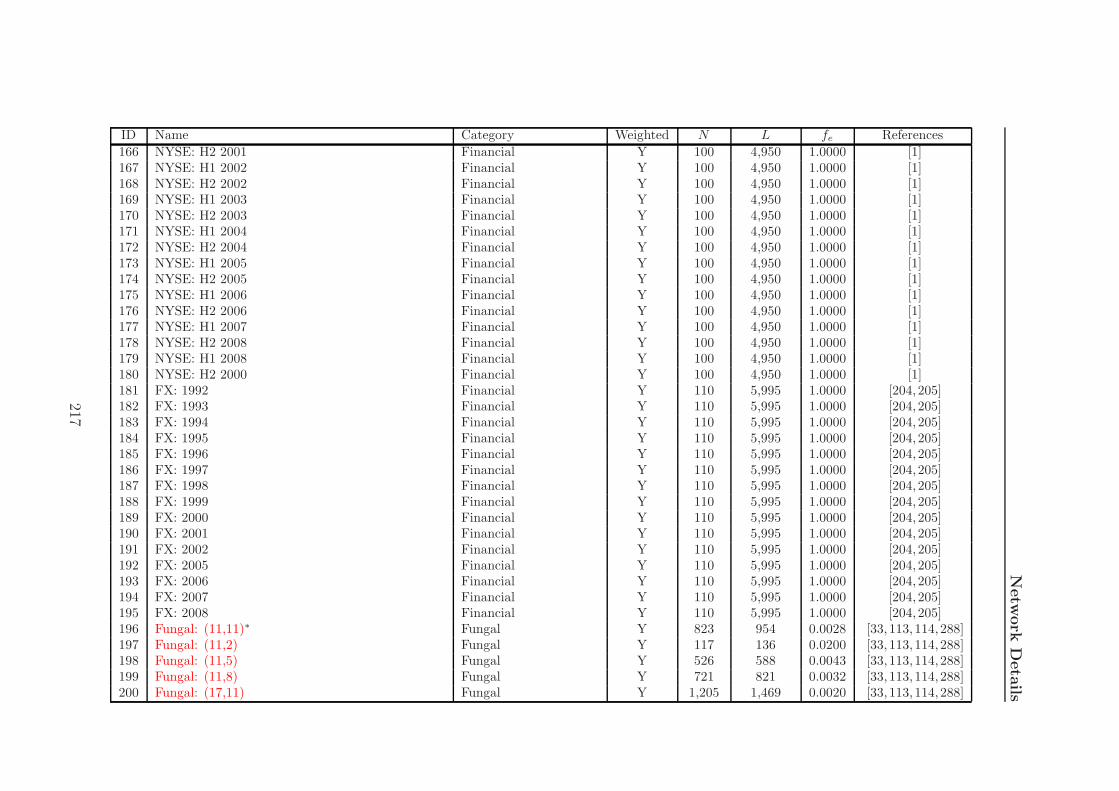
Netw
ork
Deta
ils
ID Name Category Weighted N L fe References
166 NYSE: H2 2001 Financial Y 100 4,950 1.0000 [1]167 NYSE: H1 2002 Financial Y 100 4,950 1.0000 [1]168 NYSE: H2 2002 Financial Y 100 4,950 1.0000 [1]169 NYSE: H1 2003 Financial Y 100 4,950 1.0000 [1]170 NYSE: H2 2003 Financial Y 100 4,950 1.0000 [1]171 NYSE: H1 2004 Financial Y 100 4,950 1.0000 [1]172 NYSE: H2 2004 Financial Y 100 4,950 1.0000 [1]173 NYSE: H1 2005 Financial Y 100 4,950 1.0000 [1]174 NYSE: H2 2005 Financial Y 100 4,950 1.0000 [1]175 NYSE: H1 2006 Financial Y 100 4,950 1.0000 [1]176 NYSE: H2 2006 Financial Y 100 4,950 1.0000 [1]177 NYSE: H1 2007 Financial Y 100 4,950 1.0000 [1]178 NYSE: H2 2008 Financial Y 100 4,950 1.0000 [1]179 NYSE: H1 2008 Financial Y 100 4,950 1.0000 [1]180 NYSE: H2 2000 Financial Y 100 4,950 1.0000 [1]181 FX: 1992 Financial Y 110 5,995 1.0000 [204,205]182 FX: 1993 Financial Y 110 5,995 1.0000 [204,205]183 FX: 1994 Financial Y 110 5,995 1.0000 [204,205]184 FX: 1995 Financial Y 110 5,995 1.0000 [204,205]185 FX: 1996 Financial Y 110 5,995 1.0000 [204,205]186 FX: 1997 Financial Y 110 5,995 1.0000 [204,205]187 FX: 1998 Financial Y 110 5,995 1.0000 [204,205]188 FX: 1999 Financial Y 110 5,995 1.0000 [204,205]189 FX: 2000 Financial Y 110 5,995 1.0000 [204,205]190 FX: 2001 Financial Y 110 5,995 1.0000 [204,205]191 FX: 2002 Financial Y 110 5,995 1.0000 [204,205]192 FX: 2005 Financial Y 110 5,995 1.0000 [204,205]193 FX: 2006 Financial Y 110 5,995 1.0000 [204,205]194 FX: 2007 Financial Y 110 5,995 1.0000 [204,205]195 FX: 2008 Financial Y 110 5,995 1.0000 [204,205]196 Fungal: (11,11)∗ Fungal Y 823 954 0.0028 [33, 113,114,288]197 Fungal: (11,2) Fungal Y 117 136 0.0200 [33, 113,114,288]198 Fungal: (11,5) Fungal Y 526 588 0.0043 [33, 113,114,288]199 Fungal: (11,8) Fungal Y 721 821 0.0032 [33, 113,114,288]200 Fungal: (17,11) Fungal Y 1,205 1,469 0.0020 [33, 113,114,288]
217

Appendix
CID Name Category Weighted N L fe References
201 Fungal: (17,2) Fungal Y 232 240 0.0090 [33, 113,114,288]202 Fungal: (17,5) Fungal Y 816 874 0.0026 [33, 113,114,288]203 Fungal: (17,8) Fungal Y 1,113 1,303 0.0021 [33, 113,114,288]204 Fungal: (4,11) Fungal Y 2,190 2,431 0.0010 [33, 113,114,288]205 Fungal: (4,2) Fungal Y 461 490 0.0046 [33, 113,114,288]206 Fungal: (4,5) Fungal Y 1,380 1,476 0.0016 [33, 113,114,288]207 Fungal: (4,8) Fungal Y 1,869 2,061 0.0012 [33, 113,114,288]208 AIDS blogs∗ WWW N 146 180 0.0170 [132]209 Political blogs WWW Y 1,222 16,714 0.0224 [3]210 WWW (Stanford) WWW N 8,929 26,320 0.0007 [124]211 Online Dictionary of Computing Language Y 13,356 91,471 0.0010 [30]212 Online Dictionary Of Information Science Language Y 2,898 16,376 0.0039 [77, 255]213 Reuters 9/11 news Language Y 13,308 148,035 0.0017 [158]214 Roget’s thesaurus Language N 994 3,640 0.0074 [77, 168]215 Word adjacency: English Language N 7,377 44,205 0.0016 [210]216 Word adjacency: French Language N 8,308 23,832 0.0007 [210]217 Word adjacency: Japanese Language N 2,698 7,995 0.0022 [210]218 Word adjacency: Spanish Language N 11,558 43,050 0.0006 [210]219 Metabolic: AA Metabolic N 411 1,818 0.0216 [156]220 Metabolic: AB Metabolic N 386 1,691 0.0228 [156]221 Metabolic: AG Metabolic N 494 2,173 0.0178 [156]222 Metabolic: AP Metabolic N 201 857 0.0426 [156]223 Metabolic: AT Metabolic N 296 1,231 0.0282 [156]224 Metabolic: BB Metabolic N 175 628 0.0412 [156]225 Metabolic: BS Metabolic N 772 3,611 0.0121 [156]226 Metabolic: CA Metabolic N 483 2,274 0.0195 [156]227 Metabolic: CE Metabolic N 453 2,025 0.0198 [156]228 Metabolic: CJ Metabolic N 370 1,631 0.0239 [156]229 Metabolic: CL Metabolic N 382 1,646 0.0226 [156]230 Metabolic: CQ Metabolic N 187 663 0.0381 [156]231 Metabolic: CT Metabolic N 211 772 0.0348 [156]232 Metabolic: CY Metabolic N 537 2,503 0.0174 [156]233 Metabolic: DR Metabolic N 800 3,789 0.0119 [156]234 Metabolic: EC Metabolic N 762 3,683 0.0127 [156]235 Metabolic: EF Metabolic N 375 1,721 0.0245 [156]
218

Netw
ork
Deta
ils
ID Name Category Weighted N L fe References
236 Metabolic: EN Metabolic N 374 1,617 0.0232 [156]237 Metabolic: HI Metabolic N 505 2,325 0.0183 [156]238 Metabolic: HP Metabolic N 365 1,703 0.0256 [156]239 Metabolic: MB Metabolic N 418 1,850 0.0212 [156]240 Metabolic: MG Metabolic N 199 783 0.0397 [156]241 Metabolic: MJ Metabolic N 422 1,874 0.0211 [156]242 Metabolic: ML Metabolic N 414 1,862 0.0218 [156]243 Metabolic: MP Metabolic N 171 685 0.0471 [156]244 Metabolic: MT Metabolic N 577 2,653 0.0160 [156]245 Metabolic: NG Metabolic N 394 1,824 0.0236 [156]246 Metabolic: NM Metabolic N 369 1,708 0.0252 [156]247 Metabolic: OS Metabolic N 285 1,168 0.0289 [156]248 Metabolic: PA Metabolic N 720 3,429 0.0132 [156]249 Metabolic: PF Metabolic N 310 1,379 0.0288 [156]250 Metabolic: PG Metabolic N 412 1,772 0.0209 [156]251 Metabolic: PH Metabolic N 318 1,394 0.0277 [156]252 Metabolic: PN Metabolic N 405 1,829 0.0224 [156]253 Metabolic: RC Metabolic N 663 3,111 0.0142 [156]254 Metabolic: RP Metabolic N 203 775 0.0378 [156]255 Metabolic: SC Metabolic N 552 2,595 0.0171 [156]256 Metabolic: ST Metabolic N 391 1,756 0.0230 [156]257 Metabolic: TH Metabolic N 427 1,955 0.0215 [156]258 Metabolic: TM Metabolic N 328 1,452 0.0271 [156]259 Metabolic: TP Metabolic N 194 788 0.0421 [156]260 Metabolic: TY Metabolic N 803 3,863 0.0120 [156]261 Metabolic: YP Metabolic N 552 2,471 0.0162 [156]262 U.S. political books co-purchase∗ Other N 105 441 0.0808 [171]263 Power grid Other N 4,941 6,594 0.0005 [305]264 Slovenian magazine co-purchase Other Y 124 5,972 0.7831 [28]265 Transcription: E. coli Other N 328 456 0.0085 [196]266 Transcription: Yeast Other N 662 1,062 0.0049 [211]267 U.S. airlines Other Y 324 2,081 0.0398 [29, 77]268 2008 NCAA football schedule∗ Other Y 121 764 0.1052 [61]269 Internet: autonomous systems Other N 22,963 48,436 0.0002 [219]270 Protein: serine protease inhibitor (1EAW)∗ Other N 53 123 0.0893 [210]
219

Appendix
CID Name Category Weighted N L fe References
271 Protein: immunoglobulin (1A4J)∗ Other N 95 213 0.0477 [210]272 Protein: oxidoreductase (1AOR)∗ Other N 97 212 0.0455 [210]273 Bill cosponsorship: U.S. House 96 Political: cosponsorship Y 438 95,529 0.9982 [108,109]274 Bill cosponsorship: U.S. House 97 Political: cosponsorship Y 435 94,374 0.9998 [108,109]275 Bill cosponsorship: U.S. House 98 Political: cosponsorship Y 437 95,256 0.9999 [108,109]276 Bill cosponsorship: U.S. House 99 Political: cosponsorship Y 437 94,999 0.9972 [108,109]277 Bill cosponsorship: U.S. House 100 Political: cosponsorship Y 439 96,125 0.9998 [108,109]278 Bill cosponsorship: U.S. House 101 Political: cosponsorship Y 437 95,263 1.0000 [108,109]279 Bill cosponsorship: U.S. House 102 Political: cosponsorship Y 437 95,051 0.9977 [108,109]280 Bill cosponsorship: U.S. House 103 Political: cosponsorship Y 437 95,028 0.9975 [108,109]281 Bill cosponsorship: U.S. House 104 Political: cosponsorship Y 439 95,925 0.9978 [108,109]282 Bill cosponsorship: U.S. House 105 Political: cosponsorship Y 442 97,373 0.9991 [108,109]283 Bill cosponsorship: U.S. House 106 Political: cosponsorship Y 436 94,820 0.9999 [108,109]284 Bill cosponsorship: U.S. House 107 Political: cosponsorship Y 442 97,233 0.9977 [108,109]285 Bill cosponsorship: U.S. House 108 Political: cosponsorship Y 439 96,104 0.9996 [108,109]286 Bill cosponsorship: U.S. Senate 96 Political: cosponsorship Y 101 5,050 1.0000 [108,109]287 Bill cosponsorship: U.S. Senate 97 Political: cosponsorship Y 101 5,050 1.0000 [108,109]288 Bill cosponsorship: U.S. Senate 98 Political: cosponsorship Y 101 5,050 1.0000 [108,109]289 Bill cosponsorship: U.S. Senate 99 Political: cosponsorship Y 101 5,049 0.9998 [108,109]290 Bill cosponsorship: U.S. Senate 100 Political: cosponsorship Y 101 5,050 1.0000 [108,109]291 Bill cosponsorship: U.S. Senate 101 Political: cosponsorship Y 100 4,950 1.0000 [108,109]292 Bill cosponsorship: U.S. Senate 102 Political: cosponsorship Y 102 5,142 0.9983 [108,109]293 Bill cosponsorship: U.S. Senate 103 Political: cosponsorship Y 101 5,050 1.0000 [108,109]294 Bill cosponsorship: U.S. Senate 104 Political: cosponsorship Y 102 5,151 1.0000 [108,109]295 Bill cosponsorship: U.S. Senate 105 Political: cosponsorship Y 100 4,950 1.0000 [108,109]296 Bill cosponsorship: U.S. Senate 106 Political: cosponsorship Y 102 5,151 1.0000 [108,109]297 Bill cosponsorship: U.S. Senate 107 Political: cosponsorship Y 101 5,049 0.9998 [108,109]298 Bill cosponsorship: U.S. Senate 108 Political: cosponsorship Y 100 4,950 1.0000 [108,109]299 Committees: U.S. House 101, comms. Political: committee N 159 3,610 0.2874 [242,243]300 Committees: U.S. House 102, comms. Political: committee N 163 4,093 0.3100 [242,243]301 Committees: U.S. House 103, comms. Political: committee N 141 2,983 0.3022 [242,243]302 Committees: U.S. House 104, comms. Political: committee N 106 1,839 0.3305 [242,243]303 Committees: U.S. House 105, comms. Political: committee N 108 1,997 0.3456 [242,243]304 Committees: U.S. House 106, comms. Political: committee N 107 2,031 0.3581 [242,243]305 Committees: U.S. House 107, comms. Political: committee N 113 2,429 0.3838 [242,243]
220

Netw
ork
Deta
ils
ID Name Category Weighted N L fe References
306 Committees: U.S. House 108, comms. Political: committee N 118 2,905 0.4208 [242,243]307 Committees: U.S. House 101, Reps. Political: committee N 434 18,714 0.1992 [242,243]308 Committees: U.S. House 102, Reps. Political: committee N 436 20,134 0.2123 [242,243]309 Committees: U.S. House 103, Reps. Political: committee N 437 18,212 0.1912 [242,243]310 Committees: U.S. House 104, Reps. Political: committee N 432 17,130 0.1840 [242,243]311 Committees: U.S. House 105, Reps. Political: committee N 435 18,297 0.1938 [242,243]312 Committees: U.S. House 106, Reps. Political: committee N 435 18,832 0.1995 [242,243]313 Committees: U.S. House 107, Reps. Political: committee N 434 19,824 0.2110 [242,243]314 Committees: U.S. House 108, Reps. Political: committee N 437 21,214 0.2227 [242,243]315 Roll call: U.S. House 1 Political: voting Y 66 2,122 0.9893 [203,241,306]316 Roll call: U.S. House 2 Political: voting Y 71 2,428 0.9771 [203,241,306]317 Roll call: U.S. House 3 Political: voting Y 108 5,669 0.9811 [203,241,306]318 Roll call: U.S. House 4 Political: voting Y 114 6,342 0.9846 [203,241,306]319 Roll call: U.S. House 5 Political: voting Y 117 6,600 0.9726 [203,241,306]320 Roll call: U.S. House 6 Political: voting Y 113 6,222 0.9832 [203,241,306]321 Roll call: U.S. House 7 Political: voting Y 110 5,921 0.9877 [203,241,306]322 Roll call: U.S. House 8 Political: voting Y 149 10,888 0.9875 [203,241,306]323 Roll call: U.S. House 9 Political: voting Y 147 10,582 0.9861 [203,241,306]324 Roll call: U.S. House 10 Political: voting Y 149 10,857 0.9847 [203,241,306]325 Roll call: U.S. House 11 Political: voting Y 153 11,482 0.9874 [203,241,306]326 Roll call: U.S. House 12 Political: voting Y 146 10,535 0.9953 [203,241,306]327 Roll call: U.S. House 13 Political: voting Y 195 18,723 0.9898 [203,241,306]328 Roll call: U.S. House 14 Political: voting Y 195 18,540 0.9802 [203,241,306]329 Roll call: U.S. House 15 Political: voting Y 195 18,666 0.9868 [203,241,306]330 Roll call: U.S. House 16 Political: voting Y 197 19,118 0.9903 [203,241,306]331 Roll call: U.S. House 17 Political: voting Y 199 19,429 0.9862 [203,241,306]332 Roll call: U.S. House 18 Political: voting Y 221 23,812 0.9795 [203,241,306]333 Roll call: U.S. House 19 Political: voting Y 220 23,993 0.9960 [203,241,306]334 Roll call: U.S. House 20 Political: voting Y 219 23,666 0.9914 [203,241,306]335 Roll call: U.S. House 21 Political: voting Y 220 23,985 0.9956 [203,241,306]336 Roll call: U.S. House 22 Political: voting Y 217 23,404 0.9986 [203,241,306]337 Roll call: U.S. House 23 Political: voting Y 257 32,502 0.9880 [203,241,306]338 Roll call: U.S. House 24 Political: voting Y 255 32,062 0.9900 [203,241,306]339 Roll call: U.S. House 25 Political: voting Y 256 32,366 0.9916 [203,241,306]340 Roll call: U.S. House 26 Political: voting Y 255 32,067 0.9902 [203,241,306]
221

Appendix
CID Name Category Weighted N L fe References
341 Roll call: U.S. House 27 Political: voting Y 257 32,743 0.9953 [203,241,306]342 Roll call: U.S. House 28 Political: voting Y 234 26,788 0.9826 [203,241,306]343 Roll call: U.S. House 29 Political: voting Y 236 27,562 0.9939 [203,241,306]344 Roll call: U.S. House 30 Political: voting Y 236 27,669 0.9978 [203,241,306]345 Roll call: U.S. House 31 Political: voting Y 241 28,804 0.9960 [203,241,306]346 Roll call: U.S. House 32 Political: voting Y 239 28,318 0.9957 [203,241,306]347 Roll call: U.S. House 33 Political: voting Y 240 28,570 0.9962 [203,241,306]348 Roll call: U.S. House 34 Political: voting Y 236 27,545 0.9933 [203,241,306]349 Roll call: U.S. House 35 Political: voting Y 245 29,630 0.9913 [203,241,306]350 Roll call: U.S. House 36 Political: voting Y 243 29,312 0.9969 [203,241,306]351 Roll call: U.S. House 37 Political: voting Y 197 18,735 0.9704 [203,241,306]352 Roll call: U.S. House 38 Political: voting Y 187 17,326 0.9963 [203,241,306]353 Roll call: U.S. House 39 Political: voting Y 199 19,593 0.9945 [203,241,306]354 Roll call: U.S. House 40 Political: voting Y 233 26,605 0.9843 [203,241,306]355 Roll call: U.S. House 41 Political: voting Y 256 32,109 0.9837 [203,241,306]356 Roll call: U.S. House 42 Political: voting Y 253 31,626 0.9921 [203,241,306]357 Roll call: U.S. House 43 Political: voting Y 302 45,151 0.9934 [203,241,306]358 Roll call: U.S. House 44 Political: voting Y 308 46,723 0.9883 [203,241,306]359 Roll call: U.S. House 45 Political: voting Y 302 45,315 0.9970 [203,241,306]360 Roll call: U.S. House 46 Political: voting Y 301 44,987 0.9964 [203,241,306]361 Roll call: U.S. House 47 Political: voting Y 306 46,214 0.9903 [203,241,306]362 Roll call: U.S. House 48 Political: voting Y 338 56,484 0.9918 [203,241,306]363 Roll call: U.S. House 49 Political: voting Y 330 54,160 0.9977 [203,241,306]364 Roll call: U.S. House 50 Political: voting Y 326 52,907 0.9987 [203,241,306]365 Roll call: U.S. House 51 Political: voting Y 347 59,303 0.9879 [203,241,306]366 Roll call: U.S. House 52 Political: voting Y 340 57,285 0.9940 [203,241,306]367 Roll call: U.S. House 53 Political: voting Y 376 69,943 0.9921 [203,241,306]368 Roll call: U.S. House 54 Political: voting Y 368 67,085 0.9934 [203,241,306]369 Roll call: U.S. House 55 Political: voting Y 371 68,270 0.9947 [203,241,306]370 Roll call: U.S. House 56 Political: voting Y 369 67,059 0.9877 [203,241,306]371 Roll call: U.S. House 57 Political: voting Y 371 67,383 0.9818 [203,241,306]372 Roll call: U.S. House 58 Political: voting Y 397 75,891 0.9655 [203,241,306]373 Roll call: U.S. House 59 Political: voting Y 397 76,299 0.9707 [203,241,306]374 Roll call: U.S. House 60 Political: voting Y 398 77,921 0.9863 [203,241,306]375 Roll call: U.S. House 61 Political: voting Y 402 80,174 0.9947 [203,241,306]
222

Netw
ork
Deta
ils
ID Name Category Weighted N L fe References
376 Roll call: U.S. House 62 Political: voting Y 408 82,442 0.9929 [203,241,306]377 Roll call: U.S. House 63 Political: voting Y 452 101,498 0.9958 [203,241,306]378 Roll call: U.S. House 64 Political: voting Y 441 96,780 0.9975 [203,241,306]379 Roll call: U.S. House 65 Political: voting Y 454 102,108 0.9930 [203,241,306]380 Roll call: U.S. House 66 Political: voting Y 453 101,199 0.9885 [203,241,306]381 Roll call: U.S. House 67 Political: voting Y 452 101,482 0.9956 [203,241,306]382 Roll call: U.S. House 68 Political: voting Y 442 96,885 0.9941 [203,241,306]383 Roll call: U.S. House 69 Political: voting Y 437 95,226 0.9996 [203,241,306]384 Roll call: U.S. House 70 Political: voting Y 443 97,497 0.9959 [203,241,306]385 Roll call: U.S. House 71 Political: voting Y 455 102,502 0.9924 [203,241,306]386 Roll call: U.S. House 72 Political: voting Y 447 99,028 0.9934 [203,241,306]387 Roll call: U.S. House 73 Political: voting Y 445 98,647 0.9986 [203,241,306]388 Roll call: U.S. House 74 Political: voting Y 440 96,170 0.9958 [203,241,306]389 Roll call: U.S. House 75 Political: voting Y 445 98,474 0.9968 [203,241,306]390 Roll call: U.S. House 76 Political: voting Y 456 102,495 0.9880 [203,241,306]391 Roll call: U.S. House 77 Political: voting Y 450 99,956 0.9894 [203,241,306]392 Roll call: U.S. House 78 Political: voting Y 450 100,513 0.9949 [203,241,306]393 Roll call: U.S. House 79 Political: voting Y 448 99,246 0.9912 [203,241,306]394 Roll call: U.S. House 80 Political: voting Y 448 99,902 0.9977 [203,241,306]395 Roll call: U.S. House 81 Political: voting Y 444 98,054 0.9970 [203,241,306]396 Roll call: U.S. House 82 Political: voting Y 447 99,281 0.9960 [203,241,306]397 Roll call: U.S. House 83 Political: voting Y 440 96,506 0.9992 [203,241,306]398 Roll call: U.S. House 84 Political: voting Y 437 95,253 0.9999 [203,241,306]399 Roll call: U.S. House 85 Political: voting Y 444 97,955 0.9960 [203,241,306]400 Roll call: U.S. House 86 Political: voting Y 443 97,377 0.9946 [203,241,306]401 Roll call: U.S. House 87 Political: voting Y 449 99,774 0.9920 [203,241,306]401 Roll call: U.S. House 88 Political: voting Y 443 97,842 0.9994 [203,241,306]403 Roll call: U.S. House 89 Political: voting Y 442 97,139 0.9967 [203,241,306]404 Roll call: U.S. House 90 Political: voting Y 437 95,251 0.9998 [203,241,306]405 Roll call: U.S. House 91 Political: voting Y 448 99,815 0.9969 [203,241,306]406 Roll call: U.S. House 92 Political: voting Y 443 97,579 0.9967 [203,241,306]407 Roll call: U.S. House 93 Political: voting Y 443 97,848 0.9994 [203,241,306]408 Roll call: U.S. House 94 Political: voting Y 441 96,837 0.9981 [203,241,306]409 Roll call: U.S. House 95 Political: voting Y 441 96,493 0.9946 [203,241,306]410 Roll call: U.S. House 96 Political: voting Y 440 96,379 0.9979 [203,241,306]
223

Appendix
CID Name Category Weighted N L fe References
411 Roll call: U.S. House 97 Political: voting Y 442 96,761 0.9928 [203,241,306]412 Roll call: U.S. House 98 Political: voting Y 439 95,922 0.9977 [203,241,306]413 Roll call: U.S. House 99 Political: voting Y 439 95,875 0.9972 [203,241,306]414 Roll call: U.S. House 100 Political: voting Y 440 96,544 0.9996 [203,241,306]415 Roll call: U.S. House 101 Political: voting Y 440 96,505 0.9992 [203,241,306]416 Roll call: U.S. House 102 Political: voting Y 441 96,811 0.9978 [203,241,306]417 Roll call: U.S. House 103 Political: voting Y 441 96,348 0.9931 [203,241,306]418 Roll call: U.S. House 104 Political: voting Y 445 98,720 0.9993 [203,241,306]419 Roll call: U.S. House 105 Political: voting Y 443 97,841 0.9994 [203,241,306]420 Roll call: U.S. House 106 Political: voting Y 440 96,557 0.9998 [203,241,306]421 Roll call: U.S. House 107 Political: voting Y 443 97,816 0.9991 [203,241,306]422 Roll call: U.S. House 108 Political: voting Y 440 96,561 0.9998 [203,241,306]423 Roll call: U.S. House 109 Political: voting Y 440 96,549 0.9997 [203,241,306]424 Roll call: U.S. House 110 Political: voting Y 448 99,603 0.9948 [203,241,306]425 Roll call: U.S. Senate 1 Political: voting Y 29 393 0.9680 [203,241,306]426 Roll call: U.S. Senate 2 Political: voting Y 31 449 0.9656 [203,241,306]427 Roll call: U.S. Senate 3 Political: voting Y 32 472 0.9516 [203,241,306]428 Roll call: U.S. Senate 4 Political: voting Y 43 760 0.8416 [203,241,306]429 Roll call: U.S. Senate 5 Political: voting Y 44 808 0.8541 [203,241,306]430 Roll call: U.S. Senate 6 Political: voting Y 37 644 0.9670 [203,241,306]431 Roll call: U.S. Senate 7 Political: voting Y 35 537 0.9025 [203,241,306]432 Roll call: U.S. Senate 8 Political: voting Y 44 864 0.9133 [203,241,306]433 Roll call: U.S. Senate 9 Political: voting Y 37 645 0.9685 [203,241,306]434 Roll call: U.S. Senate 10 Political: voting Y 37 660 0.9910 [203,241,306]435 Roll call: U.S. Senate 11 Political: voting Y 44 855 0.9038 [203,241,306]436 Roll call: U.S. Senate 12 Political: voting Y 37 663 0.9955 [203,241,306]437 Roll call: U.S. Senate 13 Political: voting Y 46 947 0.9150 [203,241,306]438 Roll call: U.S. Senate 14 Political: voting Y 44 898 0.9493 [203,241,306]439 Roll call: U.S. Senate 15 Political: voting Y 46 977 0.9440 [203,241,306]440 Roll call: U.S. Senate 16 Political: voting Y 51 1,249 0.9796 [203,241,306]441 Roll call: U.S. Senate 17 Political: voting Y 52 1,294 0.9759 [203,241,306]442 Roll call: U.S. Senate 18 Political: voting Y 52 1,304 0.9834 [203,241,306]443 Roll call: U.S. Senate 19 Political: voting Y 59 1,589 0.9287 [203,241,306]444 Roll call: U.S. Senate 20 Political: voting Y 53 1,343 0.9746 [203,241,306]445 Roll call: U.S. Senate 21 Political: voting Y 54 1,339 0.9357 [203,241,306]
224

Netw
ork
Deta
ils
ID Name Category Weighted N L fe References
446 Roll call: U.S. Senate 22 Political: voting Y 53 1,348 0.9782 [203,241,306]447 Roll call: U.S. Senate 23 Political: voting Y 54 1,378 0.9630 [203,241,306]448 Roll call: U.S. Senate 24 Political: voting Y 61 1,732 0.9464 [203,241,306]449 Roll call: U.S. Senate 25 Political: voting Y 58 1,627 0.9843 [203,241,306]440 Roll call: U.S. Senate 26 Political: voting Y 60 1,689 0.9542 [203,241,306]451 Roll call: U.S. Senate 27 Political: voting Y 59 1,662 0.9714 [203,241,306]452 Roll call: U.S. Senate 28 Political: voting Y 57 1,575 0.9868 [203,241,306]453 Roll call: U.S. Senate 29 Political: voting Y 63 1,895 0.9703 [203,241,306]454 Roll call: U.S. Senate 30 Political: voting Y 72 2,320 0.9077 [203,241,306]455 Roll call: U.S. Senate 31 Political: voting Y 70 2,341 0.9694 [203,241,306]456 Roll call: U.S. Senate 32 Political: voting Y 73 2,511 0.9555 [203,241,306]457 Roll call: U.S. Senate 33 Political: voting Y 70 2,308 0.9557 [203,241,306]458 Roll call: U.S. Senate 34 Political: voting Y 64 2,002 0.9931 [203,241,306]459 Roll call: U.S. Senate 35 Political: voting Y 73 2,542 0.9673 [203,241,306]460 Roll call: U.S. Senate 36 Political: voting Y 70 2,370 0.9814 [203,241,306]461 Roll call: U.S. Senate 37 Political: voting Y 70 2,051 0.8493 [203,241,306]462 Roll call: U.S. Senate 38 Political: voting Y 54 1,402 0.9797 [203,241,306]463 Roll call: U.S. Senate 39 Political: voting Y 59 1,610 0.9410 [203,241,306]464 Roll call: U.S. Senate 40 Political: voting Y 69 2,274 0.9693 [203,241,306]465 Roll call: U.S. Senate 41 Political: voting Y 80 3,084 0.9759 [203,241,306]466 Roll call: U.S. Senate 42 Political: voting Y 75 2,773 0.9993 [203,241,306]467 Roll call: U.S. Senate 43 Political: voting Y 79 3,041 0.9870 [203,241,306]468 Roll call: U.S. Senate 44 Political: voting Y 82 3,261 0.9819 [203,241,306]469 Roll call: U.S. Senate 45 Political: voting Y 82 3,265 0.9831 [203,241,306]470 Roll call: U.S. Senate 46 Political: voting Y 81 3,219 0.9935 [203,241,306]471 Roll call: U.S. Senate 47 Political: voting Y 83 3,362 0.9880 [203,241,306]472 Roll call: U.S. Senate 48 Political: voting Y 78 2,998 0.9983 [203,241,306]473 Roll call: U.S. Senate 49 Political: voting Y 81 3,210 0.9907 [203,241,306]474 Roll call: U.S. Senate 50 Political: voting Y 76 2,850 1.0000 [203,241,306]475 Roll call: U.S. Senate 51 Political: voting Y 91 3,998 0.9763 [203,241,306]476 Roll call: U.S. Senate 52 Political: voting Y 93 4,249 0.9932 [203,241,306]477 Roll call: U.S. Senate 53 Political: voting Y 95 4,413 0.9884 [203,241,306]478 Roll call: U.S. Senate 54 Political: voting Y 90 4,000 0.9988 [203,241,306]479 Roll call: U.S. Senate 55 Political: voting Y 96 4,445 0.9748 [203,241,306]480 Roll call: U.S. Senate 56 Political: voting Y 93 4,201 0.9820 [203,241,306]
225

Appendix
CID Name Category Weighted N L fe References
481 Roll call: U.S. Senate 57 Political: voting Y 90 3,939 0.9835 [203,241,306]482 Roll call: U.S. Senate 58 Political: voting Y 93 4,174 0.9757 [203,241,306]483 Roll call: U.S. Senate 59 Political: voting Y 93 4,251 0.9937 [203,241,306]484 Roll call: U.S. Senate 60 Political: voting Y 95 4,382 0.9814 [203,241,306]485 Roll call: U.S. Senate 61 Political: voting Y 102 5,033 0.9771 [203,241,306]486 Roll call: U.S. Senate 62 Political: voting Y 109 5,719 0.9716 [203,241,306]487 Roll call: U.S. Senate 63 Political: voting Y 101 5,029 0.9958 [203,241,306]488 Roll call: U.S. Senate 64 Political: voting Y 100 4,931 0.9962 [203,241,306]489 Roll call: U.S. Senate 65 Political: voting Y 111 5,899 0.9663 [203,241,306]490 Roll call: U.S. Senate 66 Political: voting Y 101 5,005 0.9911 [203,241,306]491 Roll call: U.S. Senate 67 Political: voting Y 105 5,413 0.9914 [203,241,306]492 Roll call: U.S. Senate 68 Political: voting Y 102 5,081 0.9864 [203,241,306]493 Roll call: U.S. Senate 69 Political: voting Y 105 5,353 0.9804 [203,241,306]494 Roll call: U.S. Senate 70 Political: voting Y 102 5,082 0.9866 [203,241,306]495 Roll call: U.S. Senate 71 Political: voting Y 109 5,779 0.9818 [203,241,306]496 Roll call: U.S. Senate 72 Political: voting Y 103 5,220 0.9937 [203,241,306]497 Roll call: U.S. Senate 73 Political: voting Y 100 4,879 0.9857 [203,241,306]498 Roll call: U.S. Senate 74 Political: voting Y 100 4,933 0.9966 [203,241,306]499 Roll call: U.S. Senate 75 Political: voting Y 102 5,126 0.9951 [203,241,306]500 Roll call: U.S. Senate 76 Political: voting Y 104 5,106 0.9533 [203,241,306]501 Roll call: U.S. Senate 77 Political: voting Y 108 5,575 0.9649 [203,241,306]502 Roll call: U.S. Senate 78 Political: voting Y 104 5,304 0.9903 [203,241,306]503 Roll call: U.S. Senate 79 Political: voting Y 107 5,466 0.9639 [203,241,306]504 Roll call: U.S. Senate 80 Political: voting Y 97 4,655 0.9998 [203,241,306]505 Roll call: U.S. Senate 81 Political: voting Y 108 5,646 0.9772 [203,241,306]506 Roll call: U.S. Senate 82 Political: voting Y 98 4,748 0.9989 [203,241,306]507 Roll call: U.S. Senate 83 Political: voting Y 110 5,724 0.9548 [203,241,306]508 Roll call: U.S. Senate 84 Political: voting Y 99 4,845 0.9988 [203,241,306]509 Roll call: U.S. Senate 85 Political: voting Y 101 5,014 0.9929 [203,241,306]510 Roll call: U.S. Senate 86 Political: voting Y 103 5,246 0.9987 [203,241,306]511 Roll call: U.S. Senate 87 Political: voting Y 105 5,444 0.9971 [203,241,306]512 Roll call: U.S. Senate 88 Political: voting Y 103 5,249 0.9992 [203,241,306]513 Roll call: U.S. Senate 89 Political: voting Y 103 5,247 0.9989 [203,241,306]514 Roll call: U.S. Senate 90 Political: voting Y 101 5,048 0.9996 [203,241,306]515 Roll call: U.S. Senate 91 Political: voting Y 102 5,148 0.9994 [203,241,306]
226
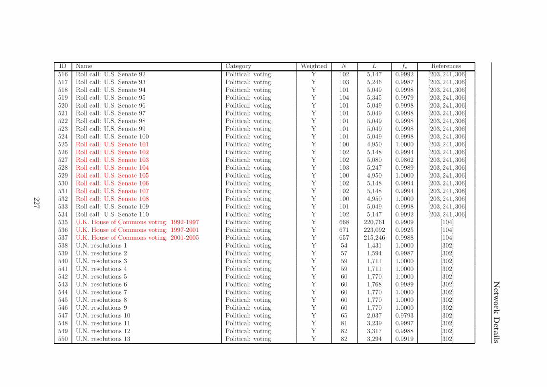
Netw
ork
Deta
ils
ID Name Category Weighted N L fe References
516 Roll call: U.S. Senate 92 Political: voting Y 102 5,147 0.9992 [203,241,306]517 Roll call: U.S. Senate 93 Political: voting Y 103 5,246 0.9987 [203,241,306]518 Roll call: U.S. Senate 94 Political: voting Y 101 5,049 0.9998 [203,241,306]519 Roll call: U.S. Senate 95 Political: voting Y 104 5,345 0.9979 [203,241,306]520 Roll call: U.S. Senate 96 Political: voting Y 101 5,049 0.9998 [203,241,306]521 Roll call: U.S. Senate 97 Political: voting Y 101 5,049 0.9998 [203,241,306]522 Roll call: U.S. Senate 98 Political: voting Y 101 5,049 0.9998 [203,241,306]523 Roll call: U.S. Senate 99 Political: voting Y 101 5,049 0.9998 [203,241,306]524 Roll call: U.S. Senate 100 Political: voting Y 101 5,049 0.9998 [203,241,306]525 Roll call: U.S. Senate 101 Political: voting Y 100 4,950 1.0000 [203,241,306]526 Roll call: U.S. Senate 102 Political: voting Y 102 5,148 0.9994 [203,241,306]527 Roll call: U.S. Senate 103 Political: voting Y 102 5,080 0.9862 [203,241,306]528 Roll call: U.S. Senate 104 Political: voting Y 103 5,247 0.9989 [203,241,306]529 Roll call: U.S. Senate 105 Political: voting Y 100 4,950 1.0000 [203,241,306]530 Roll call: U.S. Senate 106 Political: voting Y 102 5,148 0.9994 [203,241,306]531 Roll call: U.S. Senate 107 Political: voting Y 102 5,148 0.9994 [203,241,306]532 Roll call: U.S. Senate 108 Political: voting Y 100 4,950 1.0000 [203,241,306]533 Roll call: U.S. Senate 109 Political: voting Y 101 5,049 0.9998 [203,241,306]534 Roll call: U.S. Senate 110 Political: voting Y 102 5,147 0.9992 [203,241,306]535 U.K. House of Commons voting: 1992-1997 Political: voting Y 668 220,761 0.9909 [104]536 U.K. House of Commons voting: 1997-2001 Political: voting Y 671 223,092 0.9925 [104]537 U.K. House of Commons voting: 2001-2005 Political: voting Y 657 215,246 0.9988 [104]538 U.N. resolutions 1 Political: voting Y 54 1,431 1.0000 [302]539 U.N. resolutions 2 Political: voting Y 57 1,594 0.9987 [302]540 U.N. resolutions 3 Political: voting Y 59 1,711 1.0000 [302]541 U.N. resolutions 4 Political: voting Y 59 1,711 1.0000 [302]542 U.N. resolutions 5 Political: voting Y 60 1,770 1.0000 [302]543 U.N. resolutions 6 Political: voting Y 60 1,768 0.9989 [302]544 U.N. resolutions 7 Political: voting Y 60 1,770 1.0000 [302]545 U.N. resolutions 8 Political: voting Y 60 1,770 1.0000 [302]546 U.N. resolutions 9 Political: voting Y 60 1,770 1.0000 [302]547 U.N. resolutions 10 Political: voting Y 65 2,037 0.9793 [302]548 U.N. resolutions 11 Political: voting Y 81 3,239 0.9997 [302]549 U.N. resolutions 12 Political: voting Y 82 3,317 0.9988 [302]550 U.N. resolutions 13 Political: voting Y 82 3,294 0.9919 [302]
227

Appendix
CID Name Category Weighted N L fe References
551 U.N. resolutions 14 Political: voting Y 82 3,321 1.0000 [302]552 U.N. resolutions 15 Political: voting Y 99 4,851 1.0000 [302]553 U.N. resolutions 16 Political: voting Y 104 5,356 1.0000 [302]554 U.N. resolutions 17 Political: voting Y 110 5,995 1.0000 [302]555 U.N. resolutions 18 Political: voting Y 113 6,246 0.9870 [302]556 U.N. resolutions 20 Political: voting Y 117 6,672 0.9832 [302]557 U.N. resolutions 21 Political: voting Y 122 7,333 0.9935 [302]558 U.N. resolutions 22 Political: voting Y 124 7,616 0.9987 [302]559 U.N. resolutions 23 Political: voting Y 126 7,855 0.9975 [302]560 U.N. resolutions 24 Political: voting Y 126 7,851 0.9970 [302]561 U.N. resolutions 25 Political: voting Y 126 7,868 0.9991 [302]562 U.N. resolutions 26 Political: voting Y 132 8,641 0.9994 [302]563 U.N. resolutions 27 Political: voting Y 132 8,646 1.0000 [302]564 U.N. resolutions 28 Political: voting Y 134 8,905 0.9993 [302]565 U.N. resolutions 29 Political: voting Y 137 9,202 0.9878 [302]566 U.N. resolutions 30 Political: voting Y 143 10,117 0.9965 [302]567 U.N. resolutions 31 Political: voting Y 144 10,291 0.9995 [302]568 U.N. resolutions 32 Political: voting Y 146 10,585 1.0000 [302]569 U.N. resolutions 33 Political: voting Y 148 10,878 1.0000 [302]570 U.N. resolutions 34 Political: voting Y 150 11,173 0.9998 [302]571 U.N. resolutions 35 Political: voting Y 151 11,287 0.9966 [302]572 U.N. resolutions 36 Political: voting Y 155 11,935 1.0000 [302]573 U.N. resolutions 37 Political: voting Y 156 12,090 1.0000 [302]574 U.N. resolutions 38 Political: voting Y 157 12,243 0.9998 [302]575 U.N. resolutions 39 Political: voting Y 158 12,403 1.0000 [302]576 U.N. resolutions 40 Political: voting Y 158 12,403 1.0000 [302]577 U.N. resolutions 41 Political: voting Y 158 12,403 1.0000 [302]578 U.N. resolutions 42 Political: voting Y 158 12,402 0.9999 [302]579 U.N. resolutions 43 Political: voting Y 158 12,403 1.0000 [302]580 U.N. resolutions 44 Political: voting Y 158 12,403 1.0000 [302]581 U.N. resolutions 45 Political: voting Y 154 11,781 1.0000 [302]582 U.N. resolutions 46 Political: voting Y 168 13,872 0.9889 [302]583 U.N. resolutions 47 Political: voting Y 174 14,944 0.9929 [302]584 U.N. resolutions 48 Political: voting Y 178 15,606 0.9907 [302]585 U.N. resolutions 49 Political: voting Y 174 14,913 0.9908 [302]
228

Netw
ork
Deta
ils
ID Name Category Weighted N L fe References
586 U.N. resolutions 50 Political: voting Y 179 15,826 0.9934 [302]587 U.N. resolutions 51 Political: voting Y 180 16,096 0.9991 [302]588 U.N. resolutions 52 Political: voting Y 176 15,349 0.9967 [302]589 U.N. resolutions 53 Political: voting Y 177 15,500 0.9951 [302]590 U.N. resolutions 54 Political: voting Y 174 14,970 0.9946 [302]591 U.N. resolutions 55 Political: voting Y 182 16,333 0.9916 [302]592 U.N. resolutions 56 Political: voting Y 179 15,812 0.9925 [302]593 U.N. resolutions 57 Political: voting Y 187 17,373 0.9990 [302]594 U.N. resolutions 58 Political: voting Y 189 17,735 0.9983 [302]595 U.N. resolutions 59 Political: voting Y 191 18,140 0.9997 [302]596 U.N. resolutions 60 Political: voting Y 191 18,110 0.9981 [302]597 U.N. resolutions 61 Political: voting Y 192 18,331 0.9997 [302]598 U.N. resolutions 62 Political: voting Y 192 18,331 0.9997 [302]599 U.N. resolutions 63 Political: voting Y 192 18,328 0.9996 [302]600 Biogrid: A. thaliana Protein interaction N 406 625 0.0076 [280]601 Biogrid: C. elegans Protein interaction N 3,353 6,449 0.0011 [280]602 Biogrid: D. melanogaster Protein interaction N 7,174 24,897 0.0010 [280]603 Biogrid: H. sapien Protein interaction N 8,205 25,699 0.0008 [280]604 Biogrid: M. musculus Protein interaction N 710 1,003 0.0040 [280]605 Biogrid: R. norvegicus∗ Protein interaction N 121 135 0.0186 [280]606 Biogrid: S. cerevisiae Protein interaction N 1,753 4,811 0.0031 [280]607 Biogrid: S. pombe Protein interaction N 1,477 11,404 0.0105 [280]608 DIP: H. pylori Protein interaction N 686 1,351 0.0058 [262,310]609 DIP: H. sapien Protein interaction N 639 982 0.0048 [262,310]610 DIP: M. musculus Protein interaction N 50 55 0.0449 [262,310]611 DIP: C. elegans Protein interaction N 2,386 3,825 0.0013 [262,310]612 Human: Ccsb Protein interaction N 1,307 2,483 0.0029 [261]613 Human: Ophid Protein interaction N 5,464 23,238 0.0016 [57, 58]614 STRING: C. elegans Protein interaction N 1,762 95,227 0.0614 [155]615 STRING: S. cerevisiae Protein interaction N 534 57,672 0.4053 [155]616 Yeast: Oxford Statistics Protein interaction N 2,224 6,609 0.0027 [67]617 Yeast: DIP Protein interaction N 4,906 17,218 0.0014 [4, 262,310]618 Yeast: DIPC Protein interaction N 2,587 6,094 0.0018 [4, 262,310]619 Yeast: FHC Protein interaction N 2,233 5,750 0.0023 [4, 43]620 Yeast: FYI Protein interaction N 778 1,798 0.0059 [4, 146]
229
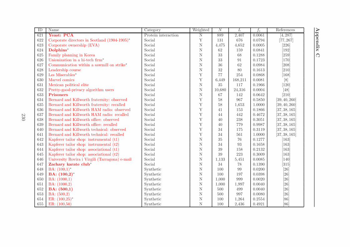
Appendix
CID Name Category Weighted N L fe References
621 Yeast: PCA Protein interaction N 889 2,407 0.0061 [4, 287]622 Corporate directors in Scotland (1904-1905)∗ Social Y 131 676 0.0794 [77, 267]623 Corporate ownership (EVA) Social N 4,475 4,652 0.0005 [226]624 Dolphins∗ Social N 62 159 0.0841 [192]625 Family planning in Korea Social N 33 68 0.1288 [259]626 Unionization in a hi-tech firm∗ Social N 33 91 0.1723 [170]627 Communication within a sawmill on strike∗ Social N 36 62 0.0984 [208]628 Leadership course Social N 32 80 0.1613 [210]629 Les Miserables∗ Social Y 77 254 0.0868 [168]630 Marvel comics Social Y 6,449 168,211 0.0081 [8]631 Mexican political elite Social N 35 117 0.1966 [120]632 Pretty-good-privacy algorithm users Social N 10,680 24,316 0.0004 [48]633 Prisoners Social N 67 142 0.0642 [210]634 Bernard and Killworth fraternity: observed Social Y 58 967 0.5850 [39, 40, 260]635 Bernard and Killworth fraternity: recalled Social Y 58 1,653 1.0000 [39, 40, 260]636 Bernard and Killworth HAM radio: observed Social Y 41 153 0.1866 [37, 38, 165]637 Bernard and Killworth HAM radio: recalled Social Y 44 442 0.4672 [37, 38, 165]638 Bernard and Killworth office: observed Social Y 40 238 0.3051 [37, 38, 165]639 Bernard and Killworth office: recalled Social Y 40 779 0.9987 [37, 38, 165]640 Bernard and Killworth technical: observed Social Y 34 175 0.3119 [37, 38, 165]641 Bernard and Killworth technical: recalled Social Y 34 561 1.0000 [37, 38, 165]642 Kapferer tailor shop: instrumental (t1) Social N 35 76 0.1277 [163]643 Kapferer tailor shop: instrumental (t2) Social N 34 93 0.1658 [163]644 Kapferer tailor shop: associational (t1) Social N 39 158 0.2132 [163]645 Kapferer tailor shop: associational (t2) Social N 39 223 0.3009 [163]646 University Rovira i Virgili (Tarragona) e-mail Social N 1,133 5,451 0.0085 [140]647 Zachary karate club∗ Social N 34 78 0.1390 [315]648 BA: (100,1)∗ Synthetic N 100 99 0.0200 [26]649 BA: (100,2)∗ Synthetic N 100 197 0.0398 [26]650 BA: (1000,1) Synthetic N 1,000 999 0.0020 [26]651 BA: (1000,2) Synthetic N 1,000 1,997 0.0040 [26]652 BA: (500,1) Synthetic N 500 499 0.0040 [26]653 BA: (500,2) Synthetic N 500 997 0.0080 [26]654 ER: (100,25)∗ Synthetic N 100 1,264 0.2554 [86]655 ER: (100,50) Synthetic N 100 2,436 0.4921 [86]
230

Netw
ork
Deta
ils
ID Name Category Weighted N L fe References
656 ER: (100,75) Synthetic N 100 3,697 0.7469 [86]657 ER: (1000,25) Synthetic N 1,000 124,455 0.2492 [86]658 ER: (1000,50) Synthetic N 1,000 249,512 0.4995 [86]659 ER: (1000,75) Synthetic N 1,000 374,846 0.7504 [86]660 ER: (50,25) Synthetic N 50 287 0.2343 [86]661 ER: (50,50) Synthetic N 50 589 0.4808 [86]662 ER: (50,75) Synthetic N 50 936 0.7641 [86]663 ER: (500,25) Synthetic N 500 31,148 0.2497 [86]664 ER: (500,50) Synthetic N 500 62,301 0.4994 [86]665 ER: (500,75) Synthetic N 500 93,780 0.7517 [86]666 Fractal: (10,2,1) Synthetic N 1,024 9,256 0.0177 [279]667 Fractal: (10,2,2) Synthetic N 1,024 16,875 0.0322 [279]668 Fractal: (10,2,3) Synthetic N 1,024 30,344 0.0579 [279]669 Fractal: (10,2,4) Synthetic N 1,024 53,009 0.1012 [279]670 Fractal: (10,2,5) Synthetic N 1,024 89,812 0.1715 [279]671 Fractal: (10,2,6) Synthetic N 1,024 147,784 0.2822 [279]672 Fractal: (10,2,7) Synthetic N 1,024 232,794 0.4445 [279]673 Fractal: (10,2,8) Synthetic N 1,024 343,563 0.6559 [279]674 H13-4 benchmark Synthetic N 256 2,311 0.0708 [16]675 LF benchmark: (1000,15,50,0.1,2,2) Synthetic N 1,000 7,573 0.0152 [180]676 LF benchmark: (1000,15,50,0.1,3,1) Synthetic N 1,000 7,447 0.0149 [180]677 LFR benchmark: (1000,15,50,0.5,2,2) Synthetic N 1,000 7,624 0.0153 [180]678 LFR benchmark: (1000,15,50,0.5,3,1) Synthetic N 1,000 7,177 0.0144 [180]679 LFR benchmark: (1000,25,50,0.1,2,2) Synthetic N 1,000 12,739 0.0255 [180]680 LFR benchmark: (1000,25,50,0.1,3,1) Synthetic N 1,000 12,523 0.0251 [180]681 LFR benchmark: (1000,25,50,0.5,2,2) Synthetic N 1,000 12,744 0.0255 [180]682 LFR benchmark: (1000,25,50,0.5,3,1) Synthetic N 1,000 12,662 0.0253 [180]683 LF benchmark: (1000,15,50,0.1,0.1,1,2,1) Synthetic Y 1,000 7,680 0.0154 [178]684 LF benchmark: (1000,15,50,0.1,0.1,1,2,2) Synthetic Y 1,000 7,791 0.0156 [178]685 LF benchmark: (1000,15,50,0.5,0.1,1,2,1) Synthetic Y 1,000 7,657 0.0153 [178]686 LF benchmark: (1000,15,50,0.5,0.1,2,2,2) Synthetic Y 1,000 7,912 0.0158 [178]687 LF benchmark: (1000,15,50,0.5,0.5,1,2,1) Synthetic Y 1,000 7,693 0.0154 [178]688 LF benchmark: (1000,15,50,0.5,0.5,1,2,2) Synthetic Y 1,000 7,906 0.0158 [178]689 LF benchmark: (1000,25,50,0.1,0.1,1,2,1) Synthetic Y 1,000 12,660 0.0253 [178]690 LF benchmark: (1000,25,50,0.1,0.1,2,2,2) Synthetic Y 1,000 12,641 0.0253 [178]
231

Appendix
CID Name Category Weighted N L fe References
691 LF benchmark: (1000,25,50,0.5,0.1,1,2,1) Synthetic Y 1,000 12,771 0.0256 [178]692 LF benchmark: (1000,25,50,0.5,0.1,2,2,2) Synthetic Y 1,000 12,772 0.0256 [178]693 LF benchmark: (1000,25,50,0.5,0.5,1,2,1) Synthetic Y 1,000 12,962 0.0259 [178]694 LF benchmark: (1000,25,50,0.5,0.5,2,2,2) Synthetic Y 1,000 12,881 0.0258 [178]695 LF-NG benchmark Synthetic Y 128 1,024 0.1260 [178,224]696 Random fully-connected: (100) Synthetic Y 100 4,950 1.0000 [†]697 Random fully-connected: (500) Synthetic Y 500 124,750 1.0000 [†]698 WS: (100,1,0.1) Synthetic N 100 100 0.0202 [305]699 WS: (100,1,0.5) Synthetic N 73 73 0.0278 [305]700 WS: (100,4,0.1) Synthetic N 100 407 0.0822 [305]701 WS: (100,4,0.5) Synthetic N 100 522 0.1055 [305]702 WS: (1000,1,0.1) Synthetic N 850 850 0.0024 [305]703 WS: (1000,1,0.5) Synthetic N 877 877 0.0023 [305]704 WS: (1000,4,0.1) Synthetic N 1,000 4,053 0.0081 [305]705 WS: (1000,4,0.5) Synthetic N 1,000 5,138 0.0103 [305]706 KOSKK:(1000,1,10,10,5× 10−5,1 × 10−3,100) Synthetic Y 519 2,096 0.0156 [174]707 KOSKK:(1000,1,10,10,5× 10−5,1 × 10−3,1000) Synthetic Y 895 7,682 0.0192 [174]708 KOSKK:(1000,1,100,10,5× 10−5,1 × 10−3,1000) Synthetic Y 870 4,725 0.0125 [174]709 KOSKK:(1000,1,100,105× 10−5,1 × 10−3,100) Synthetic Y 652 2,125 0.0100 [174]710 KOSKK:(1000,1,50,10,5× 10−5,1 × 10−3,100) Synthetic Y 459 1,554 0.0148 [174]711 KOSKK:(1000,1,50,10,5× 10−5,1 × 10−3,1000) Synthetic Y 851 4,960 0.0137 [174]712 Trade product proximity Trade Y 775 283,094 0.9439 [150]713 World trade in metal (1994): Net Trade Y 80 875 0.2769 [77, 275]714 World trade in metal (1994): Total Trade Y 80 875 0.2769 [77, 275]
†See the description at the beginning of this appendix for details of this network.
232

Appendix D
Hamiltonian and Network Details
In this appendix we provide additional technical details of the Potts Hamiltonian and
the networks that we study in Chapter 6.
D.1 Potts Hamiltonian summation
We sum over i 6= j in the Hamiltonian in Eq. 6.1 because of the existence of inter-
actions that become antiferromagnetic at a resolution λ that is orders of magnitude
larger than nearly all of the other Λij . If we sum over all i and j, the maximum
energy of the system is given by
H(Λmax) = Hmax = −∑
i
Jii. (D.1)
In some networks Λmax is several orders of magnitude larger than nearly all of the
other Λij values and consequently H(Λmax) is several orders of magnitude larger than
the energies at most of of the other sampled resolutions. For these networks, Heff is
then very small over much of the range of ξ.1 This effect is demonstrated in Fig. D.1
for the Caltech Facebook network [295].
D.2 Removing self-edges
In all of the networks that we consider, we have removed self-edges. However, the
standard null model Pij = kikj/(2m) includes some probability that a self-edge exists
(i.e., Pii = k2i /(2m) 6= 0). By not including the diagonals in the Hamiltonian, we
neglect the possible existence of these self-edges and the equality∑
ij Pij = 2m no
longer holds. For most networks, the contributions Pii are typically small if m is
1See Section 6.3 for the definition of Heff.
233

Appendix D
0 0.1 0.2 0.3 0.4 0.5 0.6 0.7 0.8 0.9 10
0.1
0.2
0.3
0.4
0.5
0.6
0.7
0.8
0.9
1
ξ
Hef
f
H=Σi≠j
Jijδ(C
i,C
j)
H=ΣijJ
ijδ(C
i,C
j)
Figure D.1: A comparison of the Heff curves for the Caltech Facebook network [295]when H(ξ) is calculated by only summing over all i 6= j (solid line) and summingover all i, j (dashed line).
large2, so this is not a significant problem [220]. In addition, as we noted in Sec-
tion 5.2.2, self-edges always occur within a community, so they will always contribute
to the summation in Eq. 6.1 irrespective of exactly how the nodes are partitioned into
communities. This implies that self-edges play no role when selecting the community
partition that minimizes the interaction energy at a particular resolution.
2For example, self-edges in the Caltech Facebook network account for 0.45% of the total edgeweight.
234

Appendix E
Robustness of MRFs to NetworkPerturbations
In this appendix we perform tests to check that the distance measures that we define in
Section 6.4 are robust to perturbations of the network. Many networks are obtained
empirically, so it is expected that there will be links erroneously included in the
network that do not exist, and links that do actually exist will be erroneously omitted
from the network. For any taxonomies derived using the MRF framework to be
meaningful it is essential that the distance measures are robust to such false positive
and negative links. We check the robustness of the distance measures by investigating
the effect of rewiring some fraction of network links on the distances between the
networks.
E.1 Rewiring mechanisms
We consider two rewiring mechanisms. First, we randomly rewire some percentage
of the links in the network subject to the constraints that we maintain the degree
distribution of the original network as well as the network connectivity (i.e., the
rewired network forms a single connected component).1 Second, we randomly rewire
some percentage of the links subject only to the constraint that we maintain the
network connectivity.
1We use the procedure described in Ref. [201] to create randomized networks with the samedegree distribution as the original network; but we add the constraint that the randomized networksmust form a single connected component.
235

Appendix E
E.1.1 Partial rewiring
Because we are perturbing the original network, we focus on the distance matrices
DH, DS, and Dη, which can be calculated directly for each network. We consider 25 of
the original networks of varying sizes and edge densities, which we highlight in bold in
Table C.1.2 In Fig. E.1, we show the distance matrices for this subset of networks when
various numbers of links have been rewired and the strength distribution maintained.
The first column shows the matrices for the original networks block-diagonalized using
the cost function in Eq. 6.15.3 The subsequent columns show the distance matrices as
increasingly larger numbers of edges are rewired. The node ordering in each of these
distance matrices is the same as the ordering for the matrix in the first column of
the corresponding row. Unsurprisingly, as the number of rewirings is increased, the
blocks in the matrices are gradually destroyed. However, the matrices for the first
few columns still appear similar to the original distance matrices. This suggests that
our distance measures are robust to networks containing false positive and negative
links.
In the final column of Fig. E.1, we see that for L rewirings (where L is the num-
ber of links in a network), much of the original block structure has been destroyed,
although some structure is still visible. The distance matrices in this figure were
produced using random rewirings in which the strength distribution and connectiv-
ity of the networks were maintained. Randomizations under these constraints only
destroy the community structure in the networks, so some of the network properties
remain unchanged. The persistence of some block structure even after L rewiring
suggests that our technique is able to identify this remaining structure. However, the
block-structure in the final column is clearly not as good as in the first column so, as
expected, the distances are less effective at clustering networks after their mesoscopic
structure is destroyed.
E.1.2 Complete rewiring
To ensure a more complete randomization of the networks, we now perform 10L
rewirings. If there were an equal probability of rewiring each edge then, on average,
every edge would be rewired 10 times. However, because we impose the constraints
2We study only 25 networks because of the computational costs of rewiring a large number ofnetworks multiple times; however, we have performed the same analysis for 5 different subsets of 25networks and obtained similar results.
3Note that the node orderings for DH, DS , and Dη are not necessarily the same.
236

Robustness of MRFs: Network Perturbations
DH
0% 5% 10% 20% 50% 100%
DS
Dη
Figure E.1: Block-diagonalized distance matrices DH (top row), DS (middle row),and Dη (bottom row) for the 25 networks in bold in Table C.1. The columns showthe distance matrices following randomizations of the original network in which somepercentage of links are rewired and the degree distribution and connectivity of thenetworks are maintained; the first column shows the distance matrix for the origi-nal networks. The distance matrices for the randomizations are the mean pairwisedistances between networks, where the mean is calculated over all possible distancesbetween 10 random realizations of each network. The ordering of the nodes in eachof the distance matrices for randomized networks is the same as the ordering in thematrices of the original networks.
237

Appendix E
that the connectivity and the degree distribution must be maintained, this restricts
which edges can be rewired and results in a non-uniform rewiring probability.
To provide some insight into the fraction of edges that get rewired, we perform
1,000 randomizations of 10L rewirings for the Zachary Karate Club network [315]. For
each simulation, we find the number of different edges that exist at any stage during
the rewiring process as a fraction of the total number of possible edges [the number
of possible edges is given by 12N(N − 1)]. For the case where the only constraint is
that the connectivity is maintained, on average 83% of the possible edges exist at
some stage of the rewiring process. The minimum fraction of edges that are visited
during any of the 1,000 randomizations is 79% and the maximum is 86%. For the
case where we add the additional constraint that the degree distribution must be
maintained, on average 61% of edges exist at some stage during the rewiring process,
with a minimum of 57% and a maximum of 66% during a single simulation.
We also calculate the number of times that edges that exist at any stage of the
rewiring process are themselves rewired. In Fig. E.2, we show the distribution of the
number of times any edge is rewired. Over 1,000 simulations, when we only maintain
network connectivity 96% of edges are rewired and when we also maintain the degree
distribution 98% are rewired. In the former case, each edge is rewired on average 1.7
times and in the latter case each edge is rewired on average 2.3 times. The average
number of rewirings is higher in the case in which we maintain the degree distribution
because there are fewer edges that allow the additional constraint to be satisfied and
consequently these edges exist and get rewired more frequently.
Figure E.3 shows the DH, DS, and Dη distance matrices for 10L rewirings.
The first column again shows the distance matrices for the original networks block-
diagonalized using the cost function in Eq. 6.15. The second and third columns then
show the distance matrices for randomizations in which the degree distribution is
preserved and destroyed, respectively. The node orderings of the matrices in the
second and third columns are again the same as the orderings for the matrix of the
first column of the corresponding row. The second column in Fig. E.3 demonstrates
that, when the degree distribution is maintained (even for “completely” randomized
networks), some block structure remains in the distance matrices. The third column
shows that when the degree distribution is not maintained, much of this structure
is destroyed, but that some block structure is still visible. When the networks are
“completely” randomized, with the only constraint being that the connectivity is
maintained, then one is in effect producing random graphs. These random graphs
might, however, have some common properties, such as the number of nodes and the
238

Robustness of MRFs: Network Perturbations
0 1 2 3 4 5 6 7 80
0.05
0.1
0.15
0.2
0.25
0.3
0.35
0.4
0.45
0.5
no. of rewirings
norm
aliz
ed fr
eque
ncy
fully randomized
0 1 2 3 4 5 6 7 8 9 10 110
0.05
0.1
0.15
0.2
0.25
0.3
0.35
0.4
0.45
0.5
no. of rewirings
norm
aliz
ed fr
eque
ncy
maintaining degree
Figure E.2: Distribution of the number of times each edge is rewired when we perform10L rewirings on the Zachary Karate Club network [315]. We show the distributionwhen (left) only the connectivity is maintained and (right) the connectivity and thedegree distribution are maintained. The results are aggregated over 1,000 simulations.
fraction of possible edges present (see Section 6.3.2). The presence of, albeit weak,
block structure in the final column of Fig. E.3 suggests that the MRF method is able
to identify some of these fundamental network properties.
The block-diagonalized distance matrices in Fig. E.3 suggest that the MRF dis-
tance measures we propose are robust and that our approach provides a good method
for identifying networks with similar mesoscopic structure across multiple scales.
They also suggest that our technique can still identify similar networks even when
the community structure has been destroyed, although the block-structure is not as
well-defined. The MRF method also seems able to identify similar networks once the
strength distribution has been destroyed, although the block-structure in the distance
matrices is then poorly defined.
239

Appendix E
DH
original networks maintaining degree fully randomized
DS
Dη
Figure E.3: Block-diagonalized distance matrices DH (top row), DS (middle row),and Dη (bottom row) for the 25 networks in bold in Table C.1. The first columnshows the distance matrices for the original networks. The second column showsthe distance matrices following randomizations of the original network in which 10times the number of links in the network have been rewired but under the constraintsthat the degree distribution and connectivity of the networks are maintained. Thethird column shows the distance matrices following randomizations of the originalnetwork in which 10 times the number of links in the network have been rewiredbut only the connectivity of the networks is maintained (i.e., the degree distributionis destroyed). The distance matrices for the randomizations are composed of themean pairwise distances between the networks, where the mean is calculated over allpossible distances between 10 random realizations of each network. The ordering ofthe nodes in each of the distance matrices for the randomized networks is the sameas the ordering in the matrices of the original networks.
240

Appendix F
Robustness of MRFs andTaxonomies to AlternativeHeuristics
In this section, we check that the MRFs and taxonomies described in Chapter 6 are
robust with respect to the choice of computational heuristic used to minimize the
Hamiltonian in Eq. 6.1.
F.1 Robustness of MRFs
In Fig. F.1, we show MRFs for three networks calculated using greedy [44], spectral
[221] and simulated annealing algorithms [141]. The three algorithms agree very
closely on the shapes of the H, S and η MRFs for all three networks. The MRFs
are most similar for the Roll call: U.S. Senate 102 network [203,241,306] with the HMRF almost identical for the three heuristics. In general, the largest differences in the
shapes of the MRFs occur for the spectral algorithm, which is unsurprising given the
structure of the algorithm described in Section 5.10. However, these differences are
still small. Because we know that the spectral algorithm tends to find lower quality
partitions (see Fig. B.1), for the remainder of this section we will focus on the greedy
and simulated annealing algorithms.1
1If the spectral algorithm performed significantly faster than the other algorithms then it wouldbe worth investigating the effect of the lower quality partitions on the MRFs. If the MRFs weresimilar despite the lower quality of the partitions then the increased speed might justify using thespectral algorithm. In practice, however, the spectral algorithm converges on an optimal partitionslightly slower than the greedy algorithm. The greedy algorithm is therefore better both in terms ofcomputational costs and the quality of the partitions that it finds.
241

Appendix F
0 0.5 10
0.2
0.4
0.6
0.8
1
Hef
f
0 0.5 10
0.2
0.4
0.6
0.8
1
Sef
f
ξ0 0.5 1
0
0.2
0.4
0.6
0.8
1
c eff
spectral
greedysimulatedannealing
a)
0 0.5 10
0.2
0.4
0.6
0.8
1
Hef
f
0 0.5 10
0.2
0.4
0.6
0.8
1
Sef
f
ξ0 0.5 1
0
0.2
0.4
0.6
0.8
1c ef
f
spectral
greedysimulatedannealing
b)
0 0.5 10
0.2
0.4
0.6
0.8
1
Hef
f
0 0.5 10
0.2
0.4
0.6
0.8
1
Sef
f
ξ0 0.5 1
0
0.2
0.4
0.6
0.8
1
c eff
spectral
greedysimulatedannealing
c)
Figure F.1: Comparison of the MRFs produced using greedy, spectral and simulatedannealing optimization heuristics. We show the MRFs for the (a) Zachary KarateClub network [315] (b) Garfield: Small-world citations network [119] (c) Roll call:U.S. Senate 102 network [203,241,306].
242

Robustness of MRFs: Alternative Heuristics
F.2 Robustness of taxonomies
Although Fig. F.1 shows good agreement between the shape of the MRFs for the
different algorithms, we check nevertheless that the small differences that do occur do
not have a significant effect on the network taxonomy. Because of the computational
cost of detecting communities using simulated annealing, we investigate the effect on
the taxonomy using a subset of small networks (i.e., networks with up to a few hundred
nodes). The MRFs for small networks tend to be much noisier than the MRFs for large
networks (see, for example, Fig. F.1(a) showing the MRFs for the Zachary Karate
Club network which has only 34 nodes), so any differences between algorithms are
likely to be more pronounced for small networks than for larger networks. Therefore,
if the taxonomy is robust for a subset of small networks, we can be confident that it
will also be robust if we include larger networks.
0 0.1 0.2 0.3 0.4
NCAA Football Schedule
Electronic circuit (s208)
Biogrid: R. norvegicus
Fungal: (11,2)
BA: (100,2)
Communication within a sawmill on strike
Protein: oxidoreductase (1AOR)
Dolphins
Books about U.S. politics co−purchase
Zachary karate club
Unionization in a hi−tech firm
Macaque brain: visual/sensory cortex
Macaque brain: visual cortex 2
Les Miserables
Cat brain: cortical/thalmic
davep
greedy
0 0.2 0.4 0.6
NCAA Football Schedule
Electronic circuit (s208)
Biogrid: R. norvegicus
Fungal: (11,2)
BA: (100,2)
Communication within a sawmill on strike
Protein: oxidoreductase (1AOR)
Dolphins
Books about U.S. politics co−purchase
Zachary karate club
Unionization in a hi−tech firm
Macaque brain: visual/sensory cortex
Macaque brain: visual cortex 2
Les Miserables
Cat brain: cortical/thalmic
davep
simulated annealing
Figure F.2: Comparison of the dendrograms produced using a greedy algorithm andsimulated annealing for a subset of 15 networks.
F.2.1 Dendrogram correlations
In Fig. F.2, we show dendrograms for the greedy algorithm and simulated annealing
for a subset of 15 networks. On visual inspection the dendrograms apppear very
similar, with only a few small differences in the heights at which leaves and clusters
combine. To quantify the similarity between a pair of dendrograms, we define a
dendrogram correlation coefficient ϕ. Recall from Eq. 6.17 that for a dendrogram
243
Appendix F
constructed from the PCA-distance matrix Dp with elements dpij using average-linkage
clustering, the distance tij between a node i in cluster C and a node j in cluster C′ is
given by
tij = dave(C, C′) =1
|C||C′|∑
i∈C
∑
j∈C′
dpij.
To compare dendrograms constructed using the greedy algorithm and simulated an-
nealing, with distances tij and sij between pairs of networks, respectively, we define
a dendrogram correlation coefficient ϕ as
ϕ =
∑
i<j
(
sij − s)(
tij − t)
√
[
∑
i<j
(
sij − s)2][
∑
i<j
(
tij − t)2]
, (F.1)
where s is the mean of the distances sij and t the mean value of the tij .2 Dendrograms
with identical distances between clusters will have a dendrogram correlation ϕ = 1.
The dendrogram correlation for the example dendrograms shown in Fig. F.2 is 0.997.
This is clearly very high, but to judge exactly how high the dendrogram correlation
is we compare the observed correlations with those for random dendrograms.
F.2.2 Dendrogram randomizations
We first produce a distribution of dendrogram correlation coefficients for a larger
number of dendrograms. To produce the distribution of dendrogram correlations,
we calculate the MRFs for a subset of 25 networks using both algorithms.3 We
then randomly select 15 networks from this subset 10,000 times and for each selec-
tion generate the dendrogram distance matrix with elements tij for both algorithms
and calculate the dendrogram correlation coefficient. Using this procedure, we can
compare many different dendrograms, but we limit the computational cost by only
calculating the simulated annealing MRFs for 25 networks. However, we note that
even this is computationally quite intensive using the simulated annealing algorithm
because, to produce the MRF for each network, one still needs to detect communities
2The dendrogram correlation is similar to the cophenetic correlation given in Eq. 6.19. Thedifference is that the dendrogram correlation compares the distances in two dendrograms whereasthe cophenetic correlation compares the distances between objects in a dendrogram with distancesin the underlying distance matrix.
3We mark the 25 networks with an asterisk ∗ in Table C.1.
244

Robustness of MRFs: Alternative Heuristics
at many different resolutions.4 We compare the observed distribution of dendro-
gram correlation coefficients with the distribution for randomized dendrograms. For
each of the 10,000 subsets of networks, we create 100 randomizations of the simu-
lated annealing dendrogram and calculate the dendrogram correlation between each
of these randomized dendrograms and the corresponding unrandomized dendrogram
produced using the greedy algorithm. To produce random dendrograms, we use the
double-permutation procedure described in Refs. [182,183]. The randomization takes
place in two steps: First, we randomize the distances at which the different clusters
join together. For example, consider an unrandomized dendrogram in which clusters
A and B join together at a distance of 0.45 and clusters C and D join at a distance
of 0.65. After the randomization, A and B might join at at a distance of 0.65 and
C and D at a distance of 0.45. Second, we randomize the networks corresponding to
each leaf in the dendrogram. This randomization procedure maintains the distances
and the shape of the dendrogram.
In Fig. F.3 we compare the distributions of dendrogram correlation coefficients
between the greedy algorithm dendrograms and the unrandomized and randomized
simulated annealing dendrograms. The dendrogram correlation is clearly significantly
higher for the unrandomized case, with only a small overlap in the tails of the two
distributions. In fact, the dendrogram correlation between the greedy and simulated
annealing dendrograms is greater than 0.99 for 63% of the studied dendrograms.
To summarize this section, Figure F.1 shows that that there are small differences
in the MRFs generated for the different algorithms, but Fig. F.3 highlights that these
differences have very little effect on the resulting dendrograms. The results of this
section therefore demonstrate that the taxonomies that we create in Chapter 6 are
robust with respect to the choice of optimization heuristic.
4We detect communities at 150 resolutions for each network because this seems like a reason-able compromise between the computational cost of detecting communities at a larger number ofresolutions and the noisy MRFs that result when we find communities at only a small number ofresolutions.
245

Appendix F
−0.8 −0.6 −0.4 −0.2 0 0.2 0.4 0.6 0.8 10
0.1
0.2
0.3
0.4
0.5
0.6
0.7
correlation
norm
aliz
ed fr
eque
ncy
actual dendrogramsrandomized dendrogram
Figure F.3: Distribution of the dendrogram correlation between dendrograms gener-ated using the greedy algorithm and simulated annealing. To produce the distributionof dendrogram correlations, we calculate the MRFs for a subset of 25 networks usingboth algorithms. We then randomly select 15 networks from this subset 10,000 timesand for each selection generate the distance matrix corresponding to the dendro-gram for both algorithms and calculate the dendrogram correlation coefficient. Wealso show the distribution of dendrogram correlation coefficients for randomized data.For each of the 10,000 subsets of 15 networks, we generated 100 randomizations of thesimulated annealing dendrogram and calculated the dendrogram correlations betweeneach of these random dendrograms and the corresponding unrandomized dendrogramproduced using the greedy algorithm. We describe the dendrogram randomizationprocedure in more detail in the main text.
246

References
[1] Data downloaded on 19th December 2008 from http://uk.finance.yahoo.
com/.
[2] B. Adamcsek, G. Palla, I. J. Farkas, I. Derenyi, and T. Vicsek,
CFinder: locating cliques and overlapping modules in biological networks, Bioin-
formatics, 22 (2006), pp. 1021–1023.
[3] L. A. Adamic and N. Glance, The political blogosphere and the 2004 U.S.
election: divided they blog, in LinkKDD ’05: Proceedings of the 3rd international
workshop on Link discovery, 2005, pp. 36–43.
[4] S. Agarwal, C. M. Deane, M. A. Porter, and N. S. Jones, Revisit-
ing Date and Party Hubs: Novel Approaches to Role Assignment in Protein
Interaction Networks, PLoS Computational Biology, 6 (2010), p. e1000817.
[5] Y. Y. Ahn, J. P. Bagrow, and S. Lehmann, Communities and hierarchical
organization of links in complex networks, arXiv:0903.3178, (2009).
[6] , Link communities reveal multiscale complexity in networks, Nature, 466
(2010), pp. 761–764.
[7] Y. Aiba, N. Hatano, H. Takayasu, K. Marumo, and T. Shimizu, Tri-
angular arbitrage as an interaction among foreign exchange rates, Physica A,
310 (2002), pp. 467–479.
[8] R. Alberich, J. Miro-Julia, and F. Rossello, Marvel Universe looks
almost like a real social network, arXiv:cond-mat/0202174, (2002).
[9] R. Albert and A.-L. Barabasi, Statistical mechanics of complex networks,
Review of Modern Physics, 74 (2002), pp. 47–97.
[10] R. Albert, H. Jeong, and A.-L. Barabasi, Error and attack tolerance of
complex networks, Nature, 406 (2000), pp. 378–382.
247

References
[11] F. Allen and A. Babus, The Network Challenge: Strategy, Profit, and Risk
in an Interlinked World, Wharton School Publishing, Philadelphia, PA, USA,
2009, ch. Networks in Finance, pp. 367–382.
[12] F. Allen and D. Gale, Financial contagion, Journal of Political Economy,
108 (2000), pp. 1–33.
[13] L. A. N. Amaral and J. M. Ottino, Complex networks, European Physical
Journal B, 38 (2004), pp. 147–162.
[14] P. W. Anderson, K. J. Arrow, and D. Pines, eds., The Economy as
an Evolving Complex System (Santa Fe Institute Studies in the Sciences of
Complexity Proceedings), Addison-Wesley, Reading, MA, USA, 1988.
[15] A. Arenas, A. Dıaz-Guilera, J. Kurths, Y. Moreno, and C. Zhou,
Synchronization in complex networks, Physics Reports, 469 (2008), pp. 93–153.
[16] A. Arenas, A. Dıaz-Guilera, and C. J. Perez-Vicente, Synchroniza-
tion Reveals Topological Scales in Complex Networks, Physical Review Letters,
96 (2006), p. 114102.
[17] A. Arenas, A. Fernandez, and S. Gomez, Analysis of the structure of
complex networks at different resolution levels, New Journal of Physics, 10
(2008), p. 053039.
[18] W. B. Arthur, Complexity and the Economy, Science, 284 (1999), pp. 107–
109.
[19] W. B. Arthur, S. N. Durlauf, and D. A. Lane, eds., The Economy as
an Evolving Complex System II (Santa Fe Institute Studies in the Sciences of
Complexity Proceedings), Addison-Wesley, Reading, MA, USA, 1997.
[20] S. Asur and S. Parthasarathy, On the use of viewpoint neighborhoods for
dynamic graph analysis, tech. rep., OSU-CISRC-9/08-TR50, 2008.
[21] , A viewpoint-based approach for interaction graph analysis, in KDD ’09:
Proceedings of the 15th ACM SIGKDD international conference on Knowledge
discovery and data mining, 2009, pp. 79–88.
248

References
[22] S. Asur, S. Parthasarathy, and D. Ucar, An event-based framework
for characterizing the evolutionary behavior of interaction graphs, in KDD ’07:
Proceedings of the 13th ACM SIGKDD international conference on Knowledge
discovery and data mining, 2007, pp. 913–921.
[23] L. Backstrom, D. Huttenlocher, J. Kleinberg, and X. Lan, Group
formation in large social networks: membership, growth, and evolution, in KDD
’06: Proceedings of the 12th ACM SIGKDD international conference on Knowl-
edge discovery and data mining, 2006, pp. 44–54.
[24] V. K. Balakrishnan, Schaum’s Outline of Graph Theory, McGraw-Hill, New
York, NY, USA, 1997.
[25] Y. Bar-Yam, A mathematical theory of strong emergence using multiscale va-
riety, Complexity, 9 (2004), pp. 15–24.
[26] A.-L. Barabasi and R. Albert, Emergence of Scaling in Random Networks,
Science, 286 (1999), pp. 509–512.
[27] N. N. Batada, T. Reguly, A. Breitkreutz, L. Boucher, B.-J. Bre-
itkreutz, L. Hurst, and M. Tyers, Stratus Not Altocumulus: A New View
of the Yeast Protein Interaction Network, PLoS Biology, 4 (2006), p. e317.
[28] V. Batagelj, 2003. Data available at http://vlado.fmf.uni-lj.si/pub/
networks/data/2mode/journals.htm.
[29] V. Batagelj and A. Mrvar, 2006. Data available at http://vlado.fmf.
uni-lj.si/pub/networks/data/default.htm.
[30] V. Batagelj, A. Mrvar, and M. Zaversnik, Network analysis of texts,
in Proceedings of the 5th International Multi-Conference Information Society
– Language Technologies, T.Erjavec and J. Gros, eds., 2002, pp. 143–148.
[31] S. Battiston, D. Delli Gatti, M. Gallegati, B. C. Greenwald,
and J. E. Stiglitz, Liaisons Dangereuses: Increasing Connectivity, Risk
Sharing, and Systemic Risk, NBER Working Paper Series, w15611 (2009).
Available at SSRN: http://papers.ssrn.com/sol3/papers.cfm?abstract_
id=1532069#.
249

References
[32] J. Baumes, M. Goldberg, and M. Magdon-Ismail, Intelligence and Se-
curity Informatics, vol. 3495 of Lecture Notes in Computer Science, Springer,
Berlin/Heidelberg, Germany, 2005, ch. Efficient Identification of Overlapping
Communities, pp. 27–36.
[33] D. P. Bebber, J. Hynes, P. R. Darrah, L. Boddy, and M. D. Fricker,
Biological solutions to transport network design, Proceedings of the Royal Soci-
ety B, 274 (2007), pp. 2307–2315.
[34] N. H. F. Beebe, 2002. The authors collaboration network in computational
geometry was produced from the BibTeX bibliography available at http://www.
math.utah.edu/~beebe/bibliographies.html. The network data is available
at http://vlado.fmf.uni-lj.si/pub/networks/data/collab/geom.htm.
[35] T. Y. Berger-Wolf, M. Lahiri, C. Tantipathananandh, and
D. Kempe, Finding Structure in Dynamic Networks, in Workshop on Infor-
mation in Networks (WIN-09), 2009.
[36] T. Y. Berger-Wolf and J. Saia, A framework for analysis of dynamic
social networks, in KDD ’06: Proceedings of the 12th ACM SIGKDD interna-
tional conference on Knowledge discovery and data mining, 2006, pp. 523–528.
[37] H. R. Bernard and P. D. Killworth, Informant Accuracy in Social Net-
work Data, Human Organization, 35 (1976), pp. 269–286.
[38] , Informant Accuracy in Social Network Data II, Human Communication
Research, 4 (1977), pp. 3–18.
[39] H. R. Bernard, P. D. Killworth, and L. Sailer, Informant accuracy in
social network data IV: a comparison of clique-level structure in behavioral and
cognitive network data, Social Networks, 2 (1979-1980), pp. 191–218.
[40] , Informant accuracy in social-network data V: An experimental attempt
to predict actual communication from recall data, Social Science Research, 11
(1982), pp. 30–66.
[41] M. Bernaschi, L. Grilli, and D. Vergni, Statistical analysis of fixed in-
come market, Physica A, 308 (2002), pp. 381–390.
[42] D. A. Berry and B. W. Lindgren, Statistics: Theory and Methods,
Brooks/Cole, Pacific Grove, CA, USA, 1990.
250

References
[43] N. Bertin, N. Simonis, D. Dupuy, M. E. Cusick, J. D. J. Han, H. B.
Fraser, F. P. Roth, and M. Vidal, Confirmation of organized modularity
in the yeast interactome, PLoS Biology, 5 (2007), p. e153.
[44] V. D. Blondel, J. Guillaume, R. Lambiotte, and E. Lefebvre, Fast
unfolding of communities in large networks, Journal of Statistical Mechanics,
2008 (2008), p. P10008.
[45] L. E. Blume and S. N. Durlauf, eds., The Economy as an Evolving Com-
plex System III: Current Perspectives and Future Directions, Oxford University
Press, Oxford, UK, 2005.
[46] S. Boccaletti, V. Latora, Y. Moreno, M. Chavez, and D.-U.
Hwang, Complex networks: Structure and dynamics, Physics Reports, 424
(2006), pp. 175–308.
[47] N. Boccara, Modeling Complex Systems, Springer-Verlag, New York, NY,
USA, 2003.
[48] M. Boguna, R. Pastor-Satorras, A. Dıaz-Guilera, and A. Arenas,
Models of social networks based on social distance attachment, Physical Review
E, 70 (2004), p. 056122.
[49] B. Bollobas, Modern Graph Theory, Academic Press, New York, NY, USA,
2001.
[50] , Random Graphs, Cambridge University Press, Cambridge, UK, 2nd ed.,
2001.
[51] F. Boschetti, M. Prokopenko, I. Macreadie, and A.-M. Grisogono,
Knowledge-Based Intelligent Information and Engineering Systems, vol. 3583
of Lecture Notes in Computer Science, Springer, Berlin/Heidelberg, Germany,
2005, ch. Defining and Detecting Emergence in Complex Networks, pp. 573–580.
[52] M. Boss, H. Elsinger, M. Summer, and S. Thurner, Network topology
of the interbank market, Quantitative Finance, 4 (2004), pp. 677–684.
[53] J.-P. Bouchaud and M. Potters, Theory of Financial Risk and Derivative
Pricing: From Statistical Physics to Risk Management, Cambridge University
Press, Cambridge, UK, 2003.
251
References
[54] J. M. Bower and D. Beeman, The Book of GENESIS: Exploring Realistic
Neural Models with the GEneral NEural SImulation System, Telos, Santa Clara,
CA, US, 1998.
[55] U. Brandes, D. Delling, M. Gaertler, R. Gorke, M. Hoefer,
Z. Nikoloski, and D. Wagner, On modularity clustering, IEEE Transac-
tions on Knowledge and Data Engineering, 20 (2008), pp. 172–188.
[56] A. Broder, R. Kumar, F. Maghoul, P. Raghavan, S. Rajagopalan,
R. Stata, A. Tomkins, and J. Wiener, Graph structure in the Web, Com-
puter Networks, 33 (2000), pp. 309–320.
[57] K. Brown and I. Jurisica, Unequal evolutionary conservation of human
protein interactions in interologous networks, Genome Biology, 8 (2007), p. R95.
[58] K. R. Brown and I. Jurisica, Online Predicted Human Interaction
Database, Bioinformatics, 21 (2005), pp. 2076–2082.
[59] M. K. Brunnermeier, S. Nagel, and L. H. Pedersen, Carry Trades and
Currency Crashes, NBER Working Paper Series, 14473 (2008). Available at
SSRN: http://ssrn.com/abstract=1297722.
[60] G. Caldarelli, Scale-Free Networks, Oxford University Press, Oxford, UK,
2007.
[61] T. Callaghan, P. J. Mucha, and M. A. Porter, Random walker ranking
for NCAA division IA football, American Mathematical Monthly, 114 (2007),
pp. 761–777.
[62] D. S. Callaway, M. E. J. Newman, S. H. Strogatz, and D. J. Watts,
Network Robustness and Fragility: Percolation on Random Graphs, Physical
Review Letters, 85 (2000), pp. 5468–5471.
[63] J. Y. Campbell, A. W. Lo, and A. C. MacKinlay, The Econometrics of
Financial Markets, Princeton University Press, Princeton, NJ, USA, 1997.
[64] S. Cukura, M. Eryigita, and R. Eryigit, Cross correlations in an emerg-
ing market financial data, Physica A, 376 (2007), pp. 555–564.
[65] D. Chakrabarti, R. Kumar, and A. Tomkins, Evolutionary clustering,
in KDD ’06: Proceedings of the 12th ACM SIGKDD international conference
on Knowledge discovery and data mining, 2006, pp. 554–560.
252

References
[66] G. Chamberlain and M. Rothschild, Arbitrage, Factor Structure, and
Mean-Variance Analysis on Large Asset Markets, Econometrica, 51 (1983),
pp. 1281–1304.
[67] P. Y. Chen, C. M. Deane, and G. Reinert, Predicting and validating
protein interactions using network structure, PLoS Computational Biology, 4
(2008), p. e1000118.
[68] Y. Chi, X. Song, D. Zhou, K. Hino, and B. L. Tseng, Evolutionary spec-
tral clustering by incorporating temporal smoothness, in KDD ’07: Proceedings
of the 13th ACM SIGKDD international conference on Knowledge discovery
and data mining, 2007, pp. 153–162.
[69] , On evolutionary spectral clustering, ACM Transactions on Knowledge
Discovery from Data, 3 (2009), pp. 1–30.
[70] R. Cohen, K. Erez, D. ben Avraham, and S. Havlin, Resilience of the
Internet to Random Breakdowns, Physical Review Letters, 85 (2000), pp. 4626–
4628.
[71] J. J. Coleman, Party Decline in America, Princeton University Press, Prince-
ton, NJ, USA, 1996.
[72] G. Connor and R. A. Korajczyk, Performance measurement with the
arbitrage pricing theory : A new framework for analysis, Journal of Financial
Economics, 15 (1986), pp. 373–394.
[73] M. M. Dacorogna, R. Gencay, U. A. Muller, R. B. Olsen, and
O. V. Pictet, An Introduction to High-Frequency Finance, Academic Press,
San Diego, CA, USA, 2001.
[74] M. M. Dacorogna, U. A. Muller, R. J. Nagler, R. B. Olsen, and
O. V. Pictet, A geographical model for the daily and weekly seasonal volatility
in the foreign exchange market, Journal of International Money and Finance,
12 (1993), pp. 413–438.
[75] L. Danon, A. Dıaz-Guilera, J. Duch, and A. Arenas, Comparing com-
munity structure identification, Journal of Statistical Mechanics, 2005 (2005),
p. P09008.
253

References
[76] A. Davis, B. B. Gardner, and M. R. Gardner, Deep South, University
of Chicago Press, Chicago, IL, USA, 1941.
[77] W. de Nooy, A. Mrvar, and V. Batagelj, Exploratory Social Network
Analysis with Pajek, Cambridge University Press, Cambridge, UK, 2004.
[78] J. Dean and M. R. Henzinger, Finding related pages in the World Wide
Web, Computer Networks, 31 (1999), pp. 1467–1479.
[79] T. di Matteo, T. Aste, and R. N. Mantegna, An interest rates cluster
analysis, Physica A, 339 (2004), pp. 181–188.
[80] P. Domingos, The role of Occam’s razor in knowledge discovery, Data Mining
and Knowledge Discovery, 3 (1999), pp. 409–425.
[81] J. Driesson, B. Melenberg, and T. Nijman, Common factors in inter-
national bond returns, Journal of International Money and Finance, 22 (2003),
pp. 629–656.
[82] S. Drozdz, S. A. Z. Gorski, and J. Kwapien, World currency exchange
rate cross-correlations, European Physical Journal B, 58 (2007), pp. 499–502.
[83] D. Duan, Y. Li, Y. Jin, and Z. Lu, Community mining on dynamic weighted
directed graphs, in CNIKM ’09: Proceeding of the 1st ACM international work-
shop on Complex networks meet information & knowledge management, 2009,
pp. 11–18.
[84] R. O. Duda, P. E. Hart, and D. G. Stork, Pattern Classification, Wiley,
New York, NY, USA, 2001.
[85] N. Eagle and A. Pentland, Reality mining: sensing complex social systems,
Personal Ubiquitous Computing, 10 (2006), pp. 255–268.
[86] P. Erdos and A. Renyi, On random graphs, Publicationes Mathematicae, 6
(1959), pp. 290–297.
[87] , On the evolution of random graphs, Publications of the Mathematical
Institute of the Hungarian Academy of Sciences, 5 (1960), pp. 17–61.
[88] , On the strength of connectedness of a random graph, Acta Mathematica
Scientia Hungary, 12 (1961), pp. 261–267.
254
References
[89] K. Esbensen and P. Geladi, Principal component analysis, Chemometrics
and Intelligent Laboratory Systems, 2 (1987), pp. 37–52.
[90] T. S. Evans and R. Lambiotte, Line graphs, link partitions, and overlapping
communities, Physical Review E, 80 (2009), p. 16105.
[91] T. Falkowski, Community Dynamics in Natural and Human Networks, in
Proceedings of 2nd European Symposium on Nature-inspired Smart Informa-
tion, 2006.
[92] T. Falkowski, J. Bartelheimer, and M. Spiliopoulou, Community Dy-
namics Mining, in Proceedings of 14th European Conference on Information
Systems (ECIS 2006), 2006.
[93] , Mining and Visualizing the Evolution of Subgroups in Social Networks,
in WI ’06: Proceedings of the 2006 IEEE/WIC/ACM International Conference
on Web Intelligence, 2006, pp. 52–58.
[94] T. Falkowski, A. Barth, and M. Spiliopoulou, DENGRAPH: A
Density-based Community Detection Algorithm, in WI ’07: Proceedings of the
IEEE/WIC/ACM International Conference on Web Intelligence, 2007, pp. 112–
115.
[95] , Studying Community Dynamics with an Incremental Graph Mining Algo-
rithm, in Proceedings of the 14th Americas Conference on Information Systems,
2008.
[96] T. Falkowski and M. Spiliopoulou, Data Mining for Community Dynam-
ics, Kunstliche Intelligenz, 3 (2007), pp. 23–29.
[97] , Users in Volatile Communities: Studying Active Participation and Com-
munity Evolution, in UM ’07: Proceedings of the 11th international conference
on User Modeling, 2007, pp. 47–56.
[98] T. J. Fararo and M. Sunshine, A Study of a Biased Friendship Network,
Syracuse University Press, Syracuse, NY, USA, 1964.
[99] I. J. Farkas, D. Abel, G. Palla, and T. Vicsek, Weighted network
modules, New Journal of Physics, 9 (2007), p. 180.
255

References
[100] R. R. Faulkner, Music on Demand. Composers and Careers in the Hollywood
Film Industry, Transaction Books, New Brunswick, NJ, USA, 1983.
[101] G. Feeney and D. Hester, Stock market indices: A principal component
analysis, Cowles Foundation, Monograph, 19 (1967), pp. 110–138.
[102] D. J. Felleman and D. C. van Essen, Distributed Hierarchical Processing
in the Primate Cerebral Cortex, Cerebral Cortex, 1 (1991), pp. 1–47.
[103] E. Ferguson and T. Cox, Exploratory Factor Analysis: A Users’ Guide,
International Journal of Selection and Assessment, 1 (1993), pp. 84–94.
[104] D. Firth and A. Spirling, Divisions of the United Kingdom
House of Commons, from 1992 to 2003 and Beyond, Working paper,
(2003). Available at http://www2.warwick.ac.uk/fac/sci/statistics/
staff/academic/firth/software/tapir/firth-spirling.pdf.
[105] S. Fortunato, Community detection in graphs, Physics Reports, 486 (2010),
pp. 75–174.
[106] S. Fortunato and M. Barthelemy, Resolution limit in community de-
tection, Proceedings of the National Academy of Sciences of the U.S.A., 104
(2007), pp. 36–41.
[107] S. Fortunato and C. Castellano, Encyclopedia of Complexity and System
Science, Springer, Berlin, Germany, 2009, ch. Community Structure in Graphs.
[108] J. H. Fowler, Connecting the Congress: A Study of Cosponsorship Networks,
Political Analysis, 14 (2006), pp. 456–487.
[109] , Legislative cosponsorship networks in the US House and Senate, Social
Networks, 28 (2006), pp. 454–465.
[110] L. C. Freeman, A Set of Measures of Centrality Based on Betweenness, So-
ciometry, 40 (1977), pp. 35–41.
[111] , Some antecedents of social network analysis, Connections, 19 (1996),
pp. 39–42.
[112] , Finding social groups: A meta-analysis of the southern women data, in
Dynamic Social Network Modeling and Analysis: workshop summary and pa-
pers, 2003, pp. 39–97.
256

References
[113] M. D. Fricker, L. Boddy, and D. P. Bebber, The Mycota: Biology of
the Fungal Cell, vol. 3, Springer, Berlin, Germany, 2nd ed., 2007, ch. Network
organisation of mycelial fungi, pp. 307–328.
[114] M. D. Fricker, L. Boddy, T. Nakagaki, and D. P. Bebber, Adaptive
Networks: Theory, Models and Applications, NECSI Studies on Complexity,
Springer, Berlin/Heidelberg, Germany, 2009, ch. Adaptive biological networks,
pp. 51–70.
[115] Y. V. Fyodorov and A. D. Mirlin, Analytical Derivation of the Scaling
Law for the Inverse Participation Ratio in Quasi-One-Dimensional Disordered
Systems, Physical Review Letters, 69 (1992), pp. 1093–1096.
[116] P. Gai and S. Kapadia, Contagion in Financial Networks, Bank of England
Working Paper No. 383, (2010). Available at SSRN: http://papers.ssrn.
com/sol3/papers.cfm?abstract_id=1577043.
[117] G. Galati, S. Jeanneau, and R. Widera, Triennial Central Bank Survey:
Foreign exchange and derivatives market activity, tech. rep., Bank for Interna-
tional Settlements, 2001.
[118] A. Garas, P. Argyrakis, and S. Havlin, The structural role of weak and
strong links in a financial market network, European Physical Journal B, 63
(2008), pp. 265–271.
[119] E. Garfield, I. H. Sher, and R. J. Torpie, The Use of Citation Data
in Writing the History of Science, The Institute for Scientific Information,
Philadelphia, PA, USA, 1964.
[120] J. Gil-Mendieta and S. Schmidt, The political network in Mexico, Social
Networks, 18 (1996), pp. 355–381.
[121] M. Girvan and M. E. J. Newman, Community structure in social and
biological networks, Proceedings of the National Academy of Sciences of the
U.S.A., 99 (2002), pp. 7821–7826.
[122] K. S. Gleditsch, Expanded Trade and GDP Data, Journal of Conflict Reso-
lution, 46 (2002), pp. 712–724.
[123] J. P. Gleeson, Cascades on correlated and modular random networks, Phys-
ical Review E, 77 (2008), p. 46117.
257

References
[124] D. F. Gleich, 2001. Data available at http://www.cise.ufl.edu/research/
sparse/matrices/Gleich/wb-cs-stanford.html.
[125] P. Gleiser and L. Danon, Community Structure in Jazz, Advances in Com-
plex Systems, 6 (2003), pp. 565–573.
[126] M. Goldberg, M. Magdon-Ismail, S. Kelley, K. Mertsalov, and
W. Wallace, Communication dynamics of blog networks, in Proceedings of
SNAKDD 2008: KDD Workshop on Social Network Mining and Analysis, in
conjunction with the 14th ACM SIGKDD International Conference on Knowl-
edge Discovery and Data Mining (KDD 2008), 2008.
[127] A. Goldenberg, A. X. Zheng, S. E. Fienberg, and E. M. Airoldi,
A Survey of Statistical Network Models, Foundations and Trends in Machine
Learning, 2 (2010), pp. 129–233.
[128] B. H. Good, Y. A. de Montjoye, and A. Clauset, Performance of
modularity maximization in practical contexts, Physical Review E, 81 (2010),
p. 46106.
[129] P. Good, Permutation, Parametric, and Bootstrap Tests of Hypotheses,
Springer-Verlag, New York, NY, USA, 2005.
[130] C. A. E. Goodhart and L. Figliuoli, Every minute counts in financial
markets, Journal of International Money and Finance, 10 (1991), pp. 23–52.
[131] C. A. E. Goodhart, T. Ito, and R. G. Payne, One Day in June, 1993: A
Study of the Working of Reuters 2000-2 Electronic Foreign Exchange Trading
System, NBER Working Paper Series, (1995). Available at SSRN: http://
ssrn.com/abstract=225089.
[132] S. Gopal, Societies and Cities in the Age of Instant Access, Springer, Berlin,
Germany, 2007.
[133] A. Z. Gorski, S. Drozdz, and J. Kwapien, Scale free effects in world
currency exchange network, European Physical Journal B, 66 (2008), pp. 91–
96.
[134] C. W. J. Granger and P. Newbold, Spurious regressions in econometrics,
Journal of Econometrics, 2 (1974), pp. 111–120.
258
References
[135] M. S. Granovetter, The Strength of Weak Ties, American Journal of Soci-
ology, 78 (1973), pp. 1360–1380.
[136] P. D. Grunwald, I. J. Myung, and M. A. Pitt, Advances in Minimum
Description Length: Theory and Applications, MIT Press, Cambridge, MA,
USA, 2005.
[137] T. Guhr, A. Muller-Groeling, and H. A. Weidenmuller, Random-
matrix theories in quantum physics: common concepts, Physics Reports, 299
(1998), pp. 189–425.
[138] D. M. Guillaume, M. M. Dacorogna, R. R. Dave, U. A. Muller,
R. B. Olsen, and O. V. Pictet, From the bird’s eye to the microscope: A
survey of new stylized facts of the intra-daily foreign exchange markets, Finance
and Stochastics, 1 (1997), pp. 95–129.
[139] R. Guimera and L. A. N. Amaral, Functional cartography of complex
metabolic networks, Nature, 433 (2005), pp. 895–900.
[140] R. Guimera, L. Danon, A. Dıaz-Guilera, F. Giralt, and A. Arenas,
Self-similar community structure in a network of human interactions, Physical
Review E, 68 (2003), p. 065103.
[141] R. Guimera, M. Sales, and L. A. N. Amaral, Modularity from fluctua-
tions in random graphs and complex networks, Physical Review E, 70 (2004),
p. 025101.
[142] R. Guimera, M. Sales-Pardo, and L. A. N. Amaral, Classes of complex
networks defined by role-to-role connectivity profiles, Nature Physics, 3 (2007),
pp. 63–69.
[143] L. Guttman, Some necessary conditions for common-factor analysis, Psy-
chometrika, 19 (1954), pp. 149–161.
[144] P. Hagmann, L. Cammoun, X. Gigandet, R. Meuli, C. J. Honey,
V. J. Wedeen, and O. Sporns, Mapping the Structural Core of Human
Cerebral Cortex, PLoS Biology, 6 (2008), p. e159.
[145] L. Hakes, J. W. Pinney, D. L. Robertson, and S. C. Lovell,
Protein-protein interaction networks and biology–what’s the connection?, Na-
ture Biotechnology, 26 (2008), pp. 69–72.
259

References
[146] J. D. J. Han, N. Bertin, T. Hao, D. S. Goldberg, G. F. Berriz,
L. V. Zhang, D. Dupuy, A. J. Walhout, M. E. Cusick, F. P. Roth,
and M. Vidal, Evidence for dynamically organized modularity in the yeast
protein-protein interaction network, Nature, 430 (2004), pp. 88–93.
[147] A. Heath, C. Upper, P. Gallardo, and P. Mesny, Triennial Central
Bank Survey: Foreign exchange and derivatives market activity, tech. rep., Bank
for International Settlements, 2007.
[148] T. Heimo, J. Kumpula, K. Kaski, and J. Saramaki, Detecting modules in
dense weighted networks with the Potts method, Journal of Statistical Mechanics,
2008 (2008), p. P08007.
[149] M. H. Heyer and F. P. Schloerb, Application of Principal Compo-
nent Analysis to Large-scale Spectral Line Imaging Studies of the Interstellar
Medium, Astrophysical Journal, 475 (1997), pp. 173–187.
[150] C. A. Hidalgo, B. Klinger, A. L. Barabasi, and R. Hausmann, The
Product Space Conditions the Development of Nations, Science, 317 (2007),
pp. 482–487.
[151] P. Holme, B. J. Kim, C. N. Yoon, and S. K. Han, Attack vulnerability
of complex networks, Physical Review E, 65 (2002), p. 056109.
[152] J. Hopcroft, O. Khan, B. Kullis, and B. Selman, Tracking evolving
communities in large linked networks, Proceedings of the National Academy of
Sciences of the U.S.A., 101 (2004), pp. 5249–5253.
[153] D. A. Jackson, Stopping Rules in Principal Components Analysis: A Com-
parison of Heuristical and Statistical Approaches, Ecology, 74 (1993), pp. 2204–
2214.
[154] M. B. Jdidia, C. Robardet, and E. Fleury, Communities detection and
analysis of their dynamics in collaborative networks, in 2nd International Con-
ference on Digital Information Management, 2007, pp. 28–31.
[155] L. J. Jensen, M. Kuhn, M. Stark, S. Chaffron, C. Creevey,
J. Muller, T. Doerks, P. Julien, A. Roth, M. Simonovic, P. Bork,
and C. von Mering, STRING 8–a global view on proteins and their functional
interactions in 630 organisms, Nucleic Acids Research, 37 (2009), pp. D412–
D416.
260

References
[156] H. Jeong, B. Tombor, R. Albert, Z. N. Oltvai, and A.-L. Barabasi,
The large-scale organization of metabolic networks, Nature, 407 (2000), pp. 651–
654.
[157] R. Jin, S. McCallen, and E. Almaas, Trend Motif: A Graph Mining
Approach for Analysis of Dynamic Complex Networks, in ICDM ’07: Proceed-
ings of the 2007 Seventh IEEE International Conference on Data Mining, 2007,
pp. 541–546.
[158] J. C. Johnson and L. Krempel, Network Visualization: The “Bush Team”
in Reuters News Ticker 9/11-11/15/01, Journal of Social Structures, 5 (2004).
[159] I. T. Jolliffe, Principal Component Analysis, Springer-Verlag, New York,
NY, USA, 1986.
[160] K. G. Joreskog, Some Contributions to Maximum Likelihood Factor Analy-
sis, Psychometrika, 32 (1967), pp. 443–482.
[161] J. Kambhu, S. Weidman, and N. Krishnan, New directions for under-
standing systemic risk, New York Economic Policy Review, 13 (2007).
[162] G. Kampis, L. Gulyas, Z. Szaszi, and Z. Szakolczi, Dynamic Social Net-
works and the Textrend/CIShell Framework, in Applications of Social Network
Analysis, 2009.
[163] B. Kapferer, Strategy and transaction in an African factory, Manchester
University Press, Manchester, UK, 1972.
[164] B. Karrer, E. Levina, and M. E. J. Newman, Robustness of community
structure in networks, Physical Review E, 77 (2008), p. 046119.
[165] P. D. Killworth and H. R. Bernard, Informant accuracy in social network
data III: A comparison of triadic structure in behavioral and cognitive data,
Social Networks, 2 (1979-1980), pp. 19–46.
[166] D. H. Kim and H. Jeong, Systematic analysis of group identification in stock
markets, Physical Review E, 72 (2005), p. 046133.
[167] M. S. Kim and J. Han, A particle-and-density based evolutionary clustering
method for dynamic networks, Proceedings of the VLDB Endowment, 2 (2009),
pp. 622–633.
261

References
[168] D. E. Knuth, The Stanford GraphBase: A Platform for Combinatorial Com-
puting, Addison-Wesley, Reading, MA, USA, 1993.
[169] C. Kollias and K. Metaxas, How efficient are FX markets? Empirical
evidence of arbitrage opportunities using high-frequency data, Applied Financial
Economics, 11 (2001), pp. 435–444.
[170] D. Krackhardt, The ties that torture: Simmelian tie analysis in organiza-
tions, Research in the Sociology of Organizations, 16 (1999), pp. 183–210.
[171] V. Krebs, 2004. Network compiled by Valdis Krebs and not previously pub-
lished. The data is available at http://www.orgnet.com/.
[172] A. Kubık, Toward a formalization of emergence, Artificial Life, 9 (2003),
pp. 41–65.
[173] S. Kullback and R. A. Leibler, On Information and Sufficiency, The
Annals of Mathematical Statistics, 22 (1951), pp. 79–86.
[174] J. M. Kumpula, J.-P. Onnela, J. Saramaki, K. Kaski, and
J. Kertesz, Emergence of Communities in Weighted Networks, Physical Re-
view Letters, 99 (2007), p. 228701.
[175] M. Lahiri and T. Y. Berger-Wolf, Mining Periodic Behavior in Dynamic
Social Networks, in ICDM ’08: Proceedings of the 2008 Eighth IEEE Interna-
tional Conference on Data Mining, 2008, pp. 373–382.
[176] L. Laloux, P. Cizeau, J.-P. Bouchaud, and M. Potters, Noise Dress-
ing of Financial Correlation Matrices, Physical Review Letters, 83 (1999),
pp. 1467–1470.
[177] R. Lambiotte, J. C. Delvenne, and M. Barahona, Laplacian dynamics
and multiscale modular structure in networks, arXiv:0812:1770, (2008).
[178] A. Lancichinetti and S. Fortunato, Benchmarks for testing community
detection algorithms on directed and weighted graphs with overlapping commu-
nities, Physical Review E, 80 (2009), p. 016118.
[179] A. Lancichinetti, S. Fortunato, and J. Kertesz, Detecting the overlap-
ping and hierarchical community structure of complex networks, New Journal
of Physics, 11 (2009), p. 033015.
262

References
[180] A. Lancichinetti, S. Fortunato, and F. Radicchi, Benchmark graphs
for testing community detection algorithms, Physical Review E, 78 (2008),
p. 046110.
[181] A. Lancichinetti, M. Kivela, J. Saramaki, and S. Fortunato, Char-
acterizing the community structure of complex networks, PLoS ONE, 5 (2010),
p. e11976.
[182] F.-J. Lapointe and P. Legendre, A Statistical Framework to Test the Con-
sensus of Two Nested Classifications, Systematic Zoology, 39 (1990), pp. 1–13.
[183] , Comparison Tests for Dendrograms: A Comparative Evaluation, Journal
of Classification, 12 (1995), pp. 265–282.
[184] E. A. Leicht and M. E. J. Newman, Community Structure in Directed
Networks, Physical Review Letters, 100 (2008), p. 118703.
[185] J. Leskovec, J. Kleinberg, and C. Faloutsos, Graphs over time: densi-
fication laws, shrinking diameters and possible explanations, in KDD ’05: Pro-
ceedings of the eleventh ACM SIGKDD international conference on Knowledge
discovery in data mining, 2005, pp. 177–187.
[186] J. Li, W. K. Cheung, J. Liu, and C. H. Li, On Discovering Com-
munity Trends in Social Networks, in WI-IAT ’09: Proceedings of the 2009
IEEE/WIC/ACM International Joint Conference on Web Intelligence and In-
telligent Agent Technology, 2009, pp. 230–237.
[187] T. W. Liao, Clustering of time series data – a survey, Pattern Recognition,
38 (2005), pp. 1857–1874.
[188] Y.-R. Lin, Y. Chi, S. Zhu, H. Sundaram, and B. L. Tseng, Facetnet: a
framework for analyzing communities and their evolutions in dynamic networks,
in WWW ’08: Proceeding of the 17th international conference on World Wide
Web, 2008, pp. 685–694.
[189] , Analyzing communities and their evolutions in dynamic social networks,
ACM Transactions on Knowledge Discovery from Data, 3 (2009), pp. 1–31.
[190] Y. R. Lin, H. Sundaram, Y. Chi, J. Tatemura, and B. L. Tseng, Blog
Community Discovery and Evolution Based on Mutual Awareness Expansion,
263
References
in WI ’07: Proceedings of the IEEE/WIC/ACM International Conference on
Web Intelligence, 2007, pp. 48–56.
[191] Z. Liu, Y.-C. Lai, and N. Ye, Propagation and immunization of infection on
general networks with both homogeneous and heterogeneous components, Phys-
ical Review E, 67 (2003), p. 031911.
[192] D. Lusseau, K. Schneider, O. J. Boisseau, P. Haase, E. Slooten,
and S. M. Dawson, The Bottlenose Dolphin Community of Doubtful Sound
Features a Large Proportion of Long-Lasting Associations: Can Geographic Iso-
lation Explain This Unique Trait?, Behavioral Ecology and Sociobiology, 54
(2003), pp. 396–405.
[193] R. K. Lyons, Tests of microstructural hypotheses in the foreign exchange mar-
ket, Journal of Financial Economics, 39 (1995), pp. 321–351.
[194] K. Macon, P. J. Mucha, and M. A. Porter, Community Structure in the
United Nations General Assembly, arXiv:1010.3757, (2010).
[195] L. Mahadeva, K. Svirydenska, and R. Garratt, Tracking Systemic Risk
in the International Banking Network, Working paper, (2010).
[196] S. Mangan and U. Alon, Structure and function of the feed-forward loop
network motif, Proceedings of the National Academy of Sciences of the U.S.A.,
100 (2003), pp. 11980–11985.
[197] R. N. Mantegna, Hierarchical structure in financial markets, European Phys-
ical Journal B, 11 (1999), pp. 193–197.
[198] R. N. Mantegna and H. E. Stanley, An Introduction to Econophysics,
Cambridge University Press, Cambridge, UK, 2000.
[199] H. Markowitz, Portfolio selection, Journal of Finance, 7 (1952), pp. 77–91.
[200] M. Martens and P. Koffman, The inefficiency of Reuters foreign exchange
quotes, Journal of Banking and Finance, 22 (1998), pp. 347–366.
[201] S. Maslov and K. Sneppen, Specificity and Stability in Topology of Protein
Networks, Science, 296 (2002), pp. 910–913.
[202] R. M. May, S. A. Levin, and G. Sugihara, Ecology for bankers, Nature,
451 (2008), pp. 893–895.
264

References
[203] N. M. McCarty, K. T. Poole, and H. Rosenthal, Polarized America:
The Dance of Ideology and Unequal Riches, MIT Press, Cambridge, MA, USA,
2007.
[204] M. McDonald, O. Suleman, S. Williams, S. Howison, and N. F.
Johnson, Detecting a currency’s dominance or dependence using foreign ex-
change network trees, Physical Review E, 72 (2005), p. 46106.
[205] , Impact of unexpected events, shocking news, and rumors on foreign ex-
change market dynamics, Physical Review E, 77 (2008), p. 46110.
[206] M. L. Mehta, Random Matrices, Elsevier, San Diego, CA, USA, 2004.
[207] M. Meila, Comparing clusterings – an information based distance, Journal of
Multivariate Analysis, 98 (2007), pp. 873–895.
[208] J. H. Michael and J. G. Massey, Modeling the communication network in
a sawmill, Forest Products Journal, 47 (1997), pp. 25–30.
[209] S. Milgram, The small world problem, Psychology Today, 1 (1967), pp. 60–67.
[210] R. Milo, S. Itzkovitz, N. Kashtan, R. L. S. Shen-Orr, I. Ayzenshtat,
M. Sheffer, and U. Alon, Superfamilies of Evolved and Designed Networks,
Science, 303 (2004), pp. 1538–1542.
[211] R. Milo, S. Shen-Orr, S. Itzkovitz, N. Kashtan, D. Chklovskii,
and U. Alon, Network Motifs: Simple Building Blocks of Complex Networks,
Science, 298 (2002), pp. 824–827.
[212] M. Molloy and B. Reed, A critical point for random graphs with a given
degree sequence, Random Structures and Algorithms, 6 (1995), pp. 161–180.
[213] Y. Moreno, M. Nekovee, and A. F. Pacheco, Dynamics of rumor spread-
ing in complex networks, Physical Review E, 69 (2004), p. 066130.
[214] P. J. Mucha, T. Richardson, K. Macon, M. A. Porter, and J.-P.
Onnela, Community Structure in Time-Dependent, Multiscale, and Multiplex
Networks, Science, 328 (2010), pp. 876–878.
[215] T. Nepusz, A. Petroczi, L. Negyessy, and F. Bazso, Fuzzy communi-
ties and the concept of bridgeness in complex networks, Physical Review E, 77
(2008), p. 016107.
265

References
[216] M. E. J. Newman, The structure of scientific collaboration networks, Proceed-
ings of the National Academy of Sciences of the U.S.A., 98 (2001), pp. 404–409.
[217] , The Structure and Function of Complex Networks, SIAM Review, 45
(2003), pp. 167–256.
[218] , Fast algorithm for detecting community structure in networks, Physical
Review E, 69 (2004), p. 066133.
[219] , 2006. Network compiled by Mark Newman and not previously published.
The data is available at http://www-personal.umich.edu/~mejn/netdata/.
[220] , Finding community structure in networks using the eigenvectors of ma-
trices, Physical Review E, 74 (2006), p. 036104.
[221] , Modularity and community structure in networks, Proceedings of the Na-
tional Academy of Sciences of the U.S.A., 103 (2006), pp. 8577–8582.
[222] , The physics of networks, Physics Today, 61 (2008), pp. 33–38.
[223] , Networks: An Introduction, Oxford University Press, Oxford, UK, 2010.
[224] M. E. J. Newman and M. Girvan, Finding and evaluating community struc-
ture in networks, Physical Review E, 69 (2004), p. 026113.
[225] M. E. J. Newman, D. J. Watts, and A.-L. Barabasi, eds., The Structure
and Dynamics of Networks, Princeton University Press, Princeton, NJ, USA,
2006.
[226] K. Norlen, G. Lucas, M. Gebbie, and J. Chuang, EVA: Extraction,
Visualization and Analysis of the Telecommunications and Media Ownership
Network, in Proceedings of International Telecommunications Society 14th Bi-
ennial Conference (ITS2002), 2002.
[227] J.-P. Onnela, Taxonomy of Financial Assets, Master’s thesis, Helsinki Uni-
versity of Technology, Finland, 2002.
[228] , Complex Networks in the Study of Financial and Social Systems, Master’s
thesis, Helsinki University of Technology, 2006.
[229] J.-P. Onnela, A. Chakraborti, K. K, J. Kertesz, and A. Kanto,
Dynamics of market correlations: Taxonomy and portfolio analysis, Physical
Review E, 68 (2003), p. 056110.
266

References
[230] J.-P. Onnela, A. Chakraborti, K. Kaski, and J. Kertesz, Dynamic
asset trees and portfolio analysis, European Physical Journal B, 30 (2002),
pp. 285–288.
[231] J.-P. Onnela, K. Kaski, and J. Kertesz, Clustering and information in
correlation based financial networks, European Physical Journal B, 38 (2004),
pp. 353–362.
[232] J.-P. Onnela, J. Saramaki, J. Hyvonen, G. Szabo, D. Lazer,
K. Kaski, J. Kertesz, and A.-L. Barabasi, Structure and Tie Strengths
in Mobile Communication Networks, Proceedings of the National Academy of
Sciences of the U.S.A., 104 (2007), pp. 7332–7336.
[233] G. Palla, A.-L. Barabasi, and T. Vicsek, Quantifying social group evo-
lution, Nature, 446 (2007), pp. 664–667.
[234] G. Palla, I. Derenyi, I. J. Farkas, and T. Vicsek, Uncovering the
overlapping community structure of complex networks in nature and society,
Nature, 435 (2005), pp. 814–818.
[235] R. K. Pan and S. Sinha, Collective behavior of stock price movements in an
emerging market, Physical Review E, 76 (2007), p. 046116.
[236] R. Pastor-Satorras and A. Vespignani, Epidemic Spreading in Scale-
Free Networks, Physical Review Letters, 86 (2001), pp. 3200–3203.
[237] C. Perignon, D. R. Smith, and C. Villa, Why common factors in inter-
national bond returns are not so common, Journal of International Money and
Finance, 26 (2007), pp. 284–304.
[238] V. Plerou, P. Gopikrishnan, B. Rosenow, L. A. N. Amaral,
T. Guhr, and H. E. Stanley, Random matrix approach to cross correla-
tions in financial data, Physical Review E, 65 (2002), p. 066126.
[239] V. Plerou, P. Gopikrishnan, B. Rosenow, L. A. N. Amaral, and
H. E. Stanley, Universal and Nonuniversal Properties of Cross Correlations
in Financial Time Series, Physical Review Letters, 83 (1999), pp. 1471–1474.
[240] P. Pons and M. Latapy, Computer and Information Sciences - ISCIS 2005,
vol. 3733 of Lecture Notes in Computer Science, Springer, Berlin/Heidelberg,
267

References
Germany, 2005, ch. Computing Communities in Large Networks Using Random
Walks, pp. 284–293.
[241] K. T. Poole and H. Rosenthal, Congress: A Political-Economic History
of Roll Call Voting, Oxford University Press, Oxford, UK, 1997.
[242] M. A. Porter, P. J. Mucha, M. E. J. Newman, and A. J. Friend,
Community structure in the United States House of Representatives, Physica
A, 386 (2007), pp. 414–438.
[243] M. A. Porter, P. J. Mucha, M. E. J. Newman, and C. M. Warm-
brand, A network analysis of committees in the U.S. House of Representatives,
Proceedings of the National Academy of Sciences of the U.S.A., 102 (2005),
pp. 7057–7062.
[244] M. A. Porter, J.-P. Onnela, and P. J. Mucha, Communities in Net-
works, Notices of the American Mathematical Society, 56 (2009), pp. 1082–1097,
1164–1166.
[245] A. L. Price, N. J. Patterson, R. M. Plenge, M. E. Weinblatt, N. A.
Shadick, and D. Reich, Principal components analysis corrects for stratifi-
cation in genome-wide association studies, Nature Genetics, 38 (2006), pp. 904–
909.
[246] D. J. de S. Price, A general theory of bibliometric and other cumulative
advantage processes, Journal of the American Society for Information Science,
27 (1976), pp. 292–306.
[247] F. Radicchi, C. Castellano, F. Cecconi, V. Loreto, and D. Parisi,
Defining and identifying communities in networks, Proceedings of the National
Academy of Sciences of the U.S.A., 101 (2004), pp. 2658–2663.
[248] A. Ranaldo and P. Soderlind, Safe Haven Currencies, to appear in Review
of Finance, (2010). Available at SSRN: http://ssrn.com/abstract=1097593.
[249] A. Rapoport, Contribution to the theory of random and biased nets, Bulletin
of Mathematical Biophysics, 19 (1957), pp. 257–277.
[250] , Cycle distribution in random nets, Bulletin of Mathematical Biophysics,
10 (1968), pp. 145–157.
268
References
[251] A. Rapoport and W. J. Horvath, A study of a large sociogram, Behavioral
Science, 6 (1961), pp. 279–291.
[252] R. Raskin and H. Terry, A principal-components analysis of the Narcissistic
Personality Inventory and further evidence of its construct validity, Journal of
Personality and Social Psychology, 54 (1988), pp. 890–902.
[253] P. K. Reddy, M. Kitsuregawa, P. Sreekanth, and S. S. Rao, A Graph
Based Approach to Extract a Neighborhood Customer Community for Collabora-
tive Filtering, in DNIS ’02: Proceedings of the Second International Workshop
on Databases in Networked Information Systems, 2002, pp. 188–200.
[254] J. Reichardt and S. Bornholdt, Statistical mechanics of community de-
tection, Physical Review E, 74 (2006), p. 016110.
[255] J. M. Reitz, 2000. ODLIS is maintained by Joan Reitz and was converted into
the network used here by A. Mrvar and V. Batagelj. The data is available at
http://vlado.fmf.uni-lj.si/pub/networks/data/dic/odlis/Odlis.htm.
[256] J. G. Restrepo, E. Ott, and B. R. Hunt, Characterizing the Dynamical
Importance of Network Nodes and Links, Physical Review Letters, 97 (2006),
p. 94102.
[257] J. Rissanen, Modeling by shortest data description, Automatica, 14 (1978),
pp. 465–471.
[258] F. J. Roethlisberger and W. J. Dickson, Management and the Worker,
Harvard University Press, Cambridge, MA, USA, 1939.
[259] E. M. Rogers and D. L. Kincaid, Communication Networks. Toward a
New Paradigm for Research, The Free Press, New York, NY, USA, 1981.
[260] A. K. Romney and S. C. Weller, Predicting informant accuracy from
patterns of recall among individuals, Social Networks, 6 (1984), pp. 59–77.
[261] J. F. Rual, K. Venkatesan, T. Hao, T. Hirozane-Kishikawa, A. Dri-
cot, N. Li, G. F. Berriz, F. D. Gibbons, M. Dreze, N. Ayivi-
Guedehoussou, et al., Towards a proteome-scale map of the human protein-
protein interaction network, Nature, 437 (2005), pp. 1173–1178.
269
References
[262] L. Salwinski, C. S. Miller, A. J. Smith, F. K. Pettit, J. U. Bowie,
and D. Eisenberg, The database of interacting proteins: 2004 update, Nucleic
Acids Research, 32 (2004), pp. D449–D451.
[263] A. Sarr and T. Lybek, Measuring Liquidity in Financial Markets, IMF
Working Paper, (2002). Available at SSRN: http://ssrn.com/abstract=
880932.
[264] J. W. Scannell, G. A. P. C. Burns, C. C. Hilgetag, M. A. O’Neil,
and M. P. Young, The Connectional Organization of the Cortico-thalamic
System of the Cat, Cerebral Cortex, 9 (1999), pp. 277–299.
[265] B. Schelter, M. Winterhalder, and J. Timmer, eds., Handbook of Time
Series Analysis, Wiley-VCH, Weinheim, Germany, 2006.
[266] S. Schiavo, J. Reyes, and G. Fagiolo, International trade and finan-
cial integration: a weighted network analysis, Quantitative Finance, 10 (2010),
pp. 389–399.
[267] J. Scott and M. Hughes, The anatomy of Scottish capital: Scottish compa-
nies and Scottish capital, 1900-1979, Croom Helm, London, UK, 1980.
[268] A. I. Selvertson and M. Moulins, eds., The Crustacean Stomatogastric
System: A Model for the Study of Central Nervous Systems, Springer-Verlag,
Berlin, Germany, 1987.
[269] A. M. Sengupta and P. P. Mitra, Distributions of singular values for some
random matrices, Physical Review E, 60 (1999), pp. 3389–3392.
[270] C. R. Shalizi, Complex Systems Science in Biomedicine, Topics in Biomedi-
cal Engineering, Springer, Berlin/Heidelberg, Germany, 2005, ch. Methods and
Techniques of Complex Systems Science: An Overview, pp. 33–114.
[271] C. R. Shalizi, M. F. Camperi, and K. L. Klinkner, Discovering func-
tional communities in dynamical networks, in Statistical Network Analysis:
Models, Issues, and New Directions, E. M. Airoldi, D. M. Blei, S. E. Fein-
berg, A. Goldenberg, E. P. Xing, and A. X. Zheng, eds., Springer-Verlag, New
York, NY, USA, 2007, pp. 140–157.
[272] P. Sieczka and J. A. Holyst, Correlations in commodity markets, Physica
A, 388 (2009), pp. 1621–1630.
270

References
[273] H. A. Simon, On a Class of Skew Distribution Functions, Biometrika, 42
(1955), pp. 425–440.
[274] , The architecture of complexity, Proceedings of the American Philosophical
Society, (1962), pp. 467–482.
[275] D. A. Smith and D. R. White, Structure and Dynamics of the Global
Economy Network Analysis of International Trade 1965–1980, Social Forces,
70 (1992), pp. 857–893.
[276] R. R. Sokal and F. J. Rohlf, The comparison of dendrograms by objective
methods, Taxon, 11 (1962), pp. 33–40.
[277] R. Solomonoff and A. Rapoport, Connectivity of random nets, Bulletin
of Mathematical Biophysics, 13 (1951), pp. 107–117.
[278] P. T. Spellman, G. Sherlock, M. Q. Zhang, V. R. Iyer, K. Anders,
M. B. Eisen, P. O. Brown, D. Botstein, and B. Futcher, Compre-
hensive Identification of Cell Cycle-regulated Genes of the Yeast Saccharomyces
cerevisiae by Microarray Hybridization, Molecular Biology of the Cell, 9 (1998),
pp. 3273–3297.
[279] O. Sporns, Small-world connectivity, motif composition, and complexity of
fractal neuronal connections, BioSystems, 85 (2006), pp. 55–64.
[280] C. Stark, B. J. Breitkreutz, T. Reguly, L. Boucher, A. Bre-
itkreutz, and M. Tyers, BioGRID: a general repository for interaction
datasets, Nucleic Acids Research, 34 (2006), pp. D535–D539.
[281] S. H. Strogatz, Nonlinear Dynamics and Chaos, Addison-Wesley, Reading,
MA, USA, 1994.
[282] J. Sun, C. Faloutsos, S. Papadimitriou, and P. S. Yu, GraphScope:
parameter-free mining of large time-evolving graphs, in KDD ’07: Proceedings
of the 13th ACM SIGKDD international conference on Knowledge discovery
and data mining, 2007, pp. 687–696.
[283] S. R. Sundaresan, I. R. Fischhoff, J. Dushoff, and D. I. Rubenstein,
Network metrics reveal differences in social organization between two fissionfu-
sion species, Grevys zebra and onager, Oecologia, 151 (2007), pp. 140–149.
271

References
[284] L. Tang, H. Liu, J. Zhang, and Z. Nazeri, Community evolution in
dynamic multi-mode networks, in KDD ’08: Proceeding of the 14th ACM
SIGKDD international conference on Knowledge discovery and data mining,
2008, pp. 677–685.
[285] C. Tantipathananandh and T. Berger-Wolf, Constant-factor approx-
imation algorithms for identifying dynamic communities, in KDD ’09: Pro-
ceedings of the 15th ACM SIGKDD international conference on Knowledge
discovery and data mining, 2009, pp. 827–836.
[286] C. Tantipathananandh, T. Berger-Wolf, and D. Kempe, A frame-
work for community identification in dynamic social networks, in KDD ’07:
Proceedings of the 13th ACM SIGKDD international conference on Knowledge
discovery and data mining, 2007, pp. 717–726.
[287] K. Tarassov, V. Messier, C. R. Landry, S. Radinovic, M. M. S.
Molina, I. Shames, Y. Malitskaya, J. Vogel, H. Bussey, and S. W.
Michnick, An in Vivo Map of the Yeast Protein Interactome, Science, 320
(2008), pp. 1465–1470.
[288] A. Tero, S. Takagi, T. Saigusa, K. Ito, D. P. Bebber, M. D. Fricker,
K. Yumiki, R. Kobayashi, and T. Nakagaki, Rules for Biologically In-
spired Adaptive Network Design, Science, 327 (2010), pp. 439–442.
[289] G. Tibely, M. Karsai, L. Kovanen, K. Kaski, J. Kertesz, and
J. Saramaki, Communities and beyond: mesoscopic analysis of a large so-
cial network with complementary methods, arXiv:1006.0418, (2010).
[290] M. Toyoda and M. Kitsuregawa, Creating a Web community chart for
navigating related communities, in HYPERTEXT ’01: Proceedings of the 12th
ACM conference on Hypertext and Hypermedia, 2001, pp. 103–112.
[291] , Extracting evolution of web communities from a series of web archives, in
HYPERTEXT ’03: Proceedings of the fourteenth ACM conference on Hyper-
text and hypermedia, 2003, pp. 28–37.
[292] , Web Community Chart: A Tool for Navigating the Web and Observing
Its Evolution, IEICE TRANSACTIONS on Information and Systems, E86-D
(2003), pp. 1024–1031.
272

References
[293] , A system for visualizing and analyzing the evolution of the web with a
time series of graphs, in HYPERTEXT ’05: Proceedings of the sixteenth ACM
conference on Hypertext and hypermedia, 2005, pp. 151–160.
[294] V. A. Traag and J. Bruggeman, Community detection in networks with
positive and negative links, Physical Review E, 80 (2009), p. 036115.
[295] A. L. Traud, E. D. Kelsic, P. J. Mucha, and M. A. Porter, Commu-
nity Structure in Online Collegiate Social Networks, arXiv:0809.0960, (2009).
[296] R. S. Tsay, Analysis of Financial Time Series, Wiley-Interscience, Hoboken,
NJ, USA, 2005.
[297] L. R. Tucker and R. C. MacCallum, Exploratory Factor Analysis, Work-
ing paper, (1997). Available at http://www.unc.edu/~rcm/book/factornew.
htm.
[298] J. Utans, W. T. Holt, and A. N. Refenes, Principal components analysis
for modeling multi-currency portfolios, in Proceedings of the Fourth Interna-
tional Conference on Neurals Networks in the Capital Markets, 1997, pp. 359–
368.
[299] T. W. Valente, K. Coronges, C. Lakon, and E. Costenbader, How
Correlated are Network Centrality Measures?, Connections, 28 (2008), pp. 16–
26.
[300] S. van Dongen, A New Cluster Algorithm for Graphs, tech. rep., National
Research Institute for Mathematics and Computer Science in the Netherlands,
1998.
[301] W. F. Velicer and D. N. Jackson, Component Analysis versus Common
Factor Analysis: Some Issues in Selecting an Appropriate Procedure, Multivari-
ate Behavioral Research, 25 (1990), pp. 1–28.
[302] E. Voeten, Clashes in the Assembly, International Organization, 54 (2000),
pp. 185–215.
[303] Y. Wang, B. Wu, and N. Du, Community Evolution of Social Networks:
Feature, Algorithm and Model, arXiv:0804.4356, (2008).
273

References
[304] S. Wasserman and K. Faust, Social Network Analysis: Methods and Appli-
cations, Cambridge University Press, Cambridge, UK, 1994.
[305] D. J. Watts and S. H. Strogatz, Collective dynamics of “small-world”
networks, Nature, 393 (1998), pp. 440–442.
[306] A. S. Waugh, L. Pei, J. H. Fowler, P. J. Mucha, and M. A. Porter,
Party Polarization in Congress: A Network Science Approach, arXiv:0907.3509,
(2010).
[307] K. F. Widaman, Common Factor Analysis Versus Principal Component Anal-
ysis: Differential Bias in Representing Model Parameters?, Multivariate Behav-
ioral Research, 28 (1993), pp. 263–311.
[308] E. P. Wigner, On a Class of Analytic Functions From the Quantum Theory
of Collisions, Annals of Mathematics, 53 (1951), pp. 36–67.
[309] D. Wilcox and T. Gebbie, An analysis of cross-correlations in an emerging
market, Physica A, 375 (2007), pp. 584–598.
[310] I. Xenarios, L. Salwinski, X. J. Duan, P. Higney, S. M. Kim, and
D. Eisenberg, DIP, the Database of Interacting Proteins: a research tool for
studying cellular networks of protein interactions, Nucleic Acids Research, 30
(2002), pp. 303–305.
[311] E. Yoneki, D. Greenfield, and J. Crowcroft, Dynamics of Inter-
Meeting Time in Human Contact Networks, in ASONAM ’09: Proceedings
of the 2009 International Conference on Advances in Social Network Analysis
and Mining, 2009, pp. 356–361.
[312] M. P. Young, The Organization of Neural Systems in the Primate Cerebral
Cortex, Proceedings: Biological Sciences, 252 (1993), pp. 13–18.
[313] H. Yu, P. Braun, M. A. Yildirim, I. Lemmens, K. Venkatesan, J. Sa-
halie, T. Hirozane-Kishikawa, F. Gebreab, N. Li, N. Simonis, et al.,
High-Quality Binary Protein Interaction Map of the Yeast Interactome Network,
Science, 322 (2008), pp. 104–110.
[314] G. U. Yule, A Mathematical Theory of Evolution, Based on the Conclusions
of Dr. J. C. Willis, F.R.S., Philosophical Transactions of the Royal Society
274

References
of London. Series B, Containing Papers of a Biological Character, 213 (1925),
pp. 21–87.
[315] W. W. Zachary, An Information Flow Model for Conflict and Fission in
Small Groups, Journal of Anthropological Research, 33 (1977), pp. 452–473.
[316] D. H. Zanette, Critical behavior of propagation on small-world networks,
Physical Review E, 64 (2001), p. 050901.
[317] S. Zhang, R.-S. Wang, and X.-S. Zhang, Identification of overlapping
community structure in complex networks using fuzzy c-means clustering, Phys-
ica A, 374 (2007), pp. 483–490.
[318] Y. Zhao, E. Levina, and J. Zhu, Community extraction for social networks,
arXiv:1005.3265, (2010).
[319] D. Zhou, I. Councill, H. Zha, and C. L. Giles, Discovering Temporal
Communities from Social Network Documents, in ICDM ’07: Proceedings of the
2007 Seventh IEEE International Conference on Data Mining, 2007, pp. 745–
750.
275