network characterization using active probing method for...

Degree project inCommunication Systems

Second level, 30.0 HECStockholm, Sweden

M O Z H G A N S A F F A R Z A D E H

Network Characterization using ActiveMeasurements for Small Cell Networks

K T H I n f o r m a t i o n a n d

C o m m u n i c a t i o n T e c h n o l o g y

Information and Communication Systems Security

School of Information and Communication Technology

KTH Royal Institute of Technology

Stockholm, Sweden

September 18, 2013

Network Characterization using Active

Measurements for Small Cell Networks

Mozhgan Saffarzadeh

[email protected]

Master of Science Thesis

Examiner:

Professor Gerald Q. Maguire Jr.

Supervisors:

Annikki Welin, Tomas Thyni

mailto:[email protected]

i

Abstract

Due to the rapid growth of mobile networks, network operators need to expand their coverage and capacity. Addressing these two needs is challenging.

One factor is the requirement for cost-efficient transport via heterogeneous networks. In order to achieve this goal, Internet connectivity is considered a cost-efficient transport option by many operators for small cell backhaul.

This thesis project investigates if a small cell network’s requirements can be fulfilled by utilizing Internet connectivity for backhaul. In order to answer this question several measurements have been made to assess different aspect of live networks and compare them with the network operator’s requirements. Different measurement protocols are utilized to evaluate some of the key network characteristics, such as throughput, jitter, packet loss, and delay. These measurement protocols are described in this thesis. Moreover, improving the bandwidth available in real-time (BART) measurement method was one of the main achievements of this thesis project.

Evaluation of the measurement results indicates that fiber based access together with Internet connectivity would be the best and cheapest solution as a backhaul for small cell network in comparison with almost all of the other types of broadband access technologies. It should be noted that asymmetric digital subscriber line (ADSL) and cable-TV access networks proved to be unable to meet the requirements for small cell backhaul.

This project gives a clear picture of the current broadband access network infrastructure’s attributes and highlights the possibility of reducing backhaul costs by using broadband Internet connectivity as a backhaul transport option.

iii

Sammanfattning

Dagens snabbt ökande mobilia datatrafik gör att nätverksoperatörerna behöver utöka både täckning och kapacitet hos sina nät. Att tillgodose båda dessa behov är en utmaning.

Ett krav är kostnadseffektiva transporter via heterogena nätverk. För att uppfylla detta utreder många operatörer möjligheten att använda Internet-baserad returtrafik (backhaul) för småceller.

Detta examensarbete utreder huruvida kraven för småceller kan uppfyllas genom att utnyttja en Internet-baserad returtrafik. För att kunna besvara denna fråga har flera mätningar utförts i syfte att bedöma olika aspekter av verkliga nätverk och jämföra dem med nätverksoperatörens krav. Olika mätprotokoll utnyttjas för att utvärdera några av de viktigaste egenskaperna hos nätet, såsom hastighet, jitter, paketförluster och förseningar. Dessa mätprotokoll beskrivs i dettta examensarbete. Dessutom/Vidare har metoden ”bandbredd tillgänglig för realtidsmätningar” bandwidth available in real-time (BART) förbättrats.

Utvärdering av mätresultaten visar att fiberbaserad access tillsammans med Internet-anslutning är den bästa och billigaste returtrafiklösningen för småcellsnätverk för nästan alla olika typerna av bredbandsteknik, förutom för (asymmetric digital subscriber

line) ADSL och kabelaccessnät.

Detta projekt ger en tydlig bild av den aktuella nätinfrastrukturens egenskaper och möjligheten att reducera returtrafik-kostnaderna genom att använd bredbandsanslutning med Internet som transport kostnader.

v

Acknowledgement

I would like to express my deepest appreciation to all those who provided me with great support during this master’s thesis project.

A special gratitude I give to my supervisor in Ericsson AB, Annikki Welin, for her motivation, immense knowledge, and enthusiasm. Her great suggestions and ideas were an enormous help to me in all aspects of this thesis.

Furthermore, I would also like to acknowledge with much appreciation the crucial role of my academic supervisor at KTH, Professor Gerald Q. Maguire Jr. for his great support by providing me feedback and suggestions through the whole period of this master’s thesis project.

I would also like to express my gratitude to Tomas Thyni for his constructive comments, suggestions, and warm encouragements. I received generous support from him in making my measurement test bed, and applying the measurement tools to the collected data.

I also take this opportunity to express my appreciation to all my colleagues in Ericsson who hosted my measurements’ clients on their private broadband access networks, this coordinated effort made my measurements possible.

Last but not least, many thanks go to my dear family in Iran for their unconditional love and support throughout my life, especially during my studying period in Sweden.

vii

Table of Contents

Abstract ...................................................................................................................................................................................... i

Sammanfattning ................................................................................................................................................................... iii

Acknowledgement ................................................................................................................................................................. v

Table of Contents ................................................................................................................................................................ vii

List of Figures .......................................................................................................................................................................... x

List of Tables ......................................................................................................................................................................... xii

List of Acronyms ................................................................................................................................................................. xiii

Chapter 1 ............................................................................................................................................................................... 1

Introduction ....................................................................................................................................................................... 1

1.1. Overview of this master’s thesis project ..................................................................................................... 1

1.2. Problem description ........................................................................................................................................... 1

1.3. Goals of the thesis ................................................................................................................................................ 2

1.4. Research method ................................................................................................................................................. 3

1.5. Structure of the thesis ........................................................................................................................................ 4

Chapter 2 ............................................................................................................................................................................... 5

Background ......................................................................................................................................................................... 5

2.1. Small cell Networks ............................................................................................................................................. 6

2.1.1. Wi-Fi ............................................................................................................................................................... 7

2.1.2. Microcell ....................................................................................................................................................... 8

2.1.3. Picocell .......................................................................................................................................................... 8

2.2. Networks characteristics .................................................................................................................................. 8

2.2.1. Bandwidth and Throughput .................................................................................................................. 8

2.2.2. Delay .............................................................................................................................................................. 9

2.2.3. Jitter (Delay Variation)............................................................................................................................ 9

2.2.4. Packet Loss ............................................................................................................................................... 10

2.2.5. Fluctuation ................................................................................................................................................ 10

viii

2.3. Related work ...................................................................................................................................................... 10

Chapter 3 ............................................................................................................................................................................ 13

Broadband Access Technologies ...................................................................................................................... 13

3.1. Digital subscriber line technology.............................................................................................................. 14

3.2. FTTX, EPON, and GPON ................................................................................................................................... 15

3.2.1. Fiber to the x (FTTX) ............................................................................................................................. 15

3.2.2. Ethernet Passive Optical Network (EPON) ................................................................................... 16

3.2.3. Gigabit Passive Optical Network (GPON) ...................................................................................... 17

3.3. Broadband on Cable-TV Networks ............................................................................................................. 17

3.4. Wireless broadband......................................................................................................................................... 17

3.4.1. WiMax ......................................................................................................................................................... 18

3.4.2. Wi-Fi ............................................................................................................................................................ 18

3.4.3. 3G ................................................................................................................................................................. 18

3.4.4. 4G (LTE) ..................................................................................................................................................... 18

3.4.5. Satellite links ........................................................................................................................................... 19

3.5. Summary .............................................................................................................................................................. 19

Chapter 4 ............................................................................................................................................................................ 21

Measurement Tools and Methods ................................................................................................................... 21

4.1. Active versus Passive measurements ....................................................................................................... 21

4.2. Active measurement tools ............................................................................................................................. 22

4.2.1. IPERF (Internet Performance Working Group) .......................................................................... 22

4.2.2. Network Time Protocol (NTP) .......................................................................................................... 23

4.2.3. One-Way Active Measurement Protocol (OWAMP) ................................................................... 23

4.2.4. BART including TWAMP ...................................................................................................................... 24

4.2.5. TPTEST ....................................................................................................................................................... 24

4.3. Passive measurement tools .......................................................................................................................... 25

4.4. Summary .............................................................................................................................................................. 26

ix

Chapter 5 ............................................................................................................................................................................ 27

Measurement Infrastructure and Test bed .............................................................................................. 27

5.1. Environment setup ........................................................................................................................................... 27

5.1.1. Hardware (Clients, Server, GPS) ....................................................................................................... 27

5.2. Discussion ............................................................................................................................................................ 34

5.3. Verification of measurement tools ............................................................................................................. 40

5.3.1. Reference Measurement ...................................................................................................................... 40

5.3.2. Reference Network ................................................................................................................................ 43

Chapter 6 ............................................................................................................................................................................ 47

Analyzing the Collected Data .................................................................................................................................... 47

6.1. Case Studies ........................................................................................................................................................ 48

6.1.1. Cable-TV Networks ................................................................................................................................ 48

6.1.2. ADSL/ADSL2+ .......................................................................................................................................... 52

6.1.3. VDSL2 .......................................................................................................................................................... 55

6.1.4. Fiber ............................................................................................................................................................ 59

6.2. Discussion ............................................................................................................................................................ 64

6.2.1. Avoiding congestion in backhaul networks ................................................................................. 64

6.2.2. Correlation of Bandwidth and One-way Delay ............................................................................ 64

6.2.3. Correlation between the Number of Hops and One-way Delay ............................................. 65

6.2.4. Investigation of One-way Delay behavior for a random user ................................................ 66

6.2.5. Spikes in one-way delay ....................................................................................................................... 72

Chapter 7 ............................................................................................................................................................................ 73

Conclusions ...................................................................................................................................................................... 73

7.1. Conclusions ......................................................................................................................................................... 73

7.2. Future Work........................................................................................................................................................ 75

7.3. Required Reflections ....................................................................................................................................... 76

References ............................................................................................................................................................................. 77

x

List of Figures

2-1 Last Mile Connectivity ............................................................................................................................................... 5

2-2 Hierarchical Cellular Networks ............................................................................................................................. 6

3-1 DSL Network Setup ................................................................................................................................................. 14

3-2 Physical Network ..................................................................................................................................................... 16

4-1 IPERF measurement network setup ................................................................................................................. 22

5-1 Network of our measurement test bed ........................................................................................................... 29

5-2 Network map used for the measurement test bed. ..................................................................................... 30

5-3 Picture of a client machine................................................................................................................................... 31

5-4 Applications running on the server and the connection to the GPS receiver used in our measurements. ......................................................................................................................................................... 32

5-5 Synchronization of Server and Clients ............................................................................................................ 34

5-6 IPERF Problem .......................................................................................................................................................... 35

5-7 JPERF Graphical User Interface .......................................................................................................................... 36

5-8 JPERF logs for two parallel streams ................................................................................................................. 37

5-9 JPERF view of two parallel streams. ................................................................................................................. 38

5-10 NAT Problem ............................................................................................................................................................. 39

5-11 Network delay measured by “Accedian” probes for 10 minutes ........................................................... 41

5-12 Network delay as measured by “Accedian” probes for 24-hours .......................................................... 42

5-13 Network downlink (DL) delay as measured by “OWAMP” ....................................................................... 42

5-14 Jitter as measured by Accedian probes ........................................................................................................... 43

5-15 Delay measurement in a fully controlled network ..................................................................................... 44

5-16 One-way Delay DL in a controlled network ................................................................................................... 45

5-17 One-way Delay UL in a controlled network ................................................................................................... 45

6-1 Comparison of DL/UL throughput of two cable users at different times of the day ....................... 48

xi

6-2 Measurement of DL/UL throughput via a measuring website, for a cable user with 200/10 Mbps contract. .......................................................................................................................................................... 49

6-3 One-way Delay DL for a Cable User with 200/10 Mbps DL/UL ............................................................... 51

6-4 One-way Delay UL for a Cable User with 200/10 Mbps DL/UL ............................................................... 52

6-5 Throughput of two ADSL Users at different times of the day .................................................................. 53

6-6 One-way Delay DL for an ADSL User ................................................................................................................. 54

6-7 One-way Delay UL for an ADSL User ................................................................................................................. 54

6-8 Throughput comparison of three VDSL2 users at different times of the day ................................... 56

6-9 Throughput fluctuation in migration from ADSL2+ to VDSL2 ................................................................ 57

6-10 One-way Delay DL for a VDSL2 User ................................................................................................................. 57

6-11 One-way Delay UL for a VDSL2 User ................................................................................................................. 58

6-12 Throughput comparison of two fiber users with a 100/10 Mbps DL/UL contract ......................... 59

6-13 Throughput comparison of two Fiber users with 100/100 Mbps DL/UL contract ......................... 60

6-14 One-way Delay DL for a Fiber User with 100/10 Mbps DL/UL ............................................................... 62

6-15 One-way Delay UL for a Fiber User with 100/10 Mbps DL/UL ............................................................... 62

6-16 One-way Delay DL for a Fiber User with 100/100 Mbps DL/UL ............................................................ 63

6-17 One-way Delay UL for a Fiber User with 100/100 Mbps DL/UL............................................................. 63

6-18 One-way Delay for UL and DL- Fiber Network- Time of day 00:00 ....................................................... 66




6-22 One-way Delay comparison for UL and DL in four different time-slots. ............................................. 69

6-23 Median One-way Delay for UL and DL in four different time-slots. ...................................................... 70

6-24 Comparison of DL one-way delay of different broadband access technologies at 00:00 ............. 70

6-25 Comparison of UL one-way delay of different broadband access technologies at 00:00 .............. 71

xii

List of Tables

1-1 Prerequisites of a small cell network according to Ericsson’s requirements .............................. 2

4-1 Measurement tools used in this project ...........................................................................................26

5-1 Specifications of users involved in measurements .........................................................................28

5-2 Client Specifications ...........................................................................................................................31

5-3 Server’s Specifications........................................................................................................................31

5-4 GPS Specifications ...............................................................................................................................32

6-1 One-way delay and throughput for fiber users ...............................................................................61

6-2 Comparison of one-way delay between different broadband access networks ..........................65

6-3 One-way delay with number of hops for different broadband access networks ........................65

7-1 Suitability of different broadband access networks to be used for small cell transport ...........75

xiii

List of Acronyms

1. ADSL Asymmetric Digital Subscriber Line

2. ADSL2+ Extended bandwidth ADSL2

3. ARP Address Resolution Protocol

4. BART Bandwidth Available in Real Time

5. CM Cable Modem

6. CPE Customer Premises Equipment

7. DOCSIS Data Over Cable Service Interface Specification

8. DSL Digital Subscriber Line

9. DSLAM Digital Subscriber Line Access Multiplexer

10. EMS Element Management System

11. EPON Ethernet Passive Optical Network

12. FTP File Transfer Protocol

13. FTTH Fiber-To-The-Home

14. FTTB Fiber-To-The Building / Fiber-To-The-Basement

15. FTTC Fiber-To-The-Curb / Fiber-To-The-Cabinet

16. FTTN Fiber-To-The-Node

17. GPON Gigabit-capable Passive Optical Network

18. GPS Global Positioning System

19. GUI Graphical User Interface

20. IPERF Internet Performance Working Group

21. ISP Internet Service Provider

22. LTE Long Term Evolution

23. MAC Medium Access Control

24. NMEA National Marine Electronics Association

xiv

25. NAT Network Address Translation

26. NTP Network Time Protocol

27. OLT Optical Line Terminal

28. ONU Optical Network Unit

29. OWAMP One-Way Active Measurement Protocol

30. PC Personal Computer

31. POS Passive Optical Splitter

32. PPS Pulse Per Second

33. PTP Precision Time Protocol

34. QoS Quality of Service

35. RTT Round Trip Time

36. SNMP Simple Network Management Protocol

37. SSH Secure Shell

38. STUN Session Traversal Utilities for NAT

39. TCP Transmission Control Protocol

40. TDM Time Division Multiplexing

41. TWAMP Two-way Active Measurement Protocol

42. UDP User Datagram Protocol

43. UTC Coordinated Universal Time

44. VDSL(2) Very high bit-rate DSL (2)/ Very high-speed Digital Subscriber Line(2)

45. WiMAX Worldwide Interoperability for Microwave Access

46. WLAN Wireless Local Area Network

47. 3G Third Generation of Mobile

48. 3GPP Third Generation Partnership Project

49. 4G Fourth Generation of Mobile

1

Chapter 1

Introduction

This chapter presents the goals of this thesis project and gives an overview of the structure of this thesis, identifies the metrics which should be measured, and describes the methodology utilized during this thesis project.

1.1. Overview of this master’s thesis project

Along with all the other technologies (such as mobile phones), which are gaining an increasing number of capabilities, and at the same time becoming smaller in size, mobile base stations are also evolving, specifically they are getting smaller and more compact, while at the same time improving cellular network coverage at different scales.

Macrocells, microcells, picocells, and femtocells are different types of cells (in order of decreasing size of area covered) and for each of these different types of cells there is a different type of base station. Small cell networks are composed of microcells, picocells, and femtocells. These small cell networks are the focus of this thesis. These types of cells are frequently used in areas where there is high mobile phone usage (as a function of area). Examples of such area are: train stations, offices, and shopping malls. The advantage of using small cells is that a network operator can offer good throughput to users in a cost-efficient (for the network operator) way.

1.2. Problem description

With the rapid growth of mobile broadband wireless networks, the need for a new backhaul transport infrastructure is also growing. Using an existing transport infrastructure is always the most attractive option, since network operators avoid the cost of a new transport infrastructure. Thus, the goal of this thesis project was to evaluate whether the current broadband transport infrastructure that has been created to provide broadband Internet access is suitable for small cell backhaul network in order to support mobile broadband wireless access networks. To pursue this goal, various broadband Internet access networks have been examined in a series of

2

experiments. The results of these experiments will be compared with the requirements of small cells in terms of the desired network characteristics that need to be provided by a mobile broadband wireless network operator. For the purposes of this thesis project the identity or identities of any specific broadband wireless service providers shall remain anonymous. The internet service providers are identified, but the results of specific providers are not identified.

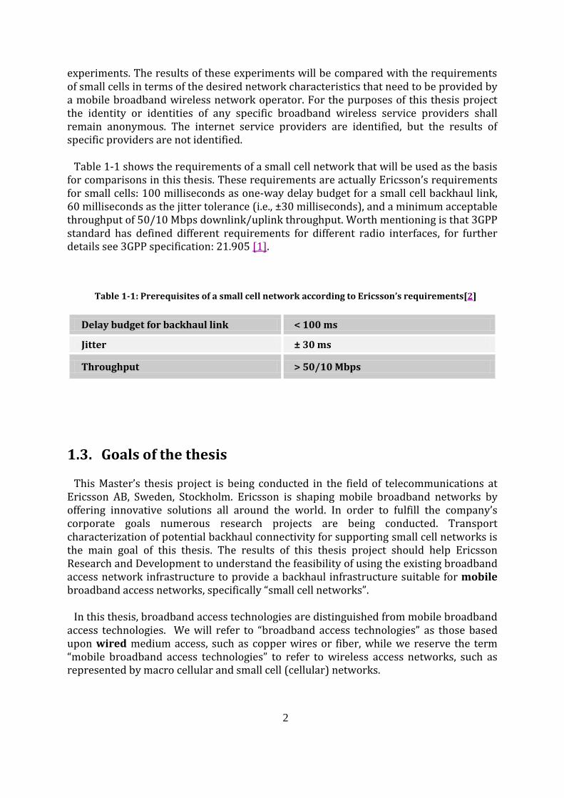
Table 1-1 shows the requirements of a small cell network that will be used as the basis for comparisons in this thesis. These requirements are actually Ericsson’s requirements for small cells: 100 milliseconds as one-way delay budget for a small cell backhaul link, 60 milliseconds as the jitter tolerance (i.e., ±30 milliseconds), and a minimum acceptable throughput of 50/10 Mbps downlink/uplink throughput. Worth mentioning is that 3GPP standard has defined different requirements for different radio interfaces, for further details see 3GPP specification: 21.905 [1].

Table 1-1: Prerequisites of a small cell network according to Ericsson’s requirements[2]

Delay budget for backhaul link < 100 ms

Jitter ± 30 ms

Throughput > 50/10 Mbps

1.3. Goals of the thesis

This Master’s thesis project is being conducted in the field of telecommunications at Ericsson AB, Sweden, Stockholm. Ericsson is shaping mobile broadband networks by offering innovative solutions all around the world. In order to fulfill the company’s corporate goals numerous research projects are being conducted. Transport characterization of potential backhaul connectivity for supporting small cell networks is the main goal of this thesis. The results of this thesis project should help Ericsson Research and Development to understand the feasibility of using the existing broadband access network infrastructure to provide a backhaul infrastructure suitable for mobile broadband access networks, specifically “small cell networks”.

In this thesis, broadband access technologies are distinguished from mobile broadband access technologies. We will refer to “broadband access technologies” as those based upon wired medium access, such as copper wires or fiber, while we reserve the term “mobile broadband access technologies” to refer to wireless access networks, such as represented by macro cellular and small cell (cellular) networks.

3

To achieve our goal the following steps were taken:

Investigating measurement tools for network characterization, Performing experiments and collecting measurements, Analyze and characterize the measured access networks, and Propose improvements to the measurement tools.

1.4. Research method

The research method used in this thesis project is based on experiments, since the existing data about the characteristics of various broadband access networks is not sufficient to compare with the requirements of small cell networks. These experiments could be performed in real networks or in simulations of such networks. The first approach is chosen here, since real networks can give more representative (of the real world) results than simulated networks in a lab environment. The experiments were performed in real networks utilizing one server equipped with a Global Positioning System (GPS) receiver, and several clients connected by different service providers and via different broadband access technologies with various uplink and downlink bandwidths. The server was under our full control, but the clients were distributed to volunteers. These volunteers were recruited from among my colleagues at Ericsson, who had cable Internet, ADSL, VDSL, or fiber broadband access network service. Communication with the clients utilized SSH connections. Tests of different aspects of the clients’ access network characteristics and the path to the server were performed.

The research approach was quantitative and measurement-oriented. The measurements were repeated several times so that an estimate of measurement repeatability would be possible. Moreover, the variance of the estimates of each of the network metrics was reduced due to these repeated measurements.

4

1.5. Structure of the thesis

The first chapter of this master’s thesis introduced the problem area and described the goals of this project. The research methodology was selected in order to fulfill the goals.

The second chapter gives a brief summary of relevant background information concerning the research area, and discusses related work in this area which has been done by others.

The third chapter describes each of the broadband access technologies (both wired and wireless) that are used in current broadband access networks.

The fourth and fifth chapters present the different measurement methods and tools, which have been used in this project, together with the test bed environment and measurement infrastructure for the experimental part of this thesis project, respectively.

The sixth chapter describes the results of the measurements and analysis of each of the case studies.

Finally, the last chapter presents the conclusion of this thesis project and discusses the future work that should be considered in a continuation of this project.

5

Chapter 2

Background

The main purpose of broadband access networks is to solve the “Last Mile” problem. The last mile refers to the final link distance from a service provider to its subscribers. This link can be provided via different types of broadband access technologies, such as digital subscriber lines (xDSL), fiber, cable-TV, and various types of wireless broadband access technologies (as shown in Figure 2-1). This connection between subscribers and the core network infrastructures of service providers is a critical issue, since the characteristics of the network as experienced by the subscribers is important (to attract and retain customers, to support various services,…)[3].

Internet Backbone

ISP Building

Radio

Base

Station

Copper lines

Fiber Lines

SubscriberCPE

Radio

Base

Station

Figure 2-1: Last Mile Connectivity

(CPE stands for Customer Premises Equipment, ISP stands for Internet Service Provider)

6

In this thesis, an active probing method is used in order to examine real networks with regard to various network characteristics. These characteristics are discussed in the next subsections.

Active probing is a method for collecting network performance measurements. This is one of the common means to evaluate a network. This method depends upon actively injecting test packets into the network. These packets are called probe packets, containing some probe data with a small amount of information such as time stamp [4]. One of the difficulties of active probing is that this additional traffic can alter the behavior of the network being studied, for example, by causing congestion (leading to packet loss) when congestion would not normally exist and increasing delay due to the added traffic load and processing of the probe packets. Additionally, unless these packets look like the normal packets being used for the service that is being considered, there is a risk that these packets are treated differently than the packets of interest somewhere along the network path. More details of these measurements and the effects of probe traffic will be discussed in next sections.

2.1. Small cell Networks

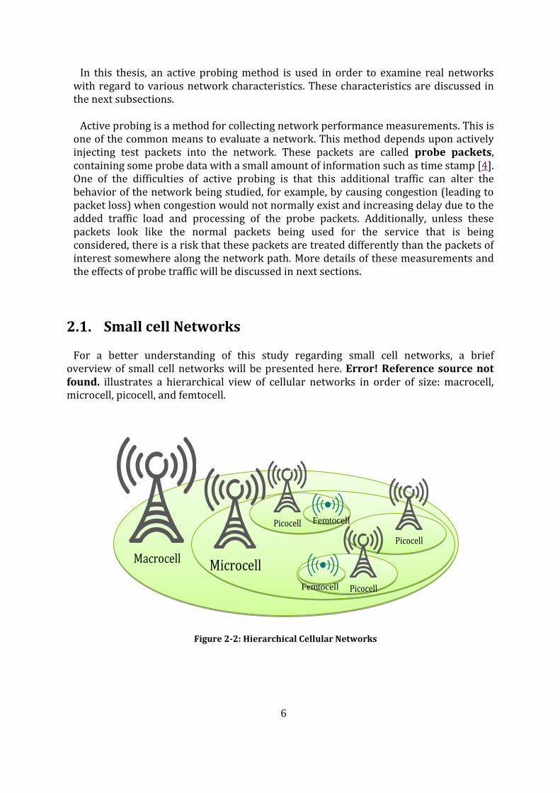
For a better understanding of this study regarding small cell networks, a brief overview of small cell networks will be presented here. Error! Reference source not found. illustrates a hierarchical view of cellular networks in order of size: macrocell, microcell, picocell, and femtocell.

Macrocell Microcell

Picocell

Picocell

Picocell

Femtocell

Femtocell

Figure 2-2: Hierarchical Cellular Networks

7

In this thesis, we will only consider small cell networks with coordinated small cells. Thus, uncoordinated networks (such as femtocells) will not be considered in this research, since they are only for private usage and they already make use of a customer’s network as their backhaul. In contrast, the other types of small cell networks have traditionally used dedicated backhaul network. Section 2.1.1 describes Wi-Fi small-cells which as femtocells will not be considered in this thesis.

2.1.1. Wi-Fi

Wi-Fi1 (based on IEEE 802.11 standard) is another type of small cell heterogeneous networks. Wi-Fi uses low power access points to create a radio access network [5]. It is worth noting that Wi-Fi and micro/picocellular networks (i.e., small cell technologies) are complementary. Wi-Fi can be combined with the Third Generation Partnership Project (3GPP) cellular network in many places (such as offices, stadiums, restaurants, etc.) to provide a seamless user experience. Hence, Wi-Fi is a solution for capacity problems in high user density or high traffic locations. In other words, Wi-Fi can fill the gaps of network coverage, where the other services of 3rd Generation mobile broadband (3G) operators is not available. Another point which should be noted is that, Wi-Fi capability is integrated in many current devices, that makes it very convenient for users.

Wi-Fi is very cost effective for new installations and upgrades, since there are already Wi-Fi networks in place for many users. Nevertheless, a remaining question is: How can we use Wi-Fi in combination with other types of small cell networks to solve capacity problems? In order to answer this question, knowledge of “Wi-Fi-offloading” is required.

Wi-Fi-offloading refers to transferring data through a Wi-Fi interface rather than via a cellular network interface. This can be done in two different ways. First, data could be transferred immediately via a Wi-Fi interface. Note that this can only be done if the device is within the coverage area of a Wi-Fi access point and the user is authorized/permitted to utilize this access point to transfer this contents. Otherwise, the user will have to transfer the content via a 3G network or some other network. This method of transfer via Wi-Fi is called “On-the-spot”. The second method is called “Delayed offloading”, in this alternative method the data transmission is done at some other point in time when the user has Wi-Fi access. (Note that it might even be done in advance of the user requesting this content if there is a means to predict that this content is likely to be requested in the future). However, the delayed offloading should be completed within a pre-defined period, and if it cannot complete the transmission by this deadline, then another type of network such as 3G will be used to complete the transfer [6].

In general, the small cell networks that we will consider can be divided into two categories: microcells and picocells. Each of these will be described in a subsection.

1 Here “Wi-Fi” as a term refers to networking equipment that meets one or more of the IEEE 802.11 standards

and that passes the interoperability test of the Wi-Fi Alliance (i.e., is Wi-Fi CERTIFIED™).

8

2.1.2. Microcell

Reducing the size of cells in cellular networks, helps improve the performance of cellular networks in certain areas. A microcell is one solution to increase capacity in areas that are dense with users. In a microcell the coverage of the cell is limited to few hundred meters and less than 2 kilometers [7].

2.1.3. Picocell

Low power base stations (often called picocells) were introduced to improve the network coverage and capacity at low cost. This type of base station is designed primarily for the indoor usage. Such low power base stations have a range of few hundred meters. These base stations are most suitable for locations with a high load traffic and slowly moving users, such as in airports, shopping malls, train-stations, libraries, offices, etc. [8] .

2.2. Networks characteristics

In order to characterize small cell networks an enumeration of the characteristics of these networks is needed. The network performance characteristics that this thesis project concerned with are:

Bandwidth and Throughput, Delay, Jitter (Delay variation), Packet Loss, and Fluctuations in these performance metrics.

The following subsections give a short description of each of these metrics.

2.2.1. Bandwidth and Throughput

Link bandwidth is the capacity of the link and is measured in units such as megabits per second (Mbps). Bandwidth refers to the volume of data which can be transferred via a link in a network between a sender and receiver in a unit period of time [9]. However, the most interesting network metric is “Available Bandwidth”. The term “available bandwidth” refers to the unused bandwidth of the link , which could be utilized without disturbing the existing traffic flows being carried via the link [10, 11]. Throughput is the actual amount of data per unit time which is successfully transferred via a communication channel from sender to receiver, and (without the use of compression) is less than the bandwidth [12]. The focus of our measurement will be on throughput,

9

since that is the real indicator of the achievable network performance. Note that in our experiments we will actually be measuring bandwidth and throughput for a network path from sender to receiver, rather than simply measuring a single link. We assume that the throughput will be characterized by the minimum throughput link (as this link will produce an upper bound on the available bandwidth). In general we expect that this link will be in the last mile, as the backbone of the network operator is assume to have sufficient aggregate capacity that our probe traffic will not experience any significant impairments in the core network. This assumption will be verified in the measurements of different networks.

2.2.2. Delay

Measurements of delay in this thesis project will be concerned with one-way delay. One-way delay is the latency from a source to a destination, i.e., the time that it takes for the first byte of a packet to be received by the receiver after being sent by the sender. Measuring one-way latency requires that the clocks at the sender and receiver be synchronized. This synchronization is typically done by using the network time protocol (NTP) [13], precision time protocol (PTP) [14], or an external time source such as a GPS receiver and the GPS system. Measuring one-way delay is described in many papers, such as [15] and the relevant IP performance metrics are described in RFC 2679 [16].

More details about the network architecture in which we conducted our measurements will be discussed later in Chapter 5.

2.2.3. Jitter (Delay Variation)

Jitter is the delay variation of packets in a stream [4]. This parameter is very critical for this project, since for some types of small cell base stations we need to provide synchronous transmission emulation over the network, hence a large variation in delay would be unacceptable [11]. For this reason, the lower the jitter, the better and more stable the emulation of a synchronous channel will be. Note that synchronous channel emulation across a packet network is often referred to as a pseudo-wire. For some further insight into pseudo wires see RFC 4447 [17].

However, we will not use pseudo-wire for small cells here. We are simply trying to determine how low jitter is in practice so that if the broadband connection were to be used for a backhaul that the phase and/or frequency synchronization would be as accurate as possible, as well as to enable soft-handover [18] for 3G networks.

10

2.2.4. Packet Loss

When a packet, which has been sent from sender, does not reach to receiver, a packet loss has occurred. This loss is considered a one-way packet loss, since the path that a packet traverses from sender to receiver may not be exactly the same path that a packet would use from this receiver back to the original sender. In some cases, corrupted or faulty packets are also be considered to be lost packets [19] .

Packet loss is not be one of the metrics we focus on in this thesis, as the actual packet loss observed in our measurements should be sufficiently low as to be acceptable. This means that the packet loss rate should be less than 1%, otherwise we will not consider our measurements to be valid.

2.2.5. Fluctuation

Fluctuation in bandwidth will lead to a variation in the throughput of a link. When bandwidth increases and decreases continuously, there will be a corresponding variation in throughput. However, some protocols react adversely to decreases in throughput (as they may interpret this as congestion), hence in order to provide good quality of service (QoS), (rapid) fluctuations in bandwidth should be minimized.

In order to measure each of these criteria, different measurement tools and protocols will be used. These measurement tools and protocols will be discussed in Chapter 2.

2.3. Related work

Similar work has been done, such as the study performed in 2007 by M. Dischinger, et al. [20] of residential broadband networks which assessed several characteristics of the networks in Europe and North America, in terms of round trip time (RTT), jitter, packet loss, throughput, etc. Their study focused on DSL and cable networks and pointed out the differences in the behavior of these residential networks. These types of networks are typically the most critical part of the access network, i.e., “Last Mile”. In this thesis project, not only cable and DSL networks are considered, but also other types of broadband access networks, such as fiber. In Sweden, a number of providers provide various data rate fiber to the home or fiber to the curb based solutions. The measurements in this thesis cover quite a wide range of different types of last mile access networks and the measurements have been done in real networks in order to give a better view of the situation today. In this sense this thesis project gives a more comprehensive picture of broadband access network characteristics today.

Another similar work is the research which done by N. Hu and P. Steenkiste [21], where they evaluated probing methods for measuring available bandwidth. They used both simulations and measurements of different kinds of links and considered different

11

factors, such as competing traffic on a link, packet size, and probe train size1. These parameters helped them find the factors that could affect the accuracy of their measurements. A conclusion of their work was that the main factor that could make the measurement of the available bandwidth more accurate is the gap between packet trains. They also assessed networks in terms of traffic load: congested lines and low traffic load lines2, to show the impact on accuracy of different tools, although the accuracy of results overall was not really affected. This thesis focuses on different kinds of broadband access networks regardless of their traffic loads, since they all are real networks and can have different loads at different times of the day. Moreover, other characteristics of these networks (such as jitter, delay, and packet loss) have been considered and will be discussed later in this thesis.

Regarding different technologies, there are also several projects, which have characterizes the different types of networks. We will refer to the projects when we discuss the details of this thesis project.

1 A probe train is a sequence of probe packets. We can exploit measurements of the intervals between packets

to examine queuing delays and jitter.

2 A traffic line is considered as congested, when the delay increases and the network starts to drop the packets.

This means that if there is no dropped packets and/or a large jump in delay, that line is considered to have a low

traffic load.

13

Chapter 3

Broadband Access Technologies

Broadband access technologies refer to access network technologies which provide high link data rates. These technologies are categorized in two groups [11]:

1. Wired broadband access technologies, which provide access through physical links, and

2. Wireless broadband access technologies, which provide access via radio, optical, or other wireless links.

The most common broadband access technologies, considering both wired and wireless categories are:

Digital Subscriber Line (DSL), in its variants: ADSL, ADSL2+, and very high speed DSL2 (VDSL2);

Point to Point Ethernet over Fiber, Fiber To The X (FTTX)- where X can be Home, Curb, …, Ethernet Passive Optical

Network (EPON), and Gigabit Passive Optical Network (GPON); Cable-TV networks, using a cable modem to realize broadband access over a

cable-TV network, typically using the Data Over Cable Service Interface Specifications (DOCSIS) standard [22]; and

3G or 4th Generation mobile (cellular) broadband(4G), IEEE 802.16 as realized by Worldwide Interoperability for Microwave Access (WiMax), IEEE 802.11 as realized by Wi-Fi products, and satellite links,

14

3.1. Digital subscriber line technology

DSL is an access technology, which can provide several different access services through twisted pairs of telephone lines at the same time. DSL technology is widely used to provide data access links to users over the existing copper wire infrastructure (primarily that installed earlier for analog telephony). A variety of DSL technology is indicated by the generic name xDSL, which includes ADSL, ADSL2, ADSL2+,… [23] .

DSL modem users utilize an end-to-end dedicated connection to a Digital Subscriber Line Access Multiplexer (DSLAM), where the data and telephone signals are separated [24]. Note that the copper cabling over which these signals are carried is typically, in large bundles, hence there is cross talk between the different wires. The DSL modem and DSLAM carry out measurements and adapt based upon the results of these measurements. Hence the characteristics of a given modem’s communication with a DSLAM can change because of what other users do (for example, their current traffic or absence of traffic).

Central Office

Subscriber

DSLAMDSLAMDSLAM

SwitchSwitchSwitch

DSL

Modem

PSTNPSTN

InternetInternet

Phone

Figure 3-1: DSL Network Setup

ADSL is asymmetric type of DSL. This means the data rates for downloading and uploading are different. ADSL provides downloading at up to 7 Mbit/s, while the uploading data rate is about 256 Kbit/s [25] .

ADSL2, is an improved version of ADSL which provides double the peak data rates for both downstream and upstream [26]. The newest and extended version of ADSL2 is ADSL2+. ADSL2+ was designed to provide three times faster download data rate and of course, an increased peak upload data rate as well. Another service, which is supported by ADSL and ADSL2+, is QoS, which is important in some specific networks [27].

Very high data-rate DSL2 (VDSL2) is another broadband access technology. The goal of VDSL2 broadband access networks is to provide sufficiently high data rates for advanced voice and video services, such as video conferences or voice over IP (VoIP). The peak data rate provided by VDSL(2 is up to 100 Mbps for both uplink and downlink [28]. However, the tariffs for using this access technology are usually very high. It should be noted here that this information concerns the current situation, and might be changed in the near or far future. Based upon the tariffs of one of the biggest ISPs in

15

Sweden, “Telia” [29], the price of lower bandwidth with VDSL is much higher than the price of higher bandwidth with fiber broadband access network. However, the price of low bandwidths for both VDSL(2 and fiber is almost the same for this same ISP, (but only if the fiber infrastructure is already available, and there is no need to burry new fibers). Moreover, the difference in price between high bandwidths for VDSL(2 and fiber indicates that in these cases, ISPs are trying to encourage people to move to fiber, instead of utilizing VDSL(2, as it eliminates the need for them to operate VDSL(2 DSLAM.

3.2. FTTX, EPON, and GPON

Using fiber as broadband access technology is very popular in many countries, such as Sweden. Reasonable subscription rates for very high uplink and downlink speeds have increased the market penetration of this technology. In this section, several different approaches to using fiber as a broadband access network are introduced. Several of these alternatives are shown in Error! Reference source not found..

The technology which is primarily used in Sweden is FTTX (point-to-point Ethernet) rather than EPON and GPON (multi point for multi subscribers). Both EPON and GPON technologies use shared resources in both downstream and upstream directions.

3.2.1. Fiber to the x (FTTX)

Different types of fiber-based broadband access technologies, such as fiber to the home (FTTH), fiber to the building (FTTB), fiber to the curb (FTTC), and fiber to the node (FTTN) are all collectively referred to as FTTX. Using fiber as the transmission media provides a large amount of bandwidth over longer distances to subscribers. Peak data rates can exceed a gigabit per second data rate, while the subscription price is affordable. For some further details on pricing, see the recent thesis by Ziyi Xiong [30].

Fiber-To-The-Home (FTTH), is a fiber-based broadband access technology which provides home users with a fiber interface to each home [31]. This method supplies 155 Mb/s to 2.5 Gb/s speed downstream, and 155 Mb/s to 1 Gb/s upstream [32].

Fiber-To-The-Building (FTTB) is similar to FTTH, with the difference that the fiber interface is generally placed in the basement of the building. From this point access is generally distributed to users via other broadband access technology such as VDSL(2) or Ethernet [33]. Alternatively, some buildings connect each apartment in a building with an access fiber to the basement with optical interconnects, hence realizing a FTTH infrastructure.

Fiber-To-The-Curb (FTTC) is another fiber-based broadband access technology. This alternative brings the fiber interface to a cabinet in the street outside of a group of homes. The connectivity continues to subscribers using copper pairs through VDSL(2) or

16

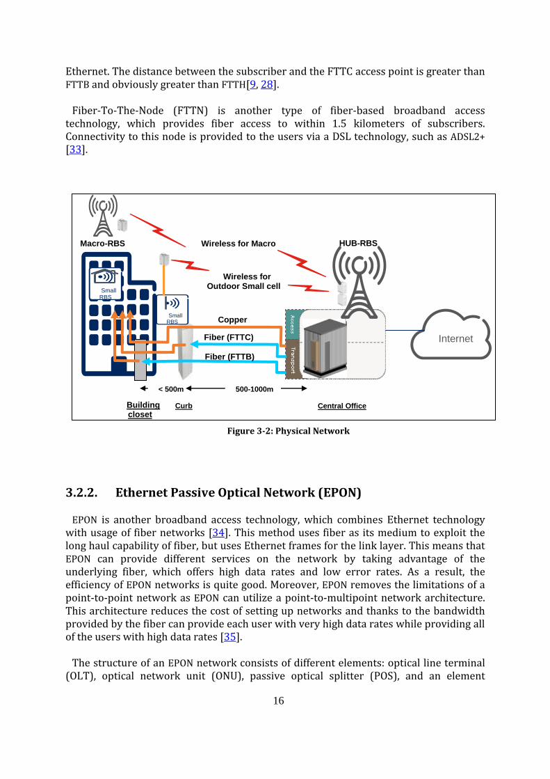
Ethernet. The distance between the subscriber and the FTTC access point is greater than FTTB and obviously greater than FTTH[9, 28].

Fiber-To-The-Node (FTTN) is another type of fiber-based broadband access technology, which provides fiber access to within 1.5 kilometers of subscribers. Connectivity to this node is provided to the users via a DSL technology, such as ADSL2+ [33].

3.2.2. Ethernet Passive Optical Network (EPON)

EPON is another broadband access technology, which combines Ethernet technology with usage of fiber networks [34]. This method uses fiber as its medium to exploit the long haul capability of fiber, but uses Ethernet frames for the link layer. This means that EPON can provide different services on the network by taking advantage of the underlying fiber, which offers high data rates and low error rates. As a result, the efficiency of EPON networks is quite good. Moreover, EPON removes the limitations of a point-to-point network as EPON can utilize a point-to-multipoint network architecture. This architecture reduces the cost of setting up networks and thanks to the bandwidth provided by the fiber can provide each user with very high data rates while providing all of the users with high data rates [35].

The structure of an EPON network consists of different elements: optical line terminal (OLT), optical network unit (ONU), passive optical splitter (POS), and an element

< 500m

Copper

Fiber (FTTC)

Fiber (FTTB)

Wireless for Macro

Wireless for Outdoor Small cell

500-1000m

Central Office Curb

HUB-RBS

Small RBS

Small RBS

Internet

Macro-RBS

Building closet

Figure 3-2: Physical Network

17

management system (EMS). An OLT is a terminal that resides in a central office of the service provider and is responsible for connecting the optical access network to the service provider’s backbone network. The ONU is the final part of the EPON network, as it connects the access network to the end user, hence it should be located close to the subscriber. A POS provides a connection between the OLT and ONU. This element acts as a splitter in the downstream direction and behaves like a combiner in the upstream direction. Finally, the EMS enables the service provider to manage, maintain, configure, and control the different elements of the EPON [29, 31].

EPON utilizes Time Division Multiplexing (TDM) for the upstream links, in order to avoid any collisions between the different users’ channels. This means that access to the upstream link is shared based upon time division multiplexing of each of the ONUs [37].

3.2.3. Gigabit Passive Optical Network (GPON)

GPON is another type of broadband access technology. It is mostly used to provide data rates of at one gigabit per second or more. The GPON standard is based on the ITU-T G.984 recommendations [38]. An advantage of GPON over EPON, is that GPON provides much higher bandwidth for both uplink and downlink directions. Moreover, GPON uses wavelength division multiplexing (WDM). This means that both uplink and downlink signals are multiplexed onto the fiber using different wavelengths, so traffic can be sent in both direction by multiple users on a single optical fiber [39].

3.3. Broadband on Cable-TV Networks

Cable modem access technology was an earlier alternative to fiber-based access. The purpose of a cable modem was to provide Internet connectivity over a cable-TV network. Cable-TV networks use shared resources in both down and upstream directions. The TV channels and Internet packets shared the cable by having the cable modems use different frequencies for their up and down links from the frequencies used by the TV channels (which were quite often asymmetrically divided – i.e., with many more TV channels in the downlink direction that in the uplink direction) [31].

In relation with cable-TV networks, P. Jacquet, [40] explicitly studied this type of network in terms of bandwidth management with the focus on upstream channels.

3.4. Wireless broadband

Wireless broadband access technologies emerged to provide broadband access for mobile users, i.e., to provide mobile users with a high peak data rate [41]. However, providing mobility is different from simply providing wireless access. Mobility is supported when a user moves from one cell to another one while continuing to transfer data, voice, video, or any other types of data, without any interruptions in the

18

communication or session. In contrast, wireless access simply provides access via a wireless access link [42].

Wireless technologies (except satellites), use shared resources in both downlink and uplink directions.

3.4.1. WiMax

WiMax is a wireless broadband access networks that utilizes the IEEE 802.16 standard. This standard is mostly concerned with the media access control (MAC) layer and the physical layer. WiMax is the industrial realization of this standard. The goal of WiMax is to connect enterprise or individuals subscribers to the Internet with very high capacity and performance [43].

3.4.2. Wi-Fi

Wi-Fi is a very common wireless access technology, based on the IEEE 802.11 standard. Wi-Fi is the trade name for IEEE 802.11 products that are certified by an industrial alliance. The goal of this alliance is to promote interoperable WLAN technology. Wi-Fi is used for both indoor and outdoor networks and has a maximum range of 50 to 100 meters with omni-directional antennas [40, 43]. Much longer links can be supported with directional antennas.

3.4.3. 3G

The third generation (3G) of wide area cellular technology is a wireless broadband access technology, provided by mobile communication service providers. The main advantage of this technology is that it provides users with continuous Internet connection in the union of the coverage areas of the service provider’s mobile base stations. Handovers between cells are managed by the network (perhaps in conjunction with the terminals). The base stations typically can support a moving user at a range of up to several kilometers [45]. 3G technology is now a very common broadband mobile access technology and is supported by most of the mobile operators around the world.

3.4.4. 4G (LTE)

The latest generation of wide area cellular access technology is called 4G. The 3GPP has developed a series of standards that have led to Long Term Evolution (LTE) as another mobile broadband access technology. LTE offers a high capacity mobile broadband network and provides subscribers with high data rates and a very low delay over LTE links [46].

19

3.4.5. Satellite links

Satellites are another mobile-broadband access technology. Satellites are widely used to provide a broadband access network where there is no possibility to have access via traditional access networks [47]. The upstream link capacity of satellites is typically 1 Mbps, but the downstream data rates could be as much as 1 Gbps [44].

3.5. Summary

Choosing a suitable broadband access technology depends on many different criteria, such as:

Existing infrastructure, Geographic location, Number of subscribers, Type of the service to be provided by the network, and Capital and operating expenses. [48]

21

Chapter 4

Measurement Tools and Methods

This chapter will review a number of different measurement tools utilizing active and passive methods and discusses the attributes of each of these methods.

4.1. Active versus Passive measurements

An active measurement method uses one or more probe packets by injecting the packets into networks in order to measure some characteristic(s) of the network. These probe packets do not necessarily contain any data and they are generally sent at a very low average rate, as a result, they will generally not cause excessive traffic loads in the network. Moreover, using probe packets avoids the need to have access to specific parts of the network (such as routers) in order to collect measurement data. In contrast, passive measurement tools collect data through counters in the network which have been defined beforehand in order to observe specific characteristics of the network [49]. The advantage of passive tools is that no additional traffic is needed (other than to transfer the collected data). Their disadvantage is that you need to have permission to access these counters.

No passive measurement tools will be used during this research, since access to the counters required for collecting data is generally limited to the network operations portion of the network operator themselves. The focus will instead be on the uses of active measurement tools. We will examine some tools from this category in the 4.2 section.

22

4.2. Active measurement tools

This section describes a variety of active measurement tools. Some of these tools will be used for collecting data concerning the networks that we have examined in this thesis project.

4.2.1. IPERF (Internet Performance Working Group)

IPERF is a tool for measuring the performance of a network. It measures the end-to-end available bandwidth of a network, with the ability to set the time of transmission and the number of packets to be transferred via a Transmission Control Protocol (TCP) stream [50] (see Figure 4-1). By available bandwidth, we are referring as noted earlier to the unused capacity of the path over which we are making our measurements. The two hosts send data to each other during a specific period. The available bandwidth can be highly time-dependent and depends on whether the network path is occupied by traffic or not - as the available bandwidth can be quite different in these two cases [7, 45].

IPERF can also utilize User Datagram Protocol (UDP) mode as well. IPERF works in client-server mode [52], this means that in the network that we wish to measure there should be a client which can act as a reflector for traffic generated by the server [50].

The advantage of this active measurement tool is that IPERF can utilize several TCP streams at the same time and as a result gives a better view of the available bandwidth. This property makes it a very common and popular tool for measuring available bandwidth in networks [51].

The default setting of IPERF in order to measure the performance of a link is a transmission time of 10 seconds with the TCP window size of 16KB. These values can be tuned for a specific measurement. During this transmission period, IPERF sends out probe packets to use up the available bandwidth of the link and in this way estimate the capacity of the network [53]. (It should be noted that IPERF loads the network with as much traffic as possible).

Iperf

Server

Iperf Client

Network

Available

Bandwidth

Figure 4-1: IPERF measurement network setup

23

4.2.2. Network Time Protocol (NTP)

NTP is the most common protocol for synchronization of clocks over Internet. This protocol exists in different revisions, and the version which was used in this thesis project is NTP version 4 (NTPv4). This version has more functionalities than the previous version (NTPv3). The most important feature is the accuracy of timestamps, which has been improved and is less than one nanosecond [13].

The actual accuracy of NTP depends on the network delay, jitter, and delay symmetry. In this thesis, NTP was used to synchronize the client’s clock to our server’s clock. The server is in turned synchronized with coordinated universal time (UTC) by using a GPS receiver.

4.2.3. One-Way Active Measurement Protocol (OWAMP)

As an active measurement protocols, OWAMP [54] provides the ability to measure the delay in one-way direction over the links between two nodes in a network [55]. In order to achieve this goal, OWAMP needs to have highly precise time stamps in order to accurately estimate the delay of the link. GPS receivers are usually used to guarantee the accuracy and synchronization of the sender and receiver clocks for making such a measurement.

OWAMP consists of two sub protocols called OWAMP-Control and OWAMP-Test. OWAMP-Control is responsible for starting and stopping sessions between two nodes and then collecting results of the measurements of the one-way delay between these two nodes. OWAMP-Test is responsible for sending the packets which are sent during such a measurement campaign [56].

The communication between two nodes utilizes a TCP connection on a specific TCP port. This TCP connection will remain open during the whole testing session. In fact, TCP is used for controlling traffic and for making the collection of measured data possible, while UDP protocol is used for sending and carrying the measured data. This means that UDP datagrams are sent over the TCP connection. The test traffic supports three types of UDP datagrams: authenticated, unauthenticated, and encrypted. Each of these three modes should be specified beforehand by the sender node [54].

While the receiver listens to the TCP port, the receiver is also listening to a specific UDP port for test traffic. During a test UDP datagrams are transmitted between the two endpoints. The time stamps of the sender and receiver are used by algorithms to estimate the one-way delay.

24

4.2.4. BART including TWAMP

The two-way active measurement protocol (TWAMP) is an enhanced protocol that provides round-trip delay measurements between two hosts. TWAMP has also two sub protocols (similar to OWAMP), which are called: TWAMP-Control and TWAMP-Test. Communication between client and server is initiated by establishing a TCP connection from the client to the server’s TCP port 862. In TWAMP both sides send and receive UDP datagrams to make the two-way delay measurement. More details of the TWAMP protocol can be found in RFC 5357 [57].

Bandwidth Available in Real Time (BART) is a measurement tool, which utilizes the TWAMP protocol for bidirectional measurements. BART sends a train of packets rather than a single packet between the two endpoints, within pre-defined intervals. BART uses active probing in order to measure the available bandwidth of a link. BART applies Kalman filtering as part of the BART analysis of results. The Kalman filtering is used when analyzing the probe packets in order to estimate the real-time bandwidth of an end-to-end path (which implicitly makes the assumption that all packets are sent over the same path during a testing session). The continuous estimation of available bandwidth of a link improves the analysis of the next probe packets [12].

Estimating the available bandwidth of a link helps in several different ways, such as developing adaptive applications which matching their transmission rate to the capacity of the link or performing traffic management in order to prevent congestion [58].

4.2.5. TPTEST

TPTEST is an open-source tool, written in the C++ programming language, which was developed by the Swedish Post and Telecom Authority (PTS). This tool is available for several different operating systems. The purpose of developing this tool was to allow Swedish customers to evaluate the quality and performance of their Internet connectivity, from a throughput perspective. It was thought that this would help users to choose the best Internet service provider [59].

TPTEST has a list of servers, which are currently all located in Sweden, and in order to measure the throughput of a line, it uses one of these servers to communicate with a user’s machine to collect information regarding the performance of the user’s Internet connectivity. The main output of this tests includes downlink and uplink throughput for TCP and UDP, RTT, and packet loss [59, 60].

Since TPTEST is designed so that any user even one without any knowledge of networks should be able to use it to evaluate their broadband connectivity, the program offers two modes: basic and advanced. A description based upon [59] of both modes is given in the following subsections.

25

4.2.5.1. Basic mode

Basic mode that is designed to provide very basic information, but also offers two options to the user. The first option is the Standard Test in which the server that a user does the measurement against is always located in Stockholm with all the default and the recommended configurations are supplied by the server. The second option is a Selective Test which gives the user an opportunity to choose the type of measurement (downlink, uplink, ...) and to select the server which this user wants to measure their broadband connectivity with.

4.2.5.2. Advanced mode

Advanced mode is obviously for advanced users who have greater measurement knowledge (or desires), and who wish to customize their measurement results. In this mode, users get the chance to not only select the server they wish to utilize, but also to select the port number which they prefer to use for the transmission of data between their machine and server.

This mode also provides measurements for both TCP and UDP. In addition, users can customize the transmission time between 1 to 30 seconds and specify the amount of data they wish to transfer during that specific period.

4.3. Passive measurement tools1

Unlike active measurement methods, in passive measurement no probe packets are injected to the network, but rather real network traffic statistics is collected and visualized using different tools [61]. Multi-Router Traffic Grapher (MRTG) is a passive measurement tool which is widely used to estimate the available bandwidth of the link. It collects information about the amount of data traffic forwarded through a router.

MRTG is a simple network management protocol (SNMP)-based tool. It has been built based on the SNMP specifications for monitoring networks. The SNMP protocol itself is a passive method for collecting performance data of a specific device. Using SNMP, MRTG can keep track of the traffic over various links in the network by calculating the data traffic rates over different intervals of time, by collecting information from counters in the router for each of the router’s different interfaces. Based upon this data, MRTG calculates the difference between the counter’s earlier value and its present value, and divide this by the interval in time between the two instances of data collection to compute a traffic rate [61]. MRTG collects data from counters on router interfaces [56].

1 Note that no passive measurement tool is used in this thesis, and MRTG is just an example of that category.

26

4.4. Summary

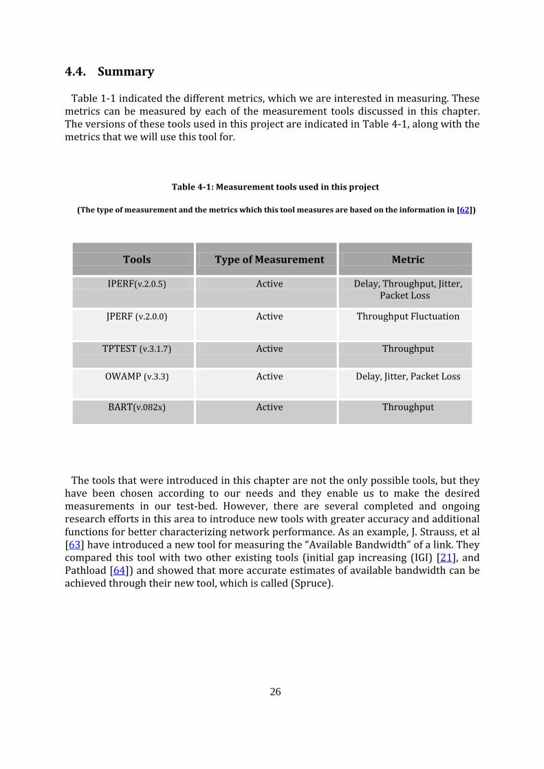
Table 1-1 indicated the different metrics, which we are interested in measuring. These metrics can be measured by each of the measurement tools discussed in this chapter. The versions of these tools used in this project are indicated in Table 4-1, along with the metrics that we will use this tool for.

Table 4-1: Measurement tools used in this project

(The type of measurement and the metrics which this tool measures are based on the information in [62])

The tools that were introduced in this chapter are not the only possible tools, but they have been chosen according to our needs and they enable us to make the desired measurements in our test-bed. However, there are several completed and ongoing research efforts in this area to introduce new tools with greater accuracy and additional functions for better characterizing network performance. As an example, J. Strauss, et al [63] have introduced a new tool for measuring the “Available Bandwidth” of a link. They compared this tool with two other existing tools (initial gap increasing (IGI) [21], and Pathload [64]) and showed that more accurate estimates of available bandwidth can be achieved through their new tool, which is called (Spruce).

Tools Type of Measurement Metric

IPERF(v.2.0.5) Active Delay, Throughput, Jitter, Packet Loss

JPERF (v.2.0.0) Active Throughput Fluctuation

TPTEST (v.3.1.7) Active Throughput

OWAMP (v.3.3) Active Delay, Jitter, Packet Loss

BART(v.082x) Active Throughput

27

Chapter 5

Measurement Infrastructure and Test bed

This chapter will discuss the infrastructure and the environment in which we performed our measurements. These measurements have been concluded for a quite long time (from August 2012 until May 2013), in order to confirm the validity and repeatability of the achieved results.

5.1. Environment setup

The following subsections describe how the measurement test bed was configured. Figure 5-1 shows an overview of this test bed.

5.1.1. Hardware (Clients, Server, GPS)

The set of hardware that has been used to setup the measurement environment includes a number of reflectors (client machines) and a server machine to remotely control the clients. All of these reflectors were distributed to 13 randomly selected coworkers who had different Internet service providers (ISP), different bandwidths (according to their subscriptions), and different types of broadband access networks (in the measurements described in this thesis, these access networks were: Fiber, ADSL, VDSL(2), and Cable-TV).

All of the providers and networks that have been utilized in this project were located in Sweden. The specific clients were selected based on the type of their broadband access technology and the bandwidth associated with their subscription with their ISPs. The clients were purposely distributed to collect data for different types of access networks. Table 5-1 indicates the specifications of the clients involved in our measurements.

28

Table 5-1: Specifications of users involved in measurements

ISP Type of broadband access technology

Bandwidth (DL/UL) Mbps

Client1 OwnIT Fiber 100/100

Client2 Telia Fiber 100/10

Client3 BredbandsBolaget Fiber 100/10

Client4 BredbandsBolaget Fiber 100/10

Client5 Tele2 Fiber 100/100

Client6 AllTele Fiber 100/100

Client7 Comhem Cable-TV 100/10

Client8 Comhem Cable-TV 200/10

Client9 BredbandsBolaget ADSL2+ 13/1

Client10 Telia ADSL 7/1

Client11 BredbandsBolaget VDSL2 40/10

Client12 Telia VDSL2 23/2

Client13 Telia VDSL2 30/12

In addition to the server and clients machines, a GPS receiver was connected to the server in order to provide the server with accurate time stamps and clock synchronization with coordinated universal time (UTC). The server was synchronized using the GPS receiver and then all the clients were synchronized with this server using NTP.

Communication between the server and the clients was done remotely through SSH connections. In addition, all of the tests ran automatically every 7 hours, to get clear picture of network characteristics at different times of a day. Note that an interval of 7 hours was used rather than 8 hours, so that the machines will over the course of a week sample at different hours of the day.

29

Internet

Server

GPS

Clients

Figure 5-1: Network of our measurement test bed

The complete overview of the network map set up in for the measurements of this thesis project is shown in Figure 5-2. As shown in network map, the ISPs, which were involved in these measurements, were AllTele, Telia, Tele2, Comhem, Telenor, BredbandsBolaget, and OwnIT.

Using the “trace route” tool, it was possible to collect information about the whole path from server to each of the clients. Although it was not possible to get the exact number of routers in between (because of some of the ISPs’ limitations), with the help of the logs from OWAMP, the exact number of hops could be retrieved. Most of the clients were passing through a “peering point”, which is shown in the picture, while some of them had a direct connection through a number of routers with the server.

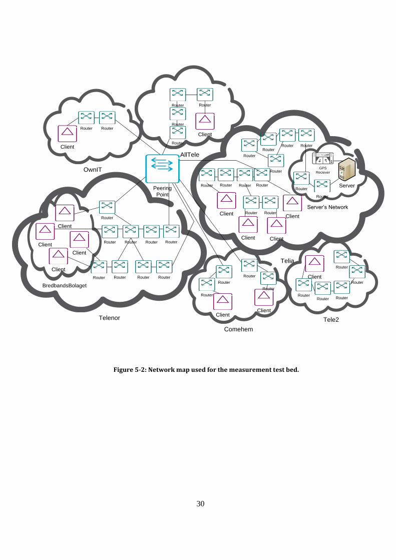
30

Figure 5-2: Network map used for the measurement test bed.

OwnIT

AllTele

Telia

Telenor Tele2

Comehem

Server’s Network

BredbandsBolaget

GPS

Reciever

Server

Client

Router

Router

RouterRouter

Router

Router

Router

Client

Client

Client

Client

Client

Client

Router

RouterRouterRouterRouter

Router

Router

Router Router Router

Client

Client

Client

Client

Client

Router

Router

Router

Router

Router

Router

Router

RouterRouter

Router

Router Router Router

Router

RouterRouter

Router

Router Router

RouterPeering

Point

Client

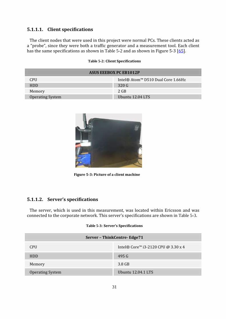
31

5.1.1.1. Client specifications

The client nodes that were used in this project were normal PCs. These clients acted as a “probe”, since they were both a traffic generator and a measurement tool. Each client has the same specifications as shown in Table 5-2 and as shown in Figure 5-3 [65].

Table 5-2: Client Specifications

ASUS EEEBOX PC EB1012P

CPU Intel® Atom™ D510 Dual Core 1.66Hz

HDD 320 G

Memory 2 GB

Operating System Ubuntu 12.04 LTS

5.1.1.2. Server’s specifications

The server, which is used in this measurement, was located within Ericsson and was connected to the corporate network. This server’s specifications are shown in Table 5-3.

Table 5-3: Server’s Specifications

Server – ThinkCentre- Edge71

CPU Intel® Core™ i3-2120 CPU @ 3.30 x 4

HDD 495 G

Memory 3.8 GB

Operating System Ubuntu 12.04.1 LTS

Figure 5-3: Picture of a client machine

32

5.1.1.3. GPS receiver

The purpose of using a GPS receiver in this research was to get accurate time-stamps by having the server synchronized with the atomic clocks in the GPS satellites. Because of the long period over which the measurements were made, it was very important to have a clock that could be stable, reliable, and accurate over this long time period. It should be noted that in order to get the clock synchronized, having at least four satellites was necessary. The GPS receiver, which was used has the specifications shown in Table

5-4.

Table 5-4: GPS Specifications

GPS Receiver - Sure Electronics GP-GS010

Time Accuracy 20 ns with 4 satellites

Protocol Message NMEA & 1 PPS output

Antenna Type Active patch antenna

Figure 5-4 illustrates the relationship between the applications running on the server, the clients, and the connection to the GPS receiver.

GPS

Receiver

1PPS + NMEAgpsd

ntpd

1PPS

Oscilloscope

1PPS

Figure 5-4: Applications running on the server and the connection to the GPS receiver used in our measurements.

33

As shown in Figure 5-4, the GPS device outputs a one pulse per second (PPS) signal, together with a text string, encoded in National Marine Electronics Association (NMEA) format, giving the actual date and time at the rising edge of the one PPS signal. The “gpsd” application, is a daemon running in the background on the server. This application receives signals from the GPS receiver reads the NMEA string via a serial port, decodes the string to extract the date and time (as well as the one PPS signal), and sends the information to the “ntpd” application.

To measure the accuracy, a software driver takes the time from the “ntpd” and emits a one PPS signal via the parallel port of the server. This 1 PPS signal can be compared with the one PPS signal from the server with the one PPS signal from the GPS using Tektronix- TBS1042 oscilloscope. This measurement which was done for 24 hours, and was controlled every 4 hours during daytime, showed a quite stable results.

The measured accuracy of GPSD with one PPS and NMEA input to NTPv4 was compared with the external GPS’s receiver’s 1PPS output showed a difference of around 40 microseconds. This difference is the error between reported measurement by OWAMP and real-time. In other words, the error of reported time stamps is 40 microseconds, which indicates the difference of the clocks.

Figure 5-5 illustrates the situation for a typical client that will be used to make measurements using a clock synchronized to the date and time information of the server as sent via the network to the client using the NTP protocol.

To compare the synchronization between the server and the client, a second GPS receiver is used at the client with a PPS output (this is done by using a USB to parallel adaptor), and this output is compared with the time due to the client’s synchronization with the server using NTP. The test setup in this case is shown in Figure 5-5. Measurement results showed around 130 microseconds time difference between the two PPS signals. However, considering the local difference between the GPS PPS and the server’s PPS as measured at the server was around 40 microseconds, a conclusion is that the actual time difference between the server’s time and the client’s time is 130 – 40 = 90 microseconds. We also made a measurement in a controlled network where client and server were both located on the same network, as described in section 5.3.2. In that controlled network we got 114 and 122 microseconds one-way delay for downstream and upstream respectively. As a result, the internal processing delay is around 74, and 82 microseconds for downlink and uplink directions which is the difference in time for processing of the PPS signals for the server and for the client. This difference is quite small and acceptable.

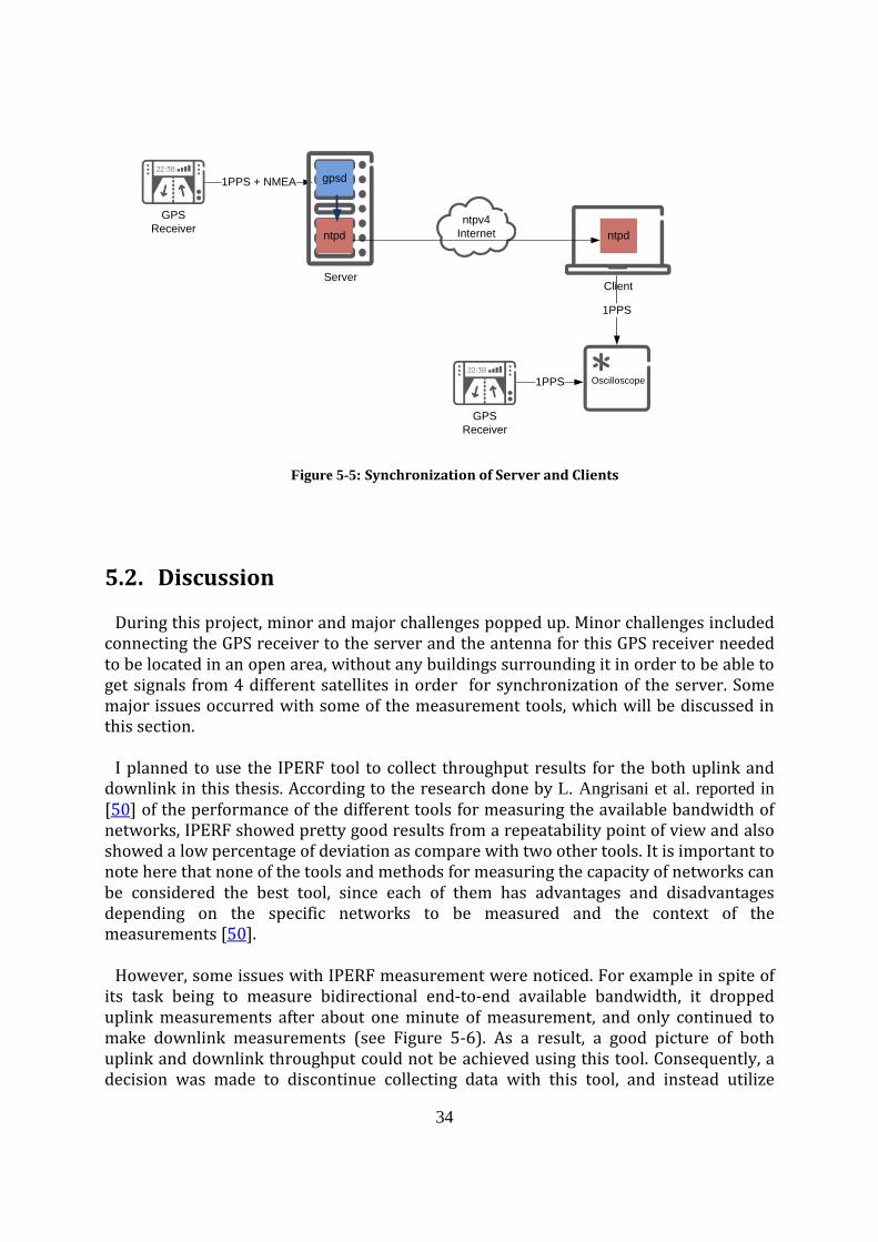
34

5.2. Discussion

During this project, minor and major challenges popped up. Minor challenges included connecting the GPS receiver to the server and the antenna for this GPS receiver needed to be located in an open area, without any buildings surrounding it in order to be able to get signals from 4 different satellites in order for synchronization of the server. Some major issues occurred with some of the measurement tools, which will be discussed in this section.

I planned to use the IPERF tool to collect throughput results for the both uplink and downlink in this thesis. According to the research done by L. Angrisani et al. reported in [50] of the performance of the different tools for measuring the available bandwidth of networks, IPERF showed pretty good results from a repeatability point of view and also showed a low percentage of deviation as compare with two other tools. It is important to note here that none of the tools and methods for measuring the capacity of networks can be considered the best tool, since each of them has advantages and disadvantages depending on the specific networks to be measured and the context of the measurements [50].

However, some issues with IPERF measurement were noticed. For example in spite of its task being to measure bidirectional end-to-end available bandwidth, it dropped uplink measurements after about one minute of measurement, and only continued to make downlink measurements (see Figure 5-6). As a result, a good picture of both uplink and downlink throughput could not be achieved using this tool. Consequently, a decision was made to discontinue collecting data with this tool, and instead utilize

GPS

Receiver

1PPS + NMEA

Client

ntpd

ntpv4

Internet

Server

gpsd

ntpd

Oscilloscope

1PPS

GPS

Receiver

1PPS

Figure 5-5: Synchronization of Server and Clients

35

TPTest (which is in principal the same as IPERF as it offers the same functionality and measures both uplink and downlink throughput).

In association with IPERF, we utilized JPERF as well. JPERF is a graphical version of IPERF that is written in the Java programming language, and gives the ability to visualize fluctuations in throughput. The JPERF graphical user interface (GUI) is shown in Figure 5-7.

Figure 5-6: IPERF Problem

(Measurement continues for only one direction after about 84 seconds)

36

Figure 5-7: JPERF Graphical User Interface

Moreover, JPERF provides different modes for measurement. In “Dual mode”, both downlink and uplink measurement can be seen at the same time. The interesting point here was that the problem we faced with IPERF tool that uplink direction was lost after about 84 seconds could not be seen here. Figure 5-8 illustrates this fact. As it is shown, after 84 seconds both uplink and downlink measurements continued until the end of this measurement period for the duration of 30 minutes. (Note that this measurement is done for only one client for a long duration, and the validity of this has not been tested for all the other users.)

37

Alternatively, one can use multiple parallel streams to see the competing streams, which shows both fluctuation and competition of streams to get their desired bandwidth. Figure 5-9 is an example of two parallel streams.

Figure 5-8: JPERF logs for two parallel streams

(Both uplink and downlink measurements continued until end)

38

When using OWAMP to calculate delay, jitter, and packet loss, a problem occurred with those clients, which were located behind a network address translation (NAT) device. When there is a NAT device in between the client and the server, the client does not have access to the external IP address, but rather the server sees only the NAT device’s IP address. As a result, this prevented us from being able to measure the one-way delay. When the OWAMP client is located behind a NAT, the server cannot reach the client, since the OWAMP client sends packets with an invalid IP address in its messages. The results is that the IP address of the client will not be the same as the IP address which the NAT device places in the source IP address field of the packets that it forwards to the server. Hence, measuring the one-way delay for those clients which were behind a NAT failed.

For a better understanding, it should be noted that the TCP session could still be established between OWAMP client and server. However in UDP level where the data transmission would be done, this does not work. As an example, when client “10.0.0.2” in Figure 5-10 sends a message to the server, the NAT device uses its own public IP address for sending that to the server, but the client IP address “10.0.0.2” will still be in the IP address field of the message sent to the server on the TCP level where the connection was established. So, the problem starts when server gets the message from NAT device IP address (i.e., 157.55.1.20) while the IP address mentioned in the message is something else (i.e., 10.0.0.2), and this makes the server confused. In other words, the server is waiting for packets from 10.0.0.2, while it gets packets from the public IP

Figure 5-9: JPERF view of two parallel streams.

39

address of the NAT device. As a result, server does not accept the data coming from different IP address as expected, and no data transmission will be done.

Efforts were made to solve the problem with the OWAMP protocol in the source code, but unfortunately, this was not successful.

Using Session Traversal Utilities for NAT (STUN) to learn the external IP address that is used for a client’s external traffic (which is located behind a NAT) can be one solution for that problem, although it has not been verified in this thesis. More details about STUN can be found at RFC5389 [66].

Another tool used for our measurements was BART: a tool for measuring the available bandwidth of a link in end-to-end networks. However, we found that BART could not be used in some types of networks. In networks where ISP uses a traffic shaper to deliver an asymmetric service on a symmetric access line, we ran into problem when using BART. Delivering 100/10 Mbps service via an Ethernet line running at 100/100 Mbps is an example of such a case. This led us to stop using this tool for measurements.

For more clarification of the problem with BART, it should be noted that the asymmetry problem in some networks is due to the fact that the capacity of the network from an ISP to a client might be greater than the capacity that a user pays for in their subscription, and hence is greater than the grade of service that they should receive via their connection. In that case, “traffic shapers” [67] are used by the ISP side to limit users to the bandwidth that they pay for. This mismatch of the real capacity of ISP link to the customers and the bandwidth that the end user receives caused the BART tool not to perform correctly.

In research by S. Ekelin et al. [58], BART was tested successfully in a fully controlled network. However, in this thesis project BART tool was applied in a real network where we did not have full control of the other traffic in network. Moreover, when BART encounters operators who are utilizing different kinds of equipment to enforce policies by rate shaping and traffic policing, BART was not able to function properly.

Figure 5-10: NAT Problem

157.55.1.10

10.0.0.1

10.0.0.2

10.0.0.3

10.0.0.4

Private address in customer’s network

Server

Router NAT

Device

Internet

157.55.1.20

40

5.3. Verification of measurement tools

After describing the test bed and measurement environment of this project, the next essential step was to verify the selected tools in terms of the accuracy and reliability of the test results produced by each tool.

As mentioned earlier, all the tests in this research have been done in real networks. As a result, we did not have any control over the other traffic flowing through the network at the time of our measurements. However, in order to have a baseline to ensure the validity of the results, a reference network was required for comparison purposes.

In order to validate the selected open-source tools, and evaluate their accuracy, one reference network and one reference measurement were set up for use during this project.

5.3.1. Reference Measurement

The reference measurement was used to perform a comparison between open-source measurement tools and commercial tools from “Accedian Networks” (a company with “performance assurance for mobile backhaul and business Ethernet infrastructure” as their market focus) [68].

With the help of this reference measurement, the test results produced by the OWAMP tool for one-way delay and jitter were compared with the results of this commercial tool.

In this reference measurement, two “Accedian Prosilient” probes were placed in two different networks between which we measured the one-way delay. According to the definition of delay used by the Accedian probes, the one-way delay is the time it takes for a packet to reach a destination from the source. Measuring the one-way delay also enabled us to calculate the variation of delay (i.e., jitter).

Accedian probes used in this measurement are not being synchronized externally. Instead, they have a mathematical way of being synchronized which is a patented solution [69]. As it is shown in Figure 5-12, the median one-way delay as measured by the “Accedian” probes, was 1.03 milliseconds, for a user using a fiber based access network. However, the results of the measurement with the open-source tools in our test bed (OWAMP), for the same user showed a median one-way delay of 1.3 milliseconds. Figure 5-13, demonstrates the downstream one-way delay for the same fiber user. This measurement was done for 600 seconds using the OWAMP tool. The difference between the means of the measured values was around 0.3 milliseconds, which is quite small. This value is the difference between two different tools, open source tool “OWAMP” and commercial tool “Accedian probes”. Figure 5-11 shows a part of this measurement with Accedian probes for around 15 minutes out of the continuous 24-hours measurement, and Figure 5-12 shows the whole measurement for 24-hours duration.

41

Note that the measurements done in this thesis is like a black box, since there was no control of the network, and the measurements are done on live networks. As a result, we can just speculate the reasons of different behaviors of the network.

Regarding the behavior seen in Figure 5-11 with the spikes and increased delay, a reason for this could competition for resources somewhere on the end-to-end path between the client and the server. The range of this fluctuation in Figure 5-11 is very small compared to the maximum delay shown in red in Figure 5-12. The same behavior is seen in Figure 5-13 with a larger range of increase in delay. Additionally, it can be observed that approximately every 100 seconds there are spikes in the delay. We assume that these spikes are due to some periodic traffic, but have not established what this traffic is.

Figure 5-11: Network delay measured by “Accedian” probes for 10 minutes

42

Figure 5-13: Network downlink (DL) delay as measured by “OWAMP”

Figure 5-12: Network delay as measured by “Accedian” probes for 24-hours

43

Figure 5-14, illustrates jitter, as measured by Accedian probes. As it is shown in this graph, the median value of jitter is around 0.34 milliseconds for the same user with a fiber access network connection.

The jitter measured by OWAMP tool was only for every 7 hours, and was not possible to compare with jitter measured by Accedian probes, which measured the jitter continuously for 24 hours.

5.3.2. Reference Network

The reference network was set up to evaluate the accuracy of our measurement tools. This evaluation was essential in this research, since the results of this project will be used for deploying real network backhauls for small cell deployments. This reference network made it possible for us to compare one-way delay results in a fully controlled network with results of networks without control of competing traffic, as in the real networks used in our measurement test bed.

To perform the measurements in a fully controlled network, the same equipment, used in our test-bed (server and client) were used together with a Juniper firewall with 1 GB port, as it is shown in Figure 5-15. Both the server and client were configured to use 1 Gbps Ethernet in full duplex mode. In order to connect the server to the client 30 meters of CAT6 cable was run directly from the server to the firewall and then 30 meters cable

Figure 5-14: Jitter as measured by Accedian probes

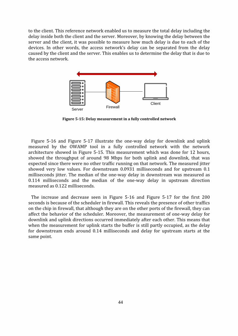
44

to the client. This reference network enabled us to measure the total delay including the delay inside both the client and the server. Moreover, by knowing the delay between the server and the client, it was possible to measure how much delay is due to each of the devices. In other words, the access network’s delay can be separated from the delay caused by the client and the server. This enables us to determine the delay that is due to the access network.

Figure 5-16 and Figure 5-17 illustrate the one-way delay for downlink and uplink measured by the OWAMP tool in a fully controlled network with the network architecture showed in Figure 5-15. This measurement which was done for 12 hours, showed the throughput of around 98 Mbps for both uplink and downlink, that was expected since there were no other traffic running on that network. The measured jitter showed very low values. For downstream 0.0931 milliseconds and for upstream 0.1 milliseconds jitter. The median of the one-way delay in downstream was measured as 0.114 milliseconds and the median of the one-way delay in upstream direction measured as 0.122 milliseconds.

The increase and decrease seen in Figure 5-16 and Figure 5-17 for the first 200 seconds is because of the scheduler in firewall. This reveals the presence of other traffics on the chip in firewall, that although they are on the other ports of the firewall, they can affect the behavior of the scheduler. Moreover, the measurement of one-way delay for downlink and uplink directions occurred immediately after each other. This means that when the measurement for uplink starts the buffer is still partly occupied, as the delay for downstream ends around 0.14 milliseconds and delay for upstream starts at the same point.

Client

ServerFirewall

Figure 5-15: Delay measurement in a fully controlled network

45

Figure 5-16: One-way Delay DL in a controlled network

Figure 5-17: One-way Delay UL in a controlled network

47

Chapter 6

Analyzing the Collected Data

The first question, which comes to mind when you want to select an Internet access subscription from different available ISPs, is whether you will experience good throughput as a function of the price that you are willing to pay. This question usually cannot be answered easily, since it depends on many different factors, although there are some websites, which a subscriber can use to measure the throughput of their existing Internet access network subscription. These websites are used by many users to learn the actual throughput of their Internet access network subscription. Unfortunately, this information is only available to you after you have made your selection and paid for your subscription. However, you can often look at the measurements made by others who are in “substantially the same situation”. Based on their measurements you may be able to infer what experience you will have if you subscribe to the same ISP as they have.

One of the obvious conclusions based upon the analysis of the measurements collected during this project, was that the available bandwidth and throughput that can be achieved by subscribers is usually less than what the providers advertise in their offer to their prospective customers. According to research done by S. Bauer et al. [70], one of the reasons for this is that the broadband access network infrastructure is frequently shared between several users, hence the capacity of the network will be shared by these users. The more users who share the network’s capacity, the less bandwidth is available for each user. However, it is worthy to mentioning that in some cases, our measurement results indicated that ISPs provided more bandwidth (i.e., higher peak data rates) than what they promised for the uplink direction, but almost never provide more bandwidth on the downlink.

More details will be discussed in the different case studies describe in the following sections.

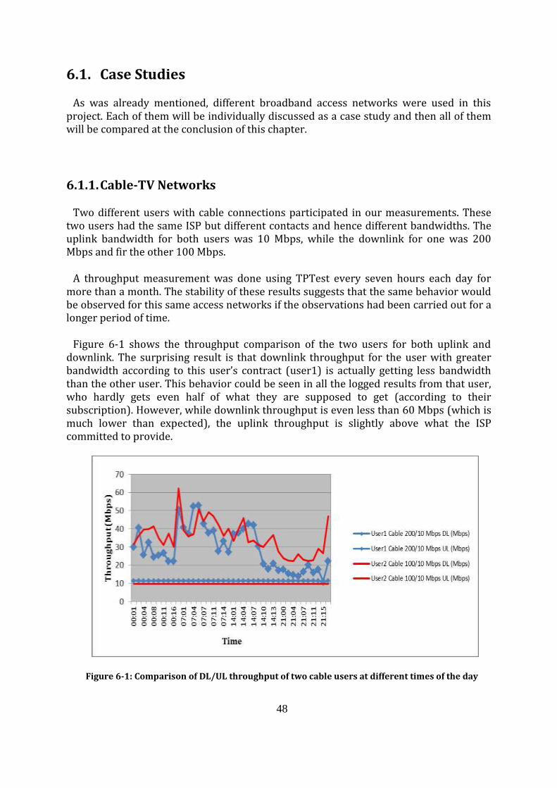
48

6.1. Case Studies

As was already mentioned, different broadband access networks were used in this project. Each of them will be individually discussed as a case study and then all of them will be compared at the conclusion of this chapter.

6.1.1. Cable-TV Networks

Two different users with cable connections participated in our measurements. These two users had the same ISP but different contacts and hence different bandwidths. The uplink bandwidth for both users was 10 Mbps, while the downlink for one was 200 Mbps and fir the other 100 Mbps.

A throughput measurement was done using TPTest every seven hours each day for more than a month. The stability of these results suggests that the same behavior would be observed for this same access networks if the observations had been carried out for a longer period of time.

Figure 6-1 shows the throughput comparison of the two users for both uplink and downlink. The surprising result is that downlink throughput for the user with greater bandwidth according to this user’s contract (user1) is actually getting less bandwidth than the other user. This behavior could be seen in all the logged results from that user, who hardly gets even half of what they are supposed to get (according to their subscription). However, while downlink throughput is even less than 60 Mbps (which is much lower than expected), the uplink throughput is slightly above what the ISP committed to provide.

Figure 6-1: Comparison of DL/UL throughput of two cable users at different times of the day

49

The time stamps shown in Figure 6-1 are for different times of the day (i.e., every 7 hours) and the measurements utilized TPTest. Each measurement made 5 sequential samples of throughput. This pattern of sampling is part of TPTest’s behavior.

Figure 6-2 shows a test1 by user1 of their uplink and downlink using one of the available websites that measures a user’s Internet connection’s characteristics. This user has a cable subscription to a Swedish ISP, for 200 Mbps for downlink and 10 Mbps for their uplink. According to the website, user1 gets roughly 162 / 11 Mbps for downlink/uplink respectively. However, the measurements collected over a longer time by our test bed indicate this user’s downlink results are consistently much lower, hence this subscriber should complain to their ISP that they are not getting the service that they have paid for.

As was shown in Figure 6-1, user 1 with a contract for 200/10 Mbps actually had a lower downlink throughput than user2 who has a contract for a 100/10 Mbps cable connection. Figure 6-2 illustrates the performance of this user’s connection throughput as measured by the Bredbandskollen web tool. This difference between actual throughput and the throughput which these network test tools provide, is due to the way these two ISP prioritize their packets to and from their own IP addresses, and as a result, packets which are coming from their own IP address domain are given higher priority, and hence achieve much better throughput. However, these values are not representative of the experience that the user will get when communicating with a node in another ISP’s network.

1 The test is done on http://www.bredbandskollen.se/ website.

Figure 6-2: Measurement of DL/UL throughput via a measuring website, for a cable user with 200/10 Mbps contract.

http://www.bredbandskollen.se/

50

Further analysis revealed that the problem with this user’s network throughput is the peering capacity between their ISP and the peering point through which traffic from the user must pass to reach our server. Peering traffic characteristics depend on the agreements between the providers. Peering enables providers to use each other’s networks and infrastructures to carry traffic to and from their own customers to and from other ISPs customers.

Evaluating the one-way delay of cable-users showed vastly different behaviors for downstream and upstream. Comparing the results of our measurements with the requirements for small cell transport, due to the fact that the upstream direction one-way delay would be several hundred milliseconds, such an access network does not fulfill the maximum 100 milliseconds delay of our requirements. This behavior was even more obvious for users with a very asymmetric bandwidth contract, such as user1 (shown in Figure 6-3), who had a contract for 200 Mbps downstream and 10 Mbps for upstream. Figure 6-3 and Figure 6-4 show the one-way delay for downstream and upstream directions (respectively) for the cable user with 200/10 Mbps bandwidth. As shown in these graphs, in the downstream direction a reasonable delay is achieved; however, in upstream direction high delays are observed.

There are several reasons for having low throughput and high upstream delay in cable networks. First of all, the bandwidth of this kind of network is shared between all the users who are connected to a given cable modem termination system [71]. This means adding one extra device by one of the subscribers in the shared network, will degrade the throughput for all other users. Additionally, as cable networks are radio-frequency (RF) networks [72], and use the same frequency spectrum as broadcast TV a jack for this network is vulnerable to letting in broadcast TV signals which can lead to transient impairments. Moreover, the upstream bandwidth is usually assigned very limited capacity by the service providers; hence, the competition with all of the other user’s traffic in the limited bandwidth of uplink direction results in low throughput, and hence high delays.

Figure 6-3 illustrates the one-way delay for downlink for a cable user with a contract of 200/10 Mbps. This measurement was performed at midnight, and shows a median 5.2 milliseconds as the downstream one-way delay. Figure 6-4 shows the one-way delay of the same user for uplink. The upstream measurement shows a median of 7.8 milliseconds one-way delay.

The point, which should be noted in regard to these two figures, is the range of the one-way delay on the vertical axis. The huge difference stems from the variation of one-way delay (i.e., jitter) in uplink and downlink separately. In other words, the downlink one-way jitter of 2.8 milliseconds and the uplink one-way jitter of 146 milliseconds with the difference of 143.2 milliseconds causing a big difference in range of the one-way delay between upstream and downstream. The reason for this huge difference is that a very limited bandwidth of the media is shared between all users for upstream link. As a result of the process of accessing the uplink channel leads to users waiting for a long time to get access to this uplink channel. This means that in order to send an uplink packet when competing with other users the process takes longer, hence making the one-way uplink delay longer.

51

Another point about Figure 6-3 and Figure 6-4 is the periodic spikes on both uplink and downlink directions. The reason for those spikes is discussed in section 6.2.5. Moreover, cable-TV access technology is a grant-based system, and that means the cable modem needs to send a request for the bandwidth to the Cable Modem Terminating System (CMTS), and then wait until it granted the bandwidth to use [73]. And in case of more active users, the waiting time will become longer, and that justifies the reason we have more one-way delay in cable-TV compare to fiber access technology.

Figure 6-3: One-way Delay DL for a Cable User with 200/10 Mbps DL/UL

52

6.1.2. ADSL/ADSL2+

ADSL technology uses the existing twisted pairs of copper telephone lines for transferring data traffic. Because more traffic flows in the downstream direction to users as compare to the upstream direction, ADSL allocates an asymmetric bandwidth for the signaling in these two different directions. According to ANSI T1.413-1998 Issue2 standard, the maximum bandwidth which can be offered by ADSL, is 8 Mbps for the downlink and 1 Mbps for uplink. In the best case ADSL2+ Annex M, offers up-to 24 Mbps for the downstream and 3.3 Mbps for upstream traffic (ITU G.992.5 Annex M). This means that ADSL technology does not support sufficient capacity in terms of link throughput (in comparison with the requirements stated in Table 1-1).

Figure 6-4: One-way Delay UL for a Cable User with 200/10 Mbps DL/UL

53

Figure 6-5 presents a comparison of throughput for two ADSL users with different subscriptions, who have different specified maximum upload and download data rates. (Both users have a maximum 1Mbps upload data rate, while one user has 7Mbps and the other 13Mbps download data rate.)

Assessing the one-way delay of ADSL(2+) users, we found acceptable delay for both upstream and downstream (with regard to our requirements in Table 1-1). Figure 6-6 and Figure 6-7 illustrate the one-way delay for downlink and uplink respectively, from the measurement performed at midnight (00:00). The median one-way delay of the downlink is 12.3 milliseconds and in uplink direction, the median one-way delay is 10.4 milliseconds.

Figure 6-5: Throughput of two ADSL Users at different times of the day

54

Figure 6-6: One-way Delay DL for an ADSL User

Figure 6-7: One-way Delay UL for an ADSL User

55

The periodic spikes shown in Figure 6-6 and Figure 6-7 have the same reason as described before for the other figures. However, the spikes are more visible for uplink direction in this case, and that is because we have very limited bandwidth for upstream in ADSL networks.

All the results from throughput and one-way delay measurements imply that the very asymmetric bandwidth provided by the ISPs can cause difficulties in synchronization and upstream capacity for ADSL access networks. This problem stems from the nature of ADSL networks as they can only provide low throughput in both uplink and downlink directions. Moreover, the difference in throughput between the downstream and upstream is too high which can cause high delays in the upstream direction. For example, on the days when important sport teams in a country have a match, the fans are most likely interested in uploading photos of the match and exchanging other kinds of news regarding the match via their social network sites. This means that a huge load of traffic will be flowing in upstream direction, thus having too much asymmetry can lead to a big delay from the users’ terminals to the server.

Apart from the above mentioned problem, the capacity which ADSL networks are able to provide is not sufficient to match the requirements of small cell deployments as stated in Table 1-1.

6.1.3. VDSL2

Three VDSL2 users participated in our measurement. These three users had three different bandwidths in their subscriptions with two ISPs in Sweden. Figure 6-8 shows the graph of their throughput, which was measured every 7 hours over the course of one day. As shown in the graph, user3 has a quite stable throughput for both downstream and upstream, while user1 and user2 have a lot of fluctuation in the downstream throughputs. This can be due to the continuous usage of Internet and extensive download requests for these two users.

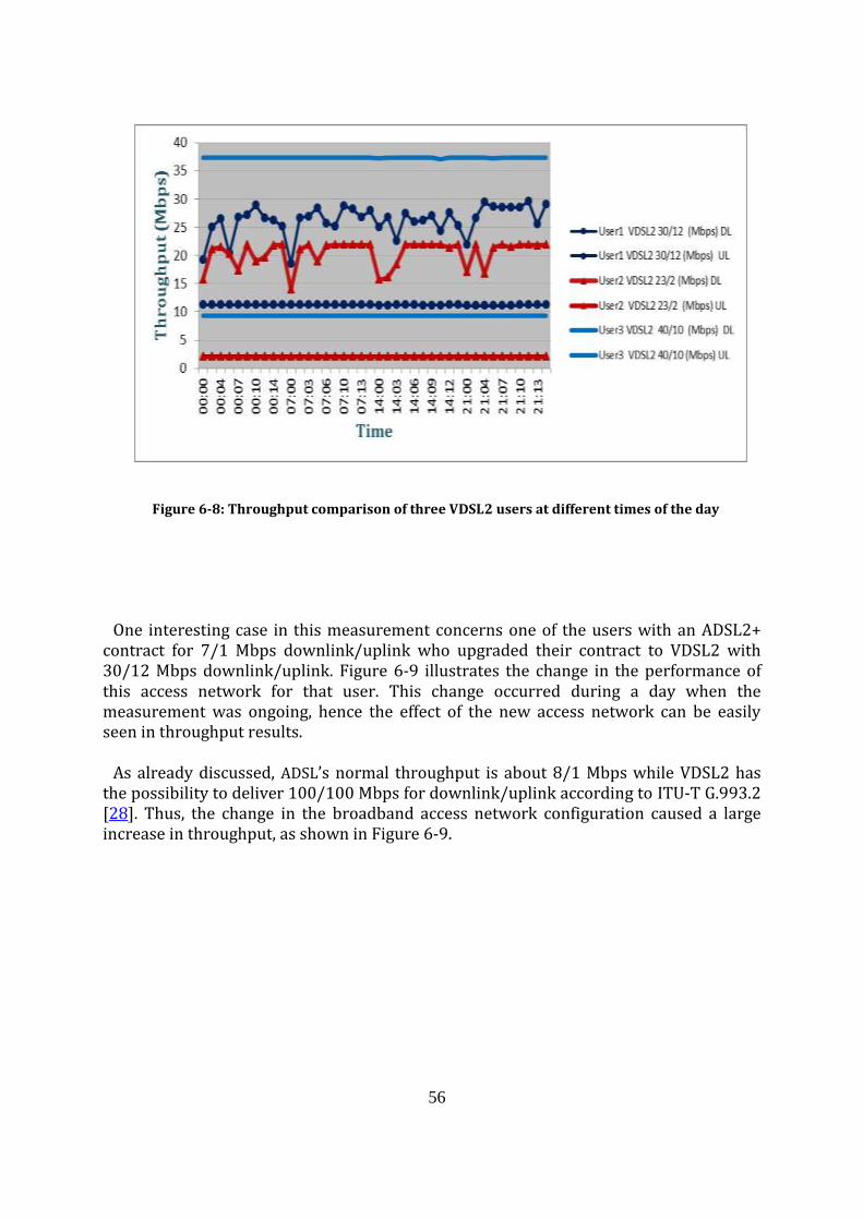
56

One interesting case in this measurement concerns one of the users with an ADSL2+ contract for 7/1 Mbps downlink/uplink who upgraded their contract to VDSL2 with 30/12 Mbps downlink/uplink. Figure 6-9 illustrates the change in the performance of this access network for that user. This change occurred during a day when the measurement was ongoing, hence the effect of the new access network can be easily seen in throughput results.

As already discussed, ADSL’s normal throughput is about 8/1 Mbps while VDSL2 has the possibility to deliver 100/100 Mbps for downlink/uplink according to ITU-T G.993.2 [28]. Thus, the change in the broadband access network configuration caused a large increase in throughput, as shown in Figure 6-9.

Figure 6-8: Throughput comparison of three VDSL2 users at different times of the day

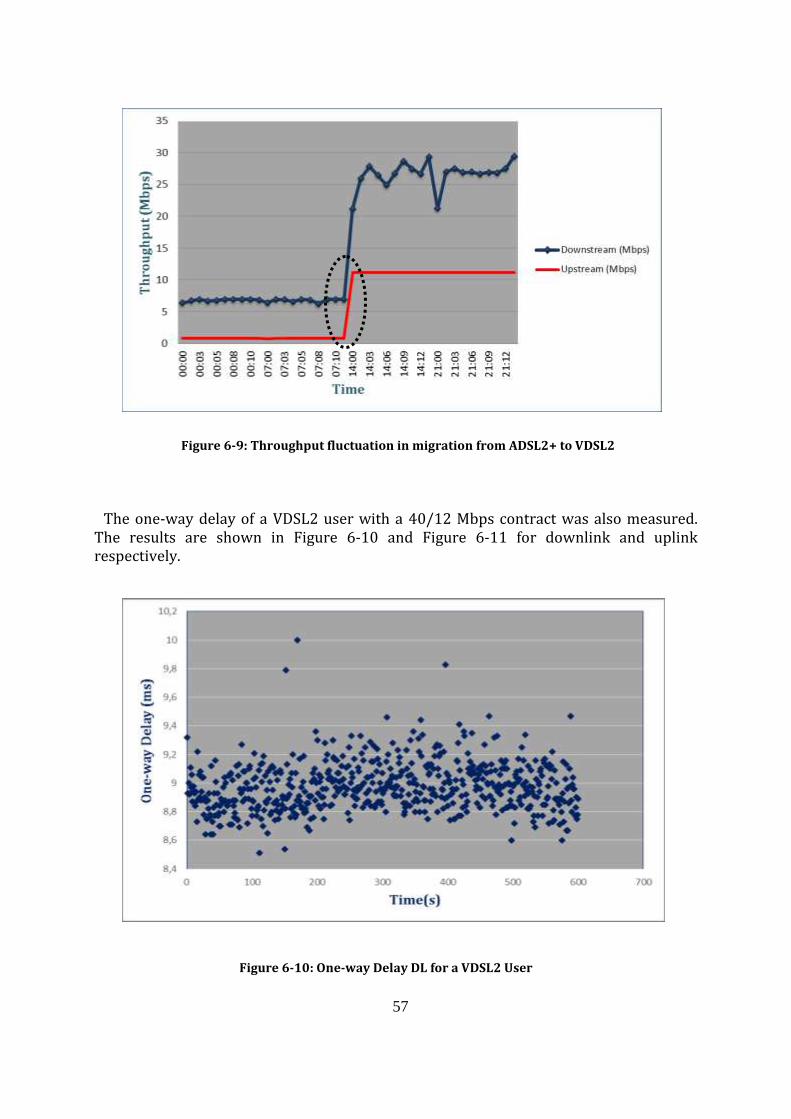
57

The one-way delay of a VDSL2 user with a 40/12 Mbps contract was also measured. The results are shown in Figure 6-10 and Figure 6-11 for downlink and uplink respectively.

Figure 6-9: Throughput fluctuation in migration from ADSL2+ to VDSL2

Figure 6-10: One-way Delay DL for a VDSL2 User

58

The median one-way delay for both downlink and uplink of VDSL2 users was measured and showed quite similar results. The median for downstream one-way delay was measured to be 9.105 milliseconds and the median for upstream one-way delay was measured as 9.175 milliseconds. In order to explain this similarity of one-way delay for both uplink and downlink, it should be noted that most of the delay in VDSL2 networks is because of the line coding itself, therefore, the serialization delay has less impact. For this reason, upstream and downstream delays are almost symmetric.

Figure 6-11: One-way Delay UL for a VDSL2 User

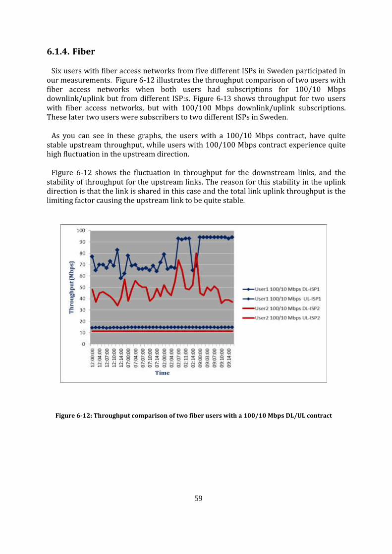
59

6.1.4. Fiber

Six users with fiber access networks from five different ISPs in Sweden participated in our measurements. Figure 6-12 illustrates the throughput comparison of two users with fiber access networks when both users had subscriptions for 100/10 Mbps downlink/uplink but from different ISP:s. Figure 6-13 shows throughput for two users with fiber access networks, but with 100/100 Mbps downlink/uplink subscriptions. These later two users were subscribers to two different ISPs in Sweden.

As you can see in these graphs, the users with a 100/10 Mbps contract, have quite stable upstream throughput, while users with 100/100 Mbps contract experience quite high fluctuation in the upstream direction.

Figure 6-12 shows the fluctuation in throughput for the downstream links, and the stability of throughput for the upstream links. The reason for this stability in the uplink direction is that the link is shared in this case and the total link uplink throughput is the limiting factor causing the upstream link to be quite stable.

Figure 6-12: Throughput comparison of two fiber users with a 100/10 Mbps DL/UL contract

60

Figure 6-13 shows fluctuation in throughput for two other users with symmetric bandwidth (100/100 Mbps)and from two different ISP:s. Despite the Figure 6-12, this figure shows a fluctuation of both downlink and uplink due to the other competing traffics in the network. In other words, the aggregation network bandwidth is shared between different users, hence the upstream link fluctuates quite a bit.

One-way delay has been also measured for both groups of users, i.e., users with 100/10 Mbps DL/UL and users with 100/100 Mbps DL/UL contracts. Figure 6-14 and Figure 6-15 show the one-way delay for users with asymmetric networks, and Figure 6-16 and Figure 6-17 present the one-way delay for symmetric networks with 100/100 Mbps DL/UL. These figures illustrate the correlation of throughput and one-way delay.

Table 6-1 shows a comparison of the median one-way delay for 100/10 and 100/100 Mbps fiber access networks. This table shows that for different connections on network, different delays might achieve. This means that we cannot make any conclusions of the correlation of delay and throughput here, since each connection depending on many factors on the network can get different amount of delay.

Figure 6-13: Throughput comparison of two Fiber users with 100/100 Mbps DL/UL contract

61

Table 6-1: One-way delay and throughput for fiber users

Figure 6-14 and Figure 6-15 show graphs of one-way delay for downlink and uplink of users with asymmetric bandwidths (100/10 Mbps).

In the downstream direction, the majority of the measured delay is less than five milliseconds of one-way delay over a period of 10 minutes.

The reason(s) for the spikes shown in Figure 6-14, Figure 6-15, Figure 6-16, and Figure 6-17 are not known. Determining the reason(s) for these spikes is left as future work.

One-way Delay Median for

DL (ms) One-way Delay Median for

UL (ms)

Fiber User with 100/10 Mbps DL/UL

2.13 0.73

Fiber User with 100/100 Mbps DL/UL

5.47 1.22

62

Figure 6-14: One-way Delay DL for a Fiber User with 100/10 Mbps DL/UL

Figure 6-15: One-way Delay UL for a Fiber User with 100/10 Mbps DL/UL

63

Figure 6-17: One-way Delay UL for a Fiber User with 100/100 Mbps DL/UL

Figure 6-16: One-way Delay DL for a Fiber User with 100/100 Mbps DL/UL

64

6.2. Discussion

After discussing all the individual case studies in our measurements, the overall findings and some comparisons of results regarding the different access networks will now be presented.

6.2.1. Avoiding congestion in backhaul networks

As mentioned earlier in some of the measurements, we found that there is congestion in the backhaul networks. In order to avoid that congestion, we came up with an idea, which led to a patent filing (Methods and Nodes for handling congestion in Backhaul Networks). This is viewed by the company as a valuable result of this thesis project. The detailed description of the patent will be publicly available 18 months after the registration date. The abstract of this patent application is:

“The present invention relates to nodes and method in such nodes of a Radio Access Network or a Backhaul Network connected to the Radio Access Network comprising a number of Radio Base Station nodes being connected to the Backhaul Network comprising communication paths for transferring data packets. There are nodes configured to support the performing of a method involving receiving a notification indicating congestion in one or more data paths of the Backhaul Network and deciding based on current radio information and data path information to initiate handover of data packet traffic from one Radio Base Station to another Radio Base Station for solving the congestion problem in the indicated one or more data communication paths.”

6.2.2. Correlation of Bandwidth and One-way Delay

Table 6-2 shows a comparison between the different broadband access networks in terms of one-way delay. In this comparison, “fiber” has the lowest median one-way delay for both uplink and downlink, while “ADSL” has the highest one-way delay in both directions. However, an important point, which should be noted here, is that the type of broadband access network selected depends on the needs of the user and their purpose for their usage. Hence, depending on the user’s needs, a “cable” access network might be the best option in one location while “fiber” is the best option for another purpose or in another location.

65

Table 6-2: Comparison of one-way delay between different broadband access networks

Cable ADSL2+ VDSL2 Fiber

Median one-way delay DL

(ms) 6.90 12.15 9.10 2.13

Median one-way delay UL

(ms) 6.84 11.65 9.17 0.73

According to the above results, the alternative broadband access networks can be categorized in the following order (from lowest to highest) from a one-way delay perspective: Fiber<Cable<VDSL2<ADSL2+.

6.2.3. Correlation between the Number of Hops and One-way Delay

The number of hops (i.e., the number of routers through which packets must pass through) between the server and each of the clients in our measurement have been measured using the OWAMP tool, as part of the report for our one-way delay measurement, and via “traceroute” which provides the exact IP address of all the routers on the way from the server to the clients. It worth mentioning that some ISPs do not allow traceroute packets to propagate the whole way along. This means that in this case only a certain number of routers will be presented in traceroute report. However, since OWAMP was used in this measurement, the exact number of hops could be determined for each of the clients.

Table 6-3: One-way delay with number of hops for different broadband access networks

Cable ADSL VDSL Fiber

Number of Routers (Hops)

10 12 11 11

Median one-way delay DL

(ms) 6.90 12.15 9.10 2.13

66

Table 6-3 shows the correlation of the number of hops (i.e., the number of routers between client and server), and the one-way downlink delay for different broadband access networks. As it can be deduced from these figures, since the number of hops are nearly equal, we can make conclusion that access media has a great impact on delay, and number of hops has a limited impact on delay.

6.2.4. Investigation of One-way Delay behavior for a random user

As mentioned before the measurements in this thesis project were done every seven hours, to make sure we cover different times of the day. Below the one-way delay for a random day are shown for a random user having a “fiber” connection (specifically 100/100 Mbps) is illustrated.

Figure 6-18: One-way Delay for UL and DL- Fiber Network- Time of day 00:00

67



68

As it is shown in the above graphs, the uplink one-way delay is consistently greater than the downlink one-way delay for all four times of the day. This means that in the downstream direction the aggregation network has more capacity allocated than is in use (hence there is no congestion in this part of the network). As noted earlier, the reason(s) for these delay spikes are not known.

Figure 6-22 shows all four time-slots measurements in a single graph. The comparison of the one-way delays in this figure, indicates the frequent spikes in high uplink one-way delay at 14:00.


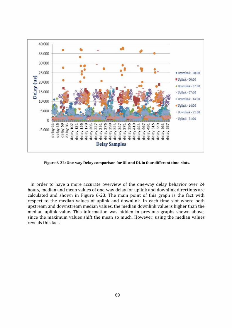
69

In order to have a more accurate overview of the one-way delay behavior over 24 hours, median and mean values of one-way delay for uplink and downlink directions are calculated and shown in Figure 6-23. The main point of this graph is the fact with respect to the median values of uplink and downlink. In each time slot where both upstream and downstream median values, the median downlink value is higher than the median uplink value. This information was hidden in previous graphs shown above, since the maximum values shift the mean so much. However, using the median values reveals this fact.

Figure 6-22: One-way Delay comparison for UL and DL in four different time-slots.

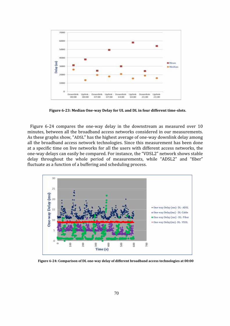
70

Figure 6-24 compares the one-way delay in the downstream as measured over 10 minutes, between all the broadband access networks considered in our measurements. As these graphs show, “ADSL” has the highest average of one-way downlink delay among all the broadband access network technologies. Since this measurement has been done at a specific time on live networks for all the users with different access networks, the one-way delays can easily be compared. For instance, the “VDSL2” network shows stable delay throughout the whole period of measurements, while “ADSL2” and “fiber” fluctuate as a function of a buffering and scheduling process.

Figure 6-23: Median One-way Delay for UL and DL in four different time-slots.

Figure 6-24: Comparison of DL one-way delay of different broadband access technologies at 00:00

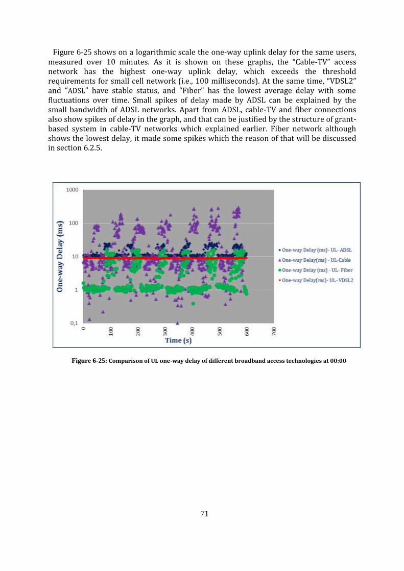
71

Figure 6-25 shows on a logarithmic scale the one-way uplink delay for the same users, measured over 10 minutes. As it is shown on these graphs, the “Cable-TV” access network has the highest one-way uplink delay, which exceeds the threshold requirements for small cell network (i.e., 100 milliseconds). At the same time, “VDSL2” and “ADSL” have stable status, and “Fiber” has the lowest average delay with some fluctuations over time. Small spikes of delay made by ADSL can be explained by the small bandwidth of ADSL networks. Apart from ADSL, cable-TV and fiber connections also show spikes of delay in the graph, and that can be justified by the structure of grant-based system in cable-TV networks which explained earlier. Fiber network although shows the lowest delay, it made some spikes which the reason of that will be discussed in section 6.2.5.

Figure 6-25: Comparison of UL one-way delay of different broadband access technologies at 00:00

72

6.2.5. Spikes in one-way delay

As you might have noticed in the graphs presented in previous sections, we got some

periodic spikes on one-way delay graphs for ADSL, cable-TV, and fiber broadband access

technologies. In order to find out the reasons of having such behavior in one-way delay we

did some investigations by considering various factors which might have affected our results.

Our first thought was the NTP-daemon (NTPD) and GPS-daemon (GPSD) synchronization

time could be the cause of the spikes.. However, GPSD is updated every second and NTPD in

both server and clients is updated every 16 seconds, hence if this time synchronization was

the reason of periodic spikes, we would have much shorter periods of spikes while the spikes

in our results are occurring around every 100 seconds. As a result, this source was ruled out as

the reason for these periodic spikes in one-way delay.

Our next thought was that the spikes might be the effect of dynamic host configuration

protocol (DHCP) address renewal. However, the DHCP time for clients is usually much

longer than the 100 seconds periods that the spikes occurred in our case. Moreover, depending

on the ISP, they utilize lease time in range of one to several hours, and since the renewal time

is half of the lease time, so the spikes would have had periods of at least 30 minutes. Hence,

this source was also ruled out.

The third assumption was address resolution protocol (ARP) cache flush, which might have

caused the periodic spikes. According to RFC1122 [74], there are four different techniques

which are used to flush the ARP cache. In one of these methods, the cache data times out

periodically, even if the cache entries are in use and some traffic is outgoing. This behavior is

exactly what we see in our measurement results for fiber, cable-TV, and ADSL(2+)

broadband access technologies, and in our case around every 100 seconds such an update

occurs. Now the question is that why the same kind of spikes are not seen in VDSL2 test

results. The answer to this question is that the cache flushes still occur in VDSL2, but if the

VDSL2 modem is sending a gratuitous ARP for itself, then the cache will be refreshed much

quicker. In our VDSL2 measurement, the spikes occur in microseconds range.

73

Chapter 7

Conclusions

This chapter will discuss the conclusions resulting from this thesis, and will give some suggestions for possible future work, which could be conducted by people interested in this area of research.

7.1. Conclusions

Results of the measurements done in this thesis project first revealed an obvious fact that users never get the promised bandwidth promised by their ISPs. This fact was most visible for the downlink bandwidth rather than the uplink bandwidth. Some ISPs do not promise a specific bandwidth to users and instead specify data rates for “up to” a specific peak data rates. This way they do not give their customers grounds to complain about the throughput they actually experience. One of the other conclusions we make after doing a wide range of measurements is that although we expected to see a bottleneck in the “last mile”, we noticed that in some networks this is not where the bottleneck actually is. For instance, in one of the ISP’s network, the bottleneck was the peering interconnection, and in some other cases with 100 Mbps service, the bottleneck appeared to be in somewhere in the operator’s aggregation or core network.

An interesting result of this thesis project, which was the main goal of doing all of these measurements, is the conclusion concerning different broadband access technologies that could be used as backhaul transport for small cell deployment. As mentioned earlier, four different broadband access networks were tested in the measurements reported in this thesis. By comparing these results we could compare their performance with the backhaul requirements of small cell networks as given by Ericsson, the possibility of accepting or rejecting each of these alternative networks will be discussed in detail in a subsequent subsection.

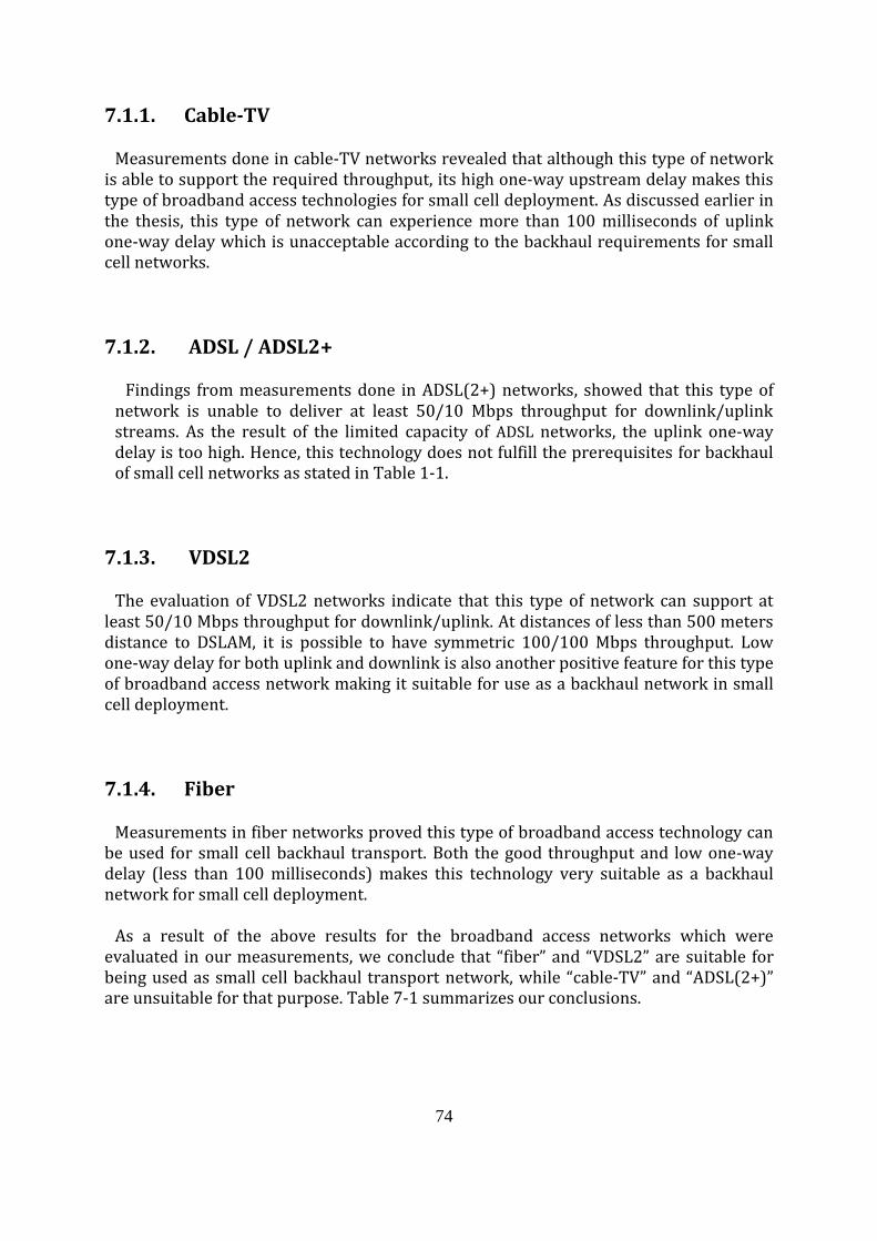
74

7.1.1. Cable-TV

Measurements done in cable-TV networks revealed that although this type of network is able to support the required throughput, its high one-way upstream delay makes this type of broadband access technologies for small cell deployment. As discussed earlier in the thesis, this type of network can experience more than 100 milliseconds of uplink one-way delay which is unacceptable according to the backhaul requirements for small cell networks.

7.1.2. ADSL / ADSL2+

Findings from measurements done in ADSL(2+) networks, showed that this type of network is unable to deliver at least 50/10 Mbps throughput for downlink/uplink streams. As the result of the limited capacity of ADSL networks, the uplink one-way delay is too high. Hence, this technology does not fulfill the prerequisites for backhaul of small cell networks as stated in Table 1-1.

7.1.3. VDSL2

The evaluation of VDSL2 networks indicate that this type of network can support at least 50/10 Mbps throughput for downlink/uplink. At distances of less than 500 meters distance to DSLAM, it is possible to have symmetric 100/100 Mbps throughput. Low one-way delay for both uplink and downlink is also another positive feature for this type of broadband access network making it suitable for use as a backhaul network in small cell deployment.

7.1.4. Fiber

Measurements in fiber networks proved this type of broadband access technology can be used for small cell backhaul transport. Both the good throughput and low one-way delay (less than 100 milliseconds) makes this technology very suitable as a backhaul network for small cell deployment.

As a result of the above results for the broadband access networks which were evaluated in our measurements, we conclude that “fiber” and “VDSL2” are suitable for being used as small cell backhaul transport network, while “cable-TV” and “ADSL(2+)” are unsuitable for that purpose. Table 7-1 summarizes our conclusions.

75

Table 7-1: Suitability of different broadband access networks to be used for small cell transport

Broadband Access Networks Suitable for small cell backhaul transport

Cable-TV No

ADSL(2+) No

VDSL2 Yes

Fiber Yes

7.2. Future Work

The following recommendations are given for future work:

- Trial and verifying of the requirements with real small cell base stations. - Continue improvements to one of the measurement tools “BART”. Although some

improvements were initiated due to results of the measurements performed in this thesis project because we found that this tool produced results were not trustworthy. As a result, we had to use alternative tools for our measurements.

- Investigation of other possible criteria which might affect the network delay, which made spikes on our measurement results.

- There needs to be realistic implementation of the patented idea to avoid the congestion in backhaul networks.

- Finally, investigation and implementation of handovers between small cell base stations needs to be done to and from Wi-Fi and 3G and LTE technologies.

76

7.3. Required Reflections

The results of the measurements done in this thesis had an economic contribution in sense of helping telecommunication companies to invest in their current transport network systems, which have the potential to be used as small cell backhaul, rather than requiring the introduction of new transport solutions which would be costly. Considering the ethical aspects, the identities of the ISPs involved in measurements of this thesis were not disclosed, since the purpose of this thesis project was to investigate the behavior of different access technologies, and identifying the best or the worst ISP was not the goal of this thesis.

Enhancing the quality of transport in small cell networks based the research and

measurements done in this thesis project should help improve the end-user’s experience,

which is a social contribution of this thesis. Furthermore, investigation and analysis of the

different types of broadband access networks gives end-users better understanding of the

actual performance provided by their Internet network access subscriptions.

Having a good picture of each of the broadband access technologies can offer more options to choose between in different situations. As an example upgrading to VDSL2 from ADSL2+ network could eliminate the need of many business trips to meetings as very good video conference services can be offered. Also upgrading to a fiber connection with 1 Gbps in future may provide an environmental contribution as such an access network can reduce the impact on the environment by reducing the usage of resources such as fuel and carbon oxide, and preventing air pollution.

77

References

[1] "3GPP specification: 21.905.", [Online],Available:http://www.3gpp.org/ftp/Spec s/html-info/21905.htm, 2013-08-06,13:56:33. [Accessed: 07-Aug-2013].

[2] “Ericsson, Internal document.”

[3] J. P. Pereira and J. A. Pires, “Broadband access technologies evaluation tool (BATET),” Technological and Economic Development. 13(4):288-294, January 2007. DOI:10.1080/13928619.2007.9637814 .

[4] S. Machiraju, D. Veitch, F. Baccelli, and J. C. Bolot, “Adding definition to active probing,” SIGCOMM Comput. Commun. Rev., vol. 37, no. 2, pp. 17–28, Mar. 2007.

[5] P. Legonkov and V. Prokopov, “Small Cell Wireless Backhaul in Mobile Heterogeneous Networks,” Master's thesis, KTH, Royal Institute of Technology, School of Information and Communication Technology, TRITA-ICT-EX- 2012:129,July2012,Available:http://urn.kb.se/resolve?urn=urn:nbn:se:kth:diva-99010.

[6] K. Lee, J. Lee, Y. Yi, I. Rhee, and S. Chong, “Mobile data offloading: how much can WiFi deliver?,” in Proceedings of the 6th International Conference, New York, NY, USA, 2010, pp. 26:1–26:12.

[7] M. M. da Silva, Multimedia Communications and Networking. CRC Press, Taylor & Francis Group, ISBN 978-1-4665-5929-2, eBook, 2012.

[8] J. Korhonen, Introduction to 3G mobile communications. Artech House Mobile Communication Series, Second Edition, ISBN 1-58053-507-0, 2003.

[9] R. Prasad, C. Dovrolis, M. Murray, and K. Claffy, “Bandwidth estimation: metrics, measurement techniques, and tools,” Network, IEEE, vol. 17, no. 6, pp. 27 – 35, Dec. 2003.

[10] C. Le Thanh Man, G. Hasegawa, and M. Murata, “A Merged Inline Measurement Method for Capacity and Available Bandwidth,” in Passive and Active Network Measurement, vol. 3431, C. Dovrolis, Ed. Springer Berlin / Heidelberg, 2005, pp. 341–344.

[11] B. Melander, Probing-Based Approaches to Bandwidth Measurements and Network Path Emulation. Acta Universitatis Upsaliensis, 2002.

http://www.3gpp.org/ftp/Spec%20s/html-info/21905.htm

http://www.3gpp.org/ftp/Spec%20s/html-info/21905.htm

http://urn.kb.se/resolve?urn=urn:nbn:se:kth:diva-99010


78

[12] E. Bergfeldt, “Available-Bandwidth Estimation in Packet-Switched Communication Networks,”, Dissertation, Linköpings Universitet, Institutionen för teknik och naturvetenskap. ISBN 978-91-7393-292-9, 174 pages, Available: http://liu.diva-portal.org/smash/get/diva2:358574/FULLTEXT01, 2010.

[13] D. Mills, J. Martin, J. Burbank, and W. Kasch, “RFC 5905: Network Time Protocol version 4: Protocol and algorithms specification,” Internet Engineering Task Force, 2010.

[14] Symmetricom, IEEE 1588 Precise Time Protocol: The new standard in time synchronization, white paper, Symmetricom, WP/IEEE 1588/1005/PDF, 2005, Available:http://www.syncworks.com/pdf/symmetricom-timeprovider-5000/IEEE_1588_Precise_Time_Protocol.pdf .

[15] A. Hernandez and E. Magafia, “One-way Delay Measurement and Characterization,” in Third International Conference on Networking and Services, 2007. ICNS, 2007, p. 114.

[16] G. Almes, S. Kalidindi, and M. Zekauskas, “RFC 2679: A one-way delay metric for IPPM,” Internet Society (Sep. 1999), pp. 1–20, 1999.

[17] L. Martini, E. Rosen, N. El-Aawar, T. Smith, and G. Heron, ‘Pseudowire Setup and Maintenance Using the Label Distribution Protocol (LDP)’, Internet Request for Comments, vol. RFC 4447 (Proposed Standard), Apr. 2006 [Online]. Available: http://www.rfc-editor.org/rfc/rfc4447.txt.

[18] B. Singh, “Outage probability analysis in soft handover for 3G wireless networks,”, 6th IEE International Conference on 3G and Beyond, 2005, vol. 2005, p.1-5.

[19] G. Almes, S. Kalidindi, and M. Zekauskas, ‘A One-way Packet Loss Metric for IPPM’, Internet Request for Comments, vol. RFC 2680 (Proposed Standard), Sep. 1999 [Online]. Available: http://www.rfc-editor.org/rfc/rfc2680.txt.

[20] M. Dischinger, A. Haeberlen, K. P. Gummadi, and S. Saroiu, “Characterizing residential broadband networks,” in Internet Measurement Conference: Proceedings of the 7 th ACM SIGCOMM conference on Internet measurement, 2007, vol. 24, pp. 43–56.

[21] N. Hu and P. Steenkiste, “Evaluation and characterization of available bandwidth probing techniques,” IEEE Journal on Selected Areas in Communications, vol. 21, no. 6, pp. 879–894, 2003.

[22] “DOCSIS®.” [Online]. Available: http://www.cablelabs.com/cablemodem/. [Accessed: 07-Aug-2013].

http://liu.diva-portal.org/smash/get/diva2:358574/FULLTEXT01

http://www.syncworks.com/pdf/symmetricom-timeprovider-5000/IEEE_1588_Precise_Time_Protocol.pdf

http://www.syncworks.com/pdf/symmetricom-timeprovider-5000/IEEE_1588_Precise_Time_Protocol.pdf

http://www.rfc-editor.org/rfc/rfc4447.txt


http://www.cablelabs.com/cablemodem/

79

[23] D. C. Yen, D. C. Chou, and J.-C. Wang, “DSL: the promising standard for new Internet era,” Computer Standards & Interfaces, vol. 23, no. 1, pp. 29–37, Mar. 2001.

[24] M. Dischinger, “Making broadband access networks transparent to researchers, developers, and users,”, Max Planck Institute for Software Systems, Dissertation, October 2010, Available: http://www.mpi-sws.org/~mdischin/papers/10_thesis.pdf

[25] A. Azzam and N. Ransom, Broadband access technologies. McGraw-Hill, 1999.

[26] D. Kagklis, S. Androulidakis, G. Patikis, and T. Doukoglou, “A comparative Performance Evaluation of the ADSL2+ and ADSL Technologies,” National Technical University of Athens (NTUA), Department of Electrical & Computer Engineering, 2005.

[27] M. Freire, M. M. Freire, and M. Periera, Encyclopedia of Internet Technologies and Applications. Idea Group Inc (IGI), 2008.

[28] “Press Release on New ITU Standard Delivers 10x ADSL Speeds.” [Online]. Available: http://www.itu.int/newsroom/press_releases/2005/06.html. [Accessed: 09-Jun-2013].

[29] Telia, “Abonnemang via fiber eller telejacket - Bredband - Privat - Telia.se.” [Online]. Available: http://www.telia.se/privat/bredband/abonnemang/. [Accessed: 09-Jun-2013].

[30] Z. Xiong, Socio-economic Impact of Fiber to the Home in Sweden. , Master's thesis, KTH Royal Institute of Technology, School of Information and Communication Technology, TRITA-ICT-EX-2013:35, February 2013, Available: http://urn.kb.se/resolve?urn=urn:nbn:se:kth:diva-118777.

[31] R. E. Wagner, J. R. Igel, R. Whitman, M. D. Vaughn, A. B. Ruffin, and S. Bickham, “Fiber-Based Broadband-Access Deployment in the United States,” Lightwave Technology, Journal of, vol. 24, no. 12, pp. 4526 –4540, Dec. 2006.

[32] J. S. Shaik and N. R. Patil, “FTTH deployment options for telecom operators,” Sterlite Optical Technologies Ltd., White Paper, pp. 1–9, 2005.

[33] J. Baker, T. Cagenius, C. Goodwin, M. Hansson, and M. Hatas, “Deep-fiber broadband access networks,” Ericsson Review, vol. 84, p. 1, 2007.

[34] J. Jing and Z. Xuesong, “Research on EPON of broadband access technology and broadband network deployment,” in Advanced Computer Theory and Engineering (ICACTE), 2010 3rd International Conference on, 2010, vol. 3, pp. V3–148 –V3–152.

http://www.mpi-sws.org/~mdischin/papers/10_thesis.pdf

http://www.mpi-sws.org/~mdischin/papers/10_thesis.pdf

http://www.itu.int/newsroom/press_releases/2005/06.html

http://www.telia.se/privat/bredband/abonnemang/


80

[35] L. Zhu, X. Fan, and Y. He, “New broadband access technology: Ethernet passive optical network (EPON),” Proceedings of SPIE, vol. 5282, no. 1, pp. 182–192, Apr. 2004.

[36] G. Kramer and G. Pesavento, “Ethernet passive optical network (EPON): building a next-generation optical access network,” Communications Magazine, IEEE, vol. 40, no. 2, pp. 66 –73, Feb. 2002.

[37] L. Khermosh, ‘Managed Objects of Ethernet Passive Optical Networks (EPON)’, Internet Request for Comments, vol. RFC 4837 (Proposed Standard), Jul. 2007 [Online]. Available: http://www.rfc-editor.org/rfc/rfc4837.txt.

[38] H. Li, R. Zheng, and A. Farrel, “Multi-Segment Pseudowires in Passive Optical Networks.” [Online]. Available: http://tools.ietf.org/search/draft-li-pwe3-ms-pw-pon-00#section-3. [Accessed: 28-Jun-2012].

[39] G. Santos-Boada and J. Domingo-Pascual, “Quality of Service in Multioperator GPON Access Networks with Triple-Play Services,” World Academy Of Science, Engineering And Technology, vol. 18, 2006.

[40] P. Jacquet, P. Mühlethaler, and P. Robert, “Framing protocols on upstream channel in CATV networks: asymptotic average delay analysis,”, INRIA Rocquencourt, RR-4114, inria-00072517, version 1, 2001, Available: http://hal.inria.fr/inria-00072517/PDF/RR-4114.pdf .

[41] M. S. Kuran and T. Tugcu, “A survey on emerging broadband wireless access technologies,” Computer Networks, vol. 51, no. 11, pp. 3013–3046, 2007.

[42] L. Nuaymi, WiMAX: Technology For Broadband Wireless Access. John Wiley and Sons, 2007.

[43] A. Ghosh, D. R. Wolter, J. G. Andrews, and R. Chen, “Broadband wireless access with WiMax/802.16: current performance benchmarks and future potential,” Communications Magazine, IEEE, vol. 43, no. 2, pp. 129 –136, Feb. 2005.

[44] V. Moeyaert and G. Maier, “Network technologies for broadband access,” in Transparent Optical Networks (ICTON), 2011 13th International Conference on, 2011, pp. 1 –5.

[45] W. Lehr and L. W. McKnight, “Wireless Internet access: 3G vs. WiFi?,” Telecommunications Policy, vol. 27, no. 5–6, pp. 351–370, Jun. 2003.

[46] A. Kumar, J. Sengupta, and Y. Liu, “3GPP LTE: The Future of Mobile Broadband,” Wireless Personal Communications, vol. 62, no. 3, pp. 671–686, 2012.

[47] N. L. Ewald, G. Fairhurst, N. Race, T. Baker, and P. Skoutaridis, “Next generation satellite broadband enablers,” in Telecom World (ITU WT), 2011 Technical Symposium at ITU, 2011, pp. 39 –44.


http://tools.ietf.org/search/draft-li-pwe3-ms-pw-pon-00%23section-3

http://tools.ietf.org/search/draft-li-pwe3-ms-pw-pon-00%23section-3

http://hal.inria.fr/inria-00072517/PDF/RR-4114.pdf

81

[48] J. P. Pereira and J. A. Pires, “Broadband access technologies,” 2007. [Online]. Available: http://bibliotecadigital.ipb.pt/handle/10198/1574. [Accessed: 18-Jun-2012].

[49] M. Hasib and J. A. Schormans, “Limitations of passive & active measurement methods in packet networks,” in Proceedings of LCS 2003 London Communications Symposium, London, 8th-9th September, 2003.

[50] L. Angrisani, S. D’Antonio, M. Vadursi, and G. Ventre, “Performance comparison of different techniques for available bandwidth measurement in packet switched network,” in 2003 IEEE International Symposium on Virtual Environments, Human-Computer Interfaces and Measurement Systems, 2003. VECIMS ’03, 2003, pp. 212 – 217.

[51] A. Tirumala, L. Cottrell, and T. Dunigan, “Measuring end-to-end bandwidth with Iperf using Web100,” in Web100”, Proc. of Passive and Active Measurement Workshop, 2003, p. 2003.

[52] D. Yin, E. Yildirim, and T. Kosar, “A data throughput prediction and optimization service for widely distributed many-task computing,” in Proceedings of the 2nd Workshop on Many-Task Computing on Grids and Supercomputers, New York, NY, USA, 2009, pp. 4:1–4:10.

[53] E. Yildirim, I. H. Suslu, and T. Kosar, “Which network measurement tool is right for you? a multidimensional comparison study,” in Proceedings of the 2008 9th IEEE/ACM International Conference on Grid Computing, Washington, DC, USA, 2008, pp. 266–275.

[54] S. Shalunov, B. Teitelbaum, A. Karp, J. Boote, and M. Zekauskas, “RFC 4656: A One-way Active Measurement Protocol (OWAMP),” Internet Engineering Task Force, 2006.

[55] K. Stangherlin, R. C. Filho, W. Lautenschlager, V. Guadagnin, L. Balbinot, R. Balbinot, and V. Roesler, “One-way delay measurement in wired and wireless mobile full-mesh networks,” in 2011 IEEE Wireless Communications and Networking Conference (WCNC), 2011, pp. 1044 –1049.

[56] Z. Shu and K. Kobayashi, “HOTS: An OWAMP-Compliant Hardware Packet Timestamper,” Passive and Active Network Measurement, pp. 358–361, 2005.

[57] K. Hedayat, R. Krzanowski, A. Morton, K. Yum, and J. Babiarz, ‘A Two-Way Active Measurement Protocol (TWAMP)’, Internet Request for Comments, RFC 5357 (Proposed Standard), Oct. 2008 [Online]. Available: http://www.rfc-editor.org/rfc/rfc5357.txt.

http://bibliotecadigital.ipb.pt/handle/10198/1574



82

[58] S. Ekelin, M. Nilsson, E. Hartikainen, A. Johnsson, J.-E. Mangs, B. Melander, and M. Bjorkman, “Real-Time Measurement of End-to-End Available Bandwidth using Kalman Filtering,” in Network Operations and Management Symposium, 2006. NOMS 2006. 10th IEEE/IFIP, 2006, pp. 73–84.

[59] “TPTEST.” [Online]. Available: http://tptest.sourceforge.net/about.php. [Accessed: 21-Feb-2013].

[60] L.-P. G. Hansen and I. C. Østhus, “NPT Online Broadband Test Tool,”, Master's thesis, NTNU, Norwegian University of Science and Technology, Department of Telematics,2009,Available:http://daim.idi.ntnu.no/masteroppgaver/004/4619/masteroppgave.pdf.

[61] T. Anjali, C. Scoglio, L. C. Chen, I. F. Akyildiz, and G. Uhl, “ABEst: an available bandwidth estimator within an autonomous system,” in IEEE Global Telecommunications Conference, 2002. GLOBECOM ’02, 2002, vol. 3, pp. 2360 – 2364 vol.3.

[62] “Performance Measurement Tools Taxonomy.”, CAIDA, The Cooperative Association for internet Data Analysis, [Online]. Available: http://www.caida.org/tools/taxonomy/performance.xml. [Accessed: 12-Mar-2013].

[63] J. Strauss, D. Katabi, and F. Kaashoek, “A Measurement Study of Available Bandwidth Estimation Tools,” in In IMC, 2003, pp. 39–44.

[64] M. Jain and C. Dovrolis, “Pathload: A Measurement Tool for End-to-End Available Bandwidth,” in In Proceedings of Passive and Active Measurements (PAM) Workshop, 2002, pp. 14–25.

[65] ASUS, "ASUS EeeBox PC EB1012P.” [Online]. Available: http://www.asus.com/Commercial_Desktop/EeeBox_PC_EB1012P/#overview. [Accessed: 21-Feb-2013].

[66] J. Rosenberg, R. Mahy, P. Matthews, and D. Wing, ‘Session Traversal Utilities for NAT (STUN)’, Internet Request for Comments, vol. RFC 5389 (Proposed Standard), Oct. 2008 [Online]. Available: http://www.rfc-editor.org/rfc/rfc5389.txt.

[67] Cisco, “Cisco IOS Quality of Service Solutions Configuration Guide, Release 12.2 - Policing and Shaping Overview,” Cisco. [Online]. Available: http://www.cisco.com/en/US/docs/ios/12_2/qos/configuration/guide/qcfpolsh.html. [Accessed: 09-Jun-2013].

[68] “Accedian Networks :: Accedian.” [Online]. Available: http://www.accedian.com/en/. [Accessed: 17-Apr-2013].

http://tptest.sourceforge.net/about.php

http://daim.idi.ntnu.no/masteroppgaver/004/4619/masteroppgave.pdf

http://daim.idi.ntnu.no/masteroppgaver/004/4619/masteroppgave.pdf

http://www.caida.org/tools/taxonomy/performance.xml

http://www.asus.com/Commercial_Desktop/EeeBox_PC_EB1012P/%23overview



http://www.cisco.com/en/US/docs/ios/12_2/qos/configuration/guide/qcfpolsh.html

http://www.cisco.com/en/US/docs/ios/12_2/qos/configuration/guide/qcfpolsh.html

http://www.accedian.com/en/

83

[69] O. Hagsand and K. Hansson, “Method, a computer program product, and a carrier for indicating one-way latency in a data network,” WO2006033611 A130-Mar-2006.

[70] S. Bauer, D. Clark, and W. Lehr, “Understanding broadband speed measurements,”, Massachusetts Institute of Technology, Boston, 2010, Available: http://mitas.csail.mit.edu/papers/Bauer_Clark_Lehr_Broadband_Speed_Measurements.pdf.

[71] Cisco, “Cable Modem Termination Systems (CMTS),” Cisco. [Online]. Available: http://www.cisco.com/en/US/tech/tk86/tk804/tsd_technology_support_protocol_home.html. [Accessed: 24-Apr-2013].

[72] P. J. Conlan, Cisco Network Professional’s Advanced Internetworking Guide (CCNP Series). John Wiley & Sons, 2009.

[73] “Cable Access Technologies - DocWiki.” [Online]. Available: http://docwiki.cisco.com/wiki/Cable_Access_Technologies. [Accessed: 24-Aug-2013].

[74] R. Braden, “RFC 1122: Requirements for Internet Hosts—Communication Layers, Oct 1989,” WBX017, Available: http://tools.ietf.org/html/rfc1122.

http://mitas.csail.mit.edu/papers/Bauer_Clark_Lehr_Broadband_Speed_Measurements.pdf

http://mitas.csail.mit.edu/papers/Bauer_Clark_Lehr_Broadband_Speed_Measurements.pdf

http://www.cisco.com/en/US/tech/tk86/tk804/tsd_technology_support_protocol_home.html

http://www.cisco.com/en/US/tech/tk86/tk804/tsd_technology_support_protocol_home.html

http://docwiki.cisco.com/wiki/Cable_Access_Technologies

http://tools.ietf.org/html/rfc1122

84

Appendix

More experimental study results are available in files associated with this master’s thesis.

www.kth.se

TRITA-ICT-EX-2013:204

network characterization using active probing method for...

Documents