network-based marketing: identifying likely adopters … · 1 network-based marketing: identifying...
TRANSCRIPT

1
Network-based marketing: Identifying likely adopters via consumer networks
Shawndra Hill
New York University 44 W 4th St. 8th Floor
New York, NY 10012 [email protected]
Foster Provost New York University
44 W 4th St., 8th Floor New York, NY 10012
Chris Volinsky AT&T Labs Research
180 Park Avenue Florham Park, NJ 07932
ABSTRACT
Network-based marketing refers to a collection of marketing techniques that take advantage of links
between consumers to increase sales. We concentrate on the consumer networks formed using direct
interactions (e.g., communications) between consumers. We survey the diverse literature on such
marketing with an emphasis on the statistical methods used and the data to which these methods have
been applied. We also provide a discussion of challenges and opportunities for this burgeoning
research topic. Our survey highlights a gap in the literature. Because of inadequate data, prior
studies have not been able to provide direct, statistical support for the hypothesis that network
linkage can directly affect product/service adoption. Using a new data set representing the adoption
of a new telecommunications service, we show very strong support for the hypothesis. Specifically,
we show three main results. 1) “Network neighbors”—those consumers linked to a prior customer—
adopt the service at a rate 3-5 times greater than baseline groups selected by the best practices of the
firm’s marketing team. In addition, analyzing the network allows the firm to acquire new customers
that otherwise would have fallen through the cracks, because they would not have been identified
based on traditional attributes. 2) Statistical models, built with a very large amount of geographic,
demographic, and prior purchase data, are significantly and substantially improved by including
network information. 3) More detailed network information allows the ranking of the network-
neighbors so as to permit the selection of small sets of individuals with very high probabilities of
adoption.
Keywords and Phrases
Viral marketing, word of mouth, targeted marketing, network analysis, classification

2
1. INTRODUCTION
Network-based marketing seeks to increase brand recognition and profit by taking advantage of a
social network among consumers. Instances of network-based marketing have been called word-of-
mouth marketing, diffusion of innovation, buzz marketing, and viral marketing (we do not consider
multi-level marketing, which has become known as “network” marketing). Awareness or adoption
spreads from consumer to consumer. For example, friends or acquaintances may tell each other
about a product or service, increasing awareness and possibly exercising explicit advocacy. Firms
may use their websites to facilitate consumer-to-consumer advocacy via product recommendations
(Kautz, Selman et al. 1997) or via online customer feedback mechanisms (Dellarocas 2003).
Consumer networks may also provide leverage to the advertising or marketing strategy of the firm.
For example, in this paper we show how analysis of a consumer network improves targeted
marketing.
This paper makes two contributions. First we survey the burgeoning methodological research
literature on network-based marketing, in particular on statistical analyses for network-based
marketing. We review the research questions posed, and the data and analytic techniques used. We
also discuss challenges and opportunities for research in this area. The review allows us to postulate
necessary data requirements for studying the effectiveness of network-based marketing, and to
highlight the lack of current research satisfying those requirements. Specifically, research must have
access both to direct links between consumers and to direct information on the consumers’ product
adoption. Because of inadequate data, prior studies have not been able to provide direct, statistical
support (Van den Bulte and Lilien 2001) for the hypothesis that network linkage can directly affect
product/service adoption.
The second contribution is to provide empirical support that network-based marketing indeed
can improve over traditional marketing techniques. We introduce telecommunications data that
present a natural testbed for network-based marketing models, in which communication linkages as
well as product adoption rates can be observed. For these data, we show three main results. 1)
“Network neighbors”—those consumers linked to a prior customer—adopt the service at a rate 3-5
times greater than baseline groups selected by the best practices of the firm’s marketing team. In
addition, analyzing the network allows the firm to acquire new customers that otherwise would have
fallen through the cracks, because they would not have been identified based on traditional attributes.

3
2) Statistical models, built with a very large amount of geographic, demographic, and prior purchase
data, are significantly and substantially improved by including network information. 3) More
sophisticated network information allows the ranking of the network neighbors so as to permit the
selection of small sets of individuals with very high probabilities of adoption.
2. NETWORK-BASED MARKETING
There are three, possibly complementary, modes of network-based marketing.
Explicit advocacy: Individuals become vocal advocates for the product or service,
recommending it to their friends or acquaintances. Particular individuals such as Oprah, with her
monthly book club reading list, may represent “hubs” of advocacy in the consumer relationship
network. The success of “The Da Vinci Code,” by Dan Brown, may be due to its initial marketing:
ten thousand books were delivered free to readers thought to be influential enough (e.g., individuals,
booksellers) to stimulate the traffic in paid-for editions (Paumgarten 2003). When firms give
explicit incentives to consumers to spread information about a product via word of mouth, it has
been called viral marketing, although that term could be used to describe any network-based
marketing where the pattern of awareness or adoption spreads from consumer to consumer.
Implicit advocacy: Even if individuals do not speak about a product, they may advocate
implicitly through their actions—especially through their own adoption of the product. Designer
labeling has a long tradition of using consumers as implicit advocates. Firms commonly capitalize
on influential individuals (such as athletes) to advocate products simply by conspicuous adoption.
More recently, firms have tried to induce the same effect by convincing particularly “cool” members
of smaller social groups to adopt products (Gladwell 1997; Hightower, Brady et al. 2002).
Network targeting: The third mode of network-based marketing is for the firm to market to
prior purchasers’ social-network neighbors, possibly without any advocacy at all by customers. For
network targeting, the firm must have some means of identifying these social neighbors.
These three modes may be used in combination. A well-cited example of viral marketing
combines network targeting and implicit advocacy: The Hotmail free email service appended to the
bottom of every outgoing e-mail message the hyperlinked advertisement, “Get your free e-mail at
Hotmail,” thereby targeting the social neighbors of every current user (Montgomery 2001), while
taking advantage of the user’s implicit advocacy. Hotmail saw an exponentially increasing customer
base. Started in July 1996, in the first month alone Hotmail acquired 20,000 customers. By

4
September 1996 the firm had acquired over 100,000 accounts, and by early 1997 it had over one
million subscribers.
Firms believe it possible that network-based marketing is more profitable than traditional
marketing, not only because targeting costs can be low, but also because adoption rates are
suspected to be higher (Rosenbaum and Rubin 1984). In addition, traditional marketing methods do
not appeal to some segments of consumers. Some consumers apparently value the appearance of
being on the cutting edge or "in the know," and therefore derive satisfaction from promoting new,
exciting products. The firm BzzAgents (Walker 2004) has managed to entice voluntary (unpaid)
marketing of new products. Furthermore, although more and more information has become available
on products, parsing such information is costly to the consumer. Explicit advocacy, such as word-
of-mouth advocacy, can be a useful way to filter out noise.
A key assumption of network-based marketing through explicit advocacy is that consumers
propagate “positive” information about products after they either have been made aware of the
product by traditional marketing vehicles or have experienced the product themselves. Under this
assumption, a particular subset of consumers may have greater value to firms because they have a
higher propensity to propagate product information (Gladwell 2002), based on a combination of
their being particularly influential and their having more friends (Richardson and Domingos 2002).
Firms should want to find these influencers and to promote useful behavior.
3. LITERATURE REVIEW
Many quantitative statistical methods used in empirical marketing research assume that consumers
act independently. Typically, many explanatory attributes are collected on each actor and used in
multivariate modeling such as regression or tree induction. In contrast, network-based marketing
assumes interdependency among consumer preferences. When interdependencies exist, it may be
beneficial to account for their effects in targeting models. Traditionally in statistical research,
interdependencies are modeled as part of a covariance structure, either within a particular
observational unit (as in the case of repeated measures experiments), or between observational units.
Studies of network-based marketing instead attempt to measure these interdependencies through
implicit links, such as matching on geographic or demographic attributes, or through explicit links,
such as direct observation of communications between actors. In this section, we review the different

5
types of data and the range of statistical methods that have been used to analyze them, and we
discuss the extent to which these methods naturally accommodate networked data.
Work in network-based marketing spans the fields of statistics, economics, computer science,
sociology, psychology and marketing. In this section, we organize prominent work in network-based
marketing by five types of statistical research: 1) econometric modeling, 2) network classification
modeling, 3) surveys, 4) designed experiments with convenience samples, 5) diffusion theory, and 6)
collaborative filtering and recommender systems. In each case, we provide an overview of the
approach, and a discussion of a prominent example. This (brief) survey is not exhaustive. In the
final subsection, we discuss some of the statistical challenges inherent in incorporating this network
structure.
3.1 Econometric models
Econometrics is the application of statistical methods to the empirical estimation of economic
relationships. In marketing this often means the estimation of two simultaneous equations: one for
the marketing organization or firm and one for the market. Regression and time-series analysis are
found at the core of econometric modeling, and econometric models are often used to assess the
impact of a target marketing campaign over time.
Econometric models have been used to study the impact of interdependent preferences on rice
consumption (Case 1991), automobile purchases (Yang and Allenby 2003), and elections (Linden,
Smith et al. 2003). For each of the aforementioned studies, geography is used in part as a proxy for
interdependence between consumers, as opposed to direct, explicit communication. However,
different methods are used in the analysis. Most recently, Yang and Allenby (2003) suggest that
traditional random effects models are not sufficient to measure the interdependencies of consumer
networks. They develop a Bayesian hierarchical mixture model where interdependence is built into
the covariance structure through an autoregressive process. This framework allows testing of the
presence of interdependence through a single parameter. It also can incorporate the effects of
multiple networks, each with its own estimated dependence structure. In their application, they use
geography and demography to create a “network” of consumers where links are created between
consumers exhibiting geographic or demographic similarity. The authors show that the
geographically defined network of consumers is more influential than the demographic network in
explaining consumer behavior as it relates to purchasing Japanese cars. Although they do not have

6
data on direct communication between consumers, the framework presented in Yang and Allenby
(2003) could be extended to explicit network data where links are created between consumers
exhibiting through their explicit communication as opposed to demographic or geographic similarity.
A drawback of this approach is that the interdependence matrix has size n2, where n is the
number of consumers; consumer networks are extremely large and prohibit parameter estimation
using this method. Sparse matrix techniques or clever clustering of the observations would be a
natural extension.
3.2 Network classification models
Network classification models use knowledge of the links between entities in a network to
estimate a quantity of interest for those entities. Typically, in such a model an entity is influenced
most by those directly connected to it, but is also affected to a lesser extent by those further away.
Some network classification models use an entire network to make predictions about a particular
entity on the network; Macskassy and Provost (2004) provide a brief survey. However, most
methods have been applied to small datasets, and have not been applied to consumer data. Much
research in network classification has grown out of the pioneering work by Kleinberg (1999) on hubs
and authorities on the Internet and out of Google’s PageRank algorithm (Brin and Page 1998), which
(oversimplifying) identify the most influential members of a network by how many influential others
“point” to them. Although neither uses statistical models, both are related to well-understood notions
of degree centrality and distance centrality from the field of social network analysis.
One example that models a consumer network for maximizing profit is by Richardson and
Domingos (2002), in which a social network of customers is modeled as a Markov random field.
The probability that a given customer will buy a given product is a function of the states of her
neighbors, attributes of the product, and whether or not the customer was marketed to. In this
framework it is possible to assign a “network value” to every customer, by estimating the overall
benefit of marketing to that customer, including the impact that the marketing action will have on the
rest of the network (for example, through word of mouth). The authors test their model on a
database of movie reviews from an Internet site, and find that their proposed methodology
outperforms non-network methods for estimating customer value. Their network formulation uses
implicit links (customers are linked when a customer reads review by another customer and

7
subsequently reviews the item herself) and implicit purchase information (they assume a review of an
item implies a purchase, and vice versa).
3.3 Surveys
Most research in this area does not have information on whether or not consumers actually talk
to each other. To address this shortcoming, some studies use survey sampling to collect
comprehensive data on consumers’ word-of-mouth behavior. By sampling individuals and
contacting them, researchers can collect data that is difficult (or impossible) to obtain directly by
observing network-based marketing phenomena (Bowman and Narayandas 2001). The strength of
these studies lies in the data, including the richness and flexibility of the answers that can be
collected from the responders. For instance, researchers can acquire data about how customers
found out about a product, and how many others they told about the product. An advantage is that
researchers can design their sampling scheme to control for any known confounding factors, and
devise fully balanced experimental designs that test their hypotheses. Since the purpose of models
built from survey data is description, simple statistical methods like logistic regression or ANOVA
typically are used.
Bowman and Narayandas (2001) surveyed more than 1700 purchasers of 60 different products
who previously had contacted the manufacturer of that product. The purchasers were asked specific
questions about their interaction with the manufacturer and its impact on subsequent word-of-mouth
behavior. The authors were able to capture whether the customers told others of their experience
and if so, how many people they told. The authors find that self-reportedly “loyal” customers were
more likely to talk to others about the products when they were dissatisfied, but interestingly not
more likely when they are satisfied. Although studies like this collect some direct data on consumers’
word-of-mouth behavior, the researchers do not know which of the consumers’ contacts later
purchased the product. Therefore, they cannot address whether word-of-mouth actually affects
individual sales.
3.4 Designed experiments with convenience samples
Designed experiments enable researchers to study network-based marketing in a controlled
setting. Although the subjects typically comprise a convenience sample (such as those
undergraduates that answer an ad in the school newspaper), the design of the experiment can be a

8
completely randomized. This is unlike the studies that rely on secondary data sources or data from
the web. ANOVA typically is used to draw conclusions.
Frenzen and Nakamoto (1993) study the factors that influence individuals’ decisions to
disseminate information through a market via word-of-mouth. The subjects were presented with
several scenarios representing different products and marketing strategies, and were asked whether
or not they would tell trusted and non-trusted acquaintances about the product/sale. They studied
the effect of the cost/value manipulations on the consumers’ willingness to actively share information
with others, as a function of the strength of the social tie. In this study, the authors did not allow the
subjects to construct their explicit consumer network, instead they asked the participants to
hypothesize about their networks. The experiments use the data from a convenience sample to
generalize over a complete consumer network. The authors also employ simulations in their study.
They find that the stronger the moral hazard (the risk of problematic behavior) presented by the
information, the stronger the ties must be to foster information propagation. Generally, the authors
show that network structure and information characteristics interact when individual’s form their
information transmission decisions.
3.5 Diffusion models
Diffusion theory provides tools, both quantitative and qualitative, for assessing the likely rate of
diffusion of a technology or product. Qualitatively, researchers have identified numerous factors
that facilitate or hinder technology adoption (Fichman 2004), as well as social factors that influence
product adoption (Rogers 2003). Quantitative diffusion research involves empirical testing of
predictions from diffusion models, often informed by economic theory.
The most notable and most influential diffusion model was proposed by Bass (1969). The Bass
model of product diffusion predicts the number of users that will adopt an innovation at a given time
t. It hypothesizes that the rate of adoption is a function solely of the current proportion of the
population having adopted. Specifically, let F(t) be the cumulative proportion of adopters in the
population. The diffusion equation, in its simplest form, models F(t) as a function of p, the intrinsic
adoption rate, and q, a measure of social contagion. When q > p, this equation describes an S-
shaped curve, where adoption is slow at first, takes off exponentially, and tails off at the end. This
model can effectively model word-of-mouth product diffusion at the aggregate, societal level.

9
In general, the empirical studies that test and extend accepted theories of product diffusion rely
on aggregate-level data for both the customer attributes and overall adoption of the product (Ueda
1990; Tout, Evans et al. 2005). They typically do not incorporate individual adoption. Models of
product diffusion assume that network-based marketing is effective. Since the understanding of
when diffusion occurs and to what extent it is effective is important for marketers, these methods
may benefit from using individual level data. Data on explicit networks would enable the extension
of existing diffusion models, as well as the comparison of results using individual versus aggregate-
level data.
In his first study, Bass tests his model empirically against data for eleven consumer durables.
The model yields good predictions of the sales peak and the timing of the peak when applied to
historical data. Bass uses linear regression to estimate the parameters for future sales predictions,
measuring the goodness of fit (R2 value) of the model for eleven consumer durable products. The
success of the forecasts suggests that the model may be useful in providing a long-range forecasting
for product sales or adoption. There has been considerable follow-up work on diffusion since this
groundbreaking work. Recent work on product diffusion explores the extent to which the Internet
(Fildes 2003) as well as globalization (Kumar and Krishnan 2002) play a role in product diffusion.
Mahajan, Muller and Kerin (1984) review this work.
3.6 Collaborative filtering and recommender systems
Recommender systems make personalized recommendations to individual consumers based on
demographic, content and link data (Adomavicius and Tuzhilin 2005). Collaborative filtering
methods focus on the links between consumers; however, the links are not direct. They associate
consumers with each other based on share purchases r similar ratings of shared products.
Collaborative filtering is related to explicit consumer network-based marketing because both
target marketing tasks benefit from learning from data stored in multiple tables (Getoor 2005). For
example, Huang, Chung and Chen (2004) and Newton and Greiner (2004) establish the connection
between the recommendation problem and statistical relational learning through the application of
probabilistic relational models (PRMs) (Getoor, Friedman et al. 2001). However, neither uses
explicit links between customers for learning. Recommendation systems may well benefit from the
information about explicit consumer interaction as an additional, perhaps quite important, aspect of
similarity.

10
3.7 Research opportunities and statistical challenges
We see that there is a burgeoning body of work addressing consumers’ interactions and their
effects on purchasing. To our knowledge the foregoing represent the main statistical approaches
taken by research on network-based marketing. In each approach, there are assumptions made in the
data collection or in the analysis that restrict them from providing strong and direct support for the
hypothesis that network-based marketing indeed can improve over traditional techniques. Surveys
and convenience samples can suffer from small and possibly biased samples. Collaborative filtering
models have large samples, but do not measure direct links between individuals. Models in network
classification and econometrics historically have used proxies like geography instead of data on
direct communications, and almost all studies do not have accurate, specific data on which (and
what) customers purchase.
In order to paint a complete picture of network influence for a particular product, the ideal data
set would have the following properties: 1) large and unbiased sample, 2) comprehensive covariate
information on subjects, 3) measurement of direct communication between subjects, and 4) accurate
information on subjects’ purchases. The data set we present in the next section has all of these
properties and we will demonstrate its value for statistical research into network influence. The
question of how to analyze such data brings up many statistical issues:
Data-set size. Network-based marketing data sets often arise from internet or telecommunications
applications and can be quite large. When observations number in the millions (or hundreds of
millions), the data become unwieldy for the typical data analyst, and often cannot be handled in
memory by standard statistical analysis software. Even if the data can be loaded, its size renders
painfully slow the interactive style of analysis common with tools like R or Splus. In internet or
telecommunications studies, there often are two massive sources of data: all actors (web sites,
communicators), along with their descriptive attributes, and the transactions among these actors.
One solution is to compress the transaction information into attributes to be included in the actors’
attribute set. It has been shown that file squashing (DuMouchel, Volinsky et al. 1999), which
attempts to combine the best features of pre-processed data with random sampling can be useful for
customer attrition prediction. The authors claim squashing can be useful when dealing with up to
billions of records. However, there may be a loss of important information which can be captured
only by complex network structure.

11
More sophisticated network information derived from transactional data can also be incorporated
into the matrix of customer information by deriving network attributes such as degree distribution
and time spent on the network (which we demonstrate below). Similarly, other types of data such as
geographical data or temporal data, which otherwise would need to be handled by some sophisticated
methodology, can be folded into the analysis by creating new covariates. It remains an open
question whether clever data engineering can extract all useful information to create a set of
covariates for traditional analysis. For example, knowledge of communication with specific sets of
individuals can be incorporated, and may provide substantial benefit (Perlich and Provost 2006).
Once the data are combined, the remaining data set still may be quite large. While much data
mining research is focused on scaling up the statistical toolbox to today’s massive data sets, random
sampling remains an effective way to reduce data to a manageable size while maintaining the
relationships we are trying to discover, if we assume the network information is fully encoded in the
derived variables. The amount of sampling necessary will depend on the computing environment and
the complexity of the model, but most modern systems can handle data sets of tens or hundreds of
thousands of observations. When sampling, care must be taken to stratify by any attributes that are
of particular interest, or to oversample those that have extremely skewed distributions.
Low Incidence of Response. In applications where the response is a consumer’s purchase or
reaction to a marketing event, it is common to have a very low response rate, which can result in
poor fit and reduced ability to detect significant effects for standard techniques like logistic
regression. If there are not many independent attributes, one solution is Poisson regression, which is
well suited for rare events. Poisson regression requires forming buckets of observations based on the
independent attributes, and modeling the aggregate response in these buckets as a Poisson random
variable. This requires discretization of any continuous independent attributes, which may not be
desirable. Also, if there are even a moderate number of independent attributes, the buckets will be
too sparse to allow Poisson modeling. Other solutions that have been proposed include oversampling
positive responses, and/or undersampling negative responses. Weiss (Weiss 2004) gives an
overview of the literature on these and related techniques, showing that there is mixed evidence as to
their effectiveness. Other studies of note include the following. Weiss and Provost (2003) show that
given a fixed sample size, the optimal class proportion in training data varies by domain and by
ultimate objective (but can be determined); generally speaking, for producing probability estimates
or rankings, a 50:50 distribution is a good default. However, Weiss and Provost’s results are only

12
for tree induction. Japkowicz and Stephen (2002) experiment with neural networks and support-
vector machine, in addition to tree induction, showing (among other things) that support-vector
machines are insensitive to class imbalance. However, they consider primarily noise-free data.
Other techniques to deal with unbalanced response attributes include ensemble (Chan and Stolfo
1998; Mease, Wyner et al. 2004) and multi-phase rule induction (Clearwater and Stern 1991; Joshi,
Kumar et al. 2001 ). This is an area in need of more systematic empirical and theoretical study.
Separating Word-of-Mouth from Homophily. Unless there is information about the content of
communications, one cannot conclude that there was word-of-mouth transmission of information
about the product. Social theory tells us that people who communicate with each other are more
likely to be similar to each other, a concept called homophily (Blau 1977; McPherson, Smith-Lovin
et al. 2001). Homophily is exhibited for a wide variety of relationships and dimensions of similarity.
Therefore, linked consumers probably are like-minded, and like-minded consumers tend to buy the
same products. One way to address this issue in the analysis is to account for consumer similarity
using propensity scores (Rosenbaum and Rubin 1984). Propensity scores were developed in the
context of non-randomized clinical trials and attempt to adjust for the fact that the statistical profile
of those receiving the treatment may be different than the profile of those that did not, and that these
differences could mask or enhance the apparent effect of the treatment. Let T represent the
treatment, X the independent attributes excluding the treatment, and Y the response. Then the
propensity score PS(x) = P(T=1|X=x). By matching propensity scores in the treatment and control
groups using typical indicators of homophily like demographic data, we can account (partially) for
the possible confoundedness of other independent attributes.
Incorporating extended network structure. Data with network structure lend themselves to a
robust set of network-centric analyses. One simple method (employed in our analysis) is to create
attributes from the network data, and plug them into a traditional analysis. Another approach is to
let each actor be influenced by her neighborhood modeled as a Markov random field. Domingos and
Richardson (Domingos and Richardson 2001) use this technique to assign every node a “network
value.” A node with high network value (1) has a high probability of purchase, (2) is likely to give
the product a high rating, (3) is influential on its neighbors’ ratings, and (4) has neighbors like itself.
Hoff, Raftery, and Handcock (Hoff, Raftery et al. 2002) define a Markov-chain Monte Carlo
method to estimate latent positions of the actors for small social network data sets. This embeds the

13
actors in an unobserved “social space,” which could be more useful than the actual transactions
themselves for predicting sales. The field of Statistical Relational Learning (Getoor 2005) has
recently produced a wide variety of methods that could be applicable. Often these models allow
influence to propagate through the network.
Missing Data. Missing data in network transactions are common—often only part of a network is
observable. For instance, firms typically have transactional data on their customers only, or may
have one class of communication (email) but not another (cellular phone). One attempt to account
for these missing edges is by using network structure to assign a probability of a missing edge
everywhere an edge is not present. Thresholding this probability creates pseudo-edges, which can be
added to the network, perhaps with a lesser weight (Agarwal and Pregibon 2004). This is closely
related to the link prediction problem, which tries to predict where the next links will be (Liben-
Nowell and Kleinberg 2003). One extension of the PRM framework models link structure through
the use of reference uncertainty and existence uncertainty. The extension includes a unified
generative model for both content and relational structure where interactions between the attributes
and link structure are modeled (Getoor, Friedman et al. 2002).
4. DATA SET AND PRIMARY HYPOTHESIS
This section details our data set, derived primarily from a direct-mail marketing campaign to
potential customers of a new communications service (later we augment the primary data with a
large set of consumer-specific attributes). The firm’s marketing team identified and marketed to a
list of prospects using its standard methods. We investigate whether network-related effects or
evidence of “viral” information spread are present in this group. As we will describe, the firm also
marketed to a group we identified using the network data, which allows us to test our hypotheses
further. We are not permitted to disclose certain details, including specifics about the service being
offered and the exact size of the data set.
4.1 Initial data details
In late 2004, a telecommunications firm undertook a large direct-mail marketing campaign to
potential customers of a new communications service. This service involved new technology, and
because of this it was believed that marketing would be most successful to those consumers who
were thought to be “high-tech.”

14
Table 1: Descriptive statistics for the marketing segments. See Section 4.1 for details.
In keeping with standard practice, the marketing team collected attributes on a large set of
prospects, consumers whom they believed to be potential adopters of the service. The marketing
team used demographic data, customer relationship data, and various other data sources to create
profitability and behavioral models to identify prospective targets—consumers who would receive a
targeted mailing. The data the marketing team provided us with did not contain the underlying
customer attributes (e.g., demographics), but instead included values for derived attributes that
defined 21 marketing segments (Table 1) that were used for campaign management and post-hoc
analyses. The sample included millions of consumers. The team believed that the different
segments would have varying response rates and it was important to separate the segments in this
way to learn the most from the campaign.
An important derived variable was Loyalty, a 3-level score based on previous relationships
with the firm, including previous orders of this and other services. Roughly, loyalty level 3
comprises the customers with moderate-to-long tenure and/or those who have subscribed to a

15
number of services in the past. Loyalty level 2 comprises those customers with which the firm has
had some limited prior experiences. Loyalty level 1 comprises the consumers who did not have
service with the firm at the time of mailer; little (if any) information is available on them. Previous
analyses have shown that loyalty and tenure attributes have substantial impact on response to
campaigns.
Other important attributes were based on demographics and other customer characteristics. Intl
is an indicator of whether the prospect had previously ordered any international services; Tech1 (Hi-
Med-Low) and Tech2 (1-10, 1=high tech) are scores derived from demographics and other attributes
estimating the interest and ability of the customer to use a high-tech service; EarlyAdopt is a
proprietary score estimating the likelihood of the customer to use a new product, based on previous
behavior. We also show the Offer, indicating that different segments received different marketing
messages: P1-P3 indicate different postcards that were sent, L1-L2 indicate different letters, and a
“+” indicates that a “call blast” accompanied the mailer. In defining the segments, those groups with
high loyalty values were permitted lower values from the technology and early adoption models.
Segments 15 and 16 were provided by an external vendor; there was sufficient data on these
prospects to fit our Tech and EarlyAdopt models, as indicated by a “?” in Table 1.
4.2 Primary hypothesis and network neighbors
The research goal we consider here is whether relaxing the assumption of independence between
consumers can improve demonstrably the estimation of response likelihood. Thus, our first
hypothesis is that someone who has direct communication with a current subscriber is more likely
herself to adopt the service. It should be noted that the firm knows only of communications initiated
by one of its customers through a service of the firm, so the network data is incomplete
(considerably), especially for the lower loyalty groups. Data on communications events include
anonymous identifiers for the transactors, a time stamp, and the transaction duration. For the
purposes of this research, all data are anonymized so that individual identities are protected.
In pursuit of our hypothesis, we constructed an attribute called network neighbor (or NN)—a
flag indicating whether or not the targeted consumer had communicated with a current user of the
service in a time period prior to the marketing campaign. Overall, 0.3% of the targets are network
neighbors. In Table 1, the percentage of network neighbors (%NN) is broken down by segment.

16
Table 2: Data Categories. The data for our study are broken down into targets and network neighbors. The “relative size” value shows the number of prospects that show up in each group,
relative to the Non-NN Target group.
In addition, the marketing team invited us to create our own segment, which they also would
target. Our “Segment 22” consisted of network neighbors that were not already on the current list of
targets. In order to make sure our list contained viable prospects, the marketing team calculated the
derived technology and early adopter scores for those on our list. They filtered based on these
scores, but they relaxed the thresholds used to limit their original list. For instance, someone with
Loyalty = 1 needed a Tech2 score less than 4 to merit inclusion on the initial list; this threshold was
relaxed for our list to Tech2 less than 7. In this way, the marketing team allowed prospects who
missed inclusion on the first cut to make it into Segment 22—if they were network neighbors.
However they still avoided targeting customers whom they believed had very small probabilities of a
sale. For those network neighbors who did not score high enough to warrant inclusion in Segment
22, we still tracked their purchase records to see if any of them subscribed to the service in the
absence of the marketing campaign; see below. Overall, the profile of the candidates in our Segment
22 was considered sub-par in terms of demographics affinity and technological capability. Notably
for our final conclusions, these targets are potential customers the firm would have otherwise
ignored. The size of Segment 22 was about 1.2% of the marketing list.
To summarize, the above process divides the prospect universe along two dimensions:
(1) targets, those identified by the marketing models as being worthy of solicitation, and (2) network
neighbors, those who had direct communication with a subscriber. Table 2 shows the relative size
for each combination (using the non-network-neighbor targets as the reference set). Note the non-

17
NN, non-targets, who neither are network neighbors nor are they deemed to be good prospects. This
group is the majority of the prospect space and includes consumers that the firm has very little
information about, because they are low-usage communicators or do not subscribe to any services
with the firm.
4.3 Modeling with consumer-specific data
To determine whether relaxing the independence assumption (using the network data) improves
modeling, we fit models using a wide range of demographic and consumer-specific independent
attributes(many of which are known or believed to affect the estimated likelihood of purchase).
Overall, we collected the values for over 150 attributes, in order to assess their effect on sales
likelihood and their interactions with the network-neighbor variable. These included the following.
• Loyalty data: we obtained finer-grained loyalty information than the simple categorization
described above, including past spending, types of service, how often the customer responded
to prior mailers, a loyalty score generated by a proprietary model, and information about
length of tenure.
• Geographic data: Geographic data were necessary for the direct mail campaign. These data
include city, state, zip code, area code, and metropolitan city code.
• Demographic data: These include information such as gender, education level, credit score,
head of household, number of children in the household, age of members in the household,
occupation, and home ownership information. Some of this was inferred at the census tract
level from the geographic data.
• Network attributes: As mentioned earlier, we observe communications of current subscribers
with other consumers. In addition to the simple network-neighbor flag described earlier, we
derived more sophisticated attributes from prospects’ communication patterns. We will return
to these in Section 5.6.
4.4 Data limitations
We encounter missing values for customers across all loyalty levels. The amount of missing
information is directly related to the level of experience we have had with the customer just prior to
the direct mailer. For example, geography data are available for all targets across all three loyalty
levels. On the other hand, as the number of services and tenure with the firm decline, so does the
amount of information (e.g., transactions) available for each target. Given the difference in

18
information as loyalty varies, we grouped customers by loyalty level, and treated the levels
separately in our analyses. This stratification leaves three groups that are mostly internally
consistent with respect to missing values.
The overall response rate is very low. As discussed above, this presents challenges inherent
with having a heavily skewed response variable. For example, an analysis that stratifies over many
different attributes may have several strata with no sales at all, rendering these strata mostly useless.
The data set is large, which helps to ameliorate this problem, but in turn presents logistical problems
with many sophisticated statistical analyses. In this paper, we restrict ourselves to relatively
straightforward analyses.
4.5 Loyalty distribution
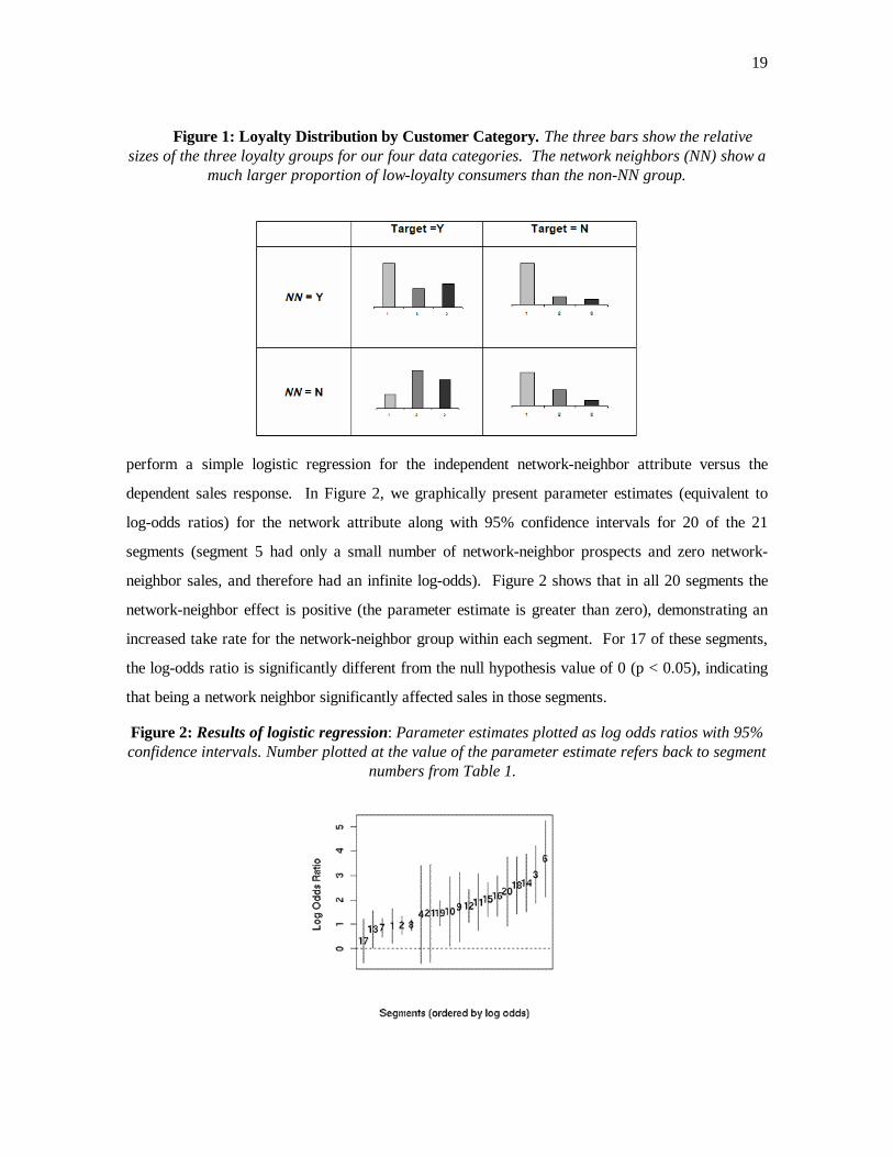
A look at the distribution of the loyalty groups across the four categories (Figure 1) of
prospects shows that the firm targeted customers in the higher loyalty groups relatively heavily. The
network-neighbor target group appears to skew toward the less loyal prospects; this is due to the fact
that Segment 22, which makes up a large part of the network-neighbor population, comprises
predominantly low-loyalty consumers.
5. ANALYSIS
Next we will show direct, statistical evidence that consumers who have communicated with prior
customers are more likely to become customers. We show this in several ways, including using our
own best efforts to build competing targeting models, and conducting thorough assessments of
predictive ability on out-of-sample data. Then we consider more sophisticated network attributes,
and show that targeting can be improved further.
5.1 Network-based marketing improves response
The segmentation provides an ideal setting to test the significance and magnitude of any
improvement in modeling by including network-neighbor information, while stratifying by many
attributes known to be important, such as loyalty and tenure. The response variable is the take rate
for the targets in the two months following the direct mailing. The take rate is the proportion of the
targets who adopted the service within a specified period following the offer. For each segment, we
19
Figure 1: Loyalty Distribution by Customer Category. The three bars show the relative sizes of the three loyalty groups for our four data categories. The network neighbors (NN) show a
much larger proportion of low-loyalty consumers than the non-NN group.
perform a simple logistic regression for the independent network-neighbor attribute versus the
dependent sales response. In Figure 2, we graphically present parameter estimates (equivalent to
log-odds ratios) for the network attribute along with 95% confidence intervals for 20 of the 21
segments (segment 5 had only a small number of network-neighbor prospects and zero network-
neighbor sales, and therefore had an infinite log-odds). Figure 2 shows that in all 20 segments the
network-neighbor effect is positive (the parameter estimate is greater than zero), demonstrating an
increased take rate for the network-neighbor group within each segment. For 17 of these segments,
the log-odds ratio is significantly different from the null hypothesis value of 0 (p < 0.05), indicating
that being a network neighbor significantly affected sales in those segments.
Figure 2: Results of logistic regression: Parameter estimates plotted as log odds ratios with 95% confidence intervals. Number plotted at the value of the parameter estimate refers back to segment
numbers from Table 1.

20
Figure 3: Take Rates for Marketing segments. Left: for each segment, comparison of the take rate of the non-network neighbors with that of the network neighbors. Size of the glyph is
proportional to the log size of the segment. There is one outlier not plotted, with a take rate of 11% for the network neighbors and 0.3% for the non-network neighbors. Reference lines are
plotted at x=y and at the overall take-rate ratio of 3.4. Right: Plot of take rate for the non-network group vs. lift ratio for the network neighbors.
While odds ratios allow for tests of significance of an independent variable, they are not as
directly interpretable as comparisons of take rates of the network-neighbor and non-network-
neighbor groups in a given segment. The take rates for the network-neighbors are plotted vs. the
non-network neighbors in Figure 3, with the size of the point proportional to the log size of the
segment. All segments have higher take rates in the network-neighbor subgroup, except for the one
segment that had no network-neighbor sales (the smallest sample size). Over the entire data set, the
network-neighbors’ take rates were greater by a factor of 3.4. This value is plotted in Figure 3 as a
dotted line with slope = 3.4. The right-hand plot of Figure 3 shows the relationship between each
segment’s take rate and its lift ratio, defined as the take rate for NN divided by the take rate for non-
NN. The plot shows that the benefit of being a network neighbor is greater for those segments with
lower overall take rates.
As Figure 3 shows, some of the segments had much higher take rates than others. In order to
assess statistical significance of the network-neighbor effect after accounting for this segment effect,
we ran a logistic regression across all segments, including main effects for the network-neighbor
attribute, dummy attributes for each segment and for the interaction terms between the two. Two of
the interaction terms had to be deleted, one from Segment 22, which only had network-neighbor

21
Table 3: Coefficients and Confidence Intervals for Final Segment Model. Significance of the attributes in the logistic regression model is shown at the .05 (*) and .01 (**) level.
cases, and one from the segment with no sales from the network neighbors. We ran a full logistic
regression, and used stepwise variable selection.
The results of the logistic regression reiterate the significance of being a network neighbor.
The final model can be found in Table 3. The coefficient of 2.0 for the network-neighbor attribute in
the final model is an estimate of the log-odds, which we exponentiate to get an odds ratio of 7.49,
with a 95% confidence interval of (5.64, 9.94). More than half of the segment effects and most of
the interactions between the network neighbor attribute and those segment effects are significant.
The interpretation of these interactions is important. Note that the magnitudes of the interaction
coefficients are negative, and very close in magnitude to the coefficients of the main effects of the

22
Table 4: Analysis of Deviance table for the network-neighbor study. Significance of the group of attributes at each step is shown at the .05 (*) and .01 (**) levels.
segments themselves. Therefore, although the segments themselves are significant, in the presence of
the network attribute the segments’ effect is mostly negated by the interaction effect. Since the
segments represent known important attributes like loyalty, tenure, and demographics, this is
evidence that being a network neighbor is at least as important in this context.
In Table 4 we present an analysis of deviance table, an analog to analysis of variance used for
nested logistic regressions (McCullagh and Nelder 1983). The table confirms the significance of the
main effects and of the interactions. Each level of the nested model is significant when using a chi-
squared approximation for the differences of the deviances. The fact that so many interactions are
significant demonstrates that the network-neighbor effect varies for different segments of the
prospect population.
5.2 Segment 22
The segment data enables us to compare take rates of network and non-network targets for the
segments that contained both types of targets. However, many of the network-neighbor targets fall
into the network-only segment 22. Segment 22 comprises prospects that the original marketing
models deemed not to be good candidates for targeting. As we can see from the distribution in
Figure 1, this segment for the most part contains consumers that had no prior relationship with the
firm.
We compare the take rates for Segment 22 with the take rates for the combined group including
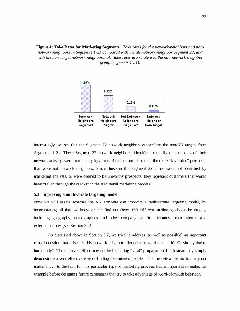
all of Segments 1-21 in the leftmost three bars of Figure 4. The network neighbor Segment 22 is
(not surprisingly) not as successful as the NN groups in Segment 1-21, since the targets in Segments
1-21 were selected based on characteristics that made them favorable for marketing. Also
23
Figure 4: Take Rates for Marketing Segments. Take rates for the network-neighbors and non-network-neighbors in Segments 1-21 compared with the all-network-neighbor Segment 22, and with the non-target network-neighbors. All take rates are relative to the non-network-neighbor
group (segments 1-21).
interestingly, we see that the Segment 22 network neighbors outperform the non-NN targets from
Segments 1-21. These Segment 22 network neighbors, identified primarily on the basis of their
network activity, were more likely by almost 3 to 1 to purchase than the more “favorable” prospects
that were not network neighbors. Since those in the Segment 22 either were not identified by
marketing analysts, or were deemed to be unworthy prospects, they represent customers that would
have “fallen through the cracks” in the traditional marketing process.
5.3 Improving a multivariate targeting model
Now we will assess whether the NN attribute can improve a multivariate targeting model, by
incorporating all that we know or can find out (over 150 different attributes) about the targets,
including geography, demographics and other company-specific attributes, from internal and
external sources (see Section 3.2).
As discussed above in Section 3.7, we tried to address (as well as possible) an important
causal question that arises: is this network-neighbor effect due to word-of-mouth? Or simply due to
homophily? The observed effect may not be indicating “viral” propagation, but instead may simply
demonstrate a very effective way of finding like-minded people. This theoretical distinction may not
matter much to the firm for this particular type of marketing process, but is important to make, for
example before designing future campaigns that try to take advantage of word-of-mouth behavior.

24
Table 5: Results of multivariate model. Significant attributes from logistic regressions across loyalty levels (p<0.05). Bold indicates significance at 0.01 level, (-) indicates the effect of the
variable was negative. (I) indicates a significant interaction with the NN variable.
Although we cannot control for unobserved similarities, we can be as careful as possible in
our analysis to ensure that the statistical profile of the NN prospects is the same as the profile for the
non-NN cases. Since our data set contains many more non-NN cases than NN cases, we match each
NN case with a single non-NN case that is as close as possible to it, by calculating propensity scores
using all of the explanatory attributes considered (as described in section 3.7). At the end of this
matching process, the NN group is as close as is reasonably possible in statistical properties to the
non-NN group.
Due to heterogeneity of data sources across the 3 loyalty groups, using the propensity scores we
created a matched data set for each group. For each (individually), we fit a full logistic regression
including interactions and selected a final model using stepwise variable selection. All attributes
were checked for outliers, transformations, and collinearity with other attributes, and we removed or
combined the attributes that accounted for any significant correlations.
Table 5 shows the results of the logistic regressions, showing the attributes that were found to
be significant, those that were negatively correlated with take rate, and those that had interactions
with the NN attribute. Each of the three models found the network-neighbor attribute to be
significant along with several others. The significant attributes tended to be attributes regarding the
prospects’ previous relationships with the firm, such as previous international services, tenure with

25
firm, churn identifiers and revenue spent with the firm. These attributes are typically correlated with
demographic attributes, which explains the lack of significance of many of the demographic
attributes considered. Interestingly, “Tenure with Firm” is significant in loyalty groups 1 and 2, but
with different signs. In the most-loyal group, tenure is negatively correlated, but in the mid-level
loyalty group it is positive. This unexpected result may be due to differing compositions of the two
groups; those with long tenure in the most-loyal group might be people who just never change
services, while long tenure in the other group might be an indicator that they are gaining more trust
in the company. In loyalty group 1, there is limited information about previous services with the
firm. For those customers, knowing whether or not the customer has responded to any previous
marketing campaigns has a significant effect.
Table 5 also shows parameter estimates for NN, and the take rates in the three loyalty groups.
The take rates are highest in the group with the most loyalty, but interestingly this group gets the
least lift (smallest parameter estimate) from the NN attribute. So, the impact of network-neighbor is
stronger for those market segments with low loyalty, where actual take rates are weakest.
5.4 Consumers not targeted
As discussed above, only a select subset of our network neighbor list was marketed to, based on
relaxed thresholds on eligibility criteria. The remainder of the list, the non-target network
neighbors, made up the majority. They were omitted for various reasons: they were not believed to
have high-tech capacity; they were on a do-not-contact list; address information was unreliable, etc.
Nonetheless, we were able to identify whether they purchased the product in the follow-up time
period. The take rate for this group was 0.11%, and is shown relative to the target groups as the
right-most bar in Figure 4. Although they were not even marketed to, their take rate is almost half
that for the non-NN targets—chosen as some of the best prospects by the marketing team. This
group comprises consumers without any known favorable characteristics that would have put them
on the list of prospects. The fact that they are network neighbors alone supports a relatively high
take rate, even in the absence of direct marketing. This lends some support to an explanation of
word-of-mouth propagation rather than homophily.
Finally, we will briefly discuss the remainder of the consumer space, the non-NN non-target
group. Unfortunately, it is very difficult to estimate a take rate in this category, which could be
considered a baseline rate for all of the other take rates. To do this, we would need to estimate the

26
size of the space of all prospects. This includes all of the prospects the firm knows about, as well as
those customers of the firm’s competitors, and consumers who might purchase this product that do
not have current telecommunications service with any provider. It has been established that the size
of the communications market is difficult to estimate (Poole 2004); our best estimates of this
baseline take rate put it at well below 0.01%, at least an order of magnitude less than even the non-
target network-neighbors.
On the other hand, a by-product of our study is that we can upper-bound the effect of the mass
marketing campaigns in general, by comparing the target-NN group and the non-target-NN group.
The difference in take rates between the targeted network neighbors and the not-targeted network
neighbors is about 10 to 1. This difference cannot all be attributed to the marketing effect, since the
targeted group was specifically chosen to be better prospects, and it is likely that more of them
would have signed up for the service even in the total absence of marketing. But it does seem
reasonable to call this factor of 10 an upper bound on the effect of the marketing.
5.5 Out-of-sample ranking performance
These results suggest that we can give fine-grained estimations as to which customers are more
or less likely to respond to an offer. Such estimations can be quite valuable: the consumer pool is
immense, and a campaign will have a limited budget. Therefore, being able to pick a better list of
“top-k” prospects will lead directly to increased profit (assuming targeting costs are not much higher
for higher-ranked prospects). In this section, we show that combining the network-neighbor attribute
with the traditional attributes improves the ability to rank customers accurately.
For each consumer, we create a record comprising all of the traditional attributes, including loyalty,
demographic, and geographic attributes, as well as network-neighbor status. Note that in different
business scenarios, different types and amounts of data are available. For example, for low-loyalty
customers very few descriptive attributes are known. We report results here using all attributes; the
findings are qualitatively similar for every different subset of attributes we have tried (viz., segment,
loyalty, geography, demographic). The response variable is the same as above, and we used the
same logistic regression models. We measure the predictive ranking ability in the binary response
variable by an increase in the Wilcoxon-Mann-Whitney statistic, equivalent to the area under the
ROC curve (AUC). Specifically, the AUC is the probability that a randomly chosen (as-

27
Table 6. ROC Analysis. AUC values resulting from the application of logistic regression models built using all available attributes with (trad atts + NN) and without (trad atts) the network-
neighbor attribute We see an increase in AUC across all loyalty groups when the NN attribute is included in the model.
Figure 5a) Lift curves. Power of segmentation curves for models built with all attributes, with (trad atts) and without (trad atts + NN). The model with the NN attribute outperforms the model without it. For example, if the firm sent out 50% of the mailers, they would get 70% of the positive responses with the NN compared to only receiving 63% of the responses without it.
Figure 5b) Top-k analysis. Consumers are ranked by the probability scores from the logistic regression model. The model including the NN attribute outperforms the model without. For example, for the top-20% of targets, the take rate is 1.51% without the NN attribute and 1.72% with the NN attribute.
of-yet-unseen) taker will be ranked higher than a randomly chosen non-taker; AUC=1.0 means the
classes are perfectly separated, and AUC=0.5 means the list is randomly shuffled. All reported AUC
values are averages obtained using 10-fold cross-validation.
Table 6 shows the AUC values for the three loyalty groups, quantifying the expected benefit
from the improved logistic regression models. There is an increase in AUC for each group, with the
largest increase belonging to loyalty level 1, for which the least information is available—note that
here the ranking ability without the network information is not much better than random.
To visualize this improvement, Figure 5a shows cumulative response (“lift”) curves when using
the model on loyalty group 3. The lower curve depicts the performance of the model using all

28
traditional attributes, and the upper curve includes the traditional marketing attributes and the
network-neighbor attribute. In Figure 5b, one can see the marked improvement that would be
obtained from sending to the top-k prospects on the list. For example, for the top-20% of the list,
without the NN attribute, the take rate is 1.51%; with the NN attribute, it is 1.72%. The NN
attribute does not improve the ranking for the top-10% of the list.
5.6 Improving performance by adding more sophisticated network attributes
Knowing whether a consumer is a network neighbor is one of the simplest indicators of consumer-to-
consumer interaction that can be extracted from the network data. We now investigate whether
augmenting the model with more sophisticated social-network information can add additional value.
In this section, we focus on the social network comprising (only) the current customers of this
service (which here we will call “the network”), along with the periphery of prospects who have
communicated with those on the network (the network neighbors). We investigate whether we can
improve targeting by using more sophisticated measures of social relationship with the network of
existing customers.
Table 7 summarizes a set of additional social-network attributes that we add to the logistic
regression. The terminology we use is borrowed to some degree from the fields of social network
analysis and graph theory. Social network analysis (SNA) involves measuring relationships
(including information transmission) between people on a network. The nodes in the network
represent people and the links between them represent relationships between the nodes. SNA
measures help quantify intuitive social notions, such as connectedness, influence, centrality, social
importance, and so on. Graph theory helps to understand problems better by representing them as
interconnected nodes, and provides vocabulary and methods for operating mathematically.
Three of the attributes that we introduce can be derived from a prospect’s local neighborhood
(the set of immediate communication partners on the network; recall that these all are current
customers). Degree measures the number of direct connections a node has. Within the local
neighborhood, we also count the number of Transactions, and length of those transactions (Seconds
of Communication).
The network is made up of many disjoint subgraphs. Given a graph G = (V,E), where V is a set
of vertices (nodes) and E is a set of links between them, the connected components of G are the sets
of vertices such that all vertices in each set are mutually connected (reachable by some path), and no

29
Table 7: Network attribute descriptions.
two vertices in different sets are connected. The size of the connected component may be an
indicator for awareness of and positive views about the product. If a prospect is linked to a large set
of “friends” all of whom have adopted the service, she may be more likely to adopt herself.
Connected Component Size is the size of the largest connected component (in the network) to
which the prospect is connected.
We also move beyond a prospect’s local neighborhood. Observing the local neighborhoods of a
prospect’s local neighbors, we can define a measure of social similarity. We define social similarity
as the size of the overlap in the immediate network neighborhoods of two consumers. Max
Similarity is the maximum social similarity between the prospect and any neighbors of the prospect.
Finally, the firm also can observe the prior dynamics of its customers. In particular, the firm can
observe which customers communicated before and/or after their adoption as well as the date
customers signed up. Using this information, we define influencers as those subscribers who signed
up for the service, and subsequently we see one of their network neighbors sign up for the service.
Connected to Influencer is an indicator of whether the prospect is connected to one of these
influencers. We appreciate that we do not actually know if there was true influence.
We use all of the aforementioned attributes, and show AUC values for these predictive models
in Table 8. We find that some of these network attributes have considerable predictive power
individually, and have even more value when combined. This is indicated by AUCs of .68 for both
Transactions and Seconds of Communication. We do not find high AUCs individually for
Connected Component Size, Similarity, or Connected to Influencer. Ultimately, we find that the
logistic regression model built with the network attributes results in an AUC of 0.71 compared to an

30
Figure 6a) Lift curves. Power of segmentation curves for models built with all traditional attributes, with (trad atts + net) and without (trad atts) the network attributes. If the firm sent out 50% of the mailers, they would have received 77% of the positive responses with the network attributes compared to receiving 63% of the responses without the network attributes.
Figure 6b) Top-k analysis. The model including the network attributes (trad atts + net) outperforms the model without them (trad atts). For example, for the top 20% of target ranked by score, the take rate is 2.2% without the network attributes and 3.1% with the network attributes.
Table 8. ROC Analysis. AUC Values resulting from logistic regression models built on each of the constructed network attributes individually. Results are presented for loyalty level 3
customers.

31
AUC of 0.66 without the network attributes—using only the traditional marketing attributes
described in previous sections. (Recall that this represents the ability to rank the network neighbors,
who have especially high take rates as a group, as we already have shown.)
Interestingly, when we combine the traditional attributes with the network attributes, there is no
additional gain in AUC, even though many of these attributes were shown to be significant in the
broader analysis above. The similarities represented implicitly or explicitly in the network attributes
seem to account for all useful information captured by traditional demographics and other marketing
attributes. Traditional demographics and other marketing attributes not adding value is not only of
theoretical interest, but practical as well—for example, in cases such as this where demographic data
must be purchased.
Our result is further confirmed by the lift and take rate curves displayed in Figure 6a and
Figure 6b respectively. One can achieve substantially higher take rates using the new network
attributes, than using the traditional attributes. For example, we find that for the top-20% of the
targeted list, without the network attributes, the take rate is 2.2%; with the network attributes, it is
3.1%. Likewise, at the top-10% of the list the take rate with the network attributes is 4.4%
compared to 2.9% without them.
6. LIMITATIONS
We believe our study to be the first to combine data on direct customer communication with
data on product adoption in order to show the effect of network-based marketing statistically.
However, there are limitations in our study that are important to point out.
There are several types of missing, incomplete, or unreliable data which could influence our
results. We have records of all of the communication to and from current customers of the service.
That is not true for all the network-neighbor consumers. As such, we do not have complete
information about the network-neighbor targets (as well as the non-network-neighbor targets). In
addition, some of the attributes we used were collected by purchasing data from external sources.
These data are known to be at least partially erroneous and outdated, although it is not well known
how much so. An additional problem is joining data on customers from the external sources to
internal communication data, leading to missing data or sometimes just blatantly incorrect data.
Finally, telecommunications firms are not legally able to collect information regarding the actual
content of the communication, so we are not able to determine if the consumers in question discussed

32
the product. In this regard, our data is inferior to some other domains where content is visible, such
as Internet bulletin boards, or product discussion forums.
We expect the network-neighbor effect to manifest itself differently for different types of
products. Most of the studies done to date on “viral marketing” have focused on the types of
products that people are likely to talk about, such as a new, high-tech gadget or a recently released
movie. We expect there to be less buzz for less “sexy” products, like a new deodorant, or a sale on
grapes at the supermarket. The study presented in this paper involves a new telecommunications
service, which involves a new technology and features that consumers have perhaps never been
exposed to before. The firm hopes the new technology and features are such that they would
encourage word of mouth. But what can we say about other products that might not be quite so
buzz-worthy?
In order to study this, we compared the new service studied here to a rollout of another product
by the same firm. This other "product" was simply a new pricing plan for an older
telecommunications service. Customers who signed up for this new plan could stand to save a
significant amount of money, depending on their current usage patterns. However, the range and
variety of telecommunications pricing plans in the marketplace is so extensive, and so confusing to
the typical consumer, that we do not believe that this is the type of product that would generate a lot
of discussion between consumers. We refer to the two products as the "pricing plan" and the "new
technology." For the pricing plan, we have the same knowledge of the network as we do for the new
technology. For those consumers that belong to the pricing plan, we know whom they communicate
with, and then we can follow these network-neighbor candidates to see if they ultimately sign up for
the plan. We construct a measure of "network-neighborness" as follows. For a series of consecutive
months, we gather data for all customers who ordered the product in that month. We calculate the
percentage of these new customers that were network-neighbors, i.e., those who had previously
communicated with a user of the product. This percentage is a measurement of the proportion of
new sales being driven by network effects. By comparing this percentage across two products, we
get insight into which product stimulates network effects more.
We now look at this value for our two products over an eight-month period. The time period
for the two products was chosen so that it would be within the first year after the product was
broadly available. The results are shown in Figure 7. The two main points to take away are that
the new service has a higher percent of purchasers that are network-neighbors, and also an

33
increasing one (except for the dip in month 5). In contrast the pricing plan has a flat network-
neighbor percentage, never increasing above 3%.
Interestingly, the dip in the plot for the new service corresponds exactly to the month of the
direct marketing discussed earlier. Before the campaign, we can see that the network-neighbor effect
was increasing, that more and more of the purchasers in a given month were network neighbors.
During the mass marketing campaign, we exposed many non-network-neighbors to the service, and
many of them ended up purchasing it, temporarily dropping the network-neighbor percent. After the
campaign, we see the network-neighbor percent starting to increase again.
This network-neighborness measure should not be confused with the success of the product, as
the pricing plan was quite successful from a sales perspective. But it does suggest that the pricing
plan is a product that has less of a network-based spread of information. This difference might be
due to the new service creating more word-of-mouth, or perhaps we are seeing the effects of
homophily.
Figure 7: Network-neighborness Plot for New Service vs. Pricing Plan.
People who interact with each other are more likely to be similar in their propensity for purchasing
the new service, than in their propensity for purchasing a particular pricing plan. Again, the effects
of word-of-mouth vs. homophily are difficult to discern without knowing the content of the
communication.
7. DISCUSSION
One of the main concerns for any firm is when, how and to whom they should market their
products. Firms make marketing decisions based on how much they know about their customers and
potential customers. They may choose to mass market when they do not know much. With more

34
information, they may market directly based on some observed characteristics. We provide strong
evidence that whether and how well a consumer is linked to existing customers is a powerful
characteristic on which to base direct marketing decisions. Our results indicate that a firm can
benefit from the use of social networks to predict the likelihood of purchasing. Taking the network
data into account improves significantly and substantially over both the firm’s own marketing “best
practices,” and our best efforts to collect and model with traditional data.
The sort of directed network-based marketing that we study here has applicability beyond
traditional telecommunciations companies. For example, Ebay recently purchased internet-telephony
upstart Skype for $2.6 billion; they now also will have large-scale, explicit data on who talks to
whom. With gmail, Google’s email service, Google now has access to explicit networks of consumer
interrelationships, and already is using gmail for marketing; directed network-based marketing might
be a next step. Various systems have emerged recently that provide explicit linkages between
acquaintances (e.g., MySpace, Friendster, Facebook), which could be fruitful fields for network-
based marketing. As more consumers create interlinked blogs, another data source arises. More
generally, these results suggest that such linkage data potentially could be a sort of data considered
for acquisition by many types of firms, as purchase data now is being collected routinely by many
types of retail firms through loyalty cards. Even academic departments could benefit from such
data; for example, the enrollment in specialized classes could be bolstered by "marketing" to those
linked to existing students. Such links exist (e.g., via email). It remains to design tactics for using
them that are acceptable to all.
It is tempting to argue that we have shown that customers discuss the product, and that
discussion helps to improve take rates. However, word of mouth is not the only possible explanation
for our result. As discussed in detail above, it may be that the network is a powerful source of
information on consumer homophily, which is in accord with social theories (Blau 1977; McPherson,
Smith-Lovin et al. 2001). We have tried to control for homophily, by using a propensity-matched
sample to produce our logistic regression model. However, it may well be that direct
communications between people is a better indicator of deep similarity than any demographic or
geographic attributes. Either cause, homophily or word-of-mouth, is interesting both theoretically
and practically.

35
8. ACKNOWLEDGEMENTS
We would like to thank DeDe Paul and Deepak Agarwal of AT&T, as well as Chris Dellarocas
of the University of Maryland for useful discussions and helpful suggestions. We would also like to
thank the three anonymous reviewers that offered insightful comments on previous drafts.
9. REFERENCES
Adomavicius, G. and A. Tuzhilin (2005). "Toward the next generation of recommender systems: A
survey of the state-of-the-art and possible extensions." IEEE Transactions on Knowledge
and Data Engineering 17(6): 734-749.
Agarwal, D. and D. Pregibon (2004). Enhancing communities of interest using Bayesian stochastic
blockmodels. In the Proc. of the 4th SIAM Intl. Conf. on Data Mining, Lake Buena Vista,
Florida.
Bass, F. M. (1969). "New product growth for model consumer durables." Management Science
15(5): 215-227.
Blau, P. M. (1977). Inequality and heterogeneity: A primitive theory of social structure. New York,
Free Press.
Bowman, D. and D. Narayandas (2001). "Managing customer-initiated contacts with manufacturers:
The impact on share of category requirements and word-of-mouth behavior." Journal of
Marketing Research 38: 291–297.
Brin, S. and L. Page (1998). The anatomy of a large-scale hypertextual web search engine. In the
Proc. of the 7th Intl. Conf. on World Wide Web, Brisbane, Australia.
Case, A. C. (1991). "Spatial Patterns in Household Demand." Econometrica 59(4): 953-965.
Chan, P. and S. Stolfo (1998). Toward scalable learning with non-uniform class and cost
distributions: A case study in credit card fraud detection. In the Proc. of the 4th Intl. Conf.
Knowledge Discovery and Data Mining, New York, NY.
Clearwater, S. H. and E. G. Stern (1991). "A rule-learning program in high energy physics event
classification." Computer Physics Communications 67(2): 159-182.
Dellarocas, C. (2003). "The digitization of word of mouth: Promise and challenges of online
feedback mechanisms." Management Science 49(10): 1407-1424.
Domingos, P. and M. Richardson (2001). Mining the network value of customers. In the Proc. of the
7th Intl. Conf. on Knowledge Discovery and Data Mining, San Francisco, CA, ACM Press.

36
DuMouchel, W., C. Volinsky, et al. (1999). Squashing flat files flatter. In the Proc. of the 5th Intl.
Conf. on Knowledge Discovery and Data Mining",.
Fichman, R. G. (2004). "Going beyond the dominant paradigm for IT innovation research: Emerging
concepts and methods." Journal of the Association for Information Systems 5(8): 314-355.
Fildes, R. (2003). "New-product diffusion models." International Journal of Forecasting 19(2): 327-
328.
Frenzen, J. and K. Nakamoto (1993). "Structure, cooperating, and the flow of market information."
Journal of Consumer Research 20(December): 360-365.
Getoor, L. (2005). Tutorial on statistical relational learning. 15th Intl. Conf. on Inductive Logic
Programming 2005, Bonn, Germany.
Getoor, L., N. Friedman, et al. (2001). Learning probabilistic relational models. Relational Data
Mining. S. Dzeroski and N. Lavrac, Springer-Verlag.
Getoor, L., N. Friedman, et al. (2002). "Learning probabilistic models of link structure." Journal of
Machine Learning Research 3(December): 679-707.
Gladwell, M. (1997). The coolhunt new yorker. The New Yorker: 78-88.
Gladwell, M. (2002). The tipping point: How little things can make a big difference, Boston, Back
Bay Books.
Hightower, R., M. K. Brady, et al. (2002). "Investigating the role of the physical environment in
hedonic service consumption: an exploratory study of sporting events." Journal of Business
Research 55(9): 697-707.
Hoff, P. D., A. E. Raftery, et al. (2002). "Latent space approaches to social network analysis."
Journal of the American Statistical Association 97(460): 1090-1098.
Huang, Z., W. Chung, et al. (2004). "A graph model for e-commerce recommender systems."
Journal of the American Society for Information Science and Technology 55(3): 259-274.
Japkowicz, N. and S. Stephen (2002). "The class imbalance problem: A systematic study "
Intelligent Data Analysis 6(5): 429-450.
Joshi, M., V. Kumar, et al. (2001 ). Evaluating boosting algorithms to classify rare classes:
Comparison and improvements. In the Proc. of the 1st IEEE Intl. Conf. on Data Mining,
San Jose, CA.
Kautz, H., B. Selman, et al. (1997). "Referral web: Combining social networks and collaborative
filtering." Communications of the ACM 40(3): 63-65.

37
Kleinberg, J. (1999). "Authoritative sources in a hyperlinked environment " Journal of the ACM
46(5): 604-632.
Kumar, V. and T. V. Krishnan (2002). "Multinational diffusion models: An alternative framework."
Marketing Science 21(3): 318-330.
Liben-Nowell, D. and J. Kleinberg (2003). The link prediction problem for social networks. In the
Proc. of the 12th Intl. Conf. on Information and Knowledge Management, ACM Press.
Linden, G., B. Smith, et al. (2003). "Amazon.com recommendation - Item-to-item collaborative
filtering." Ieee Internet Computing 7(1): 76-80.
Macskassy, S. and F. Provost (2004). Classification in Networked Data: A toolkit and a univariate
case study. CeDER Working Paper #CeDER-04-08, Stern School of Business, New York
University, NY, NY.
Mahajan, V., E. Muller, et al. (1984). "Introduction strategy for new products with positive and
negative word-of-mouth." Management Science 30(12): 1389-1404.
McCullagh, P. and J. A. Nelder (1983). Generalized linear models. London ; New York, Chapman
and Hall.
McPherson, M., L. Smith-Lovin, et al. (2001). "Birds of a feather: Homophily in social networks."
Annual Review of Sociology 27: 415-444.
Mease, D., A. Wyner, et al. (2004). "Boosted classification trees and class probability/quantile
estimation." Journal of Machine Learning Research (submitted).
Montgomery, A. L. (2001). "Applying quantitative marketing techniques to the Internet." Interfaces
31(2): 90-108.
Newton, J. and R. Greiner (2004). Hierarchical probabilistic relational models for collaborative
filtering. Statistical Relational Learnng Workshop at the 21st Intl. Conf. on Machine
Learning, Alberta, Canada.
Paumgarten, N. (2003). No. 1 fan dept. acknowledged. The New Yorker. 2003-05-05.
Perlich, C. and F. Provost (2006). "ACORA: Distribution-based Aggregation for Relational
Learning from Identifier Attributes." Machine Learning Journal 62 (1/2): 65-105.
Poole, D. J. (2004). Estimating the size of the telephone universe. In the Proc. of the 10th ACM
SIGKDD Intl. Conf. on Knowledge Discovery and Data Mining Seattle, WA, ACM.

38
Richardson, M. and P. Domingos (2002). Mining knowledge-sharing sites for viral marketing. In the
Proc. of the 8th Intl. Conf. on Knowledge Discovery and Data Mining, Edmonton, Canada,
ACM.
Rogers, E. M. (2003). Diffusion of innovations. New York, Free Press.
Rosenbaum, P. R. and D. B. Rubin (1984). "Reducing bias in observational studies using
subclassification on the propensity score." Journal of the American Statistical Association
79: 516-524.
Tout, K., D. J. Evans, et al. (2005). "Collaborative filtering: Special case in predictive analysis."
International Journal of Computer Mathematics 82(1): 1-11.
Ueda, T. (1990). "A Study of a Competitive Bass Model Which Takes into Account Competition
among Firms." Journal of the Operations Research Society of Japan 33(4): 319-334.
Van den Bulte, C. and G. L. Lilien (2001). "Medical innovation revisited: Social contagion versus
marketing effort." American Journal of Sociology 106 (5): 1409-35.
Walker, R. (2004). The hidden (In plain site) persuaders. New York Times Magazine: 69-75,104.
Weiss, G. and F. Provost (2003). "Learning when training data are costly: The effect of class
distribution on tree induction." Journal of Artificial Intelligence Research 19: 315-354.
Weiss, G. M. (2004). "Mining with rarity: A unifying framework." SIGKDD Explorations 6(1): 7-
19.
Yang, S. and G. M. Allenby (2003). "Modeling Interdependent Consumer Preferences." Journal of
Marketing Research 40(3): 282-294