1

NETWORK ANALYSIS OF A BENTHIC FOOD WEB MODEL OF A PARTLY RECLAIMED ISLAND IN THE SUNDARBAN MANGROVE ECOSYSTEM, INDIA

SANTANU RAY1, ROBERT E. ULANOWICZ2, N. C. MAJEE3 and A. B. ROY3

1Biomathematical Laboratory, Czech Academy of Sciences and University of South Bohemia, 31 Branisovska, 37005 Ceske Budejovice, Czech Republic

2University of Maryland System, Chesapeake Biological Laboratory, Solomons, MD 20688-0038, USA

3Department of Mathematics, Jadavpur University, Calcutta 700 032, INDIA

ABSTRACT

Network analysis is performed on a 14 species food web model of the ecosystem occupying a mudflat on a partly

reclaimed island of the Sundarban mangrove ecosystem. The results demonstrate a dramatic difference between this

heavily impacted mangrove ecosystem in its modes of primary and secondary production and its diminished role of

detritus vis-a-vis its less disturbed counterparts.

Unlike most benthic mangrove systems, the Sundarban bottom community receives a large contribution from the

phytoplankton populations. In this system herbivory and detritivory are virtually equal, in contrast to the usual

herbivory:detritivory ratio of 1:5. Anthropogenic impacts have changed the physiography of this system so as to

increase the relative importance of zooplankton and meiobenthos as herbivores. Although a slight degree of

omnivory is exhibited by the populations of larger organisms, all flows of each integer of trophic length into a food

chain may be aggregated that represents the underlying trophic status of the starting food web. Only a small number

of pathways of recycle can be identified (31), and the Finn cycling index for this system is quite low (8.4%).

Litterfall comprises only 16% of the total system input, which is very little in comparison with most mangrove

systems. Pathway redundancy is rather high in this ecosystem, indicating that the surviving system is probably

highly resilient to further perturbations, as one might expect for a highly impacted system.

Keywords: Network analysis, benthic, foodweb, mangrove, and ascendancy

-------------------------------------------------------------------------------------------------------------------------------------------------------------------------------------------------------

1Corresponding author, e-mail: sray@entu.cas.cz

2

1.Introduction

The Gangetic delta of the Hooghly-Brahamaputra estuarine complex, by dint of its exciting mangrove ecosystem,

has achieved a notable place on the global map. This complex is approximately 170 km in length and at some places

exceeds 60 km in width, making it the greatest halophytic formation in the world. It extends over two countries:

India (West Bengal) and Bangladesh. The entire region is divided by a dense network of rivers, canals and creeks.

The mangrove forest, comprising 4200 sq. km. [3], is called “Sundarban” – a name thought to be derived either from

beautiful forest (Bengal: “Sundara” = beautiful) or from forest of “Sundari” (local name of Heritiera fomes). In

addition to sheltering some of the worlds, most graceful game, the ecosystem also supports a luxuriant flora and

fauna: plankton, nekton, benthos, salt marshes, in sand and mud flats. The mangrove system covers several islands,

some of which are partly developed but most of which remain virgin. Sagar Island, particularly reclaimed and the

largest island in this deltaic complex and is cris-crossed by twelve tidal creeks of various sizes, fringed with

mangrove vegetation, and all connected with the principal estuarine water.

Below we consider a 14 species network of trophic exchanges in the ecosystem of the mud flats on Sagar Island.

Earlier, the structure and function of this ecosystem particularly the virgin parts were investigated using

deterministic models [15,17,18,23] and disturbed part also studied by some authors [9,21]. The two or three species

models these investigators employed were unable to afford them a full understanding of this system. Here, we use

network analysis to give further insight into this mangrove ecosystem, which has been reclaimed in places, but over

all is gradually diminishing.

Network analysis has been used to quantify the structure of system networks, the degree of cycling, and the

magnitudes of interdependency among components [1,8,10,32.35]. We employ it here to calculate the number of

trophic levels, the underlying trophic dynamics, the degree of trophic specialization, the relative dependence of each

compartment on a range of energy sources, the effective trophic position of each component, the interdependency

among compartments, the overall system ascendancy and the redundancy (see below.)

The data used in this model were collected from different sources, including direct field observation by one of the

authors (SR), from various Ph.D. theses project reports [1,4,6,7,19,22,33]. In most cases the organisms were

sampled fortnightly at different stations. Gross primary productivity (for phytoplankton) was estimated using “light

3

and dark bottle method” of Strickland [26] and Strickland and Parson [27]. Biomasses are initially measured as dry

weight: A known number of animals/plants were dried until their weight becomes constant. The energy content of

the material was determined by “bomb calorimetry”. Feeding rates were measured using the radiometric technique

of Moore et al. [16] and also by gravimetric methods [14]. Respirational and metabolic losses were assessed by

keeping the animal enclosed in a limited volume of water cut off from the atmosphere [34]. In some cases it was

difficult to determine the rate of respiration in the field, but values for ingestion, consumption, egestion and

excretion were available, so that respiration could be determined by difference. All values for the flows of energy

were converted into kcal m-2 y-1 [24], and the standing stocks were reported as kcal m-2.

2. Quantitative Methods

The computer package NETWRK [13] was used to perform standardized matrix manipulations that constitute the

backbone of what has come to be known as Network Analysis. There are four major tasks performed by NETWRK,

(1) The evaluation of all direct and indirect bilateral relationships in a network of trophic exchanges, (2) The

elucidation of the trophic structure immanent in the network, (3) The identification and quantification of all

pathways for recycling medium extant in the network, and (4) The quantification of the overall status of the

network’s structure.

The fundamental data used in Network Analysis are the exchanges between the system components. We begin by

denoting the magnitude of the transfer of medium from i to j as Tij, where both i and j run from 1 to n, the number of

components in the system. (To denote exogenous transfers to and from the system, one may identify 0 as the source

of external inputs and n+1 as the destination of external outputs.) The activity level of the entire network is

characterized by the sum of all Tij, and is called the total system throughput. The the crux of the calculations,

however, revolves around the accompanying matrix of dietary coefficients, G, where the matrix components are

calculated from the Tij as Gij = Tij /kTkj. In words, Gij is the fraction of j’s diet that is comprised by i. The algebraic

powers of the G matrix are extremely informative. The reader is invited to test, for example, that the i-jth element of

G2 , quantifies exactly what fraction of the input to j travels from i across all pathways of length 2. Similarly, the i-jth

element of Gm describes the fraction of all input to j that travels from i to j along all trophic pathways of length m.

4

Because G has been normalized by the total input to each column j, the elements Gij are all less than or equal to

unity. The elements of successively higher algebraic powers of G tend to diminish in magnitude. In fact, one might

question whether the infinite series of such powers (S = G0 + G1 + G2 + G3 + …) converges to any finite limit? It

may indeed be demonstrated that the series does converge to the finite limit, S = [I – G]-1, where I (= G0) is the

identity matrix with ones along the diagonal and zeroes elsewhere. The limit matrix, S, is called the “structure

matrix”, and the i-jth element represents the fraction of total input to j that flows both directly and indirectly from i

along all pathways of all lengths.

The powers of G can be used to calculate how much of what a species ingests arrives over pathways of various

integer lengths [12,20,31]. This information allows one to apportion the activity of that taxon to the successive links

of a chain of virtual integer trophic levels, or equivalent trophic chain, or trophic pyramid. The matrix created from

the powers of G that maps the food web into the virtual chain is called the Lindeman transformation matrix. The

sum of each column of this latter matrix yields a decimal figure >1 that characterizes the effective trophic level of

the corresponding taxon. Finally, Szyrmer and Ulanowicz [28] showed how best to normalize the structure matrix,

S, so that the ith element of the jth column reveals how much the jth taxon depends both directly and indirectly upon

taxon i. The normalized matrix is referred to as the total dependency matrix and its elements are sometimes referred

to as dependency coefficients. They also derived a corresponding normalization that allows one to trace the overall

contributions from any one taxon to any other in terms of a total contribution matrix.

The matrix of transfers, T, by virtue of its pattern of zero and nonzero elements, describes the network connection

topology. It is possible to perform a depth-first search on T (otherwise known as a backtracking algorithm) to

identify all the simple cycles extant in the network [29]. (Simple cycles contain no repeated taxa.) Often the pattern

of recycled flows reveals clues to how the system is functioning to process medium [2]. In any event, the fraction of

the total activity, T, comprised by the recycled flow is called the Finn Cycling Index, and has been used to gauge the

degree of maturity of some systems [11].

Finally, Ulanowicz [30] demonstrates how one may characterize both the activity level and the degree of

organization of a network by an informational index called the system ascendency. Organization is evidence of

5

constraint acting in a structure. To quantify the average degree of constraint at work in a system, one begins in

information theory by quantifying the opposite notion, the degree of indeterminacy. One estimates that the

probability that any quantum of medium leaves taxon i, as estimated by the frequency m Tim/T. According to

Boltzmann [5], the indeterminacy associated with this marginal probability is –k*log(j Tij/T), where k is a scalar

constant. In order to gauge the constraint that is necessary to guide this quantum into taxon j in particular, one

estimates the conditional probability that, having left i, the quantum arrives at j as the quotient Tij/kTkj. The

corresponding indeterminacy, -k*log(Tij/kTkj), should in most cases be less than the unconditional indeterminacy

quoted above. The difference between the apriori and aposteriori indeterminacy’s should, therefore, measure the

amount of constraint guiding the flow from i to j. This difference takes the form, k*log([Tij*T]/[mTim*kTkj]).

In order to estimate the average amount of constraint operative in the network, it is necessary simply to weight each

such i-j term by the joint probability of the i-jth flow occurring (as estimated by the frequency Tij/T) and sum over

all possible combinations of i and j. The result is what is called the average mutual information of the flow network,

AMI, and takes the explicit form, AMI = k*i,j(Tij/T)log([Tij*T]/[mTim*kTkj]). Like other informational indices,

AMI does not have physical dimensions. In order to impart physical extent to AMI, we elect to set the scalar

constant, k, equal to the total system throughput, T and call the result the system ascendency, A. It follows that A =

i,jTijlog([Tij*T]/[mTim*kTkj]).

The problem with the full ascendency often is that it is heavily dominated by the scale of system activity, T. In order

to focus on the organizational aspect of A, we note that an upper bound on A exists in the diversity of system

processes as scaled by T. This limit is called the system’s development capacity, C, where C = i,jTijlog(Tij/T).

Because the difference = C-A is always non-negative, one may speak of as the system overhead. It is usually

dominated by the redundancy of parallel pathways in the network. It follows that the organizational status of the

network is related to the fraction of the capacity that appears as constrained flow, or what is called the relative

ascendency, A/C. In similar fashion, the relative overhead becomes F/C, which is dominated by the relative

redundancy.

3. Results and Discussion

6

Experiments with various levels of aggregation culminated in the energy flow diagram are depicted (Fig. 1). Only

those individual species that are both taxonomically and functionally similar have been aggregated. There are total

of 14 compartments:

1. Benthic algae – Various algal species (viz., Ulva sp., Enteromorpha sp., Vaucheria sp., Oscillatoria sp.,

Lyngbya sp., Catenella sp., Chaetomorpha sp., and Xenococcus sp., are found on the mud surface as a green

mat, exposed during low tide, but submerged during extreme high tide.

2. Phytoplankton – Minute, photosynthetically active plants floating in the water columns, more than 30 species

are recorded.

3. Macrophytes – Mainly grasses in salt marshes, e.g., Spartina sp., Saueda sp., and Salicornia sp., and also a few

stunted Phoenix sp. are noticed.

4. Zooplankton – More than 18 species of small animal plankton are recorded

5. Browsers – Mainly mollusks (Littorina spp.), benthic amphipods, etc. are noticed

6. Deposit/filter feeders – In particular, Calms, mollusks, siphunculid and echurids, crabs (Uca spp.) etc. are

recorded

7. Meio/macro benthic herbivores – Mainly annelids (polychaetes), soil nematodes and insect larvae (Chironomid

spp.) are found

8. Bacteria – Numerous bacterial species are also recorded in the litter and detritus (bacterioplankton, where

applicable, are lumped with the phytoplankton).

9. Benthic detritivores – Including unicellular protozoa, insect larvae, nematodes, mollusks etc. are recorded

10. Pelagic detritivores – Mainly the mullet group of fishes, are recorded e.g. Partia spp.

11. Macrobenthic carnivores – Nematodes, some insect larvae (Culicoides spp.), sea anemone, holothuroids etc. are

found.

12. Pelagic carnivores – Small catfishes and other small invertebrates such as Chaetognaths sp. etc. are recorded.

13. Top carnivores – Large fish such Lates sp. etc. is noticed.

14. Detritus – The nonliving compartment is formed mostly within the food web but also with some input from

upper zone of Phoenix sp. patches.

7

We discuss first the contribution and dependency coefficients, which are tabulated (Table 1 and Table 2). Each

contribution coefficient (Table 1) represents the fraction of a particular component, throughput that is contributed to

the diet of another specific component. The results show that the phytoplankton community (compartment – 2)

makes a significant contribution to the community production of the mud flat. This result is in marked contrast to the

situation in other mudflat communities. Previously, this mud flat had been dominated by Phoenix sp. – an important

mangrove plant; but due to heavy infiltration and deforestation by humans, this species is currently faces extirpation.

Only a few patches of this plant (and in some areas, dead roots) are to be found. Once this mangrove species is

disappeared, erosion by the wave action no longer is prevented, and many ditches form in the mud flat. Most of the

time these erosions are inundated by tidal water. The relatively elevated areas are covered by benthic algae, some

grasses, and by scanty Phoenix sp. populations. Because the ditches are constantly inundated by water,

phytoplankton are more abundant in these ditches.

It was mentioned earlier how only remnants of Phoenix sp. vegetation can be found in the Sundarban. In comparison

with other mangrove species Phoenix sp. produces less litter, as its leaf fall is scant, and its leaves are small,

needle-shaped and narrow [25]. As a result, litterfall makes an unusually small contribution to the Sundarban

ecosystem in comparison to other mangrove ecosystems, which are usually dominated by this input.

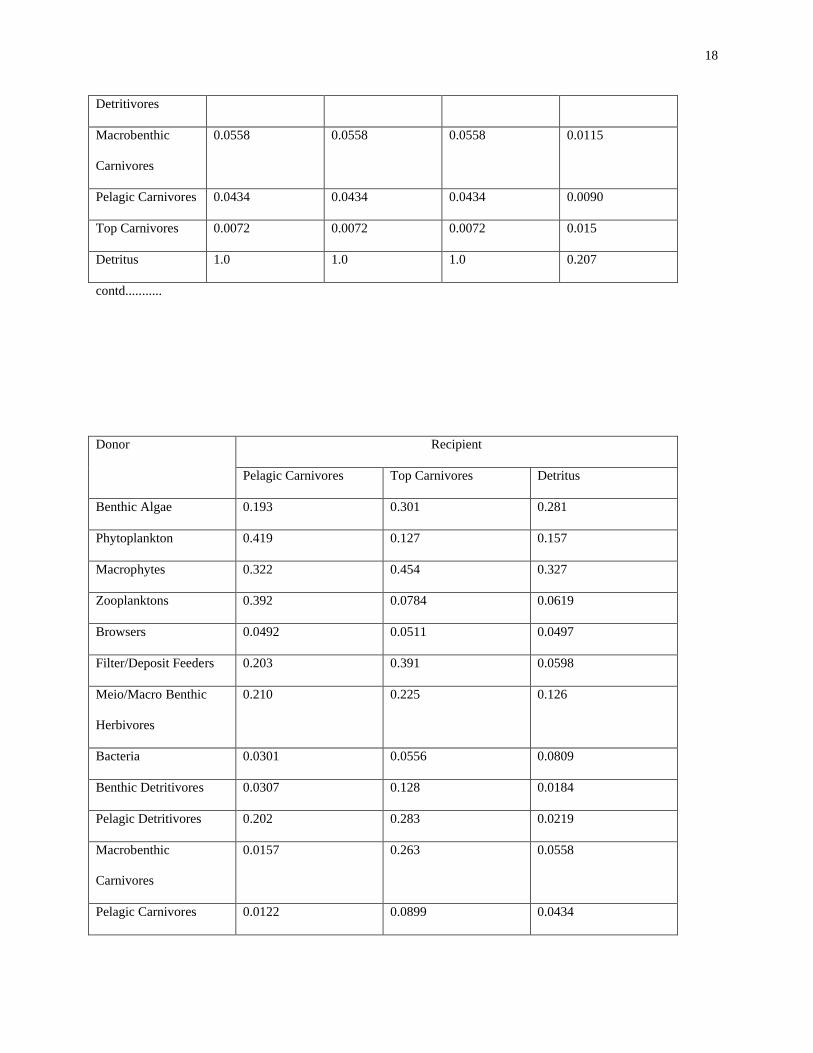
The total dependency matrix (Table 2), as defined above, conveys the fractions of the total input to a compartment

that flow from the various other taxa. Because energy may pass through several intermediate compartments in

getting from a given particular taxon to another, the columns of dependency coefficients usually add up to more than

1.0. In fact, the amount by which the column sum exceeds 1.0 is related to the average trophic position of that taxon

[28]. One is struck by the relative scarcity of any large dependencies (i.e., those near 1.0). The result helps to

strengthen the anecdotal observation that the system seems to possess a large redundancy of trophic pathways

(parallel routes), and therefore is probably highly resilient to subsequent perturbations, as one might expect from a

heavily impacted system.

We have studied the trophic level of each compartment by considering the total number of pathways feeding into

that compartment. As described above, the “Lindeman transformation matrix” partitions the energy flowing into

8

each consumer into discrete trophic fractions. The elements of the column of the Lindeman matrix can be weighted

by its corresponding trophic level to yield an effective trophic level for each consumer compartment (Fig. 2). This

exercise reveals that, although a slight degree of omnivory is exhibited by compartments 9-13, alternatively one may

aggregate all flows of each integer trophic length into a food chain that represents the underlying trophic status of

the starting food web (Fig. 3).

Alternatively, one may aggregate all flows of each integer trophic length into a food chain that represents the

underlying trophic status of the starting food web (Fig.3). That is, the Lindeman transformation matrix maps a

trophic web, as encountered in nature, into an abstract, but equivalent trophic “chain” of concatenated transfers. One

of the most interesting results concerns the ratio of herbivory:detritivory. Herbivory, the 2nd step in the grazing

chain, is 13400 kcal m-2 y-1, and detritivory is reported as 15700 units. That is they are virtually of the same

magnitude. Benthic dominated systems are usually characterized by a ratio of about 1:5 or less. In Chesapeake Bay

it is almost 1:10. In virgin mangrove system detritus is a major component, so that mangrove ecosystems are

generally referred to as detritus-based ecosystems. Here however the production of detritus and its input from

external source are very low, due to deforestation. Therefore, this system contains fewer detritivores. The pelagic

detritivores that remain consist mainly of the mullet group of fishes, and were recorded in this system only during

new moon and full moon, when tidal heights are greatest. In this mud flat, the benthic algae sustain a high rate of

herbivory, but their contributions to compartments 5,6 and 7 seem unexceptional. Herbivory appears to consist

largely of zooplankton grazing on phytoplankton and meiobenthos on macrophytes. The prominence of these

processes is highly unexpected in any type of mud flat. Three distinctly different zones are noted in this system:

ditches, flat areas, and some comparatively elevated areas. Zooplankton are confined mainly to the ditches,

macrophytes (particularly grasses and scanty Phoenix sp.) occupy the flat areas, and benthic algae are confined to

elevated areas. Bowsers (compartment 5), deposit/filter feeders and particularly macrobenthos are restricted mainly

to the grass beds. Only meiobenthos and a few macrobenthic fauna are found in the algal bed. This distribution

probably contributes to the dominance of these two modes of secondary production.

Counting primary producers and detritus as trophic level 1 results in an effective “trophic pyramid, as shown in

Fig.4.

9

Feedback via recycling is critical in determining overall system structure. Cycles in ecosystems constitute an

important factor that contributes to their autonomous behavior [29,30]. Cycle analysis reveals that only a small

number of cycles (31) exists in the Sundarban ecosystem. In addition, the Finn cycling index, which represents the

fraction to total activity that is devoted to recycling [11,31], indicates that only 8.4% of the total energy flow travels

over cyclical pathways. The low Finn cycling index and the small number of cycles in the system reinforce the

picture of the Sundarban as a highly disturbed ecosystem.

The total system throughput (T) measures the size of the system in terms of the aggregate activity of flow through

all its components. The value of T in this system is 136,570 kcal m-2 y-1 Because the mangrove biome is usually

considered to be a detritus based system, it is of utmost importance to calculate the fraction of total system

throughput that is subsidized by the mangrove litterfall. That fraction is very small: only 16% of the total system

input is comprised of litterfall. This proportion is very small in comparison to other mangrove systems, where the

corresponding values usually exceeds 95%. The main reason behind the small subsidy is the near total destruction of

major mangrove plants by human impacts.

Finally network analysis provides several information indices that characterize overall system status (Table 3). One

of the most revealing of these indices is the relative ascendancy, which gauges how much of the trophic complexity

appears in organized or constrained form. This index commonly runs from 35-45% in most ecosystems. The relative

ascendancy, in the Sundarban mangrove ecosystem is significantly lower (29%), however, and the relative

redundancy (unorganized complexity) is high (34%). These proportions reveal the extent of human impact upon this

ecosystem, which is fast disappearing. In most other applications to network data, these indices have exhibited very

little change in response to impacts. However, in this system the effects are quite dramatic and unmistakable. It is

hoped that these unequivocal results will alert other investigators to the utility of network analysis.

Last of all, we acknowledge that what we report here is but the beginning of the network analysis of the Sundarban

mangrove ecosystem. We certainly do not claim to have presented a complete picture of this ecosystem, especially

10

of the benthic system. In order to achieve a more complete treatment of the matter, we now turn our attention to the

undisturbed, virgin system of Sundarban mangroves.

4. Acknowledgements

The authors are greatly indebted to the Department of Mathematics, Jadavpur University for the use of computer

facilities. One of the authors (SR) is very thankful to the Susama Devichoudhurani Marine Biological Research

Institute, Sagar Island, Sundarban for field and laboratory facilities and the partial support from the granting agency

of the Ministry of Education, Youth and Sports of the Czech Republic (Project No. VS 96086 and 3070004) is

acknowledged. We are also thankful to Mr. Sandip Banerjee for assistance in preparing the manuscript. REU was

supported in part by the Across Trophic Levels Systems Simulation program of the United States Geological

Survey. (Contract 1445 - CA09 - 95 - 0093 SA#2).

References

[1] Asmus M L and McKellar Jr H N, Network analysis of the north inlet saltmarsh ecosystem. In Network Analysis

in Marine Ecology, Methods and Applications, ed. by Wulff F, Field J G and Mann K H (Springer-Verlag, NY,

1989) pp. 206-219.

[2] Baird, D. and R.E. Ulanowicz. The seasonal dynamics of the Chesapeake Bay ecosystem. Ecol. Monogr. 59

(1989) 329-364.

[3] Banerjee A K, Forests of Sundarban, Centenary commemoration volume,West Bengal Forests (DFO, Planning

and Statistical Cell, Writer,s Building, Calcutta, India, 1964).

[4] Bhunia A, Ecology of the tidal creeks and mudflats of Sagar Island (Sundarban) West Bengal. Ph.D. thesis,

Calcutta university, 1979.

[5] Boltzmann L, Weitere studien uber das Waermegleichtgewicht unter Gasmolekuelen. Wien. Ber. 66 (1872)

275-270.

[6] Choudhury A, Productivity of Sundarban mangrove ecosystem in both reclaimed and virgin island (DST, Govt.

of India, 1984).

[7] Choudhury A, Productivity of Sundarban mangrove ecosystem in both reclaimed and virgin island (DST, Govt.

of India, 1987).

11

[8] Ducklow H W, Fasham M J and Vezina A F, Derivation and analysis of flow networks for open ocean plankton

systems. In Network Analysis in Marine Ecology, Methods and Applications, ed. by Wulff F, Field J and Mann K H

(Springer-Verlag, NY, 1989) pp. 159-205.

[9] Ellison A M and Fransworth E J, Anthropogenic disturbance of Caribbean mangrove ecosystem: past impacts,

present trends and future predictions. Biotropica 28 (1996) 549-565.

[10] Field J G, Moloney C L and Attwood C G, Network analysis of simulated succession after an upwelling event.

In. Network Analysis in Marine Ecology, Methods and Applications, ed. by Wulff. F, Field J and Mann K H

(Springer-Verlag, NY, 1989) pp. 132-158.

[11] Finn J T, Measures of ecosystem structure and function derived from analysis of flows. J.Theor. Biol. 56 (1976)

363-380.

[12] Hannon J T, The structure of ecosystems. J. Theor. Biol. 41(1973) 535-546.

[13] Kay J J, Graham L A and Ulanowicz R E, A detailed guide to network analysis. In Network Analysis in Marine

Ecology, Methods and Applications, ed. by Wulff F, Field J and Mann K H. (Springer-Verlag, NY, 1989) pp. 15-61.

[14] Lawton J H, Feeding and food energy assimilation in larvae of the damselfly Pyrrhosoma nymphula (Sulz.)

(Odonata:Zygoptera) J. Anim. Ecol. 39 (1970) 669-689.

[15] Mitra D K, Mukherjee D, Roy A. B and Ray S, Permanent coexistence in a resource based competition system.

Ecol. Model 60 (1992) 77-85.

[16] Moore S T, Schuster M F and Harris F A, Radioisotope technique for estimating lady beetle consumption of

tobacco budworm eggs and larvae. J. Econ. Ent. 67 (1974) 703-705.

[17] Mukherjee D, Mitra D, Ray S and Roy A B, Effect of diffusion of two predators exploiting a resource.

Biosystems 31 (1993) 49-58.

[18] Mukherjee D, Ray S and Roy A B, Effect of timelag on a non living resource in a simple food chain.

Biosystems 39 (1996) 153-157.

[19] Nandi S, Ecology of benthic gastropods in the littoral mudflats and Hooghly estuary, India. Ph.D. thesis,

Calcutta University, 1986.

[20] Patten B C, Bosserman R W, Finn J T and Cale W J, Propagation of cause in ecosystems. In System Analysis

and Simulation in Ecology. vol. 4, ed. by Patten B C, (Academic Press, NY, 1976) pp. 457-579.

12

[21]Ramanathan A L and Subramanian V, Environmental geochemistry of the Pichavaram mangrove ecosystem

(tropical), southwest coast of India. Environmental geochemistry 37 (1999) 223-233.

[22] Ray S, Ecology of littoral larval dipterans (Arthropoda:Insecta) of the mangrove ecosystem of Sundarbans,

India. Ph.D. thesis, Calcutta University, l987.

[23] Sarkar A K, Mitra D, Ray S and Roy A B, Permanence and oscillatory co-existence of a detritus based

prey-predator model. Ecol. Model.53 (1991) 147-156.

[24] Southwood T R E, Ecological Methods with Particular reference to the Study of Insect Populations (Chapman

and Hall, NY, 1978).

[25] Steinke T D and Ward C J, Litter production by mangroves. II. St. Lucia (Estuary) and Richards Bay (South

Africa).S.Afr. J. Bot. 54 (1988) 445-454.

[26] Strickland J D H, Measuring the Production of Marine Phytoplanktons (Bull. Fish. Res. Bd. Canada, 1960).

[27] Strickland J D H and Parsons T R, A Practical handbook of Seawater Analysis. (Bull. Fish. Res. Bd. Canada,

1968).

[28] Szyrmer J and Ulanowicz R E, Total flows in ecosystems. Ecol. Model. 35 (1987) 123-136.

[29] Ulanowicz R E, Identifying the structure of cycling in ecosystems. Math. Biosci. 65 (1983) 219-237.

[30] Ulanowicz R E, Growth and Development: Ecosystem Phenomenology (Springer-Verlag, NY, 1986).

[31] Ulanowicz R E and Kemp W M, Towards canonical trophic aggregations. Amer. Nat. 114 (1979) 871-883.

[32] Warwick R M S and Radford P J, Analysis of the flow network in an estuarine benthic community. In Network

Analysis in Marine Ecology. Methods and Applications, ed. by Wulff F, Field J G and Mann K H (Springer-Verlag,

NY, 1989) pp. 220-231.

[33] Wiegert R G and Owen D F, Trophic structure, available resources and population density in terrestrial vs.

aquatic ecosystems. J. Theor. Biol. 30 (1971) 69-81.

[32] Wohlschlag D E, Difference in metabolic rates of migratory and resident freshwater forms of an arctic

whitefish. Ecology 38 (1957) 502-510.

[35] Wulff F and Ulanowicz R E, A comparative anatomy of the Baltic Sea and Chesapeake Bay ecosystems. In

Network Analysis in Marine Ecology. Methods and Applications. ed. by Wulff F, Field J G

and Mann K H (Springer-Verlag, NY, 1989) pp. 232-256.

13

Table 1

Donor Recipient

Zooplankton Browsers Filter/Deposit

Feeders

Meio/Macro

Benthic

Herbivores

Benthic Algae 0 0.0709 0.124 0.0994

Phytoplankton 0.551 0 0.0180 0

Macrophytes 0 0.0680 0.138 0

Zooplankton 0 0 0.0129 0

Browsers 0 0 0.0311 0

Filter/deposit

Feeders.

0 0 0.0175 0

Meio/Macro

Benthic herbivores

0 0 0.0292 0

Bacteria 0 0 0.0144 0

Benthic

detritivores

0 0 0.0038 0

Pelagic detritivores 0 0 0.0058 0

Macrobenthic 0 0 0.0202 0

14

carnivores

Pelagic Carnivores 0 0 0.0227 0

Top Carnivores 0 0 0.0060 0

Detritus 0 0 0.0382 0

contd.........

Donor Recipient

Bacteria Benthic

Detritivores

Pelagic

Detritivores

Macrobenthic

Carnivores

Benthic Alage 0.153 0.131 0.102 0.0873

Phytoplankton 0.101 0.0868 0.00677 0.0387

Macrophytes 0.146 0.125 0.117 0.0486

Zooplanktons 0.0726 0.0622 0.0590 0.156

Browsers 0.175 0.150 0.190 0.0588

Filter/Deposit

Feeders

0.0984 0.115 0.0106 0.0102

Meio/Macro

Benthic

Herbivores

0.164 0.141 0.241 0.0930

Bacteria 0.0809 0.115 0.0106 0.0102

Benthic

Detritivores

0.0214 0.0184 0.0485 0.0121

Pelagic

Detritivores

0.0327 0.0280 0.0170 0.1020

Macrobenthic 0.114 0.0974 0.0115 0.0109

15

Carnivores

Pelagic Carnivores 0.128 0.110 0.0130 0.0122

Top Carnivores 0.0339 0.0291 0.0034 0.0032

Detritus 0.216 0.185 0.0219 0.0021

contd.................

Donor Recipient

Pelagic Carnivores Top Carnivores Detritus

Benthic Alagae 0.0355 0.0348 0.708

Phytoplankton 0.0916 0.0174 0.470

Macrophytes 0.0486 0.0430 0.675

Zooplankton 0.156 0.0195 0.336

Browsers 0.0588 0.0384 0.813

Filter/Deposit Feeders 0.113 0.137 0.456

Meio/Macro Benthic

Herbivores

0.0930 0.0626 0.762

Bacteria 0.0102 0.0118 0.375

Benthic Detritivores 0.0121 0.0317 0.0993

Pelagic Detritivores 0.102 0.0901 0.152

Macrobenthic

Carnivores

0.0109 0.114 0.527

Pelagic Carnivores 0.0122 0.0564 0.594

Top Carnivores 0.0032 0.0037 0.157

Detritus 0.021 0.023 0.127

16

Table 2

Donor Recipient

Zooplankton Browsers Filter/Deposit

Feeders

Meio/Macro

Benthic

Herbivores

Benthic Alagae 0 0.461 0.376 0.239

Phytoplankton 1.00 0 0.0459 0

Macrophytes 0 0.539 0.509 0.761

Zooplanktons 0 0 0.0181 0

Browsers 0 0 0.0145 0

Filter/Deposit

Feeders

0 0 0.0175 0

Meio/Macro

Benthic

Herbivores

0 0 0.0367 0

Bacteria 0 0 0.0236 0

Benthic

Detritivores

0 0 0.0054 0

17

Pelagic

Detritivores

0 0 0.0064 0

Macrobenthic

Carnivores

0 0 0.0163 0

Pelagic Carnivores 0 0 0.0127 0

Top Carnivores 0 0 0.0021 0

Detritus 0 0 0.292 0

Contd.........................

Donor Recipient

Bacteria Benthic

Detritivores

Pelagic

Detritivores

Macrobenthic

Carnivores

Benthic Algae 0.281 0.281 0.281 0.293

Phytoplankton 0.157 0.157 0.157 0.122

Macrophytes 0.327 0.327 0.327 0.536

Zooplanktons 0.0619 0.0619 0.0619 0.103

Browsers 0.0497 0.0497 0.0497 0.110

Filter/Deposit

Feeders

0.0598 0.0598 0.0598 0.366

Meio/Macro

Benthic

Herbivores

0.126 0.126 0.126 0.375

Bacteria 0.0809 0.135 0.110 0.0217

Benthic

Detritivores

0.0184 0.0184 0.0184 0.0847

Pelagic 0.0219 0.0219 0.0219 0.0231

18

Detritivores

Macrobenthic

Carnivores

0.0558 0.0558 0.0558 0.0115

Pelagic Carnivores 0.0434 0.0434 0.0434 0.0090

Top Carnivores 0.0072 0.0072 0.0072 0.015

Detritus 1.0 1.0 1.0 0.207

contd...........

Donor Recipient

Pelagic Carnivores Top Carnivores Detritus

Benthic Algae 0.193 0.301 0.281

Phytoplankton 0.419 0.127 0.157

Macrophytes 0.322 0.454 0.327

Zooplanktons 0.392 0.0784 0.0619

Browsers 0.0492 0.0511 0.0497

Filter/Deposit Feeders 0.203 0.391 0.0598

Meio/Macro Benthic

Herbivores

0.210 0.225 0.126

Bacteria 0.0301 0.0556 0.0809

Benthic Detritivores 0.0307 0.128 0.0184

Pelagic Detritivores 0.202 0.283 0.0219

Macrobenthic

Carnivores

0.0157 0.263 0.0558

Pelagic Carnivores 0.0122 0.0899 0.0434

19

Top Carnivores 0.0020 0.0037 0.0072

Detritus 0.282 0.506 0.127

Table 3

Total System Throughput 136570

Development Capacity 700300

Ascendency 204250

Overhead of Imports 89349

Overhead of Exports 37615

Dissipative Overhead 134300

Redundency 234790

Finn Cycling Index 0.08375

20

Legends for figures:

Fig. 1. The diagram of energy flows among 14 compartments of the network of the benthic food web of the

Sundarban mangrove ecosystem. All flows are in (kcal m-2 y-1) and standing stock densities in (kcal m-2). The

ground symbols represent respiratory losses. The arrows connecting one compartment to other represent flows and

the arrows from outside to compartment and also from compartments to outside represent inflow and outflow

respectively.

Fig. 2 The effective trophic positions of each taxon in 17 compartments food web model of Sundarban mangrove

ecosystem.

Fig. 3 The trophic aggregation of the Sundarban mangrove benthic network with the autotrophs and detritus

separated and mapped into Lindeman-type trophic levels. The trophic levels are designated by Roman numerals (= I

– V, and D – represents the detritus pool).

Fig. 4 The trophic aggregation shown in Fig. 3, except the primary producers and the detritus have been merged (I +

D), yielding a true “trophic pyramid”.

Legends for tables:

21

Table 1 Total contribution coeffcient which represents the fractions a component contributed to the “diets” of other

components.

Table 2 Total dependency coefficient which represents the fraction of the total amount of energy leaving one

compartment eventually enters another compartment, via both direct food chains and cycling.

Table 3 Showing the information indices (kcal m-2 y-1)