net power output and pressure drop behavior of pem …
TRANSCRIPT

NET POWER OUTPUT AND PRESSURE DROP BEHAVIOR OF
PEM FUEL CELLS WITH SERPENTINE AND INTERDIGITATED
FLOW FILEDS
by
Fang Ruan
A thesis submitted to the Faculty of the University of Delaware in partial
fulfillment of the requirements for the degree of Master of Science in Mechanical
Engineering
Spring 2014
© 2014 Fang Ruan
All Rights Reserved

All rights reserved
INFORMATION TO ALL USERSThe quality of this reproduction is dependent upon the quality of the copy submitted.
In the unlikely event that the author did not send a complete manuscriptand there are missing pages, these will be noted. Also, if material had to be removed,
a note will indicate the deletion.
Microform Edition © ProQuest LLC.All rights reserved. This work is protected against
unauthorized copying under Title 17, United States Code
ProQuest LLC.789 East Eisenhower Parkway
P.O. Box 1346Ann Arbor, MI 48106 - 1346
UMI 1562417
Published by ProQuest LLC (2014). Copyright in the Dissertation held by the Author.
UMI Number: 1562417
NET POWER OUTPUT AND PRESSURE DROP BEHAVIOR OF
PEM FUEL CELLS WITH SERPENTINE AND INTERDIGITATED
FLOW FIELDS
by
Fang Ruan
Approved: __________________________________________________________
Ajay Prasad, Ph.D.
Professor in charge of thesis on behalf of the Advisory Committee
Approved: __________________________________________________________
Suresh Advani, Ph.D.
Professor in charge of thesis on behalf of the Advisory Committee
Approved: __________________________________________________________
Suresh Advani, Ph.D.
Chair of the Department of Mechanical Engineering
Approved: __________________________________________________________
Babatunde Ogunnaike, Ph.D.
Dean of the College of Engineering

Approved: __________________________________________________________
James G. Richards, Ph.D.
Vice Provost for Graduate and Professional Education

iv
ACKNOWLEDGMENTS
I would like to thank the Fuel Cell Research Lab and the Federal Transit
Administration for funding me throughout my graduate studies. This program
provided me precious and unique opportunity to get involved in cutting-edge research
in sustainable energy, and it also inspired my interest in working in the renewable
energy industry in my future career.
First and foremost, I would also like express my deepest gratitude to both of
my advisors: Dr. Ajay Prasad and Dr. Suresh Advani. Their vast knowledge, great
vision combined with the consistent guidance in technical details providing me
tremendous help throughout my research work in the past two years. They also offered
me the freedom to explore my own research interest as well as encouragement and
guidance when I meet difficulties and frustration. Without their excellent advisement, I
would not be able to finish this thesis and reach my academic goals.
My sincere gratitude is also given to all of the Fuel Cell Research Lab
associates for their help with various stages of my project. In particular, I owe thanks
to Dr. Liang Wang for offering lab training, general knowledge and deep
understanding in PEM fuel cell principles and testing, tenacity to help to solve
problems that I encountered, Andrew Baker for his help with generating SolidWorks
drawings for manufacturing, Yongqiang Wang for his help with setting up pressure
measurement equipment, Jaehyung Park for his advice and help with fuel cell test
training, and Adam Kinzey for his help with manufacturing parts for the Arbin fuel

v
cell test stand. I also want to thank Mr. Steve Beard for his guidance and help in
machining the metal parts for the PEM fuel cell in the Spencer machine shop.
I especially thank my parents, for their continued support, love, concern and
motivation throughout all of my endeavors. I also would like to thank my boyfriend
Chenglong Zheng for his consistent love, support and understanding in the past two
years. I’m also thankful to all my friends for the enjoyable time we shared and great
help they provided in work and in life.
Most importantly, I want to give my thanks to my dear God, who has led and
sustained me through my life, and always been with me in my best and toughest times.
Grace from God is the major source of my strength, ability and enjoyment.
vi
TABLE OF CONTENTS
LIST OF FIGURES ................................................................................................. ix
LIST OF TABLES ................................................................................................. xvi
ABSTRACT .......................................................................................................... xvi
Chapter
1 INTRODUCTION .............................................................................................. 1
1.1 Overview of PEM Fuel Cells .................................................................... 1
1.2 Previous Studies on Fuel Cell Power Analysis and Pressure Drop
Behavior .................................................................................................... 5
1.3 Research Objectives and Test Procedures ................................................. 8
1.4 Thesis Overview ...................................................................................... 11
2 EXPERIMENT SETUP AND TEST PROCEDURE ....................................... 12
2.1 Fuel Cell Components and Design .......................................................... 12
2.2 Fuel Cell Test Station .............................................................................. 13
2.3 Pressure Measurement Station ................................................................ 14
2.4 Test Procedure ......................................................................................... 16
2.5 Summary .................................................................................................. 16
3 RESULTS OF NET POWER WITH DIFFERENT FLOW FIELD
COMBINATIONS ............................................................................................ 17
3.1 Pressure Drop in Four Flow Fields Combinations .................................. 17
3.2 Effect of Operating Conditions on Pressure Drop ................................... 22
3.3 Parasitic Power Loss Calculation and Net Power ................................... 26
3.4 Power Efficiency Discussion ................................................................... 30
3.5 Effect of Operating Conditions on Net Power Output and Power
Efficiency ................................................................................................ 30
3.6 Summary .................................................................................................. 48
4 PRESSURE DROP BEHAVIOR IN PEM FUEL CELLS UNDER
FLUCTUATING HUMIDIFICATION TEMPERATURES ............................. 50
4.1 Correlation Between Fuel Cell Voltage and Anode Pressure Drop ......... 50
4.2 Correlation Between Fuel Cell Current Density and Pressure Drop ....... 56

vii
4.3 Correlation Coefficients .......................................................................... 59
4.4 Discussion ................................................................................................ 60
4.5 Summary .................................................................................................. 61
5 CONCLUSION AND FUTURE WORK ......................................................... 62
REFERENCES ....................................................................................................... 65
Appendix
A CALCULATION OF COMPRESSOR POWER…. .......................................... 68
B PRESSURE DROP AND CELL OUTPUT DATA… ......................................... 73
C PERMISSION FOR FIGURE USAGE… .......................................................... 92
viii
LIST OF FIGURES
Figure 1.1 Structure of PEM fuel cell and associated chemical reactions [3] ............ 3
Figure 1.2 Schematics of single serpentine, parallel and interdigitated flow field
design [4] ................................................................................................... 4
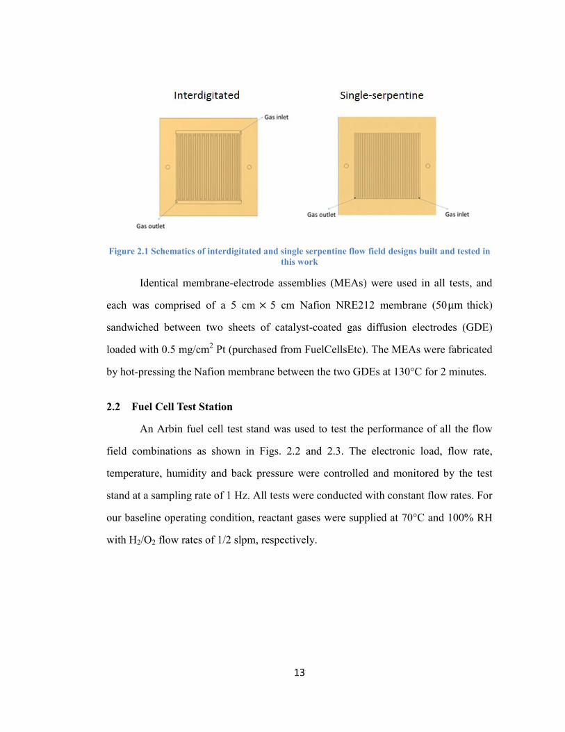
Figure 2.1 Schematics of interdigitated and single serpentine flow field designs built
and tested in this work ............................................................................. 13
Figure 2.2 Details of the Arbin fuel cell test stand ................................................... 14
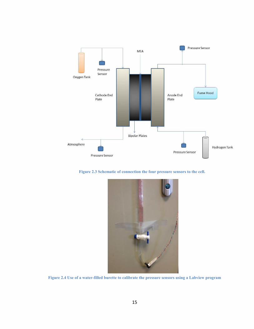
Figure 2.3 Schematic of connection the four pressure sensors to the cell. ............... 15
Figure 2.4 Use of a water-filled burette to calibrate the pressure sensors using a
Labview program ..................................................................................... 15
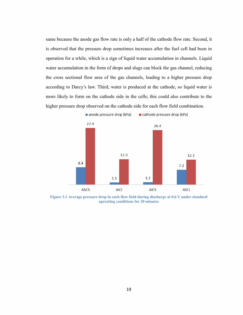
Figure 3.1 Average pressure drop in each flow field during discharge at 0.6 V
under standard operating conditions for 30 minutes ............................... 19
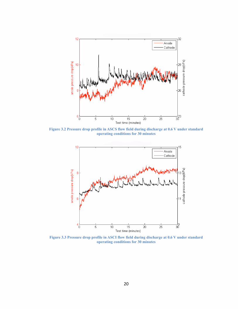
Figure 3.2 Pressure drop profile in ASCS flow field during discharge at 0.6 V
under standard operating conditions for 30 minutes ............................... 20
Figure 3.3 Pressure drop profile in ASCI flow field during discharge at 0.6 V
under standard operating conditions for 30 minutes ............................... 20
Figure 3.4 Pressure drop profile in AICS flow field during discharge at 0.6 V
under standard operating conditions for 30 minutes ............................... 21
Figure 3.5 Pressure drop profile in AICI flow field during discharge at 0.6 V under
standard operating conditions for 30 minutes ......................................... 21
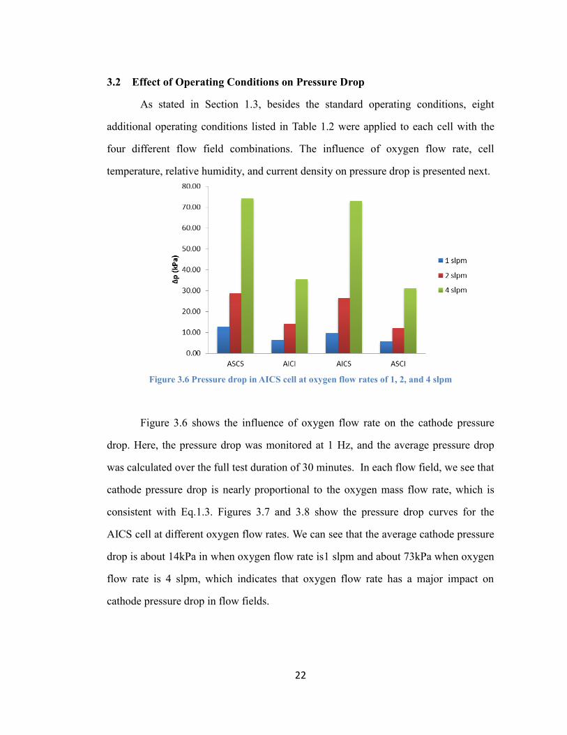
Figure 3.6 Pressure drop in AICS cell at oxygen flow rates of 1, 2, and 4 slpm ...... 22
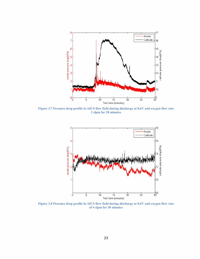
Figure 3.7 Pressure drop profile in AICS flow field during discharge at 0.6V and
oxygen flow rate 1 slpm for 30 minutes .................................................. 23
Figure 3.8 Pressure drop profile in AICS flow field during discharge at 0.6V and
oxygen flow rate of 4 slpm for 30 minutes .............................................. 23

ix
Figure 3.9 Average pressure drop in each flow field during discharge at 0.6 V for
30 minutes at 60°C and 70°C .................................................................. 24
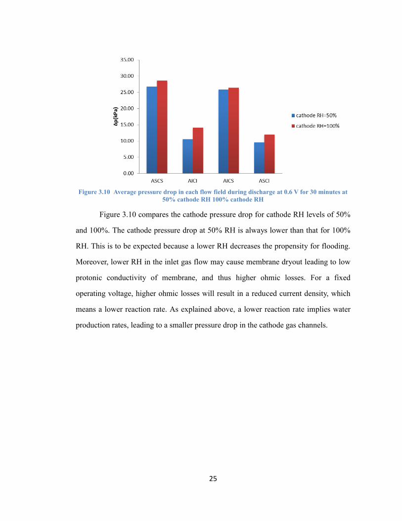
Figure 3.10 Average pressure drop in each flow field during discharge at 0.6 V for
30 minutes at 50% cathode RH 100% cathode RH ................................. 25
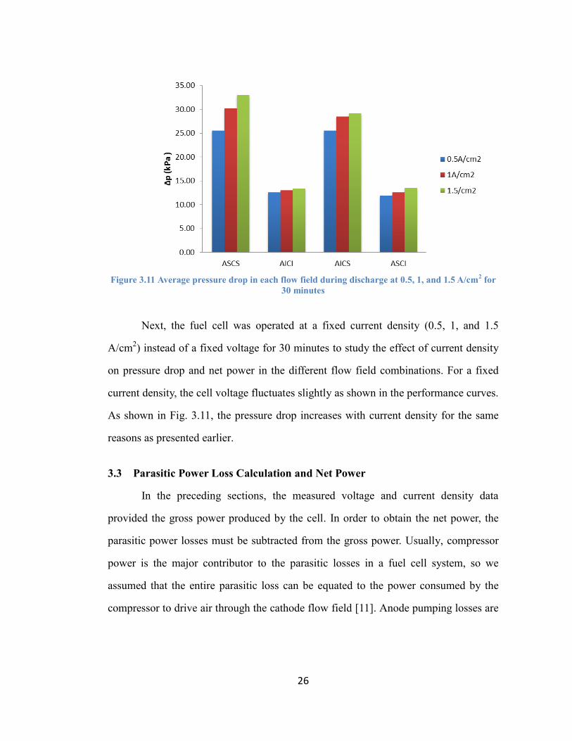
Figure 3.11 Average pressure drop in each flow field during discharge at 0.5, 1,
and 1.5 A/cm2 for 30 minutes .................................................................. 26
Figure 3.12 Average total power output, parasitic power loss and net power in each
cell; cells were operated at standard operating conditions for 30
minutes at 0.6 V. Net power is defined as the difference between total
power output and parasitic power loss. The quoted values are in watts. . 28
Figure 3.13 Average net power in each cell; cells were operated at standard
operating condition for 30 minutes at 0.6 V. Standard deviations were
calculated from three tests for total power output and parasitic loss to
assess variations in test results within the same group of experiments. .. 28
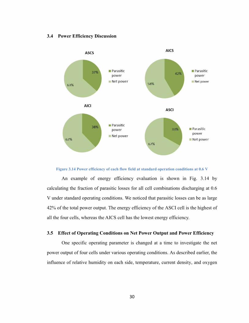
Figure 3.14 Power efficiency of each flow field at standard operation conditions at
0.6 V ........................................................................................................ 30
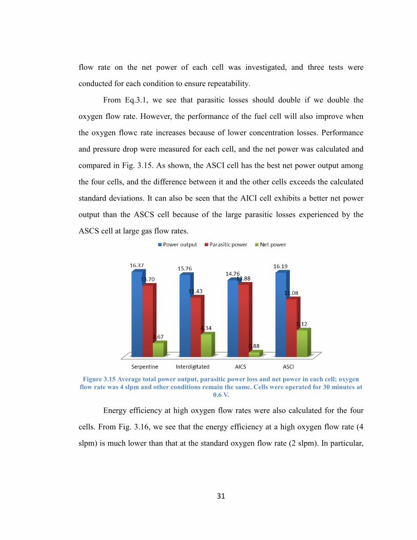
Figure 3.15 Average total power output, parasitic power loss and net power in each
cell; oxygen flow rate was 4 slpm and other conditions remain the
same. Cells were operated for 30 minutes at 0.6 V. ................................. 31
Figure 3.16 Power efficiency of each flow field at oxygen flow rate of 4 slpm at
0.6 V ........................................................................................................ 32
Figure 3.17 Current density and voltage profile of ASCI cell during discharge at
0.6V and oxygen flow rate of 4 slpm for 30 minutes .............................. 33
Figure 3.18 Average total power output, parasitic power loss and net power in each
cell; oxygen flow rate was 1 slpm and other conditions remain the
same. Cells were operated for 30 minutes at 0.6 V. ................................. 34
Figure 3.19 Power efficiency of each flow field at oxygen flow rate of 1 slpm at
0.6 V ........................................................................................................ 35
Figure 3.20 Current density and voltage profile of ASCI cell during discharge at
0.6V and oxygen flow rate of 1 slpm for 30 minutes .............................. 35
x
Figure 3.21 Average total power output, parasitic power loss and net power in each
cell; cell temperature was 60°C and other conditions remain the same.
Cells were operated for 30 minutes at 0.6 V. ........................................... 37
Figure 3.22 Power efficiency of each flow field at cell temperature of 60°C and
0.6 V ........................................................................................................ 38
Figure 3.23 Current density and voltage profile of ASCI cell during discharge at
0.6V and 60°C for 30 minutes ................................................................. 38
Figure 3.24 Average total power output, parasitic power loss and net power in each
cell; anode RH was 50% and other conditions remain the same. Cells
were operated for 30 minutes at 0.6 V..................................................... 39
Figure 3.25 Average total power output, parasitic power loss and net power in each
cell; cathode RH was 50% and other conditions remain the same. Cells
were operated for 30 minutes at 0.6 V. .................................................... 40
Figure 3.26 Power efficiency of each flow field at anode RH 50% and 0.6 V .......... 40
Figure 3.27 Power efficiency of each flow field at cathode RH 50% and 0.6 V ....... 41
Figure 3.28 Current density and voltage profile of ASCI cell during discharge at
0.6V and anode RH 50% for 30 minutes ................................................. 41
Figure 3.29 Current density and voltage profile of ASCI cell during discharge at
0.6V at cathode RH 50% for 30 minutes ................................................. 42
Figure 3.30 Average total power output, parasitic power loss and net power in each
cell; cells were operated at standard operating conditions for 30
minutes at 0.5 A/cm2 ................................................................................ 43
Figure. 3.31 Average total power output, parasitic power loss and net power in each
cell; cells were operated at standard operation condition for 30 minutes
discharging at 1A/cm2. ............................................................................ 44
Figure 3.32 Average total power output, parasitic power loss and net power in each
cell; cells were operated at standard operating conditions for 30
minutes at 1.5 A/cm2 ................................................................................ 44
Figure 3.33 Power efficiency of each flow field at standard operating conditions
and 0.5 A/cm2 .......................................................................................... 44
Figure 3.34 Power efficiency of each flow field at standard operating conditions
and 1 A/cm2 ........................................................................................... 45

xi
Figure 3.35 Power efficiency of each flow field at standard operating conditions
and 1.5 A/cm2 .......................................................................................... 46
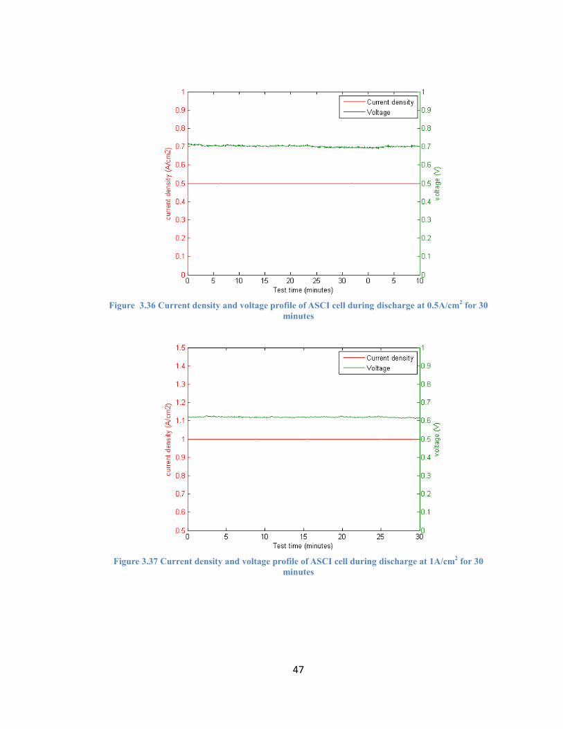
Figure 3.36 Current density and voltage profile of ASCI cell during discharge at
0.5A/cm2 for 30 minutes .......................................................................... 47
Figure 3.37 Current density and voltage profile of ASCI cell during discharge at
1A/cm2 for 30 minutes ............................................................................. 47
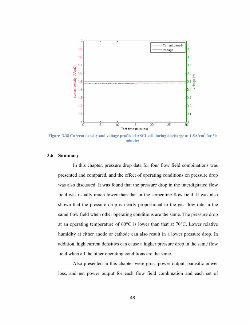
Figure 3.38 Current density and voltage profile of ASCI cell during discharge at
1.5A/cm2 for 30 minutes .......................................................................... 48
Figure 4.1 Pressure drop profile in each flow field at 0.5 A/cm2 after switching
from OCV (2 slpm oxygen flow rate); anode humidification
temperature fluctuates in the range of ± 20°C. Upper left: ASCS;
Upper right: AICI; Lower left: AICS; Lower right: ASCI. ..................... 51
Figure 4.2 AICI cell test at 0.5 A/cm2. Upper left: fuel cell performance data;
lower left: anode and cathode pressure drop; right: anode pressure drop
and voltage data ....................................................................................... 52
Figure 4.3 AICI cell test at 0.5 A/cm2. Upper: time evolution over 30 min of
current density overlaid with the anode pressure drop. The other two
sub-plots are close-up views of the two spikes over a narrow time
span. ......................................................................................................... 53
Figure 4.4 Humidification temperature and voltage data for the AICI cell at 0.5
A/cm2 for 30 minutes ............................................................................... 55
Figure 4.5 ASCI cell test at 0.6 V. Upper left: fuel cell performance data; lower
left: anode and cathode pressure drop; right: anode pressure drop and
voltage data .............................................................................................. 56
Figure 4.6 ASCI cell test at 0.6 V. Upper left: time evolution over 30 min of current
density overlaid with the anode pressure drop. The other three sub-plots
are close-up views of the three spikes over a narrow time span. ............ 58
Figure 4.7 Humidification temperature and voltage data for the ASCI cell at 0.6 V
for 30 minutes .......................................................................................... 59
Figure 4.8 Correlation coefficients of anode pressure drop and cell current density
at 0.6 V .................................................................................................... 60

xii
Figure 4.9 Correlation coefficients of anode pressure drop and cell voltage at
0.5A/cm2 .................................................................................................. 60
Figure B.1 Pressure drop profile in ASCI flow field during discharge at 0.6V and
oxygen flow rate of 1 slpm for 30 minutes .............................................. 73
Figure B.2 Pressure drop profile in AICI flow field during discharge at 0.6V and
oxygen flow rate of 1 slpm for 30 minutes .............................................. 74
Figure B.3 Pressure drop profile in ASCS flow field during discharge at 0.6V and
oxygen flow rate of 1 slpm for 30 minutes .............................................. 75
Figure B.4 Pressure drop profile in ASCI flow field during discharge at 0.6V and
oxygen flow rate of 4 slpm for 30 minutes .............................................. 75
Figure B.5 Pressure drop profile in AICI flow field during discharge at 0.6V and
oxygen flow rate of 4 slpm for 30 minutes .............................................. 76
Figure B.6 Pressure drop profile in ASCS flow field during discharge at 0.6V and
oxygen flow rate of 4 slpm for 30 minutes .............................................. 76
Figure B.7 Pressure drop profile in ASCI flow field during discharge at 0.6V
cathode RH 50% for 30 minutes ............................................................. 77
Figure B.8 Pressure drop profile in AICI flow field during discharge at 0.6V and
cathode RH 50% for 30 minutes ............................................................. 77
Figure B.9 Pressure drop profile in ASCS flow field during discharge at 0.6V and
cathode RH 50% for 30 minutes ............................................................. 78
Figure B.10 Pressure drop profile in ASCI flow field during discharge at 0.6V and
60°C for 30 minutes................................................................................. 78
Figure B.11 Pressure drop profile in AICS flow field during discharge at 0.6V and
60°C for 30 minutes................................................................................. 79
Figure B.12 Pressure drop profile in AICI flow field during discharge at 0.6V and
60°C for 30 minute .................................................................................. 79
Figure B.13 Pressure drop profile in ASCI flow field during discharge at 0.6V and
60°C for 30 minutes................................................................................. 80
Figure B.14 Performance profile in AICI flow field during discharge at 0.6V under
standard operating condition for 30 minutes ........................................... 80
xiii
Figure B.15 Performance profile in ASCS flow field during discharge at 0.6V
under standard operating condition for 30 minutes ................................. 81
Figure B.16 Performance in ASCI flow field during discharge at 0.6V under
standard operating condition for 30 minutes ........................................... 81
Figure B.17 Performance profile in AICS flow field during discharge at 0.6V under
standard operating condition for 30 minutes ........................................... 82
Figure B.18 Performance profile in AICS flow field during discharge at 0.6V and
60°C for 30 minutes................................................................................. 82
Figure B.19 Performance profile in ASCS flow field during discharge at 0.6V and
60°C for 30 minutes................................................................................. 83
Figure B.20 Performance profile in AICI flow field during discharge at 0.6V and
60°C for 30 minutes................................................................................. 83
Figure B.21 Performance profile in AICS flow field during discharge at 0.6V and
cathode RH 50% for 30 minutes ............................................................. 84
Figure B.22 Performance profile in AICI flow field during discharge at 0.6V
cathode RH 50% for 30 minutes ............................................................. 84
Figure B.23 Performance profile in ASCS flow field during discharge at 0.6V and
cathode RH 50% for 30 minutes ............................................................. 85
Figure B.24 Performance profile in AICS flow field during discharge at 0.6V and
oxygen flow rate of 4 slpm for 30 minutes .............................................. 85
Figure B.25 Performance profile in AICI flow field during discharge at 0.6V and
oxygen flow rate of 4 slpm for 30 minutes .............................................. 86
Figure B.26 Performance profile in ASCS flow field during discharge at 0.6V and
oxygen flow rate of 4 slpm for 30 minutes .............................................. 86
Figure B.27 Performance profile in ASCS flow field during discharge at 0.5A/cm2
for 30 minutes .......................................................................................... 87
Figure B.28 Performance profile in AICS flow field during discharge at 0.5A/cm2
for 30 minutes .......................................................................................... 87
Figure B.29 Performance profile in AICI flow field during discharge at 0.5A/cm2
for 30 minutes .......................................................................................... 88

xiv
Figure B.30 Performance profile in AICS flow field during discharge at 1.0A/cm2
for 30 minutes .......................................................................................... 88
Figure B.31 Performance profile in AICI flow field during discharge at 1.0A/cm2
for 30 minutes .......................................................................................... 89
Figure B.32 Performance profile ASCS flow field during discharge at 1.0A/cm2 for
30 minutes ............................................................................................... 89
Figure B.33 Performance profile AICS flow field during discharge at 1.5A/cm2 for
30 minutes ............................................................................................... 90
Figure B.34 Performance profile in AICI flow field during discharge at 1.5A/cm2
for 30 minutes .......................................................................................... 90
Figure B.35 Performance profile in ASCS flow field during discharge at 1.5A/cm2
for 30 minutes .......................................................................................... 91
xv
LIST OF TABLES
Table 1.1 Flow field combinations used in this work ................................................ 9
Table 1.2 Operating conditions employed in tests (green area is the base line) ...... 10
Table 3.1 P-values for the net power results for the ASCI and ASCS flow fields at
each specific operating condition ............................................................ 29
Table A.1 Voltage=0.6V; oxygen flow rate=2 slpm; temperature=70°C; anode
RH=50%; cathode RH=100% ................................................................. 69
Table A.2 Voltage=0.6V; oxygen flow rate=2; slpm temperature=70°C; anode
RH=100%; cathode RH=50% ................................................................. 69
Table A.3 Voltage=0.6V; oxygen flow rate=1 slpm; temperature=70°C; anode
RH=100%; cathode RH=100% ............................................................... 70
Table A.4 Voltage=0.6V; oxygen flow rate=4; slpm temperature=70°C; anode
RH=100%; cathode RH=100% ............................................................... 70
Table A.5 Voltage=0.6V; oxygen flow rate=2; slpm temperature=60°C; anode
RH=100%; cathode RH=100% ............................................................... 71
Table A.6 Voltage=0.6V; oxygen flow rate=2; slpm temperature=70°C; anode
RH=100%; cathode RH=100% ............................................................... 71
Table A.7 Current density 1A/cm2 ;oxygen flow rate=2; slpm temperature=70°C;
anode RH=100%; cathode RH = 100% ................................................... 72
Table A.8 Current density=1.5A/cm2 ;oxygen flow rate=2; slpm temperature=
70°C; anode RH=100%; cathode RH=100% .......................................... 72
Table A.9 Current density=0.5A/cm2 ;oxygen flow rate=2; slpm temperature=
70°C; anode RH=100%; cathode RH=100% .......................................... 72
xvi
ABSTRACT
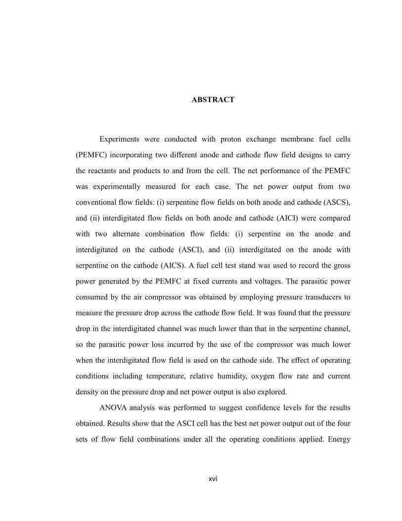
Experiments were conducted with proton exchange membrane fuel cells
(PEMFC) incorporating two different anode and cathode flow field designs to carry
the reactants and products to and from the cell. The net performance of the PEMFC
was experimentally measured for each case. The net power output from two
conventional flow fields: (i) serpentine flow fields on both anode and cathode (ASCS),
and (ii) interdigitated flow fields on both anode and cathode (AICI) were compared
with two alternate combination flow fields: (i) serpentine on the anode and
interdigitated on the cathode (ASCI), and (ii) interdigitated on the anode with
serpentine on the cathode (AICS). A fuel cell test stand was used to record the gross
power generated by the PEMFC at fixed currents and voltages. The parasitic power
consumed by the air compressor was obtained by employing pressure transducers to
measure the pressure drop across the cathode flow field. It was found that the pressure
drop in the interdigitated channel was much lower than that in the serpentine channel,
so the parasitic power loss incurred by the use of the compressor was much lower
when the interdigitated flow field is used on the cathode side. The effect of operating
conditions including temperature, relative humidity, oxygen flow rate and current
density on the pressure drop and net power output is also explored.
ANOVA analysis was performed to suggest confidence levels for the results
obtained. Results show that the ASCI cell has the best net power output out of the four
sets of flow field combinations under all the operating conditions applied. Energy

xvii
efficiency is calculated for each case, and the influence of the flow field combination
and operating conditions on energy efficiency is presented.
1
Chapter 1
INTRODUCTION
1.1 Overview of PEM Fuel Cells
Environmental concerns about modern society’s dependence upon reliable
energy sources and global warming have created the need for sustainable energy
sources with high energy-conversion efficiency. Among various technologies
developed to reduce the consumption of fossil fuels, hydrogen-powered fuel cells are a
promising alternative. Proton exchange membrane fuel cell (PEMFC), which is also
called solid polymer fuel cell (SPFC), is a device that can convert chemical energy
directly into electrical energy through an electrochemical reaction between hydrogen
and oxygen in the presence of a catalyst. The only byproduct of this electrochemical
process is water and heat, which makes it environment-friendly. The well-to-wheel
energy efficiency for fuel cells is higher than conventional energy conversion devices
such as the internal combustion engine for automotive applications, and the steam
turbine for stationary power applications [1]. The low operating temperature of the
PEMFC guarantees a quick startup and safe operation for automotive applications.
There are no moving parts in the PEMFC, which increases its life span, and also
reduces operating noise [2]. Based on all the advantages mentioned above, the
PEMFC has been considered as one of the best renewable energy sources for the
automotive and portable electronics industries for its high power density, clean
operation, low operating temperature, and high energy efficiency.
2
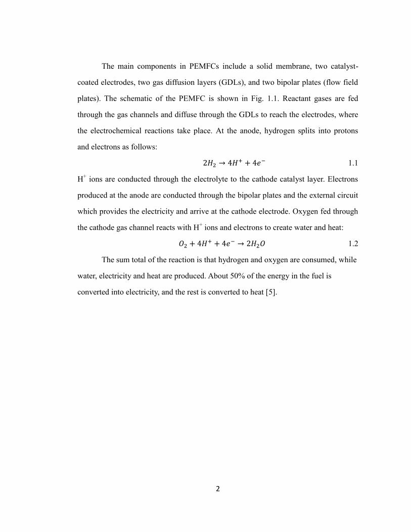
The main components in PEMFCs include a solid membrane, two catalyst-
coated electrodes, two gas diffusion layers (GDLs), and two bipolar plates (flow field
plates). The schematic of the PEMFC is shown in Fig. 1.1. Reactant gases are fed
through the gas channels and diffuse through the GDLs to reach the electrodes, where
the electrochemical reactions take place. At the anode, hydrogen splits into protons
and electrons as follows:
2𝐻2 → 4𝐻+ + 4𝑒− 1.1
H+ ions are conducted through the electrolyte to the cathode catalyst layer. Electrons
produced at the anode are conducted through the bipolar plates and the external circuit
which provides the electricity and arrive at the cathode electrode. Oxygen fed through
the cathode gas channel reacts with H+ ions and electrons to create water and heat:
𝑂2 + 4𝐻+ + 4𝑒− → 2𝐻2𝑂 1.2
The sum total of the reaction is that hydrogen and oxygen are consumed, while
water, electricity and heat are produced. About 50% of the energy in the fuel is
converted into electricity, and the rest is converted to heat [5].
3
Figure 1.1 Structure of PEM fuel cell and associated chemical reactions [3]
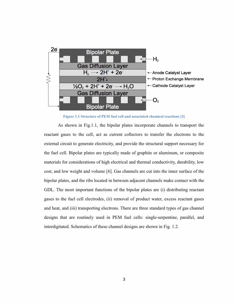
As shown in Fig.1.1, the bipolar plates incorporate channels to transport the
reactant gases to the cell, act as current collectors to transfer the electrons to the
external circuit to generate electricity, and provide the structural support necessary for
the fuel cell. Bipolar plates are typically made of graphite or aluminum, or composite
materials for considerations of high electrical and thermal conductivity, durability, low
cost, and low weight and volume [6]. Gas channels are cut into the inner surface of the
bipolar plates, and the ribs located in between adjacent channels make contact with the
GDL. The most important functions of the bipolar plates are (i) distributing reactant
gases to the fuel cell electrodes, (ii) removal of product water, excess reactant gases
and heat, and (iii) transporting electrons. There are three standard types of gas channel
designs that are routinely used in PEM fuel cells: single-serpentine, parallel, and
interdigitated. Schematics of these channel designs are shown in Fig. 1.2.

4
Figure 1.2 Schematics of single serpentine, parallel and interdigitated flow field design [4]
The material and geometry of the channels inscribed in the bipolar plate can
have a major influence on the PEM fuel cell’s overall performance due to the role it
plays in gas and electron transport, and water and heat management. Spernjak et al. [7]
compared the performance and power output of PEM fuel cells with parallel, single-
serpentine and interdigitated flow fields, and found that the single-serpentine flow
field yielded the best and most stable output; the interdigitated flow field exhibited
performance which was comparable to the single-serpentine cell except at high current
densities, whereas the parallel cell exhibited much lower and unstable output.
Besides the flow field’s influence on cell output, the performance of PEMFCs
is also influenced by the operating conditions such as the operating pressure,
temperature, relative humidity (RH), and flow rates of reactant gases. Parametric
studies of operating conditions has been carried out by Wang et al. [9], and the
experimental results showed the effects of operating temperature, anode/cathode RH,
operating pressure, and various combinations of these parameters. Higher pressure in
the cell can boost its performance according to the Nernst equation and reduce mass
transport voltage losses at high current densities. Balasubramanin et al. [10] also
revealed that higher operating pressures can improve fuel cell performance. The

5
voltage of a single fuel cell was improved from 0.5 V to 0.6 V at a current density of
1200 mA/cm2 when the operating pressure was increased from 170 kPa to 300 kPa.
However, the power consumed by the compressor also increased by 100% when the
pressure was increased from 170 kPa to 300 kPa, which increases the parasitic power
loss by 30%. This parasitic power loss has to be subtracted from the fuel cell’s total
power output, thus offsetting the voltage gain at higher operating pressures.
To supply reactant gases and operate the fuel cell under selected operating
conditions, auxiliary components are needed in the fuel cell system. Pumps, fans,
compressors, blowers, heaters, humidifiers, and a cooling system are the major
components in the gas supply and thermal management system. Among these
components, the air compressor is the major source of power loss in the fuel cell
system. Air must be compressed and driven into fuel cell system by the compressor,
and work is done on the gas to raise its pressure and temperature. In this work, we
define the parasitic power loss as the power consumed by the compressor, which is a
function of the pressure drop inside the fuel cell, as described in Chapter 2. A previous
study showed that the typical compressor power consumption would be about 20% or
more of the total power generated [10]. Flow field designs that cause a higher pressure
drop across the flow field channel will increase the reactant pumping power and
reduce the system performance [6, 11]. Spernjak et al. [7] also showed that water
dynamics and parasitic power loss (the power needed to pump the reactant gases
through the flow field) in different flow fields might vary substantially.
1.2 Previous Studies on Fuel Cell Power Analysis and Pressure Drop Behavior
Pressure requirements to pump the reactant gases at a given mass flow rate will
depend on the flow field design. For a given width and height of the flow channel, the
6
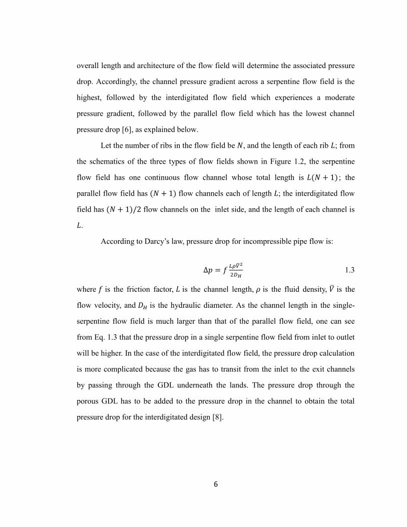
overall length and architecture of the flow field will determine the associated pressure
drop. Accordingly, the channel pressure gradient across a serpentine flow field is the
highest, followed by the interdigitated flow field which experiences a moderate
pressure gradient, followed by the parallel flow field which has the lowest channel
pressure drop [6], as explained below.
Let the number of ribs in the flow field be 𝑁, and the length of each rib 𝐿; from
the schematics of the three types of flow fields shown in Figure 1.2, the serpentine
flow field has one continuous flow channel whose total length is 𝐿(𝑁 + 1) ; the
parallel flow field has (𝑁 + 1) flow channels each of length 𝐿; the interdigitated flow
field has (𝑁 + 1)/2 flow channels on the inlet side, and the length of each channel is
𝐿.
According to Darcy’s law, pressure drop for incompressible pipe flow is:
∆𝑝 = 𝑓𝐿𝜌�̅�2
2𝐷𝐻 1.3
where 𝑓 is the friction factor, 𝐿 is the channel length, 𝜌 is the fluid density, �̅� is the
flow velocity, and 𝐷𝐻 is the hydraulic diameter. As the channel length in the single-
serpentine flow field is much larger than that of the parallel flow field, one can see
from Eq. 1.3 that the pressure drop in a single serpentine flow field from inlet to outlet
will be higher. In the case of the interdigitated flow field, the pressure drop calculation
is more complicated because the gas has to transit from the inlet to the exit channels
by passing through the GDL underneath the lands. The pressure drop through the
porous GDL has to be added to the pressure drop in the channel to obtain the total
pressure drop for the interdigitated design [8].

7
A higher pressure gradient from the inlet to the outlet requires higher supply
pressure for hydrogen on the anode side and air on the cathode side, causing higher
power consumption by the compressor, thereby increasing the parasitic losses and
lowering the net system power output. Hence the ideal flow field is the one that can
deliver the highest net system power output.
A simple cost/benefit study performed by Spernjak et al. [13] showed that at
low to moderate current densities, the interdigitated flow field gives better PEMFC
system performance than the single-serpentine flow field due to lower parasitic power
loss in the compressor. To calculate compressor power for each cell as well as to study
the relationship between water dynamics and pressure drop behavior, Spernjak et al.
[13] measured the pressure drop across both anode and cathode flow fields as a
function of time while recording polarization curves, during cell startup at a constant
voltage of 0.2 V, and at a constant current density of 0.5 A/cm2
for 30 minutes after
cell was operated at OCV for 30 minutes. They found a positive correlation between
pressure drop and water content, and a negative correlation between pressure drop and
cell performance because a higher pressure drop indicates water flooding in flow
channels; a sudden drop of pressure difference denoted water removal from the flow
channels and a recovery of cell performance.
The pressure drop behavior from inlet to outlet was used to detect water
flooding by Barbir et al [10, 11] at General Motors. The pressure drop increases when
liquid water accumulates, and decreases when water is removed from the cell. General
Motors patented a method to detect and correct water flooding in PEMFCs by
monitoring the pressure drop across the flow fields and comparing them against a
threshold reference pressure drop [14,15]. If the actual pressure drop exceeded the

8
threshold reference pressure drop, corrective action would be triggered such as
reducing the RH, increasing the gas flow rate, reducing the stack current draw, and
reducing the absolute pressure. The effect of cell temperature, operating time and
current density on the cathode pressure drop was investigated by Liu et al. [12] in a
parallel cell. Visualization of liquid water in both anode and cathode flow channels in
an operating cell showed that the pressure drop depended strongly on the liquid water
content in the flow channels, and that it increased with current density and operating
time.
1.3 Research Objectives and Test Procedures
To improve PEMFCs’ energy efficiency, one could investigate the use of
different channel designs on the cathode and anode sides with a focus on reducing the
parasitic power losses and thus improving the net power output in PEMFCs. It has
been shown in previous studies that serpentine flow fields exhibit better cell
performance than interdigitated and parallel flow fields. However, they also require a
larger share of the cell’s output power to drive the reactants across the cell which
could result in lower energy efficiency at high current density due to higher parasitic
losses. The goal of this thesis is to explore flow field combinations with the serpentine
flow field on one side and interdigitated on the other, to learn if either one of those
combinations delivers a higher net power than either serpentine or interdigitated flow
fields on both sides. Two combinations of channel layouts: (1) serpentine channel on
anode and interdigitated channel on cathode (ASCI), and (2) interdigitated channel on
anode and serpentine channel on cathode (AICS) will be explored at low and high
current densities to identify the combination that gives the best net power output. A
series of experiments has been designed to compare the net power output and energy

9
efficiencies of these two new flow field designs and compare them with conventional
approaches employing the same channel layouts on both sides. This thesis reports
results from studies with four sets of fuel cells with flow field combinations on the
anode and cathode side as listed in Table 1.1:
Anode flow field Cathode flow field
ASCS cell Single-serpentine Single-serpentine
AICI cell Interdigitated Interdigitated
AICS cell Interdigitated Single-serpentine
ASCI cell Single-serpentine Interdigitated
Table 1.1 Flow field combinations used in this work
We operated each fuel cell at the operating conditions listed in Table 1.2 in
order to investigate the performance of each flow field combination under different
operating conditions, as well as to determine the net power by studying the effect of
operating conditions on the pressure drop from the inlet and the outlet of the flow
fields.
First, we define the operating condition in the green area in Table 1.2 as the
baseline operating condition, and conduct baseline tests for each flow field
combination. Parameters that were varied one at a time are also listed in Table 1.2.
One parameter was changed at a time while using the baseline values for the
remaining parameters. For example, when the influence of oxygen flow rate is
explored and the flow rate is set to 1 slpm in the test, all the other parameters are set to
the values in the first column, namely discharging at 0.6 V, cell temperature is 70°C,
and anode and cathode RH are both 100%. As shown in Table 1.2, nine separate test
conditions were run for each of the four flow field combinations. For each specific set
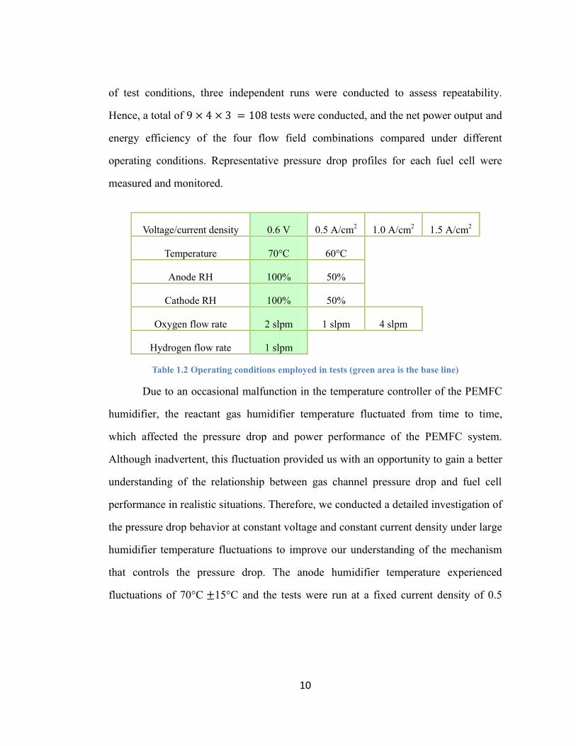
10
of test conditions, three independent runs were conducted to assess repeatability.
Hence, a total of 9 × 4 × 3 = 108 tests were conducted, and the net power output and
energy efficiency of the four flow field combinations compared under different
operating conditions. Representative pressure drop profiles for each fuel cell were
measured and monitored.
Voltage/current density 0.6 V 0.5 A/cm2 1.0 A/cm
2 1.5 A/cm
2
Temperature 70°C 60°C
Anode RH 100% 50%
Cathode RH 100% 50%
Oxygen flow rate 2 slpm 1 slpm 4 slpm
Hydrogen flow rate 1 slpm
Table 1.2 Operating conditions employed in tests (green area is the base line)
Due to an occasional malfunction in the temperature controller of the PEMFC
humidifier, the reactant gas humidifier temperature fluctuated from time to time,
which affected the pressure drop and power performance of the PEMFC system.
Although inadvertent, this fluctuation provided us with an opportunity to gain a better
understanding of the relationship between gas channel pressure drop and fuel cell
performance in realistic situations. Therefore, we conducted a detailed investigation of
the pressure drop behavior at constant voltage and constant current density under large
humidifier temperature fluctuations to improve our understanding of the mechanism
that controls the pressure drop. The anode humidifier temperature experienced
fluctuations of 70°C ±15°C and the tests were run at a fixed current density of 0.5

11
A/cm2 or a fixed voltage of 0.6 V for 30 minutes for each cell. All other operating
conditions were set to the baseline conditions as listed in Table 1.2.
1.4 Thesis Overview
The goal of this study is to improve the net power output of a PEM fuel cell by
employing different channel layouts on the anode and cathode sides. Net power output
will be compared for all four permutations of serpentine and interdigitated flow fields
on the cathode and anode sides, for different operating temperatures and relative
humidities. Chapter 1 described the background and motivation for this work along
with the objectives. A description of the experimental setup and fuel cell test
procedure is given in Chapter 2. The representative results showing pressure drop,
parasitic loss and net power output for fuel cells with different flow field layouts are
presented and discussed in Chapter 3. The influence of various operating conditions
such as temperature, oxygen flow rate and relative humidity on pressure drop and
power output is also presented in Chapter 3. The relationship between operating
conditions and energy efficiency for each flow field combination is also discussed.
Chapter 4 presents the correlation between fuel cell output and anode pressure drop
under large fluctuations in humidifier temperature, and investigates the mechanism
behind this correlation. Chapter 5 summarizes the major findings of this thesis, and
suggests potential future work.

12
Chapter 2
EXPERIMENTAL SETUP AND TEST PROCEDURE
2.1 Fuel Cell Components and Design
The objective of this thesis is to measure the net power output from fuel cells
employing different combinations of flow fields on the anode and cathode side. A total
of four combinations as listed in Table 1.1 were investigated. Accordingly, serpentine
and interdigitated flow field plates were designed and fabricated. The flow field
channels are 0.1016 cm (0.04 inch) wide × 0.1016 cm high (0.04 inch) × 5.0038 cm
long (0.5 inch) with a 0.0686 cm land width separating the channels in both flow
field plates, as shown in Fig. 2.1. The active area of each flow field is 25 cm2. The
flow field plates are made of 1.27 cm thick gold-coated aluminum 6061-T6. Other
associated components include end plates (2.5 cm thick Al 6061-T6) and current
collectors (0.2 cm thick gold plated aluminum).
Each end plate has one 180 W, 10 cm long embedded heater. A thermocouple
is bonded to the cathode end plate to control the cell temperature to within ±2°C of
the set value.
13
Figure 2.1 Schematics of interdigitated and single serpentine flow field designs built and tested in
this work
Identical membrane-electrode assemblies (MEAs) were used in all tests, and
each was comprised of a 5 cm × 5 cm Nafion NRE212 membrane (50μm thick)
sandwiched between two sheets of catalyst-coated gas diffusion electrodes (GDE)
loaded with 0.5 mg/cm2 Pt (purchased from FuelCellsEtc). The MEAs were fabricated
by hot-pressing the Nafion membrane between the two GDEs at 130°C for 2 minutes.
2.2 Fuel Cell Test Station
An Arbin fuel cell test stand was used to test the performance of all the flow
field combinations as shown in Figs. 2.2 and 2.3. The electronic load, flow rate,
temperature, humidity and back pressure were controlled and monitored by the test
stand at a sampling rate of 1 Hz. All tests were conducted with constant flow rates. For
our baseline operating condition, reactant gases were supplied at 70°C and 100% RH
with H2/O2 flow rates of 1/2 slpm, respectively.

14
Figure 2.2 Details of the Arbin fuel cell test stand
2.3 Pressure Measurement Station
Pressure drop across the cathode and anode sides of the cell are measured
using four Honeywell pressure sensors – 24PCDFA6A (14-200 kPa, accuracy 0.5% of
the full range) connected to the cell’s gas inlets and outlets, as shown in Fig. 2.3. The
data were recorded by a National Instruments DAQ board, which served as an
interface between the pressure sensors and a computer with LabVIEW, at a sampling
rate of 1 Hz. All pressure sensors were calibrated using a water-filled burette as shown
in Fig. 2.4 before testing.
15
Figure 2.3 Schematic of connection the four pressure sensors to the cell.
Figure 2.4 Use of a water-filled burette to calibrate the pressure sensors using a Labview program

16
2.4 Test Procedure
For each fuel cell with different combinations of flow fields as listed in Table
1.1, data were collected from cell tests. Test stand data (voltage, current density, cell
temperature, humidifier temperature, reactant gas temperatures, and gas mass flow
rates) and pressure differentials across the cathode and anode sides of the cell were
recorded simultaneously for each test. Each test run measured current data at a fixed
voltage, or voltage data at a fixed current for 30 minutes for the nine different
operating conditions listed in Table 1.2. Performance and pressure drop data were
plotted separately for each test and presented using the same time line. However,
Chapter 4 includes some plots which contain performance data overlaid with pressure
drop data to study the correlation between pressure drop and cell performance.
2.5 Summary
This chapter presented materials and dimensions of fuel cell components and
schematics of flow fields designs employed in this study. Details of the fuel cell test
stand and pressure measurement station used in the tests were also described. Baseline
operating conditions were described, as well as the methods used to collect and
present fuel cell test stand data and pressure differential data.

17
Chapter 3
RESULTS OF NET POWER WITH DIFFERENT FLOW FIELD
COMBINATIONS
3.1 Pressure Drop in Four Flow Fields Combinations
In most previous studies, researchers measured only the gross power from the
fuel cell but not the net power. Net power is gross power minus parasitic losses, which
are mainly due to the power required to pump air through the cathode flow field.
Pumping losses can be estimated by measuring the pressure drop across the flow fields
when conducting tests with the Arbin test stands. Experiments were conducted using
four flow field combinations as listed in Table 1.1 and cell performance and pressure
drops were recorded during testing. Net power was subsequently determined using the
pressure drop and cell performance data.
Cell performance and pressure drop behavior were recorded simultaneously
after stepping down to a constant voltage 0.6 V from open circuit, and tests were run
at standard operating conditions shown in Table 3.1. Current density fluctuated in a
small range when the cell was operated at fixed voltage as shown in the following
sections. Here, we chose 0.6 V because this is the voltage at which the cell can give a
high and steady gross power output. Prior to the test, the cell was operated at OCV for
30 minutes to preclude flooding, and thus the pressure drop and performance data
were not influenced by flooding at the beginning of the test. The test duration was set
to 30 minutes in order to provide adequate time to observe the occurrence of flooding
in the flow channels and any subsequent recovery.
18
Figure 3.1 shows the anode and cathode pressure differential profile in the four
types of cells tested. In the case of the ASCS cell, the average pressure drop was
around 28 kPa on the cathode side, and less than 10 kPa on the anode side. For the
AICI cell, the average pressure drop is around 12 kPa on the cathode side and 1 kPa
on the anode side. These values are reasonable because the gas flow velocities and
Reynolds number are much lower in the interdigitated flow field than those in the
serpentine flow field. Here, the gas flow velocity is defined at the inlet of each
channel, not at the inlet of the bipolar plates. Since the interdigitated flow field
contained 16 channels, the cross sectional area available for gas flow will be 16 times
higher than the cross sectional area in the single-serpentine channel, so the flow
velocity in each interdigitated channel will be proportionally lower [7]. In the case of
the AICS cell (Table 1.1), the average pressure drop in the interdigitated flow field
(anode) is close to the pressure drop in the anode side of the AICI cell, and the average
pressure drop in the ASCS flow field (cathode) is close to that in the cathode side of
the ASCS cell. In the case of the ASCI cell (Table 1.1), the average pressure drop in
each flow field is also close to that in the corresponding flow field in the ASCS and
AICI cells.
In Fig. 3.2, Fig. 3.3, Fig. 3.4 and Fig. 3.5, pressure drop curves in anode and
cathode flow fields were given for the four types of cells discharged at standard
operating condition for 30 minutes respectively. Fig. 3.2 shows the pressure drop
curves in ASCS cell, Fig. 3.3 shows the pressure drop curves in ASCI cell, Fig. 3.4
shows the pressure drop curves in AICS cell and Fig. 3.5 shows the pressure drop
curves in AICI cell. It is observed that the pressure drop on the anode side is always
lower than that on the cathode side even when the flow fields on both sides are the
19
same because the anode gas flow rate is only a half of the cathode flow rate. Second, it
is observed that the pressure drop sometimes increases after the fuel cell had been in
operation for a while, which is a sign of liquid water accumulation in channels. Liquid
water accumulation in the form of drops and slugs can block the gas channel, reducing
the cross sectional flow area of the gas channels, leading to a higher pressure drop
according to Darcy’s law. Third, water is produced at the cathode, so liquid water is
more likely to form on the cathode side in the cells; this could also contribute to the
higher pressure drop observed on the cathode side for each flow field combination.
Figure 3.1 Average pressure drop in each flow field during discharge at 0.6 V under standard
operating conditions for 30 minutes
20
Figure 3.2 Pressure drop profile in ASCS flow field during discharge at 0.6 V under standard
operating conditions for 30 minutes
Figure 3.3 Pressure drop profile in ASCI flow field during discharge at 0.6 V under standard
operating conditions for 30 minutes

21
Figure 3.4 Pressure drop profile in AICS flow field during discharge at 0.6 V under standard
operating conditions for 30 minutes
Figure 3.5 Pressure drop profile in AICI flow field during discharge at 0.6 V under standard
operating conditions for 30 minutes
22
3.2 Effect of Operating Conditions on Pressure Drop
As stated in Section 1.3, besides the standard operating conditions, eight
additional operating conditions listed in Table 1.2 were applied to each cell with the
four different flow field combinations. The influence of oxygen flow rate, cell
temperature, relative humidity, and current density on pressure drop is presented next.
Figure 3.6 Pressure drop in AICS cell at oxygen flow rates of 1, 2, and 4 slpm
Figure 3.6 shows the influence of oxygen flow rate on the cathode pressure
drop. Here, the pressure drop was monitored at 1 Hz, and the average pressure drop
was calculated over the full test duration of 30 minutes. In each flow field, we see that
cathode pressure drop is nearly proportional to the oxygen mass flow rate, which is
consistent with Eq.1.3. Figures 3.7 and 3.8 show the pressure drop curves for the
AICS cell at different oxygen flow rates. We can see that the average cathode pressure
drop is about 14kPa in when oxygen flow rate is1 slpm and about 73kPa when oxygen
flow rate is 4 slpm, which indicates that oxygen flow rate has a major impact on
cathode pressure drop in flow fields.
23
Figure 3.7 Pressure drop profile in AICS flow field during discharge at 0.6V and oxygen flow rate
1 slpm for 30 minutes
Figure 3.8 Pressure drop profile in AICS flow field during discharge at 0.6V and oxygen flow rate
of 4 slpm for 30 minutes

24
Figure 3.9 Average pressure drop in each flow field during discharge at 0.6 V for 30 minutes at
60°C and 70°C
Figure 3.9 shows that the pressure drop reduces slightly when the temperature
is reduced to 60°C. From the performance profiles in the following sections, we will
see that the current density for 0.6 V at 60°C is lower than that at 70°C. A lower
current density means that the reaction rate is lower, implying a lower water
production rate and a lower propensity for water flooding. Hence, the pressure drop
can be expected to reduce when the current density decreases.
25
Figure 3.10 Average pressure drop in each flow field during discharge at 0.6 V for 30 minutes at
50% cathode RH 100% cathode RH
Figure 3.10 compares the cathode pressure drop for cathode RH levels of 50%
and 100%. The cathode pressure drop at 50% RH is always lower than that for 100%
RH. This is to be expected because a lower RH decreases the propensity for flooding.
Moreover, lower RH in the inlet gas flow may cause membrane dryout leading to low
protonic conductivity of membrane, and thus higher ohmic losses. For a fixed
operating voltage, higher ohmic losses will result in a reduced current density, which
means a lower reaction rate. As explained above, a lower reaction rate implies water
production rates, leading to a smaller pressure drop in the cathode gas channels.
26
Figure 3.11 Average pressure drop in each flow field during discharge at 0.5, 1, and 1.5 A/cm
2 for
30 minutes
Next, the fuel cell was operated at a fixed current density (0.5, 1, and 1.5
A/cm2) instead of a fixed voltage for 30 minutes to study the effect of current density
on pressure drop and net power in the different flow field combinations. For a fixed
current density, the cell voltage fluctuates slightly as shown in the performance curves.
As shown in Fig. 3.11, the pressure drop increases with current density for the same
reasons as presented earlier.
3.3 Parasitic Power Loss Calculation and Net Power
In the preceding sections, the measured voltage and current density data
provided the gross power produced by the cell. In order to obtain the net power, the
parasitic power losses must be subtracted from the gross power. Usually, compressor
power is the major contributor to the parasitic losses in a fuel cell system, so we
assumed that the entire parasitic loss can be equated to the power consumed by the
compressor to drive air through the cathode flow field [11]. Anode pumping losses are

27
ignored since in most applications the hydrogen is supplied from a high pressure tank
without the need of a pump. Compressor power is evaluated as follows [5]:
𝑃compressor = 𝑐𝑝𝑇1
𝜂𝑚𝜂𝑐�̇� [(
𝑝2
𝑝1)
𝛾−1
𝛾− 1] 3.1
where 𝑇1 is the inlet temperature (in K), 𝑐𝑝 is the specific heat capacity at constant
pressure (in J/kg-K), 𝑝1 is atmosphere pressure, 𝑝2 is inlet pressure, �̇� is the gas mass
flow rate (in kg/s), 𝜂𝑐 is the compressor efficiency, 𝜂𝑚 is the motor efficiency, and 𝛾
is the ratio of specific heat capacities, 𝑐𝑝/𝑐𝑣 . Here we use values for oxygen at
standard conditions: 𝑝1 = 100 kPa, 𝑇1 = 293 K, 𝑐𝑝 = 0.918 kJ/kg-K, 𝛾 = 1.40, and
typical values for efficiencies: 𝜂𝑐 = 0.7 and 𝜂𝑚 = 0.9. An oxygen flow rate of 2 slpm
at 1.33 kg/m3 gives a mass flow rate of 4.43 × 10⁻⁵ kg/s [5].
Equation 3.1 was used to calculate the compressor power by inserting the
measured value of 𝑝2 for each cell discharging at either constant voltage or constant
current density for 30 minutes. The net power for each test was obtained as the
difference between the measured gross power output and the calculated parasitic
power loss.
Three tests were conducted for each operating condition and we report the
average value for the measured performance and pressure drop. We also calculated the
standard deviation and examined the confidence level from an ANOVA analysis. If the
standard deviation exceeds the difference between the mean values of net power
output, then it cannot be guaranteed that the differences within the same test group can
be ignored compared to the differences across different test groups. As shown in Fig.
3.12, the ASCI fuel cell has the highest net power output for the four flow field
combinations at standard operating conditions due to the lower pressure drop on the
cathode side, and hence lower parasitic loss. The values of standard deviation

28
presented in Fig. 3.13 show that the variations in net power within the same test group
are much too small to affect our conclusions.
Figure 3.12 Average total power output, parasitic power loss and net power in each cell; cells were
operated at standard operating conditions for 30 minutes at 0.6 V. Net power is defined as the
difference between total power output and parasitic power loss. The quoted values are in watts.
Figure 3.13 Average net power in each cell; cells were operated at standard operating condition
for 30 minutes at 0.6 V. Standard deviations were calculated from three tests for total power
output and parasitic loss to assess variations in test results within the same group of experiments.
Since we have three tests for each flow field at the same operating condition, to
ensure that the difference in net power of different cells is significant and our

29
conclusions are robust, we conducted an ANOVA test for four flow field combinations
in each test group.
Since we have three tests for each flow field at the same operating condition, to
ensure that the difference in net power of different cells is significant and our
conclusions are robust, we conducted an ANOVA test for two groups of test results
corresponding to the flow fields exhibiting the better results: the ASCI and ASCS
cells. Here we set the confidence limit as 95%; so when the p-value of the ANOVA
test is smaller than 0.05, the null hypothesis (the mean values of data groups are equal)
will be rejected, and we can conclude that there is a significant difference between
groups. Conversely, when the p-value of the ANOVA test exceeds 0.05, we cannot
conclude that there is a significant difference between groups. The p-values of the
ANOVA tests for each case are summarized in Table 3.1. All the p-values calculated
by the ANOVA analysis for all the test groups were smaller than 0.05 which confirms
that our conclusions regarding which flow field has the better net power output are
robust.
Operating condition p-value
0.6 V 0.0001
0.5 A/cm2 0.0016
1 A/cm2 0.0018
1.5 A/cm2 0.002
anode RH 50% 0.016
cathode RH 50% 0.0003
oxygen flow rate 1 slpm 0.018
oxygen flow rate 4 slpm 3.12E-5
60°C 0.001
Table 3.1 P-values for the net power results for the ASCI and ASCS flow fields at each specific
operating condition
30
3.4 Power Efficiency Discussion
Figure 3.14 Power efficiency of each flow field at standard operation conditions at 0.6 V
An example of energy efficiency evaluation is shown in Fig. 3.14 by
calculating the fraction of parasitic losses for all cell combinations discharging at 0.6
V under standard operating conditions. We noticed that parasitic losses can be as large
42% of the total power output. The energy efficiency of the ASCI cell is the highest of
all the four cells, whereas the AICS cell has the lowest energy efficiency.
3.5 Effect of Operating Conditions on Net Power Output and Power Efficiency
One specific operating parameter is changed at a time to investigate the net
power output of four cells under various operating conditions. As described earlier, the
influence of relative humidity on each side, temperature, current density, and oxygen
31
flow rate on the net power of each cell was investigated, and three tests were
conducted for each condition to ensure repeatability.
From Eq.3.1, we see that parasitic losses should double if we double the
oxygen flow rate. However, the performance of the fuel cell will also improve when
the oxygen flowc rate increases because of lower concentration losses. Performance
and pressure drop were measured for each cell, and the net power was calculated and
compared in Fig. 3.15. As shown, the ASCI cell has the best net power output among
the four cells, and the difference between it and the other cells exceeds the calculated
standard deviations. It can also be seen that the AICI cell exhibits a better net power
output than the ASCS cell because of the large parasitic losses experienced by the
ASCS cell at large gas flow rates.
Figure 3.15 Average total power output, parasitic power loss and net power in each cell; oxygen
flow rate was 4 slpm and other conditions remain the same. Cells were operated for 30 minutes at
0.6 V.
Energy efficiency at high oxygen flow rates were also calculated for the four
cells. From Fig. 3.16, we see that the energy efficiency at a high oxygen flow rate (4
slpm) is much lower than that at the standard oxygen flow rate (2 slpm). In particular,
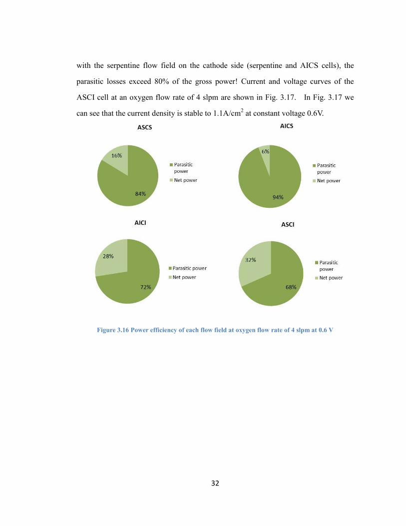
32
with the serpentine flow field on the cathode side (serpentine and AICS cells), the
parasitic losses exceed 80% of the gross power! Current and voltage curves of the
ASCI cell at an oxygen flow rate of 4 slpm are shown in Fig. 3.17. In Fig. 3.17 we
can see that the current density is stable to 1.1A/cm2 at constant voltage 0.6V.
Figure 3.16 Power efficiency of each flow field at oxygen flow rate of 4 slpm at 0.6 V

33
Figure 3.17 Current density and voltage profile of ASCI cell during discharge at 0.6V and oxygen
flow rate of 4 slpm for 30 minutes
The net power of the four cells at the low oxygen flow rate of 1 slpm is shown
in Fig. 3.18. We note that the gross power output for each cell drops significantly
compared with the gross power output at high oxygen flow rates due to increased mass
transport losses; however, the parasitic loss at the low gas flow rate is also much
lower. Therefore, the net power at 1 slpm oxygen flow rate is still higher than the net
power at 4 slpm because of the large parasitic losses at this highest oxygen flow rate;
however, it is not better than the net power at the oxygen flow rate of 2 slpm. From the
above comparison we can see that there is a trade-off between high gross performance
and high power losses when the oxygen flow rate is changed. We also see that the
ASCI cell still has the best net power amongst the four cells; however, the difference
of the net power between cells is much smaller, and is probably not significant if we
take the standard deviation into consideration. According to the p-values in Table 3.1

34
for this test group, there is still a significant difference between the net power results
of different cells since the p-value is smaller than 0.05.
Figure 3.18 Average total power output, parasitic power loss and net power in each cell; oxygen
flow rate was 1 slpm and other conditions remain the same. Cells were operated for 30 minutes at
0.6 V.
Figure 3.19 shows the energy efficiency of each cell at the oxygen flow rate of
1 slpm. Compared with Fig. 3.16 it is clear that the energy efficiency at this lowest
oxygen flow rate is higher, about 75% for each cell. This could be easily understood
through Eq.3.1 that a low gas flow rate should result in a small parasitic power loss.
Current density and voltage curves of the ASCI cell at an oxygen flow rate of 1 slpm
are shown in Fig. 3.20. In Fig.3.20 we see that current density is steady around
0.71A/cm2, which is much smaller than it in Fig.3.17 since lower oxygen flow rate can
affect reaction rate at the electrodes.

35
Figure 3.19 Power efficiency of each flow field at oxygen flow rate of 1 slpm at 0.6 V
Figure 3.20 Current density and voltage profile of ASCI cell during discharge at 0.6V and oxygen
flow rate of 1 slpm for 30 minutes
36
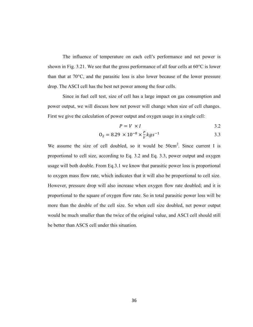
The influence of temperature on each cell’s performance and net power is
shown in Fig. 3.21. We see that the gross performance of all four cells at 60°C is lower
than that at 70°C, and the parasitic loss is also lower because of the lower pressure
drop. The ASCI cell has the best net power among the four cells.
Since in fuel cell test, size of cell has a large impact on gas consumption and
power output, we will discuss how net power will change when size of cell changes.
First we give the calculation of power output and oxygen usage in a single cell:
𝑃 = 𝑉 × 𝐼 3.2
O2 = 8.29 × 10⁻⁸ ×𝑃
𝑉𝑘𝑔𝑠−1 3.3
We assume the size of cell doubled, so it would be 50cm2. Since current I is
proportional to cell size, according to Eq. 3.2 and Eq. 3.3, power output and oxygen
usage will both double. From Eq.3.1 we know that parasitic power loss is proportional
to oxygen mass flow rate, which indicates that it will also be proportional to cell size.
However, pressure drop will also increase when oxygen flow rate doubled; and it is
proportional to the square of oxygen flow rate. So in total parasitic power loss will be
more than the double of the cell size. So when cell size doubled, net power output
would be much smaller than the twice of the original value, and ASCI cell should still
be better than ASCS cell under this situation.
37
Figure 3.21 Average total power output, parasitic power loss and net power in each cell; cell
temperature was 60°C and other conditions remain the same. Cells were operated for 30 minutes
at 0.6 V.
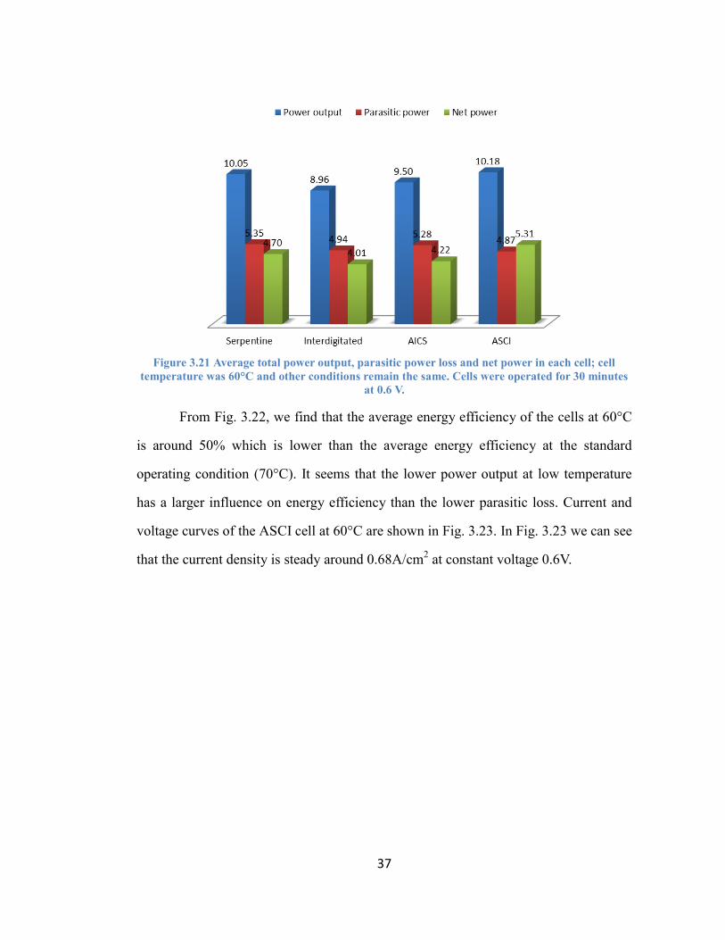
From Fig. 3.22, we find that the average energy efficiency of the cells at 60°C
is around 50% which is lower than the average energy efficiency at the standard
operating condition (70°C). It seems that the lower power output at low temperature
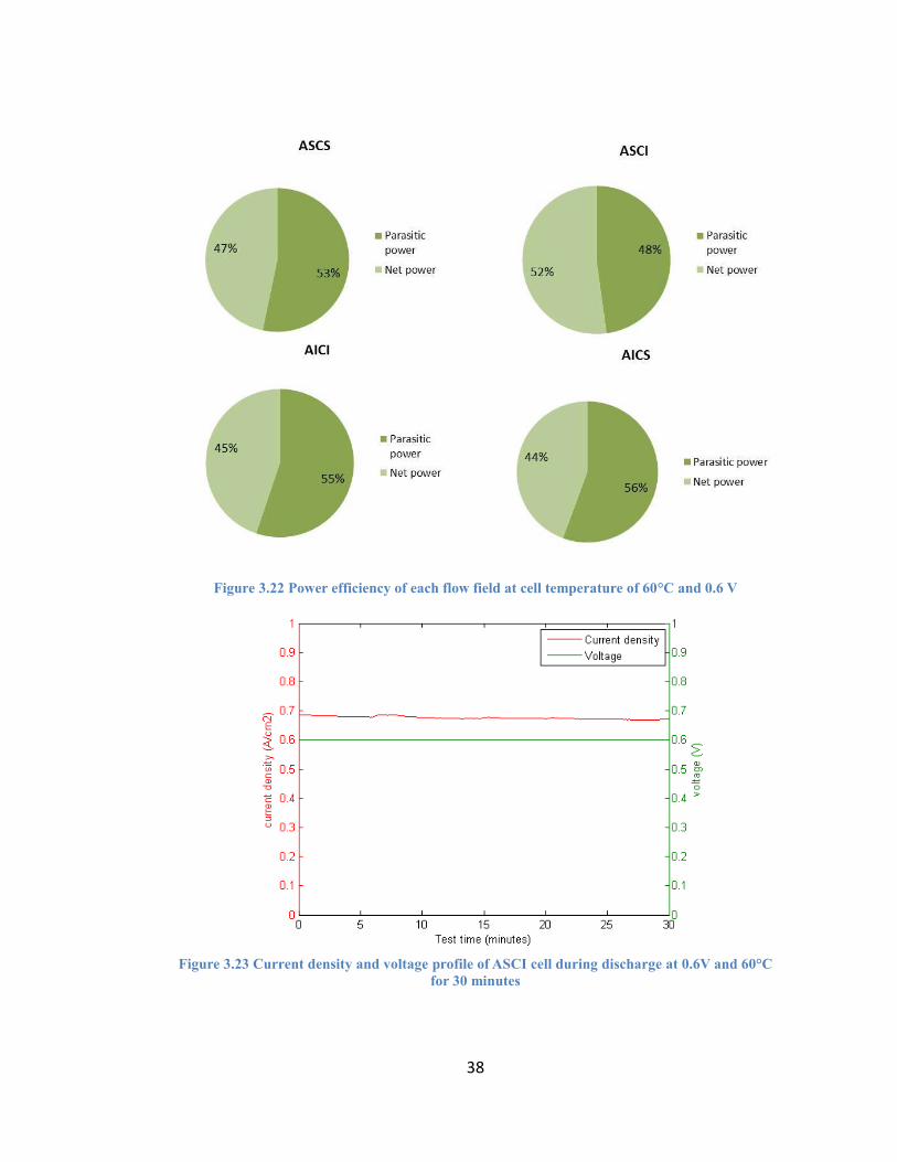
has a larger influence on energy efficiency than the lower parasitic loss. Current and
voltage curves of the ASCI cell at 60°C are shown in Fig. 3.23. In Fig. 3.23 we can see
that the current density is steady around 0.68A/cm2 at constant voltage 0.6V.
38
Figure 3.22 Power efficiency of each flow field at cell temperature of 60°C and 0.6 V
Figure 3.23 Current density and voltage profile of ASCI cell during discharge at 0.6V and 60°C
for 30 minutes
39
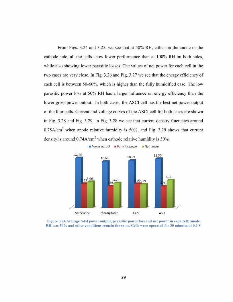
From Figs. 3.24 and 3.25, we see that at 50% RH, either on the anode or the
cathode side, all the cells show lower performance than at 100% RH on both sides,
while also showing lower parasitic losses. The values of net power for each cell in the
two cases are very close. In Fig. 3.26 and Fig. 3.27 we see that the energy efficiency of
each cell is between 50-60%, which is higher than the fully humidified case. The low
parasitic power loss at 50% RH has a larger influence on energy efficiency than the
lower gross power output. In both cases, the ASCI cell has the best net power output
of the four cells. Current and voltage curves of the ASCI cell for both cases are shown
in Fig. 3.28 and Fig. 3.29. In Fig. 3.28 we see that current density fluctuates around
0.75A/cm2 when anode relative humidity is 50%, and Fig. 3.29 shows that current
density is around 0.74A/cm2 when cathode relative humidity is 50%.
Figure 3.24 Average total power output, parasitic power loss and net power in each cell; anode
RH was 50% and other conditions remain the same. Cells were operated for 30 minutes at 0.6 V

40
Figure 3.25 Average total power output, parasitic power loss and net power in each cell; cathode
RH was 50% and other conditions remain the same. Cells were operated for 30 minutes at 0.6 V.
Figure 3.26 Power efficiency of each flow field at anode RH 50% and 0.6 V

41
Figure 3.27 Power efficiency of each flow field at cathode RH 50% and 0.6 V
Figure 3.28 Current density and voltage profile of ASCI cell during discharge at 0.6V and anode
RH 50% for 30 minutes
42
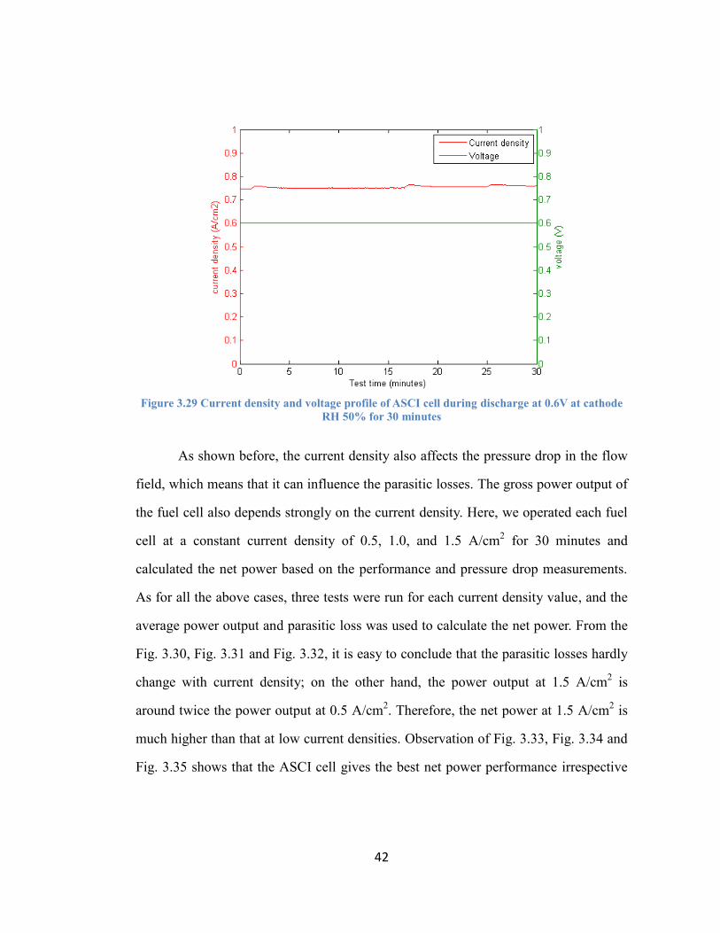
Figure 3.29 Current density and voltage profile of ASCI cell during discharge at 0.6V at cathode
RH 50% for 30 minutes
As shown before, the current density also affects the pressure drop in the flow
field, which means that it can influence the parasitic losses. The gross power output of
the fuel cell also depends strongly on the current density. Here, we operated each fuel
cell at a constant current density of 0.5, 1.0, and 1.5 A/cm2 for 30 minutes and
calculated the net power based on the performance and pressure drop measurements.
As for all the above cases, three tests were run for each current density value, and the
average power output and parasitic loss was used to calculate the net power. From the
Fig. 3.30, Fig. 3.31 and Fig. 3.32, it is easy to conclude that the parasitic losses hardly
change with current density; on the other hand, the power output at 1.5 A/cm2 is
around twice the power output at 0.5 A/cm2. Therefore, the net power at 1.5 A/cm
2 is
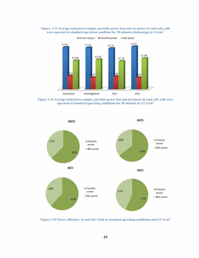
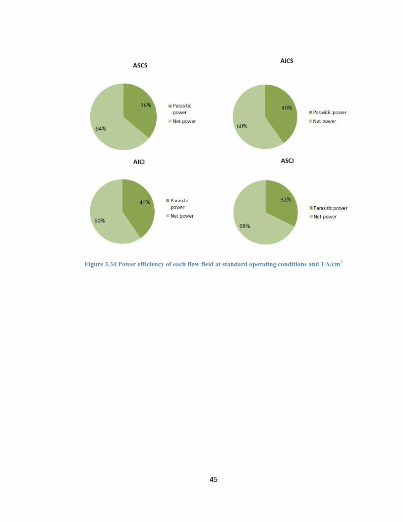
much higher than that at low current densities. Observation of Fig. 3.33, Fig. 3.34 and
Fig. 3.35 shows that the ASCI cell gives the best net power performance irrespective
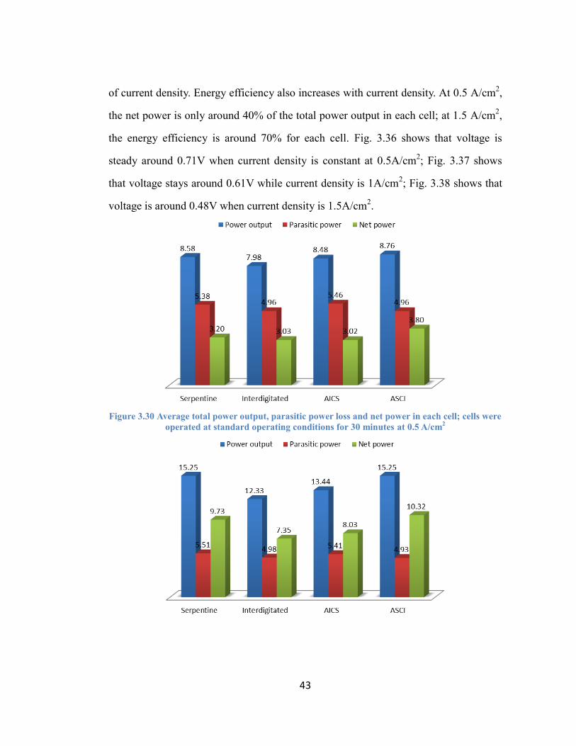
43
of current density. Energy efficiency also increases with current density. At 0.5 A/cm2,
the net power is only around 40% of the total power output in each cell; at 1.5 A/cm2,
the energy efficiency is around 70% for each cell. Fig. 3.36 shows that voltage is
steady around 0.71V when current density is constant at 0.5A/cm2; Fig. 3.37 shows
that voltage stays around 0.61V while current density is 1A/cm2; Fig. 3.38 shows that
voltage is around 0.48V when current density is 1.5A/cm2.
Figure 3.30 Average total power output, parasitic power loss and net power in each cell; cells were
operated at standard operating conditions for 30 minutes at 0.5 A/cm2
44
Figure. 3.31 Average total power output, parasitic power loss and net power in each cell; cells
were operated at standard operation condition for 30 minutes discharging at 1A/cm2.
Figure 3.32 Average total power output, parasitic power loss and net power in each cell; cells were
operated at standard operating conditions for 30 minutes at 1.5 A/cm2
Figure 3.33 Power efficiency of each flow field at standard operating conditions and 0.5 A/cm
2
45
Figure 3.34 Power efficiency of each flow field at standard operating conditions and 1 A/cm
2

46
Figure 3.35 Power efficiency of each flow field at standard operating conditions and 1.5 A/cm
2
47
Figure 3.36 Current density and voltage profile of ASCI cell during discharge at 0.5A/cm
2 for 30
minutes
Figure 3.37 Current density and voltage profile of ASCI cell during discharge at 1A/cm
2 for 30
minutes
48
Figure 3.38 Current density and voltage profile of ASCI cell during discharge at 1.5A/cm
2 for 30
minutes
3.6 Summary
In this chapter, pressure drop data for four flow field combinations was
presented and compared, and the effect of operating conditions on pressure drop
was also discussed. It was found that the pressure drop in the interdigitated flow
field was usually much lower than that in the serpentine flow field. It was also
shown that the pressure drop is nearly proportional to the gas flow rate in the
same flow field when other operating conditions are the same. The pressure drop
at an operating temperature of 60°C is lower than that at 70°C. Lower relative
humidity at either anode or cathode can also result in a lower pressure drop. In
addition, high current densities can cause a higher pressure drop in the same flow
field when all the other operating conditions are the same.
Also presented in this chapter were gross power output, parasitic power
loss, and net power output for each flow field combination and each set of

49
operating conditions. The effect of operating condition on energy efficiency of
each cell was also discussed. The ASCI cell always gave the best net power
output for all operating conditions due to high gross power and low parasitic
loss. We also found that a lower oxygen flow rate can give higher energy
efficiency than a higher gas flow rate. The current density of 1.5A/cm2 leads to
higher energy efficiency than the current density 0.5A/cm2. However, the
influence of relative humidity and operating temperature on energy efficiency is
not as significant as current density and oxygen flow rate.

50
Chapter 4
PRESSURE DROP BEHAVIOR IN PEM FUEL CELLS UNDER
FLUCTUATING HUMIDIFICATION TEMPERATURES
4.1 Correlation Between Fuel Cell Voltage and Anode Pressure Drop
During fuel cell operation in automotive, portable and stationary applications,
the operating temperature and relative humidity could fluctuate due to imperfections in
design or minor disturbances in the cooling system or other auxiliary systems. To
understand the effect of temperature fluctuations on fuel cell performance and pressure
drop behavior, we exploited fluctuations in the humidification temperature of ± 20°C
around the set point of 70°C. Figure 4.1 shows the typical pressure drop profiles under
such humidification temperature fluctuations. In contrast with the stable pressure drop
profiles presented in the section 3.1 wherein the humidification temperature was
stable, it is observed that the pressure drop profile in Fig. 4.1 undergoes large
fluctuations.
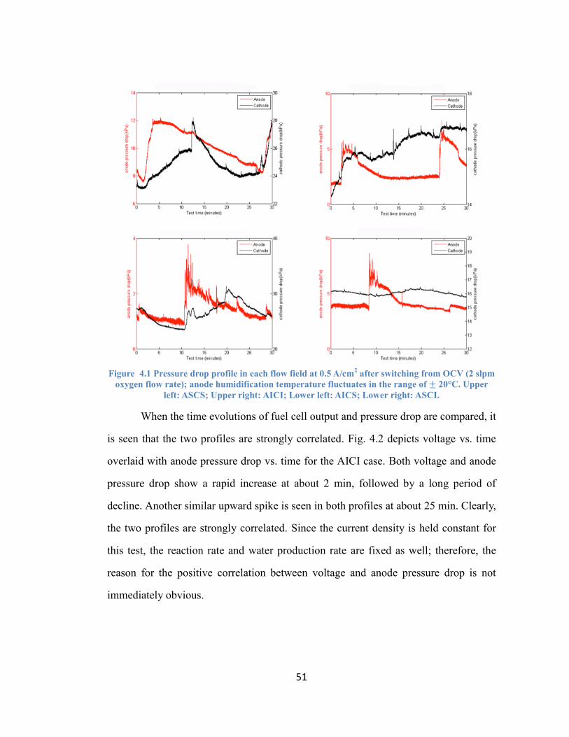
51
Figure 4.1 Pressure drop profile in each flow field at 0.5 A/cm
2 after switching from OCV (2 slpm
oxygen flow rate); anode humidification temperature fluctuates in the range of ± 20°C. Upper
left: ASCS; Upper right: AICI; Lower left: AICS; Lower right: ASCI.
When the time evolutions of fuel cell output and pressure drop are compared, it
is seen that the two profiles are strongly correlated. Fig. 4.2 depicts voltage vs. time
overlaid with anode pressure drop vs. time for the AICI case. Both voltage and anode
pressure drop show a rapid increase at about 2 min, followed by a long period of
decline. Another similar upward spike is seen in both profiles at about 25 min. Clearly,
the two profiles are strongly correlated. Since the current density is held constant for
this test, the reaction rate and water production rate are fixed as well; therefore, the
reason for the positive correlation between voltage and anode pressure drop is not
immediately obvious.

52
Figure 4.2 AICI cell test at 0.5 A/cm
2. Upper left: fuel cell performance data; lower left: anode
and cathode pressure drop; right: anode pressure drop and voltage data

53
Figure 4.3 AICI cell test at 0.5 A/cm
2. Upper: time evolution over 30 min of current density
overlaid with the anode pressure drop. The other two sub-plots are close-up views of the two
spikes over a narrow time span.
To understand the mechanism behind this correlation, we take a closer look at
the two profiles in the vicinity of the spikes over a narrow time span of 50 s. In Fig.
4.3, we see that at the first voltage spike commences at 131 s, and the anode pressure
drop responds after a slight delay at 138 s. Similarly, at the second spike, the voltage
begins to rise at 1430 s, followed by the pressure drop’s response at 1445s. The
voltage and anode pressure drop profiles were examined for fuel cells with the other
flow field combinations as well, and it was noticed that the spike in the pressure drop
always followed the voltage spike after a short delay.
Since the water production rate was held constant for these tests, the rise in the
anode pressure drop must be due to water buildup in the anode channel. At the same

54
time, the rise in voltage must be due to a sudden drop in voltage losses. Since internal
current and activation losses are less likely to change for the given cell temperature,
the most likely scenario is that the ohmic loss was decreased by a sudden
improvement in the membrane’s proton conductivity. We examined the anode
humidifier temperature profile for the same time period from the test datasheet, and
investigated the possible influence of humidifier temperature on fuel cell voltage. Fig.
4.4 shows that the cell voltage increased shortly after the hydrogen humidifier
temperature spiked, and then decreased after the humidifier temperature dropped.
Since the fuel cell was operated at open circuit for 30 min before discharging at 0.5
A/cm2, the membrane might initially be in a relatively dry condition. Due to a spike in
the humidifier temperature, the anode RH would rise rapidly improving the
membrane’s hydration level, and consequently, its proton conductivity. Thus, a spike
in the anode humidifier temperature leads to a drop in the ohmic voltage loss, and a
spike in the cell voltage. Higher anode RH would also lead to a higher likelihood of
liquid water condensation in the anode channels, which will cause a sudden rise in the
anode pressure drop. Therefore, we see a strong correlation between the cell voltage
and anode pressure drop. Furthermore, because the membrane is very thin, its rate of
hydration is quicker than the rate at which water vapor condenses and accumulates in
the gas flow channels, therefore the spike in the cell voltage slightly precedes the spike
in the anode pressure drop.

55
Figure 4.4 Humidification temperature and voltage data for the AICI cell at 0.5 A/cm
2 for 30
minutes

56
4.2 Correlation Between Fuel Cell Current Density and Pressure Drop
Figure 4.5 ASCI cell test at 0.6 V. Upper left: fuel cell performance data; lower left: anode and
cathode pressure drop; right: anode pressure drop and voltage data
Figure 4.5 depicts the current density overlaid with the anode pressure drop at
a fixed voltage of 0.6 V. The spikes in the current curve are strongly correlated with
the spikes in the pressure drop profile. As before, we focused on the data in the
vicinity of the spikes over a narrow time span of 50 s to investigate the mechanism
responsible for this correlation, as shown in Fig. 4.6.
As seen earlier for the case of constant current density where the voltage spikes
preceded the spikes in anode pressure drop, Fig. 4.6 shows that when the cell is
operated at constant voltage, the current spike precedes the spike in anode pressure
drop. It is reasonable that the spike in anode pressure drop is caused by a rise in the
water production rate, i.e. the reaction rate, which is proportional to the cell’s current

57
density. Therefore, it stands to reason that the pressure drop rise lags a few seconds
behind the sharp rise in current density. To investigate the reason for the spike in
current density, we examined the anode humidifier temperature vs. time profile. Fig.
4.7 shows that the two spikes in the hydrogen humidifier temperature correspond
closely to the two spikes in the current density curve; moreover, the rise in the
humidifier temperature is always followed a short time later by a rise in current
density. In fact, this behavior is identical to the one see earlier in Fig. 4.4. Fig. 4.7 also
shows that the sharp increase in current density at around 20 minutes is correlated with
an increase in the oxygen humidifier temperature. Higher humidifier temperature on
either the anode or the cathode can increase the RH within the cell leading to better
membrane hydration and reduced ohmic losses. Therefore, at a fixed cell voltage, a
reduction in ohmic losses has the effect of increasing the cell’s current. A higher
current implies a higher reaction rate, which means that the water production rate
increases. Higher relative humidity also can aggravate flooding within the flow field
channels. Considering the influence of both higher water production rate and higher
water content in the incoming gas flow, we can conclude that they together contribute
to the increase in the pressure drop; furthermore, it also explains why the rise in
pressure drop lags slightly behind the rise in current density.

58
Figure 4.6 ASCI cell test at 0.6 V. Upper left: time evolution over 30 min of current density
overlaid with the anode pressure drop. The other three sub-plots are close-up views of the three
spikes over a narrow time span.

59
Figure 4.7 Humidification temperature and voltage data for the ASCI cell at 0.6 V for 30 minutes
4.3 Correlation Coefficients
We calculated the correlation coefficients between the anode pressure drop and
cell output (voltage in the case of fixed current density, or current density in the case
of fixed voltage) for each test run at standard operating conditions. The results are
summarized in Fig. 4.8 and confirm that there is always a strong correlation between

60
anode pressure drop and cell output (correlation coefficient always exceeds 0.5).
Figure 4.8 Correlation coefficients of anode pressure drop and cell current density at 0.6 V
Figure 4.9 Correlation coefficients of anode pressure drop and cell voltage at 0.5A/cm
2
4.4 Discussion
From Fig.4.2 and Fig. 4.5, it is interesting to note that the correlation between
the anode pressure drop with fuel cell output is stronger than that between the cathode

61
pressure drop and cell output. For example, in Fig. 4.5, all the spikes in the current
curve correspond with the spikes in the anode pressure drop profile; however, a similar
correspondence is not evident for the cathode pressure drop profile. This could be due
to the fact that the anode humidifier temperature experienced larger fluctuations than
the cathode humidifier temperature. Consequently, the RH fluctuations on the anode
side are larger, leading to a higher propensity for flooding in the anode channels and
the associated rise in the anode pressure drop.
4.5 Summary
In this chapter, we exploited fluctuations in the humidifier temperature of
± 20°C around the set point of 70°C to understand the effect of temperature
fluctuations on fuel cell performance and pressure drop behavior. Positive correlation
between anode pressure drop and fuel cell output was found. We took a closer look at
the anode pressure drop and fuel cell output profiles in the vicinity of spikes over a
narrow time span of 50 s and found that the fuel cell power output spike precedes the
spike in anode pressure drop. By examining the humidifier temperature vs. time
profile, we found that spikes in the humidifier’s temperature raised the RH in the cell
and led to an increase in the membrane’s proton conductivity which reduced ohmic
losses. Consequently, fuel cell performance improved. At the same time, higher anode
RH also increases the likelihood of liquid water condensation in the anode channels.
This explains the positive correlation between fuel cell output and pressure drop.

62
Chapter 5
CONCLUSIONS AND FUTURE WORK
In this work, a novel asymmetric flow field combination design for PEMFCs
was presented and its effect on net power output was investigated. The two new flow
field combinations investigated here were anode-serpentine/cathode-interdigitated
(ASCI), and anode-interdigitated/cathode-serpentine (AICS), and their performance
was compared against conventional serpentine and interdigitated flow field designs.
Net power output was evaluated for PEMFCs with four sets of flow field combinations
using performance data and pressure drop data collected from test runs at constant
voltage or constant current. The pressure drop of each cell under different test
conditions was presented and compared. It was found that at high oxygen flow rate,
high humidity and high current density could cause a relatively high pressure drop,
and thus a large parasitic loss.
We also measured performance and pressure drop data for different sets of
operating conditions and calculated the net power output and energy efficiency for
each specific operating condition. Results show that the ASCI cell always has the best
net power output among the four types of flow fields across all operating conditions
tested due to a reasonably good performance combined with a small parasitic loss.
ANOVA analysis was conducted for all the calculated results to assess the relative
magnitude of random error in the experimental results. We also discussed the
influence of operating conditions on the energy efficiency of the cells; for example, a

63
reduced oxygen flow rate can help to improve the energy efficiency by reducing
parasitic losses significantly.
In conclusion, the new anode-serpentine/cathode-interdigitated PEMFC design
evaluated in this work can significantly improve the net power output of the PEMFC
system because of its low parasitic power losses, and offers a simple way to improve
the net performance of PEM fuel cells, making it more cost effective.
The mechanisms responsible for dynamic changes in the anode and cathode
pressure drops were also studied and discussed in this work; these studies led to a
better understanding of the electrochemical reaction rates and their impact on water
dynamics in the PEMFC. An increasing trend was found in some of the pressure drop
profiles; as operation time increases, water is produced, diffused and condensed
continuously inside the fuel cell, and the accumulation of liquid water in the gas
channel can result in an increase in the pressure drop.
Besides power analysis, we also investigated dynamic fluctuations in the
pressure drop and their relationship with fluctuations in the cell output and humidifier
temperature. We found that the pressure drop in the flow channels always showed a
positive correlation with the cell output; furthermore, the anode pressure drop was
more strongly correlated with cell output than the cathode pressure drop since only the
anode humidifier experienced large temperature fluctuations. The positive correlation
between cell output and pressure drop arises from the spikes in humidifier temperature
which raise the RH in the cell causing an increase in proton conductivity and reduced
ohmic losses. The positive correlation is even stronger when the cell is operated at
50% relative humidity. The above findings confirm that inlet gas humidity can play an
important role in PEM fuel cell operation due to its strong influence on proton
64
conductivity, reaction rate, liquid water dynamics, and compressor power
consumption. Therefore, it influences the overall performance and net power output of
the PEMFC system.
Due to limited time, in addition to the baseline value, we explored the
influence of cell temperature and relative humidity at one other value (temperature
60°C and RH 50%). Future work can examine the influence of temperature and RH by
conducting a systematic parametric study. For example, temperature can be varied
from 30°C to 90°C in 10°C increments to determine the effect of low and high
temperature on cell net power output for ASCI and AICS cells. Optimized operating
conditions for each flow field can also be studied in the future. Finally, all of the
studies presented here pertain to single cells; it would be useful to study how these
novel asymmetric flow field combinations would perform when employed within a
stack to assess energy savings.

65
REFERENCES
[1]Pukrushpan, J. T. (2003). Modeling and control of fuel cell systems and fuel
processors, Doctoral Dissertation, University of Michigan.
[2] Lee, H. J. (2009). Modeling and Analysis of a PEM Fuel Cell System for a
Quadruped Robot, Master of Science Thesis, Mechanical Engineering, Auburn
University
[3] Catlin, G. (2010). PEM fuel cell modeling and optimization using a genetic
algorithm, Master of Science Thesis, Mechanical Engineering, University of Delaware
[4] Wang, L., and Liu, H. (2004). Performance studies of PEM fuel cells with
interdigitated flow fields. Journal of Power Sources, 134(2), 185-196.
[5] Larminie, J., Dicks, A., and McDonald, M.S. Fuel cell systems explained, Second
Ed., John Wiley & Sons Ltd, Chichester, 2003.15
[6] Hermann, A., Chaudhuri, T., & Spagnol, P. (2005). Bipolar plates for PEM fuel
cells: A review. International Journal of Hydrogen Energy, 30(12), 1297-1302.
[7] Spernjak, D., Prasad, A. K., & Advani, S. G. (2010). In situ comparison of water
content and dynamics in parallel, single-serpentine, and interdigitated flow fields of

66
polymer electrolyte membrane fuel cells. Journal of Power Sources, 195(11), 3553-
3568.
[8] Kuo, J. K., Yen, T. S., & Chen, C. O. K. (2008). Improvement of performance of
gas flow channel in PEM fuel cells. Energy Conversion and Management,49(10),
2776-2787.
[9] Wang, L., Husar, A., Zhou, T., and Liu, H. (2003). A parametric study of PEM fuel
cell performances. International Journal of Hydrogen Energy, 28(11), 1263-1272.
[10] Barbir, F., Balasubramanian, B., and Neutzler, J. K. (1999). Trade-off design
study of operating pressure and temperature in PEM fuel cell systems. In 1999 ASME
International Mechanical Engineering Congress and Exposition.
[11] Barbir, F. (1999). Review of hydrogen conversion technologies. Hemijska
Industrija, 53(12), 426-433.
[12] Liu, X., et al. (2007). Water flooding and pressure drop characteristics in flow
channels of proton exchange membrane fuel cells. Electrochimica Acta 52(11): 3607-
3614.
[13] Spernjak, D. (2010). Experimental characterization of water transport in polymer
electrolyte fuel cells, Doctoral Dissertation, University of Delaware

67
[14] Bosco, A. D., and Fronk, M. H. (2000). U.S. Patent No. 6,103,409. Washington,
DC: U.S. Patent and Trademark Office.
[15] M.F. Mathias and S.A. Grot, System and method for controlling the humidity
level of a fuel cell, U.S. Patent 6,376,111, 2002

68
Appendix A
CALCULATION OF COMPRESSOR POWER
In Chapter 3, the method to calculate compressor power losses and net power
output was given. Here it is explained again with more details:
Compressor power is evaluated using the given equation:
𝑃𝑐𝑜𝑚𝑝𝑟𝑒𝑠𝑠𝑜𝑟 = 𝑐𝑝𝑇1
𝜂𝑚𝜂𝑐�̇� [(
𝑝2
𝑝1)
𝛾−1
𝛾− 1] (1)
On the basis of the above equation, the compressor power for each cell discharging at
constant voltage or constant current density for 30 minutes was calculated. Since the
sampling rate for pressure drop is 1 Hz, the compressor power can be calculated at the
same rate. The total energy consumed by the compressor is obtained by integrating the
compressor power over its 30 min operation.
The total power generated by fuel cell was obtained using performance data for
each test. Since the sampling rate of voltage and current density data is also 1 Hz, the
total energy generated by the cell is obtained by integrating the instantaneous power
over 30 min. The difference between the total energy generated by the cell and the
total energy consumed by compressor is defined as the net energy output over 30 min.
The average net power is calculated by dividing the net energy output by 1800s. In
this manner, we obtained the net power for each test, namely as the difference between
cell’s power output and the parasitic power losses.

69
Since we repeated tests three times at each specific operating condition for
each cell, we obtained three sets of power data for each test group; the mean of these
three data sets was used for presentation and comparison in this thesis. Detailed data
for each test are presented below.
Serpentine Interdigitated AICS ASCI
Δp (kPa) 29.90 12.90 29.00 12.00
30.00 14.30 29.20 13.47
30.00 13.61 29.50 13.07
Parasitic power 5.52 4.96 5.49 4.93
5.53 5.00 5.50 4.98
5.53 4.98 5.51 4.96
Power output 11.51 10.27 10.68 11.52
11.40 11.01 10.70 11.09
11.55 10.76 11.30 11.30
Net Power 5.99 5.31 5.19 6.59
5.87 6.01 5.20 6.11
6.02 5.78 5.79 6.34
Standard deviation 0.06 0.29 0.28 0.20
mean of net power 5.96 5.70 5.39 6.35
Table A.1 Voltage=0.6V; oxygen flow rate=2 slpm; temperature=70°C; anode RH=50%; cathode RH=100%
Serpentine Interdigitated AICS ASCI
Δp (kPa) 26.71 10.55 25.90 9.60
25.55 10.49 25.40 9.66
26.50 10.51 25.30 9.71
Parasitic power 5.42 4.88 5.39 4.84
5.38 4.87 5.38 4.84
5.41 4.87 5.37 4.85
Power output 10.80 10.10 10.12 11.30
11.31 9.95 10.40 11.22
11.02 9.66 10.43 10.90
Net Power 5.38 5.22 4.73 6.46
5.93 5.08 5.02 6.38
5.61 4.79 5.06 6.05
Standard deviation 0.22 0.18 0.15 0.17
mean of net power 5.64 5.03 4.94 6.30
Table A.2 Voltage=0.6V; oxygen flow rate=2; slpm temperature=70°C; anode RH=100%; cathode RH=50%
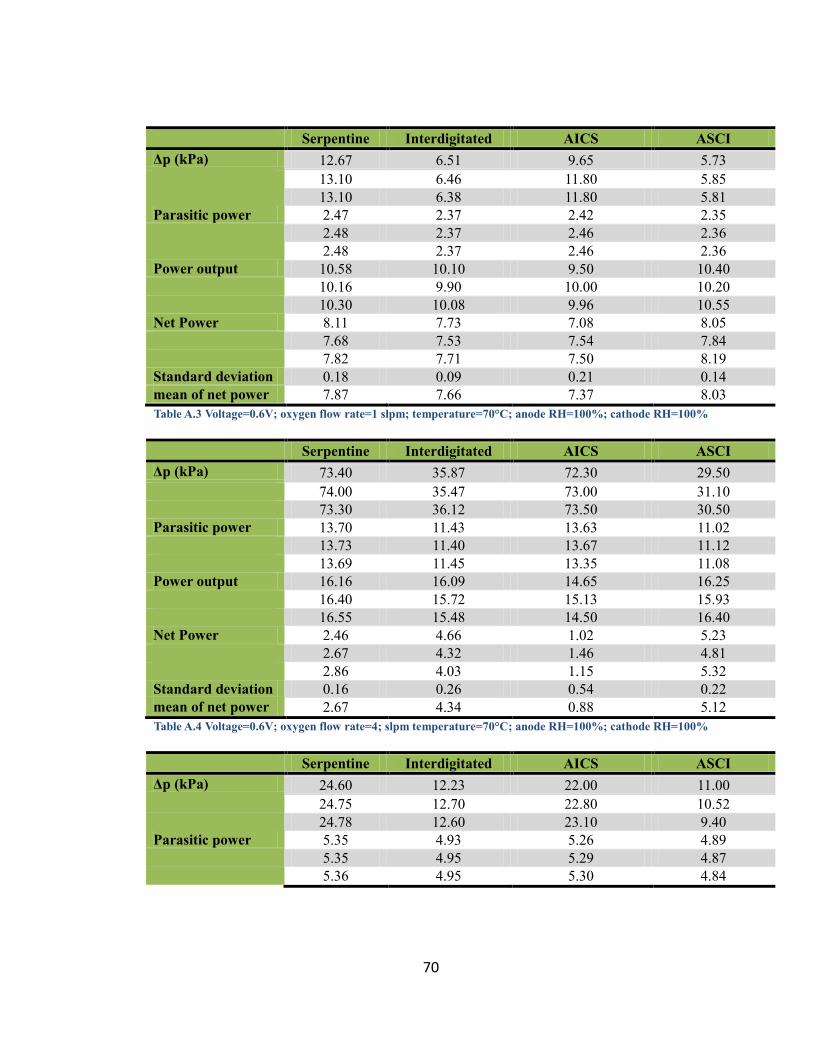
70
Serpentine Interdigitated AICS ASCI
Δp (kPa) 12.67 6.51 9.65 5.73
13.10 6.46 11.80 5.85
13.10 6.38 11.80 5.81
Parasitic power 2.47 2.37 2.42 2.35
2.48 2.37 2.46 2.36
2.48 2.37 2.46 2.36
Power output 10.58 10.10 9.50 10.40
10.16 9.90 10.00 10.20
10.30 10.08 9.96 10.55
Net Power 8.11 7.73 7.08 8.05
7.68 7.53 7.54 7.84
7.82 7.71 7.50 8.19
Standard deviation 0.18 0.09 0.21 0.14
mean of net power 7.87 7.66 7.37 8.03
Table A.3 Voltage=0.6V; oxygen flow rate=1 slpm; temperature=70°C; anode RH=100%; cathode RH=100%
Serpentine Interdigitated AICS ASCI
Δp (kPa) 73.40 35.87 72.30 29.50
74.00 35.47 73.00 31.10
73.30 36.12 73.50 30.50
Parasitic power 13.70 11.43 13.63 11.02
13.73 11.40 13.67 11.12
13.69 11.45 13.35 11.08
Power output 16.16 16.09 14.65 16.25
16.40 15.72 15.13 15.93
16.55 15.48 14.50 16.40
Net Power 2.46 4.66 1.02 5.23
2.67 4.32 1.46 4.81
2.86 4.03 1.15 5.32
Standard deviation 0.16 0.26 0.54 0.22
mean of net power 2.67 4.34 0.88 5.12
Table A.4 Voltage=0.6V; oxygen flow rate=4; slpm temperature=70°C; anode RH=100%; cathode RH=100%
Serpentine Interdigitated AICS ASCI
Δp (kPa) 24.60 12.23 22.00 11.00
24.75 12.70 22.80 10.52
24.78 12.60 23.10 9.40
Parasitic power 5.35 4.93 5.26 4.89
5.35 4.95 5.29 4.87
5.36 4.95 5.30 4.84
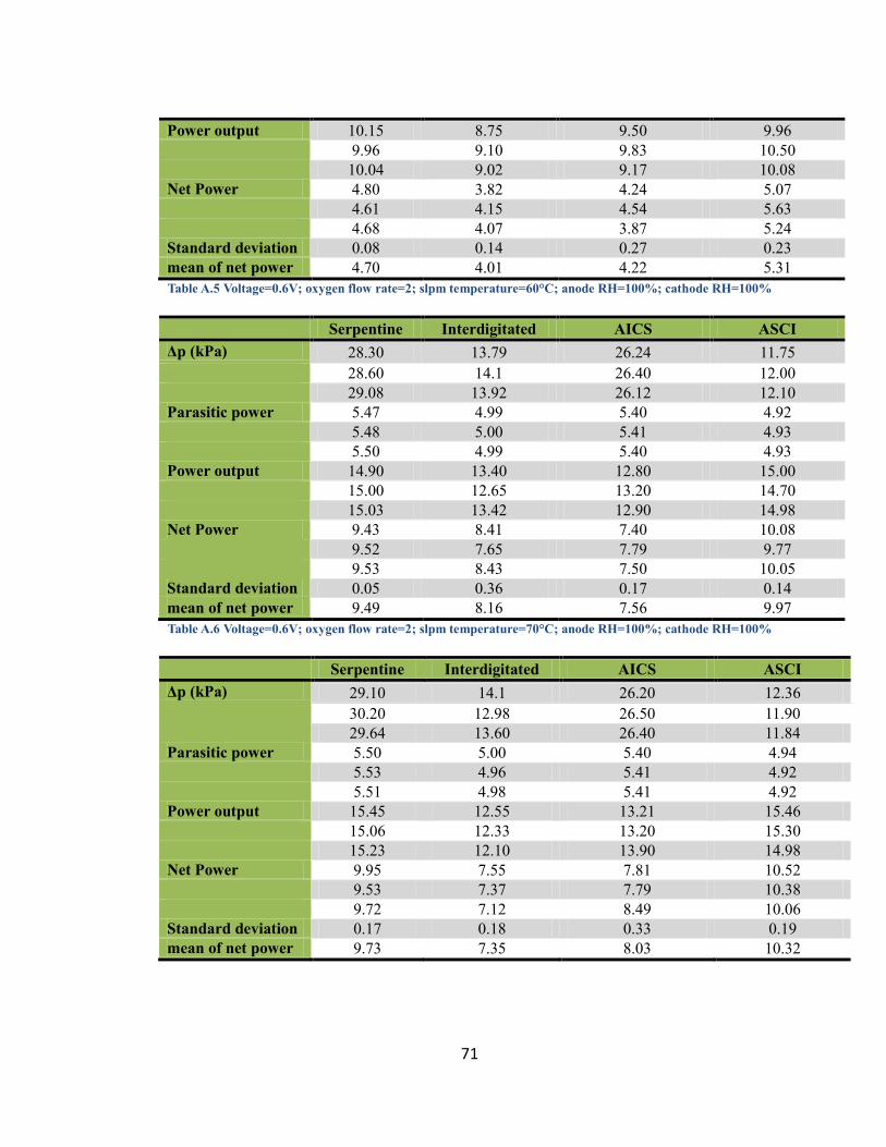
71
Power output 10.15 8.75 9.50 9.96
9.96 9.10 9.83 10.50
10.04 9.02 9.17 10.08
Net Power 4.80 3.82 4.24 5.07
4.61 4.15 4.54 5.63
4.68 4.07 3.87 5.24
Standard deviation 0.08 0.14 0.27 0.23
mean of net power 4.70 4.01 4.22 5.31
Table A.5 Voltage=0.6V; oxygen flow rate=2; slpm temperature=60°C; anode RH=100%; cathode RH=100%
Serpentine Interdigitated AICS ASCI
Δp (kPa) 28.30 13.79 26.24 11.75
28.60 14.1 26.40 12.00
29.08 13.92 26.12 12.10
Parasitic power 5.47 4.99 5.40 4.92
5.48 5.00 5.41 4.93
5.50 4.99 5.40 4.93
Power output 14.90 13.40 12.80 15.00
15.00 12.65 13.20 14.70
15.03 13.42 12.90 14.98
Net Power 9.43 8.41 7.40 10.08
9.52 7.65 7.79 9.77
9.53 8.43 7.50 10.05
Standard deviation 0.05 0.36 0.17 0.14
mean of net power 9.49 8.16 7.56 9.97
Table A.6 Voltage=0.6V; oxygen flow rate=2; slpm temperature=70°C; anode RH=100%; cathode RH=100%
Serpentine Interdigitated AICS ASCI
Δp (kPa) 29.10 14.1 26.20 12.36
30.20 12.98 26.50 11.90
29.64 13.60 26.40 11.84
Parasitic power 5.50 5.00 5.40 4.94
5.53 4.96 5.41 4.92
5.51 4.98 5.41 4.92
Power output 15.45 12.55 13.21 15.46
15.06 12.33 13.20 15.30
15.23 12.10 13.90 14.98
Net Power 9.95 7.55 7.81 10.52
9.53 7.37 7.79 10.38
9.72 7.12 8.49 10.06
Standard deviation 0.17 0.18 0.33 0.19
mean of net power 9.73 7.35 8.03 10.32
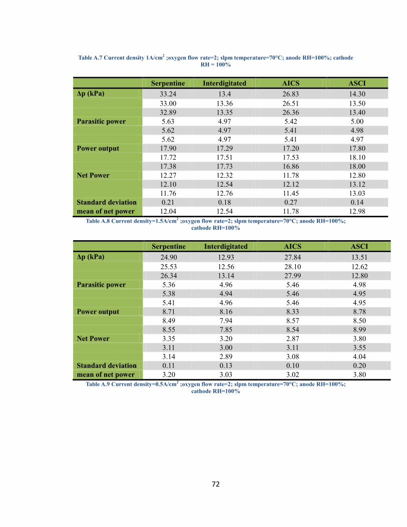
72
Table A.7 Current density 1A/cm2 ;oxygen flow rate=2; slpm temperature=70°C; anode RH=100%; cathode
RH = 100%
Serpentine Interdigitated AICS ASCI
Δp (kPa) 33.24 13.4 26.83 14.30
33.00 13.36 26.51 13.50
32.89 13.35 26.36 13.40
Parasitic power 5.63 4.97 5.42 5.00
5.62 4.97 5.41 4.98
5.62 4.97 5.41 4.97
Power output 17.90 17.29 17.20 17.80
17.72 17.51 17.53 18.10
17.38 17.73 16.86 18.00
Net Power 12.27 12.32 11.78 12.80
12.10 12.54 12.12 13.12
11.76 12.76 11.45 13.03
Standard deviation 0.21 0.18 0.27 0.14
mean of net power 12.04 12.54 11.78 12.98
Table A.8 Current density=1.5A/cm2 ;oxygen flow rate=2; slpm temperature=70°C; anode RH=100%;
cathode RH=100%
Serpentine Interdigitated AICS ASCI
Δp (kPa) 24.90 12.93 27.84 13.51
25.53 12.56 28.10 12.62
26.34 13.14 27.99 12.80
Parasitic power 5.36 4.96 5.46 4.98
5.38 4.94 5.46 4.95
5.41 4.96 5.46 4.95
Power output 8.71 8.16 8.33 8.78
8.49 7.94 8.57 8.50
8.55 7.85 8.54 8.99
Net Power 3.35 3.20 2.87 3.80
3.11 3.00 3.11 3.55
3.14 2.89 3.08 4.04
Standard deviation 0.11 0.13 0.10 0.20
mean of net power 3.20 3.03 3.02 3.80
Table A.9 Current density=0.5A/cm2 ;oxygen flow rate=2; slpm temperature=70°C; anode RH=100%;
cathode RH=100%
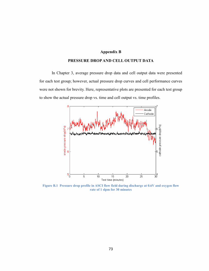
73
Appendix B
PRESSURE DROP AND CELL OUTPUT DATA
In Chapter 3, average pressure drop data and cell output data were presented
for each test group; however, actual pressure drop curves and cell performance curves
were not shown for brevity. Here, representative plots are presented for each test group
to show the actual pressure drop vs. time and cell output vs. time profiles.
Figure B.1 Pressure drop profile in ASCI flow field during discharge at 0.6V and oxygen flow
rate of 1 slpm for 30 minutes
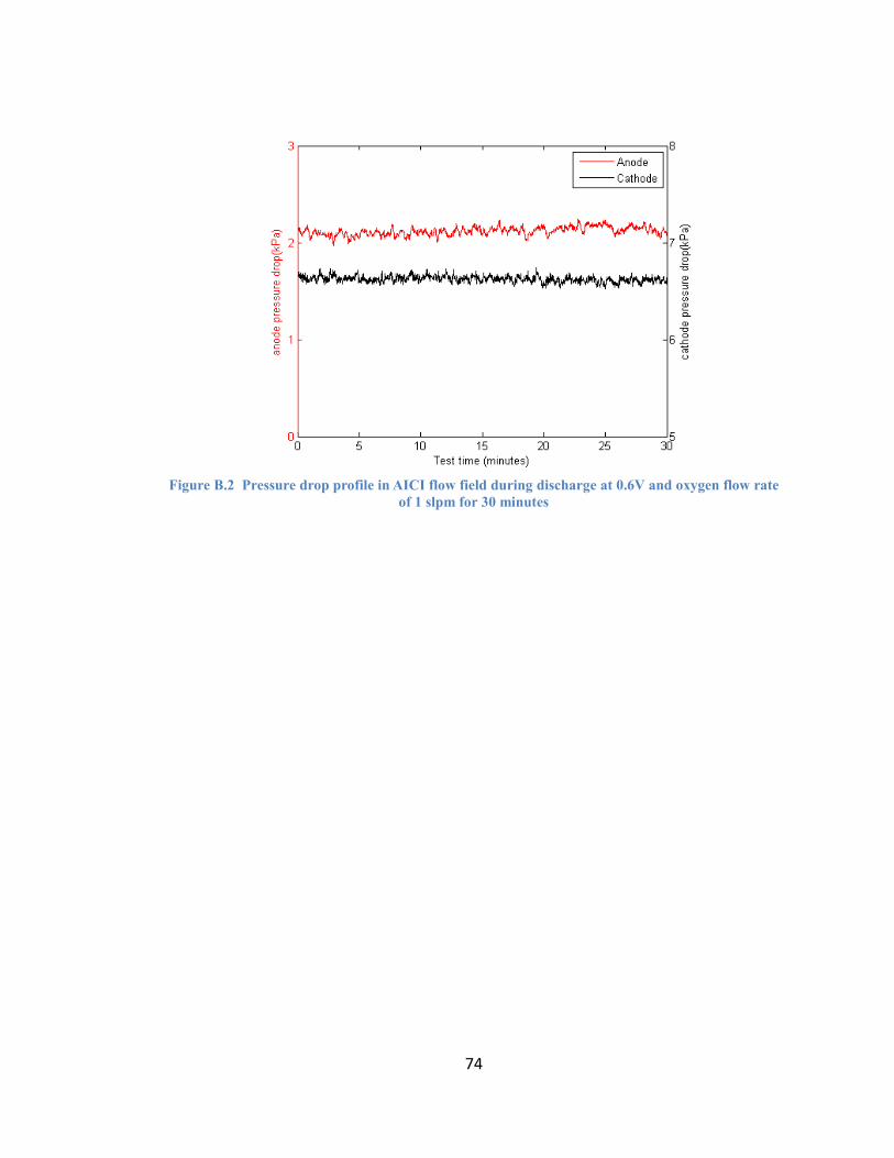
74
Figure B.2 Pressure drop profile in AICI flow field during discharge at 0.6V and oxygen flow rate
of 1 slpm for 30 minutes

75
Figure B.3 Pressure drop profile in ASCS flow field during discharge at 0.6V and oxygen flow
rate of 1 slpm for 30 minutes
Figure B.4 Pressure drop profile in ASCI flow field during discharge at 0.6V and oxygen flow
rate of 4 slpm for 30 minutes

76
Figure B.5 Pressure drop profile in AICI flow field during discharge at 0.6V and oxygen flow
rate of 4 slpm for 30 minutes
Figure B.6 Pressure drop profile in ASCS flow field during discharge at 0.6V and oxygen flow
rate of 4 slpm for 30 minutes

77
Figure B.7 Pressure drop profile in ASCI flow field during discharge at 0.6V cathode RH 50%
for 30 minutes
Figure B.8 Pressure drop profile in AICI flow field during discharge at 0.6V and cathode RH
50% for 30 minutes
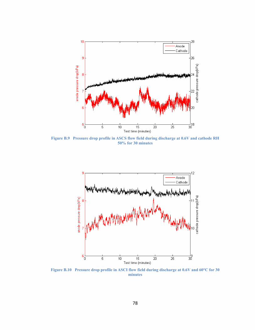
78
Figure B.9 Pressure drop profile in ASCS flow field during discharge at 0.6V and cathode RH
50% for 30 minutes
Figure B.10 Pressure drop profile in ASCI flow field during discharge at 0.6V and 60°C for 30
minutes

79
Figure B.11 Pressure drop profile in AICS flow field during discharge at 0.6V and 60°C for 30
minutes
Figure B.12 Pressure drop profile in AICI flow field during discharge at 0.6V and 60°C for 30
minute

80
Figure B.13 Pressure drop profile in ASCI flow field during discharge at 0.6V and 60°C for 30
minutes
Figure B.14 Performance profile in AICI flow field during discharge at 0.6V under standard
operating condition for 30 minutes
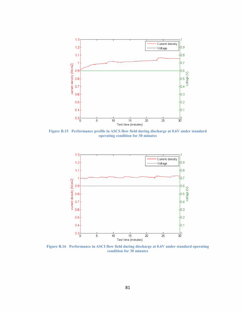
81
Figure B.15 Performance profile in ASCS flow field during discharge at 0.6V under standard
operating condition for 30 minutes
Figure B.16 Performance in ASCI flow field during discharge at 0.6V under standard operating
condition for 30 minutes

82
Figure B.17 Performance profile in AICS flow field during discharge at 0.6V under standard
operating condition for 30 minutes
Figure B.18 Performance profile in AICS flow field during discharge at 0.6V and 60°C for 30
minutes

83
Figure B.19 Performance profile in ASCS flow field during discharge at 0.6V and 60°C for 30
minutes
Figure B.20 Performance profile in AICI flow field during discharge at 0.6V and 60°C for 30
minutes

84
Figure B.21 Performance profile in AICS flow field during discharge at 0.6V and cathode RH
50% for 30 minutes
Figure B.22 Performance profile in AICI flow field during discharge at 0.6V cathode RH 50%
for 30 minutes

85
Figure B.23 Performance profile in ASCS flow field during discharge at 0.6V and cathode RH
50% for 30 minutes
Figure B.24 Performance profile in AICS flow field during discharge at 0.6V and oxygen flow
rate of 4 slpm for 30 minutes

86
Figure B.25 Performance profile in AICI flow field during discharge at 0.6V and oxygen flow
rate of 4 slpm for 30 minutes
Figure B.26 Performance profile in ASCS flow field during discharge at 0.6V and oxygen flow
rate of 4 slpm for 30 minutes

87
Figure B.27 Performance profile in ASCS flow field during discharge at 0.5A/cm
2 for 30 minutes
Figure B.28 Performance profile in AICS flow field during discharge at 0.5A/cm
2 for 30 minutes
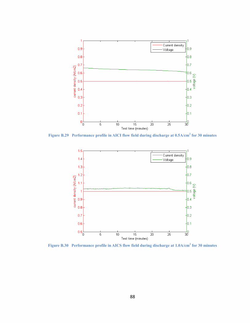
88
Figure B.29 Performance profile in AICI flow field during discharge at 0.5A/cm
2 for 30 minutes
Figure B.30 Performance profile in AICS flow field during discharge at 1.0A/cm
2 for 30 minutes

89
Figure B.31 Performance profile in AICI flow field during discharge at 1.0A/cm
2 for 30 minutes
Figure B.32 Performance profile ASCS flow field during discharge at 1.0A/cm
2 for 30 minutes
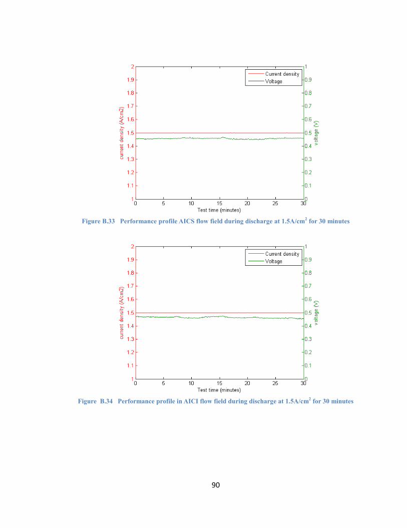
90
Figure B.33 Performance profile AICS flow field during discharge at 1.5A/cm
2 for 30 minutes
Figure B.34 Performance profile in AICI flow field during discharge at 1.5A/cm
2 for 30 minutes

91
Figure B.35 Performance profile in ASCS flow field during discharge at 1.5A/cm
2 for 30 minutes

92
Appendix C
PERMISSION FOR FIGURE USAGE
Figure 1.1 and Fig. 1.2 in Chapter 1 were created by other researchers and used
in their previous publications. To use those figures in this thesis, we got the permission
from the authors and publisher.
Permission for using Fig. 1.1:
Fang Ruan <[email protected]>
permission for using one figure in your paper
3 messages
Fang Ruan <[email protected]> Wed, Jan 8, 2014 at 4:54
PM To: Glenn Catlin <[email protected]>
Hi Glenn, I'm writing my master thesis now, and in the introduction part I used a figure in your thesis and I put your thesis in the reference list. Can you give me the permission for using this figure? Thanks a lot! Best, -- Fang
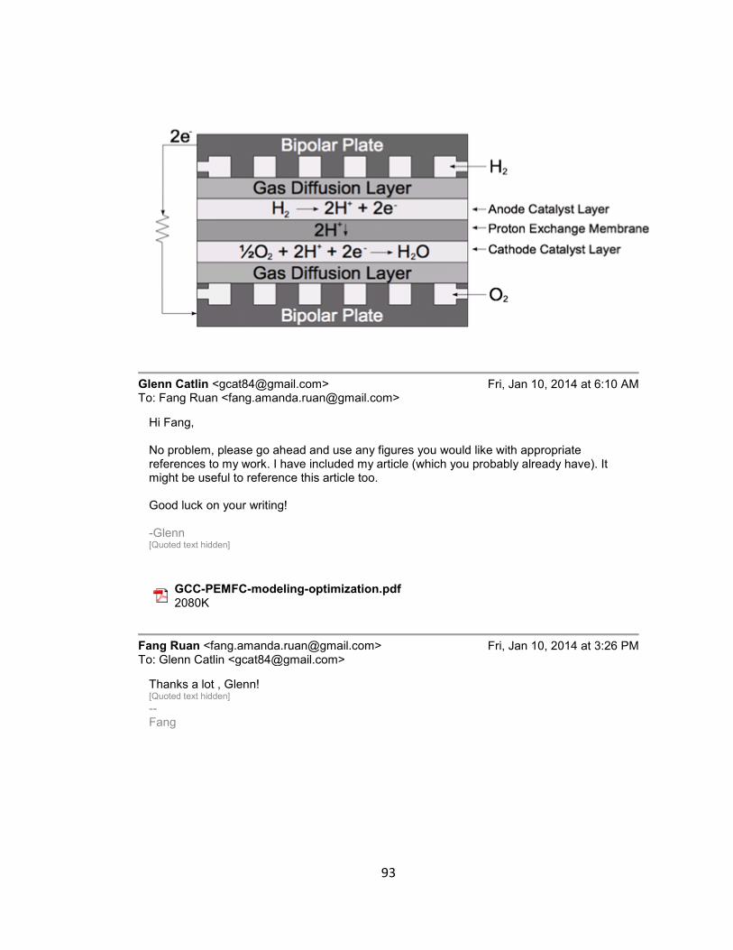
93
Glenn Catlin <[email protected]> Fri, Jan 10, 2014 at 6:10 AM To: Fang Ruan <[email protected]>
Hi Fang, No problem, please go ahead and use any figures you would like with appropriate references to my work. I have included my article (which you probably already have). It might be useful to reference this article too. Good luck on your writing! -Glenn [Quoted text hidden]
GCC-PEMFC-modeling-optimization.pdf 2080K
Fang Ruan <[email protected]> Fri, Jan 10, 2014 at 3:26 PM To: Glenn Catlin <[email protected]>
Thanks a lot , Glenn! [Quoted text hidden] -- Fang

94
Permission for using Fig. 1.2:
ELSEVIER LICENSE TERMS AND CONDITIONS Jan 27, 2014
This is a License Agreement between FANG RUAN ("You") and Elsevier
("Elsevier") provided by
Copyright Clearance Center ("CCC"). The license consists of your order details,
the terms and
conditions provided by Elsevier, and the payment terms and conditions. All payments must be made in full to CCC. For payment instructions, please see
information listed at the bottom of this form.
Supplier Elsevier Limited
The Boulevard,Langford Lane
Kidlington,Oxford,OX5 1GB,UK
Registered Company
Number
1982084
Customer name FANG RUAN
Customer address 1063 MORSE AVE
SUNNYVALE, CA 94089
License number 3317391148387
License date Jan 27, 2014
Licensed content publisher Elsevier
Licensed content
publication
Journal of Power Sources
Licensed content title Performance studies of PEM fuel cells with interdigitated flow
fields
Licensed content author Lin Wang,Hongtan Liu
Licensed content date 12 August 2004
Licensed content volume
number
134
Licensed content issue
number
2
Number of pages 12
Start Page 185
End Page 196
Type of Use reuse in a thesis/dissertation
Portion figures/tables/illustrations
Number of
figures/tables/illustrations
1
Format both print and electronic
Are you the author of this

95
Elsevier article?
No 1/27/14 Rightslink Printable License https://s100.copyright.com/AppDispatchServlet 2/7
Will you be translating? No
Title of your
thesis/dissertation
Net power output and pressure drop behavior of PEM fuel cells
with serpentine and interdigitated flow fields
Expected completion date Feb 2014
Estimated size (number of
pages)
106
Elsevier VAT number GB 494 6272 12
Permissions price 0.00 USD
VAT/Local Sales Tax 0.00 USD / 0.00 GBP
Total 0.00 USD
Terms and Conditions
INTRODUCTION
1. The publisher for this copyrighted material is Elsevier. Byclicking "accept"
in connection with
completing this licensingtransaction, you agree that the following terms and
conditions apply to
thistransaction (along with the Billing and Payment terms and
conditionsestablished by Copyright
Clearance Center, Inc. ("CCC"), at the timethat you opened your Rightslink
account and that are
available at any time at http://myaccount.copyright.com).
GENERAL TERMS
2. Elsevier hereby grants you permission to reproduce the
aforementionedmaterial subject to the
terms and conditions indicated.
3. Acknowledgement: If any part of the material to be used (for
example,figures) has appeared in
our publication with credit or acknowledgement toanother source, permission
must also be sought
from that source. If suchpermission is not obtained then that material may not
be included in
yourpublication/copies. Suitable acknowledgement to the source must be made,
eitheras a footnote
or in a reference list at the end of your publication, asfollows:
“Reprinted from Publication title, Vol /edition number, Author(s), Title
ofarticle / title of chapter,

96
Pages No., Copyright (Year), with permission fromElsevier [OR
APPLICABLE SOCIETY
COPYRIGHT OWNER].” Also Lancet special credit -“Reprinted from The
Lancet, Vol. number,
Author(s), Title of article, PagesNo., Copyright (Year), with permission from
Elsevier.”
4. Reproduction of this material is confined to the purpose and/or media
forwhich permission is
hereby given.
5. Altering/Modifying Material: Not Permitted. However figures
andillustrations may be
altered/adapted minimally to serve your work. Any otherabbreviations,
additions, deletions and/or
any other alterations shall be madeonly with prior written authorization of
Elsevier Ltd. (Please
contact Elsevierat [email protected])
6. If the permission fee for the requested use of our material is waived inthis
instance, please be
advised that your future requests for Elseviermaterials may attract a fee. 1/27/14 Rightslink Printable License https://s100.copyright.com/AppDispatchServlet 3/7
7. Reservation of Rights: Publisher reserves all rights not specificallygranted in
the combination of (i)
the license details provided by you andaccepted in the course of this licensing
transaction, (ii) these
terms andconditions and (iii) CCC's Billing and Payment terms and conditions.
8. License Contingent Upon Payment: While you may exercise the
rightslicensed immediately upon
issuance of the license at the end of the licensingprocess for the transaction,
provided that you have
disclosed complete andaccurate details of your proposed use, no license is
finally effective
unlessand until full payment is received from you (either by publisher or by
CCC) asprovided in
CCC's Billing and Payment terms and conditions. If fullpayment is not received
on a timely basis,
then any license preliminarilygranted shall be deemed automatically revoked
and shall be void as if
nevergranted. Further, in the event that you breach any of these terms
andconditions or any of

97
CCC's Billing and Payment terms and conditions, thelicense is automatically
revoked and shall be
void as if never granted. Use of materials as described in a revoked license, as
well as any use of
thematerials beyond the scope of an unrevoked license, may constitute
copyrightinfringement and
publisher reserves the right to take any and all action toprotect its copyright in
the materials.
9. Warranties: Publisher makes no representations or warranties with respectto
the licensed
material.
10. Indemnity: You hereby indemnify and agree to hold harmless publisher
andCCC, and their
respective officers, directors, employees and agents, from andagainst any and
all claims arising out
of your use of the licensed materialother than as specifically authorized
pursuant to this license.
11. No Transfer of License: This license is personal to you and may not
besublicensed, assigned, or
transferred by you to any other person withoutpublisher's written permission.
12. No Amendment Except in Writing: This license may not be amended
exceptin a writing signed
by both parties (or, in the case of publisher, by CCC onpublisher's behalf).
13. Objection to Contrary Terms: Publisher hereby objects to any
termscontained in any purchase
order, acknowledgment, check endorsement or otherwriting prepared by you,
which terms are
inconsistent with these terms andconditions or CCC's Billing and Payment
terms and conditions.
These termsand conditions, together with CCC's Billing and Payment terms and
conditions(which
are incorporated herein), comprise the entire agreement between you
andpublisher (and CCC)
concerning this licensing transaction. In the eventof any conflict between your
obligations
established by these terms andconditions and those established by CCC's
Billing and Payment
terms andconditions, these terms and conditions shall control.
14. Revocation: Elsevier or Copyright Clearance Center may deny
thepermissions described in this

98
License at their sole discretion, for any reasonor no reason, with a full refund
payable to you.
Notice of such denialwill be made using the contact information provided by
you. Failure toreceive
such notice will not alter or invalidate the denial. In no eventwill Elsevier or
Copyright Clearance
Center be responsible or liable for anycosts, expenses or damage incurred by
you as a result of a
denial of yourpermission request, other than a refund of the amount(s) paid by
you toElsevier
and/or Copyright Clearance Center for denied permissions.
LIMITED LICENSE 1/27/14 Rightslink Printable License https://s100.copyright.com/AppDispatchServlet 4/7
The following terms and conditions apply only to specific license types:
15. Translation: This permission is granted fornon-exclusive world English
rights only unless
yourlicense was granted for translation rights. If you licensed translation
rightsyou may only translate
this content into the languages you requested. Aprofessional translator must
perform all translations
and reproduce the contentword for word preserving the integrity of the article.
If this license is toreuse
1 or 2 figures then permission is granted for non-exclusive world rightsin all
languages.
16. Posting licensed content on any Website: The followingterms and
conditions apply as
follows: Licensing material from an Elsevierjournal: All content posted to the
web site must maintain
the copyright informationline on the bottom of each image; A hyper-text must
be included to the
Homepageof the journal from which you are licensing at
http://www.sciencedirect.com/science/journal/xxxxx orthe Elsevier homepage
for books at
http://www.elsevier.com; CentralStorage: This license does not include
permission for a scanned
version of thematerial to be stored in a central repository such as that provided
byHeron/XanEdu.
Licensing material from an Elsevier book: A hyper-text link must be includedto
the Elsevier

99
homepage at http://www.elsevier.com . Allcontent posted to the web site must
maintain the
copyright information line onthe bottom of each image.
Posting licensed content on Electronic reserve: In addition to the above the
following
clausesare applicable: The web site must be password-protected and made
available onlyto bona
fide students registered on a relevant course. This permission isgranted for 1
year only. You may
obtain a new license for future websiteposting.
For journal authors: the following clauses are applicable inaddition to the
above: Permission
granted is limited to the author acceptedmanuscript version* of your paper.
*Accepted Author Manuscript (AAM) Definition: An accepted
authormanuscript (AAM) is
the author’s version of the manuscript of an article thathas been accepted for
publication and which
may include any author-incorporatedchanges suggested through the processes
of submission
processing, peer review,and editor-author communications. AAMs do not
include other
publishervalue-added contributions such as copy-editing, formatting,
technicalenhancements and (if
relevant) pagination.
You are not allowed to download and post the published journal article
(whetherPDF or HTML,
proof or final version), nor may you scan the printed edition tocreate an
electronic version. A
hyper-text must be included to the Homepage ofthe journal from which you are
licensing at
http://www.sciencedirect.com/science/journal/xxxxx. As part of our normal
production process,
you will receive an e-mail noticewhen your article appears on Elsevier’s online
service
ScienceDirect(www.sciencedirect.com). That e-mail will include the article’s
Digital
ObjectIdentifier (DOI). This number provides the electronic link to the
publishedarticle and should
be included in the posting of your personal version. We askthat you wait until
you receive this email

100
and have the DOI to do any posting.
Posting to a repository: Authorsmay post their AAM immediately to their
employer’s institutional
repository forinternal use only and may make their manuscript publically
available after thejournal1/
27/14 Rightslink Printable License https://s100.copyright.com/AppDispatchServlet 5/7
specific embargo period has ended.
Please also refer to Elsevier'sArticle Posting Policy for further information.
18. For book authors the following clauses are applicable in addition tothe
above: Authors are
permitted to place a briefsummary of their work online only.. You are
notallowed to download and
post the published electronic version of your chapter,nor may you scan the
printed edition to create
an electronic version. Posting to a repository: Authors arepermitted to post a
summary of their
chapter only in their institution’srepository.
20. Thesis/Dissertation: If your license is for use in athesis/dissertation your
thesis may be
submitted to your institution in eitherprint or electronic form. Should your
thesis be published
commercially, pleasereapply for permission. These requirements include
permission for the
Libraryand Archives of Canada to supply single copies, on demand, of the
completethesis and
include permission for UMI to supply single copies, on demand, ofthe complete
thesis. Should your
thesis be published commercially, pleasereapply for permission.
Elsevier Open Access Terms andConditions
Elsevier publishes Open Access articles in both its Open Access journals andvia
its Open Access
articles option in subscription journals.
Authors publishing in an Open Access journal or who choose to make
theirarticle Open Access in
an Elsevier subscription journal select one of thefollowing Creative Commons
user licenses, which
define how a reader may reusetheir work: Creative Commons Attribution
License (CC BY),

101
Creative CommonsAttribution – Non Commercial - ShareAlike (CC BY
NCSA) and Creative
Commons Attribution – Non Commercial – No Derivatives (CC BYNC ND)
Terms & Conditions applicable toall Elsevier Open Access articles:
Any reuse of the article must not represent the author as endorsing
theadaptation of the article nor
should the article be modified in such a way asto damage the author’s honour or
reputation.
The author(s) must be appropriately credited.
If any part of the material to be used (for example, figures) has appearedin our
publication with
credit or acknowledgement to another source it is theresponsibility of the user
to ensure their reuse
complies with the terms andconditions determined by the rights holder.
Additional Terms & Conditionsapplicable to each Creative Commons user
license:
CC BY: You may distribute andcopy the article, create extracts, abstracts, and
other revised
versions,adaptations or derivative works of or from an article (such as a
translation),to include in a
collective work (such as an anthology), to text or data minethe article, including
for commercial
purposes without permission from Elsevier 1/27/14 Rightslink Printable License https://s100.copyright.com/AppDispatchServlet 6/7
CC BY NC SA: For non-commercialpurposes you may distribute and copy the
article, create
extracts, abstractsand other revised versions, adaptations or derivative works of
or from anarticle
(such as a translation), to include in a collective work (such as ananthology), to
text and data mine
the article and license new adaptations or creationsunder identical terms without
permission from
Elsevier
CC BY NC ND: For non-commercialpurposes you may distribute and copy the
article and
include it in a collectivework (such as an anthology), provided you do not alter
or modify the
article,without permission from Elsevier
Any commercial reuse of Open Access articles published with a CC BY NC SA

102
or CC BY NC NDlicense requires permission from Elsevier and will be subject
to a
fee.
Commercial reuse includes:
· Promotional purposes (advertising or marketing)
· Commercial exploitation ( e.g. a product forsale or loan)
· Systematic distribution (for a fee or free ofcharge)
Please refer to Elsevier'sOpen Access Policy for further information.
21. Other Conditions:
v1.7 If you would like to pay for this license now, please remit this license along with your
payment made payable to "COPYRIGHT CLEARANCE CENTER" otherwise you will be
invoiced within 48 hours of the license date. Payment should be in the form of a check or
money order referencing your account number and this invoice number RLNK501212311.
Once you receive your invoice for this order, you may pay your invoice by credit card.
Please follow instructions provided at that time.
Make Payment To:
Copyright Clearance Center
Dept 001
P.O. Box 843006
Boston, MA 02284-3006
For suggestions or comments regarding this order, contact RightsLink Customer Support:
[email protected] or +1-877-622-5543 (toll free in the US) or +1-978-646-
2777.
Gratis licenses (referencing $0 in the Total field) are free. Please retain this printable
license for your reference. No payment is required.