Design of an Algae Harvesting Cable Robot, Including a Novel Solution to the Forward

Pose Kinematics Problem

A thesis presented to

the faculty of

the Russ College of Engineering and Technology of Ohio University

In partial fulfillment

of the requirements for the degree

Master of Science

Noah J. Needler

August 2013

© 2013 Noah J. Needler. All Rights Reserved.

2

This thesis titled

Design of an Algae Harvesting Cable Robot, Including a Novel Solution to the Forward

Pose Kinematics Problem

by

NOAH J. NEEDLER

has been approved for

the Department of Mechanical Engineering

and the Russ College of Engineering and Technology by

Robert L. Williams II

Professor of Mechanical Engineering

Dennis Irwin

Dean, Russ College of Engineering and Technology

3

Abstract

NEEDLER, NOAH J., M.S., August 2013, Mechanical Engineering

Design of an Algae Harvesting Cable Robot, Including a Novel Solution to the Forward

Pose Kinematics Problem

Director of Thesis: Robert L. Williams II

A cable robot system is proposed for implementation as an algae harvesting tool.

The proposed system consists of four cables that run from four winches, up and over four

adjustable towers, and meet at a point on t he robot’s end-effector. The robot is to be

controlled by a PID controller that controls all cables independently, but simultaneously.

The research consists of robot kinematics/dynamics analyses, MATLAB simulation, and

design.

In addition to providing a simplified method of solving the forward pose

kinematics problem, this research shows that to minimize cable tension, the towers

should be at least 1.5 times the maximum height of the end effector, which can be set by

the operator. This result is verified by a simulation in which the tower heights are varied,

showing a rapid decrease in tension as tower height increases. In addition, cable

parameters are determined and four possible end effectors designs are proposed.

4

Dedication

This work is dedicated to Dr. Bob, world-class teacher and advisor.

5

Acknowledgments

The author would like to acknowledge the following for their support on this

project:

Dr. Robert Williams, without his instruction and guidance this research would not

have been possible, Dr. Hajrudin Pasic, whose constant encouragement was an

inspiration, committee members Dr. David Bayless and Dr. Morgan Vis-Chiasson, whose

feedback and flexibility were invaluable, Jesus Pagan, who provided valuable experience

and information, and Dr. Sara Wiseman, for her patience, support, and love.

6

Table of Contents

Page

Abstract ............................................................................................................................... 3 Dedication ........................................................................................................................... 4 Acknowledgments............................................................................................................... 5 List of Figures ..................................................................................................................... 8 List of Tables .................................................................................................................... 10 1. Background ............................................................................................................... 11

1.1 Algae ................................................................................................................. 14 1.1.1 Cultivation..................................................................................................... 14 1.1.2 Harvest .......................................................................................................... 15 1.1.3 Dewatering .................................................................................................... 16 1.1.4 Extraction ...................................................................................................... 17 1.1.5 Other Uses ..................................................................................................... 19 1.1.6 Current Interest ............................................................................................. 21

1.2 Cable Robots ..................................................................................................... 22 1.2.1 Applications .................................................................................................. 22 1.2.2 Under-constrained vs. Fully-constrained ...................................................... 22 1.2.3 Method of Control......................................................................................... 23 1.2.4 Current Interest ............................................................................................. 25 1.2.5 Proposed Cable Robot Design ...................................................................... 25

2. Thesis Objectives ...................................................................................................... 29 3. Analysis ..................................................................................................................... 30

3.1 Definitions......................................................................................................... 30 3.2 Workspace......................................................................................................... 32 3.3 Kinematics ........................................................................................................ 32

3.3.1 Inverse Pose Kinematics Analysis ................................................................ 32 3.3.2 Novel Forward Pose Kinematics Analysis ................................................... 33 3.3.3 Velocity Kinematics Analysis ....................................................................... 38 3.3.4 Resolved-Rate Control Solution ................................................................... 41 3.3.5 Acceleration Kinematics Analysis ................................................................ 41 3.3.6 Cable/Cable Reel Kinematics ....................................................................... 42

3.4 Pseudostatics ..................................................................................................... 43 3.4.1 Static Equilibrium ......................................................................................... 43 3.4.2 Forward Pseudostatics Solution .................................................................... 45 3.4.3 Inverse Pseudostatics Solution ...................................................................... 45 3.4.4 Singularities .................................................................................................. 46 3.4.5 Cable Tension/Actuator Torque .................................................................... 46 3.4.6 Translational Stiffness .................................................................................. 47

3.5 Dynamics .......................................................................................................... 48 3.5.1 Dynamics Equations of Motion .................................................................... 49 3.5.2 Inverse Dynamics Solution ........................................................................... 50

7

3.5.3 Forward Dynamics Solution ......................................................................... 51 3.5.4 Actuator/Cable Reel Dynamics ..................................................................... 52

3.6 PID Controller Design ...................................................................................... 56 3.6.1 Potential Errors and Disturbances ................................................................. 62 3.6.2 Design Example ............................................................................................ 62

4. Simulation & Design Decisions ................................................................................ 65 4.1 Snapshot Examples ........................................................................................... 66 4.2 Single Point Harvest ......................................................................................... 67 4.3 Corner to Corner Harvest .................................................................................. 71 4.4 Tower Choice .................................................................................................... 75 4.5 Appropriate Tower Height ................................................................................ 76 4.6 Cable Choice ..................................................................................................... 92

4.6.1 Examples ....................................................................................................... 93 4.7 End Effector Design .......................................................................................... 97

4.7.1 Design 1: Mesh Filter.................................................................................... 98 4.7.2 Design 2: Rotating net .................................................................................. 99 4.7.3 Design 3: Cage ............................................................................................ 101 4.7.4 Design 4: Stationary Cage .......................................................................... 102 4.7.5 Design 5: Stationary Mesh Filter ................................................................ 103

4.8 Robot Control.................................................................................................. 105 5. Conclusions and Recommendation ......................................................................... 106

5.1 Conclusions ..................................................................................................... 106 5.2 Recommendations ........................................................................................... 108

Works Cited .................................................................................................................... 110 Appendix: ........................................................................................................................ 114

MATLAB Code .......................................................................................................... 114 Algae.m ................................................................................................................... 114 algaeplot.m .............................................................................................................. 116 algaepose.m ............................................................................................................. 118 algaesurft.m ............................................................................................................. 120 algfigs.m .................................................................................................................. 122 corntocorn.m ........................................................................................................... 124 define.m .................................................................................................................. 126 justraise.m ............................................................................................................... 128 oneharvest.m ........................................................................................................... 130 snaps.m .................................................................................................................... 134 towervary.m ............................................................................................................ 136

8

List of Figures

Page Figure 1: Import dependency for the U.S. [1] ................................................................... 11 Figure 2: Lipid Extraction from algae biomass [13] ......................................................... 18 Figure 3: Processing for algae biomass [16] ..................................................................... 19 Figure 4: Reclaiming fossil fuel emissions for use in biofuel production [22] ................ 21 Figure 5: Feedback control loop block diagram [33]........................................................ 23 Figure 6: Solid Edge model of the proposed algae harvesting cable robot ...................... 26 Figure 7: Raceway pond [38] ............................................................................................ 27 Figure 8: Earthrise farm pond cluster [39] ........................................................................ 28 Figure 9: Algae harvesting robot diagram, including nomenclature ................................ 30 Figure 10: Diagram of the three-spheres approach ........................................................... 33 Figure 11: Free-body diagram of cable robot end effector. .............................................. 43 Figure 12: Cable tension/actuator statics free-body diagram ........................................... 47 Figure 13: Dynamics free-body diagram .......................................................................... 49 Figure 14: Single actuator/cable reel diagram .................................................................. 52 Figure 15: Actuator/cable reel free-body diagram ............................................................ 54 Figure 16: Single input, single output, negative feedback closed loop block diagram .... 57 Figure 17: MATLAB simulation of the proposed system ................................................ 65 Figure 18: Center point snapshot simulation .................................................................... 66 Figure 19: Snapshot example at [40 -30 4] ....................................................................... 67 Figure 20: End effector at the staging area for a 1 acre pond ........................................... 68 Figure 21: End effector at a harvest location of [60 40 0] ................................................ 68 Figure 22: Cable lengths as a function of time steps for a single harvest ......................... 69 Figure 23: End effector position as a function of time steps for a single harvest ............. 69 Figure 24: Cable velocities as a function of time steps for a single harvest ..................... 70 Figure 25: Cable tensions as a function of time steps for a single harvest ....................... 70 Figure 26: Stiffness norm as a function of time steps for a single harvest ....................... 71 Figure 27: End effector at the start of a corner-to-corner trajectory ................................. 71 Figure 28: End effector at the end of a corner-to-corner trajectory .................................. 72 Figure 29: Cable lengths as a function of time steps for a corner-to-corner trajectory .... 72 Figure 30: End effector position as a function of time for a corner-to-corner trajectory . 73 Figure 31: Cable velocities as a function of time for a corner-to-corner trajectory ......... 73 Figure 32: Cable tensions as a function of time for a corner-to-corner trajectory ............ 74 Figure 33: Stiffness norm as a function of time for a corner-to-corner trajectory ............ 74 Figure 34: Scorpion® tower from Alumina Tower Company, Inc. [43] .......................... 76 Figure 35: Standard pond setup with a center point harvest and 10 ft towers .................. 77 Figure 36: 1 acre pond, center harvest, 100 lbm, 10 ft towers, and vertical lift ............... 78 Figure 37: Standard pond setup with a center point harvest and 20 ft towers .................. 79 Figure 38: 1 acre pond, center harvest, 100 lbm, 20 ft towers, and vertical lift ............... 79 Figure 39: Standard pond setup with a center point harvest and 30 ft towers .................. 80 Figure 40: 1 acre pond, center harvest, 100 lbm, 30 ft towers, and vertical lift ............... 81

9 Figure 41: Standard pond setup with a [60 40] harvest and 10 ft towers ......................... 82 Figure 42: 1 acre pond, [60, 40] harvest, 100 lbm, 10 ft towers, and vertical lift ............ 82 Figure 43: Standard pond setup with a [-130 -80] harvest and 10 ft towers ..................... 83 Figure 44: 1 acre pond, [-130, -80] harvest, 100 lbm, 10 ft towers, and vertical lift ........ 84 Figure 45: 100’x100’ pond with a center harvest and 10 ft towers .................................. 85 Figure 46: 100’x100’ pond, center harvest, 100 lbm, 10 ft towers, and vertical lift ........ 85 Figure 47: 1 acre pond, center harvest, 50 lbm, 10 ft towers, and vertical lift ................. 86 Figure 48: 1 acre pond, center harvest, 200 lbm, 10 ft towers, and vertical lift ............... 87 Figure 49: 1 acre pond, center harvest, 100 lbm, and varying tower height ..................... 88 Figure 50: 1 acre pond, center harvest, 50 lbm, and varying tower height ....................... 89 Figure 51: ½ acre pond, center harvest, 100 lbm, and varying tower height .................... 90 Figure 52: 100’x100’ pond, center harvest, 100 lbm, and varying tower height .............. 90 Figure 53: 10’x10’ pond, center harvest, 100 lbm, and varying tower height .................. 91 Figure 54: Color plot of all four cables ............................................................................. 93 Figure 55: Color plot of T1 for a 1 acre pond, 100 lbm load, with 10 ft towers .............. 95 Figure 56: Color plot of T1 for a 1 acre pond, 50 lbm load, with 10 ft towers ................ 96 Figure 57: Color plot of T1 for a ½ acre pond, 100 lbm load, with 20 ft towers ............. 97 Figure 58: Solid Edge model of end effector design 1 ..................................................... 98 Figure 59: Solid Edge model of end effector design 2 ................................................... 100 Figure 60: Solid Edge model of end effector design 3 ................................................... 101 Figure 61: Solid Edge model of end effector design 4 ................................................... 103 Figure 62: Solid Edge model of end effector design 5 ................................................... 104

10

List of Tables

Page Table 1: Land area needed to replace transportation fuel consumption [6] ...................... 13 Table 2: Spectec-12 specifications [44] ............................................................................ 94

11

1. Background

Due to the increased costs and limited availability of fossil fuels, in addition to

environmental concerns, the race to obtain economically viable renewable energy sources

has become a global issue. Since the 1950’s, energy consumption in the United States has

increased dramatically, and the need for foreign importation has risen to meet the

demand.

Figure 1: Import dependency for the U.S. [1]

For years, researchers have been experimenting with various sources of energy

that can be produced locally. Many possible alternatives exist, each having both positive

and negative aspects; some examples include nuclear, wind, solar, and hydroelectric

energies.

12

Although nuclear energy has the potential for large scale power supply and is

currently being used throughout the world, there are growing concerns about its safety.

Nuclear accidents like Chernobyl, Three Mile Island, and Fukushima have left the

world’s population questioning if there is something better, something safer. In addition

to accidents, nuclear waste storage and processing has become an issue [2]. Existing

power plants are running out of storage for spent fuel, and there is a g rowing concern

about the possible use of nuclear waste to create weapons of mass destruction.

While wind, solar, and hydroelectric are popular options due to the fact that they

are abundant and free, they have major drawbacks. The biggest dilemma with these

energy sources is location. Not every area has large wind and solar availability, and dams

must be built over active rivers. An additional drawback is energy storage. Especially

concerning wind and solar, the source is not always available. Since the grid must

maintain power at all times, the question arises as to how best store the energy produced.

An alternative source currently being heavily researched is the use of algal lipids

and biomass to create biofuels and biomass [3]. Lipids are naturally occurring molecules

that include fats, vitamins such as A, D, E, and K, and glycerides, among other organic

materials. In fact, lipids serve as every biological organism’s energy storage system [4].

Biofuels, such as biodiesel, are fuels derived from biological sources. In fact, it has been

reported that the biodiesel production from algae is ten to twenty times higher than

production from vegetable oil [5]. Biomass is simply a burnable biological material, such

as wood or grass.

13

Since algae are abundant, naturally occurring organisms that can be grown

anywhere in the world, they are providing researchers with another option for natural

energy. Unlike wind, solar, and hydroelectric power, algae can be produced anywhere

and at any time. Therefore, energy storage and location are not limiting factors.

Furthermore, algae are safe, allowing for safe waste storage and disposal. Also, compared

to other plant sources of biodiesel, microalgae cultivation uses far less land area. See

Table 1.

Table 1: Land area needed to replace transportation fuel consumption [6]

14 1.1 Algae

Since the algal lipids are the basis for biofuel, the algae crop must have high lipid

content. Algal lipid content varies from 15-75% dry weight, based on t he algae being

used [3]. In the case of biofuels, the higher the lipid content, the better the algae.

Botryococcus braunii, one of many species, is heavily researched for biofuel production

because it usually contains from 29-75% lipids by dry weight [7]. It also has the

distinction of being the only species of microalgae that has lipids located outside its cell

walls [8].

In order to retrieve the useful lipids from the algae, they must be harvested and

dewatered, and the useful components must be extracted. In addition, they must be

cultivated on a large enough scale to make the process economically feasible.

1.1.1 Cultivation

Current algae cultivation methods use photo-reactors and open ponds. Photo-

reactors are closed systems that utilize photons to accelerate the naturally occurring algal

growth. They can be illuminated naturally or artificially. Photoreactor types include:

bubble column, airlift column, stirred tank, helical tubular, conical, torus, and seaweed

bioreactors [9]. They are not open to the environment and therefore are less susceptible to

contamination. In addition, they can lead to higher productivity due to that fact that since

they are not open to the environment they can be strictly controlled [9]. Photo-bioreactors

are generally limited to smaller-scale operations due to the equipment required and have

a well-established harvest procedure, since all the algae can be pumped past a given point

in the system that contains a harvest tool.

15

Open ponds are simply man-made ponds in which algae are grown. Some of the

most commonly used open pond systems include: shallow ponds, tanks, circular ponds,

and raceway ponds [9]. Currently, raceway ponds are the most common open pond

system. Although more susceptible to contamination, these designs lend themselves

better to large-scale, inexpensive operation. The largest advantage of raceway ponds are

their simplicity, which results in lower construction and operation costs. One drawback

due to the massive size of these ponds is the fact that algae are difficult to collect from

them. Since open pond harvesting is the purpose of this research, it is discussed more

thoroughly in a later chapter.

1.1.2 Harvest

Current harvesting methods include: the use centrifugation, flocculation, and froth

flotation. Centrifugation methods use an impeller to separate the algae from the water via

centrifugal force. This method rotates a h arvest about an axis, which applies a

perpendicular force toward the wall of the centrifuge. The centrifuge wall is porous

enough to let the water pass through it, but not the algae. This action forces the water

from the algae [10]. Flocculation is the process by which the algae are forced to come

together in clumps. Current methods for achieving this are generally mechanical or

chemical ones.

In the mechanical process, the algae are forced to group on a growth medium,

such as a micro-screen. Micro-screens are simply mesh screens with a small enough mesh

size that allows the water to pass while collecting the algae. While the size of individual

microalga vary between 3μm and 30μm, studies have shown that polyester with a mesh

16 size of 1 mm is effective at removing 74% to 85% of the suspended algae [5, 11]. This is

the method on which this research focuses.

During the chemical process, chemicals such FeCl3, Al2SO4, Alum, Ca(OH)2

chitosan, polyacrylamide or organic polyelectrolytes are added to the algae [5, 12]. These

chemicals attached themselves to the algae in long chains, causing the algae to clump

together [12]. Chemical means are currently the most effective method, but they are

expensive and raise health concerns due to the addition of harmful materials and metals

[11]. Once the algae are massed together, they are forced to the surface by passing gasses

through the water, which pushes the clumps upwards. Once on the surface they can be

harvested by skimming the surface of the water [13].

Froth flotation involves the use of an aerator which bubble air through a diffuser

plate at the bottom of the algal growth vessel. This air causes the water to froth, which

collects the suspended algae and brings it to the surface. After the algae have been

surfaced, they can be skimmed from the surface, similar to the flocculation method. This

method, while more inefficient, has the benefit of no harmful chemicals being added to

the algal culture [14].

1.1.3 Dewatering

After harvesting the algae biomass, it must be dewatered by drying the biomass.

The algae are generally dried either by exposing them to open-air, which can possibly

introduce contaminants and is considered too slow for commercial applications, or by

heated natural gas dryers, which allow for less contamination and an accelerated process.

17 This process accounts for 89% of the total energy input for traditional algal life cycles

[15].

1.1.4 Extraction

Once dewatered, the lipids and sugars are extracted using methods including

mechanical, chemical, and ultrasonic means.

Mechanical separation is the simplest method and consists of crushing the algae to

release the oil. Since microalgae (excluding botryococcus braunii) have lipids inside the

cells, it is necessary to break the cell wall to extract the lipids [8]. Some mechanical

methods used to break these cell walls include: bead mills, sonication, cavitation, and

autoclaving [13].

The most common method for lipid extraction is by chemical separation, using

polar solvents such as hexane, chloroform, petroleum ether, butanol, and methanol [16].

These solvents disrupt the hydrogen bonds and electrostatic forces between the proteins

in the algae and the lipids inside of them, releasing the lipids for extraction [13].

Ultrasonic extraction works as follows: the algae are pumped into a “resonating

chamber” which consists of a reflector and transducer. The chamber is precisely sized to

create a standing wave. When turned on, regions of maximum and minimum energy are

created. The lipid cells slowly gather into the nodes of the standing waves. When the

ultrasonic wave is removed, the cells fall out of solution due to gravity. This method,

although efficient, uses more energy than the other methods and has only been

implemented in a laboratory setting [17]. Figure 2 shows a flowchart of the entire

process.

18

Figure 2: Lipid Extraction from algae biomass [13]

These lipids are then converted to biofuels and other products. While biomass can

simply be dried and burned like wood or coal, other products must be obtained by other

means. Biodiesel is typically produced through a process called transesterification. The

three main approaches to transesterification are catalyzed, acid catalyzed, and non-

catalytic [13]. Transesterifications are reactions that occur between lipids and alcohols

which produce esters and glycerol. Methanol is the alcohol typically used in these

reactions, due to cost-effectiveness. The methyl esters released from this process are a

large component of biodiesel.

19

Figure 3 shows a graphical representation of the options available at each step

along the process chain, from cultivation to utilization.

Figure 3: Processing for algae biomass [16]

1.1.5 Other Uses

As more researchers use these organisms, more uses are being found for them. In

addition to botryococcus braunii, which contain hydrocarbons similar to the ones in oil

deposits [7], other varieties are also being researched. Brown algae, which contain

alginate, a natural polysaccharide, are being researched for use in the anodes of Li-Ion

20 batteries [18]. Cyanobacteria, another common species, can be used for many things,

including the following [19]:

• photosynthesize and fix atmospheric nitrogen levels in rice fields

• food source for both humans and animals. In fact, one strain, Spirulina, has

the highest protein content of any natural food (65%). Currently, 30% of all

algae production is sold as animal feed

• pigments, where it can be found as a blue coloring in products such as gum,

popsicles, candy, and soft drinks , as well as lipstick and eyeliner

• antibiotics and other pharmaceuticals due to their production of bioactive

metabolites

In addition, research at M.I.T. has shown that bubbling exhaust gases from coal

plants through algae can cut the CO2 emissions dramatically. Feeding the algae filter

from the smokestack and providing enough light for photosynthesis could help pave the

way for cleaner air [20, 21]. One interesting suggestion for this research was to couple

power plants to algae farms, feeding the algae CO2 to produce biofuels. A schematic of

the process can be found in Figure 4.

21

Figure 4: Reclaiming fossil fuel emissions for use in biofuel production [22]

1.1.6 Current Interest

This paper focuses on the harvest of these organisms from open ponds. One

promising method of harvest from these ponds is mechanical flocculation using polyester

micro-screens. This method has great potential due to its low cost and low energy

consumption. It does have the potential drawback of possible screen fouling, but this can

be minimized with proper design. After the algae are collected, the harvest of these

micro-screens is a problem without an obvious solution. It is for this reason that this

research has been done on t he potential use and benefits of cable robots for algal

harvesting.

22 1.2 Cable Robots

Cable robots are a type of robotic manipulator that consists of a mobile platform,

or end effector, that is connected to cables whose lengths are controlled by winches or

other means. Cable robot research has increased in recent years due to several advantages

over traditional robot systems. In general, cable robot systems are cheaper and easier to

build than conventional robots, can cover enormous workspaces, and can be made

portable.

1.2.1 Applications

Cable robots can be configured in many different ways and, therefore, have been

used for many applications. Some examples include material handling [23, 24], haptics,

or robot controlled touch feedback [25, 26], the International Space Station [27],

topography [28], large-scale construction [29], and even urban search and rescue [30].

The most famous example of cable robotics is probably the Skycam system being used at

large sporting stadiums and other large public venues [31]. Skycam consists of a camera

mounted to cables which are strung across the arena to multiple winches. These winches

are controlled by one operator using a joystick. Operating the winches in tandem allows

the camera to be positioned anywhere along the field of play to provide previously

unattainable video feeds and photographs.

1.2.2 Under-constrained vs. Fully-constrained

Cable robots are generally placed in one of two categories, under-constrained and

fully-constrained. In a fully constrained robot, the cables completely control the robot’s

position and velocity, while in an under-constrained robot, once the end effector has

23 reached its desired location, there is the possibility of extra motion. In a fully-constrained

robot, the position and velocity of the end effector can be fully determined using the

active cable lengths. Historically, fully-constrained robots have been used in applications

that require high precision, speed/acceleration, and stiffness (Skycam), while under-

constrained robots have been proposed primarily for contour crafting type construction,

as proposed by Williams et al [32].

1.2.3 Method of Control

The goal of any control system is to obtain a desired system response for a given

input [33]. In this case, the cable lengths and velocities will be controlled to move the end

effector to the desired location and perform its function. A common method for

controlling system response is using a closed-loop, proportional-integral-derivative (PID)

controller. In a closed-loop system, the system output is fed back to the controller input

via a sensor, so that the system constantly adjusts itself until it achieves the correct

response. A block diagram of this feedback control loop can be seen in Figure 5.

Figure 5: Feedback control loop block diagram [33]

24 PID controllers use three actions to accomplish desired system response:

proportional action, integral action, and derivative action.

1.2.3.1 Proportional Action

A proportional controller is the simplest type of controller and acts proportionally

to the current error from the feedback loop. Although simple, the main disadvantage of

using a purely proportional controller is that it can create steady-state oscillations [33].

The transfer function for a proportional controller is as follows.

( )cp PG s K=

1.2.3.2 Integral Action

An integral controller acts proportionally to the integral of the control error.

Integral action is related to the past values of the control error feedback [33]. An integral

controller solves the problem of the steady-state error encountered with purely

proportional controllers. Its transfer function is defined as follows.

( ) Ici

KG ss

=

1.2.3.3 Derivative Action

In contrast to proportional controllers which act based on t he current error and

integral controllers which act based on the previous errors, derivative controllers act

based on the predicted error [33]. Its transfer function is shown below.

( )cd DG s K s=

1.2.3.4 Combined Action

Although being able to predict the system response is good in theory, doing it in

practice often leads to instability. It is for this reason that the actions are usually

25 combined to create the standard PID controller. This will be covered in a later section.

For now, the standard transfer function is:

( ) Ic P D

KG s K K ss

= + +

1.2.4 Current Interest

Given the large area covered by algal ponds, and the necessity of high precision

and stiffness, a fully-constrained cable robot has great potential for use in large-scale

outdoor, algae harvesting farms. Some of these ponds cover multiple acres and some

farms harvest from multiple ponds. One of the drawbacks to this type of farm is that the

algae are often difficult to harvest from them due to the size of the ponds. Since cable

robot systems are portable and have enormous workspaces, they lend themselves very

well to this endeavor. Although several other fully-constrained cable robots exist [26, 34,

35, 36], they are only practical for small-workspace applications due to the geometry of

the cables and end effector. After researching the literature, no other fully-constrained

cable robot system has been found or proposed for large-scale algae harvest.

1.2.5 Proposed Cable Robot Design

The proposed robot consists of a moving platform, suspended from four cables at

its corners. Due to the large workspace and need for precise motion with high stiffness, a

fully-constrained robot is preferred. This design allows for kinematic redundancy and

enhanced stability. The cables run from the end effector to pulleys atop four towers along

the pond’s edge. Since the system needs to be easily moved from pond to pond, t hese

towers will likely be mounted to trucks or trailers that can be easily moved into place and

erected. The tower height must be variable to keep the pulleys at the same height. The

26 cables then run from the pulleys to four independent electric winches which reel the cable

as the platform requires. A wireless system controls the four winches in tandem to control

the end effector. The system will use a proportional-integral-derivative (PID) controller

that controls cable velocities at discrete points along a trajectory in order to move the

robot as desired. The end effector design will be discussed in a later section. Figure 6

shows a CAD model of such a system.

Figure 6: Solid Edge model of the proposed algae harvesting cable robot

In reality, open-air algae ponds are rarely just one giant, open pond. Rather, most

researchers using open ponds are currently using what is known as a “raceway” pond. A

raceway pond consists of a shallow, racetrack-shaped channel through which water is

moved using a paddlewheel. These channels are kept shallow to ensure sunlight

penetration and minimize water handling. Typical raceway ponds have depths from 10-30

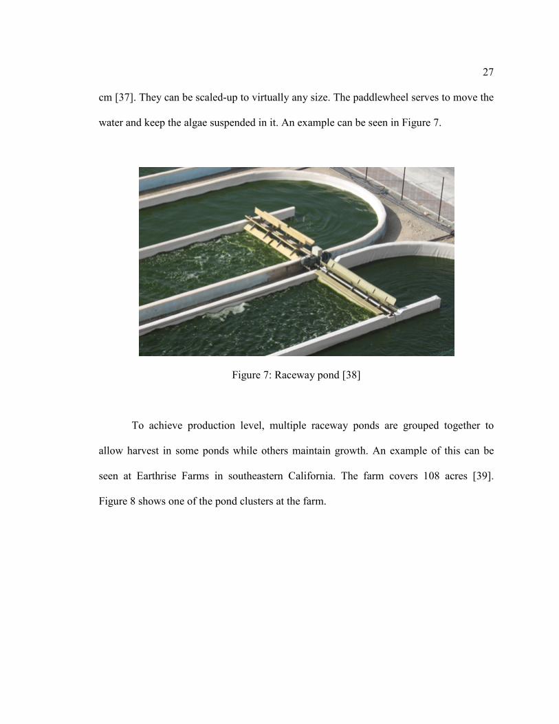
27 cm [37]. They can be scaled-up to virtually any size. The paddlewheel serves to move the

water and keep the algae suspended in it. An example can be seen in Figure 7.

Figure 7: Raceway pond [38]

To achieve production level, multiple raceway ponds are grouped together to

allow harvest in some ponds while others maintain growth. An example of this can be

seen at Earthrise Farms in southeastern California. The farm covers 108 acres [39].

Figure 8 shows one of the pond clusters at the farm.

28

Figure 8: Earthrise farm pond cluster [39]

Since commercial production is already accomplished this way, it makes sense to

design the harvest system around it. Mounting the cable suspended robot harvester at the

four corners of a pond cluster makes it possible to automatically harvest mature algae

communities while allowing others to grow. The robot can be programmed to harvest

specific locations at specific times across the pond cluster. For the sake of simplicity, all

simulations will be done assuming one pond, however, adaptation to multiple raceways is

a simple matter.

29

2. Thesis Objectives

The objective of this research is to incorporate a cable suspended robot harvesting

system into the current method of growing algae across large, commercial, open ponds.

This system will consist of four cables, which control the robot’s end-effector via four

winches, which are controlled independently, but simultaneously. This research includes:

• Kinematic, pseudostatic, and dynamic modeling of the proposed system

• The introduction of a novel approach to solving the forward pose kinematic

problem associated with cable robots

• Controller design proposal

• Robot design parameters, including:

o Tower specification

o Cable specification

o Mobility

o End effector suggestions

• MATLAB simulation, including examples

• Presentation of simulation results

30

3. Analysis

3.1 Definitions

In order to analyze this robot, it is necessary to establish frames and some

standard nomenclature. For this research, the English system of units is used, i.e., ft, lbf,

lbm, and sec. In this research, “ft” always stands for feet, “lbf” always stands for pounds-

force, “lbm” always stands for pounds-mass, and “sec” always stands for seconds. The

distinction between lbm and lbf must be noted here. “Lbm” is a unit of mass and “lbf” is

a unit of force. The simulation can be adopted for use with the metric system via small

alterations to the “define.m” MATLAB file. Figure 9 shows the variables chosen for this

model. These variables will be referenced throughout this paper.

Figure 9: Algae harvesting robot diagram, including nomenclature

P

XA

ZA YA

{A}

h2

L

W

h3

h4 h1

B2 B3

B4 B1

P2 P3

P4 P1

L2 L3

L4 L1

A1 A4

A3 A2

31

The base Cartesian reference frame is {A}, where the origin is located in the

center of the algae pond, at a h eight of zero. The coordinate axes XA, YA, and ZA are

shown in the figure. The harvest point is P. Since only position is being controlled with

this robot, the orientation of the platform is identical to {A}. A system can be added to

point P to control the orientation of the end effector. The cables are numbered from one

to four, clockwise from the lower left corner.

As shown in Figure 3, each cable is attached to a winch/reel at points Ai. The

cables pass over each telescoping tower at points Pi, which share the same x and y

coordinates as the pole bases, Bi, and have the z coordinates, hi. The Pi coordinates in the

{A} frame are:

{ }{ }{ }{ }

1 1

2 2

3 3

3 4

/ 2 / 2

/ 2 / 2

/ 2 / 2

/ 2 / 2

TA

TA

TA

TA

P L X W Y h

P L X W Y h

P L X W Y h

P L X W Y h

= − −∆ + ∆

= + ∆ + ∆

= + ∆ − −∆

= − −∆ − −∆

Where L and W are the rectangular dimensions of the pond, ΔX and ΔY are the x

and y offsets from the pond edges, and hi are the support pole heights.

The cable lengths are Li, as measured from Pi to P. This is the straight-line

distance, and does not take into account the catenary sag caused by the cable weight

and/or external forces.

This system has actuation redundancy since there are four cables controlling the

robot in three Cartesian coordinates. This redundancy, along with gravity’s effect on the

32 end effector and load, is used to maintain cable tension at all times. This is central to the

design due to the fact that cables can only be controlled using tension.

3.2 Workspace

In general, cable robot system workspaces are defined by two areas:

• Kinematic motion ranges and constraints, actuator limits, and cable

interference

• Demanding that all workspace operations require only cable tension to

maintain pseudostatic equilibrium

Cable interference will be eliminated by robot and controller design. Therefore,

the workspace will be limited, in general, to the area enclosed by the four support poles

since negative cable tension would be required to move outside the poles. In addition,

cable tensions tend to increase exponentially as the end effector approaches the

workspace boundaries, so the actual workspace is slightly smaller than the area enclosed

by the poles.

3.3 Kinematics

3.3.1 Inverse Pose Kinematics Analysis

The first step in analyzing this system is to perform the inverse pose kinematics

analysis. That is, given the position of the platform in the pond, determine the lengths of

the cables. Finding the cable length L can be found by taking the norm of the difference

between Bi and Pi in the {A} frame. The equation is:

i iL P P= −

or:

33

( ) ( ) ( )22 2i ix iy izL P x P y P z= − + − + −

3.3.2 Novel Forward Pose Kinematics Analysis

The forward pose analysis is much more difficult than the inverse pose analysis.

The forward pose problem statement is: given the cable lengths, determine the position of

the platform. This is a very challenging problem that requires the solution of coupled

non-linear equations. However, a simplified method for solving the forward pose

problem using the intersection of three spheres was proposed by R. L. Williams et al. in

2004 [34]. This approach involves setting the origins and radii of three spheres in the

system and finding where the spheres intersect. In this case, the origins are at the Bi and

the radii are Li. This problem is still moderately difficult to solve due to non-linear terms.

The approach can be seen in Figure 10.

Figure 10: Diagram of the three-spheres approach

34

A novel approach to this problem is shown below.

This system can be radically reduced by setting z1 = z2 = z3 as follows:

( ) ( ) ( )( ) ( ) ( )( ) ( ) ( )

2 2 2 21 1 1

2 2 2 22 2 2

2 2 2 23 3 3

n

n

n

x x y y z z r

x x y y z z r

x x y y z z r

− + − + − =

− + − + − =

− + − + − =

Where xn,yn, zn are the location of the tower tops and rn are the cable lengths.

Multiplying these out and subtracting equation 3 from one and two, the remaining

terms are:

( ) ( )

2 2 2 2 2 21 3 1 3 1 1 3 3 1 3

2 2 2 2 2 22 3 2 3 2 2 3 3 2 3

( 2 2 ) ( 2 2 )

2 2 2 2

x x x y y y x y x y r rx x x y y y x y x y r r

− + + − + + + − − = −

− + + − + + + − − = −

or:

ax by cdx ey f

+ =+ =

where:

1 3

1 32 2 2 2 2 2

1 3 1 1 3 3

2 3

2 32 2 2 2 2 2

2 3 2 2 3 3

2 22 2

2 22 2

bcd

a x xy y

r r x y x yx xy ye

r r x y x yf

=

= − − + +==

= − − +

= − +− +

−− +

+

− +

−

It then becomes possible to solve for x and y, since they are the only unknowns,

as z was eliminated in step one.

ce bfxae bd

−=

−

35

af cdyae bd

−=

−

Going back to the equation for the first sphere:

( ) ( ) ( )2 2 2 21 1 1nx x y y z z r− + − + − =

Since x and y are now known, the z component can be expanded z can be solved

for using the quadratic equation:

( ) ( )2 22 2 21 1 12 0n nz z z z x x y y r − + + − + − − =

2 4

2gg h

z±− ± −

Where:

( ) ( )2 22 21 1 1

2 n

n

g z

h z x x y y r

= −

= + − + − −

This will yield two values of z. It is easy to determine the correct z, however, as

one of the answers will invariably be above the height of the tower.

The unused sphere may be used to determine the accuracy of the solution by using

the inverse pose solution to find Li using the x,y,z values and comparing the results.

3.3.2.1 Example:

Let the tower positions be at the corners of a 200’x100’ rectangle, with a tower

height of 10 ft, and a harvest location of [50 25 0]:

[ ][ ][ ][ ]

1

2

3

4

100 50 10

100 50 10

100 50 10

100 50 10

P

P

P

P

= − −

= −

=

= −

36

Using the IPK solution:

( ) ( ) ( )22 2i ix iy izL P x P y P z= − + − + −

1

2

3

4

168.0030152.397556.789190.6918

LLLL

====

Therefore:

1

1

2

2

3

3

1

2

3

4

10050100

501005010

168.0030152.397556.789190.6918

n

xyxyxyzrrrr

= −= −= −========

Following the FPK solution from above:

( )( ) ( )( ) ( )( )( )( ) ( )( ) ( )( )( )( ) ( )( ) ( )( )

2 2 2 2

2 2 2 2

2 2 2 2

100 50 10 168.0030

100 50 10 152.3975

100 50 10 56.7891

x y z

x y z

x y z

− − + − − + − =

− − + − + − =

− + − + − =

Therefore:

( ) ( ) ( ) ( ) ( ) ( ) ( ) ( )( ) ( ) ( ) ( ) ( ) ( ) ( ) ( )

2 2 2 2

2 2 2 2

2 100 2 100 2 50 2 50 100 50 100 50 25000.0061

2 100 2 100 2 50 2 50 100 50 100 50 1999.9961

x y

x y

− − + + − − + + − + − − − =

− − + + − + + − + − − =

So:

37

40020025000400020000

bc

e

a

d

f

=====

=

So:

25000*0 200*20000 50.0000400*0 200*400

x −= =

−

400*20000 25000*400 25.0001400*0 200*400

y −= =

−

Going back to the equation for the first sphere:

( )( ) ( )( ) ( )2 2 2 250.0000 100 25.0001 50 10 168.0030z− − + − − + − =

( ) ( ) ( )2 22 2 2

2

2 10 10 150 75.0001 168.0030 0

20 0.0070 0

z z

z z

− + + + − = − + =

Solving for z:

20 400 4*0.00702

19.99960.0002

z

zz

±

+

−

± −=

== −

z+ is above the top of the tower and can be dismissed and z- is very nearly zero.

The slight deviation from zero can be eliminated by using more significant figures. This

result verifies the harvest position of [50 25 0]. As a further verification, the unused

equation for the fourth cable, ( ) ( ) ( )2 24 4 4

2 2nx x y y z z r− + − + − = can be used to check

the results.

38

( ) ( ) ( )( ) ( )( ) ( )

2 2 24 4 4

4

4

4

2

22 2 2

2

50.0000 100 25.0001 50 0.0002 1

2500 5625 100.004090.6 8

0

91

nx x y y z z r

r

rr

− + − + − =

− + − − + −

+ + ==

− =

Which is the correct length for the fourth cable.

3.3.3 Velocity Kinematics Analysis

The algae harvesting cable robot velocity kinematics analysis makes use of the

inverse pose solution, which is rewritten below, in its entirety.

( ) ( ) ( )22 2i ix iy izL P x P y P z= − + − + −

3.3.3.1 Inverse Velocity Kinematics Analysis

The inverse velocity kinematics problem is as follows: given the robot’s pose and

the desired velocity of the center of the platform, calculate the four cable rates.

The velocity equations come from the time derivative of the previous equation.

i i i ii

L L L Ldx dy dzLt x dt y dt z dt

∂ ∂ ∂ ∂= = + +∂ ∂ ∂ ∂

Where:

( ) ( ) ( )22 2

i ix

ix iy iz

L x Px P x P y P z

∂ −=

∂ − + − + −

( ) ( ) ( )22 2

iyi

ix iy iz

y PLy P x P y P z

−∂=

∂ − + − + −

( ) ( ) ( )22 2

i iz

ix iy iz

L z Pz P x P y P z

∂ −=

∂ − + − + −

39

Therefore:

iyix izi

i i i

y Px P z PL x y zL L L

−− −= + +

This can be written in the form:

{ } { }A AL J P =

Where AJ is the Jacobian matrix and { }AP is the velocity pose [40].

or:

11 1

1 1 1

21 2 2

2 2 22

33 3 3

3 3 34

44 4

4 4 4

yx z

yx z

yx z

yx z

y Px P z PL L L

y PL x P z Px

L L LLy

y PL x P z P zL L LL

y Px P z PL L L

− − − − − −

= −− − −− −

Cable velocities can be easily found using the precious equation.

3.3.3.2 Forward Velocity Kinematics Analysis

The forward velocity kinematics problem is as follows: given the robot’s pose and

cable rates, calculate the velocity of the center of the platform. In this case, however, the

problem is over-constrained due to having four equations and three unknowns. The

solution to this problem is:

{ } { }*A AP J L =

Where the over-constrained pseudoinverse is [40]:

40

( ) 1*A A T A A TJ J J J−

=

This is a s tandard method of finding a suitable inverse of an over-constrained

matrix. Extracting any three of the four equations and taking the standard inverse will

yield the same results. The fourth equation can be used to validate the results.

3.3.3.3 Velocity Singularities

Cable robots are subject to singularities when the determinant of the Jacobian

matrix equals zero, causing a divide-by-zero problem in the denominator. These

mathematical singularities are often signs of physical singularities such as exceeding the

workspace. The cable robot singularities can be found by solving:

0A T AJ J =

The solution to this problem exceeded MATLAB’s display capabilities, so a

simplification was done. As before, all tower heights were set to the same value, in this

case ‘h’. When the problem was again put to MATLAB and factored, the result was:

( ) ( )2

2 2 2 21 2 3 4

det B T B C h zJ J

L L L L−

=

Where C was an extremely long constant consisting only of Li, Piy, and Pix.

Setting this result to 0, the robot was found to be singular only when h = z. This proves

that singularities exist when the platform is equal to the tower height.

Interestingly, the statics singularities are identical to the velocity singularities.

This is due to the fact that the statics Jacobian is the negative transpose of the velocity

Jacobian [40].

41 3.3.4 Resolved-Rate Control Solution

The inverse velocity kinematics solution can be used as the basis for the resolved

rate control algorithm, which is an alternative control method for this robot. The resolved

rate method is useful if the user wants the platform to travel at a specific speed in the x,y,

and z coordinate system.

Using a given velocity input, the cable velocity { }L is calculated at each time

step using:

{ } { }A AL J P =

This information is then integrated to achieve{ }L . Next, the cable values are

inputted in each cable’s controller in order to achieve the desired motion.

3.3.5 Acceleration Kinematics Analysis

In order do the dynamics analysis of the system, the acceleration kinematics has

to be derived. In order to do this, the derivative of { }L is taken, giving:

{ } { } { }A A A AL J P J P = +

or:

{ }

11 1

1 1 11 1 1

22 2

2 2 2 2 2 2

33 3

3 3 3 3 3 3

44 4

4 4 4 4 4 4

yx z

yx z

yx z

yx z

y Px P z Px y zL L LL L L

y Px P z Px y zx

L L L L L LL y

x y z y Px P z PzL L L L L Lx y z y Px P z PL L L L L L

+ + − ++ −

= + ++ − ++ −

xyz

42 3.3.5.1 Inverse Acceleration Kinematics Solution

The previous solution leads to the inverse solution in a straightforward manner.

Given the robot’s pose configuration, velocity, and desired Cartesian acceleration, the

acceleration equation will give the cable acceleration, or { }L .

3.3.5.2 Forward Acceleration Kinematics Solution

The forward acceleration kinematics solution is not quite as straightforward as the

inverse. The problem is: given the robot pose configuration, velocity, and cable

acceleration, { }L , calculate the Cartesian acceleration. The equation for { }L must be

inverted to solve it. The inverted matrix is over-constrained, however, so the Moore-

Penrose pseudoinverse must again be used [40], giving:

{ } { } { }( )*A A A AP J L J P = −

3.3.6 Cable/Cable Reel Kinematics

In this section, the position, velocity, and acceleration kinematics for the

rotational to translational transformation of the active cable as they are spooled off the

reels is discussed. The solutions are straightforward, and can be achieved using geometry

and derivative calculus.

0i i i i

i i i

i i i

L r L

L r

L r

θ

θ

θ

• •

•• ••

= +

=

=

Where , ,i i iL L L• ••

are the cable length, velocity, and acceleration respectively, ri is

the reel radius, and , ,i i iθ θ θ• ••

are the reel angle, angular velocity, and angular acceleration.

43 L01 is the initial length of the cable, which is generally known as part of the calibration

process. This design is accurate only for reels where the cable does not wrap in layers.

3.4 Pseudostatics

Since the velocities of this cable robot system are relatively small and the weight

of the end effector will likely dominate the system, the robot can be analyzed using

pseudostatics. By this, it is assumed that the robot is in static equilibrium at every point

along its path of travel during its translation. For completeness, system dynamics will be

discussed in the next section.

3.4.1 Static Equilibrium

For the system to be in static equilibrium, the vector sum of the cable tensions, the

outside forces, and the weight of the end effector must be zero. The end effector weight

always acts down and includes the weight of the actual effector, as well as the weight of

the load being carried by it. When the end effector is underwater, the gravitational force

is reduced due to buoyancy, and the drag forces on i t are increased. The free-body

diagram of the end effector is shown in Figure 11.

Figure 11: Free-body diagram of cable robot end effector.

The force-only statics equations are:

t1

P

t2

t3 t3 W

F

44

{ } { } { } { }4

1

ˆ 0A A Ai i

it L F m g

=

+ + =∑

Where:

• ti is the cable tension along its cable length unit direction ˆAiL

• AF is the resultant force exerted on the platform by its environment

Under ideal conditions, F would be zero. It is included in this research to

accommodate external forces due to wind and water loading.

This equation may be represented in matrix form as:

{ } { } { }A A AA T F m g = − −

Where:

{ } { }1 2 3 4

1 2 3 4ˆ ˆ ˆ ˆ

T

A A A A A

T t t t t

A L L L L

=

=

From kinematics, ˆAiL can be determined as follows:

ˆ

A A Ai i

A A A AA i i

i A Aii

L P PP P P PL

LP P

= −

− −= =

−

iL was found earlier, in the IPK solution. When this is introduced, AA becomes

the statics Jacobian matrix:

45

1 2 3 4

1 2 3 4

1 2 3 4

1 2 3 4

31 2 4

1 2 3 4

x x x x

y y y yA

zz z z

P x P x P x P xL L L L

P y P y P y P yA

L L L LP zP z P z P z

L L L L

− − − − − − − −

= −− − −

One noteworthy piece of information is TA AA J = − . This is important

because only one of them needs to be calculated in a real-time control loop.

3.4.2 Forward Pseudostatics Solution

The forward pseudostatics solution is quite straightforward. Given the robot

configuration, the four cable tensions, and the end effector mass, the external force, AF ,

can be calculated using the following equation, from above:

{ } { } { }A A AF A T m g = − − (1)

3.4.3 Inverse Pseudostatics Solution

The inverse solution is slightly more difficult to derive than the forward solution,

but it is important. The problem is stated as follows: given the pose, end effector mass,

and external forces, AF , calculate the cable tensions, iT . The same equation from the

forward solution is used to derive the inverse, only it must be inverted to give the

solution. Since the matrix AA is not square, a plain inversion cannot be used. Since the

matrix is 3x4, this problem is under-constrained. This means that there are infinitely

many solutions to the problem since there are four cables and only three Cartesian

coordinates. This problem may be addressed by once again using the pseudoinverse of

the Jacobian [40]:

46

{ } { }†A AT A F mg = − +

Where:

( ) 1† T TA A A AA A A A−

=

These equations solve the inverse pseudostatics problem in such a way that the

Euclidian norm of the resulting cable tensions is minimized, which is an efficient method

for real-world simulation.

3.4.4 Singularities

Cable robots are subject to singularities, which are potential trouble

configurations in the workspace. A robot singularity occurs when the determinant of the

Jacobian matrix is zero, causing a divide-by-zero problem in the math, which is usually

accompanied by a physical problem such as loss or unwanted gain in freedom of end

effector movement. Problems can also occur in close proximity to singularities.

The cable-suspended robot singularity condition results from the following

determinant:

0TA AA A =

3.4.5 Cable Tension/Actuator Torque

In order to achieve the desired cable tensions to ensure static equilibrium with no

cable slack, actuator torques are the four control variables. Figure 12 shows the statics

free-body diagram for this torque via the cable reel.

47

Figure 12: Cable tension/actuator statics free-body diagram

Where τi is the actuator torque for joint i, ri is the cable reel radius, and ti is the

cable tension for cable i. This is most accurate for reels with a s ingle cable layer, as ri

changes as the cable wraps.

The cable tension/actuator statics transformation uses the cross product:

{ } { } { }i i ir tτ = ×

This solution only holds true for pseudostatics, due to reel inertia and robot

acceleration.

3.4.6 Translational Stiffness

Translational stiffness is the ability of a robot to resist translational deflections

when Cartesian forces,{ }AF , are exerted on it. High stiffness is desired in this case

because of the nature and task of the robot. The robot is outdoors and disturbances such

as waves and wind could push the robot off course. A stiffness study was first conducted

by Unger et al. in 1988 [41]. Translational stiffness units are lbf/ft, and rotational

stiffness units are (lbf-ft)/rad. The stiffness equation for the overall robot is [42].

[ ] TA A Ai diag

K A k A =

ti

ri

τi

48

Where AK is the 3x3 stiffness matrix, AA is the 3x4 forward pseudostatics

Jacobian matrix of the robot and and [ ]i diagk is a 4 x4 diagonal matrix, with diagonal

individual spring constant terms:

ii

EAkL

=

Where E is Young’s modulus of the cable material, A is the cross-sectional area,

and Li are the four cable lengths. The stiffness matrix diagonal terms are the stiffness of

the primary Cartesian components, x, y, and z and the other six terms represent the cross-

coupling directions. Translational stiffness depends on the end-effector position, via the

Jacobian matric, and the cable lengths. Although the stiffness matrix is relatively easy to

calculate, there is some difficulty in evaluation and comparison. In order to standardize

and simplify, the three eigenvalues of the matrix are extracted. These eigenvalues

represent the principal stiffness components and the eigenvectors will give the directions

of these stiffness values. If further simplification is required, the Euclidian norm of the

three principal values will give a single stiffness value in lbf/ft.

3.5 Dynamics

Dynamics is the study of motion with regard to forces. Dynamics modeling is

important for large outdoor cable robot systems wherein large velocities and

accelerations are required. Dynamics modeling is also required for the design of cable

robot controllers because it helps determine the characteristics of designed controllers

before implementation.

49 3.5.1 Dynamics Equations of Motion

In this section, dynamics modeling is presented. These equations are used to

simulate overall system dynamics and to calculate the cable tensions, and hence actuator

torques, to provide dynamic motions in all robotic configurations. Dynamics depend on

knowing all kinematics variables for all motion.

Figure 13 shows the dynamics free-body diagram for the robot, assuming the end

effector is a point mass with no rotation.

Figure 13: Dynamics free-body diagram

The diagram is identical to the one presented in the pseudostatics section of this

document.

For dynamics modeling, Newton’s second law is used:

{ } { }A AF m P=∑

The summation of forces involves the vector sum of the four active cable tensions

exerted on the end effector, the external forces, and the total end-effector weight.

Generally, for highly dynamic motions with large velocities and accelerations, it is not

t1

P

t2

t3 t3 W

F

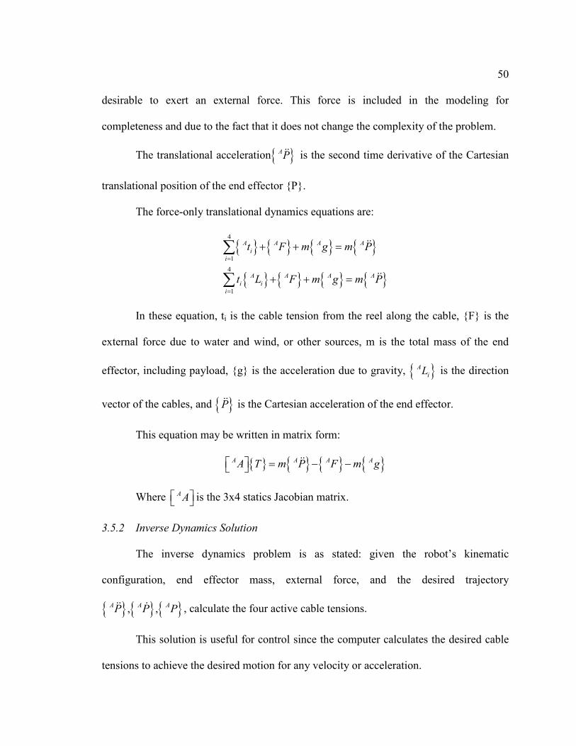
50 desirable to exert an external force. This force is included in the modeling for

completeness and due to the fact that it does not change the complexity of the problem.

The translational acceleration{ }AP is the second time derivative of the Cartesian

translational position of the end effector {P}.

The force-only translational dynamics equations are:

{ } { } { } { }

{ } { } { } { }

4

14

1

A A A Ai

i

A A A Ai i

i

t F m g m P

t L F m g m P

=

=

+ + =

+ + =

∑

∑

In these equation, ti is the cable tension from the reel along the cable, {F} is the

external force due to water and wind, or other sources, m is the total mass of the end

effector, including payload, {g} is the acceleration due to gravity, { }AiL is the direction

vector of the cables, and { }P is the Cartesian acceleration of the end effector.

This equation may be written in matrix form:

{ } { } { } { }A A A AA T m P F m g = − −

Where AA is the 3x4 statics Jacobian matrix.

3.5.2 Inverse Dynamics Solution

The inverse dynamics problem is as stated: given the robot’s kinematic

configuration, end effector mass, external force, and the desired trajectory

{ } { } { }, ,A A AP P P , calculate the four active cable tensions.

This solution is useful for control since the computer calculates the desired cable

tensions to achieve the desired motion for any velocity or acceleration.

51 Using the matrix form of the dynamics equation, the need for the pseudoinverse

arises again due to the fact that AA is not a square matrix, giving:

{ } { } { } { }( )†A A A AT A m P F m g = − −

Where †AA is the pseudoinverse [40]:

( ) 1† T TA A A AA A A A−

=

It is possible to use this method to optimize additional constraints. Although the

weight of the end effector and load will general keep the cables taut under pseudostatic

conditions, conditions may arise when end effector acceleration may cause the cables to

go slack. Simulation must be done in order to find the acceleration at which this happens

to avoid problems with the system.

3.5.3 Forward Dynamics Solution

The forward kinematics problem is as stated: given the robot’s kinematic

configuration, end effector mass, external force, and the active cable tensions, calculate

the motion { } { } { }, ,A A AP P P of the robot.

This solution is useful for simulation of dynamic motion, especially to evaluate

the performance of a designed controller prior to implementation.

Using the dynamics equation again and solving for { }AP , the solution is:

{ } { } { } { }( )1A A A AP A T F m gm

= + +

Velocity and acceleration can be found by numerically integrating the results of

the previous equation.

52 3.5.4 Actuator/Cable Reel Dynamics

Deriving the dynamics equations for a single actuator/cable reel is important for

designing a proportional-integral-derivative (PID) controller for the system. Following

standard industrial practice, it is generally effective to control all cable lengths

independently, but simultaneously.

First, the general dynamics model for a DC motor driving a cable reel will be

derived. Then some simplifications will be introduced to achieve an acceptable dynamics

model for the PID controller.

Figure 14 shows the diagram for an actuator with its cable reel and cable,

connected to the end effector of mass m.

Figure 14: Single actuator/cable reel diagram

The brush DC motor is activated by an armature circuit with input voltage v(t),

current i(t) back emf vB(t), plus constant inductance and resistance coefficients L and R.

v(t) n

ri

ω(t) Li

m*

i(t) vB(t)

53 The motor torque τ(t) in generated via the circuit current, rotating the motor shaft relative

to the stator. The cable reel, radius r, is rotated through the gear ratio n. In turn, the cable

reel changes the cable length L, which is attached to the end effector, of mass m. Since

there are four cables supporting the end effector, each will bear a fraction of the weight.

For simplification, the fraction borne by each cable will be taken as a constant m*.

The armature circuit dynamic model is a first order ordinary differential equation:

( ) ( ) ( ) ( )Bdi tL Ri t v t v tdt

+ = −

The electromechanical coupling equations are proportional algebraic equations:

( ) ( )( ) ( )B

i Ki tv t K tτ

ω==

Where the motor torque τ(t) is proportional to the circuit by a torque constant K

and the back emf voltage vB(t) is proportional to the shaft angular velocity ω(t) by the

same constant.

Making two standard simplifications make this system much more manageable.

First, the electrical circuit first order rise time constant is usually much faster than the

mechanical rotational system first order time constant. Therefore, the inductor will not

have enough time to full charge. This means the inductance value can be assumed to be 0.

Second, the back emf voltage will be ignored for the sake of simplicity.

This simplifies the armature dynamic model from an ODE to a proportional

equation:

( ) ( )Ri t v t=

54

Figure 15 shows the free-body diagram for the mechanical portion of the

actuator/cable reel.

Figure 15: Actuator/cable reel free-body diagram

Where the motor shaft and cable reel mass moment of inertia are lumped into one

constant J, the rotational viscous damping coefficient is c, the torque applied to the reel

shaft is nτ(t) where n is the gear ratio, the cable tension is t(t), and the cable reel shaft

angle is θCR(t). The gear ratio relationships are:

( ) ( )( ) ( )

CR

CR

t tnt t

τ θτ θ

= =

Where the CR subscript indicates the cable reel shaft torque and no s ubscript

indicates the motor shaft torque.

For the cable reel dynamics model, Euler’s Rotational Dynamics Law is used:

( )

( ) ( ) ( ) ( )E CR CR

M J t

n t c t rt t J t

α

τ θ θ

=

− − =

∑

m*

t(t)

nτ(t) JE

𝒄𝑬�̇�𝑪𝑹

55

Where the angular acceleration of the cable reel shaft is ( ) ( )CRt tα θ= and the

effective rotational viscous damping coefficient is represented at the shaft as cE.

For the partial mass m* translational dynamics model, Newton’s second law is

used:

* ( )( ) * ( )

F m a tt t m x t

=

=∑

Where the translational acceleration of the cable reel shaft is ( ) ( )a t x t= . The

following relationships between cable reel rotation and cable length change also exist:

( ) ( )

( ) ( )

( ) ( )

CR

CR

CR

x t r t

x t r t

x t r t

θ

θ

θ

=

=

=

Combing Euler’s equation with Newton’s equation and the rotational

relationships gives the following second order ODE model for the mechanical portion of

the cable reel system:

( )2* ( ) ( ) ( )CR E CRJ m r t c t n tθ θ τ+ + =

Finally, combining the mechanical and electrical models gives the following:

( )2* ( ) ( ) ( )CR E CRnKJ m r t c t v tR

θ θ+ + =

Applying the Laplace transformation:

( )

( )

2 2

2 2

( ) * ( ) ( )

( ) * ( )

CR CR E

CR E

nKs s J m r s s c V sR

nKs J m r s c s V sR

Θ + + Θ =

Θ + + =

56

The associated open loop transfer function from the previous equation for a single

joint PID controller design is:

( ) ( ) ( )2 2

( )( )( ) * E E E EE

s nK nK bG sV s Rs J s c s J s cR J m r s c sΘ

= = = =+ + + +

Where the effective rotational inertia of the cable reel /motor shaft is

2EJ J mr= + and nKb

R= is a system constant defined for convenience.

This result will be used in the following section to design the controller for the

system.

3.6 PID Controller Design

This section presents PID controller design applied to each joint of the proposed

cable-suspended robot. This is for independent, but simultaneous, control of all four

cables for coordinated motion. The standard system block diagram used in this design is

shown in Figure 16.

57

Figure 16: Single input, single output, negative feedback closed loop block diagram

The open-loop transfer function for this design was derived in the previous

section:

( )( )

E E

bG ss J s c

=+

Including a controller function Gc(s) and a sensor transfer function H(s), the

resulting standard closed-loop transfer function T(s) is given below:

( ) ( )( )( )( ) 1 ( ) ( ) ( )

c

c

G s G sY sT sR s G s G s H s

= =+

Using the open-loop transfer function derived above, the standard PID transfer

function Gc(s), and assuming a p erfect sensor (H=1), the closed-loop transfer function

derivation is:

58

( )

( )

( )

( ) 1

Ic P D

E E

KG s K K ss

bG ss J s c

H s

= + +

=+

=

( )

( )

( ) ( ) ( )

( ) ( ) ( )

2

2

( ) ( )( )1 ( ) ( ) ( )

( )1 1

( )1

( )

c

c

IP D

E E

IP D

E E

P I D

E E E E E E

P I D

E E E E E E

P I

G s G sT sG s G s H s

K bK K ss s J s c

T sK bK K ss s J s c

K b K b K bs J s c s J s c J s c

T sK b K b K b

s J s c s J s c J s c

K bs K

T s

=+

+ + + = + + + +

+ + + + + =

+ + + + + +

+

=( )

( )

( )( )( ) ( )

( )( )

2

2

2

2

2

2

2 2

2 2

2

2

2

1

( )

( )

D

E E

P I D

E E

P I D

E E

E E P I D

E E E E

P I D

E E

E E P I D

b K bss J s c

K bs K b K bss J s c

K bs K b K bss J s c

T ss J s c K bs K b K bss J s c s J s c

K bs K b K bss J s c

T ss J s c K bs K b K

+ + + +

+ + + + + =

+ + ++ + +

+ + + =+ + + +

( )( )

( ) ( ) ( )

2

2

2

3 2( )

E E

D P I

E E D P I

bss J s c

b K s K s KT s

J s c bK s bK s bK

+

+ +=

+ + + +

59 For controller design, it is convenient to normalize the denominator of the above

equation so that the leading coefficient of the characteristic equation is 1. This is shown

in the following equation:

( )

( ) ( ) ( )

2

3 2

( )

D P I

E

E D P I

E E E

b K s K s KJT s

c bK bK bKs s s

J J J

+ +

=+

+ + +

The basis of controller design via denominator matching is to match the symbolic

form of the T(s) denominator with the numerical desired characteristic polynomial, since

it is well known that the nature of the roots of the denominator determine the nature of

the transient response. Given that there are many methods to determine good system

behavior, for now only the form of the desired characteristic polynomial is given:

3 22 1 0( )DES s s a s a s a∆ = + + +

To solve for the unknown controller gains KP, KI, and KD, the denominator of the

derived transfer function T(s) will be matched to ΔDES(s):

( )

( )

( )

3

22

11

00

1

E D

E

P

E

I

E

sc bK

s aJ

bKs a

JbK

s aJ

→

+→ =

→ =

→ =

Therefore, the PID controller solution is:

60

2

1

0

E ED

EP

EI

J a cKb

J aKb

J aKb

−=

=

=

The previous solution guarantees correct behavior of the denominator in the

closed-loop system, however, it introduces an unwanted numerator that will change the

transient response by adding unwanted zeros in the numerator. This problem is easily

remedied by using a pre-filter function GP(s) before the summing junction in Figure 9.

This pre-filter function is given below:

( )

( ) 22( )

I

E IP

D P ID P I

E

bKJ KG s

K s K s Kb K s K s KJ

= =+ ++ +

Since the values of n, K, R, JE, and cE are dependent on the winch used, they will

be determined later. For now, this PID controller design will continue to use variables.

The controller designer always needs to choose the desired behavior of the closed-

loop system; this is called dynamics shaping. In order to define the system behavior, the

closed-loop polynomial (ΔDES) must be defined. Although there are many methods to do

dynamic shaping, this research focuses on t he standard underdamped generic second

order system resulting from a unit step input.

Using the standard equations:

61

21

2 2

1004

( ) 2

sn

DES n n

PO e

t

s s s

ξπ

ξ

ξω

ξω ω

− − =

≅

∆ = + +

Where PO is percent overshoot, ξ is the damping ratio, ts is the settling time, ωn is

the approximate natural frequency, and ΔDES is the desired closed-loop characteristic

polynomial.

From PO, it is possible to calculate ξ:

( )( )

21

2

2 2 2 2

2 2 2 2

2

2 2

100

ln100 1

1

PO

PO

PO PO

PO

PO

PO ePOL

L

L L

LL

ξπ

ξ

ξπ

ξ

ξ ξ π

ξ π

ξπ

− − =

− = = −

− =

+ =

= ++

From this point, it is possible to calculate ωn:

4

4

sn

ns

t

t

ξω

ωξ

≅

≅

Substituting into the desired characteristic polynomial:

62

( )

2 2

222

2 2

2 22

2 2

( ) 2

4 4( ) 2

168( )

DES n n

PODES

PO s s

PODES

s PO s

s s s

Ls s sL t t

Ls s s

t L t

ξω ω

π ξ ξ

π

∆ = + +

∆ = + + +

+∆ = + +

In order to match this polynomial with the third-order polynomial needed for this

controller, a third pole, s3, must be introduced. The standard method for doing this is to

take the real part of the dominant second order poles, and include it as a real, negative,

10x third pole. Since doing this symbolically would be messy, an example is included to

clarify the method.

3.6.1 Potential Errors and Disturbances

While, by design, the PID controller inherently controls most disturbances and

deviations from the desired system response, extra steps must be taken to ensure proper

system operation in the event of error. Since the system relies on proper cable tension to

function, inline tension meters should be installed in case of cable slack or breakage. In

addition, an accurate GPS device could be attached to the end effector to collaborate the

position and velocity of the harvester. This backup check would help in the case where

the cables became snagged or tangled as well, and could alert the device operator of

errors.

3.6.2 Design Example

Assuming a PO of 5% and ts of 1.5s, the resultant values are:

63

( )

( )

2 22

2 2

22

2

168( )

16 8.97448( )1.5 8.9744*2.25

( ) 5.3333 14.9316

PODES

s PO s

DES

DES

Ls s s

t L t

s s s

s s s

π

π

+∆ = + +

+∆ = + +

∆ = + +

The roots of which are 2.6667 2.7965i− ± . Therefore, the third pole is

3 26.6667s = − .

The resulting closed-loop characteristic polynomial is now third order:

( )( )3

3

2

3 2

( ) 26.6667 5.3333 14.9316

( ) 32 157.2 398.2DES

DES

s s s s

s s s s

∆ = + + +

∆ = + + +

From above, the form of the desired polynomial is:

3 22 1 0( )DES s s a s a s a∆ = + + +

Where:

( )

( )

( )

3

22

11

00

1

E D

E

P

E

I

E

sc bK

s aJ

bKs a

JbK

s aJ

→

+→ =

→ =

→ =

Therefore:

64

( )

( )

( )

2

1

0

32

152.2

398.2

E D

E

P

E

I

E

c bKa

JbK

aJ

bKa

J

+= =

= =

= =

So:

32

152

398.2

E ED

EP

EI

J cKb

JKb

JKb

−=

=

=

Depending on the characteristics of the winch, these values are used to find the

transfer function and pre-filter using the equations given previously:

( )

( ) ( ) ( )

2

3 2

( )

D P I

E

E D P I

E E E

b K s K s KJT s

c bK bK bKs s s

J J J

+ +

=+

+ + +

2( ) IP

D P I

KG sK s K s K

==+ +

65

4. Simulation & Design Decisions

In this chapter, MATLAB was used to simulate the cable suspended robot in order

to verify derivations and determine some design parameters for the system. The

following constants were used for this simulation: 1 acre pond with a rectangular shape

that follows the golden ratio, or φ ≈ 1.618:1, with W ≈ 164.1 ft and L ≈ 265.5 ft. The four

telescoping poles had a height of 10 ft, and were set away from the pond edges a distance

of 5 ft in the x and y directions. The combined mass of the end effector and algae payload

was estimated to be 100 lbm. For stiffness calculations, a cable diameter of ½ inch was

used, with a modulus of elasticity of 29,000,000 lbf/in2. Figure 17 shows an example of

the output from the program, showing a one acre pond with 10 ft tall towers, where the

end effector is at the staging/calibration area.

Figure 17: MATLAB simulation of the proposed system

-100

-50

0

50

100

-50

0

50

0510

66 4.1 Snapshot Examples

Given the above constants and a harvest position of [0 0 0] , the MATLAB

simulation returned the following results using the math derived previously:

1 2 3 4

1 2 3 4

163.2440408.1099

L L L L ftT T T T lbf

= = = == = = =

Figure 18 shows the simulation returned from the program:

Figure 18: Center point snapshot simulation

When the active lengths were applied to the forward pose kinematic (FPK)

solution supplied above, the results were as follows:

[ , , ] [0,0,0]x y z =

This proved the results from the inverse pose kinematic solution (IPK) were

accurate.

As a secondary check, the system was given the initial coordinates of: [40 -30 4].

Figure 19 is from the simulation.

-100-50

050

100

-50

0

50

0510

67

Figure 19: Snapshot example at [40 -30 4]

The results of the snapshot were:

1

2

3

4

1

2

3

4

186.7662212.8997152.6027113.3265678.2294485.8180485.1462858.3550

L ftL ftL ftL ftT lbfT lbfT lbfT lbf

========

Inputting the results back into the FPK solution yielded:

[ , , ] [40, 30,4]x y z = −

Once again, this solution verified the results.

4.2 Single Point Harvest

-100-50

050

100

-50

0

50

0510

68

Figure 20: End effector at the staging area for a 1 acre pond

Figure 21: End effector at a harvest location of [60 40 0]

-100-50

050

100

-50

0

50

0510

-100-50

050

100

-50

0

50

0510

69

Figure 22: Cable lengths as a function of time steps for a single harvest

Figure 23: End effector position as a function of time steps for a single harvest

0 20 40 60 80 100 12080

100

120

140

160

180

200

220

240

Time Steps

Leng

th (f

t)

L1L2L3L4

0 20 40 60 80 100 120-100

-80

-60

-40

-20

0

20

40

60

Time Steps

Pos

ition

(ft)

xyz

70

Figure 24: Cable velocities as a function of time steps for a single harvest

Figure 25: Cable tensions as a function of time steps for a single harvest

0 20 40 60 80 100 120-5

-4

-3

-2

-1

0

1

2

3

4

5

Time Steps

Cab

le V

eloc

ity (f

t/s)

Ld1Ld2Ld3Ld4

0 20 40 60 80 100 1200

200

400

600

800

1000

1200

1400

Time Steps

Cab

le T

ensi

on (l

bf)

T1T2T3T4

71

Figure 26: Stiffness norm as a function of time steps for a single harvest

Max: 1358.8 lbf

4.3 Corner to Corner Harvest

Figure 27: End effector at the start of a corner-to-corner trajectory

0 20 40 60 80 100 1208.5

9

9.5

10

10.5

11x 10

4

Time Steps

Eig

enva

lue

norm

(lbf

/ft)

-100-50

050

100

-50

0

50

0510

72

Figure 28: End effector at the end of a corner-to-corner trajectory

Figure 29: Cable lengths as a function of time steps for a corner-to-corner trajectory

-100-50

050

100

-50

0

50

0510

0 10 20 30 40 50 60 70 80 90 1000

50

100

150

200

250

300

350

Time Steps

Leng

th (f

t)

L1L2L3L4

73

Figure 30: End effector position as a function of time for a corner-to-corner trajectory

Figure 31: Cable velocities as a function of time for a corner-to-corner trajectory

0 10 20 30 40 50 60 70 80 90 100-150

-100

-50

0

50

100

150

Time Steps

Pos

ition

(ft)

xyz

0 10 20 30 40 50 60 70 80 90 100-5

-4

-3

-2

-1

0

1

2

3

4

5

Time Steps

Cab

le V

eloc

ity (f

t/s)

Ld1Ld2Ld3Ld4

74

Figure 32: Cable tensions as a function of time for a corner-to-corner trajectory

Figure 33: Stiffness norm as a function of time for a corner-to-corner trajectory

0 10 20 30 40 50 60 70 80 90 1000

200

400

600

800

1000

1200

1400

Time Steps

Cab

le T

ensi

on (l

bf)

T1T2T3T4

0 10 20 30 40 50 60 70 80 90 1000.5

1

1.5

2

2.5

3

3.5

4

4.5x 10

5

Time Steps

Eig

enva

lue

norm

(lbf

/ft)

75 4.4 Tower Choice

It is important that the tower is: adjustable to equalize z – height, mobile, sturdy

enough to withstand the forces on t he system, and rugged enough to withstand the

elements. There are many towers available commercially. Their marketed uses include

communication, military, emergency, and mobile lighting and sound systems. Most

variations involve a lattice or tube structure that is raised by pulleys and winches and

stabilized by arms that pivot away from the main body and secure to the ground.

Although the option exists to mount the towers to vehicles, the system will be a semi-

permanent fixture in this research. Therefore, the trailer type tower will be considered

primarily.

One example of these mobile towers, made by Aluma Tower Company, Inc., can

be found in Figure 34.

76

Figure 34: Scorpion® tower from Alumina Tower Company, Inc. [43]

4.5 Appropriate Tower Height

Since it is known that the cable tension will increase toward infinity as the end

effector approaches the height of the towers, a program was written to simulate the

system pseudostatics as a load is raised vertically at different points, pond sizes, tower

heights, and loads. The simulation sets the origin of the end effector at 0 ft, level with the

bottom of the towers, and raises it to 90% of the tower height to avoid singularities. It

does not take into account the size of the end effector and must be edited when an

appropriate harvest tool is chosen. This program can be found in the appendix. The

77 program operated using the pseudostatics derivation provided earlier and a constant step

size in the z-direction.

This simulation finds the height at which the cable tension is three times the

tension at a height of zero. This height, expressed as a percentage of tower height,

provides a reasonable estimate of the maximum height to which a load should be raised,

based on plot trends from trial and error experimentation. At three times the base tension,

the cable tensions are universally still far from approaching infinity toward the beginning

of the exponential trend. Although this method is not as accurate as accounting for

dynamics, it provides a reasonable response for determining general tower height. Figure

35 shows a pond of one acre, with the load of 100 lbm in the middle of the pond, being

raised to a tower height of 10 ft. This will be the standard device configuration.

Figure 35: Standard pond setup with a center point harvest and 10 ft towers

-100-50

050

100

-50

0

50

0510

78

Figure 36: 1 acre pond, center harvest, 100 lbm, 10 ft towers, and vertical lift

It can be seen from Figure 36 that all cable tensions were equal since the end

effector was in the center of the pond. The output from the simulation gave a 3x height of

6.73 ft, or 67.3% of tower height for all cables.

Using the same pond configuration and increasing the tower height to 20 ft gave

the following results.

0 1 2 3 4 5 6 7 8 90

500

1000

1500

2000

2500

3000

3500

4000

4500

Height (ft)

Tens

ion

(lbf)

T1T2T3T4

79

Figure 37: Standard pond setup with a center point harvest and 20 ft towers

Figure 38: 1 acre pond, center harvest, 100 lbm, 20 ft towers, and vertical lift

-100-50

050

100

-50

0

50

01020

0 2 4 6 8 10 12 14 16 18200

400

600

800

1000

1200

1400

1600

1800

2000

2200

Height (ft)

Tens

ion

(lbf)

T1T2T3T4

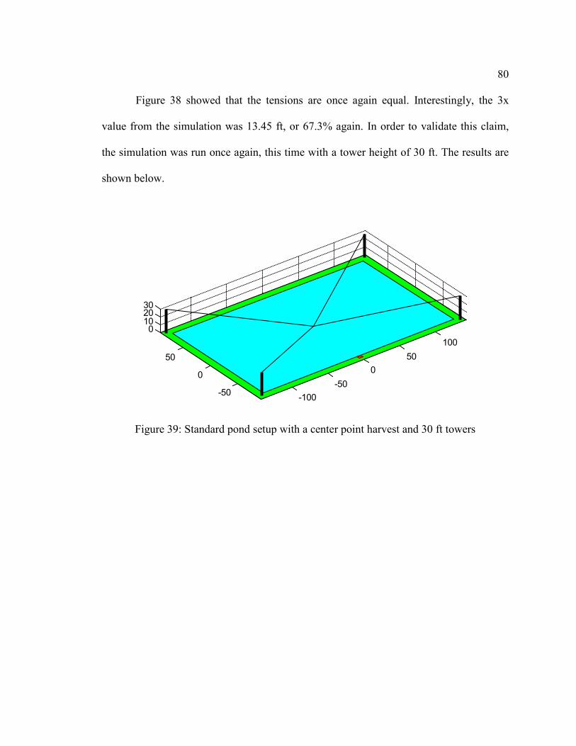
80 Figure 38 showed that the tensions are once again equal. Interestingly, the 3x

value from the simulation was 13.45 ft, or 67.3% again. In order to validate this claim,

the simulation was run once again, this time with a tower height of 30 ft. The results are

shown below.

Figure 39: Standard pond setup with a center point harvest and 30 ft towers

-100-50

050

100

-50

0

50

0102030

81

Figure 40: 1 acre pond, center harvest, 100 lbm, 30 ft towers, and vertical lift

Once again, this result verified the trend. The tensions were again equal and the

3x value was 20.18 ft, or 67.3% again.

The next issue to discuss becomes that of harvest location. It is necessary to

determine how the cable tensions change as the location of the end effector changes. The

simulation was run at different points in the same one acre point, with a fixed tower

height of 10 ft, and a load of 100 lbm, with a vertical lift. Figure 41 shows the same one

acre pond, with a harvest point of [60, 40].

0 5 10 15 20 25 300

200

400

600

800

1000

1200

1400

Height (ft)

Tens

ion

(lbf)

T1T2T3T4

82

Figure 41: Standard pond setup with a [60 40] harvest and 10 ft towers

Figure 42: 1 acre pond, [60, 40] harvest, 100 lbm, 10 ft towers, and vertical lift

-100-50

050

100

-50

0

50

0510

0 1 2 3 4 5 6 7 8 90

1000

2000

3000

4000

5000

6000

Height (ft)

Tens

ion

(lbf)

T1T2T3T4

83

Although the tensions were no longer identical, they still maintained a 3x point of

6.73 ft or 67.3% of tower height. This result was identical to the results from the center

harvest.

Figure 43 shows a harvest location of [-130, -80], which is near the edge of the

pond.

Figure 43: Standard pond setup with a [-130 -80] harvest and 10 ft towers

-100-50

050

100

-50

0

50

0510

84

Figure 44: 1 acre pond, [-130, -80] harvest, 100 lbm, 10 ft towers, and vertical lift

From the simulation, while the 3x points had changed slightly, the values were:

1 75.5%2 67.3%3 66.4%4 68.2%

====

Which were still close to the values for the center harvest.

In order to ensure the same tension response for all situations, the system was

modeled again using different sized ponds and with different payloads. Figure 45 shows a

100’x100’ pond with 10 ft tall towers, a center harvest, and a load of 100 lbm.

0 1 2 3 4 5 6 7 8 90

100

200

300

400

500

600

700

800

900

1000

Height (ft)

Tens

ion

(lbf)

T1T2T3T4

85

Figure 45: 100’x100’ pond with a center harvest and 10 ft towers

Figure 46: 100’x100’ pond, center harvest, 100 lbm, 10 ft towers, and vertical lift

-60-40

-200

2040

60

-60-40

-200

2040

6005

10

0 1 2 3 4 5 6 7 8 90

200

400

600

800

1000

1200

1400

1600

1800

2000

Height (ft)

Tens

ion

(lbf)

T1T2T3T4

86 Once again, the tension trend followed the same pattern of 67.3% of tower height.

Finally, to fully ensure the system behaves the same under all conditions, the load

was varied on the standard pond from 50 lbm to 200 lbm. The following figures show the

results.

Figure 47: 1 acre pond, center harvest, 50 lbm, 10 ft towers, and vertical lift

0 1 2 3 4 5 6 7 8 9200

400

600

800

1000

1200

1400

1600

1800

2000

2200

Height (ft)

Tens

ion

(lbf)

T1T2T3T4

87

Figure 48: 1 acre pond, center harvest, 200 lbm, 10 ft towers, and vertical lift

Once again, the system behaved as expected with a 3x height of 67.3%.

As a final test, the tower height was incrementally increased from 0 t o 100 ft,

using a center harvest and 50 and 100 lbm loads at a harvest height of zero ft. In this

simulation, the tension at the maximum towers height was calculated first, and the height

at which the tensions were 3x the minimum tension were found to benchmark the results.

The following figures show the results.

0 1 2 3 4 5 6 7 8 90

1000

2000

3000

4000

5000

6000

7000

8000

9000

Height (ft)

Tens

ion

(lbf)

T1T2T3T4

88

Figure 49: 1 acre pond, center harvest, 100 lbm, and varying tower height

As seen in the figure, the tension started high and quickly decreased. For the

standard pond setup, the 3x point was found to be at 18 ft.

0 10 20 30 40 50 60 70 80 90 1000

500

1000

1500

2000

2500

3000

3500

4000

4500

Tower Height (ft)

Cab

le T

ensi

on (l

bf)

T1T2T3T4

89

Figure 50: 1 acre pond, center harvest, 50 lbm, and varying tower height

The tension curve followed the same shape, with a 3x height of 18 ft, once again.

The pond size was changed to a half acre and the simulation was performed again.

0 10 20 30 40 50 60 70 80 90 1000

500

1000

1500

2000

2500

Tower Height (ft)

Cab

le T

ensi

on (l

bf)

T1T2T3T4

90

Figure 51: ½ acre pond, center harvest, 100 lbm, and varying tower height

In this case, the 3x height was found to be 16 ft.

Figure 52: 100’x100’ pond, center harvest, 100 lbm, and varying tower height

0 10 20 30 40 50 60 70 80 90 1000

500

1000

1500

2000

2500

3000

Tower Height (ft)

Cab

le T

ensi

on (l

bf)

T1T2T3T4

0 10 20 30 40 50 60 70 80 90 1000

200

400

600

800

1000

1200

1400

1600

1800

2000

Tower Height (ft)

Cab

le T

ensi

on (l

bf)

T1T2T3T4

91

For the 100’x100’ pond, the 3x point was found to be 13 ft.

Figure 53: 10’x10’ pond, center harvest, 100 lbm, and varying tower height

For the 10’x10’ pond, the 3x point was found to be 3 ft.

0 10 20 30 40 50 60 70 80 90 1000

50

100

150

200

250

300

350

400

Tower Height (ft)

Cab

le T

ensi

on (l

bf)

T1T2T3T4

92

From the above simulations, it can be observed that cable tensions decreased

rapidly as tower height increases. From multiple tests, it can be seen that the 3x criteria

was useful in determining proper height since it approached the exponential region in

every case. For most cases (with the exception of the 10’x10’ pond, which is likely too

small an area to be useful), the 3x point fell between 10 and 20 ft. This test was useful

because it showed that since tension decreases so rapidly, proper tower height is

primarily a function of maximum load height.

Dividing 1 by 0.673 shows tower height should be at least approximately one and

a half times the height of the highest point on the harvest trajectory. The highest point on

the trajectory is determined by the robot’s configuration, including pond and end effector,

which will be discussed later. This height can be controlled by the PID controller of the

robot.

4.6 Cable Choice

Cable choice is greatly dependent on r obot design. The cable must be strong

enough to withstand the forces applied to it by the end effector, the robot’s motion, and

any outside forces. The cables must also be as light as possible due to the long spans

needed for implementation. In addition, the lines will be outside and exposed to wet

conditions and must therefore be resistant to oxidation.

It is for these reasons that synthetic rope is preferable to metal rope. Synthetic

rope can be as strong as steel at a tenth of the weight [44]. It is also immune to rust and is

being used worldwide for marine applications. One type of synthetic rope being

considered currently is Novabraid® Spectec-12. In addition to the desired qualities

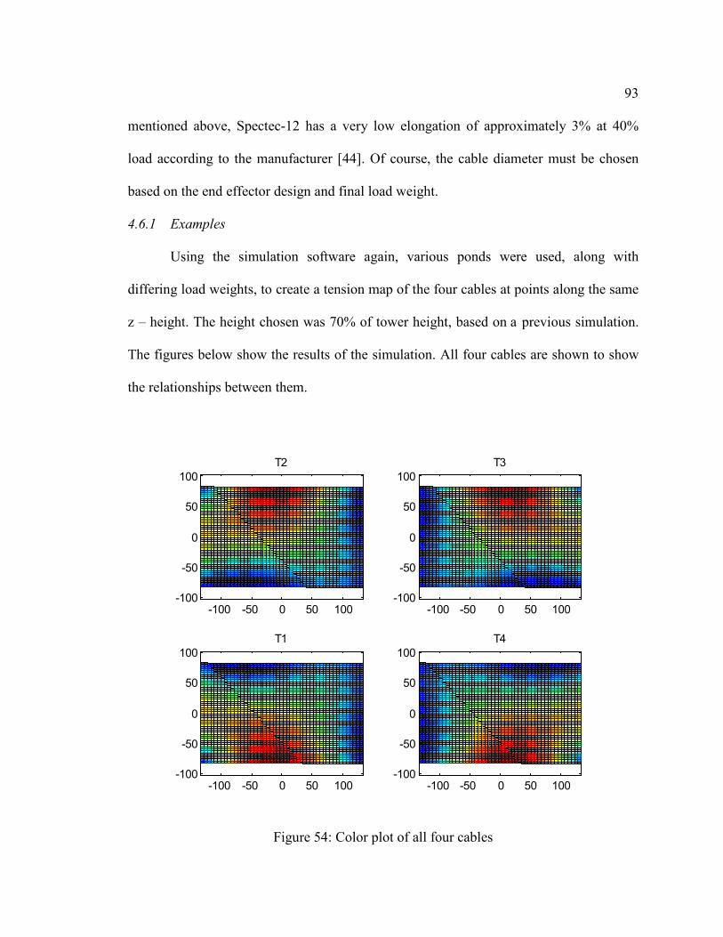
93 mentioned above, Spectec-12 has a very low elongation of approximately 3% at 40%

load according to the manufacturer [44]. Of course, the cable diameter must be chosen

based on the end effector design and final load weight.

4.6.1 Examples

Using the simulation software again, various ponds were used, along with

differing load weights, to create a tension map of the four cables at points along the same

z – height. The height chosen was 70% of tower height, based on a previous simulation.

The figures below show the results of the simulation. All four cables are shown to show

the relationships between them.

Figure 54: Color plot of all four cables

-100 -50 0 50 100-100

-50

0

50

100T2

-100 -50 0 50 100-100

-50

0

50

100T3

-100 -50 0 50 100-100

-50

0

50

100T1

-100 -50 0 50 100-100

-50

0

50

100T4

94

All cable size choices will be made based on Table 2, from the manufacturer of

Spectec-12®

Table 2: Spectec-12 specifications [44]

4.6.1.1 Example 1

Since the maximum value is the same for each cable, the remainder of the

simulations was done on the first cable only to show detail. Figure 55 shows the tension

plot for a 1 acre pond, with a 100 lbm load, and a tower height of 10 ft.

95

Figure 55: Color plot of T1 for a 1 acre pond, 100 lbm load, with 10 ft towers

Based on the simulation, the maximum tension for this configuration was 2266.9

lbf, with an average tension of 999.4 lbf. Based on this tension and using a safety factor

of 2, the proper cable diameter for this specific robot was 1/4” [44].

4.6.1.2 Example 2

The following example shows a 1 acre pond with a 50 lbm load and tower heights

of 10 ft.

-100 -50 0 50 100-100

-80

-60

-40

-20

0

20

40

60

80

100T1

0

500

1000

1500

2000

96

Figure 56: Color plot of T1 for a 1 acre pond, 50 lbm load, with 10 ft towers

Based on the simulation, the maximum tension for this configuration was 1134.5

lbf, with an average tension of 499.7 lbf. Based on this tension and using a safety factor

of 2, the proper cable diameter for this specific robot was 3/16” [44].

4.6.1.3 Example 3

The following example is a ½ acre pond with 20 ft towers and a load of 100 lbm.

-100 -50 0 50 100-100

-80

-60

-40

-20

0

20

40

60

80

100T1

0

200

400

600

800

1000

97

Figure 57: Color plot of T1 for a ½ acre pond, 100 lbm load, with 20 ft towers

Based on this simulation, the maximum tension for this configuration was 375.1

lbf, with an average tension of 170.5 lbf. Based on this tension and using a safety factor

of 2, the proper cable diameter for this specific robot was 1/8” [44].

It was apparent from the simulation that cable diameter is dependent on robot

configuration, so this design decision will be left until the end effector has been chosen.

4.7 End Effector Design

Arguably the most important component of the cable robot system is the

harvester, or end-effector. Although its importance cannot be questioned, it is difficult to

determine exact design characteristics without knowing pond design specifications,

-80 -60 -40 -20 0 20 40 60 80

-60

-40

-20

0

20

40

60

T1

0

50

100

150

200

250

300

350

98 including dimensions, current method of harvest, and payload. Therefore, this thesis will

propose a few possible solutions to the problem.

4.7.1 Design 1: Mesh Filter

This design consists of a micro-filter suspended from the end effector by four

cables. It requires that the end effector touches down in the water near the algae colony

and scoops it out. It is, in essence, a net with a very small mesh size. Figure 58 shows a

solid edge model of a possible design.

Figure 58: Solid Edge model of end effector design 1

Of course, the design is preliminary, but it serves to show the basic idea. The four

cables can be seen at the top, with the mesh basket suspended underneath by four other

cables.

99

The pros and cons of the system are as follows:

• Pros:

o Lightweight end effector

o Able to harvest from any point in the pond. Not limited to one harvest

location

o Inexpensive

• Cons:

o Complicated harvest trajectory

o No automation

o May not be able to collect the colony accurately. i.e. just pushing the

algae, or creating currents that move the algae away from the collector

o Difficult to empty the net once algae are collected

o Possible to tangle cables from which the basket is suspended

4.7.2 Design 2: Rotating net

This design also consists of a micro-filter mounted to the end effector. In this

case, however, the filter is firmly mounted and can be rotated remotely. Once again, the

end effector scoops through the water, collecting the algae. In this design, the filter

rotates to a horizontal position before returning for emptying. Figure 59 shows a solid

edge model of a possible design.

100

Figure 59: Solid Edge model of end effector design 2

The four cables can be seen at the top, with the mesh basket mounted underneath

The pros and cons of the system are as follows:

• Pros:

o Lightweight end effector

o Able to harvest from any point in the pond. Not limited to one harvest

location

o Inexpensive

o No problems with slack cable tangling

• Cons:

o Complicated harvest trajectory

o No automation

o May not be able to collect the colony accurately. i.e. just pushing the

algae, or creating currents that move the algae away from the collector

101

o Difficult to empty the net once algae are collected

4.7.3 Design 3: Cage

This design is similar to the proposed net design except that it uses a rigid cage to

collect the algae instead of a net. The end effector is lowered, with the bottom open, over

an algal colony. The bottom is them closed and the end effector is raised, leaving the

water behind. The primary benefit to this method is that the scooping motion can be

eliminated, since the cage can be lowered over the colony with the bottom open.

Additionally, the load dumping is simpler due to the trap door in the bottom. This design

complicates the previous design further and increases expense.

Figure 60 shows a possible version of the proposed end effector. The four cables

can be seen at the top, with the cage attached.

Figure 60: Solid Edge model of end effector design 3

102

• Pros:

o Able to harvest from any point in the pond. Not limited to one harvest

location

o Ease of dumping

• Cons:

o No automation

o Complicated end effector

o May not be able to collect the colony accurately. i.e. just pushing the

algae, or creating currents that move the algae away from the collector

o More expensive

4.7.4 Design 4: Stationary Cage

This design uses a similar cage harvester to the second design, except that the

cage is stationary. The system’s paddle wheel moves the water around the raceway and

the algae collects in the cage, which sits in the raceway. When the cage is ready for

harvest, the door is closed and the end effector collects it. The robot picks up a nd

deposits the whole collector at the collection location. Figure 61 shows a possible version

of the proposed end effector.

103

Figure 61: Solid Edge model of end effector design 4

• Pros:

o Can be made automatic

o Simple motion

o Can harvest from multiple raceway ponds

o Ease of load depositing

• Cons:

o Not able to harvest from any point in the workspace

o Can collect other debris from the raceway

o May collect too much algae and destabilize the system

4.7.5 Design 5: Stationary Mesh Filter

This design utilizes a filter similar to the first design, but in this case, the filter is

mounted to a rigid frame that is always in the same position. The system uses a

paddlewheel to move the water, which causes the algae to collect on the cloth. The mesh

104 can be chosen so that algae are likely to adhere to it. The end effector consists of a

mechanism which can pick up the cloth and frame, move it to the collection area, and

rotate it to the correct orientation. Figure 62 shows an example of the proposed design.

Figure 62: Solid Edge model of end effector design 5

• Pros:

o Can be made automatic

o Simple end effector

o Simple motion

o Can harvest from multiple raceway ponds

o Lightweight

o Ease of load depositing

105

• Cons:

o Not able to harvest from any point in the workspace

o May collect too much algae and destabilize the system

o Can possibly collect other debris from the raceway

Of these five designs, the fifth seems the most likely for use in this proposed

system based on its adaptability, simplicity, and ease of automation. Regardless of the

chosen design, the problem with using a micro-screen to collect algae is that the algae

and other particles can foul the screen. To overcome this issue, algae can be collected by

blowing air or water through the screen to remove the collection. This is most easily done

using the raceway mounted micro-screen seen in the fifth design suggestion. Testing will

need to be done to determine this design’s actual feasibility.

4.8 Robot Control

Although incomplete, work has been done by Jesus Pagan, of Ohio University, on

the method of control for these robots. Mr. Pagan has successfully controlled four

winches independently using four Galil® motion controllers, connected wirelessly. This

design allows for rapid, wireless deployment of the robot system over large areas. The

research presented here will help create an appropriate PID controller using Mr. Pagan’s

research, as well as provide a f ast, accurate way to determine robot design parameters

such as tower height, tower type, cable diameter, and end effector.

106

5. Conclusions and Recommendation

5.1 Conclusions

This research shows the potential advantages of merging the fields of cable

robotics and renewable energy by proposing a robot system to serve as a harvesting tool

for large algae farms. Furthermore, it outlines some of the pitfalls of current methods and

proposes a solution to one of these limitations, algae harvest from open ponds.

Based on the mathematical derivations and simulations, it is clear that the forward

and inverse pose kinematics solutions are accurate. These results show the usefulness of

the simplified three spheres method in solving the forward pose kinematics problem. The

results from these solutions, in addition to the forward and inverse dynamics problems,

and the forward and inverse pseudostatics problems, were used to create a simulation to

help choose robot design parameters and work toward an operational PID controller for

the system.

This simulation is used to verify the mathematical derivations performed, as well

as calculate important values at each step along a trajectory. These values can be used in

a PID controller to manipulate the robot as desired, so designs for a sample controller

were also included in this research.

From this simulation, it is demonstrated that although design specifications are

extremely dependent upon each specific farm layout, some parameters can be obtained.

Critical in achieving the minimum cable tension, the tower height should not exceed 1.5

times the height of the top of the end effector, which is a parameter that can be fixed by

107 the operator. This result was verified by the tower raising simulation, demonstrating the

drastic decrease in cable tension as the tower height was increased.

Also included in this research is a tool that can be used to determine proper cable

thickness, based on the maximum tension for a given robot configuration. This simulation

can be used in tandem with manufacturer specifications to determine proper cable

selection.

In addition to simulation, this research proposes four designs for the end effector

of the algae harvesting cable robot. These designs are: end effector suspended basket, end

effector mounted basket with revolve control, end effector mounted cage with

controllable door, raceway mounted cage with controllable door, and raceway mounted

screen. Given its economy, adaptability, simplicity, and ease of automation, the raceway

mounted screen is likely the best option.

Furthermore, this research provides multiple programming tools to allow for

easier design parameter selection. Given the pond size, end effector size and mass,

harvest location, and total load, the provided MATLAB programs are capable of

calculating cable length, velocity, and tension, as well as tower height, proper cable

selection, trajectory, and stiffness. Applying these results provides algae farmers with an

effective and rapid design tool. As the energy race continues to drive research, this

research can help pave the way to the future by creating effective utilization of biological

resources for clean and safe energy.

108 5.2 Recommendations

While this research has laid much of the necessary groundwork for the

implementation of a cable suspended robot for algae harvest, a good deal of work

remains before the idea can come to fruition. Most notably, more work is required in the

areas of controller design, end effector design, and catenary sag compensation.

In order to further controller and end effector design, it becomes necessary to

determine the exact characteristics of the system being designed, such as pond size,

harvest type, load weight, algae being harvested, etc. Once a s pecific pond setup and

algal target has been determined, the end effector can be designed. When the end effector

has been designed, the simulations can be re-performed using the updated masses in order

to find the proper system parameters such as cables and cable winches. When the

winches have been chosen, the controller can be designed.

One large obstacle that impedes the design process is the existence of catenary

sag in the cables caused by cable weight and/or external forces. This catenary sag will

cause the end effector position indication to be incorrect, as the cable lengths will be

longer than the straight line distance between points. While trial and error

experimentation can alleviate this problem, an analytical solution is required. Some

research along these lines has already been performed and may be applicable to

furthering this study [45, 46, 47].

Once these issues have been overcome, a scale model of the system can be

constructed and tested. This model will allow future researchers to fine-tune the system

109 and will pave the way for full industrial implementation of cable suspended robots into

algal harvest.

110

Works Cited

[1] M. Asif and T. Muneer, "Energy supply, its demand and security issues for

developed and emerging economies," Renewable and Sustainable Energy Reviews, vol. 11, pp. 1388-1413, 2007.

[2] B. Sovacool, "Wrestling with the hydra of nuclear waste storage in the United States," The Electricity Journal, vol. 26, no. 2, pp. 67-78, 2013.

[3] M. A. Borowitzka and N. R. Moheimami, "Sustainable biofuels from algae," Mitigation and Adaptation Strategies for Global Change, vol. 18, pp. 13-25, 2013.

[4] M. Jones Jr., Organic Chemistry, W. W. Norton & Co. Inc., 2009. [5] L. Chen, C. Wang, W. Wang and J. Wei, "Opimal conditions of different

flocculation methods for harvesting Scenedesmus sp. cultivated in an open-pond system," Bioresource Technology, vol. 133, pp. 9-15, 2013.

[6] B. Akinci, P. G. Kassebaum, J. V. Fitch and R. W. Thompson, "The role of bio-fuels in satisfying US transportation fuel demands," Energy Policy, vol. 36, pp. 3485-3491, 2008.

[7] P. Metzger and C. Largeau, "Botryococcus braunii: a rich source for hydrocarbons and related ether lipids," Applied Microbiology and Biotechnology, vol. 66, pp. 486-496, 2005.

[8] A. K. Lee, D. M. Lewis and P. J. Ashman, "Disruption of microalgal cells for the extraction of lipids for biofuels: processes and specific energy requirements," Biomass and Bioenergy, vol. 46, pp. 89-101, 2012.

[9] C. W. Ugwu, H. Aoyagi and H. Uchiyama, "Photobioreactors for mass cultivation of algae," Biosource Technology, vol. 99, pp. 4021-4028, 2008.

[10] L. E. Spelter, A. Steiwand and H. Nirschl, "Processing of dispersions containing fine particles or biological products in tubular bowl centrifuges," Chemical Engineering Science, vol. 65, pp. 4173-4181, 2010.

[11] W. J. Jewell and G. Schraa, "Microalgae separation, concentration, and conversion to fuel with an anaerobic expanded bed reactor," Department of Agricultural Engineering, Cornell University, Ithica, NY, 1981.

[12] M. W. Tenney, W. F. J. Eschelberger, R. G. Schuessler and J. L. Pavoni, "Algal flocculation with synthetic organic polyelectrolytes," Applied Microbiology, vol. 18, no. 6, pp. 965-971, 1969.

[13] S. Fon Sing, A. Isdepsky, M. A. Borowitzka and N. R. Moheimani, "Production of biofuels from microalgae," Mitigation and Adaptation Strategies for Global Change, vol. 18, pp. 47-72, 2013.

[14] G. V. Levin, J. R. Clendenning, A. Gibor and F. D. Bogar, "Harvesting of Algae by Froth Flotation," Resources Research, Inc., Washington, D.C., 1962.

[15] K. Sander and G. S. Murthy, "Life cycle analysis of algal biodiesel," The International Journal of Life Cycle Assessment, vol. 15, no. 7, pp. 704-714, 2010.

111 [16] A. Pandey, C. Larroche, S. Ricke, C.-G. Dussap and E. Gnansounou, Biofuels -

Alternative Feedstocks and Conversion Processes, Waltham, MA: Elsevier, 2011. [17] R. Bosma, W. A. v. Spronson, J. Tramper and R. H. Wijffels, "Ultrasound, a new

separation technique to harvest microalgae," Journal of Applied Phycology, vol. 15, pp. 143-153, 2003.

[18] I. Kovalenko, B. Zdyrko, A. Magasinki, B. Hertzberg, Z. Milicev, R. Burtovyy, I. Luzinov and G. Yushin, "A major constituent of brown algae for use in high-capacity Li-Ion batteries," Science, vol. 334, pp. 75-79, 2011.

[19] H. Chakdar, S. D. Jadhav, D. W. Dhar and S. Pabbi, "Potential applications of blue green algae," Journal of Scientific & Industrial Research, vol. 71, pp. 13-20, 2012.

[20] N. Stauffer, "Algae system transforms greenhouse emissions into green fuel," The MIT Energy Research Council, 2006. [Online]. Available: http://web.mit.edu/erc/spotlights/alg-all.html. [Accessed 8 May 2013].

[21] G. Vunjak-Novakovic, Y. Kim, X. Wu, I. Berzin and J. C. Merchuk, "Air-lift bioreactors for for algal growth on flue gas: mathematical modeling and pilot-plant studies," Industrial & Engineering Chemistry Research, vol. 44, no. 16, pp. 6154-6163, 2005.

[22] J. Sheehan, T. Dunahay, J. Benemann and P. Roessler, "A Look Back at the U.S. Department of Energy's Aquatic Species Program - Biodiesel from Algae," National Renewable Energy Laboratory, Golden, CO, 1998.

[23] J. Albus, R. Bostelman and N. Dagalakis, "The NIST RoboCrane," Journal of National Institute of Standards and Technology, vol. 5, no. 10, pp. 709-724, 1993.

[24] J. J. Gorman, K. W. Jablokow and D. Cannon, "The cable array robot: theory and experimentation," in IEEE International Conference on Robotics and Automation, 2001.

[25] C. Bonivento, A. Eusebi, C. Melchiorri, M. Montanari and G. Vassura, "WireMan: A portable wire manipulator for touch-rendering of bas-relief virtual surfaces," in Proceedings of the 1997 International Conference on Advanced Robotics, 1997.

[26] R. L. Williams II, "Cable-suspended haptic interface," International Journal of Virtual Reality, vol. 3, no. 3, pp. 13-21, 1998.

[27] P. Campbell, P. Swaim and C. Thompson, "Charlotte robot technology for space and terrestrial applications," in 25th International Conference on Environmental Systems, San Diego, CA, 1995.

[28] H. Borgstrom, M. Stealey, M. A. Batalin and W. J. Kaiser, "NIMS-RD-3D: A novel rapidly deployable robot for 3-dimensional applications," Center for Embedded Networked Sensing, Department of Electircal Engineering, University of California, Los Angeles.

[29] P. Bosscher, R. L. Williams II, L. S. Bryson and D. Castro-Lacouture, "Cable-suspended robotic contour crafting system," Journal of Automation in Construction, vol. 17, pp. 45-55, 2007.

[30] S. Tadokoro, R. Verhoven, M. Hiller and T. Takamori, "A portable parallel

112

manipulator for search and rescue at large-scale urban earthquakes and an identification algorithm for the installation in unstructured environments," in Proceedings of the IEEE/RSJ International Conference on Intelligent Robots and Systems, 1999.

[31] L. Cone, "Skycam: an aerial robotic system," BYTE, October 1985. [32] R. L. Williams II, J. S. Albus and R. V. Bostelman, "Self-contained automated

construction deposition system," Automation in Construction, vol. 13, pp. 393-407, 2004.

[33] A. Visoli, Practical PID Control, London: Springer, 2006. [34] R. L. Williams II, J. Albus and R. Bostelman, "3D cable-based cartesian metrology

system," Journal of Robotic Systems, vol. 21, no. 5, pp. 237-257, 2004. [35] K. Maeda, S. Tadokoro, T. Takamori, M. Hiller and R. Verhoeven, "On design of a

redundant wire-driven parallel robot WAPR manipulator," in Proceedings of the 1999 IEEE International Conference on Robotics and Automation, Detroit, Michigan, 1999.

[36] S. Tadokoro, Y. Murao, M. Hiller, R. Murata, H. Kohkawa and T. Matsushima, "A motion base with 6-DOF by parallel cable drive architecture," IEEE/ASME Transactions on Mechatronics, vol. 7, pp. 115-123, 2002.

[37] J. R. Benemann, "Systems and economic analysis of microalgae ponds for conversion of CO2 to biomass," Department of Energy, Pittsburgh, 1996.

[38] Seambiotic Corporation, "Seambiotic," Seambiotic, 2008. [Online]. Available: http://www.seambiotic.com/Products/seambiotic-biofuel-ltd/. [Accessed 6 May 2013].

[39] Earthrise, "Earthrise - About Us," Earthrise Nutritional, LLC., 2012. [Online]. Available: http://www.earthrise.com/about/farm.php. [Accessed 6 May 2013].

[40] S. R. Buss, "Introduction to Inverse Kinematics with Jacobian Transpose, Pseudoinverse, and Damped Least Squares Methods," University of California, San Diego, CA, 2009.

[41] D. Unger, N. G. Dagalakis, T. M. Tsai and J. D. Lee, "Optimum stiffness study for a parallel link robot crane under horizontal force," in 2nd International Symposium on Robotics and Manufacturing, Albequerque, NM, 1988.

[42] J. K. Salisbury, "Active stiffness control of a manipulator in Cartesian coordinates," in Proceedings of the 19th IEEE Conference on Decision and Control, Albuquerque, NM, 1980.

[43] Aluma Tower Company, Inc., "Scorpion," Aluma Tower Company, Inc., 2013. [Online]. Available: http://www.alumatower.com/scorpion.html. [Accessed 6 May 2013].

[44] Novabraid, "Novabraid Spectec-12," [Online]. Available: http://www.novabraid.com/pdfs/P20114%20-Spectec-12.pdf. [Accessed 2 May 2013].

[45] P. Cella, "Reexamining the catenary," The College Mathematical Journal, vol. 30,

113

no. 5, pp. 391-393, 1999. [46] K. Kozak, Q. Zhou and J. Wang, "Static analysis of cable-driven manipulators with

non-negligible cable mass," IEEE Transactions on Robotics, vol. 22, no. 3, pp. 425-433, 2006.

[47] M. Such, J. R. Jimenez-Octavio, A. Carnicero and O. Lopez-Garcia, "An approach based on the catenary equation to deal with static analysis of three dimensional structures," Engineering Structures, vol. 31, pp. 2162-2170, 2009.

114

Appendix:

MATLAB Code

Algae.m %{ algae.m Noah Needler - 2012 Simulates an algae harvesting cable robot Part of a thesis entitled: "Design of an Algae Harvesting Cable Robot, Including a Novel Approach to Solving the Forward Pose Kinematics Problem" Most recent revision - 5/27/2013 Files required to run: towervary.m justraise.m snaps.m oneharvest.m define.m corntocorn.m algfigs.m algaepose.m algaeplot.m algaesurft.m %} clc; clear all; close all; format compact; define; choose = menu('Type:','Trajectory','Tension','Snapshot'); if choose == 1 chooser = 2; choosea = menu('Animate?','Yes','No'); choose1 = menu('Trajectory','Single Harvest','Corner to Corner'); if choose1 == 1 oneharvest elseif choose1 == 2 corntocorn

115 end elseif choose == 2 choose2 = menu('Tension','Raise','Surface Plot','Tower Height'); if choose2 == 1 justraise elseif choose2 == 2 algaesurft elseif choose2 ==3 towervary end elseif choose == 3 snaps; end T1max = max(T1(:)); T2max = max(T2(:)); T3max = max(T3(:)); T4max = max(T4(:)); Tmax = [T1max;T2max;T3max;T4max]; if choose == 1 maximum_tension = max(Tmax(:)) maximum_total_length = max(Ltot(:)); end

116 algaeplot.m % algaeplot.m % Part of Algae.m % Prints the simulated pond to the screen %Support Poles plot3([B01(1) B1(1)],[B01(2) B1(2)],[B01(3) B1(3)],'k', 'LineWidth',3) hold on; plot3([B02(1) B2(1)],[B02(2) B2(2)],[B02(3) B2(3)],'k', 'LineWidth',3) plot3([B03(1) B3(1)],[B03(2) B3(2)],[B03(3) B3(3)],'k', 'LineWidth',3) plot3([B04(1) B4(1)],[B04(2) B4(2)],[B04(3) B4(3)],'k', 'LineWidth',3) %Grass patch([-L/2-2*dx L/2+2*dx L/2+2*dx -L/2-2*dx],[W/2+2*dy W/2+2*dy -W/2-2*dy -W/2-2*dy],'g') %Pond patch([-L/2 L/2 L/2 -L/2],[W/2 W/2 -W/2 -W/2],'c') %Landing Zone patch([-dx/2 dx/2 dx/2 -dx/2],[-W/2-dy -W/2-dy -W/2 -W/2],'y') %Target plot3([-dx/2 dx/2],[-W/2-dy -W/2],[0 0],'r','LineWidth',2) plot3([dx/2 -dx/2],[-W/2-dy -W/2],[0 0],'r','LineWidth',2) %Cables plot3([B1(1) P1(1)],[B1(2) P1(2)],[B1(3) P1(3)],'k') plot3([B2(1) P2(1)],[B2(2) P2(2)],[B2(3) P2(3)],'k') plot3([B3(1) P3(1)],[B3(2) P3(2)],[B3(3) P3(3)],'k') plot3([B4(1) P4(1)],[B4(2) P4(2)],[B4(3) P4(3)],'k') %End Effector effvert = [P1e(1) P1e(2) P1e(3); P2e(1) P2e(2) P2e(3); P3e(1) P3e(2) P3e(3); P4e(1) P4e(2) P4e(3); P1e(1) P1e(2) P1e(3)-h1; P2e(1) P2e(2) P2e(3)-h1; P3e(1) P3e(2) P3e(3)-h1; P4e(1) P4e(2) P4e(3)-h1]; effface = [1 2 3 4; 2 6 7 3; 4 3 7 8; 1 5 8 4; 1 2 6 5; 5 6 7 8]; patch('Vertices',effvert,'Faces',effface,'FaceColor',cface); grid on;

117 axis equal; axis([-L/2-dx-5 L/2+dx+5 -W/2-dy-5 W/2+dy+5 0 h]) M(i) = getframe; hold off; pause(1/64);

118 algaepose.m % algaepose.m % Part of Algae.m % Performs the calculations P1 = [x(i) y(i) z(i)]; P2 = [x(i) y(i) z(i)]; P3 = [x(i) y(i) z(i)]; P4 = [x(i) y(i) z(i)]; P1e = [x(i)-l/2 y(i)+w/2 z(i)]; P2e = [x(i)+l/2 y(i)+w/2 z(i)]; P3e = [x(i)+l/2 y(i)-w/2 z(i)]; P4e = [x(i)-l/2 y(i)-w/2 z(i)]; D1 = B1-P1; D2 = B2-P2; D3 = B3-P3; D4 = B4-P4; L1(i) = norm([D1(1),D1(2),D1(3)]); L2(i) = norm([D2(1),D2(2),D2(3)]); L3(i) = norm([D3(1),D3(2),D3(3)]); L4(i) = norm([D4(1),D4(2),D4(3)]); Ltot(i) = L1(i)+L2(i)+L3(i)+L4(i); Jb = [(x(i)-B1(1))/L1(i) (y(i)-B1(2))/L1(i) (z(i)-B1(3))/L1(i); (x(i)-B2(1))/L2(i) (y(i)-B2(2))/L2(i) (z(i)-B2(3))/L2(i); (x(i)-B3(1))/L3(i) (y(i)-B3(2))/L3(i) (z(i)-B3(3))/L3(i); (x(i)-B4(1))/L4(i) (y(i)-B4(2))/L4(i) (z(i)-B4(3))/L4(i)]; pJb = pinv(Jb); Ab = -(Jb'); pAb = pinv(Ab); Ldb = Jb*Pdb; Ld1(i) = Ldb(1); Ld2(i) = Ldb(2); Ld3(i) = Ldb(3); Ld4(i) = Ldb(4); T = -pAb*F; T1(i) = T(1); T2(i) = T(2); T3(i) = T(3); T4(i) = T(4); detJ(i) = det(Jb'*Jb);

119 kdiag = [(E*A)/L1(i) 0 0 0; 0 (E*A)/L2(i) 0 0; 0 0 (E*A)/L2(i) 0; 0 0 0 (E*A)/L4(i)]; Kb = Ab*kdiag*Ab'; eigK = eig(Kb); eK1(i) = eigK(1); eK2(i) = eigK(2); eK3(i) = eigK(3); normeig(i) = norm([eK1(i),eK2(i),eK3(i)]);

120 algaesurft.m % algaesurft.m % Part of Algae.m % Creates a color map of tensions for a particular pond z = input('Enter end effector height (0-10 ft): '); F = Ff; steps = 50; xpoints = linspace(-max_x,max_x,steps); ypoints = linspace(-max_y,max_y,steps); [x1,y1] = meshgrid(xpoints,ypoints); Ti = 1; for j = 1:steps for i = 1:steps x = xpoints(i); y = ypoints(j); P1 = [x y z]; P2 = [x y z]; P3 = [x y z]; P4 = [x y z]; D1 = B1-P1; D2 = B2-P2; D3 = B3-P3; D4 = B4-P4; L1 = norm([D1(1),D1(2),D1(3)]); L2 = norm([D2(1),D2(2),D2(3)]); L3 = norm([D3(1),D3(2),D3(3)]); L4 = norm([D4(1),D4(2),D4(3)]); Jb = [(x-B1(1))/L1 (y-B1(2))/L1 (z-B1(3))/L1; (x-B2(1))/L2 (y-B2(2))/L2 (z-B2(3))/L2; (x-B3(1))/L3 (y-B3(2))/L3 (z-B3(3))/L3; (x-B4(1))/L4 (y-B4(2))/L4 (z-B4(3))/L4]; Ab = -(Jb'); pAb = pinv(Ab); T = -pAb*F; T1(j,i) = T(1); T2(j,i) = T(2); T3(j,i) = T(3); T4(j,i) = T(4); end

121 end T_max = max(T1(:)) T_min = min(T1(:)) T_average = mean(T1(:)) subplot(2,2,1) pcolor(x1,y1,T2) axis equal; title('T2') subplot(2,2,2) pcolor(x1,y1,T3) axis equal; title('T3') subplot(2,2,3) pcolor(x1,y1,T1) axis equal; title('T1') subplot(2,2,4) pcolor(x1,y1,T4) axis equal; title('T4') pause; figure; pcolor(x1,y1,T1) axis equal; title('T1'); colorbar

122 algfigs.m % algfigs.m % Part of Algae.m % Plots the results if choosea == 1 pause; end figure; plot(t,L1,t,L2,t,L3,t,L4); grid on; legend('L1','L2','L3','L4'); if chooser == 1 xlabel('t (s)'); else xlabel('Time Steps'); end ylabel('Length (ft)'); pause; figure; plot(t,x,t,y,t,z); grid on; legend('x','y','z'); if chooser == 1 xlabel('t (s)'); else xlabel('Time Steps'); end ylabel('Position (ft)'); pause; figure; plot(t,Ld1,t,Ld2,t,Ld3,t,Ld4); grid on; legend('Ld1','Ld2','Ld3','Ld4'); if chooser == 1 xlabel('t (s)'); else xlabel('Time Steps'); end ylabel('Cable Velocity (ft/s)'); pause;

123 figure; plot(t,T1,t,T2,t,T3,t,T4); grid on; legend('T1','T2','T3','T4'); if chooser == 1 xlabel('t (s)'); else xlabel('Time Steps'); end ylabel('Cable Tension (lbf)'); pause; figure; plot(t,normeig); grid on; if chooser == 1 xlabel('t (s)'); else xlabel('Time Steps'); end ylabel('Eigenvalue norm (lbf/ft)'); pause;

124 corntocorn.m % corntocorn.m % Part of Algae.m % Performs the corner-to-corner trajectory pos = [-L/2+l -W/2+w 0]; % initial position x(1) = pos(1); y(1) = pos(2); z(1) = pos(3); P1 = [x(1) y(1) z(1)]; P2 = [x(1) y(1) z(1)]; P3 = [x(1) y(1) z(1)]; P4 = [x(1) y(1) z(1)]; D1 = B1-P1; % dist. from the tower top to the platform D2 = B2-P2; D3 = B3-P3; D4 = B4-P4; L1(1) = norm([D1(1),D1(2),D1(3)]); L2(1) = norm([D2(1),D2(2),D2(3)]); L3(1) = norm([D3(1),D3(2),D3(3)]); L4(1) = norm([D4(1),D4(2),D4(3)]); posf = [L/2-l W/2-w h*.7]; xf = posf(1); yf = posf(2); zf = posf(3); dist = sqrt((xf-x(1))^2+(yf-y(1))^2+(zf-z(1))^2); stepp = dist/numsteps; th = atan2(yf-y(1),xf-x(1)); ph = atan2(zf-z(1),xf-x(1)); stepx = stepp*cos(th); stepy = stepp*sin(th); stepz = stepp*sin(ph); F = Ff; cface = 'g'; for i = 1:numsteps if i ~= 100 x(i+1) = x(i)+stepx; y(i+1) = y(i)+stepy; z(i+1) = z(i)+stepz;

125 end algaepose algaeplot if i == 1 pause; end; end t = (1:numsteps); algfigs;

126 define.m % define.m % Part of Algae.m % Sets up definitions and conversions DR = pi/180; % degree to radian conversion LN = 4.44822162; % lbf to N conversion FM = 0.3048; % ft to m conversion LK = 0.45359237; % lbm to kg conversion phi = (1+sqrt(5))/2; % pond L/W ratio acre = 43560; % (ft^2) size = 1*acre; % pond size m = 95; % end effector mass (lbm) g = 32.2; % acceleration due to gravity (ft/s^2) W = sqrt(size/phi); % width of the pond(ft) L = W*phi; % length of the pond %W = 10; %L = 10; l = 2; % length of the end effector (ft) w = 2; % width of the end effector (ft) h1 = 2; % height of the end effector (ft) ml = 5; % mass of the load (lbm) h = 10; % height of the towers (ft) dx = 5; % dist. from the pond to the towers in x (ft) dy = 5; % dist. from the pond to the towers in y (ft) vel = 3; % velocity of the end effector (ft/s) max_x = L/2 % maximum harvest point in x (ft) max_y = W/2 % maximum harvest point in y (ft) B01 = [-L/2-dx -W/2-dy 0]; % location of the tower bases B02 = [-L/2-dx W/2+dy 0]; B03 = [L/2+dx W/2+dy 0]; B04 = [L/2+dx -W/2-dy 0]; B1 = [-L/2-dx -W/2-dy h]; % location of the tower tops B2 = [-L/2-dx W/2+dy h]; B3 = [L/2+dx W/2+dy h]; B4 = [L/2+dx -W/2-dy h]; E = 29000000; % cable modulus of elasticity dia = 0.5; % cable diameter (in) A = pi*(dia/2)^2; % cable cross-sectional area (in^2) dt = 0.5; % time step (s) safeh = h1+3; % height to raise the end effector (ft) Pdb = [vel;vel;vel]; % resolved rate end effector velocity Fe = [0;0;-m]; % empty forces (lbm) Ff = [0;0;-m-ml]; % loaded forces (lbm)

127 dstep = 1; %step size numsteps = 100;

128 justraise.m % justraise.m % Part of Algae.m % Performs the vertical lift tension simulation pos = input('Enter [x y] (ft): '); % initial position x(1:numsteps) = pos(1); y(1:numsteps) = pos(2); z = linspace(0,0.9*h,numsteps); F = Ff; cface = 'g'; gather1 = 1; gather2 = 1; gather3 = 1; gather4 = 1; for i = 1:numsteps algaepose algaeplot if i == 1 pause; end; if T1(i) > 3*T1(1) && gather1 == 1 T1trip = z(i) Perc1 = T1trip/h gather1 = 0; end if T2(i) > 3*T2(1) && gather2 == 1 T2trip = z(i) Perc2 = T2trip/h gather2 = 0; end if T3(i) > 3*T3(1) && gather3 == 1 T3trip = z(i) Perc3 = T3trip/h gather3 = 0; end if T4(i) > 3*T4(1) && gather4 == 1 T4trip = z(i) Perc4 = T4trip/h gather4 = 0;

129 end end pause; figure; plot(z,T1,z,T2,z,T3,z,T4) grid on; legend('T1','T2','T3','T4'); xlabel('Height (ft)'); ylabel('Tension (lbf)');

130 oneharvest.m % oneharvest.m % Part of Algae.m % Simulates a single harvest of the device pos = [0 -W/2-dy/2 h1]; % initial position i = 1; F = Fe; x(i) = pos(1); y(i) = pos(2); z(i) = pos(3); algaepose; stop = 0; while stop == 0; dest = input ('Enter harvest location [x y]: '); xnew = dest(1); ynew = dest(2); znew = z(1); if abs(xnew) > L/2; warning('The target location is outside the pond.') elseif abs(ynew) > W/2 warning('The target location is outside the pond.') else stop = 1; end end dist12 = sqrt((ynew-y(1))^2+(xnew-x(1))^2); dtot = 2*(2*safeh+dist12-h1); %Calculates number of steps per action to meet numsteps d01 = floor(((safeh-h1)/dtot)*numsteps)+1; d12 = floor(((dist12)/dtot)*numsteps)+1; d23 = floor(((safeh)/dtot)*numsteps)+1; d34 = floor(((safeh)/dtot)*numsteps)+1; d45 = floor(((dist12)/dtot)*numsteps)+1; d56 = floor(((safeh-h1)/dtot)*numsteps)+1; t1i = d01; t2i = d01+d12; t3i = t2i+d23; t4i = t3i+d34;

131 t5i = t4i+d45; t6i = t5i+d56; if choosea == 1 figure; end %First Leg - Lift z1 = safeh; stepp = (z1-z(1))/t1i; F = Fe; cface = 'w'; for i = 1:t1i x(i+1) = x(1); y(i+1) = y(1); z(i+1) = z(i) + stepp; algaepose if choosea == 1 algaeplot end if i == 1 && choosea == 1 pause; end; end if choosea == 1 pause(.5); end % Second Leg - Travel x2 = xnew; y2 = ynew; z2 = z(i+1); stepp = dist12/(d12); th = atan2(y2-y(i), x2-x(i)); stepx = stepp*cos(th); stepy = stepp*sin(th); F = Fe; cface = 'w';

132 for i= t1i: t2i x(i+1) = x(i)+stepx; y(i+1) = y(i)+stepy; z(i+1) = z2; algaepose if choosea == 1 algaeplot end end if choosea == 1 pause(.5); end % Third Leg - Drop x3 = x(i); y3 = y(i); z3 = 0; stepp = (z3-z2)/(d23); F = Fe; cface = 'w'; for i = t2i:t3i x(i+1) = x3; y(i+1) = y3; z(i+1) = z(i)+stepp; algaepose if choosea == 1 algaeplot end end if choosea == 1 pause(2); end %Fourth Leg - Lift x3 = x(i); y3 = y(i);

133 z3 = safeh; stepp = (z3)/(d34); F = Ff; cface = 'g'; for i = t3i:t4i x(i+1) = x3; y(i+1) = y3; z(i+1) = z(i)+stepp; algaepose if choosea == 1 algaeplot end end if choosea == 1 pause(.5); end pause; %Fifth Leg - Travel x5 = x(1); y5 = y(1); z5 = z(i); stepp = dist12/(d12); th = atan2(y5-y(i),x5-x(i)); stepx = stepp*cos(th); stepy = stepp*sin(th); F = Ff; cface = 'g'; for i = t4i:t5i x(i+1) = x(i)+stepx; y(i+1) = y(i)+stepy; z(i+1) = z2; algaepose if choosea == 1 algaeplot end

134 end if choosea == 1 pause(.5); end %Sixth Leg - Drop x6 = x(i); y6 = y(i); z6 = h1; stepp = (z6-z5)/(d56); F = Ff; cface = 'g'; for i = t5i:t6i if i ~= t6i x(i+1) = x6; y(i+1) = y6; z(i+1) = z(i)+stepp; end algaepose if choosea == 1 algaeplot end end t = (1:length(L1)); algfigs;

snaps.m % snaps.m % Part of Algae.m % performs calculations at a specific location i = 1; F = Ff; cface = 'g'; snapc = input('Enter coordinates: [x y z] '); x(i) = snapc(1); y(i) = snapc(2); z(i) = snapc(3); algaepose; algaeplot;

135 L1(i) L2(i) L3(i) L4(i) T1(i) T2(i) T3(i) T4(i)

136 towervary.m % towervary.m % Part of Algae.m % Performs the tension test where the end effector remains stationary % while the tower height is varied v = 100; pos = input('Enter position [x y]: '); % initial position x = pos(1); y = pos(2); z = 0; F = Ff; cface = 'g'; B1 = [-L/2-dx W/2+dy 100]; B2 = [L/2+dx W/2+dy 100]; B3 = [L/2+dx -W/2-dy 100]; B4 = [-L/2-dx -W/2-dy 100]; P1 = [x y z]; P2 = [x y z]; P3 = [x y z]; P4 = [x y z]; D1 = B1-P1; D2 = B2-P2; D3 = B3-P3; D4 = B4-P4; L1 = norm([D1(1),D1(2),D1(3)]); L2 = norm([D2(1),D2(2),D2(3)]); L3 = norm([D3(1),D3(2),D3(3)]); L4 = norm([D4(1),D4(2),D4(3)]); Jb = [(x-B1(1))/L1 (y-B1(2))/L1 (z-B1(3))/L1; (x-B2(1))/L2 (y-B2(2))/L2 (z-B2(3))/L2; (x-B3(1))/L3 (y-B3(2))/L3 (z-B3(3))/L3; (x-B4(1))/L4 (y-B4(2))/L4 (z-B4(3))/L4]; Ab = -(Jb'); pAb = pinv(Ab); T = -pAb*F; T1100 = T(1); T2100 = T(2); T3100 = T(3); T4100 = T(4);

137 gather1 = 1; gather2 = 1; gather3 = 1; gather4 = 1; for i = 1:v B1 = [-L/2-dx W/2+dy z+i]; B2 = [L/2+dx W/2+dy z+i]; B3 = [L/2+dx -W/2-dy z+i]; B4 = [-L/2-dx -W/2-dy z+i]; P1 = [x y z]; P2 = [x y z]; P3 = [x y z]; P4 = [x y z]; D1 = B1-P1; D2 = B2-P2; D3 = B3-P3; D4 = B4-P4; L1(i)= norm([D1(1),D1(2),D1(3)]); L2(i)= norm([D2(1),D2(2),D2(3)]); L3(i)= norm([D3(1),D3(2),D3(3)]); L4(i)= norm([D4(1),D4(2),D4(3)]); Jb = [(x-B1(1))/L1(i) (y-B1(2))/L1(i) (z-B1(3))/L1(i); (x-B2(1))/L2(i) (y-B2(2))/L2(i) (z-B2(3))/L2(i); (x-B3(1))/L3(i) (y-B3(2))/L3(i) (z-B3(3))/L3(i); (x-B4(1))/L4(i) (y-B4(2))/L4(i) (z-B4(3))/L4(i)]; Ab = -(Jb'); pAb = pinv(Ab); T = -pAb*F; T1(i) = T(1); if T1(i) < 5*T1100 && gather1 == 1 T1trip = i gather1 = 0; end T2(i) = T(2); if T2(i) < 5*T2100 && gather2 == 1 T1trip = i gather2 = 0; end T3(i) = T(3); if T3(i) < 5*T3100 && gather3 == 1

138 T1trip = i gather3 = 0; end T4(i) = T(4); if T4(i) < 5*T4100 && gather4 == 1 T1trip = i gather4 = 0; end end height = [z+1:z+v]; plot(height,T1,height,T2,height,T3,height,T4) grid on; xlabel('Tower Height (ft)'); ylabel('Cable Tension (lbf)'); legend('T1','T2','T3','T4');

!!!!!!!!!!!!!!!!!!!!!!!!!!!!!!!!!!!!!!!

!!

Thesis and Dissertation Services