nearly optimal tests when a nuisance parameter is …umueller/nuisance.pdf · econometrica, vol....

http://www.econometricsociety.org/

Econometrica, Vol. 83, No. 2 (March, 2015), 771–811

NEARLY OPTIMAL TESTS WHEN A NUISANCE PARAMETER ISPRESENT UNDER THE NULL HYPOTHESIS

GRAHAM ELLIOTTUniversity of California, San Diego, La Jolla, CA 92093, U.S.A.

ULRICH K. MÜLLERPrinceton University, Princeton, NJ 08544, U.S.A.

MARK W. WATSONPrinceton University, Princeton, NJ 08544, U.S.A. and NBER

The copyright to this Article is held by the Econometric Society. It may be downloaded,printed and reproduced only for educational or research purposes, including use in coursepacks. No downloading or copying may be done for any commercial purpose without theexplicit permission of the Econometric Society. For such commercial purposes contactthe Office of the Econometric Society (contact information may be found at the websitehttp://www.econometricsociety.org or in the back cover of Econometrica). This statement mustbe included on all copies of this Article that are made available electronically or in any otherformat.


Econometrica, Vol. 83, No. 2 (March, 2015), 771–811

NEARLY OPTIMAL TESTS WHEN A NUISANCE PARAMETER ISPRESENT UNDER THE NULL HYPOTHESIS

BY GRAHAM ELLIOTT, ULRICH K. MÜLLER, AND MARK W. WATSON1

This paper considers nonstandard hypothesis testing problems that involve a nui-sance parameter. We establish an upper bound on the weighted average power of allvalid tests, and develop a numerical algorithm that determines a feasible test withpower close to the bound. The approach is illustrated in six applications: inferenceabout a linear regression coefficient when the sign of a control coefficient is known;small sample inference about the difference in means from two independent Gaus-sian samples from populations with potentially different variances; inference about thebreak date in structural break models with moderate break magnitude; predictabilitytests when the regressor is highly persistent; inference about an interval identified pa-rameter; and inference about a linear regression coefficient when the necessity of acontrol is in doubt.

KEYWORDS: Least favorable distribution, composite hypothesis, maximin tests.

1. INTRODUCTION

CONSIDER A STATISTICAL HYPOTHESIS TEST concerning a parameter θ =(β′� δ′)′, where β is the parameter of interest and δ is a nuisance parameter.Both the null and alternative are composite:

H0 :β= β0� δ ∈ D against H1 :β ∈ B� δ ∈ D�(1)

so that the null specifies the value of β, but not δ.A key example of a hypothesis testing problem with a nuisance parameter is

the Gaussian shift experiment, where the single observation Y is drawn from

Y =(Yβ

Yδ

)∼N

((βδ

)�Σ

)(2)

and the positive definite covariance matrix Σ is known. With an unrestrictednuisance parameter space D, there are good reasons for simply ignoring Yδ,even if Σ is not block-diagonal: For scalar β, the one-sided test of (1) based onYβ is uniformly most powerful. In the two-sided problem, rejecting for largevalues of |Yβ − β0| yields the uniformly most powerful unbiased test. Thesearguments can be generalized to vector valued β0 and unrestricted B by ei-ther imposing an appropriate rotational invariance for Yβ, by focusing on most

1This research was funded in part by NSF Grant SES-0751056 (Müller). The paper supersedesthe corresponding sections of the previous working papers “Low-Frequency Robust Cointegra-tion Testing” and “Pre and Post Break Parameter Inference” by the same set of authors. Wethank the co-editor, two referees, Andriy Norets, Andres Santos, the participants of the AMES2011 meeting at Korea University, of the 2011 Greater New York Metropolitan EconometricsColloquium, and of a workshop at USC for helpful comments.

© 2015 The Econometric Society DOI: 10.3982/ECTA10535



http://dx.doi.org/10.3982/ECTA10535

772 G. ELLIOTT, U. K. MÜLLER, AND M. W. WATSON

stringent tests, or by maximizing weighted average power on alternatives thatare equally difficult to distinguish (see, for instance, Choi, Hall, and Schick(1996) and Lehmann and Romano (2005) for a comprehensive treatment andreferences).

These results are particularly significant because LeCam’s Limits of Exper-iments Theory implies that inference about the parameter of a well-behavedparametric model is large sample equivalent to inference in a Gaussian shiftexperiment. See, for instance, Lehmann and Romano (2005) or van der Vaart(1998) for textbook introductions. As a consequence, the usual likelihood ra-tio, Wald, and score tests have a well-defined asymptotic optimality propertyalso in the presence of a nuisance parameter.

These standard results only apply to the Gaussian shift experiment with un-restricted D, however. Outside this class, it is sometimes possible to derivepowerful tests in the presence of nuisance parameters using specific tech-niques. One approach is to impose invariance constraints. For example, Du-four and King’s (1991) and Elliott, Rothenberg, and Stock’s (1996) optimalunit root tests impose translation invariance that eliminates the mean param-eter. In many problems, however, invariance considerations only reduce thedimensionality of the nuisance parameter space. In the weak instrument prob-lem with multiple instruments, for instance, rotational invariance reduces theeffective nuisance parameter to the concentration parameter, a nonnegativescalar. What is more, even if an invariance transformation can be found suchthat the maximal invariant is pivotal under the null hypothesis, the restrictionto invariant tests might not be natural. Imposing invariance can then rule outperfectly reasonable, more powerful procedures. We provide such an examplein Section 5.2 below.

A second approach is to impose similarity, unbiasedness, or conditional un-biasedness. In particular, conditioning on a statistic that is sufficient for δ en-sures by construction that conditional distributions no longer depend on δ.Depending on the exact problem, this allows the derivation of optimal tests inthe class of all similar or conditionally unbiased tests, such as Moreira’s (2003)CLR test for the weak instrument problem. The applicability of this approach,however, is quite problem specific. In addition, it is again possible that an ex-clusive focus on, say, similar tests rules out many reasonable and powerful testsa priori.2

In this paper, we adopt a well-known general solution to hypothesis tests inthe presence of a nuisance parameter by integrating out the parameter θ with

2In the Behrens–Fisher problem, Linnik (1966, 1968) and Salaevskii (1963) have shown thatall similar tests have highly undesirable features, at least as long as the smaller sample has at leastthree observations. More recently, Andrews (2011) showed that similar tests have poor power inthe context of moment inequality tests. However, it may sometimes be useful to impose similarityor other constraints on power functions; see Moreira and Moreira (2013).

NEARLY OPTIMAL TESTS 773

respect to some probability distribution Λ under the null, and some proba-bility distribution F under the alternative. The test statistic is then simply thelikelihood ratio of the resulting integrated null and alternative densities. Wetreat F as given, so that the problem effectively reduces to testing against thepoint alternative of a hyper-model where θ is drawn from F . In terms of theoriginal composite alternative hypothesis, F represents the relative weights aresearcher attaches to the power under various alternatives, so we seek teststhat are optimal in the sense of maximizing weighted average power. The mainconcern of the paper is the probability distribution Λ under the null hypothe-sis, which has to be carefully matched to the problem and F . Technically, thedistribution Λ that yields the optimal likelihood ratio test is known as the “leastfavorable distribution” (see Lehmann and Romano (2005) for details).

The least favorable approach is very general. Indeed, the standard resultsabout the Gaussian location problem (2) reviewed above are obtained in thisfashion. For nonstandard problems, however, it can be challenging to identifythe least favorable distribution, and thus the efficient test. This is the problemthat we address in this paper.

Our approach is based on the notion of an “approximate least favorabledistribution” (ALFD), that we determine numerically. The ALFD plays twoconceptually distinct roles: first, it yields an analytical upper bound on theweighted average power of all valid tests, and thus can be used to evaluate theoptimality or near-optimality of extant tests. For example, Andrews, Moreira,and Stock (2008) showed that Moreira’s (2003) CLR test essentially achievesthe power bound from an ALFD implying that the test is essentially optimal.Second, the test based on the likelihood ratio statistic with the null density in-tegrated out with respect to the ALFD yields weighted average power close tothe upper bound.

For most nonstandard testing problems, much of the parameter space essen-tially corresponds to a standard testing problem. For instance, in the weak in-strument problem, a large concentration parameter essentially turns the prob-lem into a standard one. We extend our approach so that tests switch to the“standard” test (with high probability) in this “almost standard” part of theparameter space. The weighting function for power and ALFD thus only needto be determined in the genuinely nonstandard part of the parameter space.A corresponding modification of the power bound result shows that the result-ing tests are nearly weighted average power maximizing among all tests thathave at least as much power as the standard test in the standard part of theparameter space. In our numerical work, we determine tests whose weightedaverage power is within 0.5 percentage points of the bound, and this is thesense in which the tests are nearly optimal.

The algorithm may be applied to solve for nearly optimal tests in a varietyof contexts: small sample and asymptotic Limit of Experiment-type problems,time series and cross-section problems, nonstandard and Gaussian shift prob-lems. Specifically, we consider six applications. First, we introduce a running


example to motivate our general approach that involves the Gaussian shiftproblem (2) with scalar β and δ, where δ is known to be nonnegative. Thisarises, for instance, in a regression context where the sign of the coefficientof one of the controls is known. Second, we consider the small sample prob-lem of testing for the equality of means from two normal populations with un-known and possibly different variances, the so called “Behrens–Fisher prob-lem.” While much is known about this well-studied problem (see Kim andCohen (1998) for a survey), small sample optimal tests have not been devel-oped, making the application of the algorithm an interesting exercise. Third,we consider inference about the break date in a time series model with a sin-gle structural change. In this problem, δ is related to the size of the parameterbreak, where ruling out small breaks (as, e.g., Bai (1994, 1997) and much ofthe subsequent literature) may lead to substantially oversized tests (see Elliottand Müller (2007)). We compare our near-optimal test to the invariant testsdeveloped in Elliott and Müller (2007), and find that the invariance restrictionis costly in terms of power. The fourth example concerns inference in the pre-dictive regression model with a highly persistent regressor. We compare ournear-optimal tests to the tests derived by Campbell and Yogo (2006), and findthat our tests have higher power for most alternatives. The fifth example con-siders nearly optimal inference about a set-identified parameter as in Imbensand Manski (2004), Woutersen (2006), and Stoye (2009). Finally, we considera canonical model selection problem, where the parameter of interest β is thecoefficient in a linear regression, and the necessity of including a particularcontrol variable is in doubt. It is well understood that standard model selec-tion procedures do not yield satisfactory inference for this problem—Leeb andPötscher (2005) provided a succinct review and references. The application ofour approach here yields a power bound for the performance of any uniformlyvalid procedure, as well as a corresponding test with power very close to thepower bound.

The remainder of the paper is organized as follows. Section 2 formallystates the problem, introduces the running example, presents the analyticalpower bound result, and uses the power bound to define the approximateleast favorable distribution. This section also highlights the connection be-tween the hypothesis testing problem and minimax decision rules as discussed,for instance, in Blackwell and Girshick (1954) and Ferguson (1967). Section 3takes up the numerical problem of computing the ALFD, reviews the existingapproaches of Krafft and Witting (1967), Kempthorne (1987), Chamberlain(2000), Sriananthakumar and King (2006), and Chiburis (2009), and proposesa simple and effective algorithm that we recommend for practical use. Sec-tion 4 discusses modifications of the ALFD tests so that they (essentially) co-incide with known optimal tests in the standard region of the parameter space,and the corresponding modification of the power bound. Finally, Section 5contains the results for the additional five examples. Appendix A contains ad-ditional details on the algorithm and the applications.


2. HYPOTHESIS TESTS WITH COMPOSITE NULL

2.1. Statement of the Problem

We observe a random element Y that takes values in the metric space Y .The distribution of Y is parametric with parameter θ ∈ Θ ∈ R

k, so that theprobability density function is fθ(y) relative to some sigma-finite measure ν.Based on this single observation, we seek to test the hypotheses

H0 :θ ∈ Θ0 against H1 :θ ∈ Θ1�(3)

where Θ0 ∩ Θ1 = ∅ and Θ0 is not a singleton, so that the null hypothesis iscomposite.

Tests of (3) are measurable functions ϕ :Y �→ [0�1], where ϕ(y) indicates therejection probability conditional on observing Y = y . Thus, a nonrandomizedtest has restricted range {0�1}, and critical region {y :ϕ(y)= 1}. If ϕ(y) ∈ (0�1)for some y ∈ Y , then ϕ is a randomized test. In either case, the rejection prob-ability of the test is equal to

∫ϕfθ dν for a given θ ∈ Θ, so that the size of the

test is supθ∈Θ0

∫ϕfθ dν, and by definition, a level α test has size smaller than or

equal to α.In many problems, a composite null hypothesis arises due to the presence

of a nuisance parameter. In a typical problem, θ can be parameterized as θ =(β′� δ′)′, where β ∈ R

kβ is the parameter of interest and δ ∈ Rkδ is a nuisance

parameter. The hypothesis testing problem (3) then is equivalent to

H0 :β= β0� δ ∈ D against H1 :β ∈ B� δ ∈ D�(4)

where β0 /∈ B, Θ0 = {θ = (β′� δ′)′ :β = β0� δ ∈ D}, and Θ1 = {θ = (β′� δ′)′ :β ∈B�δ ∈ D}.

One motivation for the single observation problem involving Y is a smallsample parametric problem, where Y simply contains the n observations (ora lower dimensional sufficient statistic). Alternatively, the single observationproblem may arise as the limiting problem in some asymptotic approximation,as we now discuss.

RUNNING EXAMPLE: To clarify ideas and help motivate our proposed test-ing procedures, we use the following example throughout the paper. (Relatedproblems were considered by Moon and Schorfheide (2009) and Andrews andGuggenberger (2010).) Suppose we observe n observations from a parametricmodel with parameter (γ�η) ∈ R

2. The hypothesis of interest is H0 :γ = γ0,and it is known a priori that η ≥ η0. For instance, γ and η may correspond toregression coefficients, and it is known that the coefficient associated with thecontrol variable is nonnegative. Let β= √

n(γ−γ0) and δ= √n(η−η0). If the

model is locally asymptotic normal at (γ�η) = (γ0�η0) at the usual parametric√n rate with nonsingular Fisher information matrix Σ−1, then by Corollary 9.5


of van der Vaart (1998), the Limit Experiment local to (γ0�η0) concerns thebivariate normal observation

Y =(Yβ

Yδ

)∼N

((βδ

)�Σ

)�(5)

where Σ is known. The hypothesis testing problem concerning (5) is

H0 :β= 0� δ ≥ 0 against H1 :β ∈ B� δ ≥ 0�(6)

where B = (0�∞) and B = R \ {0} correspond to one-sided and two-sided al-ternatives, respectively. It is clear that in either case, we can normalize Σ to beunity on the diagonal without loss of generality, so that the testing problem isonly indexed by the correlation ρ ∈ (−1�1).

By the Asymptotic Representation Theorem (van der Vaart (1998, Theo-rem 9.3 and Theorem 15.1)), the local asymptotic rejection profile of any testin the original n observation problem (should it exist) can be matched by a testin the single observation problem (5). What is more, for any test of (5), it istypically straightforward to construct a corresponding test in the original para-metric problem with the same asymptotic local power. Thus, the derivation oflarge sample tests with good local asymptotic power for the original problemreduces to the derivation of good tests for (5).

If the original parametric model concerns additional nuisance parameters,then the Limit Experiment (5) involves a larger dimensional normal variate. Itis clear, however, that any valid test of the bivariate problem can still be ap-plied, as the additional Gaussian observations in the Limit Experiment maysimply be ignored (although additional arguments, such as invariance consid-erations, would be needed to argue for the optimality of such a procedure).A similar point applies in the presence of infinite dimensional additional nui-sance parameters, that is, if the underlying model is semiparametric (see Choi,Hall, and Schick (1996) for details).

Finally, one could also rely on the approach developed by Müller (2011) toargue for the asymptotic reduction to the single observation problem (5). Weomit details for brevity.

2.2. Weighted Average Power

The determination of a good test of (3) is difficult because both the null andthe alternative are composite. A composite null requires that the test controlsrejection probability over all values of θ ∈ Θ0; a composite alternative leadsto the consideration of how the test’s power varies over θ ∈ Θ1. A standardapproach for composite alternatives is to consider weighted average power asthe scalar criterion to choose among tests

WAP(ϕ) =∫ (∫

ϕfθ dν

)dF(θ)�(7)


where F is a probability measure with support in (the closure of) Θ1. Theweighting function F describes the importance a researcher attaches to theability of the test to reject under different alternatives. This approach under-lies the optimality of Wald’s (1943) statistics and has been employed in theinfluential work by Andrews and Ploberger (1994).

Since tests that maximize WAP equivalently maximize∫ϕ(

∫fθ dF(θ))dν

(where the interchange of the order of integration is allowed by Fubini’s The-orem), efficient tests under the WAP criterion also maximize power againstthe single density g = ∫

fθ dF(θ). Thus, with a WAP criterion, the hypothesistesting problem (3) becomes one of finding a powerful test for the problem

H0 : the density of Y is fθ� θ ∈ Θ0 against(8)

H1�F : the density of Y is g =∫

fθ dF(θ)�

where the alternative H1�F is simple. The power of a test under H1�F is syn-onymous to weighted average power under the composite alternative H1 withweighting function F .

If a uniformly most powerful test exists, then it maximizes WAP for allchoices of F , so that in this sense a focus on WAP is without loss of gener-ality. In most problems, however, the choice of the weighting function F mat-ters, as there is no uniformly most powerful test: there are many tests whosepower functions cross, and one can reasonably disagree about the overall pre-ferred test. We therefore offer no general remarks about F , but rather discussour choices in the context of the running example and the particular testingproblems analyzed in Section 5.

2.3. A Set of Power Bounds

Under the weighted average power criterion (7), the challenge is to derivea good test of a composite null against a simple alternative, that is a good testof (8). This subsection does not derive such a test directly, but rather providesa general set of bounds on the power of any level α test. These bounds areuseful both for constructing an approximately efficient test and for evaluatingthe efficiency of ad hoc tests.

Suppose the composite null hypothesis in (8) is replaced by the single hy-pothesis

H0�Λ : the density of Y is∫

fθ dΛ(θ)�

where Λ is a probability distribution with support on Θ0. In general, the size αNeyman–Pearson test of H0�Λ against H1�F is not a level α test of H0 in (8), as itsnull rejection probability is equal to α by definition only when Y is drawn from


the mixture distribution∫fθ dΛ(θ) and does not satisfy the size constraint for

the composite null H0. Its properties are nevertheless helpful to bound thepower of any level α test of (8).

LEMMA 1: Let ϕΛ be the size α test of H0�Λ against H1�F of the Neyman–Pearson form

ϕΛ(y)=

⎧⎪⎪⎪⎪⎪⎪⎨⎪⎪⎪⎪⎪⎪⎩

1 if g(y) > cv∫

fθ(y)dΛ(θ),

κ if g(y)= cv∫

fθ(y)dΛ(θ),

0 if g(y) < cv∫

fθ(y)dΛ(θ),

(9)

for some cv ≥ 0 and 0 ≤ κ ≤ 1. Then for any level α test ϕ of H0 against H1�F ,∫ϕΛgdν ≥ ∫

ϕgdν.

PROOF: Since ϕ is a level α test of H0,∫ϕfθ dν ≤ α for all θ ∈ Θ0. There-

fore,∫∫

ϕfθ dν dΛ(θ) = ∫∫ϕfθ dΛ(θ)dν ≤ α, where the equality follows from

Fubini’s Theorem, so that ϕ is also a level α test of H0�Λ against H1�F . The resultnow follows from the Neyman–Pearson Lemma. Q.E.D.

Lemma 1 formalizes the intuitive result that replacing the composite nullhypothesis H0 with the single mixture null hypothesis H0�Λ can only simplifythe testing problem in the sense of allowing for more powerful tests. Its appeallies in the fact that the power of the test ϕΛ can be easily computed. Thus,Lemma 1 provides a set of explicit power bounds on the original problem,indexed by the distribution Λ.

RUNNING EXAMPLE—ctd: Suppose ρ = corr(Yβ�Yδ) = −1/2 in the run-ning example, and consider maximizing weighted average power for the de-generate distribution F that puts all mass at θ1 = (β�δ)′ = (1�0)′. Further,choose Λ as a degenerate distribution with all its mass at θ0 = (0�1)′. Thelikelihood ratio test ϕΛ of H0�Λ against H1�F then rejects for large values ofYβ − Yδ. Since Yβ − Yδ|H0�Λ ∼ N (−1�3), ϕΛ(y) = 1[yβ − yδ > 1�85], wherethe critical value 1�85 is chosen to produce a rejection probability of 5% un-der H0�Λ. Note that ϕΛ is not a valid 5% level test of H0 :β = 0, δ ≥ 0, since ithas a rejection probability greater than 5% when δ < 1. Under the alternative,Yβ − Yδ|H1�F ∼ N (1�3), so that the power of ϕΛ is given by

∫ϕΛgdν = 0�31.

While ϕΛ may not control size under H0, Lemma 1 implies that any 5% leveltest of H0 :β= 0, δ≥ 0 against H1�F has power that does not exceed 0�31.

Lemma 1 follows directly from the arguments leading to a standard resultconcerning tests with a composite null hypothesis; see, for instance, Theo-rem 3.8.1 of Lehmann and Romano (2005): A distribution Λ† is least favorableif the best level α test of H0�Λ† against the single alternative H1�F is also of level


α in the testing problem with the composite null hypothesis H0 against H1�F , sothat—using the same reasoning as in the proof of Lemma 1—this test is alsothe best test of H0 against H1�F . In contrast to this standard result, Lemma 1is formulated without any restriction on the probability distribution Λ. This isuseful because in many contexts, it is difficult to identify the least favorabledistribution Λ†.

2.4. Using the Power Bound to Gauge Potential Efficiency of ad hoc Tests

It is sometimes possible to construct an ad hoc test ϕah of (3) that is knownto be of level α, even if the nuisance parameter space is high dimensional,but ϕah has no optimality property by construction. The power bounds fromLemma 1 can then be used to check its efficiency: if the (weighted average)power of ϕah is close to the power bound arising from some distribution Λ,then ϕah is known to be close to optimal, as no substantially more powerful testexists. The check is partial, though, as a large difference between the power ofϕah and the bound can arise either because ϕah is inefficient, or because thisspecific Λ yields a bound far above the least upper bound.

For this strategy to work, one must try to guess a Λ that yields a low powerbound. Intuitively, a low power bound arises if the density of Y under H0�Λ

is close to the density g under the alternative H1�F . This may suggest a suit-able choice of Λ directly. Alternatively, one can parameterize Λ in some suit-able fashion, and numerically minimize some convenient distance between∫fθ dΛ(θ) and g. For example, the testing problem of Müller and Watson

(2013b) involves hypotheses about the covariance matrix of a mean zero multi-variate normal, which under the null hypothesis is a function of a high dimen-sional nuisance parameter δ ∈ D. With Λ = Λδ restricted to put point mass atsome δ, one can use the Kullback–Leibler divergence between the null and al-ternative density as a convenient distance function, and use numerical methodsto find Λδ. In that application, the resulting power bound comes close to thepower of a particular ad hoc test, which shows that the ad hoc test is close toefficient, and also that the power bound computed in this fashion is close to theleast power bound. As a second example, Andrews, Moreira, and Stock (2008)showed that Moreira’s (2003) CLR test almost achieves the power bound ina weak instrument IV testing problem, and thus is nearly optimal in that con-text.

2.5. Approximately Least Favorable Distributions

The least favorable distribution Λ† has the property that the size α Neyman–Pearson test ϕΛ† of the simple hypothesis H0�Λ† against H1�F also yields a levelα test of the composite null hypothesis H0 against H1�F . As noted above, formany problems it is difficult to analytically determine Λ†. A natural reactionis then to try to numerically approximate Λ†. In many problems, however, it


is nontrivial to approximate Λ† arbitrarily well, as its definition depends onthe typically unbounded number of constraints

∫ϕΛ†fθ dν ≤ α for all θ ∈ Θ0.

To ease the computational burden, it would be useful to be able to determinewhether a potentially coarse approximation to Λ† is good enough in terms ofgenerating a test with near optimal power.

Lemma 1 is very helpful in this regard. Specifically, consider the followingdefinition of an approximate least favorable distribution (ALFD).

DEFINITION 1: An ε-ALFD is a probability distribution Λ∗ on Θ0 satisfying(i) the Neyman–Pearson test (9) with Λ = Λ∗ and (cv�κ) = (cv∗�κ∗), ϕΛ∗ ,

is of size α under H0�Λ∗ , and has power π against H1�F ;(ii) there exists (cv∗ε�κ∗ε) such that the test (9) with Λ = Λ∗ and (cv�κ) =

(cv∗ε�κ∗ε), ϕεΛ∗ , is of level α under H0, and has power of at least π − ε against

H1�F .

Suppose that a suitable ε-ALFD can be identified, where ε is small. By (ii),ϕε

Λ∗ is a level α test under H0, and by (i), (ii), and Lemma 1, it has power thatis within ε of the power bound. Thus ϕε

Λ∗ is a nearly optimal test of H0 againstH1�F .

Crucially, the demonstration of near-optimality of ϕεΛ∗ only requires the re-

jection probability of ϕεΛ∗ under H0 and the rejection probabilities of ϕΛ∗ and

ϕεΛ∗ under H1�F , respectively. Thus, the argument is not based on the notion

that Λ∗ is necessarily a good approximation to the actual least favorable distri-bution Λ† (should it exist) in some direct sense. Rather, any Λ∗ that satisfiesthe two parts of Definition 1 yields a demonstrably nearly optimal test ϕε

Λ∗ ofH0 against H1�F .

2.6. A Decision Theoretic Interpretation of the ALFD

From a decision theoretic perspective, most powerful tests for compositehypotheses are related to minimax rules in the problem of deciding between H0

against H1�F (Blackwell and Girshick (1954, Chapter 7.7)), and the test basedon the ALFD is an approximate minimax decision rule.

To be precise, consider the hypothesis testing problem (8) as a decisionproblem where a false rejection of H0 induces a loss of 1, a false rejectionof H1 induces a loss of φ > 0, and correct decision has a loss of 0. The (fre-quentist) risk of the decision rule ϕ then is R0(ϕ�θ) = ∫

ϕfθ dν, θ ∈ Θ0 un-der H0 and R1(ϕ) = φ

∫(1 − ϕ)gdν under H1�F . The largest risk under H0,

α(ϕ) = supθ∈Θ0

∫ϕfθ dν is recognized as the size of the test ϕ, and the power

of the test under H1�F , π(ϕ) equals 1 − R1(ϕ)/φ. Nature’s strategies con-sist of drawing Y from H0 with probability 0 ≤ q ≤ 1, and from H1 withprobability 1 − q and, conditional on drawing from H0, drawing θ from Λ,a probability distribution with support in Θ0. An adversarial nature seeks tomaximize expected risk, that is, to choose (q�Λ) that maximize r(ϕ�q�Λ) =


q∫R0(ϕ�θ)dΛ(θ)+ (1 − q)R1(ϕ). Note that for any (q�Λ), infϕ r(ϕ�q�Λ) ≤

infϕ max(supθ∈Θ0R0(ϕ�θ)�R1(ϕ)) = V , the econometrician’s minimax risk.

For any prior (q�Λ), the posterior probabilities are p0q�Λ(y) = q ×∫

fθ(y)dΛ(θ)/f (y) under H0 and p1q�Λ(y) = (1 − q)g(y)/f (y) under H1�F ,

where the marginal likelihood f (y) is given by f (y) = q∫fθ(y)dΛ(θ) +

(1 − q)g(y). The posterior expected loss of decision ϕ equals ϕ(y)p0q�Λ(y) +

φ(1 −ϕ(y))p1q�Λ(y), so that Bayes rules are of the form

ϕB(q�Λ) =

⎧⎪⎪⎪⎪⎪⎪⎨⎪⎪⎪⎪⎪⎪⎩

1 if g(y) > qφ(1 − q)

∫fθ(y)dΛ(θ),

κ if g(y) = qφ(1 − q)

∫fθ(y)dΛ(θ), 0 ≤ κ≤ 1,

0 if g(y) < qφ(1 − q)

∫fθ(y)dΛ(θ),

mimicking the form of the Neyman–Pearson test in (9). Minimizing posteriorexpected loss for each draw y yields a decision that minimizes prior weightedrisk, that is, infϕ r(ϕ�q�Λ) = r(ϕB(q�Λ)�q�Λ).

Now consider an ε-ALFD Λ∗ in the sense of Definition 1, and set φ =α/(1 − π). Then R1(ϕΛ∗) = α, and since ϕΛ∗ is of level α under H0�Λ∗ ,∫R0(ϕΛ∗� θ)dΛ∗(θ) = α. Furthermore, let 0 ≤ q∗ ≤ 1 solve q∗

1−q∗ = φ cv∗, sothat ϕΛ∗ = ϕB(q∗�Λ∗). Thus V ≥ infϕ r(ϕ�q∗�Λ∗) = r(ϕΛ∗� q∗�Λ∗) = q∗α +(1 − q∗)α = α. By definition of an ε-ALFD, the adjusted test ϕε

Λ∗ has sizeα and power within ε of π. Thus supθ∈Θ0

R0(ϕεΛ∗� θ) ≤ α and R1(ϕ

εΛ∗) ≤ α +

αε/(1 − π), so that the maximal risk of ϕεΛ∗ exceeds the lower bound of α by at

most αε/(1 − π). In this sense, ϕεΛ∗ is an approximate minimax decision rule.

Minimax rules are inherently pessimistic, and they might be consideredunattractive if they are rationalized by an unreasonable distribution for θ. Thiscan be assessed for a given test ϕε

Λ∗ derived with the algorithm developed inthe next section by inspecting the ALFD Λ∗. From a Bayesian perspective,the ALFD might be used as a prior selection device, which guarantees attrac-tive frequentist properties of Bayes rule ϕε

Λ∗ = ϕB(q∗ε�Λ∗), where q∗ε solvesq∗ε

1−q∗ε = φ cv∗ε.The exact least favorable distribution (should it exist) arises naturally in this

decision theoretic perspective by considering nature’s best strategy: the largestrisk that nature can induce is V = supq�Λ infϕ r(ϕ�q�Λ). If the maximin theo-rem holds (a sufficient condition is finiteness of Θ0; see, for instance, Theo-rem 2.9.1 in Ferguson (1967)), then the game has value V = V = V . Further-more, there exists a least favorable prior (q†�Λ†) such that ϕ† = ϕB(q†�Λ†)achieves the maximin risk V . Its level α(ϕ†) = V = supθ∈Θ0

∫ϕ†fθ dν is en-

dogenously determined by the structure of the problem (fθ and g) and the lossfunction parameter φ. Also note that V = r(ϕ†� q†�Λ†) implies that the least


favorable prior (q†�Λ†) has positive mass only on points that lead to maximumrisk.

3. NUMERICAL DETERMINATION OF NEARLY OPTIMAL TESTS

We now discuss the suggested numerical algorithm to determine an ε-ALFDfor small ε, and thus a nearly WAP maximizing test.

In a first step, it is useful to approximate H0 by a set of finitely many distribu-tions for Y . A straightforward way to achieve this is to simply discretize Θ0 intoa finite number of values. As long as Θ0 is compact, some continuity impliesthat controlling size on a fine enough grid on Θ0, {θi}Mi=1 ⊂ Θ0 leads to at worstminimally oversized tests under the unrestricted H0. Note that discretizing Θ0

is only one way to discretize H0; alternatively, one can also specify a finite setof “base” distributions Ψi, i = 1� � � � �M , each with support in Θ0, so that theM possible densities for Y under H0 are of the form fi =

∫fθ dΨi(θ). This re-

duces to a grid on Θ0 if the Ψi represent point masses. It is advantageous touse nondegenerate Ψi’s, which lead to smoother rejection regions for the samenumber M .

With H0 discretized, Λ is described by a point in the M-dimensionalsimplex Λ = (λ1� � � � � λM). The Neyman–Pearson test (9) is of the form3

ϕΛ(y) = 1[g(y) > cvΛ

∑M

i=1 λifi(y)], with critical value cvΛ determined by∫(∑M

i=1 λifi)ϕΛ dν = α. It is convenient to optimize in RM instead of the M-

dimensional simplex, and to subsume the critical value cvΛ into the weights.Thus, let μi = ln(cvΛ λi) ∈ R and μ = (μ1� � � � �μM), so that ϕμ = 1[g >∑M

i=1 exp(μi)fi]. Our suggested approach is to simply repeatedly adjust μ asa function of the rejection probabilities of ϕμ: start with some μ(0) ∈ R

M , andfor a suitable ω> 0, set

μ(i+1)j = μ(i)

j +ω

(∫ϕμ(i)fj dν − α

)(10)

for i = 1� � � � �O. An iteration of (10) increases the weights exp(μj) on thosefj that lead to overrejections relative to α, and decreases the weights exp(μj)for those that lead to an underrejection. With sufficiently many iterations on(10), the implied Λ ∝ (expμ(O)

1 � � � � �expμ(O)M ) then serves as a candidate for

an ε-ALFD Λ∗ in the sense of Definition 1.4 So it remains to check that the

3This holds at least as long as all convex combinations of g(Y) and fi(Y), i = 1� � � � �M havean absolutely continuous distribution, which is the case in all applications we consider.

4For this argument, Λ does not need to equal the exact LFD Λ†0 with Θ restricted to the grid Θ0.

At the same time, Moreira and Moreira (2013) proved that if one were to employ a sequence offiner and finer grids Θ0�n on a compact Θ, then the power functions of the exact LDF tests ϕΛ†

n

converge to the power function of the weighted average power maximizing test ϕΛ† on the originalparameter space Θ.


adjusted test ϕε

Λcontrols size under the original null hypothesis. This may be

determined by a fine grid search;5 if that search reveals overrejections, thenthe algorithm is restarted with a finer discretization of H0 (larger M). Morecomments on the efficient computation of

∫ϕμ(i)fj dν and a step-by-step de-

scription of the algorithm are in Appendix A.2.1.We found that this algorithm reliably generates an ε-ALFD in all problems

we considered. In our experience, the weights exp(μ(O)j ) generated by (10) are

numerically fairly insensitive to the starting value μ(0), the tuning parameter ω,and the number of iterations O (as long as O is larger than, say, 300). Also, insimple problems where this is easy to assess (such as in the running example),different choices for the discretization of H0 end up yielding tests ϕε

Λ∗ with verysimilar critical regions. The number of densities in H0 can be chosen fairly large(say, larger than 100) without much difficulty; in Müller and Watson (2013a),this algorithm was employed to determine an ε-ALFD in a problem involvinga three-dimensional nuisance parameter, using a discretization with M = 204(strategically chosen) points.

The literature contains a number of alternative approaches to approximatingleast favorable distributions. One simple but powerful approach is to exploitthe linearity of the rejection probability

∫ϕfθ dν as a function of ϕ to obtain

a linear programming problem. See Krafft and Witting (1967) for a generaldiscussion of the relationship between least favorable distributions and linearprogramming. For recent implementations, see Chiburis (2009) and, for moregeneral linearly constrained tests, Moreira and Moreira (2013). A disadvan-tage is, however, that unless the sample space Y can usefully be partitionedinto a small number of regions, both the primal and dual of the linear programare of (potentially very) high dimension.

Kempthorne (1987) provided a numerical algorithm to determine maximinrules for general decision problems, which could be adopted to the testingproblem described in Section 2.6. But the algorithm involves repeated max-imizations of convex combinations of null rejection probabilities, both as afunction of the weights, and as a function of null parameter values. A moreattractive variant of determining maximin rules for discrete H0 was devel-oped in Chamberlain (2000): If H0 consists of M possible distributions for Y ,then the prior (q�Λ) can be represented as a point in the M + 1-dimensionalsimplex. Chamberlain noted that the Bayes risk r(ϕ�q�Λ) of the Bayes ruleϕ = ϕB(q�Λ) is a concave function on this simplex. The least favorable distri-bution (q†�Λ†) maximizes Bayes risk, so that it can be determined using con-cave programming. The level of the resulting maximin test is an endogenousfunction of the loss function parameter φ, however, so that the least favorabledistribution would have to be determined repeatedly to obtain a test for a givenlevel α.

5Elliott and Müller (2012) developed a technique for numerically checking size control withoutdiscretization of H0.


A third approach is based on the observation that the least favorable priorΛ† puts all its mass on the values of θ ∈ Θ0 where ϕΛ† has rejection prob-ability equal to α. Thus, with H0 discretized, the problem of determiningΛ† = (λ†

1� � � � � λ†M) can be cast as the nonlinear complementarity problem

(NCP) λ†i ≥ 0, α− ∫

ϕΛ†fi dν ≥ 0 and λ†i (α− ∫

ϕΛ†fi dν)= 0, i = 1� � � � �M . SeeFacchinei and Pang (2003) for a comprehensive overview and references in theliterature on algorithms for NCPs. One possibility is to cast the NCP into aconstrained nonlinear optimization problem, such as minΛ

∑i 1[λi > 0]λ2

i (α−∫ϕΛfi dν)

2 subject to λi ≥ 0 and∑

i λi = 1. The algorithm of Sriananthakumarand King (2006) builds on this approach.

4. SWITCHING TESTS

In most problems of interest, the nuisance parameter space is unbounded.This raises issues for the approach discussed so far under both the null andalternative hypothesis. Under the null hypothesis, discretizations of the nullparameter space for noncompact Θ0 are inherently coarse, complicating thealgorithm discussed in the last section. Under the alternative, attempting to usea WAP criterion for a noncompact Θ1 faces the problem that any integrable Fputs almost all weight on a compact subset. Thus, any such F effectively putsvery little weight on some large region of Θ1, leading to potentially poor powerproperties in that region.

To address this issue, note that for many nonstandard testing problems in-volving a nuisance parameter δ ∈ R, one can choose a parameterization inwhich the testing problem for large values of δ essentially reduces to a stan-dard problem. For example, in the weak instrument problem with concentra-tion parameter δ, a large δ implies that the instruments are “almost” strong;inference problems involving a local-to-unity parameter δ ≥ 0, such as predic-tive regressions studied in Cavanagh, Elliott, and Stock (1995) and Janssonand Moreira (2006), essentially reduce to standard stationary time series prob-lems as δ → ∞; and similarly, in our running example, the problem becomesstandard as δ→ ∞.

It seems sensible, therefore, to consider tests that essentially reduce to the“standard best test” in the standard problem when δ is large, and to employ theweighted average power criterion only to ensure near-optimality for small δ.This has the additional advantage that size control only needs to be carefullychecked in the nonstandard case of small δ.

We proceed in three steps: First, we formally discuss the convergence to astandard problem. Second, we determine the nearly WAP maximizing tests in aclass of tests that, by a functional form restriction, have nearly the same rejec-tion properties as the standard best test for δ large. Third, we examine whetherthe restriction to this class is costly in terms of weighted average power.


4.1. Limiting Problem

Consider the testing problem (4) under a reparameterization of θ =(β′� δ′)′ ∈ R

kβ+1 in terms of Δ�d ∈ R, and b ∈ Rkβ via δ = rδ(Δ�d) and

β = rβ(Δ�b), where Δ → ∞ implies δ → ∞ for fixed d, and b = 0 impliesβ = β0. Think of Δ as some approximate baseline value of δ, and of d as thedeviation of δ from this baseline. Now construct a sequence of testing prob-lems, indexed by n, by setting Δ = Δn, but for fixed h = (b�d) ∈ R

kβ+1. Denoteby fn�h the density of Y in this parameterization (and define it arbitrarily if theimplied θ /∈ Θ0 ∪ Θ1). Further, let X ∈ X be a random element with densityfX�h relative to some dominating measure, and h ∈R

kβ+1. The following condi-tion provides sufficient assumptions to ensure convergence as Δn → ∞ to theexperiment of observing the single random element X .6

CONDITION 1: (i) Suppose that fX�h1 is absolutely continuous relative tofX�h2 , for all h1�h2 ∈R

kβ+1.(ii) For all sequences Δn → ∞ and fixed finite subsets H ⊂R

kβ+1,{fn�h(Y)

fn�0(Y)

}h∈H

⇒{fX�h(X)

fX�0(X)

}h∈H

�(11)

where Y and X are distributed according to fn�0 and fX�0, respectively.

The experiment involving X is typically much easier than that involving Y ; inmost of our applications, it is simply an unrestricted Gaussian shift experiment(2). Denote by ϕlim

S :X �→ [0�1] the “standard best test” of level α in the limitingproblem of

H0 :b= 0� d ∈R against H1 :b �= 0� d ∈ R(12)

based on the single observation X . Suppose further that there exists a testϕS :Y �→ [0�1] in the original problem that has the same asymptotic rejectionproperties as ϕlim

S as Δn → ∞ for all fixed values of h.

RUNNING EXAMPLE: Set rβ(Δn�b)= b and rδ(Δn�d)= Δn +d. For any fixedh= (b�d) ∈R

2 and all Δn ≥ −d,

logfn�h(Y)

fn�0(Y)=

(Yβ

Yδ −Δn

)′Σ−1

(bd

)− 1

2

(bd

)′Σ−1

(bd

)�(13)

6See the proof of Lemma 2 for details on how Condition 1 implies convergence of experiments.


Under h = 0, for any Δn > 0, (Yβ�Yδ − Δn)′ ∼ N (0�Σ). One can therefore

apply the reasoning in the proof of Theorem 9.4 in van der Vaart (1998) toshow that (11) holds with

X =(Xb

Xd

)∼N

((bd

)�Σ

)�(14)

As discussed in the Introduction, the usual (admissible) test of H0 :b = 0,d ∈ R versus H1 : |b|> 0, d ∈ R in this limiting problem is of the form ϕlim

S (X)=1[|Xb| > cv]. The power properties of this test are obtained in the originalproblem as Δn → ∞ by the test ϕS(Y) = 1[|Yβ|> cv].

WEAK INSTRUMENTS EXAMPLE: Consider inference in a linear regressionwith a single endogenous variable and a weak instrument. In Hillier’s (1990)and Chamberlain’s (2007) parameterization, the problem becomes inferenceabout β ∈ (−π�π] = B based on the bivariate observation

Y =(Y1

Y2

)∼N

((δ sinβδ cosβ

)� I2

)(15)

with δ ≥ 0 measuring the strength of the instrument. Now consider the hy-pothesis test H0 :β = β0 < π against Ha :β �= β0, and set δ = Δn + d andβ= β0 + bΔ−1

n .7 Then under h= 0, as Δn → ∞,

logfn�h(Y)

fn�0(Y)= −1

2

∥∥∥∥(Y1 − (Δn + d) sin

(β0 + bΔ−1

n

)Y2 − (Δn + d) cos

(β0 + bΔ−1

n

))∥∥∥∥2

+ 12

∥∥∥∥(Y1 −Δn sinβ0

Y2 −Δn cosβ0

)∥∥∥∥2

⇒(Zb

Zd

)′ (bd

)− 1

2

(bd

)′ (bd

)�

with (Zb�Zd)′ ∼ N (0� I2), since Δn(sin(β0 + bΔ−1

n ) − Δn sinβ0) → b cosβ0,d sin(β0 + bΔ−1

n ) → d sinβ0, Δn(cos(β0 + bΔ−1n ) − cosβ0) → −b sinβ0,

d cos(β0 +bΔ−1n )→ d cosβ0, and (Y1 −Δn sinβ0�Y2 −Δn cosβ0)∼N (0� I2), so

(11) holds with X as defined in (14) and Σ= I2 by Theorem 9.4 of van der Vaart(1998). The power properties of the standard test ϕlim

S (X) = 1[|Xb| > cv] areobtained in the original problem as Δn → ∞ by the test ϕS(Y) = 1[δ|β−β0| >cv], where (β� δ) is the MLE in (15).

7The restriction to β0 <π is only for notational convenience; the result still goes through withβ0 = π by setting β= −π + bΔ−1

n ∈ B if b > 0.


The convergence of experiments implies that one cannot systematically out-perform ϕS for large δ, at least as long as ϕlim

S is an admissible test in the limit-ing problem, as the following lemma makes precise. Write E(b�Δ)[·] for integra-tion with respect to the density of Y in the parameterization δ = rδ(Δ�0) (i.e.,d = 0) and β = rβ(Δ�b) defined above, and Eh[·] for integration with respectto fX�h.

LEMMA 2: Let ϕlimS be a level α test of (12) with rejection probability

E(b�d)[ϕlimS (X)] that does not depend on d, and assume that ϕlim

S is admissible inthe sense that E(b1�d)[ϕlim(X)] >E(b1�d)[ϕlim

S (X)] for some b1 �= 0 and level α testϕlim of (12) implies existence of b2 �= 0 where E(b2�d)[ϕlim(X)] < E(b2�d)[ϕlim

S (X)].Under Condition 1, for any level α test ϕ in the original problem (4) and anyb1 �= 0,

lim supΔ→∞

(E(b1�Δ)

[ϕ(Y)

] −E(b1�Δ)

[ϕS(Y)

])> 0

implies the existence of b2 �= 0 such that

lim infΔ→∞

(E(b2�Δ)

[ϕ(Y)

] −E(b2�Δ)

[ϕS(Y)

])< 0�

4.2. Switching to Standard Tests

The convergence to a “standard” experiment as δ→ ∞ via Condition 1 sug-gests that the part of the alternative parameter space Θ1 with δ large essentiallycorresponds to a standard testing problem. Accordingly, partition Θ1 into asubset Θ1�S corresponding to δ > κδ for some large κδ, and a subset Θ1�N thatis “nonstandard” δ≤ κδ, so that

Θ1 =Θ1�S ∪Θ1�N�

The convergence to the experiment involving X discussed above implies thatfor large enough κδ, the test ϕS has a rejection profile arbitrarily close to ϕlim

S .It thus makes sense to pick κδ just large enough for this to become a goodenough approximation. Furthermore, in light of Lemma 2, it is then sensible torestrict attention to tests that have (nearly) the same power as ϕS on Θ1�S , sothe WAP criterion is only relevant for Θ1�N .

A straightforward strategy to achieve power that nearly equals the power ofϕS on Θ1�S is to consider tests of the following “switching” form:

ϕN�S�χ(y)= χ(y)ϕS(y)+ (1 −χ(y)

)ϕN(y)�(16)

where ϕS is the standard test from the limiting problem and χ :Y �→ [0�1] is aswitching function chosen so that ϕN�S�χ(y) = ϕS(y) with probability close to 1for all θ ∈Θ1�S . In our applications, we choose χ of the form χ(y)= 1[δ > κχ],


for some κχ. The value of κχ is chosen sufficiently smaller than κδ so that withprobability very close to 1, δ > κχ whenever δ > κδ.8

The function ϕN :Y �→ [0�1] is determined to maximize WAP relative to F .A straightforward generalization of last section’s results for ε-ALFD testsyields the approximately best weighted average test, say ϕε

Λ∗�S�χ(y), for testsof the form (16). Details are provided in Appendix A. In the next subsection,we consider the efficiency of ϕε

Λ∗�S�χ within a wider class of tests than (16), butbefore that discussion it is useful to return to the running example.

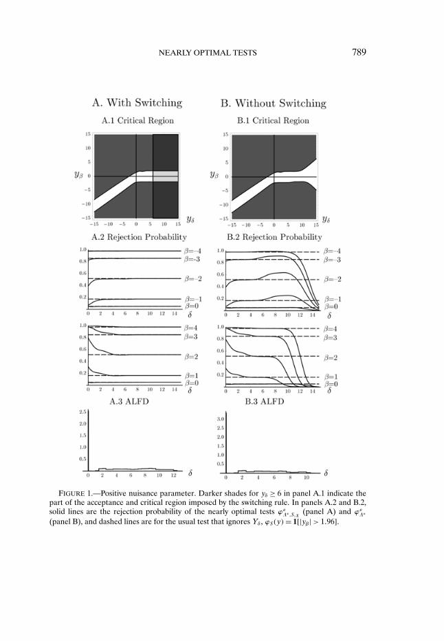
RUNNING EXAMPLE—ctd: We choose κδ = 9, so that Θ1�N consists of pa-rameter values θ = (β�δ) with β �= 0 and 0 ≤ δ ≤ 9. The weighting function Fis such that δ is uniformly distributed on [0�9], and β takes on the values −2and 2 with equal probability. The two alternatives are thus treated symmetri-cally and the values ±2 are chosen so that the test achieves approximately 50%power (following the rationale given in King (1987)). The switching function isspecified as χ(y)= 1[δ > 6], where δ= yδ.

Figure 1 summarizes the results for the running example with ρ = 0�7 fortests of level α = 5%. The ALFD was computed using ε = 0�005, so that thepower of the nearly optimal tests differs from the power bound by less than0�5 percentage points. The number of Monte Carlo draws under the null andalternative hypotheses in the algorithm are chosen so that Monte Carlo stan-dard errors are approximately 0.1%. Panel A shows results for ϕε

Λ∗�S�χ, and forcomparison, panel B shows results for the WAP maximizing test with the sameweighting function F with support on Θ1�N , but without the constraint to theswitching form (16).

The white and light gray band in the center of panel A.1 is the acceptanceregion of the nearly optimal test ϕε

Λ∗�S�χ, with the light gray indicating the ac-ceptance region conditional on switching (|yβ| ≤ 1�96 and yδ ≥ 6). The darkshades show the critical region, with the darker shade indicating the criticalregion conditional on switching (|yβ| > 1�96 and yδ ≥ 6). The critical region isseen to evolve smoothly as the test switches at yδ = 6, and essentially coincideswith the standard test ϕS for values of yδ as small as yδ = 3. This suggests thatother choices of κδ and κχ (and corresponding F with δ uniform on [0�κδ])would yield similar WAP maximizing tests; unreported results show that this isindeed the case. As yδ becomes negative, the critical region is approximately|yβ − ρyδ| > 1�96

√1 − ρ2, which is recognized as the critical region of the uni-

formly best unbiased test for δ= 0 known.Panel A.2 shows power (plotted as a function of δ) for selected values of β.

The solid curves show the power of the nearly optimal test and the dashed

8A necessary condition for tests of the form (16) to control size is that the “pure switching test”ϕ = χϕS (i.e., (16) with ϕN = 0) is of level α. Depending on the problem and choice of κχ, thismight require a slight modification of the most natural choice for ϕS to ensure actual (and notjust approximate) size control of ϕS for all δ > κδ.


FIGURE 1.—Positive nuisance parameter. Darker shades for yδ ≥ 6 in panel A.1 indicate thepart of the acceptance and critical region imposed by the switching rule. In panels A.2 and B.2,solid lines are the rejection probability of the nearly optimal tests ϕε

Λ∗�S�χ (panel A) and ϕεΛ∗

(panel B), and dashed lines are for the usual test that ignores Yδ, ϕS(y)= 1[|yβ| > 1�96].


lines show the power of the standard test ϕS . The figures show that power isasymmetric in β, with substantially lower power for negative values of β whenδ is small; this is consistent with the critical region shown in panel A.1 wherenegative values of β and small values of δ make it more likely that y fallsin the lower left quadrant of panel A.1. Because weighted average power iscomputed for uniformly distributed β ∈ {−2�2} and δ ∈ [0�9], the optimal testmaximizes the average of the power curves for β = −2 and β = 2 in panel A.2over δ ∈ [0�9]. Weighted average power of ϕε

Λ∗�S�χ is higher than the power ofϕS for all pairs of values for β shown in the figure.

Panels B show corresponding results for the nearly optimal test ϕεΛ∗ that

does not impose switching to a standard test, computed using the algorithmas described in Section 3. Because F only places weight on values of δ that areless than 9, this test sacrifices power for values of δ > 9 to achieve more powerfor values of δ ≤ 9. The differences between the power function for ϕε

Λ∗�S�χ(shown in panel A) and ϕε

Λ∗ (shown in panel B) highlight the attractivenessof switching to a standard test: it allows F to be chosen to yield high averagepower in the nonstandard portion of the parameter space (small values of δ)while maintaining good power properties in other regions.

Panels A.3 and B.3 show the ALFDs underlying the two tests, which are mix-tures of uniform baseline densities fi used in the calculations. We emphasizethat the ALFDs are not direct approximations to the least favorable distri-butions, but rather are distributions that produce tests with nearly maximalweighted average power.

4.3. Power Bounds Under Additional Constraints on Power

The test ϕεΛ∗�S�χ (nearly) coincides with ϕS when θ ∈ Θ1�S , and thus is (nearly)

as powerful as the standard best test ϕlimS in the limiting problem in that part

of the parameter space; moreover, ϕεΛ∗�S�χ comes close to maximizing WAP on

Θ1�N among all tests of the form (16). A natural question is whether this class isrestrictive, in the sense that there exist tests outside this class that have betterWAP on Θ1�N . We investigate this in this section by computing a WAP upperbound for any test that satisfies the level constraint and achieves prespecifiedpower on Θ1�S .

To begin, decompose the alternative into two hypotheses corresponding toΘ1�N and Θ1�S :

H1�N :θ ∈Θ1�N and H1�S :θ ∈ Θ1�S�

Let πS(θ) = ∫χϕSfθ dv denote the rejection frequency for the test ϕ = χϕS ,

where, as above, χ is the switching function and ϕS is the standard test. Thetest ϕ is a useful benchmark for the performance of any test on Θ1�S , since it isa feasible level α test of H0 against H1 with power πS(θ) under H1�S that is veryclose to the power of the standard test ϕS , which in turn has power close to the


admissible test ϕlimS in the limiting problem. Now, consider tests that (a) are

of level α under H0, (b) maximize WAP under H1�N relative to the weightingfunction F in (8), and (c) achieve power of at least πS(θ) under H1�S .9 Using anargument similar to that underlying Lemma 1, a bound on the power of levelα tests of H0 against H1�F (cf. (8)) with power of at least πS(θ) for θ ∈ Θ1�S

can be constructed by considering tests that replace the composite hypothesesH0 and H1�S with simple hypotheses involving mixtures. Thus, let Λ0 denotea distribution for θ with support in Θ0 and let Λ1 denote a distribution withsupport in Θ1�S , and consider the simple hypotheses

H0�Λ0 :Y has density f0�Λ0 =∫

fθ dΛ0(θ)�

H1�Λ1 :Y has density f1�Λ1 =∫

fθ dΛ1(θ)�

Let πS = ∫πS(θ)dΛ1(θ) denote the weighted average of the power bound un-

der H1�S . The form of the best tests for these simple hypotheses is described bya generalized Neyman–Pearson Lemma.

LEMMA 3: Suppose there exist cv0 ≥ 0, cv1 ≥ 0, and 0 ≤ κ ≤ 1 such that the test

ϕNP =⎧⎨⎩

1 if g + cv1 f1�Λ1 > cv0 f0�Λ0 ,κ if g + cv1 f1�Λ1 = cv0 f0�Λ0 ,0 if g + cv1 f1�Λ1 < cv0 f0�Λ0 ,

satisfies∫ϕNPf0�Λ0 dν = α,

∫ϕNPf1�Λ1 dν ≥ πS , and cv1(

∫ϕNPf1�Λ1 dν − πS)= 0.

Then for any other test satisfying∫ϕf0�Λ0 dν ≤ α and

∫ϕf1�Λ1 dν ≥ πS ,∫

ϕNPgdν ≥ ∫ϕgdν.

PROOF: If cv1 = 0, the result follows from the Neyman–Pearson Lemma. Forcv1 > 0, by the definition of ϕNP,

∫(ϕNP −ϕ)(g+ cv1 f1�Λ1 − cv0 f0�Λ0)dν ≥ 0. By

assumption,∫(ϕNP −ϕ)f1�Λ1 dν ≤ 0 and

∫(ϕNP −ϕ)f0�Λ0 dν ≥ 0. The result now

follows from cv0 ≥ 0 and cv1 ≥ 0. Q.E.D.

As in Lemma 1, the power of the Neyman–Pearson test for the simple hy-potheses provides an upper bound on power against H1�F when H0 and H1�S

are composite.

LEMMA 4: Let ϕNP denote the Neyman–Pearson test defined in Lemma 3,and let ϕ denote any test that satisfies (a) supθ∈Θ0

∫ϕfθ dν ≤ α and

(b) infθ∈Θ1�S [∫ϕfθ dν −πS(θ)] ≥ 0. Then

∫ϕNPgdν ≥ ∫

ϕgdν.

9This is an example in the class of constraints considered by Moreira and Moreira (2013).


PROOF: Because∫ϕf0�Λ0 dν ≤ α and

∫ϕf1�Λ1 dν ≥ ∫

πS(θ)dΛ1(θ) = πS , theresult follows from Lemma 3. Q.E.D.

Of course, to be a useful guide for gauging the efficiency of any proposedtest, the power bound should be as small as possible. For given α and powerfunction πS(θ) of ϕ = ϕSχ, the numerical algorithm from the last section canbe modified to compute distributions Λ∗

0 and Λ∗1 that approximately minimize

the power bound. Details are provided in Appendix A. We use this algorithmto assess the efficiency of the level α switching test ϕε

Λ∗�S�χ, which satisfies thepower constraint of Lemma 4 by construction, as ϕε

Λ∗�S�χ(y)≥ ϕ(y) for all y .

RUNNING EXAMPLE—ctd: The power bound from Lemma 4 evaluated atΛ∗

0 and Λ∗1 is 53.5%. Thus, there does not exist 5% level test with WAP larger

than 53.5% and with at least as much power as the test ϕ(y) = χ(y)ϕS(y) =1[δ > 6]1[|yβ| > 1�96] for alternatives with δ ≥ 9. Since ϕΛ∗�S�χ of panel A ofFigure 1 is strictly more powerful than ϕ, and it has WAP of 53.1%, it is thusalso nearly optimal in the class of 5% level tests that satisfy this power con-straint.

5. APPLICATIONS

In this section, we apply the algorithm outlined above (with the same param-eters as in the running example) to construct nearly weighted average powermaximizing 5% level tests for five nonstandard problems. In all of these prob-lems, we set ε = 0�005, so that the ALFD test has power within 0.5% of thepower bound for tests of the switching rule form (16) (if applicable). Unre-ported results show that the weighted average power of the resulting tests isalso within 0.0065 of the upper bound on tests of arbitrary functional formunder the power constraint described in Section 4.3 above.10 Appendix B ofthe Supplemental Material (Elliott, Müller, and Watson (2015)) contains fur-ther details on the computations in each of the problems, and Appendix C ofthe Supplemental Material contains tables and Matlab programs to implementthese nearly optimal tests for a wide range of parameter values.

5.1. The Behrens–Fisher Problem

Suppose we observe i.i.d. samples from two normal populations x1�i ∼N (μ1�σ

21 ), i = 1� � � � � n1 and x2�i ∼ N (μ2�σ

22 ), i = 1� � � � � n2, where n1� n2 ≥ 2.

We are interested in testing H0 :μ1 = μ2 without knowledge of σ21 and σ2

2 . Thisis the “Behrens–Fisher” problem, which has a long history in statistics. It also

10In some of these examples, we restrict attention to tests that satisfy a scale or location invari-ance property. Our ALFD test then comes close to maximizing weighted average power amongall invariant tests.


arises as an asymptotic problem when comparing parameters across two po-tentially heterogeneous populations, where the information about each popu-lation is in the form of n1 and n2 homogeneous clusters to which a central limittheorem can be applied (see Ibragimov and Müller (2010, 2013)).

Let xj = n−1j

∑nji=1 xj�i and s2

j = 1nj−1

∑nji=1(xj�i − xj)

2 be the sample means andvariances for the two groups j = 1�2, respectively. It is readily seen that thefour-dimensional statistic (x1� x2� s1� s2) is sufficient for the four parameters(μ1�μ2�σ1�σ2). Imposing invariance to the transformations (x1� x2� s1� s2) →(cx1 + m�cx2 + m�cs1� cs2) for m ∈ R and c > 0 further reduces the problemto the two-dimensional maximal invariant Y

Y = (Yβ�Yδ)=(

x1 − x2√s2

1/n1 + s22/n2

� log(s1

s2

))

whose density is derived in Appendix B of the Supplemental Material (cf.Linnik (1966) and Tsui and Weerahandi (1989)). Note that Yβ is the usualtwo-sample t-statistic which converges to N (0�1) under the null hypothesisas n1� n2 → ∞. The distribution of Y only depends on the two parametersβ = (μ1 −μ2)/

√σ2

1/n1 + σ22/n2 and δ = log(σ1/σ2), and the hypothesis prob-

lem becomes

H0 :β= 0� δ ∈ R against H1 :β �= 0� δ ∈ R�(17)

While the well-known two-sided test of Welch (1947) with “data-dependentdegrees of freedom” approximately controls size for sample sizes as small asmin(n1� n2) = 5 (Wang (1971) and Lee and Gurland (1975)), it is substan-tially oversized when min(n1� n2) ≤ 3; moreover, its efficiency properties areunknown. Thus, we employ the algorithm described above to compute nearlyoptimal tests for n1 ∈ {2�3} and n1 ≤ n2 ≤ 12; these are described in detailin the Supplemental Material. In the following, we focus on the two cases(n1� n2) ∈ {(3�3)� (3�6)}.

To implement the algorithm, we choose F as uniform on δ ∈ [−9�9] andβ = {−3�3}. Appendix A shows that as |δ| → ∞, the experiment converges toa one sample normal mean problem (since one of the samples has negligiblevariance).11 In the limiting problem, the standard test is simply the one samplet-test with n1 − 1 or n2 − 1 degrees of freedom, depending on the sign of δ.Thus, ϕS(y)= 1[yδ > 0]1[|yβ|> Tn1−1(0�975)]+1[yδ < 0]1[|yβ| > Tn2−1(0�975)],where Tn(x) is the xth quantile of a Student-t distribution with n degrees offreedom. We use the switching function χ(y) = 1[|yδ| > 6]. We compare thepower of the resulting ϕε

Λ∗�S�χ test to the “conservative” test obtained by usingthe 0�975 quantile of a Student-t distribution with degrees of freedom equal tomin(n1� n2)− 1, which is known be of level α (cf. Mickey and Brown (1966)).

11Strictly speaking, there are two limit experiments, one as δ→ ∞, and one as δ → −∞.


FIGURE 2.—Behrens–Fisher problem. Darker shades for |yδ| ≥ 6 in panels A.1 and B.1 indi-cate the part of the acceptance and critical region imposed by the switching rule. In panels A.2and B.2, solid lines are the rejection probability of the nearly optimal test ϕε

Λ∗�S�χ, and dashedlines are for the usual t-test with critical value computed from the Student-t distribution withn1 − 1 degrees of freedom.

Results are shown in Figure 2, where panel A shows results for (n1� n2) =(3�3) and panel B shows results for (n1� n2) = (3�6). Looking first at panel A,the critical region transitions smoothly across the switching boundary. In thenonstandard part (|yδ|< 6), the critical region is much like the critical region ofthe standard test 1[|yβ|> T2(0�975)] for values of |yδ|> 2, but includes smallervalues of |yβ| when yδ is close to zero. Evidently, small values of |yδ| suggest thatthe values of σ1 and σ2 are close, essentially yielding more degrees of freedom


for the null distribution of yβ. This feature of the critical region translates inthe greater power for ϕε

Λ∗�S�χ than the conservative test when δ is close to zero(see panel A.2). Panel B shows results when n2 is increased to n2 = 6. Now,the critical region becomes “pinched” around yδ ≈ −1 apparently capturing atrade-off between a relatively small value of s1 and n1. Panel B.2 shows a powerfunction that is asymmetric in δ, where the test has more power when the largergroup has larger variance. Finally, the conservative test has a null rejectionfrequency substantially less than 5% when δ < 0 and weighted average powersubstantially below the nearly optimal test.

5.2. Inference About the Break Date in a Time Series Model

In this section, we consider tests for the break date τ in the parameter of atime series model with T observations. A leading example is a one-time shift bythe amount η of the value of a regression coefficient, as studied in Bai (1994,1997). Bai’s asymptotic analysis focuses on breaks that are large relative tosampling uncertainty by imposing T 1/2|η| → ∞. As discussed in Elliott andMüller (2007), this “large break” assumption may lead to unreliable inferencein empirically relevant situations.

Under an alternative embedding for moderately sized breaks T 1/2η→ δ ∈ R,the parameter δ becomes a nuisance parameter that remains relevant evenasymptotically. As a motivating example, suppose the mean of a Gaussian timeseries shifts at some date τ by the amount η,

yt = μ+ 1[t ≥ τ]η+ εt� εt ∼ i.i.d. N (0�1)�

and the aim is to conduct inference about the break date τ. As is standard in thestructural break literature, assume that the break does not happen close to thebeginning and end of the sample, that is, with β = τ/T , β ∈ B = [0�15�0�85].Restricting attention to translation invariant tests ({yt} → {yt + m} for all m)requires that tests are a function of the demeaned data yt − y . Partial summingthe observations yields

T−1/2�sT �∑t=1

(yt − y)∼G(s) = W (s)− sW (1)− δ(min(β� s)−βs

)(18)

for s = j/T and integer 1 ≤ j ≤ T , where W is a standard Wiener process. Thissuggests that asymptotically, the testing problem concerns the observation ofthe Gaussian process G on the unit interval, and the hypothesis of interest con-cerns the location β of the kink in its mean. Elliott and Müller (2014) formallyshowed that this is indeed the relevant asymptotic experiment for a moder-ate structural break in a well-behaved parametric time series model. By Gir-


sanov’s Theorem, the Radon–Nikodym derivative of the measure of G in (18)relative to the measure ν of the standard Brownian Bridge, evaluated at G, isgiven by

fθ(G)= exp[−δG(β)− 1

2δ2β(1 −β)

]�(19)

For |δ| > 20, the discretization of the break date β becomes an importantfactor in this limiting problem, even with 1000 step approximations to Wienerprocesses. Since these discretization errors are likely to dominate the analysiswith typical sample sizes for even larger δ, we restrict attention to δ ∈ Δ =[−20�20], so that the hypotheses are

H0 :β= β0� δ ∈ Δ against H1 :β �= β0� δ ∈ Δ�

To construct the ALFD test, we choose F so that β is uniform on B and δ isN (0�100), truncated to Δ. Results are shown in Figure 3. Panel A shows resultsfor β0 = 0�2, where panel A.1 plots power as a function of β for five values of δ;panel B shows analogous results for β0 = 0�4. (Since G is a continuous timestochastic process, the sample space is of infinite dimension, so it is not possible

FIGURE 3.—Break date. In panels A.1 and B.1, solid lines are the rejection probability of thenearly optimal test ϕε

Λ∗ , and dashed lines are for Elliott and Müller’s (2007) test that imposes anadditional invariance.


to plot the critical region.) Rejection probabilities for a break at β0 > 0�5 areidentical to those at 1 −β0.

Also shown in the figures are the corresponding power functions from thetest derived in Elliott and Müller (2007) that imposes the additional invariance

G(s)→ G(s)+ c(min(β0� s)−β0s

)for all c�(20)

This invariance requirement eliminates the nuisance parameter δ under thenull, and thus leads to a similar test. But the transformation (20) is not naturalunder the alternative, leaving scope for reasonable and more powerful teststhat are not invariant. Inspection of Figure 3 shows that the nearly optimal testϕε

Λ∗ has indeed substantially larger power for most alternatives. Also, power isseen to be small when β is close to either β0 or the endpoints, as this implies amean function close to what is specified under the null hypothesis.

5.3. Predictive Regression With a Local-to-Unity Regressor

A number of macroeconomic and finance applications concern the coeffi-cient γ on a highly persistent regressor xt in the model

yt = μ+ γxt−1 + εy�t�(21)

xt = rxt−1 + εx�t� x0 = 0�

where E(εy�t |{εx�t−j}t−1j=1) = 0, so that the first equation is a predictive regres-

sion. The persistence in xt is often modeled as a local-to-unity process (in thesense of Bobkoski (1983), Cavanagh (1985), Chan and Wei (1987), and Phillips(1987)) with r = rT = 1 −δ/T . Interest focuses on a particular value of γ givenby H0 :γ = γ0 (where typically γ0 = 0). When the long-run covariance betweenεy and εx is nonzero, the usual t-test on γ is known to severely overreject unlessδ is very large.

After imposing invariance to translations of yt , {yt} → {yt + m}, and an ap-propriate scaling by the (long-run) covariance matrix of (εy�t� εx�t)

′, the asymp-totic inference problem concerns the likelihood ratio process fθ of a bivariateGaussian continuous time process G,

fθ(G)= K(G)exp[βY1 − δY2 − 1

2

(β+ ρ√

1 − ρ2δ

)2

Y3 − 12δ2Y4

]�(22)

where β is proportional to T(γ − γ0), ρ ∈ (−1�1) is the known (long-run)correlation between εx�t and εy�t , θ = (β�δ)′ ∈ R

2 is unknown, and the four-dimensional sufficient statistic Y = (Y1�Y2�Y3�Y4) has distribution

Y1 =∫ 1

0W μ

x�δ(s)dWy(s)+(β+ ρ√

1 − ρ2δ

)∫ 1

0W μ

x�δ(s)2 ds�


Y2 =∫ 1

0Wx�δ(s)dWx�δ(s)− ρ√

1 − ρ2Y1�

Y3 =∫ 1

0W μ

x�δ(s)2 ds� Y4 =

∫ 1

0Wx�δ(s)

2 ds�

where Wx and Wy are independent standard Wiener processes, and theOrnstein–Uhlenbeck process Wx�δ solves dWx�δ(s) = −δWx�δ(s)ds + dWx(s)

with Wx�δ(0) = 0, and W μx�δ(s) = Wx�δ(s) − ∫ 1

0 Wx�δ(t)dt (cf. Jansson and Mor-eira (2006)).

Ruling out explosive roots, δ < 0, the one-sided asymptotic inference prob-lem is

H0 :β= 0� δ ≥ 0 against H1 :β> 0� δ ≥ 0�(23)

While several methods have been developed that control size in (23) (lead-ing examples include Cavanagh, Elliott, and Stock (1995) and Campbell andYogo (2006)), there are fewer methods with demonstrable optimality. Stockand Watson (1996) numerically determined a weighted average power maxi-mizing test within a parametric class of functions R4 �→ {0�1}, and Jansson andMoreira (2006) derived the best conditionally unbiased tests of (23), condi-tional on the specific ancillary (Y3�Y4). However, Jansson and Moreira (2006)reported that Campbell and Yogo’s (2006) test has higher power for most alter-natives. We therefore compare the one-sided ALFD test to this more powerfulbenchmark.

In Appendix A, we show that in a parameterization with δ= Δn−d√

2Δn andβ = b

√2Δn/(1 − ρ2), the experiment of observing G converges as Δn → ∞ to

the unrestricted two-dimensional Gaussian shift experiment. A natural way toobtain a test with the same asymptotic power function as δ → ∞ is to rely onthe usual maximum likelihood t-test (with observed information). From (22),the MLE is given by

β= Y1

Y3− ρ√

1 − ρ2δ� δ= −

Y2 + ρ√1 − ρ2

Y1

Y4�

and the standard test becomes ϕS(Y) = 1[β/√Y−1

3 + ρ2

1−ρ2 Y−14 > cvS].

For numerical convenience, we use a discrete weighting function F withequal mass on 51 pairs of values (β�δ), where δ ∈ {0�0�252�0�52� � � � �12�52}and the corresponding values for β equal

β= b

√2δ+ 61 − ρ2 for δ > 0(24)


FIGURE 4.—Predictive regression with a local-to-unity regressor. In panels A.1 and B.1, solidlines are the rejection probability of the nearly optimal test ϕε

Λ∗�S�χ, and dashed lines are forCampbell and Yogo’s (2006) test. Since the latter is constructed under the assumption that δ ≤ 50,we only report its rejection probability for δ ∈ [0�40]. Alternatives are parameterized as in (24),with b ∈ {0�1�2�3�4}.

for b = 1�645. These alternatives are chosen so that power against each pointin F is roughly 50%. (The spacing of the mass points for δ and the choice ofβ correspond to an approximately uniform weighting over d and an alterna-tive of 1�645 standard deviations for b in the limiting experiment.) We use theswitching function χ(Y) = 1[δ ≥ 130]. The critical value cvS in ϕS equals theusual 5% level value of 1.645 when ρ≥ 0, but we choose cvS = 1�70 when ρ < 0.This slight adjustment compensates for the heavier tail of the t-test statistic formoderate values of δ and negative ρ.

Figure 4 compares the power of the resulting nearly optimal test to the testdeveloped by Campbell and Yogo (2006) under the practically relevant valuesof ρ= −0�5 and ρ= −0�9. Because the Campbell and Yogo (2006) test utilizesa confidence set for r with correct coverage only when r is close to unity (seeMikusheva (2007) and Phillips (2014)), Figure 4 plots power for δ in the re-stricted range 0 ≤ δ≤ 40, and over this range the optimal test nearly uniformlydominates the alternative test. For values of δ > 40 (so that r is much lessthan unity), the power of the Campbell and Yogo (2006) test falls dramatically,while the power of the optimal test increases slightly from its value with δ= 40,and smoothly transitions to the power of ϕS . Unreported results show similar


results for positive values of ρ. In the Supplemental Material Appendix B, wealso provide a comparison of our test with a modification of the Campbell andYogo (2006) procedure that inverts Hansen’s (1999) confidence intervals for r,which does not suffer from the uniformity issues mentioned above, and againfind that our test dominates in terms of power.

5.4. Testing the Value of a Set-Identified Parameter

The asymptotic problem introduced by Imbens and Manski (2004) and fur-ther studied by Woutersen (2006), Stoye (2009), and Hahn and Ridder (2011)involves a bivariate observation

Y =(Yl

Yu

)∼N

((μl

μu

)�

(σ2

l ρσlσu

ρσlσu σ2u

))�

where μl ≤ μu, and the elements σl�σu > 0 and ρ ∈ (−1�1) of the covariancematrix are known. The object of interest is μ, which is only known to satisfy

μl ≤ μ ≤ μu�(25)

Without loss of generality, suppose we are interested in testing H0 :μ = 0 (thetest of the general hypothesis μ = μ0 is reduced to this case by subtracting μ0

from Yl and Yu). Whilst under the null hypothesis the inequality (25) holdsif and only if μl/σl ≤ 0 ≤ μu/σu, under the alternative the normalized meansμl/σl and μu/σu may no longer satisfy the ordering μl/σl ≤ μu/σu. It is thusnot possible to reduce this problem to a single known nuisance parameter ρwithout loss of generality. In the sequel, we demonstrate our approach whenσl = σu = 1 and various values of ρ.

It is useful to reparameterize (μl�μu) in terms of (β�δL�δP) ∈ R3 as follows:

let δL = μu −μl be the length of the identified set [μl�μu], let β= μl if μl > 0,β= μu if μu < 0, and β= 0 otherwise, and let δP = −μl, so that under the nullhypothesis δP describes the position of 0 in the identified set. In this parame-terization, the hypothesis testing problem becomes

H0 :β= 0� δL ≥ 0� δP ∈ [0� δL] against H1 :β �= 0� δL ≥ 0�(26)

Appendix A shows that the limiting problem as δL → ∞ becomes a sim-ple one-sided testing problem in the Gaussian shift experiment (2) with un-restricted nuisance parameter space. Thus, in this limiting problem, the stan-dard test can be written as ϕS(y) = 1[yl > 1�645 or yu < −1�645]. We switchto this standard test according to χ(y) = 1[δL > 6], where δL = Yu − Yl ∼N (δL�2(1 − ρ)). The weighting function F is chosen to be uniform on δL ∈[0�9], with equal mass on the two points β ∈ {−2�2}.

Note that (26) has a two-dimensional nuisance parameter under the null hy-pothesis, as neither the length δL = μu − μl nor the distance δP of μl from


zero is specified under H0. It is reasonable to guess, though, that the least fa-vorable distribution only has mass at δP ∈ {0� δL}, so that one of the endpointsof the interval coincides with the hypothesized value of μ. Further, the prob-lem is symmetric in these two values for δP . In the computation of the ALFD,we thus impose δP ∈ {0� δL} with equal probability, and then check that theresulting test ϕε

Λ∗�S�χ does indeed control size also for δP ∈ (0� δL).Figure 5 shows results for two values of ρ. Looking first at the critical re-

gions, when yu is sufficiently large (say yu > 2), the test rejects when yl > 1�645,

FIGURE 5.—Set-identified parameter. Darker shades for yu + yl ≥ 6 in panels A.1 and B1indicate the part of the acceptance and critical region imposed by the switching rule. In panels A.2and B.2, solid lines are the rejection probability of the nearly optimal tests ϕε

Λ∗�S�χ, and dashedlines are for Stoye’s (2009) test ϕStoye(y)= 1[yl > 1�96 or yu <−1�96].


and similarly when yl is sufficiently negative. The upper left-hand quadrant ofthe figures in panels A.1 and B.1 shows the behavior of the test when the obser-vations are inverted relative to their mean values, yl > yu. In that case, the testrejects unless yl + yu is close to zero. Panels A.2 and B.2 compare the power ofthe ALFD test ϕε

Λ∗�S�χ to the test ϕStoye(y)= 1[yl > 1�96 or yu < −1�96], which islarge sample equivalent to Stoye’s (2009) suggestion under local asymptotics.Note that this test has null rejection probability equal to 5% when δL = 0 andδP ∈ {0� δL}. Not surprisingly, ϕε

Λ∗�S�χ dominates ϕStoye when δL is large, but italso has higher power when δL is small and ρ= 0�5 (because when δL is small,the mean of Yl and Yu is more informative about μ than either Yl or Yu unlessρ is close to 1).

5.5. Regressor Selection

As in Leeb and Pötscher (2005), consider the bivariate linear regression

yi = γxi +ηzi + εi� i = 1� � � � � n�εi ∼N(0�σ2

)�(27)

where σ2 is known. We are interested in testing H0 :γ = γ0, and η is a nui-sance parameter. Suppose there is substantial uncertainty whether the addi-tional control zi needs to be included in (27), that is, η = 0 is deemed likely,but not certain. Denote by (γ� η) the OLS estimators from the “long” regres-sion of yi on (xi� zi). Let β= n1/2(γ−γ0), δ= n1/2η, (Yβ�Yδ)= n1/2(γ−γ0� η),and for notational simplicity, assume that the regressors and σ2 have been scalenormalized so that

Y =(Yβ

Yδ

)∼N

((βδ

)�

(1 ρρ 1

))�(28)

where −ρ is the known sample correlation between xi and zi. Note that withthe Gaussian assumption about εi, Y is a sufficient statistic for the unknownparameters (β�δ).

For δ= 0 known, the statistic Yβ −ρYδ is more informative about β than Yβ.Intuitively, Yβ − ρYδ is the (rescaled) regression coefficient in the “short” re-gression of yi on xi, omitting zi, while Yβ corresponds to the coefficient in the“long” regression. Ideally, one would like to let the data decide whether indeedδ = 0, so that one can appropriately base inference on Yβ − ρYδ, or on Yβ. Asreviewed by Leeb and Pötscher (2005), however, data-dependent model selec-tion procedures do not perform uniformly well for all values of η, even in largesamples, so that optimal inference is not obtained in this manner.

As one possible notion of optimality, suppose that we seek a test of H0 :β= 0that is as powerful as possible when δ= 0, but under the constraint that the testcontrols size for all values of δ ∈ R. The idea is that we want to maximize powerin the a priori likely case of δ = 0, while at the same time controlling the nullrejection probability even if δ �= 0.


Consider first the one-sided problem. With F degenerate at β1 > 0, we ob-tain the hypothesis test

H0 :β= 0� δ ∈ R against H1�F :β= β1� δ = 0�(29)

Note that rejecting for large values of Yβ is the Neyman–Pearson test of H1�F

against the single null hypothesis Hs0 : (β�δ) = (0� δ0), where δ0 = −ρβ1. Since

any level α test of (29) is also of level α under Hs0, the uniformly most powerful

one-sided test of (29) thus rejects for large values of Yβ (cf. Proposition 15.2in van der Vaart (1998)). Thus, as long as one insists on uniform size control,the question of best one-sided inference about β has a straightforward answer:simply rely on the coefficient estimate of the long regression.

Now consider the two-sided problem. It is known that rejecting for largevalues of |Yβ| yields the uniformly most powerful test among tests that areunbiased for all values of δ ∈ R (cf. problem 1 on page 226 of van der Vaart(1998)). But with a focus on power at the point δ= 0, this might be considereda too restrictive class of tests. Thus, we consider the unconstrained problem ofmaximizing weighted average power in the hypothesis testing problem

H0 :β= 0� δ ∈ R against H1 :β �= 0� δ = 0(30)

and choose a weighting function F that puts equal mass at the two points{−2�2}. For large |Yδ|, we switch to the standard test ϕS(y) = 1[|yβ| > 1�96]via χ(y) = 1[|yδ| > 6]. Unreported results show that imposing this switchingrule leads to no discernible loss in power when δ = 0. At the same time, thisswitching rule leads to much higher power when |δ| is large.

By construction, the weighted average power at δ = 0 of ϕεΛ∗�S�χ in Figure 6

is nearly the largest possible among all 5% valid tests. To get a more compre-hensive view of the potential gains in power as a function of ρ, Figure 7 depictsthe power bound, the power of ϕε

Λ∗�S�χ, and the power of ϕS against δ = 0 andβ ∈ {−2�2}. The experiment (28) becomes more informative about β as ρ in-creases, and correspondingly, the power bound is an increasing function of ρ.12

It is striking, though, how flat the power bound becomes once ρ ≥ 0�75. Thegains in power at δ = 0 over the standard test ϕS are never larger than 12percentage points, and the test ϕε

Λ∗�S�χ described in the Supplemental Materialcomes very close to fully exploiting the available information.

6. CONCLUSION

Many statistics have been explored as the basis for constructing valid testsin nonstandard econometric problems: maximum likelihood estimators, quasi

12Adding mean-zero Gaussian noise to Yδ and an appropriate rescaling yields an equivalentexperiment with smaller |ρ|.


FIGURE 6.—Regressor selection. Darker shade for |yδ| ≥ 6 in panels A.1 and B.1 is the partof the critical region imposed by the switching rule. In panels A.2 and B.2, solid lines are therejection probability of the nearly optimal tests ϕε

Λ∗�S�χ, and dashed lines are for the usual testthat ignores Yδ, ϕS(y) = 1[|yβ| > 1�96].

likelihood ratio statistics, moment based criterion functions, statistics involvingpretests, etc. Similarly, appropriate critical values may be obtained by variousmethods: by searching for the largest appropriate quantile of the test statisticunder the null hypothesis, by arguing for the validity of bootstrap or subsam-


FIGURE 7.—Weighted average power in regressor selection problem as function of ρ. Thicksolid line is power bound, thin solid line is power of 5% level test, and dashed line is power ofusual test that ignores Yδ, ϕS(y)= 1[|yβ| > 1�96].

pling methods, or by refining these approaches with Bonferroni inequalities orpretests.

The numerical determination of an approximately least favorable null distri-bution suggested here is, in general, not substantially harder, either conceptu-ally or computationally. And, in contrast to these other approaches, it deliversa test that is nearly optimal in the sense that it comes close to maximizing aweighted average power criterion. What is more, once the approximate leastfavorable distribution is determined, the test is straightforward to implementin practice, compared to, say, methods that require resampling. Also, the lowupper bound on weighted average power implied by the approximately leastfavorable distribution can be used to argue for the near-optimality of a conve-nient test statistic, such as the quasi likelihood ratio statistic. For these reasons,the algorithm suggested here seems a practically useful approach to deal withnonstandard testing problems.

The six applications considered in this paper have a one-dimensional nui-sance parameter, and Müller and Watson (2013b) and Müller (2014) discussedadditional applications with a one-dimensional nuisance parameter. While ahigh-dimensional nuisance parameter generally poses numerical difficulties forthe algorithm, Müller and Watson (2013a) successfully implemented the algo-rithm in a problem with a three-dimensional nuisance parameter. The rela-tively hardest part in the computations is the numerical check of size control,but unless the problem has special features, the difficulty of this step is com-mon to all approaches to constructing nontrivial tests.

APPENDIX A

A.1. Proof of Lemma 2

For any h0, we have, from (11),

fn�h0(Y)

fn�0(Y)⇒ fX�h0(X)

fX�0(X)�


so that fn�h0 is contiguous to fn�0 by LeCam’s first lemma. A general versionof LeCam’s third lemma (see, for instance, van der Vaart (2002)) thus impliesthat (11) also holds with Y and X distributed according to fn�h0 and fX�h0 , re-spectively. This establishes convergence of experiments via Definition 9.1 ofvan der Vaart (1998).

With ε = lim supΔ→∞(E(b1�Δ)[ϕ(Y)] − E(b1�Δ)[ϕS(Y)]) > 0, pick Δn withΔn → ∞ such that limn→∞(E(b1�Δn)[ϕ(Y)] −E(b1�Δn)[ϕS(Y)])= ε. With this def-inition of Δn, E(b�Δn)[·] corresponds to integration w.r.t. fn�h, where h= (b�0) ∈R

kβ+1, denoted by En�h[·]. By assumption about ϕS and ϕlimS , En�h1[ϕS(Y)] →

Eh1[ϕlimS (X)], where h1 = (b1�0). Thus, En�h1[ϕ(Y)] → Eh1[ϕlim

S (X)] + ε. Fur-ther, by contiguity, also En�h[ϕ(Y)] converges for all fixed h. By Theo-rem 15.1 of van der Vaart (1998), there exists a test ϕlim with a power func-tion Eh[ϕlim(X)] equal to limn→∞ En�h[ϕ(Y)]. The test ϕlim is of level α, asE(0�δn)[ϕ(Y)] ≤ α for all n implies limn→∞ E(0�δn)[ϕ(Y)] ≤ α. Further, sinceϕlim

S is admissible with a power function that does not depend on d, andϕlim has higher power than ϕlim

S at b = b1, there must exist b2 such thatwith h2 = (b2�0), Eh2[ϕlim(X)] < Eh2[ϕlim

S (X)]. The conclusion follows fromEn�h2[ϕ(Y)] → Eh2[ϕlim(X)] and En�h2[ϕS(Y)] → Eh2[ϕlim

S (X)].

A.2. Algorithm Details

A.2.1. Details of the Algorithm Described in Section 3

Repeated application of (10) requires evaluation of the rejection probabil-ity

∫ϕμfj dν. This can be implemented straightforwardly by Monte Carlo in-

tegration, using N0 independent draws Yj�l from fj , l = 1� � � � �N0, for a to-tal of M · N0 independent draws. Thus, one simple estimator of

∫ϕμfj dν is

N−10

∑N0l=1 1[g(Yj�l) >

∑M

i=1 exp(μi)fi(Yj�l)]. Note that the M ·N0 scalar randomvariables g(Yi�l) and M2 · N0 variables fi(Yj�l) can be computed and storedonce, prior to any fixed point iteration. But with fi readily available, it makessense to improve the estimator of

∫ϕμfj dν via importance sampling, that is,

to use

RPj(μ) = (MN0)−1

M∑k=1

N0∑l=1

fj(Yk�l)

f (Yk�l)1

[g(Yk�l) >

M∑i=1

exp(μi)fi(Yk�l)

]�(31)

where f (y) = M−1∑M

j=1 fj(y). This has the advantage that with a finer dis-cretization of H0 (larger M), one may decrease N0 for the same level of MonteCarlo accuracy, as the draws from neighboring densities become relativelymore informative for the rejection probability under fj .

The ultimate algorithm consists of the following eight steps:1. For each k, k = 1� � � � �M , generate N0 draws Yk�l, l = 1� � � � �N0, with den-

sity fk. The draws Yk�l are independent across k and l.


2. Compute and store g(Yk�l), fj(Yk�l), and f (Yk�l), j�k = 1� � � � �M , l =1� � � � �N0.

3. Set μ(0) = (−2� � � � �−2) ∈RM .

4. Compute μ(i+1) from μ(i) via μ(i+1)j = μ(i)

j + ω(RPj(μ(i)) − α) and ω = 2,

and repeat this step O = 600 times. Denote the resulting element in the simplexby Λ∗ = (λ∗

1� � � � � λ∗M), where λ∗

j = exp(μ(O)j )/

∑M

k=1 exp(μ(O)k ).

5. Compute the number cv such that the test ϕΛ∗ is exactly of (MonteCarlo) level α when Y is drawn from the mixture

∑M

i=1 λ∗i fi, that is, solve∑M

j=1 λ∗j (RP

∗j (cv) − α) = 0, where RP

∗j (cv) is the Monte Carlo estimate (31)

of the rejection probability of the test 1[g > cv∑M

i=1 λ∗i fi] under fj .

6. Compute the (estimate of) the power bound π of ϕΛ∗ = 1[g >

cv∑M

i=1 λ∗i fi] via N−1

1

∑N1l=1 ϕΛ∗(Yl), where Yl are N1 i.i.d. draws of Y with den-

sity g.13

7. Compute the number cvε > cv such that the test ϕε

Λ∗ = 1[g >

cvε∑M

i=1 λ∗i fi] has (estimated) power π − ε, using the same estimator as in

Step 6.8. Check size control of ϕε

Λ∗ by evaluating its null rejection probabilities ona fine grid of H0, using estimates of null rejection probabilities of the form(31). If ϕε

Λ∗ is found to overreject, restart the algorithm at Step 1 with a finer

discretization of H0 (larger M). Otherwise, Λ∗ satisfies the definition of anε-ALFD, Λ∗ = Λ∗.

With N0 = 20,000 and N1 = 100,000 (so that Monte Carlo standard devia-tions of RPj(μ) are about 0�1%) and M = 50, the algorithm takes about oneminute on a modern PC, and it spends most of the time on Steps 2 and 8.

In some additional problems not discussed in this paper, we found thatthe iterations of Step 4 can be accelerated by introducing iteration-specificand adaptive step length factors ω(i)

j , so that Step 4 reads μ(i+1)j =

μ(i)j + ω(i)

j (RPj(μ(i)) − α), where ω(i+1)

j is made much smaller (say, ω(i+1)j =

0�5ω(i)j ) if the size control constraint switches sign in the last two iterations

(RPj(μ(i)) − α)(RPj(μ

(i−1)) − α) < 0, and ω(i+1)j increases slowly otherwise

(say, ω(i+1)j = 1�03ω(i)

j ).

A.2.2. Details of the Algorithm Used to Compute ε-ALFD Switching Tests

First note the following result that extends Lemma 1 to tests of the switchingform (16).

13It makes sense to choose N1 > N0, as the importance sampling in (31) leads to a relativelysmaller Monte Carlo standard error.


LEMMA 5: For given χ and ϕS , let SW be the set of tests of the form (16). LetϕΛ�S�χ ∈ SW be of size α under H0�Λ with ϕΛ of the Neyman–Pearson form

ϕΛ =

⎧⎪⎪⎪⎪⎪⎪⎨⎪⎪⎪⎪⎪⎪⎩

1 if g(y) > cv∫

fθ(y)dΛ(θ),

κ if g(y)= cv∫

fθ(y)dΛ(θ),

0 if g(y) < cv∫

fθ(y)dΛ(θ),

for some cv ≥ 0 and 0 ≤ κ ≤ 1. Then for any test ϕ ∈ SW that is of level α un-der H0,

∫ϕΛ�S�χg dν ≥ ∫

ϕgdν.

PROOF: Note that by construction,∫(ϕΛ�S�χ −ϕ)(g − cv

∫fθ dΛ(θ))dν ≥ 0.

Since ϕ is of level α under H0,∫ϕfθ dν ≤ α for all θ ∈ Θ0. Therefore,∫∫

ϕfθ dν dΛ(θ)= ∫ϕ(

∫fθ dΛ(θ))dν ≤ α, where the equality follows from Fu-

bini’s Theorem. Thus∫(ϕΛ�S�χ − ϕ)(

∫fθ dΛ(θ))dν ≥ 0, and the result fol-

lows. Q.E.D.

Given this result, the only change to the algorithm of Section A.2.1 is thereplacement of ϕΛ and ϕε

Λ by ϕΛ�S�χ and ϕεΛ�S�χ, respectively. Specifically, the

(estimated) rejection probability (31) now reads

RPj(μ) = (MN0)−1

M∑k=1

N0∑l=1

fj(Yk�l)

f (Yk�l)

(χ(Yk�l)ϕS(Yk�l)

+ (1 −χ(Yk�l)

)1

[g(Yk�l) >

M∑i=1

exp(μi)fi(Yk�l)

])�

and in Steps 6 and 7, π and π − ε are the (estimated) powers of the testsϕΛ�S�χ = χϕS + (1 − χ)1[g > cv

∑M

i=1 λifi] and ϕε

Λ�S�χ= χϕS + (1 − χ)1[g >

cvε∑M

i=1 λifi], respectively. Correspondingly, the size check in Step 8 also con-cerns ϕε

Λ�S�χ.

REFERENCES

ANDREWS, D. W. K. (2011): “Similar-on-the-Boundary Tests for Moment Inequalities Exist, butHave Poor Power,” Discussion Paper 1815, Cowles Foundation. [772]

ANDREWS, D. W. K., AND G. GUGGENBERGER (2010): “Asymptotic Size and a Problem WithSubsampling and With the M out of N Bootstrap,” Econometric Theory, 26, 426–468. [775]

ANDREWS, D. W. K., AND W. PLOBERGER (1994): “Optimal Tests When a Nuisance Parameter IsPresent Only Under the Alternative,” Econometrica, 62, 1383–1414. [777]

http://www.e-publications.org/srv/ecta/linkserver/setprefs?rfe_id=urn:sici%2F0012-9682%28201503%2983%3A2%3C771%3ANOTWAN%3E2.0.CO%3B2-N

http://www.e-publications.org/srv/ecta/linkserver/openurl?rft_dat=bib:2/Andrews10&rfe_id=urn:sici%2F0012-9682%28201503%2983%3A2%3C771%3ANOTWAN%3E2.0.CO%3B2-N





ANDREWS, D. W. K., M. J. MOREIRA, AND J. H. STOCK (2008): “Efficient Two-Sided Nonsim-ilar Invariant Tests in IV Regression With Weak Instruments,” Journal of Econometrics, 146,241–254. [773,779]

BAI, J. (1994): “Least Squares Estimation of a Shift in Linear Processes,” Journal of Time SeriesAnalysis, 15, 453–470. [774,795]

(1997): “Estimation of a Change Point in Multiple Regressions,” Review of Economicsand Statistics, 79, 551–563. [774,795]

BLACKWELL, D., AND M. A. GIRSHICK (1954): Theory of Games and Statistical Decisions. NewYork: Wiley. [774,780]

BOBKOSKI, M. J. (1983): “Hypothesis Testing in Nonstationary Time Series,” Ph.D. Thesis, De-partment of Statistics, University of Wisconsin. [797]

CAMPBELL, J. Y., AND M. YOGO (2006): “Efficient Tests of Stock Return Predictability,” Journalof Financial Economics, 81, 27–60. [774,798-800]

CAVANAGH, C. L. (1985): “Roots Local to Unity,” Working Paper, Harvard University. [797]CAVANAGH, C. L., G. ELLIOTT, AND J. H. STOCK (1995): “Inference in Models With Nearly Inte-

grated Regressors,” Econometric Theory, 11, 1131–1147. [784,798]CHAMBERLAIN, G. (2000): “Econometric Applications of Maximin Expected Utility,” Journal of

Applied Econometrics, 15, 625–644. [774,783](2007): “Decision Theory Applied to an Instrumental Variables Model,” Econometrica,

75 (3), 609–652. [786]CHAN, N. H., AND C. Z. WEI (1987): “Asymptotic Inference for Nearly Nonstationary AR(1)

Processes,” The Annals of Statistics, 15, 1050–1063. [797]CHIBURIS, R. C. (2009): “Approximately Most Powerful Tests for Moment Inequalities,” in

“Essays on Treatment Effects and Moment Inequalities,” Ph.D. Thesis, Department of Eco-nomics, Princeton University, Chapter 3. [774,783]

CHOI, A., W. J. HALL, AND A. SCHICK (1996): “Asymptotically Uniformly Most Powerful Tests inParametric and Semiparametric Models,” The Annals of Statistics, 24, 841–861. [772,776]

DUFOUR, J.-M., AND M. L. KING (1991): “Optimal Invariant Tests for the Autocorrelation Co-efficient in Linear Regressions With Stationary or Nonstationary AR(1) Errors,” Journal ofEconometrics, 47, 115–143. [772]

ELLIOTT, G., AND U. K. MÜLLER (2007): “Confidence Sets for the Date of a Single Break inLinear Time Series Regressions,” Journal of Econometrics, 141, 1196–1218. [774,795-797]

(2012): “Pre and Post Break Parameter Inference,” Working Paper, Princeton Univer-sity. [783]

(2014): “Pre and Post Break Parameter Inference,” Journal of Econometrics, 180,141–157. [795]

ELLIOTT, G., U. K. MÜLLER, AND M. W. WATSON (2015): “Supplement to ‘Nearly Optimal TestsWhen a Nuisance Parameter Is Present Under the Null Hypothesis’,” Econometrica Supple-mental Material, 83, http://dx.doi.org/10.3982/ECTA10535. [792]

ELLIOTT, G., T. J. ROTHENBERG, AND J. H. STOCK (1996): “Efficient Tests for an AutoregressiveUnit Root,” Econometrica, 64, 813–836. [772]

FACCHINEI, F., AND J.-S. PANG (2003): Finite-Dimensional Variational Inequalities and Comple-mentarity Problems, Vols. I and II. New York: Springer. [784]

FERGUSON, T. S. (1967): Mathematical Statistics—A Decision Theoretic Approach. New York: Aca-demic Press. [774,781]

HAHN, J., AND G. RIDDER (2011): “A Dual Approach to Confidence Intervals for Partially Iden-tified Parameters,” Working Paper, UCLA. [800]

HANSEN, B. E. (1999): “The Grid Bootstrap and the Autoregressive Model,” Review of Economicsand Statistics, 81, 594–607. [800]

HILLIER, G. (1990): “On the Normalization of Structural Equations: Properties of Direction Es-timators,” Econometrica, 58, 1181–1194. [786]


http://www.e-publications.org/srv/ecta/linkserver/openurl?rft_dat=bib:5/Bai94&rfe_id=urn:sici%2F0012-9682%28201503%2983%3A2%3C771%3ANOTWAN%3E2.0.CO%3B2-N

http://www.e-publications.org/srv/ecta/linkserver/openurl?rft_dat=bib:6/Bai97b&rfe_id=urn:sici%2F0012-9682%28201503%2983%3A2%3C771%3ANOTWAN%3E2.0.CO%3B2-N

http://www.e-publications.org/srv/ecta/linkserver/openurl?rft_dat=bib:7/Blackwell54&rfe_id=urn:sici%2F0012-9682%28201503%2983%3A2%3C771%3ANOTWAN%3E2.0.CO%3B2-N

http://www.e-publications.org/srv/ecta/linkserver/openurl?rft_dat=bib:8/Bobkoski83&rfe_id=urn:sici%2F0012-9682%28201503%2983%3A2%3C771%3ANOTWAN%3E2.0.CO%3B2-N

http://www.e-publications.org/srv/ecta/linkserver/openurl?rft_dat=bib:9/Campbell06&rfe_id=urn:sici%2F0012-9682%28201503%2983%3A2%3C771%3ANOTWAN%3E2.0.CO%3B2-N

http://www.e-publications.org/srv/ecta/linkserver/openurl?rft_dat=bib:11/Cavanagh95&rfe_id=urn:sici%2F0012-9682%28201503%2983%3A2%3C771%3ANOTWAN%3E2.0.CO%3B2-N

http://www.e-publications.org/srv/ecta/linkserver/openurl?rft_dat=bib:12/Chamberlain00&rfe_id=urn:sici%2F0012-9682%28201503%2983%3A2%3C771%3ANOTWAN%3E2.0.CO%3B2-N


http://www.e-publications.org/srv/ecta/linkserver/openurl?rft_dat=bib:14/Chan87&rfe_id=urn:sici%2F0012-9682%28201503%2983%3A2%3C771%3ANOTWAN%3E2.0.CO%3B2-N

http://www.e-publications.org/srv/ecta/linkserver/openurl?rft_dat=bib:16/Choi96&rfe_id=urn:sici%2F0012-9682%28201503%2983%3A2%3C771%3ANOTWAN%3E2.0.CO%3B2-N

http://www.e-publications.org/srv/ecta/linkserver/openurl?rft_dat=bib:17/Dufour91&rfe_id=urn:sici%2F0012-9682%28201503%2983%3A2%3C771%3ANOTWAN%3E2.0.CO%3B2-N

http://www.e-publications.org/srv/ecta/linkserver/openurl?rft_dat=bib:18/Elliott07&rfe_id=urn:sici%2F0012-9682%28201503%2983%3A2%3C771%3ANOTWAN%3E2.0.CO%3B2-N


http://dx.doi.org/10.3982/ECTA10535


http://www.e-publications.org/srv/ecta/linkserver/openurl?rft_dat=bib:23/Facchinei03&rfe_id=urn:sici%2F0012-9682%28201503%2983%3A2%3C771%3ANOTWAN%3E2.0.CO%3B2-N

http://www.e-publications.org/srv/ecta/linkserver/openurl?rft_dat=bib:24/Ferguson67&rfe_id=urn:sici%2F0012-9682%28201503%2983%3A2%3C771%3ANOTWAN%3E2.0.CO%3B2-N

http://www.e-publications.org/srv/ecta/linkserver/openurl?rft_dat=bib:26/Hansen99&rfe_id=urn:sici%2F0012-9682%28201503%2983%3A2%3C771%3ANOTWAN%3E2.0.CO%3B2-N

http://www.e-publications.org/srv/ecta/linkserver/openurl?rft_dat=bib:27/Hillier90&rfe_id=urn:sici%2F0012-9682%28201503%2983%3A2%3C771%3ANOTWAN%3E2.0.CO%3B2-N



http://www.e-publications.org/srv/ecta/linkserver/openurl?rft_dat=bib:5/Bai94&rfe_id=urn:sici%2F0012-9682%28201503%2983%3A2%3C771%3ANOTWAN%3E2.0.CO%3B2-N



http://www.e-publications.org/srv/ecta/linkserver/openurl?rft_dat=bib:7/Blackwell54&rfe_id=urn:sici%2F0012-9682%28201503%2983%3A2%3C771%3ANOTWAN%3E2.0.CO%3B2-N

http://www.e-publications.org/srv/ecta/linkserver/openurl?rft_dat=bib:8/Bobkoski83&rfe_id=urn:sici%2F0012-9682%28201503%2983%3A2%3C771%3ANOTWAN%3E2.0.CO%3B2-N

http://www.e-publications.org/srv/ecta/linkserver/openurl?rft_dat=bib:9/Campbell06&rfe_id=urn:sici%2F0012-9682%28201503%2983%3A2%3C771%3ANOTWAN%3E2.0.CO%3B2-N

http://www.e-publications.org/srv/ecta/linkserver/openurl?rft_dat=bib:11/Cavanagh95&rfe_id=urn:sici%2F0012-9682%28201503%2983%3A2%3C771%3ANOTWAN%3E2.0.CO%3B2-N




http://www.e-publications.org/srv/ecta/linkserver/openurl?rft_dat=bib:14/Chan87&rfe_id=urn:sici%2F0012-9682%28201503%2983%3A2%3C771%3ANOTWAN%3E2.0.CO%3B2-N

http://www.e-publications.org/srv/ecta/linkserver/openurl?rft_dat=bib:16/Choi96&rfe_id=urn:sici%2F0012-9682%28201503%2983%3A2%3C771%3ANOTWAN%3E2.0.CO%3B2-N







http://www.e-publications.org/srv/ecta/linkserver/openurl?rft_dat=bib:23/Facchinei03&rfe_id=urn:sici%2F0012-9682%28201503%2983%3A2%3C771%3ANOTWAN%3E2.0.CO%3B2-N

http://www.e-publications.org/srv/ecta/linkserver/openurl?rft_dat=bib:24/Ferguson67&rfe_id=urn:sici%2F0012-9682%28201503%2983%3A2%3C771%3ANOTWAN%3E2.0.CO%3B2-N

http://www.e-publications.org/srv/ecta/linkserver/openurl?rft_dat=bib:26/Hansen99&rfe_id=urn:sici%2F0012-9682%28201503%2983%3A2%3C771%3ANOTWAN%3E2.0.CO%3B2-N

http://www.e-publications.org/srv/ecta/linkserver/openurl?rft_dat=bib:27/Hillier90&rfe_id=urn:sici%2F0012-9682%28201503%2983%3A2%3C771%3ANOTWAN%3E2.0.CO%3B2-N


IBRAGIMOV, R., AND U. K. MÜLLER (2010): “T-Statistic Based Correlation and HeterogeneityRobust Inference,” Journal of Business & Economic Statistics, 28, 453–468. [793]

(2013): “Inference With Few Heterogeneous Clusters,” Working Paper, Princeton Uni-versity. [793]

IMBENS, G., AND C. F. MANSKI (2004): “Confidence Intervals for Partially Identified Parameters,”Econometrica, 72, 1845–1857. [774,800]

JANSSON, M., AND M. J. MOREIRA (2006): “Optimal Inference in Regression Models With NearlyIntegrated Regressors,” Econometrica, 74, 681–714. [784,798]

KEMPTHORNE, P. J. (1987): “Numerical Specification of Discrete Least Favorable Prior Distribu-tions,” SIAM Journal on Scientific and Statistical Computing, 8, 171–184. [774,783]

KIM, S., AND A. S. COHEN (1998): “On the Behrens–Fisher Problem: A Review,” Journal ofEducational and Behavioral Statistics, 23, 356–377. [774]

KING, M. L. (1987): “Towards a Theory of Point Optimal Testing,” Econometric Reviews, 6,169–218. [788]

KRAFFT, O., AND H. WITTING (1967): “Optimale Tests und ungünstige Verteilungen,” Zeitschriftfür Wahrscheinlichkeitstheorie und verwandte Gebiete, 7, 289–302. [774,783]

LEE, A. F. S., AND J. GURLAND (1975): “Size and Power of Tests for Equality of Means of TwoNormal Populations With Unequal Variances,” Journal of the American Statistical Association,70, 933–941. [793]

LEEB, H., AND B. M. PÖTSCHER (2005): “Model Selection and Inference: Facts and Fiction,”Econometric Theory, 21, 21–59. [774,802]

LEHMANN, E. L., AND J. P. ROMANO (2005): Testing Statistical Hypotheses. New York: Springer.[772,773,778]

LINNIK, Y. V. (1966): “Randomized Homogeneous Tests for the Behrens–Fisher Problem,” Se-lected Translations in Mathematical Statistics and Probability, 6, 207–217. [772,793]

(1968): Statistical Problems With Nuisance Parameters. New York: American Mathemat-ical Society. [772]

MICKEY, M. R., AND M. B. BROWN (1966): “Bounds on the Distribution Functions of theBehrens–Fisher Statistic,” The Annals of Mathematical Statistics, 37, 639–642. [793]

MIKUSHEVA, A. (2007): “Uniform Inference in Autoregressive Models,” Econometrica, 75,1411–1452. [799]

MOON, H. R., AND F. SCHORFHEIDE (2009): “Estimation With Overidentifying Inequality Mo-ment Conditions,” Journal of Econometrics, 153, 136–154. [775]

MOREIRA, H., AND M. J. MOREIRA (2013): “Contributions to the Theory of Optimal Tests,”Working Paper, FGV/EPGE. [772,782,783,791]

MOREIRA, M. J. (2003): “A Conditional Likelihood Ratio Test for Structural Models,” Economet-rica, 71, 1027–1048. [772,773,779]

MÜLLER, U. K. (2011): “Efficient Tests Under a Weak Convergence Assumption,” Econometrica,79, 395–435. [776]

(2014): “HAC Corrections for Strongly Autocorrelated Time Series,” Journal of Business& Economic Statistics, 32, 311–322. [805]

MÜLLER, U. K., AND M. W. WATSON (2013a): “Measuring Uncertainty About Long-Run Predic-tions,” Working Paper, Princeton University. [783,805]

(2013b): “Low-Frequency Robust Cointegration Testing,” Journal of Econometrics, 174,66–81. [779,805]

PHILLIPS, P. C. B. (1987): “Towards a Unified Asymptotic Theory for Autoregression,”Biometrika, 74, 535–547. [797]

(2014): “On Confidence Intervals for Autoregressive Roots and Predictive Regression,”Econometrica, 82, 1177–1195. [799]

SALAEVSKII, O. V. (1963): “On the Non-Existence of Regularly Varying Tests for the Behrens–Fisher Problem,” Soviet Mathematics–Doklady, 4, 1043–1045. [772]

http://www.e-publications.org/srv/ecta/linkserver/openurl?rft_dat=bib:28/Ibragimov10&rfe_id=urn:sici%2F0012-9682%28201503%2983%3A2%3C771%3ANOTWAN%3E2.0.CO%3B2-N

http://www.e-publications.org/srv/ecta/linkserver/openurl?rft_dat=bib:30/Imbens04&rfe_id=urn:sici%2F0012-9682%28201503%2983%3A2%3C771%3ANOTWAN%3E2.0.CO%3B2-N

http://www.e-publications.org/srv/ecta/linkserver/openurl?rft_dat=bib:31/Jansson06&rfe_id=urn:sici%2F0012-9682%28201503%2983%3A2%3C771%3ANOTWAN%3E2.0.CO%3B2-N

http://www.e-publications.org/srv/ecta/linkserver/openurl?rft_dat=bib:32/Kempthorne87&rfe_id=urn:sici%2F0012-9682%28201503%2983%3A2%3C771%3ANOTWAN%3E2.0.CO%3B2-N

http://www.e-publications.org/srv/ecta/linkserver/openurl?rft_dat=bib:33/Kim98b&rfe_id=urn:sici%2F0012-9682%28201503%2983%3A2%3C771%3ANOTWAN%3E2.0.CO%3B2-N

http://www.e-publications.org/srv/ecta/linkserver/openurl?rft_dat=bib:34/King88&rfe_id=urn:sici%2F0012-9682%28201503%2983%3A2%3C771%3ANOTWAN%3E2.0.CO%3B2-N

http://www.e-publications.org/srv/ecta/linkserver/openurl?rft_dat=bib:35/Krafft67&rfe_id=urn:sici%2F0012-9682%28201503%2983%3A2%3C771%3ANOTWAN%3E2.0.CO%3B2-N

http://www.e-publications.org/srv/ecta/linkserver/openurl?rft_dat=bib:36/Lee75&rfe_id=urn:sici%2F0012-9682%28201503%2983%3A2%3C771%3ANOTWAN%3E2.0.CO%3B2-N

http://www.e-publications.org/srv/ecta/linkserver/openurl?rft_dat=bib:37/Leeb05&rfe_id=urn:sici%2F0012-9682%28201503%2983%3A2%3C771%3ANOTWAN%3E2.0.CO%3B2-N

http://www.e-publications.org/srv/ecta/linkserver/openurl?rft_dat=bib:38/Lehmann05&rfe_id=urn:sici%2F0012-9682%28201503%2983%3A2%3C771%3ANOTWAN%3E2.0.CO%3B2-N

http://www.e-publications.org/srv/ecta/linkserver/openurl?rft_dat=bib:39/Linnik66&rfe_id=urn:sici%2F0012-9682%28201503%2983%3A2%3C771%3ANOTWAN%3E2.0.CO%3B2-N


http://www.e-publications.org/srv/ecta/linkserver/openurl?rft_dat=bib:41/Mickey66&rfe_id=urn:sici%2F0012-9682%28201503%2983%3A2%3C771%3ANOTWAN%3E2.0.CO%3B2-N

http://www.e-publications.org/srv/ecta/linkserver/openurl?rft_dat=bib:42/Mikusheva07&rfe_id=urn:sici%2F0012-9682%28201503%2983%3A2%3C771%3ANOTWAN%3E2.0.CO%3B2-N

http://www.e-publications.org/srv/ecta/linkserver/openurl?rft_dat=bib:43/Moon09&rfe_id=urn:sici%2F0012-9682%28201503%2983%3A2%3C771%3ANOTWAN%3E2.0.CO%3B2-N

http://www.e-publications.org/srv/ecta/linkserver/openurl?rft_dat=bib:45/Moreira03&rfe_id=urn:sici%2F0012-9682%28201503%2983%3A2%3C771%3ANOTWAN%3E2.0.CO%3B2-N

http://www.e-publications.org/srv/ecta/linkserver/openurl?rft_dat=bib:46/Muller11&rfe_id=urn:sici%2F0012-9682%28201503%2983%3A2%3C771%3ANOTWAN%3E2.0.CO%3B2-N



http://www.e-publications.org/srv/ecta/linkserver/openurl?rft_dat=bib:50/Phillips87b&rfe_id=urn:sici%2F0012-9682%28201503%2983%3A2%3C771%3ANOTWAN%3E2.0.CO%3B2-N

http://www.e-publications.org/srv/ecta/linkserver/openurl?rft_dat=bib:51/Phillips14&rfe_id=urn:sici%2F0012-9682%28201503%2983%3A2%3C771%3ANOTWAN%3E2.0.CO%3B2-N

http://www.e-publications.org/srv/ecta/linkserver/openurl?rft_dat=bib:52/Salaevskii63&rfe_id=urn:sici%2F0012-9682%28201503%2983%3A2%3C771%3ANOTWAN%3E2.0.CO%3B2-N

http://www.e-publications.org/srv/ecta/linkserver/openurl?rft_dat=bib:28/Ibragimov10&rfe_id=urn:sici%2F0012-9682%28201503%2983%3A2%3C771%3ANOTWAN%3E2.0.CO%3B2-N

http://www.e-publications.org/srv/ecta/linkserver/openurl?rft_dat=bib:30/Imbens04&rfe_id=urn:sici%2F0012-9682%28201503%2983%3A2%3C771%3ANOTWAN%3E2.0.CO%3B2-N

http://www.e-publications.org/srv/ecta/linkserver/openurl?rft_dat=bib:31/Jansson06&rfe_id=urn:sici%2F0012-9682%28201503%2983%3A2%3C771%3ANOTWAN%3E2.0.CO%3B2-N

http://www.e-publications.org/srv/ecta/linkserver/openurl?rft_dat=bib:32/Kempthorne87&rfe_id=urn:sici%2F0012-9682%28201503%2983%3A2%3C771%3ANOTWAN%3E2.0.CO%3B2-N

http://www.e-publications.org/srv/ecta/linkserver/openurl?rft_dat=bib:33/Kim98b&rfe_id=urn:sici%2F0012-9682%28201503%2983%3A2%3C771%3ANOTWAN%3E2.0.CO%3B2-N

http://www.e-publications.org/srv/ecta/linkserver/openurl?rft_dat=bib:34/King88&rfe_id=urn:sici%2F0012-9682%28201503%2983%3A2%3C771%3ANOTWAN%3E2.0.CO%3B2-N

http://www.e-publications.org/srv/ecta/linkserver/openurl?rft_dat=bib:35/Krafft67&rfe_id=urn:sici%2F0012-9682%28201503%2983%3A2%3C771%3ANOTWAN%3E2.0.CO%3B2-N



http://www.e-publications.org/srv/ecta/linkserver/openurl?rft_dat=bib:37/Leeb05&rfe_id=urn:sici%2F0012-9682%28201503%2983%3A2%3C771%3ANOTWAN%3E2.0.CO%3B2-N




http://www.e-publications.org/srv/ecta/linkserver/openurl?rft_dat=bib:41/Mickey66&rfe_id=urn:sici%2F0012-9682%28201503%2983%3A2%3C771%3ANOTWAN%3E2.0.CO%3B2-N

http://www.e-publications.org/srv/ecta/linkserver/openurl?rft_dat=bib:42/Mikusheva07&rfe_id=urn:sici%2F0012-9682%28201503%2983%3A2%3C771%3ANOTWAN%3E2.0.CO%3B2-N

http://www.e-publications.org/srv/ecta/linkserver/openurl?rft_dat=bib:43/Moon09&rfe_id=urn:sici%2F0012-9682%28201503%2983%3A2%3C771%3ANOTWAN%3E2.0.CO%3B2-N

http://www.e-publications.org/srv/ecta/linkserver/openurl?rft_dat=bib:45/Moreira03&rfe_id=urn:sici%2F0012-9682%28201503%2983%3A2%3C771%3ANOTWAN%3E2.0.CO%3B2-N






http://www.e-publications.org/srv/ecta/linkserver/openurl?rft_dat=bib:50/Phillips87b&rfe_id=urn:sici%2F0012-9682%28201503%2983%3A2%3C771%3ANOTWAN%3E2.0.CO%3B2-N



http://www.e-publications.org/srv/ecta/linkserver/openurl?rft_dat=bib:52/Salaevskii63&rfe_id=urn:sici%2F0012-9682%28201503%2983%3A2%3C771%3ANOTWAN%3E2.0.CO%3B2-N


SRIANANTHAKUMAR, S., AND M. L. KING (2006): “A New Approximate Point Optimal Test of aComposite Null Hypothesis,” Journal of Econometrics, 130, 101–122. [774,784]

STOCK, J. H., AND M. W. WATSON (1996): “Confidence Sets in Regressions With Highly SeriallyCorrelated Regressors,” Working Paper, Harvard University. [798]

STOYE, J. (2009): “More on Confidence Intervals for Partially Identified Parameters,” Economet-rica, 77, 1299–1315. [774,800-802]

TSUI, K.-W., AND S. WEERAHANDI (1989): “Generalized p-Values in Significance Testing of Hy-potheses in the Presence of Nuisance Parameters,” Journal of the American Statistical Associa-tion, 84, 602–607. [793]

VAN DER VAART, A. W. (1998): Asymptotic Statistics. Cambridge, U.K.: Cambridge UniversityPress. [772,776,786,803,806]

(2002): “The Statistical Work of Lucien Le Cam,” The Annals of Statistics, 30, 631–682.[806]

WALD, A. (1943): “Tests of Statistical Hypotheses Concerning Several Parameters When theNumber of Observations Is Large,” Transactions of the American Mathematical Society, 54,426–482. [777]

WANG, Y. Y. (1971): “Probabilities of the Type I Errors of the Welch Tests for the Behrens–FisherProblem,” Journal of the American Statistical Association, 66, 605–608. [793]

WELCH, B. L. (1947): “The Generalization of ‘Student’s’ Problem When Several Different Pop-ulation Variances Are Involved,” Biometrika, 34, 28–35. [793]

WOUTERSEN, T. (2006): “A Simple Way to Calculate Confidence Intervals for Partially IdentifiedParameters,” Unpublished Manuscript, Johns Hopkins University. [774,800]

University of California, San Diego, 9500 Gilman Drive, La Jolla, CA 92093,U.S.A.; [email protected],

Dept. of Economics, Princeton University, Princeton, NJ 08544, U.S.A.;[email protected],

andDept. of Economics, Princeton University, Princeton, NJ 08544, U.S.A. and

NBER; [email protected].

Manuscript received January, 2012; final revision received September, 2014.

http://www.e-publications.org/srv/ecta/linkserver/openurl?rft_dat=bib:53/Sriananthakumar06&rfe_id=urn:sici%2F0012-9682%28201503%2983%3A2%3C771%3ANOTWAN%3E2.0.CO%3B2-N

http://www.e-publications.org/srv/ecta/linkserver/openurl?rft_dat=bib:55/Stoye09&rfe_id=urn:sici%2F0012-9682%28201503%2983%3A2%3C771%3ANOTWAN%3E2.0.CO%3B2-N

http://www.e-publications.org/srv/ecta/linkserver/openurl?rft_dat=bib:56/Tsui89&rfe_id=urn:sici%2F0012-9682%28201503%2983%3A2%3C771%3ANOTWAN%3E2.0.CO%3B2-N

http://www.e-publications.org/srv/ecta/linkserver/openurl?rft_dat=bib:57/Vaart98&rfe_id=urn:sici%2F0012-9682%28201503%2983%3A2%3C771%3ANOTWAN%3E2.0.CO%3B2-N


http://www.e-publications.org/srv/ecta/linkserver/openurl?rft_dat=bib:59/Wald43&rfe_id=urn:sici%2F0012-9682%28201503%2983%3A2%3C771%3ANOTWAN%3E2.0.CO%3B2-N

http://www.e-publications.org/srv/ecta/linkserver/openurl?rft_dat=bib:60/Wang71&rfe_id=urn:sici%2F0012-9682%28201503%2983%3A2%3C771%3ANOTWAN%3E2.0.CO%3B2-N

http://www.e-publications.org/srv/ecta/linkserver/openurl?rft_dat=bib:61/Welch47&rfe_id=urn:sici%2F0012-9682%28201503%2983%3A2%3C771%3ANOTWAN%3E2.0.CO%3B2-N

mailto:[email protected]



http://www.e-publications.org/srv/ecta/linkserver/openurl?rft_dat=bib:53/Sriananthakumar06&rfe_id=urn:sici%2F0012-9682%28201503%2983%3A2%3C771%3ANOTWAN%3E2.0.CO%3B2-N

http://www.e-publications.org/srv/ecta/linkserver/openurl?rft_dat=bib:55/Stoye09&rfe_id=urn:sici%2F0012-9682%28201503%2983%3A2%3C771%3ANOTWAN%3E2.0.CO%3B2-N







http://www.e-publications.org/srv/ecta/linkserver/openurl?rft_dat=bib:60/Wang71&rfe_id=urn:sici%2F0012-9682%28201503%2983%3A2%3C771%3ANOTWAN%3E2.0.CO%3B2-N

http://www.e-publications.org/srv/ecta/linkserver/openurl?rft_dat=bib:61/Welch47&rfe_id=urn:sici%2F0012-9682%28201503%2983%3A2%3C771%3ANOTWAN%3E2.0.CO%3B2-N

nearly optimal tests when a nuisance parameter is …umueller/nuisance.pdf · econometrica, vol....

Documents