near-surface particle tracking velocimetry - · pdf file2 chapter 1. near-surface particle...
TRANSCRIPT
Chapter 1
Near-Surface Particle Tracking
Velocimetry
Peter Huang, Department of Mechanical Engineering, Binghamton University
Jeffrey S. Guasto, Department of Physics, Haverford College
Kenneth S. Breuer, Division of Engineering, Brown University
1
2 CHAPTER 1. NEAR-SURFACE PARTICLE TRACKING VELOCIMETRY
1.1 Introduction
The advent of microfluidics in the late 1990’s brought about a new frontier in fluid mechanics.
Since the introduction of the first microfluidic device, these miniaturized fluidic manipulation
systems have been regarded as one of the most promising technologies for the 21st century.
In particular, investigations into its application in biotechnology has been the most intense.
Examples of such applications include immunosensors [1], reagent mixing [2], content sorter
[3] and drug delivery [4]. Microfluidic devices are very attractive in biotechnology over
conventional technology because they require small sample volume and produce rapid results.
Additionally, the use of colloids for self-assembly processes [5] and the medical application of
nanoparticles have recently become of interests [6]. The idea of a lab-on-a-chip spawned an
industry that strives to miniaturize and popularize the ability to detect, process and analyze
biological and chemical specimens on smaller, less expensive microfluidics-based platforms.
As the device dimension shrinks, bulk properties of the fluid medium become less important
while a thorough understanding of interfacial and near-wall fluid-solid interactions become
vital to the advancement of these technologies. Indeed, for chemical reactions which take
place at solid surfaces, the high surface-area-to-volume-ratio characteristic of microfluidics
offers a much higher efficiency than its large scale counterpart [7]. On the flip side, the
high surface-area-to-volume-ratio also means that near-surface phenomena will have a much
larger impact on the bulk of the fluid content. An example of such near-surface phenomena
is the fluidic slip on the channel walls and its influence on flow pattern and velocity [8].
Thus, a strong grasp of the fluidic and colloidal dynamics near a solid boundary is critical
in designing and analyzing microfluidic devices.
Current fabrication technology of small scale fluidic devices and application of microscopy
techniques to fluid mechanics allow us to quantitative characterize new and interesting near-
surface physical phenomena critical to micro- and nanofluidics. Under most circumstances,
the solid boundary is rigid and inert such that its physical and structural changes due
to fluidic forces are nonexistent. Thus the majority of important surface-induced physical
phenomena occur in the near-surface region of the fluid phase and can be categorized into two
groups: (1) changes of the fluid mechanical characteristics due to the presence of the solid
1.1. INTRODUCTION 3
surface; (2) interactions between the dissolved molecules, suspended particulates and the
solid surface. Examples of physical phenomena in the former group include electrokinetic flow
[9], slip flow [10] and surface chemistry directed flow [11, 12], while particle or cell adhesion
[13] and detachment [14], increased hydrodynamic drag [15], electrostatic interactions [16]
and particle depletion layers [17] are effects of the latter group.
With so much interest in near-surface phenomena, researchers have developed various
techniques to study them. Optical microscopy has been widely used to observe interac-
tions in the micrometer scale. However, as fabrication technology advances, the definition of
“near-surface” has also evolved from the micrometer and to the nanometer scale. Traditional
optical techniques are no longer sufficient now due to the fact that the visible wavelength
limits the probing resolution to ∼ 0.5 µm. A demonstrated optical technique to overcome
this obstacle is evanescent wave microscopy or, when combined with fluorescence microscopy,
total internal reflection fluorescence (TIRF) microscopy [18]. The principle of total internal
reflection has been known for more than a thousand years, since the time of the Persian
scientist Ibn Sahl [19]. It is most commonly associated with Rene Descartes and Wille-
brord Snellius (Snell) after whom the common law of refraction is named. The presence
of the evanescent wave propagating in the less dense optical medium was first described
by Isaac Newton and later formalized in Maxwell’s theory of Electromagnetic Wave prop-
agation. However, the adoption of the evanescent wave as a means to achieve localized
illumination rose to widespread use in the life-sciences and biological physics community,
where researchers realized that the near-surface illumination provided by the evanescent
field provided a novel method to probe cellular structure, kinetics, diffusion and dynamics
with unprecedented spatial resolution. Since the 1970’s, the TIRF microscopy technique has
been used to measure chemical kinetics, surface diffusion, molecular conformation of adsor-
bates, cell development during culturing, visualization of cell structures and dynamics, and
single molecule visualization and spectroscopy [20–24].
Surprisingly, a long time had passed before physical scientists finally caught up with
the merits of evanescent wave imaging. Beginning in the 1990’s, several research groups
started studying near-wall colloidal dynamics by observing the light scattered by micron-
sized particles inside evanescent wave field. Notable achievements include successful and
4 CHAPTER 1. NEAR-SURFACE PARTICLE TRACKING VELOCIMETRY
accurate measurements of gravitational attraction, double layer repulsion, hindered diffusion,
van der Waals forces, optical forces, depletion and steric interactions, and particle surface
charges [17, 25–32]. One application of particular relevance to our discussion is that of
Prieve and co-workers [30–32], who used the evanescent field as a means to measure the
behavior of micron-sized, colloidal particles in close proximity to a solid surface. Although
this was not strictly velocimetry, they did track the statistical motion of particles in the
evanescent field in order to back out the contributions of Brownian motion, gravitational
sedimentation and electrostatic surface interactions. However, evanescent wave scattering
microscopy could not further advance to the nanoscale because scattering by nanometer-sized
particles is weak and thus limited the minimum particle size for evanescent wave scattering
microscopy to about one micron. Therefore without fluorescence, experimental investigations
of near-surface phenomena would be restricted to at least one micrometer away from the solid
boundary.
The advantage of the TIRF microscopy technique, in contrast to evanescent wave light
scattering microscopy, lies in its ability to produce extremely confined illumination and
sub-micron imaging depths and resolutions at a dielectric interface by reflecting an electro-
magnetic wave off of the interface. An extremely high sensitivity is achieved by imaging
fluorescent dyes or particles and illuminating only those fluorophores within the first few
hundred nanometers of the interface (figure 1.1). Since no extraneous, out-of-focus fluores-
cence is excited, there is little background noise as demonstrated by the TIRF image of 200
nm diameter colloidal particles in figure 1.2. Additionally, because the illumination intensity
decreases monotonically away from the interface, it is possible to infer an object’s distance
from the interface through intensity.
Particle-based velocimetry has long been used in flow visualization and measurement [33].
It is based on an intuitive and for most part correct assumption that the seeding tracer par-
ticles are carried by the fluid surrounding them, and therefore their translational velocities
must be that of the local fluid elements. Therefore, fluid velocities can be inferred from
apparent velocities of the tracer particles calculated based on displacements of the tracer
particles and the time between successive particle imaging. When particle-based velocime-
try methods were adopted to study microfluidics, sub-micron fluorescent tracer particles
1.1. INTRODUCTION 5
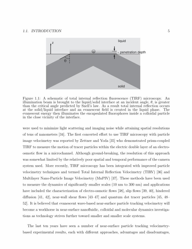
θ
z liquid
solid
~ penetration depth
Figure 1.1: A schematic of total internal reflection fluorescence (TIRF) microscopy. Anillumination beam is brought to the liquid/solid interface at an incident angle, θ, is greaterthan the critical angle predicted by Snell’s law. As a result total internal reflection occursat the solid/liquid interface and an evanescent field is created in the liquid phase. Theevanescent energy then illuminates the encapsulated fluorophores inside a colloidal particlein the close vicinity of the interface.
were used to minimize light scattering and imaging noise while attaining spatial resolutions
of tens of nanometers [34]. The first concerted effort to use TIRF microscopy with particle
image velocimetry was reported by Zettner and Yoda [35] who demonstrated prism-coupled
TIRF to measure the motion of tracer particles within the electric double layer of an electro-
osmotic flow in a microchannel. Although ground-breaking, the resolution of this approach
was somewhat limited by the relatively poor spatial and temporal performance of the camera
system used. More recently, TIRF microscopy has been integrated with improved particle
velocimetry techniques and termed Total Internal Reflection Velocimetry (TIRV) [36] and
Multilayer Nano-Particle Image Velocimetry (MnPIV) [37]. These methods have been used
to measure the dynamics of significantly smaller scales (10 nm to 300 nm) and applications
have included the characterization of electro-osmotic flows [38], slip flows [39, 40], hindered
diffusion [41, 42], near-wall shear flows [43–47] and quantum dot tracer particles [45, 48–
52]. It is believed that evanescent wave-based near-surface particle tracking velocimetry will
become a workhorse in near-surface nanofluidic, colloidal and molecular dynamics investiga-
tions as technology strives further toward smaller and smaller scale systems.
The last ten years have seen a number of near-surface particle tracking velocimetry-
based experimental results, each with different approaches, advantages and disadvantages,
6 CHAPTER 1. NEAR-SURFACE PARTICLE TRACKING VELOCIMETRY
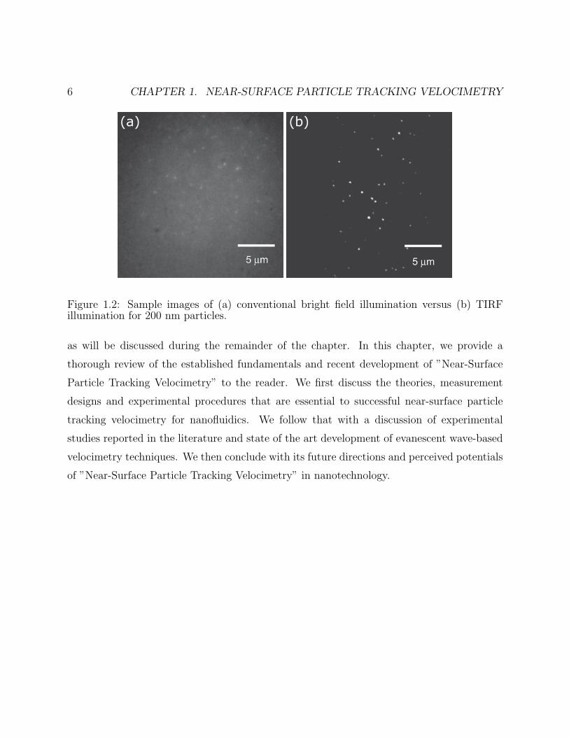
(b)(a)
Figure 1.2: Sample images of (a) conventional bright field illumination versus (b) TIRFillumination for 200 nm particles.
as will be discussed during the remainder of the chapter. In this chapter, we provide a
thorough review of the established fundamentals and recent development of ”Near-Surface
Particle Tracking Velocimetry” to the reader. We first discuss the theories, measurement
designs and experimental procedures that are essential to successful near-surface particle
tracking velocimetry for nanofluidics. We follow that with a discussion of experimental
studies reported in the literature and state of the art development of evanescent wave-based
velocimetry techniques. We then conclude with its future directions and perceived potentials
of ”Near-Surface Particle Tracking Velocimetry” in nanotechnology.
1.2. THEORETICAL CONSIDERATIONS 7
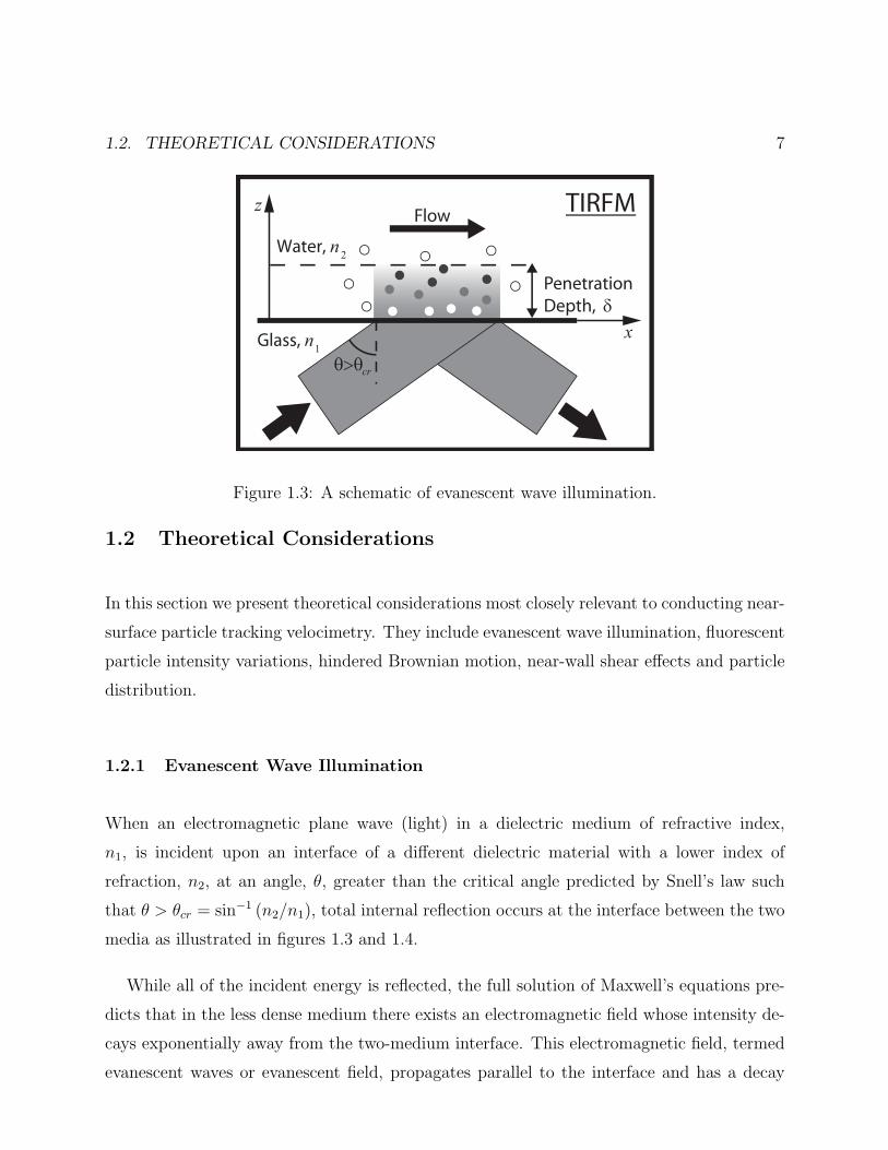
Penetration Depth, δ
θ>θcr
Water, n 2
Glass, n1
z
x
Flow TIRFM
Figure 1.3: A schematic of evanescent wave illumination.
1.2 Theoretical Considerations
In this section we present theoretical considerations most closely relevant to conducting near-
surface particle tracking velocimetry. They include evanescent wave illumination, fluorescent
particle intensity variations, hindered Brownian motion, near-wall shear effects and particle
distribution.
1.2.1 Evanescent Wave Illumination
When an electromagnetic plane wave (light) in a dielectric medium of refractive index,
n1, is incident upon an interface of a different dielectric material with a lower index of
refraction, n2, at an angle, θ, greater than the critical angle predicted by Snell’s law such
that θ > θcr = sin−1 (n2/n1), total internal reflection occurs at the interface between the two
media as illustrated in figures 1.3 and 1.4.
While all of the incident energy is reflected, the full solution of Maxwell’s equations pre-
dicts that in the less dense medium there exists an electromagnetic field whose intensity de-
cays exponentially away from the two-medium interface. This electromagnetic field, termed
evanescent waves or evanescent field, propagates parallel to the interface and has a decay
8 CHAPTER 1. NEAR-SURFACE PARTICLE TRACKING VELOCIMETRY
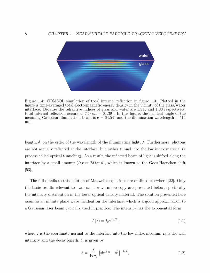
water
glass
Figure 1.4: COMSOL simulation of total internal reflection in figure 1.3. Plotted in thefigure is time-averaged total electromagnetic energy density in the vicinity of the glass/waterinterface. Because the refractive indices of glass and water are 1.515 and 1.33 respectively,total internal reflection occurs at θ > θcr = 61.39. In this figure, the incident angle of theincoming Gaussian illumination beam is θ = 64.54 and the illumination wavelength is 514nm.
length, δ, on the order of the wavelength of the illuminating light, λ. Furthermore, photons
are not actually reflected at the interface, but rather tunnel into the low index material (a
process called optical tunneling). As a result, the reflected beam of light is shifted along the
interface by a small amount (∆x ≈ 2δ tan θ), which is known as the Goos-Haenchen shift
[53].
The full details to this solution of Maxwell’s equations are outlined elsewhere [22]. Only
the basic results relevant to evanescent wave microscopy are presented below, specifically
the intensity distribution in the lower optical density material. The solution presented here
assumes an infinite plane wave incident on the interface, which is a good approximation to
a Gaussian laser beam typically used in practice. The intensity has the exponential form
I (z) = I0e−z/δ, (1.1)
where z is the coordinate normal to the interface into the low index medium, I0 is the wall
intensity and the decay length, δ, is given by
δ =λ
4πn1
[sin2 θ − n2
]−1/2, (1.2)
1.2. THEORETICAL CONSIDERATIONS 9
0 0.5 1 1.5 20
0.2
0.4
0.6
0.8
1
z/λ
Nor
mal
ized
Inte
nsity
SimulationTheory
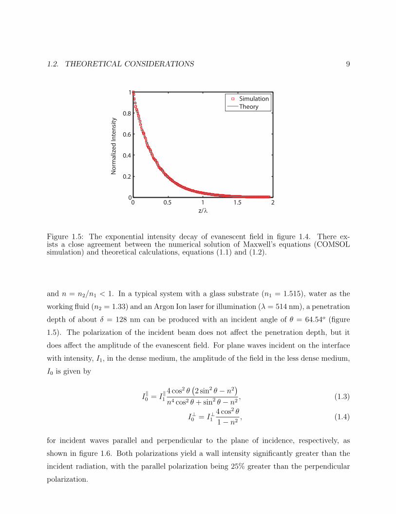
Figure 1.5: The exponential intensity decay of evanescent field in figure 1.4. There ex-ists a close agreement between the numerical solution of Maxwell’s equations (COMSOLsimulation) and theoretical calculations, equations (1.1) and (1.2).
and n = n2/n1 < 1. In a typical system with a glass substrate (n1 = 1.515), water as the
working fluid (n2 = 1.33) and an Argon Ion laser for illumination (λ = 514 nm), a penetration
depth of about δ = 128 nm can be produced with an incident angle of θ = 64.54o (figure
1.5). The polarization of the incident beam does not affect the penetration depth, but it
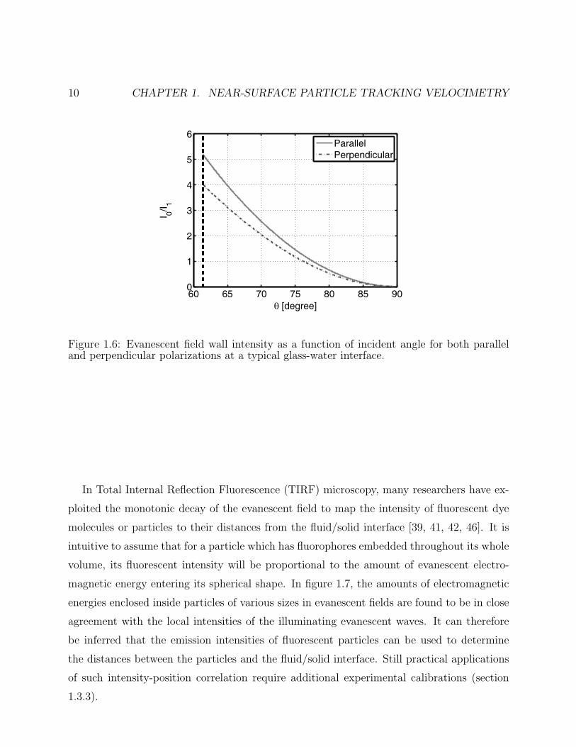
does affect the amplitude of the evanescent field. For plane waves incident on the interface
with intensity, I1, in the dense medium, the amplitude of the field in the less dense medium,
I0 is given by
I‖0 = I
‖1
4 cos2 θ(2 sin2 θ − n2
)n4 cos2 θ + sin2 θ − n2
, (1.3)
I⊥0 = I⊥14 cos2 θ
1− n2, (1.4)
for incident waves parallel and perpendicular to the plane of incidence, respectively, as
shown in figure 1.6. Both polarizations yield a wall intensity significantly greater than the
incident radiation, with the parallel polarization being 25% greater than the perpendicular
polarization.
10 CHAPTER 1. NEAR-SURFACE PARTICLE TRACKING VELOCIMETRY
60 65 70 75 80 85 900
1
2
3
4
5
6
θ [degree]
I 0/I 1
ParallelPerpendicular
Figure 1.6: Evanescent field wall intensity as a function of incident angle for both paralleland perpendicular polarizations at a typical glass-water interface.
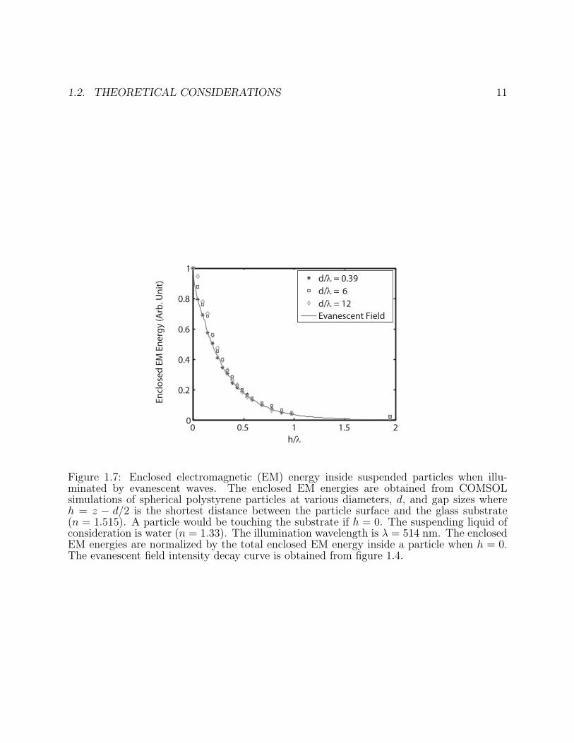
In Total Internal Reflection Fluorescence (TIRF) microscopy, many researchers have ex-
ploited the monotonic decay of the evanescent field to map the intensity of fluorescent dye
molecules or particles to their distances from the fluid/solid interface [39, 41, 42, 46]. It is
intuitive to assume that for a particle which has fluorophores embedded throughout its whole
volume, its fluorescent intensity will be proportional to the amount of evanescent electro-
magnetic energy entering its spherical shape. In figure 1.7, the amounts of electromagnetic
energies enclosed inside particles of various sizes in evanescent fields are found to be in close
agreement with the local intensities of the illuminating evanescent waves. It can therefore
be inferred that the emission intensities of fluorescent particles can be used to determine
the distances between the particles and the fluid/solid interface. Still practical applications
of such intensity-position correlation require additional experimental calibrations (section
1.3.3).
1.2. THEORETICAL CONSIDERATIONS 11
0 0.5 1 1.5 20
0.2
0.4
0.6
0.8
1
h/λ
Encl
osed
EM
Ene
rgy
(Arb
. Uni
t)
d/λ = 0.39d/λ = 6d/λ = 12Evanescent Field
Figure 1.7: Enclosed electromagnetic (EM) energy inside suspended particles when illu-minated by evanescent waves. The enclosed EM energies are obtained from COMSOLsimulations of spherical polystyrene particles at various diameters, d, and gap sizes whereh = z − d/2 is the shortest distance between the particle surface and the glass substrate(n = 1.515). A particle would be touching the substrate if h = 0. The suspending liquid ofconsideration is water (n = 1.33). The illumination wavelength is λ = 514 nm. The enclosedEM energies are normalized by the total enclosed EM energy inside a particle when h = 0.The evanescent field intensity decay curve is obtained from figure 1.4.
12 CHAPTER 1. NEAR-SURFACE PARTICLE TRACKING VELOCIMETRY
1.2.2 Fluorescent Nanoparticle Intensity Variation
When applying the intensity-distance correlation described in the previous section to an
ensemble of nanometer-sized particles that are typically used in fluid mechanics and colloid
dynamics measurements, one must consider the polydispersity of the particles and the varia-
tion of emission intensity with particle size. All commercially available polystyrene and latex
nanoparticles are manufactured with a finite size distribution where the particle radius is
specified by a mean value a0 and a coefficient of variation up to 20%. Several researchers have
attempted to compensate for this variation statistically, when making ensemble-averaged
measurements of fluorescent nanoparticles with TIRF [39, 47]. Most manufacturers impreg-
nate the volume of the polymer particles with fluorescent dye, and thus it is often assumed
that the light intensity emitted by a particle is proportional to its volume. For instance,
Huang et al. [39] proposed that the intensity of a given particle, Ip, of radius a at a distance
h from the interface is
Ip (z, a) = Ip0
(a
a0
)3
exp
[−z − a
δ
], (1.5)
where Ip0 is the intensity of a particle with a radius a0 and δ is the penetration depth of the
evanescent field.
Below, we quote results from Chew (1988) [54] for dipole radiation inside dielectric spheres
to support the claim that particle intensity is proportional to volume and demonstrate the
limits of this assumption for larger particles. Consider a dielectric sphere of radius, a,
permittivity, ε1, permeability, µ1, and index of refraction, n1 =√µ1ε1, inside of a second,
infinite dielectric medium with ε2, µ2, and n2. The radiation from an emitting dipole with
free space wavelength, λ0, will have momentum vectors, k1,2 = 2πn1,2/λ0, and subsequently,
ρ1,2 = k1,2a. The power emitted by a dipole is proportional to the dipole transition rate, R⊥,‖,
for perpendicular and parallel polarizations. These relations are provided in Chew (1988)
and are normalized by the transition rates for dipoles contained in an infinite medium 1,
R⊥,‖/R⊥,‖0 . For a distribution of dipoles, c (~r), located within the sphere, the volume averaged
emission is ⟨R⊥,‖
R⊥,‖0
⟩=
∫ (R⊥,‖/R
⊥,‖0
)c (~r) d3~r∫
c (~r) d3~r. (1.6)
1.2. THEORETICAL CONSIDERATIONS 13
The volume averaged emission for randomly oriented dipoles, R/R0, with a uniform concen-
tration distribution, c (~r) = c0, is
⟨R
R0
⟩≡ 1
3
⟨R⊥
R⊥0+ 2
R‖
R‖0
⟩= 2H
∞∑n=1
[Jn|Dn|2
+GKn
|D′n|2
], (1.7)
where
H =
√µ1ε1ε2µ2
(9ε14ρ5
1
),
G =µ1µ2
ε1ε2,
Kn =ρ3
1
2
[j2n (ρ1)− jn+1 (ρ1) jn−1 (ρ1)
],
Jn = Kn−1 − nρ1j2n (ρ1) ,
Dn = ε1jn (ρ1)[ρ2h
(1)n (ρ2)
]′ − ε2h(1)n (ρ2) [ρ1jn (ρ1)]′ ,
D′n = µ1jn (ρ1)[ρ2h
(1)n (ρ2)
]′ − µ2h(1)n (ρ2) [ρ1jn (ρ1)]′ .
Spherical Bessel functions of the first kind are denoted by jn, and spherical Hankel functions
of the first kind are denoted by h(1)n . The terms Dn and D′n are the same denominators of the
Mie scattering coefficients [55]. In the Rayleigh limit (ka 1), the transition rates become
independent of polarization and simplify greatly to
⟨R
R0
⟩=
9
(ε1/ε2 + 2)2
√ε2µ3
2
ε1µ31
. (1.8)
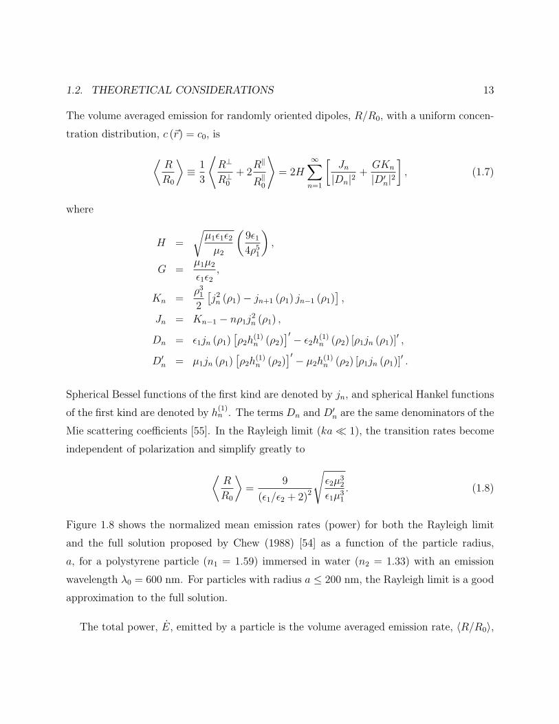
Figure 1.8 shows the normalized mean emission rates (power) for both the Rayleigh limit
and the full solution proposed by Chew (1988) [54] as a function of the particle radius,
a, for a polystyrene particle (n1 = 1.59) immersed in water (n2 = 1.33) with an emission
wavelength λ0 = 600 nm. For particles with radius a ≤ 200 nm, the Rayleigh limit is a good
approximation to the full solution.
The total power, E, emitted by a particle is the volume averaged emission rate, 〈R/R0〉,
14 CHAPTER 1. NEAR-SURFACE PARTICLE TRACKING VELOCIMETRY
0 100 200 300 400 5000
0.2
0.4
0.6
0.8
1
Radius, a [nm]
Nor
mal
ied
Mea
n R
ate
Chew (1988)Rayleigh Limit
Figure 1.8: Volume averaged emission rate for uniformly distributed, randomly orientedradiating dipoles with emission wavelength, λ0 = 600 nm, within a polystyrene sphere (n1 =1.59) immersed in water (n2 = 1.33).
scaled by the volume of a given particle
E =4
3πa3
⟨R
R0
⟩. (1.9)
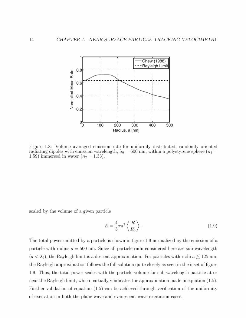
The total power emitted by a particle is shown in figure 1.9 normalized by the emission of a
particle with radius a = 500 nm. Since all particle radii considered here are sub-wavelength
(a < λ0), the Rayleigh limit is a descent approximation. For particles with radii a . 125 nm,
the Rayleigh approximation follows the full solution quite closely as seen in the inset of figure
1.9. Thus, the total power scales with the particle volume for sub-wavelength particle at or
near the Rayleigh limit, which partially vindicates the approximation made in equation (1.5).
Further validation of equation (1.5) can be achieved through verification of the uniformity
of excitation in both the plane wave and evanescent wave excitation cases.
1.2. THEORETICAL CONSIDERATIONS 15
0 100 200 300 400 5000
0.2
0.4
0.6
0.8
1
Radius, a [nm]
Tot
al E
mis
sion
Chew (1988)Rayleigh Limit
0 50 1000
0.005
0.01
0.015
0.02
0.025
0.03
Figure 1.9: Total emission (power) for uniformly distributed, randomly oriented radiatingdipoles with emission wavelength, λ0 = 600 nm, within a polystyrene sphere (n1 = 1.59)immersed in water (n2 = 1.33). For particles approaching the Rayleigh limit with radii,a ≤ 125 nm, the emitted power scales with the particle volume.
1.2.3 Hindered Brownian Motion
The Brownian motion of small particles due to molecular fluctuations is generally well un-
derstood [56] and can be significant in magnitude for nanoparticles commonly used for near-
surface particle tracking velocimetry. The random, thermal forcing of the particles is damped
by the hydrodynamic drag resulting from the surrounding solvent molecules, and the parti-
cle’s motion can be described as a diffusion process [57]:
∂p (~r, t)
∂t= ∇ · (D (~r)∇p (~r, t)) , (1.10)
where p is the probability of finding a particle at a given location, ~r, at time, t, and D is
the diffusion coefficient. For an isolated, spherical particle that is significantly larger than
the surrounding solvent molecules, the diffusion coefficient is constant and isotropic, and it
is described by the Stokes-Einstein relation [58]
D0 =kbT
ξ=
kbT
6πµa, (1.11)
16 CHAPTER 1. NEAR-SURFACE PARTICLE TRACKING VELOCIMETRY
where kb is Boltzmann’s constant, T is the absolute temperature, ξ is the drag coefficient, µ
is the dynamic viscosity of the solvent and a is the particle radius. In this case, the solution
to equation (1.10) subject to the condition p (~r, t = t0) = δ (~r − ~r0) becomes
p (~r, t) =1
8 (πD0∆t)3/2exp
[−|~r − ~r0|2
4D0∆t
], (1.12)
where ∆t = t− t0 [59].
When an isolated particle in a quiescent fluid is in the vicinity of a solid boundary,
its Brownian motion is hindered anisotropically due to an increase in hydrodynamic drag.
Several theoretical studies have accurately captured this effect for various regimes of particle
wall separation distance [15, 60–62]. The hindered diffusion coefficient in the wall-parallel
direction, Dx, is described by
Dx
D0
= 1− 9
16
(za
)−1
+1
8
(za
)−3
− 45
256
(za
)−4
− 1
16
(za
)−5
+O(za
)−6
, (1.13)
where z is the particle center distance to the wall. This is a direct result from the drag force
on a moving particle near a stationary wall in a quiescent fluid calculated by the “method
of reflections,” which is accurate far from the wall, z/a > 2 [63]. A better approximation for
small particle-wall separation distances results from an asymptotic solution for the drag force
based on lubrication theory for z/a < 2 [61]. Under these assumptions, the corresponding,
normalized diffusion coefficient is
Dx
D0
= −2[ln(za− 1)− 0.9543
][ln(za− 1)]2 − 4.325 ln
(za− 1)
+ 1.591. (1.14)
The relative hindered diffusion coefficient for a particle diffusing in the wall-normal direction,
Dz, is described by
Dz
D0
=
4
3sinhα
∞∑n=1
n (n+ 1)
(2n− 1) (2n+ 3)[2 sinh (2n+ 1)α + (2n+ 1) sinh 2α
4 sinh2(n+ 1
2
)α− (2n+ 1)2 sinh2 α
− 1
]−1
,
(1.15)
1.2. THEORETICAL CONSIDERATIONS 17
1 2 3 4 50
0.2
0.4
0.6
0.8
1
z/a
Dx,
z/D0
Dx (Method of Reflection)
Dx (Lubrication)
Dz (Brenner, 1961)
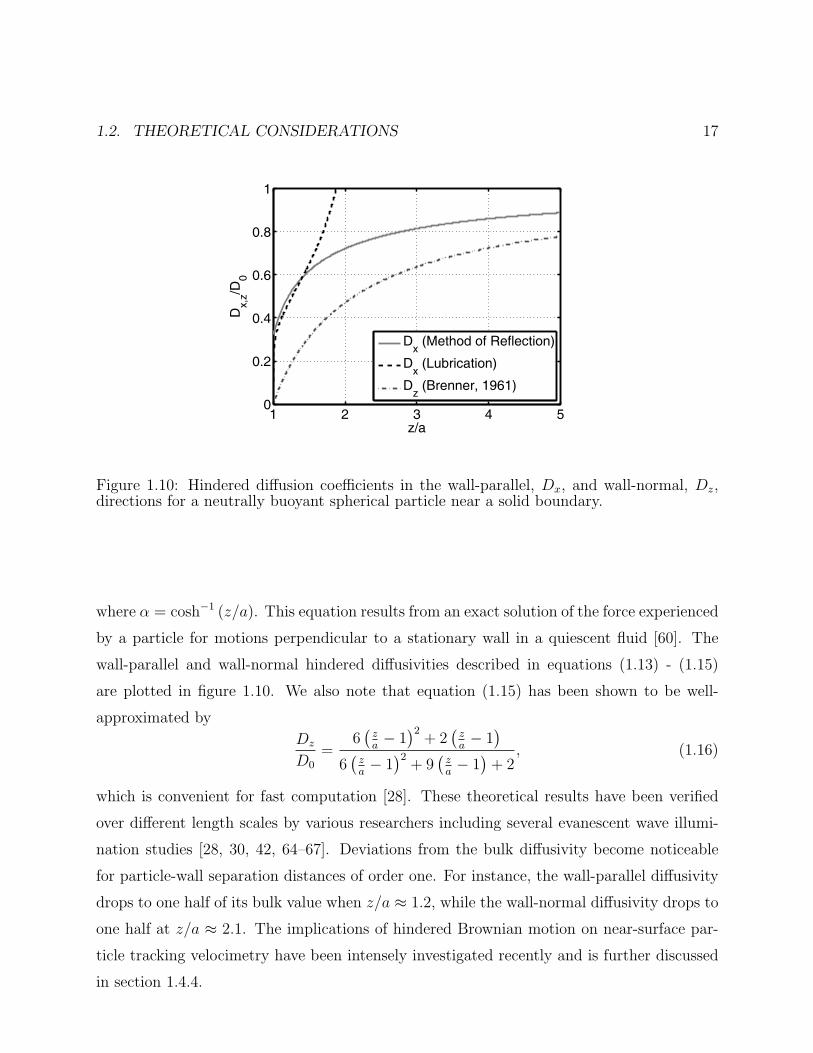
Figure 1.10: Hindered diffusion coefficients in the wall-parallel, Dx, and wall-normal, Dz,directions for a neutrally buoyant spherical particle near a solid boundary.
where α = cosh−1 (z/a). This equation results from an exact solution of the force experienced
by a particle for motions perpendicular to a stationary wall in a quiescent fluid [60]. The
wall-parallel and wall-normal hindered diffusivities described in equations (1.13) - (1.15)
are plotted in figure 1.10. We also note that equation (1.15) has been shown to be well-
approximated by
Dz
D0
=6(za− 1)2
+ 2(za− 1)
6(za− 1)2
+ 9(za− 1)
+ 2, (1.16)
which is convenient for fast computation [28]. These theoretical results have been verified
over different length scales by various researchers including several evanescent wave illumi-
nation studies [28, 30, 42, 64–67]. Deviations from the bulk diffusivity become noticeable
for particle-wall separation distances of order one. For instance, the wall-parallel diffusivity
drops to one half of its bulk value when z/a ≈ 1.2, while the wall-normal diffusivity drops to
one half at z/a ≈ 2.1. The implications of hindered Brownian motion on near-surface par-
ticle tracking velocimetry have been intensely investigated recently and is further discussed
in section 1.4.4.
18 CHAPTER 1. NEAR-SURFACE PARTICLE TRACKING VELOCIMETRY
1.2.4 Near-Wall Shear Effects
The motion of an incompressible fluid obeys the continuity condition (conservation of mass)
∇ · ~u = 0, (1.17)
where the velocity field, ~u, is divergence free. The Navier-Stokes equation governs the motion
of a viscous fluid and in the case of an incompressible fluid is
ρ
(∂~u
∂t+ ~u · ∇~u
)= −∇P + µ∇2~u, (1.18)
where ρ is the fluid density and P is the dynamic pressure. For the small Reynolds numbers
(Re 1) typical of microfluidic devices, equation 1.18 greatly reduces in complexity to
Stokes’ equation [68]:
∇P = µ∇2~u. (1.19)
Most microfabrication techniques produce microchannels with approximately rectangular
cross-sections. Thus, a useful result from equation (1.19) is the solution for the velocity
profile in a rectangular duct with height, d, and width, w, subject to the no-slip boundary
condition (~u = 0) at the walls. The laminar, unidirectional flow occurs in the pressure
gradient direction with velocity, ux, described below [59]:
ux (y, z) =1
2µ
(−∂P∂x
)[d2
4− z2 +
8
d
∞∑n=1
(−1)n cos (mz) cosh (my)
m3 cosh (mw/2)
], (1.20)
m =π (2n− 1)
d,
where the pressure gradient and volumetric flow rate, Q, are related by
Q =wd3
12µ
(−∂P∂x
)[1− 192d
π5w
∞∑n=1,3,5,...
1
n5
1− exp (−nπw/d)
1 + exp (−nπw/d)
]. (1.21)
It is well known that rigid particles tend to rotate in shear, and in the special case of a
sphere near a planar wall, additional hydrodynamic drag slows the particle’s translational
1.2. THEORETICAL CONSIDERATIONS 19
velocity below that of the local fluid velocity [15, 62]. For wide microchannels (w d) in
the very near-wall region (h d), the nearly parabolic velocity profile can be approximated
by a linear shear flow
u ≈ zS, (1.22)
where S is the shear rate. The wall-parallel drag force experienced by a neutrally buoyant,
free particle with radius a and a distance z between its center and the wall in a linear shear
flow results in a particle translational velocity, v, that is different from the fluid velocity
at the particle center’s plane. For large z/a, the particle’s translational velocity can be
estimated by the “method of reflections” [62]. This translational velocity, normalized by the
local fluid velocity at the particle’s center, is
v
zS' 1− 5
16
(za
)−3
. (1.23)
For small particle-wall separation distances (small z/a), an asymptotic solution based on
lubrication theory has also been established as
v
zS' 0.7431
0.6376− 0.2 ln(za− 1) , (1.24)
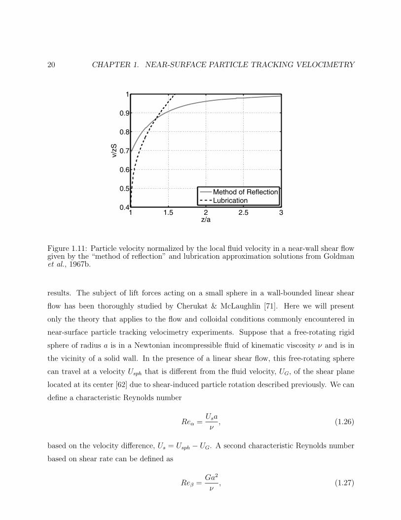
which is also normalized by the unperturbed fluid velocity at the particle’s center [62]. The
“method of reflections” solution and asymptotic lubrication solution from equations (1.23) -
(1.24) are shown in figure 1.11. Additionally, Pierres et al. [69] used a cubic approximation
to segment the solutions for intermediate values of z/a:
v
zS'(za
)−1
exp
0.68902 + 0.54756[ln(za− 1)]
+0.072332[ln(za− 1)]2
+ 0.0037644[ln(za− 1)]3.
(1.25)
Particle rotation can also induces a lifting force, which tends to make the particles migrate
away from the wall [70]. Obviously, such lift force can potentially lead to biased sampling of
local fluid velocities by the tracer particles during near-surface particle tracking velocimetry
measurements and should be cautiously treated when designing experiments and analyzing
20 CHAPTER 1. NEAR-SURFACE PARTICLE TRACKING VELOCIMETRY
1 1.5 2 2.5 30.4
0.5
0.6
0.7
0.8
0.9
1
z/a
v/zS
Method of ReflectionLubrication
Figure 1.11: Particle velocity normalized by the local fluid velocity in a near-wall shear flowgiven by the “method of reflection” and lubrication approximation solutions from Goldmanet al., 1967b.
results. The subject of lift forces acting on a small sphere in a wall-bounded linear shear
flow has been thoroughly studied by Cherukat & McLaughlin [71]. Here we will present
only the theory that applies to the flow and colloidal conditions commonly encountered in
near-surface particle tracking velocimetry experiments. Suppose that a free-rotating rigid
sphere of radius a is in a Newtonian incompressible fluid of kinematic viscosity ν and is in
the vicinity of a solid wall. In the presence of a linear shear flow, this free-rotating sphere
can travel at a velocity Usph that is different from the fluid velocity, UG, of the shear plane
located at its center [62] due to shear-induced particle rotation described previously. We can
define a characteristic Reynolds number
Reα =Usa
ν, (1.26)
based on the velocity difference, Us = Usph − UG. A second characteristic Reynolds number
based on shear rate can be defined as
Reβ =Ga2
ν, (1.27)
1.2. THEORETICAL CONSIDERATIONS 21
where G is the wall shear rate. In this geometry, the wall is considered as located in the
”inner region” of flow around the particle if Reα Ω and Reβ Ω2, where Ω ≡ a/(z − a).
For near-wall particle tracking velocimetry using nanoparticles, Reα ∼ Reβ . 10−4 while
Ω ∼ O (1), and thus the inner region theory of lift force applies.
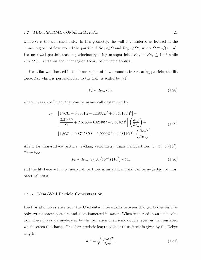
For a flat wall located in the inner region of flow around a free-rotating particle, the lift
force, FL, which is perpendicular to the wall, is scaled by [71]
FL ∼ Reα · IΩ, (1.28)
where IΩ is a coefficient that can be numerically estimated by
IΩ =[1.7631 + 0.3561Ω− 1.1837Ω2 + 0.845163Ω3
]−[
3.21439
Ω+ 2.6760 + 0.8248Ω− 0.4616Ω2
](ReβReα
)+
[1.8081 + 0.879585Ω− 1.9009Ω2 + 0.98149Ω3
](ReβReα
)2
.
(1.29)
Again for near-surface particle tracking velocimetry using nanoparticles, IΩ . O (102).
Therefore
FL ∼ Reα · IΩ .(10−4
) (102) 1, (1.30)
and the lift force acting on near-wall particles is insignificant and can be neglected for most
practical cases.
1.2.5 Near-Wall Particle Concentration
Electrostatic forces arise from the Coulombic interactions between charged bodies such as
polystyrene tracer particles and glass immersed in water. When immersed in an ionic solu-
tion, these forces are moderated by the formation of an ionic double layer on their surfaces,
which screen the charge. The characteristic length scale of these forces is given by the Debye
length,
κ−1 =
√εfε0kbT
2ce2, (1.31)
22 CHAPTER 1. NEAR-SURFACE PARTICLE TRACKING VELOCIMETRY
where ε0 is the permittivity of free space, εf is the relative permittivity of the fluid, e is the
elementary charge of an electron and c is the concentration of ions in solution [72]. In the
case of a plane-sphere geometry for like-charged objects (for example, a spherical polystyrene
particle and a flat glass substrate), the immobile substrate can exert a repulsive force on the
particle and is quantified by the potential energy of the interaction:
U el (z) = Bpse−κ(z−a). (1.32)
The magnitude of the electrostatic potential is given by
Bps = 4πεfε0a
(kbT
e
)2(ψp + 4γΩκa
1 + Ωκa
)[4 tanh
(ψs4
)], (1.33)
where γ = tanh(ψp/4
), Ω =
(ψp − 4γ
)/2γ3, ψp = ψpe/kbT and ψs = ψse/kbT [73]. ψp and
ψs represent the electric potentials of the particle and the substrate, respectively.
Contributions from attractive, short-ranged van der Waals forces, which originate from
multipole dispersion interactions [74], should also be considered when the particle-wall sep-
aration is on the order of 10 nm. The potential due to van der Waals interactions for a
plane-sphere geometry is given by
U vdw (z) = −Aps6
[a
z − a+
a
z + a+ ln
(z − az + a
)], (1.34)
where Aps is the Hamaker constant [75, 76]. The gravitational potential can also be important
for large or severely density mismatched particles. The gravitational potential of a buoyant
particle in a fluid is given by
U g (z) =4
3πa3 (ρs − ρf ) g (z − a) , (1.35)
where ρs and ρf are the densities of the sphere and fluid, respectively, and g is the acceleration
due to gravity.
Finally, optical forces due to electric field gradients from the illuminating light can trap
or push colloidal particles [77]. Below, we present an order of magnitude estimation for the
1.2. THEORETICAL CONSIDERATIONS 23
potential of a dielectric particle in a weak illuminating evanescent field typically found in
evanescent wave-based near-surface particle tracking velocimetry. Following Novotny and
Hecht [78], the force on a dipole is given by
~F = (~µ · ∇) ~E =(α~E · ∇
)~E = α∇| ~E|2. (1.36)
The dipole moment, ~µ, polarizability, α, and electric field magnitude are given by the fol-
lowing:
~µ = α~E, (1.37)
α = 4πε0a30
n2p − n2
0
n2p + 2n2
0
, (1.38)
I (z) = I0e−z/δ =
1
2cε0n0| ~E|2, (1.39)
where n0 is the index of the surrounding medium, np is the index of the particle and c is the
speed of light in a vacuum. Combining the above expressions, we can write an approximation
to the potential of a particle near an interface due to an evanescent field:
U opt ≈ −α| ~E|2 = −8πa30
cn0
n2p − n2
0
n2p + 2n2
0
I0e−z/δ, (1.40)
which is an attractive force. However, for strongly light-absorbing particles such as the
semiconductor materials found in quantum dots, this optical force can be repulsive and
more detailed analyses should be carefully carried out.
The equilibrium distribution for an ensemble of non-interacting, suspended Brownian
particles in an external potential has been shown to be given by a Boltzmann distribution
[79]. For a brief discussion, we follow Doi and Edwards (1986) [79] and consider a one-
dimensional distribution below. Fick’s law of diffusion describes the flux, j, of material
j (z, t) = −D∂p (z, t)
∂z, (1.41)
where D is the diffusion coefficient and p is the continuous probability function of finding
a particle at a location, z, in the wall-normal coordinate at time, t. In the presence of an
24 CHAPTER 1. NEAR-SURFACE PARTICLE TRACKING VELOCIMETRY
external potential, U (z), particles experience an additional force
Fz = −∂U∂z
. (1.42)
Fick’s law (equation (1.41)) is modified to reflect the additional flux induced by this force
j (z, t) = −D∂p∂z− p
ξ
∂U
∂z, (1.43)
where the drag coefficient, ξ, is related to the diffusion coefficient, D = kbT/ξ. In the steady
state, the net flux vanishes, j → 0, and the solution of equation (1.43) leads to the Boltzmann
distribution
p (z) =exp [−U (z) /kbT ]∫ z2
z1exp [−U (z) /kbT ] dz
= p0e−U/kbT , (1.44)
where p0 is a normalization constant [30] from all particles in the range z1 ≤ z ≤ z2 and U
is the total potential energy given by the sum of all potentials experienced by the particle
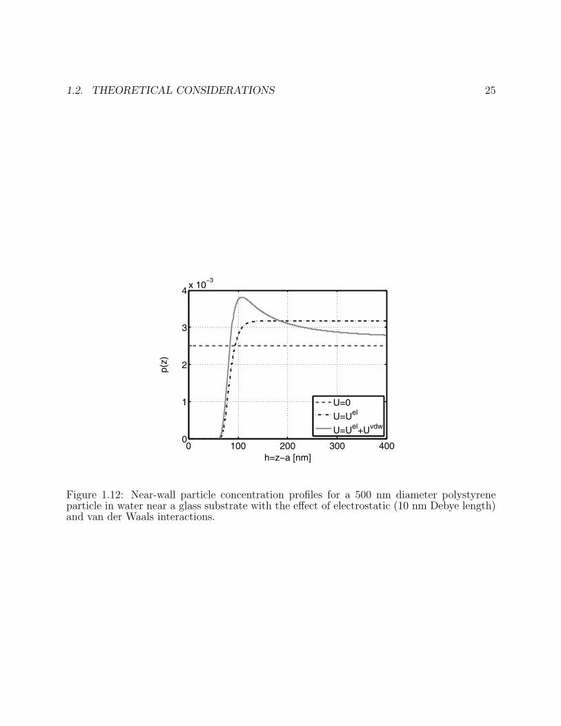
(electrostatic, van der Waals, etc.). An example illustrating the non-uniform particle con-
centrations in the near-wall region is shown in figure 1.12 for a 500 nm diameter polystyrene
particle in water near a glass substrate with a 10 nm Debye length. In this case, electrostatic
and van der Waals forces dominate, clearly forming a depletion layer within about 100 nm
of the wall. The implications of the presence of a near-surface particle depletion layer to
velocimetry accuracy has recently been investigated and reported [44, 47].
1.2. THEORETICAL CONSIDERATIONS 25
0 100 200 300 4000
1
2
3
4x 10
−3
h=z−a [nm]
p(z)
U=0
U=Uel
U=Uel+Uvdw
Figure 1.12: Near-wall particle concentration profiles for a 500 nm diameter polystyreneparticle in water near a glass substrate with the effect of electrostatic (10 nm Debye length)and van der Waals interactions.
26 CHAPTER 1. NEAR-SURFACE PARTICLE TRACKING VELOCIMETRY
1.3 Experimental Procedures
In this section, we discuss in details on the experimental procedures of conducting success-
ful evanescent wave-based near-surface particle tracking velocimetry, including selection of
experimental materials, sample preparation, optical and imaging setup, measurement cali-
bration and the particle tracking algorithm.
1.3.1 Materials and Preparations
As discussed before, creation of evanescent waves inside a microfluidic or nanofluidic channel
requires the solid substrate or the channel wall to have higher optical density than the
flowing fluid. That is, the substrate must have a higher index of refraction than the fluid
does. Furthermore, the substrate must be transparent to both the illumination and the
fluorescence emission wavelengths for high precision imaging. Examples of solid materials
that satisfy these conditions include glass (n = 1.47 - 1.65), quartz (n = 1.55), Poly-methyl
methacrylate (PMMA, n = 1.49) and other types of clear plastics. Among these, glass is the
most common choice as it is chemically inert, physically robust and optically transparent to
all visible light wavelengths (350 - 700 nm). Surface roughness of less than 10 nm is found
to be not impeding the creation of evanescent waves. However, surface waviness presents a
more critical issue as the local illumination incident angle could significantly deviate from
the predicted value and thus changes the properties of the created evanescent waves. It
should also be noted that thin-film chemical coatings of sub-wavelength thickness on the
substrate surface does not prevent creation of evanescent waves. Demonstrated examples of
coatings used in near-surface particle tracking velocimetry includes octadecyltrichorosilane
(OTS) [39, 40] and P-selectin glycoprotein ligand-1 (PSGL-1) [47] self-assembled monolayers.
Selection of the experimental fluid is typically based on the following criteria: (1) lower
refractive index than that of the solid substrate; (2) lack of chemical reactions with the solid
substrate or surface coatings; (3) availability of chemically compatible tracer particles; (4)
desired physical properties such as density, viscosity and polarity. Air and various inert gases
have the lowest refractive indices possible among fluids (n ≈ 1), but creating submicron-sized
1.3. EXPERIMENTAL PROCEDURES 27
aerosol tracer particles presents a difficult challenge. Water (n = 1.33) is the most common
choice of fluid for its chemical stability and compatibility with biochemical reagents. Other
organic and inorganic solvents such as hexane (n = 1.375) and ethanol (n = 1.36) are also
potential candidates.
A wide range of micron-sized and nanometer-sized tracer particles are commercially avail-
able for near-surface particle tracking velocimetry. For light scattering-based experiments,
metallic, glass and quartz particles should be considered as they are stronger scatterers of
evanescent waves. For fluorescence-based measurements, the list of tracer particle candidates
include fluorescent polystyrene and latex particles, fluorescently tagged macromolecules such
as Dextran and DNA, and semiconductor materials such as quantum dots. Tracer particle
properties such as density, average size and size variations, deformation tendency, potential
affinity to substrate, coagulation tendencies, chemical compatibility with fluid, and fluores-
cence quantum efficiency and wavelength should be carefully evaluated before and during
experimentation. In general, particles that have fluorophores embedded throughout its whole
volume is preferred for maximum imaging signals. Density mismatch between tracer particles
and the fluid can lead to buoyancy and sedimentation that cause velocimetry measurement
bias. These problems can be avoided if the chosen type of tracer particles satisfy the following
condition,4πa4g |ρp − ρf |
3kBT 1, (1.45)
where a is average particle radius, g is gravitational acceleration, ρp is particle density, ρf is
fluid density, kB is Boltzmann constant and T is experimental fluid temperature. Coagulation
of tracer particles also presents serious problems for particle identifications and intensity-
based 3D positioning and should avoided as much as possible. Simple sonication of particle
suspension is usually quite effective in breaking up particle clumps. Finally, the tracer
particle seeding density of the measurement suspension should be moderately low to avoid
tracking ambiguity between frames of images and assure velocimetry accuracy. A good rule
of thumb is that the average spacing (in pixels) between adjacent tracer particles in the
acquired images should be at least 5 times larger than the average particle size (also in
pixels) of the same images.
28 CHAPTER 1. NEAR-SURFACE PARTICLE TRACKING VELOCIMETRY
1.3.2 Evanescent Wave Microscopy Setup
The basic components of an evanescent wave imaging system include: a light source, condi-
tioning optics, specimen or microfluidic device, fluorescence emission imaging optics and a
camera. In reported experimental setups, light sources have included both continuous-wave
(CW) lasers (argon-ion, helium-neon) and pulsed lasers (Nd:YAG) since they produce colli-
mated, narrow wavelength-band illumination beams. Non-coherent sources (arc-lamps) are
not common because they require band pass filters for wavelength selection and the produced
light beams cannot be as perfectly collimated. However, commercial versions of lamp-based
evanescent wave microscopes are available for qualitative imaging as they are more econom-
ical than laser-based systems. Conditioning optics are used to create the angle of incidence
necessary for total internal reflection and are of two types: prism-based and objective-based
[21]. Prism-based evanescent imaging systems are typically laboratory-built and low cost.
A prism is placed in contact with the sample substrate which the illumination light beam
is coupled into by inserting an immersion medium in between. The illumination beam is
focused through the prism onto the substrate at an angle greater than the critical angle such
that the substrate then becomes a waveguide where evanescent waves are generated along
its surface (figure 1.13(a)). An air- or a water-immersion, long working-distance objective is
often used for imaging to prevent decoupling of the guided wave from the substrate into the
objective. Detailed prism and microscope configurations can be found in [21]. In contrast,
objective-based evanescent wave imaging is used exclusively with fluorescence and requires a
high numerical aperture objective (NA > 1.4) to achieve the large incident angles required
for total internal reflection (figure 1.13(b)). These objectives are usually high magnification
(60× ≤M ≤ 100×) and oil-immersion. In this method, a collimated illumination light beam
is focused onto the back focal plane of the objective and translated off the optical axis of
the objective to create the required large incident angle. The emitted fluorescence of tracer
particles is collected by the objective and recorded by a camera as in typical fluorescence
microscopy. To prevent the returning excitation light from being recorded by the camera,
spectral filtering with dichroic mirrors and filters is employed.
Another advantage of evanescent wave imaging to note is that its imaging depth provides
significantly greater imaging resolution than the diffraction-limited depth of field, DOF , of
1.3. EXPERIMENTAL PROCEDURES 29
Waveguide
Prism
Illumination Beam
EvanescentField
Fluorescent Nanoparticle
Microscope Objective
Evanescent Field
Fluorescent Nanoparticles
Substrate
Microscope Objective
θ
(a)
(b)
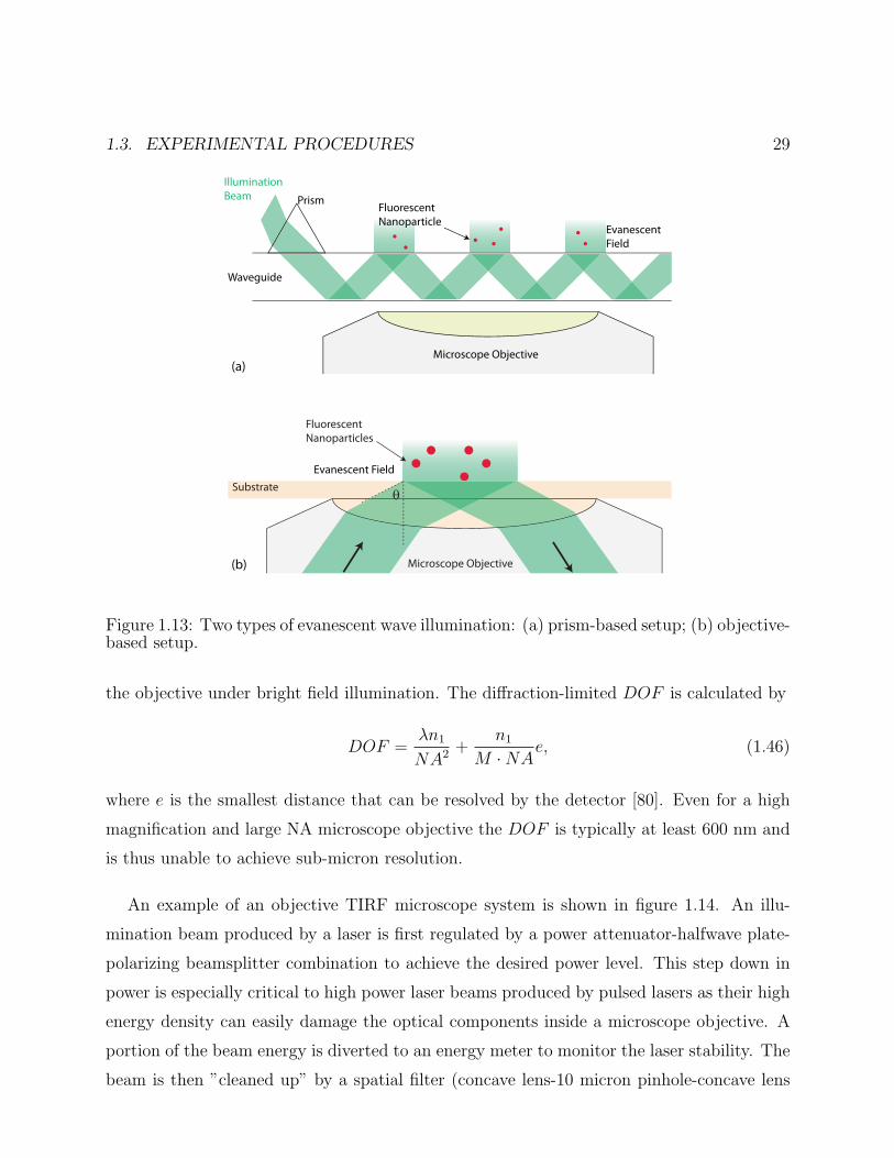
Figure 1.13: Two types of evanescent wave illumination: (a) prism-based setup; (b) objective-based setup.
the objective under bright field illumination. The diffraction-limited DOF is calculated by
DOF =λn1
NA2 +n1
M ·NAe, (1.46)
where e is the smallest distance that can be resolved by the detector [80]. Even for a high
magnification and large NA microscope objective the DOF is typically at least 600 nm and
is thus unable to achieve sub-micron resolution.
An example of an objective TIRF microscope system is shown in figure 1.14. An illu-
mination beam produced by a laser is first regulated by a power attenuator-halfwave plate-
polarizing beamsplitter combination to achieve the desired power level. This step down in
power is especially critical to high power laser beams produced by pulsed lasers as their high
energy density can easily damage the optical components inside a microscope objective. A
portion of the beam energy is diverted to an energy meter to monitor the laser stability. The
beam is then ”cleaned up” by a spatial filter (concave lens-10 micron pinhole-concave lens

30 CHAPTER 1. NEAR-SURFACE PARTICLE TRACKING VELOCIMETRY
ICCD
Laser
100X, NA = 1.45Objective lens
Dichroic mirror andBarrier filter
Microchannel
Convex lens
Pulse generator
Computer 1360 x 1036x 12 bit
PowerAttenuator
Half-waveplate
Data Acquisition
Mirror
Convex Lens
10 micron pinholeConvex Lens
PolarizingBeamsplitter
Energy Meter
Figure 1.14: A schematic of objective-based TIRF microscope setup.
combination) before being directed through an NA1.45 100X oil-immersion microscope ob-
jective at an angle that creates evanescent waves inside a microchannel. Fluorescent images
of near-surface tracer particles are captured by the same microscope objective and screened
by a dichroic mirror and a barrier filter before being projected onto an intensified CCD cam-
era (ICCD), capable of recording extremely low intensity events. A TTL pulse generator is
used to synchronize laser firing and ICCD image acquisitions to ensure precise control imag-
ing timing. The energy of the illuminating laser beam cam also be recorded simultaneously
with each image acquisition to account for illuminating energy fluctuation, if necessary.
Recent research literature has shown that objective-based TIRF microscopy systems are
becoming much more common for experimental microfluidic and nanofluidic investigations.
Extremely high signal-to-noise ratio images can be produced with proper alignment and
conditioning of the incident beam, and good control over the fluorescence imaging. Here,
we discuss general methodologies for alignment and beam conditioning as well as supply the
relevant details to reconstruct a proven system with an inverted epi-fluorescent microscope.
The procedure, which follows, is valid for both pulsed and continuous wave (CW) lasers.
Caution should always be exercised when working with high power laser. Proper eye protec-
1.3. EXPERIMENTAL PROCEDURES 31
(a)(b)
(c) (d) (e)
(f)
(g)
Lase
rTo
Mic
rosc
ope
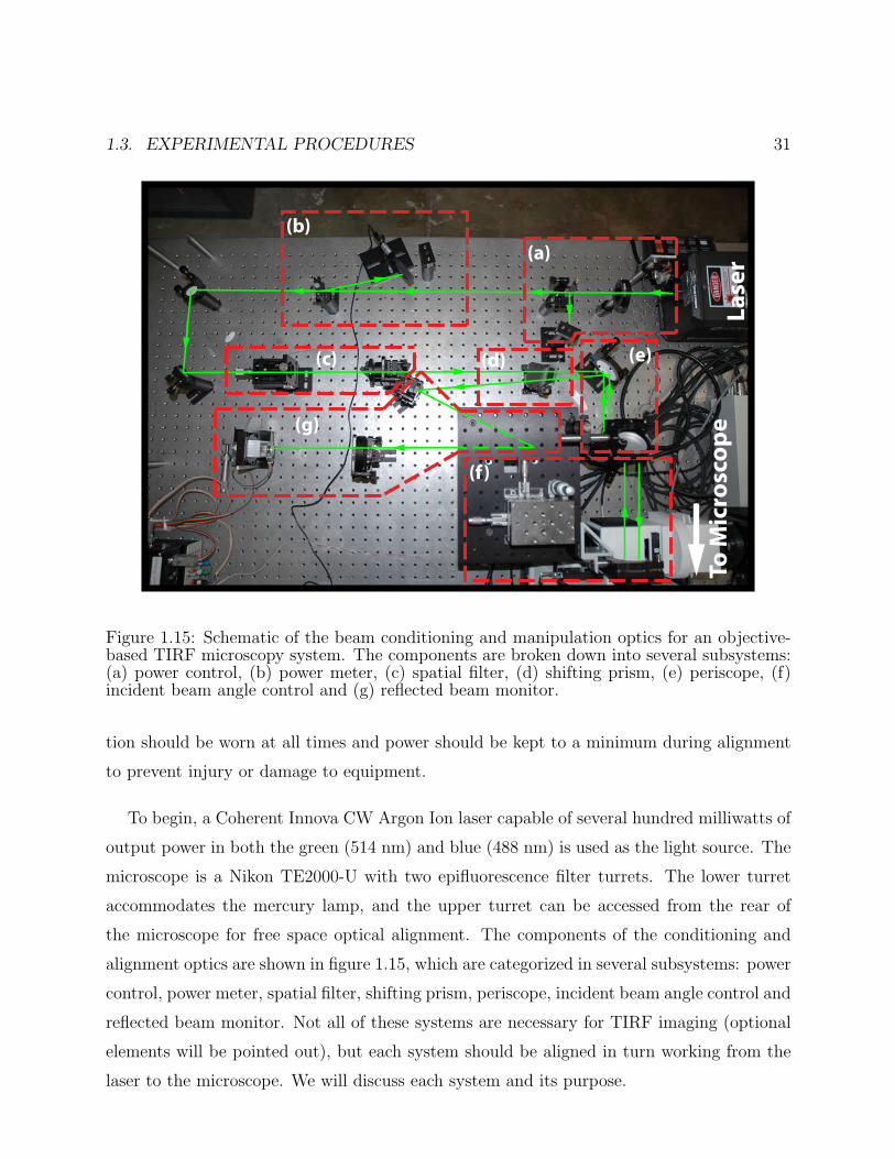
Figure 1.15: Schematic of the beam conditioning and manipulation optics for an objective-based TIRF microscopy system. The components are broken down into several subsystems:(a) power control, (b) power meter, (c) spatial filter, (d) shifting prism, (e) periscope, (f)incident beam angle control and (g) reflected beam monitor.
tion should be worn at all times and power should be kept to a minimum during alignment
to prevent injury or damage to equipment.
To begin, a Coherent Innova CW Argon Ion laser capable of several hundred milliwatts of
output power in both the green (514 nm) and blue (488 nm) is used as the light source. The
microscope is a Nikon TE2000-U with two epifluorescence filter turrets. The lower turret
accommodates the mercury lamp, and the upper turret can be accessed from the rear of
the microscope for free space optical alignment. The components of the conditioning and
alignment optics are shown in figure 1.15, which are categorized in several subsystems: power
control, power meter, spatial filter, shifting prism, periscope, incident beam angle control and
reflected beam monitor. Not all of these systems are necessary for TIRF imaging (optional
elements will be pointed out), but each system should be aligned in turn working from the
laser to the microscope. We will discuss each system and its purpose.
32 CHAPTER 1. NEAR-SURFACE PARTICLE TRACKING VELOCIMETRY
The laser should always be operated near maximum power for the best thermal stability.
As a safety mechanism and control, a mechanical beam chopper is placed directly in front
of the laser aperture (figure 1.15(a)). It is used as a beam stop for warm-up and can be
controlled electronically for periodic modulation of the beam if desired. Next, the already
vertically polarized laser passes through a half-wave plate to rotate the polarization to an
arbitrary angle. The wave plate in combination with the polarizing beam splitter that follows
allows one to continuously vary the evanescent wave intensity of the TIRF microscopy system,
while maintaining maximum operating power at the laser. By rotating the polarization, the
vertical component is allowed to propagate along its original path through the beam splitter,
while the horizontally polarized light (excess power) is dumped to a beam stop toward the
interior of the optical table. Next, the useful component of the beam is split again for power
measurement (figure 1.15(b)). With a fairly sensitive meter, a few hundred microwatts is
sufficient for accurate measurement without being wasteful of the excitation power.
Two mirrors are now used redirect the beam toward the back of the microscope and align
the beam conveniently along the optical table bolt pattern using two irises (not shown).
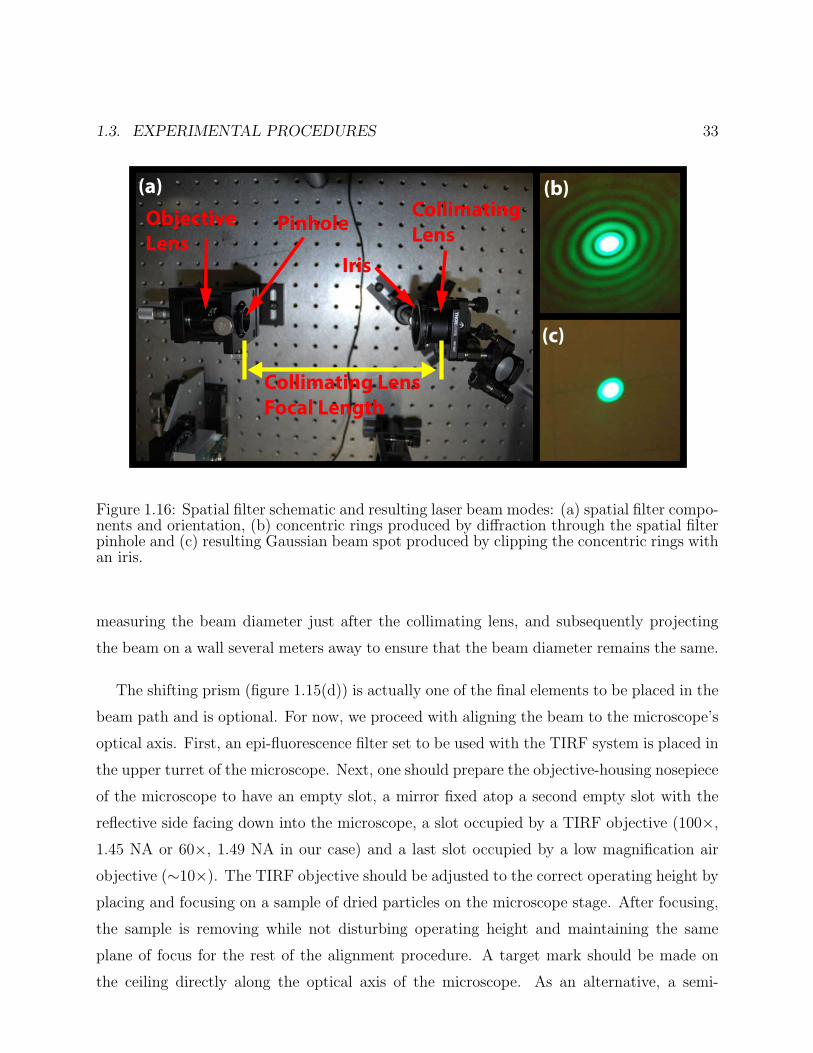
After referencing the beam to the table, a spatial filter is implemented to obtain the TEM00
mode and expand the laser beam diameter (figure 1.15(c)). The spatial filter movement
containing an objective lens (f = 8 mm) and pinhole (∼20 µm) is first aligned to be co-
linear with the beam, as shown in figure 1.16(a). When properly aligned, the spatial filter
movement should produce a diverging, concentric ring pattern that is symmetric and bright
(figure 1.16(b)), while maintaining the beam propagation to the original trajectory along the
optical table. To collimate and expand the beam, a lens (f ≈ 20 cm) is placed roughly one
focal length away from the pinhole. The focal length of the lens and divergence angle of the
expanding beam will determine the final beam diameter, which is about one centimeter in
our case. Next, an adjustable iris is placed close to the collimating lens, with sufficient space
in between for further adjustment of the lens (figure 1.16(a)). The iris is aligned to block
all of the rings from the diverging beam by narrowing the opening of the iris to the first
minimum of the concentric ring pattern. If successful, one should now be left with a very
“clean” Gaussian beam spot as shown in figure 1.16(c). Finally, fine tune the position of the
collimating lens such that the beam is collimated and again maintains the original trajectory
along the bolt pattern of the optical table. One can determine if the beam is collimated by
1.3. EXPERIMENTAL PROCEDURES 33
(b)
(c)
(a)ObjectiveLens
Pinhole
Iris
CollimatingLens
Collimating Lens Focal Length
Figure 1.16: Spatial filter schematic and resulting laser beam modes: (a) spatial filter compo-nents and orientation, (b) concentric rings produced by diffraction through the spatial filterpinhole and (c) resulting Gaussian beam spot produced by clipping the concentric rings withan iris.
measuring the beam diameter just after the collimating lens, and subsequently projecting
the beam on a wall several meters away to ensure that the beam diameter remains the same.
The shifting prism (figure 1.15(d)) is actually one of the final elements to be placed in the
beam path and is optional. For now, we proceed with aligning the beam to the microscope’s
optical axis. First, an epi-fluorescence filter set to be used with the TIRF system is placed in
the upper turret of the microscope. Next, one should prepare the objective-housing nosepiece
of the microscope to have an empty slot, a mirror fixed atop a second empty slot with the
reflective side facing down into the microscope, a slot occupied by a TIRF objective (100×,
1.45 NA or 60×, 1.49 NA in our case) and a last slot occupied by a low magnification air
objective (∼10×). The TIRF objective should be adjusted to the correct operating height by
placing and focusing on a sample of dried particles on the microscope stage. After focusing,
the sample is removing while not disturbing operating height and maintaining the same
plane of focus for the rest of the alignment procedure. A target mark should be made on
the ceiling directly along the optical axis of the microscope. As an alternative, a semi-
34 CHAPTER 1. NEAR-SURFACE PARTICLE TRACKING VELOCIMETRY
transparent optical element (diffuser glass) with a cross-hair can be fitted to the empty slot
of the nosepiece.
The nosepiece should now be rotated to the empty slot. Two large, five centimeter
diameter periscope mirrors (figure 1.15(e)) are placed at the rear of the microscope such
that the laser beam is directed into the microscope, reflected off the dichroic mirror and
projected through the empty slot of the nosepiece and onto the ceiling. Large mirrors are
chosen for the periscope to capture the reflected beam since the incident and reflected beams
will not travel on the same axis once the system is shifted into the TIRF mode later. In
the mean time, the goal of the current task is to align the laser beam to be co-linear with
the microscope’s optical axis. The next step is to rotate the nosepiece to the up-side-down
mirror position. At this time, one should see a reflected beam exit the rear of the microscope.
By use only one of the periscope mirrors, the incident and reflected beam are to be aligned
to become co-linear at the rear of the microscope. Next, the nosepiece is rotated back to the
open position while the incident beam is redirected to the target mark on the ceiling using the
second periscope mirror. This process should be repeated until the optical axes are co-linear
and the incident beam lands on the ceiling target without any further periscope adjustments
needed. The optional shifting prism (figure 1.15(d)), which is simply a rectangular solid
piece of glass, can now be inserted between the collimating lens of the spatial filter and the
periscope. The prism is adjusted and rotated until the incident beam hits the target mark
on the ceiling and the optical axes of the incident and reflected beams are again co-linear.
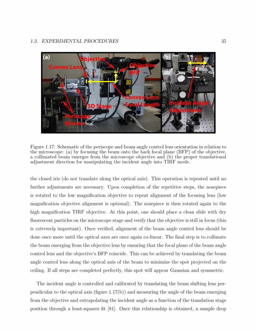
The incident beam angle control (figure 1.15(f)), which consists of a large, five centimeter
lens (f ≈ 30 cm) on a two-axes rotational lens mount on a three-axes translational stage,
should be placed between the periscope and microscope at approximately one focal distance
away from the objective’s back focal plane (BFP) as shown in figure 1.17(a). Again, the
large lens is used to accommodate the shifted reflection of the incident beam in the TIRF
mode. By placing a closed iris adjacent to the lens, one can align the optical axis of the
lens to be co-linear with the existing beam path. The iris is then opened and the rotational
mount is adjusted to align the beam to the marked target on the ceiling through the open
slot in the nosepiece. Subsequently, the iris is again closed and the lens is translated on the
plane perpendicular to the laser beam optical axis to align the beam through the center of
1.3. EXPERIMENTAL PROCEDURES 35
(a) (b)
Convex Lens
3D Stage
PeriscopeMirrors
Objective BFP
Objective
Incident AngleAdjustment
Convex LensFocal Length
Figure 1.17: Schematic of the periscope and beam angle control lens orientation in relation tothe microscope: (a) by focusing the beam onto the back focal plane (BFP) of the objective,a collimated beam emerges from the microscope objective and (b) the proper translationaladjustment direction for manipulating the incident angle into TIRF mode.
the closed iris (do not translate along the optical axis). This operation is repeated until no
further adjustments are necessary. Upon completion of the repetitive steps, the nosepiece
is rotated to the low magnification objective to repeat alignment of the focusing lens (low
magnification objective alignment is optional). The nosepiece is then rotated again to the
high magnification TIRF objective. At this point, one should place a clean slide with dry
fluorescent particles on the microscope stage and verify that the objective is still in focus (this
is extremely important). Once verified, alignment of the beam angle control lens should be
done once more until the optical axes are once again co-linear. The final step is to collimate
the beam emerging from the objective lens by ensuring that the focal plane of the beam angle
control lens and the objective’s BFP coincide. This can be achieved by translating the beam
angle control lens along the optical axis of the beam to minimize the spot projected on the
ceiling. If all steps are completed perfectly, this spot will appear Gaussian and symmetric.
The incident angle is controlled and calibrated by translating the beam shifting lens per-
pendicular to the optical axis (figure 1.17(b)) and measuring the angle of the beam emerging
from the objective and extrapolating the incident angle as a function of the translation stage
position through a least-squares fit [81]. Once this relationship is obtained, a sample drop
36 CHAPTER 1. NEAR-SURFACE PARTICLE TRACKING VELOCIMETRY
of fluid containing fluorescent tracer particles is placed on the slide and the beam angle is
adjusted until evanescent waves are created in the fluid phase (again, remember to wear
proper eye protection here). The experimentally determined angle should be compared with
the predicted TIRF angle to verify the calibration. Last, the shifting prism can be rotated
to center the evanescent waves spot in the eyepiece field of view. Although this final adjust-
ment is optional, if it is performed the incident angle should be re-calibrated. The final and
optional system for the evanescent wave microscopy system is the reflected beam monitoring
system (figure 1.15(g)), which can be used to monitor changes in the total internal reflection
conditions if necessary.
1.3.3 Fluorescent Particle Intensity and Particle Position
As mentioned before, the monotonic decay of the evanescent field have been exploited to map
the intensities of fluorescent tracer particles to their distances from the fluid-solid interface
[39, 41, 42, 46]. Using this information, one can use a calibrated ratiometric fluorescence
intensity to track particle motions three-dimensionally. Although this method sounds the-
oretically feasible, successful use of this technique in practice requires precise knowledge of
the illumination beam incident angle and a solution of Maxwell’s equation for an evanescent
field in a three media system (substrate, fluid and tracer particles) which can be difficult
to express explicitly. However, an experimental method can be devised to obtain a ratio-
metric relation between particle emission intensity and its distance to the glass surface such
as that shown in figure 1.4. In our TIRF calibration, we attached individual fluorescent
nanoparticles to polished fine tips of graphite rods, which were translated perpendicularly
through the evanescent field to the glass substrate with a 0.4-nm precision translation stage
(MadCity Nano-OP25). Multiple images of the attached particles were captured at trans-
lational increments of 20 nanometers. The intensity values of the imaged particles were
averaged and fitted to a two-dimensional Gaussian function to find their center intensities.
The process was repeated several times with different particles. This procedure produces an
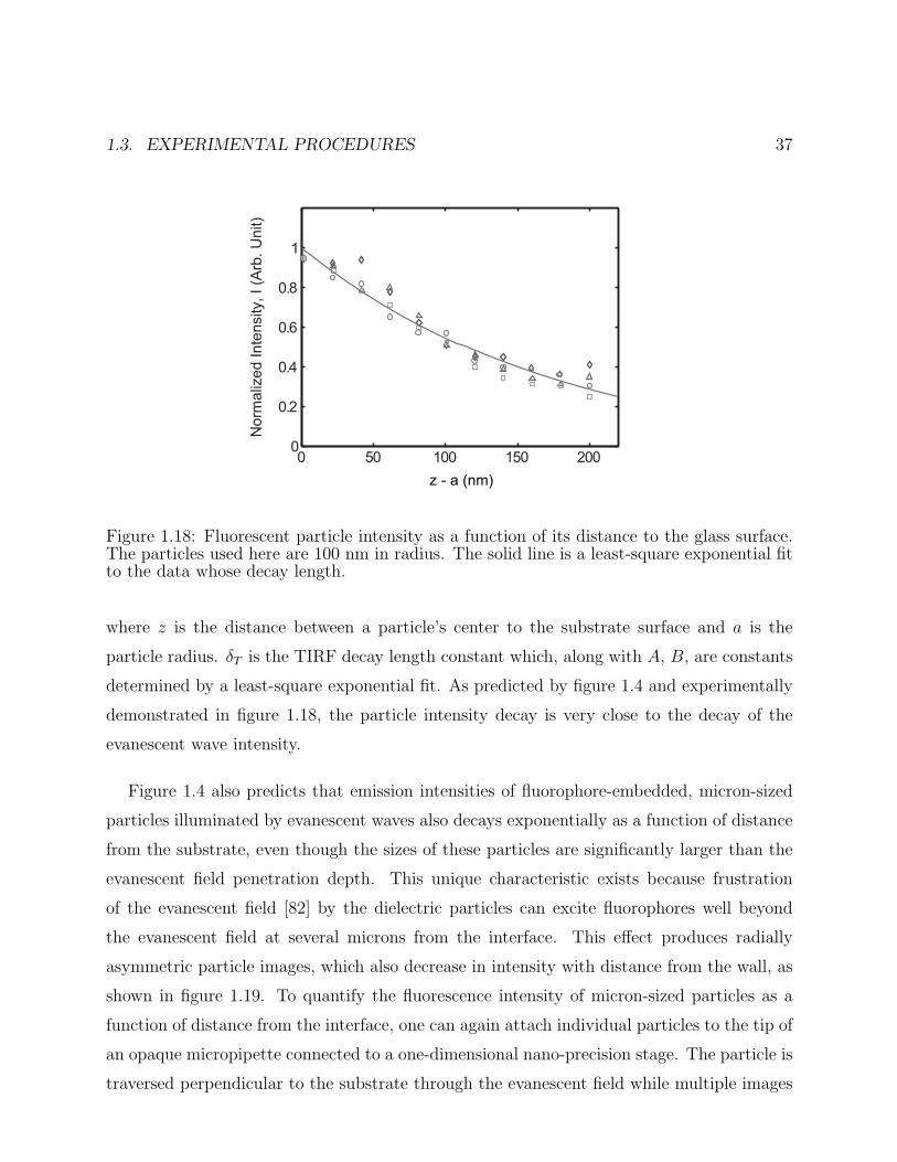
intensity-distance correlation such as one shown in figure 1.18:
I = Ae− z−a
δT +B, (1.47)
1.3. EXPERIMENTAL PROCEDURES 37
0 50 100 150 2000
0.2
0.4
0.6
0.8
1N
orm
aliz
ed In
tens
ity, I
(Arb
. Uni
t)
z - a (nm)
Figure 1.18: Fluorescent particle intensity as a function of its distance to the glass surface.The particles used here are 100 nm in radius. The solid line is a least-square exponential fitto the data whose decay length.
where z is the distance between a particle’s center to the substrate surface and a is the
particle radius. δT is the TIRF decay length constant which, along with A, B, are constants
determined by a least-square exponential fit. As predicted by figure 1.4 and experimentally
demonstrated in figure 1.18, the particle intensity decay is very close to the decay of the
evanescent wave intensity.
Figure 1.4 also predicts that emission intensities of fluorophore-embedded, micron-sized
particles illuminated by evanescent waves also decays exponentially as a function of distance
from the substrate, even though the sizes of these particles are significantly larger than the
evanescent field penetration depth. This unique characteristic exists because frustration
of the evanescent field [82] by the dielectric particles can excite fluorophores well beyond
the evanescent field at several microns from the interface. This effect produces radially
asymmetric particle images, which also decrease in intensity with distance from the wall, as
shown in figure 1.19. To quantify the fluorescence intensity of micron-sized particles as a
function of distance from the interface, one can again attach individual particles to the tip of
an opaque micropipette connected to a one-dimensional nano-precision stage. The particle is
traversed perpendicular to the substrate through the evanescent field while multiple images
38 CHAPTER 1. NEAR-SURFACE PARTICLE TRACKING VELOCIMETRY
x [µm]
y [µ
m]
z=0 nm
0 5 10
0
5
10
x [µm]y
[µm
]
z=74 nm
0 5 100
5
10
x [µm]
y [µ
m]
z=130 nm
0 5 10
0
5
10
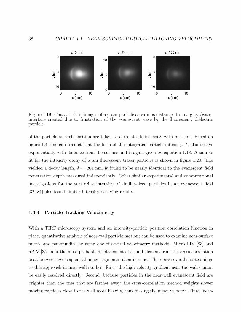
Figure 1.19: Characteristic images of a 6 µm particle at various distances from a glass/waterinterface created due to frustration of the evanescent wave by the fluorescent, dielectricparticle.
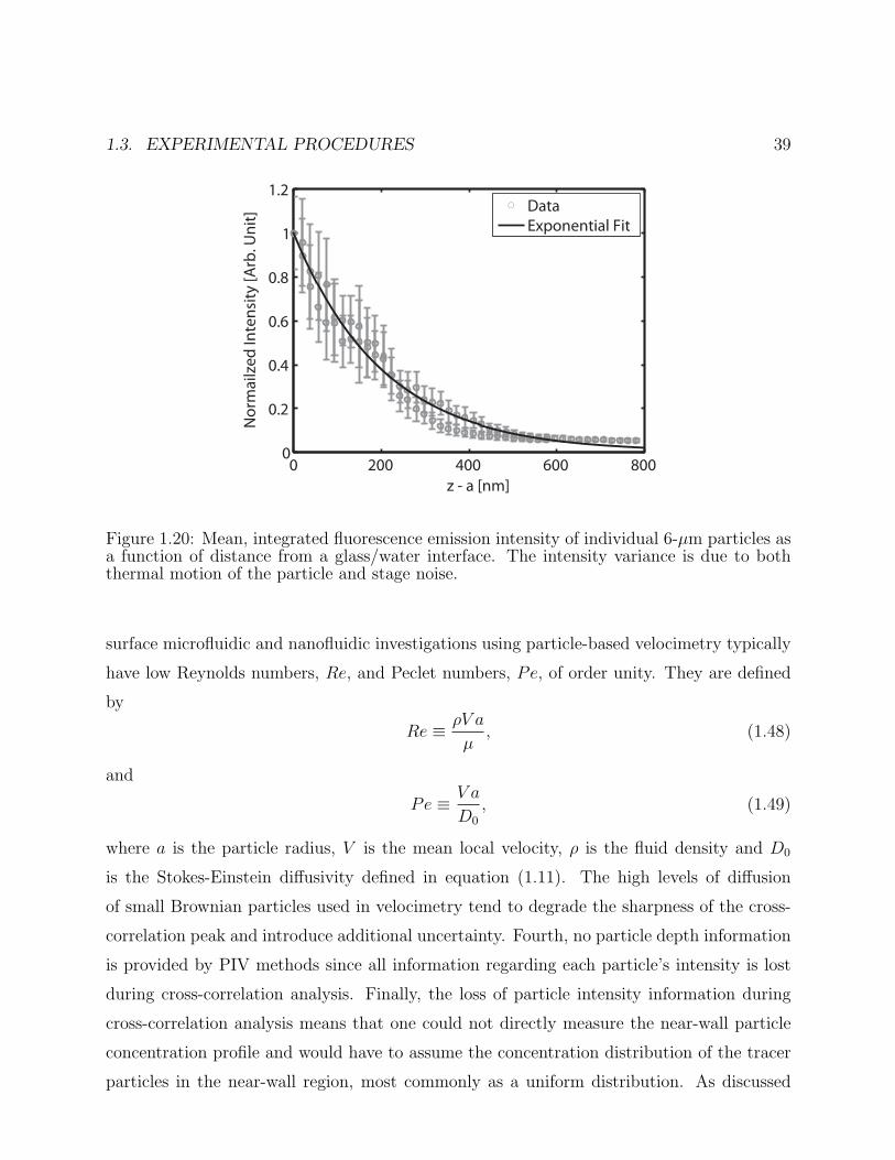
of the particle at each position are taken to correlate its intensity with position. Based on
figure 1.4, one can predict that the form of the integrated particle intensity, I, also decays
exponentially with distance from the surface and is again given by equation 1.18. A sample
fit for the intensity decay of 6-µm fluorescent tracer particles is shown in figure 1.20. The
yielded a decay length, δT =204 nm, is found to be nearly identical to the evanescent field
penetration depth measured independently. Other similar experimental and computational
investigations for the scattering intensity of similar-sized particles in an evanescent field
[32, 81] also found similar intensity decaying results.
1.3.4 Particle Tracking Velocimetry
With a TIRF microscopy system and an intensity-particle position correlation function in
place, quantitative analysis of near-wall particle motions can be used to examine near-surface
micro- and nanofluidics by using one of several velocimetry methods. Micro-PIV [83] and
nPIV [35] infer the most probable displacement of a fluid element from the cross-correlation
peak between two sequential image segments taken in time. There are several shortcomings
to this approach in near-wall studies. First, the high velocity gradient near the wall cannot
be easily resolved directly. Second, because particles in the near-wall evanescent field are
brighter than the ones that are farther away, the cross-correlation method weights slower
moving particles close to the wall more heavily, thus biasing the mean velocity. Third, near-
1.3. EXPERIMENTAL PROCEDURES 39
0 200 400 600 8000
0.2
0.4
0.6
0.8
1
1.2
z - a [nm]
Nor
mai
lzed
Inte
nsity
[Arb
. Uni
t]
DataExponential Fit
Figure 1.20: Mean, integrated fluorescence emission intensity of individual 6-µm particles asa function of distance from a glass/water interface. The intensity variance is due to boththermal motion of the particle and stage noise.
surface microfluidic and nanofluidic investigations using particle-based velocimetry typically
have low Reynolds numbers, Re, and Peclet numbers, Pe, of order unity. They are defined
by
Re ≡ ρV a
µ, (1.48)
and
Pe ≡ V a
D0
, (1.49)
where a is the particle radius, V is the mean local velocity, ρ is the fluid density and D0
is the Stokes-Einstein diffusivity defined in equation (1.11). The high levels of diffusion
of small Brownian particles used in velocimetry tend to degrade the sharpness of the cross-
correlation peak and introduce additional uncertainty. Fourth, no particle depth information
is provided by PIV methods since all information regarding each particle’s intensity is lost
during cross-correlation analysis. Finally, the loss of particle intensity information during
cross-correlation analysis means that one could not directly measure the near-wall particle
concentration profile and would have to assume the concentration distribution of the tracer
particles in the near-wall region, most commonly as a uniform distribution. As discussed

40 CHAPTER 1. NEAR-SURFACE PARTICLE TRACKING VELOCIMETRY
in section 1.2.5, such an assumption can significantly deviate from the actual concentration
profile and lead to analysis bias.
Due to the statistical nature of colloidal dynamics, one method to unmask the true physics
hiding behind the randomness of Brownian motion is individual particle tracking [84]. As
shown in section 1.3.3, the intensities of micron-sized and nanoparticles decay exponentially
away from the fluid-solid interface with decay lengths similar to that of the illuminating
evanescent waves [32, 39, 42, 46]. This makes it possible to discern the height of a particle
from the substrate surface based on its intensity, and has been applied to track particle
motions three-dimensionally [42, 47]. Although there have been some attempts to evaluate
cross-correlations over multiple particle layers [37] within the evanescent field, many chal-
lenges still remain. Tracking individual particles to resolve near-surface velocities remains a
much more direct method to investigate near-wall dynamics. Below we will discuss the most
common algorithms for tracking near-wall particles with details to help the readers develop
their own image analysis codes.
In particle tracking velocimetry (PTV), bright particles with intensities above a pre-
determined threshold value are first identified in a series of images. To track particle motions,
all particle locations from two or more successive video frames must be identified to good
accuracy, most commonly through identification of the particle center positions. For micron-
sized particles or larger, this is typically done by finding their intensity centroids through
weighted-function particle image analysis. For sub-wavelength particles, center positions are
found by fitting a two dimensional Gaussian distribution to the imaged diffraction limited
spots of the tracer particles [78, 85]. A two-dimensional Gaussian curve fit closely approxi-
mates the actual point-spread function of nanoparticle intensities near their peaks and allows
one to locate the particle center coordinates with sub-pixel resolution. At this point, it is
also critical to distinguish real particles from noise signals as noise tracking will unneces-
sarily corrupt the obtained motion statistics. This is typically accomplished by building an
additional abnormality detection algorithm into the particle identification code. Examples
include detecting the particle shapes and sizes based on their images [36].
It is important to point out that the determination of an intensity threshold during
1.3. EXPERIMENTAL PROCEDURES 41
ObservationDepth
Substrate
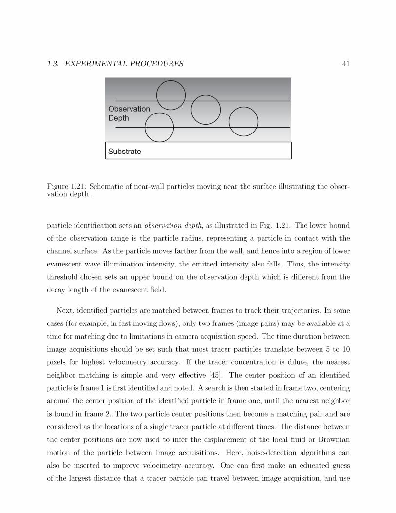
Figure 1.21: Schematic of near-wall particles moving near the surface illustrating the obser-vation depth.
particle identification sets an observation depth, as illustrated in Fig. 1.21. The lower bound
of the observation range is the particle radius, representing a particle in contact with the
channel surface. As the particle moves farther from the wall, and hence into a region of lower
evanescent wave illumination intensity, the emitted intensity also falls. Thus, the intensity
threshold chosen sets an upper bound on the observation depth which is different from the
decay length of the evanescent field.
Next, identified particles are matched between frames to track their trajectories. In some
cases (for example, in fast moving flows), only two frames (image pairs) may be available at a
time for matching due to limitations in camera acquisition speed. The time duration between
image acquisitions should be set such that most tracer particles translate between 5 to 10
pixels for highest velocimetry accuracy. If the tracer concentration is dilute, the nearest
neighbor matching is simple and very effective [45]. The center position of an identified
particle is frame 1 is first identified and noted. A search is then started in frame two, centering
around the center position of the identified particle in frame one, until the nearest neighbor
is found in frame 2. The two particle center positions then become a matching pair and are
considered as the locations of a single tracer particle at different times. The distance between
the center positions are now used to infer the displacement of the local fluid or Brownian
motion of the particle between image acquisitions. Here, noise-detection algorithms can
also be inserted to improve velocimetry accuracy. One can first make an educated guess
of the largest distance that a tracer particle can travel between image acquisition, and use
42 CHAPTER 1. NEAR-SURFACE PARTICLE TRACKING VELOCIMETRY
this distance as the radial limit of nearest neighbor search. If the nearest neighbor search
done in frame 2 for a particle identified in frame 1 is beyond this set limit, one can safely
assume that this ”particle” is probably mis-identified and is most likely a noise rather than
an actual tracer. Secondly, if more than two signals in frame 2 can be matched to a particle
identified in frame 1 using the above criteria, it is advised to discard displacement information
provided by this particle. This is because the probabilistic nature of Brownian motion makes
it impossible to resolve this matching ambiguity with any kind of certainty. It should be
noted that the image acquisitions, particle identifications and tracking processes should be
repeated for a large number of times until the number of tracked trajectories becomes a
statistically sample size. It is recommended that at least 1000 successful trackings should
be obtained for each experimental condition.
Clearly many of the tracking ambiguities and unwanted photon noises can be avoided if the
tracer particle density is low. Therefore, the tracer particle density should be kept minimal
while still capturing a good number of successful trackings from each image pair. For less than
perfect tracer particle seeding conditions, several variations of the basic tracking algorithm
have been proposed. For large Peclet numbers (less significant particle Brownian motions),
a multiple matching method may be useful [86]. However, for small Peclet numbers or
highly concentrated particle solutions, a statistical tracking method [49] or a neural network
matching algorithm [41, 87] might be advantageous. In the case that a multiple-frame image
sequence is available, there is some benefit to using window shifting and predictor corrector
methods [87], but only for large Peclet number.
Once the ensemble particle displacements are measured, the individual intensities of
matched particles can provide information about the particle distance to the substrate sur-
face as mentioned previously. Colloidal particles typically have a large diameter size variation
(3% to 20%) that can bias the interpretation of intensity to distance. Since particle intensity
can also be a function of particle size as discussed in [54, 55, 88] and in section 1.2.2, a large
particle far from the wall can appear to have the same intensity as a small particle near
the wall [39, 47]. Caution must be exercised when inferring a particle’s distance from the
substrate from its intensity.
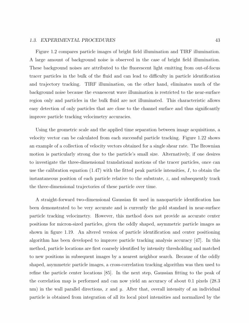
1.3. EXPERIMENTAL PROCEDURES 43
Figure 1.2 compares particle images of bright field illumination and TIRF illumination.
A large amount of background noise is observed in the case of bright field illumination.
These background noises are attributed to the fluorescent light emitting from out-of-focus
tracer particles in the bulk of the fluid and can lead to difficulty in particle identification
and trajectory tracking. TIRF illumination, on the other hand, eliminates much of the
background noise because the evanescent wave illumination is restricted to the near-surface
region only and particles in the bulk fluid are not illuminated. This characteristic allows
easy detection of only particles that are close to the channel surface and thus significantly
improve particle tracking velocimetry accuracies.
Using the geometric scale and the applied time separation between image acquisitions, a
velocity vector can be calculated from each successful particle tracking. Figure 1.22 shows
an example of a collection of velocity vectors obtained for a single shear rate. The Brownian
motion is particularly strong due to the particle’s small size. Alternatively, if one desires
to investigate the three-dimensional translational motions of the tracer particles, once can
use the calibration equation (1.47) with the fitted peak particle intensities, I, to obtain the
instantaneous position of each particle relative to the substrate, z, and subsequently track
the three-dimensional trajectories of these particle over time.
A straight-forward two-dimensional Gaussian fit used in nanoparticle identification has
been demonstrated to be very accurate and is currently the gold standard in near-surface
particle tracking velocimetry. However, this method does not provide as accurate center
positions for micron-sized particles, given the oddly shaped, asymmetric particle images as
shown in figure 1.19. An altered version of particle identification and center positioning
algorithm has been developed to improve particle tracking analysis accuracy [47]. In this
method, particle locations are first coarsely identified by intensity thresholding and matched
to new positions in subsequent images by a nearest neighbor search. Because of the oddly
shaped, asymmetric particle images, a cross-correlation tracking algorithm was then used to
refine the particle center locations [85]. In the next step, Gaussian fitting to the peak of
the correlation map is performed and can now yield an accuracy of about 0.1 pixels (28.3
nm) in the wall parallel directions, x and y. After that, overall intensity of an individual
particle is obtained from integration of all its local pixel intensities and normalized by the
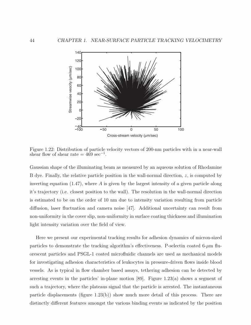
44 CHAPTER 1. NEAR-SURFACE PARTICLE TRACKING VELOCIMETRY
100 50 0 50 10040
20
0
20
40
60
80
100
120
140
Cross-stream velocity (μm/sec)
Str
eam
wis
e ve
ocity
(μm
/sec
)
Figure 1.22: Distribution of particle velocity vectors of 200-nm particles with in a near-wallshear flow of shear rate = 469 sec−1.
Gaussian shape of the illuminating beam as measured by an aqueous solution of Rhodamine
B dye. Finally, the relative particle position in the wall-normal direction, z, is computed by
inverting equation (1.47), where A is given by the largest intensity of a given particle along
it’s trajectory (i.e. closest position to the wall). The resolution in the wall-normal direction
is estimated to be on the order of 10 nm due to intensity variation resulting from particle
diffusion, laser fluctuation and camera noise [47]. Additional uncertainty can result from
non-uniformity in the cover slip, non-uniformity in surface coating thickness and illumination
light intensity variation over the field of view.
Here we present our experimental tracking results for adhesion dynamics of micron-sized
particles to demonstrate the tracking algorithm’s effectiveness. P-selectin coated 6-µm flu-
orescent particles and PSGL-1 coated microfluidic channels are used as mechanical models
for investigating adhesion characteristics of leukocytes in pressure-driven flows inside blood
vessels. As is typical in flow chamber based assays, tethering adhesion can be detected by
arresting events in the particles’ in-plane motion [89]. Figure 1.23(a) shows a segment of
such a trajectory, where the plateaus signal that the particle is arrested. The instantaneous
particle displacements (figure 1.23(b)) show much more detail of this process. There are
distinctly different features amongst the various binding events as indicated by the position
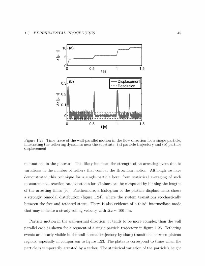
1.3. EXPERIMENTAL PROCEDURES 45
0 0.5 1 1.5
0
0.1
0.2
0.3
t [s]
Δx [μ
m]
DisplacementResolution
0 0.5 1 1.50
5
10
t [s]
x [μ
m]
(a)
(b)
Figure 1.23: Time trace of the wall-parallel motion in the flow direction for a single particle,illustrating the tethering dynamics near the substrate: (a) particle trajectory and (b) particledisplacement
fluctuations in the plateaus. This likely indicates the strength of an arresting event due to
variations in the number of tethers that combat the Brownian motion. Although we have
demonstrated this technique for a single particle here, from statistical averaging of such
measurements, reaction rate constants for off-times can be computed by binning the lengths
of the arresting times [90]. Furthermore, a histogram of the particle displacements shows
a strongly bimodal distribution (figure 1.24), where the system transitions stochastically
between the free and tethered states. There is also evidence of a third, intermediate mode
that may indicate a steady rolling velocity with ∆x ∼ 100 nm.
Particle motion in the wall-normal direction, z, tends to be more complex than the wall
parallel case as shown for a segment of a single particle trajectory in figure 1.25. Tethering
events are clearly visible in the wall-normal trajectory by sharp transitions between plateau
regions, especially in comparison to figure 1.23. The plateaus correspond to times when the
particle is temporarily arrested by a tether. The statistical variation of the particle’s height
46 CHAPTER 1. NEAR-SURFACE PARTICLE TRACKING VELOCIMETRY
−100 0 100 200 3000
0.05
0.1
0.15
0.2
0.25
0.3
∆x [nm]
Figure 1.24: A histogram of the wall-parallel particle displacements for the trajectory of atypical particle. The bimodal nature of the histogram demonstrates the fraction of time thatthe particle is tethered versus free.
during tethering events contains additional information about the tether stiffness, which may
also be examined.
We end the Experimental Procedure section with some words on system evaluation and
testing. If one follows the procedures on constructing a TIRF microscope system, setting up a
intensity-position calibration component using a nanometer-precision translation stage, and
developing a particle tracking velocimetry software to conduct near-surface particle tracking
velocimetry, it would then be necessary to test and evaluate the performance of this home-
made system, both on functionality and accuracy. In our opinion, the simplest evaluation
experiment that one can conduct is an experimental verification of Brownian motion. The
tracer particles, in quiescent fluid, will undergo hindered Brownian motion in the vicinity
of a solid substrate. Since the theory of hindered Brownian motion is quite well established
(see section 1.2.3), quantitative observations of the tracer micro- or nanoparticles using near-
surface particle tracking velocimetry can be easily compared with theories to determine if the
experimental setup and the analysis software is truly functioning with the expected precision
and accuracy. Many of the images and results shown in this section should provide sufficient
examples for one to make a proper evaluation.
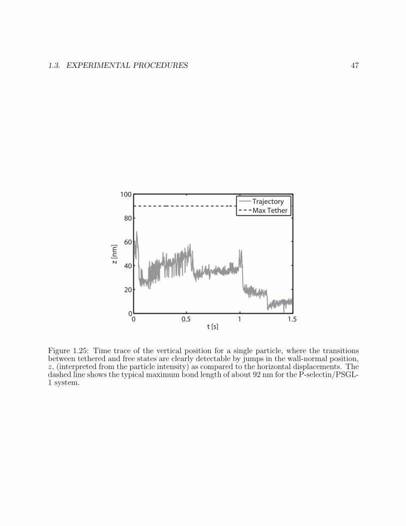
1.3. EXPERIMENTAL PROCEDURES 47
0 0.5 1 1.50
20
40
60
80
100
t [s]
z [n
m]
TrajectoryMax Tether
Figure 1.25: Time trace of the vertical position for a single particle, where the transitionsbetween tethered and free states are clearly detectable by jumps in the wall-normal position,z, (interpreted from the particle intensity) as compared to the horizontal displacements. Thedashed line shows the typical maximum bond length of about 92 nm for the P-selectin/PSGL-1 system.
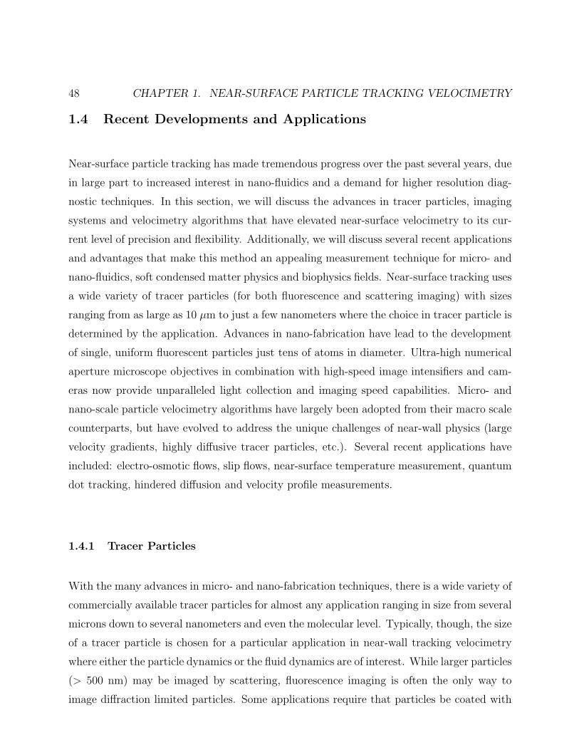
48 CHAPTER 1. NEAR-SURFACE PARTICLE TRACKING VELOCIMETRY
1.4 Recent Developments and Applications
Near-surface particle tracking has made tremendous progress over the past several years, due
in large part to increased interest in nano-fluidics and a demand for higher resolution diag-
nostic techniques. In this section, we will discuss the advances in tracer particles, imaging
systems and velocimetry algorithms that have elevated near-surface velocimetry to its cur-
rent level of precision and flexibility. Additionally, we will discuss several recent applications
and advantages that make this method an appealing measurement technique for micro- and
nano-fluidics, soft condensed matter physics and biophysics fields. Near-surface tracking uses
a wide variety of tracer particles (for both fluorescence and scattering imaging) with sizes
ranging from as large as 10 µm to just a few nanometers where the choice in tracer particle is
determined by the application. Advances in nano-fabrication have lead to the development
of single, uniform fluorescent particles just tens of atoms in diameter. Ultra-high numerical
aperture microscope objectives in combination with high-speed image intensifiers and cam-
eras now provide unparalleled light collection and imaging speed capabilities. Micro- and
nano-scale particle velocimetry algorithms have largely been adopted from their macro scale
counterparts, but have evolved to address the unique challenges of near-wall physics (large
velocity gradients, highly diffusive tracer particles, etc.). Several recent applications have
included: electro-osmotic flows, slip flows, near-surface temperature measurement, quantum
dot tracking, hindered diffusion and velocity profile measurements.
1.4.1 Tracer Particles
With the many advances in micro- and nano-fabrication techniques, there is a wide variety of
commercially available tracer particles for almost any application ranging in size from several
microns down to several nanometers and even the molecular level. Typically, though, the size
of a tracer particle is chosen for a particular application in near-wall tracking velocimetry
where either the particle dynamics or the fluid dynamics are of interest. While larger particles
(> 500 nm) may be imaged by scattering, fluorescence imaging is often the only way to
image diffraction limited particles. Some applications require that particles be coated with
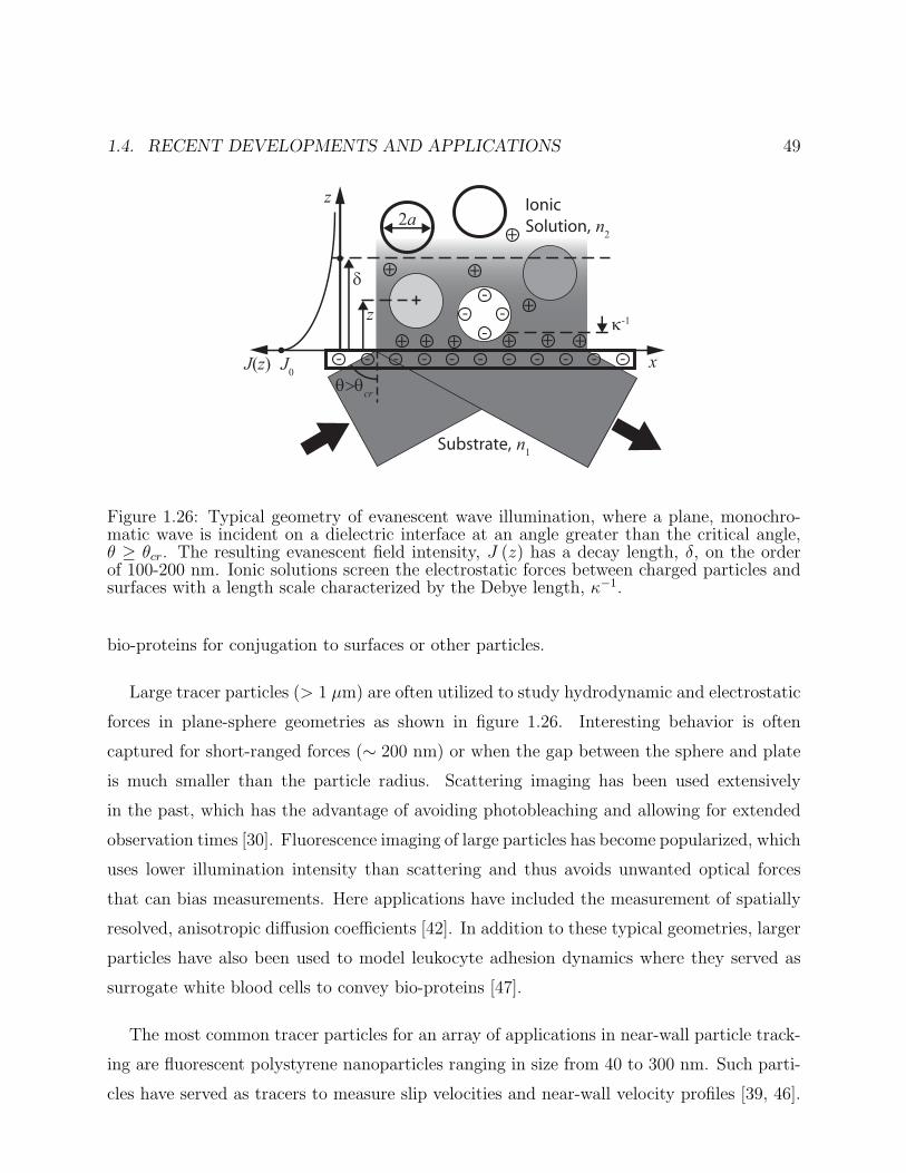
1.4. RECENT DEVELOPMENTS AND APPLICATIONS 49
θ>θcr
IonicSolution, n2
Substrate, n1
z
xJ(z) J0
δ
z
2a
+- - ------- - -
-- -
+ +++ +κ-1
+
+
++
-
Figure 1.26: Typical geometry of evanescent wave illumination, where a plane, monochro-matic wave is incident on a dielectric interface at an angle greater than the critical angle,θ ≥ θcr. The resulting evanescent field intensity, J (z) has a decay length, δ, on the orderof 100-200 nm. Ionic solutions screen the electrostatic forces between charged particles andsurfaces with a length scale characterized by the Debye length, κ−1.
bio-proteins for conjugation to surfaces or other particles.
Large tracer particles (> 1 µm) are often utilized to study hydrodynamic and electrostatic
forces in plane-sphere geometries as shown in figure 1.26. Interesting behavior is often
captured for short-ranged forces (∼ 200 nm) or when the gap between the sphere and plate
is much smaller than the particle radius. Scattering imaging has been used extensively
in the past, which has the advantage of avoiding photobleaching and allowing for extended
observation times [30]. Fluorescence imaging of large particles has become popularized, which
uses lower illumination intensity than scattering and thus avoids unwanted optical forces
that can bias measurements. Here applications have included the measurement of spatially
resolved, anisotropic diffusion coefficients [42]. In addition to these typical geometries, larger
particles have also been used to model leukocyte adhesion dynamics where they served as
surrogate white blood cells to convey bio-proteins [47].
The most common tracer particles for an array of applications in near-wall particle track-
ing are fluorescent polystyrene nanoparticles ranging in size from 40 to 300 nm. Such parti-
cles have served as tracers to measure slip velocities and near-wall velocity profiles [39, 46].
50 CHAPTER 1. NEAR-SURFACE PARTICLE TRACKING VELOCIMETRY
Over the past five years, semiconductor nanocrystals or quantum dots (QDs) have attracted
increasing attention as extremely small, bright and robust tracer particles for near-wall par-
ticle tracking. QDs are single fluorophores with reasonable quantum efficiencies and fluores-
cence lifetimes similar to conventional fluorophores, but with significantly higher resistance
to photo-bleaching [91]. They exhibit several qualities beneficial to nano-scale velocimetry
including small diameters ranging from 5 nm to 20 nm, a narrow and finely tunable emis-
sion wavelength, and even temperature sensing abilities [51]. However, single QDs have a
significantly lower emission intensity as compared to much larger polystyrene particles con-
taining several thousand fluorophores. Additionally, their emission can fluctuate randomly
(figure 1.27), which is known as fluorescence intermittency or “blinking” [92]. The first
practical demonstrations using QDs in aqueous solutions for velocimetry purposes used ei-
ther extremely dilute solutions [48] or statistical velocimetry algorithms [49] to negotiate
the necessarily long exposure times and high diffusivities. Applications include near wall
velocity bias measurements, high speed imaging, and simultaneous temperature and velocity
measurements. Hybrid particles consisting of 50 nm polystyrene particles conjugated with
a series of quantum dots also show promise as small, yet extremely bright tracer particles
[93].
1.4.2 Imaging Systems
Although the basic list of components for evanescent wave imaging systems (light source,
conditioning optics, specimen or microfluidic device, fluorescence emission imaging optics and
a camera) have remained unchanged for some time, vast improvements in the quality and
implementation of those components have translated into marked scientific achievements.
Laser sources have diminished significantly in size with increasing stability and tunability.
The conditioning optics used to create the angle of incidence necessary for total internal
reflection are still primarily prism-based or objective-based with widely varying components
[21]. Prism-based systems are still typically home-built with no significant recent advances
in technology. In contrast, objective-based imaging has benefited greatly from advances
in high magnification, high numerical aperture oil immersion objectives. Most recently,
extremely large numerical apertures NA > 1.49 have become commercially available to
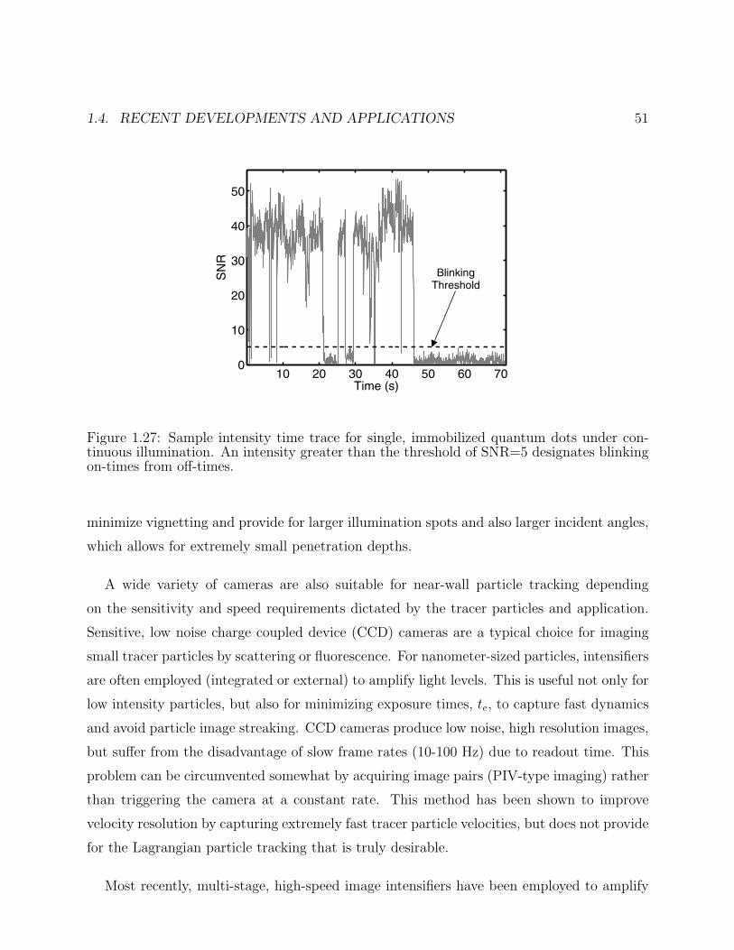
1.4. RECENT DEVELOPMENTS AND APPLICATIONS 51
10 20 30 40 50 60 700
10
20
30
40
50
Time (s)
SN
R
BlinkingThreshold
Figure 1.27: Sample intensity time trace for single, immobilized quantum dots under con-tinuous illumination. An intensity greater than the threshold of SNR=5 designates blinkingon-times from off-times.
minimize vignetting and provide for larger illumination spots and also larger incident angles,
which allows for extremely small penetration depths.
A wide variety of cameras are also suitable for near-wall particle tracking depending
on the sensitivity and speed requirements dictated by the tracer particles and application.
Sensitive, low noise charge coupled device (CCD) cameras are a typical choice for imaging
small tracer particles by scattering or fluorescence. For nanometer-sized particles, intensifiers
are often employed (integrated or external) to amplify light levels. This is useful not only for
low intensity particles, but also for minimizing exposure times, te, to capture fast dynamics
and avoid particle image streaking. CCD cameras produce low noise, high resolution images,
but suffer from the disadvantage of slow frame rates (10-100 Hz) due to readout time. This
problem can be circumvented somewhat by acquiring image pairs (PIV-type imaging) rather
than triggering the camera at a constant rate. This method has been shown to improve
velocity resolution by capturing extremely fast tracer particle velocities, but does not provide
for the Lagrangian particle tracking that is truly desirable.
Most recently, multi-stage, high-speed image intensifiers have been employed to amplify
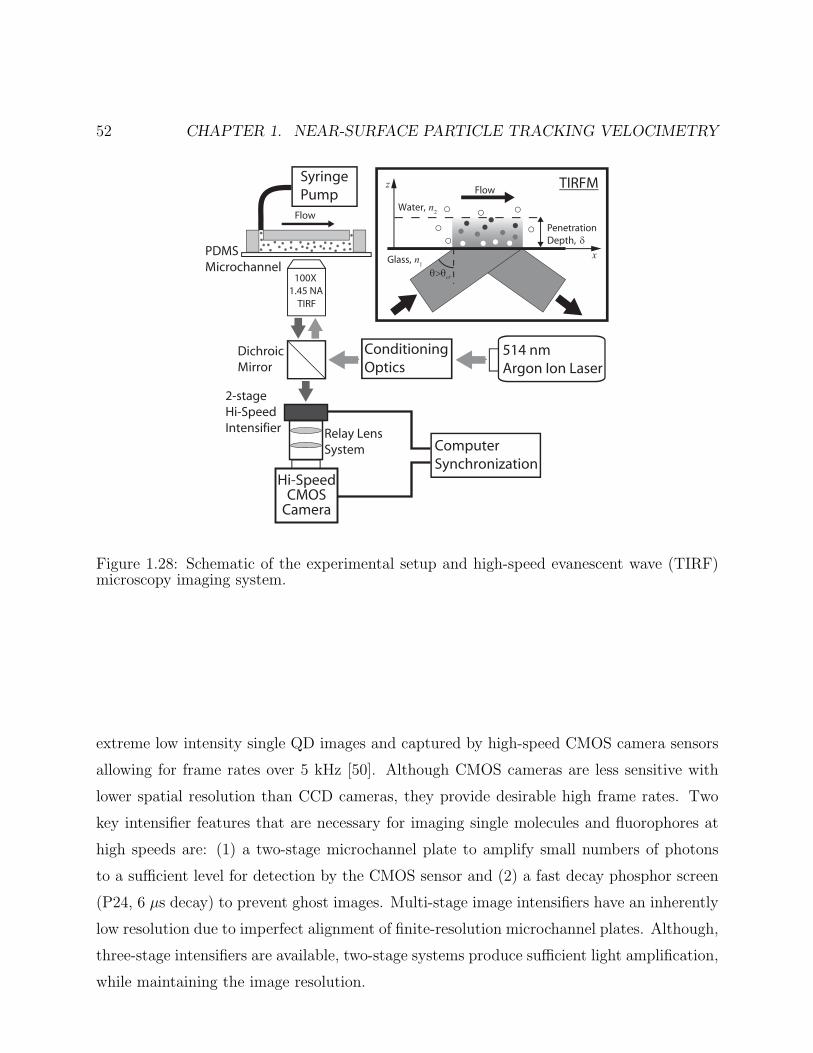
52 CHAPTER 1. NEAR-SURFACE PARTICLE TRACKING VELOCIMETRY
514 nm Argon Ion Laser
ComputerSynchronization
Hi-SpeedCMOS
Camera
DichroicMirror
PDMSMicrochannel
Flow
ConditioningOptics
SyringePump
1.45 NA100X
TIRF
Penetration Depth, δ
θ>θcr
Water, n2
Glass, n1
z
x
Flow TIRFM
Relay LensSystem
2-stageHi-SpeedIntensifier
Figure 1.28: Schematic of the experimental setup and high-speed evanescent wave (TIRF)microscopy imaging system.
extreme low intensity single QD images and captured by high-speed CMOS camera sensors
allowing for frame rates over 5 kHz [50]. Although CMOS cameras are less sensitive with
lower spatial resolution than CCD cameras, they provide desirable high frame rates. Two
key intensifier features that are necessary for imaging single molecules and fluorophores at
high speeds are: (1) a two-stage microchannel plate to amplify small numbers of photons
to a sufficient level for detection by the CMOS sensor and (2) a fast decay phosphor screen
(P24, 6 µs decay) to prevent ghost images. Multi-stage image intensifiers have an inherently
low resolution due to imperfect alignment of finite-resolution microchannel plates. Although,
three-stage intensifiers are available, two-stage systems produce sufficient light amplification,
while maintaining the image resolution.
1.4. RECENT DEVELOPMENTS AND APPLICATIONS 53
1.4.3 Tracking Algorithms
Near-wall particle velocimetry algorithms have largely been adopted from macro-scale algo-
rithms and are of two types: (i) particle image velocimetry (PIV) methods and (ii) particle
tracking velocimetry (PTV). PIV methods use cross-correlation techniques to determine the
most probable displacement for a grouping of tracer particles suspended in fluid [94]. This
yields an instantaneous snap-shot of the spatially resolved velocity field (Eulerian descrip-
tion). Conversely, PTV algorithms identify distinct, individual particles and follow their
positions in time (Lagrangian description) [87]. Both techniques have been adapted to suit
micro- and nano-fluidics, and here, in particular, we will discuss the various benefits and
costs in relation to near-surface velocimetry.
PIV Methods
Micro-scale PIV (µPIV) techniques are used to measure fluid velocity fields with length scales
L < 1 mm [83]. The depth of field of the imaging objective defines a measurement plane with
a typical thickness of 500 nm [80]. Nano-scale PIV (nPIV) uses the same cross-correlation
analysis techniques as its micro-scale counterpart, but instead uses the penetration depth
of the evanescent wave intensity to define an imaging plane with 100 ≤ δ ≤ 200 nm of the
surface [35]. This provides obvious advantages over µPIV including a more defined imaging
plane and significantly better signal-to-noise ratio images. This method was taken one step
farther by exploiting the monotonic intensity decay of the evanescent wave in the wall-
normal direction. Several groups have demonstrated that the intensities of a wide range of
particles diameters decay exponentially away from the fluid-solid interface with similar decay
lengths to the penetration depth [32, 39, 46]. This makes it possible to segregate particles
at various ranges from the surface, based on their intensity, providing a three-dimensional,
two-component (3D2C) measurement of the near-surface velocity field [37, 46].
Although PIV techniques are becoming highly developed, there are several shortcom-
ings to this approach in near-wall studies. Currently, the wall-normal resolution has only
course-grained discretization. Additionally, since particles near the wall are brighter due
54 CHAPTER 1. NEAR-SURFACE PARTICLE TRACKING VELOCIMETRY
to the evanescent field gradient, the cross-correlation method weights slower moving parti-
cles close to the wall more heavily introducing possible measurement biases in the velocity.
Small, Brownian particles in low Reynolds number flows typically have Peclet numbers of
order unity. These high levels of diffusion and Brownian motion tend to degrade the sharp-
ness of the cross-correlation peak, and consequently, several hundred images are required to
sufficiently average and smooth the correlation map. This would drastically reduce PIV’s
advantages in providing time-resolved measurements. In addition, PIV methods were origi-
nally developed to measure fluid velocities under the assumption that tracer particles closely
follow the fluid, but as tracer particles become smaller (. 2 µm radius), this assumption
starts to break down due to Brownian motion. This random motion is a direct manifesta-
tion of the thermal fluctuations in the solvent medium. Averaging over this motion masks
important statistical fluctuations that can be used to measure complex physical phenomena
that only occur within several nanometers of the wall (electrostatic, van der Waals, etc.).
PTV Methods
The statistical nature of colloidal dynamics makes particle tracking a natural fit [95] and
near-surface measurements are no exception [36]. In PTV, all particle locations from two
or more successive video frames can be identified to sub-pixel accuracy (typically ≥ 0.1
pixels) using their intensity centroids for large particles [85] or by fitting a two dimensional
Gaussian distribution to the diffraction limited spot for sub-wavelength particles [78, 85].
Once identified, particles are matched to one another between frames to link their positions
into trajectories. The specific algorithm to achieve this task depends on several factors
including: tracer particle concentration, diffusivity, velocity and the number of consecutive
video frames available for tracking.
With sensitive but slow CCD cameras (10 Hz), image pairs or PIV-type imaging is often
used to improve the range of measurable velocities and capture fast moving particles. If the
tracer concentration is dilute, then nearest neighbor matching is simple and effective [45].
Also, when dealing with fast, uniform velocities, window-shifting may be employed. When
the inter-particle distance is small compared to the particle displacements and Peclet number
1.4. RECENT DEVELOPMENTS AND APPLICATIONS 55
is large, a multiple matching method may be useful [86]. However, for small Peclet numbers
or highly concentrated particle solutions, a statistical tracking method [49] is advantageous.
Both of these methods rely on similar principles. A number of possible particle displace-
ments between two frames are computed to yield a statistical ensemble of displacements, a
fraction of which are physical, while the rest are artificial. Based on the type of flow, some
assumptions can be made about the distribution of unphysical trackings, and thus, they can
be statistically subtracted from the distribution. However, one significant drawback to these
statistical techniques is that they do not yield any useful information about individual tracer
particle tracks; only the distribution of displacements is obtained in a meaningful way. We
also note that neural network matching algorithms have been used with some success for
both image pair and multi-frame particle tracking [41, 87].
Several advantages are gained in the case that multiple-frame image sequences are avail-
able. Predictive methods or minimum acceleration methods [87] are useful for large Peclet
number flows. The history of a given tracer particle (position, velocity and acceleration) is
used to predict it’s position some time in the future. The particle in the following frame most
closely matching the predicted position is then added as a link in the trajectory. If several
matches are plausible, additional frames into the future may be examined to judge the valid-
ity of a possible match. When the Peclet number is small, as in the case of quantum dots, the
tracer particle concentration is often reduced to avoid mis-matching particles, which again,
allows for simple nearest neighbor matching. To avoid mis-matches between particles (and
noise) multiple frame nearest neighbor tracking can help [48]. For extremely small Peclet
numbers, there is no substitute for fast imaging frequencies. Recently, high-speed intensified
imaging has been incorporated into evanescent wave microscopy systems for the purpose of
velocimetry via particle tracking techniques with quantum dot tracers [50], at frame rates
in excess of 5 kHz for tracking single fluorophores. The fast imaging reduces the inter-frame
displacement of the tracers significantly below the interparticle distance, thus allowing a
return to simple, reliable inter-frame matching techniques (i.e. nearest neighbor).
Another useful feature of particle tracking is that with proper calibration, tracer particle
intensity can be used to determine the particle’s distance from the surface [30, 39, 40, 46]
yielding three-dimensional, three-component (3D3C) particle tracks. In some cases, this
56 CHAPTER 1. NEAR-SURFACE PARTICLE TRACKING VELOCIMETRY
method of tracking can provide a resolution of several nanometers.
Finally, although PTV provides the statistics of particle motion more directly as compared
to PIV, many problems remain to be solved especially as tracer particles continually decrease
in size. Given the extremely small image plane thickness for near-surface tracking (100-
300 nm), highly mobile tracer particles may easily diffuse parallel to the velocity gradient
and out of the imaging depth, which is a phenomenon known as drop-out. The opposite
process can sporadically bring tracers into the imaging depth creating false particle tracks.
Similarly, in the case of quantum dots, fluorescence intermittency or blinking can in effect
cause an optical drop-out, however, this phenomenon is usually insignificant compared to
the physical drop-out [83]. Large particle concentrations or mobilities can cause confusion
for matching algorithms, and near-surface velocity gradients create dispersion that is only
recently becoming well understood [43, 44]. In the case of three-dimensional, near-wall
particle tracking, non-uniform fluorescent particle sizes and temporally fluctuating particle
intensities can also bias measurements.
1.4.4 Measurement Applications and Advantages
Evanescent wave microscopy and near-surface imaging has been employed by biophysics
researchers since the 1970’s [22]. During the 1990’s, several groups began studying near-
wall colloidal dynamics by observing the light scattered by micron-sized particles in the
evanescent field [27, 30]. More recently, evanescent wave microscopy has been integrated
with the well-established particle velocimetry techniques of microfluidics [35, 36]. Typically,
these methods have been used to measure the dynamics of small colloidal particles (10 nm
to 300 nm) and applications have included the characterization of electro-osmotic flows [38],
slip flows [39, 40, 96], hindered diffusion [41, 42], near-wall shear flows [43–47] and quantum
dot tracer particles [45, 48, 51, 52].
1.4. RECENT DEVELOPMENTS AND APPLICATIONS 57
Near-surface Flows
Several of the first near-surface particle tracking experiments were investigations of two well
known, but poorly understood surface flows: electro-osmotic flows and slip flows. Until
recently, there were no direct experimental measurements of electro-osmotic flows within the
electric double layer (EDL) about 100 nm from the fluid-solid interface. nPIV techniques
were used to measure two wall-parallel velocity components in EOF within 100 nm of the wall.
Analytical and numerical studies suggesting uniform flow near the wall were verified using
nPIV, demonstrating that the EDL is much smaller than 100 nm as predicted [38]. Also, the
microscopic limits of the no-slip boundary condition between a liquid and a solid have been
the source of much debate in recent years, and this assumption has been challenged by recent
experimental results and molecular dynamic simulations. Experimental studies have reported
a wide range of slip lengths, ranging from micrometers to tens of nanometers or smaller
(including no-slip) [97–104]. Molecular dynamics simulations, on the other hand, suggest
small slip lengths, mostly less than 100 nm [105–110]. Several researcher have confirmed
these simulations using near-surface particle tracking [39, 40, 52, 96], and they showed
that hydrophilic surfaces show minimal slip to within measurement accuracy. Hydrophobic
surfaces do appear to introduce a discernible, but small slip length of about 10-50 nm [39, 40].
Temperature Measurements
Simultaneous, non-invasive thermal and velocimetry diagnostic methods have many poten-
tial applications in such fields as DNA amplification (PCR) and heat transfer in micro-
electro-mechanical systems (MEMS) [111, 112]. Two viable methods of micro-scale, optical
temperature measurement have been successfully demonstrated including: (i) laser induced
fluorescence (LIF) thermometry, which exploits the change in emission intensity of laser dye
with changing temperature [113, 114] and (ii) PIV thermometry that utilizes the random
motion of tracer particles to estimate temperature [115]. More recently, these techniques
were demonstrated using near-surface tracking of quantum dot tracer particles within about
200 nm of a liquid/solid interface [51]. Since quantum dots also exhibit temperature sensi-
tive emission intensity (−1.1% K−1) [116] and increased Brownian motion with increasing
58 CHAPTER 1. NEAR-SURFACE PARTICLE TRACKING VELOCIMETRY
temperature, both velocity and temperature may be measured simultaneously.
Nanoparticle Tracking
There is a constant demand for increased resolution in micro- and nano-fluidic diagnostics,
and near-surface tracking has been applied to measure nano-particle dynamics at an ever
smaller scale. Recently, interest has peaked in the use of semiconductor nanocrystals or
quantum dots (QDs) (3-25 nm diameter) as nano-fluidic flow tracers [45, 48, 50–52, 93,
117]. Their quantum efficiency is comparable to typical fluorescent molecules, and they
are considerably more resistant to photobleaching [91]. However, their small size means that
QDs are significantly less intense than tracer particles measuring several hundred nanometers
in diameter containing thousands of fluorescent molecules, and their small diameters yield
high diffusivity, making imaging and tracking extremely difficult. Previously, single QD
dynamics were only realized in elevated viscosity solvents [117], but the high sensitivity and
low noise imaging provided by evanescent wave microscopy provided the capability make
measurements in aqueous solutions [48]. Since that time, QDs and near surface tracking
have provided measurements of temperature [51], velocity profiles [52] and dispersion related
velocity bias [45, 50]. Most recently, the integration of two-stage, high-speed intensifiers and
CMOS cameras has provided frame rates of over 5 kHz and ability to measure velocities of
nearly 1 cm/s within about 200 nm of the liquid/solid interface of microchannel.
Three-dimensional Measurements, Velocity Profiles and Hindered Brownian Mo-
tion
When attempting to measure the mean velocity or velocity profile near a solid boundary
through particle-based imaging, the concentration distribution of particles in the wall-normal
direction must be established to properly weight the spatially varying velocity. In many
previous studies, the concentration distribution has been assumed to be uniform, which is
almost never the case [35, 36]. The equilibrium concentration of colloidal particles in the
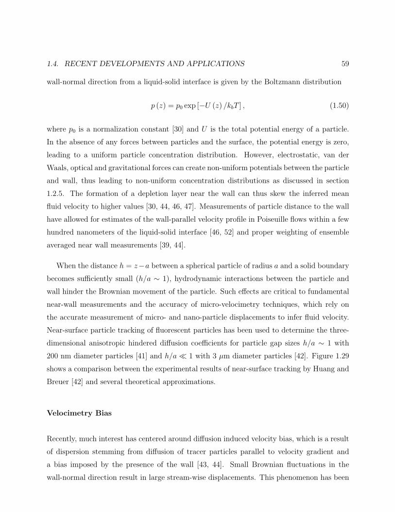
1.4. RECENT DEVELOPMENTS AND APPLICATIONS 59
wall-normal direction from a liquid-solid interface is given by the Boltzmann distribution
p (z) = p0 exp [−U (z) /kbT ] , (1.50)
where p0 is a normalization constant [30] and U is the total potential energy of a particle.
In the absence of any forces between particles and the surface, the potential energy is zero,
leading to a uniform particle concentration distribution. However, electrostatic, van der
Waals, optical and gravitational forces can create non-uniform potentials between the particle
and wall, thus leading to non-uniform concentration distributions as discussed in section
1.2.5. The formation of a depletion layer near the wall can thus skew the inferred mean
fluid velocity to higher values [30, 44, 46, 47]. Measurements of particle distance to the wall
have allowed for estimates of the wall-parallel velocity profile in Poiseuille flows within a few
hundred nanometers of the liquid-solid interface [46, 52] and proper weighting of ensemble
averaged near wall measurements [39, 44].
When the distance h = z−a between a spherical particle of radius a and a solid boundary
becomes sufficiently small (h/a ∼ 1), hydrodynamic interactions between the particle and
wall hinder the Brownian movement of the particle. Such effects are critical to fundamental
near-wall measurements and the accuracy of micro-velocimetry techniques, which rely on
the accurate measurement of micro- and nano-particle displacements to infer fluid velocity.
Near-surface particle tracking of fluorescent particles has been used to determine the three-
dimensional anisotropic hindered diffusion coefficients for particle gap sizes h/a ∼ 1 with
200 nm diameter particles [41] and h/a 1 with 3 µm diameter particles [42]. Figure 1.29
shows a comparison between the experimental results of near-surface tracking by Huang and
Breuer [42] and several theoretical approximations.
Velocimetry Bias
Recently, much interest has centered around diffusion induced velocity bias, which is a result
of dispersion stemming from diffusion of tracer particles parallel to velocity gradient and
a bias imposed by the presence of the wall [43, 44]. Small Brownian fluctuations in the
wall-normal direction result in large stream-wise displacements. This phenomenon has been
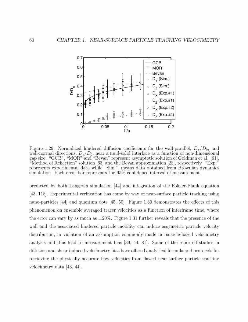
60 CHAPTER 1. NEAR-SURFACE PARTICLE TRACKING VELOCIMETRY
0 0.05 0.1 0.15 0.20
0.1
0.2
0.3
0.4
0.5
0.6
0.7
h/a
D/D
0
GCBMORBevanD
X (Sim.)
DZ (Sim.)
DX (Exp.#1)
DZ (Exp.#1)
DX (Exp.#2)
DZ (Exp.#2)
Figure 1.29: Normalized hindered diffusion coefficients for the wall-parallel, Dx/D0, andwall-normal directions, Dz/D0, near a fluid-solid interface as a function of non-dimensionalgap size. “GCB”, “MOR” and “Bevan” represent asymptotic solution of Goldman et al. [61],“Method of Reflection” solution [63] and the Bevan approximation [28], respectively. “Exp.”represents experimental data while “Sim.” means data obtained from Brownian dynamicssimulation. Each error bar represents the 95% confidence interval of measurement.
predicted by both Langevin simulation [44] and integration of the Fokker-Plank equation
[43, 118]. Experimental verification has come by way of near-surface particle tracking using
nano-particles [44] and quantum dots [45, 50]. Figure 1.30 demonstrates the effects of this
phenomenon on ensemble averaged tracer velocities as a function of interframe time, where
the error can vary by as much as ±20%. Figure 1.31 further reveals that the presence of the
wall and the associated hindered particle mobility can induce assymetric particle velocity
distribution, in violation of an assumption commonly made in particle-based velocimetry
analysis and thus lead to measurement bias [39, 44, 81]. Some of the reported studies in
diffusion and shear induced velocimetry bias have offered analytical formula and protocols for
retrieving the physically accurate flow velocities from flawed near-surface particle tracking
velocimetry data [43, 44].
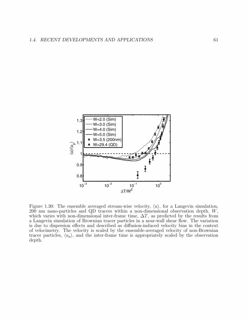
1.4. RECENT DEVELOPMENTS AND APPLICATIONS 61
10−3
10−2
10−1
100
0.8
0.9
1
1.1
1.2
1.3
ΔT/W2
⟨u⟩/⟨
u p⟩
W=2.0 (Sim)W=3.0 (Sim)W=4.0 (Sim)W=5.0 (Sim)W=3.5 (200nm)W=29.4 (QD)
Figure 1.30: The ensemble averaged stream-wise velocity, 〈u〉, for a Langevin simulation,200 nm nano-particles and QD tracers within a non-dimensional observation depth, W ,which varies with non-dimensional inter-frame time, ∆T , as predicted by the results froma Langevin simulation of Brownian tracer particles in a near-wall shear flow. The variationis due to dispersion effects and described as diffusion-induced velocity bias in the contextof velocimetry. The velocity is scaled by the ensemble-averaged velocity of non-Browniantracer particles, 〈up〉, and the inter-frame time is appropriately scaled by the observationdepth.
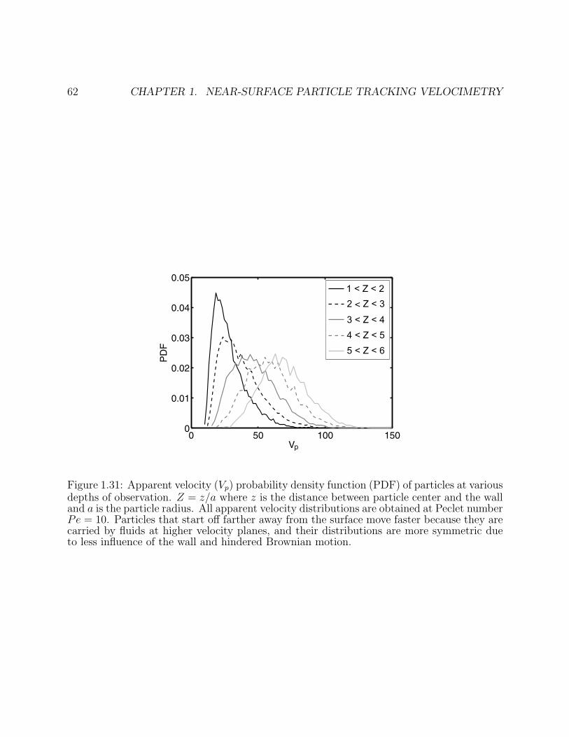
62 CHAPTER 1. NEAR-SURFACE PARTICLE TRACKING VELOCIMETRY
0 50 100 1500
0.01
0.02
0.03
0.04
0.05
V
PD
F
1 < Z < 22 < Z < 3
3 < Z < 44 < Z < 55 < Z < 6
p
Figure 1.31: Apparent velocity (Vp) probability density function (PDF) of particles at variousdepths of observation. Z = z/a where z is the distance between particle center and the walland a is the particle radius. All apparent velocity distributions are obtained at Peclet numberPe = 10. Particles that start off farther away from the surface move faster because they arecarried by fluids at higher velocity planes, and their distributions are more symmetric dueto less influence of the wall and hindered Brownian motion.
1.5. CONCLUSION 63
1.5 Conclusion
In this chapter, we have tried not only to outline the basic concepts and underlying physics
associated with near wall particle tracking velocimetry using total internal reflection floures-
cence (TIRF) microscopy, but also to highlight the practical issues associated with the design,
assembly and operation of a TIRF velocimetry system for micro- and nano-scale fluid mea-
surements. As is often the case with new diagnostic methods, the first few experiments
reported are exciting, but often only suggestive - they reveal the promise of a new technique,
but expose more questions than they provide answers. This pattern has certainly been true in
the history of near wall velocimetry. However, in the past decade the technique has matured
considerably and many, certainly not all, of these questions have been identified and in some
cases answered. As of today, many of the issues associated with the operation of a TIRF
velocimetry system and the analysis of the resultant data have been optimized, algorithms
have been developed to track particles, and many of the issues that make interpretation
difficult have been identified and explained, so as to make TIRF microscopy a useful and
quantitative approach for practical microfluidic measurements.
To be sure, many challenges still remain to be addressed. Accurate determination of the
wall-normal position of tracer particles remains difficult, and is hindered by the difficulty in
discriminating between particle size variations and the position of the particle in the evanes-
cent field. This will improve as particle manufacturing techniques improve, and with the
adoption of even more advanced optical methods that employ, for example, interferometry,
or other phase- and polarization sensitive methods. Another challenge is the ability to iden-
tify and track ensembles of particles whose thermal motions may be orders of magnitude
larger than the local fluid velocity. This will become easier as imaging systems continue
to improve, and with the further development of statistical methods for extracting particle
displacements. Lastly, the physics of near-wall flows, and of the motion of particles in prox-
imity to the liquid-solid interface are extraordinarily subtle, and these complexities continue
to generate results that are often unexpected and require explanation. These explanations
will take time as we continue to sort out the relative roles of each force and phenomenon
before we arrive at a unified understanding of near wall fluidic flows.
64 CHAPTER 1. NEAR-SURFACE PARTICLE TRACKING VELOCIMETRY

Bibliography
[1] Adam Bange, H. Brian Halsall, and William R. Heineman. Microfluidic immunosensorsystems. Biosensors and Bioelectronics, 20:2488–2503, 2005.
[2] Samuel K. Sia and George M. Whitesides. Microfluidic devices fabricated inpoly(dimethylsiloxane) for biological studies. Electrophoresis, 24:3563–3576, 2003.
[3] Jan Kruger, Kirat Singh, Alan O’neill, Carl Jackson, Alan Morrison, and Peter O’Brien.Development of a microfluidic device for fluorescence activated cell sorting. Journal ofMicromechanics and Microengineering, 12:486–494, 2002.
[4] W. Mark Saltzman and William L. Olbricht. Building drug delivery into tissue engi-neering. Nature Reviews, 1:177–186, 2002.
[5] Terry P. Bigioni, Xiao-Min Lin, Toan T. Nguyen, Eric I. Corwin, Thomas A. Witten,and Heinrich M. Jaeger. Kinetically driven self assembly of highly ordered nanoparti-clemonolayers. Nature Materials, 5:265–270, 2005.
[6] O V Salata. Applications of nanoparticles in biology and medicine. Journal ofNanobiotechnology, 2, 2004.
[7] David J. Beebe, Glennys A. Mensing, and Glenn M. Walker. Physics and applicationsof microfluidics in biology. Annual Review of Biomedical Engineering, 4:261–286, 2002.
[8] K. Johan A. Westin, Kenneth S. Breuer, Chang-Hwan Choi, Peter Huang, ZhiqiangCao, Bruce Caswell, Peter D. Richardson, and Merwin Sibulkin. Liquid transportproperties in sub-micron channel flows. In Proceedings of 2001 ASME InternationalMechanical Engineering Congress and Exposition, 2001.
[9] George E. Karniadakis and Ali Beskok. Micro flows: fundamentals and simulation.Springer, 2002.
[10] Eric Lauga, Michael P. Brenner, and Howard A. Stone. Microfluidics: The no-slipboundary condition. In J. Foss anc C. Tropea and A. Yarin, editors, Handbook ofExperimental Fluid Dynamics, chapter 19. Springer, New York, 2007.
[11] Bin Zhao, Jeffrey S. Moore, and David J. Beebe. Surface-directed liquid flow insidemicrochannels. Science, 291:1023–1026, 2001.
[12] Bin Zhao, Jeffrey S. Moore, and David J. Beebe. Principles of surface-directed liquidflow in microfluidic channels. Analytical Chemistry, 74:4259–4268, 2002.
[13] Zbigniew Adamczyk, Katarzyna Jaszczolt, Barbara Siwek, and Pawel Weronski. Irre-versible adsorption of particles at random-site surfaces. Journal of Chemical Physics,120:11155–11162, 2004.
65
66 BIBLIOGRAPHY
[14] Kai-Chien Chang and Daniel A. Hammer. Influence of direction and type of appliedforce on the detachment of macromolecularly-bound particles from surfaces. Langmuir,12:2271–2282, 1996.
[15] M. Chaoui and F. Feuillebois. Creeping flow around a sphere in a shear flow close toa wall. Quarterly Journal of Mechanics and Applied Mathematics, 56:381–410, 2003.
[16] Poppo J. Wit, Albert Poortinga, Jaap Noordmans, Henry C. van der Mei, and Henk J.Busscher. Deposition of polystyrene particles in a parallel plate flow chamber underattractive and repulsive electrostatic conditions. Langmuir, 15:2620–2626, 1999.
[17] P. J. A. Hartman Kok, S. G. Kazarian, B. J. Briscoe, and C. J. Lawrence. Effects ofparticle size on near-wall depletion in mono-dispersed colloidal suspensions. Journalof Colloid and Interface Science, 280:511–517, 2004.
[18] Daniel Axelrod. Total internal reflection fluorescence microscopy. In Methods in CellBiology, volume 30, chapter 9, pages 245–270. Academic Press, Inc., 1989.
[19] Roshdi Rashed. A pioneer in anaclastics: Ibn Sahl on burning mirros and lenses. Isis,81:464–491, 1990.
[20] Chris Rowe Tiatt, George P. Anderson, and Frances S. Ligler. Evanescent wave fluo-rescence biosensors. Biosensors and Bioelectronics, 20:2470–2487, 2005.
[21] Daniel Axelrod. Total internal reflection fluorescence microscopy in cell biology. Traffic,2:764–774, 2001.
[22] Daniel Axelrod, Thomas P. Burghardt, and Nancy T. Thompson. Total internal re-flection fluorescence. Annual Review of Biophysics and Bioengineering, 13:247–268,1984.
[23] N. L. Thompson and B. C. Langerholm. Total internal reflection fluorescence: appli-cations in cellular biophysics. Current Opinion in Biotechnology, 8:58–64, 1997.
[24] Derek Toomre and Dietmar J. Manstein. Lighting up the cell surface with evanescentwave microscopy. Trends in Cell Biology, 11:298–303, 2001.
[25] H. H. von Grunberg, L. Helden, P. Leiderer, and C. Bechinger. Measurement of sur-face charge densities on brownian particles using total internal reflection microscopy.Journal of Chemical Physics, 114:10094–10104, 2001.
[26] Scott G. Flicker, Jennifer L. Tipa, and Stacy G. Bike. Quantifying double-layer re-pulsion between a colloidal sphere and a glass plate using total internal reflectionmicroscopy. Journal of Colloid and Interface Science, 158:317–325, 1993.
[27] Stacy G Bike. Measureing colloidal forces using evanescent wave scattering. Colloidand Interface Science, 5:144–150, 2000.
[28] Michael A. Bevan and Dennis C. Prieve. Hindered diffusion of colloidal particles verynear to a wall: revisited. Journal of Chemical Physics, 113:1228–1236, 2000.
[29] Robert Kun and Janos H. Fendler. Use of attenuated total internal reflection-fouriertransform infrared spectroscopy to investigate the adsorption of and interactions be-tween charged latex particles. Journal of Physical Chemistry, 108:3462–3468, 2004.
[30] Dennis C. Prieve. Measurement of colloidal forces with TIRM. Advances in Colloidand Interface Science, 82:93–125, 1999.
BIBLIOGRAPHY 67
[31] Dennis C Prieve and Nassar A Frej. Total internal reflection microscopy: a tool formeasuring colloidal forces. Langmuir, 6:396–403, 1990.
[32] Dennis C. Prieve and John Y. Walz. Scattering of an evanescent surface wave by amicroscopic dielectric sphere. Applied Optics, 32:1629–1641, 1993.
[33] P. Buchhave. Particle image velocimetry. In Lars Lading, Graham Wigley, and PrebenBuchhave, editors, Optical diagnostics for flow processes, pages 247–270. Plenum Press,New York, 1994.
[34] S. T. Wereley and C. D. Meinhart. Micron-resolution particle image velocimetry. InK. Breuer, editor, Microscale Diagnostic Techniques, pages 51–112. Springer, 2005.
[35] C. M. Zettner and M. Yoda. Particle velocity field measurements in a near-wall flowusing evanescent wave illumination. Experiments in Fluids, 34:115–121, 2003.
[36] S. Jin, P. Huang, J. Park, J. Y. Yoo, and K. S. Breuer. Near-surface velocimetry usingevanescent wave illumination. Experiments in Fluids, 37:825–833, 2004.
[37] Haifeng Li, Reza Sadr, and Minami Yoda. Multilayer nano-particle image velocimetry.Experiments in Fluids, 41:185–194, 2006.
[38] Reza Sadr, Minami Yoda, Z. Zheng, and A. T. Conlisk. An experimental studyof electro-osmotic flow in rectangular microchannels. Journal of Fluid Mechanics,506:357–367, 2004.
[39] Peter Huang, Jeffrey S. Guasto, and Kenneth S. Breuer. Direct measurement of slipvelocities using three-dimensional total internal reflection velocimetry. Journal of FluidMechanics, 566:447–464, 2006.
[40] Peter Huang and Kenneth S. Breuer. Direct measurement of slip length in electrolytesolutions. Physics of Fluids, 19:028104, 2007.
[41] K. D. Kihm, A. Banerjee, C. K. Choi, and T. Takagi. Near-wall hindered brown-ian diffusion of nanoparticles examined by three-dimensional ratiometric total internalreflection fluorescence microscopy (3-d r-tirfm). Experiments in Fluids, 37:811–824,2004.
[42] Peter Huang and Kenneth S. Breuer. Direct measurement of anisotropic near-wall hin-dered diffusion using total internal reflection velocimetry. Physical Review E, 76:046307,2007.
[43] Reza Sadr, Christel Hohenegger, Haifeng Li, Peter J. Mucha, and Minami Yoda.Diffusion-induced bias in near-wall velocimetry. Journal of Fluid Mechanics, 577:443–456, 2007.
[44] Peter Huang, Jeffrey S. Guasto, and Kenneth S. Breuer. The effects of hinderedmobility and depletion of particles in near-wall shear flows and the implications fornano-velocimetry. Journal of Fluid Mechanics, In Press, 2009.
[45] Shahram Pouya, Manoochehr M. Koochesfahani, Andrew B. Greytak, Moungi G.Bawendi, and Daniel Nocera. Experimental evidence of diffusion-induced bias in near-wall velocimetry using quantum dot measurements. Experiments in Fluids, 44:1035–1038, 2008.
[46] Haifeng Li and Minami Yoda. Multilayer nano-particle image velocimetry (MnPIV) inmicroscale Poiseuille flows. Measurement Sciecne and Technology, 19:075402, 2008.
68 BIBLIOGRAPHY
[47] Jeffrey S. Guasto. Micro- and Nano-scale Colloidal Dynamics Near Surfaces. PhDthesis, Brown University, 2008.
[48] Shahram Pouya, Manoochehr Koochesfahani, Preston Snee, Moungi Bawendi, andDaniel Nocera. Single quantum dot (qd) imaging of fluid flow near surfaces. Experi-ments in Fluids, 39:784–786, 2005.
[49] Jeffrey S. Guasto, Peter Huang, and Kenneth S. Breuer. Statistical particle trackingvelocimetry using molecular and quantum dot tracer particles. Experiments in Fluids,2006. in press.
[50] Jeffrey S. Guasto and Kenneth S. Breuer. High-speed quantum dot tracking andvelocitmetry using evanesent wave illumination. Experiments in Fluids, In Press, 2009.
[51] Jeffrey S Guasto and Kenneth S Breuer. Simultaneous, ensemble-averaged measure-ment of near-wall temperature and velocity in steady micro-flows using single quantumdot tracking. Experiments in Fluids, 45:157–166, 2008.
[52] D Lasne, A Maali, Y Amarouchene, L Cognet, B Lounis, and H Kellay. Velocity profilesof water flowing past solid glass surfaces using fluorescent nanoparticles and moleculesas velocity probes. Physical Review Letters, 100:214502, 2008.
[53] S.O. Kasap. Optoelectronics and Photonics: Principles and Practices, chapter 1, pages1–49. Prentice Hall, 2001.
[54] H Chew. Radiation and lifetimes of atoms inside dielectri partilces. Physical ReviewA, 38:3410–3416, 1988.
[55] H Chew, P J McNulty, and M Kerker. Model for Raman and fluorescent scattering bymolecule embedded in small particles. Physical Review A, 13:396–404, 1976.
[56] Robert Brown. A brief account of microscopical observations made in the months ofjune, july and august, 1827, on the particles contained in the pollen of plants; and onthe general existence of active molecules in organic and inorganic bodies. PhilosophicalMagazine, 4:161–173, 1828.
[57] Albert Einstein. ber die von der molekularkinetischen theorie der wrme gefordertebewegung von in ruhenden flssigkeiten suspendierten teilchen. Annalen der Physik,17:549–560, 1905.
[58] E L Cussler. Diffusion: Mass Transfer in Fluid Systems. Cambridge University Press,1997.
[59] Donald A McQuarrie. Statistical Mechanics, chapter 17, pages 379–401. UniversityScience Books, 2000.
[60] Howard Brenner. The slow motion of a sphere through a viscous fluid towards a planewall. Chemical Engineering Science, 16:242–251, 1961.
[61] A. J. Goldman, R. G. Cox, and H. Brenner. Slow viscous motion of a sphere parallelto a plane wall - I: motion through a quiescent fluid. Chemical Engineering Science,22:637–651, 1967.
[62] A. J. Goldman, R. G. Cox, and H. Brenner. Slow viscous motion of a sphere parallelto a plane wall - II: Couette flow. Chemical Engineering Science, 22:653–660, 1967.
[63] John Happel and Howard Brenner. Low Reynolds Number Hydrodynamics: With Spe-cial Applications to Particulate Media. Springer, 1983.
BIBLIOGRAPHY 69
[64] Nasser A. Frej and Dennis C. Prieve. Hindered diffusion of a single sphere very near awall in a nonuniform force field. Journal of Chemical Physics, 98:7552–7564, 1993.
[65] Binhua Lin, Jonathan Yu, and Stuart A. Rice. Direct measurements of constrainedbrownian motion of an isolated sphere between two walls. Physical Review E, 62:3909–3919, 2000.
[66] Ratna J. Oetama and John Y. Walz. Simultaneous investigation of sedimentation anddiffusion of a single colloidal particle near an interfce. The Journal of Chemical Physics,124:164713, 2006.
[67] Arindam Banerjee and Kenneth D. Kihm. Experimental verification of near-wall hin-dered diffusion for the brownian motion of nanoparticles using evanescent wave mi-croscopy. Physical Review E, 72:042101, 2005.
[68] William M Dean. Analysis of Transport Phenomena. Oxford University Press, 1998.
[69] Anne Pierres, Anne-Marie Benoliel, Cheng Zhu, and Pierre Bongrand. Diffusion ofmicrospheres in shear flow near a wall: use to measure binding rates between attachedmolecules. Biophysical Journal, 81:25–42, 2001.
[70] Michael R. King and David T. Leighton Jr. Measurement of the inertial lift on a movingsphere in contact with a plane wall in a shear flow. Physics of Fluids, 9:1248–1255,1997.
[71] Pradeep Cherukat and John B. McLaughlin. The inertial lift on a rigid sphere in alinear shear flow field near a flat wall. Journal of Fluid Mechanics, 263:1–18, 1994.
[72] R A L Jones. Soft Condensed Matter. Oxford University Press, 2004.
[73] Matthew R. Oberholzer, Norman J. Wagner, and Abraham M. Lenhoff. Grand canoni-cal Brownian dynamics simulation of colloidal adsorption. Journal of Chemical Physics,107:9157–9167, 1997.
[74] J N Israelachvili and D Tabor. The measurement of van der Waals dispersion forcesin the range 1.5 to 130 nm. Proceeding of the Royal Society of London A, 331:19–38,1972.
[75] H. C. Hamaker. The Londonvan der Waals attraction between spherical particles.Physica (Amsterdam), 4:1058–1072, 1937.
[76] V Adrian Parsegian. Van Der Waals Forces: A Handbook for Biologists, Chemists,Engineers and Physicists. Cambridge University Press, 2006.
[77] A Ashkin, J M Dziedzic, J E Bjorkholm, and S Chu. Observation of a single-beamgradient force optical trap for dielectric particles. Optics Letters, 11:288–290, 1986.
[78] Lukas Novotny and Bert Hecht. Principles of Nano-Optics. Cambridge UniversityPress, 2006.
[79] M Doi and S F Edwards. The Theory of Polymer Dynamics, chapter 2, pages 46–50.Oxford University Press, 1986.
[80] Shiya Inoue and Kenneth R. Spring. Video Microscopy: The Fundamentals. PlenumPress, second edition, 1997.
[81] Peter Huang. Near-surface slip flow and hindered colloidal diffusion at the nano-scale.PhD thesis, Brown University, 2006.
70 BIBLIOGRAPHY
[82] S Zhu, A W Yu, D Hawley, and R Roy. Frustrated total internal reflection: a demon-stration and review. American Journal of Physics, 57:601–607, 1986.
[83] J. G. Santiago, S. T. Wereley, C. D. Meinhart, D. J. Beebe, and R. J. Adrian. A particleimage velocimetry system for microfluidics. Experiments in Fluids, 25:316–319, 1998.
[84] J. C. Crocker and D. G. Grier. When like charges attract: The effects of geometricalconfinement on long-range colloidal interactions. Physical Review Letters, 77:1897–1900, 1996.
[85] Michael K. Cheezum, William F. Walker, and William H. Guilford. Quantitativecomparison of algorithms for tracking single fluorescent particles. Biophysical Journal,81:2378–2388, 2001.
[86] Victor Breedveld, Dirk van den Ende, and Anubhav Tripathi Anreas Acrivos. Themeasurement of the shear-induced particle and fluid tracer diffusivities in concentratedsuspensions by a novel method. Journal of Fluid Mechanics, 375:297–318, 1998.
[87] Nicholas T Ouellette, Haitao Xu, and Eberhard Bodenschatz. A quantitative studyof three-dimensional lagrangian particle tracking algorithms. Experiments in Fluids,40:301–313, 2006.
[88] Hannes Schniepp and Vahid Sandoghdar. Spontaneous emission of europium ionsembedded in deielectric nanospheres. Physicsl Review Letters, 89:257403, 2002.
[89] Brian J Schmidt, Peter Huang, Kenneth S Breuer, and Michael B Lawrence. Catchstrip assay for the relative assessment of two-dimensional protein association kinetics.Analytical Chemistry, 80:944–950, 2008.
[90] Phillipe Robert, Anne-Marie Benoliel, and Pierre Bondgrand. What is the biologicalrelevance of the specific bond properties revealed by single-molecule studies? Journalof Molecular Recognition, 20:432–447, 2007.
[91] Marcel Bruchez, Mario Moronne, Peter Gin, Shimon Weiss, and A. Paul Alivisatos.Semiconductor nanocrystals as fluorescent biological labels. Science, 281:2013–2016,1998.
[92] M. Nirmal, B. O. Dabbousi, M. G. Bawendi, J. J. Macklin, J. K. Trautman, T. D. Har-ris, and L. E. Brus. Fluorescence intermittency in single cadmium selenide nanocrystals.Nature, 383:802–804, 1996.
[93] Patrick E Freudenthal, Matt Pommer, Carl D Meinhart, and Brian D Piorek. Quantumnanospheres for sub-micron particle image velocimetry. Experiments in Fluids, 43:525–543, 2007.
[94] Ronald J. Adrian. Particle imaging techniques for experimental fluid mechanics. An-nual Review of Fluid Mechanics, 23:261–304, 1991.
[95] J C Crocker and D G Grier. Methods of digital video microscopy for colloidal studies.Journal of Colloid and Interface Science, 179:298–310, 1996.
[96] C.I. Bouzigues, P. Tabeling, and L. Bocquet. Nanofluidics in the debye layer at hy-drophilic and hydrophobic surfaces. Physical Review Letters, 101:114503, 2008.
[97] Chang-Hwan Choi, Johan A. Westin, and Kenneth S. Breuer. Apparent slip flows inhydrophilic and hydrophobic microchannels. Physics of Fluids, 15:2897–2902, 2003.
BIBLIOGRAPHY 71
[98] YingXi Zhu and Steve Granick. Limites of the hydrodynamic no-slip boundary condi-tion. Physical Review Letters, 88:106102, 2002.
[99] C. Neto, V. S. J. Craig, and D. R. M. Williams. Evidence of shear-dependent boundaryslip in newtonian liquids. The European Physical Journal E, 12:S71–S74, 2003.
[100] C. Cottin-Bizonne, B. Cross, A. Steinberger, and E. Charlaiz. Boundary slip on smoothhydrophobic surfaces: intrinsic effects and possible artifacts. Physical Review Letters,94:056102, 2005.
[101] R. Pit, H. Hervet, and L. Leger. Direct experimental evidence of slip in hexadecane:solid interface. Physical Review Letters, 85:980–983, 2000.
[102] Derek C. Tretheway and Carl D. Meinhart. Apparent fluid slip at hydrophobic mi-crochannel walls. Physics of Fluids, 14:L9–L12, 2002.
[103] Pierre Joseph and Patrick Tabeling. Direct measurement of the apparent slip length.Physical Review E, 71:035303(R), 2005.
[104] D. Lumma, A. Best, A. Gansen, F. Feuillebois, J. O. Radler, and O. I. Vinogradova.Flow profile near a wall measured by double-focus fluorescence cross-correlation. Phys-ical Review E, 67:056313, 2003.
[105] Peter A. Thompson and Sandra M. Troian. A general boundary condition for liquidflow at solid surfaces. Nature, 389:360–362, 1997.
[106] Jean-Louis Barrat and Lyderic Bocquet. Large slip effect at a nonwetting fluid-solidinterface. Physical Review Letters, 82:4671–4674, 1999.
[107] Marek Cieplak, Joel Koplik, and Jayanth R. Banavar. Boundary conditions at a fluid-solid surface. Physical Review Letters, 86:803–806, 2001.
[108] T. M. Galea and Phil Attard. Molecular dynamics study of the effect of atomicroughness on the slip length at the fluid-solid boundary during shear flow. Langmuir,20:3477–3482, 2004.
[109] Gyoko Nagayama and Ping Cheng. Effects of interface wettability on microscale flowby molecular dynamics simulation. International Journal of Heat and Mass Transfer,47:501–513, 2004.
[110] Cecile Cottin-Bizonne, Jean-Louis Barrat, Lyderic Bocquet, and Elisabeth Charlaiz.Low-friction flows of liquid at nanopattened interfaces. Nature Materials, 2:237–240,2005.
[111] Jian Liu, Markus Enzelberger, and Stephen Quake. A nanoliter rotary device forpolymerase chain reaction. Electrophoresis, 23:1531–1536, 2002.
[112] John R. Thome. Boiling in microchannels: a review of experiment and theory. Inter-national Journal of Heat and Fluid Flow, 25:128–139, 2004.
[113] David Ross, Michal Gaitan, and Laurie E. Locascio. Temperature measurement in mi-crofluidic systems using a temperature-dependent fluorescence dye. Analytical Chem-istry, 73:4117–4123, 2001.
[114] H.J. Kim, K.D. Kihm, and J.S. Allen. Examination of ratiometric laser induced flu-orescence thermometry for microscale spatial measurement resolution. InternationalJournal of Heat and Mass Transfer, 46:3967–3974, 2003.
72 BIBLIOGRAPHY
[115] M.G. Olsen and R.J. Adrian. Brownian motion and correlation in particle imagevelocimetry. Optics and Laser Technology, 32:621–627, 2000.
[116] Tian-Cai Liu, Zhen-Li Huang, Hai-Qiao Wang, Jian-Hao Wang, Xiu-Qing Li, Yuan-DiZhao, and Qing ming Luo. Temperature-dependent photluminescence of water-solublequantum dots for a bioprobe. Analytica Chimica Acta, 559:120–123, 2006.
[117] A. R. Bausch and D. A. Weitz. Tracking the dynamics of single quantum dots: Beatingthe optical resolution twice. Journal of Nanoparticle Research, 4:477–481, 2002.
[118] Reza Sadr, Haifeng Li, and Minami Yoda. Impact of hindered brownian diffusion onthe accuracy of particle-image velocimetry using evanescent-wave illumination. Exper-iments in Fluids, 38:90–98, 2005.