near-horizon geometry and warped conformal … geometry and warped conformal symmetry ... do with...
TRANSCRIPT
TUW–15–22
Near-Horizon Geometry and Warped Conformal Symmetry
Hamid Afshar∗†, Stephane Detournay‡, Daniel Grumiller§ and Blagoje Oblak‡¶
∗Van Swinderen Institute for Particle Physics and Gravity, University of Groningen
Nijenborgh 4, 9747 AG Groningen, The Netherlands
† School of Physics, Institute for Research in Fundamental Sciences (IPM)
P.O.Box 19395-5531, Tehran, Iran
‡Physique Theorique et Mathematique, Universite Libre de Bruxelles and International Solvay Institutes
Campus Plaine C.P. 231, B-1050 Bruxelles, Belgium
§Institute for Theoretical Physics, TU Wien
Wiedner Hauptstrasse 8-10/136, A-1040 Vienna, Austria
¶DAMTP, Centre for Mathematical Sciences, University of Cambridge
Wilberforce Road, Cambridge CB3 0WA, United Kingdom
E-mail: [email protected], [email protected],
[email protected], [email protected]
Abstract
We provide boundary conditions for three-dimensional gravity including boosted Rind-
ler spacetimes, representing the near-horizon geometry of non-extremal black holes or flat
space cosmologies. These boundary conditions force us to make some unusual choices, like
integrating the canonical boundary currents over retarded time and periodically identifying
the latter. The asymptotic symmetry algebra turns out to be a Witt algebra plus a twisted
u(1) current algebra with vanishing level, corresponding to a twisted warped CFT that
is qualitatively different from the ones studied so far in the literature. We show that
this symmetry algebra is related to BMS by a twisted Sugawara construction and exhibit
relevant features of our theory, including matching micro- and macroscopic calculations of
the entropy of zero-mode solutions. We confirm this match in a generalization to boosted
Rindler-AdS. Finally, we show how Rindler entropy emerges in a suitable limit.
arX
iv:1
512.
0823
3v2
[he
p-th
] 2
0 Ja
n 20
16

Contents
1 Introduction 1
2 Boosted Rindler boundary conditions 3
2.1 Boundary conditions . . . . . . . . . . . . . . . . . . . . . . . . . . . . . . . 4
2.2 Variational principle . . . . . . . . . . . . . . . . . . . . . . . . . . . . . . . 5
2.3 Asymptotic symmetry transformations . . . . . . . . . . . . . . . . . . . . . 6
3 Asymptotic symmetry group 8
3.1 An empty theory . . . . . . . . . . . . . . . . . . . . . . . . . . . . . . . . . 8
3.2 Quasi-Rindler currents and charges . . . . . . . . . . . . . . . . . . . . . . . 10
3.3 Warped Virasoro group and coadjoint representation . . . . . . . . . . . . . 12
4 Quasi-Rindler thermodynamics 14
4.1 Modular invariance and microscopic entropy . . . . . . . . . . . . . . . . . . 14
4.2 Boosted Rindler spacetimes and their Killing vectors . . . . . . . . . . . . . 16
4.3 Euclidean boosted Rindler . . . . . . . . . . . . . . . . . . . . . . . . . . . . 18
4.4 Macroscopic free energy and entropy . . . . . . . . . . . . . . . . . . . . . . 20
5 Boosted Rindler-AdS 20
5.1 Boundary conditions and symmetry algebra . . . . . . . . . . . . . . . . . . 20
5.2 Microscopic quasi-Rindler-AdS entropy . . . . . . . . . . . . . . . . . . . . . 22
5.3 Macroscopic quasi-Rindler-AdS entropy . . . . . . . . . . . . . . . . . . . . 23
6 Rindlerwahnsinn? 24
6.1 Retarded choices? . . . . . . . . . . . . . . . . . . . . . . . . . . . . . . . . . 24
6.2 Rindler entropy? . . . . . . . . . . . . . . . . . . . . . . . . . . . . . . . . . 25
6.3 Other approaches . . . . . . . . . . . . . . . . . . . . . . . . . . . . . . . . . 26
A On representations of the warped Virasoro group 27
A.1 Coadjoint representation . . . . . . . . . . . . . . . . . . . . . . . . . . . . . 27
A.2 Induced representations . . . . . . . . . . . . . . . . . . . . . . . . . . . . . 31
B Rindler thermodynamics 35
B.1 Rindler horizon and temperature . . . . . . . . . . . . . . . . . . . . . . . . 35
B.2 Rindler free energy . . . . . . . . . . . . . . . . . . . . . . . . . . . . . . . . 36
B.3 Rindler entropy . . . . . . . . . . . . . . . . . . . . . . . . . . . . . . . . . . 37
References 37
1 Introduction
Rindler space arises generically as the near horizon approximation of non-extremal black
holes or cosmological spacetimes. Thus, if one could establish Rindler holography one may
expect it to apply universally. In particular, obtaining a microscopic understanding of
Rindler entropy could pave the way towards some of the unresolved puzzles in microscopic
state counting, like a detailed understanding of the entropy of the Schwarzschild black hole,
which classically is one of the simplest black holes we know, but quantum-mechanically
seems to be among the most complicated ones.
Our paper is motivated by this line of thought, but as we shall see the assumptions
we are going to impose turn out to have a life of their own and will take us in somewhat
unexpected directions. This is why we will label what we do in this work as “quasi-Rindler
holography” instead of “Rindler holography”.
Three-dimensional gravity
For technical reasons we consider Einstein gravity in three spacetime dimensions [1]. While
simpler than its higher-dimensional relatives, it is still complex enough to exhibit many
of the interesting features of gravity: black holes [2], cosmological spacetimes [3] and
boundary gravitons [4].
In the presence of a negative cosmological constant the seminal paper by Brown and
Henneaux [4] established one of the precursors of the AdS/CFT correspondence. The key
ingredient to their discovery that AdS3 Einstein gravity must be dual to a CFT2 was the
imposition of precise (asymptotically AdS) boundary conditions. This led to the realization
that some of the bulk first class constraints become second class at the boundary, so that
boundary states emerge and the physical Hilbert space forms a representation of the 2-
dimensional conformal algebra with specific values for the central charges determined by
the gravitational theory.
As it turned out, the Brown–Henneaux boundary conditions can be modified, in the
presence of matter [5], in the presence of higher derivative interactions [6] and even in
pure Einstein gravity [7]. In the present work we shall be concerned with a new type
of boundary conditions for 3-dimensional Einstein gravity without cosmological constant.
Let us therefore review some features of flat space Einstein gravity.
In the absence of a cosmological constant Barnich and Compere pioneered a Brown–
Henneaux type of analysis of asymptotically flat boundary conditions [8] and found a
specific central extension of the BMS3 algebra [9], which is isomorphic to the Galilean
conformal algebra [10–12]. Based on this, there were numerous developments in the past
few years, like the flat space chiral gravity proposal [13], the counting of flat space cos-
mology microstates [14], the existence of phase transitions between flat space cosmologies
and hot flat space [15, 16], higher spin generalizations of flat space gravity [17], new in-
sights into representations and characters of the BMS3 group [18,19] with applications to
1
the 1-loop partition function [20], flat space holographic entanglement entropy [21] and
numerous other aspects of flat space holography [22–24].
Quasi-Rindler gravity
As we shall show in this paper, the flat space Einstein equations,
Rµν = 0, (1.1)
do allow for solutions that do not obey the Barnich–Compere boundary conditions but
instead exhibit asymptotically Rindler behavior,
ds2 ∼ O(r) du2 − 2 dudr + dx2 +O(1) dudx+ . . . (1.2)
The main goal of the present work is to set up these boundary conditions, to prove their
consistency and to discuss some of the most relevant consequences for holography, in
particular the asymptotic symmetry algebra and a comparison between macroscopic and
microscopic entropies. Some previous literature on asymptotically Rindler spacetimes is
provided by Refs. [25–32].
Before we delve into the relevant technicalities we address one conceptual issue that
may appear to stop any attempt to Rindler holography in its track. For extremal black
holes the usual near-horizon story works due to their infinite throat, which implies that
one can consistently replace the region near the horizon by the near-horizon geometry
and apply holography to the latter. By contrast, non-extremal black holes do not have an
infinite throat. Therefore, the asymptotic region of Rindler space in general has nothing to
do with the near-horizon region of the original theory. So even if one were to find some dual
field theory in some asymptotic Rindler space, it may not be clear why the corresponding
physical states should be associated with the original black hole or cosmological spacetime.
However, as we shall see explicitly, the notion of a “dual theory living at the boundary” is
misleading; one could equally say that the “field theory lives near the horizon”, since (in
three dimensions) the canonical charges responsible for the emergence of physical boundary
states are independent of the radial coordinate. While we are going to encounter a couple
of obstacles to apply Rindler holography the way we originally intended to do, we do not
consider the finiteness of the throat of non-extremal black holes as one of them.
Starting with the assumption (1.2) we are led to several consequences that we did not
anticipate. The first one is that, on-shell, the functions specifying the spacetime metric
depend on retarded time u instead of the spatial coordinate x, as do the components of the
asymptotic Killing vector fields. As a consequence, canonical charges written as integrals
over x all vanish and the asymptotic symmetries are all pure gauge. However, upon writing
surface charges as integrals over u and taking time to be periodic, the asymptotic symmetry
algebra turns out to describe a warped CFT of a type not encountered before: there is no
Virasoro central charge nor a u(1)-level; instead, there is a non-trivial cocycle in the mixed
2
commutator. Based on these results we determine the entropy microscopically and find
that it does not coincide with the naive Rindler entropy, as a consequence of the different
roles that u and x play in quasi-Rindler, versus Rindler, holography. In the quasi-Rindler
setting, we show that our microscopic result for entropy does match the macroscopic one.
As we shall see, the same matching occurs in our generalization to Rindler-AdS.
In summary, in this paper we describe a novel type of theory with interesting symme-
tries inspired by, but slightly different from, naive expectations of Rindler holography.
This work is organized as follows. In section 2 we state boosted Rindler boundary
conditions and provide a few consistency checks. In section 3 we derive the asymptotic
symmetry algebra with its central extension and discuss some implications for the putative
dual theory. Then, in section 4, we address quasi-Rindler thermodynamics, calculate
free energy and compare macroscopic with microscopic results for entropy, finding exact
agreement between the two. Section 5 is devoted to the generalization of the discussion to
quasi-Rindler AdS. Finally, we conclude in section 6 with some of the unresolved issues.
Along the way, we encounter novel aspects of warped conformal field theories, which
we explore in appendix A. Questions related to standard Rindler thermodynamics are
relegated to appendix B.
2 Boosted Rindler boundary conditions
The 3-dimensional line-element [u, r, x ∈ (−∞,∞)]
ds2 = −2a(u) r du2 − 2 dudr + 2η(u) dudx+ dx2 (2.1)
solves the vacuum Einstein equations (1.1) for all functions a, η that depend solely on the
retarded time u. For vanishing η and constant positive a the line-element (2.1) describes
Rindler space with acceleration a. [This explains why we chose the factor −2 in the first
term in (2.1).] If η does not vanish we have boosted Rindler space. These observations
motivate us to formulate consistent boundary conditions that include all line-elements of
the form (2.1) as allowed classical states.
The gravity bulk action we are going to use is the Einstein–Hilbert action
IEH =k
4π
∫d3x√−g R , k =
1
4GN, (2.2)
which, up to boundary terms, is equivalent to the Chern–Simons action [33]
ICS =k
4π
∫〈A ∧ dA+ 2
3 A ∧A ∧A〉 (2.3)
with an isl(2) connection A and corresponding invariant bilinear form 〈· · · 〉. Explicitly,
the isl(2) generators span the Poincare algebra in three dimensions (n,m = 0,±1),
[Ln, Lm] = (n−m)Ln+m [Ln, Mm] = (n−m)Mn+m [Mn, Mm] = 0 , (2.4)
3
and their pairing with respect to the bilinear form 〈· · · 〉 is
〈L1, M−1〉 = 〈L−1, M1〉 = −2 〈L0, M0〉 = 1 (2.5)
(all bilinears not mentioned here vanish). The connection can be decomposed in compo-
nents as A = A+LL1 + A0
LL0 + A−LL−1 + A+MM1 + A0
MM0 + A−MM−1. In terms of these
components the line-element reads
ds2 = gµν dxµ dxν = −4A+MA
−M + (A0
M )2 . (2.6)
Thus, from a geometric perspective the components AnM correspond to the dreibein and
the components AnL to the (dualized) spin-connection [34,35].
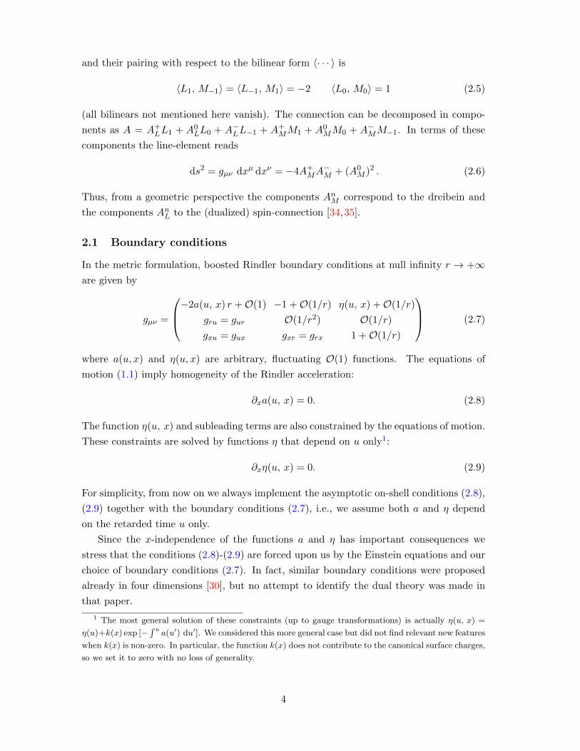
2.1 Boundary conditions
In the metric formulation, boosted Rindler boundary conditions at null infinity r → +∞are given by
gµν =
−2a(u, x) r +O(1) −1 +O(1/r) η(u, x) +O(1/r)
gru = gur O(1/r2) O(1/r)
gxu = gux gxr = grx 1 +O(1/r)
(2.7)
where a(u, x) and η(u, x) are arbitrary, fluctuating O(1) functions. The equations of
motion (1.1) imply homogeneity of the Rindler acceleration:
∂xa(u, x) = 0. (2.8)
The function η(u, x) and subleading terms are also constrained by the equations of motion.
These constraints are solved by functions η that depend on u only1:
∂xη(u, x) = 0. (2.9)
For simplicity, from now on we always implement the asymptotic on-shell conditions (2.8),
(2.9) together with the boundary conditions (2.7), i.e., we assume both a and η depend
on the retarded time u only.
Since the x-independence of the functions a and η has important consequences we
stress that the conditions (2.8)-(2.9) are forced upon us by the Einstein equations and our
choice of boundary conditions (2.7). In fact, similar boundary conditions were proposed
already in four dimensions [30], but no attempt to identify the dual theory was made in
that paper.
1 The most general solution of these constraints (up to gauge transformations) is actually η(u, x) =
η(u)+k(x) exp [−∫ u
a(u′) du′]. We considered this more general case but did not find relevant new features
when k(x) is non-zero. In particular, the function k(x) does not contribute to the canonical surface charges,
so we set it to zero with no loss of generality.
4

For many applications it is useful to recast these boundary conditions in first order
form in terms of an isl(2) connection
A = b−1(
d+a +O(1/r))b, (2.10)
with the ISL(2) group element
b = exp(r2 M−1
)(2.11)
and the auxiliary connection
a+L = 0 a+M = du (2.12a)
a0L = a(u) du a0M = dx (2.12b)
a−L = −12
(η′(u) + a(u)η(u)
)du a−M = −1
2 η(u) dx (2.12c)
where ± refers to L±1 and M±1. Explicitly,
A = a +dr
2M−1 +
a(u)r du
2M−1 (2.13)
where the second term comes from b−1 db and the linear term in r from applying the
Baker–Campbell–Hausdorff formula b−1ab = a − r2 [M−1, a]. Using (2.6), this Chern–
Simons connection is equivalent to the metric (2.1).
2.2 Variational principle
For a well-defined variational principle the first variation of the full action Γ must vanish
for all variations that preserve our boundary conditions (2.7). Since we shall later employ
the Euclidean action to determine the free energy we use Euclidean signature here too.
We make the ansatz2
Γ = − 1
16πGN
∫d3x√g R− α
8πGN
∫d2x√γ K (2.14)
where α is some real parameter. If α = 1, we recover the Gibbons–Hawking–York action
[36]. If α = 12 , we recover an action that is consistent in flat space holography [16]. We
check now which value of α — if any — is consistent for our boosted Rindler boundary
conditions (2.7).
Dropping corner terms, the first variation of the action (2.14) reads on-shell [16]
δΓ∣∣EOM
=1
16πGN
∫d2x√γ(Kij−αKgij+(2α−1)Kninj+(1−α)γijnk∇k
)δgij . (2.15)
2 In the Lorentzian theory the boundary is time-like (space-like) if a is positive (negative). To accom-
modate both signs one should replace K by |K|. To reduce clutter we assume positive a and moreover
restrict to zero mode solutions, a = const., η = const. It can be shown that the variational principle is
satisfied for non-zero mode solutions if it is satisfied for zero mode solutions, as long as ∂xgrx = O(1/r2).
We thank Friedrich Scholler for discussions on the variational principle and for correcting a factor two.
5
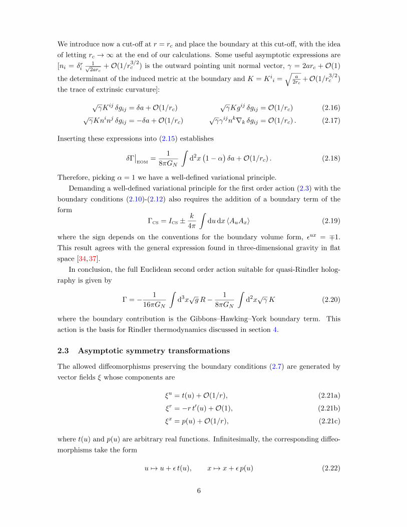
We introduce now a cut-off at r = rc and place the boundary at this cut-off, with the idea
of letting rc →∞ at the end of our calculations. Some useful asymptotic expressions are
[ni = δri1√2arc
+ O(1/r3/2c ) is the outward pointing unit normal vector, γ = 2arc + O(1)
the determinant of the induced metric at the boundary and K = Kii =
√a2rc
+O(1/r3/2c )
the trace of extrinsic curvature]:
√γKij δgij = δa+O(1/rc)
√γKgij δgij = O(1/rc) (2.16)
√γKninj δgij = −δa+O(1/rc)
√γγijnk∇k δgij = O(1/rc) . (2.17)
Inserting these expressions into (2.15) establishes
δΓ∣∣EOM
=1
8πGN
∫d2x
(1− α
)δa+O(1/rc) . (2.18)
Therefore, picking α = 1 we have a well-defined variational principle.
Demanding a well-defined variational principle for the first order action (2.3) with the
boundary conditions (2.10)-(2.12) also requires the addition of a boundary term of the
form
ΓCS = ICS ±k
4π
∫dudx 〈AuAx〉 (2.19)
where the sign depends on the conventions for the boundary volume form, εux = ∓1.
This result agrees with the general expression found in three-dimensional gravity in flat
space [34,37].
In conclusion, the full Euclidean second order action suitable for quasi-Rindler holog-
raphy is given by
Γ = − 1
16πGN
∫d3x√g R− 1
8πGN
∫d2x√γ K (2.20)
where the boundary contribution is the Gibbons–Hawking–York boundary term. This
action is the basis for Rindler thermodynamics discussed in section 4.
2.3 Asymptotic symmetry transformations
The allowed diffeomorphisms preserving the boundary conditions (2.7) are generated by
vector fields ξ whose components are
ξu = t(u) +O(1/r), (2.21a)
ξr = −r t′(u) +O(1), (2.21b)
ξx = p(u) +O(1/r), (2.21c)
where t(u) and p(u) are arbitrary real functions. Infinitesimally, the corresponding diffeo-
morphisms take the form
u 7→ u+ ε t(u), x 7→ x+ ε p(u) (2.22)
6

on the spacetime boundary at infinity. In other words, the gravitational system defined
by the boundary conditions (2.7) is invariant under time reparametrizations generated
by t(u)∂u − rt′(u)∂r and under time-dependent translations of x generated by p(u)∂x.
These symmetries are reminiscent of those of two-dimensional Galilean conformal field
theories [11].
The Lie bracket algebra of allowed diffeomorphisms (2.21) is the semi-direct sum of a
Witt algebra and a u(1) current algebra. This can be seen, for instance, by thinking of u as
a complex coordinate (which will indeed be appropriate for thermodynamical applications)
and expanding t(u) and p(u) in Laurent modes. Another way to obtain the same result is
to take u periodic, say
u ∼ u+ 2π L (2.23)
(where L is some length scale), and to expand the functions t(u) and p(u) in Fourier
modes. Introducing the generators
tn ≡ ξ|t(u)=Leinu/L, p(u)=0 and pn ≡ ξ|t(u)=0, p(u)=Leinu/L (2.24)
then yields the Lie brackets
i[tn, tm] = (n−m) tn+m , (2.25a)
i[tn, pm] = −mpn+m , (2.25b)
i[pn, pm] = 0 , (2.25c)
up to subleading corrections that vanish in the limit r → +∞. Thus, quasi-Rindler bound-
ary conditions differ qualitatively from usual AdS holography, which relies on conformal
symmetry, and from flat space holography [4, 38], which relies on BMS symmetry [8, 12].
Instead, if there exists a dual theory for quasi-Rindler boundary conditions, it should
be a warped CFT [39] whose conformal symmetry is replaced by time-reparametrization
invariance.3 We will return to the interpretation of this symmetry in section 3.
The allowed diffeomorphisms (2.21) can also be obtained from the Chern-Simons for-
mulation: upon looking for isl(2) gauge parameters ε that obey
δεA = dε+ [A, ε] = O(δA) (2.26)
where δA denotes the fluctuations allowed by the boundary conditions (2.10)-(2.12), and
writing
ε = b−1(ε+O(1/r)
)b (2.27)
3 Warped CFT symmetry algebras have appeared in the context of Topologically Massive Gravity [40]
(see also [41]), Lobachevsky holography [42], conformal gravity with generalized AdS or flat boundary
conditions [35, 43], Lower Spin Gravity [44], and Einstein gravity [7]. On the field theory side these
symmetries were shown to be a consequence, under certain conditions, of translation and chiral scale
invariance [45].
7
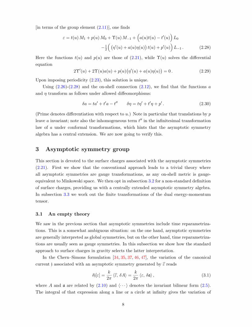
[in terms of the group element (2.11)], one finds
ε = t(u)M1 + p(u)M0 + Υ(u)M−1 +(a(u)t(u)− t′(u)
)L0
−12
( (η′(u) + a(u)η(u)
)t(u) + p′(u)
)L−1 . (2.28)
Here the functions t(u) and p(u) are those of (2.21), while Υ(u) solves the differential
equation
2Υ′(u) + 2Υ(u)a(u) + p(u)(η′(u) + a(u)η(u)
)= 0 . (2.29)
Upon imposing periodicity (2.23), this solution is unique.
Using (2.26)-(2.28) and the on-shell connection (2.12), we find that the functions a
and η transform as follows under allowed diffeomorphisms:
δa = ta′ + t′a− t′′ δη = tη′ + t′η + p′ . (2.30)
(Prime denotes differentiation with respect to u.) Note in particular that translations by p
leave a invariant; note also the inhomogeneous term t′′ in the infinitesimal transformation
law of a under conformal transformations, which hints that the asymptotic symmetry
algebra has a central extension. We are now going to verify this.
3 Asymptotic symmetry group
This section is devoted to the surface charges associated with the asymptotic symmetries
(2.21). First we show that the conventional approach leads to a trivial theory where
all asymptotic symmetries are gauge transformations, as any on-shell metric is gauge-
equivalent to Minkowski space. We then opt in subsection 3.2 for a non-standard definition
of surface charges, providing us with a centrally extended asymptotic symmetry algebra.
In subsection 3.3 we work out the finite transformations of the dual energy-momentum
tensor.
3.1 An empty theory
We saw in the previous section that asymptotic symmetries include time reparametriza-
tions. This is a somewhat ambiguous situation: on the one hand, asymptotic symmetries
are generally interpreted as global symmetries, but on the other hand, time reparametriza-
tions are usually seen as gauge symmetries. In this subsection we show how the standard
approach to surface charges in gravity selects the latter interpretation.
In the Chern–Simons formulation [34, 35, 37, 46, 47], the variation of the canonical
current j associated with an asymptotic symmetry generated by ε reads
δj[ε] =k
2π〈ε, δA〉 =
k
2π〈ε, δa〉 , (3.1)
where A and a are related by (2.10) and 〈· · · 〉 denotes the invariant bilinear form (2.5).
The integral of that expression along a line or a circle at infinity gives the variation of
8
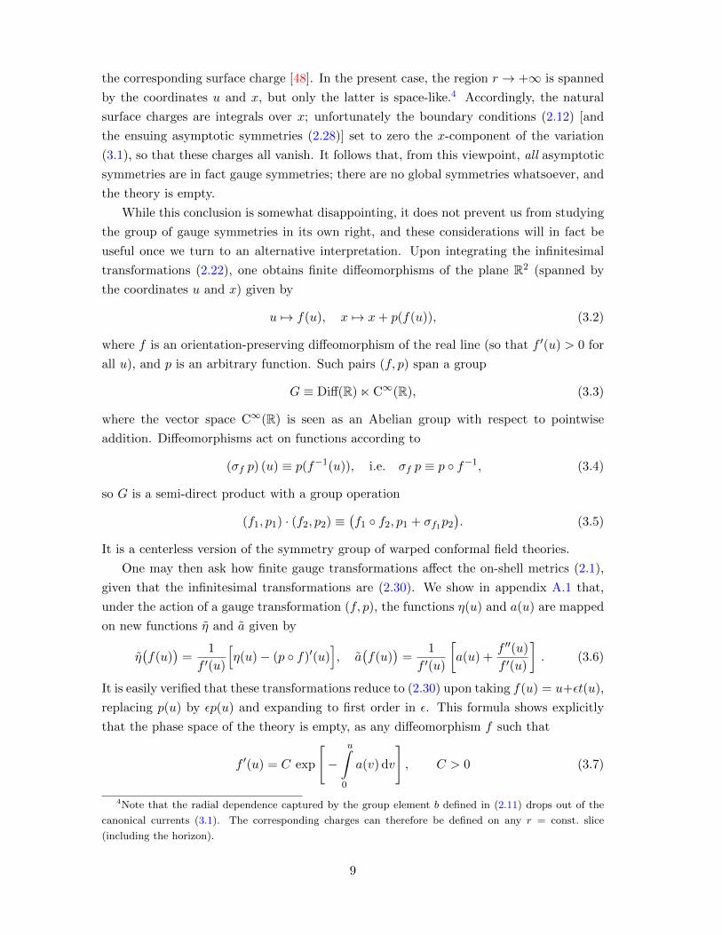
the corresponding surface charge [48]. In the present case, the region r → +∞ is spanned
by the coordinates u and x, but only the latter is space-like.4 Accordingly, the natural
surface charges are integrals over x; unfortunately the boundary conditions (2.12) [and
the ensuing asymptotic symmetries (2.28)] set to zero the x-component of the variation
(3.1), so that these charges all vanish. It follows that, from this viewpoint, all asymptotic
symmetries are in fact gauge symmetries; there are no global symmetries whatsoever, and
the theory is empty.
While this conclusion is somewhat disappointing, it does not prevent us from studying
the group of gauge symmetries in its own right, and these considerations will in fact be
useful once we turn to an alternative interpretation. Upon integrating the infinitesimal
transformations (2.22), one obtains finite diffeomorphisms of the plane R2 (spanned by
the coordinates u and x) given by
u 7→ f(u), x 7→ x+ p(f(u)), (3.2)
where f is an orientation-preserving diffeomorphism of the real line (so that f ′(u) > 0 for
all u), and p is an arbitrary function. Such pairs (f, p) span a group
G ≡ Diff(R) n C∞(R), (3.3)
where the vector space C∞(R) is seen as an Abelian group with respect to pointwise
addition. Diffeomorphisms act on functions according to
(σf p) (u) ≡ p(f−1(u)), i.e. σf p ≡ p ◦ f−1, (3.4)
so G is a semi-direct product with a group operation
(f1, p1) · (f2, p2) ≡(f1 ◦ f2, p1 + σf1p2
). (3.5)
It is a centerless version of the symmetry group of warped conformal field theories.
One may then ask how finite gauge transformations affect the on-shell metrics (2.1),
given that the infinitesimal transformations are (2.30). We show in appendix A.1 that,
under the action of a gauge transformation (f, p), the functions η(u) and a(u) are mapped
on new functions η and a given by
η(f(u)
)=
1
f ′(u)
[η(u)− (p ◦ f)′(u)
], a
(f(u)
)=
1
f ′(u)
[a(u) +
f ′′(u)
f ′(u)
]. (3.6)
It is easily verified that these transformations reduce to (2.30) upon taking f(u) = u+εt(u),
replacing p(u) by εp(u) and expanding to first order in ε. This formula shows explicitly
that the phase space of the theory is empty, as any diffeomorphism f such that
f ′(u) = C exp
[−
u∫0
a(v) dv
], C > 0 (3.7)
4Note that the radial dependence captured by the group element b defined in (2.11) drops out of the
canonical currents (3.1). The corresponding charges can therefore be defined on any r = const. slice
(including the horizon).
9
maps a(u) on a = 0. When combining this map with a suitable translation p(u), the whole
metric (2.1) is mapped on that of Minkoswki space, so that indeed any solution is pure
gauge. Note that the inhomogeneous term proportional to f ′′/f ′ in the transformation
law of a is crucial in order for the latter statement to be true.
In principle one can impose suitable fall-off conditions on the functions a(u) and η(u)
at future and past infinity, and study the subgroup of (3.3) that preserves these conditions.
For example, a(u) ∼ const.+O(1/|u|) would include Rindler spacetime, potentially leading
to interesting asymptotic symmetries at |u| → +∞. We will not follow this approach here;
instead, we will try to make the theory non-trivial by using an unconventional prescription
for the definition of surface charges.
3.2 Quasi-Rindler currents and charges
In the previous subsection we interpreted asymptotic symmetries as gauge symmetries,
in accordance with the fact that all surface charges written as integrals over a space-like
slice at infinity vanish. However, another interpretation is available: instead of integrating
(3.1) over x, we may decide to integrate it over retarded time u. Despite clashing with
the usual Hamiltonian formalism, this approach is indeed the most natural one suggested
by the u-dependent asymptotic Killing vector fields (2.21) and the solutions (2.1).
For convenience we will also assume that the coordinate u is periodic as in (2.23).
This condition introduces closed time-like curves and breaks Poincare symmetry (even
when a = 0 !); it sets off our departure from the world of Rindler to that of quasi-Rindler
holography. While it seems unnatural from a gravitational/spacetime perspective, this
choice is naturally suggested by our asymptotic symmetries and our phase space. In
the remainder of this paper we explore its consequences, assuming in particular that the
functions t(u), p(u), η(u) and a(u) are 2πL-periodic. This will in fact lead us to study
new aspects of warped conformal field theories, which we believe are interesting in their
own right.
In the quasi-Rindler case, the variation of the surface charge associated with the sym-
metry transformation (t, p), evaluated on the metric (a, η), reads
δQ(a,η)[t, p] =
2πL∫0
du δ ju . (3.8)
Using (3.1) and inserting expressions (2.12) and (2.28) yields
δQ(a,η)[t, p] =k
2π
2πL∫0
du(t(u) δT (u) + p(u) δP (u)
), (3.9)
where
T (u) = η′(u) + a(u)η(u), P (u) = a(u) , (3.10)
10
so that the charges are finite and integrable:
Q(a,η)[t, p] =k
2π
2πL∫0
du(t(u)T (u) + p(u)P (u)
). (3.11)
This expression shows in particular that the space of solutions (a, η) is dual to the asymp-
totic symmetry algebra5 [18, 49–51]. More precisely, the pair of functions (T (u), P (u))
transforms under the coadjoint representation of the asymptotic symmetry group, with
T (u) dual to time reparametrizations and P (u) dual to translations of x. This observation
will be crucial when determining the transformation law of T (u) and P (u) under finite
asymptotic symmetry transformations, which in turn will lead to a Cardy-like entropy
formula.
From the variations (2.30) of the functions (a, η), we deduce corresponding variations
of the functions T and P in (3.10):
δ(t,p)P = tP ′ + t′P − t′′, δ(t,p)T = tT ′ + 2t′T + p′P + p′′. (3.12)
This result contains all the information about the surface charge algebra, including its
central extensions. On account of 2πL-periodicity in the retarded time u, we can introduce
the Fourier-mode generators
Tn ≡kL
2π
2πL∫0
du einu/L T (u) Pn ≡k
2π
2πL∫0
du einu/L P (u) , (3.13)
whose Poisson brackets, defined by [Qξ, Qζ ] = −δξQζ , read
i[Tn, Tm] = (n−m)Tn+m , (3.14a)
i[Tn, Pm] = −mPn+m − iκ n2 δn+m,0 , (3.14b)
i[Pn, Pm] = 0 , (3.14c)
with κ = k. As it must be for a consistent theory, this algebra coincides with the Lie
bracket algebra (2.25) of allowed diffeomorphisms, up to central extensions. Note that
T0/L, being the charge that generates time translations u 7→ u + const, should be inter-
preted as the Hamiltonian, while P0 is the momentum operator (it generates translations
x 7→ x+ const). The only central extension in (3.14) is a twist term in the mixed commu-
tator; it is a non-trivial 2-cocycle [52]. In particular, it cannot be removed by redefinitions
of generators since the u(1) current algebra has a vanishing level.
5Note that the change of variables (3.10) is invertible for functions on the circle: given the functions a
and η, Eq. (3.10) specifies T and P uniquely; conversely, given some functions T and P , the functions a
and η ensuring that (3.10) holds are unique provided one imposes 2πL-periodicity of the coordinate u.
11
3.3 Warped Virasoro group and coadjoint representation
As a preliminary step towards the computation of quasi-Rindler entropy, we now work out
the finite transformation laws of the functions T and P . For the sake of generality, we will
display the result for arbitrary central extensions of the warped Virasoro group, including
a Virasoro central charge and a u(1) level. We will use a 2πL-periodic coordinate u, but
our end result (3.17)-(3.18) actually holds independently of that assumption.
Finite transformations of the stress tensor
The asymptotic symmetry group for quasi-Rindler holography is (3.3) with R replaced by
S1, and it consists of pairs (f, p), where p is an arbitrary function on the circle and f is a
diffeomorphism of the circle; in particular,
f(u+ 2πL) = f(u) + 2πL. (3.15)
(For instance, the diffeomorphisms defined by (3.7) are generally forbidden once that
condition is imposed.) However, in order to accommodate for inhomogeneous terms such
as those appearing in the infinitesimal transformations (2.30), we actually need to study
the central extension of this group. We will call this central extension the warped Virasoro
group, and we will denote it by G. Its Lie algebra reads
i[Tn, Tm] = (n−m)Tn+m +c
12n3 δn+m,0 (3.16a)
i[Tn, Pm] = −mPn+m − iκ n2 δn+m,0 (3.16b)
i[Pn, Pm] = K nδn+m,0 , (3.16c)
and is thus an extension of (3.14) with a Virasoro central charge c and a u(1) level K.
Note that, when K 6= 0, the central term in the mixed commutator [T, P ] can be removed
by defining Ln ≡ Tn + iκKnPn. In terms of generators Ln and Pn, the algebra takes the
form (3.16) without central term in the mixed bracket, and with a new Virasoro central
charge c′ = c− 12κ2/K. [We will see an illustration of this in eq. (5.11), in the context of
quasi-Rindler gravity in AdS3.] But when K = 0 as in (3.14), there is no such redefinition.
We relegate to appendix A.1 the exact definition of the warped Virasoro group G,
together with computations related to its adjoint and coadjoint representations. Here we
simply state the result that is important for us, namely the finite transformation law of the
stress tensor T and the u(1) current P . By construction, these transformations coincide
with the coadjoint representation of G, written in eqs. (A.21)-(A.22); thus, under a finite
transformation (3.2), the pair (T, P ) is mapped to a new pair (T , P ) with
T (f(u)) =1
(f ′(u))2
[T (u) +
c
12k{f ;u} − P (u)(p ◦ f)′(u)
−κk
(p ◦ f)′′(u) +K
2k((p ◦ f)′(u))2
](3.17)
P (f(u)) =1
f ′(u)
[P (u) +
κ
k
f ′′(u)
f ′(u)− K
k(p ◦ f)′(u)
], (3.18)
12
where {f ;u} is the Schwarzian derivative (A.10) of f . These transformations extend those
of a standard warped CFT [39], which are recovered for κ = 0. In the case of quasi-Rindler
spacetimes, we have c = K = 0 and κ is non-zero, leading to
T (f(u)) =1
(f ′(u))2
[T (u)− P (u)(p ◦ f)′(u)− κ
k(p ◦ f)′′(u)
](3.19)
P (f(u)) =1
f ′(u)
[P (u) +
κ
k
f ′′(u)
f ′(u)
](3.20)
which (for κ = k) actually follows from (3.6) and the definition (3.10). Note that these
formulas are valid regardless of whether u is periodic or not! In the latter case, f(u) is a
diffeomorphism of the real line.
Modified Sugawara construction
Before going further, we note the following: since P (u) is a Kac-Moody current, one
expects that a (possibly modified) Sugawara construction might convert some quadratic
combination of P ’s into a CFT stress tensor. This expectation is compatible with the
fact that P (u) du is a one-form, so that P (u) du⊗ P (u) du is a quadratic density. Let us
therefore define
M(u) ≡ k2
2κ(P (u))2 + k P ′(u) (3.21)
and ask how it transforms under the action of (f, p), given that the transformation law of
P (u) is (3.20). Writing this transformation as M 7−→ M, the result is
M(f(u)) =1
(f ′(u))2
[M(u) + κ {f ;u}
], (3.22)
which is the transformation law of a CFT stress tensor with central charge
cM ≡ 12κ = 12k =3
GN. (3.23)
Once more, this observation is independent of whether the coordinate u is periodic or not.
This construction is at the core of a simple relation between the quasi-Rindler sym-
metry algebra (3.14) and the BMS3 algebra. Indeed, by quadratically recombining the
generators Pn thanks to a twisted Sugawara construction
Mn =1
2κ
∑q∈Z
Pn−qPq − inPn , (3.24)
the brackets (3.14) reproduce the centrally extended BMS3 algebra [8]:
i[Tn, Tm] = (n−m)Tn+m (3.25a)
i[Tn, Mm] = (n−m)Mn+m +cM12
n3 δn+m, 0 (3.25b)
i[Mn, Mm] = 0. (3.25c)
13
This apparent coincidence implies that the representations of the warped Virasoro group
(with vanishing Kac-Moody level) are related to those of the BMS3 group, but one should
keep in mind that the similarity of group structures does not imply similarity of the physics
involved; in particular, the Hamiltonian operator in (3.25) is (proportional to) T0, while the
standard BMS3 Hamiltonian is M0. Nevertheless, unitary representations of the warped
Virasoro group with vanishing Kac-Moody level K can indeed be studied and classified
along the same lines as for BMS3 [18]. As we do not use these results in the present work
we relegate this discussion to appendix A.2.
4 Quasi-Rindler thermodynamics
In this section we study quasi-Rindler thermodynamics, both microscopically and macro-
scopically, assuming throughout that surface charges are defined as integrals over time
and that the coordinate u is 2πL-periodic. We start in subsection 4.1 with a microscopic,
Cardy-inspired derivation of the entropy of zero-mode solutions. Section 4.2 is devoted to
certain geometric aspects of boosted Rindler spacetimes, for instance their global Killing
vectors, which has consequences for our analytic continuation to Euclidean signature in
subsection 4.3. In subsection 4.4 we evaluate the on-shell action to determine the free
energy, from which we then derive other thermodynamic quantities of interest, such as
macroscopic quasi-Rindler entropy. In particular, we exhibit the matching between the
Cardy-based computation and the purely gravitational one.
4.1 Modular invariance and microscopic entropy
Here, following [39], we switch on chemical potentials (temperature and velocity) and
compute the partition function in the high-temperature limit, assuming the validity of a
suitable version of modular invariance. Because the u(1) level vanishes in the present case,
the modular transformations will not be anomalous, in contrast to standard behaviour in
warped CFT [39]. (This will no longer be true in AdS3 — see section 5.)
The grand canonical partition function of a theory at temperature 1/β and velocity η
is
Z(β, η) = Tr(e−β(H−ηP )
), (4.1)
where H and P are the Hamiltonian and momentum operators (respectively), and the
trace is taken over the Hilbert space of the system. In the present case, the Hamiltonian
is the (quantization of the) charge (3.11) associated with t(u) = 1 and p(u) = 0, i.e. the
zero-mode of T (u) up to normalization:
H =k
2π
2πL∫0
duT (u) . (4.2)
14
As for the momentum operator, it is the zero-mode of P (u) (again, up to normalization).
If we denote by I the Euclidean action of the system, the partition function (4.1) can
be computed as the integral of e−I+η∫dτP over paths in phase space that are periodic in
Euclidean time τ with period β. Equivalently, if we assume that the phase space contains
one Lagrange variable at each point of space (i.e. that we are dealing with a field theory),
the partition function may be seen as a path integral of e−I over fields φ that satisfy
φ(τ + β, x) = φ(τ, x + iβη) since P is the generator of translations along x. Note that
both approaches require the combination H − ηP to be bounded from below; in typical
cases (such as AdS, where P is really an angular momentum operator and η is an angular
velocity), this is a restriction on the allowed velocities of the system.
Now, our goal is to find an asymptotic expression for the partition function at high
temperature. To do this, we will devise a notion of modular invariance (actually only
S-invariance), recalling that the symmetries of our theory are transformations of (the
complexification of) S1×R of the form (3.2). Seeing the partition function (4.1) as a path
integral, the variables that are integrated out live on a plane R2 spanned by coordinates
u and x subject to the identifications
(u, x) ∼ (u+ iβ, x− iβη) ∼ (u+ 2πL, x) . (4.3)
The transformations
u =2πiL
βu x = x+ η u (4.4)
map these identifications on
(u, x) ∼ (u− 2πL, x) ∼(u+ i
(2πL)2
β, x+ 2πLη
). (4.5)
While the transformations (4.4) do not belong to the group of finite asymptotic symmetry
transformations (3.2), their analogues in the case of CFT’s, BMS3-invariant theories and
warped CFT’s [14, 39] apparently lead to the correct entropy formulas. We shall assume
that the same is true here, which implies that the partition function Z(β, η) satisfies a
property analogous to self-reciprocity,
Z(β, η) = Z
((2πL)2
β,iβη
2πL
). (4.6)
This, in turn, gives the asymptotic formula
Z(β, η)β→0+∼ exp
[−(2πL)2
β
(Hvac −
iβη
2πLPvac
)], (4.7)
where Hvac and Pvac are respectively the energy and momentum of the vacuum state.
These values can be obtained from the finite transformations (3.19) [with T = P = p = 0]
and (3.20) [with P = 0] by considering the map f(u) = Leinu/L with some integer n and
declaring that the vacuum value of the functions T (u) and P (u) is zero, exactly like for
15
the map between the plane and the cylinder in a CFT. Accordingly, the vacuum values of
these functions “on the cylinder”, say Tvac and Pvac, are
Tvac = 0 f ′(u)Pvac =in
L· κk, (4.8)
so that Hvac = 0. Choosing |n| 6= 1 introduces a conical excess (see subsection 4.3), or
equivalently gives a map u 7→ Leinu/L which is not injective, so the only possible choices
are n = ±1. Using Pvac = k2π
∫df Pvac(f(u)) = k
2π
∫ 2πL0 du f ′Pvac then establishes
Pvac = ±iκ for n = ±1 . (4.9)
The asymptotic expression (4.7) of the partition function thus becomes
Z(β, η)β→0+∼ e2πLκ|η| , (4.10)
where the sign of the dominant vacuum value in (4.9) is determined by the sign of η. (More
precisely, the vacuum ±iκ is selected when sign(η) = ∓1.) The free energy F ≡ −T logZ
is given by
F ≈ −2πκL |η|T (4.11)
at high temperature, and the corresponding entropy is
S = −∂F∂T
∣∣∣∣η
≈ 2πκL|η| = 2πkL|η| = 2πL|η|4GN
. (4.12)
In subsection 4.4 we will see that this result exactly matches that of a macroscopic
(i.e. purely gravitational) computation. Before doing so, we study Euclidean quasi-Rindler
spacetimes and elucidate the origin of the vacuum configuration (4.8).
4.2 Boosted Rindler spacetimes and their Killing vectors
Any solution of 3-dimensional Einstein gravity is locally flat and therefore locally has six
Killing vector fields. However, these vector fields may not exist globally. We now discuss
global properties of the Killing vectors of the geometry defined by the line-element (2.1)
with the identification (2.23). For simplicity, we present our results only for zero-mode
solutions, a, η = const.
The six local Killing vector fields are
ξ1 = ∂u ξ4 = eau(∂u − η∂x − (ar + 1
2 η2)∂r
)(4.13a)
ξ2 = ∂x ξ5 = a(ηu+ x)ξ3 − e−au∂x (4.13b)
ξ3 = e−au∂r ξ6 = a(ηu+ x)ξ4 + eau(ar + 1
2 η2)∂x . (4.13c)
Globally, due to our identification (2.23), only the Killing vectors ξ1 and ξ2 survive for
generic values of a. The only exception arises for specific imaginary values of Rindler
acceleration,
a =in
L0 6= n ∈ Z , (4.14)
16
in which case ξ3 and ξ4 are globally well-defined as well. If in addition η = 0, then all six
Killing vector fields can be defined globally. The non-vanishing Lie brackets between the
Killing vectors are
[ξ1, ξ3] = −[ξ2, ξ5] = −aξ3 [ξ1, ξ5] = aηξ3 − aξ5 (4.15a)
[ξ1, ξ4] = [ξ2, ξ6] = aξ4 [ξ1, ξ6] = aηξ4 + aξ6 (4.15b)
[ξ3, ξ6] = [ξ4, ξ5] = aξ2 [ξ5, ξ6] = aηξ2 − aξ1 . (4.15c)
This algebra is isomorphic to isl(2), as displayed in (2.4), with the identifications M0 = ξ2,
M+ = −2ξ4, M− = −ξ3, L0 = (−ξ1 + ηξ2)/a, L+ = 2(ξ6 + ηξ4)/a, L− = −(ξ5 + ηξ3)/a.
In terms of the generators tn, pn of the asymptotic Lie bracket algebra (2.25) we have
the identifications t0 ∼ ξ1, p0 ∼ ξ2, t1 ∼ ξ4 and p−1 ∼ ξ5; the vector field ξ3 generates
trivial symmetries, while the Killing vector ξ6 is not an asymptotic Killing vector, as it
is incompatible with the asymptotic behavior (2.21). This shows in particular that the
boundary conditions of quasi-Rindler gravity actually break Poincare symmetry even when
the coordinate u is not periodic. Interestingly, the four generators t0, t1, p−1, p0 obey the
harmonic oscillator algebra
i[α, α†] = z i[H, α] = −α i[H, α†] = α† (4.16)
where the Hamiltonian is formally given by t0 = H = α†α+const., the annihilation/creation
operators formally by t1 = α, p−1 = α† and p0 = z commutes with the other three gener-
ators. The algebra is written here in terms of Poisson brackets, but becomes the standard
harmonic oscillator algebra after quantization. Note, however, that t1 and p−1 are not
generally adjoint to each other.6 In the canonical realization (3.14) the first commutator
acquires an important contribution from the central extension
i[T1, P−1] = P0 − iκ . (4.17)
If we wish to identify the vacuum as the most symmetric solution then our vacuum
spacetime takes the form
ds2 = −2in r
Ldu2 − 2 dudr + dx2 (4.18)
with some non-zero integer n. We shall demonstrate in subsection 4.3 that |n| = 1 is the
only choice consistent with the u-periodicity (2.23). Thus, we have uncovered yet another
unusual feature of quasi-Rindler holography: the vacuum metric (4.18) with |n| = 1 is
complex. Our vacuum is neither flat spacetime (as one might have guessed naively) nor a
specific Rindler spacetime, but instead it is a Rindler-like spacetime with a specific imag-
inary Rindler “acceleration”, the value of which depends on the choice of the periodicity
6More precisely, they are certainly not each other’s adjoint in a unitary representation, although we
seem to be dealing with a non-unitary representation anyway (the vacuum value of P0 is imaginary).
17
L in (2.23). Another way to see that the solution a = η = 0 is not maximally symmetric
for finite L is to consider the six local Killing vectors ξ(0)i in the limit a, η → 0:
ξ(0)1 = ∂u ξ
(0)4 = u∂u − r∂r (4.19a)
ξ(0)2 = ∂x ξ
(0)5 = u∂x + x∂r (4.19b)
ξ(0)3 = ∂r ξ
(0)6 = x∂u + r∂x (4.19c)
Only four of them can be defined globally, because ξ(0)4 and ξ
(0)5 have a linear dependence
on u that is incompatible with finite 2πL-periodicity (2.23).
While the vacuum metric (4.18) (with n = 1) is preserved by all six Killing vectors
(4.13c), at most three of the associated generators of the asymptotic symmetry algebra
can annihilate the vacuum; since we expect from the discussion in subsection 4.1 that P0
is non-zero we pick the vacuum by demanding that T0, T1 and P−1 annihilate it. The
generator P0 then acquires a non-zero eigenvalue due to the central term in (4.17),
T0|0〉 = T1|0〉 = P−1|0〉 = [T1, P−1]|0〉 = 0 ⇒ P0|0〉 = iκ|0〉 =i
4GN|0〉 (4.20)
while the remaining two Killing vectors are excluded for reasons stated above (one acts
trivially, while the other violates the boundary conditions for asymptotic Killing vectors).
In fact, upon performing a shift P0 → P0 − iκ, the symmetry algebra (3.14) becomes
i[Tn, Tm] = (n−m)Tn+m , (4.21a)
i[Tn, Pm] = −mPn+m − iκ n(n− 1) δn+m,0 , (4.21b)
i[Pn, Pm] = 0 (4.21c)
so that the vacuum is now manifestly invariant under T0, T1, P0 and P−1.
These considerations reproduce the result (4.9) and thereby provide a consistency
check. The fact that the eigenvalue of P0 is imaginary indicates that the warped Virasoro
group is represented in a non-unitary way if the assumption of self-reciprocity (4.6) holds.
4.3 Euclidean boosted Rindler
In order to prepare the ground for thermodynamics, we now study the Euclidean version
of the metrics (2.1). We consider only zero-mode solutions for simplicity. Then, defining
new coordinates
τ = u+1
2aln(2ar + η2
)y = x− η
2aln(2ar + η2
)ρ = r +
η2
2a, (4.22)
the line-element (2.1) becomes
− 2aρ dτ2 +dρ2
2aρ+(
dy + η dτ)2. (4.23)
18
For non-zero Rindler acceleration, a 6= 0, there is a Killing horizon at ρh = 0, or equiva-
lently at
r = rh = −η2
2a. (4.24)
The patch ρ > 0 coincides with the usual Rindler patch for positive Rindler acceleration
a. For negative a the patches ρ > 0 and ρ < 0 switch their roles. We assume positive a in
this work so that τ is a timelike coordinate in the limit r →∞.
The Euclidean section of the metric (4.23) is obtained by defining
tE = −iτ (4.25)
which yields the line-element
ds2 = 2aρ dt2E +dρ2
2aρ+(
dy + iη dtE)2. (4.26)
Demanding the absence of a conical singularity at ρ = 0 and compatibility with (2.23)
leads to the periodicities
(tE, y) ∼ (tE + β, y − iβη) ∼ (tE − 2πiL, y) . (4.27)
which are the Euclidean version of the periodicities (4.3), with the inverse temperature
β = T−1 given by
T =a
2π. (4.28)
Given the periodicities (4.27), we can now ask which values of n in (4.14) give rise to
a regular spacetime with metric (4.18). Consider the Euclidean line-element (4.26) and
define another analytic continuation,
a =in
Lτ = itE ρ = −iρ sign(n) , (4.29)
which yields
ds2 =2|n|ρdτ2
L+Ldρ2
2|n|ρ+(
dy + η dτ)2. (4.30)
with the periodicities
(τ, y) ∼ (τ + iβ, y − iβη) ∼ (τ + 2πL, y) . (4.31)
The point now is that the Euclidean line-element (4.30) with the periodicities (4.31) has a
conical singularity at ρ = 0 unless |n| = 1. Thus, we conclude that the vacuum spacetime
(in the sense of being singularity-free and maximally symmetric) is given by (4.18) with
|n| = 1, confirming our discussion in sections 4.1 and 4.2.
19
4.4 Macroscopic free energy and entropy
The saddle point approximation of the Euclidean path integral leads to the Euclidean
partition function, which in turn yields the free energy. The latter is given by temperature
times the Euclidean action (2.20) evaluated on-shell:
F = −T 1
8πGN
−i2πL∫0
dtE
iβ|η|∫0
dy√γK∣∣ρ→∞ = −2πL|η|T
4GN, (4.32)
where we have inserted the periodicities from subsection 4.3 and used√γK = a+O(1/ρ).
The absolute value for η was introduced in order to ensure a positive volume form7 for
positive L and β.
From this result we extract the entropy
S = −∂F∂T
∣∣∣∣η
=2πL|η|4GN
, (4.33)
which coincides with the Cardy-based result (4.12). As a cross-check, we derive the same
expression in the Chern–Simons formulation by analogy to the flat space results [23]:
S =k
2π
−i2πL∫0
du
iβ|η|∫0
dx 〈AuAx〉 = k Lβ|η| 〈auax〉 = 2πk L|η| = 2πL|η|4GN
. (4.34)
We show in the next section that the same matching occurs in Rindler-AdS.
5 Boosted Rindler-AdS
In this section we generalize the discussion of the previous pages to the case of Rindler-
AdS spacetimes. In subsection 5.1 we establish quasi-Rindler-AdS boundary conditions
and show that the asymptotic symmetry algebra can be untwisted to yield a standard
warped CFT algebra, with a u(1) level that vanishes in the limit of infinite AdS radius.
Then, in subsection 5.2 we derive the entropy microscopically, and we show in subsection
5.3 that the same result can be obtained macroscopically.
5.1 Boundary conditions and symmetry algebra
We can deform the metric (2.1) to obtain a solution of Einstein’s equations Rµν− 12 gµνR =
gµν/`2 with a negative cosmological constant Λ = −1/`2,
ds2 = −2a(u)r du2 − 2 dudr + 2(η(u) + 2r/`) dudx+ dx2 . (5.1)
7 One pragmatic way to get the correct factors of i is to insert the Euclidean periodicities in the ranges
of the integrals and to demand again positive volume when integrating the function 1. In the flat space
calculation this implies integrating u from 0 to β, while here it implies integrating u from 0 to −i2πL.
20
Starting from this ansatz, we now adapt our earlier discussion to the case of a non-
vanishing cosmological constant. Since the computations are very similar to those of the
quasi-Rindler case, we will simply point out the changes that arise due to the finite AdS
radius. When we do not mention a result explicitly we imply that it is the same as for the
flat configuration; in particular we assume again 2πL-periodicity in u.
The Chern–Simons formulation is based on the deformation of the isl(2) algebra to
so(2, 2), where the translation generators no longer commute so that the last bracket in
(2.4) is replaced by
[Mn, Mm] =1
`2(n−m)Ln+m . (5.2)
The on-shell connection (2.10)-(2.12) and the asymptotic symmetry generators (2.27)-
(2.29) are modified as
a→ a + ∆a/` , ε→ ε+ ∆ε/` and b = exp[r2
(M−1 − 1
`L−1) ]
(5.3)
where
∆a = duL1 − dxL0 + 12η(u) dxL−1 (5.4a)
∆ε = t(u)L1 − p(u)L0 −Υ(u)L−1 . (5.4b)
The connection A changes correspondingly as compared to (2.13),
A→ A+ ∆A/` ∆A = ∆a− dr
2L−1 + r
(1` L−1 dx−M−1 dx− 1
2 a(u)L−1 du). (5.5)
Note in particular that all quadratic terms in r cancel due to the identity [L−1, [L−1, a]]−2`[L−1, [M−1, a]] + `2[M−1, [M−1, a]] = 0. Plugging the result (5.5) into the line-element
(2.6) yields
ds2 → ds2 + ∆ ds2/` ∆ ds2 = 4r dudx (5.6)
thus reproducing the solution (5.1).
Consequently, the variations of the functions a(u) and η(u) in (2.30) are also modified,
δa(u)→ δa(u)− 2p′(u)/` , (5.7)
δη(u)→ δη(u) + 2p(u)η(u)/`+ 4Υ(u)/` . (5.8)
Using (2.29), one can show that the presence of the last term in the second line does not
affect the transformation of the function T (u) defined in (3.10). Moreover, the charges
(3.11) remain unchanged. In fact, in the Rindler-AdS case only the transformation of the
current P is deformed as
δpP = −2p′/` , (5.9)
which leads to the following Poisson brackets of the charges Pn defined in (3.13):
i[Pn, Pm] = −2k
`n δn+m,0 . (5.10)
21
In particular, the limit `→∞ reproduces the algebra (3.14).
At finite ` the presence of the non-vanishing level in (5.10) enables us to remove the
central extension of the mixed bracket of (3.14b) thanks to a twist
Ln = Tn −i`κ
2knPn (5.11)
in terms of which the asymptotic symmetry algebra reads
i[Ln, Lm] = (n−m)Ln+m +c
12n3 δn+m,0 (5.12a)
i[Ln, Pm] = −mPn+m (5.12b)
i[Pn, Pm] = −2k
`n δn+m,0 (5.12c)
with the expected Brown–Henneaux central charge8 [4]
c = 6κ2
k` = 6k` =
3`
2GN. (5.13)
5.2 Microscopic quasi-Rindler-AdS entropy
As in the case of a vanishing cosmological constant, it is possible to derive a Cardy-
like entropy formula that can be applied to zero-mode solutions. The only difference with
respect to subsection 4.1 is the non-vanishing u(1) level K = −2k/` that leads to a slightly
different form of modular invariance. Namely, according to [39], the self-reciprocity of the
partition function, eq. (4.6), now becomes
Z(β, η) = eβKLη2/2Z
((2πL)2
β,iβη
2πL
)(5.14)
leading to the high-temperature free energy
F ≈ (2πL)2
β2
(Hvac −
iβη
2πLPvac
)−KLη2/2 . (5.15)
(We have renamed the chemical potential conjugate to P0 as η for reasons that will become
clear in subsection 5.3.) This is the same as in (4.7), up to a temperature-independent
constant proportional to the u(1) level. The vacuum values of the Hamiltonian and the
momentum operator are once more given by the arguments above (4.8); in particular, the
u(1) level plays no role for these values. Accordingly, the free energy at high temperature
T = β−1 � 1 boils down to
F ≈ −2πLk|η|T + kLη2/` (5.16)
and the corresponding entropy is again given by (4.12):
S =2πL|η|4GN
(5.17)
8This central charge is expected to be shifted quantum mechanically at finite k` [43]. Since we are
interested in the semi-classical limit here, we shall not take such a shift into account.
22
Notably, this is independent of the AdS radius. The same result can be obtained by
absorbing the twist central charge through the redefinition (5.11) and then using the
Cardy-like entropy formula derived in [39]. In the next subsection we show that this
result coincides with the gravitational entropy, as in the flat quasi-Rindler case discussed
previously.
5.3 Macroscopic quasi-Rindler-AdS entropy
Generalizing the macroscopic calculations from section 4 for zero-mode solutions (5.3)
with constant a and η we find that the outermost Killing horizon is located at
rh =`
4
(√a2`2 + 4a`η − a`− 2η
)= −η
2
2a+O(1/`) (5.18)
and has a smooth limit to the quasi-Rindler result (4.24) for infinite AdS radius ` → ∞.
We assume η > −a`/4 so that rh is real and surface-gravity is non-zero.
The vacuum spacetime reads
ds2 = −2ir du2
L− 2 du dr +
4r
`dudx+ dx2 (5.19)
where again we defined “vacuum” as the unique spacetime compatible with our boundary
conditions, regularity and maximal symmetry.
Making a similar analytic continuation as in subsection 4.3 we obtain the line-element
ds2 = K(r) dt2E +dr2
K(r)+(
dy + i(2r/`+ η) dtE)2
(5.20)
with the Killing norm
K(r) =4r2
`2+
4ηr
`+ 2ar + η2 (5.21)
and the periodic identifications
(tE, y) ∼ (tE − 2πiL, y) ∼ (tE + β, y − iβη) (5.22)
where inverse temperature β = T−1 and boost parameter η are given by
T =
√a2 + 4aη/`
2πη =
√a2`2/4 + aη`− a`/2 . (5.23)
In particular, the chemical potential η no longer coincides with the parameter η appearing
in the metric. Note that the limit of infinite AdS radius is smooth and leads to the expres-
sions in subsection 4.3 for line-element, periodicities, temperature and boost parameter.
Converting the zero-mode solution (5.20)-(5.23) into the Chern-Simons formulation
and using formula (4.34) then yields the entropy
S =2πL|η|4GN
. (5.24)
23
where independence of the AdS radius follows from the fact that the connection given by
(5.4a) has no non-zero component along any of the Mn’s. This agrees with the microscopic
result (5.17).
The macroscopic free energy compatible with the first law dF = −S dT − P0 dη is
given by
F (T, η) = H(S, P0)− TS − P0η = −2πLk|η|T + kLη2/` (5.25)
where H is given by the zero mode charge T = aη through (4.2), H = kLaη = −F , and
P0 is given by the zero mode charge P = a through the right eq. (3.13), P0 = kLa. The
result (5.25) also coincides with the microscopic one (5.16).
6 Rindlerwahnsinn?
In this final section9 we highlight some of the unusual features that we unraveled in our
quest for near horizon holography. We add some comments, explanations and possible
resolutions of the open issues.
6.1 Retarded choices?
Let us summarize and discuss aspects of the dependence of Rindler acceleration on retarded
time. (Note that our whole paper can easily be sign-flipped to advanced time v, which
may be useful in some applications.)
Rindler acceleration depends on retarded time. We started with the ansatz (1.2)
since we wanted a state-dependent Rindler acceleration to accommodate a state-dependent
temperature. We left it open whether Rindler acceleration a was a function of retarded
time u, spatial coordinate x or both. The Einstein equations forced us to conclude that
Rindler acceleration can depend on retarded time only. We give now a physical reason
why this should be expected. Namely, if the zeroth law of black hole mechanics holds then
surface gravity (and thus Rindler acceleration) must be constant along the horizon. In
particular, it cannot depend on x. If the horizon changes, e.g. due to emission of Hawking
quanta or absorption of matter, then Rindler acceleration can change, which makes the
dependence on u natural, much like the corresponding dependence of Bondi mass on the
lightlike time.
Retarded time is periodic. While many of our results are actually independent of the
choice (2.23), it was still a useful assumption for several purposes, e.g. the introduction of
Fourier modes. For some physical observables it is possible to remove this assumption by
taking the limit L→∞. We shall provide an important example in section 6.2 below.
9 The play on words in this section title is evident for German speaking physicists; for the remaining
ones we point out that “Rinderwahnsinn” means “mad cow disease” and “Wahnsinn” means “madness”.
24
Boundary currents are integrated over retarded time. If we wanted our theory to
be non-empty we could not use the standard definition of canonical charges integrated over
space, but instead had to consider boundary currents integrated over retarded time. We
have no further comments on this issue, except for pointing out that in four dimensions,
a bilinear in the Bondi news is integrated over retarded time in order to yield the ADM
mass. Thus, despite of the clash with the usual Hamilton formulation we believe that we
have made here the most natural choice, given our starting point.
6.2 Rindler entropy?
Let us finally take a step back and try to connect with our original aim of setting up Rindler
holography and microscopically calculating the Rindler entropy [28]. We summarize in
appendix B results for Rindler thermodynamics and Rindler entropy, which match the
near horizon results of BTZ black holes and flat space cosmologies.
We consider a limiting procedure starting with our result for entropy (4.33). We are
interested in a limit where simultaneously the compactification length L in (2.23) tends
to infinity, the boost parameter η tends to zero, the length of the spatial cycle x appears
in the entropy and all unusual factors of i are multiplied by something infinitesimal. In
other words, we try to construct a limit towards Rindler entropy (B.12).
Consider the identifications (4.3) with a complexified β → β0 + 2πiL and split them
into real and imaginary parts:
Re : (u, x) ∼ (u, x+ 2πLη) ∼ (u+ 2πL, x) Im : (u, x) ∼ (u+ iβ0, x− iβ0η) (6.1)
The rationale behind this shift is that the real part of the periodicities untwists. As in
appendix B we call the (real) length of the x-cycle L and thus have the relation
L = 2πLη . (6.2)
Therefore, taking the decompactification limit for retarded time, L → ∞, while keeping
fixed L simultaneously achieves the desired η → 0, so that the periodicities (6.1) in this
limit simplify to
Re : (u, x) ∼ (u, x+ L) Im : (u, x) ∼ (u+ iβ0, x) (6.3)
which, if interpreted as independent periodicities, are standard relations for non-rotating
horizons at inverse temperature β0 and with a length of the spatial cycle given by L. Apart
from taking limits our only manipulation was to shift the inverse temperature β in the
complex plane. Thus, any observable that is independent from temperature should remain
unaffected by such a shift; moreover, the “compactification” of β along the imaginary axis
is then undone by taking the decompactification limit L → ∞. We conclude from this
that entropy S from (4.33) should have a smooth limit under all the manipulations above
and hopefully yield the Rindler result (B.12). This is indeed the case:
limL→∞,η→L/(2πL)(
limβ→β0+2πiL S)
=L
4GN. (6.4)
25
Thus, we recover the usual Bekenstein–Hawking entropy law as expected from Rindler
holography. In this work we have also provided a microscopic, Cardy-like derivation of
this result. A different singular limit was considered in [53], where the Rindler entropy
(6.4) was derived from a Cardy formula for holographic hyperscaling theories.
6.3 Other approaches
Relation to BMS/ultrarelativistic CFT. Using our quadratic map (3.24) of warped
CFT generators to BMS3 generators together with the result (3.23) for the central charge,
we now check what microstate counting would be given by an ultrarelativistic CFT (or
equivalently a Galilean CFT) [14]. Using the “angular momentum” hL = aη, the “mass”
hM = a2/(2k), the central charge cM = 12k with k = 1/(4GN ), and introducing an extra
factor of L to accommodate our periodicity (2.23), the ultrarelativistic Cardy formula
gives
SUCFT = 2πL |hL|√
cM24hM
= 2πL |aη|√k2
a2=
2πL|η|4GN
. (6.5)
This entropy thus coincides with the warped CFT entropy (4.12), and matches the gravity
result (4.33).
Other Rindler-type boundary conditions. While finishing this work the paper [54]
appeared which proposes alternative Rindler boundary conditions, motivated partly by
Hawking’s claim that the information loss paradox can be resolved by considering the
supertranslation of the horizon caused by ingoing particles [55].10 (See also [57,58].) In [54]
the state-dependent functions depend on the spatial coordinate and thus allow for standard
canonical charges. The corresponding Rindler acceleration (and thus temperature) is
state-independent and the asymptotic symmetry algebra has no central extension. We
checked that the Rindler acceleration of that paper can be made state-dependent, but in
accordance with our discussion in section 6.1 it cannot depend on the spatial coordinate;
only dependence on retarded/advanced time is possible. Thus, we believe that if one wants
to allow for a state-dependent temperature in Rindler holography the path described in
the present work is unavoidable.
Generalizations. We finish by mentioning a couple of interesting generalizations that
should allow in several cases straightforward applications of our results, like generaliza-
tions to higher derivative theories of (massive or partially massless) gravity, theories that
include matter and theories in higher dimensions. In particular, it would be interesting
to generalize our discussion to topologically massive gravity [59] in order to see how the
entropy computation would be affected.
10After posting this paper, a more detailed account of the relationship between near horizon proper-
ties and supertranslations was posted by Hawking, Perry and Strominger [56], where they argue that
supertranslations generate “soft hair” on black holes, where “soft” means “zero energy”.
26
Acknowledgments
We are grateful to Gaston Giribet for collaboration and for sharing his insights on Rindler
holography during the first two years of this project (August 2013 — June 2015). In
addition, we thank Glenn Barnich, Diego Hofman and Friedrich Scholler for discussions.
HA was supported in part by the Dutch stichting voor Fundamenteel Onderzoek der
Materie (FOM) and in part by the Iranian National Science Foundation (INSF). SD is a
Research Associate of the Fonds de la Recherche Scientifique F.R.S.-FNRS (Belgium). He
is supported in part by the ARC grant “Holography, Gauge Theories and Quantum Gravity
Building models of quantum black holes”, by IISN - Belgium (convention 4.4504.15) and
benefited from the support of the Solvay Family. He thanks Gaston Giribet and Buenos
Aires University for hosting him while this work was in progress. DG was supported by the
Austrian Science Fund (FWF), projects Y 435-N16, I 952-N16, I 1030-N27 and P 27182-
N27, and by the program Science without Borders, project CNPq-401180/2014-0. DG also
thanks Buenos Aires University for hosting a research visit, supported by OeAD project
AR 09/2013 and CONICET, where this work was commenced. BO was supported by the
Fund for Scientific Research-FNRS Belgium (under grant number FC-95570) and by a
research fellowship of the Wiener-Anspach Foundation.
A On representations of the warped Virasoro group
This appendix is devoted to certain mathematical considerations regarding the warped
Virasoro group. They are motivated by the questions encountered in section 3 of this
paper, although they are also interesting in their own right. First, in subsection A.1
we study the coadjoint representation of the warped Virasoro group, which is needed
to derive formulas (3.17)-(3.18) for the transformation law of the stress tensor. Then,
in subsection A.2 we classify all irreducible, unitary representations of this group with
vanishing u(1) level using the method of induced representations. We assume throughout
that the coordinate u is 2πL-periodic.
A.1 Coadjoint representation
We call warped Virasoro group, denoted G, the general central extension of the group
G = Diff+(S1) n C∞(S1), (A.1)
where the notation is the same as in (3.3) up to the replacement of R by S1 [so that in
particular f satisfies property (3.15)]. In this subsection we display an explicit definition of
G and work out its adjoint and coadjoint representations, using a 2πL-periodic coordinate
u to parametrize the circle. We refer to [52,60] for more details on the Virasoro group and
its cohomology.
27
Since the differentiable, real-valued second cohomology space of G is three-dimensional
[52,61], there are exactly three central extensions to be taken into account when defining
G; in other words, G ∼= G × R3 as manifolds. Accordingly, elements of G are pairs (f, p)
belonging to G, supplemented by triples of real numbers (λ, µ, ν). The group operation in
G is
(f1, p1;λ1, µ1, ν1) · (f2, p2;λ2, µ2, ν2) = (A.2)
=(f1 ◦ f2, p1 + σf1p2;λ1 + λ2 +B(f1, f2), µ1 + µ2 + C(f1, p2), ν1 + ν2 +D(f1, p1, p2)
),
where σ is the action (3.4) while B, C and D are non-trivial 2-cocycles on G given explicitly
by
B(f1, f2) = − 1
48π
∫S1
ln(f ′1 ◦ f2) d ln(f ′2) , (A.3)
C(f1, p2) = − 1
2π
∫S1
p2 · d ln(f ′1) , (A.4)
D(f1, p1, p2) = − 1
4π
∫S1
p1 · d(σf1p2) . (A.5)
In particular, B is the standard Bott–Thurston cocycle [60] defining the Virasoro group.
Adjoint representation and Lie brackets
To write down an explicit formula for the coadjoint representation of the warped Virasoro
group, we first need to work out the adjoint representation, which acts on the Lie algebra
g of G. As follows from the definition of G, that algebra consists of 5-tuples (t, p;λ, µ, ν)
where t = t(u) ∂∂u is a vector field on the circle, p = p(u) is a function on the circle, and
λ, µ, ν are real numbers. The adjoint representation of G, which we will denote as Ad, is
then defined as
Ad(f,p1;λ1,µ1,ν1)(t, p2;λ2, µ2, ν2) =
=d
dε
[(f, p1;λ1, µ1, ν1) ·
(eεt, εp2; ελ2, εµ2, εν2
)· (f, p1;λ1, µ1, ν1)−1
]∣∣ε=0
(A.6)
where eεt is to be understood as an infinitesimal diffeomorphism eεt(u) = u+εt(u)+O(ε2).
Given the group operation (A.2), it is easy to verify that the central terms λ1, µ1 and ν1
play a passive role, so we may simply set them to zero and write Ad(f,p;λ,µ,ν) ≡ Ad(f,p).
Using multiple Taylor expansions and integrations by parts, the right-hand side of (A.6)
28
yields
Ad(f,p1)(t, p2;λ, µ, ν) =
(Adf t, σfp2 + ΣAdf t p1; λ−
1
24π
2πL∫0
du t(u){f ;u},
µ− 1
2π
∫p2 · d ln(f ′) +
1
2π
2πL∫0
du t(u)
[(p1 ◦ f)′′ − (p1 ◦ f)′
f ′′
f ′
]∣∣∣∣u
,
ν − 1
2π
∫p1 · d(σfp2) +
1
4π
2πL∫0
du t(u)[(p1 ◦ f)′(u)
]2), (A.7)
where prime denotes differentiation with respect to u. Let us explain the meaning of the
symbols appearing here:
• The symbol Ad on the right-hand side denotes the adjoint representation of the
group Diff+(S1):
(Adf t) (u) ≡ d
dε
[f ◦ eεt ◦ f−1(u)
]∣∣ε=0
= f ′(f−1(u)) · t(f−1(u)) . (A.8)
The far right-hand side of this equation should be seen as the component of a vector
field (Adf t)(u) ddu . Equivalently,
(Adf t) (f(u)) = f ′(u) · t(u) , (A.9)
which is the usual transformation law of vector fields on the circle under diffeomor-
phisms.
• The quantity {f ;u} is the Schwarzian derivative of the diffeomorphism f evaluated
at u:
{f ;u} ≡
[f ′′′
f ′− 3
2
(f ′′
f ′
)2]∣∣∣∣∣u
. (A.10)
• The symbol Σ denotes the differential of the action σ of Diff+(S1) on C∞(S1).
Explicitly, if t is a vector field on the circle and if p ∈ C∞(S1),
(Σt p)(u) ≡ − d
dε[(σeεtp) (u)]|ε=0 = t(u) · p′(u) . (A.11)
It is easily verified, upon considering an infinitesimal diffeomorphism f and an infinites-
imal function p1, that the Lie brackets defined by this adjoint representation coincide with
the standard brackets of a centrally extended warped Virasoro algebra. More precisely,
upon defining the generators
Tn ≡(Leinu/L
∂
∂u, 0; 0, 0, 0
)Pn ≡
(0, einu/L; 0, 0, 0
)(A.12)
29
and the central charges
Z1 ≡ (0, 0; 1, 0, 0) Z2 ≡ (0, 0; 0, 1, 0) Z3 ≡ (0, 0; 0, 0, 1) (A.13)
the Lie brackets defined by
[(t1, p1;λ1, µ1, ν1), (t2, p2;λ2, µ2, ν2)] ≡ −d
dε
[Ad(eεt1 ,εp1;ελ1,εµ1,εν1)(t2, p2;λ2, µ2, ν2)
]∣∣∣ε=0
(A.14)
turn out to read
i[Tn, Tm] = (n−m)Tn+m +Z1
12n3δn+m,0 (A.15)
i[Tn, Pm] = −mPn+m − iZ2n2δn+m,0 (A.16)
i[Pn, Pm] = Z3nδn+m,0 . (A.17)
Here we recognize the centrally extended algebra (3.16), up to the fact that the central
charges Zi are written as operators; eventually they will be multiples of the identity, with
coefficients c, κ and K corresponding to Z1, Z2 and Z3 respectively.
Coadjoint representation
The coadjoint representation of G is the dual of the adjoint representation, and coincides
with the finite transformation laws of the functions T and P introduced in (3.10) [i.e. the
stress tensor and the u(1) current]. Explicitly, the dual g∗ of the Lie algebra g consists of
5-tuples
(T, P ; c, κ,K) (A.18)
where T = T (u) du ⊗ du is a quadratic density on the circle, P = P (u) du is a one-form
on the circle, and c, κ, K are real numbers — those are the values of the various central
charges. We define the pairing of g∗ with g by11
〈(T, P ; c, κ,K), (t, p;λ, µ, ν)〉 ≡ k
2π
2πL∫0
du(T (u)t(u)+P (u)p(u)
)+cλ+κµ+Kν , (A.19)
so that it coincides, up to central terms, with the definition of surface charges (3.11).
Note that here c is the usual Virasoro central charge, K is the u(1) level and κ is the twist
central charge appearing in (3.16). The coadjoint representation Ad∗ of G is defined by
Ad∗(f,p)(T, P ; c, κ,K) ≡ (T, P ; c, κ,K) ◦Ad(f,p)−1 .
Using the explicit form (A.7) of the adjoint representation, one can read off the transfor-
mation law of each component in (A.18). The result is
Ad∗(f,p)(T, P ; c, κ,K) =(
Ad∗(f,p)T,Ad∗(f,p)P ; c, κ,K)
(A.20)
11As usual [60, 62], what we call the “dual space” here is really the smooth dual space, i.e. the space of
regular distributions on the space of functions or vector fields on the circle.
30
(i.e. the central charges are left invariant by the action of G), where Ad∗(f,p)T and Ad∗(f,p)P
are a quadratic density and a one-form on the circle (respectively) whose components,
evaluated at f(u), are(Ad∗(f,p)T
)(f(u)) =
1
(f ′(u))2×
×[T (u) +
c
12k{f ;u} − P (u)(p ◦ f)′(u)− κ
k(p ◦ f)′′(u) +
K
2k((p ◦ f)′(u))2
](A.21)
and (Ad∗(f,p)P
)(f(u)) =
1
f ′(u)
[P (u) +
κ
k
f ′′(u)
f ′(u)− K
k(p ◦ f)′(u)
]. (A.22)
These are the transformation laws displayed in (3.17)-(3.18), with Ad∗(f,p)T ≡ T and
Ad∗(f,p)P ≡ P . They reduce to the transformations of a standard warped CFT [39] for
κ = 0. In the Rindler case, however, c = K = 0 and κ = k is non-zero.
The transformation law of the function η(u) in (3.6) under finite asymptotic symmetry
transformations can be worked out in a much simpler way. Indeed, it is easily verifed
that the left formula in (3.6) reproduces (2.30) for infinitesimal transformations, and is
compatible with the group operation (3.5) of the warped Virasoro group. One can also
check that the transformation laws (3.19) follow from (3.6) and the definition (3.10).
A.2 Induced representations
As indicated by the imaginary vacuum values (4.9) (which are actually fairly common in
the world of warped CFT’s [39]), the asymptotic symmetry group is not represented in a
unitary way in quasi-Rindler holography. Nevertheless, since the standard interpretation
of symmetries in quantum mechanics requires unitarity [63], it is illuminating to study
unitary representations of the warped Virasoro group. Here we classify such representa-
tions for the case of vanishing Kac-Moody level K, but non-vanishing twist κ. As in the
case of the Euclidean, Poincare or BMS groups, the semi-direct product structure (A.1) [or
similarly (3.9)] is crucial; indeed, all irreducible unitary representations of such a group are
induced a la Wigner [64, 65]. We refer to [66] for more details on induced representations
and we mostly use the notations of [18,19].
A lightning review of induced representations
The construction of induced representations of the warped Virasoro group G with vanishing
u(1) level follows the same steps as for the Poincare group [65,67] or the BMS3 group [18].
One begins by identifying the dual space of the Abelian group C∞(S1), which in the
present case consists of currents P (u) du. [The elements of this dual space are typically
called “momenta”, and our notation P (u) is consistent with that terminology.] One then
defines the orbit OP and the little group GP of P = P (u) du as
OP ≡{f · P | f ∈ Diff+(S1)
}and GP ≡
{f ∈ Diff+(S1) | f · P = P
}, (A.23)
31
where the action of f on P is given by (3.20). Then, given an orbit OP and an irreducible,
unitary representation R of its little group GP in some Hilbert space E , the corresponding
induced representation T acts on square-integrable wave functions Ψ : OP → E : q 7→ Ψ(q)
according to [66]
(T [(f, p)] Ψ) (q) ≡[ρf−1(q)
]1/2ei〈q,p〉R
[g−1q fgf−1·q
]Ψ(f−1 · q
), (A.24)
where (f, p) belongs to Diff+(S1) n C∞(S1). Let us briefly explain the terms of this
equation:
• The real, positive function ρf on OP denotes the Radon-Nikodym derivative of the
measure used to define the scalar product of wavefunctions. It is an “anomaly” that
takes the value ρf = 1 for all f when the measure is invariant, but otherwise depends
on f and on the point q at which it is evaluated. In simple cases (e.g. the Poincare
group), the measure is invariant and ρf (q) = 1 for all f and all q ∈ OP .
• The operator R[g−1q fgf−1·q
]is a “Wigner rotation”: it is the transformation corre-
sponding to f in the space of spin degrees of freedom of the representation T . We
denote by gq the “standard boost” associated with q, that is, a group element such
that gq · P = q. For scalar representations, R is trivial and one may simply forget
about the Wigner rotation.
The classification of irreducible, unitary representations of the central extension of Diff+(S1)nC∞(S1) with vanishing Kac-Moody level then amounts to the classification of all possible
orbits (A.23) and of all unitary representations of the corresponding little groups.
Induced representations of G
Our goal now is to classify all irreducible, unitary representations of the warped Vira-
soro group with vanishing Kac-Moody level, under the assumption that there exists a
quasi-invariant measure on all the orbits (see [68] for the construction of such measures).
According to the lightning review just displayed, this amounts to the classification of
orbits, as defined in (A.23). We start with two preliminary observations:
1. For any constant current P (u) = P0 = const, the little group GP consists of rigid
time translations f(u) = u+ u0.
2. The charge Q[P ] defined as
Q[P ] ≡ k
2π
2πL∫0
duP (u) (A.25)
is constant along any coadjoint orbit of the warped Virasoro group, regardless of
the values of the central charges c, κ and K. In other words, for any current P ,
32
any (orientation-preserving) diffeomorphism f of the circle and any function p, the
zero-mode of P is left invariant by the coadjoint action:
Q[Ad∗(f,p)P
]= Q[P ], (A.26)
where Ad∗(f,p)P is given by (3.18). This result holds, in particular, in the case
c = K = 0 that we wish to study, and corresponds physically to the fact that the
average value of acceleration is invariant under asymptotic symmetries.
The proof of both results is straightforward, as they can be verified by brute force. In fact,
they follow from a stronger statement: it turns out that the orbits OP foliate the space
of currents into hyperplanes of constant Q[P ], so that any current P (u) can be brought
to a constant by acting with a diffeomorphism. To prove this, note that constancy of
Q[P ] implies that that constant, if it exists, coincides with the zero-mode P0 of P (u).
The question thus boils down to whether or not there exists an orientation-preserving
diffeomorphism f such that
(f · P )|f(u)(3.6)=
1
f ′(u)
[P (u) +
κ
k
f ′′(u)
f ′(u)
]!
= P0 . (A.27)
This condition is equivalent to an inhomogeneous first-order differential equation for 1/f ′,
whose solution is
1
f ′(u)= A exp
kκ
u∫0
dv P (v)
− k
κP0
u∫0
dt exp
kκ
u∫t
dv P (v)
(A.28)
where A is a real parameter. Since u is assumed to be 2πL-periodic, this function must
be 2πL-periodic as well. This selects a unique solution (and such a solution exists for
any value of P0), meaning that, for any P (u), there always exists a diffeomorphism f of
the circle such that f · P be a constant12; furthermore, that diffeomorphism is uniquely
specified by P (u) up to a rigid time translation.
This proves that all orbits OP are hyperplanes specified by the value of the charge
(A.25), in accordance with the fact that P0 is a Casimir operator in (3.16). One can
then apply the usual machinery of induced representations to the warped Virasoro group,
and compute, for instance, the associated characters along the lines of [19]; however, as
the interpretation of these characters in the present context is unclear, we refrain from
displaying them.
12An alternative way to prove the same result is to recall the modified Sugawara construction (3.21), by
which a coadjoint orbit of the Virasoro group with non-negative energy is associated with each orbit OP .
Since the only Virasoro orbits with non-negative energy are orbits of constants, we know that there always
exists a diffeomorphism f that brings a given Sugawara stress tensor (3.21) into a constant, which in turn
brings the corresponding current P to a constant.
33
Physical properties of unitary representations
We have just seen that unitary representations of the warped Virasoro group [with vanish-
ing u(1) level] can be classified according to the possible values of the Casimir operator P0
in (3.16). Accordingly, the orbits (A.23) are affine hyperplanes with constant zero-modes
embedded in the space of currents P (u). In particular, each orbit contains exactly one
constant representative. The physical meaning of this statement is that any (generally
time-dependent) acceleration a(u) can be brought to a constant, a0, by using a suitable
reparametrization of time that preserves 2πL-periodicity. Furthermore, a0 coincides with
the Fourier zero-mode of a(u). Note that, with the requirement of 2πL-periodicity, it is no
longer true that any time-dependent acceleration a(u) can be mapped on a = 0 because
the diffeomorphisms defined by (3.7) generally do not preserve that requirement.
Having classified the orbits, we know, in principle, the irreducible unitary represen-
tations of the warped Virasoro group at vanishing Kac-Moody level. In three spacetime
dimensions, these representations describe the Hilbert space of metric fluctuations around
the background specified by the orbit OP and the representation R [18, 20, 49, 69], as fol-
lows from the fact that the phase space coincides with the coadjoint representation of the
asymptotic symmetry group. For instance, an induced representation of G specified by an
orbit OP and the trivial representation of the little group gives the Hilbert space of metric
fluctuations around the background
ds2 = −2P (u) r du2 − 2 du dr + dx2. (A.29)
Here u is still understood as a 2πL-periodic coordinate; in particular, the solution at a = 0
is not Minkowski spacetime because of that identification.
Note that, in any unitary representation of the type just described, the eigenvalues of
the Hamiltonian T0 are unbounded from below (and from above). There is thus a trade-off
between unitarity and boundedness of energy: if we insist that the representation be uni-
tary, then it is a (direct integral of) induced representation(s), and energy is unbounded
both from below and from above; conversely, if we insist that energy be bounded from
below, then the asymptotic symmetry group cannot act unitarily on the Hilbert space
of the putative dual theory. This property has actually been observed in representations
of the Galilean Conformal Algebra in two dimensions, gca2, and its higher-spin exten-
sions [17, 70]. Indeed, when T0 is interpreted as the Hamiltonian, demanding that energy
be bounded from below amounts to considering highest-weight representations of the sym-
metry algebras (3.14) or (3.25), the highest weight being the lowest eigenvalue of T0 in
the space of the representation. This representation is easily seen to be non-unitary when
the central charge of the mixed commutator is non-zero. We stress, however, that in the
more common interpretation of the warped Virasoro group [39] where P0 plays the role of
the Hamiltonian, there is no such conflict between unitarity and boundedness of energy.
34
B Rindler thermodynamics
We have not found a holographic setup that leads to Rindler thermodynamics, but it
is still of interest in its own right to consider it. In this appendix we describe Rindler
thermodynamics in a non-holographic context and show that it recovers the near horizon
thermodynamics of BTZ black holes and flat space cosmologies, in the sense that temper-
atures and entropies agree with each other. If a consistent version of Rindler holography
exists, it should reproduce the results of this appendix (see also [28]).
The main change as compared to the main text is that the periodicities in the Euclidean
coordinates are no longer given by (4.27), but instead by
(tE, y) ∼ (tE + β, y − iβη) ∼ (tE, y + L) (B.1)
where L is now the periodicity of the spatial coordinate y and β, η coincide with the
quasi-Rindler parameters. So in Rindler thermodynamics we do not identify retarded
time periodically, which is the key difference to quasi-Rindler thermodynamics.
B.1 Rindler horizon and temperature
The Euclidean metric (4.26) has a center at ρ = 0, corresponding to the Rindler horizon
in Lorentzian signature. In order for this center to be smooth, the Euclidean time tE ∼tE + β has to have a periodicity β = 2π/a. Interpreting the inverse of this periodicity as
temperature yields the expected Unruh temperature [27]
T =a
2π. (B.2)
The same result is obtained from surface gravity. Note that the Unruh temperature (B.2)
is independent of the boost parameter η.
There is yet another way to determine the Unruh temperature, namely starting from
rotating (non-extremal) BTZ and taking the near horizon limit. The rotating BTZ metric
[2]
ds2 = −(r2 − r2+)(r2 − r2−)
`2r2dt2 +
`2r2
(r2 − r2+)(r2 − r2−)dr2 + r2
(dϕ− r+r−
`r2dt)2
(B.3)
leads to a Hawking temperature
TH =r2+ − r2−2πr+`2
. (B.4)
Now take the near horizon limit by defining ρ = (r2 − r2+)/(2r+) and dropping higher
order terms in ρ, which gives
ds2 = −2aρ dt2 +dρ2
2aρ+(
dx+ η dt)2
(B.5)
with
a =r2+ − r2−/`2
r+, η = −r−, x = r+`
2ϕ, (B.6)
35
where r+ = r+/`2 and r− = r−/`. Note that in the limit of infinite AdS radius, ` → ∞,
we keep fixed the rescaled parameters r±, and the coordinate x decompactifies. [We then
recompactify by imposing (B.1).] The Hawking temperature TH can be rewritten as
TH =r2+ − r2−/`2
2πr+=
a
2π(B.7)
and thus coincides with the Unruh temperature (B.2). Besides verifying this expected
result, the calculation above provides expressions for the Rindler parameters a and η in
terms of BTZ parameters r±, which can be useful for other consistency checks as well.
Essentially the same conclusion holds for flat space cosmologies [3], whose metric reads
ds2 = r2+(1− r20
r2
)dt2 − dr2
r2+(1− r20
r2
) + r2(
dϕ− r+r0r2
dt)2. (B.8)
In the near horizon approximation, r2 = r20 + 2r0ρ, we recover the line-element (B.5) with
a = −r2+r0
η = −r+ x = r0ϕ . (B.9)
The cosmological temperature T = r2+/(2πr0) again coincides with the Unruh temperature
(B.2), up to a sign. This sign is explained by inner horizon black hole mechanics [71].
The fact that Hawking/cosmological temperatures coincide with the Rindler temper-
ature is not surprising but follows from kinematics. What is less clear is whether or
not extensive quantities like free energy or entropy coincide as well. We calculate these
quantities in the next two subsections.
B.2 Rindler free energy
Since we have no Rindler boundary conditions we do not know what the correct on-shell
action is, as we have no way of checking the variational principle. However, since the zero-
mode solutions of quasi-Rindler holography coincide with the zero-mode solutions used in
Rindler thermodynamics it is plausible that the action (2.20) can be used again. We base
our discussion of free energy and entropy on this assumption.
Evaluating the full action (2.20) on-shell and multiplying it by temperature T = β−1
yields the free energy,
F = − T
8πGN
L∫0
dy
β∫0
dtE√γ K
∣∣ρ→∞ . (B.10)
The quantity L denotes the range of the coordinate y and physically corresponds to the
horizon area. If L tends to infinity we simply define densities of extensive quantities like
free energy or entropy by dividing all such expressions by L. Insertion of the boosted
Rindler metric (4.26) into the general expression for free energy (B.10) yields
F = − aL
8πGN= − T L
4GN. (B.11)
36
It is worthwhile mentioning that Rindler free energy (B.11) does not coincide with the
corresponding BTZ or FSC free energy. Using the identifications (B.6) and (B.9) we find
in both cases FBTZ = FFSC = −T L/(8GN ), which differs by a factor 1/2 from the Rindler
result (B.11). Nevertheless, as we shall demonstrate below, the corresponding entropies
do coincide.
B.3 Rindler entropy
Our result for free energy (B.11) implies that Rindler entropy obeys the Bekenstein–
Hawking area law,
S = −dF
dT=
L
4GN. (B.12)
Note that entropy does not go to zero at arbitrarily small temperature. However, in that
regime one should not trust the Rindler approximation since the T → 0 limit is more
adequately modelled by extremal horizons rather than non-extremal ones.
The result for entropy (B.12) can be obtained within the first order formulation as
well. Applying the flat space results of [23] to the present case yields
S =k
2π
β∫0
du
L∫0
dx 〈AuAx〉 =k
2πL β 〈auax〉 = k L . (B.13)
Relating the Chern–Simons level with the inverse Newton constant, k = 1/(4GN ) then
reproduces precisely the Bekenstein–Hawking area law (B.12).
Interestingly, Rindler entropy (B.12) also follows from near horizon BTZ entropy. The
latter is given by
SBTZ =2πr+4GN
=2πr+`
2
4GN=
L
4GN. (B.14)
In the last equality we identified the length of the x-interval using the last relation (B.6)
together with ϕ ∼ ϕ+2π. Thus, the near horizon BTZ entropy coincides with the Rindler
entropy, which provides another consistency check on the correctness of our result.
The same conclusions hold for the entropy of flat space cosmologies,
SFSC =2πr04GN
=L
4GN. (B.15)
In the last equality we identified the length of the x-interval using the last relation (B.9)
together with ϕ ∼ ϕ+ 2π.
The results above confirm that entropy is a near-horizon property, whereas free energy
and the conserved charges are a property of the global spacetime.
References
[1] A. Staruszkiewicz, “Gravitation Theory in Three-Dimensional Space,” Acta Phys.
Polon. 24 (1963) 735–740.
37
S. Deser, R. Jackiw, and G. ’t Hooft, “Three-dimensional einstein gravity:
Dynamics of flat space,” Ann. Phys. 152 (1984) 220.
S. Deser and R. Jackiw, “Three-dimensional cosmological gravity: Dynamics of
constant curvature,” Annals Phys. 153 (1984) 405–416.
[2] M. Banados, C. Teitelboim, and J. Zanelli, “The black hole in three-dimensional
space-time,” Phys. Rev. Lett. 69 (1992) 1849–1851, hep-th/9204099.
M. Banados, M. Henneaux, C. Teitelboim, and J. Zanelli, “Geometry of the (2+1)
black hole,” Phys. Rev. D48 (1993) 1506–1525, gr-qc/9302012.
[3] L. Cornalba and M. S. Costa, “A New cosmological scenario in string theory,”
Phys.Rev. D66 (2002) 066001, hep-th/0203031. “Time dependent orbifolds and
string cosmology,” Fortsch.Phys. 52 (2004) 145–199, hep-th/0310099.
[4] J. D. Brown and M. Henneaux, “Central Charges in the Canonical Realization of
Asymptotic Symmetries: An Example from Three-Dimensional Gravity,”
Commun. Math. Phys. 104 (1986) 207–226.
[5] M. Henneaux, C. Martinez, R. Troncoso, and J. Zanelli, “Black holes and
asymptotics of 2+1 gravity coupled to a scalar field,” Phys. Rev. D65 (2002)
104007, hep-th/0201170.
[6] D. Grumiller and N. Johansson, “Consistent boundary conditions for cosmological
topologically massive gravity at the chiral point,” Int. J. Mod. Phys. D17 (2009)
2367–2372, 0808.2575.
M. Henneaux, C. Martinez, and R. Troncoso, “Asymptotically anti-de Sitter
spacetimes in topologically massive gravity,” Phys. Rev. D79 (2009) 081502R,
0901.2874.
[7] G. Compere, W. Song, and A. Strominger, “New Boundary Conditions for AdS3,”
JHEP 1305 (2013) 152, 1303.2662.
C. Troessaert, “Enhanced asymptotic symmetry algebra of AdS3,” JHEP 1308
(2013) 044, 1303.3296.
[8] G. Barnich and G. Compere, “Classical central extension for asymptotic
symmetries at null infinity in three spacetime dimensions,” Class.Quant.Grav. 24
(2007) F15–F23, gr-qc/0610130.
[9] A. Ashtekar, J. Bicak, and B. G. Schmidt, “Asymptotic structure of symmetry
reduced general relativity,” Phys.Rev. D55 (1997) 669–686, gr-qc/9608042.
[10] A. Bagchi and R. Gopakumar, “Galilean Conformal Algebras and AdS/CFT,”
JHEP 0907 (2009) 037, 0902.1385.
38
[11] A. Bagchi, R. Gopakumar, I. Mandal, and A. Miwa, “GCA in 2d,” JHEP 1008
(2010) 004, 0912.1090.
[12] A. Bagchi, “Correspondence between Asymptotically Flat Spacetimes and
Nonrelativistic Conformal Field Theories,” Phys.Rev.Lett. 105 (2010) 171601,
1006.3354.
[13] A. Bagchi, S. Detournay, and D. Grumiller, “Flat-Space Chiral Gravity,”
Phys.Rev.Lett. 109 (2012) 151301, 1208.1658.
[14] G. Barnich, “Entropy of three-dimensional asymptotically flat cosmological
solutions,” JHEP 1210 (2012) 095, 1208.4371.
A. Bagchi, S. Detournay, R. Fareghbal, and J. Simon, “Holography of 3d Flat
Cosmological Horizons,” Phys. Rev. Lett. 110 (2013) 141302, 1208.4372.
[15] A. Bagchi, S. Detournay, D. Grumiller, and J. Simon, “Cosmic Evolution from
Phase Transition of Three-Dimensional Flat Space,” Phys.Rev.Lett. 111 (2013)
181301, 1305.2919.
[16] S. Detournay, D. Grumiller, F. Scholler, and J. Simon, “Variational principle and
1-point functions in 3-dimensional flat space Einstein gravity,” Phys.Rev. D89
(2014) 084061, 1402.3687.
[17] H. Afshar, A. Bagchi, R. Fareghbal, D. Grumiller, and J. Rosseel, “Higher spin
theory in 3-dimensional flat space,” Phys.Rev.Lett. 111 (2013) 121603, 1307.4768.
H. A. Gonzalez, J. Matulich, M. Pino, and R. Troncoso, “Asymptotically flat
spacetimes in three-dimensional higher spin gravity,” JHEP 1309 (2013) 016,
1307.5651.
[18] G. Barnich and B. Oblak, “Notes on the BMS group in three dimensions: I.
Induced representations,” JHEP 1406 (2014) 129, 1403.5803. “Notes on the BMS
group in three dimensions: II. Coadjoint representation,” JHEP 1503 (2015) 033,
1502.00010.
[19] B. Oblak, “Characters of the BMS Group in Three Dimensions,” Commun. Math.
Phys. 340 (2015), no. 1, 413–432, 1502.03108.
[20] G. Barnich, H. A. Gonzalez, A. Maloney, and B. Oblak, “One-loop partition
function of three-dimensional flat gravity,” JHEP 1504 (2015) 178, 1502.06185.
[21] A. Bagchi, R. Basu, D. Grumiller, and M. Riegler, “Entanglement entropy in
Galilean conformal field theories and flat holography,” Phys.Rev.Lett. 114 (2015),
no. 11, 111602, 1410.4089.
39
S. M. Hosseini and A. Veliz-Osorio, “Gravitational anomalies, entanglement
entropy, and flat-space holography,” 1507.06625.
R. Basu and M. Riegler, “Wilson Lines and Holographic Entanglement Entropy in
Galilean Conformal Field Theories,” 1511.08662.
[22] G. Barnich, A. Gomberoff, and H. A. Gonzalez, “The Flat limit of three
dimensional asymptotically anti-de Sitter spacetimes,” Phys.Rev. D86 (2012)
024020, 1204.3288.
A. Bagchi and R. Fareghbal, “BMS/GCA Redux: Towards Flatspace Holography
from Non-Relativistic Symmetries,” JHEP 1210 (2012) 092, 1203.5795.
A. Bagchi, “Tensionless Strings and Galilean Conformal Algebra,” JHEP 1305
(2013) 141, 1303.0291.
R. Caldeira Costa, “Aspects of the zero Λ limit in the AdS/CFT correspondence,”
Phys.Rev. D90 (2014), no. 10, 104018, 1311.7339.
R. Fareghbal and A. Naseh, “Flat-Space Energy-Momentum Tensor from
BMS/GCA Correspondence,” JHEP 1403 (2014) 005, 1312.2109.
C. Krishnan, A. Raju, and S. Roy, “A Grassmann path from AdS3 to flat space,”
JHEP 1403 (2014) 036, 1312.2941.
A. Bagchi and R. Basu, “3D Flat Holography: Entropy and Logarithmic
Corrections,” JHEP 1403 (2014) 020, 1312.5748.
G. Barnich, L. Donnay, J. Matulich, and R. Troncoso, “Asymptotic symmetries
and dynamics of three-dimensional flat supergravity,” JHEP 1408 (2014) 071,
1407.4275.
M. Riegler, “Flat space limit of higher-spin Cardy formula,” Phys.Rev. D91
(2015), no. 2, 024044, 1408.6931.
R. Fareghbal and A. Naseh, “Aspects of Flat/CCFT Correspondence,”
Class.Quant.Grav. 32 (2015), no. 13, 135013, 1408.6932.
R. Fareghbal and S. M. Hosseini, “Holography of 3D Asymptotically Flat Black
Holes,” Phys. Rev. D91 (2015), no. 8, 084025, 1412.2569.
[23] M. Gary, D. Grumiller, M. Riegler, and J. Rosseel, “Flat space (higher spin)
gravity with chemical potentials,” JHEP 1501 (2015) 152, 1411.3728.
J. Matulich, A. Perez, D. Tempo, and R. Troncoso, “Higher spin extension of
cosmological spacetimes in 3D: asymptotically flat behaviour with chemical
potentials and thermodynamics,” 1412.1464.
[24] A. Bagchi, D. Grumiller, and W. Merbis, “Stress tensor correlators in
three-dimensional gravity,” 1507.05620.
40
[25] W. Rindler, “Kruskal Space and the Uniformly Accelerated Frame,” Am.J.Phys.
34 (1966) 1174.
[26] S. A. Fulling, “Nonuniqueness of canonical field quantization in Riemannian
space-time,” Phys.Rev. D7 (1973) 2850–2862.
P. Davies, “Scalar particle production in Schwarzschild and Rindler metrics,”
J.Phys. A8 (1975) 609–616.
[27] W. G. Unruh, “Notes on black hole evaporation,” Phys. Rev. D14 (1976) 870.
W. G. Unruh and R. M. Wald, “What happens when an accelerating observer
detects a Rindler particle,” Phys.Rev. D29 (1984) 1047–1056.
[28] R. Laflamme, “Entropy of a Rindler Wedge,” Phys.Lett. B196 (1987) 449–450.
[29] D. A. Lowe and A. Strominger, “Strings near a Rindler or black hole horizon,”
Phys.Rev. D51 (1995) 1793–1799, hep-th/9410215.
S. Deser and O. Levin, “Accelerated detectors and temperature in (anti)-de Sitter
spaces,” Class. Quant. Grav. 14 (1997) L163–L168, gr-qc/9706018. “Equivalence
of Hawking and Unruh temperatures through flat space embeddings,” Class.
Quant. Grav. 15 (1998) L85–L87, hep-th/9806223. “Mapping Hawking into
Unruh thermal properties,” Phys. Rev. D59 (1999) 064004, hep-th/9809159.
S. Carlip, “Entropy from conformal field theory at killing horizons,” Class. Quant.
Grav. 16 (1999) 3327–3348, gr-qc/9906126.
T. Padmanabhan, “Thermodynamics and / of horizons: A Comparison of
Schwarzschild, Rindler and de Sitter space-times,” Mod.Phys.Lett. A17 (2002)
923–942, gr-qc/0202078.
V. Moretti and N. Pinamonti, “Holography and SL(2,R) symmetry in 2-D Rindler
space-time,” J.Math.Phys. 45 (2004) 230, hep-th/0304111.
D. Marolf, D. Minic, and S. F. Ross, “Notes on space-time thermodynamics and the
observer dependence of entropy,” Phys.Rev. D69 (2004) 064006, hep-th/0310022.
A. J. Amsel, D. Marolf, and A. Virmani, “The Physical Process First Law for
Bifurcate Killing Horizons,” Phys.Rev. D77 (2008) 024011, 0708.2738.
H. Casini, “Relative entropy and the Bekenstein bound,” Class.Quant.Grav. 25
(2008) 205021, 0804.2182.
[30] H. Chung, “Asymptotic Symmetries of Rindler Space at the Horizon and Null
Infinity,” Phys.Rev. D82 (2010) 044019, 1005.0820.
[31] D. Grumiller, “Model for gravity at large distances,” Phys.Rev.Lett. 105 (2010)
211303, 1011.3625.
41
S. Carloni, D. Grumiller, and F. Preis, “Solar system constraints on Rindler
acceleration,” Phys.Rev. D83 (2011) 124024, 1103.0274.
D. Grumiller, M. Irakleidou, I. Lovrekovic, and R. McNees, “Conformal gravity
holography in four dimensions,” Phys.Rev.Lett. 112 (2014) 111102, 1310.0819.
[32] M. Parikh, P. Samantray, and E. Verlinde, “Rotating Rindler-AdS Space,”
Phys.Rev. D86 (2012) 024005, 1112.3433.
B. Czech, J. L. Karczmarek, F. Nogueira, and M. Van Raamsdonk, “Rindler
Quantum Gravity,” Class.Quant.Grav. 29 (2012) 235025, 1206.1323.
M. Parikh and P. Samantray, “Rindler-AdS/CFT,” 1211.7370.
T. G. Mertens, H. Verschelde, and V. I. Zakharov, “Random Walks in Rindler
Spacetime and String Theory at the Tip of the Cigar,” JHEP 1403 (2014) 086,
1307.3491.
E. Halyo, “Rindler Energy is Wald Entropy,” 1403.2333. “On the Holographic
Nature Of Rindler Energy,” 1406.5763. “Black Holes as Conformal Field Theories
on Horizons,” 1502.01979.
R. Fareghbal and A. Naseh, “Rindler/Contracted-CFT Correspondence,” JHEP
1406 (2014) 134, 1404.3937.
[33] A. Achucarro and P. K. Townsend, “A Chern-Simons action for three-dimensional
Anti-de Sitter supergravity theories,” Phys. Lett. B180 (1986) 89.
E. Witten, “(2+1)-dimensional gravity as an exactly soluble system,” Nucl. Phys.
B311 (1988) 46.
[34] G. Barnich and H. A. Gonzalez, “Dual dynamics of three dimensional
asymptotically flat Einstein gravity at null infinity,” JHEP 1305 (2013) 016,
1303.1075.
[35] H. R. Afshar, “Flat/AdS boundary conditions in three dimensional conformal
gravity,” JHEP 1310 (2013) 027, 1307.4855.
[36] J. W. York, Jr., “Role of conformal three geometry in the dynamics of
gravitation,” Phys. Rev. Lett. 28 (1972) 1082–1085.
G. W. Gibbons and S. W. Hawking, “Action integrals and partition functions in
quantum gravity,” Phys. Rev. D15 (1977) 2752–2756.
[37] M. Gary, D. Grumiller, and R. Rashkov, “Towards non-AdS holography in
3-dimensional higher spin gravity,” JHEP 1203 (2012) 022, 1201.0013.
H. Afshar, M. Gary, D. Grumiller, R. Rashkov, and M. Riegler, “Non-AdS
holography in 3-dimensional higher spin gravity - General recipe and example,”
JHEP 1211 (2012) 099, 1209.2860.
42
[38] J. M. Maldacena, “The large N limit of superconformal field theories and
supergravity,” Adv. Theor. Math. Phys. 2 (1998) 231–252, hep-th/9711200.
[39] S. Detournay, T. Hartman, and D. M. Hofman, “Warped Conformal Field
Theory,” Phys.Rev. D86 (2012) 124018, 1210.0539.
[40] G. Compere and S. Detournay, “Semi-classical central charge in topologically
massive gravity,” Class. Quant. Grav. 26 (2009) 012001, 0808.1911.
[41] G. Compere and S. Detournay, “Boundary conditions for spacelike and timelike
warped AdS3 spaces in topologically massive gravity,” JHEP 08 (2009) 092,
0906.1243.
M. Blagojevic and B. Cvetkovic, “Asymptotic structure of topologically massive
gravity in spacelike stretched AdS sector,” JHEP 09 (2009) 006, 0907.0950.
M. Henneaux, C. Martinez, and R. Troncoso, “Asymptotically warped anti-de
Sitter spacetimes in topologically massive gravity,” Phys. Rev. D84 (2011) 124016,
1108.2841.
[42] M. Bertin, S. Ertl, H. Ghorbani, D. Grumiller, N. Johansson, and D. Vassilevich,
“Lobachevsky holography in conformal Chern-Simons gravity,” JHEP 1306 (2013)
015, 1212.3335.
[43] H. Afshar, B. Cvetkovic, S. Ertl, D. Grumiller, and N. Johansson, “Holograms of
Conformal Chern-Simons Gravity,” Phys.Rev. D84 (2011) 041502(R), 1106.6299.
“Conformal Chern-Simons holography - lock, stock and barrel,” Phys.Rev. D85
(2012) 064033, 1110.5644.
[44] D. M. Hofman and B. Rollier, “Warped Conformal Field Theory as Lower Spin
Gravity,” Nucl. Phys. B897 (2015) 1–38, 1411.0672.
[45] D. M. Hofman and A. Strominger, “Chiral Scale and Conformal Invariance in 2D
Quantum Field Theory,” Phys. Rev. Lett. 107 (2011) 161601, 1107.2917.
[46] M. Banados, “Global charges in Chern-Simons field theory and the (2+1) black
hole,” Phys. Rev. D52 (1996) 5816–5825, hep-th/9405171.
[47] H. Afshar, A. Bagchi, S. Detournay, D. Grumiller, S. Prohazka, and M. Riegler,
“Holographic Chern-Simons Theories,” Lect.Notes Phys. 892 (2015) 311–329,
1404.1919.
[48] T. Regge and C. Teitelboim, “Role of Surface Integrals in the Hamiltonian
Formulation of General Relativity,” Annals Phys. 88 (1974) 286.
G. Barnich and F. Brandt, “Covariant theory of asymptotic symmetries,
conservation laws and central charges,” Nucl. Phys. B633 (2002) 3–82,
hep-th/0111246.
43
G. Barnich and G. Compere, “Surface charge algebra in gauge theories and
thermodynamic integrability,” J. Math. Phys. 49 (2008) 042901, 0708.2378.
[49] A. Garbarz and M. Leston, “Classification of Boundary Gravitons in AdS3
Gravity,” JHEP 05 (2014) 141, 1403.3367.
[50] G. Barnich and B. Oblak, “Holographic positive energy theorems in
three-dimensional gravity,” 1403.3835.
[51] G. Compere, P.-J. Mao, A. Seraj, and S. Sheikh-Jabbari, “Symplectic and Killing
Symmetries of AdS3 Gravity: Holographic vs Boundary Gravitons,” 1511.06079.
[52] J. Unterberger and C. Roger, The Schrodinger–Virasoro Algebra: Mathematical
structure and dynamical Schrodinger symmetries. Theoretical and Mathematical
Physics. Springer Berlin Heidelberg, 2011.
[53] E. Shaghoulian, “A Cardy formula for holographic hyperscaling-violating theories,”
JHEP 11 (2015) 081, 1504.02094.
[54] L. Donnay, G. Giribet, H. A. Gonzalez, and M. Pino, “Super-translations and
super-rotations at the horizon,” 1511.08687.
[55] S. W. Hawking, “The Information Paradox for Black Holes,” 2015. 1509.01147.
M. J. Perry, “Black Hole Memory,” talk delivered at the Nordic Institute for
Theoretical Physics, 2015.
[56] S. W. Hawking, M. J. Perry and A. Strominger, “Soft Hair on Black Holes,”
1601.00921.
[57] M. Blau and M. O’Loughlin, “Horizon Shells and BMS-like Soldering
Transformations,” 1512.02858.
[58] E. Ayon-Beato and G. Velazquez-Rodrıguez, “On the Residual Symmetries of the
Gravitational Field,” 1511.07461.
[59] S. Deser, R. Jackiw, and S. Templeton, “Three-dimensional massive gauge
theories,” Phys. Rev. Lett. 48 (1982) 975–978. “Topologically massive gauge
theories,” Ann. Phys. 140 (1982) 372–411.
[60] L. Guieu and C. Roger, L’algebre et le groupe de Virasoro: aspects geometriques et
algebriques, generalisations. les Publications CRM, 2007.
[61] C. Roger and J. Unterberger, “The Schrodinger–Virasoro Lie group and algebra:
from geometry to representation theory,” math-ph/0601050.
[62] E. Witten, “Coadjoint Orbits of the Virasoro Group,” Commun. Math. Phys. 114
(1988) 1.
44
[63] S. Weinberg, The Quantum Theory of Fields, vol. I. Cambridge University Press,
1995.
[64] G. Mackey, “Infinite dimensional group representations,” Bull. Amer. Math. Soc.
69 (1963) 628–686. Induced representations of groups and quantum mechanics.
Publicazioni della Classe di Scienze della Scuola Normale Superiore di Pisa. W. A.
Benjamin, 1968. Infinite Dimensional Group Representations and Their
Applications. Forschungsinstitut fur Mathematik, ETH, 1971.
[65] E. P. Wigner, “On unitary representations of the inhomogeneous Lorentz group,”
Annals Math. 40 (1939) 149–204, Reprinted in: Nucl. Phys. Proc. Suppl. 6 (1989)
9.
[66] J. Cornwell, Group theory in physics. Techniques of physics. Academic Press, 1984.
A. Barut and R. Raczka, Theory of Group Representations and Applications.
World Scientific, 1986.
[67] E. P. Wigner, “Unitary representations of the inhomogeneous Lorentz group
including reflections,” in Group theoretical concepts and methods in elementary
particle physics, Lectures of the Istanbul summer school of theoretical physics
(1962), F. Gursey, ed., pp. 37–80. Gordon and Breach, New York, 1964.
[68] E. Shavgulidze, “A measure that is quasi-invariant with respect to the action of a
group of diffeomorphisms of a finite-dimensional manifold,” Dokl. Akad. Nauk
SSSR 303 (1988), no. 4, 811–814. “An example of a measure quasi-invariant under
the action of the diffeomorphism group of the circle,” Funkts. Anal. Prilozh. 12
(1978), no. 3, 55–60. “Mesures quasi-invariantes sur les groupes de
diffeomorphismes des varietes riemaniennes,” C. R. Acad. Sci. Paris 321 (1995)
229–232. “Quasiinvariant measures on groups of diffeomorphisms.,” in Loop spaces
and groups of diffeomorphisms. Collected papers, pp. 181–202 (1997); translation
from tr. mat. inst. steklova 217, 189–208. Moscow: MAIK Nauka/Interperiodica
Publishing, 1997.
[69] S. Giombi, A. Maloney, and X. Yin, “One-loop Partition Functions of 3D Gravity,”
JHEP 0808 (2008) 007, 0804.1773.
[70] A. Bagchi and I. Mandal, “On Representations and Correlation Functions of
Galilean Conformal Algebras,” Phys.Lett. B675 (2009) 393–397, 0903.4524.
[71] A. Castro and M. J. Rodriguez, “Universal properties and the first law of black
hole inner mechanics,” Phys.Rev. D86 (2012) 024008, 1204.1284.
S. Detournay, “Inner Mechanics of 3d Black Holes,” Phys.Rev.Lett. 109 (2012)
031101, 1204.6088.
45