ne-9 markal structure, data and calibration

NE-9 MARKAL Structure, Data and Calibration

Prepared for NCASP by International Resources Group :

Principal Authors:

Gary A. Goldstein, International Resources Group

Lessly A. Goudarzi, OnLocation, Inc. Pat Delaquil, Clean Energy Commercialization

Evelyn Wright

NE-9 MARKAL Framework Nov 29, 2007

NCASP

Table of Contents

Table of Contents ....................................................................................................................... 2

List of Tables.............................................................................................................................. 3

List of Figures ............................................................................................................................ 4

1. Model Overview................................................................................................................. 5

1.1 Structure ..................................................................................................................... 5

1.2 Data Sources............................................................................................................... 6

1.3 Development Status ................................................................................................... 6

2. Commercial Sector Modeling ............................................................................................ 8

2.1 Data Development Process ........................................................................................ 8

2.1.1 Base Year Demands and Residual Technology Stock ....................................... 8

2.1.2 Demand Projections and User Constraints.........................................................8

2.1.3 Technology Characterizations............................................................................ 9

3. Residential Sector Modeling............................................................................................ 10

3.1 Data Development Process ...................................................................................... 11

3.1.1 Base Year Demands and Residual Technology Stock ..................................... 11

3.1.2 Demand Projections and User Constraints....................................................... 11

3.1.3 Technology Characterizations.......................................................................... 12

4. Industrial Sector Modeling............................................................................................... 12

4.1 Data Development Process ...................................................................................... 12

4.1.1 Base Year Demands and Residual Technology Stock ..................................... 12

4.1.2 Demand Projections ......................................................................................... 14

4.1.3 Technology Characterizations.......................................................................... 14

5. Electricity Generation and CHP....................................................................................... 15

5.1 Overview and Modeling Issues................................................................................ 15

5.2 Data development process........................................................................................ 17

5.2.1 Existing Plants.................................................................................................. 17

5.2.2 New Fossil and Nuclear Plants ........................................................................ 18

5.2.3 New Renewable Plants..................................................................................... 18

5.2.4 Emissions ......................................................................................................... 18

5.3 Electricity trade ........................................................................................................ 19

6. Resource Supply, Trade, and Upstream........................................................................... 19


NCASP

6.1 Fossil Fuels .............................................................................................................. 19

6.2 Other Fuels ............................................................................................................... 20

6.3 Renewables .............................................................................................................. 20

6.3.1 Wind Resources ............................................................................................... 20

6.3.2 PV Capacity Factors......................................................................................... 22

6.3.3 Biomass Resources .......................................................................................... 23

6.3.4 Landfill Gas Resources .................................................................................... 25

6.3.5 Small Hydropower Resources.......................................................................... 26

6.3.6 Production Tax Credit ...................................................................................... 26

6.3.7 State Renewable Portfolio Standards............................................................... 26

7. User Constraints for Calibration ...................................................................................... 27

List of Tables

Table 1: NE-9 Major Data Sources (Except Transportation Sector) ......................................... 6

Table 2: Mapping NE 9 Commercial Demand Sub-sectors to AEO Energy Use Categories.... 8

Table 3: Mapping NE 9 Residential Demand Sub-sectors to AEO Energy Use Categories ... 10

Table 4: List of NE 9 Industrial Sub-sectors and End-use Demands....................................... 12

Table 5: Criteria for Defining Available Windy Land:............................................................ 21

Table 6: Wind Resource Data .................................................................................................. 22

Table 7: Capacity Factors for Central Solar PV Systems ........................................................ 22

Table 8: NE 9 Biomass Resource Supply (tBTU/yr) at Four Cost Levels- Yr 2002 dollars ... 23

Table 9: Landfill Gas Resource Potential (MW) ..................................................................... 25

Table 10: Small Hydropower Resource Potential (MW)......................................................... 26

Table 11: State RPS standards ................................................................................................. 26

Table 12: Constraints on Renewables ...................................................................................... 27

Table 13: Core Names of Energy and Material Carriers.......................................................... 27

Table 14: Recommended Naming Convention for Process, Conversion and Demand Technologies ............................................................................................................................ 27

Table 15: Examples of Technology Name Descriptor............................................................. 27

Table 16: Recommended Emission Names.............................................................................. 27

Table 17: Naming Convention for Used-defined Constraints ................................................. 27


NCASP

List of Figures

Figure 1: Overall Structure of the NE-MARKAL Model.......................................................... 5

Figure 2: Data Sources and Processing for NE-9 Commercial Sector ......................................9

Figure 3: Data Sources and Processing for NE-9 for Residential Sector.................................11

Figure 4: Data Sources and processing for NE-9 Industrial Sector ......................................... 14

Figure 5: Example RES for Industrial Chemical Process Energy Use and CHP..................... 16

Figure 6: Aggregated Biomass Resources for New England States ........................................ 25

Acknowledgements:

Funding for this project was provided through NOAA award #NA05OAR4601144 to the University of New Hampshire and NESCCAF for the Northeast Center for Atmospheric Science and Policy (NCASP).


NCASP

Model Overview

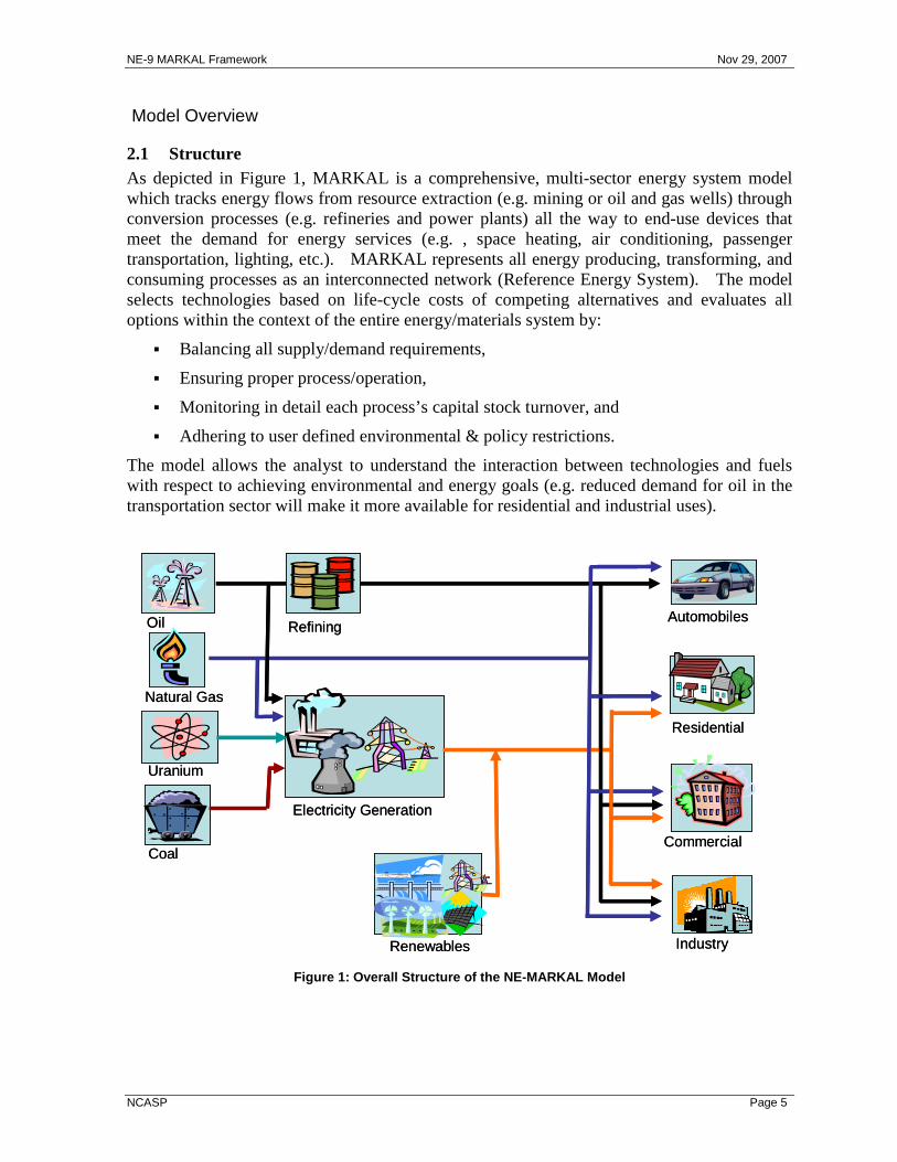
2.1 Structure As depicted in Figure 1, MARKAL is a comprehensive, multi-sector energy system model which tracks energy flows from resource extraction (e.g. mining or oil and gas wells) through conversion processes (e.g. refineries and power plants) all the way to end-use devices that meet the demand for energy services (e.g. , space heating, air conditioning, passenger transportation, lighting, etc.). MARKAL represents all energy producing, transforming, and consuming processes as an interconnected network (Reference Energy System). The model selects technologies based on life-cycle costs of competing alternatives and evaluates all options within the context of the entire energy/materials system by:

� Balancing all supply/demand requirements,

� Ensuring proper process/operation,

� Monitoring in detail each process’s capital stock turnover, and

� Adhering to user defined environmental & policy restrictions.

The model allows the analyst to understand the interaction between technologies and fuels with respect to achieving environmental and energy goals (e.g. reduced demand for oil in the transportation sector will make it more available for residential and industrial uses).

Uranium

Natural Gas

Oil

Oil

Refining

Coal

Renewables

Electricity Generation

Industry

Industry

Commercial

Residential

Automobiles

Uranium

Natural Gas

Oil

Oil

Refining

Coal

Renewables

Electricity Generation

Industry

Industry

Commercial

Residential

Automobiles

Figure 1: Overall Structure of the NE-MARKAL Model


NCASP

As a first step in the NE-9 development process, the current 6-region model (NE-MARKAL) was successfully migrated to the more user-friendly ANSWER-based data handling platform, and this model version was labeled NE-6.

1.2 Data Sources Development of the NE-9 model was closely linked to several authoritative data sources. Foremost of these is the Energy Information Administration’s (EIA) National Energy Modeling System (NEMS) model, used to produce the Annual Energy Outlook (AEO). Technology characterizations have been extracted from NEMS, along with data on base year technology stocks, resource supply options, and the sectoral growth rates used in developing demand projections for each model region (state). Other data sources include: the State Energy Data System (SEDS), which provides final energy use for each demand sector by fuel type; Gross State Product data from the Bureau of Economic Analysis; EIA's three sectoral energy consumption surveys; and the Environmental Protection Agency's eGRID emissions database. Each of these data sources and the type of data provided are described in more detail in Table 1. The transportation sector data sources will be added in the next report after this sector has been updated and expanded for the NE-9 framework.

Table 1: NE-9 Major Data Sources (Except Transporta tion Sector)

Data Source Data Provided

NEMS Model Outputs for 2002 by Census Division

Data on demand categories, fuel types, technology characterizations, base-year stock, and sectoral growth projections

SEDS-2002 data for Division 1 and 2 states

Energy use for each demand sector by fuel type

Bureau of Economic Analysis (BEA)

2002 Gross State Product (GSP)

By NAICS code

GSP shares for commercial and industrial sub-sectors by state

Manufacturing Energy Consumption Survey (MECS)

End-use energy shares by sub-sector and fuel type by census division

Commercial Building Energy Consumption Survey (CBECS)

Residential Energy Consumption Survey (RECS)

Annual Energy Outlook 2006 (AEO2006)

Current and projected final energy use and prices by sector and fuel type

Emissions & Generation Resource Integrated Database (eGRID)

Emissions rates for existing power plants

2.3 Development Status Special purpose utility programs were utilized for extracting datasets directly from NEMS for


NCASP

the electric generation, commercial and residential sectors. The fossil resource supply and industry sectors were also developed from NEMS data, but the “smart” workbook was developed in the traditional manner.

For the power sector, the utility depicts each individual power plant in a state above 25MW. Plants under 25 MW are aggregated into state-specific “small” technology characterizations based on weighted averages by fuel and technology type and vintage. Technology characterizations for existing electricity and merchant CHP plants have been developed, including heat rates, operating costs, and emissions factors. Technology options for new builds have been developed from NEMS input assumption data.

The utilities for the commercial and residential sectors extract data from Annual Energy Outlook 2006 (AEO2006) NEMS sector modules and the EIA Commercial Building Energy Consumption Survey (CBECS) and Residential Energy Consumption Survey (RECS), respectively. This information is then cross-referenced with the sectoral consumption data available from the EIA State Energy Data Summary (SEDS) to disaggregate the regional characterizations down the necessary state level. Projections from AEO2006 are used as a guide for calibration in these sectors.

For NE-9 industry sector, the data development methodology expanded the approach used to develop the current 6-state industrial representation. New and updated data sources were used to develop an approach to state-level modeling of the industrial sector using a combination of NEMS data at the regional level, Manufacturing Energy Consumption Survey (MECS) data on end-use application fuel shares, and state industrial output data from the Bureau of Economic Analysis. Industrial "captive" CHP plants are also modeled in the industrial sector, using similar data. The new approach to characterization of state-level industry sectors has proven to be robust, and in the next phase, the IRG team will consider automating the process with an extraction/processing utility.

The transportation sector from NE-6 has been migrated to the NE-9 model and loaded. Base year technology stocks and demand projections have been developed for the new states and updated for the original NE-6 states from state-level, FTA, and DOE data.

Fossil and nuclear supply options are based on EIA and NEMS data. Renewable resource and technology data for the NE-6 states has been migrated to the NE-9 model, and data has been developed for the remaining 12 states in collaboration with NREL. In addition, updated data from the IPM RGGI analysis was incorporated for some state-level renewable energy resources limits, technology characterizations and state policies.

All sectors have been successfully integrated, although calibration work remains in the transportation sector. The model has been extensively run and tested. Model projections have been evaluated against historical data and AEO006 Reference Scenario projections for the two NEMS regions.

The model has also been run as part of the Renewable Energy and Efficiency Modeling Analysis Partnership (REMAP) renewable portfolio standard analysis. Participation in this model comparison project has been and should continue to be a good test of the NE9 model in general and renewables characterization in particular.


NCASP

3. Commercial Sector Modeling

The NE-9 Commercial sector demands were based on the 14 Commercial Demand Sub-sectors in NEMS and their correlation to the categories of commercial energy use found in the AEO are shown in Table 2.

Table 2: Mapping of NE9 Commercial Demand Sub-secto rs to AEO Energy Use Categories

Name Description Includes the following AOE Demand Categories

CCK Commercial Cooking Cooking

CDG Commercial Distributed Generation Distributed Generation

CLT Commercial Lighting Lighting

COE Commercial Office Equipment Office Equipment (PC and non-PC)

COT Commercial Other/Non-Building Other Uses and Non-Building Uses (an adratio constraint will be used to tie the fuel consumption mix to AEO levels)

CRF Commercial Refrigeration Refrigeration

CSC Commercial Cooling Space Cooling

CSH Commercial Heating Space Heating

CVT Commercial Ventilation Ventilation

CWH Commercial Water Heating Water Heating

3.1 Data Development Process The overall flow of data from sources to model inputs is shown in Figure 2 and described in more detail below.

3.1.1 Base Year Demands and Residual Technology Stock The base year demands are developed using a combination of NEMS Census division-level and SEDS state-level data for the year 2002. SEDS provides final energy consumption by fuel for the entire commercial sector for each state. The NEMS data is used to create shares to break out the proportion of each fuel's final consumption going to each end use demand. These shares are then applied to the SEDS data to get final consumption by end use for each state.

To convert to useful energy, or demands, final energy consumption must be multiplied by the stock average efficiency. Base year market share data from NEMS at the Census division level is used to create efficiency-weighted shares for each residual technology, by fuel type. When these shares are multiplied by the state-level final consumption and the efficiency, the result is the portion of the demand met by each technology. These are summed to derive the total state demand. They are also divided by the capacity factor to derive the residual technology stock (RESIDs).

3.1.2 Demand Projections and User Constraints For the Commercial sector, the drivers for service demand growth over the model horizon can be “mined” from the NEMS regional commercial information available from EIA2. These 2 Projected Service Demands are derived from Input File KTech.wk1 and Output File KSDOut.txt


NCASP

census division files are cross-referenced and allocated by state according to the SEDS data.

In each demand category, user constraints (UCs) are imposed to limit the rate at which fuel switching can happen and advanced, high efficiency devices can penetrate. In some demand categories, such as refrigeration and ventilation, where technology choice is constrained by building types not represented in NE-MARKAL or other considerations, UCs are also used to limit switching between technology types. UCs are based on the base year share for the relevant fuel/technology type, and are allowed to relax by a user-specified amount over the model horizon.

Data for 14 demand categories (and 11 fuel types) consolidated

to 10 demand categories for Divisions 1 and 2

NEMS Commercial Model Outputs for 2002

by Census Division

2002 state energy consumption amounts calculated using SEDS data and NEMS end-use shares

2002 Useful demand amounts technology data and RESID capacity for end-use devices

Demand Projections

Energy use shares for each demand category and fuel type

NEMS service demand projections to 2030 for each commercial

energy use by Census Division

Weighted-average end-use efficiency calculated from NEMS

data on device efficiency and device demand shares

Technology Characterization

Data


(Table S-5)

Demand Driver for Commercial Energy Consumption applied to the Base year service demand

Data for 14 demand categories (and 11 fuel types) consolidated

to 10 demand categories for Divisions 1 and 2

NEMS Commercial Model Outputs for 2002

by Census Division



Demand Projections


NEMS service demand projections to 2030 for each commercial

energy use by Census Division




Data


(Table S-5)

Demand Driver for Commercial Energy Consumption applied to the Base year service demand

Figure 2: Data Sources and Processing for NE-9 Comm ercial Sector

3.1.3 Technology Characterizations Commercial sector technology data for parameters START, LIFE, EFF, INVCOST, and FIXOM are derived from the NEMS ktech file technology characterizations at the appropriate Census division level. An extraction utility was used to automatically process this information into a model-ready format and to make data updates and extension of the model to additional states much simpler. CF data is derived from the NEMS commercial model input filekcapfac.txt, which provides capacity factors by end use, building type, and region. NEMS service demands were used to weight them up over building types.


NCASP

4. Residential Sector Modeling

The NE-9 Residential sector demands were directly based on the 15 residential demand sub-sectors in NEMS and AEO as shown in Table 3.

Table 3: Mapping of NE9 Residential Demand Sub-sect ors to AEO Energy Use Categories

Name Description Includes the following AOE Demand Categories

RSH Residential Heating Space heating

RSC Residential Cooling Space cooling

RCW Residential Clothes Washers Clothes Washers

RDW Residential Dish Washers Dish Washers

RWH Residential Water Heating Water Heating

RCK Residential Cooking Cooking

RCD Residential Clothes Dryers Drying

RRF Residential Refrigeration Refrigeration

RFZ Residential Freezing Freezing

RLT Residential Lighting Lighting

RPC Residential Personal Computers Personal Computers

RTV Residential Television Television

RFF Residential Furnace Fans Furnace Fans

ROA Residential Other Appliances Other Appliances

RSS Residential Secondary Heating Secondary Heating


NCASP

4.1 Data Development Process The overall flow of data from sources to model inputs is shown in Figure 23 and described in more detail below.

Data for 15 demand categories (and 11 fuel types) for Census

Divisions 1 and 2

NEMS Residential Model Outputs for 2002

by Census Division



Demand Projection


NEMS energy use and device unit projections to 2030 for 15

residential demands by Census Division




Data


(Table S-4)

Calculate Demand Driver for Commercial Energy Consumption

from End-Use Energy Growth

Data for 15 demand categories (and 11 fuel types) for Census

Divisions 1 and 2

NEMS Residential Model Outputs for 2002

by Census Division



Demand Projection


NEMS energy use and device unit projections to 2030 for 15

residential demands by Census Division




Data


(Table S-4)

Calculate Demand Driver for Commercial Energy Consumption

from End-Use Energy Growth

Figure 3: Data Sources and Processing for NE-9 for Residential Sector

4.1.1 Base Year Demands and Residual Technology Stock Base year demands and RESIDs have been calculated using the same procedures as in the commercial sector.

4.1.2 Demand Projections and User Constraints For the residential sector, the NEMS modeling approach is different than in the commercial sector, and the regional information files do not contain drivers for service demand growth. NEMS does provide information on final energy demand growth and number of end-use device units. In order to derive service demand drivers from this information, the average device energy consumption was calculated. For most demands, NEMS reports a decreasing unit energy consumption because of gradual end-use device efficiency improvement. However, the rate and manner of device efficiency improvement is to be investigated using the NE-9 model. Therefore, for most residential sub-sectors, service demand drivers were developed by using the base year average device energy consumption multiplied by the projected device population. For some sub-sector demands, especially lighting, personal computers, and miscellaneous energy demands, the average device energy consumption


NCASP

increases over time, and for those sub-sectors, the projected device energy consumption from NEMS was used to develop the demand drivers. These census division files are cross-referenced and allocated by state according to the SEDS data.

As in the commercial sector, initial fuel and technology type shares for each service demand are also derived from this data and used to construct user constraints that limit the rate at which switching can happen for each residential sector demand.

4.1.3 Technology Characterizations Technology characterizations for the residential sector were developed using the same procedures as in the commercial sector.

5. Industrial Sector Modeling

For the NE-9 framework, the recommended approach to modeling Industrial sector energy use follows the approach used to model the industrial sector energy use for NE-MARKAL in that all industry demands are mapped into general end-use categories of steam boilers, process heat, machine drive, electro-chemical, feedstock and other uses using MECS data. The end-use technologies supplying each of the end-use categories are defined by fuel type and are tied together by ADRATIOs that start at the current fuel share but relax over time to allow fuel switching to occur. However, there are some differences. In particular, all the energy demands are in units of trillion BTUs. Although NEMS does provide physical output quantities for aluminum, cement, glass, paper and steel, it is not clear that there is value in defining these demands in these units.

5.1 Data Development Process

5.1.1 Base Year Demands and Residual Technology Stock The NEMS Industrial Model provides breakouts of energy use for 15 industry sub-sectors and refineries for the 4 Census regions5 by fuel type. For NE-9, these 15 industry sub-sectors were consolidated into 6 sub-sectors as shown in Table 4. Each industry sub-sector had demands in most or all of the end-use demands as also shown in Table 4.

Table 4: List of NE9 Industrial Sub-sectors and End -use Demands

Industry Sub-sectors End-use Demands*

Chemical Steam

Paper Process heat

Metals Electrochemical

Glass-Cement Mechanical drive

Durables Feedstock

Other Other

* Not all demands in all Sub-sectors

5 Northeast, South, Midwest and West.


NCASP

Figure 4 describes the process used to build up the industrial final energy use, base-year service demands and residual capacities. The data development for NE-9 started with the NEMS final energy consumption data for the Northeast region as detailed in the NEMS regional industrial tables6 for 2002. This file provides fuel use data for each industry sector broken down into buildings, processes, steam/cogeneration and electricity generation. This data was collected into a subset of fuel categories that more closely matched the SEDS data and that will be more appropriate for model use.

This regional table of industrial energy consumption by fuel type was separated into state shares of industrial energy use using the data from the Bureau of Economic Analysis (BEA), which provides Gross State Product (GSP) data for a large number of industries by NAICS code. The 2002 GSP data, available from the BEA - Regional Economic Accounts7, was used to determine state shares of energy use for each industry sector based on the assumption that industrial energy use is proportional to industrial economic output.

The NEMS industry categories were mapped by their NAICS codes to match the NAICS codes used in the BEA breakdown. For now we have used the BEA breakdown, but some disaggregation may be desired at a future date. For example, BEA only reports primary metals manufacturing (331), which included both steel and aluminum.

Next, the state-level industry sector energy use shares - obtained by applying the state industry GSP shares to the regional industry sector values - were calibrated to the final energy use numbers provided in the SEDS industrial sector energy consumption table. The workbook had been initially developed using the SEDS 2001 data, but it has now been updated to use the recently released SEDS 2002 data8.

MECS data9, which provides national-average end use energy consumption by end-use type for a variety of industries by NAICS code, was used to develop end-use shares for each industry sub-sector and fuel type for the applications of boiler steam, CHP, process heat, machine drive, electrochemical process and other uses. These shares were applied by state-level industry sector energy use to get base year final energy use by state, industry sector, fuel type and end-use. The base-year final energy data then was then used to determine the RESID capacity for each state, industry sector, end-use application and fuel type.

6 See file: NEMS Industry_regional.xls 7 See http://www.bea.gov/bea/regional/gsp/ 8 SEDS Table S6: Industrial Sector Energy Consumption Estimates, 2002. 9 MECS Table 5.2: End Uses of Fuel Consumption within NAICS Codes, 2002.


NCASP

Northeast Regional Energy Use by Fuel and 15

Industry sectors

NEMS Industrial Model Outputs for 2002

by 4 Census Regions

Calibrate State Industrial Energy Use

using SEDS Industrial Fuel Use Data

SEDS 2002 DataTable S6

Calculate State Shares of Industry Energy Use using

GSP shares

Selection of Major Industry Sectors and End-

Use Processes

Use MECS Data toDetermine Industrial

Energy Use byEnd-Use Process

Demand Projection

Bureau of Economic Analysis (BEA) Gross State Product (GSP)by Industry Sector for 2002

Combine 15 industry sectors to match BEA-GSP

Industry categories

Calculate RESID capacity for Industrial End-Use

Processes

MECS Industrial Energy use by Industry Sector and End-Use

Calculate Base Year Energy Consumption for

Industrial End-Use Processes

Technology Data (Efficiency, capacity factor, etc.)

Model Inputs

Northeast Regional Energy Use by Fuel and 15

Industry sectors

NEMS Industrial Model Outputs for 2002

by 4 Census Regions

Calibrate State Industrial Energy Use

using SEDS Industrial Fuel Use Data

SEDS 2002 DataTable S6

Calculate State Shares of Industry Energy Use using

GSP shares

Selection of Major Industry Sectors and End-

Use Processes

Use MECS Data toDetermine Industrial

Energy Use byEnd-Use Process

Demand Projection

Bureau of Economic Analysis (BEA) Gross State Product (GSP)by Industry Sector for 2002

Combine 15 industry sectors to match BEA-GSP

Industry categories

Calculate RESID capacity for Industrial End-Use

Processes

MECS Industrial Energy use by Industry Sector and End-Use

Calculate Base Year Energy Consumption for

Industrial End-Use Processes

Technology Data (Efficiency, capacity factor, etc.)

Model Inputs

Figure 4: Data Sources and processing for NE-9 Indu strial Sector

5.1.2 Demand Projections Future projections of the industrial energy demands were based on the 2006 NEMS Industrial Model final energy consumption projections for the Northeast, which go to 2030. These final energy consumption projections already incorporate the EIA projected efficiency improvements of industrial energy consumption for both manufacturing and non-manufacturing sectors.

5.1.3 Technology Characterizations O&M costs for existing technologies and both capital costs and O&M costs for new technologies were derived from the SAGE technology characterization database. The year 2000 dollars were converted to 2002 dollars using the GDP deflator from the Bureau of Economic Analysis.

Technology characterizations for industrial CHP plants have similarly been drawn from SAGE. See Section 6 for more details on CHP modeling.


NCASP

6. Electricity Generation and CHP

6.1 Overview and Modeling Issues For electricity only plants, the NE-9 modeling approach is to represent individual plants down to a minimum size threshold, and aggregated "small" plants below the threshold. Data is taken from EIA reports, NEMS, and eGRID.

For combined heat and power (CHP) plants, there are two types of CHP applications that need to be considered. The first is independent or merchant CHP plants that primarily sell electricity to the grid and are not integrated into industrial processes. The heat (usually steam) they produce can be used in a range of low to medium temperature applications including district heating, greenhouses or industrial manufacturing. These plants are modeled in the electricity sector in the same manner as the electricity generation technologies.

The second class of plants is industry CHP plants that are more tightly integrated with the industrial processes they serve and often (but not always) use by-product fuels from industrial processing. The fuel consumption and residual capacity of these plants (and on-site generation) have been extracted from the NEMS industrial database and apportioned to the states according the SEDS data, just like the other industrial energy consumption data. The CHP end-use shares are derived from the MECS data, and specific CHP technologies are defined according to the fuel input. Technology characteristics are derived from the SAGE industrial technology database. An example RES for Industrial Chemical Processes is shown in Figure 5.

NE-12 MARKAL Framework July 15, 2007

International Resources Group

Chemical Steam Demand

(ICSTM)

Chemical Process Heat Demand

(ICPRH)

Chemical Electrochemical Demand (ICECH)

Chemical Feedstock Demand

(ICFST)

Chemical Other Demand

(ICOTH)

Fuel shares for Steam, Process Heat, Machine Drive, Feedstock and Other are tied by

Adratios that relax over time.

LPG

Distillate Oil

Natural gas

Electricity

Coal

Other PetroleumProducts

.

.

.

Natural gas

Petrochemicals

LPG

Electricity

LPG

Distillate Oil

Natural gas

Electricity

.

.

.

Gasoline

Distillate OilBoilers

Natural gasBoilers

Coal Boilers

BiomassBoilers

Residual OilBoilers

CHPBoilers

.

.

.

Chemical IndCHP Plants(ICCHPxxx)

INDELC

LTH to ChemicalIndustry

LTH from CPD Plants

ICLTH

ELC to Industry

ELC from Grid

INDELC

On-site Generation

(IExxx)

INDELC

ICLTH

Chemical IndustryProcess Improvement-1

(Conservation Tech)

ICSTMICPRHICOTH


(Conservation Tech)

ICFSTICECH

Chemical Machine Dive

Demand (Not detailed) (ICMDR)

Chemical Steam Demand

(ICSTM)

Chemical Process Heat Demand

(ICPRH)

Chemical Electrochemical Demand (ICECH)

Chemical Feedstock Demand

(ICFST)

Chemical Other Demand

(ICOTH)

Fuel shares for Steam, Process Heat, Machine Drive, Feedstock and Other are tied by

Adratios that relax over time.

LPG

Distillate Oil

Natural gas

Electricity

Coal


.

.

.

LPG

Distillate Oil

Natural gas

Electricity

Coal


.

.

.

Natural gas

Petrochemicals

LPG

Natural gas

Petrochemicals

LPG

Electricity

LPG

Distillate Oil

Natural gas

Electricity

.

.

.

Gasoline

LPG

Distillate Oil

Natural gas

Electricity

.

.

.

Gasoline


Natural gasBoilers

Coal Boilers

BiomassBoilers

Residual OilBoilers

CHPBoilers

.

.

.


Natural gasBoilers

Coal Boilers

BiomassBoilers

Residual OilBoilers

CHPBoilers

.

.

.

Chemical IndCHP Plants(ICCHPxxx)

INDELC


LTH from CPD Plants



LTH from CPD Plants

ICLTH

ELC to Industry

ELC from Grid

INDELCELC to IndustryELC to Industry

ELC from Grid

INDELC

On-site Generation

(IExxx)

INDELCOn-site

Generation(IExxx)

INDELC

ICLTH


(Conservation Tech)

ICSTMICPRHICOTH


(Conservation Tech)

ICFSTICECH

Chemical Machine Dive

Demand (Not detailed) (ICMDR)

Figure 5: Example RES for Industrial Chemical Proce ss Energy Use and CHP

NE-12 MARKAL Framework


The important CHP modeling issue is to ensure that electricity and low-temperature heat (LTH) from the independent CHP plants can be accessed by the industrial demand sub-sectors, and that the electricity and LTH generated in the industrial CHP plants is accessible – within reasonable limits – to non-industry demands. For electricity these limits are quite minimal as electricity can be transmitted long distances over the grid. In NE-9, the independent CHP plants sell to the general grid that is available to all demand sectors. The industrial CHP plants sell to the grid that supplies electricity to the industrial demands.

For the LTH demands there is a much smaller range within which this energy can reasonably be transmitted, and so significant constraints exist that are largely based on proximity requirements. In the industrial sector, it is primarily the steam demands that are open to outside supply of LTH. Likewise, it is primarily industry generated steam that is available to supply non-industry LTH loads.

Currently, the option for independent CHP plants to provide LTH demands to industry is modeled using the 2002 NEMS industrial model data, which is used to calculate the current ratio of CHP heat use to total steam heat by region and by industry sub-sector. This provided the starting bound for sub-sector based ADRATIOs. The selection of future bounds for the sub-sector based CHP activity is determined by setting the upper bound as a percentage increase over the current ratio of CHP heat to total steam heat. The percentage increase is a variable parameter in the ANSWER loadsheet, so that scenarios can be easily created.

Furthermore, the non-industrial LTH demand is not modeled because NEMS data indicated it is quite small and not expected to grow. However, the option for commercial sector CHP plants and for industry to provide LTH to the commercial sector can be added to the model in the future to support policy analyses in this area.

6.2 Data development process

6.2.1 Existing Plants The data sources for existing electricity and independent CHP generation technologies are EIA Forms 860 (existing and planned units), 767, 759/906 and Form 1 which collectively list generating unit capacity, prime mover, fuel sources, location, plant operation and equipment design (including environmental controls), fuel consumption and quality and for the larger investor-owned plants the non-fuel operating costs. Each survey form has its own universe of units covered. All units are covered by one or more of the forms.

A data mining utility has been developed to convert this data to ANSWER "Smart" upload templates. Because these forms list every plant regardless of size, small plants must be aggregated to an appropriate level to obtain a manageable number of technologies that still adequately represents the diversity of existing plants and their differential use in the system. All existing generation units above a specified capacity threshold are represented as individual technologies, retaining all unit-specific information. This threshold is currently set at 25MW, but can be adjusted to obtain the desired level of detail in the sector.

Plants below the capacity threshold have been aggregated using the following characteristics11 11 Note that ECP designations separate coal units with and without scrubbers and by vintage. In addition, for coal units, the coal supply region providing the fuel input was used to further distinguish between units for aggregation purposes.



to define a plant type:

• fuel input type • plant type (taken from the Electricity Capacity Planning (ECP) designations in NEMS) • State/Region

For each grouping of aggregated plants, data for the representative MARKAL technology is derived by calculated a capacity weighted average of selected fields from the EIA forms and totaling other fields. The following fields have been averaged:

• heatrate • annual cap additions (added to fixed O&M costs) • fixed O&M • variable O&M • capacity factor • availability • scrubber efficiency • NOx emission rate.

The following fields have been totaled:

• total of summer capacity • total of winter capacity (used by adjusting the AF by season)

6.2.2 New Fossil and Nuclear Plants Technology characterizations for new fossil and nuclear plant options are drawn from NEMS.

6.2.3 New Renewable Plants Technology characterizations and resource availability for new renewable plants are described in Section 6.3.

6.2.4 Emissions

Emissions rates for NOx, SOx, and Hg for all existing technologies are mined from EPA's eGRID database. The eGRID database provides emissions rates at the plant level, whereas NE-12 technologies are represented at the unit level. Since a single plant may consist of several units that may burn different fuels and have greatly dissimilar emissions rates, assigning eGRID rates to the NE-9 existing technologies has been challenging. Calibration and testing will be necessary to determine if the current procedure is sufficient or if further development is needed.

Because coal markets are constrained by many non-economic factors that cannot be modeled in NE-9, existing coal plants are constrained to their current coal source (Appalachian, Western, or imports.) Their historical emissions rates are applied throughout the model horizon. A scrubber retrofit option for plants that currently lack them is under development.

All new coal plants are assumed to be built with scrubbers. Their SOx and Hg emissions rates are based on the S and Hg content of the coal burned and scrubber removal rates. These plants are free to choose coal type. Scrubber removal rates and NOx emissions rates for all new plants are derived from NEMS.



6.3 Electricity trade Electricity trade in the model is represented by two constraints: 1) bilateral trade constraints and 2) joint constaints. Bilateral constraints represent the capacity transfer limit between two states. Joint constraints establish limits on the simultaneous flows into or out of a state. The joint and bi-lateral constraints represent the grid reliability and security concerns that need to be managed by the grid operators. The data to establish these limits were compiled by OnLocation, Inc. from "Assumption Development Document: Regional Greenhouse Gas Initiative Analysis", ICF Consulting, February 10, 2005.

The constraints used in the model represent the existing grid capability. One of the more difficult challenges is to ascertain the costs associated with increasing these limits. Because of the integrated nature of the grid and the limited ability to direct flows across specific paths, the cost of adding a new transmission line rarely represents the cost of increasing the transfer limits between two sections of a grid, e.g., two states. Periodically, the NERC performs a series of load flow studies to establish the impacts on the grid of significant new transmission facilities and may represent a potential source for this type of data. While there are selected transmission corridors that could get upgraded over the model horizon, we have no source of data that describes the costs or resultant increased transfer limits. As such, for the reference analyses, the model is not currently allowed to increase the transfer limits.12

Two areas regarding electricity trade in the NE9 model need additional attention. The first is the treatment of potential flows from and to outside the 9 states being modeled. This is particularly important for states like Pennsylvania which are situated between the relatively low cost electricity producing areas of Kentucky and Ohio and the high cost areas of New Jersey, Connecticut and New York. Considerable amounts of power flow into and out of Pennsylvania and a more complete approach to dealing with this issue is needed.

The second related area is the treatment of Canadian imports and exports. New York in particular is impacted by the power markets in Ontario and Quebec (as is other parts of New England). Again, a more complete approach is warranted to address these regions. This is particularly important if NESCAUM or the states want to understand the dynamics between various energy and climate policies as they are impacted by international leakage or trade.

7. Resource Supply, Trade, and Upstream

7.1 Fossil Fuels There is no indigenous fossil resource in New England, and so in NE-MARKAL a single fixed-price resource cost - taken from AEO2005 was used. Possible resource extraction (MIN) processes were given a zero upper bound.

As the model was expanded to the Northeast states, there are some indigenous resource supplies (particularly coal). However, it was decided that the NE-MARKAL approach should

12 It should be recognized that current transmission limits or constraints can be addressed by both adding new transmission facilities and by adding generating capacity on the constrained side of the interface. Since the model is assumed to be building new facilities to meet increasing demands and replace retiring units, for modeling purposes it is assumed these new facilities will be situated to relieve any known transmission constraint.



be continued, since the influence of regional policy on national market prices will continue to be minimal. In principle, coal production supply curves could be drawn from NEMS supply curves for the Northern Appalachian region and apportioned to the state level. However, coal is traded nationally based on price, as well a short and long-term contracts. Representing this trade would require tight user constraints to fix the ratio of in-region production consumed versus exported, increasing model complexity without adding meaningful analysis options.

Accordingly, the region is modeled as a price taker. Imports of fossil resources and refined petroleum products are available in unlimited amounts at AEO2006 reference case sector delivered prices13. This approach has the drawback of permitting unlimited fuel switching with no cost penalty

Available coal types have been simplified from the forty-plus types NEMS tracks to Appalachian, Western, and imported. Sulfur content is taken from the NEMS EMM database, and weighted averages for NE-9 coal types calculated using 2002 coal consumption by NEMS type. (Mercury content will be calculated in a similar manner.) Carbon emissions14 for all fuels are tracked by sector based on the carbon content of fuels.

7.2 Other Fuels Cost curves for delivery of centralized and decentralized hydrogen are taken from an Argonne National Lab report.15 Nuclear fuel costs are taken from NEMS.

7.3 Renewables Renewable resources are indigenous to each state, and supply data for renewables has been modeled in the same manner as was developed for NE-MARKAL.

7.3.1 Wind Resources

The National Renewable Energy Lab (NREL) provided N ESCAUM with wind potentials for on-shore and off-shore resources and as a function of wind class (3 through 7) and distance from grid transmission lines. NREL processed their standard state-level w ind resource maps and transmission line data from

PowerMap 16 for lines between 69 - 345 kV buffered to identify raw wind resource potential for 0-5, 5-10, 10-20, and >20 mile distance bands. The standard envi ronmental, land use and other exclusion criteria we re

then applied to the data to produce a developable r esource potential. These criteria are provided in

Table 5.

13 AEO2006 Supplemental Tables 11 and 12 and PMMRPT file. 14 Carbon emission factor data from EIA, Emissions of Greenhouse Gases in the United States 2002, Report #: DOE/EIA-0573(2002). 15 Hydrogen Demand, Production, and Cost by Region to 2050, Argonne National Laboratory and TA Engineering, ANL/ESD/05-2. 16 Platts - Dec 2006 update.



Table 5: Criteria for Defining Available Windy Land (numbered in the order they are applied):

Environmental Criteria Data/Comments:

2) 100% exclusion of National Park Service and Fish and Wildlife Service managed lands

USGS Federal and Indian Lands shapefile, Jan 2005

3) 100% exclusion of federal lands designated as park, wilderness, wilderness study area, national monument, national battlefield, recreation area, national conservation area, wildlife refuge, wildlife area, wild and scenic river or inventoried roadless area.


4) 100% exclusion of state and private lands equivalent to criteria 2 and 3, where GIS data is available.

State/GAP land stewardship data management status 1, from Conservation Biology Institute Protected Lands database, 2004

8) 50% exclusion of remaining USDA Forest Service (FS) lands (incl. National Grasslands)


9) 50% exclusion of remaining Dept. of Defense lands USGS Federal and Indian Lands shapefile, Jan 2005

10) 50% exclusion of state forest land, where GIS data is available

State/GAP land stewardship data management status 2, from Conservation Biology Institute Protected Lands database, 2004

Land Use Criteria

5) 100% exclusion of airfields, urban, wetland and water areas.

USGS North America Land Use Land Cover (LULC), version 2.0, 1993; ESRI airports and airfields (2003)

11) 50% exclusion of non-ridgecrest forest Ridge-crest areas defined using a terrain definition script, overlaid with USGS LULC data screened for the forest categories.

Other Criteria

1) Exclude areas of slope > 20% Derived from elevation data used in the wind resource model.

6) 100% exclude 3 km surrounding criteria 2-5 (except water) Merged datasets and buffer 3 km

7) Exclude resource areas that do not meet a density of 5 km2 of class 3 or better resource within the surrounding 100 km2 area.

Focalsum function of class 3+ areas (not applied to 1987 PNL resource data)

Note - 50% exclusions are not cumulative. If an area is non-ridgecrest forest on FS land, it is just excluded at the 50% level one time.

This developable wind resource data was converted into state-level upper resource bounds for 8 distinct wind technologies. These technologies and some indicative data are shown in Table 6. Onshore-1 corresponds to less than 20 miles to a 68 kV or higher transmission line, and the cost of this technology were based on a recent assessment of wind farm costs compiled by Navigant Consulting17 and used in the RGGI IPM analysis. Onshore-2 corresponds to greater than 20 miles to a high voltage transmission line and imposes and

17 ”New Jersey Renewable Energy Market Assessment,” Navigant Consulting, August 2004.



incremental investment cost on the wind technology based on the transmission line cost for an average 50 mile line length. Offshore-1 corresponds to 5 to 20 nm from shore (Note, there is a 100% exclusion for 0 to 5 nm from shore), and Offshore-2 corresponds to 20 to 100 nm from shore. The investment cost for the Offshore-2 wind technologies also contains an incremental transmission line cost.

Table 6: Wind Resource Data

No. Type Wind Class

Base Year Investment

Cost Resource Upper Bound in 2020 (MW)

CT MA ME NH RI VT NJ NY PA

1 Onshore -1 4-5 1268 51 570 1,710 587 30 1,374 83 1,553 970

2 Onshore -1 6-7 1532 0 123 720 149 0 0 0 30 1

3 Onshore -2 4-5 1268 0 32 716 117 0 366 0 121 38

4 Onshore -2 6-7 1532 0 10 193 16 0 0 0 1.4 0

5 Offshore -1 4-5 2006 223 717 793 173 304 0 2,791 5,282 980

6 Offshore -1 6-7 2270 0 0 0 0 0 0 68 39 0

7 Offshore -2 4-5 2006 0 10,612 8,647 194 1,345 0 2,065 4,377 0

8 Offshore -2 6-7 2270 0 48,733 9,142 103 3,823 0 21,715 19,470 0

Capacity factor data for each wind technology was derived at the census division level from NEMS data and used for each at the state level. Growth constraints of 10% per year and hurdle rates of 25% were added to represent siting, financing, and other considerations expected to slow penetration of wind in the reference case. These may need to be relaxed or reconsidered in policy analysis cases.

7.3.2 PV Capacity Factors For solar photovoltaic (PV) systems, the technical potential of the resource is tremendous and does not provide a meaningful limit on the amount of resource that can be used. The capacity factor for PV systems is the most meaningful parameter impacting performance. These were provided by NREL for each day/season time slice, and are shown in Table 7 for central PV systems for grid electricity generation. This technology was assumed to use one-axis tracking. Two other PV technologies were developed – for residential rooftops and commercial rooftops – and have capacity factors based on a fixed tilt orientation.

Table 7: Capacity Factors for Central Solar PV Syst ems

Region AF(Z)(Y)~ID AF(Z)(Y)~IN AF(Z)(Y)~SD AF(Z)(Y) ~SN AF(Z)(Y)~WD AF(Z)(Y)~WN

CT 0.333 0.000 0.423 0.000 0.219 0.000

MA 0.340 0.000 0.443 0.001 0.224 0.000

ME 0.345 0.000 0.444 0.001 0.234 0.000

NH 0.333 0.000 0.434 0.001 0.232 0.000

RI 0.341 0.000 0.454 0.000 0.223 0.000

VT 0.322 0.000 0.437 0.001 0.200 0.000



NJ 0.334 0.001 0.411 0.008 0.226 0.000

NY 0.316 0.002 0.418 0.011 0.205 0.000

PA 0.329 0.003 0.415 0.011 0.209 0.000

The principal constraint on PV systems is the growth rate that the industry can sustain over time. Thus, each PV technology contains an annual growth rate constraint. Based on historical growth rates, these were set at 10%, 20% and 30% respectively for central, commercial and residential PV technologies.

7.3.3 Biomass Resources Oak Ridge National Lab (ORNL) has estimated the availability and delivered price of six types of biomass resources for the US18. For agricultural residues, the delivered price includes the cost of collecting the residues, the premium paid to farmers to encourage participation, and transportation costs.

The workbook, NE-9 Markal Biomass Resource Data-tBTU.xls, contains the basic quality estimates in dry tons per year, applies availability estimates for each category as estimated by ORNL, and uses the lower heating value for each biomass type to determine the resource potential for each state. Woody biomass and agricultural wastes were combined as one aggregated biomass resource, as the technology differences for application of these two biomass types are not great.

Four biomass resource supply steps were developed for each state, corresponding to each price step in the ORNL data. The first three price steps start in 2002, as they correspond to existing supplies of forest and urban wood waste residues. The final step corresponds to energy crops, which ORNL assumed are available by 2010. The final step was constructed such that half the potential energy crop supply is available in 2008, and the full energy crop potential is available in 2011.

The resulting aggregated biomass resources by state are shown in the Table 8. For the initial NE-9 states, the biomass resource available at each price step is plotted in Figure 6. It can be seen that significant both PA and NY contain significant biomass resource potential compared to the other nine states. (Ohio, which is being modeled under a separate modeling effort, represents another significant increase in biomass resource potential.)

Table 8: NE-9 Biomass Resource Supply (tBTU/yr) at Four Cost Levels- Yr 2002 dollars

Cost (M$/tBTU) 1.54 2.31 3.39 4.26

Connecticut 2.95 4.96 4.98 7.48

Maine 1.30 2.49 2.63 2.81

Massachusetts 5.00 8.42 8.45 11.42

New Hampshire 1.32 2.40 2.45 4.60

Rhode Island 0.36 0.60 0.60 0.67

18 Biomass Feedstock Availability in the United States: 1999 State Level Analysis, Marie E. Walsh, Robert L. Perlack, Anthony Turhollow, Daniel de la Torre Ugarte, Denny A. Becker, Robin L. Grahama, Stephen E. Slinsky, and Daryll E. Ray (updated January 2000).



Vermont 0.49 0.92 0.96 5.15

Delaware 0.46 0.78 2.59 7.34

Maryland 2.44 4.14 9.75 24.35

New Jersey 4.64 7.76 8.44 10.23

New York 13.61 23.11 25.91 68.23

Ohio 8.88 14.89 218.35 290.91

Pennsylvania 4.81 8.42 12.62 59.02

Most of the increase at $50/dry ton is due to energy crops, which the ORNL data assumes is all switchgrass, because of its higher productivity. However, this may not be the best assumption for the six New England states. The ORNL methodology assumes that agricultural lands are used for energy crops, and it factors in competition between food production and energy crops. It discounts marginal or unused lands, such as interstate highway medians, which are not traditional crop lands. Therefore, this supply data underestimates the energy crop potential, especially for New England, which does not have a lot of surplus agricultural land, but does have marginal lands suited for poplar and other energy crops. This issue should be addressed at a future date.

This biomass resource, as estimated by ORNL, was unable to meet base year consumption of biomass in all sectors in several states, as reported in SEDS data. It is unclear why this inconsistency exists. It could be that biomass is traded across state lines. Such trade is currently unrepresented in the model. It could also be that the ORNL data does not cover residential wood consumption, but only industrial and energy generation scale use. Under this latter assumption, a separate category of biomass supply, Biomass Residential Wood, was created that is available to serve residential demand only. Growth of this demand is tightly controlled and wood does not compete meaningfully with other fuels. This resource was made available across the model horizon at twice base year consumption levels.

Review of the RGGI IPM analysis input assumptions shows an apparently different interpretation of this same ORNL data. The differences remain to be investigated.



0

20,000,000

40,000,000

60,000,000

80,000,000

100,000,000

120,000,000

140,000,000

160,000,000

180,000,000

20 30 40 50

Delivered Price ($/dry ton)

Mill

ion

BT

U/y

r

Pennsylvania

New York

New Jersey

Vermont

Rhode Island

New Hampshire

Massachusetts

Maine

Connecticut

Figure 6: Aggregated Biomass Resources for New Engl and States

7.3.4 Landfill Gas Resources Landfill gas resource availability and technology characteristics were taken from the work performed for the RGGI Working Group and Stakeholders19. The state-level potentials are provided in Table 9 and were used to develop upper bounds for the two types of landfill gas systems shown in the table. The reference also provided technology characteristics for the two technologies.

Table 9: Landfill Gas Resource Potential (MW)

State LFG – with Collection System (MW) LFG – without Collection System (MW)

2005 2010 2015 2020 2005 2010 2015 2020

CT 2.6 12 14 16.3 0 3.9 4.4 5.2

MA 4.3 19.9 23.2 27 0 4.6 5.4 6.3

ME 1.1 4.9 5.8 6.7 0 1.3 1.5 1.8

NH 2.1 9.8 11.4 13.4 0 0 0 0

RI 0.7 3.2 3.8 4.4 0 0 0 0

19 Assumption Development Document: Regional Greenhouse Gas Initiative Analysis, Prepared by ICF Consulting for Regional Greenhouse Gas Initiative (RGGI) Staff Working Group and Stakeholders, August 2006.



VT 0.1 0.3 0.4 0.4 0 5.5 6.4 7.5

NY 17.4 81 94.5 110.3 0 7.9 9.3 10.8

NJ 31.7 147.7 172.4 201.2 0 8.8 10.3 12

PA 26.7 124.6 145.3 169.6 0 3 3.5 4.1

DE 7.4 34.4 40.1 46.8 0 20.9 24.4 28.5

MD 3.6 16.7 19.5 22.8 0 0 0 0

Total 97.4 454.4 530.4 618.9 0 55.9 65.2 76.1

7.3.5 Small Hydropower Resources The resource potential for small hydropower (SHP) plants was based on a report from the SHP resource Center at Idaho National Engineering Laboratory20 and is presented in Table 10. The technology characterization data was based the range of high and low costs as reported to the RGGI Working Group and Stakeholders19.

Table 10: Small Hydropower Resource Potential (MW)

CT MA ME NH RI VT NJ NY PA

Generic Impoundment Hydropower 24.3 76.6 815.2 25.5 10.2 161.9 5.3 656.6 291.9

Generic Run-of-River Hydropower 19.1 55.7 227 6.5 1.3 11.7 4.1 651.9 410.6

7.3.6 Production Tax Credit As part of the REMAP analysis, the federal production tax credit (PTC) for wind, biomass, and landfill gas was added to the model. This provides a 10-year credit for facilities put in place by 2007 (2008 model year in NE9). Adding the PTC required triplicating the eligible technologies to track vintage for plants purchased in 2005, 2008, and 2011 or later. The PTC is presently assumed not to be renewed after 2007.

7.3.7 State Renewable Portfolio Standards Existing state renewable portfolio standards (RPS) requirements were added, as modeling by the RGGI IPM analysis, which simplified the standards to represent the percentage of generation to be met by new renewable plants. The standards are listed in Table 11.

Table 11: State RPS standards

Percentage of Load Required

State Program 2005 2010 2015 2020

CT Class 1 0.78% 6.05% 6.09% 6.12%

NJ- Class 1 Main Tier 0.00% 3.22% 5.55% 7.88%

NY- Main Tier 4.05% 6.43% 6.43%

PA - Tier 1 Main Tier 1.13% 3.02% 4.19%

MA 0.55% 2.72% 4.89% 7.06%

20 U.S. Hydropower Resource Assessment, Idaho National Engineering Laboratory, Renewable Energy Products Department, July 1995.



RI 0.00% 2.49% 7.97% 13.94%

NJ- Solar Tier (PV only) 0.01% 0.20% 0.41% 0.62%

PA - Solar Tier (PV only) 0.00% 0.01% 0.24% 0.49%

The implementation represents the standards as they are on the books, without adjustment for how they might be met or fail to be met on the ground.

8. User Constraints for Calibration

User constraints were added as needed to slow fuel and technology switching and represent real-world constraints beyond the model's scope. These include:

Demand sectors: Constraints limit fuel switching, technology type switching, and advanced technology penetration. Relaxation rates for these constraints are under user control on the respective templates.

Gas-fired generation constraints: State-level and cross-region constraints are needed to force gas plant capacity addition and operation in the absence of adequate peak representation. In the nine-plus timeslice version of the model, these constraints may be reduced or unnecessary.

Renewable penetration: Renewable technologies are often over-attractive to MARKAL because they have low or zero fuel costs. To represent siting, financing, and other factors expect to slow renewable penetration in the reference case, a hurdle rate of 25% was added to all renewable technologies. In addition, growth constraints were added for some technologies. The current values are shown in Table 12 below. (Values may change as analysis proceeds.)

Table 12: Constraints on Renewables

Technology GROWTH rate DISCRATE Comments

Hydro 1% 25% Hydro technologies are very attractive on a cost basis to MARKAL, but AEO projects almost zero

increase in hydro capacity

Wind 10% 25%

Biomass 25%

MSW, landfill gas 25%

Solar PV 10, 20, 30% 25% GROWTH rates for centraliz ed, commercial, and residential, respectively

ne-9 markal structure, data and calibration

Documents