NBER WORKING PAPER SERIES

STOCK MARKET TRADING AND MARKET CONDITIONS

John M. GriffinFederico Nardari

René M. Stulz

Working Paper 10719http://www.nber.org/papers/w10719

NATIONAL BUREAU OF ECONOMIC RESEARCH1050 Massachusetts Avenue

Cambridge, MA 02138August 2004

Griffin is an Associate Professor of Finance at the McCombs School of Business, University of Texas atAustin. Nardari is an Assistant Professor of Finance at the WP Carey School of Business, Arizona StateUniversity. Stulz is the Everett D. Reese Chair of Banking and Monetary Economics, Ohio State University,and a Research Associate at the NBER. We are very grateful to Sriram Villupuram for superb researchsupport. We thank Keith Brown, Stijn Claessens, Martijn Cremers, Enrico Perotti, Simon Potter, Laura Starks,Paul Tetlock, Sheridan Titman, Selim Topaloglu as well as seminar participants at Queen’s University, theUniversity of Amsterdam, and the University of Texas at Austin Accounting and Finance mini-conference.The views expressed herein are those of the author(s) and not necessarily those of the National Bureau ofEconomic Research.

©2004 by John M. Griffin, Federico Nardari, and René M. Stulz. All rights reserved. Short sections of text,not to exceed two paragraphs, may be quoted without explicit permission provided that full credit, including© notice, is given to the source.

Stock Market Trading and Market ConditionsJohn M. Griffin, Federico Nardari, and René M. StulzNBER Working Paper No. 10719August 2004JEL No. G1

ABSTRACT

This paper investigates the dynamic relation between market-wide trading activity and returns in 46

markets. Many stock markets exhibit a strong positive relation between turnover and past returns.

These findings stand up in the face of various controls for volatility, alternative definitions for

turnover, and differing sample periods, and are present at both the weekly and daily frequency.

However, the magnitude of this relation varies widely across markets. Several competing

explanations are examined by linking cross-country variables to the magnitude of the relation. The

relation between returns and turnover is stronger in countries with restrictions on short sales and

where stocks are highly cross-correlated; it is also stronger among individual investors than among

foreign or institutional investors. In developed economies, turnover follows past returns more

strongly in the 1980s than in the 1990s. The evidence is consistent with models of costly stock

market participation in which investors infer that their participation is more advantageous following

higher stock returns.

John M. GriffinMcCombs School of BusinessUniversity of Texasjohn.griffin@mail.utexas.edu

Federico NardariWP Carey School of BusinessArizona State Universityfederico.nardari@asu.edu

René M. StulzFisher College of BusinessOhio State University806A Fisher Hall2100 Neil AvenueColumbus, OH 43210-1144and NBERstulz@cob.osu.edu

1

It is part of market folklore that liquidity dries up following poor returns. In bear markets,

trading volume is down, brokers make less money, fewer equity issues take place, and stock

mergers become scarce. Although there is some evidence of a relation between turnover and past

returns, there is neither a comprehensive documentation of it nor a generally agreed upon

explanation for it.1 In this paper, we investigate the relation between volume and lagged returns

for 46 markets across the world using weekly data. The use of international data makes it

possible to evaluate the robustness of the relation. Further, and perhaps more importantly, we can

exploit cross-country differences in the relation to test possible explanations for it.

Our primary trading measure is turnover, or dollar trading volume normalized by market

capitalization. Using a trivariate Vector Autogression (VAR) of the market return, market

volatility, and turnover with weekly data from 1993 through 2003, we find that a positive shock

to returns leads to a significant increase in volume after ten weeks in 24 countries and to a

significant decrease in no country. The economic magnitude of the return-turnover relation is

large; a one standard deviation shock to returns leads to a 0.46 standard deviation increase in

turnover on average after ten weeks. This effect of returns on volume is 0.72 in developing

markets but only 0.26 on average in high-income countries. Perhaps surprisingly, the return-

turnover relation is small and insignificantly negative for the U.S. in the 1993-2003 period.

Why is the return-turnover relation typically positive across countries? Why does it vary

across countries? Theories of trading based on heterogeneity among rational agents due to

1 In his review, Karpoff (1987) states that the two stylized empirical facts about the price-volume relation are that there is (1) a positive correlation between volume and the absolute level of the price change and (2) a positive correlation between volume and the level of the price change. Karpoff points out that the latter correlation is more sensitive to sample periods and measurement intervals than the former. The literature Karpoff reviews primarily focuses on this contemporaneous relation. Smirlock and Starks (1988) present evidence of higher volume following intradaily positive price movements for individual stocks, but only during days of information arrival. Lakonishok and Schmidt (1986) document the tendency for daily trading volume on individual stocks to be positively related to past performance. However, Tse (1991) and Saatcioglu and Starks (1998) conclude that there is little evidence that returns lead volume at the market level in Japan and six Latin American markets.

2

differences in information or taxes do not seem to be helpful to explain the return-turnover

relation. For such information asymmetries to explain the return-turnover relation, they would

have to increase following positive market returns, but the literature offers no convincing

argument for why it should be so. The evidence in Lakonishok and Smidt (1986) is inconsistent

with the view that trading for tax reasons is an important determinant of trading volume. The tax

trading hypothesis predicts more trading in stocks that have done poorly, and they find the

opposite. In any case, tax reasons could not explain results obtained using weekly or daily

frequencies.

In models with rational investors, a positive relation between return and volume can arise

also because of a shock to the cost of trading.2 The net worth of liquidity providers falls as stock

prices decrease (as they are long stocks on average). Hence the increase in trading (liquidity)

costs leads to a decrease in volume following low past returns. We would expect the liquidity

effect to be stronger in markets with relatively less trading activity, but in cross-sectional

analysis we find this not to be the case. Additionally, the liquidity costs argument mostly applies

to liquidity drying up in down markets. Using an asymmetric VAR we find, instead, that positive

shocks to returns are followed by increases in volume of approximately the same magnitude as

those following negative shocks to returns.

Binding restrictions to short sales affect the volume of trade since investors who would

sell short cannot do so. Hence, if investors want to sell short more following poor market returns,

2 Existing models of liquidity predict that a decrease in liquidity is associated with a fall in stock prices. As a result, as investors learn that liquidity is falling or will fall, we would expect a negative return on the market. For this argument to be compelling, it would have to be that the liquidity shocks are viewed as long-lasting. The liquidity explanation implies that the market return does not cause the change in liquidity, but rather the change in liquidity causes the market return. Following the liquidity shock, expected returns would have to be higher and realized returns lower. Recent evidence by Jones (2002) shows that high liquidity predicts low returns. However, as pointed out by Baker and Stein (2003), the magnitude of the decrease in returns associated with an increase in liquidity seems extremely large to be explained by theoretical models where the cost of trading impacts the expected return of stocks.

3

it would follow that the relation between return and volume is asymmetric. There is little

theoretical work on the impact of short-sale restrictions on the volume-return relation in models

with rational investors. Diamond and Verrecchia (1987) show that adverse information is

incorporated into prices more slowly when short sales are prohibited. Though they do not derive

results for volume, it follows from their analysis that fewer trades take place when investors have

bad news. Jennings, Starks, and Fellingham (1981) have an extension of Copeland’s (1976)

sequential trading model where it is more costly to go short than long. Therefore, when

uninformed investors interpret news pessimistically, volume decreases.3 Because short sales are

prohibited in some countries and not others, our dataset is ideally suited to evaluate whether

there is a correlation between short-sale restrictions and the return-turnover relation. Although

not the main determinant, we find some evidence that short-sale restrictions are associated with a

stronger return-volume relation. However, as previously discussed, we find the return-turnover

relation to be rather symmetric, indicating that short sales are an incomplete explanation.

Costs to participate in the stock market as introduced by Allen and Gale (1994) may

constitute another important link between trading volume and returns. For instance, in the model

of Orosel (1998), high stock returns lead investors who do not participate in the stock market to

increase their estimate of the profitability of stock market participation. In equilibrium, market

participation rises after an increase of the share price and falls after a drop. Thus participation

costs may explain a positive relation between past returns and trading volume. The key to this

result, however, is that good news for stocks induces investors to participate more in the stock

3 Karpoff (1986) obtains the same result in a model where the supply of shares is less responsive to news than the demand because of the cost of going short. Hoontrakul, Ryan, and Perrakis (2002) extend Easley and O’Hara (1992) to take into account short-sale constraints. They find a positive correlation between return and volume, but in their theory return follows volume. Yet, many theoretical models make an assumption that essentially prevents short-sales and do not predict an asymmetry between return and volume. For instance, Harris and Raviv (1993) do not find such an asymmetry, but in their model investors can only take long positions.

4

market. This could be because less informed rational investors find returns informative, as in

Brennan and Cao (1997) and Orosel (1998), or it could be because investors have extrapolative

expectations for behavioral reasons as in Barberis, Shleifer, and Vishny (1998).

Behavioral theories of volume also make predictions about the relation between return

and volume. As shown by Odean (1998b), overconfidence leads to greater trading volume.

Odean and Gervais (2001) show that overconfidence grows with past success in the markets.

This implies that a positive market return should lead to greater volume. The disposition effect of

Shefrin and Statman (1985) also implies that volume follows returns since investors are reluctant

to trade after poor returns and eager to lock in gains after a stock increases. Statman, Thorley,

and Vorkink (2003) investigate the return-turnover relation in the U.S. and argue that the

disposition effect at the stock level and overconfidence at the market level can explain the

relation.

The less correlated stock returns are, the more likely it is that some stocks have

performed poorly even when the market has performed well which, in the typically imperfectly

diversified portfolios of individuals, dilutes the impact of overconfidence and of the disposition

effect. We use the average R2 from market-model regressions for a country’s stocks, a measure

of market informational efficiency developed by Morck, Yeung, and Yu (2000), to capture how

much stocks move together. Additionally, it is difficult for investors to enter or trade in a market

with high costs of information, providing another link between high values of the R2

informational efficiency measure and high participation costs. Therefore, with participation

costs, disposition, or overconfidence, we expect the return-turnover relation to be stronger for

countries with a high average R2. We investigate this hypothesis and find strong support for it.

5

In our international data, seven countries have separate data for the trading of domestic

investors and foreign investors, and four markets also have domestic investors’ trading data

broken down between individual investors and institutional investors. In contrast to foreign ‘hot

money’ trading activity following past returns and driving the return-volume relation, we find

that domestic turnover is more closely related to past returns than foreign turnover. We expect

participation costs arguments to be more relevant for individual investors than for institutional

investors who are likely to be already participating in the stock market. Also, if behavioral

factors are important determinants of the return-turnover relation, we expect the relation to be

weaker for institutions than for individuals. Consistent with these predictions, we find evidence

that the return-turnover relation is stronger for individual investors.

The participation cost and behavioral hypotheses have different implications for the

return-turnover relation across time. First, since the impact of overconfidence and disposition

effects on trading decisions should be stronger in periods following high market returns, the

return-turnover relation should be empirically stronger in the 1990s relative to the 1980s, since

markets performed substantially better in the 1990s. Second, the participation theory suggests,

instead, that the return-turnover relation should be weaker in the 1990s than in the 1980s because

of greater participation in the 1990s and, conversely, more sidelined investors in the 1980s. In

support of the participation story and in contrast to disposition and overconfidence explanations,

we find that there is no return-turnover relation in the U.S. and many other advanced markets for

the 1993-2003 period, but a significant relation exists for the 1983-1992 period. Additionally,

when dividing the 1993-2003 period into two sub-periods, we find much stronger return-turnover

relations in developed markets in the earlier period. Moreover, participation models call for a

symmetric reaction of volume to past returns, which is consistent with what we find. Overall, the

6

results of our analysis are consistent with the participation cost explanation for volume following

returns, whereas some of the evidence seems difficult to reconcile with at least some aspect of

the liquidity, investor protection, overconfidence, disposition, and foreign trading explanations.

The paper is organized as follows. In Section II, we present our data. In Section III, we

estimate the relation between returns and volume under a variety of estimation approaches. In

Section IV, we use cross-sectional regressions to explain differences in this relation across

countries, investigate the role of investors’ types, provide evidence on the return-turnover

relation across time, and study possible asymmetries in the responses of turnover to positive and

negative return shocks. We conclude in Section V.

II. Data and Summary Statistics

We seek to comprehensively examine the relation between returns and volume across

markets. As shown by Smidt (1990), the U.S. return-turnover relation can change dramatically

through time. To keep our focus on the recent relation rather than on effects caused by long-term

trends, and also given the availability of data for more countries recently, we primarily examine

the 10.5 years from January 2, 1993 through June 30, 2003. From Datastream International we

collect weekly (Wednesday closing price to Wednesday close) market returns, total traded value,

and total market capitalization. All three variables are denominated in local currency. Given

Datastream’s extensive coverage of these three variables, we are able to obtain data for 46

countries.4 As it can be seen from Table I, ten-plus years of weekly data are available in all but

4 We require a minimum of 150 weekly observations for a country to be included in the sample. For most developing markets, the variables are available starting in the early to mid 1990s. When using daily data, we control for weekends and holidays. For about a fourth of our sample, we cross-checked the returns and volume dates from the Datastream indices with those provided directly by the exchange and, in many cases, did a further cross-check with the dates provided by Yahoo-Finance.

7

seven countries. Although our focus is at the weekly frequency, in some tests we examine daily

data over the same period as well.

Because volume increases with the absolute number of shares available, we follow most

other studies and scale aggregate traded value by the week’s contemporaneous total market

capitalization to form turnover.5 In addition, turnover may be influenced by trends in bid-ask

spreads, commissions, and availability of information—all factors that might contribute to the

general increase in trading activity through time. Therefore, we detrend turnover by first taking

its natural log and then subtracting its 20-week (or 100-day for daily data) moving average, as

has been proposed and implemented by, among others, Campbell, Grossman, and Wang (1993)

and Lo and Wang (2000).

Volatility can also be measured in a variety of ways. Following a large body of literature,

our primary measure of volatility is filtered out of a GARCH model. Specifically, we fit an

EGARCH (1,1) specification to daily index returns and cumulate the daily estimated volatilities

into weekly volatilities. Proposed by Nelson (1991), the EGARCH specification captures the

asymmetric relationship between returns and volatility (negative return shocks of a given

magnitude having a bigger impact on volatility than positive return shocks of the same

magnitude) often shown to characterize equity returns. We also construct weekly volatility

measures by cumulating daily absolute and squared residuals from an autoregressive model for

daily returns.

Table I presents summary statistics for weekly returns, EGARCH volatility, raw turnover,

and log detrended turnover. We also show short-term lead-lag dynamics between turnover,

5 We follow Lo and Wang (2000) in scaling by contemporaneous (not lagged) market value. However, for robustness we also replicate our key findings with volume standardized by lagged market value and find similar results. Throughout the paper we mostly use turnover (scaled volume) but for convenience will often refer to it simply as volume. The same turnover measure can be computed by taking the ratio of the total number of shares traded to the total number of shares outstanding.

8

volatility, and returns. Using World Bank classifications, we separate our sample into high-

income and developing nations according to gross national income (GNI) per capita in 1998, the

midpoint of our sample.6 Panel A reports results for high-income countries, and Panel B reports

results for developing countries.

Panel A shows that even in high-income countries volatility varies substantially across

markets. Finland (dominated by Nokia) and Taiwan have return volatilities roughly three times

greater than those of Australia and Austria. Turnover differences across countries may

sometimes be due to differences in market conventions for reporting volume. This should not

affect our tests because turnover is detrended relative to its past values, which should capture

these differences in reporting conventions. Turnover in Germany, Netherlands, Taiwan, and the

US is over two percent per week, meaning that two percent of the outstanding shares trade in a

given week (or around 100 percent per year). However, Austria, Belgium, Denmark, Greece,

Hong Kong, Ireland, Israel, Japan, Luxembourg, New Zealand, Portugal, and Singapore all have

turnover of less than one percent per week. Both volatility and turnover are highly persistent,

with an average first-order autocorrelation of 0.82 for volatility and 0.68 for turnover in high-

income countries. In contrast, returns have an average autocorrelation of only –0.03 in high-

income countries and –0.02 in developing countries. Even after detrending, log turnover is still

highly persistent. In the rightmost columns of Table I, we examine the sample correlations

between detrended turnover and returns and find that on average they are positive and

statistically significant in eight markets, and negative and insignificant in six others. The average

contemporaneous correlation between turnover and returns is a positive 0.06. The average

6 High-income countries in 1998 are those with income over 9,360 US dollars per capita. Most of the rest of our countries are upper middle-income countries, except for Columbia, Peru, Philippines, Russia, and South Africa, which are lower middle-income, and China, India, and Indonesia, which are classified as lower-income, as their average GNI per capita is less than $760. For convenience, we refer to upper middle-income, lower middle-income, and low-income countries simply as developing countries.

9

correlation between returns and the previous period’s turnover, as well as the correlation between

returns and next week’s turnover, is small in these high-income markets.

Developing markets are examined in Panel B. The average volatility of developing

markets is 3.55 percent per week, substantially higher than the average in high-income countries

(2.56 percent). On average, turnover is lower in developing countries than in high-income

countries. Turnover also varies substantially across developing countries, with China, Hungary,

South Korea, and Turkey turning over more than 2 percent of the market per week, but with all

other developing countries, except for India, having less than one percent of the market turning

over in a given week. Similar to high-income countries, there is only weak evidence of heavy

turnover foreshadowing future returns, but there is a strong contemporaneous turnover-return

relation. The relation between turnover and the previous week’s return is significantly positive in

14 of 20 markets and averages 0.12 in developing markets, as compared to only 0.01 in high-

income countries. While often informative, simple correlations may give an incomplete picture,

especially because they do not control for either past persistence in each series or more long-

lasting cross-correlations between series. To fully account for the lead-lag dynamics between

series, we turn to Vector Autoregression (VAR) for most of our inferences.

III. The Impact of Returns on Turnover

A. Bivariate relations

Our main tool for evaluating the impact of returns on turnover is Vector Autoregression

estimated on a country-by-country basis. Because the return-turnover relation can vary

substantially across markets, we use the Hannan-Quinn Information Criterion (HQC) to select

the optimal lag length within each country. The lag is usually selected at between two and five.

10

We first examine the relation between turnover and contemporaneous and past returns without

controlling for volatility effects.

We estimate impulse response functions (IRFs) where, say, the lag one effect measures

the relation between a one standard deviation shock to returns and next period’s turnover. The

responses are also expressed in standard deviation units to facilitate interpretation. Typically, to

accommodate the contemporaneous correlations among shocks to the different variables in the

VAR, the shocks are orthogonalized in the calculation of the IRF. This, however, has two

important drawbacks, as argued by Koop, Pesaran and Potter (1996) and by Pesaran and Shin

(1998). First, since it imposes the restriction that contemporaneous shocks are uncorrelated, it

can give misleading estimates of the effect of shocks if these are actually correlated. Second, it

does not produce a unique IRF, as the IRF depends on the ordering of the variables in the VAR.

Instead, the Generalized Impulse Response (GIR) analysis proposed by Koop et al. (1996) lets

the data decide the correlation structure for innovations across variables and makes the

inferences independent of the order in which the researcher places the variables in the VAR. In

our case, this is especially important, as an orthogonalized IRF on weekly data with turnover

ordered before returns could miss intra-weekly relationships between past returns and current

turnover. We, therefore, choose to conduct a GIR analysis. It is important to notice that, in such a

framework, the lag one effect includes any contemporaneous correlation between shocks to

returns and shocks to turnover. We later examine intra-week causality through the analysis of

daily data.

We display the response of turnover to return shocks at lags one, five, and ten from the

impulse response functions in Figure 1. Insignificant bars are striped, whereas significant bars

are in solid colors. Figure 1 shows that turnover is related to past returns in many markets. The

11

lag one relation between flows and returns is positive and significant in 25 of 46 markets and

significantly negative in only one market. Additionally, the initial response generally increases

over time. After ten weeks, a positive return shock is accompanied by an increase in turnover in

34 (significant in 31) markets and a decrease in turnover in 12 markets (significantly negative in

only 8). On average, a positive one standard deviation shock to returns is followed by a 0.32

standard deviation increase in turnover after ten weeks. These summary statistics for Figure 1 are

found in Panel A of Table II.

However, there are generally large differences in the relation between turnover and

returns in high-income countries relative to developing countries. In high-income countries, a

one standard deviation shock to returns is followed by a 0.11 increase in turnover after ten

weeks. At the same frequency in developing nations, a 0.60 increase in turnover follows a one

standard deviation shock to returns. Moreover, even among the high-income countries, the

lesser-developed countries (Greece, Portugal, and Taiwan) seem to generally exhibit much

stronger effects than established markets. Several of the larger stock markets in the world, like

the U.S. and the U.K. (but not Japan), bear a negative relation between turnover and past returns.

In sum, the relation between returns and turnover is positive and significant in many countries,

but its magnitude varies widely.

B. Controlling for Volatility

It is well known that turnover is positively related to volatility. Although more

ambiguous in terms of direction, there is also large evidence that market volatility and returns are

correlated. To control for these effects, we estimate Vector Autoregressions with turnover,

returns, and EGARCH volatility. Figure 2 presents impulse response functions measuring the

effect of a one standard deviation shock to returns on volume from this system. Summary

12

statistics from Figure 2 are presented in Panel B of Table II and can be compared to Figure 1’s

summary statistics in Panel A. The patterns across countries are generally similar to those

observed in Figure 1, except that the effect of returns on turnover is even larger and more

positive than those observed without controlling for volatility. Averaged across all countries, a

one standard deviation positive shock to returns is associated with a 0.17 standard deviation

increase in next week’s volume, a 0.36 standard deviation increase in volume after five weeks,

and a 0.46 standard deviation increase in volume after 10 weeks. Positive return shocks are

followed by an increase in turnover in 37 markets and significantly so in 24 markets (after ten

weeks).

In high-income countries, the 10-week response of turnover to returns is significant in

only 8 of 26 markets, whereas the relation is significantly positive in 16 of 20 developing

countries. In high-income markets a one standard deviation shock to returns leads to a 0.26

standard deviation increase in turnover after 10 weeks, but in developing markets the effect is

nearly three times as large (0.72).

The magnitude of the return-turnover relation varies significantly across countries even

within the high-income country and developing country categories. In Taiwan, China, India,

Malaysia, Poland, South Korea, Thailand, and Turkey, a one standard deviation increase in

weekly returns is followed by a remarkably large increase in turnover (bigger than one standard

deviation) after ten weeks. Though Japan and the U.S. were at one time similar in market

capitalization, they have very different return-turnover relations. The ten-week response of

turnover to returns is 0.42 in Japan but only 0.03 in the U.S. In the high-income markets of

Australia, Canada, France, Ireland, the Netherlands, Sweden, Switzerland, and the U.K., turnover

13

is negatively associated with returns, but significantly positive relations are found in Greece,

Hong Kong, Italy, Japan, Portugal, Singapore, and Taiwan.

C. Sensitivity to volatility measures, detrending methods

To examine the sensitivity of our results to our volume detrending method and our

approach to estimate volatility, we first measure volatility by using daily data to fit an

autoregressive model for returns. We then cumulate the squared daily residuals from this model

into weekly volatility measures. We estimate the model with squared residual volatility,

detrended turnover, and returns. We also estimate a model where turnover is not detrended, with

EGARCH volatility and returns.

Figure 3 shows that the dynamic relation at lag 10 between turnover and returns is similar

across countries when cumulative squared residuals are used as the volatility measure. For

comparison purposes, we also display the main specification from Figure 2 (with returns,

detrended turnover, and volatility) in Figure 3. Using raw turnover in the third specification

actually leads to an even stronger relation between turnover and returns in many developing

markets. For developing markets, the average response of turnover to returns after 10 weeks is

0.61 using squared residuals and 0.87 using raw turnover, as compared to 0.72 in our base case.

In high-income countries, using squared daily residuals gives similar estimates, but using non-

detrended turnover leads to a negative and significant volatility/return relation in several large

countries (Belgium, France, the Netherlands, Switzerland, UK, and US). In unreported results,

we also use specifications with GARCH (1,1) volatility, absolute residual volatility, and

detrended volume using a linear or quadratic trend. In all cases, our main results are unchanged.

In Section IV. C.3, we will also examine the impact of other volatility measures and control

14

variables for a subset of countries where we were able to obtain more detailed local and regional

volatility and turnover proxies.

D. Subperiod results

One potential explanation for the large differences between high-income and developing

countries is that many developing countries suffered severe crises during our sample period. To

examine whether our findings are driven by the Asian and/or Russian crises, we divide our

sample into two periods, one from January 1993 to June 1997 and the other, post crises, from

January 1999 to June 2003. Figure 4 demonstrates that the previously observed regularities are

remarkably robust in both periods in developing markets but much less stable in high-income

countries. In all but two developing markets, the relation is positive in both subperiods. In the

high-income markets, the return-turnover relation is positive in one subperiod and negative in the

other for ten markets. The average ten-week response of turnover to returns (shown in Panel D of

Table II) in high-income markets is large (0.58) in the first subperiod, but closer to zero (0.12) in

the second subperiod. For markets in developing economies the effect is very similar (0.61 and

0.72) across subperiods.

E. Daily Frequency

One should notice that if the weekly response function grows from lag one to lag five and

to lag ten (as it does in all significant cases in Figure 2), it must follow that the contemporaneous

effects are, at a minimum, of second-order importance. Nevertheless, the lag one impulse

response includes the contemporaneous weekly correlations between shocks to returns and

shocks to turnover, so it is not clear whether the short-term lag one effect is due to higher returns

being followed by higher turnover or to a contemporaneous correlation between the two. To

more thoroughly examine lead-lag dynamics, we now estimate a VAR framework at the daily

15

frequency with returns, turnover, and EGARCH volatility. To be conservative, instead of

computing the Generalized Impulse Response function we impose a triangular structure where

turnover is ordered before returns and volatility. We then compute an orthogonalized impulse

response function so that only lagged (and not contemporaneous) returns (and volatility) are

allowed to affect current turnover. Panel E of Table 2 presents summary information regarding

the responses of detrended turnover to returns at the one, five, and ten-day frequencies. Positive

shocks to returns lead to increases in next day’s turnover in all high-income and developing

markets, and most of them are significant. In developing markets the positive relation is larger to

start with and increases over time, whereas in many high-income markets the return-turnover

relation quickly becomes negative. The average five-day response is 0.40 in developing markets

and 0.11 in high-income countries. The daily evidence confirms that even at short-term

frequencies the return-turnover relation is not a contemporaneous one, and it differs between

high-income and developing markets.

IV. Why does turnover follow returns?

A. Discussion and testing of hypotheses

The possible explanations for the return-turnover relation discussed in the introduction have

predictions for how the return-turnover relation should vary across countries, time, types of

return shocks, and types of investors.7

A lack of liquidity could lead to decreases in trading volume following poor prior returns.

In Bernardo and Welch (2004), liquidity providers are more risk-adverse when returns decrease,

and the fear of future liquidity shocks causes market makers to be unwilling to provide liquidity

7 Except for the average R2, insider trading enforcement dummy variable, short-sales dummy variable, skewness, trading and GDP data, and number of firms, all other variables are graciously provided by Florencio Lopez-de-Silanes from the database used in La Porta, Lopez-de-Silanes, and Shleifer (2003).

16

today. Although their focus is on crises, one can see that decreases in returns can cause market

makers to provide liquidity and hence trading costs increase and volume decreases. We expect

the importance of this effect to be more pronounced in less developed countries because the

financial sector is less deep and hence less resilient in such countries. We use trading value to

GDP as a proxy for the depth and resilience of the financial sector. Additionally, the liquidity

story predictions center on volume drying up after negative returns and do not necessarily make

predictions for volume following positive returns.

An important possibility is that in countries with poor investor protection adverse shocks

drive investors away from the markets because they are associated with an increase in agency

problems and investor expropriation. Consistent with this view, Johnson et al. (2000) argue that

managers in countries with poor investor protection used the Asian crisis as an opportunity for

expropriation. They demonstrate that those Asian countries with poorer investor protection had

larger currency and stock market depreciations during the Asian crisis. The implication for our

analysis is that if in countries with poor investor protection negative returns increase the

probability that investors are being taken advantage of, poor prior returns may deter investors

from trading in equities. Additionally, a proxy for poor investor protection in the trading process

is the level of insider trading. To investigate whether the return-volume relation is more

prevalent in markets with rampant insider trading, we use the dummy variable of Bhattacharya

and Daouk (2002) that takes a value of one in countries where insider trading is actually

prosecuted.

Negative news in markets where short sales are not allowed implies that investors who

would have sold short simply do not trade. If an explanation of the return-turnover relation is the

presence of short-sale restrictions, the relation should be more severe in markets where short

17

sales are not allowed. To examine this, we use the short-sales dummy variable of Bris,

Goetzmann, and Zhu (2003) that takes a value of one when short sales are both allowed and

practiced and zero otherwise.

Participation models rely on a group of sidelined investors that do not trade due to costs

of participation (like information and trading costs) but will be induced to trade following high

past returns. The effects of past returns on volume should be stronger in markets where there are

high costs of participation and many individuals with means to invest that do not (sidelined

investors). We expect investors to view participation to be less advantageous (or, more costly) in

countries with markets that are less informationally efficient and that give the appearance of

being rigged by connected individuals. One proxy for the efficiency of markets is the market-

model R2 proposed by Morck, Yeung, and Yu (2000). The level of corruption in a country can

proxy for the fairness of the markets. Additionally, participation effects should be more prevalent

among individual investors, as most institutional investors have already paid the informational

entry costs and are invested, at least to some extent, in equities (although trading activity from

institutions may increase due to new mutual fund inflows from individuals investing in their

funds). For developed markets one would expect the amount of sidelined investors to be rather

small after periods of long run-ups like the 1990s. Thus, the participation hypothesis should call

for a stronger return-turnover relation in the 1980s, even among developed markets. Finally,

participation models such as Orosel (1998) call for returns to be equally related to both past

positive and past negative returns.

Odean (1998b) and Odean and Gervais (2001) argue that investors are overconfident and

trade more when their portfolios increase in value and less when they decrease. The disposition

effect makes investors reluctant to sell if stock prices have dropped but eager to realize their

18

gains if the securities they hold have increased in price. In markets where correlations among

security returns is low, variation in portfolio returns across investors is likely to be higher and

hence past market returns will be less informative about the trading incentives of investors.

However, in markets where most securities move together, the portfolios of investors will move

in a similar fashion and both overconfidence and disposition predict a strong positive relation

between past market returns and future volume.8 Hence, overconfidence and disposition, like

participation costs, also predict that the strength of the return-turnover relation should be related

to a country’s market-model average R2. The behavioral arguments also imply stronger effects

among individual investors, but their times-series predictions differ from those of the

participation cost models. Overconfidence should be greater in periods of long-term market run-

ups, and disposition effects should also make investors more willing to lock in gains (trade) in

such periods.

Another possible explanation for the return-turnover relation is that foreign investors,

because of return chasing, tend to both pull money out of a market and lose interest in trading

when a market experiences negative returns. Thus, while concerns about ‘foreign speculators’

often center on directional trading, they can also have implications for total trading activity;

namely that a decrease in market liquidity following negative returns could be driven by lack of

foreign trading. Papers investigating the trading behavior of foreigners in response to past returns

at short-term frequencies, such as Froot, O’Connell and Seasholes (2001) and Griffin, Nardari,

and Stulz (2004), analyze the relation between flows (net directional trading imbalances) and

past returns, not total foreign trading activity as we do here.

8 International diversification could lead investors in a country to have portfolios that are less correlated even if all local securities are highly correlated. The presumption is that international diversification is sufficiently limited that this is not an issue.

19

We summarize all the main hypotheses which are consistent with the positive

volume/return relation and their testable implications in Table III. The explanations for the

return-turnover relation generally have competing predictions for cross-sectional differences

across countries, different types of investor groups, and changes over time, and often call for the

relation to be greater for negative returns. The participation cost explanation is most similar to

overconfidence and disposition explanations, although the two differ in terms of their prediction

for earlier time-periods.

Though the theories based on heterogeneity among rational investors do not have a

compelling reason for why the return-volume relation is positive, we nevertheless want to

investigate whether proxies for heterogeneity can explain our results. Chen, Hong, and Stein

(2001) find strong evidence for individual securities, and some evidence at the U.S. market level,

that high past volume (a proxy for differences in opinion) is related to more negative skewness.

Although not directly called for by Chen, Hong, and Stein, we investigate whether countries with

more negative skewness have a stronger relation between volume and past returns by

constructing a negative skewness measure at the market level. Finally, since we find a strong

return-volume relation in less developed countries, we also check whether the naïve explanation

that the return-volume relation weakens as a country becomes more developed can explain our

results. We use market capitalization scaled by an economy’s GDP as a measure of financial

development and the log of income per capita as a measure of economic development.9

B. Cross-country analysis

The fact that the magnitude of the link between past returns and trading activity varies

widely across countries suggests that a cross-country analysis should be fruitful to disentangle

9 Trading value scaled by GDP can also be interpreted as a measure of development related to market activity. Pinkowitz, Stulz, and Williamson (2003) provide references and discuss the issue that these two measures at times lead to different inferences.

20

alternative explanations for this relation. Kaniel, Li, and Starks (2003) use similar cross-country

variables to shed light on the relation between returns and volume, but their focus is on

understanding the high volume return premium identified for the U.S. by Gervais, Kaniel, and

Mingelgrin (2001). With this premium, cross-sectional differences in volume are positively

related to future returns. In contrast, our analysis focuses on understanding the relation between

past returns and volume.10

In Table IV, we regress the lag five response of turnover to returns from our main

trivariate VAR results presented in Figure 2 on country characteristics.11 We already noted that

the return-turnover relation is much stronger in developing countries. In univariate regressions

not reported in the table, trading value to GDP, investor protection, and insider trading

enforcement are insignificant, while market capitalization scaled by GDP (market development),

corruption, the dummy variable for short sales, and the average market-model R2 are significant.

The negative coefficient on financial development, measured by market capitalization to GDP, is

consistent with the earlier findings that developing markets have stronger patterns of turnover

following returns. The negative coefficient on the short-sales dummy variable is supportive of

the hypothesis that restrictions on short sales strengthen the return-turnover relation. The positive

coefficient for the market-model R2 is consistent with the participation and behavioral

predictions that the return-turnover relation should be stronger in markets where the majority of

stocks move together.

The variables used in the univariate regressions are correlated. We therefore investigate

multivariate cross-sectional regression combinations. In bivariate regressions with short sales

and market development or average R2 and market development, market development measured

10 At the country level we notice that the effect of volume on subsequent returns is mixed and weak. 11 We also obtain extremely similar results using lag ten responses as the dependent variable.

21

by market capitalization to GDP becomes insignificant, but the significance of either the short-

sales dummy or the average R2 remains. We also include a variety of other combinations, and the

average R2 is highly significant in all specifications. The short-sales dummy variable is negative

and significant in some specifications, although marginally so when many variables are added.

Corruption is significantly negative at the five percent level in all but the last specification. Since

less corrupt countries have a higher value on the corruption index, the negative coefficient

indicates that more corrupt countries have a stronger return-turnover relation. In unreported

analysis we also run similar regressions to those in the later columns of Table IV, adding gross

national product per capita or the number of firms in the countries as of 1997. Neither of these

variables is significant, and their inclusion does not affect the importance of R2 and corruption.

In general, our results provide no evidence in support of the hypothesis that the pattern of

turnover following returns is driven by market development, liquidity, poor investor protection,

lack of insider trading enforcement, or skewness. There is evidence that the return-turnover

relation is stronger in markets with higher levels of corruption and decisive evidence that the

positive return-turnover relation is concentrated in markets characterized by high levels of co-

movement among stocks. As discussed in Morck, Yeung, and Yu (2000), the countries with high

co-movement are countries with poor protection of investor rights, but our results suggest that

investor rights matter for the return-turnover relation only insofar as they are related to the level

of co-movement across stocks.

C. Trading by investor type

C.1. Foreign trading compared to domestic trading

To examine whether the return-turnover relation is driven by foreign investors, we collect

total trading activity data by foreign and domestic investors from seven markets (India,

22

Indonesia, Japan, Philippines, South Korea, Taiwan, and Thailand) where such data is made

available and where we also have reliable turnover and return data.12 For domestic and foreign

turnover, we use domestic and foreign traded values scaled by market capitalization and then

detrend the natural logarithm of each series by its 20-week moving average.

In Figure 5 we present impulse response graphs of the dynamic relation between

domestic and foreign detrended turnover and shocks to returns from Vector Autoregressions with

returns, EGARCH volatility, and detrended turnover for both domestic and foreign investors

(similar to the framework in Figure 2 except for the two investor types). In all markets, the

trading of domestic investors positively follows returns, and the relation is significant in five

markets. Foreign investor trading increases (decreases) after positive (negative) shocks to returns

in six markets, but the relation is significant in only four markets. More importantly however, in

all seven markets domestic turnover increases at a quicker pace than foreign turnover following

positive return shocks.

These results are inconsistent with the notion that ‘foreign speculators’ are driving the

return-turnover relation. Under the assumption that foreign investors are more sophisticated than

domestic investors, this evidence could also be consistent with the view that the relation is

stronger among unsophisticated investors. To more directly test this hypothesis, we turn to an

examination of the differences between institutional and individual investors.

C. 2. Institutional and individual trading

The trading of individual investors is generally perceived as more likely to be influenced

by behavioral biases like overconfidence and the disposition effect than the trading of

12 We extend the data sample previously used and described in Griffin, Nardari, and Stulz (2004). In contrast to the earlier paper, this study does not include Slovenia, South Africa, and Sri Lanka because of data quality concerns with these markets discussed in their paper. For our analysis using weekly returns, we are able to add Japan to our sample—the details of this data are described by Karolyi (2002).

23

institutional investors.13 Also, we would expect to see more non-market participants among

individual investors than among institutions. Hence, if the return-turnover relation is driven by

participation costs, overconfidence, or the disposition effect, which are all consistent with the

results of Section IV, we would expect the relation to be much stronger among individual

investors. For four markets, Japan, South Korea, Taiwan, and Thailand, we are able to obtain the

total trading of domestic institutions and individual investors in addition to the trading of foreign

investors.14

Figure 6 presents the dynamic relation between institutions’, individual investors’, and

foreign investors’ detrended turnover and shocks to returns after controlling for EGARCH

volatility. The magnitude of the increase in individual investor trading following positive past

returns is quite large. After 10 weeks, a one standard deviation shock to returns is followed by a

0.72, 0.83, 1.17, and 1.31 standard deviation increase in individual trading in Japan, South

Korea, Taiwan, and Thailand. In contrast, after 10 weeks, a one standard deviation shock to

returns leads respectively to only a –0.11, 0.90, 0.59, and 0.74 standard deviation increase in

trading by domestic institutions in these markets. In Japan, Taiwan, and Thailand, the trading of

individuals is much higher following high returns than the trading of institutions. Except for

Korea, the return-turnover relation is similar for domestic institutions and foreign investors

indicating that the distinction between institutions and individual investors is the main

determinant of the strength in the return-turnover relation.15 The fact that individual investors are

13 Odean (1998a) argues that individuals are subject to disposition effects, and Griffin, Harris, and Topaloglu (2004) find that at the market level individuals are more likely than institutions to sell when the market has gone up—a pattern also consistent with disposition. 14 Trading by foreign investors is not broken out separately except in Korea and Taiwan, but almost all foreign trading is due to institutions. 15 We examine the robustness of this relation to the use of non-detrended turnover, log turnover, and turnover detrended with a linear trend and find similar relations.

24

more responsive to past returns than institutions is consistent with the relation being driven by

participation effects or behavioral biases.

C. 3. Robustness issues

We subject our smaller data set of foreign and domestic investors for seven countries

used in section C.1. to a variety of controls. We construct a Garman and Klass (1980) range-

based volatility measure (as recently implemented by Daigler and Wiley (1999)) as well as a

similar measure used by Alizadeh, Brandt, and Diebold (2002). One reason for not using range-

based measures throughout our analysis is data availability. The high and low index levels that

are necessary for calculating these measures are usually obtained directly from the stock

exchange. Nevertheless, we find similar return-turnover effects when using this volatility control.

A further possibility is that our common findings across countries could be driven by

regional or world patterns in returns, volatility, or turnover.16 To examine this possibility we

construct regional volatility measures, which are the simple average of the squared residuals

from an ARMA model in each market, aggregated across the Pacific Basin region or Europe.17

For North America, we use the S&P 500 volatility. Likewise, regional turnovers are equally-

weighted common currency averages. We estimate VARs, similar to those previously discussed

but with range-based volatility estimates, and then, as exogenous variables, regional returns,

turnover, and volatility. We estimate various combinations of this specification and again find

that weekly domestic turnover is responsive to local returns and that its response is generally

much larger than that of foreign trading activity. We also reach similar conclusions at the daily

level. In sum, the finding that domestic investors trade more in response to past returns than

foreign investors is remarkably robust.

16 Stahel (2004) finds evidence of common factors in liquidity measures across countries. 17 When the country of interest is in the region, that country’s volatility estimate is excluded from the index.

25

D. What does the return-turnover relation look like in the 1980s?

While the cross-sectional and investor-type evidence is generally consistent with the

participation and behavioral explanations, the two have different predictions for the evolution of

the return-turnover relation from the 1980s to the present. We collect the previously used return,

turnover, and volatility variables for the period January 2, 1983 to December 31, 1992 and

estimate the same VARs described in Section III.B. Datastream return and volume data

availability for 150 weeks in the earlier period leaves a sample of 18 high-income and six

developing markets. The first striking finding in Figure 7 is that the return-turnover relation is

positive at lags one, five, and ten in 23 of the 24 markets, and significantly so in 17 markets at

lag five and 16 markets at lag ten. The US and UK exhibit a statistically positive relation

between turnover and past returns at lags five and ten, whereas Japan has a positive but

insignificant relation. Overall, as summarized in Panel A of Table V, a one standard deviation

shock to returns in developed markets is associated with an economically large increase in

volume of 0.52 in ten weeks. This effect is much larger than the 0.26 standard deviation increase

in turnover for high-income countries in the 1993-2003 period (in Table II). Additionally, we

check the robustness of our findings only over the market run-up period of 1993 to February

2000, but in high-income countries the average standard deviation increase in turnover after ten

weeks is only 0.30 (not reported), very similar to the response over the entire 1993-2003 period.

In the 1983-1992 period, the developing market response of turnover to returns after ten weeks

equals 1.31 standard deviations, as compared to 0.72 (0.67) in the 1993-2003 (1993-February

2000) period. Panel B presents results excluding the week of October 19, 1987 and yields similar

conclusions. Since costs of trading and the fraction of investors investing in the stock market

have been increasing through time, the stronger return-turnover relation in this earlier time

26

period, even for high-income countries, is strongly consistent with the intuition of participation

costs models.

E. Asymmetries

We examine whether the dynamic relationship between lagged returns and trading

activity is symmetric in the sense of being driven equally by positive and negative return shocks.

The linear VAR structure we have used thus far rules out any asymmetric dynamics, and non-

linear specifications have to be used to examine asymmetries. Unless a well-specified theoretical

structure is developed, one has to choose among a large collection of non-linear multivariate

time series (see Granger and Terasvirta (1993)). In this study we use a Threshold Vector

Autoregression (TVAR) model for turnover, volatility, and returns. This model can also be seen

as a piecewise linear autoregression in the threshold variable (but non-linear in time).18 The

TVAR specification allows, for instance, the dynamic behavior of turnover to be different

depending on the sign and/or the magnitude of lagged returns. We choose the lagged return as

the threshold variable, assume two regimes, and then estimate the system through the two-step

conditional least-squares procedure suggested by Tsai (1998). As we did for the linear VAR, we

then proceed to compute Generalized Impulse Response Functions (GIRF). The details for our

computation of GIRFs are reported in the Appendix.

Panel C of Table V presents summary statistics for the responses of turnover to both

positive and negative return shocks for 1993-2003. In country-by-country analysis, we test the

null hypothesis that positive and negative return shocks have the same accumulated impulse

response after ten weeks, and we can reject the null at the five percent level for only two

18 See Tong (1990) for a comprehensive treatment of threshold autoregression.

27

countries.19 Overall, positive shocks are associated with a 0.43 standard deviation increase in

volume after ten weeks, whereas a negative shock to return is associated with an average ten-

week decrease in volume of 0.46 standard deviations. As summarized in Panel D of Table V,

these results carry over essentially unchanged to the 1983-1992 period. We also investigate (but

do not report) whether shocks above one standard deviation have different effects than those

below one standard deviation. After linear scaling for the size of the shocks,20 large positive and

large negative shocks to returns do not lead to appreciably larger effects on volume than small

return shocks. Overall, consistent with the Orosel (1998) participation costs model and

inconsistent with short-sale, liquidity, investor protection and behavioral arguments, the response

of turnover to past returns seems to be broadly symmetric.

V. Conclusion

Market turnover (a liquidity proxy) is strongly related to past returns in many markets.

This relation is stronger for developing countries than for developed ones. For the average

developing market in our main 1993-2003 period, a one standard deviation weekly shock to

returns is followed by a 0.60 standard deviation increase in trading after five weeks. These

patterns are pervasive across specifications both with a variety of volatility controls and without

controlling for volatility, across alternative mechanisms to measure turnover, and at both the

daily and weekly frequency.

19 To assess the asymmetry of the estimated GIRFs we first sum the response to positive shocks and the response to negative shocks. We then test whether the sum has a mean different from zero by computing the Highest-Density Region (HDR), as in Hyndman (1995), for various confidence levels. The smallest confidence level for which the HDR does not include zero is interpreted as the p-value of the test. These are not fully equivalent to conventional significance tests as the procedure used to compute GIRFs (see the Appendix) ignores parameter uncertainty. This is, however, a widely used approach in producing forecasts for multivariate non-linear models. A similar application is contained in Van Dijk, Franses, and Boswijk (2001). 20 If the response of turnover is linear in shocks to returns, a shock of, say, 1.5 standard deviations to returns should lead to an approximately three times greater effect on volume than a shock of only 0.5 standard deviations.

28

We use variation in the return-turnover relation across countries to investigate potential

explanations for this relation. Explanations based on investor protection, insider trading

enforcement, and liquidity are not supported by the cross-country level analysis. We find some

evidence that countries with short-sales constraints have a tighter relation between volume and

past returns. With informational entry costs, such as learning about a market, the fraction of

people that participate, and hence volume, in a market increases with high past returns. Markets

where there are higher levels of participation (and hence fewer sidelined investors) are likely to

have more heterogeneous information (and low market-model R2s). Conversely, less efficient

markets (high R2s and high levels of corruption) are likely to be characterized by low initial

participation and a larger number of sidelined investors, and hence more sidelined investors

entering the market following high past returns. With overconfidence and disposition, investors

trade more when their portfolios perform well and trade less when their portfolios lose. Since the

average portfolio will look like the market when stocks move together, these effects will be

attenuated when stocks move together more (high market-model R2s). Supporting participation

costs and behavioral motivations for trading in relation to past returns, we find that the degree to

which stocks in a country move with the market is strongly positively related to the strength of

the return-turnover relation. Given that there are lower initial levels of participation and higher

informational asymmetry (transaction) costs in more corrupt markets, the finding that the relation

is also strong in markets with high levels of corruption is supportive of the participation cost

hypothesis.

We find that domestic investors are more sensitive to past weekly and daily returns than

foreign investors and institutions. Since the participation and behavioral explanations for the

return-turnover relation are more relevant for individuals than institutions, these findings

29

reinforce those from the cross-section. To distinguish between behavioral and participation

stories we examine evidence from earlier periods. Though behavioral biases, like

overconfidence, should be greater in a long period of high market returns such as the 1993-2003

period, there should be a greater number of sidelined investors, as well as higher information and

transactions costs to trading, in earlier periods, such as the 1980s. Consistent with the

participation costs hypothesis, a one standard deviation shock to returns leads to an economically

and statistically large (0.57 standard deviation) increase in volume after 10 weeks, even in high-

income countries in the 1980s. Additionally, participation costs models, such as Orosel (1998),

predict a symmetric response of volume to both positive and negative return shocks, which is

what we find using asymmetric VARs. This finding is also inconsistent with short-sale, liquidity,

and investor protection explanations which would generally call for turnover to change

substantially only following negative returns. Overall, the evidence examined here is largely

consistent with models of investor participation, weakly suggestive of short-sale explanations,

and generally inconsistent with at least some aspects of other explanations. Hopefully, though,

new theoretical work, data, and econometric techniques will help sharpen and enrich our

understanding of the volume-return relation.

30

REFERENCES

Alizadeh, S., M. Brandt and F. X. Diebold, 2002, Range-based estimation of stochastic volatility models, Journal of Finance 57, 1047-1091.

Allen, F., and D. Gale, 1994 Limited market participation and volatility of asset prices, American

Economic Review 84, 933-955. Baker, M., and J. C. Stein, 2003, Market liquidity as a sentiment indicator, forthcoming Journal

of Financial Markets. Barberis, N., A. Shleifer, and R. Vishny, 1998, A model of investor sentiment, Journal of

Financial Economics 49, 307-343. Bernardo, A., and I. Welch, 2004, Liquidity and financial market runs, Quarterly Journal of

Economics 119, 135-158. Bhattacharya, U., and H. Daouk, 2002, The world price of insider trading, Journal of Finance

57, 75-108. Brennan, M. J., and H. H. Cao, 1997, International portfolio investment flows, Journal of

Finance 52, 1851-1880. Bris, A., W. Goetzmann, and N. Zhu, 2003, Efficiency and the bear: short-sales and markets

around the world, Working paper, Yale University. Campbell, J. Y., S. J. Grossman, and J. Wang, 1993, Trading volume and serial correlation in

stock returns, Quarterly Journal of Economics 108, 905–939. Chen, J., H. Hong, and J. C. Stein, 2001, Forecasting crashes: trading volume, past returns and

conditional skewness in stock prices, Journal of Financial Economics 61, 345-381. Copeland, T. E., 1976, A model of asset trading under the assumption of sequential information

arrival, Journal of Finance 31, 1149-1168. Daigler, R. T., and Wiley, M., 1999, The impact of trader type on the futures volatility-volume

relation, Journal of Finance 54, 2297-2316. Diamond, D. W., and R. E. Verrecchia, 1987, Constraints on short-selling and asset price

adjustment to private information, Journal of Financial Economics 18, 277-312. Easley, D., and M. O’Hara, 1992, Time and the process of security price adjustment, Journal of

Finance 47, 577-607. Froot, K., P. O'Connell, and M. Seasholes, 2001, The portfolio flows of international investors,

Journal of Financial Economics 59, 151-193.

31

Garman, M. B., and M. J. Klass, 1980, On the estimation of price volatility from historical data, Journal of Business 53, 67-78.

Gervais, S. and T. Odean, 2001, Learning to be overconfident, The Review of Financial Studies,

14, 1-27. Gervais, S., R. Kaniel, and D. Mingelgrin, 2001, The high volume return premium, Journal of

Finance 56, 877-919. Granger, C. W. J., and T. Terasvirta, 1993, Modeling nonlinear economic relationships,

Oxford: Oxford University Press. Griffin, J. M., J. H. Harris, and S. Topaloglu, 2004, Investor behavior over the rise and fall of

Nasdaq, Working paper, University of Texas at Austin. Griffin, J. M., F. Nardari, and R. M. Stulz, 2004, Daily cross-border flows: pushed or pulled?,

The Review of Economics and Statistics, forthcoming. Harris, M., and A. Raviv, 1993, Differences of opinion make a horse race, The Review of

Financial Studies 6, 473-506. Hoontrakul, P., P. J. Ryan, and S. Perrakis, 2002, The volume-return relationship under

asymmetry of information and short-sales prohibitions, Working paper, Chulalongkorn University and University of Ottawa.

Hyndman, R. J., 1995, Highest-density forecast regions for non-linear and non-normal time

series, Journal of Forecasting 14, 431-441. Jennings, R. H., L. T. Starks, and J. C. Fellingham, 1981, An equilibrium model of asset Trading

with sequential information arrival, Journal of Finance 36, 143-161. Johnson, S., P. Boone, A. Breach and E. Friedman, 2000, Corporate governance in the Asian

financial crisis, Journal of Financial Economics 58, 141-186. Jones, C. M., 2002, A century of stock market liquidity and trading costs, Working paper,

Columbia University. Kaniel, R., D. Li, and L. Starks, 2003, The high volume return premium and the investor

recognition hypothesis: international evidence and determinants, Working paper, University of Texas.

Karolyi, G. A., 2002, Did the Asian financial crisis scare foreign investors out of Japan?, Pacific

Basin Finance Journal 10, 411-442. Karpoff, J. M., 1986, A theory of trading volume, Journal of Finance 41, 1069-1087.

32

Karpoff, J. M., 1987, The relation between price changes and trading volume: a survey, Journal of Financial and Quantitative Analysis 22, 109-126.

Koop, G., H. Pesaran, and S. M. Potter, 1996, Impulse response analysis in nonlinear

multivariate models, Journal of Econometrics 74, 119-147. La Porta, P., F. Lopez-de-Silanes, and A. Shleifer, 2003, What works in securities law?, NBER

working paper 9882, Cambridge, MA. Lakonishok, J., and S. Smidt, 1986, Volume for winners and losers: taxation and other motives

for stock trading, Journal of Finance 41, 951-974. Lo, A. W., and J., Wang, 2000, Trading volume: definitions, data analysis, and implications of

portfolio theory, Review of Financial Studies 13, 257-300 Lo, A. W., and J., Wang, 2001, Trading volume: implications of an intertemporal capital asset

pricing model, Working paper, MIT. Morck, R., B. Yeung, and W. Yu, 2000, The information content of stock markets: Why do

developing markets have synchronous stock price movements?, Journal of Financial Economics 58, 215-260.

Nelson D. B., 1991, Conditional heteroschedasticity in asset returns: a new approach,

Econometrica 59, 347-370. Odean, T., 1998a, Are investors reluctant to realize their losses? Journal of Finance 53,

1775-1798. Odean, T., 1998b, Volume, volatility, price, and profit when all traders are above average,

Journal of Finance 53, 1887-1934. Odean, T., and S. Gervais, 2001, Learning to be overconfident, Review of Financial Studies 14,

pp. 1-27. Orosel, G. O., 1998, Participation costs, trend chasing, and volatility of stock prices, Review of

Financial Studies 11, 521-557. Pesaran, M. H., and S. M. Potter, 1997, A floor and ceiling model of US output, Journal of

Economic Dynamics and Control 21, 661-695. Pesaran, H., and Y. Shin, 1998, Generalized impulse response analysis in linear multivariate

models, Economics Letters 58, 7-29. Pinkowitz, L. R. M. Stulz, and R. Williamson, 2003, Do firms in countries with poor protection

of investor rights hold more cash?, NBER working paper.

33

Saatcioglu, K., and L. Starks, 1998, The stock price-volume relationship in emerging stock markets: the case of Latin America, International Journal of Forecasting 14, 215-225.

Shefrin, H., and M. Statman, 1985, The disposition to sell winners too early and ride losers too

long: Theory and evidence, Journal of Finance 40, 777-791. Smidt, S., 1990, Long run trends in equity turnover, Journal of Portfolio Management 17, 66-73. Smirlock, M., and L. Starks, 1988, An empirical analysis of the stock price-volume relationship,

Journal of Banking and Finance 12, 31-41. Stahel, C., 2004, Is there a global liquidity factor?, Working paper, Ohio State University. Statman, M., S. Thorley, and K. Vorkink, 2003, Investor overconfidence and trading volume,

Working paper, Santa Clara University. Tong, H., 1990, Non-linear time series: a dynamical systems approach, Oxford: Oxford

University Press. Tsai, R. S., 1998, Testing and modeling multivariate threshold models, Journal of the American

Statistical Association, 1188-1202. Tse, Y. K., 1991, Price and volume in the Tokyo stock exchange, in W. T. Ziemba, W. Bailey,

and Y. Hamao, eds., Japanese Financial Market Research, 91-119. Van Dijk D., P. H. Franses, and H. P. Boswijk, 2001, Asymmetric and common absorption of

shocks in nonlinear autoregressive models, Econometric Institute Research Report EI2000-01/A, Erasmus University.

34

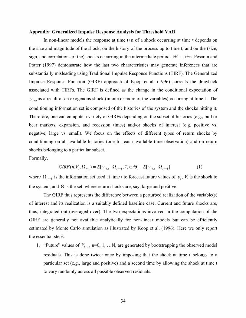
Appendix: Generalized Impulse Response Analysis for Threshold VAR

In non-linear models the response at time t+n of a shock occurring at time t depends on

the size and magnitude of the shock, on the history of the process up to time t, and on the (size,

sign, and correlations of the) shocks occurring in the intermediate periods t+1,…t+n. Pesaran and

Potter (1997) demonstrate how the last two characteristics may generate inferences that are

substantially misleading using Traditional Impulse Response Functions (TIRF). The Generalized

Impulse Response Function (GIRF) approach of Koop et al. (1996) corrects the drawback

associated with TIRFs. The GIRF is defined as the change in the conditional expectation of

nty + as a result of an exogenous shock (in one or more of the variables) occurring at time t. The

conditioning information set is composed of the histories of the system and the shocks hitting it.

Therefore, one can compute a variety of GIRFs depending on the subset of histories (e.g., bull or

bear markets, expansion, and recession times) and/or shocks of interest (e.g. positive vs.

negative, large vs. small). We focus on the effects of different types of return shocks by

conditioning on all available histories (one for each available time observation) and on return

shocks belonging to a particular subset.

Formally,

]|[],|[),,( 111 −−+−−+− Ω−Θ∈Ω=Ω tntttnttt yEVyEVnGIRF (1)

where 1−−Ωt is the information set used at time t to forecast future values of ty , Vt is the shock to

the system, and Θ is the set where return shocks are, say, large and positive.

The GIRF thus represents the difference between a perturbed realization of the variable(s)

of interest and its realization is a suitably defined baseline case. Current and future shocks are,

thus, integrated out (averaged over). The two expectations involved in the computation of the

GIRF are generally not available analytically for non-linear models but can be efficiently

estimated by Monte Carlo simulation as illustrated by Koop et al. (1996). Here we only report

the essential steps.

1. “Future” values of ntV + , n=0, 1, …N, are generated by bootstrapping the observed model

residuals. This is done twice: once by imposing that the shock at time t belongs to a

particular set (e.g., large and positive) and a second time by allowing the shock at time t

to vary randomly across all possible observed residuals.

35

2. Using the two simulated set of disturbances we then generate two sets of “future” values

of nty + , n=0, 1, …N starting from a given history, 11 −− =Ω tt ϖ , and iterating by following

the rules of the time series model in equation (1).

3. We repeat 1 and 2 for each available history (i.e., time series observation).

4. We repeat 1, 2, and 3 R times.

By the law of large numbers, the averages across simulations converge to the

expectations in (1). In our applications we set R = 5000 and simulate the systems for N=20 steps

ahead. We then standardized the responses so that they have a value of 1 at time t+1 and

cumulate them over 20 periods. We are especially interested in the reaction of turnover to

different return shocks and we, thus, conduct several experiments. Namely, we compute and

compare the GIRF of turnover for:

(a) positive return shocks and negative return shocks,

(b) large (bigger than 1 or 2 standard deviations) positive return shocks and large negative

return shocks, and

(c) large (between 1 or 2 standard deviations) positive return shocks and small (between 0 or

1 standard deviations) positive return shocks.

The difference between (b) and (c) is that in (b) we compare large positive to large negative and

in (c) we compare large to small shocks of the same sign.

36

Figu

re 1

Im

puls

e R

espo

nse

Func

tions

from

Biv

aria

te V

AR

U

sing

wee

kly

retu

rns

and

detre

nded

turn

over

dat

a fr

om J

anua

ry 2

, 199

3 to

Jun

e 30

, 200

3 w

e es

timat

e bi

varia

te V

AR

s of

det

rend

ed

turn

over

and

retu

rns.

Turn

over

is to

tal t

rade

d va

lue

in a

giv

en w

eek

scal

ed b

y th

e w

eek’

s to

tal m

arke

t cap

italiz

atio

n. T

urno

ver i

s th

en

detre

nded

by

subt

ract

ing

a 20

-wee

k m

ovin

g av

erag

e. T

he fi

gure

repo

rts th

e G

ener

aliz

ed Im

puls

e R

espo

nse

Func

tion

(GIR

F) r

espo

nse

of tu

rnov

er to

a o

ne s

tand

ard

devi

atio

n sh

ock

to re

turn

s at

lags

one

, fiv

e, a

nd te

n w

eeks

. In

sign

ifica

nt b

ars

are

strip

ed a

nd s

igni

fican

t ba

rs a

re in

sol

id c

olor

s. H

igh-

inco

me

coun

tries

are

in a

lpha

betic

al o

rder

on

the

left

side

of t

he g

raph

and

dev

elop

ing

coun

tries

are

on

the

right

side

.

-0.7

-0.2

0.3

0.8

1.3

1.8

Australia

Austria

Belgium

Canada

Denmark

Finland

France

Germany

Greece

Hong Kong

Ireland

Israel

Italy

Japan

Luxembourg

N. Zealand

Netherlands

Norway

Portugal

Singapore

Spain

Sweden

Switzerland

Taiwan

U.K

U.S.A

Argentina

Brazil

Chile

China

Colombia

Czech Republic

Hungary

India

Indonesia

Malaysia

Mexico

Peru

Philippines

Poland

Russia

South Africa

South Korea

Thailand

Turkey

Venezuela

Response in Standard Deviations

Lag 1

Lag 5

Lag 1

0

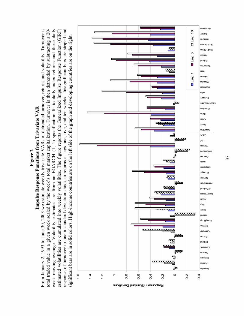
37

Figu

re 2

Im

puls

e R

espo

nse

Func

tions

from

Tri

vari

ate

VA

R

From

Jan

uary

2, 1

993

to J

une

30, 2

003

we

estim

ate

wee

kly

triva

riate

VA

Rs

of d

etre

nded

turn

over

, ret

urns

and

vol

atili

ty. T

urno

ver i

s to

tal t

rade

d va

lue

in a

giv

en w

eek

scal

ed b

y th

e w

eek’

s to

tal m

arke

t cap

italiz

atio

n. T

urno

ver

is th

en d

etre

nded

by

subt

ract

ing

a 20

-w

eek

mov

ing

aver

age.

Vol

atili

ty e

stim

ates

are

fro

m a

n EG

AR

CH

(1,

1)

spec

ifica

tion

fit t

o da

ily i

ndex

ret

urns

and

the

se d

aily

es

timat

ed v

olat

ilitie

s ar

e cu

mul

ated

into

wee

kly

vola

tiliti

es. T

he f

igur

e re

ports

the

Gen

eral

ized

Im

puls

e R

espo

nse

Func

tion

(GIR

F)

resp

onse

of t

urno

ver t

o on

e a

stan

dard

dev

iatio

n sh

ock

to re

turn

s at

lags

one

, fiv

e, a

nd te

n w

eeks

. In

sign

ifica

nt b

ars

are

strip

ed a

nd

sign

ifica

nt b

ars a

re in

solid

col

ors.

Hig

h-in

com

e co

untri

es a

re o

n th

e le

ft si

de o

f the

gra

ph a

nd d

evel

opin

g co

untri

es a

re o

n th

e rig

ht.

-0.4

-0.20

0.2

0.4

0.6

0.81

1.2

1.4

1.6

Australia

Austria

Belgium

Canada

Denmark

Finland

France

Germany

Greece

Hong Kong

Ireland

Israel

Italy

Japan

Luxembourg

N. Zealand

Netherlands

Norway

Portugal

Singapore

Spain

Sweden

Switzerland

Taiwan

U.K

U.S.A

Argentina

Brazil

Chile

China

Colombia

Czech Republic

Hungary

India

Indonesia

Malaysia

Mexico

Peru

Philippines

Poland

Russia

South Africa

South Korea

Thailand

Turkey

Venezuela

Response in Standard Deviations

La

g 1

Lag

5L

ag 1

0

38

Fi

gure

3

Impu

lse

Res

pons

e Fu

nctio

ns fr

om T

riva

riat

e V

AR

with

Squ

ared

Res

idua

l Vol

atili

ty a

nd N

on-D

etre

nded

Tur

nove

r U

sing

wee

kly

retu

rn a

nd d

etre

nded

turn

over

dat

a fr

om J

anua

ry 2

, 199

3 to

Jun

e 30

, 200

3 w

e es

timat

e th

e fo

llow

ing

triva

riate

VA

Rs

a)

Det

rend

ed T

urno

ver,

Ret

urns

and

EG

AR

CH

Vol

atili

ty, b

) D

etre

nded

Tur

nove

r, R

etur

ns a

nd S

quar

ed R

esid

uals

Vol

atili

ty, c

) R

aw

Turn

over

, Ret

urns

and

EG

AR

CH

Vol

atili

ty. R

aw T

urno

ver

is to

tal t

rade

d va

lue

in a

giv

en w

eek

scal

ed b

y th

e w

eek’

s to

tal m

arke

t ca

pita

lizat

ion.

Det

rend

ed T

urno

ver

is t

hen

com

pute

d by

sub

tract

ing

a 20

-wee

k m

ovin

g av

erag

e fr

om R

aw T

urno

ver.

EGA

RC

H

Vol

atili

ty e

stim

ates

are

fro

m a

n EG

AR

CH

(1,

1)

spec

ifica

tion

fit t

o da

ily i

ndex

ret

urns

and

the

se d

aily

est

imat

ed v

olat

ilitie

s ar

e cu

mul

ated

into

wee

kly

vola

tiliti

es. S

quar

ed R

esid

uals

Vol

atili

ty is

com

pute

d by

squa

ring

the

resi

dual

s of a

n A

R (1

) mod

el fi

tted

to th

e re

turn

s se

ries.

The

figur

e re

ports

the

GIR

F re

spon

se o

f tu

rnov

er t

o a

one

stan

dard

dev

iatio

n sh

ock

to r

etur

ns a

t la

g 10

wee

ks.

Insi

gnifi

cant

bar

s ar

e st

riped

and

sig

nific

ant

bars

are

in

solid

col

ors.

Hig

h-in

com

e co

untri

es a

re o

n th

e le

ft si

de o

f th

e gr

aph

and

deve

lopi

ng c

ount

ries a

re o

n th

e rig

ht.

-1.4

-0.9

-0.4

0.1

0.6

1.1

1.6

2.1

2.6

Australia

Austria

Belgium

Canada

Denmark

Finland

France

Germany

Greece

Hong Kong

Ireland

Israel

Italy

Japan

Luxembourg

N. Zealand

Netherlands

Norway

Portugal

Singapore

Spain

Sweden

Switzerland

Taiwan

U.K

U.S.A

Argentina

Brazil

Chile

China

Colombia

Czech Republic

Hungary

India

Indonesia

Malaysia

Mexico

Peru

Philippines

Poland

Russia

South Africa

South Korea

Thailand

Turkey

Venezuela

Lag 10: Response in Standard Deviations

De

trended T

urn

over,

Retu

rns a

nd E

GA

RC

HV

ola

tilit

y

De

trended T

urn

over,

Retu

rns a

nd S

quare

dR

esid

uals

Vo

latilit

y

Ra

w T

urn

over,

Retu

rns a

nd E

GA

RC

H V

ola

tilit

y

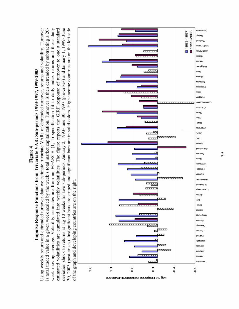
39

Figu

re 4

Im

puls

e R

espo

nse

Func

tions

from

Tri

vari

ate

VA

R: S

ub-p

erio

ds 1

993-

1997

, 199

9-20

03

Usi

ng w

eekl

y re

turn

and

det

rend

ed tu

rnov

er d

ata

we

estim

ate

triva

riate

VA

Rs

of d

etre

nded

turn

over

, ret

urns

and

vol

atili

ty. T

urno

ver

is to

tal t

rade

d va

lue

in a

giv

en w

eek

scal

ed b

y th

e w

eek’

s to

tal m

arke

t cap

italiz

atio

n. T

urno

ver i

s th

en d

etre

nded

by

subt

ract

ing

a 20

-w

eek

mov

ing

aver

age.

Vol

atili

ty e

stim

ates

are

fro

m a

n EG

AR

CH

(1,

1)

spec

ifica

tion

fit t

o da

ily i

ndex

ret

urns

and

the

se d

aily

es

timat

ed v

olat

ilitie

s ar

e cu

mul

ated

int

o w

eekl

y vo

latil

ities

. Th

e fig

ure

repo

rts t

he G

IRF

resp

onse

of

turn

over

to

one

a st

anda

rd

devi

atio

n sh

ock

to re

turn

s at

lag

10 w

eeks

for t

wo

sub-

perio

ds: J

anua

ry 2

, 199

3-Ju

ne 3

0, 1

997

(pre

-cris

es) a

nd J

anua

ry 1

, 199

9- J

une

30, 2

003

(pos

t cris

es).

Insi

gnifi

cant

bar

s ar

e st

riped

and

sig

nific

ant b

ars

are

in s

olid

col

ors.

Hig

h-in

com

e co

untri

es a

re o

n th

e le

ft si

de

of th

e gr

aph

and

deve

lopi

ng c

ount

ries a

re o

n th

e rig

ht.

-0.9

-0.4

0.1

0.6

1.1

1.6

Australia

Austria

Belgium

Canada

Denmark

Finland

France

Germany

Greece

Hong Kong

Ireland

Israel

Italy

Japan

Luxembourg

N. Zealand

Netherlands

Norway

Portugal

Singapore

Spain

Sweden

Switzerland

Taiwan

U.K

U.S.A

Argentina

Brazil

Chile

China

Colombia

Czech Republic

Hungary

India

Indonesia

Malaysia

Mexico

Peru

Philippines

Poland

Russia

South Africa

South Korea

Thailand

Turkey

Venezuela

Lag 10: Response in Standard Deviations

1993

-1997

1999

-2003

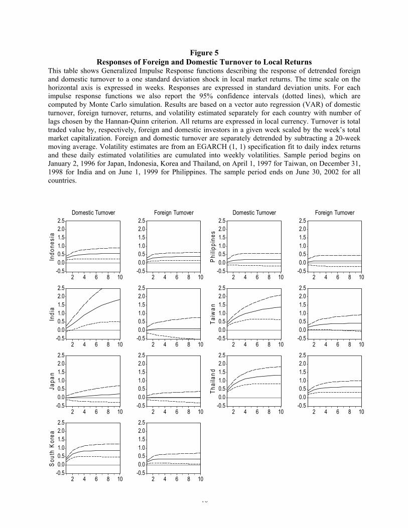
40

Figure 5 Responses of Foreign and Domestic Turnover to Local Returns

This table shows Generalized Impulse Response functions describing the response of detrended foreign and domestic turnover to a one standard deviation shock in local market returns. The time scale on the horizontal axis is expressed in weeks. Responses are expressed in standard deviation units. For each impulse response functions we also report the 95% confidence intervals (dotted lines), which are computed by Monte Carlo simulation. Results are based on a vector auto regression (VAR) of domestic turnover, foreign turnover, returns, and volatility estimated separately for each country with number of lags chosen by the Hannan-Quinn criterion. All returns are expressed in local currency. Turnover is total traded value by, respectively, foreign and domestic investors in a given week scaled by the week’s total market capitalization. Foreign and domestic turnover are separately detrended by subtracting a 20-week moving average. Volatility estimates are from an EGARCH (1, 1) specification fit to daily index returns and these daily estimated volatilities are cumulated into weekly volatilities. Sample period begins on January 2, 1996 for Japan, Indonesia, Korea and Thailand, on April 1, 1997 for Taiwan, on December 31, 1998 for India and on June 1, 1999 for Philippines. The sample period ends on June 30, 2002 for all countries.

-0.50.00.51.01.52.02.5

2 4 6 8 10

Domestic Turnover

Indo

nesi

a

-0.50.00.51.01.52.02.5

2 4 6 8 10

Foreign Turnover

-0.50.00.51.01.52.02.5

2 4 6 8 10

Domestic TurnoverP

hilip

pine

s

-0.50.00.51.01.52.02.5

2 4 6 8 10

Foreign Turnover

-0.50.00.51.01.52.02.5

2 4 6 8 10

Indi

a

-0.50.00.51.01.52.02.5

2 4 6 8 10-0.50.00.51.01.52.02.5

2 4 6 8 10

Taiw

an

-0.50.00.51.01.52.02.5

2 4 6 8 10

-0.50.00.51.01.52.02.5

2 4 6 8 10

Japa

n

-0.50.00.51.01.52.02.5

2 4 6 8 10-0.50.00.51.01.52.02.5

2 4 6 8 10

Thai

land

-0.50.00.51.01.52.02.5

2 4 6 8 10

-0.50.00.51.01.52.02.5

2 4 6 8 10

Sou

th K

orea

-0.50.00.51.01.52.02.5

2 4 6 8 10

41

Figure 6 Responses of Institutional, Individual and Foreign Turnover to Local Returns

This table shows Generalized Impulse Response functions describing the response of detrended foreign, domestic institutional, and domestic individual turnover to a one standard deviation shock in local market returns. The time scale on the horizontal axis is expressed in weeks. Responses are expressed in standard deviation units. For each impulse response functions we also report the 95% confidence intervals (dotted lines), which are computed by Monte Carlo simulation. Results are based on a VAR of domestic institutional turnover, domestic individual turnover, foreign turnover, returns, and volatility estimated separately for each country with number of lags chosen by the Hannan-Quinn criterion. All returns are expressed in local currency. Turnover is total traded value by, respectively, foreign, domestic institutional, and domestic individual investors in a given week scaled by the week’s total market capitalization. Foreign, domestic institutional, and domestic individual turnover are separately detrended by subtracting a 20-week moving average. Volatility estimates are from an EGARCH (1, 1) specification fit to daily index returns and these daily estimated volatilities are cumulated into weekly volatilities. Sample period begins on January 2, 1996 for Japan, Korea and Thailand, on April 1, 1997 for Taiwan, on December 31, 1198 for India and on June 1, 1999 for Philippines. The sample period ends on June 30, 2002 for all countries.

-0.50.00.51.01.52.02.5

2 4 6 8 10

Institutional Turnover

Japa

n

-0.50.00.51.01.52.02.5

2 4 6 8 10

Sout

h K

orea

-0.50.00.51.01.52.02.5

2 4 6 8 10

Taiw

an

-0.50.00.51.01.52.02.5

2 4 6 8 10

Thai

land

-0.50.00.51.01.52.02.5

2 4 6 8 10

Individual Turnover

-0.50.00.51.01.52.02.5

2 4 6 8 10

-0.50.00.51.01.52.02.5

2 4 6 8 10

-0.50.00.51.01.52.02.5

2 4 6 8 10

-0.50.00.51.01.52.02.5

2 4 6 8 10

Foreign Turnover

-0.50.00.51.01.52.02.5

2 4 6 8 10

-0.50.00.51.01.52.02.5

2 4 6 8 10

-0.50.00.51.01.52.02.5

2 4 6 8 10

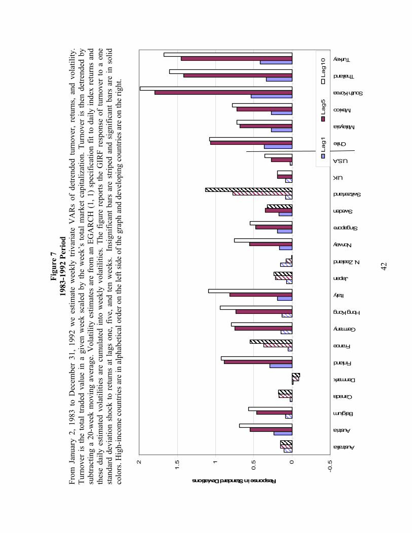
42

Figu

re 7

19

83-1

992

Peri

od

From

Jan

uary

2,

1983

to

Dec

embe

r 31

, 19

92 w

e es

timat

e w

eekl

y tri

varia

te V

AR

s of

det

rend

ed t

urno

ver,

retu

rns,

and

vola

tility

. Tu

rnov

er is

the

tota

l tra

ded

valu

e in

a g

iven

wee

k sc

aled

by

the

wee

k’s

tota

l mar

ket c

apita

lizat

ion.

Tur

nove

r is

then

det

rend

ed b

y su

btra

ctin

g a

20-w

eek

mov

ing

aver

age.

Vol

atili

ty e

stim

ates

are

fro

m a

n EG

AR

CH

(1,

1)

spec

ifica

tion

fit to

dai

ly in

dex

retu

rns

and

thes

e da

ily e

stim

ated

vol

atili

ties

are

cum

ulat

ed in

to w

eekl

y vo

latil

ities

. The

fig

ure

repo

rts th

e G

IRF

resp

onse

of

turn

over

to a

one

st

anda

rd d

evia

tion

shoc

k to

ret

urns

at l

ags

one,

fiv

e, a

nd te

n w

eeks

. In

sign

ifica

nt b

ars

are

strip

ed a

nd s

igni

fican

t bar

s ar

e in

sol

id

colo

rs. H

igh-

inco

me

coun

tries

are

in a

lpha

betic

al o

rder

on

the

left

side

of t

he g

raph

and

dev

elop

ing

coun

tries

are

on

the

right

.

-0.50

0.51

1.52

Australia

Austria

Belgium

Canada

Denmark

Finland

France

Germany

Hong Kong

Italy

Japan

N. Zealand

Norway

Singapore

Sweden

Switzerland

U.K

U.S.A

Chile

Malaysia

Mexico

South Korea

Thailand

Turkey

Response in Standard Deviations

Lag1

Lag5

Lag10

43

Tab

le I

Sum

mar

y St

atis

tics

Wee

kly

Dat

aStre

am d

ata

from

46

mar

kets

is u

sed

with

the

begi

nnin

g of

cov

erag

e m

arke

d in

the

first

col

umn

and

endi

ng o

n Ju

ne 3

0, 2

003

for a

ll co

untri

es. F

or e

ach

coun

try, w

e re

port

the

mea

n (µ

), st

anda

rd d

evia

tion

(σ),

and

lag

1 au

toco

rrel

atio

n co

effic

ient

for

wee

kly

valu

e-w

eigh

ted

retu

rns,

EGA

RC

H v

olat

ility

, tur

nove

r, an

d de

trend

ed tu

rnov

er. U

nits

are

per

cent

per

wee

k. W

e al

so re

port

sim

ple

corr

elat

ion

coef

ficie

nts

in e

ach

mar

ket b

etw

een

lagg

ed tu

rnov

er a

nd re

turn

s, th

e co

ntem

pora

neou

s co

rrel

atio

n be

twee

n tu

rnov

er a

nd re

turn

s, th

e co

rrel

atio

n be

twee

n tu

rnov

er in

th

e ne

xt tw

o pe

riods

and

retu

rns

as w

ell a

s th

e co

ntem

pora

neou

s co

rrel

atio

n be

twee

n re

turn

s an

d EG

AR

CH

vol

atili

ty a

nd v

olat

ility

and

turn

over

. EG

AR

CH

vol

atili

ty e

stim

ates

are

fro

m a

n EG

AR

CH

(1,

1)

spec

ifica

tion

fit t

o da

ily i

ndex

ret

urns

and

the

se d

aily

est

imat

ed v

olat

ilitie

s ar

e cu

mul

ated

into

wee

kly

vola

tiliti

es. T

urno

ver i

s de

trend

ed b

y fir

st ta

king

its

natu

ral l

og a

nd th

en s

ubtra

ctin

g its

200

-day

mov

ing

aver

age.

Pan

el A

re

ports

resu

lts fo

r hig

h in

com

e m

arke

ts, w

here

as P

anel

B re

ports

resu

lts fo

r dev

elop

ing

mar

kets

. The

sep

arat

ion

com

es fr

om u

sing

199

8 W

orld

B

ank

clas

sific

atio

ns to

sep

arat

e ou

r sam

ple

into

hig

h in

com

e (d

evel

oped

) mar

kets

and

upp

er m

iddl

e in

com

e, m

iddl

e in

com

e, a

nd lo

wer

mid

dle

inco

me

mar

kets

whi

ch w

e re

fer t

o as

dev

elop

ing.

Pa

nel A

: Hig

h in

com

e M

arke

ts R

etur

n V

olat

ility

T

urno

ver

Det

. Log

T

urno

ver

Lea

d-L

ag C

orre

latio

ns

Cou

ntry

Fr

om

µ(%

) σ(

%)

AC

(1)

µ(%

)A

C(1

)µ(

%)

AC

(1)

µ A

C(1

) T

t-1,

Rt

Tt,

Rt

Tt+

1, R

tR

t, V

t T

t, V

t

Aus

tralia

19

93

0.20

2.

02

-0.1

4*

1.78

0.

75*

1.03

0.

50*

0.01

0.

22*

0.02

0.

01

-0.1

0*

-0.0

8 0.

15*

Aus

tria

1993

0.

12

1.89

0.

00

1.58

0.

86*

0.98

0.

73*

0.00

0.

48*

0.08

* 0.

07

0.04

-0

.15*

0.

12*

Bel

gium

19

93

0.17

2.

52

-0.0

7 1.

87

0.94

* 0.

43

0.51

* 0.

01

0.35

* 0.

05

0.01

-0

.05

-0.0

5 0.

07

Can

ada

1993

0.

22

2.16

-0

.05

1.86

0.

91*

1.07

0.

67*

0.01

0.

37*

0.03

-0

.03

-0.0

4 -0

.12*

0.

20*

Den

mar

k 19

93

0.23

2.

39

0.05

2.

08

0.72

* 0.

74

0.50

* 0.

01

0.28

* -0

.03

0.06

0.

06

-0.0

6 0.

14*

Finl

and

1993

0.

41

4.99

-0

.07

4.44

0.

93*

1.02

0.

80*

0.04

0.

43*

0.02

0.

03

-0.0

3 -0

.08*

0.

06*

Fran

ce

1993

0.

18

2.87

-0

.10*

2.

60

0.94

* 1.

30

0.72

* 0.

02

0.34

* 0.

00

-0.0

3 -0

.10*

-0

.08*

0.

16*

Ger

man

y 19

93

0.14

2.

92

-0.0

6 2.

49

0.90

* 2.

84

0.74

* -0

.08

0.74

* 0.

03

0.04

0.

02

-0.1

0*

0.03

G

reec

e 19

93

0.26

4.

17

-0.0

1 3.

37

0.75

* 0.

71

0.78

* 0.

02

0.49

* 0.

03

0.14

* 0.

21*

-0.0

4 0.

18*

Hon

g K

ong

1993

0.

15

4.26

-0

.08

3.43

0.

81*

0.86

0.

57*

0.00

0.

44*

0.07

0.

11*

0.07

-0

.03

0.17

* Ir

elan

d 20

01

-0.1

4 3.

00

0.12

2.

76

0.74

* 0.

81

0.80

* 0.

13

0.72

* -0

.04

0.00

-0

.15

-0.2

7*

0.21

* Is

rael

19

93

0.19

3.

23

-0.0

3 3.

04

0.59

* 0.

34

0.84

* 0.

15

0.69

* -0

.01

0.04

0.

00

-0.1

6*

0.19

* Ita

ly

1993

0.

20

3.27

0.

01

2.95

0.

84*

1.52

0.

81*

0.04

0.

55*

0.06

0.

13*

0.10

* -0

.08

0.11

* Ja

pan

1993

-0

.04

2.73

-0

.05

2.57

0.

82*

0.80

0.

54*

0.01

0.

51*

0.04

0.

12*

0.06

-0

.04

0.19

* Lu

xem

bour

g 19

99

-0.1

0 3.

15

0.23

* 2.

66

0.65

* 0.

05

0.72

* -0

.07

0.47

* 0.

07

0.20

* 0.

04

-0.1

8*

0.20

* N

. Zea

land

19

93

0.18

2.

21

-0.0

6 1.

90

0.39

* 0.

64

0.40

* 0.

01

0.37

* -0

.03

0.06

0.

03

0.07

0.

10*

Net

herla

nds

1993

0.

20

2.69

-0

.05

2.40

0.

95*

2.10

0.

80*

0.01

0.

45*

-0.0

2 -0

.07

-0.0

9*

-0.0

9*

0.15

* N

orw

ay

1993

0.

19

2.70

0.

01

2.36

0.

81*

1.29

0.

39*

0.01

0.

21*

-0.0

2 0.

08

0.02

-0

.19*

0.

15*

44

Portu

gal

1993

0.

19

2.40

0.

09*

1.92

0.

78*

0.79

0.

61*

0.08

0.

56*

0.17

* 0.

21*

0.16

* -0

.07

-0.0

2 Si

ngap

ore

1993

0.

04

3.03

-0

.01

2.56

0.

82*

0.66

0.

77*

0.02

0.

49*

0.07

0.

16*

0.08

0.

03

0.24

* Sp

ain

1993

0.

27

2.85

-0

.05

2.61

0.

91*

1.42

0.

75*

0.02

0.

35*

0.02

0.

04

0.02

-0

.12*

0.

16*

Swed

en

1993

0.

25

3.50

-0

.09*

3.

08

0.89

* 1.

52

0.76

* 0.

02

0.43

* 0.

01

-0.0

2 -0

.02*

-0

.09*

0.

21*

Switz

erla

nd

1993

0.

19

2.61

-0

.08

2.17

0.

90*

1.28

0.

58*

0.01

0.

37*

-0.0

1 -0

.07

-0.0

9 -0

.15*

0.

22*

Taiw

an

1993

0.

16

4.09

0.

06

3.90

0.

76*

3.42

0.

75*

-0.0

1 0.

65*

0.11

* 0.

35*

0.30

* -0

.06

0.23

* U

.K

1993

0.

14

2.26

-0

.09*

2.

03

0.94

* 1.

48

0.81

* 0.

02

0.37

* 0.

02

-0.0

3 -0

.08*

-0

.05

0.17

* U

.S.A

. 19

93

0.19

2.

47

-0.1

4*

2.24

0.

90*

2.26

0.

80*

0.01

0.

26*

0.07

0.

05

-0.0

6 -0

.06

0.17

* M

ean,

Hig

h in

com

e 0.

16

2.94

-0

.03

2.56

0.

82

1.21

0.

68

0.02

0.

45

0.03

0.

06

0.01

-0

.09

0.15

Pa

nel B

: Dev

elop

ing

mar

kets

Ret

urn

Vol

atili

ty

Tur

nove

r D

et. L

og

Tur

nove

r L

ead-

Lag

Cor

rela

tions

C

ount

ry

From

µ(

%)

σ(%

) A

C(1

)µ(

%)

AC

(1)

µ(%

)A

C(1

) µ

AC

(1)

Tt-

1, R

tT

t, R

tT

t+1,

Rt

Rt,

Vt

Tt,

Vt

Arg

entin

a 19

93

0.21

4.

67

0.00

3.

89

0.78

* 0.

29

0.73

* -0

.01

0.50

* 0.

00

0.25

* 0.

01

-0.0

2 0.

26*

Bra

zil

1999

0.

43

3.68

-0

.06

3.06

0.

68*

0.73

0.

37*

-0.0

3 0.

32*

-0.0

7 0.

10

-0.0

3 0.

14*

0.14

* C

hile

19

93

0.21

2.

57

0.10

* 1.

81

0.82

* 0.

18

0.51

* 0.

01

0.40

* 0.

08

0.22

* 0.

10*

-0.0

1 0.

16*

Chi

na

1993

0.

13

5.47

-0

.05

4.01

0.

83*

3.43

0.

43*

-0.0

1 0.

65*

0.11

* 0.

33*

0.25

* 0.

02

0.04

* C

olom

bia

1993

0.

16

2.70

0.

18*

1.74

0.

34*

0.11

0.

33*

0.01

0.

24*

0.04

0.

17*

0.20

* 0.

13*

0.09

* C

zech

Rep

. 19

93

0.10

3.

82

0.07

2.

72

0.92

* 0.

50

0.82

* 0.

10

0.67

* -0

.08

-0.0

6 -0

.05

0.14

* 0.

30*

Hun

gary

19

93

0.39

4.

35

0.01

3.

49

0.43

* 2.

78

0.41

* 0.

07

0.49

* 0.

00

0.17

* 0.

08

0.00

0.

05*

Indi

a 19

95

0.06

4.

10

-0.0

2 3.

28

0.69

* 1.

31

0.94

* 0.

07

0.72

* 0.

04

0.15

* 0.

14*

-0.1

8*

-0.0

6 In

done

sia

1993

0.

14

4.74

-0

.08

3.69

0.

87*

0.48

0.

62*

0.04

0.

40*

0.03

0.

23*

0.05

0.

02

0.16

* M

alay

sia

1993

0.

08

4.23

-0

.04

3.05

0.

69*

0.47

0.

65*

-0.0

1 0.

51*

0.05

0.

23*

0.13

* 0.

09*

0.11

* M

exic

o 19

93

0.26

3.

46

0.03

2.

95

0.84

* 0.

83

0.54

* -0

.01

0.41

* -0

.02

0.22

* 0.

11*

-0.1

1*

0.09

* Pe

ru

1994

0.

23

2.98

0.

02

2.35

0.

90*

0.46

0.

08

-0.0

5 0.

55*

-0.0

2 0.

04

0.02

0.

04

0.06

Ph

ilipp

ines

19

93

0.08

3.

79

0.02

2.

87

0.79

* 0.

34

0.54

* 0.

00

0.41

* 0.

18*

0.25

* 0.

15*

-0.0

5 0.

26*

Pola

nd

1994

-0

.04

5.36

0.

04

4.13

0.

75*

0.69

0.

76*

-0.0

3 0.

55*

-0.0

5 0.

27*

0.21

* -0

.06

0.16

* R

ussi

a 19

95

0.48

6.

74

0.06

5.

56

0.51

* 0.

16

0.71

* 0.

01

0.55

* 0.

05

0.26

* 0.

18*

-0.0

9 0.

02

Sout

h A

fric

a 19

93

0.28

3.

16

-0.0

3 2.

35

0.68

* 0.

60

0.77

* 0.

03

0.48

* -0

.06

0.04

-0

.05*

-0

.04

0.13

* So

uth

Kor

ea

1993

0.

12

5.07

-0

.06

4.53

0.

91*

2.61

0.

82*

0.02

0.

61*

0.07

0.

28*

0.25

* 0.

02

0.29

* Th

aila

nd

1993

0.

00

5.15

0.

02

4.12

0.

86*

0.82

0.

67*

0.00

0.

57*

0.06

0.

36*

0.25

* 0.

05

0.25

* Tu

rkey

19

93

1.16

7.

46

0.06

6.

89

0.66

* 2.

27

0.65

* 0.

02

0.51

* 0.

08

0.34

* 0.

23*

-0.0

5 0.

25*

Ven

ezue

la

1993

0.

42

5.56

0.

07

4.53

0.

24*

0.42

0.

45*

-0.0

6 0.

45*

0.17

* 0.

27*

0.22

* 0.

12*

0.18

* M

ean,

Dev

elop

ing

0.24

4.

45

-0.0

2 3.

55

0.71

0.

97

0.59

0.

01

0.50

0.

03

0.21

0.

12

0.01

0.

15

Mea

n, A

ll 0.

20

3.69

0.

00

3.06

0.

76

1.09

0.

64

0.01

0.

47

0.03

0.

14

0.07

-0

.04

0.15

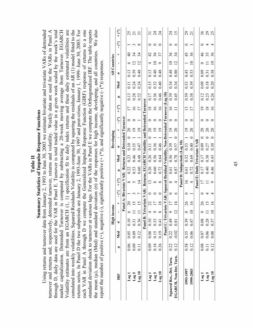
45

Tab

le II

Su

mm

ary

Stat

istic

s of I

mpu

lse

Res

pons

e Fu

nctio

ns

Usi

ng re

turn

s and

turn

over

dat

a fr

om Ja

nuar

y 2,

199

3 to

June

30,

200

3 w

e es

timat

e bi

varia

te a

nd tr

ivar

iate

VA

Rs

of d

etre

nded

tu

rnov

er a

nd r

etur

ns a

nd, r

espe

ctiv

ely,

det

rend

ed tu

rnov

er, r

etur

ns a

nd v

olat

ility

. W

eekl

y da

ta a

re u

sed

for

the

VA

Rs

in P

anel

A

thro

ugh

D, d

aily

dat

a ar

e us

ed f

or th

e V

AR

in P

anel

E. T

urno

ver

is to

tal t

rade

d va

lue

in a

giv

en w

eek

scal

ed b

y th

e w

eek’

s to

tal

mar

ket

capi

taliz

atio

n. D

etre

nded

Tur

nove

r is

com

pute

d by

sub

tract

ing

a 20

-wee

k m

ovin

g av

erag

e fr

om T

urno

ver.

EGA

RC

H

Vol

atili

ty e

stim

ates

are

fro

m a

n EG

AR

CH

(1,

1)

spec

ifica

tion

fit t

o da

ily i

ndex

ret

urns

and

the

se d

aily

est

imat

ed v

olat

ilitie

s ar

e cu

mul

ated

into

wee

kly

vola

tiliti

es. S

quar

ed R

esid

uals

Vol

atili

ty is

com

pute

d by

squa

ring

the

resi

dual

s of a

n A

R (1

) mod

el fi

tted

to th

e re

turn

s se

ries.

In P

anel

D th

e tw

o su

bper

iods

are

Jan

uary

2, 1

993-

June

30,

199

7 an

d po

st-c

rises

, Jan

uary

1, 1

999-

Jun

e 30

, 200

3. F

or

each

VA

R i

n Pa

nel

A t

hrou

gh D

we

com

pute

the

Gen

eral

ized

Im

puls

e R

espo

nse

Func

tion

(GIR

F) r

espo

nse

of r

etur

ns t

o a

one

stan

dard

dev

iatio

n sh

ock

to tu

rnov

er a

t var

ious

lags

. For

the

VA

Rs

in P

anel

E w

e co

mpu

te th

e O

rthog

onal

ized

IRF.

The

tabl

e re

ports

th

e m

ean

(µ),

med

ian

(Med

) an

d st

anda

rd d

evia

tion

(σ)

of th

e re

spon

ses

for

high

inco

me,

dev

elop

ing,

and

all

coun

tries

. W

e al

so

repo

rt th

e nu

mbe

r of p

ositi

ve (+

), ne

gativ

e (-

), si

gnifi

cant

ly p

ositi

ve (+

(*))

, and

sign

ifica

ntly

neg

ativ

e (-

(*))

resp

onse

s.

Hig

h in

com

e D

evel

opin

g A

ll C

ount

ries

IR

F µ

Med

σ

- +

- (*)

+

(*)

µ M

ed

σ -

+ - (

*)

+ (*

) µ

Med

σ

- +

- (*)

+

(*)

Pane

l A: B

ivar

iate

VA

R:

Ret

urns

and

Det

rend

ed T

urno

ver

Lag

1

0.06

0.

05

0.10

6

20

1 8

0.22

0.

23

0.10

0

20

0 17

0.

13

0.11

0.

13

6 40

1

25

Lag

5

0.09

0.

09

0.31

11

15

3

5 0.

53

0.46

0.

35

1 19

0

16

0.28

0.

24

0.39

12

34

3

21

Lag

10

0.11

0.

12

0.36

11

15

7

14

0.60

0.

48

0.47

1

19

1 17

0.

32

0.24

0.

48

12

34

8 31

Pa

nel B

: Tri

vari

ate

VA

R:

Ret

urns

, EG

AR

CH

Vol

atili

ty a

nd D

etre

nded

Tur

nove

r L

ag 1

0.

09

0.08

0.

10

4 22

0

13

0.26

0.

26

0.11

0

20

0 18

0.

17

0.15

0.

13

4 42

0

31

Lag

5

0.18

0.

15

0.33

9

17

0 8

0.60

0.

56

0.36

1

19

0 16

0.

36

0.32

0.

40

10

36

0 24

L

ag 1

0 0.

26

0.19

0.

41

8 18

0

8 0.

72

0.64

0.

46

1 19

0

16

0.46

0.

40

0.48

9

37

0 24

Pa

nel C

: Tri

vari

ate

VA

R: S

quar

ed R

esid

ual V

olat

ility

, Non

-Det

rend

ed T

urno

ver

(Lag

10)

Sq

uare

d R

es.,

Det

. Tur

n.

0.22

0.

22

0.49

9

17

0 8

0.61

0.

56

0.39

1

19

0 16

0.

39

0.34

0.

48

10

36

0 24

E

GA

RC

H, N

on-D

et. T

urn.

0.

12

-0.0

2 0.

81

12

14

6 4

0.87

0.

78

0.57

0

20

0 11

0.

45

0.34

0.

80

12

34

6 15

Pa

nel D

: Sub

peri

ods (

Lag

10)

19

93-1

997

0.58

0.

55

0.39

0

26

0 16

0.

61

0.52

0.

53

1 19

0

13

0.59

0.

53

0.45

1

45

0 29

19

99-2

003

0.12

0.

06

0.47

10

16

1

4 0.

72

0.69

0.

40

0 20

0

17

0.38

0.

39

0.53

10

36

1

21

Pane

l E: D

aily

Tri

vari

ate

VA

R

Lag

1

0.08

0.

07

0.08

0

26

0 17

0.

17

0.17

0.

09

0 20

0

19

0.12

0.

09

0.09

0

46

0 36

L

ag 5

0.

11

0.06

0.

28

11

15

4 11

0.

40

0.38

0.

27

0 20

0

18

0.23

0.

18

0.31

11

35

4

29

Lag

10

0.12

0.

08

0.37

10

16

4

9 0.

46

0.43

0.

30

0 20

0

16

0.26

0.

20

0.38

10

36

4

25

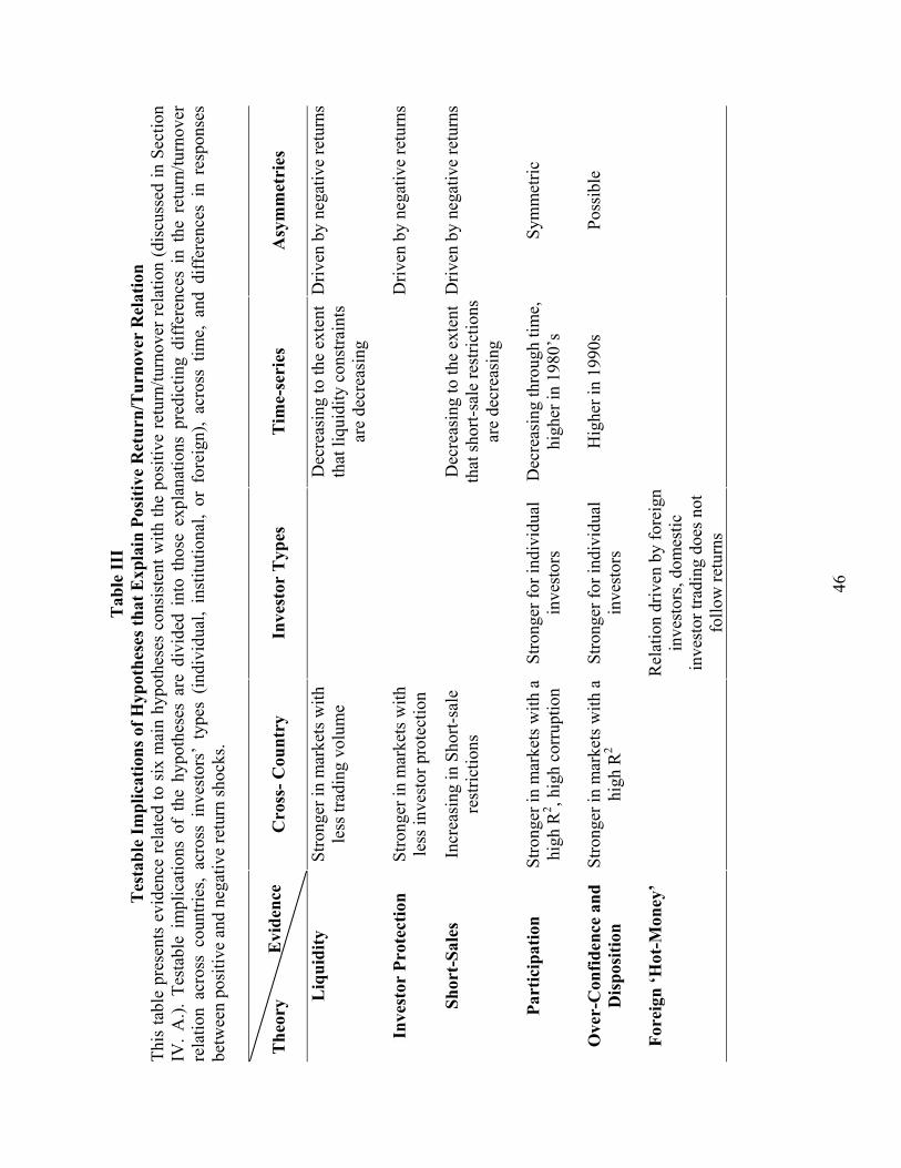
46

Tab

le II

I T

esta

ble

Impl

icat

ions

of H

ypot

hese

s tha

t Exp

lain

Pos

itive

Ret

urn/

Tur

nove

r R

elat

ion

This

tabl

e pr

esen

ts e

vide

nce

rela

ted

to s

ix m

ain

hypo

thes

es c

onsi

sten

t with

the

posi

tive

retu

rn/tu

rnov

er re

latio

n (d

iscu

ssed

in S

ectio

n IV

. A

.). T

esta

ble

impl

icat

ions

of

the

hypo

thes

es a

re d

ivid

ed i

nto

thos

e ex

plan

atio

ns p

redi

ctin

g di

ffer

ence

s in

the

ret

urn/

turn

over

re

latio

n ac

ross

cou

ntrie

s, ac

ross

inv

esto

rs’

type

s (in

divi

dual

, in

stitu

tiona

l, or

for

eign

), ac

ross

tim

e, a

nd d

iffer

ence

s in

res

pons

es

betw

een

posi

tive

and

nega

tive

retu

rn sh

ocks

.

Cro

ss- C

ount

ry

Inve

stor

Typ

es

Tim

e-se

ries

A

sym

met

ries

Liq

uidi

ty

Stro

nger

in m

arke

ts w

ith

less

trad

ing

volu

me

D

ecre

asin

g to

the

exte

nt

that

liqu

idity

con

stra

ints

ar

e de

crea

sing

Driv

en b

y ne

gativ

e re

turn

s

Inve

stor

Pro

tect

ion

Stro

nger

in m

arke

ts w

ith

less

inve

stor

pro

tect

ion

Driv

en b

y ne

gativ

e re

turn

s

Shor

t-Sa

les

Incr

easi

ng in

Sho

rt-sa

le

rest

rictio

ns

D

ecre

asin

g to

the

exte

nt

that

shor

t-sal

e re

stric

tions

ar

e de

crea

sing

Driv

en b

y ne

gativ

e re

turn

s

Part

icip

atio

n

Stro

nger

in m

arke

ts w

ith a

hi

gh R

2 , hig

h co

rrup

tion

Stro

nger

for i

ndiv

idua

l in

vest

ors

Dec

reas

ing

thro

ugh

time,

hi

gher

in 1

980’

s Sy

mm

etric

Ove

r-C

onfid

ence

and

D

ispo

sitio

n

Stro

nger

in m

arke

ts w

ith a

hi

gh R

2 St

rong

er fo

r ind

ivid

ual

inve

stor

s H

ighe

r in

1990

s Po

ssib

le

Fore

ign

‘Hot

-Mon

ey’

R

elat

ion

driv

en b

y fo

reig

n in

vest

ors,

dom

estic

in

vest

or tr

adin

g do

es n

ot

follo

w re

turn

s

The

ory

Evi

denc

e

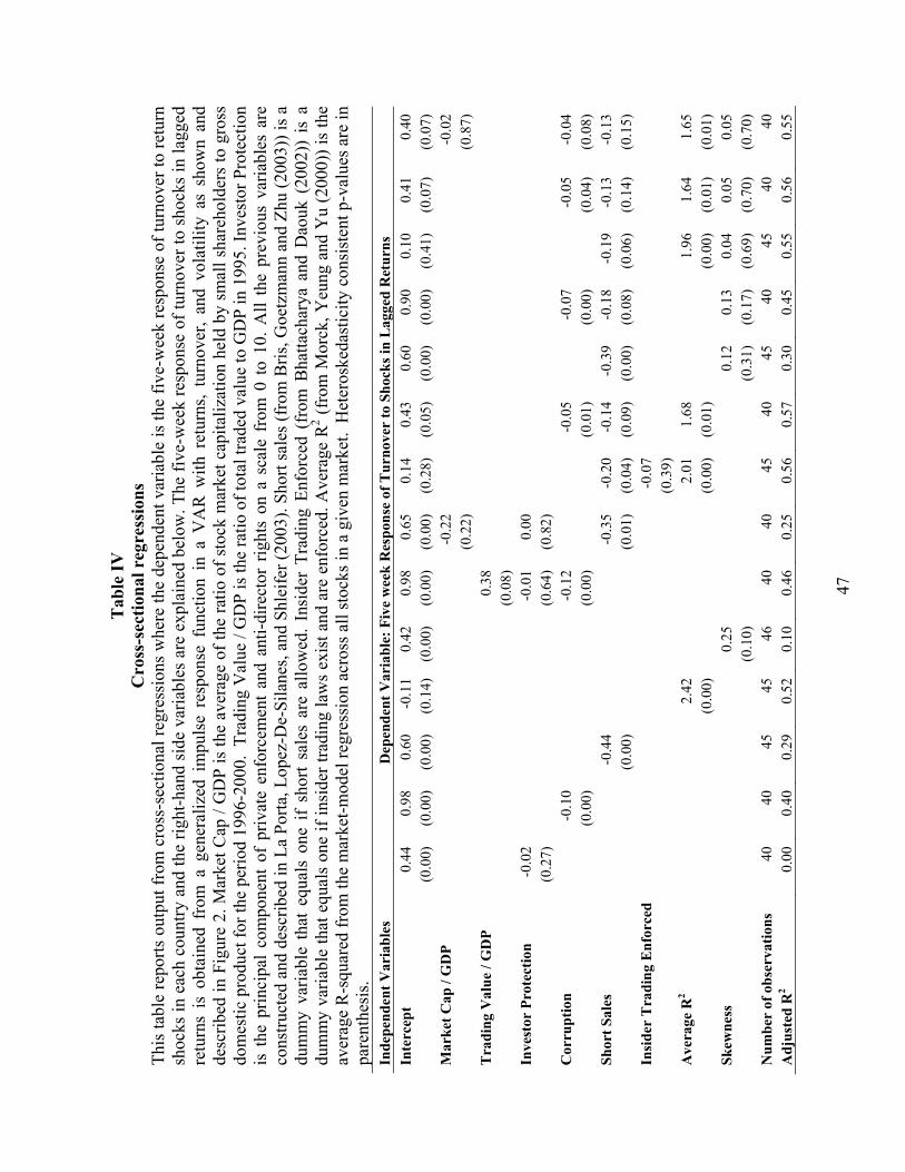
47

Tab

le IV

C

ross

-sec

tiona

l reg

ress

ions

Th

is ta

ble

repo

rts o

utpu

t fro

m c

ross

-sec

tiona

l reg

ress

ions

whe

re th

e de

pend

ent v

aria

ble

is th

e fiv

e-w

eek

resp

onse

of t

urno

ver t

o re

turn

sh

ocks

in e

ach

coun

try a

nd th

e rig

ht-h

and

side

var

iabl

es a

re e

xpla

ined

bel

ow. T

he fi

ve-w

eek

resp

onse

of t

urno

ver t

o sh

ocks

in la

gged

re

turn

s is

obt

aine

d fr

om a

gen

eral

ized

im

puls

e re

spon

se f

unct

ion

in a

VA

R w

ith r

etur

ns,

turn

over

, an

d vo

latil

ity a

s sh

own

and

desc

ribed

in F

igur

e 2.

Mar

ket C

ap /

GD

P is

the

aver

age

of th

e ra

tio o

f sto

ck m

arke

t cap

italiz

atio

n he

ld b

y sm

all s

hare

hold

ers

to g

ross

do

mes

tic p

rodu

ct fo

r the

per

iod

1996

-200

0. T

radi

ng V

alue

/ G

DP

is th

e ra

tio o

f tot

al tr

aded

val

ue to

GD

P in

199

5. In

vest

or P

rote

ctio

n is

the

prin

cipa

l co

mpo

nent

of

priv

ate

enfo

rcem

ent

and

anti-

dire

ctor

rig

hts

on a

sca

le f

rom

0 t

o 10

. All

the

prev

ious

var

iabl

es a

re

cons

truct

ed a

nd d

escr

ibed

in L

a Po

rta, L

opez

-De-

Sila

nes,

and

Shle

ifer (

2003

). Sh

ort s

ales

(fro

m B

ris, G

oetz

man

n an

d Zh

u (2

003)

) is a

du

mm

y va

riabl

e th

at e

qual

s on

e if

shor

t sa

les

are

allo

wed

. Ins

ider

Tra

ding

Enf

orce

d (f

rom

Bha

ttach

arya

and

Dao

uk (

2002

)) i

s a

dum

my

varia

ble

that

equ

als

one

if in

side

r tra

ding

law

s ex

ist a

nd a

re e

nfor

ced.

Ave

rage

R2 (f

rom

Mor

ck, Y

eung

and

Yu

(200

0)) i

s th

e av

erag

e R

-squ

ared

from

the

mar

ket-m

odel

regr

essi

on a

cros

s all

stoc

ks in

a g

iven

mar

ket.

Het

eros

keda

stic

ity c

onsi

sten

t p-v

alue

s are

in

pare

nthe

sis.

Inde

pend

ent V

aria

bles

D

epen

dent

Var

iabl

e: F

ive

wee

k R

espo

nse

of T

urno

ver

to S

hock

s in

Lag

ged

Ret

urns

In

terc

ept

0.44

0.

98

0.60

-0

.11

0.42

0.

98

0.65

0.

14

0.43

0.

60

0.90

0.

10

0.41

0.

40

(0

.00)

(0

.00)

(0

.00)

(0

.14)

(0

.00)

(0

.00)

(0

.00)

(0

.28)

(0

.05)

(0

.00)

(0

.00)

(0

.41)

(0

.07)

(0

.07)

M

arke

t Cap

/ G

DP

-0.2

2

-0

.02

(0

.22)

(0

.87)

T

radi

ng V

alue

/ G

DP

0.

38

(0.0

8)

Inve

stor

Pro

tect

ion

-0.0

2

-0

.01

0.00

(0

.27)

(0

.64)

(0

.82)

Cor

rupt

ion

-0

.10

-0

.12

-0.0

5

-0.0

7

-0.0

5 -0

.04

(0.0

0)

(0

.00)

(0

.01)

(0.0

0)

(0

.04)

(0

.08)

Sh

ort S

ales

-0

.44

-0

.35

-0.2

0 -0

.14

-0.3

9 -0

.18

-0.1

9 -0

.13

-0.1

3

(0.0

0)

(0

.01)

(0

.04)

(0

.09)

(0

.00)

(0

.08)

(0

.06)

(0

.14)

(0

.15)

In

side

r T

radi

ng E

nfor

ced

-0

.07

(0.3

9)

Ave

rage

R2

2.

42

2.

01

1.68

1.

96

1.64

1.

65

(0.0

0)

(0

.00)

(0

.01)

(0

.00)

(0

.01)

(0

.01)

Sk

ewne

ss

0.25

0.

12

0.13

0.

04

0.05

0.

05

(0

.10)

(0

.31)

(0

.17)

(0

.69)

(0

.70)

(0

.70)

N

umbe

r of

obs

erva

tions

40

40

45

45

46

40

40

45

40

45

40

45

40

40

A

djus

ted

R2

0.00

0.

40

0.29

0.

52

0.10

0.

46

0.25

0.

56

0.57

0.

30

0.45

0.

55

0.56

0.

55

48

Tab

le V

19

83-1

992

peri

od a

nd A

sym

met

ries

W

e es

timat

e w

eekl

y tri

varia

te V

AR

s of

det

rend

ed tu

rnov

er, r

etur

ns, a

nd v

olat

ility

. Det

rend

ed tu

rnov

er a

nd E

GA

RC

H (1

,1) v

olat

ility

ar

e ca

lcul

ated

as

desc

ribed

in F

igur

e 2.

Pan

el A

pre

sent

s su

mm

ary

stat

istic

s fo

r th

e G

IRF

for

the

Janu

ary

2, 1

983

to D

ecem

ber

31,

1992

per

iod

with

the

full

sam

ple.

Pan

el B

repo

rts re

sults

exc

ludi

ng th

e w

eek

of O

ctob

er 1

9, 1

987.

For

the

VA

Rs

in P

anel

C a

nd D

we

sepa

rate

ly c

ompu

te th

e G

IRF

for p

ositi

ve a

nd n

egat

ive

retu

rn s

hock

s. Pa

nel C

repo

rts th

e Th

resh

old

VA

R re

sults

for t

he 1

993-

2003

pe

riod

with

sep

arat

e re

spon

ses

to p

ositi

ve a

nd n

egat

ive

retu

rn s

hock

s w

hile

Pan

el D

is f

or th

e 19

83-1

992

perio

d. A

ll re

spon

ses

are

stan

dard

ized

by

the

estim

ated

res

idua

l va

rianc

e. T

he t

able

rep

orts

the

mea

n (µ

), m

edia

n (M

ed)

and

stan

dard

dev

iatio

n (σ

) of

the

re

spon

ses

for

high

-+in

com

e, d

evel

opin

g, a

nd a

ll co

untri

es.

We

also

rep

ort

the

num

ber

of p

ositi

ve (

+),

nega

tive

(-),

sign

ifica

ntly

po

sitiv

e (+

(*))

, and

sign

ifica

ntly

neg

ativ

e (-

(*))

resp

onse

s.

Hig

h In

com

e D

evel

opin

g A

ll C

ount

ries

G

IRF

µ M

ed

σ -

+

- (*)

+

(*)

µ M

ed

σ -

+

- (*)

+

(*)

µ M

ed

σ -

+

- (*)

+

(*)

Pane

l A: 1

983-

92 T

riva

riat

e V

AR

(In

clud

es '8

7 cr

ash)

L

ag 1

0.

12

0.12

0.

08

1 17

0

6 0.

36

0.35

0.

10

0 6

0 6

0.18

0.

16

0.14

1

23

0 12

L

ag 5

0.

43

0.42

0.

28

1 17

0

11

1.19

1.

24

0.44

0

6 0

6 0.

62

0.55

0.

46

1 23

0

17

Lag

10

0.52

0.

55

0.37

1

17

0 10

1.

31

1.34

0.

52

0 6

0 6

0.72

0.

70

0.53

1

23

0 16

Pa

nel B

: 198

3-92

Tri

vari

ate

VA

R (

Exc

lude

s '87

cra

sh)

Lag

1

0.15

0.

15

0.08

1

17

0 9

0.37

0.

36

0.09

0

6 0

6 0.

21

0.17

0.

13

1 23

0

15

Lag

5

0.49

0.

43

0.27

1

17

0 14

1.

26

1.26

0.

38

0 6

0 6

0.68

0.

65

0.45

1

23

0 20

L

ag 1

0

0.57

0.

50

0.35

1

17

0 14

1.

40

1.43

0.

45

0 6

0 6

0.78

0.

75

0.52

1

23

0 20

Pa

nel C

: 199

3 -2

003

Res

pons

e of

Tur

nove

r to

Pos

itive

and

Neg

ativ

e R

etur

n Sh

ocks

Po

s Lag

10

0.28

0.

21

0.33

5

21

- -

0.61

0.

52

0.38

1

19

- -

0.43

0.

44

0.39

6

40

- -

Neg

Lag

10

-0.2

9 -0

.18

0.33

24

2

- -

-0.6

8 -0

.62

0.40

20

0

- -

-0.4

6 -0

.43

0.41

44

2

- -

Pane

l D: 1

983-

1992

Res

pons

e of

Tur

nove

r to

Pos

itive

and

Neg

ativ

e R

etur

n Sh

ocks

Po

s Lag

10

0.56

0.

54

0.31

1

17

- -

1.28

1.

24

0.39

0

6 -

- 0.

74

0.72

0.

45

1 23

-

- N

eg L

ag 1

0 -0

.59

-0.5

9 0.

33

17

1 -

- -1

.21

-1.1

6 0.

37

6 0

- -

-0.7

4 -0

.74

0.43

23

1

- -