nber working paper series solving externalities by incenting workers directly · 2016-06-17 ·...

NBER WORKING PAPER SERIES

A NEW APPROACH TO AN AGE-OLD PROBLEM:SOLVING EXTERNALITIES BY INCENTING WORKERS DIRECTLY

Greer K. GosnellJohn A. List

Robert Metcalfe

Working Paper 22316http://www.nber.org/papers/w22316

NATIONAL BUREAU OF ECONOMIC RESEARCH1050 Massachusetts Avenue

Cambridge, MA 02138June 2016

We thank participants at the 2015 EEE and PPE NBER Summer Institute sessions for excellent remarks that considerably improved the research, and seminar participants at Columbia University, Dartmouth College, University of British Columbia, University of Chicago, University of Tennessee, and University of Wisconsin-Madison. Omar Al-Ubaydli, Steve Cicala, Diane Coyle, Paul Dolan, Robert Dur, Robert Hahn, Glenn Harrison, Justine Hastings, David Jimenez-Gomez, Matthew Kahn, Kory Kroft, Edward Lazear, Steve Levitt, Bentley MacLoed, Jonathan Meer, Michael Norton, Sally Sadoff, Laura Schechter, Jessie Shapiro, Kathryn Shaw, Kerry Smith, Alex Teytelboym, Gernot Wagner, and Catherine Wolfram provided remarks that helped to sharpen our thoughts. Thanks to The Templeton Foundation and the Science of Philanthropy Initiative at the University of Chicago for providing the generous funds to make this experiment possible. Further thanks to the UK Civil Aviation Authority and the pilots’ unions who took the time to review and approve of the study objectives and material. A special thanks to those individuals at Virgin Atlantic Airways—especially to Paul Morris, Claire Lambert, Emma Harvey, and Captain David Kistruck—and Rolls Royce (especially Mark Goodhind and Simon Mayes) for their essential roles in the implementation of this experiment. These parties are in no way responsible for the analyses and interpretations presented in this paper. We thank Florian Rundhammer and Andrew Simon for their excellent research assistance. The views expressed herein are those of the authors and do not necessarily reflect the views of the National Bureau of Economic Research.

NBER working papers are circulated for discussion and comment purposes. They have not been peer-reviewed or been subject to the review by the NBER Board of Directors that accompanies official NBER publications.

© 2016 by Greer K. Gosnell, John A. List, and Robert Metcalfe. All rights reserved. Short sections of text, not to exceed two paragraphs, may be quoted without explicit permission provided that full credit, including © notice, is given to the source.

A New Approach to an Age-Old Problem: Solving Externalities by Incenting Workers DirectlyGreer K. Gosnell, John A. List, and Robert MetcalfeNBER Working Paper No. 22316June 2016JEL No. D01,J3,Q5,R4

ABSTRACT

Understanding motivations in the workplace remains of utmost import as economies around the world rely on increases in labor productivity to foster sustainable economic growth. This study makes use of a unique opportunity to “look under the hood” of an organization that critically relies on worker effort and performance. By partnering with Virgin Atlantic Airways on a field experiment that includes over 40,000 unique flights covering an eight-month period, we explore how information and incentives affect captains’ performance. Making use of more than 110,000 captain-level observations, we find that our set of treatments—which include performance information, personal targets, and prosocial incentives—induces captains to improve efficiency in all three key flight areas: pre-flight, in-flight, and post-flight. We estimate that our treatments saved between 266,000-704,000 kg of fuel for the airline over the eight-month experimental period. These savings led to between 838,000-2.22 million kg of CO2 abated at a marginal abatement cost of negative $250 per ton of CO2 (i.e. a $250 savings per ton abated) over the eight-month experimental period. Methodologically, our approach highlights the potential usefulness of moving beyond an experimental design that focuses on short-run substitution effects, and it also suggests a new way to combat firm-level externalities: target workers rather than the firm as a whole.

Greer K. GosnellLondon School of Economicsand Political [email protected]

John A. ListDepartment of EconomicsUniversity of Chicago1126 East 59thChicago, IL 60637and [email protected]

Robert MetcalfeUniversity of ChicagoSaieh Hall for Economics5757 S. University AvenueChicago IL, [email protected]

1 Introduction

Many scientists believe that global climate change represents the most pervasive externalityof our time (Stern, 2006). Perhaps one of the lowest-hanging fruits in combating climatechange is to design firm-level incentive schemes for workers to engage in green behaviors.We are not aware of any studies that have explored incentive aspects within the workplacethat pertain to sustainability, whether it is shifting work hours to less energy-intensive timesof the day or incenting employees to use fewer resources per unit of output. Given theEnvironmental Protection Agency estimate that 21 percent of carbon emissions in the UnitedStates are from firms (U.S. Enviromental Protection Agency, 2015), there is undoubtedlymuch to gain. Indeed, when resource use is linked to production costs (as is almost alwaysthe case), mitigating the externality has the potential to foster increased profits, providingdistinct possibilities of a win-win scenario.

Consider the transportation sector, and in particular air transportation of humans andcargo. The airline industry is a significant contributor to human welfare, with over threebillion passengers per year and 35% of the value of world trade transported by air (FederalAviation Administration, 2015). However, the global aviation industry is directly responsi-ble for significant health costs among vulnerable population groups (Schlenker and Walker,2015).1 Moreover, excessive fuel use in the industry affects profits—fuel represents an aver-age 33% of operating costs (Air Transport Action Group, 2014)—and poses a severe risk tothe global environment. Emissions from the air transport sector currently account for 3.5-5%of global radiative forcing and 2-3% of global carbon dioxide emissions (Penner et al., 1999;Lee et al., 2009; Burkhardt and Kärcher, 2011), deeming the industry a significant force inclimate change discussions.2 Technology adoption and market-based instruments continue toappear on the industry’s agenda as primary means to reach its dual goals of carbon neutralgrowth by 2020 and halving greenhouse gas emissions from 2005 levels by 2050 (see Inter-national Civil Aviation Organization, 2013). Yet, despite large potential to reduce fuel burnfrom eliminating operational inefficiencies (Green, 2009; Singh and Sharma, 2015), almost

1Schlenker and Walker (2015) focus on the effects of network delays in the east coast of the United Stateson congestion at large airports in California to assess health effects from daily variation in air pollution.These effects are presumed to be generalizable across large airports globally and are a consequence of theaviation industry as a whole.

2Past research has shown that the airline industry has also not fully internalized social costs associatedwith crashes (Borenstein and Zimmerman, 1988). Here we highlight yet another means by which the socialcost of the industry is not incorporated into its decision calculus. Nonetheless, demand for air travel isforecasted to increase over the next two decades and, as a result, airline emissions will likely trend upwards(Borenstein, 2011).

1

no research has been undertaken to understand the potential for cost and emissions savingsfrom changes in the behavior of transport personnel. In fact, we do not know of any research,more generally, on the optimal incentive structure for employees to engage in conservationactivities in the workplace.

Our study takes a strong initial step toward such an understanding by partnering withVirgin Atlantic Airways (VAA) on a field experiment. We observe over 40,000 unique flightsover a 27-month period for the entire population of captains eligible to fly both before andduring the experiment.3 In the aviation industry, airline captains maintain a considerableamount of autonomy when it comes to fuel and flight decisions.4 We capitalize on recenttechnological developments that capture detailed flight-level data to measure captains’ fuelefficiency across three distinct phases—pre-flight, in-flight, and post-flight.5 Our pre-flightmeasure (denoted Fuel Load) assesses the accuracy with which captains implement finaladjustments to aircraft fuel load given all relevant factors (e.g., weather and aircraft weight).Our in-flight measure (denoted Efficient Flight) assesses how fuel-efficiently the captainoperates the aircraft between takeoff and landing. Our post-flight measure (denoted EfficientTaxi) provides information on how fuel-efficiently the captain operates the aircraft once onthe ground.

Our experiment explores the extent to which several experimental treatments—implemen-ted from February 2014 through September 2014—influence captains’ behaviors. The treat-ments are inspired by a simple principal-agent model wherein we attempt to influence thebehaviors of VAA captains. Our theoretical model yields predictions on how the act ofmeasurement itself might yield behavioral change, in the spirit of the Hawthorne effects

3The “captain”—as opposed to the “first officer”—is the pilot on the aircraft who makes commanddecisions and is ultimately responsible for the flight’s safety. As a rule, captains are the most senior pilots inan airline (see Smith (2013) for insight into captains’ roles and responsibilities). In the cockpit of a typicalflight from New York to London, there would be one captain and one first officer on board who both engage(more or less equally) in aircraft operations, though the captain is ultimately responsible for all aspects offlight operation. A vast majority of airline captains survive rigorous job market competition to secure theirjobs, investing thousands of hours of training (privately or elsewhere) before obtaining the opportunity tobe considered for a flying career with a major airline. A handful of VAA captains who were on leave forpersonal reasons or were fulfilling duties outside of their usual obligations were excluded from the sample.

4There has been prior research on understanding the decision making of airline captains under risk,especially through weather conditions (see Gilbey and Hill, 2012; Hunter, 2002; Madhavan and Lacson,2006; Walmsley and Gilbey, 2016; Wiggins et al., 2012).

5The Fuel Efficiency team within Virgin Atlantic Airways was responsible for identification of the fuel-efficient behaviors targeted in this study, which represent the outcomes of just a few of the many decisionsthat a captain engages with during a given flight.

2

described in Levitt and List (2011).6 In addition, the model shows how performance infor-mation, personal targets, and prosocial incentives for reaching those targets can motivatebehavioral change. As such, our experimental design revolves around understanding howthe act of measurement and each of these three factors—information about recent fuel effi-ciency, information including target fuel usage, and prosocial incentives (a donation to thecaptain’s chosen charity conditional on achieving the target efficiency)—affect captains’ be-haviors from pre-flight to post-flight. We are unaware of any previous research that teststhe impacts of targets or prosocial incentives on worker productivity in such a high-stakesprofessional setting.

Making use of more than 110,000 observations of behavior across 335 captains, we findseveral interesting insights that have the potential to alter conventional approaches to mo-tivate employee effort in the workplace and to both efficiently reduce operating costs andenvironmental waste. Perhaps most surprisingly, by simply informing the captains that we—i.e. the academic researchers and VAA Fuel Efficiency personnel overseeing the study—aremeasuring their behaviors on three dimensions, we are able to considerably reduce fuel ineffi-ciency.7 For example, captains significantly increased the implementation of Efficient Flightand Efficient Taxi by nearly 50 percent from the pre-experimental period. These behav-ioral changes generated more than 6.8 million kilograms of fuel saved for the airline overthe eight-month experimental period (i.e. $5.37 million in fuel savings), which translated to

6Captains were assured on several occasions that their participation in the experiment held no implicationsor consequences for their salaries or career prospects. For instance, the initial letter sent to all (treatmentand control) captains in January 2014 included the following statements (emphasis included): “This isnot, in any way, shape or form, an attempt to set up a ‘fuel league table’, or any attempt atmoving in the direction of a fuel league table. It is an independent research project to see whetherinformation provided in different ways affects individual decisions. All data gathered during this study willremain anonymous and confidential... Again, we would like to stress that Captains’ anonymity will bemaintained throughout the study; whilst somebody in Flight Ops Admin has to correlate which Captain getswhich letter, Flight Operations Management will have no visibility of which Captain is in which Group, andwho is doing what in response to which information. Information will be sent to all Captains in the activestudy groups. What you choose to do with that information is entirely up to you.”

7This pure monitoring effect aligns with agency theory (e.g., Alchian and Demsetz, 1972; Stiglitz, 1975),as well as with experimental results such as those in Boly (2011). These results are also related to the workof Hubbard (2000, 2003), who found that monitoring truckers’ performance using GPS technology leads toimproved performance for those workers where driver effort is important and where verifying drivers’ actionsto insurers is valuable. He estimates that such technology has increased capacity utilization by around 3%in the trucking industry. Company policies precluded the designation of an uninformed control group, soestimates of Hawthorne effects are based on before-and-after comparisons, as in Bandiera et al. (2007, 2009).Nonetheless, our results suggest that the data before the experiment was stationary and there was an upwardtrend once the experiment started (adjusting for seasonality). Importantly, since all information providedto captains in treatment groups is individual-specific, we are able to rule out contamination (i.e. spillovereffects of information) as a possible contributor to the change in behavior exhibited by the control group.

3

more than 21 million kg of CO2 abated.Despite these large Hawthorne effects, we find a significant role for our three experimen-

tal treatments. Our information treatment increases effort for Efficient Taxi, but does notincrease effort for Fuel Load or Efficient Flight. We find, however, that personal targetsincrease effort for Efficient Flight and Efficient Taxi. Finally, prosocial incentives increaseeffort across all three dimensions. Furthermore, we find significant differences between infor-mation and the two other treatments while we do not detect differential effects between thetarget and prosocial treatment groups. That is, adding conditional prosocial incentives inthe form of a donation to the captain’s chosen charity does not provide further lift beyondthe effects of a personal target.8 Yet, there is an interesting effect of prosocial incentives:they induce a reduction in flying time by an average of 1 minute and 30 seconds per flightrelative to the control group, equivalent to more than 80 hours of reduced flight time overthe eight-month course of the study.9

Our difference-in-difference treatment effect estimates indicate that the various inter-ventions increased implementation of fuel-efficient activities by 1-10 percent above the pre-experimental period (i.e. in addition to the Hawthorne effect).10 Based on these effects, weestimate that our three treatments saved between 266,000-704,000 kg ($209,000-$553,000) offuel for the airline over the eight-month experimental period. This fuel savings correspondsto 838,000-2,220,000 kg of CO2 abated. Since the cost of the treatments is merely the costof postage materials (here, $855 per treatment group), the marginal abatement cost (MAC)of the treatments is minuscule, falling between $1.02 and $0.39 per ton of carbon saved.However, since the airline benefited from significant cost savings via reduced fuel usage as aresult of our interventions, the MAC in this context is -$250 per ton in actuality. Such anastonishingly low MAC outperforms every other reported carbon abatement technology ofwhich we are aware (see Enkvist and Rosander, 2007; McKinsey, 2009).11

Our experimental design highlights the usefulness of moving beyond short-run effects in8We believe that we are the first to experimentally estimate the impact of an incentive given to a charity

if the worker reaches a certain performance target in his or her job. Our notion of prosocial incentives istherefore different to the social incentives presented in Bandiera et al. (2009, 2010).

9These results are based on all flights and are presented in Table A7. The total is obtained by multiplyingthe average effect of captains in the prosocial treatment group relative to control by the number of flightsundertaken in the prosocial treatment group during the study period.

10Since there were no upward trends before the experiment began—that is, a Dickey-Fuller test indicatesthat pre-treatment behaviors were stationary—we can be certain that our experiment improved fuel efficiencyfrom business as usual.

11The most cost-effective abatement strategy according to McKinsey (2009) is switching residential lightingfrom incandescent bulbs to LED bulbs at a MAC of approximately -165 Euro, or about -$177.

4

favor of understanding long-term embedded behavior change. First, in terms of persistenceof the treatment effects throughout the experiment, we find that the largest effects for FuelLoad and Efficient Flight arise in the middle months of the experiment, while the treat-ment effect for Efficient Taxi is consistently high throughout the experiment. Interestingly,across all three treatments, we find the largest effects for the behavior that is the easiest tochange (Efficient Taxi). Once the experiment finishes, however, we find that captains’ effortreverts to post-experiment baseline levels (i.e. equivalent attainment to the control grouponce the experiment terminates) for Fuel Load and Efficient Flight, though the treatmenteffects remain for Efficient Taxi. With regards to the persistence of the Hawthorne effect, thepost-experiment baseline remains considerably improved from the pre-experiment baseline,perhaps indicating that monitoring induces captains to make low-effort efficiency improve-ments that are quickly and easily habituated. A different interpretation to the Hawthorneeffect could be that the Captains now learn that the firm values fuel efficiency (which theCaptains probably also believe is a good thing). This relates to the work by Bloom andVan Reenen (2007) and Bloom et al. (2014) on the impact of ‘soft’ management styles andstructures on worker productivity.

Finally, our design allows us to demonstrate welfare benefits pertaining to the employees.We find that captains’ job satisfaction is positively influenced by prosocial incentives andjob performance. Captains in the prosocial treatment group report a job satisfaction rating6.5% higher than captains in the control group. Moreover, for every additional personaltarget met by captains receiving targets or prosocial incentives (out of 24 opportunities intotal), job satisfaction increases by 1%, on average. Based on this result, we therefore notonly encourage airlines to provide captains with performance-based targets to improve fuelefficiency, but also urge them to discover means by which to support captains in reachingsaid targets in order to improve their well-being.12

Our findings are important for academics, businesses, and policymakers alike. For aca-demics, the theory and experimental results hold implications for environmental, behavioral,labor, and public economics. For example, there exist movements within both applied eco-nomics (“X-efficiency”; see Leibenstein, 1966) and environmental economics (the “PorterHypothesis”; see Porter and van der Linde, 1995) arguing that substantial “free gains” existwithin firms. The premise is a behavioral one: rather than modeling firms as fully aware andunderstanding of all extant means to maximize resource efficiency—thereby exhausting all

12While we are dubious of using subjective assessments of well-being as precise measurements of welfare,we measured job satisfaction in our survey since it is a metric commonly used in the airline and otherindustries to assess the well-being of employees.

5

cost-efficient measures at each moment in time—this approach considers the firm as a compo-sition of networks of boundedly rational individuals burdened by problematic principal-agentincentive conflicts (Leibenstein, 1966; Perelman, 2011). To support this view, a survey ofevidence argues that a typical firm operates at 65% to 97% efficiency (Button and Weyman-Jones, 1992), though much of this evidence is based on observational data and does notassess impacts based on a true counterfactual. Our work complements this environmentaland behavioral research by moving in a hitherto unconsidered direction: rather than focuson capital improvements or research and development, we explore efficiency effects of in-centing labor directly during their normal course of work. For labor economists consideringprincipal-agent settings, our study suggests that allowing the agent flexibility to achievegoals might be a key trigger in enhancing effort profiles.13

For businesses and policymakers, we present a novel and promising approach to combat-ing firm-level externalities: design appropriate incentives for workers. More narrowly, thestudy provides practical and cost-effective fuel solutions for the air transport industry. Ourempirical approach lends itself naturally to related tests across other sectors of the economy.By making use of our theoretical framework to guide experimental treatments in the field,businesses and policymakers can learn not only what works, but also why it works. Thisunderstanding will provide decision-makers with a more effective toolkit to advance efficientpolicies and procedures.

The remainder of our paper is structured as follows. Section 2 provides background,a sketch of the theory, and the experimental design. Section 3 presents the experimentalresults. Section 4 provides a discussion related to policy implications and related avenuesfor future research.

2 Background, Theory, and Experimental Design

A few years ago we began discussions with VAA to partner on a field experiment withthe aim of understanding behavioral components of fuel usage without adversely affecting

13This leads to another unique feature of the study which is that we are not in a typical principal-agentproblem in which the principal does not observe effort. Here, the principal has very good measures ofeffort. Instead, the principal has contractual restrictions (from the union) against contracting on effort (oron output), which is the typical contracting variable in a basic principal-agent model. Instead, the firm isin a “second-best” world of needing to use behavioral incentives instead of financial incentives.

6

safety practices or job satisfaction.14 We developed a theoretical framework and a fieldexperiment (detailed further below) that allow us to remain within institutional constraintswhile maintaining the integrity of lending theoretical insights to the experimental data. Wewere permitted to provide monthly tailored feedback to 335 airline captains—the entireeligible captain population of VAA—from February 2014-September 2014. Importantly, alleligible VAA captains were included in the experiment—in either control or treatment. VAAcaptains have absolute authority to make all fuel decisions. They range in experience and flylong-haul flights on various aircraft types (Airbus 330-300, Airbus 340-300, Airbus 340-600,Boeing 744-400, Boeing 787-9). We include a map of destinations in Figure 1.15

While many of the captains’ choices are important in terms of fuel efficiency outcomes,VAA identified three primary measurable levers to change behavior for the purpose of thisstudy. The first lever is a pre-flight consideration, which VAA denotes as Zero Fuel Weight(ZFW) adjustment. Approximately 90 minutes before each flight, captains utilize flight-specific flight plan information (e.g., expected fuel usage, weather, and aircraft weight) inconjunction with their own professional judgment to determine initial fuel uptake, whichusually corresponds to approximately 90% of the anticipated fuel necessary for the flight.This amount is fueled into the aircraft simultaneous to the loading of passengers and cargo.Near to completion of passenger boarding and cargo/baggage loading, the pilots—now onthe flight deck—receive updated information regarding the final weight of the aircraft andmay adjust the fuel on the aircraft accordingly. The information they receive from FlightOperations includes a ZFW measure, which indicates the weight of the aircraft with therevenue load (i.e. passengers and cargo), as well as the Takeoff Weight (TOW), whichincludes both revenue load and fuel.

Captains then perform a ZFW calculation in which they first calculate the amount bywhich they should increase or decrease fuel load based on the final ZFW—a formula thatis standard across the airline industry. If they have chosen to increase the fuel load, theysubsequently compute a second iteration to account for the additional fuel necessary to carrythe fuel that they have chosen to add to the aircraft. If the amount of fuel already on theaircraft is sufficient according to these calculations, the captain may choose not to add anyadditional fuel.

14The study is a component of Change is in the Air, VAA’s wider sustainabil-ity initiative focused primarily on fuel and carbon reduction (see http://www.virgin-atlantic.com/content/dam/VAA/Documents/sustainabilitypdf/SustainabilityPolicy201407.05.14.pd).

15All operations to Aberdeen and Edinburgh are VAA Little Red operations (i.e. branded VAA flightsoperated by a third party) and were excluded from the analysis. In April 2015, VAA removed its service toCape Town; this route change took place subsequent to the period covered in our dataset.

7

http://www.virgin-atlantic.com/content/dam/VAA/Documents/sustainabilitypdf/SustainabilityPolicy2014_07.05.14.pdf

http://www.virgin-atlantic.com/content/dam/VAA/Documents/sustainabilitypdf/SustainabilityPolicy2014_07.05.14.pdf

For mnemonic purposes, rather than use ZFW we denote this binary outcome variableas Fuel Load. Fuel Load indicates whether this double iteration has been performed and thefuel level adjusted accordingly. We deem the captains’ behavior as successful if their finalfuel load is within 200 kg of the “correct” amount of fuel as dictated by the calculation. Thisallowance prevents penalizing captains for rounding and slight over- or under-fuelling on thepart of the fueller while providing measurable targets for captains in two of our treatmentgroups.16 According to our partner airline, accurate Fuel Load adjustment should ideallybe performed on every flight regardless of circumstances, which would correspond to 100%attainment for the performance metric provided.

The second lever is an in-flight consideration: Efficient Flight. The Efficient Flight metriccaptures whether captains (and their co-pilots) use less fuel during flight than is allotted inthe updated flight plan.17 We use this metric to understand whether captains have madefuel-efficient choices between takeoff and landing. This measure incorporates several in-flightbehaviors that augment fuel efficiency, such as requesting and executing optimal altitudesand shortcuts from air traffic control, maintaining ideal speeds, optimally adjusting to enroute weather updates, and ensuring efficient aerodynamic arrangements with respect toflap settings as well as takeoff and landing gear. We decided on Efficient Flight to measurein-flight efficiency since it is the only measure considered that affords captains the flexibilityto achieve the target while using professional judgment to ensure that safety remains thefirst priority. Under some uncommon circumstances, operational requirements dictate thatcaptains sacrifice fuel efficiency (and VAA accepts the captains’ decisions as final), so wewould not expect even a “model” captain to perform this metric on 100% of flights, thoughthe metric should be attainable on a vast majority of flights. In our analysis, Efficient Flightequals 1 if the captain does not exceed the projected fuel use for that flight (adjusted foractual TOW), and 0 otherwise.18

VAA’s final lever—reduced-engine taxi-in (Efficient Taxi or Efficient Taxiing, hereafter)—16Sustainable Aviation (2012, hereafter “SA”) estimates that more accurate fuel-loading can save approx-

imately 0.5% of total fuel burn; with average fuel consumption per flight of 69,500 kg, the correspondingfuel savings is approximately 350 kg fuel per flight. SA is an alliance of UK airlines, airports, aerospacemanufacturers, and air navigation service providers with the long-term objective of reducing air and noisepollution. Using data from its 2014 sectors, our partner airline estimated an average fuel savings of 250kg per sector for correct Fuel Load calculations. Ryerson et al. (2015) attempt to estimate the excess fuelburned for an anonymous airline by too much fuel being loaded onto the plane.

17The flight plan is updated subsequent to decisions made on Fuel Load so that decisions regarding thefirst metric do not affect one’s ability to meet this in-flight metric.

18We created binary variables for Fuel Load and Efficient Flight so we could assign targets to captains inthe targets and prosocial incentives group.

8

occurs post-flight. Once the aircraft has landed and the engines have cooled, captains maychoose to shut down one (or two, in a four-engine aircraft) of their engines while theytaxi to the gate, thereby decreasing fuel burn per minute spent taxiing. Captains meetthe criteria for this metric if they shut down (at least) one engine during taxi in.19 Aswith Efficient Flight, there are circumstances under which the airline would not expect orprescribe the implementation of Efficient Taxi. Obstacles include geographical constraints(e.g., the placement or layout of the runway) and the complexity of the taxi route (e.g.,number of stops, turns, or cul-de-sacs). Still, the metric should also be attainable on a vastmajority of flights, and obstacles to implementation are uncorrelated with treatment.

Fuel Load, Efficient Flight, and Efficient Taxi are the three primary outcome variables inour experiment. It is important to recognize that fuel is a major cost to airlines—accountingfor roughly 33 percent20 of total operating costs—and has been rising over the last fifteenyears (Borenstein, 2011; International Air Transport Association, 2014). For this reasonairlines are interested in cost-effective means to reduce fuel burn per flight. Given theirrenowned expertise and experience in the industry, however, airline captains are granted sig-nificant autonomy in their decision-making across several fuel-relevant behaviors, includingthose described above. Moreover, airline captains are unionized so it is contractually difficultto use performance-related pay to motivate fuel efficiency.21 As such, we focus on airlinecaptains’ behavioral adjustments to reduce fuel usage.

Theoretical Sketch of Captains’ Behavior

We model an airline captain’s choices using a static game of a principal-agent model thatdetermines a captain’s chosen effort in a given period (for parsimony, we briefly sketch themodel here and provide details in Appendix II). The tasks consist of the aforementioned pre-flight to post-flight fuel usage metrics. Captains observe their own effort and a signal of fuelusage; the signal is noisy unless the captain receives information. Captain’s perspectives onfuel usage and their fuel-relevant decisions are rooted in their own experiences and preferencesand are conditional on contextual (i.e. flight- and day-specific) factors.

19SA estimates that this practice—in conjunction with reduction in auxiliary power use substitution—prevents the emissions of 100,000 metric tons of CO2 annually. Fuel savings from Efficient Taxi depend onscheduling and delays as savings are accrued on a per-minute basis. Fuel savings also depend on aircrafttype and only begin to accrue after engines have cooled, which takes 2-5 minutes from touch down. Savingsper minute for aircraft operated within our study are as follows: 12.5 kg (B744, A330), 8.75 kg (A346), and6.25 kg (A343).

20For the airline represented in this study, fuel accounts for 35% of operating costs.21For a discussion of how unionization can affect the long-run outcomes of firms, see Lee and Mas (2012).

9

Captains choose how much effort to exert to maximize a utility function that includesutility from wealth, job performance, and charitable giving, as well as disutility from effortexertion and social pressure. The model has the standard prediction from the first orderconditions that the captain will expand effort until its marginal cost equals the marginalutility gained from the associated decrease in fuel usage. This prediction occurs on severaldimensions, such as utility from job performance, utility from giving to a charity, as well asdisutility from social pressure (a la DellaVigna et al. (2012)).

Although our base model follows DellaVigna et al. (2012), we extend the model to in-corporate a reference-dependent component to capture the effects of exogenous targets. Inline with existing theories of reference dependence, we posit that a change in one’s per-sonal expectations from the status quo to an improved outcome can boost performance and,consequently, utility. We therefore introduce feedback to employees providing non-bindingtargets—i.e. focal points for attainment of the three fuel-relevant behaviors—that encapsu-late reference-dependent preferences.22 We expect utility from job satisfaction to increasefor those who meet their targets. As in the Köszegi and Rabin (2006) model of reference-dependent preferences, we assume individuals are loss averse and, as such, performing belowthe target level will cause more disutility than exceeding the target level will benefit theindividual.

The notion that prosocial incentives can motivate behavior change is rooted in theoriesof pure and impure altruism (Becker, 1974; Andreoni, 1989, 1990). Pure altruism requiresthat individuals derive utility from the benefits they directly receive from the provision ofa public good. Impure altruism posits that individuals gain utility from the act of givingitself, so that an individual whose altruism is completely impure will provide the same dollarvalue toward the public good regardless of the provision of others. Both pure and impurealtruism provide positive utility to (altruistic) economic agents, and we assume that indi-viduals are characterized by some combination of the two (we do not attempt to distinguish

22There is a rich psychology literature on goal setting. Heath et al. (1999) present evidence that goals actas reference points inducing loss aversion and diminishing sensitivity in a manner consistent with ProspectTheory. Additionally, Locke and Latham (2006, p. 265) argue that psychology studies show that “specific,high (hard) goals lead to a higher level of task performance than do easy goals or vague, abstract goals such asthe exhortation to ‘do one’s best.”’ According to this line of research, there are four factors that determine theeffectiveness of the target, namely feedback (which people need in order to track their progress); commitmentto the goal (which is enhanced by self-efficacy and viewing the goal as important); task complexity (to theextent that task knowledge is harder to acquire on complex tasks); and situational constraints. Clearly,within our experiment, we provide feedback on a monthly basis, though the experiment is characterizedby individual-level differences in task complexity, absence of prior commitments, and a very high-stakescontext. Psychology studies do not exist that address the complex and high-stake field environment in whichour experiment takes place.

10

between them in our experiment). This characterization provides a prediction that altruisticmotivations combined with charitable incentives will augment fuel efficiency.

In equilibrium, captains choose the corresponding effort level that satisfies the first orderconditions. These choices lead to several propositions.23 First, if social pressure is important,then captains in the control group will improve their fuel efficiency due to the enhancedscrutiny of their fuel usage. Second, providing information to captains will cause them toincrease (weakly decrease) their effort if estimated fuel usage is lower (higher) than theiractual fuel usage. The intuition is that the relationship between captains’ estimated fuelusage and their actual fuel usage importantly determines their utility from job satisfaction.For example, informing captains that they are fuel inefficient will induce captains to exertgreater effort if they derive disutility from consuming more fuel than their estimated usage.Alternatively, if their fuel usage is deemed lower than their estimated usage, they mightexert less effort since effort is costly.

Third, targets set above pre-study fuel use will cause captains to weakly increase theireffort.24 Captains will increase their effort if the marginal gain from the associated decreasein fuel usage due to the target is greater than the marginal cost of effort. Alternatively,captains will not increase their effort if the marginal cost of effort is larger than the marginalgain from the associated decrease in fuel usage in the job satisfaction parameter. Fourth,conditional donations to charity will increase effort if captains’ altruism is strictly positiveand will not affect their effort otherwise. Fifth, of the three dimensions to lower fuel usage—pre-flight, in-flight, and post-flight—captains will choose to increase their effort the most intasks for which the targets are least costly to meet (i.e. Efficient Taxi).

In light of these predictions, we design a field experiment to measure how behaviors re-lated to fuel usage are affected by: i) information about recent fuel efficiency, ii) informationabout target fuel efficiency, and iii) a donation to a chosen charity conditional on achiev-ing the target efficiency. To our knowledge, we are the first to perform a large-scale fieldexperiment on firm employees in a real-world extremely high-stakes labor setting (where

23These propositions would be the same if we set up the model in the vein of a multi-tasking model.24All targets were set by the firm to improve on the pre-study outcomes, so this is the only case we

consider.

11

the average salary of a captain is roughly $175,000-$225,00025).26 In doing so, we overcomeprominent labor market frictions in the airline industry by implementing interventions thatdo not change contracts of the captains.27 We outline the field experimental design below.

Experimental Design

In accordance with our theoretical model, our field experiment focuses on three mainbehavioral motivations for optimizing fuel use: impacts of personalized information, perfor-mance targets, and prosocial incentives. The three treatments targeted three main behaviorsrelevant to fuel use: Fuel Load, Efficient Flight, and Efficient Taxi. Respectively, these threebehaviors allow us to capture captains’ behavior before takeoff, during the flight, and afterlanding. Airline captains did not receive detailed information relating their decision-makingto their fuel efficiency prior to this experiment (consistent with both airline and industrystandards). Recent advances in aircraft data collection allow us to obtain precise data toinform captains of the link between their effort and their efficiency.

25This salary range is based on information updated in June 2015:http://www.pilotjobsnetwork.com/jobs/Virgin_Atlantic.

26There is a growing literature surrounding field labor economics, but most experiments have focused onsimple tasks (List and Rasul, 2011; Bandiera et al., 2011; Levitt and Neckermann, 2014). Bandiera et al.(2007, 2009, 2010), using a before and after design within the same company, demonstrate the effects ofmanagerial compensation and social connections in the workplace on worker productivity and selection in thefruit picking industry. Shearer (2004) finds that piece-rate wages improve worker productivity in tree plantingrelative to fixed-rate wages; Lazear (1999) finds similar incentive effects of piece-rate wages in an observationalstudy of automobile glass installers. Field experiments on the impact of retail store-level tournaments onsales show mixed results (Delfgaauw et al., 2013, 2014, 2015), while a quasi-experiment showed that simplyinforming warehouse employees of relative wage standing permanently improved productivity (Blanes i Vidaland Nossol, 2011). One exception to such task simplicity is Gibbs et al. (2014), who analyze the effects ofa rewards program on innovation at a large Asian technology firm in a field experimental setting. Theyfind that providing rewards for idea acceptance substantially increases the quality of ideas submitted. Inan envelope-stuffing experiment, Al-Ubaydli et al. (2015) find that quality is actually higher under piece-rate wages (contrary to predictions from economic theory), speculating a role for beliefs about employers’ability to monitor. In an artefactual field experiment with bicycle messengers, Burks et al. (2009) find thatperformance pay reduces cooperation in a prisoner’s dilemma game relative to a flat wage. There has beensome research by Rockoff et al. (2012) that demonstrates that simple information on teacher performance toemployers can improve productivity in schools, increase turnover for teachers with low performance estimates,and produce small test score improvements. Our study is different to all of these studies since we are the firstto randomize targets and prosocial incentives to increase effort on measurable inputs and outputs within thesame company in a very high-stakes field setting.

27While a standard principal-agent model would prescribe the use of contracted performance-related payto align captains’ fuel use incentives with those of the airline, the airline workforce is a different labor marketto most due to the high skill requirements (and often government safety certifications) necessary to enter thisparticular labor force. See Borenstein and Rose (2007) for a further discussion of the labor market frictionsof the aviation industry.

12

http://www.pilotjobsnetwork.com/jobs/Virgin_Atlantic.

We partnered with VAA’s Sustainability and Fuel Efficiency teams to provide accuratemonthly feedback to three treatment groups over the course of eight months across 335 cap-tains; a control group did not receive any feedback but was aware that their fuel usage wasbeing monitored.28 Printed feedback reports with information from the previous month’sflights were sent to the home addresses of treated, so that captains received their first feed-back report in mid-March 2014 and their final feedback report in mid-October 2014. Ourthree treatments can be summarized as follows:

Treatment Group 1: Information. Each feedback report details the captain’s per-formance of the three fuel-relevant behaviors for the prior month. Specifically, the feedbackpresents the percentage of flights flown during the preceding month for which the captainsuccessfully implemented each of the three behaviors. For instance, if a captain flew fourflights in the prior month, successfully performing Fuel Load and Efficient Taxi on two ofthe flights and Efficient Flight on three of the flights, his feedback report would indicate a50% attainment level for the former behaviors and a 75% attainment level for the latter.

Treatment Group 2: Targets. Captains in this treatment group received the sameinformation outlined above but were additionally encouraged to achieve personalized targetsof 25% above their pre-experimental baseline attainment levels for each metric (capped at90%). The targets were communicated to these captains prior to the start of the experiment.An additional box is included in the feedback report to provide a summary of performance(i.e. total number of targets met). If at least two of the three targets were met, captainswere recognized with an injunctive statement (“Well Done!”) and encouraged to continueto fly efficiently the following month. If fewer than two targets were met, captains wereencouraged to fly more efficiently to reach their targets. Captains were not rewarded orrecognized in any public or material fashion for their achievements.

Treatment Group 3: Prosocial Incentives. In addition to the information andtargets provided to captains in treatment group 2, those in the prosocial treatment group

28In keeping with VAA’s culture of transparency, carefully crafted study information sheets were postedto captains’ home addresses on January 20, 2014. These information sheets guaranteed captains of theanonymity of their data and assured them that the study was not a step in the direction of competitiveleague tables. Additionally, captains in treatment groups received a notification of their assigned treatmentgroup with a sample feedback form, including the appropriate targets for captains in Treatment Groups 2 and3, which were posted on January 27, 2014, five days prior to the first day of monitoring. Since participantswere aware that they were part of an experiment, our field experiment should be considered a framed fieldexperiment in the parlance of Harrison and List (2004). Yet, unlike any other framed field experiment ofwhich we are aware, we are estimating a parameter devoid of selection since all captains are experimentalsubjects. In this way, our behavioral parameter of interest shares much with that estimated in a naturalfield experiment (see Al-Ubaydli and List, 2015).

13

were informed that achieving their targets resulted in donations to charity. Specifically, foreach target achieved in a given month, £10 was donated to a charity of the captains’ choiceon their behalf.29 Therefore, captains in this treatment group each had the opportunity todonate £30 ($51) per month for a total of £240 ($400) to their chosen charity over the courseof the eight-month trial. Captains were reminded each month of the remaining potentialdonations that could result from realizing their targets in the future. To our knowledge,ours is the first randomized field study to use performance-based charitable incentives toincrease employee effort.30 Table 1 outlines the treatments (see Appendix III for examplesof each of the three feedback reports).

With this type of “build-on” design, our field experiment allows us to assess whetherthere are additional benefits of prosocial incentives beyond sole provision of information andpersonal targets, the latter of which have an extremely low marginal cost to the principal.31

Within our experiment, we did not change any organizational structures or contracts withthe airline captains, although we recognize that these could be important to productivityand efficiency.32 Importantly, our design uses incentive schemes that permit full flexibilityfor workers to achieve their goals. In this way, rather than mandate or incent a particularcourse of action, we follow a more adaptable approach that permits gains to be had in accordwith the captains’ personal and professional discretion.

Further Experimental Details

Randomization. To randomize subjects across the four groups, the pre-experimental29When captains in the prosocial treatment group were informed of their assignment to treatment, they

were offered the opportunity to choose one of five diverse charities to support with their charitable incentives:Free the Children, MyClimate, Help for Heroes, Make A Wish UK, and Cancer Research UK. Eighteencaptains selected a charity by emailing the designated project email address, and 67 captains who did notactively select a charity were defaulted to donate to Free the Children. Captains could choose to remainanonymous, otherwise exact donations were attributed to each individual (identified by their first initial andlast name).

30See Imas (2014) and Charness et al. (2014) for lab experiments on the effect of charitable incentiveson effort, and Anik et al. (2013) for a field study of unconditional charitable bonuses. Relatedly, fieldexperimental research into unconditional gifts is a burgeoning area of research—see Gneezy and List (2006);Bellemare and Shearer (2009); Hennig-Schmidt et al. (2010); Englmaier and Leider (2012); Kube et al. (2012)and Cohn et al. (2015).

31The closest research to this “free lunch” approach is depicted in the field experiments of Grant and Gino(2010); Kosfeld and Neckermann (2011); Bradler et al. (2013); Chandler and Kapelner (2013); Gubler et al.(2013); Ashraf et al. (2014); Ashraf et al. (2014); Kosfeld et al. (2014).

32See Nagin et al. (2002); Hamilton et al. (2003); Karlan and Valdivia (2011); Bandiera et al. (2013);Bloom et al. (2013); Karlan et al. (2015); Bloom et al. (2015). Our design is the single firm experimentalsetting in the insider econometrics approach (Shaw, 2009).

14

data (September-November, 2013) were first blocked on five dummy variables that capturedwhether subjects were above or below average for: i) number of engines on aircraft flown, ii)number of flights executed per month, and iii) attainment for the three selected fuel-relevantbehaviors. The former two variables were those that proved significant in determining ouroutcome behaviors in preliminary regressions, while the three target behaviors are our maindependent variables. Once blocked, subjects in each block were randomly allocated to oneof the four study groups through a matched quadruplet design. To ensure that individual-specific observable characteristics are balanced across groups, we performed balance tests forgender, seniority, age, trainer status, and whether the captain participated in the selectivepre-study focus group. In addition to checking for balance across the variables on which thedata were blocked, we checked for balance on flight plan fuel (i.e. as a proxy for averageflight distance) and whether captains flew disproportionately on weekends. In short, anexploration of all available aspects of captain and flight data reveals that our randomizationwas successful in that the observables are balanced across the four experimental conditions(baseline and three treatments; see Table A1 in Appendix I).

Communication with captains. Two weeks prior to the beginning of the study, allcaptains were informed that VAA would be undertaking a study on fuel efficiency as part ofits Change is in the Air sustainability initiative. The initial letter outlined the behaviors tobe measured and the possible study groups to which the captains may be assigned. Captainsin treatment groups were to receive letters the following week to inform them of what toexpect in the coming months. In the final week of January 2014, letters were sent to alltreated captains informing them of the intervention to which they had been assigned. Theletter included a sample feedback report and contained the individual’s targets if he hadbeen assigned to the targets and prosocial groups.

From February 1, 2014 to October 1, 2014, we gathered all flight-level data on a monthlybasis for each captain and mailed a feedback report to the home address of each treatedcaptain. Captains were encouraged to engage with the material and send any questions toan email address created specifically for study inquiries. Once the experiment was complete,we sent treated captains a debrief letter informing them of their overall monthly resultswith respect to their targets (if in the targets or prosocial treatment groups) and their totalcharitable donations (if in the prosocial incentives treatment group). All (treatment andcontrol) captains were informed that a follow-up survey would be sent to their company

15

email addresses in early 2015.33

Sample. Our data consists of the entire eligible universe of VAA captains (n = 335),of which 329 are male and 6 are female. Of the debrief survey respondents, 97 classifiedtheir training as military and 102 as civilian (the remaining declined to state). Elevencaptains are “trusted pilots” who were selected for consultation regarding study feasibilityand communications, and 62 captains are “trainers” who are responsible for updating andtraining captains and first officers with the latest flight techniques. Captains ranged from37 to 64 years of age, where the average captain was 52 years old and had been an employeeof the airline for over 17 years when the study initiated. Captains in the sample flew fiveflights per month on average, where the captain flying most averaged almost eight flightsper month and the captain flying least averaged just over two flights per month.34

The resulting dataset consists of 42,012 flights, and 110,489 observations of behavior fromJanuary 2013 through March 2015 for the captains sampled.35 We exclude domestic and re-positioning flights from our analysis. Among other variables, we observe fuel (kg) onboardthe aircraft at four discrete points in time: departure from the outbound gate, takeoff,landing, and arrival at the inbound gate. In addition, we observe fuel (kg) passing througheach of the aircraft’s engines during taxi, which provides a precise measure of fuel burnedwhile on the ground. We also observe flight duration, flight plan variables (i.e. expectedfuel use, flight duration, departure destination, and arrival destination), and aircraft type.We control for several flight-level variables—e.g., ports of departure and arrival, weather ondeparture and arrival, whether the aircraft had just received maintenance (e.g., belly wash,engine change), and aircraft type—as well as captain-level time-varying observables such ascurrent contracted work hours and whether the captain had attended the annual Ops Day

33The follow-up survey was designed and administered by the academic researchers alone. Again, captainswere assured that data from their responses would be used for research purposes only, that their responseswould remain anonymous, and that VAA would not be privy to individual-level information provided bysurvey respondents.

34During the study, Rolls Royce (Controls and Data Services) provided monthly data to VAA. We (theacademic researchers) almost always received access to the data within two weeks of the start of the month,and feedback reports were compiled and returned to VAA within 24 hours to be postmarked the following day.VAA subsequently provided post-study data (October 2014 through March 2015) for persistence analysis.

35Efficient Taxiing data is physically stored on QAR cards inside the aircraft, which are removed every 2-4days to pull data. These cards can corrupt or overwrite themselves, and also can reach full memory capacitybefore being removed. Therefore, data capture for Efficient Taxi is not complete—exactly 37% of flights aremissing data for this metric. The reason for the missing data is purely technical and cannot be influencedby captains. We regress an indicator variable of missing Efficient Taxi data on treatment indicators and findno statistically significant relationship at any meaningful level of confidence (individual and joint p > 0.4).Consequently, this phenomenon should not affect results beyond reducing the power of estimates.

16

training.36

3 Experimental Results

Table 2 and Figures 2a-2c provide a summary description of captains’ behaviors beforeand during the experimental period. A preliminary insight is that the pre-experimentalbehavioral outcomes are balanced across various study groups (see balance table in AppendixI, Table A1). For instance, roughly 42% of captain observations had efficient Fuel Load beforeour experiment started (Table 2, Row 1), and attainment within the experimental groupsis approximately 41-43%. Likewise, figures are similar for Efficient Flight (roughly 31%)and Efficient Taxi (roughly 33%). None of the differences across groups are statisticallysignificant at conventional levels.

A second noteworthy insight is the large difference in behaviors before and during theexperiment for the control captains, leading to our first formal result:

Result 1. Captains in the control group change their behavior considerably after they areinformed that they are being monitored.

Preliminary evidence for this result is contained in Column 1 of Table 2. For example,whereas control captains met our Efficient Flight threshold on 31.1% of flights before theexperiment, they met the threshold on 47.6% of flights during the experiment (p < 0.01).Likewise, for our Efficient Taxi metric, control captains met the threshold for 50.7% offlights during the experiment compared to 35.2% before the experiment (p < 0.01). Whilethe results are not economically large for the Fuel Load variable, they again point in thesame direction as the other two measures: after the control captains become aware that theiractions are being measured, they increase the precision of their fuel load (44.3% versus 42.1%of flight observations; p < 0.05). Figures 2a-2c provide a visual summary of this result, andreinforce the substantial difference in captains’ behavior once the experiment began.37

While these results are certainly consistent with Result 1, we have not yet accounted forthe data dependencies that arise from each captain’s provision of more than one data point.To control for the panel nature of the data set, we estimate a regression model of the form:

36We additionally control for whether each flight was delayed taking off. We find that 19.78% of flights aredelayed by 1-15 minutes and 14.95% are delayed more than 15 minutes in our dataset. We run a regression tounderstand whether a delayed flight predicts the three fuel-related behaviors. We find that being more than15 minutes delayed increases Efficient Fuel Load by 3%, decreases Efficient Flight by 4.2%, and decreasesEfficient Taxi by 2.2%.

37Data on pre-experiment trends were largely flat with noise, ruling out that this result is simply revealinga general trend of behaviors over time (see Table A6 of Appendix I).

17

EfficientBehaviorit = α + Expit · Titβ +Xitγ + ωi + eit

where EfficientBehaviorit equals one if captain i performed the fuel-efficient activity on flightt, and equals zero otherwise; Expit describes the experimental period; Tit represents a vectorwith indicator variables for the three treatments; Xit is a vector of control variables; and ωiis a captain fixed effect. We include all available and relevant flight variables as controls,which include weather (temperature and condition) on departure and arrival, number ofengines on the aircraft, airports of departure and arrival, engine washes and changes, andairframe washes. Additionally, we control for captains’ contracted flying hours and whetherthe captain has completed training.38

We estimate the above model for each of the fuel-efficient activities using panel datafrom January 2013 through September 2014, and we treat the first day of the experiment asFebruary 1, 2014, when monitoring of captains begins.39 Three different empirical approachesyield qualitatively similar results: linear probability model (LPM), probit, and logit. For easeof interpretation, we only present the results of the LPM in Table 3.40 Robust standard errorsare clustered at the pilot level. As an alternative, we present Newey-West standard errorsfor the same model. Furthermore, we estimate an analogous specification in a difference-in-difference framework which is shown in Table 4.

Estimation results of the LPM model are contained in Table 3. Of import here is thecoefficient estimate of the interaction between the experimental period (“Expt”) and thecontrol group indicator, which provides a measure of how the control group changed behaviorover time. We find a staggering effect: the control group increased their implementationof Efficient Flight by 14.4 percentage points (46.3% effect, 0.31 standard deviations (σ),p < 0.05) and of Efficient Taxi by 12.5 percentage points (36% effect, 0.26σ, p < 0.05).

Figures 3a-3c demonstrate the pre-experimental trends and provide a visual representa-tion of the differences in implementation of the prescribed metrics before and during theexperiment. We use the whole 2013 period and January 2014 as before the experiment, and

38There are various types of training courses, foremost of which is time spent in the simulator (majorityof training) in which captains must pass assessments; we do not have accurate data on these trainings. Weinstead control for attendance at the two-day “Ops Day” seminar, a gathering of small groups of pilots(approximately 20 per training) for briefing that includes discussion of the goals and directions of the airlineand presentations from various teams, with some informal training for pilots.

39All results are robust to use of receipt of the first feedback report (March 15, 2014) as our start date.40Results of probit and logit specifications are available upon request.

18

estimate a trend for the 13 month period. Across both Fuel Load and Efficient Flight, it isclear that there is no upward trend for any group before the experiment started. For EfficientTaxi, we see some slight upward trend, although there is a large increase in the level duringthe experimental period across all groups. For robustness, we also estimate the specificationsin Table 3 with a linear trend—see Table A2. It is clear that including this trend changesthe estimates slightly, especially for the Hawthorne effect in Efficient Taxi—the metric dropsby 8.7 percentage points. The Hawthorne effect for Fuel Load increases slightly, by 1.5 per-centage points. We also analyze different time trends (cubic, polynomial, etc.) and theyprovide very similar estimates to the linear trend analysis.41 These insights lend evidencein favor of the Hawthorne effects and are consistent with the importance of social pressurein our theoretical structure.42 They do not, however, shed light on the effectiveness of thetreatments in stimulating fuel-efficient behaviors. Results 2-4 address this central question:

Result 2. Providing captains with information on previous performance moderately improvestheir fuel efficiency, particularly with respect to Efficient Taxi.

Result 3. The inclusion of personalized targets increases captains’ implementation of allthree measured behaviors: Fuel Load, Efficient Flight, and Efficient Taxi.

Result 4. While captains in the prosocial treatment significantly outperform the controlgroup, adding a charitable component to the intervention does not induce greater effort thanpersonalized targets.

Preliminary evidence of Result 2 can be found in Table 2 and Figures 2-4, which demon-strate that—despite increased performance in Fuel Load and Efficient Flight—the differencesbetween the information and control groups are rather slight. Yet, there is a considerablechange in Efficient Taxi implementation between the information and control groups (58.8%versus 50.7%). Table 4 complements the raw data in Table 2 by presenting the standarddifference-in-difference estimates with captain fixed effects, which indicate that the infor-mation treatment induces captains to engage in more fuel-efficient taxiing behavior. The

41We believe that these analyses are not evidence for the violation of SUTVA, because we assume thatthe Hawthorne effect we observe would be applied equally across all groups and not just one or two groupsseparately.

42Table A6 presents three separate Dickey-Fuller tests of a unit root in the pre-experimental data forthe three behaviors. The tests provide insight as to whether an upward trend in the pre-experimentaldata might explain our sizable Hawthorne effects. We collapse the four study groups and analyze each ofthe three behaviors for 51 weeks preceding the captains’ notification of the experiment. For each of themeasured behaviors, we reject the null hypothesis that the data exhibit a unit root and therefore argue thatthe metrics were stationary prior to January 2014.

19

coefficient estimate suggests that the percentage of flights for which captains receiving theinformation treatment turned off at least one engine while taxiing to the gate increased by8.1 percentage points (p < 0.05) relative to the improvement identified in the control group.

Alternatively, when considering the behavior of captains who receive personalized targetsin addition to information on previous performance, we observe consistent treatment effectsacross all three performance metrics. In Tables 2 and 4 and Figures 2-4, we see ratherclearly that the targets treatment moved the metrics for each of the three behaviors inthe fuel-saving direction and, as with the information group, the effects also appear to bein the fuel-saving direction for the prosocial treatment. Overall, Table 4 shows that theeffects for all three behaviors are statistically significantly different from the control groupat conventional levels for nearly every behavior-treatment combination both with clusteredand Newey-West standard errors (with a lag of one period). For instance, captains in thetargets treatment increased implementation by 3.7 percentage points for Efficient Flight (i.e.a 7.7% treatment effect, 0.074σ, p < 0.05). Most striking is the effect of the interventions onthe occurrence of Efficient Taxi, which occurred on almost 10 percentage points more flightsfor those in the targets treatment (19.1% effect, 0.194σ, p < 0.01).43

Since each treatment builds upon the last—e.g., feedback in the targets group builds uponthat in the information group by adding personalized exogenous targets, holding everythingelse constant—we “control” for the contents of previous treatments and are therefore able tomake comparisons across treatments as well. As shown in Table 4, the information treatmentappears to have a positive effect on the incidence of fuel-efficient behaviors compared tothe control group, though motivating captains with personalized targets is more effectivethan using information alone. For instance, the information treatment only significantlyincreases the Efficient Taxi behavior while targets also significantly increase Efficient Flight.Furthermore, magnitude and significance of the point estimates are increased for targetcaptains.

That said, prosocial incentives do not appear to provide substantial additional motivationfor behavior change beyond targets, although they improve upon the information treatment.The empirical results across the targets and prosocial treatments in Table 4 and Figures 2-4are nearly identical. To statistically validate these claims, we pool all captains that receivepersonalized targets, i.e. target and prosocial treatment groups, and compare the pooledgroup to the information treatment in an additional regression. We find that receiving tar-

43We also include specifications where we control for the quadruplet nature of the randomization. Pleasesee Table A3 for these results. Clearly, these specifications do not significantly change the results.

20

gets significantly increases fuel-efficient behavior for Efficient Flight (p < 0.05) and EfficientTaxi (p < 0.10). A similar exercise also confirms that prosocial incentives do not significantlyimprove behavior compared to targets only. Thus, while information is an important mech-anism in encouraging fuel-efficient behavior change, targets add an additional effect thatprosocial incentives do not further augment. Therefore, of the interventions provided in thestudy, the combination of information and targets is the most successful (and cost-effective)treatment.

In sum, the experimental treatments provide behavioral structure to our theoreticalmodel. Recall that the effect of information on effort in the model depends on the realizeddifference between estimated and actual fuel efficiency. Given that the estimates suggesta move toward fuel efficiency among captains in the information group (especially with re-spect to Efficient Taxi), we argue that captains’ ex ante beliefs regarding their fuel efficiencyare optimistic; therefore, information moderately encourages increased fuel efficiency. Ourmodel suggests that targets set above the baseline performance should (weakly) increaseeffort. Consistent with this conjecture, we find that targets improve captains’ attainment ofall three behaviors.

Furthermore, the model predicts that our prosocial treatment should increase effort if acaptain’s altruism is strictly positive and should not affect his effort otherwise. Given thatthe performance of captains in this treatment group does not significantly exceed that ofthe captains in the targets treatment, we cannot conclude that captains’ altruism is strictlypositive as measured by our experimental manipulation. Finally, according to the model,captains should allocate effort disproportionately toward the behaviors that require the leasteffort. We know from interviews with captains and airline personnel that Efficient Taxiing isthe least effortful behavior of the three we monitored. Our findings support this notion, aswe can clearly conclude that the treatment effect sizes from Efficient Taxiing are significantlylarger than the treatment effect sizes for both Fuel Load and Efficient Flight for all threetreatment groups.44

44Note that we are making positive, not normative, statements. For example, in computing welfare effects,one might be concerned with treatment impacts on flight duration and safety. Since there is no variationin safety outcomes (zero incidents or flight diversions due to issues pertaining to fuel), we cannot addressthis concern, though we do have information on flight duration. For instance, one means to improve thechances of an Efficient Flight is that captains fly at efficient speeds and actively seek shortcuts from AirTraffic Control, which may require that captains accelerate or decelerate relative to their habitual speedlevels or fly shorter routes than they would otherwise.

21

Temporal Effects

Importantly, our data provide the ability to go beyond short-run substitution effects andexplore treatment effects in the longer run. In this sub-section, we conduct a more nu-anced investigation of the treatment effects by exploring their persistence as the experimentprogresses.45 Upon doing so, we find a fifth result:

Result 5. We do not observe decay effects of treatment for captains within the experimentaltime frame.

To examine the treatment effects over the course of the experiment, we plot the month-by-month treatment effects in Figures 4a-4c. The largest effects relative to the baselineappear to be in May for Fuel Load and Efficient Flight and in April for Efficient Taxi. Thatis, the treatment effects appear to be strongest around the middle of the study (and notimmediately after monitoring begins), with no consistent pattern of decay for any of thethree behaviors.

Although our theory does not have a dynamic decay prediction, given the experimentalresults in Gneezy and List (2006), Lee and Rupp (2007), Hennig-Schmidt et al. (2010),and Allcott and Rogers (2014), we expected that our treatment effect might decay throughtime. Indeed, our results are more consonant with Hossain and List (2012), who report thattheir incentives maintained their influence over several weeks for Chinese manufacturingworkers. What our environment shares with Hossain and List’s is the context of a repeatedintervention whereas the other studies that find a decay effect are typically set within one-shot work environments or weaker reputational environments. We conjecture that repeatedinteraction with subjects serves to habituate the incented behaviors, thereby diminishingsusceptibility to decay effects. Accordingly, this insight serves to enhance our understandingof the generalizability of the decay insights provided in this literature to date.

Another interesting temporal feature in our data is the persistence of our treatmenteffects after the experiment concludes. Upon inspection of the post-experiment data, wefind a sixth result:

Result 6. Treatment effects remain intact for post-flight behavioral adjustments only, thoughHawthorne effects remain high and even increase with the passage of time.

45Relatedly, we also explored a measure of salience in our experiment, namely that behavior changed inthe week following receipt of the message and reverted to the mean thereafter. We do not find such an effect.

22

Once again we find preliminary evidence for this result in Table 2. For instance, whilecontrol captains met the Efficient Flight metric on 31.1% of flights before the experiment and47.6% of flights during the experiment, they actually increased their attainment to 54.8% offlights in the six-month period following the experiment’s end date. Similarly, control cap-tains turned off at least one engine while taxiing for 54.7% of flights after the experiment,compared to 50.7% of flights during the experiment and 35.2% before the experiment. Thispost-experiment increase is not present for Fuel Load, but the original boost in implemen-tation remains after the experiment ends.

Further evidence on persistence is summarized in Tables 5 and A4. In Table 5, we againsee that the control group captains outperform their own pre-experimental attainment withsignificance across all three fuel-efficient behaviors, and even more astoundingly so for Ef-ficient Flight and Efficient Taxi. However, this time we notice that there are only subtledifferences between the treatment groups and the control group—perhaps apart from the Effi-cient Taxi metric—indicating that the benefits of receiving consistent feedback on high-efforttasks do not persist once the treatment is removed. We explore this phenomenon furtherin Table A4 where we compare the treatment groups to the control group in terms of theirpost-experimental versus pre-experimental attainment levels using a difference-in-differencespecification. Findings indicate that there are no significant differences across treatmentsfor Fuel Load and Efficient Flight. However, we still detect significant increases in termsof Efficient Taxi for information (p < 0.10), target (p < 0.01), and prosocial (p < 0.01)treatment groups.

Fuel Savings

Given the substantial treatment effects during the experimental period of the study, wereport an economically significant fuel and cost savings:

Result 7. Our experimental treatments directly led to 704,000 kg in fuel savings and $553,000in cost savings for our partner airline. These estimates dramatically increase after incorpo-rating the estimated Hawthorne effect.

To provide support for this result, we present two estimations of fuel saved as a resultof the experimental treatments. We are in a unique position to use engineering and data-supported fuel estimates to understand the denoted impact of our interventions on efficiency,and we provide both here given that there are pros and cons to each approach. First, weapply engineering estimates to assess fuel savings without requiring data on actual fuel usage

23

or statistical power to detect differences in fuel use pre- and post-intervention. However,the engineering estimates do not account for actual changes to fuel usage as a result ofbehavior change. While the data-supported estimates do incorporate actual changes to fueluse as a result of the study, the approach is generally one that requires statistical powerto detect significant differences in fuel use. Our experimental design was powered to detectdifferences in fuel-efficient behaviors, not changes in fuel use. As such, we use coefficients thatcapture average effects of treatments on fuel use without the statistical power to demonstratesignificance. As a result, we use both engineering estimates and real-time estimates to providean approximation of fuel saved and CO2 emissions abated as a result of the treatment groups.We will also provide the marginal abatement cost of a metric ton (“ton” hereafter) of CO2

as a result of our treatments.Engineering estimates: VAA projects an average fuel savings of 250 kg per flight

as a result of proper execution of Fuel Load. The 0.7%, 2.1% and 2.5% treatment effectsfor the information, targets, and prosocial incentives groups (respectively) correspond toan increase in the implementation of Fuel Load by 169 flights (saving 250 kg each flight),equivalent to a savings of 42,250 kg of fuel over an eight-month period. Moreover, VAAestimates that an Efficient Flight uses (at least) 500 kg less fuel than the alternative, onaverage. Our effect sizes for the three groups were 1.7%, 3.7%, and 4.7% (respectively),which translates to 323 additional “efficient” flights over the eight-month period, or 161,500kg in fuel savings. Finally, VAA estimates an average fuel wastage of 9 kg per minute if noengines are shut down while taxiing, and the average treatment effects for the three groupswere 8.1%, 9.7%, and 8.9%, respectively. Given an average taxi-in time of 8 minutes in ourdataset, we approximate fuel savings per flight to be 72 kg. An additional 853 extra flightshaving met Efficient Taxi corresponds to a fuel savings of 61,400 kg over the eight-monthstudy period.

Summing these savings, our interventions led to just under 266,000 kg of fuel savedover the course of the study. Combining the industry’s standard conversion of 3.1497 kgof CO2 per kg of fuel burned with the February 2014 global jet fuel price of $786 per1000 kg, we estimate a cost savings of $209,000 and a CO2 savings of 838,000 kg (i.e.$31,000 environmental savings using $37/ton of CO2 at 3% discount rate in 2015; InteragencyWorking Group on Social Cost of Carbon, 2013). Our engineering estimates indicate thattargets provide the largest benefits to social and private efficiency in this context. Thesecalculations constitute fuel and cost savings stemming directly from the treatments and donot incorporate the sizable Hawthorne effects, which increase the overall cost savings to

24

$1,079,000 and CO2 savings to 4,324,000 kg. The savings associated with the Hawthorneeffects come from 233 more flights having efficient Fuel Load, 1,861 more flights havingEfficient Flight, and 1,616 extra more flights having Efficient Taxi.

Data-supported estimates: Our data allow us to estimate actual fuel savings fromchanges in captains’ behavior. We estimate differences in fuel usage from before the experi-ment to the experimental period and across all groups. In essence, we employ an Intent-to-Treat approach and use average treatment effects from this difference-in-difference regressionto calculate average and aggregate fuel savings. For Fuel Load, we measure the deviation ofactual fuel load from the “ideal” fuel load—i.e. according to the double iteration calculation.We then compare deviations within each group across the pre-experimental and the experi-mental periods, taking into account the Hawthorne effect (See Table A5). In other words, wereport average fuel savings per group that are the sum of the corresponding average treat-ment effect and the average change from the pre-experimental to the experimental periodfor the control group (the Hawthorne effect). In doing so, we assume that the Hawthorneeffect is constant across groups. On average, captains in the information group decreasedfuel use relative to the ideal by 98.5 kg per flight, those in the targets group by 141.3 kg perflight, and captains in the prosocial group by 159.8 kg per flight.

Similarly, for Efficient Flight, we examine changes in captains’ fuel use relative to the“ideal” fuel use, or the anticipated fuel use according to the flight plan (adjusted for updatesto ZFW). We find that captains in the information, targets, and prosocial groups reducedin-flight fuel use by 371.9, 451.6, and 419.9 kg per flight, respectively. Finally, for EfficientTaxi, we examine changes to fuel use during taxi-in. Fuel savings per flight amounted to 3.7to 5.1 kg for the information and targets interventions, while the prosocial group increasedfuel use during taxi-in by 5 kg.

As a next step, we take these group-level effects and scale them up by the number offlights per treatment group. Put differently, total savings for a given treatment cell arethe sum of the average treatment effect and the average Hawthorne effect multiplied bythe number of unique flights during the experimental period. Results from this exerciseare presented in Table 6. Standard error calculations are based on Newey-West standarderrors (lag=1) in the underlying DiD specifications. In aggregate, our interventions led toroughly 6.83 million kg in fuel savings. Of these savings, about 1.57 million kg were savedin both the control and information group, whereas the targets and prosocial group savedmore than 1.8 million kg each. Using the same conversions as above (see Table 7), totalsavings correspond to cost savings of $5.37 million (equivalent to a reduction of 0.56% of

25

overall fuel costs) and CO2 savings of 21.5 million kg. We calculate an approximate MACfor such behavioral interventions, which is negative (since abatement is highly profitable inthis context). Specifically, the MAC (assuming costless interventions) is simply the price perton of jet fuel divided by 3.15 tons CO2 per ton of fuel. Using the February 2014 jet fuelprice of $786 per ton, we calculate an average MAC of -$250.

Interestingly, there are significant differences between the engineering and data-drivenestimates from our study, especially for those numbers accounting for Hawthorne effects.The disparity may be attributable to underestimates of average savings from the threebehaviors—especially for the Efficient Flight metric—as well as differences in the natureof the estimations. That is, unlike the engineering estimates, the data-driven estimates donot account for differences in percentages of flights for which a behavior was met. Rather,they estimate overall average fuel use changes in the study itself and apply these changes toall flights. Even if we apply the most conservative fuel savings estimates to the changes inbehavior, we find that these interventions, especially the target groups, led to remarkablecost-savings and return on investment for the airline. Businesses and policymakers shouldtake note of the potential cost-effectiveness of such behavioral interventions in mitigatingprominent global externalities.

Heterogeneity and Captain Welfare

We explore various forms of heterogeneity to determine the drivers of our main results(see Figures 5 and 6 as well as Appendix I). For example, are the results driven by a broadbehavioral shift amongst all captains or a handful of captains adjusting completely? Arethere certain captain types that are more likely to adjust their behavior? To address thefirst question, we explore within-captain differences in attainment from the pre-experimentalperiod to the intervention period. To answer the second question, we explore heterogeneitybased on social preferences.46 We then identify the effects of both treatment assignmentand performance on captains’ self-reported job satisfaction. To assess heterogeneity, we useinformation on captains provided by VAA and data gathered directly from captains via an

46To assess captains’ social preferences, we asked two questions regarding individuals’ private charitabledonations in 2013 and in 2014 outside of the context of the study. Captains indicated their donationbehavior by selecting one of ten multiple-choice intervals ranging from Â£0 to Â£200+. In addition, weasked captains to rank their job satisfaction on a seven-point scale. This question allows us to examinewhether job performance influences job satisfaction—as we propose in our theory—as well as whether ourtreatments contribute positively or negatively to captains’ well-being.

26

online debrief survey.47

A first result is that the Hawthorne effect is prevalent across captains, as is apparent inFigures 5a-5c. These figures show the change in average attainment of the three behaviorsfor each control captain. Almost all captains increase their implementation of fuel-efficientbehaviors in the experimental period, albeit to varying degrees. Indeed, we find that amajority of captains improve their performance relative to the baseline for Fuel Load (60%of captains), Efficient Flight (89% of captains), and Efficient Taxi (82% of captains). Lookingat the raw data (i.e. without controls), the standard deviations around the mean changes inthese behaviors are quite large (Fuel Load: µ = 0.036, σ = 0.105; Efficient Flight: µ = 0.170,σ = 0.123; Efficient Taxi: µ = 0.147, σ = 0.149).

Turning to the question of whether the treatment effects are uniform across captains,we construct similar charts that net out the mean change in behavior of the control group(see Figures 6a-6c). In other words, we deduct the means reported above from each cap-tains’ average difference in implementation between the pre-experimental and experimentalperiods. For example, a captain who implemented Efficient Taxi on 50% of flights beforethe experiment and 75% during the experiment experienced a 25% increase in attainment,but the Hawthorne effect confounds this increase; therefore, we subtract 14.7%—the aver-age difference among captains in the control group—from 25%, so that the net ‘effect’ onthe captain is a 10.3% increase in implementation of Efficient Taxi. Figure 6 displays suchwithin-subject differences in attainment for each of the three measured behaviors acrossexperimental conditions.

There does not appear to be a consistent pattern for Fuel Load and Efficient Flightindicating predictable heterogeneity of treatment effects according to initial attainment levels(although targets appear to elicit some strong behavioral responses in both directions for FuelLoad). However, for Efficient Taxi, relatively low-achieving captains in all three treatmentgroups appear to outperform similar captains in the control group. Interestingly, for FuelLoad, there is a tendency for the highest-achieving captains to respond negatively to theexperiment, perhaps implying a phenomenon akin to “crowding out” of intrinsic motivation.These results are not significant at conventional levels.

47Each captain received an email on January 29, 2015 with a link to the study debrief survey, and thesurvey closed three weeks later. A total of 202 captains at least partially completed the survey and 187completed it, which represents an impressive 60% (56%) response rate. This response rate was achievedafter sending each captain up to three emails within four weeks offering incentives up to Â£105. We findthat there are no statistically significant differences in terms of survey behavior across treatment groups(joint F -tests feature p = 0.69 and p = 0.68 for participation and completion indicators, respectively).

27

We also examine the impact of social preferences on our treatment effects.48 Table A8provides estimates from a regression based on the aforementioned DiD econometric spec-ification with additional triple interactions between the post-treatment indicator variable,each treatment group, and the social preference parameter. As expected, our proxy forsocial preferences helps to predict whether captains will be influenced by our prosocial treat-ment. We use self-reported donations to charity in 2013 (i.e. before the study began) asa proxy for “altruism” to determine whether subjects’ (perceived) social preferences influ-ence their treatment response, particularly to the prosocial incentive treatment. For theprosocial group, an increase of £10 in past donations increases correct implementation ofFuel Load by approximately 0.5 percentage points, while social preferences have no effect atall on those captains in the Information and Targets treatments. Given that Fuel Load isthe most sticky behavior, the increase in implementation by more altruistic captains—whopresumably put more weight on donating to charity through the study than less altruisticcaptains—is consistent with both Propositions 4 and 5 (contained in Appendix II).

Beyond these various heterogeneities—and in an era where captains’ well-being is es-pecially central to airlines’ and travelers’ considerations—one might inquire whether thecaptains themselves are better off. We only take a first step down this important path byconsidering captains’ job satisfaction. Table A9 presents the intent-to-treat estimates forthe effects of being in each treatment group on job satisfaction. The coefficient estimatesare positive for all treatments. The largest coefficient estimate indicates a positive andsignificant effect of prosocial incentives, where captains reported a 0.37 point higher job sat-isfaction rating than captains in the control group (p = 0.105). For context, this differencein self-reported job satisfaction is equivalent to that between an employee with poor healthcompared to an employee with excellent health (see Clark and Oswald, 1996).

Finally, among the subjects who received personalized targets (i.e. those in the targetsand prosocial groups), captains who met more targets over the course of the experiment ex-perience greater job satisfaction (see Table A10). Further investigation of this phenomenonreveals that performance on Efficient Taxi is correlated with this result, increasing job satis-faction by 0.12 points (on an eleven-point scale) per monthly target met. In other words, acaptain who met all of his Efficient Taxi targets (out of a possible 24) would rate his overalljob satisfaction 3.12 points higher than a captain who did not meet any of his Efficient Taxi

48In similar spirit, we also investigate the impact of seniority and airplane type on outcomes of interest.These regressions do not lead to additional insights and are available upon request.

28

targets.49 Thus, airlines may wish to seek means in which to assist captains in reaching fuel-efficiency targets for reasons pertaining not only to cost minimization and environmentaloutcomes, but also to employee well-being.

4 Discussion

The next time you are sitting on an airplane next to a policymaker, ask her what is thebest way to combat pollution externalities. We have posed this question repeatedly workingalongside Congresswomen, Senators, and policymakers across governmental agencies. Thestock answer is “raise taxes”, “set up a cap and trade scheme”, or “make firms installparticular pollution control devices”. Not once have we heard: target workers and designincentives for them to produce more sustainably. In this study, we introduce this approachto combating firm-level pollution externalities.

We showcase this approach by implementing a field experiment in a partnership withVirgin Atlantic Airways. The overarching goal was to improve the fuel efficiency of theircaptains without compromising safety or service quality. While our workplace setting iscomplex with myriad competing incentives at play, clear measurement of captains’ behaviorenables innovative strategies to provide the right set of interventions to improve employeeproductivity and firm performance. Based on our principal-agent model, we randomize threeinterventions to understand the impact on employee performance of basic informational feed-back, exogenous targets associated with said information, and prosocial incentives associatedwith the above targets and information. We find that all three interventions are successfulat inducing fuel-efficient behaviors, and that provision of exogenous targets is the most cost-effective intervention. We conclude that our inexpensive strategies are both a feasible and aprofitable means to induce airline captains to fly aircraft more efficiently.

Our research speaks to many fields within economics. For example, in labor economics,how best to incent workers to motivate effort in the workplace has been a principal topicof inquiry for decades. The imperfect relationship between employees’ effort and produc-tivity renders firms incapable of rewarding effort with precision (Miller, 1992; Lazear, 1999;Malcomson, 1999; Prendergast, 1999). A burgeoning experimental literature on incentivesand workplace initiatives attempts to understand the employee-employer relationship andeffective means by which employers may increase effort and productivity (see List and Rasul,

49One should take care not to provide a structural interpretation of this result since it is garnered fromnon-experimental variation.

29

2011; Levitt and Neckermann, 2014). We attempt to advance this literature by understand-ing the separate impacts of basic information, personalized targets, and prosocial incentiveson workplace performance in a high-stakes setting among well-salaried, experienced, andunionized employees. Our setting does not comprise information asymmetry or team pro-duction externalities (i.e. there is no undetected shirking), and therefore there is potentialto align individual self-interest with firm efficiency.

This research also has clear policy implications with respect to cost-effective greenhousegas abatement. We find that the marginal abatement cost (MAC) estimated from no- tolow-cost behavioral interventions is around -$250 (using 2014 prices). To our knowledge,this MAC is the lowest currently estimated in academic or policy circles. Thus, such “low-hanging fruits” provide complements—and in some cases perhaps even alternatives—to moretraditional approaches to pollution control. Future research should aim to identify additionalbehavioral motivators to improve the efficiency of workers as a means to minimize abatementcosts while simultaneously reducing the operation costs of firms in an effort to promote win-win strategies for the economy and the environment.

30

ReferencesAir Transport Action Group (2014). Facts and figures. http://www.atag.org/

facts-and-figures.html. Accessed: July 15, 2015.

Al-Ubaydli, O., S. Andersen, U. Gneezy, and J. A. List (2015). Carrots That Look LikeSticks: Toward an Understanding of Multitasking Incentive Schemes. Southern EconomicJournal 81 (3), 538–561.

Al-Ubaydli, O. and J. A. List (2015). Do natural field experiments afford researchers moreor less control than laboratory experiments? American Economic Review: Papers &Proceedings 105 (5), 462–66.

Alchian, A. A. and H. Demsetz (1972). Production, information costs, and economic orga-nization. American Economic Review, 777–795.

Allcott, H. and T. Rogers (2014). The short-run and long-run effects of behavioral in-terventions: Experimental evidence from energy conservation. American Economic Re-view 104 (10), 3003–37.

Andreoni, J. (1989). Giving with impure altruism: applications to charity and ricardianequivalence. Journal of Political Economy, 1447–1458.

Andreoni, J. (1990). Impure altruism and donations to public goods: a theory of warm-glowgiving. Economic Journal, 464–477.

Anik, L., L. B. Aknin, M. I. Norton, E. W. Dunn, and J. Quoidbach (2013). Prosocialbonuses increase employee satisfaction and team performance. PloS one 8 (9), e75509.

Ashraf, N., O. Bandiera, and B. K. Jack (2014). No margin, no mission? A field experimenton incentives for public service delivery. Journal of Public Economics 120, 1–17.

Ashraf, N., O. Bandiera, and S. S. Lee (2014). Awards unbundled: Evidence from a naturalfield experiment. Journal of Economic Behavior & Organization 100, 44–63.

Baker, G. P. (1992). Incentive contracts and performance measurement. Journal of PoliticalEconomy, 598–614.

Bandiera, O., I. Barankay, and I. Rasul (2007). Incentives for Managers and InequalityAmong Workers: Evidence From a Firm-Level Experiment. Quarterly Journal of Eco-nomics 122 (2), 729–773.

Bandiera, O., I. Barankay, and I. Rasul (2009). Social Connections and Incentives in theWorkplace: Evidence From Personnel Data. Econometrica 77 (4), 1047–1094.

Bandiera, O., I. Barankay, and I. Rasul (2010). Social incentives in the workplace. Reviewof Economic Studies 77 (2), 417–458.

31

http://www.atag.org/facts-and-figures.html

http://www.atag.org/facts-and-figures.html

Bandiera, O., I. Barankay, and I. Rasul (2011). Field experiments with firms. Journal ofEconomic Perspectives, 63–82.

Bandiera, O., I. Barankay, and I. Rasul (2013). Team incentives: evidence from a firm levelexperiment. Journal of the European Economic Association 11 (5), 1079–1114.

Becker, G. S. (1974). A theory of social interactions. Journal of Political Economy 82 (6),1063–1093.

Bellemare, C. and B. Shearer (2009). Gift giving and worker productivity: Evidence from afirm-level experiment. Games and Economic Behavior 67 (1), 233–244.

Bénabou, R. and J. Tirole (2006). Incentives and prosocial behavior. American EconomicReview 96 (5), 1652–1678.

Blanes i Vidal, J. and M. Nossol (2011). Tournaments without prizes: Evidence from per-sonnel records. Management Science 57 (10), 1721–1736.

Bloom, N., B. Eifert, A. Mahajan, D. McKenzie, and J. Roberts (2013). Does managementmatter? evidence from india. Quarterly Journal of Economics 128 (1), 1–51.

Bloom, N., R. Lemos, R. Sadun, D. Scur, and J. Van Reenen (2014). The new empiricaleconomics of management. Journal of the European Economic Association 12 (4), 835–876.

Bloom, N., J. Liang, J. Roberts, and Z. J. Ying (2015). Does Working from Home Work?Evidence from a Chinese Experiment. Quarterly Journal of Economics 130 (1), 165–218.

Bloom, N. and J. Van Reenen (2007). Measuring and explaining management practicesacross firms and countries. Quarterly Journal of Economics 122 (4), 1351–1408.

Boly, A. (2011). On the incentive effects of monitoring: evidence from the lab and the field.Experimental Economics 14 (2), 241–253.

Borenstein, S. (2011). Why can’t U.S. airlines make money? American Economic Re-view 101 (3), 233–237.

Borenstein, S. and N. L. Rose (2007). How Airline Markets Work...Or Do They? RegulatoryReform in the Airline Industry. NBER Working Papers 13452.

Borenstein, S. and M. B. Zimmerman (1988). Market incentives for safe commercial airlineoperation. American Economic Review 78 (5), 913–935.

Bradler, C., R. Dur, S. Neckermann, and A. Non (2013). Employee recognition and perfor-mance: A field experiment. CESifo Working Paper Series 4164.

Burkhardt, U. and B. Kärcher (2011). Global radiative forcing from contrail cirrus. NatureClimate Change 1 (1), 54–58.

32

Burks, S. V., J. P. Carpenter, L. Goette, and A. Rustichini (2009). Cognitive skills affecteconomic preferences, strategic behavior, and job attachment. Proceedings of the NationalAcademy of Sciences 106 (19), 7745–7750.

Button, K. J. and T. G. Weyman-Jones (1992). Ownership structure, institutional organi-zation and measured x-efficiency. American Economic Review 82 (2), 439–445.

Chandler, D. and A. Kapelner (2013). Breaking monotony with meaning: Motivation incrowdsourcing markets. Journal of Economic Behavior & Organization 90, 123–133.

Charness, G., R. Cobo-Reyes, and A. Sanchez (2014). The effect of charitable giving on work-ers’ performance: Experimental evidence. ThE Papers 14/06, Department of EconomicTheory and Economic History of the University of Granada.

Christen, M., G. Iyer, and D. Soberman (2006). Job satisfaction, job performance, andeffort: A reexamination using agency theory. Journal of Marketing 70 (1), 137–150.

Clark, A. E. and A. J. Oswald (1996). Satisfaction and comparison income. Journal ofPublic Economics 61 (3), 359–381.

Cohn, A., E. Fehr, and L. Goette (2015). Fair wages and effort provision: Combiningevidence from a choice experiment and a field experiment. Management Science 61 (8),1777–1794.

Delfgaauw, J., R. Dur, A. Non, and W. Verbeke (2014). Dynamic incentive effects of relativeperformance pay: A field experiment. Labour Economics 28, 1 – 13.

Delfgaauw, J., R. Dur, A. Non, and W. Verbeke (2015). The Effects of Prize Spread andNoise in Elimination Tournaments: A Natural Field Experiment. Journal of Labor Eco-nomics 33 (3), 521 – 569.

Delfgaauw, J., R. Dur, J. Sol, and W. Verbeke (2013). Tournament Incentives in the Field:Gender Differences in the Workplace. Journal of Labor Economics 31 (2), 305 – 326.

DellaVigna, S., J. A. List, and U. Malmendier (2012). Testing for Altruism and SocialPressure in Charitable Giving. Quarterly Journal of Economics 127 (1), 1–56.

Englmaier, F. and S. G. Leider (2012). Managerial Payoff and Gift Exchange in the Field.CESifo Working Paper: Behavioral Economics 3707.

Enkvist, Per-Anders, T. N. and J. Rosander (2007). A cost curve for greenhouse gas reduc-tion. McKinsey Quarterly 1, 34–45.

Federal Aviation Administration (2015). Aviation emissions, impacts & mitigation: A primer.

Gibbs, M., S. Neckermann, and C. Siemroth (2014). A Field Experiment in MotivatingEmployee Ideas. IZA Discussion Papers 8096, Institute for the Study of Labor (IZA).

33

Gilbey, A. and S. Hill (2012). Confirmation bias in general aviation lost procedures. AppliedCognitive Psychology 26 (5), 785–795.

Gneezy, U. and J. A. List (2006). Putting behavioral economics to work: Testing for giftexchange in labor markets using field experiments. Econometrica 74 (5), 1365–1384.

Grant, A. M. and F. Gino (2010). A little thanks goes a long way: Explaining why grati-tude expressions motivate prosocial behavior. Journal of Personality and Social Psychol-ogy 98 (6), 946.

Green, J. (2009). The potential for reducing the impact of aviation on climate. TechnologyAnalysis & Strategic Management 21 (1), 39–59.

Gubler, T., I. Larkin, and L. Pierce (2013). The dirty laundry of employee award programs:Evidence from the field. Harvard Business School NOM Unit Working Paper.

Hamilton, B. H., J. A. Nickerson, and H. Owan (2003). Team incentives and worker hetero-geneity: An empirical analysis of the impact of teams on productivity and participation.Journal of Political Economy 111 (3), 465–497.

Harrison, G. W. and J. A. List (2004). Field experiments. Journal of Economic Literature,1009–1055.

Heath, C., R. P. Larrick, and G. Wu (1999). Goals as reference points. Cognitive Psychol-ogy 38 (1), 79–109.

Hennig-Schmidt, H., A. Sadrieh, and B. Rockenbach (2010). In search of workers’ realeffort reciprocity: a field and a laboratory experiment. Journal of the European EconomicAssociation 8 (4), 817–837.

Hölmstrom, B. (1979). Moral hazard and observability. The Bell Journal of Economics,74–91.

Hölmstrom, B. and P. Milgrom (1991). Multitask principal-agent analyses: Incentive con-tracts, asset ownership, and job design. Journal of Law, Economics, & Organization,24–52.

Hossain, T. and J. A. List (2012). The behavioralist visits the factory: Increasing produc-tivity using simple framing manipulations. Management Science 58 (12), 2151–2167.

Hubbard, T. N. (2000). The demand for monitoring technologies: The case of trucking.Quarterly Journal of Economics 115 (2), 533–560.

Hubbard, T. N. (2003). Information, decisions, and productivity: On-board computers andcapacity utilization in trucking. American Economic Review 93 (4), 1328–1353.

Hunter, D. R. (2002). Risk perception and risk tolerance in aircraft pilots. Technical ReportDOT/FAA/AM-02/17, Washington, DC: Federal Aviation Administration.

34

Imas, A. (2014). Working for the “warm glow”: On the benefits and limits of prosocialincentives. Journal of Public Economics 114, 14–18.

Interagency Working Group on Social Cost of Carbon (2013). Tech-nical support document: Technical update of the social cost of car-bon for regulatory impact analysis—under executive order 12866.https://www.whitehouse.gov/sites/default/files/omb/assets/inforeg/technical-update-social-cost-of-carbon-for-regulatory-impact-analysis.pdf. Accessed: November 13, 2015.

International Air Transport Association (2014). Fact sheet: Fuel.

International Civil Aviation Organization (2013). Environmental report 2013: Avia-tion and climate change. http://www.icao.int/environmental-protection/Pages/EnvReport13.aspx.

Karlan, D., R. Knight, and C. Udry (2015). Consulting and capital experiments with microand small tailoring enterprises in ghana. Journal of Economic Behavior and Organiza-tion 118, 281–302.

Karlan, D. and M. Valdivia (2011). Teaching entrepreneurship: Impact of business trainingon microfinance clients and institutions. Review of Economics and Statistics 93 (2), 510–527.

Kosfeld, M. and S. Neckermann (2011). Getting more work for nothing? symbolic awardsand worker performance. American Economic Journal: Microeconomics, 86–99.

Kosfeld, M., S. Neckermann, and X. Yang (2014). Knowing that you matter, matters! theinterplay of meaning, monetary incentives, and worker recognition. ZEW - Centre forEuropean Economic Research Discussion Paper 14-097.

Köszegi, B. and M. Rabin (2006). A Model of Reference-Dependent Preferences. QuarterlyJournal of Economics 121 (4), 1133–1165.

Kube, S., M. A. Maréchal, and C. Puppe (2012). The currency of reciprocity: Gift exchangein the workplace. American Economic Review, 1644–1662.

Lazear, E. P. (1999). Personnel economics: Past lessons and future directions. Journal ofLabor Economics 17 (2), 199–236.

Lee, D. and N. G. Rupp (2007). Retracting a gift: How does employee effort respond towage reductions? Journal of Labor Economics 25 (4), pp. 725–761.

Lee, D. S., D. W. Fahey, P. M. Forster, P. J. Newton, R. C. Wit, L. L. Lim, B. Owen, andR. Sausen (2009). Aviation and global climate change in the 21st century. AtmosphericEnvironment 43 (22), 3520–3537.

35

https://www.whitehouse.gov/sites/default/files/omb/assets/inforeg/technical-update-social-cost-of-carbon-for-regulatory-impact-analysis.pdf



http://www.icao.int/environmental-protection/Pages/EnvReport13.aspx

http://www.icao.int/environmental-protection/Pages/EnvReport13.aspx

Lee, D. S. and A. Mas (2012). Long-run impacts of unions on firms: New evidence fromfinancial markets. Quarterly Journal of Economics 127 (1), 333–378.

Leibenstein, H. (1966). Allocative efficiency vs. "x-efficiency". American Economic Re-view 56 (3), 392–415.

Levitt, S. D. and J. A. List (2011). Was there really a hawthorne effect at the hawthorneplant? an analysis of the original illumination experiments. American Economic Journal:Applied Economics 3 (1), 224–38.

Levitt, S. D. and S. Neckermann (2014). What field experiments have and have not taughtus about managing workers. Oxford Review of Economic Policy 30 (4), 639–657.

List, J. A. and I. Rasul (2011). Field Experiments in Labor Economics, Volume 4 of Handbookof Labor Economics, Chapter 2, pp. 103–228. Elsevier.

Locke, E. A. and G. P. Latham (2006). New directions in goal-setting theory. CurrentDirections in Psychological Science 15 (5), 265–268.

Madhavan, P. and F. C. Lacson (2006). Psychological factors affecting pilots’ decisions tonavigate in deteriorating weather. North American Journal of Psychology 8 (1), 47–62.

Malcomson, J. M. (1999). Individual employment contracts. In O. C. Ashenfelter andD. Card (Eds.), Handbook of Labor Economics. Amsterdam: North Holland. Vol. III.

McKinsey (2009). Pathways to a low-carbon economy: Version 2 of the global greenhousegas abatement cost curve. McKinsey and Company 192.

Miller, G. J. (1992). Managerial Dilemmas: The Political Economy of Hierarchy. CambridgeUniversity Press.

Nagin, D. S., J. B. Rebitzer, S. Sanders, and L. J. Taylor (2002). Monitoring, motivation, andmanagement: The determinants of opportunistic behavior in a field experiment. AmericanEconomic Review 92 (4), 850–873.

Penner, J., D. Lister, D. Griggs, D. Dokken, and M. McFarland (1999). Aviation and theGlobal Atmosphere - A special report of IPCC Working Groups I and III. Intergovern-mental Panel on Climate Change.

Perelman, M. (2011). Retrospectives: X-Efficiency. Journal of Economic Perspectives 25 (4),211–22.

Porter, M. E. and C. van der Linde (1995). Toward a new conception of the environment-competitiveness relationship. Journal of Economic Perspectives 9 (4), 97–118.

Prendergast, C. (1999). The provision of incentives in firms. Journal of Economic Litera-ture 37 (1), 7–63.

36

Pugno, M. and S. Depedri (2009). Job performance and job satisfaction: an integrated survey.Department of Economics Working Papers 0904, Department of Economics, University ofTrento, Italia.

Rockoff, J. E., D. O. Staiger, T. J. Kane, and E. S. Taylor (2012). Information and em-ployee evaluation: Evidence from a randomized intervention in public schools. AmericanEconomic Review 102 (7), 3184–3213.

Ryerson, M. S., M. Hansen, L. Hao, and M. Seelhorst (2015). Landing on empty: estimat-ing the benefits from reducing fuel uplift in us civil aviation. Environmental ResearchLetters 10 (9), 094002.

Schlenker, W. and W. R. Walker (2015). Airports, air pollution, and contemporaneoushealth. Review of Economic Studies, Forthcoming.

Shaw, K. (2009). Insider econometrics: A roadmap with stops along the way. LabourEconomics 16 (6), 607–617.

Shearer, B. (2004). Piece rates, fixed wages and incentives: Evidence from a field experiment.Review of Economic Studies 71 (2), 513–534.

Singh, V. and S. Sharma (2015). Fuel consumption optimization in air transport: a review,classification, critique, simple meta-analysis, and future research implications. EuropeanTransport Research Review 7 (2), 1–24.

Smith, P. (2013). Cockpit confidential: Everything you need to know about air travel:Questions, answers, and reflections. Sourcebooks.

Stern, N. (2006). Stern Review of the Economics of Climate Change. Report, HM Treasury,London.

Stiglitz, J. E. (1975). Incentives, risk, and information: Notes towards a theory of hierarchy.The Bell Journal of Economics 6 (2), 552–579.

Sustainable Aviation (2012, March). Sustainable Aviation CO2 Road-Map.

U.S. Enviromental Protection Agency (2015). Inventory of u.s. greenhouse gas emissions andsinks: 1990-2013. http://www3.epa.gov/climatechange/Downloads/ghgemissions/US-GHG-Inventory-2015-Main-Text.pdf. Accessed: July 15, 2015.

Walmsley, S. and A. Gilbey (2016). Cognitive biases in visual pilots’ weather-related decisionmaking. Applied Cognitive Psychology, Forthcoming.

Wiggins, M. W., D. R. Hunter, D. O’Hare, and M. Martinussen (2012). Characteristics ofpilots who report deliberate versus inadvertent visual flight into instrument meteorologicalconditions. Safety Science 50 (3), 472–477.

37

http://www3.epa.gov/climatechange/Downloads/ghgemissions/US-GHG-Inventory-2015-Main-Text.pdf

http://www3.epa.gov/climatechange/Downloads/ghgemissions/US-GHG-Inventory-2015-Main-Text.pdf

5 Figures and Tables

Figure 1Global Destinations of VAA

38

Figure 2aEfficient Fuel, by time period

.25

.3.3

5.4

.45

.5.5

5.6

.65

Fuel

Loa

d as

Pro

porti

on o

f Flig

hts

Control Information Targets Prosocial

Before During After

Figure 2bEfficient Flight, by time period

.25

.3.3

5.4

.45

.5.5

5.6

.65

Effi

cien

t Flig

ht a

s P

ropo

rtion

of F

light

s


Before During After

39

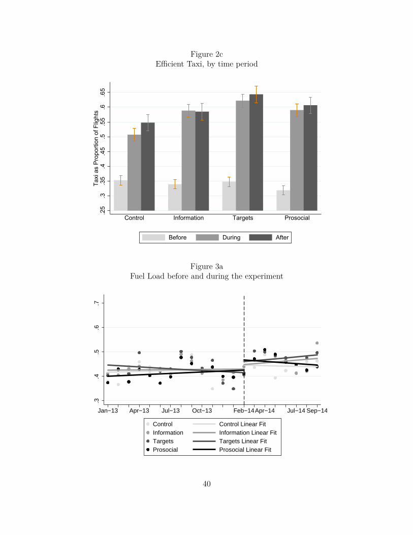
Figure 2cEfficient Taxi, by time period

.25

.3.3

5.4

.45

.5.5

5.6

.65

Taxi

as

Pro

porti

on o

f Flig

hts


Before During After

Figure 3aFuel Load before and during the experiment

.3.4

.5.6

.7

Jan−13 Apr−13 Jul−13 Oct−13 Feb−14 Apr−14 Jul−14 Sep−14

Control Control Linear FitInformation Information Linear FitTargets Targets Linear FitProsocial Prosocial Linear Fit

40

Figure 3bEfficient Flight before and during the experiment

.3.4

.5.6

.7



Figure 3cEfficient Taxi before and during the experiment

.3.4

.5.6

.7



41

Figure 4aTreatment effects for Fuel Load during the experiment

-.06

-.03

0.0

3.0

6.0

9.1

2.1

5.1

8Tr

eatm

ent E

ffect

as

Pro

porti

on o

f Flig

hts

Feb Mar Apr May Jun Jul Aug Sep

Information Targets Prosocial

Figure 4bTreatment effects for Efficient Flight during the experiment

-.06

-.03

0.0

3.0

6.0

9.1

2.1

5.1

8Tr

eatm

ent E

ffect

as

Pro

porti

on o

f Flig

hts



42

Figure 4cTreatment effects for Efficient Taxi during the experiment

-.06

-.03

0.0

3.0

6.0

9.1

2.1

5.1

8Tr

eatm

ent E

ffect

as

Pro

porti

on o

f Flig

hts



43

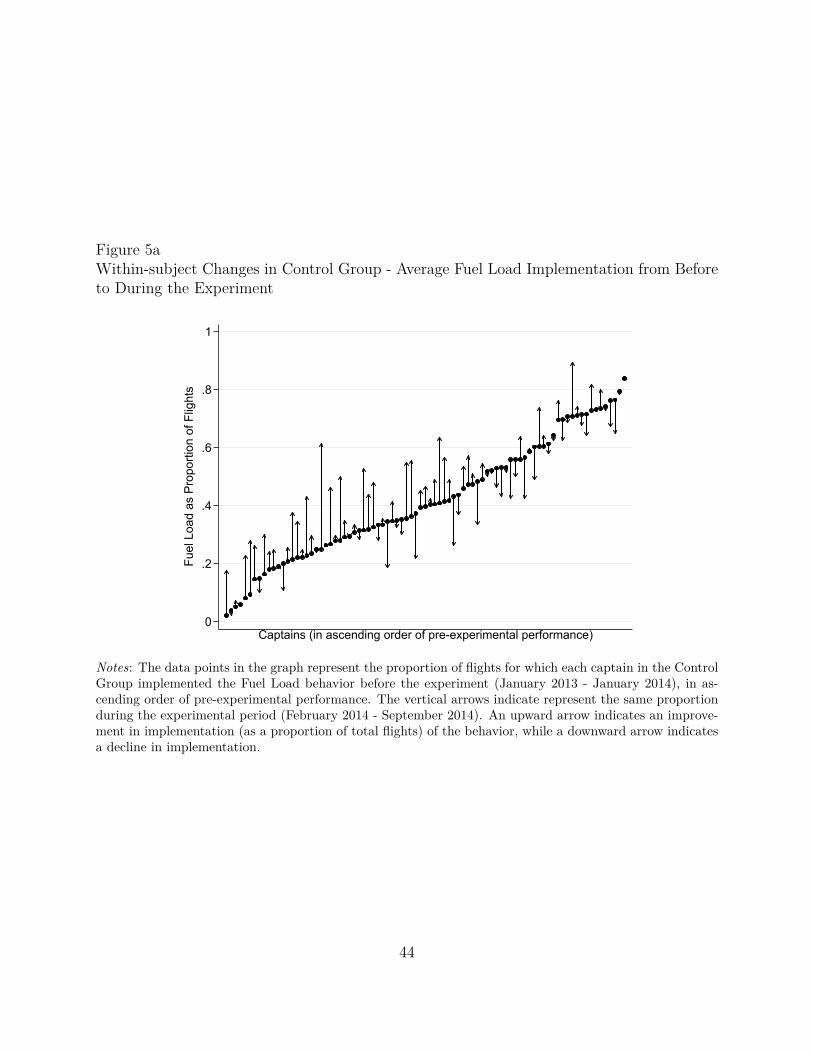
Figure 5aWithin-subject Changes in Control Group - Average Fuel Load Implementation from Beforeto During the Experiment

0

.2

.4

.6

.8

1

Fuel

Loa

d as

Pro

porti

on o

f Flig

hts

Captains (in ascending order of pre-experimental performance)

Notes: The data points in the graph represent the proportion of flights for which each captain in the ControlGroup implemented the Fuel Load behavior before the experiment (January 2013 - January 2014), in as-cending order of pre-experimental performance. The vertical arrows indicate represent the same proportionduring the experimental period (February 2014 - September 2014). An upward arrow indicates an improve-ment in implementation (as a proportion of total flights) of the behavior, while a downward arrow indicatesa decline in implementation.

44

Figure 5bWithin-subject Changes in Control Group - Average Efficient Flight Implementation fromBefore to During the Experiment

0

.2

.4

.6

.8

Effi

cien

t Flig

ht a

s P

ropo

rtion

of F

light

s


Notes: The data points in the graph represent the proportion of flights for which each captain in the ControlGroup implemented the Efficient Flight behavior before the experiment (January 2013 - January 2014), inascending order of pre-experimental performance. The vertical arrows represent the same proportion duringthe experimental period (February 2014 - September 2014). An upward arrow indicates an improvement inimplementation (as a proportion of total flights) of the behavior, while a downward arrow indicates a declinein implementation.

45

Figure 5cWithin-subject Changes in Control Group - Average Efficient Taxi Implementation fromBefore to During the Experiment

0

.2

.4

.6

.8

1

Taxi

as

Pro

porti

on o

f Flig

hts


Notes: The data points in the graph represent the proportion of flights for which each captain in the ControlGroup implemented the Efficient Taxi behavior before the experiment (January 2013 - January 2014), inascending order of pre-experimental performance. The vertical arrows represent the same proportion duringthe experimental period (February 2014 - September 2014). An upward arrow indicates an improvement inimplementation (as a proportion of total flights) of the behavior, while a downward arrow indicates a declinein implementation.

46

Figure 6aWithin-subject Changes in All Groups - Average Fuel Load Implementation from Before toDuring the Experiment (Net of Raw Hawthorne Effects)

0

.5

1

0

.5

1

Control Information

Targets Prosocial

Fuel

Loa

d as

Pro

porti

on o

f Flig

hts

47

Figure 6bWithin-subject Changes in All Groups - Average Efficient Flight Implementation from Beforeto During the Experiment (Net of Raw Hawthorne Effects)

-.5

0

.5

1

-.5

0

.5

1

Control Information

Targets Prosocial

Effi

cien

t Flig

ht a

s P

ropo

rtion

of F

light

s

48

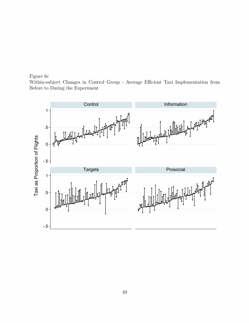
Figure 6cWithin-subject Changes in Control Group - Average Efficient Taxi Implementation fromBefore to During the Experiment

-.5

0

.5

1

-.5

0

.5

1

Control Information

Targets Prosocial

Taxi

as

Pro

porti

on o

f Flig

hts

49

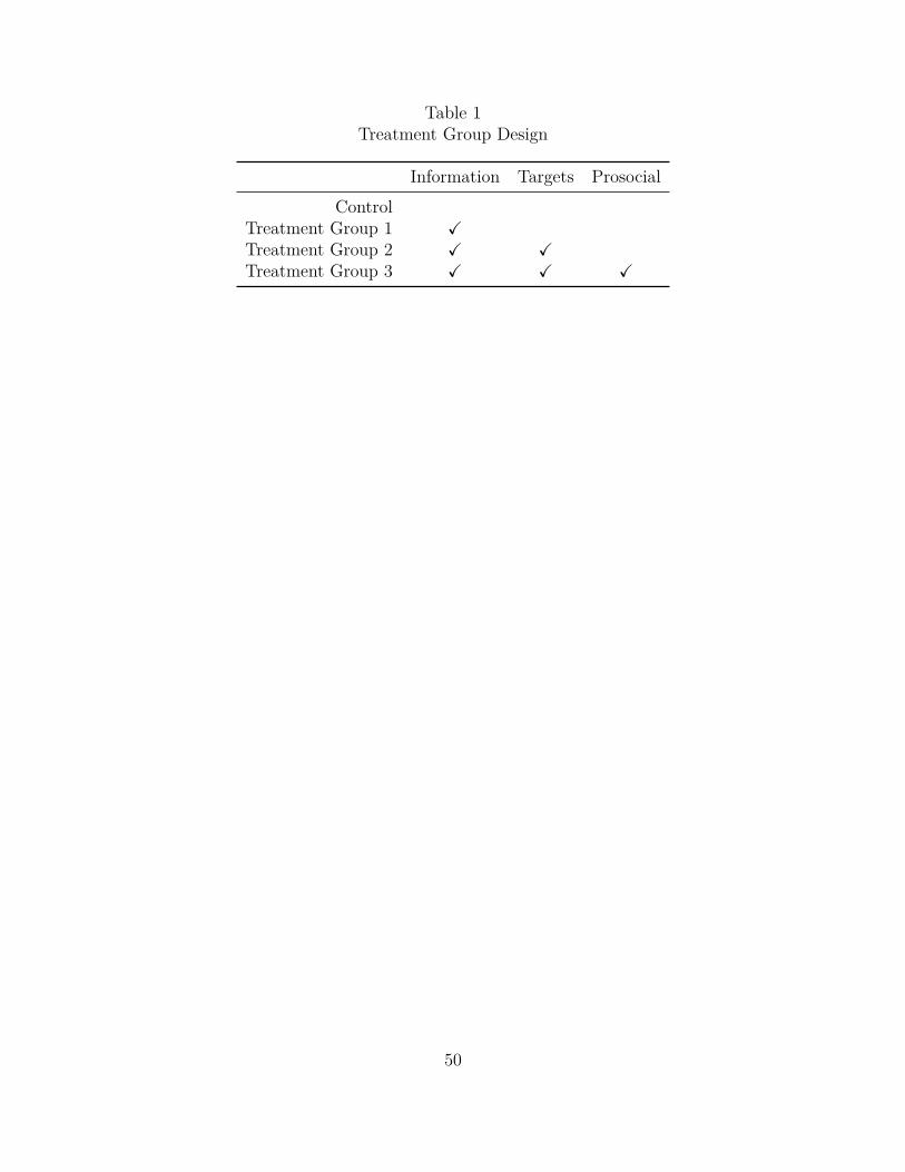
Table 1Treatment Group Design

Information Targets ProsocialControl

Treatment Group 1 XTreatment Group 2 X XTreatment Group 3 X X X

50

Table 2Average Attainment of Fuel Load, Efficient Flight, and Efficient Taxi in all Time Periods(Raw Data)

Control Treatment 1: Treatment 2: Treatment 3: All CaptainsInformation Targets Prosocial

Fuel Load

Before Experiment0.421 0.428 0.434 0.414 0.424(0.494) (0.495) (0.496) (0.493) (0.494)5258 obs 5429 obs 5070 obs 5140 obs 20,897 obs

During Experiment0.443 0.462 0.475 0.458 0.459(0.497) (0.499) (0.499) (0.498) (0.498)3321 obs 3330 obs 3016 obs 3258 obs 12,925 obs

After Experiment0.446 0.446 0.469 0.412 0.442(0.497) (0.497) (0.499) (0.492) (0.497)2140 obs 2120 obs 1867 obs 2063 obs 8190 obs

Efficient Flight


During Experiment0.476 0.503 0.528 0.510 0.504(0.500) (0.500) (0.499) (0.499) (0.500)3321 obs 3330 obs 3016 obs 3258 obs 12,925 obs


Efficient Taxi


During Experiment0.507 0.588 0.622 0.590 0.575(0.500) (0.492) (0.485) (0.492) (0.494)2117 obs 2109 obs 1864 obs 2014 obs 8104 obs


Notes: The table reports the proportion of flights for which captains in a given group performed each of thethree selected behaviors. Due to random memory errors, Efficient Taxi data is unavailable for 35.0% of pre-experimental flights and 37.2% of post-experimental flights. This missing data is in no way systematic andtherefore does not bias the results, though it moderately reduces the power of the Efficient Taxi estimates.Standard deviations are reported in parentheses, which is followed by the total number of observations(flights) from which the summary statistics are calculated.

51

Table 3Difference in Attainment from Before Experiment to During Experiment for all ExperimentalConditions

(1) (2) (3) (4) (5) (6)Fuel Load Eff Flight Eff Taxi Fuel Load Eff Flight Eff Taxi

Expt · Control 0.018 0.144*** 0.125*** 0.018* 0.144*** 0.125***(0.012) (0.012) (0.017) (0.011) (0.011) (0.013)

Expt · Information 0.025* 0.161*** 0.206*** 0.025** 0.161*** 0.206***(0.013) (0.012) (0.019) (0.011) (0.011) (0.013)

Expt · Targets 0.039*** 0.181*** 0.222*** 0.039*** 0.181*** 0.222***(0.015) (0.014) (0.022) (0.012) (0.011) (0.014)

Expt · Prosocial 0.043*** 0.191*** 0.214*** 0.043*** 0.191*** 0.214***(0.012) (0.013) (0.022) (0.011) (0.011) (0.013)

Observations 33,822 33,822 21,681 33,822 33,822 21,681N 335 335 335 335 335 335Controls Yes Yes Yes Yes Yes YesStandard Errors:Clustered Yes Yes YesNewey-West Yes Yes Yes

Notes: The table shows the results of two panel linear probability regressions with captain fixed effects forconventional robust standard errors and Newey-West standard errors with a lag of one period. The regressionscompare pre-experiment behavior (January 2013-January 2014) to behavior during the experiment ‘Expt’(February 2014-September 2014) for all experimental conditions, including the control group. We presentthe results of panel OLS specification—as opposed to those of panel logit or probit specifications—due toconstraints on the conditional logit/probit models, which cannot provide marginal effects due to lack ofestimation of fixed effects (i.e. intercepts), though results for post-estimation of the various models arenearly identical. The dependent variables in the regressions are dummies capturing whether the fuel-efficientbehavior was performed, and since predicted values are not constrained between 0 and 1, we do not reporta constant and instead focus on treatment effects. As such, the coefficients indicate the proportion of flightsfor which the behavior of interest was successfully performed. Robust errors are clustered at the captainlevel. Controls include weather on departure and arrival, number of engines on the aircraft, aircraft type,ports of departure and arrival, aircraft maintenance, captains’ contracted hours, and whether the captainhas completed training. ∗∗∗p < 0.01 ∗∗p < 0.05 ∗p < 0.10

52

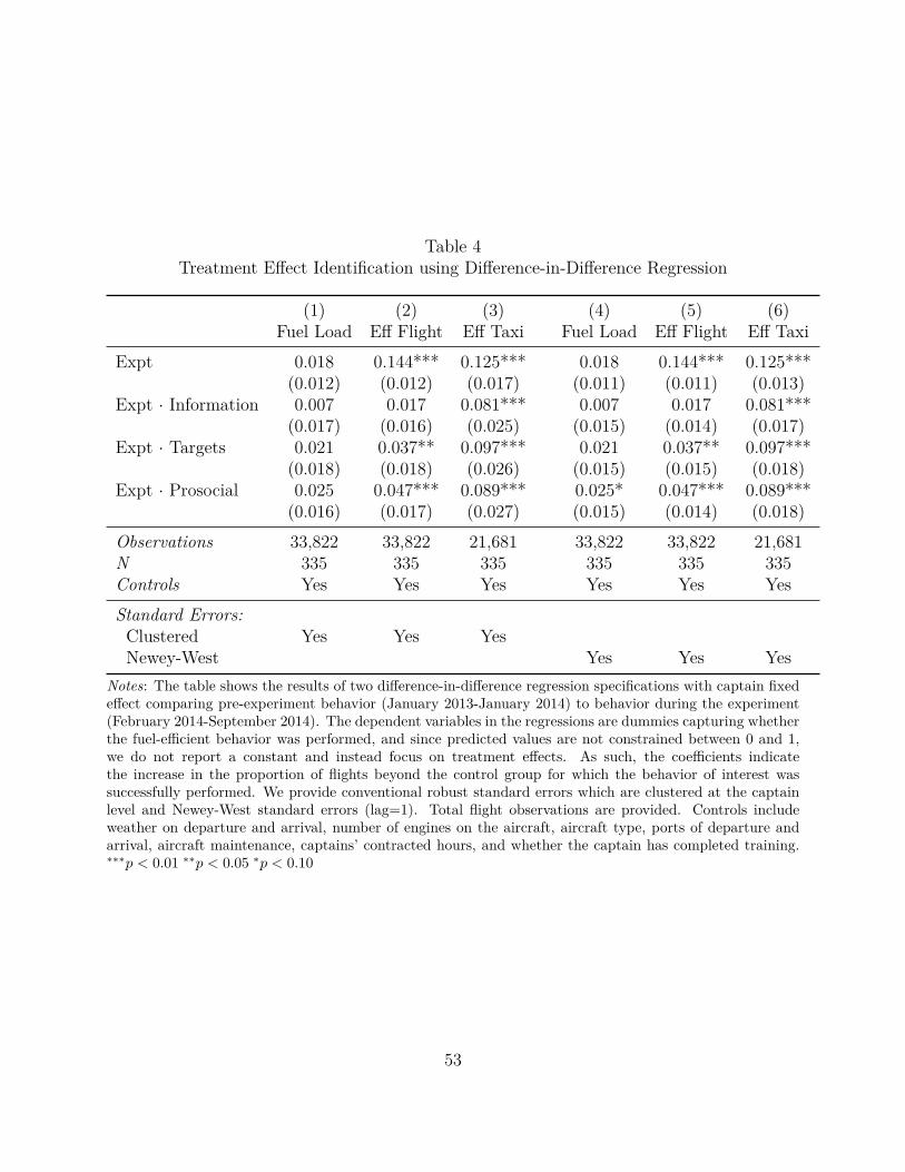
Table 4Treatment Effect Identification using Difference-in-Difference Regression


Expt 0.018 0.144*** 0.125*** 0.018 0.144*** 0.125***(0.012) (0.012) (0.017) (0.011) (0.011) (0.013)

Expt · Information 0.007 0.017 0.081*** 0.007 0.017 0.081***(0.017) (0.016) (0.025) (0.015) (0.014) (0.017)

Expt · Targets 0.021 0.037** 0.097*** 0.021 0.037** 0.097***(0.018) (0.018) (0.026) (0.015) (0.015) (0.018)

Expt · Prosocial 0.025 0.047*** 0.089*** 0.025* 0.047*** 0.089***(0.016) (0.017) (0.027) (0.015) (0.014) (0.018)


Notes: The table shows the results of two difference-in-difference regression specifications with captain fixedeffect comparing pre-experiment behavior (January 2013-January 2014) to behavior during the experiment(February 2014-September 2014). The dependent variables in the regressions are dummies capturing whetherthe fuel-efficient behavior was performed, and since predicted values are not constrained between 0 and 1,we do not report a constant and instead focus on treatment effects. As such, the coefficients indicatethe increase in the proportion of flights beyond the control group for which the behavior of interest wassuccessfully performed. We provide conventional robust standard errors which are clustered at the captainlevel and Newey-West standard errors (lag=1). Total flight observations are provided. Controls includeweather on departure and arrival, number of engines on the aircraft, aircraft type, ports of departure andarrival, aircraft maintenance, captains’ contracted hours, and whether the captain has completed training.∗∗∗p < 0.01 ∗∗p < 0.05 ∗p < 0.10

53

Table 5Persistence: Difference in Attainment from Before Experiment to After Experiment for allExperimental Conditions


Post · Control 0.049** 0.215*** 0.152*** 0.049** 0.215*** 0.152***(0.024) (0.021) (0.035) (0.021) (0.020) (0.029)

Post · Information 0.042* 0.195*** 0.192*** 0.042** 0.195*** 0.192***(0.022) (0.023) (0.040) (0.021) (0.019) (0.030)

Post · Targets 0.067*** 0.218*** 0.209*** 0.067*** 0.218*** 0.209***(0.023) (0.023) (0.037) (0.021) (0.019) (0.030)

Post · Prosocial 0.029 0.217*** 0.210*** 0.029 0.217*** 0.210***(0.025) (0.021) (0.037) (0.021) (0.019) (0.030)


Notes: The table shows the results of two panel linear probability regressions with captain fixed effectsfor conventional robust standard errors and Newey-West standard errors with a lag of one period. Theregressions compare pre-experiment behavior (January 2013-January 2014) to post-experiment behavior(“Post”: October 2014-March 2015) for all experimental conditions, including the control group. We presentthe results of panel OLS specification—as opposed to those of panel logit or probit specifications—due toconstraints on the conditional logit/probit models, which cannot provide marginal effects due to lack ofestimation of fixed effects (i.e. intercepts), though results for post-estimation of the various models arenearly identical. The dependent variables in the regressions are dummies capturing whether the fuel-efficientbehavior was performed, and since predicted values are not constrained between 0 and 1, we do not reporta constant and instead focus on treatment effects. As such, the coefficients indicate the proportion of flightsfor which the behavior of interest was successfully performed. Robust errors are clustered at the captainlevel. Controls include weather on departure and arrival, number of engines on the aircraft, aircraft type,ports of departure and arrival, aircraft maintenance, captains’ contracted hours, and whether the captainhas completed training. ∗∗∗p < 0.01 ∗∗p < 0.05 ∗p < 0.10

54

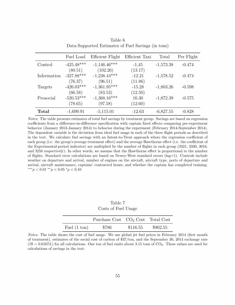
Table 6Data-Supported Estimates of Fuel Savings (in tons)

Fuel Load Efficient Flight Efficient Taxi Total Per FlightControl -425.48*** -1,146.46*** -1,45 -1,573.38 -0.474

(80.51) (102.26) (13.17)Information -327.88*** -1,238.44*** -12.21 -1,578.52 -0.474

(76.37) (96.51) (11.86)Targets -426.03*** -1,361.95*** -15.28 -1,803.26 -0.598

(66.58) (83.53) (12.50)Prosocial -520.53*** -1,368.16*** 16.30 -1,872.39 -0.575

(78.65) (97.58) (12.60)Total -1,699.91 -5,115.01 -12.63 -6,827.55 -0.828

Notes: The table presents estimates of total fuel savings by treatment group. Savings are based on regressioncoefficients from a difference-in-difference specification with captain fixed effects comparing pre-experimentbehavior (January 2013-January 2014) to behavior during the experiment (February 2014-September 2014).The dependent variable is the deviation from ideal fuel usage in each of the three flight periods as describedin the text. We calculate fuel savings with an Intent-to-Treat approach where the regression coefficient ofeach group (i.e. the group’s average treatment effect) and the average Hawthorne effect (i.e. the coefficient ofthe Experimental-period indicator) are multiplied by the number of flights in each group (3321, 3330, 3016,and 3258 respectively). In other words, we assume that the Hawthorne effect is proportional to the numberof flights. Standard error calculations are based on Newey-West standard errors (lag=1). Controls includeweather on departure and arrival, number of engines on the aircraft, aircraft type, ports of departure andarrival, aircraft maintenance, captains’ contracted hours, and whether the captain has completed training.∗∗∗p < 0.01 ∗∗p < 0.05 ∗p < 0.10

Table 7Costs of Fuel Usage

Purchase Cost CO2 Cost Total CostFuel (1 ton) $786 $116.55 $902.55

Notes: The table shows the cost of fuel usage. We use global jet fuel prices in February 2014 (first monthof treatment), estimates of the social cost of carbon of $37/ton, and the September 30, 2014 exchange rate(1$ = 0.6167£) for all calculations. One ton of fuel emits about 3.15 tons of CO2. These values are used forcalculations of savings in the text.

55

A Appendix I: Additional Tables

56

TableA1

VAA

Expe

riment-B

alan

ceTa

ble

Plan

Num

ber

Fligh

tsAbove

Above

Above

Trusted

Ram

pof

per

Average

Average

Average

Fue

lEfficient

Efficient

Group

sGen

der

Seniority

Age

Trainer

Pilot

Weekend

Fuel

Eng

ines

Mon

thPRF

NOE

FPM

Loa

dFligh

tTax

i

C,T1

1.00

00.27

20.73

50.68

70.70

00.30

90.83

10.74

90.88

90.53

90.64

51.00

00.92

00.61

30.39

1C,T2

0.56

00.67

80.43

00.83

80.65

00.27

30.86

00.75

50.84

40.44

30.87

80.87

80.89

90.68

30.39

0C,T3

0.56

00.96

20.91

80.55

10.65

00.87

90.71

90.89

80.63

70.16

70.75

90.75

90.96

00.51

20.60

3T1,

T2

0.56

00.51

90.62

70.84

30.40

60.95

70.96

90.99

10.72

60.87

80.75

90.87

80.81

70.92

50.99

5T1,

T3

0.56

00.29

90.65

30.84

60.40

60.21

90.89

20.85

10.51

60.44

30.87

80.75

90.96

00.88

00.77

9T2,

T3

1.00

00.71

50.37

00.69

51.00

00.18

70.85

80.85

80.78

50.53

90.87

80.64

50.85

90.81

10.77

5

Test

χ2

t-test

t-test

χ2

χ2

t-test

t-test

t-test

t-test

χ2

χ2

χ2

t-test

t-test

t-test

Not

es:The

numbersin

thetableare

p-values

forthecompa

risonof

means

across

treatm

entgrou

ps,whe

reC

deno

testheCon

trol

grou

p(n

=85

),T1de

notestheInform

ationgrou

p(n

=85

),T2

deno

testheTargets

grou

p(n

=81

),an

dT3de

notestheProsocial

grou

p(n

=84

).Respectively,treatm

entassign

mentwas

balanc

edon

captains’gend

er;seniority;

age;

traine

rstatus;Trusted

Pilot

status;prop

ortion

offlightsflow

non

weekend

s;flight

plan

rampfuel

(asaprox

yforaverag

edistan

ceflow

n);averag

enu

mber

ofen

gine

son

aircraft

flow

n;averag

enu

mber

offlightsflow

nper

mon

thin

thepre-experim

entalperiod;

indicators

forwhe

ther

thecaptains

ischaracterizedby

aboveaverag

eplan

rampfuel

(PRF),

number

ofen

gine

s(N

OE),

andflightsper

mon

th(F

PM);

andattainmentof

thethreeou

tcom

evariab

lesof

interest

(Fue

lLoa

d,EfficientFligh

t,an

dEfficientTax

i).

57

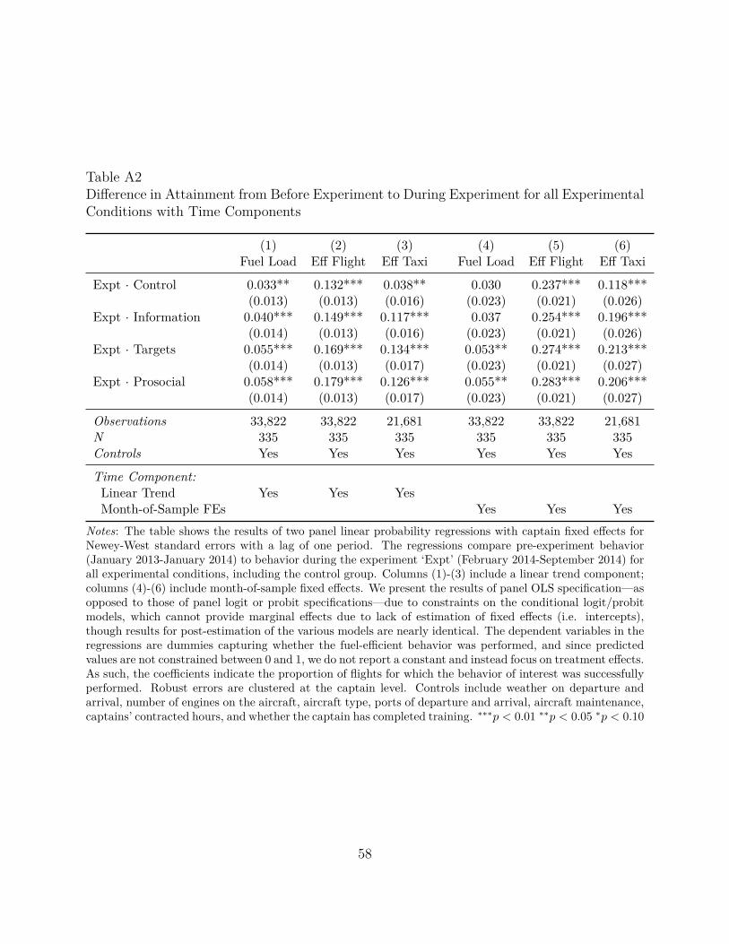
Table A2Difference in Attainment from Before Experiment to During Experiment for all ExperimentalConditions with Time Components


Expt · Control 0.033** 0.132*** 0.038** 0.030 0.237*** 0.118***(0.013) (0.013) (0.016) (0.023) (0.021) (0.026)

Expt · Information 0.040*** 0.149*** 0.117*** 0.037 0.254*** 0.196***(0.014) (0.013) (0.016) (0.023) (0.021) (0.026)

Expt · Targets 0.055*** 0.169*** 0.134*** 0.053** 0.274*** 0.213***(0.014) (0.013) (0.017) (0.023) (0.021) (0.027)

Expt · Prosocial 0.058*** 0.179*** 0.126*** 0.055** 0.283*** 0.206***(0.014) (0.013) (0.017) (0.023) (0.021) (0.027)

Observations 33,822 33,822 21,681 33,822 33,822 21,681N 335 335 335 335 335 335Controls Yes Yes Yes Yes Yes Yes

Time Component:Linear Trend Yes Yes YesMonth-of-Sample FEs Yes Yes Yes

Notes: The table shows the results of two panel linear probability regressions with captain fixed effects forNewey-West standard errors with a lag of one period. The regressions compare pre-experiment behavior(January 2013-January 2014) to behavior during the experiment ‘Expt’ (February 2014-September 2014) forall experimental conditions, including the control group. Columns (1)-(3) include a linear trend component;columns (4)-(6) include month-of-sample fixed effects. We present the results of panel OLS specification—asopposed to those of panel logit or probit specifications—due to constraints on the conditional logit/probitmodels, which cannot provide marginal effects due to lack of estimation of fixed effects (i.e. intercepts),though results for post-estimation of the various models are nearly identical. The dependent variables in theregressions are dummies capturing whether the fuel-efficient behavior was performed, and since predictedvalues are not constrained between 0 and 1, we do not report a constant and instead focus on treatment effects.As such, the coefficients indicate the proportion of flights for which the behavior of interest was successfullyperformed. Robust errors are clustered at the captain level. Controls include weather on departure andarrival, number of engines on the aircraft, aircraft type, ports of departure and arrival, aircraft maintenance,captains’ contracted hours, and whether the captain has completed training. ∗∗∗p < 0.01 ∗∗p < 0.05 ∗p < 0.10

58

Table A3Treatment Effect Identification using Difference-in-Difference Regression with QuadrupletControls


Expt 0.022 0.146*** 0.140*** 0.022** 0.146*** 0.140***(0.015) (0.013) (0.016) (0.010) (0.009) (0.011)

Expt · Information 0.017 0.023 0.065*** 0.017 0.023** 0.065***(0.020) (0.016) (0.022) (0.012) (0.011) (0.014)

Expt · Targets 0.022 0.041** 0.092*** 0.022* 0.041*** 0.092***(0.020) (0.016) (0.022) (0.012) (0.012) (0.015)

Expt · Prosocial 0.011 0.042*** 0.078*** 0.011 0.042*** 0.078***(0.019) (0.016) (0.023) (0.012) (0.011) (0.014)


Notes: The table shows the results of two difference-in-difference regression specifications with quadrupletfixed effects comparing pre-experiment behavior (January 2013-January 2014) to behavior during the exper-iment (February 2014-September 2014). The dependent variables in the regressions are dummies capturingwhether the fuel-efficient behavior was performed, and since predicted values are not constrained between 0and 1, we do not report a constant and instead focus on treatment effects. As such, the coefficients indicatethe increase in the proportion of flights beyond the control group for which the behavior of interest wassuccessfully performed. We provide conventional robust standard errors which are clustered at the captainlevel and Newey-West standard errors (lag=1). Total flight observations are provided. Controls includeweather on departure and arrival, number of engines on the aircraft, aircraft type, ports of departure andarrival, aircraft maintenance, captains’ contracted hours, and whether the captain has completed training.∗∗∗p < 0.01 ∗∗p < 0.05 ∗p < 0.10

59

Table A4Persistence: Treatment Effect Identification using Difference-in-Difference Regression com-paring Before Experiment to After Experiment for all Experimental Conditions


Post 0.049** 0.215*** 0.152*** 0.049** 0.215*** 0.152***(0.024) (0.021) (0.035) (0.021) (0.020) (0.029)

Post · Information -0.007 -0.021 0.040 -0.007 -0.021 0.040*(0.020) (0.021) (0.030) (0.017) (0.016) (0.021)

Post · Targets 0.018 0.003 0.057** 0.018 0.003 0.057***(0.020) (0.022) (0.026) (0.018) (0.017) (0.022)

Post · Prosocial -0.020 0.002 0.058** -0.020 0.002 0.058***(0.021) (0.020) (0.025) (0.017) (0.016) (0.021)


Notes: The table shows the results of two difference-in-difference regression specifications with captainfixed effect comparing pre-experiment behavior (January 2013-January 2014) to post-experiment behavior(“Post”: October 2014-March 2015). The dependent variables in the regressions are dummies capturingwhether the fuel-efficient behavior was performed, and since predicted values are not constrained between 0and 1, we do not report a constant and instead focus on treatment effects. As such, the coefficients indicatethe increase in the proportion of flights beyond the control group for which the behavior of interest wassuccessfully performed. We provide conventional robust standard errors which are clustered at the captainlevel and Newey-West standard errors (lag=1). Total flight observations are provided. Controls includeweather on departure and arrival, number of engines on the aircraft, aircraft type, ports of departure andarrival, aircraft maintenance, captains’ contracted hours, and whether the captain has completed training.∗∗∗p < 0.01 ∗∗p < 0.05 ∗p < 0.10

60

Table A5Data-Supported Estimates of Average Fuel Savings per Flight (in kilograms)

Fuel Load Efficient Flight Efficient TaxiControl -128.12*** -345.21*** -0.43

(24.24) (30.79) (3.97)Information -98.46*** -371.90*** -3.67

(22.93) (28.98) (3.56)Targets -141.26*** -451.57*** -5.07

(22.07) (27.69) (4.14)Prosocial -159.77*** -419.94*** 5.00

(24.14) (29.95) (3.87)Notes: The table presents estimates of average fuel savings by treatment group. Savings are based on re-gression coefficients from a difference-in-difference specification with captain fixed effects comparing pre-experiment behavior (January 2013-January 2014) to behavior during the experiment (February 2014-September 2014). The dependent variable is the deviation from ideal fuel usage in each of the three flightperiods as described in the text. We calculate fuel savings with an Intent-to-Treat approach where wesum the regression coefficient of each group (i.e. the group’s average treatment effect) and the averageHawthorne effect (i.e. the coefficient of the Experimental-period indicator). In other words, we assume thatthe Hawthorne effect is constant across grous. Standard error calculations are based on Newey-West stan-dard errors (lag=1). Controls include weather on departure and arrival, number of engines on the aircraft,aircraft type, ports of departure and arrival, aircraft maintenance, captains’ contracted hours, and whetherthe captain has completed training. ∗∗∗p < 0.01 ∗∗p < 0.05 ∗p < 0.10

Table A6Test of a Unit Root of Pre-Experiment Behaviors

Fuel Load Eff Flight Eff TaxiZ(t) -3.765*** -2.562* -6.431***

(0.003) (0.010) (0.000)Observations (weeks) 51 51 51

Notes: The table shows the Dickey-Fuller (DF) test for a unit root for the 51 weeks before the experimentstarted, collapsing all the groups into one for each behavior. The null of the DF test is a unit root, and therejection of the null is that the data follows a random walk. Z(t) is the DF test statistic. ∗∗∗p < 0.01 ∗∗p <0.05 ∗p < 0.10

61

Table A7Difference-in-Difference Regression of Flight Time

Flight TimePost 1.788***

(0.522)Post · Information 0.011

(0.687)Post · Targets 0.114

(0.733)Post · Prosocial -1.586*

(0.849)N 335 subjectsObservations 33,822Controls Yes

Notes: The dependent variable in this regression is flight time in minutes. Captain fixed effects are includedand Newey-West standard errors (lag = 1) are reported below estimates in parentheses. Total flight obser-vations are provided. Controls include weather on departure and arrival, number of engines on the aircraft,aircraft type, ports of departure and arrival, aircraft maintenance, captains’ contracted hours, and whetherthe captain has completed training. ∗∗∗p < 0.01 ∗∗p < 0.05 ∗p < 0.10

62

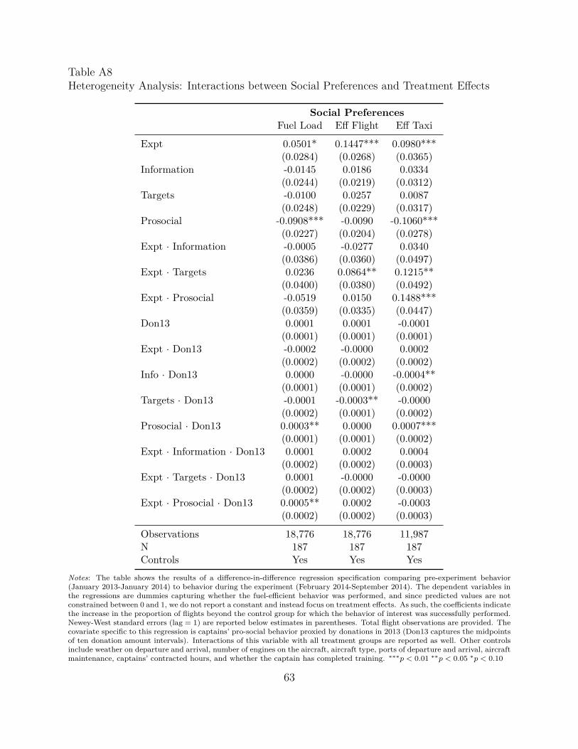
Table A8Heterogeneity Analysis: Interactions between Social Preferences and Treatment Effects

Social PreferencesFuel Load Eff Flight Eff Taxi

Expt 0.0501* 0.1447*** 0.0980***(0.0284) (0.0268) (0.0365)

Information -0.0145 0.0186 0.0334(0.0244) (0.0219) (0.0312)

Targets -0.0100 0.0257 0.0087(0.0248) (0.0229) (0.0317)

Prosocial -0.0908*** -0.0090 -0.1060***(0.0227) (0.0204) (0.0278)

Expt · Information -0.0005 -0.0277 0.0340(0.0386) (0.0360) (0.0497)

Expt · Targets 0.0236 0.0864** 0.1215**(0.0400) (0.0380) (0.0492)

Expt · Prosocial -0.0519 0.0150 0.1488***(0.0359) (0.0335) (0.0447)

Don13 0.0001 0.0001 -0.0001(0.0001) (0.0001) (0.0001)

Expt · Don13 -0.0002 -0.0000 0.0002(0.0002) (0.0002) (0.0002)

Info · Don13 0.0000 -0.0000 -0.0004**(0.0001) (0.0001) (0.0002)

Targets · Don13 -0.0001 -0.0003** -0.0000(0.0002) (0.0001) (0.0002)

Prosocial · Don13 0.0003** 0.0000 0.0007***(0.0001) (0.0001) (0.0002)

Expt · Information · Don13 0.0001 0.0002 0.0004(0.0002) (0.0002) (0.0003)

Expt · Targets · Don13 0.0001 -0.0000 -0.0000(0.0002) (0.0002) (0.0003)

Expt · Prosocial · Don13 0.0005** 0.0002 -0.0003(0.0002) (0.0002) (0.0003)

Observations 18,776 18,776 11,987N 187 187 187Controls Yes Yes Yes

Notes: The table shows the results of a difference-in-difference regression specification comparing pre-experiment behavior(January 2013-January 2014) to behavior during the experiment (February 2014-September 2014). The dependent variables inthe regressions are dummies capturing whether the fuel-efficient behavior was performed, and since predicted values are notconstrained between 0 and 1, we do not report a constant and instead focus on treatment effects. As such, the coefficients indicatethe increase in the proportion of flights beyond the control group for which the behavior of interest was successfully performed.Newey-West standard errors (lag = 1) are reported below estimates in parentheses. Total flight observations are provided. Thecovariate specific to this regression is captains’ pro-social behavior proxied by donations in 2013 (Don13 captures the midpointsof ten donation amount intervals). Interactions of this variable with all treatment groups are reported as well. Other controlsinclude weather on departure and arrival, number of engines on the aircraft, aircraft type, ports of departure and arrival, aircraftmaintenance, captains’ contracted hours, and whether the captain has completed training. ∗∗∗p < 0.01 ∗∗p < 0.05 ∗p < 0.10

63

Table A9Job Satisfaction and Treatment Group

Job SatisfactionInformation 0.212

(0.224)Targets 0.0242

(0.249)Prosocial 0.365

(0.224)Constant 5.58***

(0.174)N 202

Notes: The dependent variable in this regression is a 7-point scale of job satisfaction, where self-reportedjob satisfaction increases in the scale. Robust standard errors are reported below estimates in parentheses.∗∗∗p < 0.01 ∗∗p < 0.05 ∗p < 0.10

Table A10Job Satisfaction and Job Performance

Groups Control and Information Targets and ProsocialJob Satisfaction Job Satisfaction

Fuel Load Targets Met 0.042 - 0.065 -(0.052) (0.060)

Eff Flight Targets Met -0.071 - -0.017 -(0.056) (0.054)Eff Taxi Targets Met 0.037 - 0.120** -(0.038) (0.054)

Overall Targets Met - 0.000 - 0.058*(0.025) (0.025)

Constant 5.714*** 5.687*** 5.341*** 5.326***(0.263) (0.258) (0.358) (0.326)

N N=103 subjects N=99 subjectsObs 103 99Controls None None

Notes: The dependent variable in these regressions is a 7-point scale of job satisfaction, where self-reportedjob satisfaction increases in the scale. Robust standard errors are reported below estimates in parentheses.The independent variables indicate the number of targets met per behavior and overall over the course ofthe study. ∗∗∗p < 0.01 ∗∗p < 0.05 ∗p < 0.10

64

B Appendix II: Theoretical Model

B.1 Model Setup

We consider a static choice-problem that determines a captain’s chosen effort on the job in acertain period. In our model, we assume that captains, who have vast flying experience, areat an equilibrium fuel usage with respect to their wealth, experience, effort, and concernsfor safety, the environment, and company profitability.50

A captain faces the following additively separable utility function:

U(w, s, e, f, g) = u(w, e, g) + a · v(d(e) · g, g0, G−i) + y(s, e, f)− c(e)− s(e) (1)

where u(·) is utility from monetary wealth, v(·) is utility from giving to charity (pro-socialbehavior), y(·) is utility from job performance, c(·) is disutility from exerting effort, ands(·) describes disutility from social pressure. Effort is chosen for all three flight tasks, j,i.e. Fuel Load, Efficient Flight, and Efficient Tax. Captains observe their effort perfectly.They also receive a noisy signal of fuel usage fit + εit = fit. fit describes the estimatedfuel usage by captain i for flight t which depends on the chosen effort for the fuel-efficientactivities. fit is actual fuel use, observed ex post by the airline, which also includes a randomcomponent.51 Furthermore, each captain has an ideal fuel usage fI , which is based on herown experience and environmental and firm profit preferences. By revealed preference theequilibrium pre-study fuel usage fI = f .

Experimental treatments in this study alter three model parameters. First, receivinginformation on fuel use, i = 1(information), removes the noisiness of the fuel signal, i.e.fit + (1− i)εit = fit. Second, provision of a target, r = 1(target), changes the captain’s idealfuel usage, fI , because the employer exogenously imposes a target level. Then, fI = fT ifr = 1 where fT reflects the signaled optimal usage from the point of view of the airline.Third, in the pro-social behavior treatment a donation, g, is made by the airline in the nameof the captain. This donation is conditional on meeting the target which has a probability

50In a survey, captains in the study expressed a concern over fuel usage and fuel cost, both for environ-mental reasons and company profitability. To become an airline captain requires many years of training andexperience within an airline; if a captain loses her job with one airline and seeks employment in another, sheloses her prior seniority and must work for many years to reinstate it. Thus, for the sake of their own jobsecurity, captains care about minimizing fuel costs.

51Due to the vast experience of captains, we assume E(εit) = 0, i.e. captains predict fuel usage correctly,on average.

65

of d(e) in this treatment.52 In all other treatments, reaching particular fuel use levels doesnot lead to donations, i.e. d(e) = 0. Parameters and elements of the utility function areexplained in more detail below.

(Dis)utility from social pressure. In the spirit of DellaVigna et al. (2012, “DLM” here-after) and Bénabou and Tirole (2006), we assume that captains are either affected by socialpressure due to their actions being observed or exhibit some sort of social signaling in whichthey want to appear to be good employees. In this framework, captains are aware of an op-timal, social effort level, esocial. Because exerting effort is costly to the captain and becauseher actions are imperfectly observed with probability πobserved < 1, generally e < esocial.53

In this study, captains in both the control group and treatment group are made aware thattheir actions are monitored and data on their effort are used for an internal and academicstudy. Consequently, we expect the probability of detection of deviations from the socialeffort level to increase for all participants in the study relative to the pre-study period, i.e.πobservedstudy > πobservedpre . We parameterize social pressure as follows:

s(e) = [πobserved · (esocial − e) + (1− πobserved) · 0] · 1(e < esocial)

Social pressure decreases utility if the chosen effort level is below the socially optimaleffort level of the captain. This disutility is increasing in the distance from the optimaleffort level and in the probability of these actions being observed by the airline. The secondterm captures the fact that unobserved deviations do not lead to disutility. For agents thatexert more effort than esocial, s(e) simply drops out of their utility function. Consequently,captains can directly impact the level of disutility by exerting more (costly) effort.

Note that s(e) enters the utility of every captain below the social effort level, regardless oftreatment assignment. If social pressure is important, even control captains should respondto this increased cost of low effort.54 Because s(e) is orthogonal to treatment, we omit it in

52Captains can directly influence the probability with their effort. That is, captains can be certain thatthey do not meet a target if they put in little effort, and they can be certain that they have achieved thetarget if they put in sufficient effort.

53It is plausible to argue that effort is perfectly observed in the aviation industry with modern technology.However, captains might not expect these data to be analyzed on a regular basis.

54Alternatively, we could interpret esocial as a level of effort induced by the researcher, leading toexperimenter-demand effects. Put differently, pilots in the study could think they are expected to increaseeffort and not doing so imposes utility costs on them.

66

the following discussion and in the derivation of comparative statics.55

Utility from wealth. Similar to DLM, for wealth w, charitable giving from the airline gfor meeting the target (if applicable), and other charitable giving g0, u is defined as follows:

u(w, e, g) = u(w − g0(d(e) · g) + a · d(e) · g)

where a =

0 if a < 0

a if 0 ≤ a ≤ 1

1 if a > 1

Private consumption is an individual’s wealth minus the amount given to charity fromthat person’s wealth (i.e. not from this study). However, to ensure that u is continuouslydifferentiable, we need to account for the effect of charitable donations resulting from ourtreatments on utility from private consumption. To capture this effect, we multiply theindividual’s expected donation, d(e)·g, by a function of a—a parameter capturing preferencesfor giving—which we call a. As in DLM, the parameter a is non-negative in the case of pureor impure altruism and negative in the case of spite56, and a is simply a truncated at 0 and1.

The reasons for creating such boundaries on the term capturing preferences for giving aretwofold. First, an individual with spiteful preferences (a < 0) does not get less utility fromprivate consumption when she donates to charity than when she does not donate to charity;therefore, a is censored from below at 0. Second, an individual with pure or impure altruisticpreferences will get additional utility from her private consumption by giving to charitythrough our treatment because it corresponds to an outward shift in the budget constraintin the dimension of giving to the chosen charity. However, a is censored from above at 1because an individual will experience weakly more utility from increases in w than fromgiving to the chosen charity (i.e. ∂u

∂w≥ ∂u

∂g). This relation holds since increases in w shift the

budget constraint outward in all dimensions—including the charitable giving dimension—so55Social pressure is additively separable from other utility elements in a linear model. Consequently, it

does not affect the sign of comparative statics derived below and, if interactions are present, only attenuatestreatment effect estimates.

56As defined in Andreoni (1989, 1990), pure and impure altruism capture two possible motivations forgiving. The first stems from a preference solely for provision of the public good, so that an individual’sdonations are entirely crowded out by donations from other sources. Impure altruism, on the other hand,refers to the phenomenon whereby individuals receive direct utility from the act of giving itself, i.e. through“warm glow”. Spite, as defined in DLM, exists when an individual gets disutility from donating to the charity.

67

these must be weakly preferred to shifts in only one dimension. This stipulation is importantto assume differentiability in u in a standard expected utility framework, as in DLM.

Please note that the amount an individual gives to other charities will be related to theamount that she gives to charity in the context of this study. Captains will smooth theirconsumption for giving. If a captain normally gives $100 to charity each year and this yearshe gives $10 through the context of the study, we would expect her total giving to bebetween $100 and $110, or g0 + g ∈ [100, 110]. The realization of the sum depends on thevalue of a and whether a stems from pure altruism, impure altruism, or spite. We shouldexpect that an individual who has a negative a value does not donate to charity outside ofthe context of this study since donating to charity decreases that individual’s utility.

Utility from charitable giving. The v term is also adapted from DLM and follows thesame properties for each type of individual (pure or impure altruistic and spiteful). Themain difference between the v term in this study and that in DLM is that in this study,not everyone has the opportunity to donate to charity (i.e. d(e) > 0 for only one treatmentgroup). We also assume that v is separable in its parameters, as follows:

v(d(e) · g, g0, G−i) = v1(d(e) · g,G−i) + v2(θg0, G−i)

where θ is the cost of giving through channels other than the study and G−i is total giving byother individuals. In this specification, v1 represents utility from giving in the study contextand v2 represents utility from giving from one’s personal wealth. Note that v1(0, G−i) = 0since if d(e) = 0, then a captain is not able to donate to the charity through the contextof the study, so v1 should not affect the utility function (similar to the spite case). Basedon the arguments made above with respect to consumption smoothing, v|d=0 ≤ v|d=p, 0 =v1|d=0 ≤ v1|d=p, v2|d=0 ≥ v2|d=p. That is, a captain’s utility from giving is at least as highfor those captains for whom d(e) = p as it is for those captains for whom d(e) = 0, whichfollows from our assumption that giving in the study context can only decrease giving fromone’s own wealth or not affect it at all. Finally, since ∂p

∂e> 0, we have ∂v

∂e≥ 0.

In the case of pure altruism, an individual should get the same utility from giving tocharity from her personal wealth as from giving to charity through the context of the study,since the benefit to the charity is identical. In this sense, v can be thought to representthe charity’s production function. In the case of impure altruism, an individual should alsoget the same utility from donating to charity through her personal wealth as she does fromdonating through the context of the study because the amount donated on her behalf is the

68

same. Lastly, in the case of spite, g0 = 0 since giving to charity decreases utility and so thoseindividuals will not give to charity independently of the study. Note, v(0) = 0 because if aperson does not give to charity in person then her utility from giving to charity in person is0.

Utility from job performance. Since captains care about fuel efficiency, and since imposingexogenous targets on performance affects a captain’s perception of how well she is doing herjob, we include a parameter y capturing job performance.57 We assume y is separable insafety (s) and fuel (f) because changes in fuel as a result of the study do not affect safetylevels, as argued in our assumption above. A captain whose performance exceeds her targetwill achieve higher utility under this parameter than a captain who does not achieve hertarget. Similarly, a captain will experience less (more) utility the further below (above)the target is her performance. We therefore incorporate job performance into the model asfollows:

y(s, e, f) = y1(s) + y2(e, f) = y1(s) + y2(−f | − fI)

where

y2(−f | − fI) = y2m(−f) + y2n(−f | − fI)

and

y2n(−f | − fI) = r · µ(y2m(−f)− y2m(−fI))

Here, y2 is defined as in Köszegi and Rabin (2006, “KR” hereafter). We denote the com-ponents of y2 “m” and “n” to mirror the notation in KR. As in KR, m represents the“consumption utility” and n represents the “gain-loss utility.” These terms are separableacross dimensions. Finally, µ is the “universal gain-loss function” and has the associateproperties outlined in KR. To be clear, we use the targets in our second treatment group asan exogenous reference point that airline captains perceive as a reference point.

Note that pilots get utility from using less fuel ∂y2∂f≤ 0 and, conditional on receiving

a reference point, get utility (disutility) from performing above (below) the target, which57Evidence indicates that influencing job performance positively influences job satisfaction (or utility),

whether through increased self-esteem or perceived managerial support for autonomous decision-making(Christen et al., 2006; Pugno and Depedri, 2009).

69

increases with distance from the target according to µ. We assume µ is linear and µ(x) = ηx

if x > 0 and µ = ηλx if x ≤ 0 for η > 0, λ > 1, in accordance with theories of loss aversion.Moreover, following naturally from our definition of µ, we assume y(x) = x. If a captaindoes not receive a reference point, her utility does not comprise gain-loss utility, so for theseindividuals y2 = y2m. That is, if r = 0, captains do not receive information regarding idealperformance with respect to fuel efficiency, so their job performance parameter dependssolely on fuel consumption.58

Additionally, based on industry standards and emphasis on safety—as well as the designof the treatments—we assume that captains’ job performance utility from flying safely isconstant across treatments, therefore:

∂y

∂s= S ≥ 0

(Dis)utility from effort. Finally, c represents the cost of effort. Importantly, the individual

cost functions for each fuel-efficient task are allowed to differ to convey that various taskshave different costs associated with them. The cost structure is a function of the difficultyof the task itself (e.g., it may be easier to turn off one engine after landing than to havean efficient flight for several hours) and resistance due to previous habit formation (e.g.,captains who for many years have not properly performed the Zero Weight Fuel calculationmay find it difficult or bothersome to begin doing so). Additionally, the costs for each taskare separable since the tasks are done independently. Therefore,

c(e) =∑j

cj(ej)

For a captain to decrease her fuel use, she must also increase her effort, i.e. ∂f∂e< 0. Note

that c(e) is subtracted in the utility equation, so ∂U∂c< 0, ∂c

∂e> 0. Based on interviews with

captains, the cost of effort increases at an increasing rate. Defining the cost of effort as aquadratic function of effort implies that the cost of effort increases with the amount of effortexerted (i.e. ∂2c

∂e2 > 0).58To be clear, given that our reference point is exogenously imposed, one cannot clearly assess whether

the individual captain is better off in the targets group than in another group.

70

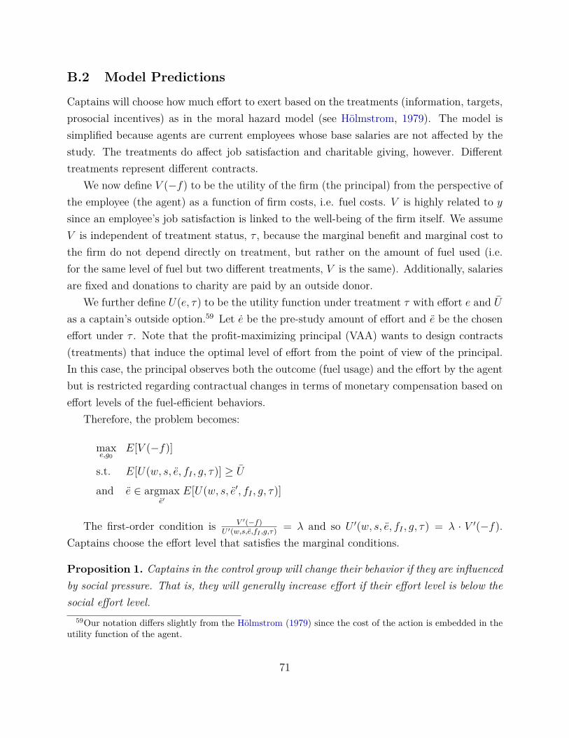
B.2 Model Predictions

Captains will choose how much effort to exert based on the treatments (information, targets,prosocial incentives) as in the moral hazard model (see Hölmstrom, 1979). The model issimplified because agents are current employees whose base salaries are not affected by thestudy. The treatments do affect job satisfaction and charitable giving, however. Differenttreatments represent different contracts.

We now define V (−f) to be the utility of the firm (the principal) from the perspective ofthe employee (the agent) as a function of firm costs, i.e. fuel costs. V is highly related to ysince an employee’s job satisfaction is linked to the well-being of the firm itself. We assumeV is independent of treatment status, τ , because the marginal benefit and marginal cost tothe firm do not depend directly on treatment, but rather on the amount of fuel used (i.e.for the same level of fuel but two different treatments, V is the same). Additionally, salariesare fixed and donations to charity are paid by an outside donor.

We further define U(e, τ) to be the utility function under treatment τ with effort e and Uas a captain’s outside option.59 Let e be the pre-study amount of effort and e be the choseneffort under τ . Note that the profit-maximizing principal (VAA) wants to design contracts(treatments) that induce the optimal level of effort from the point of view of the principal.In this case, the principal observes both the outcome (fuel usage) and the effort by the agentbut is restricted regarding contractual changes in terms of monetary compensation based oneffort levels of the fuel-efficient behaviors.

Therefore, the problem becomes:

maxe,g0

E[V (−f)]

s.t. E[U(w, s, e, fI , g, τ)] ≥ U

and e ∈ argmaxe′

E[U(w, s, e′, fI , g, τ)]

The first-order condition is V ′(−f)U ′(w,s,e,fI ,g,τ) = λ and so U ′(w, s, e, fI , g, τ) = λ · V ′(−f).

Captains choose the effort level that satisfies the marginal conditions.

Proposition 1. Captains in the control group will change their behavior if they are influencedby social pressure. That is, they will generally increase effort if their effort level is below thesocial effort level.

59Our notation differs slightly from the Hölmstrom (1979) since the cost of the action is embedded in theutility function of the agent.

71

Proof: We argued above that scrutiny due to the intervention is likely to (weakly) increaseeither the probability of detection of a sub-optimal effort level (πobserved) or the perceivedlevel of socially optimal level of effort (esocial) or both. Both effects increase the social costcomponent of the utility function for captains in all treatment cells, including the controlgroup. Put differently, for a given level of effort e < esocial, the intervention increases themarginal social cost of exerting low effort ∂U

∂s|e. Consequently, captains respond to these

new marginal conditions and increase their effort if they are below the (perceived) sociallyoptimal level.60

Proposition 2. Information will cause captains to increase or decrease their effort andthereby increase or decrease fuel usage respectively or choose the outside option, dependingon the realization of the difference between estimated (fit) and actual (fit) fuel usage (i.e.the value of the parameter εit).

Proof: Let the pre-study period be t = 0 and the study period be t = 1.Assume in period t = 0, εi0 < 0, then fi0 > fi0, so that when captains receive information

in t = 1, they learn that y2m(−f) > E[y2m(−f)]. In other words, they were more fuel-efficientin t = 0 than they expected to be. Therefore, if they provide the same level of effort in periodt = 1, they will experience a level of utility greater than their pre-study equilibrium. Theypay the same cost of effort but receive more utility from job satisfaction. They will thenweakly decrease their chosen level of effort. How much depends on the functional form ofthe y and c functions and their pre-study effort level. Captains in the information or targetstreatments—where wealth and the charities’ production functions are independent of effort—will not decrease their effort if y is steeper than c around their chosen values. This scenariois possible since there is a random shock of εi0 to their location of −f and we are agnosticabout the functional form of y. Without the shock, they would not be in equilibrium if ywere steeper with respect to effort than c at the chosen level of effort because they couldincrease effort and pay a slightly higher cost but get much more utility from job satisfaction.They will not choose their outside option since if

E[U(w, s, e, fI , g, τ = “pre-study, no treatment”)] ≥ U ,

60Because of orthogonality to treatment, this simply increases baseline effort. Furthermore, because utilityis additively separable, qualitative findings from the subsequent comparative statics analysis are unchanged.If there are interactions between social pressure and the treatments, these interactions just attenuate pointestimates because all treatments are designed to increase effort against a now greater baseline.

72

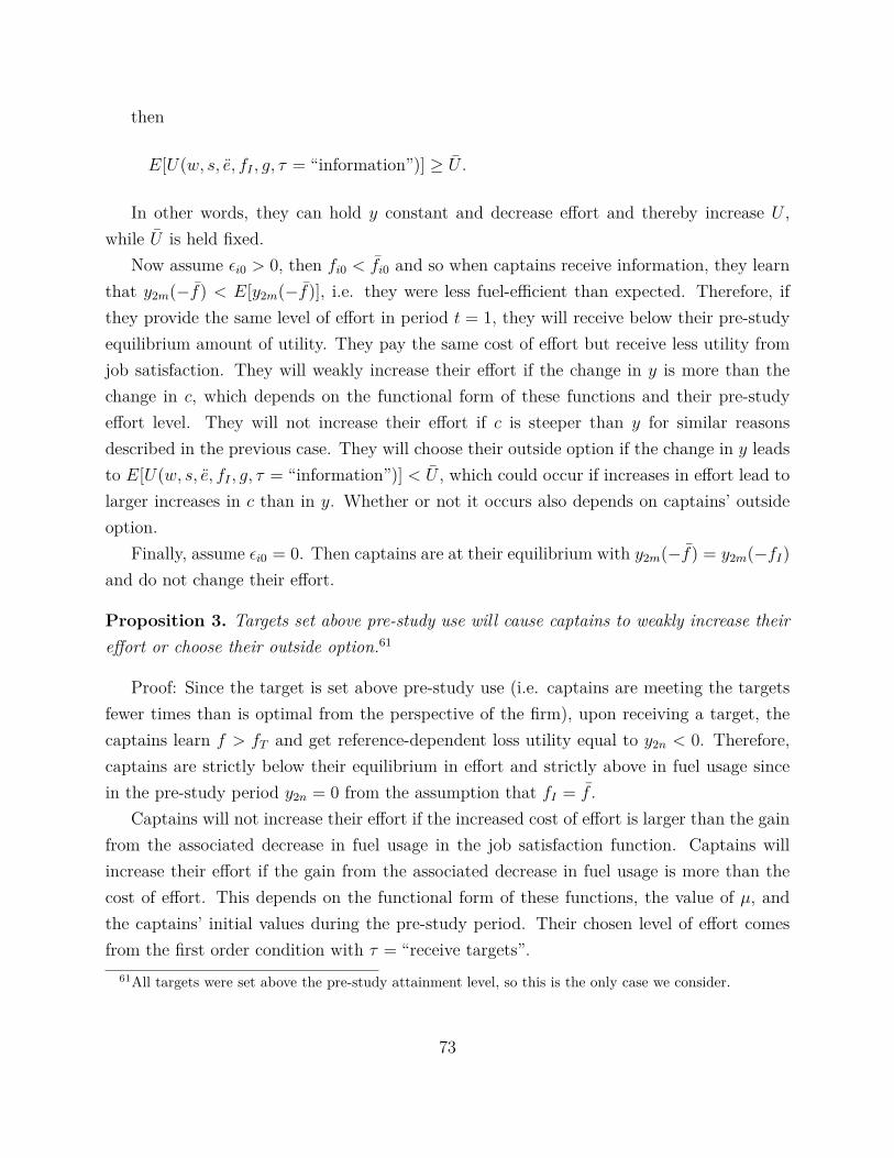
then

E[U(w, s, e, fI , g, τ = “information”)] ≥ U .

In other words, they can hold y constant and decrease effort and thereby increase U ,while U is held fixed.

Now assume εi0 > 0, then fi0 < fi0 and so when captains receive information, they learnthat y2m(−f) < E[y2m(−f)], i.e. they were less fuel-efficient than expected. Therefore, ifthey provide the same level of effort in period t = 1, they will receive below their pre-studyequilibrium amount of utility. They pay the same cost of effort but receive less utility fromjob satisfaction. They will weakly increase their effort if the change in y is more than thechange in c, which depends on the functional form of these functions and their pre-studyeffort level. They will not increase their effort if c is steeper than y for similar reasonsdescribed in the previous case. They will choose their outside option if the change in y leadsto E[U(w, s, e, fI , g, τ = “information”)] < U , which could occur if increases in effort lead tolarger increases in c than in y. Whether or not it occurs also depends on captains’ outsideoption.

Finally, assume εi0 = 0. Then captains are at their equilibrium with y2m(−f) = y2m(−fI)and do not change their effort.

Proposition 3. Targets set above pre-study use will cause captains to weakly increase theireffort or choose their outside option.61

Proof: Since the target is set above pre-study use (i.e. captains are meeting the targetsfewer times than is optimal from the perspective of the firm), upon receiving a target, thecaptains learn f > fT and get reference-dependent loss utility equal to y2n < 0. Therefore,captains are strictly below their equilibrium in effort and strictly above in fuel usage sincein the pre-study period y2n = 0 from the assumption that fI = f .

Captains will not increase their effort if the increased cost of effort is larger than the gainfrom the associated decrease in fuel usage in the job satisfaction function. Captains willincrease their effort if the gain from the associated decrease in fuel usage is more than thecost of effort. This depends on the functional form of these functions, the value of µ, andthe captains’ initial values during the pre-study period. Their chosen level of effort comesfrom the first order condition with τ = “receive targets”.

61All targets were set above the pre-study attainment level, so this is the only case we consider.

73

Since captains experience a negative utility shock from receiving a target, they will choosethe outside option if E[U(w, s, e, fI , g, τ = “receive targets”)] ≤ U .

Proposition 4. Donations made to charity for meeting targets will weakly increase effort ifcaptains’ altruism is strictly positive and the donations do not affect their effort otherwise.

Proof: Let Vc(d(e), g) be the production function of the charity. Note that in the case ofpure altruism Vc = v1, as defined in the previous section. ∀d(e) · g ≥ 0, we have Vc > 0 andVc = 0 if and only if d(e) · g = 0. Then, captains solve the following optimization problem:

maxe,g0

E[V (−f) + a · Vc]

s.t. E[U(w, s, e, fI , g, τ)] ≥ U

and e ∈ argmaxe′

E[w, s, e′, fI , g, τ)]

with first-order condition V ′(−f)+a·V ′cU ′(w,s,e,f,g,τ) = λ. If a captain has zero altruism, i.e. a = 0, then

this equation reduces to the original and effort does not increase above the effect describedin Proposition 1. If a > 0, then the numerator of the first-order condition is weakly largerthan the control case. It is strictly larger if d > 0. Captains with strictly positive altruismmay choose an effort level corresponding to d = 0 if the additional cost of increased effortrequired for meeting the target is more than the gain in utility from donating to charity.The probability of this occurring is decreasing in the level of altruism.

Since λ is a constant, increases in the sum of the production functions of the firm andcharity cause increases in effort, e < e.

Proposition 5. Captains in the targets and prosocial conditions will choose to increase theireffort the most in tasks for which the targets are easiest to meet.

Proof: Since the firm sets the targets and donations exogenously62, the utility for meetinga target is constant across tasks. The donation to charity is the same across tasks as ex-ogenously determined, and since the targets are also exogenously determined, the captainsbelieve that the firm values them all equally by revealed preference. If the firm did notvalue them equally, then it would not offer the same reward. However, the cost function isnot constant across tasks for reasons described earlier, which implies that the captains will

62Note that the “firm” here refers to both VAA and the academic researchers, who jointly made mostdecisions with respect to experimental design.

74

choose to increase their effort on tasks for which targets are easiest to meet.63 Within ourairline context, the least effortful behavior to attain is Efficient Taxi, followed by Fuel Load,then Efficient Flight. The determination of this ordering is based on discussions with manyairline captains and trusted pilots groups.

63Our theory and interventions are rooted in Hölmstrom’s 1979 “Informativeness Principle”, which statesthat any accessible information about an agent’s effort should be used in the design and enforcement ofoptimal contracts. Our interventions are not aimed at the efficient allocation of effort across these tasks—asproposed in Hölmstrom and Milgrom (1991) and Baker (1992)—since we assume our three behaviors arenot substitutable (since they occur during different phases of flight). We acknowledge the possibility thatadditional fuel-efficient behaviors exist that we do not measure that may be fully or partially neglected dueto our treatments.

75

C Appendix III: Examples of Treatment Groups

Figure A1Treatment Group 1: Information

We will continue to keep you updated on your monthly performance for the next X months, John.

Please see reverse side for further details of the three behaviours.

Questions? We are here to help! Please email us at [email protected].

Fuel and carbon efficiency report for Capt. John Smith

Below is your monthly fuel and carbon efficiency report for Month 2014

1. ZERO FUEL WEIGHT Proportion of flights for which the ZFW calculation was completed and fuel load adjusted as necessary

RESULT: XX% of flights

2. EFFICIENT FLIGHT Proportion of flights for which actual fuel use is less than planned fuel use (e.g. optimised speed, altitude etc)


3. REDUCED ENGINE TAXY IN Proportion of flights for which at least one engine was shut off during taxy in


All data gathered during this study will remain anonymous and confidential. Safety remains the absolute and overriding priority. This study will be carried out within Virgin’s existing and highly robust safety standards, using our existing fuel procedures and policies. Captains retain full authority, as they always have done in VAA, to make decisions based on their professional judgment and experience.

76

Figure A2Treatment Group 2: Targets

WHAT WAS YOUR OVERALL OUTCOME?

You achieved X of your 3 targets last month.

WELL DONE! We will continue to keep you updated on your monthly performance for the next X months, John.

Please continue to fly efficiently next month to achieve your targets.






TARGET: XX% of flights


You ACHIEVED/MISSED your target.










77

Figure A3Treatment Group 3: Prosocial

WHAT WAS YOUR OVERALL OUTCOME?

Due to your fuel and carbon efficient decision making last month, you achieved X of your 3 targets and secured £XX of a possible £30

for your chosen charity, Charity Name.

WELL DONE! For the next X months, you still have the ability to donate £X to Charity Name. Please continue to fly efficiently next month to achieve your targets so your

charity does not lose out.








You ACHIEVED/MISSED your target and

earned/missed out on £10 in donations to Charity

Name. .






Name.






Name. .


78

Figure A4All Treatment Groups: Reverse Side of Report

THE THREE BEHAVIOURS WE ARE MEASURING

Behaviour 1: Zero Fuel Weight Adjustment (ZFW) - Pre Flight

This measure compares Actual Ramp against Plan Ramp adjusted for changes in ZFW. It captures whether a double iteration adjustment has been implemented for ZFW in line with Plan Burn Adjustment and any further amendments to flight plan fuel that have been entered into ACARS. This behaviour has a tolerance of 200kg, which ensures that rounding in the fuel request / loading procedure will not adversely affect the result. Behaviour 2: Efficient Flight (EF) - During Flight

This measure examines the actual fuel burn per minute compared against the expected fuel burn per minute from OFF to ON (expected fuel burn is Plan Trip adjusted for ZFW). It highlights pilot technique (e.g. optimum settings are realised, optimum levels are sought, speed is optimised, etc.). Behaviour 3: Reduced Engine Taxy In (RETI) - Post Flight

This measure observes if an engine has been shut down during taxy in. RETI is considered to have taken place if one engine burns less than 70% of the average of other engines during taxy in. If taxy in is shorter than the cool down period required, the flight is omitted, as RETI was not possible.

We hope the above information is beneficial to you. If you require more information about any of the behaviours, please email us at [email protected].

79

D Appendix IV: Survey Materials

D.1 Prosocial Incentives

80

D.2 Job Satisfaction

81